Metallgesellschaft: A Prudent Hedger Ruined or a Wildcatter on NYMEX?

The Journal of Futures Markets, Vol. 17, No. 5, 543–578 (1997)Q 1997 by John Wiley & Sons, Inc. CCC 0270-7314/97/050543-36

Metallgesellschaft: APrudent Hedger

Ruined, or aWildcatter on NYMEX?

STEPHEN CRAIG PIRRONG

INTRODUCTIONThe travails of the firm Metallgesellschaft (MG) have received much at-tention in both academic circles and the financial press. The battle lineson the issue are clearly drawn. On one side, critics of MG [includingMello and Parsons, (1995)] claim that the firm’s energy market tradingwas rashly speculative, and as a result of adverse movements in oil prices,the firm suffered real mark-to-market losses of as much as one billiondollars. On the other side, defenders of the firm—notably Culp and Miller(1994)—claim that the firm employed a prudent and potentially very lu-crative strategy of hedging long-term energy delivery obligations withshort-term futures and swaps. In this view, MG’s bankers mistook a mereliquidity problem resulting from margin calls on futures positions for afull-blown insolvency crisis, unwisely unwound the firm’s hedge position,and prematurely terminated some of its long-term delivery contracts.

Which view is correct ultimately depends upon the dynamics of en-ergy prices, and how these dynamics affect optimal hedge ratios. MGimplemented a barrel-for-barrel hedge. That is, it bought one barrel ofshort-term energy futures or swaps for each barrel of oil it was committedto deliver, regardless of whether it was obligated to deliver in 6 monthsor 10 years. There are strong reasons to believe a priori that this hedgingstrategy forced the firm to bear more risk than necessary. However, Culpand Miller defend the one-for-one hedge, claiming that MG employed aninnovative synthetic storage (or carrying charge hedging) strategy that

■ Stephen C. Pirrong is an Assistant Professor of Finance at Washington University.

544 Pirrong

increased firm value while protecting MG against spot price increasesover the 10-year life of the program. They recognize that this strategyforced the firm to bear basis risk, but claim that this basis risk was smallrelative to the risk inherent in the firm’s fixed price contracts.

A definitive resolution of this debate cannot be achieved through apriori argument; the data must be the ultimate arbiter. This article un-dertakes a thorough analysis of the dynamics of crude oil futures pricesto determine the riskiness of the barrel-for-barrel strategy relative to al-ternative strategies available to the firm. This analysis of variance mini-mizing hedge ratios is more thorough and employs more sophisticatedeconometric techniques than previous studies by Mello and Parsons(1995) and Edwards and Canter (1995). It thus allows a more completecritique of the prudence of the barrel-for-barrel strategy.

The empirical results are starkly revealing. Given the behavior ofcrude oil prices, the variance-minimizing hedge ratio during 1993 was farless than 1. Indeed, for delivery obligations with maturities as short as 15months, the variance-minimizing hedge ratio was around 0.5, implyingthat MG’s barrel-for-barrel hedge actually increased the firm’s exposureto oil price risk. Even under very conservative assumptions the data implythat MG’s exposure to energy price risk was greater with a barrel-for-barrel futures and swap hedge than it would have been if the firm hadnot hedged its long-term delivery commitments at all! Consideration ofoptions embedded in the firm’s cash market contracts does not alter thefundamental result. Moreover, the prospect of earning gains every timeit rolled over its futures positions did not justify taking this additionalrisk. Thus, it is impossible to view the firm’s strategy as a prudent exercisein risk management.

The empirical results imply that the combined futures–long-termcontract position exposed the company to severe losses in the event of asteepening of the term structure of energy prices. This indeed occurredin 1993. Simulation estimates of the profitability of the barrel-for-barrelstrategy during this period imply that the firm lost approximately $800million on a mark-to-market basis. These estimates, which correspondclosely to accounting estimates of MG’s losses, contradict the claim thatthe firm’s losses were a mirage caused by misleading accounting standardsthat failed to reflect mark-to-market gains on its deferred deliverycontracts.

II. MG’s ENERGY MARKET ACTIVITIES

The details of MG’s energy market activities have been the subject ofmuch coverage, so a short overview will suffice here. In 1991, an MG

Metallgesellschaft 545

subsidiary—MG Refining and Marketing—entered the business of sup-plying American heating oil and gasoline retailers. To do so, it offeredthese retailers unprecedented 5- and 10-year fixed-price contracts. Thesecontracts were of two types. The firm-fixed contracts specified deliveryschedules. The firm-flexible contracts allowed buyers to choose the de-livery schedule with certain restrictions. Under the firm-flexible con-tracts, buyers were allowed to defer or accelerate purchases, but wererequired to buy all quantities deferred by the end of the contract. Thus,these contracts permitted buyers to choose the timing of deliveries, butnot their quantity. These contracts also allowed the buyers to terminateat will. At termination of the firm-fixed contracts, the buyers received apayment of one-half of the difference between the prevailing spot priceof West Texas Intermediate light crude oil and the fixed price in the con-tract, multiplied by the quantity remaining under the contract. Under thefirm-flexible contracts, the buyers received the full difference betweenthe 2-month futures price and the contract price.

By September 1993, MG had entered contracts obligating it to de-liver 102 million barrels of refined products under firm-fixed contracts.The tenor of 94% of these contracts was 10 years; the remainder had a5-year tenor. MG was obligated to deliver 47.5 million barrels of productsunder 10-year firm-flexible contracts, and 10.5 million under 5-year firm-flexible deals. Approximately one-third of these obligations were enteredinto during September 1993. In addition, MG entered into an arrange-ment to purchase refined products from Castle Energy Corp., a smallU.S. refiner. MG agreed to supply the refinery with most of the 100,000barrels per day (b/d) of crude oil it required, and agreed to purchase therefinery’s daily output of 40,000 b/d of gasoline and 35,000 b/d of heatingoil and other distillates.

To protect itself against increases in energy prices, MG purchasedcrude oil and gasoline futures contracts, and entered into OTC energyswaps. Rather than matching the expiration dates of the futures contractswith the dates of its delivery obligations to Castle and its customers, MGbought primarily near-month (i.e., next to expire) crude oil and gasolinecontracts. In the terminology of the futures trade, this is referred to as astacked hedge, because all hedging positions are stacked on a single con-tract month rather than spread over several contract months. MG’s OTCswaps were also of relatively short maturity. The expirations of these con-tracts were predominately less than or equal to three months. MG pur-chased one 1000 barrel futures contract or its swap equivalent for each1000 barrels of the firm’s short position regardless of the expiration dateof the short position. That is, the firm hedged barrel-for-barrel, and thus

546 Pirrong

by mid-to-late 1993 had bought 160,000,000 barrels of futures and swapsto cover its 160,000,000 barrel cash market position.

III. THE DETERMINATION OF HEDGE RATIOSTO CREATE A SYNTHETIC FORWARDPOSITION

A. Introduction

The riskiness of a barrel-for-barrel hedging strategy depends cruciallyupon the dynamics of energy prices. To see why, consider a firm thatdesires to minimize the variance of the payoff on a deferred forward de-livery obligation (the short position) in crude oil. This focus on varianceminimization is not intended to imply that only variance-minimizinghedges were appropriate for MG. Instead, variance minimization servesas a benchmark against which to measure actual trading strategies; bycomparing actual hedge ratios to variance minimizing ratios, it is possibleto quantify (a) the speculative component of a trading strategy, and (b)the risk of the actual trading strategy.

The fixed price in the forward obligation to be hedged is f. MG wasshort a bundle of many forward positions, but because the analysis isidentical for each forward contract in the bundle, for simplicity the anal-ysis focuses upon hedging a single element of the bundle; repeating thefollowing analysis for each element produces the appropriate hedge ratiofor MG’s entire swap position.

Assume that the firm is constrained to employ a single hedging in-strument—the next-to-expire crude oil futures contract (the nearby con-tract).1 The deferred obligation expires at time T. The firm can adjust thenumber of nearby contracts it buys at M equally spaced times betweentime t0 (the present) and T. That is, the firm can hedge dynamically. Eachinterval is Dt 4 (T 1 t0)/M in length. Because the nearby crude contractsexpire monthly, each interval is less than or equal to 1 month in duration.As M grows arbitrarily large, the firm effectively employs a continuouslyadjusted dynamic hedging strategy. Through this strategy, the firm at-tempts to replicate the payoffs to a forward position, thereby creating asynthetic forward contract.

1In general, it is not optimal to rely upon only a single hedging instrument. If there are multiplesources of risk in oil prices (e.g., the term structure shifts up and down and twists) then a firm canenjoy better hedging effectiveness if it uses several hedging instruments. The approaches describedbelow can be used to determine multiple-instrument hedge ratios. The very fact that MG employedonly the nearby contract strongly suggests that they were not interested in hedging alone, but werealso speculating on movements in the term structure.


The change in the price of a unit of the deferred over a time intervalending at t equals DFt,T [ Ft,T 1 Ft1Dt,T, where Ft,T is the forward priceat t for delivery at T. Because the payoff to the deferred delivery obligationoccurs at time T, and because MG is short, the change in the presentvalue of the deferred obligation is vt,T [ 1e1r(T1t) The change in2DF .t,T

the price of the nearby contract over the same time interval equals DSt

[ St 1 StDt. Because futures contracts are marked to market, the hedgerrealizes this gain or loss when it occurs. At t 1 Dt the firm buys bt,T unitsof the nearby contract to hedge each unit of its deferred obligation overthe interval, [t 1 Dt,t]. By T, the firm’s realized profit/loss equals

Mr(T t i t)1 1 D0P 4 e [b DS 1 Dv .o t i t,T t i t t i t,T F0 0 0 t ,TT ` D ` D ` D ] 1 0

i 14

The firm’s objective at t0 is to minimize (PT 1 PT)2.3E Et t0 0

Determination of the variance-minimizing hedge strategy for each trequires the solution of an extremely complex dynamic programmingproblem that allows the hedge ratio at t to depend upon expected hedgeratios for t8 . t [Chan (1992); Duffle and Jackson (1991), and Lien andLuo (1994)]. If mean price changes are nonzero, even in relatively simplecases involving time-varying spot and forward price dynamics, solution ofthis dynamic programming problem is not practical even for M on theorder of 2 or 3. It is therefore necessary to approximate the optimal dy-namic variance minimizing hedging solution by a sequence of myopichedge ratios which minimize the variance of the one-period hedge gain/loss; that is, the bt,T that minimizes Et1Dt [bt,T DSt 1 Dvt,T 1 Et1Dt Pt]

2

for t 4 t0 ` i Dt, i 4 1, . . . , M, where Pt 4 bt,T DSt 1 Dvt,T. This isthe approach taken in other studies of hedging with time-varying param-eters, such as Kroner and Sultan (1991).

2For simplicity, the analysis assumes that interest rates are nonstochastic, and the term structure ofinterest rates is flat. This expression holds because the value of the forward contract equals e1r(T1t)

( f 1 Ft,T). If interest rates are stochastic, futures prices and forward prices may differ due to theeffect of marking to market on the timing of cash flows. Cox, Ingersoll, and Ross (1981) demonstratethat this effect is important only to the extent that changes in interest rates and futures prices arecorrelated. Because the correlations between crude oil returns and percentage changes in interestrates are extremely small, this consideration is ignored hereafter. Specifically, over the July, 1987–June, 1994 period, the correlation between the percentage change in the 3-month T-bill rate and thepercentage change in the spot oil price is 0.01; the correlations between the percentage change inthe percentage changes in the 6- and 12-month T-bill rates and the percentage changes in futuresprices with 6 and 12 months to expiration, respectively, are less than 0.005.3For simplicity, it is assumed that the firm’s hedging horizon corresponds to the maturity of thedelivery obligation. This is not necessary. It is possible to choose a hedging horizon that is less thanthis maturity. Under the martingale assumption employed below, however, the firm optimally employsa myopic hedge ratio that is independent of the hedging horizon.

548 Pirrong

In the present case, the use of a series of single-period variance-minimizing hedges to approximate dynamically optimized hedges likelyinvolves little cost in terms of accuracy. The Appendix shows that myopichedge ratios are equal to those produced as the solution to the dynamicprogramming problem if St and Ft,T are martingales. [See also Duffie andJackson, (1991)], Section V.B shows that one cannot reject the hypothesisthat past price changes do not explain current price changes for eithernearby and deferred futures, which justifies the use of myopic hedge ra-tios even in a dynamic hedging problem.

It is well known that the optimal bt,T for one-period-ahead hedgingis given by

r(T t)1 1cov(DS , Dv ) e cov (DF , DS )t,T t,Tt tb 4 1 4 . (1)t,T var(DS ) var(DS )t t

This can be rewritten as:

r(DF )t,Tr(T t)1 1b 4 e corr (DF , DS ), (2)t,T t,T tr(DS )t

where r(DFt,T) is the standard deviation in interval in the change in theprice of the deferred obligation i r(DSt) is the standard deviation of thechange in the nearby price, and corr(DFt,T, DSt) is the correlation betweenthe change in the nearby price and the change in the deferred price.4

These correlations and variances may change over time for a varietyof reasons. First, it is plausible a priori that oil prices are stationary [Dixitand Pindyck (1994)]. Stationarity causes the volatility of the deferred torise as time passes. Second, the theory of storage implies that the vari-ances and correlations should depend upon the spread between spot anddeferred prices (net of interest and storage costs). When supplies areshort, the market is in backwardation. An increase in the severity of back-wardation causes an increase in both spot and deferred volatilities, a de-crease in the ratio of deferred volatility to spot volatility, and a decline inthe correlation between spot and deferred prices [Ng and Pirrong (1994)].

4The discount factor multiplying the correlation/standard deviation term reflects the fact that cashflows on the forward contracts are not received until the delivery date. Adjusting for this deferral ofcash flows by reducing the hedge ratio by the discount factor is called tailing the hedge. This consid-eration is relevant only to the extent that (a) the hedge position is large enough to permit a matchbetween the size of the tailed hedge and an integer number of futures contracts, and (b) the time todelivery is long enough to make the effect of discounting appreciable. Both cases are certainly relevantin the MG case. Therefore, MG could have and should have tailed its hedges to reflect cash-flowtiming mismatches between forwards and futures.


Because backwardation is a random variable, this implies that hedge ra-tios should change randomly as well. Third, shocks to the oil market (dueto OPEC policy changes, for example) can cause changes in the relevantvariances and correlations, and, thus, in hedge ratios. Given these threefactors, variance-minimizing hedging requires a methodology for quan-tifying how the relevant correlation and variances change. There are avariety of means to address this problem. This next section describes aGARCH-based methodology because it can take each of these factors intoaccount.5

B. Backwardation-Adjusted GARCH

Backwardation-adjusted GARCH (BAG) is a two-stage technique thatadjusts variances and covariances to reflect the three factors noted in theprior section. See Ng-Pirrong (1994, 1996) for a detailed presentation ofthis technique. In the first stage, to model the mean return of the nearbyand the deferred, one regresses the change in the nearby (deferred) priceagainst lagged changes in nearby and deferred prices and the lagged levelof backwardation. This latter variable is defined as

z 4 {ln[F 1 w(T 1 t ` 1)] 1 ln S }/(T 1 t ` 1) 1 r.t11 t11,T t11

In words, it is the percentage difference between the actual futures priceand the full-carry price calculated from the spot price, the cost of storage,w, and the interest rate.6 The residual from the spot equation is et, andthe residual from the futures equation is gt. In the second stage, one usesthe residuals from the mean equations to estimate jointly a modifiedGARCH model of the conditional variances and covariances of the nearbyand deferred return. In addition to the traditional GARCH terms, thismodel includes the squared lagged backwardation as an explanatory vari-able. This allows variances and covariances to depend upon the degreeof backwardation in the market. This model is estimated with the use ofquasimaximum likelihood. Formally, the equations for the conditionalvariance of the deferred return, hF,t, and the conditional variance of thenearby return, hS,t are

5Earlier drafts of this article included hedge-ratio estimates based on alternative methodologies,including backwardation adjusted regression, and factor models. These methods are cruder in crucialaspects than the GARCH, so these results are not reported here. The relevant results are availableon request.6One cannot observe the actual value of w. It is estimated in the following way. Arbitrage precludeszt . 0; that is, prices cannot be above full carry. Therefore, the value of the smallest w is found, suchthat, zt , 0 for all maturities and all days. This value is used as the estimate of w.

550 Pirrong

2 2h 4 x ` d h ` d e ` d z , (3)S,t S,t11 t11 t1S 1 2 3

2 2h 4 x ` f h ` f g ` r z . (4)F,t F,t11 t11 t11F 1 2 3

The inclusion of the terms allows the degree of backwardation to2zt 11

affect volatility. The conditional spot-forward covariance is

2r 4 q h h ` hz (5)!S,F,t S,t F,t t11

A GARCH model that does not include a backwardation term can alsobe employed to determine hedge ratios:

2h 4 x ` d h ` d e , (38)S,t S,t11 t11S 1 2

2h 4 x ` f h ` f g , (48)F,t F,t11 t11F 1 2

r 4 x ` l r ` l e g . (58)S,F,t S,F S,F,t11 t11 t111 2

This model does not allow the variance-covariance matrix of spot andfutures returns to depend upon backwardation, but does allow the co-variance between spot and futures residual returns at t to depend uponthe lagged covariance, and the product of the lagged residuals.

In each model, hedge ratios are given by

F rt,T S,F,tr(T t)1 1b 4 e .t,T S hS,tt

C. Summary and Implications

The BAG model allows the estimation of time-varying variance-minimiz-ing hedge ratios that reflect how fundamental supply-and-demand con-ditions affect the dynamics of energy prices. On a priori grounds thereare strong reasons to believe that hedge ratios should be far less than 1,especially for distant-deferred obligations.

Culp and Miller (CM) (1995a) object to the variance-minimizingframework for a variety of reasons. First, they claim that estimates ofvariance-minimizing hedge ratios are imperfect because data are “subjectto considerable error.” This is true, but estimates of hedge ratios that areconditional upon data, and consistent with an understanding of the fun-damental dynamics of commodity prices, are better than naive estimatesof hedge ratios that are conditional upon no data at all and inconsistentwith theoretical understanding.

Second, CM argue that a variance-minimizing hedge does not nec-essarily maximize firm value. This is correct. Variance-minimizing strat-


egies are not the only legitimate hedges. Instead, the variance-minimizinghedge should be used as a benchmark to evaluate the relative importanceof the hedging and speculative components present in most derivativetrading strategies. Firms trade higher variance for higher expected re-turns. Anderson and Danthine (1981) demonstrate that in addition tovariance, the optimal hedge ratio also depends upon a firm’s estimate ofthe drift in the futures price. Similarly, Working (1962) notes that mosthedgers do not strive to minimize risk, but also take positions on expectedmovements in the basis due to their possession of private information.That is, most hedges involve a speculative component when firms under-hedge or overhedge (relative to the variance-minimizing hedge ratio) toexploit perceived differences between futures prices and their expecta-tions of future spot prices or future basis movements. Perhaps MG’s man-agers possessed information that led them to expect a rise in spot oilprices/widening of the basis, and this led them to choose abarrel-for-barrel hedge. Such a justification for their strategy is com-pletely different than risk avoidance, however. Deviations between thebarrel-for-barrel ratio and the variance-minimizing ratio therefore mea-sure the importance of the speculative component of MG’s strategy.Because it will be shown that these deviations are large, it may be con-cluded that MG’s strategy was largely speculative.7

IV. VARIANCE-MINIMIZING HEDGING IN THECRUDE OIL MARKET

A. Introduction

This section analyzes data from the crude oil futures market for theMarch 20, 1989–June 20, 1994 period to determine whether MG over-hedged. Oil futures began trading in 1983; the analysis is based on datastarting in 1989 because there are gaps in the trading of the 13–15-monthmaturity contracts prior to March 1989. Moreover, since the Gulf Warperiod (August 2, 1990–February 28, 1991) is plausibly structurally dif-ferent from the preceding and succeeding periods, the model is also es-timated using post–Gulf War data only. This sample spans the period, 3/1/91–6/20/94.

7Edwards and Canter (1995) suggest that a hedge ratio of less than 1 was appropriate on variance-minimization grounds, but claim that MG had a defensible rationale for its barrel-for-barrel strategy.In brief, they attribute MG’s strategy to the firm’s beliefs that oil prices would rise over the life ofthe hedge. This is essentially a speculative rationale like that advanced in theory by Anderson andDanthine.

552 Pirrong

MG’s cash market commitments extended 10 years into the future.As a result, it would be desirable to analyze the relationships betweennearby futures prices and the prices of crude oil for all delivery periodsbetween 2 months and 10 years into the future. Unfortunately, there areno continuous time series of reliable data on forward or futures prices ofmaturities longer than 15 months. Even this somewhat limited analysisprovides valuable information. As will be seen, the data exhibit a mono-tonically decreasing relationship between the variance-minimizing hedgeratio and the maturity of the forward obligation being hedged. This im-plies that the 14- or 15-month hedge ratio is a conservative estimate ofthe 2-year or 10-year hedge ratio. The results, based on an analysis of the15-month and earlier hedge ratios are, therefore, conservative.

B. Exploratory Data Analysis

Recall that single-period (myopic) hedge ratios are appropriate for a dy-namic hedge when nearby and deferred futures prices are martingales.The data provide strong evidence that oil futures prices are martingales.Regressions of the spot price change versus 10 lagged spot price changes,10 lagged 15-month futures price changes, the difference between thenearby and 15-month deferred futures prices, and a constant have verylow R2s, and one cannot reject the null that all coefficients in this re-gression equal 0. The p value in this test equals 0.41. Similarly, in re-gressions of the 15-month deferred futures price change versus 10 laggednearby futures price changes, 10 lagged 15-month futures price changes,the nearby 15-month price difference, and a constant, one cannot rejectthe null that all coefficients are jointly 0; the p value equals 0.64. Com-parable results are obtained for different deferred month futures pricechanges. Moreover, the bicorrelation test developed by Hsieh (1989) alsofails to reject the hypothesis that expected price changes at t, conditionalon all earlier price changes, equal 0 for nearby and deferred futuresprices. No individual test statistic is significant for the first 15 lags, andthe Q statistic testing the hypothesis that the first 15 bicorrelations arejointly zero equals 14.30 for the nearby futures price change. The p valueon this test equals 0.5. Thus, one cannot reject the hypothesis that theexpected price change of the next expiring oil futures contract (condi-tional on past price changes) equals zero. Similar results are obtained forlonger maturities. This implies that single-period hedge ratios areappropriate.

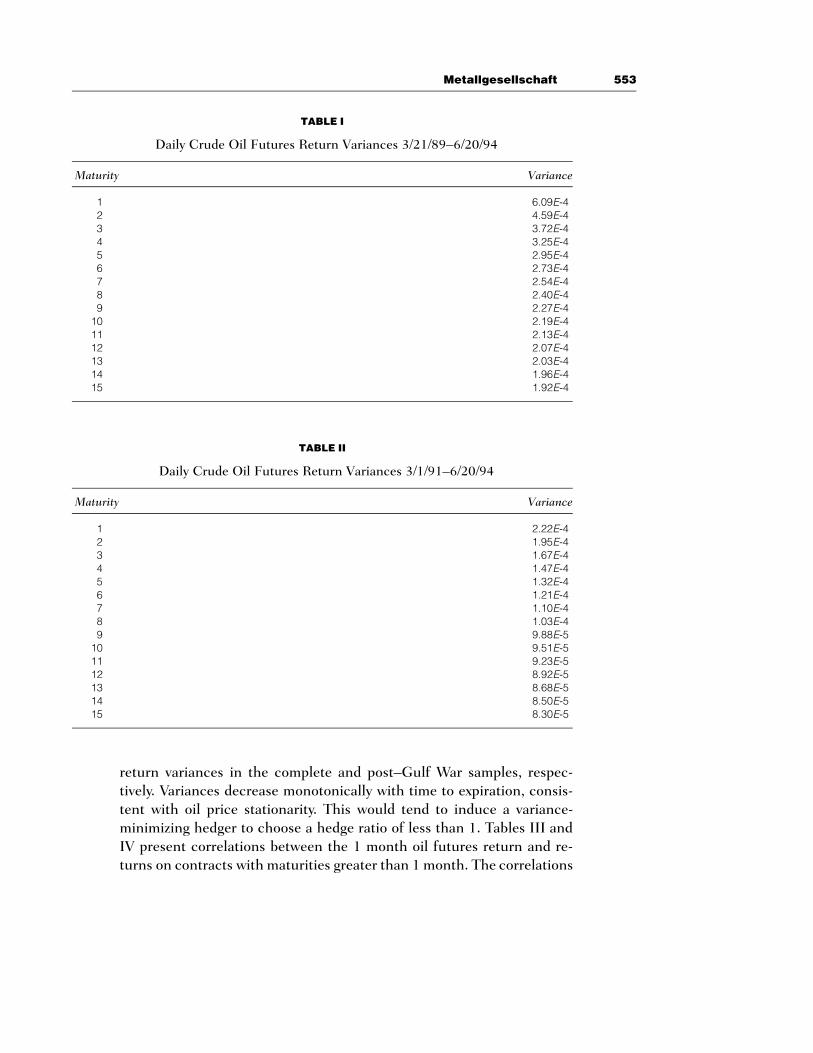
A preliminary analysis of the data also strongly suggests that a one-for-one hedge is not variance minimizing. Tables I and II present futures


TABLE I

Daily Crude Oil Futures Return Variances 3/21/89–6/20/94

Maturity Variance

1 6.09E-42 4.59E-43 3.72E-44 3.25E-45 2.95E-46 2.73E-47 2.54E-48 2.40E-49 2.27E-4

10 2.19E-411 2.13E-412 2.07E-413 2.03E-414 1.96E-415 1.92E-4

TABLE II

Daily Crude Oil Futures Return Variances 3/1/91–6/20/94

Maturity Variance

1 2.22E-42 1.95E-43 1.67E-44 1.47E-45 1.32E-46 1.21E-47 1.10E-48 1.03E-49 9.88E-5

10 9.51E-511 9.23E-512 8.92E-513 8.68E-514 8.50E-515 8.30E-5

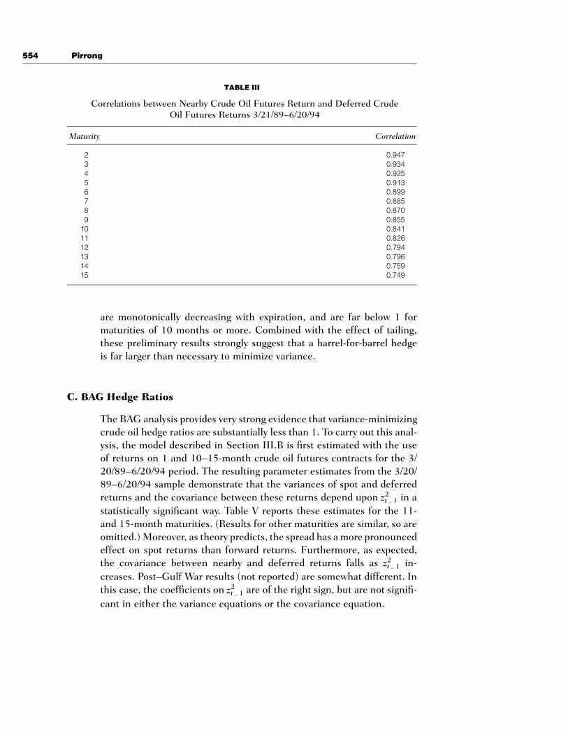
return variances in the complete and post–Gulf War samples, respec-tively. Variances decrease monotonically with time to expiration, consis-tent with oil price stationarity. This would tend to induce a variance-minimizing hedger to choose a hedge ratio of less than 1. Tables III andIV present correlations between the 1 month oil futures return and re-turns on contracts with maturities greater than 1 month. The correlations

554 Pirrong

TABLE III

Correlations between Nearby Crude Oil Futures Return and Deferred CrudeOil Futures Returns 3/21/89–6/20/94

Maturity Correlation

2 0.9473 0.9344 0.9255 0.9136 0.8997 0.8858 0.8709 0.855

10 0.84111 0.82612 0.79413 0.79614 0.75915 0.749

are monotonically decreasing with expiration, and are far below 1 formaturities of 10 months or more. Combined with the effect of tailing,these preliminary results strongly suggest that a barrel-for-barrel hedgeis far larger than necessary to minimize variance.

C. BAG Hedge Ratios

The BAG analysis provides very strong evidence that variance-minimizingcrude oil hedge ratios are substantially less than 1. To carry out this anal-ysis, the model described in Section III.B is first estimated with the useof returns on 1 and 10–15-month crude oil futures contracts for the 3/20/89–6/20/94 period. The resulting parameter estimates from the 3/20/89–6/20/94 sample demonstrate that the variances of spot and deferredreturns and the covariance between these returns depend upon in a2zt 11

statistically significant way. Table V reports these estimates for the 11-and 15-month maturities. (Results for other maturities are similar, so areomitted.) Moreover, as theory predicts, the spread has a more pronouncedeffect on spot returns than forward returns. Furthermore, as expected,the covariance between nearby and deferred returns falls as in-2zt 11

creases. Post–Gulf War results (not reported) are somewhat different. Inthis case, the coefficients on are of the right sign, but are not signifi-2zt 11

cant in either the variance equations or the covariance equation.


TABLE IV

Correlations between Nearby Crude Oil Futures Return and Deferred CrudeOil Futures Returns 3/1/91–6/20/94

Maturity Correlation

2 0.9893 0.9784 0.9675 0.9546 0.9417 0.9228 0.9099 0.896

10 0.88511 0.87512 0.86413 0.85414 0.84515 0.836

To calculate hedge ratios with the BAG model, parameter values areupdated by reestimating the model on a weekly basis. Thus, for hedgeratios for the 7-day period commencing 9/1/92, parameters estimatedover the 3/21/89–8/31/92 period are used. For hedge ratios for the 7-dayperiod commencing 9/8/92, parameters estimated on a 3/21/89–9/7/92sample are used, and so on. This ensures that hedge ratio estimates arebased on information available to MG when it was making its decisions.Using these parameters, the fitted value of the spot return variance andthe spot-deferred return covariances are calculated to determine vari-ance-minimizing hedge ratios.

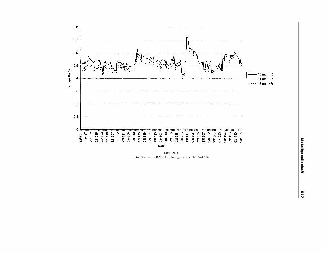
Figure 1 illustrates the variance-minimizing hedge ratios for the 13–15-month maturities over the late 1992–early 1994 period, during whichMG’s hedging strategy was in place. For the September 1992–June 1993period, variance-minimizing hedge ratios were typically less than 0.5 forthese longer times to expiration. For the June–December, 1993 period,hedge ratios ranged between 0.5 and 0.6. Thus, the barrel-for-barrelhedge was not variance increasing for these maturities, but was still con-siderably overhedged. Figure 2 illustrates the variance-minimizing hedgeratios estimated from the post–Gulf War subsample. Although the hedgeratios are somewhat higher than those depicted in Figure 1, they are stillconsistently smaller than 1. In sum these results provide strong evidencethat the barrel-for-barrel strategy did not substantially reduce MG’s risk.

556 Pirrong

TABLE V

Backwardation Adjusted Garch Estimates (T Statistics in Parentheses) 3/21/89–6/20/94

Maturity

11 Months 15 Months

xs 1.0E-6 1.0e-6(0.3460) (0.659)

d1 0.9168 0.9176(83.80) (76.81)

d2 0.0724 0.0726(6.99) (6.29)

d3 9.4E-5 5.6E-5(2.45) (2.01)

xF 1.0E-6 1.0e-6(0.217) (0.364)

f1 0.9125 0.9155(73.94) (68.11)

f2 0.0750 0.0745(6.78) (3.99)

f3 5.0E-5 3.2E-5(2.79) (2.55)

q 0.8343 0.801(53.66) (41.23)

h 12.8E-5 11.16E-4(11.53) (12.48)

H 0.1760 0.1944(12.09) (9.26)

Log L 8329 8186

These inflated hedge ratios increased the variance of MG’s position.To estimate the effects of overhedging on this variance, the fitted vari-ances for the spot and deferred futures returns are used to calculate thevariance of the returns on MG’s positions in the 13–15-month maturities.Formally, this variance is equal to

2 2 2 2r(T t)1 12h 4 (1 1 b ) S h ` (1 1 R ) F e h ,t,T t S,t F,t t,T F,tt

where 4 /hS,thF,t is the squared correlation between the spot2 2R rF,t S,F,t

and futures returns. Figure 3 depicts

2 2r(T t) 2 21 1 2h /[(1 1 R )e F h ] 4 1 ` (1 1 b ) S hF,t t,T F,t t,T t S,tt

2r(T t) 21 12/[(1 1 R )e F h ]t,T F,t

for the September 1992–December 1993 period, where the hedge ratiosand squared correlations are calculated based on the estimates from the

Me

tallg

ese

llsch

aft

55

7

FIGURE 113–15 month BAG CL hedge ratios. 9/92–1/94.

55

8P

irron

g

FIGURE 213–15 month BAG CL hedge ratios. (Gulf War data excluded from estimation)

Me

tallg

ese

llsch

aft

55

9

FIGURE 3Ratio of hedged variance to minimized variance. (Gulf War period excluded from estimation)

560 Pirrong

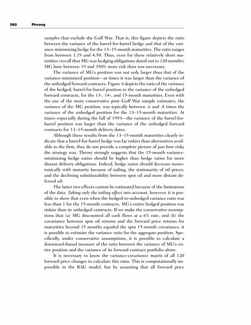
samples that exclude the Gulf War. That is, this figure depicts the ratiobetween the variance of the barrel-for-barrel hedge and that of the vari-ance-minimizing hedge for the 13–15-month maturities. The ratio rangesfrom between 1.19 and 4.50. Thus, even for these relatively short ma-turities (recall that MG was hedging obligations dated out to 120 months)MG bore between 19 and 350% more risk than was necessary.

The variance of MG’s position was not only larger than that of thevariance-minimized position—at times it was larger than the variance ofthe unhedged forward contracts. Figure 4 depicts the ratio of the varianceof the hedged, barrel-for-barrel position to the variance of the unhedgedforward contracts, for the 13-, 14-, and 15-month maturities. Even withthe use of the more conservative post–Gulf War sample estimates, thevariance of the MG position, was typically between .6 and .8 times thevariance of the unhedged position for the 13–15-month maturities. Attimes–especially during the fall of 1993—the variance of the barrel-for-barrel position was larger than the variance of the unhedged forwardcontracts for 13–15-month delivery dates.

Although these results from the 13–15-month maturities clearly in-dicate that a barrel-for-barrel hedge was far riskier than alternatives avail-able to the firm, they do not provide a complete picture of just how riskythe strategy was. Theory strongly suggests that the 15-month variance-minimizing hedge ratios should be higher than hedge ratios for moredistant delivery obligations. Indeed, hedge ratios should decrease mono-tonically with maturity because of tailing, the stationarity of oil prices,and the declining substitutability between spot oil and more distant de-ferred oil.

The latter two effects cannot be estimated because of the limitationsof the data. Taking only the tailing effect into account, however, it is pos-sible to show that even when the hedged-to-unhedged variance ratio wasless than 1 for the 15-month contracts, MG’s entire hedged position wasriskier than its unhedged contracts. If we make the conservative assump-tions that (a) MG discounted all cash flows at a 6% rate, and (b) thecovariance between spot oil returns and the forward price returns formaturities beyond 15 months equaled the spot 15-month covariance, itis possible to estimate the variance ratio for the aggregate position. Spe-cifically, under conservative assumptions, it is possible to calculate adownward-biased measure of the ratio between the variance of MG’s en-tire position and the variance of its forward contract portfolio alone.

It is necessary to know the variance-covariance matrix of all 120forward price changes to calculate this ratio. This is computationally im-possible in the BAG model, but by assuming that all forward price

Me

tallg

ese

llsch

aft

56

1

FIGURE 4Ratio of hedged variance to unhedged variance. (Gulf War period excluded from estimation)

562 Pirrong

changes are perfectly correlated, one can construct an upward-biasedmeasure of the variance of the unhedged position:

120 120ri1 dV 4 var(e DF ) ` 2o t,tìd o oU

i41 i41 j 1?

rj ri 0.51 d 1 d[var(e DF ) var(e DF )] ,t,t`jd t,tìd

where d is 1 month (i.e., 1/12th year). This estimate is biased upwardbecause correlations between different forward prices are in fact less than1. Also, assume that var(DFt,tìd) 4 var(DFt,t`15d) for j . 15. This con-tributes additional upward bias because stationarity causes variances todecline as j increases.

Under the same conservative assumptions, a downward-biased mea-sure of the difference between the variance of MG’s total position (in-cluding long futures and short forwards) and VU equals

120ri1 d2V 4 (120) var(DS ) 1 (2)(120) e cov(DS , DF ),o t,t idH t t `

i 14

where for i $ 15, cov(DSt, DFt,tìd) 4 var(DSt) bt,t`15d. This creates adownward-biased measure of the variance difference because it assumesthat covariances between spot price changes and forward price changesfor more than 15 months to delivery do not decline with time to expirationas theory suggests.

A downward-biased estimate of the ratio of the hedged position var-iance to the unhedged variance equals 1 ` (VH/VU). Despite the down-ward bias of this measure (which may be extreme), the ratio exceeds 1 forall but 8 days in 1993. Indeed, at times this ratio is in excess of 2.5; onOctober 12, 1993, the variance of the hedged position was at least 160%larger than the variance of the unhedged position. On average, during 1993the variance of the hedged position was at least 60% greater than the vari-ance of the unhedged position. Ironically, the variance ratio rose precipi-tously around the same time as MG dramatically increased its positionin September, 1993. In effect, the firm was increasing the size of anincreasingly risky position. Thus, the BAG hedge ratio estimates provideextremely strong evidence that the MG strategy increased, rather thanreduced, the firm’s risk.

In sum, the data provide no support for a barrel-for-barrel hedgingstrategy as a prudent means to synthesize a distant-deferred forward po-sition. The most favorable hedge ratio estimates (from the post–Gulf War


BAG model) imply that the barrel-for-barrel strategy was at least 2–4times riskier than the variance-minimized position. Moreover, extremelyconservative estimates imply that the barrel-for-barrel strategy substan-tially increased the riskiness of MG’s position for virtually all of 1993. Aseverely downwards-biased estimate implies that MG’s hedged positionwas almost always riskier-and sometimes substantially so-than its positionin the delivery contracts alone. Thus, all of the evidence strongly demon-strates that rather than serving to protect the firm against oil price move-ments, MG’s futures trades actually increased the risk for the firm.8

It should also be recognized that in addition to forcing MG to bearmore variance than necessary, the barrel-for-barrel strategy also resultedin substantial kurtosis. The GARCH models all demonstrate that the dis-tribution of oil returns is very fat tailed. The point estimates of H in thesemodels fall around 0.2. Because this parameter estimates the inverse ofthe number of degrees of freedom of the joint distribution of spot andfutures returns, this implies that crude oil returns follow a t distributionwith only 5 degrees of freedom. Thus, the excessive spot crude oil futuresposition (excessive relative to the variance-minimizing position) also im-posed substantially more kurtosis on the firm than was necessary. Risk-averse parties with consistent preferences dislike both variance and kur-tosis (Ingersoll, 1987). Therefore, the barrel-for-barrel hedge was evenmore costly for the firm than the excess variance alone would imply.

It is important to emphasize that the riskiness of the strategy is notprimarily attributable to stacking all positions on the nearby contract. Themaximum variance reduction at any t equals 1 minus the squared cor-relation between spot and forward returns at that t. Setting the squaredcorrelation at t equal to /hS,thF,t (using the daily projected values from2rS,F,t

the BAG and GARCH models) demonstrates that a stacked hedge witha variance-minimizing hedge ratio would have reduced variance for 13–15-month forward positions by between 70 and 80% throughout 1993.Although including deferred futures contracts and longer-term swaps inthe hedge could have reduced risk further, it is certainly possible that theadditional transactions costs attributable to the lower liquidity of thesecontracts would have outweighed the benefits of the additional risk re-

8It should also be noted that the hedge ratios estimated herein for maturities less than 15 monthsare almost certainly conservative estimates of the hedge ratios for maturities extending from 16months to 10 years. First, holding variances and covariances constant, tailing the hedge causes hedgeratios to fall with time to maturity. Second, in the 10–15-month maturity range, both the correlationbetween the spot and deferred futures and the ratio between the deferred futures variance and thespot variance decline as maturity increases. This is consistent with the stationarity of oil prices andthe fact that more distant contracts are progressively poorer substitutes for spot oil. If this trendcontinues as maturities are extended beyond 15 months, this would also induce a fall in hedge ratios.

564 Pirrong

duction.9 Thus, it was not the stacking per se that presented problems.Instead, it was the overhedging of the stack that grossly inflated the riskof MG’s position.

The main effect of MG’s futures strategy was to transform the natureof the risk it faced. Without futures, MG was vulnerable to a rise in thelevel of oil prices. With a futures position that was larger than the vari-ance-minimizing position stacked on the nearby contract, MG was vul-nerable to a steepening of the term structure of crude oil prices. Thefirm’s position hedged against some risks (a parallel shift in the termstructure), but raised its exposure to others (a steepening of this struc-ture). Thus, the strategy embedded both speculative and hedging com-ponents: it speculated on the basis between nearby and deferred oilprices, while hedging against spot oil price changes.

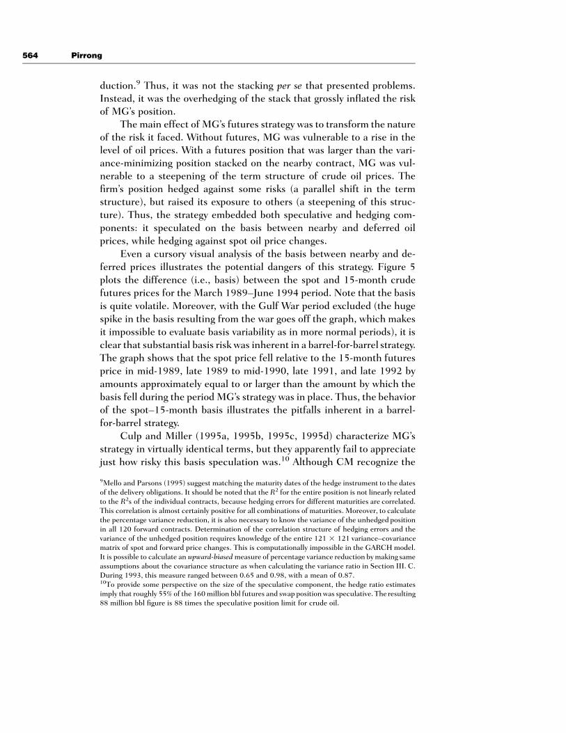
Even a cursory visual analysis of the basis between nearby and de-ferred prices illustrates the potential dangers of this strategy. Figure 5plots the difference (i.e., basis) between the spot and 15-month crudefutures prices for the March 1989–June 1994 period. Note that the basisis quite volatile. Moreover, with the Gulf War period excluded (the hugespike in the basis resulting from the war goes off the graph, which makesit impossible to evaluate basis variability as in more normal periods), it isclear that substantial basis risk was inherent in a barrel-for-barrel strategy.The graph shows that the spot price fell relative to the 15-month futuresprice in mid-1989, late 1989 to mid-1990, late 1991, and late 1992 byamounts approximately equal to or larger than the amount by which thebasis fell during the period MG’s strategy was in place. Thus, the behaviorof the spot–15-month basis illustrates the pitfalls inherent in a barrel-for-barrel strategy.

Culp and Miller (1995a, 1995b, 1995c, 1995d) characterize MG’sstrategy in virtually identical terms, but they apparently fail to appreciatejust how risky this basis speculation was.10 Although CM recognize the

9Mello and Parsons (1995) suggest matching the maturity dates of the hedge instrument to the datesof the delivery obligations. It should be noted that the R2 for the entire position is not linearly relatedto the R2s of the individual contracts, because hedging errors for different maturities are correlated.This correlation is almost certainly positive for all combinations of maturities. Moreover, to calculatethe percentage variance reduction, it is also necessary to know the variance of the unhedged positionin all 120 forward contracts. Determination of the correlation structure of hedging errors and thevariance of the unhedged position requires knowledge of the entire 121 2 121 variance–covariancematrix of spot and forward price changes. This is computationally impossible in the GARCH model.It is possible to calculate an upward-biased measure of percentage variance reduction by making sameassumptions about the covariance structure as when calculating the variance ratio in Section III. C.During 1993, this measure ranged between 0.65 and 0.98, with a mean of 0.87.10To provide some perspective on the size of the speculative component, the hedge ratio estimatesimply that roughly 55% of the 160 million bbl futures and swap position was speculative. Theresulting88 million bbl figure is 88 times the speculative position limit for crude oil.


FIG

UR

E5

Spo

t–15

-mon

thC

Lba

sis.

566 Pirrong

possibility for term structure shifts (which they refer to as “covariancerisk”) they do not quantify the risks these shifts actually create for a firmwith a barrel-for-barrel stacked hedge. They claim (1995d) that the basisrisk inherent in MG’s strategy was so small that it exposed MGRM to noreal threat of bankruptcy whereas naked spot price exposure may wellhave. They justify this assertion by noting that the correlation betweenspot and nearby futures prices is high. This is not the relevant correlation,however. Instead, the correlations between the nearby futures price anddeferred forward prices determine basis risk. All of the empirical resultscontained herein demonstrate conclusively that this correlation is smallenough to make basis risk considerable. Indeed, the evidence implies thatthis basis risk was substantially greater than the risk of the short forwardcontracts alone!

Overhedging also exacerbated the pressures on MG’s liquidity.Whereas its cash market contracts did not impose substantial demandson MG’s cash flows, its futures contracts were marked to market daily.As a result, the firm needed cash to finance margin calls as the nearbyfutures price fell in late 1993. It was the inability to finance these marginflows that forced the firm to seek assistance from its bankers. The liquiditystrains resulting from overhedging could have impaired the efficientoperation of the firm. In the presence of information asymmetries, a fallin liquidity can force a firm to forgo positive NPV projects (Froot, Scharf-stein, and Stein, 1994). Therefore, overhedging was undesirable not onlybecause it exacerbated MG’s solvency risk; the liquidity risk inherent inoverhedging made it even less desirable for the firm to use a barrel-for-barrel strategy. Put differently, whereas the objective function in (11) andthe hedge ratios explicitly consider only solvency, expanding the analysisto include liquidity considerations strengthens the conclusion that barrel-for-barrel hedging was inappropriate.

The barrel-for-barrel strategy was undesirable even if one acceptsCM’s claim that Deutsche Bank and other MG creditors mistook a li-quidity crisis for a solvency crisis, and thus intervened unwisely by forcingthe firm to scale back its oil market activities. Barrel-for-barrel hedgingincreased the likelihood of such a mistaken intervention because it in-creased MG’s liquidity needs. Thus, regardless of whether one examinesliquidity or solvency considerations, barrel-for-barrel hedging was ill-advised.

The results presented in this section provide compelling evidencethat MG’s strategy was highly speculative. It is the most reliable evidencepertaining to this question presented to date. Mello and Parsons (1995)calculate hedge ratios based on the model estimates of Gibson and


Schwartz (1991). Their evidence is somewhat suspect because (as ad-mitted by Gibson and Schwartz) the estimates imply an implausibly highrisk premium in oil futures prices. It is also somewhat dated, as the Gib-son–Schwartz sample period ends 4 years prior to the beginning of MG’sinvolvement in the oil market. Edwards and Canter (1995) use a simpleregression analysis to calculate hedge ratios. This methodology does nottake into account the stochastic nature of volatility and covariances inthe energy market. Moreover, it does not take into account how back-wardation affects variance-minimizing hedge ratios. Thus, the results pre-sented here are based on a more flexible and complete analysis of oil pricedynamics than utilized in previous studies of MG.

Unless one is willing to argue that MG’s managers possessed appre-ciable information advantages regarding future basis movements, it isdifficult to conclude that the barrel-for-barrel strategy was prudent. Ananalysis of the ex post performance of the hedge casts considerable doubtupon the prescience of MG’s managers. The next section addresses thisissue in detail.

V. THE MAGNITUDE OF LOSSESATTRIBUTABLE TO BARREL-FOR-BARRELHEDGING

To determine the gains/losses attributable to barrel-for-barrel hedging,the payoffs to this strategy are estimated with the use of some assump-tions about the size of the cash and futures positions, and the behaviorof the term structure for maturities greater than 15 months. The param-eters necessary to calculate gains/losses, namely, the size and maturity ofthe cash position, are set equal to the public descriptions of MG’s activ-ities. However, because the exact details of MG’s strategy are not known,the simulation results are merely illustrative. It is important to rememberthat the exact details of MG’s cash market, futures market, or swap po-sitions at each relevant date are not known. Moreover, these simulationsdo not take into account the option features of the MG cash marketcontracts. Given these caveats, the simulation results do suggest that abarrel-for-barrel strategy on a 10-year, 160-mm bbl position could haveled to economic losses of upwards of $800,000,000 over the January 2,1993–January 3, 1994 period.

Simulated profits/losses are calculated as follows. It is assumed thatas of 1/2/93 MG was obligated to deliver 107 mm bbl/120 4 893,333 4

bbl of crude oil each month from 1/2/93 to 9/1/2002. To reflect theQ*1increase in MG’s contractual obligations in September, 1993, it is as-

568 Pirrong

sumed that, as of 9/15/93 MG, was obligated to deliver (160 mm 1 7.14mm bbl)/120 4 1,273,777 4 bbl of crude oil in each of the next 120Q*2months; the reduction of 7.14 mm bbl reflects deliveries from Februaryto September, 1993. It is assumed that MG held one barrel in the nearbyfutures contract for each barrel in cash contract delivery commitments.That is, as of 1/2/93, it is assumed that MG was long 107 mm bbl of theFebruary contract, and on 9/15/93 MG they were long 152,853,333 mmbbl of the October contract. On the first business day of each month, thisposition is reduced by barrels to reflect the expiration of a deliveryQ*icommitment, where i 4 1 before 9/15/93, and i 4 2 afterwards.

On each business day, the gain/loss on the nearby futures positionis determined by multiplying the change in the nearby price by the sizeof the nearby futures position. Moreover, on the first business day of eachmonth, the gains on the expiring delivery commitment are calculated asfollows. The per-barrel gain/loss on the first business day is set equal to11 times the difference between the price of the nearby contract andthe price of that month’s contract as of 1/2/93. For example, on February1, 1993, the per barrel gain/loss is set equal to 11 times the differencebetween the March 1993 futures price on that date and the March, 1993futures price as of 1/2/93. This difference is then multiplied by .Q*i

For each business day in the estimation period, the gains/losses onthe long nearby futures position and any expiring delivery commitmentare added to determine a daily gain/loss. In addition, interest on the cu-mulative gain/loss carried over from the previous business day is calcu-lated with the use of the 3-month T-bill rate. Given that MG’s financingcost was larger than the T-bill rate, this is a conservative assumption. Foreach business day t in the sample period, the gain/loss on the nearbyposition, the gain/loss on any expiring delivery commitment, and the netinterest expense at t are then added to the cumulative gain/loss carriedover from t 1 1 to determine the cumulative gain/loss at t.

This process is repeated daily until 1/3/94. On that day, the unexpireddelivery commitments are valued as follows. It is assumed that as of 1/2/93 the forward prices for delivery commitments for all months fromMarch 1994 and beyond are equal to the April 1994 futures price on 1/2/93. That is, as of 1/2/93, the term structure of crude oil prices beyond15 months is assumed flat. Call this price, F1/2/93,15. Similarly, as of9/15/93 the term structure beyond 15 months is flat, with a price,F9/15/93,15. For each month, the difference is calculated between the priceof the futures contract expiring closest to (but after) March 1994 and0.67F1/2/93,15 ` 0.33F9/15/93,15. The averaging reflects that MG enteredinto one-third of its contracts in September, 1993. This difference is then


discounted back to 1/3/94 by the appropriate Treasury rate and multipliedby . For example, for the July 1, 1994 delivery commitment, the dif-Q*2ference is calculated between the August 1994 futures price and0.67F1/2/93,15 ` 0.33F9/15/93,15, this difference is discounted back to 1/3/94 with the use of the 6-month T-bill rate, and this discounted pricedifference is multiplied by .Q*2

To value as of 1/3/94 the forward commitments dated after May1995, it is assumed that the forward prices for these delivery dates equalthe June 1995 futures price. That is, it is assumed that the term structureof crude oil prices for delivery more than 15 months hence is flat as of1/3/94. Call this price, F1/3/94,15. The change in the forward price on thesedelivery commitments over the 1/2/93–1/3/94 period is set equal to0.67F1/2/93,15 ` 0.33F9/15/93,15 1 F1/3/94,15. For each delivery date thisdifference is discounted back to 1/3/94 by the appropriate Treasury rateand multiplied by . For instance, the price difference for the 1/2/96Q*2delivery commitment is discounted with the use of the yield on the 2-year T-note.

The marked-to-market values of these forward commitments on 1/3/94 are added to the cumulative gain/loss on the nearby futures and thegains/losses on the 2/1/93–12/1/93 delivery commitments to calculate thecumulative gain/loss on the entire MG position over the 1/2/93–1/3/94period. Because all outstanding forward commitments are marked to mar-ket, the resulting total is an estimate of the economic gain/loss of a barrel-for-barrel strategy.

This methodology implies that the losses on a barrel-for-barrel strat-egy over the 1/2/93–1/3/94 period were equal to approximately$800,000,000. This is due to a loss of $1,090,000,000 on crude oil fu-tures and expired delivery commitments and a gain of about$290,000,000 on unexpired delivery commitments. If MG had used var-iance-minimizing hedge ratios rather than a barrel-for-barrel futures po-sition throughout the period, their losses would have fallen by almost78%, to only $181,000,000. To derive this estimate, variance-minimizinghedge ratios are based on the post-War BAG estimates. Ratios for ma-turities in excess of 15 months are set equal to the 15-month hedge ratiomultiplied by the relevant tailing factor. For example, on each day the 24-month hedge ratio is set equal to the 15-month hedge ratio multiplied bythe discount factor relevant between month 15 and month 24. Becausethis almost certainly leads to upward-biased estimates of variance-mini-mizing hedge ratios for delivery commitments 16 months and more intothe future, the loss estimate of $181,000,000 is biased upwards as well.

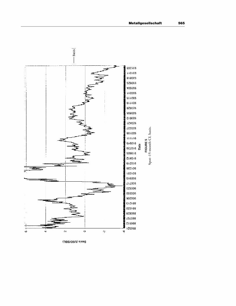
57

0P

irron

g

FIGURE 6MG’s 1993 losses.


Figure 6 illustrates how these losses grew over the course of 1993.Prices actually moved in MG’s favor in the first five months of 1993, andthe firm profited accordingly. In June and in subsequent months, however,the term structure steepened appreciably; MG’s ballooning losses duringthis period reflect these price movements.

It is interesting to note that these losses are comparable to thosepresented in an audit by the German accounting firms C&L TreuarbeitDeutsche Revision and Wollert-Elmendorff Industrie Treuhand. Basedon an analysis of MGRM’s accounting data, these firms report a grossloss on the futures and forward positions of $1.277 billion, and a gain of$245 million on the unexpired delivery commitments, for a net loss of$1.06 billion. (The residual is attributable to losses on firm-flexible con-tracts not considered in this study.)

It should also be noted that if liquidity shortages imposed costs uponthe firm, or made mistaken intervention by creditors more likely (as pos-ited by CM) the marked-to-market losses do not reveal the full scope ofMG’s problems. The roughly $1.1 billion loss on the futures position (netof gains on expired delivery commitments) represents the immediate de-mand on MG’s cash flows. If the firm had used a variance-minimizinghedge ratio (that is, if it minimized solvency risk), its cash outflows underthe hedging program would have equaled only $.471 billion—about 57%less than the loss actually realized. Thus, if liquidity strains reduce firmvalue, the $800 million marked-to-market loss understates the costs ofbarrel-for-barrel hedging because the firm also incurred costs attributableto the extra liquidity drains attributable to overhedging.

The large losses quantified here underscore the speculative natureof MG’s strategy, and cast doubt upon the prescience of its managers.Although even the most well informed market participants lose money attimes, the magnitude of the losses realized in 1993 strongly suggests thatMG’s management did not possess so acute an ability to forecast basismovements to justify the immense risks inherent in their strategy.

VI. THE EFFECTS OF EMBEDDED OPTIONSON HEDGE RATIOS

The preceding analysis calculates hedge ratios under the assumption thatMG’s forward contracts did not embed any options. Recall, however, thatthe firm-fixed supply contracts did permit the buyers to terminate theircontracts and, upon said termination, receive one-half of the differencebetween the prevailing spot price (measured by the nearby futures price)and the fixed price established in the contract times the volume remaining

572 Pirrong

under the contract. Formally, if a customer were to exercise this optionat time t, he or she would receive 0.5Q(St 1 f), where f is the fixed priceunder the contract, Q is the volume remaining under the contract, and(as before) St is the spot price. Upon exercise, the customer would ter-minate his right to receive refined products at the fixed price for theremaining life of the contract.

CM claim that this feature of the MG contracts made it even moredesirable to use nearby futures contracts to hedge the energy price riskinherent in the supply contracts. They state that “MGRM could liquidatean equivalent amount of futures positions to cover the required cashoutlay. Because both the hedge and the early exercise option relied uponthe front-month futures contract, the price in MGRM’s hedge was thesame as that governing early termination options. MGRM therefore facedno covariance risk . . . from the risk of early exercise.”

In reality, the effect of the embedded option is much more compli-cated; it could have either exacerbated or mitigated the overhedging prob-lem. In essence, it is necessary to account for the fact that oil pricechanges also affect the value of the forward contracts that customerswould forfeit when exercising the option. When this factor is taken intoaccount, the values of the early-out option and the position necessary tohedge it both depend upon the entire term structure of oil prices.

From MG’s perspective, the firm-fixed contracts were equivalent toa portfolio consisting of a receive fixed-pay floating energy swap and ashort position in a call option on this swap. There are N delivery monthsremaining on the swap, and MG must deliver Q/N units of petroleumproducts on each delivery date. Call Zt the value of the swap to MG attime t. That is,

N Qri1 dZ 4 e ( f 1 F ).o t,t`idt N4i 1

As before, Ft,t`id gives the forward price for delivery at t ` id as of t, andd equals 1 month (i.e., 1/12 of a year). The value of the swap to MG’scustomers (i.e., its counterparties) is 1Zt.

If the customer exercises the option embedded in the MG contracts,he or she receives

0.5(S 1 f )Q 1 (1Z ) 4 0.5(S 1 f )Q ` Z [ A .t t t i t

The 1(1Zt) term enters the expression because, upon exercising theoption, the customer gives up his swap position, which is worth 1Zt tohim.


Define q(At, T,t), the value of the option to terminate the contractand receive a payment of 0.5(St 1 f )Q as a function of At, the endingdate on the contract, and the current date. This option is a call on theportfolio At, with a strike price of 0. Then, the value of MG’s position attime t is

P 4 Z 1 q(A , T,t). (6)t t

To determine how many nearby futures contracts to purchase to hedgethis obligation, first recognize that

]P ]Z ]q(A , T,t)t t4 1 13 4]F ]F ]At,tìd t,tìd t

Q ]q(A , T,t) Qri1 d t41e 1 1 [ D (t,t ` id) . 1 .3 4 FN ]A Nt

The inequality follows because the option increases in value as At in-creases (i.e., ]q/]At . 0). Moreover,

]P ]q(A , T,t) ]A ]q(A , T,t)t t t4 1 4 1 0.5Q [ D , 0.S]S ]A ]S ]At t t t

If only the nearby contract is used to hedge, the total number of nearbycontracts to buy to hedge the entire swap and embedded option is

NridH [ 1 [e D (t,t ` id) b ] 1 Do t,tìdT F S

i41

N Q ]q ]q4 b 1 1 ` 0.5 .o t,tìd3 1 2 4N ]A ]Ai41 t t

This may be either larger or smaller than the total number of nearbycontracts required to hedge the swap alone, depending on whether theaverage hedge ratio (absent the option) is less than or greater than 0.5.Recall that a position is variance increasing if it is more than twice aslarge as the total variance-minimizing hedge. The barrel-for-barrel strat-egy is thus risk increasing in the absence of the embedded option if

N Qb , 0.5Qo t,tìdNi41

If this expression holds, rewriting HT implies

574 Pirrong

N]q Q ]q ]q

H 4 1 1 b ` 0.5Q , 1 1 0.5Qo t,t`id1 2 1 2T ]A N ]A ]Ai41t t t

]q` 0.5Q 4 0.5Q.

]At

Therefore, if the barrel-for-barrel position increases variance in the ab-sence of the embedded option, it increases the variance if the contractincludes the option as well. The option feature mitigates the overhedgingsomewhat, but not enough to turn the barrel-for-barrel strategy into atrue hedge.

In sum, the analysis of this section demonstrates that the optionsembedded explicitly in MG’s firm-fixed contracts cannot reverse, and maystrengthen, the conclusions drawn in the previous sections. Because theempirical results presented earlier demonstrate that buying nearby con-tracts barrel-for-barrel resulted in substantial overhedging in the absenceof these options, the option analysis strengthens the conclusion that MG’sstrategy almost certainly increased the variance of the firm’s payoffs.

The options embedded in the firm-flexible contracts are more diffi-cult to analyze than those in the firm-fixed deals. The 15-month hedgeratios estimated earlier are likely to provide an upper bound on the hedgeratios for delivery commitments 2 years and beyond even in the presenceof this option, however. The drop in oil prices (combined with the meanreversion in oil prices) during the life of the program gave buyers a strongincentive to defer, rather than accelerate, deliveries. Because more distantdeliveries require smaller hedge ratios, this bias towards deferral suggeststhat the no-option hedge ratios overestimate the with-option hedge ratiosfor firm-flexible contracts as well.

VII. ROLLOVER PROFITS AND THEPRUDENCE OF THE BARREL-FOR-BARRELHEDGE

It has been argued that MG’s policy allowed the firm to profit from thebackwardation typical in energy markets by rolling over its futures at aprofit. That is, when the market is in backwardation, at the expirationdate of each contract the firm could expect to sell the expiring future ata price that exceeded that at which it purchased the next-to-expire con-tract. Arthur Benson, the main architect of MG’s strategy, apparentlyrelied upon such reasoning (Benson Affidavit, 1994). Edwards and Can-ter (1995, p. 224) state that “it does not seem unreasonable for MGRMto have expected that over a long period of time (such as ten years) its


hedging strategy would have produced a net rollover gain.” Edwards andCanter, however, recognize that there were appreciable risks in such astrategy.

An analysis of this argument reveals that the expected gain fromrolling over nearby futures for K periods in a market that is in backwar-dation is equal to the current difference between the spot price of oil andthe K-period forward price. If each successive nearby futures price isexpected to exceed the next expiring futures price for K consecutivemonths, the sum of these differences equals the difference between thecurrent spot price and the K-month futures price. As a result, in a driftlessfutures market, the expected cost of oil incurred in a rollover strategyending in month K equals the current forward price of oil for delivery inmonth K. This strategy is riskier than the variance-minimized replicationof the K-month forward contract, however, so it is dominated by thatstrategy.

These points are readily grasped by expressing the firm’s cost of ac-quiring oil to satisfy its contractual obligation (denoted by C) to deliveroil in K months as follows:

K

C 4 S 1 [F 1 F ] 4 S ` F 1 Fo i,i i11,i 0,1 K,KK Ki41

K 11

` [F 1 F ].o i,i`1 i,ii41

Here Fi,j is the forward price of oil in month i for delivery in month j,and SK is the spot price of oil in month K. For simplicity, this expressionassumes that the interest rate equals 0, which simplifies the notation buthas no effect on the results. In this expression, the total cost equals thespot price of oil in month K 1 SK—minus the total realized rollover gainson futures contracts. The summation term is the total rollover gain, wherein month i the rollover gain is defined as the deferred price minus theexpiring price, Fi,i`1 1 Fi,i. With driftless futures prices, this expressionimplies that E0(C) 4 E0(SK) 4 F0,K. Also note that the convergence ofspot and futures implies SK 4 FK,K. Therefore,

K 11

E (C) 4 E F 1 [F 1 F ] 4 F .0,1 o i,i`1 i,i 0,K5 60 0i41

Because F0,1 equals the price of acquiring oil 1 month after the initiationof the strategy, this expression states that the 1 month forward price netof the rollover gains expected over K month equals the K-period forward

576 Pirrong

price of oil. In essence, the expected rollover gains reduce the expectedcost of acquiring oil for delivery in K months below the current spot priceof oil. But in a market in backwardation, the K-month forward price isalso below the current spot price by the same amount. That is, the ex-pected total rollover gain equals the amount of backwardation over Kmonths. The barrel-for-barrel rollover strategy is riskier than the variance-minimizing replication of the K-period forward price, however. Thus,there were less-risky ways for MG to exploit the backwardation in themarket than a barrel-for-barrel rollover every month.

VIII. SUMMARY AND CONCLUSIONS

A thorough analysis of the behavior of oil prices demonstrates clearly thatMGRM’s strategy of purchasing one barrel of spot crude oil to hedge thesale of crude oil months into the future was almost certainly risk increas-ing, rather than risk reducing. The reasons for this are clear. First, thestationarity of oil prices implies that volatilities decline systematicallywith time to expiration. Second, the correlation between spot and de-ferred prices is imperfect, and this correlation also declines systematicallyas time to expiration of the deferred increases. A variance-minimizinghedger should reduce hedge ratios far below 1 in response to these fac-tors: MG did not.

Empirical estimates provide extremely compelling evidence that, dueto this overhedging, MG’s position of long futures and short forwards wassubstantially riskier than its short position in forward contracts alone.Therefore, this strategy subjected the firm to the risk of real economicloss, not just accounting loss. The firm was vulnerable to a steepening ofthe oil price term structure, an event that occurred soon after it imple-mented its strategy. A simulation of the economic losses a firm employingsuch a strategy would have incurred produces figures that are comparableto the magnitude of the losses publicly recognized by MG. Thus, the dataprovide compelling evidence that MG’s strategy imposed substantial riskupon the firm ex ante, and that the ex post losses were substantial.

This is not to say that all firms should employ variance-minimizinghedges when trading derivatives: informed speculation is a common partof any risk-management strategy. The relevant question is whether MGpossessed the information advantage required to justify its immense spec-ulative position. There is substantial reason to doubt that any firm, letalone a relative newcomer to the energy markets like MG, has a largeenough informational advantage to justify the immense risks of what wasarguably the largest time spread ever undertaken in commodity markets.


The losses incurred in the last half of 1993 certainly cast significant doubtupon the firm’s ability to predict the movements of oil prices. Given thehuge losses incurred in late 1993, a Bayesian estimating the probabilitydistribution of MG’s information advantage would almost certainly placelittle weight on the possibility that the firm was well informed, and greatweight on the possibility that it did not possess superior information,regardless of the charitability of his priors concerning the prescience ofMG’s managers.

APPENDIX

If the futures prices are martingales, then .22E [P 1 E P ] 4 E Pt t t T0 0 0T TConsider the determination of the first hedge ratio ( ) in a dynamicbt t,T0`D

hedge that accounts for possible dependencies between hedge ratios atany time t and hedge ratios at subsequent times t8 . t. The relevant first-order condition is

2dE Pt T0 24 0 4 2E {b DS 1 DS Dvt t t t t t t t t,T0 0 0 0 0`D `D `D `Ddbt t0`D

M

` DS [b DS 1 Dv ]}.t t o t i t,T t i t t i, t,T0 0 0 0`D ` D ` D ` Di 24

The first two terms in this expression are present in a single-period vari-ance-minimizing hedge ratio. The product of the first period spot pricechange and the sum of gains and losses in subsequent periods reflectsthe possible intertemporal dependencies among hedge ratios. Consider arepresentative term:

E [DS b DS ].t t t t i t,T t i t0 0 0 0`D ` D ` D

The hedge ratio at t0 ` i Dt may depend upon previous realizations ofDSt and Dtt,T. However, by the law of iterated expectations:

E [DS b DS ]t t t t i t,T t i t0 0 0 0`D ` D ` D

4 E {DS b [E (DS )]},t t t t i t,T t (i11) t t i t0 0 0 0 0`D ` D ` D ` D

where the inner expectation is conditional on all price changes up to t0` (i 1 1) Dt. Because St is a martingale by assumption, this inner ex-pectation is 0, the entire expression equals 0. Therefore, this expressiondisappears from the first-order condition, as do all other terms includedin the summation. Consequently, the hedge ratio produced as the solutionto the dynamic programming problem collapses to the single-period hedge

578 Pirrong

ratio. It is possible to demonstrate that this result obtains for t . t0 aswell.

BIBLIOGRAPHYAnderson, R., and Danthine, J. (1981): “Cross-Hedging,” Journal of Political Eco-

nomics, 89:1182–1196.Benson, A., (1994): “Affidavit of W. Arthur Benson v. Metallgesellschaft Corp

(and others),” USDC of Maryland, Civil Action JFM-94-484.Chan, A. (1992): “Optimal Dynamic Hedging Strategies with Financial Futures

Contracts Using Nonlinear Conditional Heteroskedasticity Models,” un-published doctoral dissertation, Michigan Business School.

Cox, J., Ingersoll, J., and Ross, S. (1981): “The Relationship between ForwardPrices and Futures Prices,” Journal of Financial Economics, 9:321–346.

Culp, C., and Miller, M. (1994): “Hedging a Flow of Commodity Deliveries withFutures: Lessons from Metallgesellschaft,” Derivatives Quarterly, 1:7–15.

Culp, C., and Miller M. (1995a): “Metallgesselschaft and the Economics of Syn-thetic Storage,” Journal of Applied Corporate Finance, 7:62–76.

Culp, C., and Miller M. (1995b): “Auditing the Auditors,” Risk, 8(4):36–40.Culp, C., and Miller M. (1995c): “Letter to the Editor,” Risk, 8(6):8.Culp, C., and Miller M. (1995d): “Hedging in the Theory of Corporate Finance:

A Reply to Our Critics,” Journal of Applied corporate Finance, 8:121–127.Dixit, A., and Pindyck, R. (1994): Investment under Uncertainty. Princeton, NJ:

Princeton University Press.Duffie, D., and Jackson (1991): “Optimal Hedging and Equilibrium in a Dynamic

Futures Market,” Journal Economic Dynamics and Control, 14:21–33.Edwards, F., and Canter M. (1995): “The Collapse of Metallgesellschaft: Un-

hedgeable Risks, Poor Hedging Strategy, or Just Bad Luck?” Journal of Fu-tures Markets, 15:211–264.

Froot, K., Scharfstein, D., and Stein, J. (1994): “Risk Management: CoordinatingCorporate Investment and Financing Policies,” Journal of Finance,48:1629–1658.

Gibson, R., and Schwartz, E. (1991): “Stochastic Convenience Yield and thePricing of Oil Contingent Claims,” Journal of Finance, 45: 959–976.

Hsieh, D. (1989): “Testing for Nonlinear Dependence in Daily Foreign ExchangeRates,” Journal of Business, 62:339–368.

Ingersoll, J., (1987): Theory of Financial Decision Making. Totowa, NJ: Rowman& Littlefield.

Kroner, K., and Sultan, J. (1991): “Foreign Currency Futures and Time VaryingHedge Ratios,” Pacific-Basin Capital Market Research, 2.

Lien, D., and Luo, X. (1994): “Multiperiod Hedging in the Presence of Condi-tional Heteroskedasticity,” Journal Futures Markets, 14:927–955.

Mello, A., and Parsons, J. (1995): “The Maturity Structure of a Hedge Matters:Lessons from the Metallgesellschaft Debacle,” Journal of Applied CorporateFinance, 8:106–120.

Ng, V., and Pirrong, C. (1994): “Fundamentals and Volatility: Storage, Spreads,and the Dynamics of Metals Prices,” Journal of Business, 67:203–230.

Working, H., (1962): “New Concepts Concerning Futures Markets and Prices,”American Economic Review, 52:248–253.

Metallgesellschaft: A Prudent Hedger Ruined or a Wildcatter on NYMEX?

Documents

Transcript of Metallgesellschaft: A Prudent Hedger Ruined or a Wildcatter on NYMEX?