Metagenomics Workshop SciLifeLabDocumentation

Release 1.0

Johannes Alneberg, John Sundh, Ino de Bruijn, Luisa Hugerth, Anders Andersson

March 01, 2017

Contents

1 Introduction 3

2 Connecting to UPPMAX 52.1 Connecting to UPPMAX . . . . . . . . . . . . . . . . . . . . . . . . . . . . . . . . . . . . . . . . . 52.2 Getting a node of your own . . . . . . . . . . . . . . . . . . . . . . . . . . . . . . . . . . . . . . . 52.3 Load virtual environment . . . . . . . . . . . . . . . . . . . . . . . . . . . . . . . . . . . . . . . . 62.4 Set sample variables . . . . . . . . . . . . . . . . . . . . . . . . . . . . . . . . . . . . . . . . . . . 6

3 Checking required software 73.1 Programs used in this workshop . . . . . . . . . . . . . . . . . . . . . . . . . . . . . . . . . . . . . 73.2 Using which to locate a program . . . . . . . . . . . . . . . . . . . . . . . . . . . . . . . . . . . . . 73.3 Check all programs in one go with which . . . . . . . . . . . . . . . . . . . . . . . . . . . . . . . . 83.4 (Optional excercise) Install sickle by yourself . . . . . . . . . . . . . . . . . . . . . . . . . . . . . . 8

4 Quality Control 114.1 Quality Control with FastQC . . . . . . . . . . . . . . . . . . . . . . . . . . . . . . . . . . . . . . . 114.2 Optional: Quality trimming Illumina paired-end reads . . . . . . . . . . . . . . . . . . . . . . . . . 12

5 Community analysis using 16S reads 155.1 Community analysis using rRNA gene reads . . . . . . . . . . . . . . . . . . . . . . . . . . . . . . 15

6 Metagenomic Assembly 176.1 Assembling reads . . . . . . . . . . . . . . . . . . . . . . . . . . . . . . . . . . . . . . . . . . . . . 17

7 Annotation 217.1 Functional Annotation . . . . . . . . . . . . . . . . . . . . . . . . . . . . . . . . . . . . . . . . . . 217.2 Taxonomic annotation . . . . . . . . . . . . . . . . . . . . . . . . . . . . . . . . . . . . . . . . . . 237.3 Mapping reads and quantifying genes . . . . . . . . . . . . . . . . . . . . . . . . . . . . . . . . . . 257.4 Summarize and explore the annotation . . . . . . . . . . . . . . . . . . . . . . . . . . . . . . . . . 27

i

ii

Metagenomics Workshop SciLifeLab Documentation, Release 1.0

This is a one day metagenomics workshop. We will discuss quality checking, assembly, taxonomic classification,binning and annotation of metagenomic samples. The workshop is developed by the Environmental Genomics groupat KTH / SciLifeLab.

Here is a link to the official homepage for the SciLifeLab workshop in metagenomics.

A presentation for this workshop is available here.

Program:

• Getting started

– Introduction

– Connecting to UPPMAX

– Checking required software

• Sessions

– Quality Control

– Community analysis using 16S reads

– Metagenomic Assembly

– Annotation

Contents:

Contents 1

Metagenomics Workshop SciLifeLab Documentation, Release 1.0

2 Contents

CHAPTER 1

Introduction

In this workshop we will be working with human associated metagenomes from the human microbiome project (HMP),following all the bioinformatic steps beginning with read sequence quality checking and ending with functional anno-tation of assembled contigs. You will be asked to choose one dataset to work with throughout the entire workshop andin the end we will compare results among different groups. The three datasets you can choose from is:

• Skin metagenome

• Tooth metagenome

• Gut metagenome

3

Metagenomics Workshop SciLifeLab Documentation, Release 1.0

4 Chapter 1. Introduction

CHAPTER 2

Connecting to UPPMAX

IMPORTANT: If it happens that you are logged out from your Uppmax session during the course (for instance duringlunch) you need to rerun all of the commands following on this page, except the salloc command.

Connecting to UPPMAX

The first step of this lab is to open a ssh connection to the computer cluster Milou on UPPMAX. If you have a Mac ora PC running Linux, start the terminal (black screen icon). If you work on a PC running Windows, download and startMobaXterm (http://mobaxterm.mobatek.net). Now type (change username to your own username):

ssh -X username@milou.uppmax.uu.se

and give your password when prompted. As you type the password, nothing will show on screen. No stars, no dots.It is supposed to be that way. Just type the password and press enter, it will be fine. You should now get a welcomingmessage from Uppmax to show that you have successfully logged in.

Getting a node of your own

Usually you would do most of the work in this lab directly on one of the login nodes at uppmax, but we have arrangedfor you to have half of one node (=8 cores) each to avoid disturbances. To get this reservation you need to use thesalloc command like this:

salloc -A g2015028 -t 08:00:00 -p core -n 8 --no-shell --reservation=g2015028_1 &

Now check which node you got (replace username with your uppmax user name) like this:

squeue -u username

The nodelist column gives you the name of the node that has been reserved for you (starts with “m”). Connect to thatnode using:

ssh -X nodename

Note: there is a uppmax specific tool called jobinfo that supplies the same kind of information as squeue that you canuse as well ( $ jobinfo -u username). You are now logged in to your reserved node, and there is no need for you to usethe SLURM queuing system. You can now continue with the specific exercise instructions.

5

Metagenomics Workshop SciLifeLab Documentation, Release 1.0

Load virtual environment

We have already installed all programs for you, all you have to do is load the virtual environment for this workshop.Once you are logged in to the server run:

source /sw/courses/metagenomicsAndSingleCellAnalysis/metagenomics/virtenv/bin/activate

If you would have to, you deactivate the virtual environment with the command deactivate, but you don’t have to dothat yet.

NOTE: This is a python virtual environment. The binary folder of the virtual environment has symbolic links to allprograms used in this workshop so you should be able to run those without problems.

Set sample variables

You will now have to make your decision on which kind of dataset you want to work with during this workshop. Thechoices you have are three different sampling sites on or within the human body:

• Gut

• Skin

• Teeth

Run only *one* of the following commands in the terminal

This will set the SAMPLE and SAMPLE_ID variables that will be used in the commands in the next steps of thetutorial. If for some reason you have to restart the terminal you will have to set these variable names again.

Gut

SAMPLE=gutSAMPLE_ID=SRS011405

Teeth

SAMPLE=teethSAMPLE_ID=SRS014690

Skin

SAMPLE=skinSAMPLE_ID=SRS015381

After you have chosen a sample you will create the file structure continuously throughout the workshop. This willmake it possible for us to only use ‘$SAMPLE’ in the commands, and it will automatically be changed to the sampletype that you chose.

6 Chapter 2. Connecting to UPPMAX

CHAPTER 3

Checking required software

An often occuring theme in bioinformatics is installing software. Here we wil go over some steps to help you checkwhether you actually have the right software installed. There’s an optional excerise on how to install the qualitytrimmer sickle.

Programs used in this workshop

The following programs are used in this workshop:

• Bowtie2

• Velvet

• samtools

• Picard

• Diamond

• Megan

• Fastqc

• Sortmerna

• Rdp_Classifier

• Krona

• Prokka

• MinPath

• BedTools

Using which to locate a program

An easy way to determine whether you have have a certain program installed is by typing:

which programname

where programname is the name of the program you want to use. The program which searches all directories in$PATH for the executable file programname and returns the path of the first found hit. This is exactly what happens

7

Metagenomics Workshop SciLifeLab Documentation, Release 1.0

when you would just type programname on the command line, but then programname is also executed. To seewhat your $PATH looks like, simply echo it:

echo $PATH

For more information on the $PATH variable see this link: http://www.linfo.org/path_env_var.html.

Check all programs in one go with which

To check whether you have all programs installed in one go, you can use which. In order to do so we will iterateover all the programs and call which on each of them. First make a variable containing all programs separated bywhitespace:

req_progs="bowtie2 bowtie2-build velveth velvetg parallel samtools interleave-reads.py diamond MEGAN fastqc sortmerna prokka MinPath1.2.py bedtools"echo $req_progs

Now iterate over the variable req_progs and call which:

for p in $req_progs; do which $p || echo $p not in PATH; done

In Unix-like systems a program that sucessfully completes it tasks should return a zero exit status. For the programwhich that is the case if the program is found. The || character does not mean pipe the output onward as you areprobably familiar with (otherwise see http://tldp.org/HOWTO/Bash-Prog-Intro-HOWTO-4.html), but checks whetherthe program before it exists succesfully and executes the part behind it if not.

If any of the installed programs is missing, try to install them yourself or ask. If you are having troubles followingthese examples, try to find some bash tutorials online next time you have some time to kill. Educating yourself on howto use the command line effectively increases your productivity immensely.

Some bash resources:

• Excellent bash tutorial http://tldp.org/HOWTO/Bash-Prog-Intro-HOWTO.html

• Blog post on pipes for NGS http://www.vincebuffalo.com/2013/08/08/the-mighty-named-pipe.html

• Using bash and GNU parallel for NGS http://bit.ly/gwbash

(Optional excercise) Install sickle by yourself

Follow these steps only if you want to install sickle by yourself.

From the sickle project description: “Sickle is a tool that uses sliding windows along with quality and length thresholdsto determine when quality is sufficiently low to trim the 3’-end of reads and also determines when the quality issufficiently high enough to trim the 5’-end of reads. It will also discard reads based upon the length threshold.”

Installation procedures of research software often follow the same pattern, so it’s useful to learn how to do this.Download the code, compile it and copy the binary to a location in your $PATH. The code for sickle is onhttps://github.com/najoshi/sickle. I prefer compiling my programs in ~/src and then copying the resulting programto my ~/bin directory, which is in my $PATH. This should get you a long way:

mkdir -p ~/src

# Go to the source directory and clone the sickle repositorycd ~/srcgit clone https://github.com/najoshi/sicklecd sickle

8 Chapter 3. Checking required software

Metagenomics Workshop SciLifeLab Documentation, Release 1.0

# Compile the programmake

# Create a bin directorymkdir -p ~/bincp sickle ~/bin

3.4. (Optional excercise) Install sickle by yourself 9

Metagenomics Workshop SciLifeLab Documentation, Release 1.0

10 Chapter 3. Checking required software

CHAPTER 4

Quality Control

The first step of any sequencing project is to do quality control of your reads and remove (trim) low quality bases fromthe end of the read. In this exercise, you will work with Illumina data from the Human Microbiome Project that hasalready been trimmed. We still want to check the quality of reads, though.

In this part of the metagenomics workshop we will learn how to:

• Check the quality of your raw sequencing data

• Perform quality trimming using sickle

The workshop has the following exercises:

Quality Control with FastQC

In this excercise you will use FastQC to investigate the quality of your sequences using a nice graphical summaryoutput.

Retrieving your data

For the first step, make a workshop folder in your home directory and move into it:

mkdir -p ~/mg-workshopcd ~/mg-workshop

Inside it, make a folder for your input files:

mkdir -p ~/mg-workshop/data/$SAMPLE/reads/1M/cd ~/mg-workshop/data/$SAMPLE/

Now make a copy of the files you want to work on: gut, skin or teeth datasets. These files were originally taken fromthe Human Microbiome Project and then subsampled to include only 1 million reads each. You can copy these filesfrom the project directory:

cp /sw/courses/metagenomicsAndSingleCellAnalysis/nobackup/metagenomics-workshop/data/$SAMPLE/reads/1M/${SAMPLE_ID}_1M.1.fastq ~/mg-workshop/data/$SAMPLE/reads/1M/cp /sw/courses/metagenomicsAndSingleCellAnalysis/nobackup/metagenomics-workshop/data/$SAMPLE/reads/1M/${SAMPLE_ID}_1M.2.fastq ~/mg-workshop/data/$SAMPLE/reads/1M/

You will now have two files in your reads directory: one for the forward reads *_1.fastq and one for the reversereads *_2.fastq.

11

Metagenomics Workshop SciLifeLab Documentation, Release 1.0

FastQC

We will now use FastQC to generate a report about the quality of our sequencing reads. For most programs and scriptsin this workshop, you can see their instructions by typing their name in the terminal followed by the flag -h. There aremany options available, and we’ll show you only a few of those.

First, make a folder to keep your quality control results:

mkdir -p ~/mg-workshop/results/quality_check/$SAMPLE/

Now, run fastqc for each file:

fastqc -o ~/mg-workshop/results/quality_check/$SAMPLE/ --nogroup ~/mg-workshop/data/$SAMPLE/reads/1M/${SAMPLE_ID}_1M.1.fastq ~/mg-workshop/data/$SAMPLE/reads/1M/${SAMPLE_ID}_1M.2.fastq

FastQC will generate two files for each input file, one compressed, and one not. To view your files, copy the htmlresults into your local computer and open them with a browser.

From your own shell (not inside Uppmax - open a new terminal window):

mkdir -p ~/mg-workshop/cd ~/mg-workshop/scp -r username@milou.uppmax.uu.se:~/mg-workshop/results/quality_check/*/*html .

Instead of username, type your own username!

Now open the reports. Make sure you understand the results. Do they look ok? Is there a difference between forwardand reverse? Are there any warnings or errors? What do they mean? Do you have adapter sequences in your reads?The FastQC project includes an ugly, but useful, tutorial.

Optional: Quality trimming Illumina paired-end reads

In this excercise you will learn how to quality trim Illumina paired-end reads. Illumna paired-end reads are by farthe most common Next Generation Sequencing (NGS) approach for metagenomics. The reads downloaded from theHMP are already quality trimmed. However, if you have time and want to try it out for yourself, you can run somemore stringent quality trimming on them and see what happens.

Running sickle on a paired-end library

For quality trimming Illumina paired end reads we use the library sickle which trims reads from 5’ end to 3’ end usinga sliding window. If the mean quality of bases inside a window drops below a specified number, the remaining of theread will be trimmed.

As a default, sickle trims a read at the point needed to maintain its average quality over 20. It also discards reads thatare shorter than 20 bp. These are very good default values, but in this extra exercise you’re welcome to change thevalues of these parameters using the -q and -l flags.

You can use the same qc directory as before for this step, since these reads won’t be further processed.

Make sure you understand the input parameters and then run sickle,:

mkdir -p ~/mg-workshop/results/quality_check/sickle/$SAMPLEsickle pe \

-f ~/mg-workshop/data/$SAMPLE/reads/1M/${SAMPLE_ID}_1M.1.fastq \-r ~/mg-workshop/data/$SAMPLE/reads/1M/${SAMPLE_ID}_1M.2.fastq \-t sanger \-o ~/mg-workshop/results/quality_check/sickle/$SAMPLE/qtrim.1.fastq \-p ~/mg-workshop/results/quality_check/sickle/$SAMPLE/qtrim.2.fastq \

12 Chapter 4. Quality Control

Metagenomics Workshop SciLifeLab Documentation, Release 1.0

-s ~/mg-workshop/results/quality_check/sickle/$SAMPLE/qtrim.unpaired.fastq \-q 20 -l 20

Check what files have been generated. Do you understand each of them?

Question: How many paired reads are left after trimming? How many singletons?

Question: What are the different quality scores that sickle can handle? Why do we specify -t sanger here?

Run FastQC again

We would like to see if sickle has done a good job. We do so by verifying the quality of the reads again with fastqc.Please refer to the FastQC exercise for instructions on how to do this.

Question: Does the quality improve much?

Trimming adapter sequence

To remove adapter sequences from your reads you can use cutadapt. This is a crucial step to guarantee the quality ofyour assembly, but we’ll skip that in this workshop. Cutadapt can also remove low-quality bases at the 3’-end of aread, reads containing too many N-bases along their length, and more.

At least a basic knowledge of how to work with the command line is required otherwise it will be very difficult tofollow some of the examples. Have fun!

4.2. Optional: Quality trimming Illumina paired-end reads 13

Metagenomics Workshop SciLifeLab Documentation, Release 1.0

14 Chapter 4. Quality Control

CHAPTER 5

Community analysis using 16S reads

In this part of the metagenomics workshop we will learn how to analyse the taxonomic composition of a sample usingreads containing parts of 16S rRNA genes.

Continue to the following exercise:

Community analysis using rRNA gene reads

In this exercise we will analyse the taxonomic composition of your sample by utilising reads containing parts of 16SrRNA genes. Partial 16S rRNA genes will be extracted from the reads using the program sortmeRNA and these willsubsequenctly be classified using the RDP classifier. Finally, the results will be visualised with the interactive programKRONA.

SortmeRNA

We will extract 16S rRNA encoding reads using sortmeRNA which is one of the fastest software for this. We start bymaking the necessary folders and assigning all necessary databases to a variable called DB:

mkdir -p ~/mg-workshop/results/phylogeny/16S/$SAMPLEcd ~/mg-workshop/results/phylogeny/16S/$SAMPLEln -s ~/mg-workshop/data/$SAMPLE/reads/1M/${SAMPLE_ID}_1M.1.fastq reads.1.fastqln -s ~/mg-workshop/data/$SAMPLE/reads/1M/${SAMPLE_ID}_1M.2.fastq reads.2.fastqDB_DIR=/sw/courses/metagenomicsAndSingleCellAnalysis/nobackup/metagenomics-workshop/reference_db/sortmernaDB="$DB_DIR/silva-arc-16s-database-id95.fasta,$DB_DIR/silva-arc-16s-database-id95.fasta.index:$DB_DIR/fasta/silva-bac-16s-database-id85.fasta,$DB_DIR/silva-bac-16s-database-id85.fasta.index:$DB_DIR/fasta/silva-euk-18s-database-id95.fasta,$DB_DIR/silva-euk-18s-database-id95.fasta.index"

SortMeRNA has built-in multithreading support that we will use for parallelization (-a). We still have to launch onesample at a time, though:

for readfile in reads.*.fastq;do sortmerna --reads $readfile --ref $DB --fastx --aligned ${readfile}_rrna -v -a 2;done

RDP classifier

sortmeRNA outputs the reads, or part of reads, that encode rRNA in a fasta file. These rRNA sequences can beclassified in many ways. One option is blasting them against a suitable database. Here we use a simple and fastmethod, the classifier tool at RDP (the Ribosomal Database Project). This uses a naïve bayesian classifier trained onkmer frequencies of many sequences of defined taxonomies. It gives bootstrap support values for each taxonomic level- usually, the support gets lower the further down the hierarchy you go. Genus level is the lowest level provided. You

15

Metagenomics Workshop SciLifeLab Documentation, Release 1.0

can use the web service if you prefer, and upload each file individually, or you can use the uppmax installation of RDPclassifier like this:

for file in *_rrna*.fastq;do name=$(basename $file);java -Xmx1g -jar /sw/courses/metagenomicsAndSingleCellAnalysis/metagenomics/virtenv/rdp_classifier_2.6/dist/classifier.jar classify -g 16srrna -b $name.bootstrap -h $name.hier.tsv -o $name.class.tsv $file;done

Krona

To get a graphical representation of the taxonomic classifications you can use Krona, which is an excellent program forexploring data with hierarchical structures in general. The output file is an html file that can be viewed in a browser.Again make a directory for Krona and run it, specifycing the name of the output file (-o), the minimum bootstrapsupport to use (-m) and that the two input files should be treated as only one (-c):

ktImportRDP -o 16S.tax.html -m 50 -c reads.1.fastq_rrna.fastq.class.tsv reads.2.fastq_rrna.fastq.class.tsv

Copy the resulting file 16S.tax.html to your local computer with scp and open it a browser, like you did for the FastQCoutput.

Question: What’s the dominant type of organisms found in your sample?

Have fun!

16 Chapter 5. Community analysis using 16S reads

CHAPTER 6

Metagenomic Assembly

In this part of the metagenomics workshop we will learn how to:

• Perform assemblies with velvet

The part has the following exercise:

Assembling reads

Velvet

In this exercise you will learn how to perform an assembly with Velvet. Velvet takes your reads as input and assemblesthem into contigs. It consists of two steps. In the first step, velveth, the de Bruijn graph is created. In the secondone, the graph is traversed and contigs are created with velvetg. When constructing the de Bruijn graph, a kmerhas to be specified. Reads are cut up into pieces of length k, each representing a node in the graph, edges represent anoverlap (some de Bruijn graph assemblers do this differently, but the idea is the same). The advantage of using kmeroverlap instead of read overlap is that the computational requirements grow with the number of unique kmers insteadof unique reads. A more detailed explanation can be found in this paper.

You can test different kmer lengths, as long as they’re odd numbers. A good margin is to have the kmer length between21 and 51. We’ll then look at a few statistics on the assembly; if you’re choice of kmer wasn’t good, you might haveto run another assembly (but this is very fast).

Pick your kmer

Fill in which value for k you want to do in the Google doc. The value should be odd and somewhere in the rangebetween maybe 19 and 99. Later we will compare the results from the different kmers for each group.

velveth

Create the graph data structure with velveth. First create a directory with symbolic links to the pairs that you wantto use:

mkdir -p ~/mg-workshop/results/assembly/$SAMPLE/cd ~/mg-workshop/results/assembly/$SAMPLE/ln -s ~/mg-workshop/data/$SAMPLE/reads/1M/${SAMPLE_ID}_1M.1.fastq pair1.fastqln -s ~/mg-workshop/data/$SAMPLE/reads/1M/${SAMPLE_ID}_1M.2.fastq pair2.fastq

17

Metagenomics Workshop SciLifeLab Documentation, Release 1.0

Make a dummy variable for your kmer, replacing _N_ in the command below with your choice of kmer. You’ll haveto run this again if you get loggedd off Uppmax

kmer=N

Create a directory for the kmer of your choice:

mkdir ${SAMPLE}_${kmer}

The reads need to be interleaved (forward and reverse read from the same fragment following each other in one file)for velveth. There are many tools available for performing this simple task. We’ll be using one borrowed fromkhmer, but really anything will do:

interleave-reads.py -o pair.fasta pair1.fastq pair2.fastq

Run velveth:

velveth ${SAMPLE}_${kmer} $kmer -fasta -shortPaired pair.fasta

Check what directories have been created:

ls

velvetg

To get the actual contigs you will have to run velvetg on the created graph. You can vary options such as theexpected coverage and the coverage cut-off if you want, but we do not do that in this tutorial. We only choose not todo scaffolding:

velvetg ${SAMPLE}_${kmer} -scaffolding no

assemstats

After the assembly, one wants to look at the length distributions of the resulting assemblies. We have written theassemstats script for that:

assemstats 200 ${SAMPLE}_${kmer}/contigs.fa

Try to find out what each of the stats represent by trying other cut-off values than 100. One of the most often usedstatistics in assembly length distribution comparisons is the N50 length, a weighted median of the length, where youweigh each contig by its length. This way, you assign more weight to larger contigs. Fifty per cent of all the bases inthe assembly are contained in contigs shorter or equal to N50 length. Add your results to the Google doc.

Question: What are the important length statistics? Do we prefer sum over length? Should it be a combination?

Megahit

The Megahit is a recent improvement to assembly algorithms that can assemble large and complex metagenomes inan efficient manner. It runs on a single node and runs multiple values for k in a predefined or custom sequence. Thedefault sequence is 21, 41, 61, 81 and 99. Here is how to run megahit for a specified list of kmer lengths, using up to8 cores (threads) and maximum half the available memory on the node.

mkdir -p ~/mg-workshop/results/assembly/megahit/$SAMPLE/rm -rf ~/mg-workshop/results/assembly/megahit/$SAMPLE/megahit_outputtime megahit -1 ~/mg-workshop/data/$SAMPLE/reads/1M/${SAMPLE_ID}_1M.1.fastq \

18 Chapter 6. Metagenomic Assembly

Metagenomics Workshop SciLifeLab Documentation, Release 1.0

-2 ~/mg-workshop/data/$SAMPLE/reads/1M/${SAMPLE_ID}_1M.2.fastq -t 8 -m 0.5 \-o ~/mg-workshop/results/assembly/megahit/$SAMPLE/megahit_output/ --k-list 21,41,61,81,99

There is another sheet_megahit where you can add the Megahit assembly results.

Question: How do Megahit’s results compare to those from Velvet? When would you choose one assemblerover the other?

(Optional) Ray

The Ray assembler was made to play well with metagenomics. Furthermore, it uses MPI to distribute the computationover multiple computational nodes and/or cores. You can run Ray on 8 cores with the command:

mkdir -p ~/mg-workshop/results/assembly/ray/$SAMPLE/module unload intelmodule load gcc openmpi/1.7.5rm -rf ~/mg-workshop/results/assembly/ray/$SAMPLE/${SAMPLE}_${kmer}time mpiexec -n 8 Ray -k $kmer -p ~/mg-workshop/data/$SAMPLE/reads/1M/${SAMPLE_ID}_1M.{1,2}.fastq \

-o ~/mg-workshop/results/assembly/ray/$SAMPLE/${SAMPLE}_${kmer}module unload gccmodule load intel

There is another sheet_ray where you can add the Ray assembly results.

Question: How do Ray’s results compare to those from Velvet? When would you choose one assembler over theother?

Have fun!

6.1. Assembling reads 19

Metagenomics Workshop SciLifeLab Documentation, Release 1.0

20 Chapter 6. Metagenomic Assembly

CHAPTER 7

Annotation

Here you will learn how to annotate your assemblies.

Functional Annotation

This part of the workshop has the following exercises:

1. Gene annotation pipeline - PROKKA

2. Predict metabolic pathways using MinPath

3. Quantify genes by mapping reads to the assembly

4. Explore gene annotation using KRONA

PROKKA

Now that you have assembled the data into contigs the next natural step to do is annotation of the data, i.e. finding thegenes and doing functional annotation of those. A range of programs are available for these tasks but here we will usePROKKA, which is essentially a pipeline comprising several open source bioinformatic tools and databases.

PROKKA automates the process of locating open reading frames (ORFs) and RNA regions on contigs, translatingORFs to protein sequences, searching for protein homologs and producing standard output files. For gene findingand translation, PROKKA makes use of the program Prodigal. Homology searching (via BLAST and HMMER)is then performed using the translated protein sequences as queries against a set of public databases (CDD, PFAM,TIGRFAM) as well as custom databases that come with PROKKA.

Set up the necessary files and run PROKKA. Remember the $kmer variable you set in the assembly chapter, and set itagain if necessary.:

mkdir -p ~/mg-workshop/results/annotation/functional_annotation/prokka/cd ~/mg-workshop/results/annotation/functional_annotation/prokka/ln -s ~/mg-workshop/results/assembly/$SAMPLE/${SAMPLE}_${kmer}/contigs.fa .prokka contigs.fa --outdir $SAMPLE --norrna --notrna --metagenome --cpus 8cd $SAMPLE

PROKKA produces several types of output, such as:

• a GFF file, which is a standardised, tab-delimited, format for genome annotations

• a Genbank (GBK) file, which is a more detailed description of nucleotide sequences and the genes encoded inthese.

21

Metagenomics Workshop SciLifeLab Documentation, Release 1.0

When your dataset has been annotated you can view the annotations directly in the GFF file. PROKKA names theresulting files according to the current date like so: PROKKA_mmddyyyy. So set the date variable below. We give anexample, but set the appropriate value!:

date=11222016

Now, take a look at the GFF file by doing:

less -S PROKKA_${date}.gff

You will notice that the first lines in the GFF file show the annotated sequence regions. To skip these and get directlyto the annotations you can do:

grep -v "^#" PROKKA_${date}.gff | less -S

The caret (^) symbol tells grep to match at the beginning of each line and the ‘-v’ flag means that these lines areskipped. The remaining lines are then piped to less.

Question: How many coding regions were found by Prodigal? Hint: use grep -c to count lines

Some genes in your dataset should now contain annotations from several databases, such as enzyme comission andCOG (Clusters of Orthologous Groups) identifiers.

Question: How many of the coding regions were given an enzyme identifier? How many were given a COGidentifier?

In the downstream analyses we will quantify and compare the abundance of enzymes and metabolic pathways, as wellas COGs in the different samples. To do this, we will first extract lists of the genes with enzyme and COG IDs fromthe GFF file that was produced by PROKKA. First we find lines containing enzyme numbers using pattern matchingwith grep and then reformat the output using a combination of cut and sed

grep "eC_number=" PROKKA_${date}.gff | cut -f9 | cut -f1,2 -d ’;’| sed ’s/ID=//g’| sed ’s/;eC_number=/\t/g’ > PROKKA.$SAMPLE.ec

Then we extract COG identifiers:

egrep "COG[0-9]{4}" PROKKA_${date}.gff | cut -f9 | sed ’s/.\+COG\([0-9]\+\);locus_tag=\(PROKKA_[0-9]\+\);.\+/\2\tCOG\1/g’ > PROKKA.$SAMPLE.cog

Make sure you understand what the different parts of these lines of code does. Try removing parts between thepipe (‘|’) symbols and see how this changes the output.

The COG table we will save for later. Next up is to predict pathways in the sample based on the enzymes annotatedby PROKKA.

Predicting metabolic pathways using MinPath

Metabolic pathways are made up of enzymes that catalyze various reactions. Depending on how pathways are defined,they may contain any number of enzymes. A single enzyme may also be part of one or several pathways. One way ofpredicting metabolic pathways in a sample is to simply consider all the pathways that a set of enzymes are involvedin. This may however overestimate pathways, for instance if only a few of the enzymes required for a pathway areannotated in the sample.

Here we will predict pathways using the program MinPath to get conservative estimate of the pathways present.MinPath only considers the minimum number of pathways required to explain the set of enzymes in the sample. Asinput, MinPath requires 1) a file with gene identifiers and enzyme numbers, separated by tabs, and 2) a file that linkseach enzyme to one or several pathways. The first of these we produced above using pattern matching from thePROKKA gff file. The second file exist in two versions, one that links enzymes to pathways defined in the Metacycdatabase and one that links enzymes to pathways defined in the KEGG database.

First we make sure that all the required files are available:

22 Chapter 7. Annotation

Metagenomics Workshop SciLifeLab Documentation, Release 1.0

mkdir -p ~/mg-workshop/results/annotation/functional_annotation/minpath/$SAMPLE/cd ~/mg-workshop/results/annotation/functional_annotation/minpath/$SAMPLE/mkdir -p ~/mg-workshop/reference_db/cp -r /sw/courses/metagenomicsAndSingleCellAnalysis/nobackup/metagenomics-workshop/reference_db/cog ~/mg-workshop/reference_db/cp -r /sw/courses/metagenomicsAndSingleCellAnalysis/nobackup/metagenomics-workshop/reference_db/kegg ~/mg-workshop/reference_db/cp -r /sw/courses/metagenomicsAndSingleCellAnalysis/nobackup/metagenomics-workshop/reference_db/metacyc ~/mg-workshop/reference_db/ln -s ~/mg-workshop/results/annotation/functional_annotation/prokka/$SAMPLE/PROKKA.$SAMPLE.ec

Run MinPath with this command to predict Metacyc pathways:

MinPath1.2.py -any PROKKA.$SAMPLE.ec -map ~/mg-workshop/reference_db/metacyc/ec.to.pwy -report PROKKA.$SAMPLE.metacyc.minpath > MinPath.Metacyc.$SAMPLE.log

And to predict KEGG pathways:

MinPath1.2.py -any PROKKA.$SAMPLE.ec -map ~/mg-workshop/reference_db/kegg/ec.to.pwy -report PROKKA.$SAMPLE.kegg.minpath > MinPath.KEGG.$SAMPLE.log

Take a look at the report files:

less -S PROKKA.$SAMPLE.metacyc.minpath

Question: How many Metacyc and KEGG pathways did MinPath predict in your sample? How many werepredicted if you had counted all possible pathways as being present? (HINT: look for the ‘naive’ and ‘minpath’tags)

Taxonomic annotation

In this part we will add taxonomic information to the identified protein sequences in our sample. We will do thisby searching for homologs to our sequences in a reference database, then add the taxonomic information of the bestmatching reference sequences

DIAMOND

DIAMOND is a program for finding homologs of protein and DNA sequences in a reference database. It claims tobe up to 20,000 times faster than Blast, especially when dealing with short reads such as those produced by Illuminasequencing. This speed is achieved through a series of clever tweaks to the standard seed-and-extend approach usedby blast. This is very nicely explained in the original paper.

Like Blast, DIAMOND requires a formatted database. There are several pre-formatted databases available on Uppmaxand you can access these directly with environmental variables such as:

• $DIAMOND_NR (/sw/data/uppnex/diamond_databases/Blast/latest/nr.dmnd)

These databases are usually rather large and therefore take a lot of time to search, even at 20,000 times the speed ofBlast. For this workshop we have created a light-weight database using sequences from UniRef90. This databasecontains sequences from UniRef but is clustered at the 90% amino acid identity level which reduces the number ofsequences to search through by a lot, and thereby also the search time. However, for real-world cases we recommendthat you use more comprehensive databases such as nr.

The custom database is stored at /sw/courses/metagenomicsAndSingleCellAnalysis/nobackup/metagenomics-workshop/reference_db/uniprot/uniref90_nr.dmnd but as part of the activate script this path has been saved in thevariable $DIAMOND_CUSTOMDB.

First get the files ready:

7.2. Taxonomic annotation 23

Metagenomics Workshop SciLifeLab Documentation, Release 1.0

mkdir -p ~/mg-workshop/results/annotation/taxonomic_annotation/$SAMPLE/cd ~/mg-workshop/results/annotation/taxonomic_annotation/$SAMPLEln -s ~/mg-workshop/results/annotation/functional_annotation/prokka/$SAMPLE/PROKKA_${date}.faa $SAMPLE.faa

Run DIAMOND on your protein fasta file:

diamond blastp --threads 8 --query $SAMPLE.faa --db $DIAMOND_CUSTOMDB --daa $SAMPLE.search_result

The results are stored in a binary format so to see it in plain text you need to convert with diamond view:

diamond view -a $SAMPLE.search_result.daa > $SAMPLE.search_result.tab

Now you can have a look at the result with less:

less $SAMPLE.search_result.tab

You’ll find that the output format is identical to the Blast tabular output.

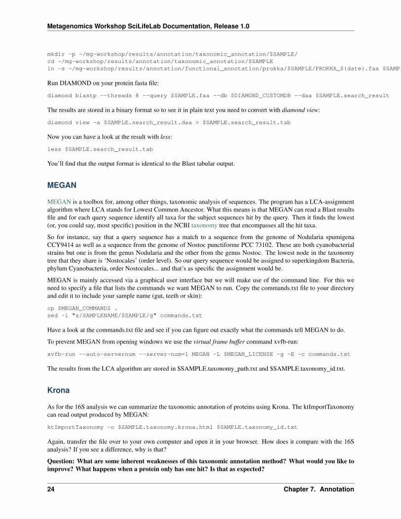
MEGAN

MEGAN is a toolbox for, among other things, taxonomic analysis of sequences. The program has a LCA-assignmentalgorithm where LCA stands for Lowest Common Ancestor. What this means is that MEGAN can read a Blast resultsfile and for each query sequence identify all taxa for the subject sequences hit by the query. Then it finds the lowest(or, you could say, most specific) position in the NCBI taxonomy tree that encompasses all the hit taxa.

So for instance, say that a query sequence has a match to a sequence from the genome of Nodularia spumigenaCCY9414 as well as a sequence from the genome of Nostoc punctiforme PCC 73102. These are both cyanobacterialstrains but one is from the genus Nodularia and the other from the genus Nostoc. The lowest node in the taxonomytree that they share is ‘Nostocales’ (order level). So our query sequence would be assigned to superkingdom Bacteria,phylum Cyanobacteria, order Nostocales... and that’s as specific the assignment would be.

MEGAN is mainly accessed via a graphical user interface but we will make use of the command line. For this weneed to specify a file that lists the commands we want MEGAN to run. Copy the commands.txt file to your directoryand edit it to include your sample name (gut, teeth or skin):

cp $MEGAN_COMMANDS .sed -i "s/SAMPLENAME/$SAMPLE/g" commands.txt

Have a look at the commands.txt file and see if you can figure out exactly what the commands tell MEGAN to do.

To prevent MEGAN from opening windows we use the virtual frame buffer command xvfb-run:

xvfb-run --auto-servernum --server-num=1 MEGAN -L $MEGAN_LICENSE -g -E -c commands.txt

The results from the LCA algorithm are stored in $SAMPLE.taxonomy_path.txt and $SAMPLE.taxonomy_id.txt.

Krona

As for the 16S analysis we can summarize the taxonomic annotation of proteins using Krona. The ktImportTaxonomycan read output produced by MEGAN:

ktImportTaxonomy -o $SAMPLE.taxonomy.krona.html $SAMPLE.taxonomy_id.txt

Again, transfer the file over to your own computer and open it in your browser. How does it compare with the 16Sanalysis? If you see a difference, why is that?

Question: What are some inherent weaknesses of this taxonomic annotation method? What would you like toimprove? What happens when a protein only has one hit? Is that as expected?

24 Chapter 7. Annotation

Metagenomics Workshop SciLifeLab Documentation, Release 1.0

Mapping reads and quantifying genes

Overview

So far we have only got the number of genes and annotations in the sample. Because these annotations are predictedfrom assembled reads we have lost the quantitatve information for the annotations. So to actually quantify the genes,we will map the input reads back to the assembly.

There are many different mappers available to map your reads back to the assemblies. Usually they result in a SAMor BAM file. Those are formats that contain the alignment information, where BAM is the binary version of the plaintext SAM format. In this tutorial we will be using bowtie2. You can also take a look at the Bowtie2 documentation.

The SAM/BAM file can afterwards be processed with Picard to remove duplicate reads. Those are likely to be readsthat come from a PCR duplicate.

BEDTools can then be used to retrieve coverage statistics.

Mapping reads with bowtie2

First set up the files needed for mapping. Replace ‘N’ with the kmer you used for the velet assembly:

mkdir -p ~/mg-workshop/results/annotation/mapping/$SAMPLE/cd ~/mg-workshop/results/annotation/mapping/$SAMPLE/ln -s ~/mg-workshop/data/$SAMPLE/reads/1M/${SAMPLE_ID}_1M.1.fastq pair1.fastqln -s ~/mg-workshop/data/$SAMPLE/reads/1M/${SAMPLE_ID}_1M.2.fastq pair2.fastqln -s ~/mg-workshop/results/assembly/$SAMPLE/${SAMPLE}_${kmer}/contigs.fa

Then run the bowtie2-build program on your assembly:

bowtie2-build contigs.fa contigs.fa

Question: What does bowtie2-build do? (Refer to the documentation)

Next we run the actual mapping using bowtie2:

bowtie2 -p 8 -x contigs.fa -1 pair1.fastq -2 pair2.fastq -S $SAMPLE.map.sam

The output SAM file needs to be converted to BAM format and be sorted, either by read name or by leftmost alignmentcoordinate. We’ll sort by coordinate which is the default. For this we will use samtools.:

samtools sort -o $SAMPLE.map.sorted.bam -O bam $SAMPLE.map.sam

Removing duplicates

We will now use MarkDuplicates from the Picard tool kit to identify and remove duplicates in the sorted and indexedBAM file:

java -Xms2g -Xmx32g -jar $PICARD_HOME/MarkDuplicates.jar INPUT=$SAMPLE.map.sorted.bam OUTPUT=$SAMPLE.map.markdup.bam \METRICS_FILE=$SAMPLE.map.markdup.metrics AS=TRUE VALIDATION_STRINGENCY=LENIENT \MAX_FILE_HANDLES_FOR_READ_ENDS_MAP=1000 REMOVE_DUPLICATES=TRUE

Picard’s documentation also exists! Two bioinformatics programs in a row with decent documentation! Take a momentto celebrate, then take a look at it.

Question: Why not just remove all identical pairs instead of mapping them and then removing them?

Question: What is the difference between samtools rmdup and Picard MarkDuplicates?

7.3. Mapping reads and quantifying genes 25

Metagenomics Workshop SciLifeLab Documentation, Release 1.0

Counting mapped reads per gene

We have now mapped reads back to the assembly and have information on how much of the assembly that is coveredby the reads in the sample. We are interested in the coverage of each of the genes annotated in the previous steps bythe PROKKA pipeline. To extract this information from the BAM file we first need to define the regions to calculatecoverage for. This we will do by creating a custom GFF file (actually a GTF file) defining the regions of interest (thePROKKA genes). Here we use an in-house bash script called prokkagff2gtf.sh that searches for the gene regions inthe PROKKA output and then prints them in a suitable format:

prokkagff2gtf.sh ~/mg-workshop/results/annotation/functional_annotation/prokka/$SAMPLE/PROKKA_${date}.gff > $SAMPLE.map.gtf

We then use htseq to count the number of reads mapped to each gene. Here we have to tell htseq that the file is sortedby alignment coordinate -r pos:

htseq-count -r pos -t CDS -f bam $SAMPLE.map.markdup.bam $SAMPLE.map.gtf > $SAMPLE.count

The output file has two columns, the first contains the gene names and the second the number of reads mapped to eachgene. The last 5 lines gives you some summary information from htseq.

Normalizing to Transcripts Per Million (TPM)

So now we have abundance values for genes in the assembly in the form of absolute read counts mapped to each gene.But we have not taken into account that longer genes will get more mapped reads than shorter genes just by beinglonger. Also, if we’d like to compare abundance values between several samples we would have to account for the factthat the total number of reads sequenced (the sequencing depth) may differ significantly between samples.

There are several ways to normalize abundance values in metagenomes. Here we will use the TPM (Transcripts PerMillion) method. For information on TPM and how it relates to other ways to normalize, like RPKM, see this blogpost.

In order to calculate TPM values we need to know:

• The average read length of the sample

• The length of all genes

The average read length can be calculated from the fastq sequence file that you started with, but we’ll save you thetrouble and say it’s ~100 bp.

The gene lengths we can get from the GTF file that you used with htseq:

cut -f4,5,9 $SAMPLE.map.gtf | sed ’s/gene_id //g’ | gawk ’{print $3,$2-$1+1}’ | tr ’ ’ ’\t’ > $SAMPLE.genelengths

Here we extract only the start, stop and gene name fields from the file, then remove the ‘gene_id’ string, print the genename first followed by the length of the gene, change the separator to tab and store the results in the .genelengths file.

Now we can calculate TPM values using the tpm_table.py script:

tpm_table.py -n $SAMPLE -c $SAMPLE.count -i <(echo -e "$SAMPLE\t100") -l $SAMPLE.genelengths > $SAMPLE.tpm

We now have coverage values for all genes predicted and annotated by the PROKKA pipeline. Next, we will use theannotations and coverage values to summarize annotations for the sample and produce interactive plots.

Question: Coverage can also be calculated for each contig. Do you expect the coverage to differ for a contig andfor the genes encoded on the contig? When might it be a good idea to calculate the latter?

26 Chapter 7. Annotation

Metagenomics Workshop SciLifeLab Documentation, Release 1.0

Summarize and explore the annotation

Now that we have annotated genes and quantified them in the sample using read mapping we will summarize andexplore the annotations. This we will do by producing interactive plots detailing the proportion of functional categoriessuch as metabolic pathways and orthologous gene families.

KRONA interactive plots

KRONA is a tool that takes as input a table of abundance values and several hierarchical categories and producesHTML files that can be explored interactively. The enzyme annotations from PROKKA are particularly suited for thispurpose because these annotations can be grouped into higher functional categories such as pathways (e.g. glycolysis)and pathway classes (e.g. energy metabolism) for enzymes. Similarly, COG annotations can be summed up into highercategories such as “Carbohydrate transport and metabolism” and “Metabolism”.

First we will create a new directory for the krona output and link to the necessary files:

mkdir -p ~/mg-workshop/results/annotation/functional_annotation/krona/$SAMPLEcd ~/mg-workshop/results/annotation/functional_annotation/krona/$SAMPLE/ln -s ~/mg-workshop/results/annotation/mapping/$SAMPLE/$SAMPLE.tpmln -s ~/mg-workshop/results/annotation/functional_annotation/prokka/$SAMPLE/PROKKA.$SAMPLE.ecln -s ~/mg-workshop/results/annotation/functional_annotation/prokka/$SAMPLE/PROKKA.$SAMPLE.cogln -s ~/mg-workshop/results/annotation/functional_annotation/minpath/$SAMPLE/PROKKA.$SAMPLE.kegg.minpathln -s ~/mg-workshop/results/annotation/functional_annotation/minpath/$SAMPLE/PROKKA.$SAMPLE.metacyc.minpath

Next, use the in-house genes.to.kronaTable.py script to produce the tabular output needed for KRONA.

For Metacyc pathways (from enzymes, only considering pathways predicted by MinPath):

genes.to.kronaTable.py -i PROKKA.$SAMPLE.ec -m ~/mg-workshop/reference_db/metacyc/ec.to.pwy -H ~/mg-workshop/reference_db/metacyc/pwy.hierarchy -n $SAMPLE -l <(grep "minpath 1" PROKKA.$SAMPLE.metacyc.minpath) -c $SAMPLE.tpm -o $SAMPLE.krona.metacyc.minpath.tab

For KEGG pathways (from enzymes, only considering pathways predicted by MinPath):

genes.to.kronaTable.py -i PROKKA.$SAMPLE.ec -m ~/mg-workshop/reference_db/kegg/ec.to.pwy -H ~/mg-workshop/reference_db/kegg/pwy.hierarchy -n $SAMPLE -l <(grep "minpath 1" PROKKA.$SAMPLE.kegg.minpath) -c $SAMPLE.tpm -o $SAMPLE.krona.kegg.minpath.tab

For COG annotations:

genes.to.kronaTable.py -i PROKKA.$SAMPLE.cog -m ~/mg-workshop/reference_db/cog/cog.to.cat -H ~/mg-workshop/reference_db/cog/cat.hierarchy -n $SAMPLE -c $SAMPLE.tpm -o $SAMPLE.krona.COG.tab

Finally, use Kronatools ktImportText script to generate the HTML files:

ktImportText -o $SAMPLE.krona.metacyc.minpath.html $SAMPLE.krona.metacyc.minpath.tabktImportText -o $SAMPLE.krona.kegg.minpath.html $SAMPLE.krona.kegg.minpath.tabktImportText -o $SAMPLE.krona.COG.html $SAMPLE.krona.COG.tab

Copy the resulting html files to your local computer with scp as before and open it a browser, like you did for theFastQC output.

Question: What are the main differences between the databases you have worked with: COG, Metacyc andKEGG? Which one do you prefer and why?

Question: What are the main differences between the different samples (gut, skin and teeth)? Compare withresults from other groups. Can you, for instance, find differences in degradation of compounds?

Enjoy!

7.4. Summarize and explore the annotation 27