
Meta-Analysis in Economics - Purdue University · Meta-regression (fixed, random and mixed models),...
103
Meta-Analysis in Economics An Introduction Raymond J.G.M. Florax Henri L.F. de Groot
Transcript of Meta-Analysis in Economics - Purdue University · Meta-regression (fixed, random and mixed models),...

Meta-Analysis in Economics
An Introduction
Raymond J.G.M. Florax
Henri L.F. de Groot

© Florax/de Groot 20092
Our coordinates
Raymond J.G.M. Florax
Dept. of Agricultural Economics – Purdue University
E-mail: [email protected]
Henri L.F. de Groot
Dept. of Spatial Economics – VU University Amsterdam
E-mail: [email protected]
© Florax/de Groot 20093
Overview of topics
1. What is meta-analyis?
Basics, ‗what‘ and ‗why‘, caveats
2. Applicability in economics
Some examples, selection of topic, getting started
3. Combining research results
Vote-counting, combining p-values, heterogeneity and dependence, fixed and random effects methods
4. Meta-regression analysis
Meta-regression (fixed, random and mixed models), panel data
structure, publication bias, heterogeneity, and dependence

What is meta-analysis?
© Florax/de Groot, 20094

© Florax/de Groot 20095
A history of economic research
Exponential growth of studies/knowledge
Use of English as the ―lingua franca‖
Competition of ideas
Quantitative analysis vs. narrative reviews of empirical research
Growth of (computer-intensive) simulation and calibration with
concurrent need for ―stylized facts‖
Policy makers increasingly ask for quantitative information to
underpin policy initiatives

© Florax/de Groot 20096
Why meta-analysis?
―Flood of numbers‖ (Heckman, 2001)
Take stock of knowledge and accumulate instead of duplicate (―lack of collective memory‖)
Conflicting evidence requires methodology of plausible inference (Goldfarb, 1995)
Applied researchers and policy makers need to make sense of ‗hotch potch‘ of research findings
Application of value transfer
Can yield ‗new‘ insights
© Florax/de Groot 20097
What is meta-analysis?
Meta-analysis refers to the statistical analysis of a large
collection of results from individual studies for the purpose of
integrating the findings. It connotes a rigorous alternative to the
causal, narrative discussions of research studies which typify our
attempt to make send of the rapidly expanding research literature.
Glass (1976)

© Florax/de Groot 20098
Pivotal elements of the definition
Statistical: toolbox
Rigorous or ‗objective‘ or ‗systematic‘
Integration of large collection of studies
Alternative for narrative reviews … or complement

© Florax/de Groot 20099
History of meta-analysis
Strong tradition in medicine and psychology
Natural to apply in experimental sciences
Increase sample size by combining experiments
―Tool to save lives‖

Applicability in economics
© Florax/de Groot, 200910

© Florax/de Groot 200911
Meta-analysis in economics
Relatively recent (since early 1980s)
Started in environmental economics
More recently used in labor economics, industrial organization,
marketing, macroeconomics
Characteristics and trends of meta-analysis in economics
(from Florax and Poot, Sønderborg, 2007)

© Florax/de Groot, 200912
The average annual growth rate has been about 22%
Exponential growth
0
5
10
15
20
25
30
35
40
45
50
1975 1980 1985 1990 1995 2000 2005 2010
year
nu
mb
er
of
pa
pe
rs

© Florax/de Groot, 200913
Some general observations
In economics, between 1980 and 2006, 300 papers, of which 1/6
are introductions to meta-analysis or theoretical contributions
T.D. Stanley (2001) J. of Economic Perspectives most cited intro
to meta-analysis in economics (1 Aug 2007: 128 Google scholar
citations, GSC)
About 80% of published meta-analysis applications in economics
use Meta-Regression Analysis (MRA, including ANOVA)
About 25% of published applications to date test/correct for
publication bias; however, the percentage is increasing over time

© Florax/de Groot, 200914
Citations
Within business and economics broadly, meta-analysis remains
more cited in marketing and finance than in economics
Most cited (515 GSC) is Sheppard et al. (1988) in J. of Consumer
Research, on the theory on reasoned action
In mainstream economics, 15 meta-analyses have more than or
close to 100 GSC
The average number of GSC is 38.5 (with s.d. 56.8)

© Florax/de Groot, 200915
“Mainstream economics” (n = 125)
Published in economics journals
Primary data from non-experimental research
No pooling of primary data
Authors are economists
Article is in English
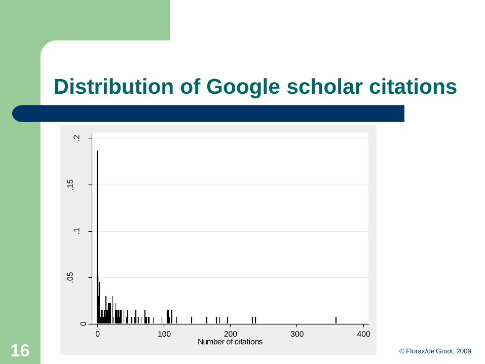
© Florax/de Groot, 200916
Distribution of Google scholar citations 0
.05
.1.1
5.2
Density
0 100 200 300 400Number of citations

© Florax/de Groot, 200917
Distribution across fields
Macroeconomics and Monetary Economics 5.9
International Economics 6.4
Financial Economics 2.0
Public Economics 11.4
Health, Education and Welfare 11.9
Labor and Demographic Economics 8.9
Industrial Organization 4.5
Business Administration and Business Economics, Marketing, Accounting 8.9
Economic Development, Technological Change and Growth 8.4
Agricultural and Natural Resource Economics; Environmental and Ecological Economics 21.8
Urban, Rural and Regional Economics 9.9
100.0

© Florax/de Groot, 200918
0
.005
.01
.015
.02
Density
0 100 200 300Number of research documents used
Number of research documents used

© Florax/de Groot, 200919
Number of effect sizes0
.001
.002
.003
.004
Den
sity
0 500 1000 1500Size of meta-sample

© Florax/de Groot, 200920
Only 15% of meta-analyses use one effect size per study approach
Number of effect sizes per document0
.1.2
.3.4
Den
sity
0 20 40 60effperdoc
© Florax/de Groot, 200921
Common effect sizes
Regression coefficients with a common metric
Elasticities
Family of t and related statistics (r, z)
Categorical levels for ordered probit analysis
Other effect sizes are relatively less commonly used – choices are
more conservative than in other social sciences
© Florax/de Groot, 200922
Summarizing effect sizes
MRA is the most common approach
OLS is increasingly replaced by WLS
Vote counting (frequency cross tabulation) remains common as a
precursor to contingency table analysis and discrete choice
models
Not yet widely applied in economics:
– Non-parametric methods (such as rough set analysis)
– Hierarchical multi-level models
– Bayesian approaches

© Florax/de Groot, 200923
How to do a meta-analysis?
Selection of topic
Construct representative sample of studies
Construct a database
Perform the statistical analysis
– Description of effect sizes
– Exploratory analysis (e.g., with visual tools)
– Analysis of variance
– Test for heterogeneity and dependence
– Meta-regression

© Florax/de Groot, 200924
Selection of a topic
Research results (‗effect sizes‘) in quantitative format…
… and comparable
Sufficient number of studies
© Florax/de Groot, 200925
Construct representative sample
Develop a strategy
Use of search engines, snow-balling, etc.
Published versus unpublished studies
Balanced samples over time and/or space
Deal with the ―file drawer‖

© Florax/de Groot, 200926
Sampling processes – I
Double sampling process
First, literature retrieval and second, measurement sampling
Literature retrieval
- state-of-the-art-reviews
- search engines
- deal with potential selection effects (published vs.
unpublished, language, location, time-period, etc.)
Relevant questions:
- do you need as many studies as possible?
- can you select on quality or other criteria?
- what is unpublished?
- can you open the ‗file drawer‘?

© Florax/de Groot, 200927
Sampling processes – II
Selection of measurements from studies
One vs. all measurements
One overall measurement (average)
- lacking precision estimate
- arbitrary and loss of information
All measurements
- outliers and ―perverse‖ results
- precision
- does this always make sense (e.g., hetero-correction)
Document both sampling processes carefully

© Florax/de Groot, 200928
Building a database – I
Look at other databases
Make a design, and document info:
- reference
- effect size (definition and associated standard error)
- estimation characteristics, etc.
Start with alphanumerical information
Make ONE database, with automatic links, make graphs

© Florax/de Groot, 200929
Building a database - II
Two examples:
- Dalhuisen et al. (2001): demand elasticities for residential
water demand
- Mulatu et al. (2002): competitiveness and environmental
stringency
Available at http://web.ics.purdue.edu/~rflorax/data.htm
Proper management is essential (colors, fonts, comments, etc.)
Make sure your database can be published online (personal
website or through a journal)
© Florax/de Groot, 200930
Construct database – I
Think of ‗moderators‘
Develop a protocol for coding
Careful coding is required: huge investment
Keep track of your decisions (take notes)
You have to face ‗bad reporting‘
Keep database up to data

© Florax/de Groot, 200931
Construct database – II
Typical database contains:
Publication details
Estimate of effect size (and associated standard error)
Estimation characteristics (functional form, # of observations,
control variables, etc.)
Moderator variables (type of data, geographical location, time-
period, etc.)
© Florax/de Groot, 200932
Statistical analysis
Description of effect sizes (histograms, etc.)
Analysis of variance (differences in (conditional) means, etc.)
Vote counting
Combining effect sizes (fixed and random effects)
Meta-regression (fixed and mixed effects)

© Florax/de Groot, 200933
Problems in meta-analysis
Publication bias (and other selection effects, e.g., language)
Comparability of effect sizes
Heterogeneity among studies (e.g., quality differences)
Dependence of data
© Florax/de Groot, 200934
Publication bias
Tendency to publish ―positive‖ results
– Confirming common sense
– Focus on statistical significance
Studies ending up in the ‗file drawer‘
Underlines importance of sample selection
There are techniques to detect publication bias!

© Florax/de Groot, 200935
Comparability of effect sizes
‗Making‘ estimates comparable — measure in common, uniform
metric (e.g., elasticity)
But, is an elasticity taken from a double-log specification
comparable to a segment elasticity?
Long-run versus short-run elasticity?
Lack of experimental setting in economics!
How much of a purist should one be?

© Florax/de Groot, 200936
Heterogeneity
Again, lack of experimental setting and culture of replication in
economics
Obvious sources of heterogeneity are differences over space,
time, etc.
Several sources of heterogeneity are, however, difficult to identify
and measure
Methods to detect and account for heterogeneity
© Florax/de Groot, 200937
Dependence
Problem of taking multiple estimates from same study
But also problem of taking estimates from studies that use the
same data, the same specification, etc.
Problem comparable to autocorrelation in time-series
econometrics

© Florax/de Groot, 200938
Practice of doing meta-analysis
Meta-analysis and value transfer
Alternatives to meta-analysis
Prospects and significance of meta-analysis

© Florax/de Groot, 200939
Value transfer – I
Transfer of results for (a) studied site(s) to unstudied sites
Synonymous to ―benefit transfer‖
Similar to ‗forecasting‘ in time series econometrics
Advantages
- cost effective
- improved use of information
Used in policymaking
- USA: EPA (value of life), NOAA (spills)
- UK: landfill tax

© Florax/de Groot, 200940
Value transfer – II
Different types of value transfer:
- (mean) value
- demand or bid function (―function transfer‖)
- value or function based on meta-analysis
Accuracy of results is (still) disappointing
- just transferring values is naïve
- use of meta-analysis may be important
- role of preferences and personal characteristics
- problem: dependence on research design

© Florax/de Groot, 200941
Why are there sceptics in economics?
―Nonlinear interactive dynamics in research priorities‖
(e.g., Brock and Durlauf, 1999)
Quality of research is multi-dimensional and accounting for quality
variation subjective
Statistical foundations from experimental sciences do not fit
―Competition of ideas‖, no ―encompassing theory‖ and/or no
―natural constants‖
Replication would be helpful, but is not practiced

© Florax/de Groot, 200942
Alternatives to meta-analysis – I
Meta-analysis is ―irrelevant‖ and ―misses the point‖ (Rubin)
interpolation: summing up imperfect studies
versus
extrapolation: project findings of an ideal study
Response surface of the ideal study
3D landscape projection of size, time, place, treatment, etc.

© Florax/de Groot, 200943
Alternatives to meta-analysis – II
Consider only the ―best‖ study or the largest study
Slavin (1986, 1995): ―best evidence synthesis‖
- combine series of ―best studies‖
How do we define ―best‖?

© Florax/de Groot, 200944
Relevance of meta-analysis
Complement to ‗traditional‘ literature reviews
Increased accuracy
Allows non-testable hypotheses to be tested
But, causal inferences are impossible (correlation)!
Develop methods relevant for economics
Link meta-analysis to theory
Explore behavioral basis and context

© Florax/de Groot, 200945
Conclusion
Useful methodology
Needs theoretical underpinning (no empiricism)
Reasonably objective (at least transparent)
Several applications in applied and policy-oriented research
Time-consuming construction of database
Several problems and pitfalls, but in many cases surmountable
May provide guidance for future theory development and empirics

Combining research results
© Florax/de Groot, 200946

© Florax/de Groot, 200947
Vote counting – I
Counting positive, negative and zero results
Implicit in literature reviews
Flawed: Type-II errors do not cancel
Wrong inference when # studies increases
Low power for medium to small effect sizes

© Florax/de Groot, 200948
Vote counting – II
Drawbacks
- ignores sample size
- nose-length victory or walk-over
Not always relevant in economics (values: WTP)
Cross tabulate with moderators
Example: competitiveness data

© Florax/de Groot, 200949
Combining probability values
Only for one-sided p-values direction of the effect
H0: qi = 0, for i = 1, …, k
H1: qi 0, for at least one i, or
H1: qi 0, for i = 1, …, k, with qj 0, for at least one j
Asymmetrical information content
© Florax/de Groot, 200950
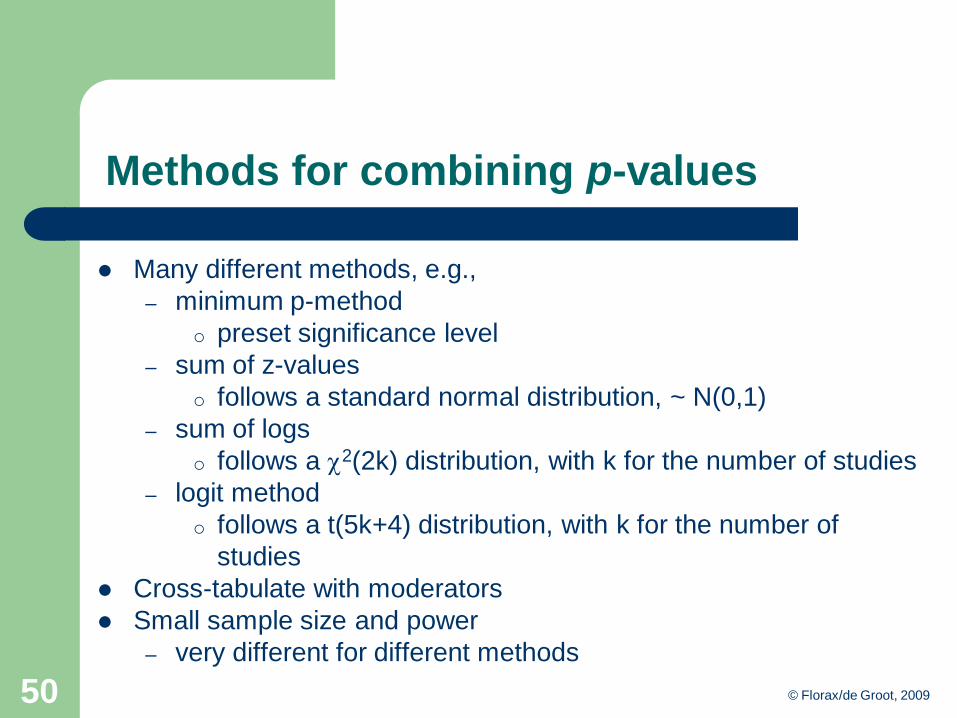
Methods for combining p-values
Many different methods, e.g.,
– minimum p-method
o preset significance level
– sum of z-values
o follows a standard normal distribution, ~ N(0,1)
– sum of logs
o follows a c2(2k) distribution, with k for the number of studies
– logit method
o follows a t(5k+4) distribution, with k for the number of
studies
Cross-tabulate with moderators
Small sample size and power
– very different for different methods
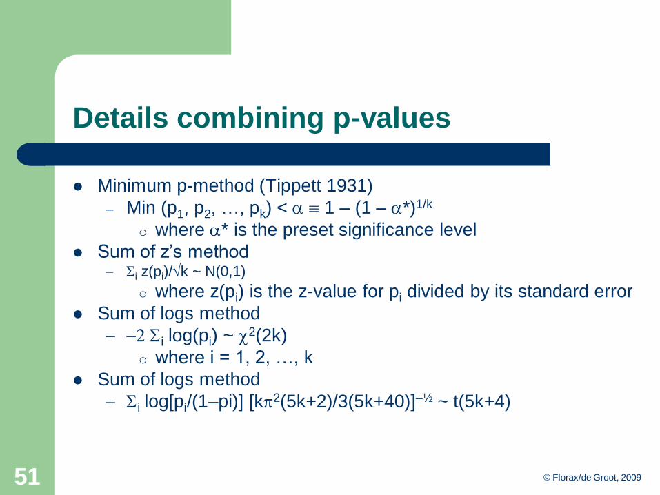
Details combining p-values
Minimum p-method (Tippett 1931)
– Min (p1, p2, …, pk) < a 1 – (1 – a*)1/k
o where a* is the preset significance level
Sum of z‘s method- Si z(pi)/k ~ N(0,1)
o where z(pi) is the z-value for pi divided by its standard error
Sum of logs method
- -2 Si log(pi) ~ c2(2k)
o where i = 1, 2, …, k
Sum of logs method
- Si log[pi/(1–pi)] [kp2(5k+2)/3(5k+40)]–½ ~ t(5k+4)
© Florax/de Groot, 200951

Example competitiveness
Taken from Mulatu et al. (2003)
© Florax/de Groot, 200952
COMBINED SIGNIFICANCE LEVELS ACCORDING TO STUDY TYPE
Min of p-level, one-sided Count of Type study
Type study Total Type study Total Type study Minimum p critical level H0
Econometric 0.000001 Econometric 655 Econometric 0.000001 0.000078 rejected
Leontief 0.000003 Leontief 19 Leontief 0.000003 0.002696 rejected
Exploratory 0.006086 Exploratory 55 Exploratory 0.006086 0.000932
All studies 0.000001 All studies 729 All studies 0.000001 0.000070 rejected
Sum of z-value of p-level Count of Type study
Type study Total Type study Total Type study Sum of z prob H0
Econometric -336.098 Econometric 655 Econometric -13.132 0.000 rejected
Leontief -35.057 Leontief 19 Leontief -8.043 0.000 rejected
Exploratory -18.349 Exploratory 55 Exploratory -2.474 0.007 rejected
All studies -389.504 All studies 729 All studies -14.426 0.000 rejected
Sum of log of p-level Count of Type study
Type study Total Type study Total Type study Sum of logs prob H0
Econometric ####### Econometric 655 Econometric 2695.647 0.000 rejected
Leontief -89.482 Leontief 19 Leontief 178.964 0.000 rejected
Exploratory -69.815 Exploratory 55 Exploratory 139.631 0.030 rejected
All studies ####### All studies 729 All studies 3014.242 0.000 rejected
Sum of logit of p-level Count of Type study
Type study Total Type study Total Type study Logit prob H0
Econometric -740.981 Econometric 655 Econometric 16.055 0.000 rejected
Leontief -84.901 Leontief 19 Leontief 12.669 0.000 rejected
Exploratory -30.076 Exploratory 55 Exploratory 2.384 0.018 rejected
All studies -855.958 All studies 729 All studies 17.569 0.000 rejected

© Florax/de Groot, 200953
Variation in other effect sizes
Point estimates are always different
Due to:
- sampling
- population effect size is the same (homogeneity)
- use fixed effects model
Due to:
- sampling + “real” differences
- population effect size differs by study (heterogeneity)
- use random effects model
© Florax/de Groot, 200954
Effect sizes – test and exploratory tools
Test for heterogeneity (Q-test)
Visual tools for heterogeneity (forest plot, radial plot)
Example: value of statistical life (VOSL)
- recover VOSL from risk premium included in wages
- see, Miller (2000), Harrison (2002), de Blaeij et al. (2003)
© Florax/de Groot, 200955
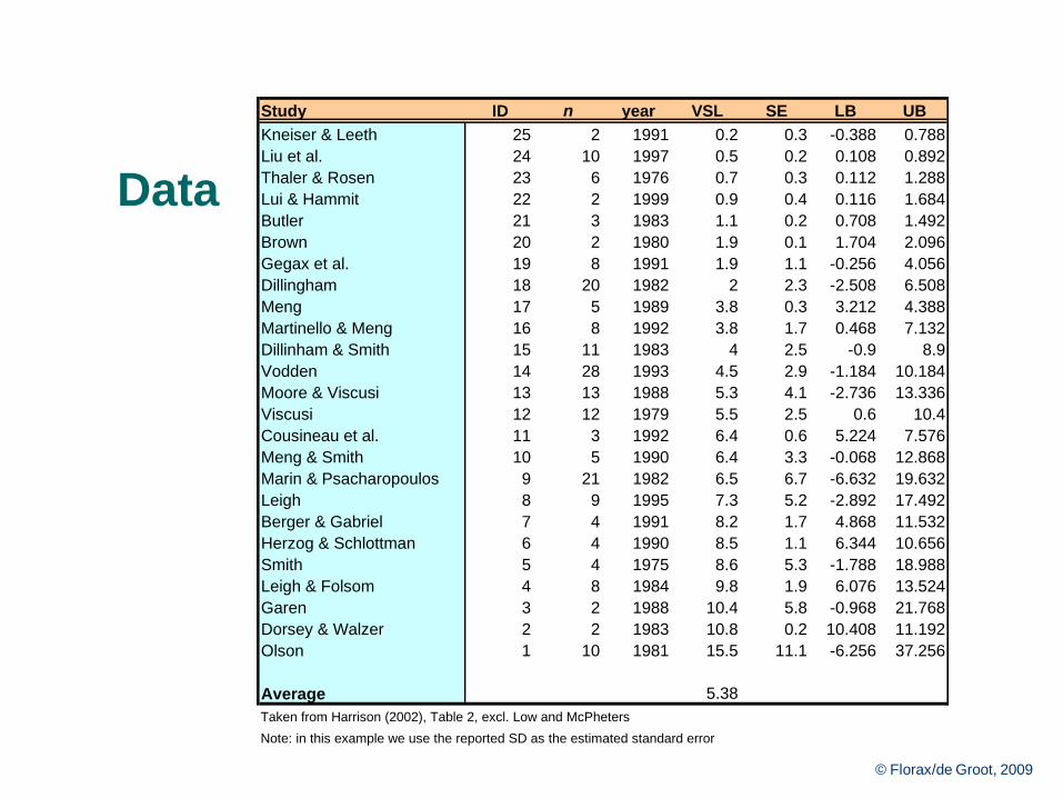
Data
Study ID n year VSL SE LB UB
Kneiser & Leeth 25 2 1991 0.2 0.3 -0.388 0.788
Liu et al. 24 10 1997 0.5 0.2 0.108 0.892
Thaler & Rosen 23 6 1976 0.7 0.3 0.112 1.288
Lui & Hammit 22 2 1999 0.9 0.4 0.116 1.684
Butler 21 3 1983 1.1 0.2 0.708 1.492
Brown 20 2 1980 1.9 0.1 1.704 2.096
Gegax et al. 19 8 1991 1.9 1.1 -0.256 4.056
Dillingham 18 20 1982 2 2.3 -2.508 6.508
Meng 17 5 1989 3.8 0.3 3.212 4.388
Martinello & Meng 16 8 1992 3.8 1.7 0.468 7.132
Dillinham & Smith 15 11 1983 4 2.5 -0.9 8.9
Vodden 14 28 1993 4.5 2.9 -1.184 10.184
Moore & Viscusi 13 13 1988 5.3 4.1 -2.736 13.336
Viscusi 12 12 1979 5.5 2.5 0.6 10.4
Cousineau et al. 11 3 1992 6.4 0.6 5.224 7.576
Meng & Smith 10 5 1990 6.4 3.3 -0.068 12.868
Marin & Psacharopoulos 9 21 1982 6.5 6.7 -6.632 19.632
Leigh 8 9 1995 7.3 5.2 -2.892 17.492
Berger & Gabriel 7 4 1991 8.2 1.7 4.868 11.532
Herzog & Schlottman 6 4 1990 8.5 1.1 6.344 10.656
Smith 5 4 1975 8.6 5.3 -1.788 18.988
Leigh & Folsom 4 8 1984 9.8 1.9 6.076 13.524
Garen 3 2 1988 10.4 5.8 -0.968 21.768
Dorsey & Walzer 2 2 1983 10.8 0.2 10.408 11.192
Olson 1 10 1981 15.5 11.1 -6.256 37.256
Average 5.38
Taken from Harrison (2002), Table 2, excl. Low and McPheters
Note: in this example we use the reported SD as the estimated standard error
© Florax/de Groot, 200956
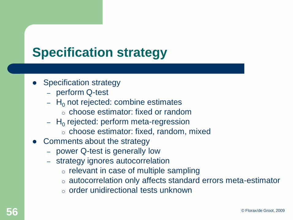
Specification strategy
Specification strategy
– perform Q-test
– H0 not rejected: combine estimates
o choose estimator: fixed or random
– H0 rejected: perform meta-regression
o choose estimator: fixed, random, mixed
Comments about the strategy
– power Q-test is generally low
– strategy ignores autocorrelation
o relevant in case of multiple sampling
o autocorrelation only affects standard errors meta-estimator
o order unidirectional tests unknown

© Florax/de Groot, 200957
Notation and ANOVA – I
Notation
– independent effect sizes for p disjoint groups
– mp effects in each group (p = 1, 2, …, P)
– j-th population effect size in the i-th group is qij
– estimated effect size Tij with conditional variance vij
– variance treated as known for sufficiently large n

Notation and ANOVA – II
Means
– group mean effect Ťi•= Sj wijTij / Sj wij
o where wij = 1/vij
o and vi• = 1 / Sj wij
– grand or overall mean effect Ť••= Sj Sj wijTij / Sj Sj wij
o where v•• = 1 / Sj Sj wij
– test on equality of means based on z-values
o group means normally distributed
o H0: qi• = qo z = (Ťi• – qo) / (vi•)1/2
© Florax/de Groot, 200958

© Florax/de Groot, 200959
Q tests
Between group differences
– H0: q1• = q2• = … = qp•
– QBET = Si wi• (Ťi• – Ť••)2
– follows c2 distribution with p – 1 degrees of freedom
Within group differences
– QW = QW1 + QW2 + … + QWp
– where QWi = Sj wij(Tij – Ťi•)2
– follows c2 distribution with mi – 1 degrees of freedom
Overall differences
– Q = QBET + QW
– Q = Si Sj wij(Tij)2 – (Si Sj wijTij / Si Sj wij)
– follows c2 distribution with k – 1 degrees of freedom

© Florax/de Groot, 200960
Q test considerations
Qualifications
– power is low
– with large sample sizes over-rejection of H0 homogeneity
– potential impact of primary study design flaws
– similarly of publication bias
Computational aspects
– use standard ANOVA
– or standard regression package and WLS regression
– note that WLS estimated standard errors are not correct
o meta-estimator, v•• = 1 / Sj Sj wij
o WLS, v•• = vm / Sj Sj wij
o rescale standard errors with vm
© Florax/de Groot 200961
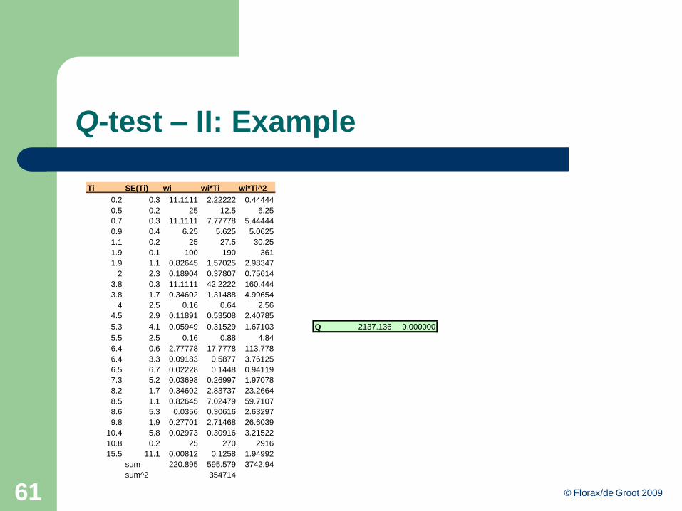
Q-test – II: Example
Ti SE(Ti) wi wi*Ti wi*Ti^2
0.2 0.3 11.1111 2.22222 0.44444
0.5 0.2 25 12.5 6.25
0.7 0.3 11.1111 7.77778 5.44444
0.9 0.4 6.25 5.625 5.0625
1.1 0.2 25 27.5 30.25
1.9 0.1 100 190 361
1.9 1.1 0.82645 1.57025 2.98347
2 2.3 0.18904 0.37807 0.75614
3.8 0.3 11.1111 42.2222 160.444
3.8 1.7 0.34602 1.31488 4.99654
4 2.5 0.16 0.64 2.56
4.5 2.9 0.11891 0.53508 2.40785
5.3 4.1 0.05949 0.31529 1.67103 Q 2137.136 0.000000
5.5 2.5 0.16 0.88 4.84
6.4 0.6 2.77778 17.7778 113.778
6.4 3.3 0.09183 0.5877 3.76125
6.5 6.7 0.02228 0.1448 0.94119
7.3 5.2 0.03698 0.26997 1.97078
8.2 1.7 0.34602 2.83737 23.2664
8.5 1.1 0.82645 7.02479 59.7107
8.6 5.3 0.0356 0.30616 2.63297
9.8 1.9 0.27701 2.71468 26.6039
10.4 5.8 0.02973 0.30916 3.21522
10.8 0.2 25 270 2916
15.5 11.1 0.00812 0.1258 1.94992
sum 220.895 595.579 3742.94
sum^2 354714
© Florax/de Groot 200962
Plot z-scores – I
If variation is random z-scores standard normally distributed
Construct z‘s, make histogram, add standard normal
)1,0(~ Nv
TTz
i
ii
-

© Florax/de Groot 200963
Plot z-scores – II: example
-0.10
0.00
0.10
0.20
0.30
0.40
0.50
-10 -5 0 5 10 15 20 25 30 35 40
z -score
Fra
ctio
n
Ti SE(Ti) wi wi*Ti z-score
0.2 0.3 11.11111 2.222222 -8.320695
0.5 0.2 25 12.5 -10.98104
0.7 0.3 11.11111 7.777778 -6.654028
0.9 0.4 6.25 5.625 -4.490521
1.1 0.2 25 27.5 -7.981042
1.9 0.1 100 190 -7.962084
1.9 1.1 0.826446 1.570248 -0.723826
2 2.3 0.189036 0.378072 -0.302699
3.8 0.3 11.11111 42.22222 3.679305
3.8 1.7 0.346021 1.314879 0.649289
4 2.5 0.16 0.64 0.521517
4.5 2.9 0.118906 0.535077 0.621997
5.3 4.1 0.059488 0.315289 0.635071
5.5 2.5 0.16 0.88 1.121517
6.4 0.6 2.777778 17.77778 6.172986
6.4 3.3 0.091827 0.587695 1.122361
6.5 6.7 0.022277 0.144798 0.56773
7.3 5.2 0.036982 0.26997 0.885345
8.2 1.7 0.346021 2.83737 3.237524
8.5 1.1 0.826446 7.024793 5.276174
8.6 5.3 0.0356 0.306159 1.113923
9.8 1.9 0.277008 2.714681 3.738838
10.4 5.8 0.029727 0.309156 1.32824
10.8 0.2 25 270 40.51896
15.5 11.1 0.008116 0.125801 1.153495
220.895 595.579
Tav 2.696208

© Florax/de Groot 200964
Forest plot – I
-10 -5 0 5 10 15 20 25 30 35 40
VOSL in millions 1996 US$
Stu
dy

© Florax/de Groot 200965
Forest plot – II
Exploratory tool
Presentation tool
- include overall effect
- visualization of for robustness analysis
Note: widest confidence interval should be least influential
(use plotting symbols to signal that)

© Florax/de Groot, 200966
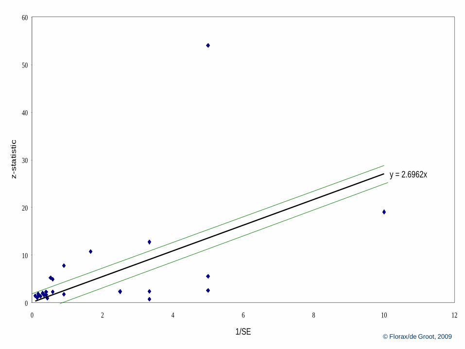
Galbraith diagram – I
Plot z-value (t-value) against reciprocal standard error
Note:
- weight on horizontal axis
- estimated effect size per study (gradient line through origin and
estimate)
- pooled fixed effect (gradient trend line through origin)
- outliers (contribution to Q)
- heteroskedasticity
Use different colors for different type studies

y = 2.6962x
0
10
20
30
40
50
60
0 2 4 6 8 10 12
1/SE
z-s
tatistic
67 © Florax/de Groot, 2009
y = 2.6962x
0
10
20
30
40
50
60
0 2 4 6 8 10 12
1/SE
z-s
tatistic
68 © Florax/de Groot, 2009

y = 2.6962x
0
10
20
30
40
50
60
0 2 4 6 8 10 12
1/SE
z-s
tatistic
y = 10.8 x
69 © Florax/de Groot, 2009
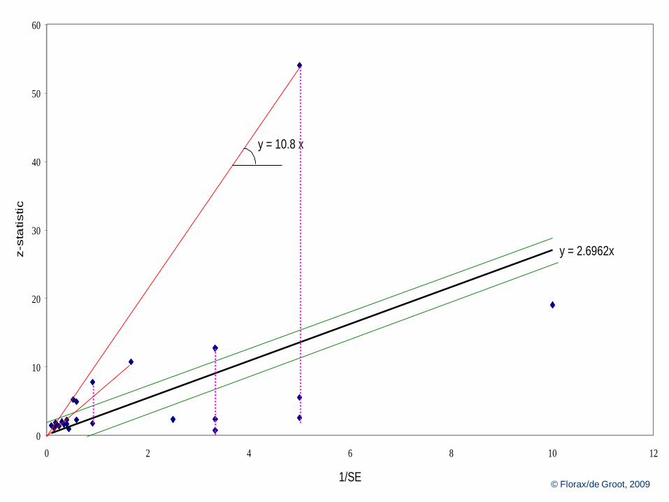
Galbraith diagram – II
y = 2.6962x
0
10
20
30
40
50
60
0 2 4 6 8 10 12
1/SE
z-s
tatistic
y = 10.8 x
70 © Florax/de Groot, 2009

© Florax/de Groot 200971
Combining effect sizes
Fixed effects model
- one identical population effect size
- eventually include observable (known) variation
Random effects model
- population effect sizes differ (drawn from normal distribution)
© Florax/de Groot, 200972
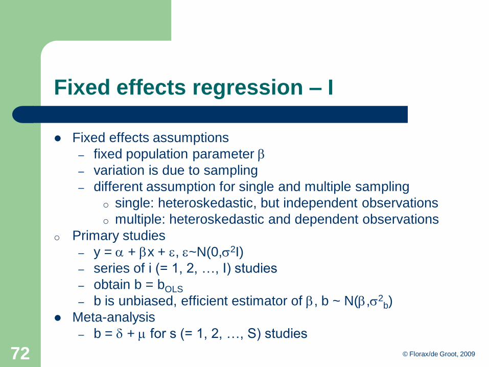
Fixed effects regression – I
Fixed effects assumptions
– fixed population parameter b
– variation is due to sampling
– different assumption for single and multiple sampling
o single: heteroskedastic, but independent observations
o multiple: heteroskedastic and dependent observations
o Primary studies
– y = a + bx + e, e~N(0,s2I)
– series of i (= 1, 2, …, I) studies
– obtain b = bOLS
– b is unbiased, efficient estimator of b, b ~ N(b,s2b)
Meta-analysis
– b = d + m for s (= 1, 2, …, S) studies

© Florax/de Groot, 200973
Fixed effects regression – II
Standard (unweighted) case
– meta-estimator effect size:
– unbiased:
– associated meta-estimator variance:
– quadratic decline variance: increase power
– OLS ignores unequal variance across studies
o each study receives the same weight
S
1iib
S
1d
b
S
1ii
S
1ii )b(E
S
1b
S
1E)d(E
ss
S
1i
2
Sb
2
1b2i2
S
1ii ...
S
1)b(Var
S
1b
S
1Var)d(Var

© Florax/de Groot, 200974
Fixed effects regression – III
Weighted case (use of WLS)
– problem with standard errors
– variance of the fixed effects estimator is:
– variance of the weighted least squares estimator is:
– solution: rescale standard errors with error variance
s
S
1i2
i
1
1)dvar(
s
s
m
S
1i2
i
2
1)dvar(

© Florax/de Groot, 200975
Fixed effects regression – IV
Meta-estimators, naïve
– OLS
o unbiased and consistent
o but inefficient due to homoskedasticity assumption
– White adjusted standard errors
o replace Var(b) = s2(X´X)–1 with s2(X´X)–1(X´WX)(X´X)–1
o estimate W as S = diag[(ei/1–kii)2]
o where kii is the i-th diagonal element of X(X´X)–1X´
o does not exploit knowledge about W
Why naïve?
– no adequate usage of available information about variance
o if information is available
o ad hoc remedy is to use sample size: no asymptotics!

© Florax/de Groot, 200976
Fixed effects regression – V
Meta-estimators, informed
– GLS
o treat conditional variances as known, use WLS
o unbiased and consistent, and more efficient than OLS
o rescale standard errors!
o note: only source heteroskedasticity relates to primary
studies
Implications of multiple sampling
– assumption of independence may be violated
– fixed effects meta-estimator ignoring autocorrelation
o remains unbiased and consistent
o not efficient

Fixed effects regression – VI
Robust meta-estimator
– accounts for heteroskedasticity and autocorrelation
– Huber-White or ―sandwich‖ estimator
– replaces W with an estimate
o accounts for unequal variances
o and nonzero covariances
– implemented through weights
o weights defined by studies
– downside
o does not exploit knowledge about conditional variance
© Florax/de Groot, 200977
© Florax/de Groot, 200978
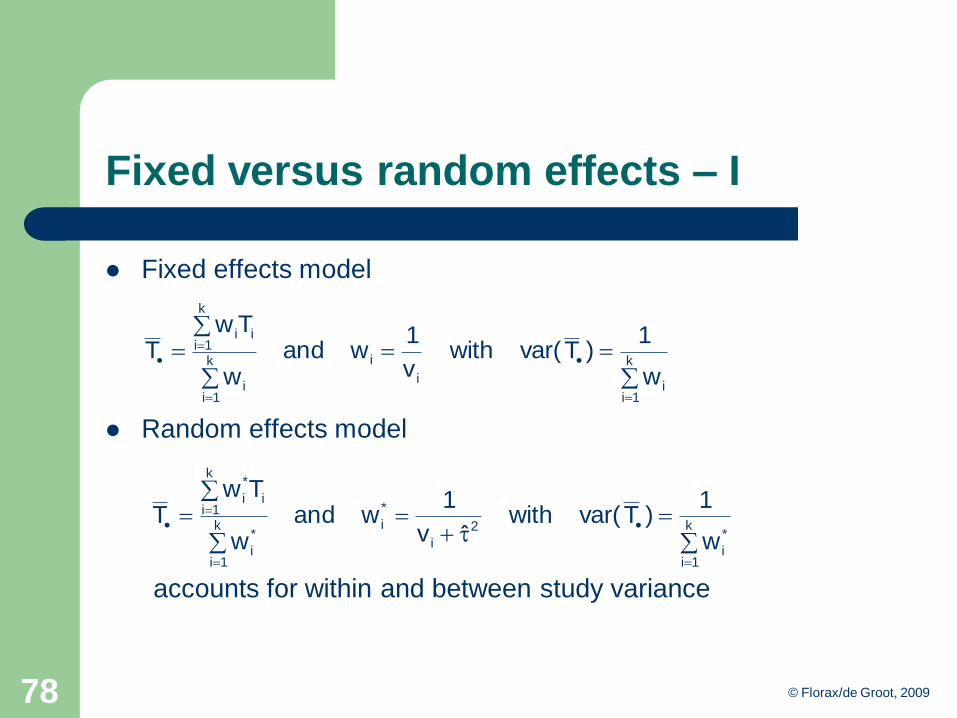
Fixed versus random effects – I
Fixed effects model
Random effects model
accounts for within and between study variance
k
1ii
i
ik
1ii
k
1iii
w
1)Tvar(with
v
1wand
w
TwT
k
1i
*
i
2
i
*
ik
1i
*
i
k
1ii
*
i
w
1)Tvar(with
ˆv
1wand
w
TwT

© Florax/de Groot, 200979
Fixed versus random effects – II
Fixed vs random effects
– regression notation
– fixed effects (FE)
o Ti = qi + ei, qi = b
– random effects (RE)
o Ti = qi + ei, qi = b + mi, where mi ~ N(0,2)
Comparison
– RE more conservative
– RE unrealistic, unjustified distributional assumption
– RE consistent with generalization requirement
– RE more sensitive to publication bias
o greater weight to smaller studies
– crucial point: unexplainable heterogeneity

© Florax/de Groot, 200980
Random effects estimator
How to estimate 2?
– weighted non-iterative method of moments
also known as DerSimonian-Laird estimator
preferable to the unweighted version
– maximum likelihood
involves assuming Ti~N(qi,si2) and qi~N(m,2)
requires nonlinear optimization
ML or REML, accounting for m and 2 based on the same
data
– alternative based on empirical Bayes
– use of REML most appropriate
see Thompson and Sharp (1999)
© Florax/de Groot, 200981
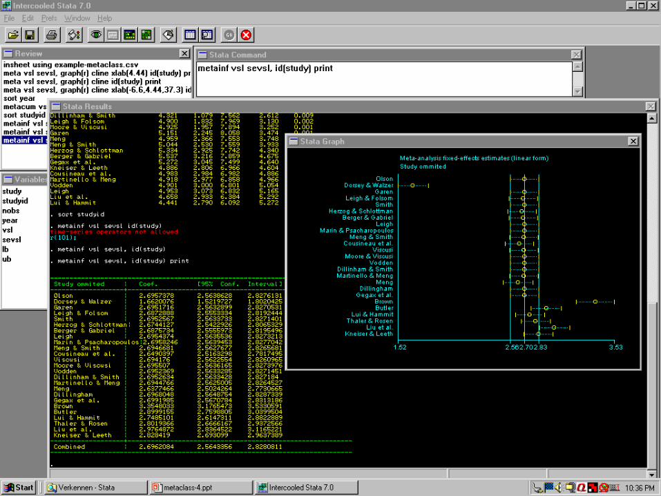
Example: VOSL using StataTM
Example
– Value Of Statistical Life (VOSL)
– dataset provided on website class
User-defined Stata routines
– meta (fixed and random overall effect, forest plot)
– metacum (cumulative meta-analysis over time, plus graph)
– metainf (influence of individual studies, plus graph)


© Florax/de Groot, 200985
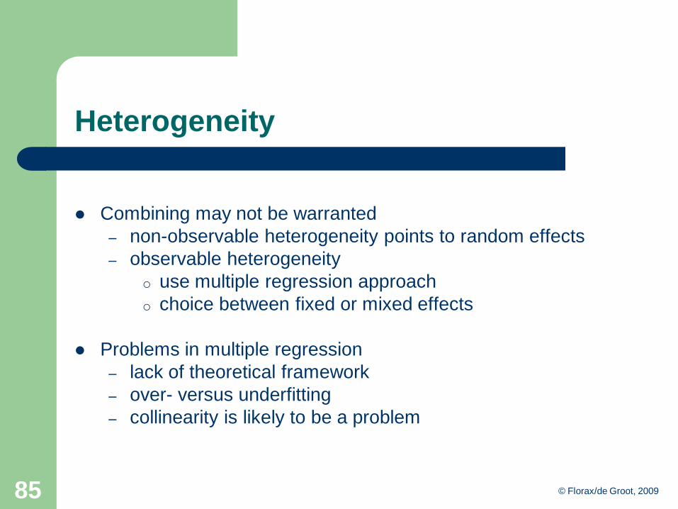
Heterogeneity
Combining may not be warranted
– non-observable heterogeneity points to random effects
– observable heterogeneity
o use multiple regression approach
o choice between fixed or mixed effects
Problems in multiple regression
– lack of theoretical framework
– over- versus underfitting
– collinearity is likely to be a problem

© Florax/de Groot, 200986
Fixed and random effects models
Meaning different from standard econometrics!
Estimation too!
Ongoing debate!
- distributional assumptions
- generalization
- sensitivity to publication bias
- unobservable heterogeneity
Mixed effects models more general

Meta-regression analysis
© Florax/de Groot, 200987
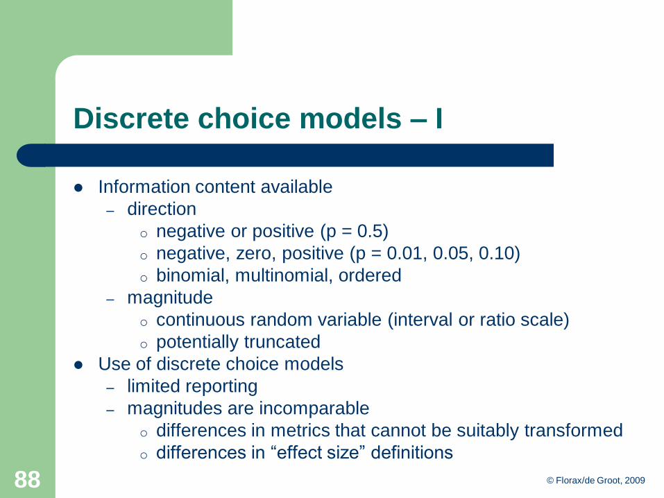
Discrete choice models – I
Information content available
– direction
o negative or positive (p = 0.5)
o negative, zero, positive (p = 0.01, 0.05, 0.10)
o binomial, multinomial, ordered
– magnitude
o continuous random variable (interval or ratio scale)
o potentially truncated
Use of discrete choice models
– limited reporting
– magnitudes are incomparable
o differences in metrics that cannot be suitably transformed
o differences in ―effect size‖ definitions
© Florax/de Groot, 200988

Discrete choice models – II
Analysis of p-values
– categorize p-values in discrete classes
– multinomial or ordered logit/probit
– loss of information content
o caused by transformation
o interpretation different (cumbersome for continuous)
Relation between continuous and discrete choice model
– avoid restricted [0,1] domain
o transform p-values to z –values
– calculate estimated average z-values for moderators
o add coefficient of the constant
– transform average z-values to marginal effects
o assuming a normal distribution is appropriate
© Florax/de Groot, 200989

Example ordered probit
Mulatu et al. (2003)– heterogeneity of effect size measures
– interest in direction of effecto stringency environmental regulation
o competitiveness, measured with trade flows
– ordered probit model
© Florax/de Groot, 200990

Ordered probit
© Florax/de Groot, 200991
Table 4. Results for an ordered probit specification of four different versions Variable
a
FULL MODEL RESTRICTED MODEL FULL MODEL WITH
HETEROSCEDASTICITY
CORRECTION
RESTRICTED MODEL WITH
HETEROSCEDASTICITY
CORRECTION
Parameter t-ratio Parameter t-ratio Parameter t-ratio Parameter t-ratio
Constant -93.3521** -2.4944 -83.0836** -2.2193 -144.5900 -1.3025 -136.7290 -1.2751
EXPLOR -2.8184** -2.2931 -2.3402** -2.3849 -4.0632* -1.8693 -3.5869** -2.1038
LEONTIEF -4.0493** -2.3801 -3.8307** -2.9387 -5.6452** -2.2499 -5.2541** -2.6499
ECTRBETA 1.1876 0.6083 0.9051 0.5920 1.3686 0.5964 1.2818 0.6515
ECTRELAS 1.0634 0.5422 0.7652 0.5030 1.1414 0.4922 1.0433 0.5438
POLLINT -0.4930* -1.6912 -0.4603 -1.6022 -0.6546 -1.1147 -0.6283 -1.1302
NONRESB 0.0015** 0.0070 -0.0272 -0.1312 -0.0849 -0.2256 -0.1074 -0.2953
TSPANY -0.2399 -0.3174 -0.1836 -0.2373
YEAR 52.5105** 2.8018 47.0308** 2.5005 80.1253 1.4097 75.8014 1.3828
YLEVEL -0.5515 -0.8245 -0.5729 -0.7116
YBALANCE 0.0694 0.1705 0.0673 0.1341
STRQUAL -2.6706** -2.6138 -2.9242** -3.9038 -4.3770** -2.6975 -4.5953** -3.2076
STRINDEX -5.2495** -4.4644 -5.3717** -5.5432 -7.5153** -3.7422 -7.7041** -4.1216
INDDATA -4.7557** -4.1439 -4.7392** -4.9177 -6.5054** -3.9287 -6.4530** -4.4047
CROSSSEC -1.9889* -1.8757 -1.6263** -4.3663 -2.2795** -2.0726 -2.0322** -4.8563
PANEL -4.2817** -6.8627 -4.5060** -8.4377 -5.4247** -4.6298 -5.4564** -4.9443
ESTOLS -2.3848** -4.7578 -2.6427** -7.6198 -3.1607** -3.0639 -3.2196** -3.5475
ESTHET -0.2293 -0.6868 -0.0087 -0.0192
HOMOD -1.9558** -2.3245 -1.4208** -1.9785 -2.7653** -2.1653 -2.2254** -2.0557
LDCRATOR 1.8289** 9.4745 1.9088** 10.1022 2.8211** 3.9452 2.9153** 4.1201
TFBILAT -1.2413* -1.7184 -1.2528* -1.8359 -1.1237 -1.3556 -1.0457 -1.4279
Mu(1) 4.3028 16.3746 4.2633 16.9923 5.5797 5.5141 5.5567** 6.0855
NOBS 0.2615 2.6047 0.2630 2.7520
Log-L -235.321 -236.599 -220.146 -220.773
Log-L(0) -386.529 -386.529 -386.529 -386.529 aThe dependent variable is coded with 0 for negative effect sizes, 1 for effect sizes that are not significantly
different from zero, and 2 for positive effect sizes
* = significant at 10 % level of significance.
** = significant at 5% level of significance.

© Florax/de Groot, 200992
Meta-regression: fixed effects – I
Fixed effects assumptions
– fixed population parameters b, (k×1) vector
– variation is due to sampling
– different assumption for single and multiple sampling
o single: heteroskedastic, but independent observations
o multiple: heteroskedastic and dependent observations
Primary studies
– y = a + bx + e, e~N(0,s2I)
– heterogeneous series of i (= 1, 2, …, I) studies
– obtain b = bOLS
– b is unbiased, efficient estimator of b, b ~ N(b,s2b)

© Florax/de Groot, 200993
Meta-regression: fixed effects – II
Meta-analysis
– b = d + Xg + m for s (= 1, 2, …, S) studies
Different estimators
– OLS: not efficient
– OLS with White or Huber-White adjustments
discards knowledge of conditional variance
– fixed effects, WLS with transformation
more efficient than OLS
heteroskedasticity only related to conditional variance
– weighted with White or Huber-White adjustments, no
transformation
incorporates knowledge about conditional variance …
as well as other x-related heteroskedasticity
© Florax/de Groot, 200994
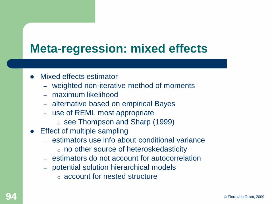
Meta-regression: mixed effects
Mixed effects estimator
– weighted non-iterative method of moments
– maximum likelihood
– alternative based on empirical Bayes
– use of REML most appropriate
o see Thompson and Sharp (1999)
Effect of multiple sampling
– estimators use info about conditional variance
o no other source of heteroskedasticity
– estimators do not account for autocorrelation
– potential solution hierarchical models
o account for nested structure

Specification of moderator variables
– lack of theory, but not completely
o demand elasticities: income
o risk change: initial level
o relation between different definitions consumer surplus
– avoid excessive use of dummy variables
o sensible grouping of study design characteristics
– differences in specification primary studies
o particularly different conditioning variables
o under vs. overspecification of primary models
Check for multicollinearity
– problems with standard errors
– condition number
© Florax/de Groot, 200995
Multicollinearity

© Florax/de Groot, 200996
Misspecification
Primary study misspecification
– heteroskedasticity
o meta-estimator b remains unbiased
o influence on weights in fixed and mixed models
– autocorrelation
o effects similar to heteroskedasticity
– omitted variable bias
o potentially carries over to meta-estimator b
Meta-regression misspecification
– check as you would do with primary study
– select appropriate estimator

Single versus multiple sampling
– heteroskedasticity inherent in both cases
– autocorrelation likely a problem in case of multiple sampling
Reasons for single sampling preference
– even if multiple measurements are available
o avoid negative impact of autocorrelation
o reduces impact of publication bias
o only preferred estimate is ―correct‖
Reasons for multiple sampling
– uses more information
o potentially less bias and inefficiency
– avoids use of selection criterion
o note: implicitly author‘s selection criterion is used
© Florax/de Groot, 200997
Sampling and implications

Multi-level methods – I
Dealing with multiple sampling
– use appropriate estimator accounting for
o heteroskedasticity (conditional variance)
o within-study autocorrelation
– account for structure of the data
o nested structure
o two error terms
o study and measurement level
© Florax/de Groot, 200998
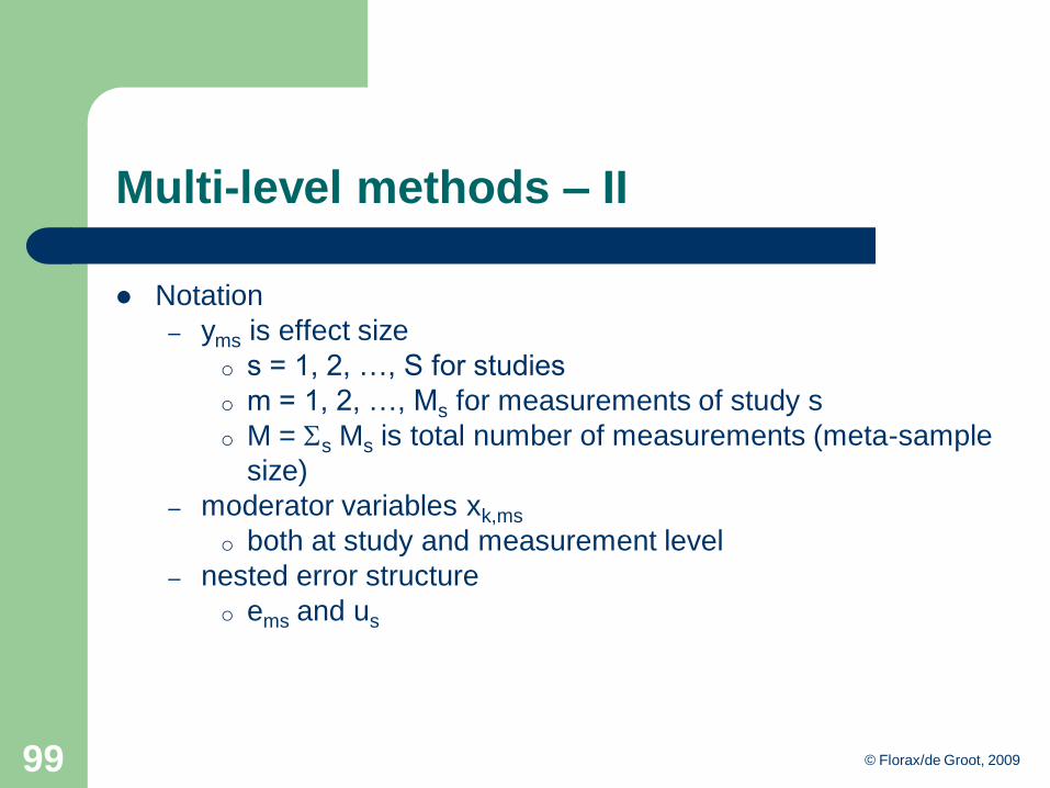
Multi-level methods – II
Notation
– yms is effect size
o s = 1, 2, …, S for studies
o m = 1, 2, …, Ms for measurements of study s
o M = Ss Ms is total number of measurements (meta-sample
size)
– moderator variables xk,ms
o both at study and measurement level
– nested error structure
o ems and us
© Florax/de Groot, 200999

Multi-level methods – III
Specification
– yms = b0 + Sk bkxk,ms + ems + us
– ems~N(0,s2e) and us~N(0,s2
u)
– multi-level model, hierarchy in error structure
Estimator
– b = (b0, b1, …, bk)´ and b = (X´T–1X)–1X´T–1y
o where T = WSW
o W is diagonal matrix with weights
o S is block-diagonal error variance-covariance matrix
– s2 = (s2e, s
2u) and s2 = (Z´(T*)–1Z)–1Z´(T*)–1vec(y*)
o where Z is M22 design matrix with 1 if S contains s2e or s2
u
o y* cross-product matrix of residuals
o and W is WSWWSW
– iterate © Florax/de Groot, 2009100

© Florax/de Groot, 2009101
Multi-level methods – IV
GLS estimator
– effectively random coefficient model
– var(yms) depends on explanatory variables
o for one exogenous variable
o var(yms) = s2e + 2seux1 + s2
ux12
o incorporates heteroskedasticity and induced
autocorrelation
– variance differs depending on within-study differences
Simulation results
– Bijmolt and Pieters (2001)
– note limited number of replications
– single sampling procedures do not perform well
– multiple sampling, not accounting for dependence, neither
© Florax/de Groot, 2009102
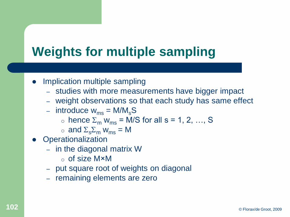
Weights for multiple sampling
Implication multiple sampling
– studies with more measurements have bigger impact
– weight observations so that each study has same effect
– introduce wms = M/MsS
o hence Sm wms = M/S for all s = 1, 2, …, S
o and SsSm wms = M
Operationalization
– in the diagonal matrix W
o of size M×M
– put square root of weights on diagonal
– remaining elements are zero
© Florax/de Groot, 2009103
Software
Tailored software (watch out for applicability)
Macros of general packages for ―classical‖ analysis
- SAS (Arthur et al., 2001, Conducting meta-analysis using Sas)
- Stata (see newsletter)
- R (meta scripts)
WinBUGS for Bayesian analysis
General software
- Eviews, Limdep, SPSS, etc.