Message-passing for graph-structured linearprograms: Proximal methods and rounding schemes

Pradeep Ravikumar† Alekh Agarwal!

pradeepr@stat.berkeley.edu alekh@eecs.berkeley.edu

Martin J. Wainwright†,!

wainwrig@stat.berkeley.edu

Department of Statistics†, andDepartment of Electrical Engineering and Computer Sciences!

University of California, BerkeleyBerkeley, CA 94720

October 17, 2008

Abstract

The problem of computing a maximum a posteriori (MAP) configuration is a centralcomputational challenge associated with Markov random fields. A line of work has focusedon “tree-based” linear programming (LP) relaxations for the MAP problem. This paperdevelops a family of super-linearly convergent algorithms for solving these LPs, based onproximal minimization schemes using Bregman divergences. As with standard message-passing on graphs, the algorithms are distributed and exploit the underlying graphicalstructure, and so scale well to large problems. Our algorithms have a double-loop char-acter, with the outer loop corresponding to the proximal sequence, and an inner loop ofcyclic Bregman divergences used to compute each proximal update. Di!erent choices ofthe Bregman divergence lead to conceptually related but distinct LP-solving algorithms.We establish convergence guarantees for our algorithms, and illustrate their performancevia some simulations. We also develop two classes of graph-structured rounding schemes,randomized and deterministic, for obtaining integral configurations from the LP solu-tions. Our deterministic rounding schemes use a “re-parameterization” property of ouralgorithms so that when the LP solution is integral, the MAP solution can be obtainedeven before the LP-solver converges to the optimum. We also propose a graph-structuredrandomized rounding scheme that applies to iterative LP solving algorithms in general.We analyze the performance of our rounding schemes, giving bounds on the number ofiterations required, when the LP is integral, for the rounding schemes to obtain the MAPsolution. These bounds are expressed in terms of the strength of the potential functions,and the energy gap, which measures how well the integral MAP solution is separatedfrom other integral configurations. We also report simulations comparing these roundingschemes.

1 Introduction

A key computational challenge that arises in applications of discrete graphical models is tocompute the most probable configuration(s), often referred to as the maximum a posteriori(MAP) problem. Although the MAP problem can be solved exactly in polynomial time ontrees (and more generally, graphs with bounded treewidth) using the max-product algorithm,it is computationally challenging for general graphs. Indeed, the MAP problem for generaldiscrete graphical models includes a large number of classical NP-complete problems as specialcases, including MAX-CUT, independent set, and various satisfiability problems.

1

This intractability motivates the development and analysis of methods for obtaining ap-proximate solutions, and there is a long history of approaches to the problem. One class ofmethods is based on simulated annealing (Geman and Geman, 1984), but the cooling schedulesrequired for theoretical guarantees are often prohibitively slow. Besag (1986) proposed the it-erated conditional modes algorithm, which performs a sequence of greedy local maximizationsto approximate the MAP solution, but may be trapped by local maxima. Greig et al. (1989)observed that for binary problems with attractive pairwise interactions (the ferromagneticIsing model in statistical physics terminology), the MAP configuration can be computed inpolynomial-time by reduction to a max-flow problem. The ordinary max-product algorithm,a form of non-serial dynamic-programming (Bertele and Brioschi, 1972), computes the MAPconfiguration exactly for trees, and is also frequently applied to graphs with cycles. Despitesome local optimality results (Freeman and Weiss, 2001; Wainwright et al., 2004), it has nogeneral correctness guarantees for graph with cycles, and even worse, it can converge rapidlyto non-MAP configurations (Wainwright et al., 2005), even for problems that are easily solvedin polynomial time (e.g., ferromagnetic Ising models). For certain graphical models arisingin computer vision, Boykov et al. (2001) proposed graph-cut based search algorithms thatcompute a local maximum over two classes of moves. A broad class of methods are based onthe principle of convex relaxation, in which the discrete MAP problem is relaxed to a convexoptimization problem over continuous variables. Examples of this convex relaxation probleminclude linear programming relaxations (Koval and Schlesinger, 1976; Chekuri et al., 2005;Wainwright et al., 2005), as well as quadratic, semidefinite and other conic programming re-laxations (for instance, (Ravikumar and La!erty, 2006; Kumar et al., 2006; Wainwright andJordan, 2004)).

Among the family of conic programming relaxations, linear programming (LP) relaxationis the least expensive computationally, and also the best understood. The primary focus ofthis paper is a well-known LP relaxation of the MAP estimation problem for pairwise Markovrandom fields, one which has been independently proposed by several groups (Koval andSchlesinger, 1976; Chekuri et al., 2005; Wainwright et al., 2005). This LP relaxation is basedon optimizing over a set of locally consistent pseudomarginals on edges and vertices of thegraph. It is an exact method for any tree-structured graph, so that it can be viewed naturallyas a tree-based LP relaxation.1 The first connection between max-product message-passingand LP relaxation was made by Wainwright et al. (2005), who connected the tree-based LPrelaxation to the class of tree-reweighted max-product (TRW-MP) algorithms, showing thatTRW-MP fixed points satisfying a strong “tree agreement” condition specify optimal solutionsto the LP relaxation.

For general graphs, this first-order LP relaxation could be solved—at least in principle—byvarious standard algorithms for linear programming, including the simplex and interior-pointmethods (Bertsimas and Tsitsikilis, 1997; Boyd and Vandenberghe, 2004). However, suchgeneric methods fail to exploit the graph-structured nature of the LP, and hence do notscale favorably to large-scale problems (Yanover et al., 2006). A body of work has extendedthe connection between the LP relaxation and message-passing algorithms in various ways.Kolmogorov (2005) developed a serial form of TRW-MP updates with certain convergenceguarantees; he also showed that there exist fixed points of the TRW-MP algorithm, notsatisfying strong tree agreement, that do not correspond to optimal solutions of the LP.This issue has a geometric interpretation, related to the fact that co-ordinate ascent schemes

1In fact, this LP relaxation is the first in a hierarchy of relaxations, based on the treewidth of thegraph (Wainwright et al., 2005).

2

(to which TRW-MP is closely related), need not converge to the global optima for convexprograms that are not strictly convex, but can become trapped in corners. Kolmogorov andWainwright (2005) showed that this trapping phenomena does not arise for graphical modelswith binary variables and pairwise interactions, so that TRW-MP fixed points are alwaysLP optimal. Globerson and Jaakkola (2007) developed a related but di!erent dual-ascentalgorithm, which is guaranteed to converge but is not guaranteed to solve the LP. Weisset al. (2007) established connections between convex forms of the sum-product algorithm,and exactness of reweighted max-product algorithms; Johnson et al. (2007) also proposedalgorithms related to convex forms of sum-product. Various authors have connected theordinary max-product algorithm to the LP relaxation for special classes of combinatorialproblems, including matching (Bayati et al., 2005; Huang and Jebara, 2007; Bayati et al., 2007)and independent set (Sanghavi et al., 2007). For general problems, max-product does notsolve the LP; Wainwright et al. (2005) describe a instance of the MIN-CUT problem on whichmax-product fails, even though LP relaxation is exact. Other authors (Feldman et al., 2002;Komodakis et al., 2007) have implemented subgradient methods which are guaranteed to solvethe linear program, but such methods typically have sub-linear convergence rates (Bertsimasand Tsitsikilis, 1997).

This paper makes two contributions to this line of work. Our first contribution is todevelop and analyze a class of message-passing algorithms with the following properties: theironly fixed points are LP-optimal solutions, they are provably convergent with at least ageometric rate, and they have a distributed nature, respecting the graphical structure of theproblem. All of the algorithms in this paper are based on the well-established idea of proximalminimization: instead of directly solving the original linear program itself, we solve a sequenceof so-called proximal problems, with the property that the sequence of associated solutionsis guaranteed to converge to the LP solution. We describe di!erent classes of algorithms,based on di!erent choices of the proximal function: quadratic, entropic, and tree-reweightedentropies. For all choices, we show how the intermediate proximal problems can be solvedby forms of message-passing on the graph—similar to but distinct from the ordinary max-product or sum-product updates. An additional desirable feature, given the wide variety oflifting methods for further constraining LP relaxations (Wainwright and Jordan, 2003), isthat new constraints can be incorporated in a relatively seamless manner, by introducing newmessages to enforce them.

Our second contribution is to develop various types of rounding schemes that allow for earlytermination of LP-solving algorithms. There is a substantial body of past work (e.g., (Ragha-van and Thompson, 1987)) on rounding fractional LP solutions so as to obtain an integralsolutions with approximation guarantees. Our use of rounding is rather di!erent: instead, weconsider rounding schemes applied to problems for which the LP solution is integral, so thatrounding would be unnecessary if the LP were solved to optimality. In this setting, the benefitof certain rounding procedures (in particular, those that we develop) is allowing an LP-solvingalgorithm to be terminated before it has solved the LP, while still returning the MAP configu-ration, either with a deterministic or high probability guarantee. Our deterministic roundingschemes apply to a class of algorithms which, like the proximal minimization algorithms thatwe propose, maintain a certain invariant of the original problem. We also propose and analyzea class of graph-structured randomized rounding procedures that apply to any algorithm thatapproaches the optimal LP solution from the interior of the relaxed polytope. We analyzethese rounding schemes, and give finite bounds on the number of iterations required for therounding schemes to obtain an integral MAP solution.

The remainder of this paper is organized as follows. We begin in Section 2 with background

3

on Markov random fields, and the first-order LP relaxation. In Section 3, we introduce thenotions of proximal minimization and Bregman divergences, then derive various of message-passing algorithms based on these notions, and finally discuss their convergence properties.Section 4 is devoted to the development and analysis of rounding schemes, both for ourproximal schemes as well as other classes of LP-solving algorithms. We provide experimentalresults in Section 5, and conclude with a discussion in Section 6.

2 Background

We begin by introducing some background on Markov random fields, and the LP relax-ations that are the focus of this paper. Given a discrete space X = {0, 1, 2, . . . ,m ! 1}, letX = (X1, . . . ,XN ) " XN denote a N -dimensional discrete random vector. We assume thatits distribution P is a Markov random field, meaning that it factors according to the structureof an undirected graph G = (V,E), with each variable Xs associated with one node s " V ,in the following way. Letting !s : X # R and !st : X $ X # R be singleton and edgewisepotential functions respectively, we assume that the distribution takes the form

P(x; !) % exp! "

s!V

!s(xs) +"

(s,t)!E

!st(xs, xt)#.

The problem of maximum a posteriori (MAP) estimation is to compute a configurationwith maximum probability—i.e., an element

x" " arg maxx!XN

! "

s!V

!s(xs) +"

(s,t)!E

!st(xs, xt)#, (1)

where the arg max operator extracts the configurations that achieve the maximal value. Thisproblem is an integer program, since it involves optimizing over the discrete space XN . Forfuture reference, we note that the functions !s(·) and !st(·) can always be represented in theform

!s(xs) ="

j!X

!s;jI[xs = j] (2a)

!st(xs, xt) ="

j,k!X

!st;jkI[xs = j; xt = k], (2b)

where the m-vectors {!s;j, j " X} and m $ m matrices {!st;jk, (j, k) " X $ X} parameterizethe problem.

The first-order linear programming (LP) relaxation (Koval and Schlesinger, 1976; Chekuriet al., 2005; Wainwright et al., 2005) of this problem is based on a set of pseudomarginalsµs and µst, associated with the nodes and vertices of the graph. These pseudomarginals areconstrained to be non-negative, as well to normalize and be locally consistent in the followingsense:

"

xs!X

µs(xs) = 1, for all s " V , and (3a)

"

xt!X

µst(xs, xt) = µs(xs) for all (s, t) " E, xs " X . (3b)

4

The polytope defined by the non-negativity constraints µ & 0, the normalization constraints (3a)and the marginalization constraints (3b), is denoted by L(G). The LP relaxation is based onmaximizing the linear function

'!, µ( : ="

s!V

"

xs

!s(xs)µs(xs) +"

(s,t)!E

"

xs,xt

!st(xs, xt)µst(xs, xt), (4)

subject to the constraint µ " L(G).In the sequel, we write the linear program (4) more compactly in the form maxµ!L(G)'!, µ(.

By construction, this relaxation is guaranteed to be exact for any problem on a tree-structuredgraph (Wainwright et al., 2005), so that it can be viewed as a tree-based relaxation. Themain goal of this paper is to develop e"cient and distributed algorithms for solving thisLP relaxation, as well as strengthenings based on additional constraints. For instance, onenatural strengthening is by “lifting”: view the pairwise MRF as a particular case of a moregeneral MRF with higher order cliques, define higher-order pseudomarginals on these cliques,and use them to impose higher-order consistency constraints. This particular progression oftighter relaxations underlies the Bethe to Kikuchi (sum-product to generalized sum-product)hierarchy (Yedidia et al., 2005); see Wainwright and Jordan (2003) for further discussion ofsuch LP hierarchies.

3 Proximal minimization schemes

We begin by defining the notion of a proximal minimization scheme, and various types ofdivergences (among them Bregman) that we use to define our proximal sequences. Insteadof dealing with the maximization problem maxµ!L(G)'!, µ(, it is convenient to consider theequivalent minimization problem minµ!L(G) !'!, µ(.

3.1 Proximal minimization

The class of methods that we develop are based on the notion of proximal minimization (Bert-sekas and Tsitsiklis, 1997). Instead of attempting to solve the LP directly, we solve a sequenceof problems of the form

µn+1 = arg minµ!L(G)

$! '!, µ( +

1

"nDf (µ )µn)

%, (5)

where for iteration numbers n = 0, 1, 2, . . ., the vector µn denotes current iterate, the quantity"n is a positive weight, and Df is a generalized distance function, known as the proximalfunction. (Note that we are using superscripts to represent the iteration number, not for thepower operation.)

The purpose of introducing the proximal function is to convert the original LP—which isconvex but not strictly so—into a strictly convex problem. The latter property is desirable fora number of reasons. First, for strictly convex programs, co-ordinate descent schemes are guar-anteed to converge to the global optimum; note that they may become trapped for non-strictlyconvex problems, such as the piecewise linear surfaces that arise in linear programming. More-over, the dual of a strictly convex problem is guaranteed to be di!erentiable (Bertsekas, 1995);a guarantee which need not hold for non-strictly convex problems. Note that di!erentiabledual functions can in general be solved more easily than non-di!erentiable dual functions. In

5

the sequel, we show how for appropriately chosen generalized distances, the proximal sequence{µn} can be computed using message passing updates derived from cyclic projections.

We note that the proximal scheme (5) is similar to an annealing scheme, in that it involvesperturbing the original cost function, with a choice of weights {"n}. While the weights{"n} can be adjusted for faster convergence, they can also be set to a constant, unlike forstandard annealing procedures in which the annealing weight is taken to 0. The reason is thatDf (µ )µ(n)), as a generalized distance, itself converges to zero as the algorithm approachesthe optimum, thus providing an “adaptive” annealing. For appropriate choice of weights andproximal functions, these proximal minimization schemes converge to the LP optimum withat least geometric and possibly superlinear rates (Bertsekas and Tsitsiklis, 1997; Iusem andTeboulle, 1995).

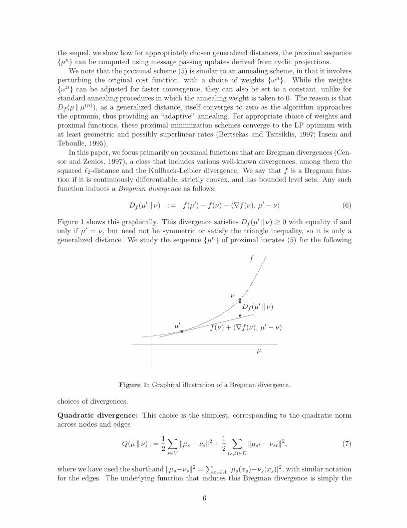
In this paper, we focus primarily on proximal functions that are Bregman divergences (Cen-sor and Zenios, 1997), a class that includes various well-known divergences, among them thesquared #2-distance and the Kullback-Leibler divergence. We say that f is a Bregman func-tion if it is continuously di!erentiable, strictly convex, and has bounded level sets. Any suchfunction induces a Bregman divergence as follows:

Df (µ# ) $) := f(µ#) ! f($) ! '*f($), µ# ! $( (6)

Figure 1 shows this graphically. This divergence satisfies Df (µ# ) $) & 0 with equality if andonly if µ# = $, but need not be symmetric or satisfy the triangle inequality, so it is only ageneralized distance. We study the sequence {µn} of proximal iterates (5) for the following

f

µ#

$

µ

Df (µ# ) $)

f($) + '*f($), µ# ! $(

Figure 1: Graphical illustration of a Bregman divergence.

choices of divergences.

Quadratic divergence: This choice is the simplest, corresponding to the quadratic normacross nodes and edges

Q(µ ) $) :=1

2

"

s!V

)µs ! $s)2 +1

2

"

(s,t)!E

)µst ! $st)2, (7)

where we have used the shorthand )µs!$s)2 =&

xs!X |µs(xs)!$s(xs)|2, with similar notationfor the edges. The underlying function that induces this Bregman divergence is simply the

6

quadratic function

q(µ) :=1

2

$ "

s!V

"

xs!X

µ2s(xs) +

"

(s,t)!E

"

(xs,xt)!X$X

µ2st(xs, xt)

%, (8)

defined over nodes and edges of the graph.

Weighted entropic divergence: Another Bregman divergence can be defined by theweighted sum of Kullback-Leibler (KL) divergences across the nodes and edges. In par-ticular, letting %s > 0 and %st > 0 be positive weights associated with node s and edge (s, t)respectively, we define

D"(µ ) $) ="

s!V

%sD(µs ) $s) +"

(s,t)!E

%stD(µst ) $st), (9)

where D(p ) q) :=&

x

'p(x) log p(x)

q(x) !(p(x) ! q(x)

)*is the KL divergence. An advantage of

the KL divergence, relative to the quadratic norm, is that it automatically acts to enforce non-negativity constraints on the pseudomarginals in the proximal minimization problem. (SeeSection 3.4 for a more detailed discussion of this issue.) The associated Bregman function isweighted sum of entropies

h"(µ) ="

s!V

%sHs(µs) +"

(s,t)!E

%stHst(µst), (10)

where Hs and Hst are defined by

Hs(µs) :="

xs!X

µs(xs) log µs(xs), and

Hst(µst) :="

(xs,xt)!X$X

µst(xs, xt) log µst(xs, xt),

corresponding to node-based and edge-based entropies, respectively.

Tree-reweighted entropic divergence: Our last example is a divergence obtained from aconvex combination of tree-structured entropies (Wainwright and Jordan, 2003). In particular,given a weight &st " (0, 1] for each edge (s, t) of the graph, we define

f#(µ) :="

s!V

Hs(µs) !"

(s,t)!E

&stIst(µst). (11)

In this definition, the quantity

Ist(µst) :="

(xs,xt)!X$X

µst(xs, xt) logµst(xs, xt)

[&

x!

tµst(xs, x#

t)][&

x!sµst(x#

s, xt)](12)

is the mutual information associated with edge (s, t). It can be shown that this function isstrictly convex when restricted to µ " L(G). If µ " L(G), then the divergence induced by thefunction (11) is related to weighted entropy family (10), except that the node entropy weights%s are not always positive.

7

3.2 Proximal sequences via Bregman projection

The key in designing an e"cient proximal minimization scheme is ensuring that the proximalsequence {µn} can be computed e"ciently. In this section, we first describe how sequences ofproximal minimizations (when the proximal function is a Bregman divergence) can be refor-mulated as a particular Bregman projection. We then describe how this Bregman projectioncan itself be computed iteratively, in terms of a sequence of cyclic Bregman projections (Cen-sor and Zenios, 1997) based on a decomposition of the constraint set L(G). In the sequel,we then show how this cyclic Bregman projections reduce to very simple message-passingupdates.

Given a Bregman divergence D, the Bregman projection of the vector $ onto a convex setC is given by

+µ : = arg minµ!C

Df (µ ) $) (13)

By taking derivatives and using standard conditions for optima over convex sets (Bertsekas,1995), the defining optimality condition for +µ is

'*f(+µ) !*f($), µ ! +µ( & 0 (14)

for all µ " C. Now consider the proximal minimization problem to be solved at step n, namelythe strictly convex problem

minµ!L(G)

$! '!, µ( +

1

"nDf (µ )µn)

%. (15)

By taking derivatives and using the same convex optimality, we see that the optimum µn+1

is defined by the conditions

'*f(µn+1) !*f(µn) ! "n!, µ ! µn+1( & 0

for all µ " C. Note that these optimality conditions are of the same form as the Bregmanprojection conditions (14), with the vector *f(µn) + "n! taking the role of *f($); in otherwords, with (*f)%1(*f(µ)+"n!) being substituted for $. Consequently, e"cient algorithmsfor computing the Bregman projection (14) can be leveraged to compute the proximal up-date (15). In particular, our algorithms leverage the fact that Bregman projections can becomputed e"ciently in a cyclic manner—that is, by decomposing the constraint set C = +iCi

into an intersection of simpler constraint sets, and then performing a sequence of projectionsonto these simple constraint sets (Censor and Zenios, 1997).

To simplify notation, for any Bregman function f , induced divergence Df , and convexset C, let us define the operator Jf (µ, $) := (*f)%1(*f(µ) + $), as well as the projectionoperator

#f (';C) := arg minµ!C

Df (µ ) ').

With this notation, we can write the proximal update in a compact manner as the compoundedoperation

µn+1 = #f

,Jf (µn,"n!); L(G)

-.

Now consider a decomposition of the constraint set as an intersection—say L(G) = +Tk=1Lk(G).

By the method of cyclic Bregman projections (Censor and Zenios, 1997), we can compute

8

µn+1 in an iterative manner, by performing the sequence of projections onto the simplerconstraint sets, initializing µn,0 = µn and updating from µn,$ ,# µn,$+1 by projecting µn,$

onto constraint set Li($)(G), where i(() = ( mod T , for instance. This meta-algorithm issummarized in Algorithm 1.

Algorithm 1 Basic proximal-Bregman LP solver

Given a Bregman distance D, weight sequence {"n} and problem parameters !:

• Initialize µ0 to the uniform distribution: µ(0)s (xs) = 1

m , µ(0)st (xs, xt) = 1

m2 .

• Outer Loop: For iterations n = 0, 1, 2, . . ., update µn+1 = #f

,Jf (µn,"n!); L(G)

-.

– Solve Outer Loop via Inner Loop:

(a) Inner initialization µn,0 = Jf (µn,"n!).

(b) For t = 0, 1, 2, . . ., set i(t) = t mod T .

(c) Update µn,t+1 = #f

,µn,t; Li(t)(G)

-.

As shown in the following sections, by using a decomposition of L(G) over the edges of thegraph, the inner loop steps correspond to local message-passing updates, slightly di!erent innature depending on the choice of Bregman distance. Iterating the inner and outer loops yieldsa provably convergent message-passing algorithm for the LP. Convergence follows from theconvergence properties of proximal minimization (Bertsekas and Tsitsiklis, 1997), combinedwith convergence guarantees for cyclic Bregman projections (Censor and Zenios, 1997). In thefollowing section, we derive the message-passing updates corresponding to various Bregmanfunctions of interest.

3.3 Quadratic Projections

Consider the proximal sequence with the quadratic distance Q from equation (7); the Bregmanfunction inducing this distance is the quadratic function q(y) = 1

2y2, with gradient *q(y) = y.A little calculation shows that the operator Jq takes the form

Jq(µ,"!) = µ + "!, (16)

whence we obtain the initialization in equation (18a).We now turn to the projections µn,$+1 = #q(µn,$ , Li(G)) onto the individual constraints

Li(G). For each such constraint, the local update is based on the solving the problem

µn,$+1 = arg min%!Li(G)

$q($) ! '$, *q(µn,$ )(

%. (17)

In Appendix A.1, we show how the solution to these inner updates takes the form (19a) givenin Algorithm (2).

3.4 Entropic projections

Consider the proximal sequence with the Kullback-Leibler distance D(µ ) $) defined in equa-tion (9). The Bregman function h" inducing the distance is a sum of negative entropy functions

9

Algorithm 2 Quadratic Messages for µn+1

Initialization:

µ(n,0)st (xs, xt) = µ(n)

st (xs, xt) + wn!st(xs, xt) (18a)

µ(n,0)s (xs) = µ(n)

s (xs) + wn!s(xs) (18b)

repeat

for each edge (s, t) " E do

µ(n,!+1)st (xs, xt) = max

.

µ(n,!)st (xs, xt) +

,1

L + 1

-,µ(n,!)

s (xs) !"

xt

µ(n,!)st (xs, xt)

-, 0

/

(19a)

µ(n,!+1)s (xs) = µ(n,!)

s (xs) +

,1

L + 1

-,! µ(n,!)

s (xs) +"

xt

µ(n,!)st (xs, xt)

-(19b)

end for

for each node s " V do

µ(n,!+1)s (xs) = max

$0, µ(n,!)

s (xs) +1

L

0

1 !"

xs

µ(n,!)s (xs)

1%(20)

end for

until convergence

f(µ) = µ log µ, and its gradient is given by *f(µ) = log(µ)+)1. In this case, some calculationshows that the map $ = Jf (µ,"!) is given by

*f($) = µ exp("!),

whence we obtain the initialization equation (21a). In Appendix A.2, we derive the message-passing updates summarized in Algorithm (3).Remark: In the special case of uniformly weighted entropies (i.e., %s = %st = 1), it is worthnoting that the updates of Algorithm (3) are reminiscent of the junction tree algorithm (Lau-ritzen, 1996), which also update the marginals {µs, µst}, or primal parameters directly.

3.5 Tree-reweighted entropy proximal sequences

In the previous sections, we saw how to solve the proximal sequences using message passingupdates derived from cyclic Bregman projections. In this section, we show that for thetree-reweighted entropy divergence, we can also use tree-reweighted sum-product or relatedmethods (Globerson and Jaakkola, 2007; Hazan and Shashua, 2008) to compute the proximalsequence. We first rewrite the proximal sequence optimization problem (5) as

µn+1 = arg min%!L(G)

$! '"! + *f#(µ

n), $( ! f#($)

%. (25)

Computing the gradient of the function f#, and performing some algebra yields the algorithmictemplate of Algorithm 4. With this particular choice of proximal function, the resultingalgorithm can be understood as approaching the zero-temperature limit of the tree-reweighted

10

Algorithm 3 Entropic Messages for µn+1

Initialization:

µ(n,0)st (xs, xt) = µ(n)

st (xs, xt) exp("n!st(xs, xt)/%st), and (21a)

µ(n,0)s (xs) = µ(n)

s (xs) exp("n !s(xs)/%s). (21b)

repeat

for each edge (s, t) " E do

µ(n,$+1)st (xs, xt) = µ(n,$)

st (xs, xt)

,µ(n,$)

s (xs)&

xtµ(n,$)

st (xs, xt)

- !s

!s+!st

, and (22)

µ(n,$+1)s (xs) = µ(n,$)

s (xs)!s

!s+!st

, "

xt

µ(n,$)st (xs, xt)

- !st

!s+!st

(23)

end for

for each node s " V do

µ(n,$+1)s (xs) =

µ(n,$)s (xs)

&xs

µ(n,$)s (xs)

(24)

end for

until convergence

Bethe problem; by convexity, the optimizers of this sequence are guaranteed to approach theLP optima (Wainwright and Jordan, 2003). Moreover, as pointed by Weiss et al. (2007),various other convexified entropies (in addition to the tree-reweighted one) also have thisproperty.

3.6 Convergence

We now turn to the convergence of the message-passing algorithms that we have proposed.At a high-level, for any Bregman proximal function, convergence follows from two sets ofknown results: (a) convergence of proximal algorithms; and (b) convergence of cyclic Bregmanprojections.

For completeness, we re-state the consequences of these results here. For any positivesequence "n > 0, we say that it satisfies the infinite travel condition if

&&n=1(1/"

n) = +-.We let µ" " L(G) denote an optimal solution (not necessarily unique) of the LP, and usef" = f(µ") = '!, µ"( to denote the LP optimal value. We say that the convergence rate issuperlinear if

limn'+&

|f(µn+1) ! f"||f(µn) ! f"| = 0, (29)

and linear if

limn'+&

|f(µn+1) ! f"||f(µn) ! f"| . ', (30)

11

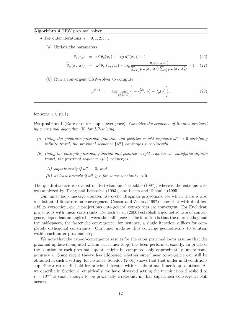
Algorithm 4 TRW proximal solver

• For outer iterations n = 0, 1, 2, . . .,

(a) Update the parameters:

2!s(xs) = "n!s(xs) + log(µn(xs)) + 1 (26)

2!st(xs, xt) = "n!st(xs, xt) + logµst(xs, xt)&

x!sµst(x#

s, xt)&

x!

tµst(xs, x#

t)! 1 (27)

(b) Run a convergent TRW-solver to compute

µn+1 = arg min%!L(G)

$! '2!n, $( ! f#($)

%. (28)

for some ' " (0, 1).

Proposition 1 (Rate of outer loop convergence). Consider the sequence of iterates producedby a proximal algorithm (5) for LP-solving.

(a) Using the quadratic proximal function and positive weight sequence "n # 0 satisfyinginfinite travel, the proximal sequence {µn} converges superlinearly.

(b) Using the entropic proximal function and positive weight sequence "n satisfying infinitetravel, the proximal sequence {µn} converges:

(i) superlinearly if "n # 0, and

(ii) at least linearly if "n & c for some constant c > 0.

The quadratic case is covered in Bertsekas and Tsitsiklis (1997), whereas the entropic casewas analyzed by Tseng and Bertsekas (1993), and Iusem and Teboulle (1995).

Our inner loop message updates use cyclic Bregman projections, for which there is alsoa substantial literature on convergence. Censor and Zenios (1997) show that with dual fea-sibility correction, cyclic projections onto general convex sets are convergent. For Euclideanprojections with linear constraints, Deutsch et al. (2006) establish a geometric rate of conver-gence, dependent on angles between the half-spaces. The intuition is that the more orthogonalthe half-spaces, the faster the convergence; for instance, a single iteration su"ces for com-pletely orthogonal constraints. Our inner updates thus converge geometrically to solutionwithin each outer proximal step.

We note that the rate-of-convergence results for the outer proximal loops assume that theproximal update (computed within each inner loop) has been performed exactly. In practice,the solution to each proximal update might be computed only approximately, up to someaccuracy *. Some recent theory has addressed whether superlinear convergence can still beobtained in such a setting; for instance, Solodov (2001) shows that that under mild conditionssuperlinear rates still hold for proximal iterates with *!suboptimal inner-loop solutions. Aswe describe in Section 5, empirically, we have observed setting the termination threshold to* = 10%6 is small enough to be practically irrelevant, in that superlinear convergence stilloccurs.

12

4 Rounding with optimality guarantees

Recall that the graph-structured LP (4) is a relaxation of the MAP integer program, so thatthere are two possible outcomes to solving the LP: either an integral vertex is obtained, whichis then guaranteed to be a MAP configuration, or a fractional vertex is obtained, in whichcase the relaxation is loose. In the latter case, a natural strategy is to “round” the fractionalsolution, so as to obtain an integral solution (Raghavan and Thompson, 1987). Such roundingschemes may either be randomized or deterministic. A natural measure of the quality of therounded solution is in terms of its value relative to the optimal (MAP) value. There is now asubstantial literature on performance guarantees of various rounding schemes, when appliedto particular sub-classes of MAP problems (e.g., (Raghavan and Thompson, 1987; Kleinbergand Tardos, 1999; Chekuri et al., 2005)).

In this section, we show that rounding schemes can be useful even when the LP optimumis integral, since they may permit an LP-solving algorithm to be finitely terminated—i.e.,before it has actually solved the LP—while retaining the same optimality guarantees aboutthe final output. An attractive feature of our proximal Bregman procedures is the existenceof precisely such rounding schemes–namely, that under certain conditions, rounding pseu-domarginals at intermediate iterations yields the integral LP optimum. In Section 4.1, wedescribe deterministic rounding schemes that apply to the proximal Bregman procedures thatwe have described; moreover, we provide upper bounds on the number of outer iterationsrequired for the rounding scheme to obtain the LP optimum. In Section 4.2, we propose andanalyze a graph-structured randomized rounding scheme, which applies not only to proximalBregman procedures, but more broadly to any algorithm that generates a sequence of iteratescontained within the local polytope L(G).

4.1 Deterministic rounding schemes

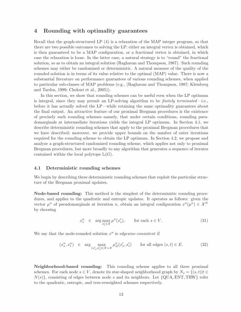
We begin by describing three deterministic rounding schemes that exploit the particular struc-ture of the Bregman proximal updates.

Node-based rounding: This method is the simplest of the deterministic rounding proce-dures, and applies to the quadratic and entropic updates. It operates as follows: given thevector µn of pseudomarginals at iteration n, obtain an integral configuration xn(µn) " XN

by choosing

xns " arg max

x!s!X

µn(x#s), for each s " V . (31)

We say that the node-rounded solution xn is edgewise-consistent if

(xns , xn

t ) " arg max(x!

s,x!

t)!X$X

µnst(x

#s, x

#t) for all edges (s, t) " E. (32)

Neighborhood-based rounding: This rounding scheme applies to all three proximalschemes. For each node s " V , denote its star-shaped neighborhood graph by Ns = {(s, t)|t "N(s)}, consisting of edges between node s and its neighbors. Let {QUA,ENT,TRW} referto the quadratic, entropic, and tree-reweighted schemes respectively.

13

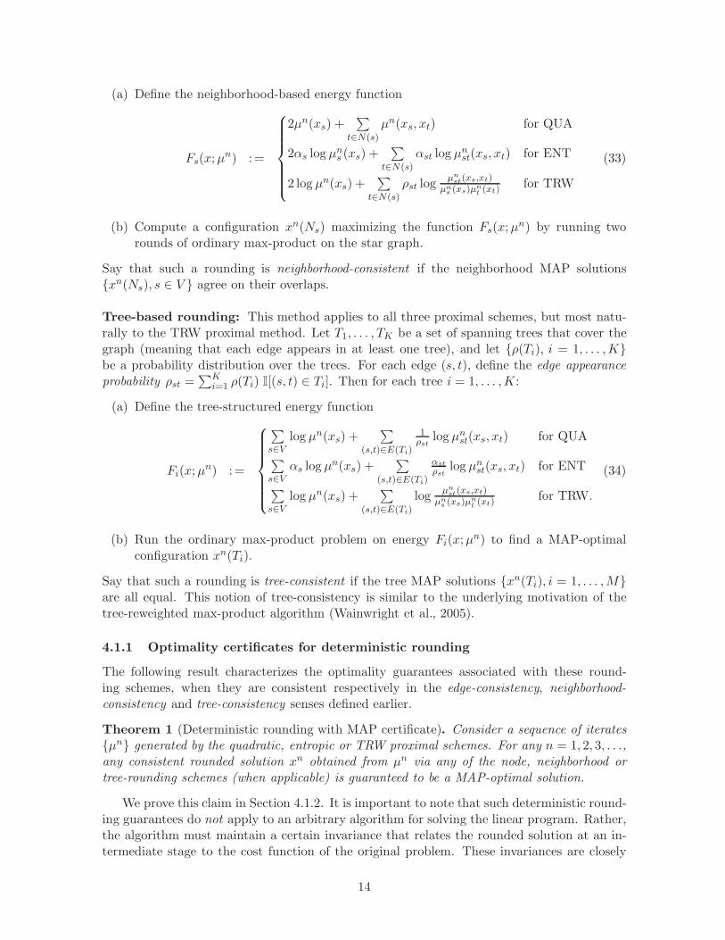
(a) Define the neighborhood-based energy function

Fs(x;µn) :=

3444445

444446

2µn(xs) +&

t!N(s)µn(xs, xt) for QUA

2%s log µns (xs) +

&

t!N(s)%st log µn

st(xs, xt) for ENT

2 log µn(xs) +&

t!N(s)&st log µn

st(xs,xt)µn

s (xs)µnt(xt)

for TRW

(33)

(b) Compute a configuration xn(Ns) maximizing the function Fs(x;µn) by running tworounds of ordinary max-product on the star graph.

Say that such a rounding is neighborhood-consistent if the neighborhood MAP solutions{xn(Ns), s " V } agree on their overlaps.

Tree-based rounding: This method applies to all three proximal schemes, but most natu-rally to the TRW proximal method. Let T1, . . . , TK be a set of spanning trees that cover thegraph (meaning that each edge appears in at least one tree), and let {&(Ti), i = 1, . . . ,K}be a probability distribution over the trees. For each edge (s, t), define the edge appearanceprobability &st =

&Ki=1 &(Ti) I[(s, t) " Ti]. Then for each tree i = 1, . . . ,K:

(a) Define the tree-structured energy function

Fi(x;µn) :=

3444445

444446

&

s!Vlog µn(xs) +

&

(s,t)!E(Ti)

1#st

log µnst(xs, xt) for QUA

&

s!V%s log µn(xs) +

&

(s,t)!E(Ti)

"st

#stlog µn

st(xs, xt) for ENT

&

s!Vlog µn(xs) +

&

(s,t)!E(Ti)log µn

st(xs,xt)µn

s (xs)µnt(xt)

for TRW.

(34)

(b) Run the ordinary max-product problem on energy Fi(x;µn) to find a MAP-optimalconfiguration xn(Ti).

Say that such a rounding is tree-consistent if the tree MAP solutions {xn(Ti), i = 1, . . . ,M}are all equal. This notion of tree-consistency is similar to the underlying motivation of thetree-reweighted max-product algorithm (Wainwright et al., 2005).

4.1.1 Optimality certificates for deterministic rounding

The following result characterizes the optimality guarantees associated with these round-ing schemes, when they are consistent respectively in the edge-consistency, neighborhood-consistency and tree-consistency senses defined earlier.

Theorem 1 (Deterministic rounding with MAP certificate). Consider a sequence of iterates{µn} generated by the quadratic, entropic or TRW proximal schemes. For any n = 1, 2, 3, . . .,any consistent rounded solution xn obtained from µn via any of the node, neighborhood ortree-rounding schemes (when applicable) is guaranteed to be a MAP-optimal solution.

We prove this claim in Section 4.1.2. It is important to note that such deterministic round-ing guarantees do not apply to an arbitrary algorithm for solving the linear program. Rather,the algorithm must maintain a certain invariance that relates the rounded solution at an in-termediate stage to the cost function of the original problem. These invariances are closely

14

related to the reparameterization condition satisfied by the sum-product algorithm (Wain-wright et al., 2003).

All of the rounding schemes require relatively little computation. The node-roundingscheme is trivial to implement. The neighborhood-based scheme requires running two itera-tions of max-product for each neighborhood of the graph. Finally, the tree-rounding schemerequires O(KN) iterations of max-product, where K is the number of trees that cover thegraph, and N is the number of nodes. Many graphs with cycles can be covered with a smallnumber K of trees; for instance, the lattice graph in 2-dimensions can be covered with twospanning trees, in which case the rounding cost is linear in the number of nodes.

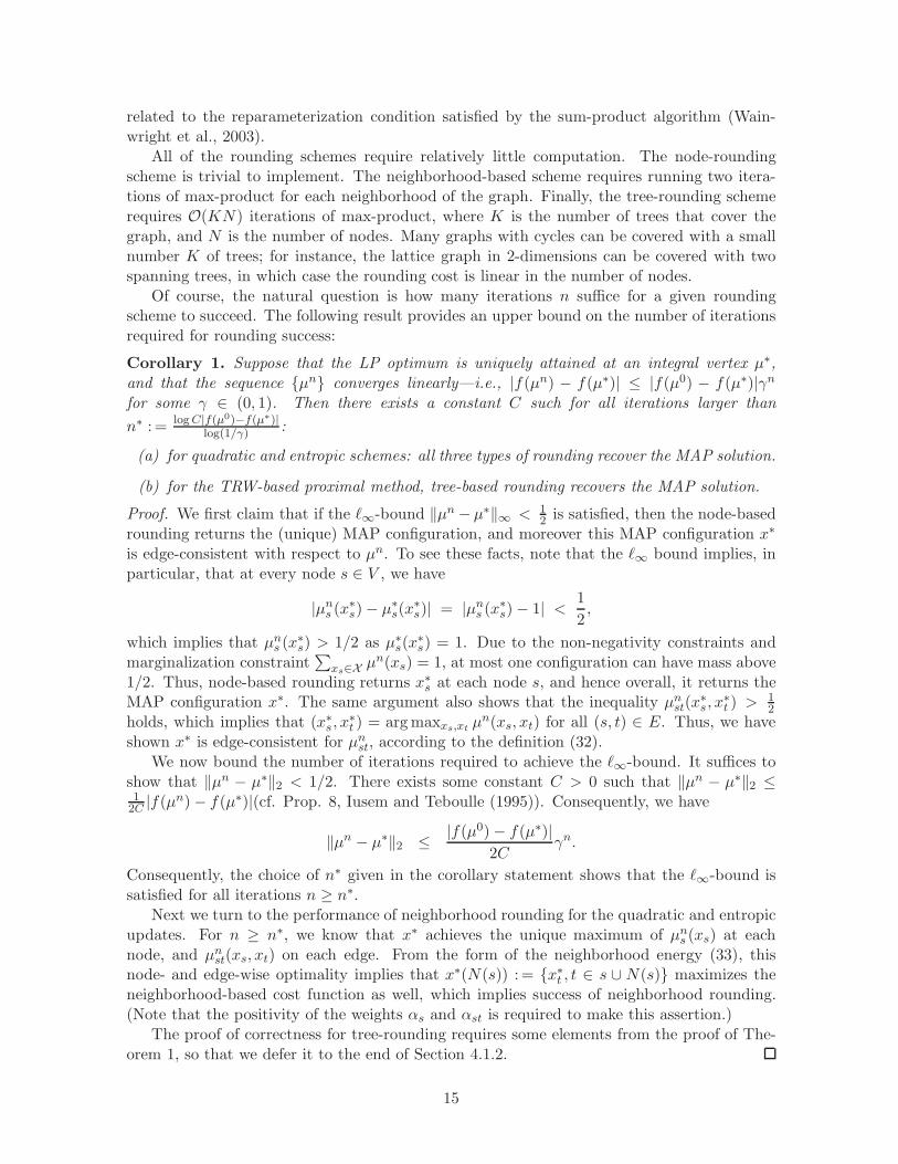
Of course, the natural question is how many iterations n su"ce for a given roundingscheme to succeed. The following result provides an upper bound on the number of iterationsrequired for rounding success:

Corollary 1. Suppose that the LP optimum is uniquely attained at an integral vertex µ",and that the sequence {µn} converges linearly—i.e., |f(µn) ! f(µ")| . |f(µ0) ! f(µ")|'n

for some ' " (0, 1). Then there exists a constant C such for all iterations larger than

n" : = log C|f(µ0)%f(µ")|log(1/&) :

(a) for quadratic and entropic schemes: all three types of rounding recover the MAP solution.

(b) for the TRW-based proximal method, tree-based rounding recovers the MAP solution.

Proof. We first claim that if the #&-bound )µn !µ")& < 12 is satisfied, then the node-based

rounding returns the (unique) MAP configuration, and moreover this MAP configuration x"

is edge-consistent with respect to µn. To see these facts, note that the #& bound implies, inparticular, that at every node s " V , we have

|µns (x"

s) ! µ"s(x

"s)| = |µn

s (x"s) ! 1| <

1

2,

which implies that µns (x"

s) > 1/2 as µ"s(x

"s) = 1. Due to the non-negativity constraints and

marginalization constraint&

xs!X µn(xs) = 1, at most one configuration can have mass above1/2. Thus, node-based rounding returns x"

s at each node s, and hence overall, it returns theMAP configuration x". The same argument also shows that the inequality µn

st(x"s, x

"t ) > 1

2holds, which implies that (x"

s, x"t ) = arg maxxs,xt

µn(xs, xt) for all (s, t) " E. Thus, we haveshown x" is edge-consistent for µn

st, according to the definition (32).We now bound the number of iterations required to achieve the #&-bound. It su"ces to

show that )µn ! µ")2 < 1/2. There exists some constant C > 0 such that )µn ! µ")2 .1

2C |f(µn) ! f(µ")|(cf. Prop. 8, Iusem and Teboulle (1995)). Consequently, we have

)µn ! µ")2 . |f(µ0) ! f(µ")|2C

'n.

Consequently, the choice of n" given in the corollary statement shows that the #&-bound issatisfied for all iterations n & n".

Next we turn to the performance of neighborhood rounding for the quadratic and entropicupdates. For n & n", we know that x" achieves the unique maximum of µn

s (xs) at eachnode, and µn

st(xs, xt) on each edge. From the form of the neighborhood energy (33), thisnode- and edge-wise optimality implies that x"(N(s)) := {x"

t , t " s / N(s)} maximizes theneighborhood-based cost function as well, which implies success of neighborhood rounding.(Note that the positivity of the weights %s and %st is required to make this assertion.)

The proof of correctness for tree-rounding requires some elements from the proof of The-orem 1, so that we defer it to the end of Section 4.1.2.

15

Note that we proved correctness of the neighborhood and tree-based rounding schemes byleveraging the correctness of the node-based rounding scheme. In practice, it is possible forneighborhood- or tree-based rounding to succeed even if node-based rounding fails; however,we currently do not have any sharper su"cient conditions for these rounding schemes.

4.1.2 Proof of Theorem 1

We now turn to the proof of Theorem 1. At a high level, the proof consists of two main steps.First, we show that each proximal algorithm maintains a certain invariant of the original MAPcost function F (x; !); in particular, the iterate µn induces a reparameterization F (x;µn) ofthe cost function such that the set of maximizers is preserved—viz:

arg maxx!XN

F (x; !) := arg maxx!XN

"

s!V,xs!X

!s(xs) +"

(s,t)!E,xs,xt!X

!st(xs, xt) = arg maxx!XN

F (x;µn).

(35)

Second, we show that the consistency conditions (edge, neighborhood or tree, respectively)guarantee that the rounded solution belongs to arg maxx!XN F (x;µn)

We begin with a lemma on the invariance property:

Lemma 1 (Invariance of maximizers). Define the function

F (x;µ) :=

3444445

444446

&

s!Vµs(xs) +

&

(s,t)!Eµst(xs, xt) for QUA

&

s!V%s log µs(xs) +

&

(s,t)!E%st log µst(xs, xt) for ENT

&

s!Vlog µs(xs) +

&

(s,t)!E&st log µst(xs,xt)

µs(xs)µt(xt)for TRW

(36)

At each iteration n = 1, 2, 3, . . . for which µn > 0, the function F (x;µn) preserves the set ofmaximizers (35).

The proof of this claim, provided in Appendix B, is based on exploiting the necessary (La-grangian) conditions defined by the optimization problems characterizing the sequence ofiterations {µn}.

For the second part of the proof, we show that how a solution x", obtained by a roundingprocedure, is guaranteed to maximize the function F (x;µn), and hence (by Lemma 1) theoriginal cost function F (x; !). In particular, we state the following simple lemma:

Lemma 2. The rounding procedures have the following guarantees:

(a) Any edge-consistent configuration from node rounding maximizes F (x;µn) for the quadraticand entropic schemes.

(b) Any neighborhood-consistent configuration from neighborhood rounding maximizesF (x;µn) for the quadratic and entropic schemes.

(c) Any tree-consistent configuration from tree rounding maximizes F (x;µn) for all threeschemes.

16

Proof. We begin by proving statement (a). Consider an edge-consistent integral configurationx" obtained from node rounding. By definition, it maximizes µn(xs) for all s " V , andµn

st(xs, xt) for all (s, t) " E, and so by inspection, also maximizes F (x;µn) for the quadraticand proximal cases.

We next prove statement (b) on neighborhood rounding. Suppose that neighborhoodrounding outputs a single neighborhood-consistent integral configuration x". Since x"

N(s)

maximizes the neighborhood energy (33) at each node s " V , it must also maximize the sum&s!V Fs(x;µn). A little calculation shows that this sum is equal to 2F (x;µn), the factor of

two arising since the term on edge (s, t) arises twice, one for neighborhood rooted at s, andonce for t.

Turning to claim (c), let x" be a tree-consistent configuration obtained from tree round-ing. Then for each i = 1, . . . ,K, the configuration x" maximizes the tree-structured functionFi(x;µn), and hence also maximizes the convex combination

&Ki=1 &(Ti)Fi(x;µn). By defini-

tion of the edge appearance probabilities &st, this convex combination is equal to the functionF (x;µn).

4.2 Randomized rounding

The schemes considered in the previous section were all deterministic, since (disregarding anypossible ties), the output of the rounding procedure was a deterministic function of the givenpseudomarginals {µn

s , µnst}. In this section, we consider randomized rounding procedures, in

which the output is a random variable.

Perhaps the most naive randomized rounding scheme is the following: for each node r " V ,assign it value xr " X with probability µn

v (xr). We propose a graph-structured generalizationof this naive randomized rounding scheme, in which we perform the rounding in a dependentway across sub-groups of nodes, and establish guarantees for its success. In particular, weshow that when the LP relaxation has a unique integral optimum that is well-separated fromthe second best configuration, then the rounding scheme succeeds with high probability aftera pre-specified number of iterations.

4.2.1 The randomized rounding scheme

Our randomized rounding scheme is based on any given subset E# of the edge set E. Considerthe subgraph G(E\E#), with vertex set V , and edge set E\E#. We assume that E# is chosensuch that the subgraph G(E\E#) is a forest. That is, we can decompose G(E\E#) into aunion of disjoint trees, {T1, . . . , TK}, where Ti = (Vi, Ei), such that the vertex subsets Vi

are all disjoint and V = V1 / V2 / . . . / VK . We refer to the edge subset as forest-inducingwhen it has this property. Note that such a subset always exists, since E# = E is triviallyforest-inducing. In this case, the “trees” simply correspond to individual nodes, without anyedges; Vi = {i}, Ei = 0, i = 1, . . . ,N .

For any forest-inducing subset E# 1 E, Algorithm 5 defines our randomized roundingscheme.

To be clear, the randomized solution X is a function of both the pseudomarginals µ, andthe choice of forest-inducing subset E#, so that we occasionally use the notation X(µ;E#) toreflect explicitly this dependence. Note that the simplest rounding scheme of this type isobtained by setting E# = E. Then the “trees” simply correspond to individual nodes withoutany edges, and the rounding scheme is the trivial node-based scheme.

17

Algorithm 5 Randomized rounding scheme

for subtree indices i = 1, . . . ,K do

Sample a sub-configuration XVifrom the probability distribution

p(xVi;µ(Ti)) =

7

s!Vi

µn(xs)7

(s,t)!Ei

µ(xs, xt)

µ(xs)µ(xt). (37)

end for

Form the global configuration X " XN by concatenating all the local random samples:

X : =

,XV1

, . . . ,XVK

-.

The randomized rounding scheme can be “derandomized” so that we obtain a deterministicsolution xd(µn;E#) that does at least well as the randomized scheme does in expectation.This derandomization scheme is shown in Algorithm 6, and its correctness is guaranteed inthe following theorem, proved in Appendix C.

Theorem 2. Let (G = (V,E), !) be the given MAP problem instance, and let µn " L(G) beany set of pseudomarginals in the local polytope L(G). Then, for any subset E# 1 E of thegraph G, the (E#, µn)-randomized rounding scheme in Algorithm 5, when derandomized as inAlgorithm 6 satisfies,

F (xd(µn;E#); !) & E

,F (X(µn;E#); !)

-,

where X(µn;E#) and xd(µn;E#) denote the outputs of the randomized and derandomizedschemes respectively.

4.2.2 Oscillation and gaps

In order to state some theoretical guarantees on our randomized rounding schemes, we requiresome notation. For any edge (s, t) " E, we define the edge-based oscillation

+st(!) := maxxs,xt

[!st(xs, xt)] ! minxs,xt

[!st(xs, xt)] (38)

We define the node-based oscillation +s(!) in the analogous manner. The quantities +s(!) and+st(!) are measures of the strength of the potential functions.

We extend these measures of interaction strength to the full graph in the natural way

+G(!) := max

$max

(s,t)!E+st(!), max

s!V+s(!)

%. (39)

Using this oscillation function, we now define a measure of the quality of a unique MAPoptimum, based on its separation from the second most probable configuration. In particular,letting x" " XN denote a MAP configuration, and recalling the notation F (x; !) for the LPobjective, we define the graph-based gap

$(!;G) :=

minx (=x"

8F (x"; !) ! F (x; !)

9

+G(!). (40)

18

Algorithm 6 Derandomized rounding scheme

Initialize: µ̄ = µn.

for subtree indices i = 1, . . . ,K do

Solve

xdVi

= arg maxxVi

"

s!Vi

$!s(xs) +

"

t: (s,t)!E!

"

xt

µ̄t(xt)!st(xs, xt)

%+

"

(s,t)!Ei

!st(xs, xt).

Update µ̄:

µ̄s(xs) =

$ µ̄s(xs) if s /" Vi

0 if s " Vi, xds 2= xs

1 if s " Vi, xds = xs

µ̄st(xs, xt) =

$µ̄st(xs, xt) if (s, t) /" Ei

µ̄(xs)µ̄t(xt) if (s, t) " Ei

end for

Form the global configuration xd " XN by concatenating all the subtree configurations:

xd : =

,xd

V1, . . . , xd

VK

-.

This gap function is a measure of how well-separated the MAP optimum x" is from theremaining integral configurations. By definition, the gap $(!;G) is always non-negative,and it is strictly positive whenever the MAP configuration x" is unique. Finally, note thatthe gap is invariant to the translations (! ,# !# = ! + C) and rescalings (! ,# !# = c!)of the parameter vector !. These invariances are appropriate for the MAP problem sincethe optima of the energy function F (x; !) are not a!ected by either transformation (i.e.,arg maxx F (x; !) = arg maxx F (x; !#) for both !# = ! + C and !# = c!).

Finally, for any forest-inducing subset, we let d(E#) be the maximum degree of any nodewith respect to edges in E#—namely,

d(E#) := maxs!V

|t " V | (s, t) " E#|.

4.2.3 Optimality Guarantees

We show, in this section, that when the pseudomarginals µn are within a specified #1 normball around the unique MAP optimum µ", the randomized rounding scheme outputs the MAPconfiguration with high probability.

Theorem 3. Consider a problem instance (G, !) for which the MAP optimum x" is unique,and let µ" be the associated vertex of the polytope L(G). For any * " (0, 1), if at some iterationn, we have µn " L(G), and

)µn ! µ")1 . * $(!;G)

1 + d(E#), (41)

then (E#, µn)-randomized rounding succeeds with probability greater than 1 ! *,

P[X(µn;E#) = x"] & 1 ! *

19

We provide the proof of this claim in Appendix D. It is worthwhile observing that thetheorem applies to any algorithm that generates a sequence {µn} of iterates contained withinthe local polytope L(G). In addition to the proximal Bregman updates discussed in thispaper, it also applies to interior-point methods (Boyd and Vandenberghe, 2004) for solvingLPs. For the naive rounding based on E# = E, the sequence {µn} need not belong to L(G),but instead need only satisfy the milder conditions µn

s (xs) & 0 for all s " V and xs " X , and&xs

µns (xs) = 1 for all s " V .

The derandomized rounding scheme enjoys a similar guarantee, as shown in the followingtheorem, proved in Appendix E.

Theorem 4. Consider a problem instance (G, !) for which the MAP optimum x" is unique,and let µ" be the associated vertex of the polytope L(G). If at some iteration n, we haveµn " L(G), and

)µn ! µ")1 . $(!;G)

1 + d(E#),

then the (E#, µn)-derandomized rounding scheme in Algorithm 6 outputs the MAP solution,

xd(µn;E#) = x".

4.2.4 Bounds on iterations

Although Theorems 3 and 4 apply even for sequences {µn} that need not converge to µ", itis most interesting when the LP relaxation is tight, so that the sequence {µn} generated byany LP-solver satisfies the condition µn # µ". In this case, we are guaranteed that for anyfixed * " (0, 1), the bound (41) will hold for an iteration number n that is “large enough”. Ofcourse, making this intuition precise requires control of convergence rates. Recall that N isthe number of nodes in the graph, and m is cardinality of the set X from which all variablestakes their values. With this notation, we have the following.

Corollary 2. Under the conditions of Theorem 3, suppose that the sequence of iterates {µn}converge to the LP (and MAP) optimum at a linear rate: )µn !µ")2 . 'n)µ0 ! µ")2. Then:

(a) The randomized rounding in Algorithm 5 succeeds with probability at least 1 ! * for alliterations greater than

n" : =

12 log

'Nm + N2m2

*+ log

')µ0 ! µ")2

*+ log

'1+d(E!)!(';G)

*+ log(1/*)

log(1/').

(b) The derandomized rounding in Algorithm 6 yields the MAP solution for all iterationsgreater than

n" : =

12 log

'Nm + N2m2

*+ log

')µ0 ! µ")2

*+ log

'1+d(E!)!(';G)

*

log(1/').

This corollary follows by observing that the vector (µn ! µ") has less than Nm + N2m2

elements, so that )µn ! µ")1 .3

Nm + N2m2 )µn ! µ")2. Moreover, Theorems 3 and 4provide an #1-ball radius such that the rounding schemes succeed (either with probabilitygreater than 1! *, or deterministically) for all pseudomarginal vectors within these balls.

20

0 2 4 6 8 10 12 14−1.5

−1

−0.5

0

Iteration

Log

dist

ance

to fi

xed

poin

t

Distance versus iteration

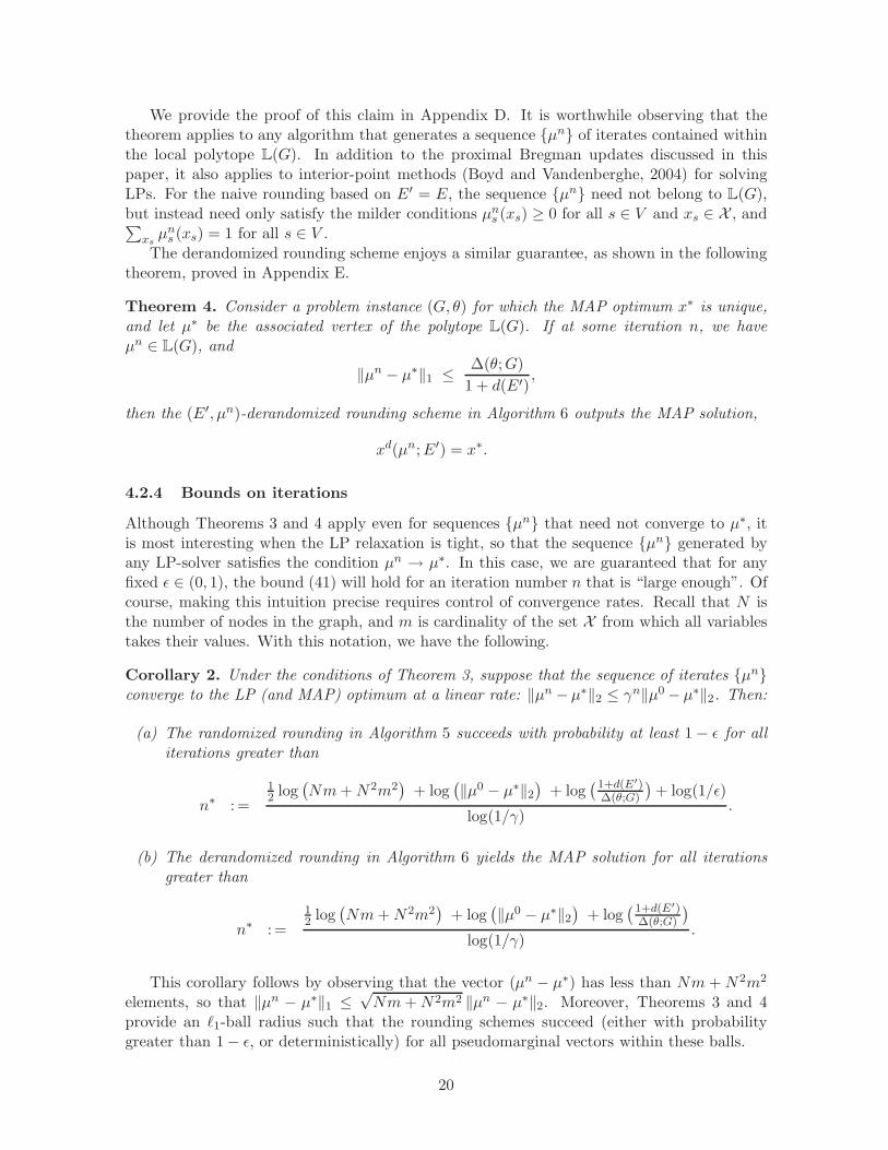
p=100p=400p=900

Figure 2. Plot of distance log10 )µn ! µ!)2 between the current entropic proximal iter-ate µn and the LP optimum µ! versus iteration number for Potts models on grids withp " {100, 400, 900} vertices, m = 5 labels and SNR = 1. Note the superlinear rate of con-vergence.

5 Experiments

We performed experiments on a 4-nearest neighbor grid graphs with sizes varying from N =100 to p = 900, using models with either m = 3 or m = 5 labels. The edge potentials were setto Potts functions, !st(xs, xt) = ,st I[xs = xt], which penalize disagreement of labels by ,st.The Potts weights on edges ,st were chosen randomly as Uniform(!1,+1), while the nodepotentials !s(xs) were set as Uniform(! SNR,SNR), where the parameter SNR & 0 controlsthe ratio of node to edge strengths, and thus corresponds roughly to a signal-to-noise ratio.

5.1 Rates of convergence

Figure 2 plots the logarithmic distance between the iterates µn of the entropic proximalmethod and the LP optimum µ", against the number of iterations for grids of di!erent sizes. Inall cases, note how the curves have an inverted quadratic shape, corresponding to superlinearconvergence. Define the suboptimality factor of an iterate as the fraction of the energy ofthe iterate to the energy of the MAP optimum. Figure 3 plots the suboptimality factor ofthe entropic proximal iterates when rounded by the node-based randomized rounding scheme,against the number of iterations. Note again, the small number of iterations required forconvergence.

5.2 Comparison of convergence rates

In Figure 4, we compare two of our proximal schemes—the entropic and the quadraticschemes—with a subgradient descent method (Feldman et al., 2002; Komodakis et al., 2007)and the max-product message passing algorithm. In particular, Komodakis et al. (2007) de-compose the LP into a sum of tractable, e.g. tree-based, objective functions by duplicatingthe parameters. They then perform (sub)gradient ascent on the dual of this decomposed LP

21

0 5 10 15 200.85

0.9

0.95

1

Iteration

Subo

ptim

ality

Rat

io

Convergence of the rounded solution

p=400p=625p=900

Figure 3. Plots of the fraction of the energy of the entropic proximal iterate µn when roundedby the node-based randomized rounding scheme to the energy of the MAP optimum µ!; versusiteration number for Potts models on grids with p " {100, 400, 900} vertices, m = 5 labels andSNR = 1. Note the small number of iterations for convergence.

0 2 4 6 8 10 12 14−600

−500

−400

−300

−200

−100

Iteration

LP E

nerg

y

LP Energy versus iteration

KomodakisEnt. Prox.Quad. Prox.Max Prod.

Figure 4. Plots comparing the convergence of the LP energy (that is, the negated LP objective)of the fractional solutions with the number of iterations for a Potts model with N = 400 vertices,m = 3 labels and SNR = 2. The methods of Komodakis et al. (2007), our entropic proximalmethod (Ent. Prox.), our quadratic proximal method (Quad. Prox.) and max product updates(Max. Prod.) are compared.

22

0 2 4 6 8 10 12 14−515

−510

−505

−500

−495

−490

−485

−480

Iteration

Roun

ded

Ener

gy

Rounded Energy versus iteration

Node Rand.Chain Rand.Node Det.Star Det.Tree Det.

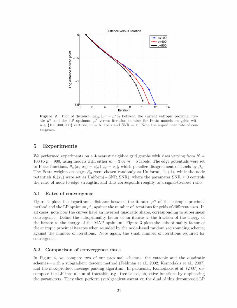
Figure 5. Plots comparing the convergence of the LP energy (that is, the negated LP ob-jective) of the rounded entropic proximal solutions with the number of iterations. The node-based (Node Rand.) and chain-based (Chain Rand.) randomized rounding schemes, and thenode-based (Node. Det.), neighborhood-based (Star Det.) and the tree-based (Tree Det.)deterministic rounding schemes are compared.

objective. For the comparison, we used a Potts model on a grid of 400 nodes, with each nodetaking 3 labels. The Potts weights were set as earlier, with SNR = 2. As Figure 4 shows, theentropic proximal scheme converges almost immediately, in six iterations, while the quadraticproximal converges quite a bit slower. The convergence rate of the subgradient ascent methodlies between those of the entropic and the quadratic proximal schemes. As the figure shows,the max-product algorithm is stuck at a fixed point away from the LP optimum.

5.3 Comparison of rounding schemes

In Figure 5, we compare five of our rounding schemes on a Potts model on grid graphs withN = 400, m = 3 labels and SNR = 2. For the graph-structured randomized rounding schemes,we used the node-based rounding scheme (so that E\E# = 0), and the chain-based roundingscheme (so that E\E# is the set of horizontal chains in the grid). For the deterministic roundingschemes, we used the node-based, neighborhood-based and the tree-based rounding schemes.As the figure shows, the node-based randomized rounding scheme converges to an almostoptimal solution almost immediately, in four iterations, closely followed by the node-basedand tree-based deterministic rounding schemes.

6 Discussion

In this paper, we have developed distributed algorithms, based on the notion of proximalsequences, for solving graph-structured linear programming (LP) relaxations. Our methodsrespect the graph structure, and so can be scaled to large problems, and they exhibit a su-perlinear rate of convergence. We have also developed a series of graph-structured roundingschemes that can be used to generate integral solutions along with a certificate of optimal-

23

ity. These optimality certificates allow the algorithm to be terminated in a finite number ofiterations.

The structure of our algorithms naturally lends itself to incorporating additional con-straints, both linear and other types of conic constraints. It would be interesting to developan adaptive version of our algorithm, which selectively incorporated new constraints as nec-essary, and then used the same proximal schemes to minimize the new conic program.

Acknowledgements

This work was partially supported by NSF grants CCF-0545862 and DMS-0528488.

A Detailed derivation of message-passing updates

In this appendix, we provided detailed derivation of the message-passing updates for the innerloops of the algorithms.

A.1 Derivation of Algorithm (2)

Consider the edge marginalization constraint for edge (s, t), Li(G) 4&

xtµst(xs, xt) = µs(xs).

Denoting the dual (Lagrange) parameter corresponding to the constraint by -st(xs), theKarush-Kuhn-Tucker conditions for the quadratic update (17) are given by

*q(µn,$+1st (xs, xt)) = *q(µn,$

st (xs, xt)) + -st(xs)

*q(µn,$+1s (xs)) = *q(µn,$

s (xs)) ! -st(xs)

µn,$+1st (xs, xt) = µn,$

st (xs, xt) + -st(xs)

µn,$+1s (xs) = µn,$

s (xs) ! -st(xs),

while the constraint itself gives

"

xt

µn,$+1st (xs, xt) = µn,$

s (xs) (43)

Solving for -st(xs) yields equation (19a). The node marginalization follows similarly, so thatoverall, we obtain message-passing Algorithm (2) for the inner loop.

A.2 Derivation of Algorithm (3)

The projection µn,$+1 = #h(µn,$ , Li(G)) onto the individual constraint Li(G) is defined bythe optimization problem:

µn,$+1 = minLi(G)

{h(µ) ! µ)*h(µn,$ )}.

Consider the subset Li(G) defined by the marginalization constraint along edge (s, t), namely&x!

t!X µst(xs, x#

t) = µs(xs) for each xs " X . Denoting the dual (Lagrange) parameters

corresponding to these constraint by -st(xs), the KKT conditions are given by

*h(µn,$+1st (xs, xt)) = *h(µn,$

st (xs, xt)) + -st(xs), and (44a)

*h(µn,$+1s (xs)) = *h(µn,$

s (xs)) ! -st(xs). (44b)

24

Computing the gradient *h and performing some algebra yields the relations

µ(n,$+1)st (xs, xt) = µ(n,$)

st (xs, xt) exp(-(n,$+1)st (xs)), (45a)

µ(n,$+1)s (xs) = µ(n,$)

s (xs) exp(!-(n,$+1)st (xs)), and (45b)

exp(2-(n,$+1)st (xs)) =

µ(n,$)s (xs)

&xt

µ(n,$)st (xs, xt)

, (45c)

from which the updates (22) follow.

Similarly, for the constraint set defined by the node marginalization constraint&xs!X µs(xs) = 1, we have *h(µ(n,$+1)

s (xs)) = *h(µ(n,$)s (xs)) + -(n,$+1)

s , from which

µ(n,$+1)s (xs) = µ(n,$)

s (xs) exp(-(n,$+1)s ), and (46a)

exp(-(n,$+1)s ) = 1/

"

xs!X

µ(n,$)s (xs). (46b)

The updates in equation (24) follow.

B Proof of Lemma 1

We provide a detailed proof for the entropic scheme; the arguments for other proximal algo-rithms are analogous. The key point is the following: regardless of how the proximal updatesare computed, they must necessary the necessary Lagrangian conditions for optimal pointsover the set L(G). Accordingly, we define the following sets of Lagrange multipliers:

-ss for the normalization constraint Css(µs) =&

x!sµs(x#

s) ! 1 = 0

-st(xs) for the marginalization constraint Cts(xs) =&

x!

tµst(xs, x#

t) ! µs(xs) = 0

'st(xs, xt) for the non-negativity constraint µst(xs, xt) & 0.

(There is no need to enforce the non-negativity constraint µs(xs) & 0 directly, since it is im-plied by the non-negativity of the joint pseudo-marginals and the marginalization constraints.)

With this notation, consider the Lagrangian associated with the entropic proximal updateat step n:

L(x;-, ') = C(µ; !, µn) + '', µ( +"

s!V

-ssCss(xs) +"

(s,t)!E

(-ts(xs)Cts(xs) + -st(xt)Cst(xt)

),

where C(µ; !, µn) is shorthand for the cost component !'!, µ( + 1(n D"(µ )µn). Using C,C #

to denote constants (whose value can change from line to line), we now take derivatives tofind the necessary Lagrangian conditions:

.L

.µs(xs)= !!s(xs) +

2%s

"nlog

µs(xs)

µns (xs)

+ C + -ss +"

t!N(s)

-ts(xs), and

.L

.µst(xs, xt)= !!st(xs, xt) +

2%st

"nlog

µst(xs, xt)

µnst(xs, xt)

+ C # + 'st(xs, xt) ! -ts(xs) ! -st(xt).

25

Solving for the optimum µ = µn+1 yields

2%s

"nlog µn+1

s (xs) = !s(xs) +2%s

"nlog µn

s (xs) !"

t!N(s)

-ts(xs) + C

2%st

"nlog µn+1

st (xs, xt) = !st(xs, xt) +2%st

"nlog µn

st(xs, xt) ! 'st(xs, xt)

+-ts(xs) + -st(xt) + C #.

From these conditions, we can compute the energy invariant (36):

2

"nF (x;µn+1) =

"

s!V

2%s

"nlog µn+1

s (xs) +"

(s,t)!E

2%st

"nlog µn+1

st (xs, xt) + C

= F (x; !) +2

"n

$ "

s!V

%s log µn(xs) +"

(s,t)!E

%st log µnst(xs, xt)

%

!"

(s,t)!E

'st(xs, xt) + C

= F (x; !) +2

"nF (x;µn) !

"

(s,t)!E

'st(xs, xt) + C.

Now since µn > 0, by complementary slackness, we must have 'st(xs, xt) = 0, which impliesthat

2

"nF (x;µn+1) = F (x; !) +

2

"nF (x;µn) + C. (47)

From this equation, it is a simple induction to show for some constants 'n > 0 and Cn " R,we have F (x;µn) = 'nF (x; !)+Cn for all iterations n = 1, 2, 3, . . ., which implies preservationof the maximizers. If at iteration n = 0, we initialize µ0 = 0 to the all-uniform distribution,then we have 2

(1 F (x;µ1) = F (x; !) + C #, so the statement follows for n = 1. Suppose that it

holds at step n; then 2(n F (x;µn) = 2

(n 'nF (x; !)+ 2Cn

(n, and hence from the induction step (47),

we have F (x;µn+1) = 'n+1F (x; !) + Cn+1, where 'n+1 = (n

2 'n.

C Proof of Theorem 2

Consider the expected cost of the configuration X(µn;E#) obtained from the randomizedrounding procedure of Algorithm 5. A simple computation shows that

E[F (X(µn;E#); !)] = G(µ̄) :=K"

i=1

H(µn;Ti) + H(µn;E#)

where

H(µn;Ti) :="

s!Vi

"

xs

µns (xs)!s(xs) +

"

(s,t)!Ei

"

xs,xt

µnst(xs, xt)!st(xs, xt), (48a)

H(µn;E#) :="

(u,v)!E!

"

xs,xt

µnu(xu)µn

v (xv)!st(xu, xv). (48b)

26

We now show by induction that the derandomized rounding scheme achieves cost at least aslarge as this expected value. Let µ̄(i) denote the updated pseudomarginals at the end of the i-thiteration. Since we initialize with µ̄(0) = µn, we have G(µ̄(0)) = E[F (X(µn;E#); !)]. Considerthe i-th step of the algorithm; the algorithm computes the portion of the derandomizedsolution xd

Viover the i!th tree. It will be convenient to use the decomposition G = Gi + G\i,

where

Gi(µ̄) :="

s!Vi

"

xs

µ̄s(xs)

$!s(xs) +

"

{t | (s,t)!E!}

"

xt

µ̄t(xt)!st(xs, xt)

%+

"

(s,t)!Ei

"

xs,xt

µ̄st(xs, xt) !st(xs, xt),

and G\i = G ! Gi. If we define

Fi(xVi) :=

"

s!Vi

!!s(xs) +

"

t: (s,t)!E!

"

xt

µ̄(i%1)t (xt)!st(xs, xt)

#+

"

(s,t)!Ei

!st(xs, xt),

it can be seen that Gi(µ̄(i%1)) = E[Fi(xVi)] where the expectation is under the tree-structured

distribution over XVigiven by

p(xVi; µ̄(i%1)(Ti)) =

7

s!Vi

µ̄(i%1)(xs)7

(s,t)!Ei

µ̄(i%1)(xs, xt)

µ̄(i%1)(xs)µ̄(i%1)(xt).

Thus when the algorithm makes the choice xdVi

= arg maxxViFi(xVi

), it holds that

Gi(µ̄(i%1)) = E[Fi(xVi

)] . Fi(xdVi

).

The updated pseudomarginals µ̄(i) at the end the i-th step of the algorithm are given by,

µ̄(i)s (xs) =

$ µ̄(i%1)s (xs) if s /" Vi

0 if s " Vi,Xd,s 2= xs

1 if s " Vi,Xd,s = xs

µ̄(i)st (xs, xt) =

$µ̄(i%1)

st (xs, xt) if (s, t) /" Ei

µ̄(i)s (xs)µ̄

(i)t (xt) if (s, t) " Ei

In other words, µ̄(i)(Ti) is the indicator vector of the maximum energy subconfiguration xdVi

.Consequently, we have

Gi(µ̄(i)) = Fi(x

dVi

) & Gi(µ̄(i%1)),

and G\i(µ̄(i)) = G\i(µ̄

(i%1)), so that at the end of the i-th step, G(µ̄(i)) & G(µ̄(i%1)). By

induction, we conclude that G(µ̄(K)) & G(µ̄(0)), where K is the total number of trees in therounding scheme.

At the end of K steps, the quantity µ̄(K) is the indicator vector for xd(µn;E#) so thatG(µ̄(K)) = F (Xd(µn;E#); !). We have also shown that G(µ̄(0)) = E[F (X(µn;E#); !)]. Combin-ing these pieces, we conclude that F (xd(µn;E#); !) & E[F (X(µn;E#); !)], thereby completingthe proof.

27

D Proof of Theorem 3

Let psucc = P[X(µn;E#) = x"], and let R(µn;E#) denote the (random) integral vertex of L(G)that is specified by the random integral solution X(µn;E#). (Since E# is some fixed forest-inducing subset, we frequently shorten this notation to R(µn).) We begin by computingthe expected cost of the random solution, where the expectation is taken over the roundingprocedure. A simple computation shows that E['!, R(µn)(] : =

&Ki=1 H(µn;Ti) + H(µn;E#),

where H(µn;Ti) and H(µn;E#) were defined previously (48).We now upper bound the di!erence '!, µ"(!E['!, R(µn)(]. For each subtree i = 1, . . . ,K,

the quantity Di : = H(µ";Ti) ! H(µn;Ti) is upper bounded as

Di ="

s!Vi

"

xs

8µ"

s(xs) ! µns (xs)

9!s(xs) +

"

(s,t)!Ei

"

xs,xt

8µ"

s(xs)µ"t (xt) ! µn

st(xs, xt)

9!st(xs, xt)

."

s!Vi

+s(!)"

xs

|µ"s(xs) ! µn

s (xs)| +"

(s,t)!Ei

+st(!)"

xs,xt

|µ"st(xs, xt) ! µn(xs, xt)|.

In asserting this inequality, we have used the fact that that the matrix with entries givenby µ"

s(xs)µ"t (xt) ! µn

st(xs, xt) is a di!erence of probability distributions, meaning that all itsentries are between !1 and 1, and their sum is zero.

Similarly, we can upper bound the di!erence D(E#) = H(µ";E#) ! H(µn;E#) associatedwith E#:

D(E#) ="

(u,v)!E!

"

xu,xv

8µ"

u(xu)µ"v(xv) ! µn

u(xu)µnv (xv)

9!uv(xu, xv)

."

(u,v)!E!

+uv(!)"

xu,xv

::::µ"u(xu)µ"

v(xv) ! µnu(xu)µn

v (xv)

::::

."

(u,v)!E!

+uv(!)"

xu,xv

$::::µ"u(xu)[µ"

v(xv) ! µnv (xv)]

::::+::::µ

nv (xv)[µ

"u(xu) ! µn

u(xu)]

::::

%

."

(u,v)!E!

+uv(!)

$"

xu

|µnu(xu) ! µ"

u(xu)| +"

xu

|µnv (xv) ! µ"

v(xv)|%

.

Combining the pieces, we obtain

'!, µ"( ! E['!, R(µn)(] . +G(!)

$)µn ! µ")1 +

"

s!V

d(s;E#)"

xs

|µns (xs) ! µ"

s(xs)|%

. (1 + d(E#))+G(!))µn ! µ")1. (49)

In the other direction, we note that when the rounding fails, then we have

'!, µ"( ! '!, R(µn)( & maxx (=x"

[F (x"; !) ! F (x; !)].

Consequently, conditioning on whether the rounding succeeds or fails, we have

'!, µ"( ! E['!, R(µn)(] & psucc('!, µ"( ! '!, µ"(

)+ (1 ! psucc) max

x (=x"

[F (x"; !) ! F (x; !)]

= (1 ! psucc) maxx (=x"

[F (x"; !) ! F (x; !)].

28

Combining this lower bound with the upper bound (49), performing some algebra, and usingthe definition of the gap $(!;G) yields that the probability of successful rounding is at least

psucc & 1 ! (1 + d(E#))

$(!;G))µn ! µ")1.

If the condition (41) holds, then this probability is at least 1 ! *, as claimed.

E Proof of Theorem 4

The proof follows that of Theorem 3 until equation (49), which gives

'!, µ"( ! E['!, R(µn)(] . (1 + d(E#)) +G(!) )µn ! µ")1.

Let vd(µn;E#) denote the integral vertex of L(G) that is specified by the derandomized integralsolution xd(µn;E#). Since E# is some fixed forest-inducing subset, we frequently shorten thisnotation to vd(µn). Theorem 2 shows that

E['!, R(µn)(] . '!, vd(µn)(.

Suppose the derandomized solution is not optimal so that vd(µn) 2= µ". Then, from thedefinition of the graph-based gap $(!;G), we obtain

'!, µ"( ! '!, vd(µn)( & +G(!)$(!;G)

Combining the pieces, we obtain

+G(!)$(!;G) . '!, µ"( ! '!, vd(µn)(. '!, µ"( ! E['!, R(µn)(]. (1 + d(E#))+G(!))µn ! µ")1,

which implies )µn ! µ")1 & !(';G)1+d(E!) . However, this conclusion is a contradiction under the

given assumption on )µn !µ")1 in the theorem. It thus holds that the derandomized solutionvd(µn) is equal to the MAP optimum µ", thereby completing the proof.

References

M. Bayati, D. Shah, and M. Sharma. Maximum weight matching for max-product beliefpropagation. In Int. Symp. Info. Theory, Adelaide, Australia, September 2005.

M. Bayati, C. Borgs, J. Chayes, and R. Zecchina. Belief-propagation for weighted b-matchingson arbitrary graphs and its relation to linear programs with integer solutions. TechnicalReport arxiv:0709.1190, Microsoft Research, September 2007.

U. Bertele and F. Brioschi. Nonserial dynamic programming. Academic Press, New York,1972.

D. P. Bertsekas and J. N. Tsitsiklis. Parallel and Distributed Computation: Numerical Meth-ods. Athena Scientific, Boston, MA, 1997.

29

D.P. Bertsekas. Nonlinear programming. Athena Scientific, Belmont, MA, 1995.

D. Bertsimas and J. Tsitsikilis. Introduction to linear optimization. Athena Scientific, Bel-mont, MA, 1997.

J. Besag. On the statistical analysis of dirty pictures. Journal of the Royal Statistical Society,Series B, 48(3):259–279, 1986.

S. Boyd and L. Vandenberghe. Convex optimization. Cambridge University Press, Cambridge,UK, 2004.

Y. Boykov, O. Veksler, and R .Zabih. Fast approximate energy minimization via graph cuts.IEEE Trans. Pattern Anal. Mach. Intell., 23(11):1222–1239, 2001.

Y. Censor and S. A. Zenios. Parallel Optimization - Theory, Algorithms and Applications.Oxford University Press, 1997.

C. Chekuri, S. Khanna, J. Naor, and L. Zosin. A linear programming formulation and approxi-mation algorithms for the metric labeling problem. SIAM Journal on Discrete Mathematics,18(3):608–625, 2005.

F. Deutsch and H. Hundal. The rate of convergence for the cyclic projection algorithm I:Angles between convex sets. Journal of Approximation Theory, 142:36 55, 2006.

J. Feldman, D. R. Karger, and M. J. Wainwright. Linear programming-based decoding ofturbo-like codes and its relation to iterative approaches. In Proc. 40th Annual AllertonConf. on Communication, Control, and Computing, October 2002.

W. T. Freeman and Y. Weiss. On the optimality of solutions of the max-product beliefpropagation algorithm in arbitrary graphs. IEEE Trans. Info. Theory, 47:736–744, 2001.

S. Geman and D. Geman. Stochastic relaxation, Gibbs distributions, and the Bayesian restora-tion of images. IEEE Trans. PAMI, 6:721–741, 1984.

A. Globerson and T. Jaakkola. Fixing max-product: Convergent message passing algorithmsfor MAP LP-relaxations. In Neural Information Processing Systems, Vancouver, Canada,December 2007.

D.M. Greig, B.T. Porteous, and A.H. Seheult. Exact maximum a posteriori estimation forbinary images. Journal of the Royal Statistical Society, Series B, 51, 1989.

T. Hazan and A. Shashua. Convergent message-passing algorithms for inference over gen-eral graphs with convex free energy. In The 24th Conference on Uncertainty in ArtificialIntelligence (UAI), Helsinki, 2008.

B. Huang and T. Jebara. Loopy belief propagation for bipartite maximum weight b-matching.In AISTATS, San Juan, Puerto Rico, March 2007.

A. N. Iusem and M. Teboulle. Convergence rate analysis of nonquadratic proximal methodsfor convex and linear programming. Mathematics of Operations Research, 20(3):657–677,1995.

30

J. K. Johnson, D. M. Malioutov, and A. S. Willsky. Lagrangian relaxation for MAP estimationin graphical models. In Proc. 45th Allerton Conf. Comm. Cont. Comp., Urbana-Champaign,IL, September 2007.

J. Kleinberg and E. Tardos. Approximation algorithms for classification problems with pair-wise relationships: Metric labeling and Markov random fields. In IEEE Symp. Found.Comp. Science, pages 14–24, 1999.

V. Kolmogorov. Convergent tree-reweighted message-passing for energy minimization. InInternational Workshop on Artificial Intelligence and Statistics, January 2005.

V. Kolmogorov and M. J. Wainwright. On optimality properties of tree-reweighted message-passing. In Uncertainty in Artificial Intelligence, July 2005.

N. Komodakis, N. Paragios, and G. Tziritas. MRF optimization via dual decomposition:Message-passing revisited. In ICCV, Rio di Janeiro, Brazil, 2007.

V. K. Koval and M. I. Schlesinger. Two-dimensional programming in image analysis problems.USSR Academy of Science, Automatics and Telemechanics, 8:149–168, 1976. In Russian.

P. Kumar, P.H.S. Torr, and A. Zisserman. Solving markov random fields using second ordercone programming. IEEE Conference of Computer Vision and Pattern Recognition, 2006.

S. L. Lauritzen. Graphical Models. Oxford University Press, 1996.

P. Raghavan and C. D. Thompson. Randomized rounding: A technique for provably goodalgorithms and algorithmic proofs. Combinatorica, 7(4):365–374, 1987.

P. Ravikumar and J. La!erty. Quadratic programming relaxations for metric labeling andmarkov random field map estimation. In ICML ’06: Proceedings of the 23rd internationalconference on Machine learning, pages 737–744, 2006.

S. Sanghavi, D. Shah, and A. Willsky. Message-passing for max-weight independent set. InNeural Information Processing Systems, Vancouver, Canada, December 2007.

M.V. Solodov and B.F. Svaiter. A unified framework for some inexact proximal point algo-rithms. Numerical Functional Analysis and Optimization, 22:1013–1035, 2001.

P. Tseng and D. P. Bertsekas. On the convergence of the exponential multiplier method forconvex programming. Math. Programming, 60:1—19, 1993.

M. J. Wainwright and M. I. Jordan. Graphical models, exponential families, and variationalinference. Technical report, UC Berkeley, Department of Statistics, No. 649, September2003.

M. J. Wainwright and M. I. Jordan. Treewidth-based conditions for exactness of the Sherali-Adams and Lasserre relaxations. Technical report, UC Berkeley, Department of Statistics,No. 671, September 2004.

M. J. Wainwright, T. S. Jaakkola, and A. S. Willsky. Tree-based reparameterization frameworkfor analysis of sum-product and related algorithms. IEEE Trans. Info. Theory, 49(5):1120–1146, May 2003.

31

M. J. Wainwright, T. S. Jaakkola, and A. S. Willsky. Tree consistency and bounds on themax-product algorithm and its generalizations. Statistics and Computing, 14:143–166, April2004.

M. J. Wainwright, T. S. Jaakkola, and A. S. Willsky. Exact MAP estimates via agreement on(hyper)trees: Linear programming and message-passing. IEEE Trans. Information Theory,51(11):3697–3717, November 2005.

Y. Weiss, C. Yanover, and T. Meltzer. Map estimation, linear programming and belief prop-agation with convex free energies. In Uncertainty in Artificial Intelligence, 2007.

C. Yanover, T. Meltzer, and Y. Weiss. Linear programming relaxations and belief propagation:An empirical study. Journal of Machine Learning Research, 7:1887–1907, September 2006.

J.S. Yedidia, W. T. Freeman, and Y. Weiss. Constructing free energy approximations andgeneralized belief propagation algorithms. IEEE Trans. Info. Theory, 51(7):2282–2312, July2005.

32