Journal of Colloid and Interface Science 247, 463–480 (2002)doi:10.1006/jcis.2001.8109, available online at http://www.idealibrary.com on

Mesoscopic Dispersion of Colloidal Agglomerate in a ComplexFluid Modelled by a Hybrid Fluid–Particle Model

Witold Dzwinel∗,1 and David A. Yuen†∗AGH Institute of Computer Science, Al.Mickiewicza 30, 30-059 Krakow, Poland; and †Minnesota Supercomputer Institute,

University of Minnesota, Minneapolis, Minnesota 55415-1227

E-mail: dzwinel@uci.agh.edu.pl; davey@krissy.msi.umn.edu

Received March 27, 2001; accepted November 24, 2001

The dispersion of the agglomerating fluid process involving col-loids has been investigated at the mesoscale level by a discrete par-ticle approach—the hybrid fluid–particle model (FPM). Dynamicalprocesses occurring in the granulation of colloidal agglomerate insolvents are severely influenced by coupling between the dispersedmicrostructures and the global flow. On the mesoscale this couplingis further exacerbated by thermal fluctuations, particle–particle in-teractions between colloidal beds, and hydrodynamic interactionsbetween colloidal beds and the solvent. Using the method of FPM,we have tackled the problem of dispersion of a colloidal slab beingaccelerated in a long box filled with a fluid. Our results show thatthe average size of the agglomerated fragments decreases with in-creasing shearing rate �, according to the power law A · �k, wherek is around 2. For larger values of �, the mean size of the agglom-erate Savg increases slowly with � from the collisions between theaggregates and the longitudinal stretching induced by the flow. Theproportionality constant A increases exponentially with the scalingfactor of the attractive forces acting between the colloidal particles.The value of A shows a rather weak dependence on the solvent vis-cosity. But A increases proportionally with the scaling factor of thecolloid–solvent dissipative interactions. Similar type of dependencecan be found for the mixing induced by Rayleigh–Taylor instabili-ties involving the colloidal agglomerate and the solvent. Three typesof fragmentation structures can be identified, which are called rup-ture, erosion, and shatter. They generate very complex structureswith multiresolution character. The aggregation of colloidal beds isformed by the collisions between aggregates, which are influencedby the flow or by the cohesive forces for small dispersion energies.These results may be applied to enhance our understanding con-cerning the nonlinear complex interaction occurring in mesoscopicflows such as blood flow in small vessels. C© 2002 Elsevier Science (USA)

Key Words: hybrid fluid–particle model; mesoscopic flow; col-loidal agglomerates; fragmentation; agglomeration.

1. INTRODUCTION

Mesocopic flows are important to understand because theyhold the key to the interaction between the macroscopic flow

1 To whom correspondence should be addressed.

463

and the microstructures. This is especially true in colloidalflows, which involve colloidal mixtures, thermal fluctuations,and particle–particle interactions. In many technological andphysical processes, such as emulsification, formation of nanojets(1), water desalination, food production, gel filtration, and trans-port processes in sedimentary rocks (2) or in tiny blood vessels,the microscopic or microstructural effects may even dominateover the hydrodynamical processes and these phenomena takeplace in the realm of mesoscopic flows. For example, blood is asystem rich in rheological properties, exhibiting shear-thinning,viscoelastic, and sedimenting behavior. But still, only qualita-tive correlations have ever been made between the observed mi-crostructure and the reported rheology. Central to understandingthese correlations is the determination of the intrinsic link be-tween the rheology and the microstructure.

There exists a large body of knowledge on theoretical, ex-perimental, and numerical models of various aspects of flow ofpowdered solids in liquid (3). However, colloidal beds cannotbe treated as dry powders. In a general sense, colloids com-prise two types of particles, large and small ions, which aresuspended in a solvent. Colloidal agglomerates consist of largeions due to complex ion–ion and ion–solvent interactions, whichare of entropic and electrostatic origin (4). The classical modelsof powder granulation in liquids assume that the Peclet numberis much greater than unity and the agglomerate size is muchlarger than the interaction range of cohesion forces (3). Thismeans that thermal fluctuations, diffusion effects in liquid, andmicroscopic interactions are neglected. For these assumptionsfragmentation microstructures such as rupture, erosion, shat-ter, and aggregation processes can be considered separately. Inthe mesoscale, with the presence of diffusion, thermal fluctu-ations, and long-range interactions between colloidal particles,fragmentation and aggregation microstructures usually occur si-multaneously or overlap.

Since blood can be regarded as a colloid (5), we will use it asan example to explain the rationale of our modeling. The axisym-metric pulsatile flows and flows subject to acceleration in bloodvessels have been investigated both experimentally and numer-ically for a long time (see, e.g., (6–9)). These investigations

0021-9797/02 $35.00C© 2002 Elsevier Science (USA)

All rights reserved.

A

464 DZWINEL

were focused on the influence of material damping on the wallvessels, of the viscoelastic properties (10) of blood on the flow of,deformation properties of blood vessels from the shear stressesexerted on the wall, and of the mass transfer and fluid dynam-ics of blood flow. All of these phenomena can be simulatedusing Navier–Stokes equations with proper substitution of theblood rheological properties. However, there are medical cir-cumstances in which the Navier–Stokes equations with simplerheology may not work: rapid heart attack or a rapid stroke de-veloped by sudden clotting in small blood vessels. These are crit-ical phenomena in which a transition has taken place in the mi-croscale and propagates over to the mesoscale and macroscale.In this mesoscale regime, blood’s rheology has changed and itshould be treated as a complex fluid with various kinds of mi-crostructures, which have suddenly been developed. A reviewof the relevant concepts in block of microcirculation in bloodvessels was first given by Fung and Zwiefach (11). Until nownot much progress has been made in the field in these aspectsconcerning the flow interactions between the microstructural dy-namics and the larger-scale flow. The modeling of the dispersionof drugs and thrombus along tiny blood vessels needs a com-pletely different approach, which is still undetermined. In thispaper we will model the colloidal interactions between these re-

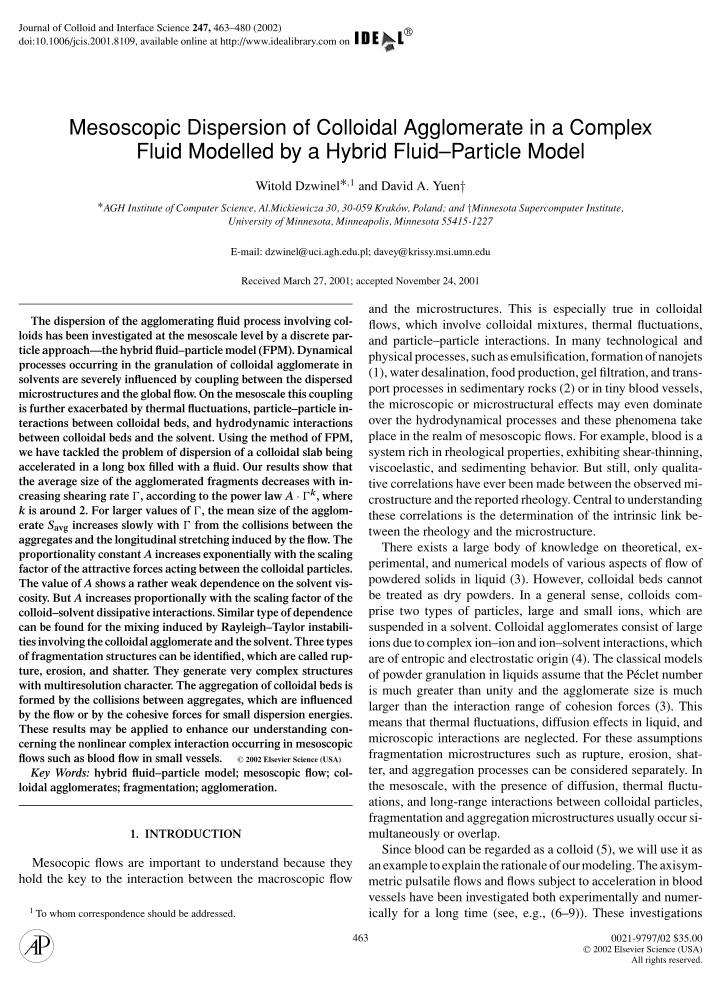
cently formed microstructures with the complex types of flows molecular dynamics (MD) forms the centerpiece from which the by means of a discrete particle model. other techniques, such as dissipative particle dynamics (DPD)

FIG. 1. The principal differences between selected discrete particle models: digas (LBG), stochastic rotational dynamics (RSD), and molecular dynamics (MD)

ND YUEN

Microscopic techniques employing discrete particles such asmolecular dynamics (MD) and Monte Carlo (MC) are very use-ful in studying interactions between primary particles, whichform molecules and microstructures. For example, the large-scale MD simulations were employed for investigating micro-scopic flows (1, 12, 13) and microstructures in solid materialssuch as impurities in crystals and cracks (14). However, MD be-comes too demanding for simulating larger particle ensembles.At the present time particle systems of size about 1 µm can besimulated by using 109 atoms over tens of nanoseconds on thelargest parallel computers (14). Most of the computations spendtime producing information on microscopic fluctuations, whichare not necessary for scales in the ordering of complex fluids.

In recent years, new numerical methods have been devel-oped for modeling physical and chemical phenomena occurringin the mesoscale. The most popular are lattice Boltzmann gas(LBG) (15–17), diffusion-limited aggregation (18), direct nu-merical simulations (DNS) (19, 20), or other particle methodssuch as stochastic rotational dynamics (SRD) (21), fluid parti-cle dynamics (FPD) (22), dissipative particle dynamics (DPD)(23), and fluid particle model (FPM) (24). In Fig. 1 we depict theprincipal features of some of discrete particle models employedfor simulation of complex fluids in the mesoscale. We note that

ssipative particle dynamics (DPD), fluid particle model (FPM), lattice Boltzmann.

1 1

DISPERSION OF COLLOIDAL AGG

and fluid particle model ( FPM), are derived and are applicableover a longer length scale.

Dissipative particle dynamics (DPD) is one of the mesoscopictechniques, which allows one to model hydrodynamic behav-ior with thermal fluctuations. This particle-based off-lattice al-gorithm was inspired by ideas coupling the advantages of themolecular dynamics and lattice-gas methods. A strong back-ground drawn from statistical mechanics has been provided toDPD (25) from which explicit formulas for transport coefficientsin terms of the particle interactions can be derived. Since thenthe DPD model has attracted a great deal of attention from thechemical community (see, e.g., (26–28)).

As shown in (29, 30), DPD can be used for studying varioustypes of phase separation processes in binary or multicomponentfluids. By employing two-level models for which colloidal bedsare modeled by MD particles and solvent by DPD fluid parti-cles, one can simulate micellar solutions (31) and large colloidalaggregates, which can use as many as 20 million particles (32).Dissipative particle dynamics can also be employed for simulat-ing hydrodynamical instabilities such as thin-film falling downthe inclined plane (33), the breakup of droplets and mixing incomplex fluids (26, 34–36).

For simulating mixing of colloidal agglomerates, over themesoscale, we have implemented generalized version of dissi-pative particle dynamics DPD devised by Espanol (24)—thefluid–particle model (FPM)—which is hybridized within theframework of a classical MD code. We first describe the model.We then present the results from the FPM simulations. Finallywe summarize our findings and discuss the prospects of em-ploying the discrete particle method in modeling dynamics ofcomplex colloidal fluid in the mesoscale.

2. DESCRIPTION OF THE FLUID PARTICLE MODEL (FPM)

We begin our discussion by first going over some rudimentsof the dissipative particle dynamics (DPD) method (23). TheDPD technique portrays the mesoscopic portions of a real fluid.They can be viewed as “droplets” of liquid molecules with aninternal structure and with some internal degrees of freedom.As shown in (24, 25), the interactions between these parti-cles are postulated from simplicity and symmetry principles.These principles ensure their correct hydrodynamic behavior.The advantage of DPD over other methods, such as lattice-gasor lattice-Boltzmann, lies in the possibility of matching the scaleof discrete-particle simulation to the dominant spatiotemporalscales of the entire system (24).

One of the serious drawbacks of DPD is the absence of a dragforce between the central particle and the second particle orbit-ing about the first. This relative motion may produce a net drag,when many DPD particles are participating at the same time(24). This cumulative effect would reduce the computational ef-ficiency of the DPD method. For this reason, the fluid–particlemethod (FPM) has been introduced by means of a noncentral

force, which is proportional to the difference between the ve-locities of the particles (24). This will eliminate this deleterious

LOMERATE IN COMPLEX FLUID 465

effect from the net drag force. Additionally, this FPM approachwould allow the simulation of physical effects associated withrotational diffusion and rotation of the colloidal beds resultingfrom hydrodynamic or their mutual interactions.

The theoretical framework for the FPM was presented byEspanol (24). We retain here the original notation used in (24).The fluid particles possess several attributes such as mass, mi ,position, ri , translational and angular velocities, and type. The“droplets” interact with each other by forces dependent on thetype of particles. We use the two-body, short-ranged force Fas it is postulated in (24). This type of interaction is a sumof a conservative component FC, two dissipative componentsFT and FR, and a Brownian force F; that is,

Fi j = FCi j + FT

i j + FRi j + Fi j . [1]

The FPM force components are defined by

FCi j = −V ′(ri j ) · ei j [2]

FTi j = −γ mTi j · vi j [3]

FRi j = −γ mTi j ·

(1

2ri j × (ωi + ω j )

)[4]

Fi j dt = (2kBT γ m)1/2

(A(ri j ) dWS

i j + B(ri j )1

Dtr [dW]1

+ C(ri j ) dWAi j

)· ei j , [5]

where ri j is a distance between particles i and j , ri j = ri − r j is avector pointing from particle i to particle j and ei j = ri j/ri j , D isthe dimensionality of the model, T0 is the temperature of particlesystem, kB is the Boltzmann constant, dt is the time step, γ isa scaling factor for dissipation forces, ω is the angular velocity,dWS, dWA, tr[dW]1 are symmetric, antisymmeric, and tracediagonal random matrices of independent Wiener incrementsdefined in (24), and A(r ), B(r ), C(r ), A(r ), B(r ), C(r ), V ′(r )are functions dependent on the separation distance r = ri j .

Ti j is a dimensionless matrix given by

Ti j = A(ri j )1 + B(ri j )ei j ei j . [6]

1 is the unit matrix.As was shown in (24), the single-component FPM system

yields the Gibbs distribution as the steady-state solution to theFokker–Planck equation under the condition of detailed bal-ance. Consequently it obeys the fluctuation–dissipation theorem,which defines the relationship between the normalized weightfunctions, which are chosen so that

A(r ) = 1

2[ A2(r ) + C2(r )],

[7]

B(r ) =D

[B2(r ) − A2(r )] +2

[ A2(r ) − C2(r )].

466 DZWINEL A

For the dissipative particle dynamics (DPD) method A(r ) = 0;consequently A(r ), B(r ) = 0, and V ′(r ) ∝ B(r ), which meansthat all the DPD forces are central.

The noncentral force in FPM, which is proportional to thedifference between particle velocities, introduces an additionaldrag lacking in the DPD model. The noncentral force resultsalso in additional rotational friction given by Eq. [4].

The temporal evolution of the particle ensemble obeys theNewtonian laws of motion,

vi = 1

m

∑j �=i

Fi j [8]

ri = vi [9]

ωi = 1

I

∑j �=i

Ni j , [10]

where the torques in Eq. [11] are given by

Ni j = −1

2ri j × Fi j . [11]

The FPM can predict precisely the transport properties ofthe fluid, thus allowing one to adjust the model parametersaccording to the formulas of kinetic theory. Unlike in themacroscopic particle-based method—smoothed particle dynam-ics SPH (37)—the angular momentum is conserved exactly inFPM. In short, the FPM model can be physically interpreted asa Lagrangian discretization of the nonlinear fluctuating hydro-dynamic equations.

3. NUMERICAL MODEL

We have employed a two-dimensional model of a simula-tion clearly involving a three-dimensional process. However,the simplified 2-D models are less time-consuming than 3-Dmodels and we can certainly glean some useful basic informa-tion before venturing into the 3-D arena. It is a matter of morecomputer time to carry out 3-D simulations with the FPM.

This is a two-level approach and we will consider two typesof particles: solvent droplets and colloidal beds. We assumethat the concentration of electrolyte in the solvent is low, whichis appropriate for the blood. In this case we can neglect thelong-range interactions and focus just on the short-range forces.Therefore, the electrolyte-solvent particles can be representedby FPM fluid particles.

We assume that the weight functions (Eqs. [6], [7]) satisfy theconditions imposed. Due to the degree of freedom allowed bythe model in selecting the weight functions we may assume that

A(r ) = 0, A(r ) = B(r ) =(

1 − r

rcut

)2

,

[12]′ 3

(r

)

V (r ) = −

πr2cutn

1 −rcut

,

ND YUEN

where rcut is a cut-off radius, which defines the range of particle–particle interactions. For ri j > rcut, Fi j = 0. The first assump-tion is recommended in (24). We postulate the rest of the weightfunctions the same as in DPD (22, 24). Due to additional drag be-tween particles caused by the noncentral interactions we can re-duce the computational load assuming that the interaction rangeis shorter than for DPD fluid.

The colloidal agglomerates consist of primary particles—thecolloidal beds. They can represent large charged ions, whichare a few times larger than electrolyte-solvent droplets. We as-sume that the agglomerates are “wet”; i.e., colloidal beds arecovered by electrolyte binder. This assumption allows us to usein the model mean forces similar to those obtained for chargedmacroions in realistic colloidal mixtures.

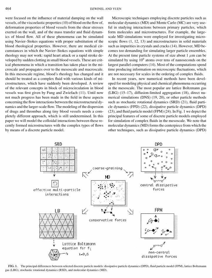
Interactions among colloidal particles have been studied formore than 50 years. Colloids can be regarded as a complexmany-body systems described by highly approximate treatmentsdrawn from classical statistical physics. As follows from the con-ventional Derjaguin–Landau–Verwey–Overbeek (DLVO) the-ory the long-range electrostatic interaction between colloidalspheres can be modeled by a screened Coulomb repulsion (38).Additional interactions come from hydrodynamic (39) and de-pletion forces (40). Some experimental findings (39, 41) showthat like-charged macroions have been attracted to one anotherby short-ranged forces. This fact cannot be explained by theconventional theories. The recent simulation results (4) showthat the fluctuation of the charge distribution by the small ionsresults in the attraction between microions. The mean force isa combination of hard-sphere and electrostatic force. As an ap-proximation V ′(ri j ) (see Eq. [2]) of the mean force between col-loidal beds, we use the sum of the Lennard–Jones (L–J) forceand a very steep force with a soft core. In Fig. 2 we depictthat the approximation is very close to the mean force obtainedfrom large-scale Monte Carlo calculations performed for a realcolloidal mixture (4). The force well is proportional to ε—theminimum L–J potential—which is called here the cohesion fac-tor. Unlike in our previous papers exploiting the two-level model(31, 32, 35), we introduce additional dissipative force betweencolloidal beds. This force is responsible for dissipation of en-ergy due to bed collisions. The colloidal particles are largerand heavier than FPM “droplets” and their interactions are sin-gular. Therefore, thermal fluctuations are transferred from thebulk of fluid and are partly dissipated inside the colloidal ag-glomerates (Fi j = 0, if i and j are colloidal particles). There isalso no central drag between colloidal beds (B(ri j ) = 0) becausethe binder layer covering colloidal beds is assumed to be verythin.

The bed–“droplet” interactions are simulated by employingFPM forces. This is justifiable on the following grounds:

1. The bed–“droplet” forces cannot be singular.2. Nonzero Brownian component (Fi j �= 0) comes from the

fluid “droplet.”

3. Viscous drag (B(ri j ) �= 0) comes from the fluid “droplet”

and the electrolyte binder.

DISPERSION OF COLLOIDAL AGG

FIG. 2. The mean force between colloidal particles as a function of macroionseparation (in units of macroion diameter) approximated by the sum of the L-Jforce and soft sphere repulsion. Black dots show the approximate shape of themean force obtained from Monte Carlo simulation of a macroion’s interactionsin a real colloidal mixture (4).

4. The electrolyte concentration in electrolyte–solvent mix-ture surrounding the agglomerate is low, thus electrostatic bed–“droplet” interactions are negligibly small.

Because the colloidal bed contains a hard core, we have mod-ified the repulsive part of the conservative FC bed–“droplet”forces, thus making it steeper than for “droplet”–“droplet” in-teractions.

The FPM model is based on concepts drawn from statisticalphysics. In contrast to DPD and two-level models used in our ear-lier simulations, it is a more general and self-consistent particlemethod. Simulation of multiphase flow consists of appropriatedefinition of conservative forces between particles representingdifferent phases and setting some interactions to zero. Thermo-dynamic properties of the model and the detailed balance condi-tions are always preserved according to the rigorous theoreticalbasis set out in (24).

The forces are computed by using O(M) order (M-number ofparticles) link-list scheme combined with neighbor tables (42).Multiple link-lists are used because the sizes of particles andranges of interactions (rcut) are different; that is, larger Hockneycells (42) are used for longer-ranged interactions.

In the integration of the equations of motion, which are, infact, stochastic differential equations (SDE), we have employedat first the leap-frog numerical scheme as it is in (23, 29). Becausethe scheme is only an approximation of stochastic integrator it

generates artifacts leading to unphysical correlations and mono-tonically increasing (or decreasing) temperature drift. Due to

LOMERATE IN COMPLEX FLUID 467

large instabilities observed by using leap-frog, we have used thefollowing higher-order temporal O( t4) scheme for ω,

ωn+1/2i = 2ω

n−1/2i − ω

n−2/3i + (

Nni − Nn−1

i

), [13]

while the values of vn+1 and ωn+1 are predicted by using theO( t2) Adams–Bashforth procedure as in (30). As shown in(35), both the hydrodynamic temperature and hydrodynamicpressures do not exhibit noticeable drift for 1 million time steps.However, the hydrodynamic temperature is 2% higher than theassumed temperature. This is due to the non-energy-conservingcharacter of the scheme applied. However, the detailed balancecondition appeared to be only slightly violated (35). For simula-tions requiring more accurate conservation of thermodynamicalquantities, another integrator, which uses a thermostat, shouldbe considered.

The parameters associated with the fluid dynamical interac-tions of FPM have been matched to the fluid transport coeffi-cients by using the equations in the continuum limit and thedetailed balance condition (24),

Pk �=l = nk �=l〈r〉2D

[14]

νb = γ n

[A2

2D+ D + 2

2DB2

]+ c2 1

γ Dn(A0 + B0)[15a]

νS = 1

2γ n

[A2

2+ B2

]+ c2 1

2γ n(A0 + B0)[15b]

νR = γ n A2

2[15c]

A0 =∫

drA(r ), B0 = 1

D

∫drB(r ),

[16]

A2 = 1

D

∫drr2 A(r ), B2 = 1

D(D + 2)

∫drr2 B(r )

γ = σ 2m

2kBT, [17]

where P is a partial pressure, T0 is the temperature of the particlesystem, νb, νS, νR are bulk, shear, and rotational kinematic vis-cosities, respectively, and D = 2, c2 = kBT/m, and , σ , andγ are scaling factors of conservative, Brownian, and dissipativeforces, respectively.

The results of our test runs show that our FPM model satisfiesthe basic physical constraints:

1. Total angular and translational momenta are preserved.2. The actual thermodynamical pressure computed from the

virial theorem is constant. Its average is 5–10% larger than Passumed (for M = 50,000 particles).

3. The actual thermodynamical temperature computed from

the average kinetic energy of the particle system is constant anddeviates no more than 2–5% from the value of T .

468 DZWINEL A

4. The rotational kinetic energy is about one-third of the totalkinetic energy.

Since the compressibility of the fluid is low (for a large valueof ), there are some quantitative differences between the theoryand the simulation. The kinetic theory formulas have been devel-oped in the limit where no conservative forces are present. Theactual transport coefficients computed from generalized Einsteinand Green–Kubo formulas (43) are larger more than 50% thanthose predicted from the classical kinetic theory (44). Therefore,the transport coefficients computed from the theory can be usedonly as the first coarse approximation. The most precise match-ing can be done by using a new generic formulation of DPDmodel, which is a natural generalization of both the DPD andFPM (47).

We have solved the problem for finding clusters of very so-phisticated shapes created during granulation by employing anefficient O(M) clustering procedure. It is based on the mutualnearest neighboring (mnn) distance concept. This procedure isoutlined in (32).

In Table 1 we have collected dimensionless units used in themodel. To define the transport properties of liquid, we introducedimensionless dissipation factor � as it is in (45),

� = γ rc/Dc, [18]

where D is the dimensionality of the system. For the two-phasesolvent–colloid system we have defined three � values: �1–1 forcolloid-colloid, �1–2 for colloid-solvent, and �2–2 for solvent–solvent interactions. The value of �2–2 represents the magnitudeof the viscous forces in the solvent assuming that the conserva-tive forces between fluid particles are small or negligible. Forthe colloidal system, the value of �1–1 characterizes only the

dissipative component of colloid–colloid interactions. Becausethe viscous forces depend also on the long-range correlations

ders of magnitude larger than a molecule, which would put itaround 0.1 to 1 µm. The problems with simulating an ensemble

TABLE 2Principal Physical and Numerical Parameters

General parameters Values

T 1g 0.00001 λ/ t2

t 0.008

Types of interactions → Liquid particle–liquid particle Liquid particle–colloidal bed Colloidal bed–colloidal bed

Average distance between neighboring particles λ 1 1.5 1.5Number density 3.2 (particles in sphere of radius λ) 3.2 3.2Cut-off radius (in λ) 1.5 2.5 1.8Particle mass m1 = 1 m1,2 = 2m1m2/(m1 + m2) m2 = 22.5

Sound velocity√

Pρ

(in c) 7.4 — 1.5

Dissipation factor � 25 25 10Cohesion factor ε — — 0–4Number of particles 1 × 105 — 2 × 103

(for large-scale R-T simulations) (1 × 106)

ND YUEN

TABLE 1Program Units

Value Unit

Length λ The average distance between theneighboring fluid particles

Mass m Dimensionless, mass of the lightestfluid particle m = 1

Time t In t = λ/c where c2 = kBT/m; λ,unit of length

Energy εunit In 3kBT (average kinetic energy forMaxwell distribution)

Dissipation factor � � = γ rc/2c where γ is the scalingfactor of dissipative forces

resulting from conservative interactions between colloidal beds,the shear viscosity in the colloidal system cannot be computeddirectly from Eq. [15b]. The actual transport coefficients canbe obtained from the Green–Kubo formula employing averagedautocorrelation functions from direct simulation. For the sake ofsimplicity we use instead of viscosity the dissipative factors �

representing the magnitude of the viscous forces resulting fromonly dissipative component of interparticle forces. The scalingfactor for dissipative component of DPD force, defined by thedimensionless � parameter, is set between 10 and 100 (45). For� value greater than 100 the integration scheme becomes numer-ically unstable but � = 10–90 yields reasonably fast relaxationfor medium temperatures corresponding to the [1–4] interval inεunit units (see Table 1).

Table 2 comprises the principal dimensionless parametersused in 2D simulations. Since the droplets represent clustersof molecules, we can estimate that a colloidal bed is a few or-

— (5 × 104)

469

We study two taccelerated in a p

DISPERSION OF COLLOIDAL AGGLOMERATE IN COMPLEX FLUID

a

FIG. 3. Velocity profiles with simulation time. The V-sh

consisting of particles with such different sizes result from thedifferent time scales in which the both types of particles evolve.By approximating the solvent using FPM particles of size similarto that of the colloidal particles, we have met the requirementsof both scales. The mass variation can be simulated by usingdifferent masses of solvent and colloid particles and/or differentparticle sizes for the solvent and colloid. We assume that

1. spacing between colloidal beds is 50% greater than forliquid “droplets” (thus the colloidal beds are bigger);

2. the density of the colloidal system is 10 times greater thanthe density of the liquid (for such a contrast in density and differ-ence in size of particles, the mass of a colloidal particle should bemore than 20 times greater than the mass of a solvent particle).

The value of —the scaling factor for conservative FPM forces,which is responsible for the compressibility of the fluid (repre-sented by the velocity of sound in Table 2)—is chosen so thatthe particle system exhibits liquid ordering in the mesocale; i.e.,its RDF (the radial distribution function) is characteristic of theliquid phase. As it is suggested in (30), the value of wascomputed assuming that the FPM fluid has the compressibilitycharacteristic of water. The energy unit (εunit) is set arbitrarilyas a reference point for scaling the colloid–colloid interactions.It is measured in 3kBT (average kinetic energy for Maxwell dis-tribution) dimensionless units. The cohesion factor is given inεunit and is equal to the ε parameter of the Lennard–Jones force.

The existence of the noncentral force in the FPM allows foremploying a shorter cut-off radius for forces calculation than inDPD simulations, thus saving computational time. A typical cut-off radius used in DPD simulation is 2.5λ (23, 29). The numberdensity from Table 2 is also representative for MD and DPDsimulations of liquids in 2D.

The system size depends on the total number of particles M .Due to the multiresolution patterns created during flow we usemedium-sized particle ensembles ranging from 105 to 106 par-ticles simulated for 104–105 time steps.

ypes of flow. At first we consider a colloidal slaberiodic box. Similar types of flows were studied

ped profile becomes stable after about 15,000 time steps.

for solid–liquid mixing by assuming a constant shear rate (3).By using an accelerated flow we can investigate the granulationof colloidal agglomerate over a broad range of kinetic energiesin the flow with a single simulation. The particles are confinedwithin the rectangular box with periodic boundary conditionsin y and reflecting walls in x direction. The aspect ratios of theslab to the box dimensions are 1 : 5 and 1 : 10 along the x and yaxes, respectively. As shown in Fig. 3, the V-shaped profile ofvelocity field stabilizes after about 15,000 time steps. Over thewhole periodic box along both the x and y directions we canobserve strong correlations along the horizontal direction. Thevertical correlations are weaker due to greater aspect ratio andvanishing velocity gradients in the y direction. In the followingsection we report the simulation results of granulation for thistype of flow.

4. DISPERSION OF COLLOIDAL SLAB IN A PERIODIC BOX

In Figs. 4 and 5 we present the snapshots from 2-D FPMsimulations of dispersion of colloidal agglomerate acceleratedin a periodic box. We recognize several stages of granulation,which usually occur with some degree of overlap:

FIG. 4. Imbibition of colloidal agglomerate by fluid particles for differentcohesion factor ε.

470 DZWINEL A

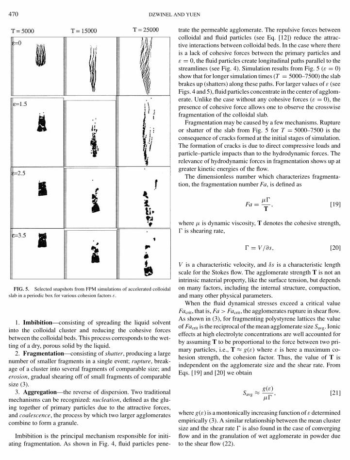
FIG. 5. Selected snapshots from FPM simulations of accelerated colloidalslab in a periodic box for various cohesion factors ε.

1. Imbibition—consisting of spreading the liquid solventinto the colloidal cluster and reducing the cohesive forcesbetween the colloidal beds. This process corresponds to the wet-ting of a dry, porous solid by the liquid.

2. Fragmentation—consisting of shatter, producing a largenumber of smaller fragments in a single event; rupture, break-age of a cluster into several fragments of comparable size; anderosion, gradual shearing off of small fragments of comparablesize (3).

3. Aggregation—the reverse of dispersion. Two traditionalmechanisms can be recognized: nucleation, defined as the glu-ing together of primary particles due to the attractive forces,and coalescence, the process by which two larger agglomeratescombine to form a granule.

Imbibition is the principal mechanism responsible for initi-ating fragmentation. As shown in Fig. 4, fluid particles pene-

ND YUEN

trate the permeable agglomerate. The repulsive forces betweencolloidal and fluid particles (see Eq. [12]) reduce the attrac-tive interactions between colloidal beds. In the case where thereis a lack of cohesive forces between the primary particles andε = 0, the fluid particles create longitudinal paths parallel to thestreamlines (see Fig. 4). Simulation results from Fig. 5 (ε = 0)show that for longer simulation times (T = 5000–7500) the slabbrakes up (shatters) along these paths. For larger values of ε (seeFigs. 4 and 5), fluid particles concentrate in the center of agglom-erate. Unlike the case without any cohesive forces (ε = 0), thepresence of cohesive force allows one to observe the crosswisefragmentation of the colloidal slab.

Fragmentation may be caused by a few mechanisms. Ruptureor shatter of the slab from Fig. 5 for T = 5000–7500 is theconsequence of cracks formed at the initial stages of simulation.The formation of cracks is due to direct compressive loads andparticle–particle impacts than to the hydrodynamic forces. Therelevance of hydrodynamic forces in fragmentation shows up atgreater kinetic energies of the flow.

The dimensionless number which characterizes fragmenta-tion, the fragmentation number Fa, is defined as

Fa = µ�

T, [19]

where µ is dynamic viscosity, T denotes the cohesive strength,� is shearing rate,

� = V/∂s, [20]

V is a characteristic velocity, and δs is a characteristic lengthscale for the Stokes flow. The agglomerate strength T is not anintrinsic material property, like the surface tension, but dependson many factors, including the internal structure, compaction,and many other physical parameters.

When the fluid dynamical stresses exceed a critical valueFacrit, that is, Fa > Facrit, the agglomerates rupture in shear flow.As shown in (3), for fragmenting polystyrene lattices the valueof Facrit is the reciprocal of the mean agglomerate size Savg. Ioniceffects at high electrolyte concentrations are well accounted forby assuming T to be proportional to the force between two pri-mary particles, i.e., T ≈ g(ε) where ε is here a maximum co-hesion strength, the cohesion factor. Thus, the value of T isindependent on the agglomerate size and the shear rate. FromEqs. [19] and [20] we obtain

Savg ≈ g(ε)

µ�, [21]

where g(ε) is a montonically increasing function of ε determinedempirically (3). A similar relationship between the mean clustersize and the shear rate � is also found in the case of convergingflow and in the granulation of wet agglomerate in powder due

to the shear flow (22).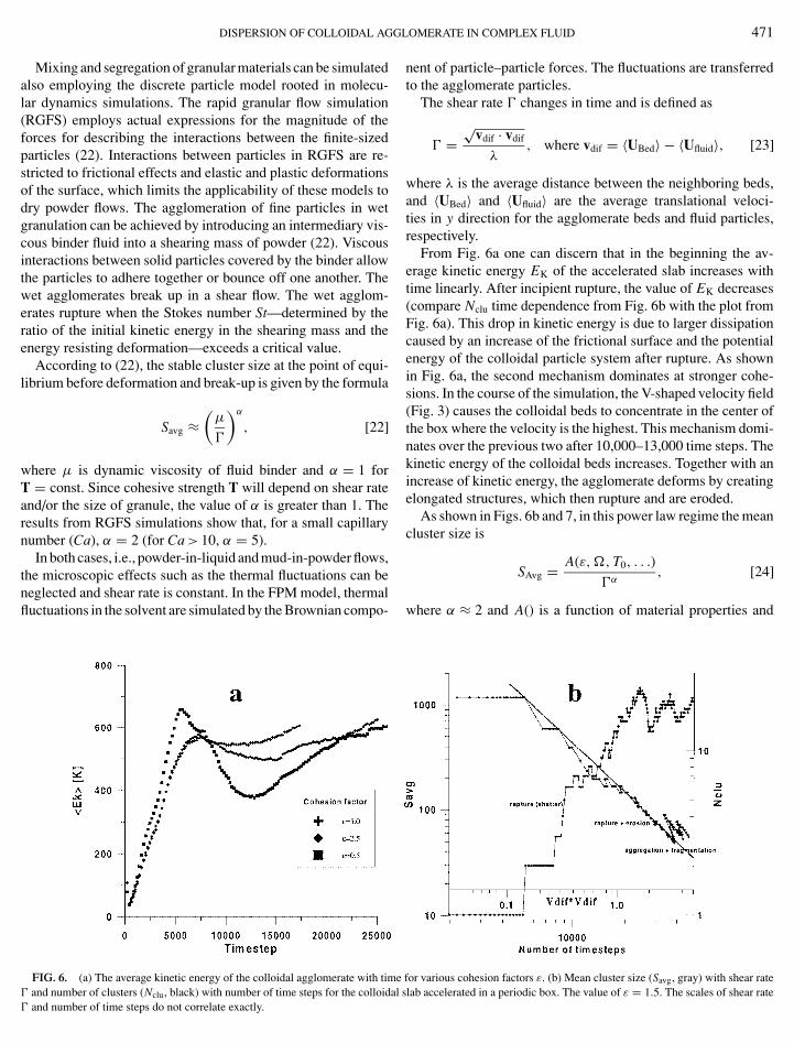

L

DISPERSION OF COLLOIDAL AGG

Mixing and segregation of granular materials can be simulatedalso employing the discrete particle model rooted in molecu-lar dynamics simulations. The rapid granular flow simulation(RGFS) employs actual expressions for the magnitude of theforces for describing the interactions between the finite-sizedparticles (22). Interactions between particles in RGFS are re-stricted to frictional effects and elastic and plastic deformationsof the surface, which limits the applicability of these models todry powder flows. The agglomeration of fine particles in wetgranulation can be achieved by introducing an intermediary vis-cous binder fluid into a shearing mass of powder (22). Viscousinteractions between solid particles covered by the binder allowthe particles to adhere together or bounce off one another. Thewet agglomerates break up in a shear flow. The wet agglom-erates rupture when the Stokes number St—determined by theratio of the initial kinetic energy in the shearing mass and theenergy resisting deformation—exceeds a critical value.

According to (22), the stable cluster size at the point of equi-librium before deformation and break-up is given by the formula

Savg ≈(

µ

�

)α

, [22]

where µ is dynamic viscosity of fluid binder and α = 1 forT = const. Since cohesive strength T will depend on shear rateand/or the size of granule, the value of α is greater than 1. Theresults from RGFS simulations show that, for a small capillarynumber (Ca), α = 2 (for Ca > 10, α = 5).

In both cases, i.e., powder-in-liquid and mud-in-powder flows,the microscopic effects such as the thermal fluctuations can be

neglected and shear rate is constant. In the FPM model, thermal fluctuations in the solvent are simulated by the Brownian compo-

FIG. 6. (a) The average kinetic energy of the colloidal agglomerate with time for various cohesion factors ε. (b) Mean cluster size (Savg, gray) with shear rate

where α ≈ 2 and A() is a function of material properties and

� and number of clusters (Nclu, black) with number of time steps for the colloidal� and number of time steps do not correlate exactly.

OMERATE IN COMPLEX FLUID 471

nent of particle–particle forces. The fluctuations are transferredto the agglomerate particles.

The shear rate � changes in time and is defined as

� =√

vdif · vdif

λ, where vdif = 〈UBed〉 − 〈Ufluid〉, [23]

where λ is the average distance between the neighboring beds,and 〈UBed〉 and 〈Ufluid〉 are the average translational veloci-ties in y direction for the agglomerate beds and fluid particles,respectively.

From Fig. 6a one can discern that in the beginning the av-erage kinetic energy EK of the accelerated slab increases withtime linearly. After incipient rupture, the value of EK decreases(compare Nclu time dependence from Fig. 6b with the plot fromFig. 6a). This drop in kinetic energy is due to larger dissipationcaused by an increase of the frictional surface and the potentialenergy of the colloidal particle system after rupture. As shownin Fig. 6a, the second mechanism dominates at stronger cohe-sions. In the course of the simulation, the V-shaped velocity field(Fig. 3) causes the colloidal beds to concentrate in the center ofthe box where the velocity is the highest. This mechanism domi-nates over the previous two after 10,000–13,000 time steps. Thekinetic energy of the colloidal beds increases. Together with anincrease of kinetic energy, the agglomerate deforms by creatingelongated structures, which then rupture and are eroded.

As shown in Figs. 6b and 7, in this power law regime the meancluster size is

SAvg = A(ε, �, T0, . . .)

�α, [24]

slab accelerated in a periodic box. The value of ε = 1.5. The scales of shear rate

472 DZWINEL A

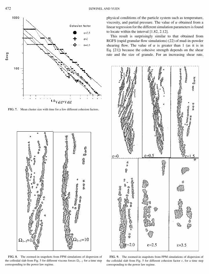
FIG. 7. Mean cluster size with time for a few different cohesion factors.

FIG. 8. The zoomed-in snapshots from FPM simulations of dispersion of

the colloidal slab from Fig. 5 for different viscous forces �1−1 for a time stepcorresponding to the power law regime.

ND YUEN

physical conditions of the particle system such as temperature,viscosity, and partial pressure. The value of α obtained from alinear regression for the different simulation parameters is foundto locate within the interval [1.82, 2.12].

This result is surprisingly similar to that obtained fromRGFS (rapid granular flow simulations) (22) of mud-in-powdershearing flow. The value of α is greater than 1 (as it is inEq. [21]) because the cohesive strength depends on the shearrate and the size of granule. For an increasing shear rate,

FIG. 9. The zoomed-in snapshots from FPM simulations of dispersion of

the colloidal slab from Fig. 5 for different cohesion factor ε, for a time stepcorresponding to the power law regime.

DISPERSION OF COLLOIDAL AGGLOMERATE IN COMPLEX FLUID 473

FIG. 10. The snapshot from simulation of accelerated colloidal slab in a tight box. More than one million particles (M = 106, M = 105) were employed.

The horizontal fluctuations caused by the reflecting walls generate the complex m

the temperature of a colloidal granule increases because theenergy from friction cannot be dissipated away. Thus, thereis a positive feedback, since the cohesive strength decreasessharply.

FIG. 11. The plot showing exponential dependence of the average clus-ter size on cohesion factor in the power law regime. Heterogeneous viscous

forces between colloidal beds and solvent droplets �1–2 influence the flowmuch stronger than viscous forces �1–2 of the fluid.

SP CP

ultiresolution patterns.

In Fig. 8 we present two snapshots from FPM simulations fordifferent �1–1, which stands for dissipative factor in the colloidalsystem. For smaller values of �1–1 dissipation is lower and thetemperature of the colloidal agglomerate becomes higher. The

FIG. 12. The average cluster size with viscous forces between colloidalbeds and solvent droplets �1–2.

474 DZWINEL A

FIG. 13. The zoomed-in snapshots from FPM simulations of dispersion ofthe colloidal slab from Fig. 5 for different viscous forces �1–2 for a time stepcorresponding to the power law regime.

FIG. 14. The zoomed-in snapshots from FPM simulations of dispersion of

the colloidal slab from Fig. 5 for the time steps corresponding respectively tothe power law and aggregation regimes.

ND YUEN

FIG. 15. The zoomed-in snapshots from FPM simulations of dispersion ofthe colloidal slab from Fig. 5 for different cohesion factor ε, for a time stepcorresponding to the aggregation regime.

cohesion decreases with temperature; thus, the mean cluster sizeis smaller. As in (21), one can roughly estimate that

A(ε, �, T0, . . .) ∝ f (�1−1), [25]

where f (�1–1) is a montonically increasing function of �1–1.As was depicted in Figs. 5, 7, and 9, the parameter

A(ε, �, T0, . . .) is also a function of cohesion factor ε. In thecase of ε = 0 the cohesion strength comes from viscous forces orit is of entropic origin (e.g., depletion forces). The agglomerateclusters create long threads (see Figs. 5, 9), which are parallel tothe streamlines even for a low shear rate. These threads are veryfragile and can easily be torn, for example, by the horizontalfluctuations caused by the reflecting walls. By simulatingensembles with many more particles, we can discern the act ofcreating very complex multiresolution structures (Fig. 10). Forgreater ε, we can observe that the structures become more rigidand compact and that the mean agglomerate size SAvg increases.

Let us now assume that the cohesive factor ε increases by dε.The change in energy d〈EB〉 supplied from the bulk of fluid tothe agglomerate of mean size SAvg must be compensated by thechange in potential energy d〈ES〉 on the agglomerate surfaceL (boundary in 2-D). This comes from an assumption that theenergy supplied is dissipated entirely in the agglomerate interior.Because 〈EB〉 should be proportional to the agglomerate surfaceand d〈ES〉 = Ldε, hence,

b1Ldε = d(b2L), [26]

DISPERSION OF COLLOIDAL AGGLOMERATE IN COMPLEX FLUID 475

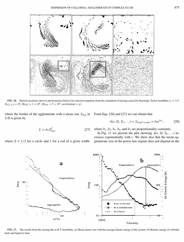
FIG. 16. Particle positions (above) and momenta (below) for selected snapshots from the simulation of mixing caused by Rayleigh–Taylor instability (ε = 3.5,

�12, 2–2 = 25, MTOT = 1 × 105, MCOL = 5 × 103, acceleration = g).

where the border of the agglomerate with a mean size SAvg in2-D is given by

L = b3Sβ

Avg, [27]

where β = 1/2 for a circle and 1 for a rod of a given width.creases exponentially with ε. We show also that the mean ag-glomerate size in the power law regime does not depend on the

FIG. 17. The results from the mixing due to R-T instability. (a) Mean cluster sbeds and liquid in time.

From Eqs. [26] and [27] we can obtain that

A(ε, �, T0, . . .) = SAvg|�=const = b5eb4ε, [28]

where b1, b2, b3, b4, and b5 are proportionality constants.In Fig. 11 we present the plot showing A(ε, �, T0, . . .) in-

ize with the average kinetic energy of the system. (b) Kinetic energy of colloidal

A

476 DZWINEL

solvent viscous forces represented by the dimensionless factor�2–2. We have checked that this relationship is also true forfluid with �2–2 ∈ [1, 90]. This fact stands in contradiction to theEq. [21] obtained for empirical data from rupture of the fractalagglomerate in a shear flow. Instead, we can observe in Fig. 12that SAvg decreases with the reciprocal of �1–2, which repre-sents direct dissipative interactions between colloidal beds andfluid particles. The effect of these interactions can be discerned

in Fig. 13. A greater value of �1–2 results in greater degree offragmentation and smaller value of SAvg. that for a longer simulation time the fragments of colloidal slab

FIG. 18. The snapshots from the simulation of mixing of colloidal beds in liquid caused by Rayleigh–Taylor instability. More than a million particles were4

simulated by including MCOL = 5 × 10 colloidal beds. The acceleration is eq

60,000 time steps, respectively.

ND YUEN

Finally, we can summarize that in the power law regime, themean agglomerate size decreases with shear rate � as

SAvg = b5 f (�1−1)eb4ε

�1−2�2. [29]

As shown in Fig. 6b, the linear regime is perturbed for largervalues of �. The colloidal beds concentrate in the center of thebox where the velocity is the highest. We display in Fig. 14

ual to 0.2 × g (see Table 2). The simulation time is T = 20,000, 40,000, and

the mean agglomerate size. From Fig. 15a it is apparent that the

DISPERSION OF COLLOIDAL AGG

create long threads. The threads break up and agglomerate dueto the convergent flow. The number of clusters (Ncl) fluctuatesin this regime (Fig. 6a).

Dissipative forces damp out the thermal fluctuations andfluctuations generated by the boundary conditions, which areresponsible for rupture. For larger value of the solvent viscos-ity represented by �2–2 the process of agglomeration is get-ting faster and the resulting structures are smoother than for alower viscosity. The effect can be observed by comparing Fig. 9(�2–2 = 15) and Fig. 15 (�2–2 = 45). The direct influence of thefragmentation and agglomeration on flow can also be discernedfor more complex types of flows.

5. DISPERSION PRODUCED BY MIXING INDUCEDBY RAYLEIGH–TAYLOR INSTABILITY

In (35, 36), we have employed the dissipative particle dy-namics approach to tackle the problem of mixing induced byRayleigh–Taylor instability at the mesoscale. We show that theinteractions between DPD particles and thermal fluctuations indissipative fluids influence strongly the speed of mixing. Theflow changes from rising mushrooms to bubble dynamics in-duced by the transformation to microscopic morphology, thebreaking-up of spikes, and the coalescence of the droplets.

We have simulated a Rayleigh–Taylor type of flow but for aliquid–solid system. The discrete particles are confined to move

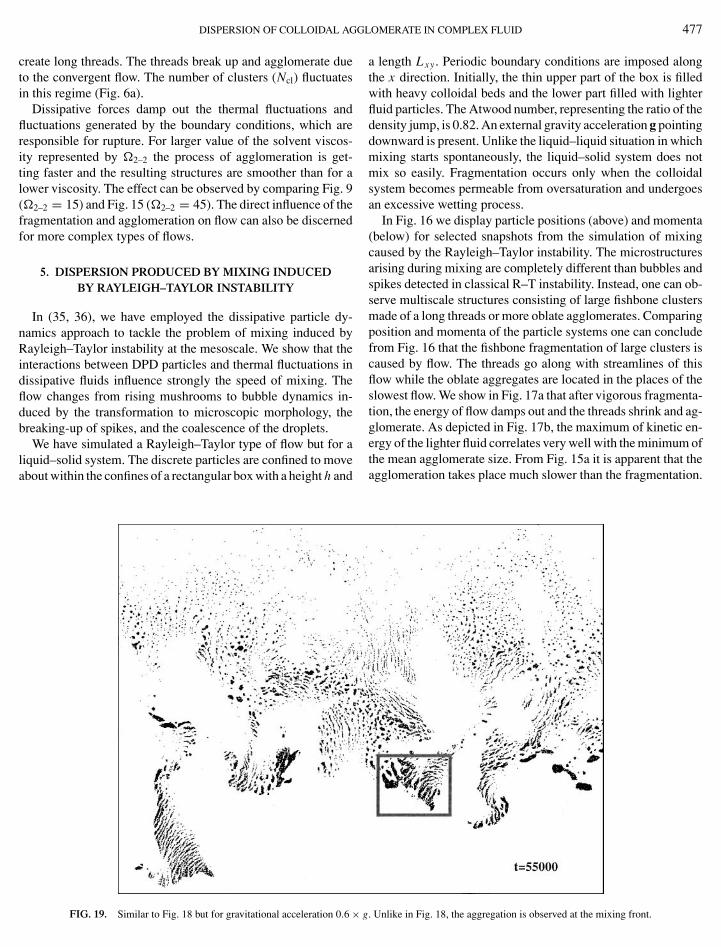
about within the confines of a rectangular box with a height h and agglomeration takes place much slower than the fragmentation.

FIG. 19. Similar to Fig. 18 but for gravitational acceleration 0.6 ×

LOMERATE IN COMPLEX FLUID 477

a length Lxy . Periodic boundary conditions are imposed alongthe x direction. Initially, the thin upper part of the box is filledwith heavy colloidal beds and the lower part filled with lighterfluid particles. The Atwood number, representing the ratio of thedensity jump, is 0.82. An external gravity acceleration g pointingdownward is present. Unlike the liquid–liquid situation in whichmixing starts spontaneously, the liquid–solid system does notmix so easily. Fragmentation occurs only when the colloidalsystem becomes permeable from oversaturation and undergoesan excessive wetting process.

In Fig. 16 we display particle positions (above) and momenta(below) for selected snapshots from the simulation of mixingcaused by the Rayleigh–Taylor instability. The microstructuresarising during mixing are completely different than bubbles andspikes detected in classical R–T instability. Instead, one can ob-serve multiscale structures consisting of large fishbone clustersmade of a long threads or more oblate agglomerates. Comparingposition and momenta of the particle systems one can concludefrom Fig. 16 that the fishbone fragmentation of large clusters iscaused by flow. The threads go along with streamlines of thisflow while the oblate aggregates are located in the places of theslowest flow. We show in Fig. 17a that after vigorous fragmenta-tion, the energy of flow damps out and the threads shrink and ag-glomerate. As depicted in Fig. 17b, the maximum of kinetic en-ergy of the lighter fluid correlates very well with the minimum of

g. Unlike in Fig. 18, the aggregation is observed at the mixing front.

478 DZWINEL A

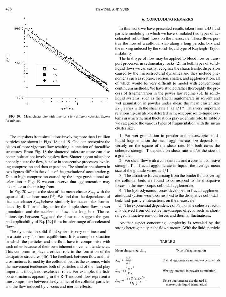
FIG. 20. Mean cluster size with time for a few different cohesion factorsfor mixing.

The snapshots from simulations involving more than 1 millionparticles are shown in Figs. 18 and 19. One can recognize theplaces of more vigorous flow resulting in creation of threadlikestructures. From Fig. 18 the shattered microstructure can alsooccur in situations involving slow flow. Shattering can take placenot only due to the flow, but also in consecutive processes involv-ing compression and then expansion. The simulations shown intwo figures differ in the value of the gravitational acceleration g.Due to high compression caused by the large gravitational ac-celeration in Fig. 19 we can observe that agglomeration maytake place at the mixing front.

In Fig. 20 we plot the size of the mean cluster SAvg with thesquared of the shear rate (�2). We find that the dependence ofthe mean cluster SAvg behaves similarly for the complex flow in-duced by R–T instability as for the simple shear flow in wetgranulation and the accelerated flow in a long box. The re-lationships between SAvg and the shear rate suggest the gen-eral applicability of Eq. [29] for a broader range of acceleratedflows.

The dynamics in solid–fluid system is very nonlinear and isin a state very far from equilibrium. It is a complex situationin which the particles and the fluid have to compromise witheach other because of their own inherent movement tendencies.This compromise plays a critical role in the formation of thedissipative structures (46). The feedback between flow and mi-crostructures formed by the colloidal beds is the extreme, whilethe movement tendencies both of particles and of the fluid playimportant, though not exclusive, roles. For example, the fish-bone structures appearing in the R–T induced flow represent a

true compromise between the dynamics of the colloidal particlesand the flow induced by viscous and inertial effects.

ND YUEN

6. CONCLUDING REMARKS

In this work we have presented results taken from 2-D fluidparticle modeling in which we have simulated two types of ac-celerated solid–fluid flows on the mesoscale. These flows por-tray the flow of a colloidal slab along a long perodic box andthe mixing induced by the solid–liquid type of Rayleigh–Taylorinstability.

The first type of flow may be applied to blood flow or trans-port processes in sedimentary rocks (2). In both types of solid–liquid flows we can easily recognize the characteristic dispersioncaused by the microstructural dynamics and they include phe-nomena such as rupture, erosion, shatter, and agglomeration, allof which would be very difficult to model with conventionalcontinuum methods. We have studied rather thoroughly the pro-cess of fragmentation in the power law regime (3). In solid–liquid systems, such as the fractal agglomerate in solvent andwet granulation in powder under shear, the mean cluster sizeSAvg varies with the shear rate � as 1/�α . This very importantrelationship can also be detected in mesoscopic solid–liquid sys-tems in which thermal fluctuations play a definite role. In Table 3we categorize the various types of fragmentation with the meancluster size.

1. For wet granulation in powder and mesoscopic solid–liquid fragmentation the mean agglomerate size depends in-versely on the square of the shear rate. For both cases thecohesive strength T depends on shear rate and/or the size ofa granule.

2. For shear flow with a constant rate and a constant cohesivestrength T in fractal agglomerate-in-liquid, the average meansize of the granule varies as 1/�.

3. The attractive forces arising from the binder fluid coveringthe colloidal beds are found to correspond to the dissipativeforces in the mesoscopic colloidal agglomerate.

4. The hydrodynamic forces developed in fractal agglomer-ate/liquid system would correspond to the dissipative colloidal–bed/fluid–particle interactions on the mesoscale.

5. The exponential dependence of SAvg on the cohesive factorε is derived from collective mesoscopic effects, such as short-ranged, attractive ion–ion forces and thermal fluctuations.

Another aspect concerning complexity is revealed by thestrong heterogeneity in the flow structure. With the fluid–particle

TABLE 3

Mean cluster size, SAvg Type of fragmentation

Savg ≈ g(ε)

µ�Fractal agglomerate in fluid (experimental)

Savg ≈(

µ

�

)2

Wet agglomerate in powder (simulation)

Savg = b5 f (�1–1)eb4ε

2Dense agglomerate accelerated in

�1–2� mesoscopic liquid (simulation)

L

DISPERSION OF COLLOIDAL AGG

model one can discern properly the mutilscale character of thesolid–fluid system. As shown in Fig. 18, multiresolution struc-tures prevail in a solid–fluid system. These multiscale structuresare complicated due to the inflexibility of the description levelwith varying scale of observation. Unlike in (46), where differentnumerical methods were employed for describing the particle,the cluster, and the entire system, the FPM model is the solenumerical paradigm in our simulations. From a computationalstandpoint, we do not observe any methodological disparity ofsolid–fluid interaction mechanisms in totally different regimesin which either fluids or particles may dominate.

Even though the fluid–particle model is superior to the oldermesoscopic scheme—dissipative particle dynamics—it does notsolve the serious conceptual problem of the method of DPD. Thethermodynamic behavior of the fluid particle model is deter-mined by the conservative forces, which are soft in comparisonwith the singular MD interactions. Hence, there does not exista well-defined procedure to relate the shape and amplitude ofthe conservative forces with a prescribed thermodynamic behav-ior. Furthermore, it is not clear what physical time and lengthscales the model actually describes. The presence of thermalnoise suggests a fuzzy area belonging to the mesoscopic realm.In (30) we show, for example, that the DPD and FPM fluid struc-tures resemble short-chain polymers. In (47) it is proved that thespatiotemporal scale for DPD can be precisely defined by in-troducing the volume of a fluid particle as a new variable. Themodel is interesting from a theoretical point of view but it is veryhard for implementing efficiently in simulating multicomponentfluids. Moreover, it is less efficient involving a larger cut-off ra-dius than FPM and DPD. This price paid for being more strictwith matching the spatiotemporal scale may appear currentlytoo demanding, especially for 3-D simulations (48). There is athin border between the applicability of a numerical model andthe theory.

With the FPM we can extend further the capabilities of thediscrete particle method to the mesoscopic regime and showthat they are competitive to standard simulation techniques withcontinuum equations. These methods establish a foundation forcross-scale computations ranging from nanoscales to micronsand can provide a framework to study the interaction of mi-crostructures and large-scale flow, which may be of value inblood flow and other applications in polymeric dynamics.

ACKNOWLEDGMENTS

We thank Dr. Dan Kroll (MSI) for useful discussions. Support for this workwas provided by the Energy Research Laboratory Technology Research Pro-gram of the Office of Energy Research of the U.S. Department of Energy undersubcontract from the Pacific Northwest National Laboratory and partly by thePolish Committee for Scientific Research (KBN).

REFERENCES

1. Moseler, M., and Landman, U., Science 289, 1165–1169 (2000).2. Olson, J. F., and Rothman, D. H., J. Fluid Mech. 341, 343–365 (1997).

OMERATE IN COMPLEX FLUID 479

3. Ottino, J. M., De Roussel, P., Hansen, S., and Khakhar, D. V., Adv. Chem.Eng. 25, 105–204, (2000).

4. Prausnitz, J., and Wu, J., En Vision 16, 18–19 (2000).5. Gast, A. P., and Russel, W. B., Phys. Today December, 24–30 (1998).6. Burda, P., and Korenar, J., Akad. Verlag. Z. Angew. Math. Mechan. 76,

365–366 (1996).7. Gueraoui, K., Hammoumi, A., and Zeggwagh, G., C. R. Acad. Sci. Ser.

Fascicule B-Mecanique Phys. Chim. Astron. 326, 561–568 (1998).8. Latinopoulos, P., and Ganoulis, J., Appl. Math. Modelling 6, 55–60 (1982).9. Misra, J. C., and Sahu, B. K., Comput. Math. Appl. 16, 993–1016 (1988).

10. Groisman, A., and Stainberg, V., Nature 405, 53–55 (2000).11. Fung, Y. C., and Zweifach, B. W., Annu. Rev. Fluid Mechanics III, 189–210

(1971).12. Alda, W., Dzwinel, W., Kitowski, J., Moscinski, J., Pogoda, M., and Yuen,

D. A., Comput. Phys. 12, 6, 595–600 (1998).13. Dzwinel, W., Alda, W., Pogoda, M., and Yuen, D. A., Physica D 137, 157–

171 (2000).14. Vashishta, P., and Nakano, A., Comput. Sci. Eng. Sept/Oct, 20–23 (1999).15. Chopard, B., and Droz, M., “Cellular Automata Modelling of Physical

Systems,” Cambridge Univ. Press, Cambridge, UK, 1998.16. Swift, M. R., Orlandini, E., Osbors, W. R., and Yeomans, J. M., Phys. Rev.

E 54, 5041–5052 (1996).17. Wagner, A. J., and Yeomans, J. M., submitted for publication. 2000.18. Meakin, P., “Fractals, scaling and growth far from equilibrium,” Cambridge

Univ. Press, Cambridge, UK, 1998.19. Choi, H. G., and Joseph, D. D., Fluidization by Lift of 300 Circular Parti-

cles in Plane Poiseuille Flow by Direct Numerical Simulation, Universityof Minnesota Supercomputing Institute Research Report, UMSI 2000/17,February 2000.

20. Glowinski, R., Pan, T. W., Hela, T. I., Joseph, D. D., and Priaux, J., AFictitious Domain Approach to the Direct Numerical Simulation of Incom-pressible Viscous Flow Past Moving Rigid Bodies: Application to ParticleFlow, University of Minnesota Supercomputing Institute Research Report,UMSI 2000/68, April 2000.

21. Ihle, T., and Kroll, D. M., Phys. Rev. E 63/2, 201 (2001).22. Talu, I., Tardos, G. I., and Khan, M. I., Powder Technol. 110, 59–75

(2000).23. Hoogerbrugge, P. J., and Koelman, J. M. V. A., Europhys. Lett. 19, 155–160

(1992).24. Espanol, P., Phys. Rev. E 57, 2930–2948 (1998).25. Marsh, C., Backx, G., and Ernst, M. H., Phys. Rev. E 56, 1976 (1997).26. Groot, R. D., and Warren, P. B., J. Chem. Phys. 107, 4423 (1997).27. Whittle, M., and Dickinson, E., J. Colloid Interface Sci. 242, 106–109

(2001).28. Clark, A. T., Lal, M., Ruddock, J. N., and Warren, P. B., Langmuir 16,

6342–6350 (2000).29. Coveney, P. V., and Novik, K. E., Phys. Rev. E 54(5), 5134–5141 (1996).30. Dzwinel, W., and Yuen, D. A., Int. J. Modern Phys. C 11, 1–25 (2000).31. Dzwinel, W., and Yuen, D. A., J. Colloid Interface Sci. 225, 179–190

(2000).32. Dzwinel, W., and Yuen, D. A., Int. J. Modern Phy. C 11, 1037–1062 (2000).33. Dzwinel, W., and Yuen, D. A., Mol. Simul. 22, 369–395 (1999).34. Boryczko, K., Dzwinel, W., and Yuen, D. A., Mixing and droplets co-

alescence in immiscible fluid. 3-D dissipative particle dynamics model,Minnesota Supercomputing Institute Research Reports, UMSI 2000/142,July 2000 and Proceedings of 1st SGI Users Conference, Cracow, Poland,October 2000, ACC Cyfronet UMM, 231–240, 2000.

35. Dzwinel, W., and Yuen, D. A., Int. J. Modern Phys. C 12, 91–118 (2001).36. Dzwinel, W., Yuen, D. A., and Boryczko, K., J. Mol. Modeling, in press,

(2002).37. Libersky, L. D., Petschek, A. G., Carney, T. C., Hipp, J. R., and Allahdadi,

F. A., J. Comp. Phys. 109, 67–73 (1993).38. Daniel, J. C., and Audebert, R., Small Volumes and Large Surfaces: The

World of Colloids, in “Soft Matter Physics” (M. Daoud and C. E. Williams,Eds.), p. 320, Springer Verlag, Berlin, 1999.

480 DZWINEL A

39. Grier, D. G., and Behrens, S. H., Interactions in colloidal suspensions, in“Electrostatic effects in Soft Matter and Biphysics” (C. Holm, P. Keikchoff,and R. Podgornik, Eds.), Kluwer, Dordrecht, 2001.

40. Yaman, K., Jeppesen, C., and Marques, C. M., Europhys. Lett. 42, 221–226(1998).

41. Larsen, A., and Grier, D. G., Nature 385, 230–233 (1997).42. Hockney, R. W., and Eastwood, J. W., “Computer Simulation Using

Particles,” McGraw-Hill Inc., New York, 1981.43. Kubo, R., “Statistical Mechanics,” Wiley, New York, 1965.

ND YUEN

44. Chapman, S., and Cowling, T. G., “The Mathematical Theoryof Non-uniform Gases,” Cambridge Univ. Press, Cambridge, UK,1990.

45. Serrano, M., and Espanol, P., Phys. Rev. E 6404(4), 6115 (2001).46. Li, J., Powder Technol. 111, 50–59 (2000).47. Espanol, P., Serrano, M., and Ottinger, H. Ch., Phys. Rev. Lett. 83, 4542–

4545 (1999).

48. Boryczko, K., Dzwinel, W., and Yuen, D. A., J. Concurrency: Practice

Experience 14, (2002).