Mesoscale Benchmark Demonstration - Pacific … · Mesoscale Benchmark Demonstration ... and Oak...

Mesoscale Benchmark Demonstration Problem 1: Mesoscale Simulations of Intra-

granular Fission Gas Bubbles in UO2 under Post-

irradiation Thermal Annealing

Prepared for

U.S. Department of Energy

Fuel Cycle R&D Program

Yulan Li, Shenyang Hu, Robert Montgomery, Fei Gao, Xin Sun

Pacific Northwest National Laboratory, Richland, WA 99352

Michael Tonks, Bulent Biner, Paul Millett

Idaho National Laboratory, Idaho Falls, ID 83415

Veena Tikare

Sandia National Laboratory, Albuquerque, NM 87185

Balasubramaniam Radhakrishnan

Oak Ridge National Laboratory, Oak Ridge, TN 37831

David Andersson

Los Alamos National Laboratory, Los Alamos, NM 87545

April 2012

FCR&D-MDSM-2012-000098

PNNL-21295

DISCLAIMER This information was prepared as an account of work sponsored by an agency of the U.S. Government. Neither the U.S. Government nor any agency thereof, nor any of their employees, makes any warranty, expressed or implied, or assumes any legal liability or responsibility for the accuracy, completeness, or usefulness, of any information, apparatus, product, or process disclosed, or represents that its use would not infringe privately owned rights. References herein to any specific commercial product, process, or service by trade name, trade mark, manufacturer, or otherwise, does not necessarily constitute or imply its endorsement, recommendation, or favoring by the U.S. Government or any agency thereof. The views and opinions of authors expressed herein do not necessarily state or reflect those of the U.S. Government or any agency thereof.

Mesoscale Benchmark Demonstration April 2012 iii

Reviewed by:

National Technical Director, Nuclear Energy

Advanced Modeling and Simulation

Keith Bradley Date

Concurred by:

Acting Director, Advanced Modeling and

Simulation Office

Trevor Cook Date

Approved by:

Deputy Assistant Secretary, Nuclear Energy

John Kelly Date

Mesoscale Benchmark Demonstration April 2012 iv

Mesoscale Benchmark Demonstration Problem 1: Mesoscale Simulations of Intra-granular Fission Gas

Bubbles in UO2 under Post-irradiation Thermal Annealing

SUMMARY

A study was conducted to evaluate the capabilities of different numerical methods used to represent microstructure behavior at the mesoscale for irradiated material using an idealized benchmark problem. The purpose of the mesoscale benchmark problem was to provide a common basis for assessing several mesoscale methods to identify the strengths and areas of improvement in the predictive modeling of microstructure evolution. In this work, mesoscale models (phase-field, Potts, and kinetic Monte Carlo) developed by Pacific Northwest National Laboratory, Idaho National Laboratory, Sandia National Laboratory, and Oak Ridge National Laboratory were used to calculate the evolution kinetics of intra-granular fission gas bubbles in UO2 fuel under post-irradiation thermal annealing conditions. The benchmark problem was constructed to include important microstructural evolution kinetics of intra-granular fission gas bubble behavior, such as the atomic diffusion of Xe atoms, U vacancies, and O vacancies; the effect of vacancy capture and emission from defects; and the elastic interaction on non-equilibrium gas bubbles. An idealized set of assumptions and a common set of thermodynamic and kinetic data were imposed on the benchmark problem to simplify the mechanisms considered. The modeling capabilities of different methods are compared against selected experimental and simulation results. These comparisons find that while the phase-field methods and Potts kinetic Monte Carlo methods are able to incorporate several of the mechanisms that influence intra-granular bubble growth and coarsening, the Potts model is challenged by the low solubility and long-range diffusion necessary to simulate this problem correctly. The statistical-mechanical nature of Potts kMC requires large ensembles with long simulation times to treat this problem. Future efforts are recommended to construct increasingly more complex mesoscale benchmark problems to further verify and validate the predictive capabilities of the mesoscale modeling methods used in this study.

Key words: mesoscale benchmark; phase-field approach; kinetic Monte Carlo approach; Potts model; fission gas bubbles; uranium dioxide; post-irradiation thermal annealing.

Mesoscale Benchmark Demonstration April 2012 v

CONTENTS

SUMMARY .................................................................................................................................................... IV

ACRONYMS ................................................................................................................................................ VIII

1. INTRODUCTION .................................................................................................................................... 1

1.1 Study Purpose and Scope ................................................................................................................ 3

1.2 Report Contents and Organization .................................................................................................. 3

2. MICROSTRUCTURE BEHAVIOR IN IRRADIATED UO2 MATERIALS .......................................... 4

2.1 Fission Gas Behavior in UO2 Fuel .................................................................................................. 4

2.2 Intra-granular Fission Gas Atom Behavior ..................................................................................... 5

3. DESCRIPTION OF THE MESOSCALE BENCHMARK PROBLEM ................................................... 8

3.1 Thermodynamic and Kinetic Properties of Defects in UO2 .......................................................... 10

3.1.1 Oxygen interstitials and vacancies .................................................................................... 10

3.1.2 Uranium interstitials and vacancies ................................................................................... 10

3.1.3 Fission gas ......................................................................................................................... 10

3.2 Assessment of the Thermodynamic Parameters ............................................................................ 12

4. SUMMARY OF MESOSCALE METHODS AND BENCHMARK PROBLEM RESULTS ............... 13

4.1 Mesoscale Methods ....................................................................................................................... 13

4.1.1 Phase-field model used by PNNL ..................................................................................... 14

4.1.2 Phase-field model used by INL ......................................................................................... 16

4.1.3 Potts model used by SNL .................................................................................................. 17

4.1.4 kMC model used by ORNL ............................................................................................... 19

4.2 Summary of Different Methods and Simulation Results ............................................................... 20

4.2.1 Results from PNNL’s phase-field modeling ..................................................................... 22

4.2.2 Results from INL’s phase-field modeling ......................................................................... 28

4.2.3 Results from SNL’s Potts modeling .................................................................................. 31

4.2.4 Results from ORNL’s Potts/kMC modeling ..................................................................... 35

4.3 Assessment of Mesoscale Modeling Methods ............................................................................... 37

5. MAIN CONCLUSIONS AND FUTURE WORK ................................................................................. 41

6. ACKNOWLEDGMENTS ...................................................................................................................... 42

7. APPENDIXES ........................................................................................................................................ 42

REFERENCES ................................................................................................................................................ 43

FIGURES

Figure 1. Schematic process of thermally induced fission gas diffusion and release from fuels. ..................... 5

Figure 2. Intra-granular bubble behavior from Kashibe et al. [26]. .................................................................. 6

Figure 3. Burnup dependence of mean diameter and number density after annealing at 1800°C for 5 hours. (*) Annealing at 1700°C C-1800°C C for ~60 minutes [26]. ............................................................ 7

Figure 4. (a) Concentration and elastic interaction dependence of gas bubble critical size, and (b) pressure and shear stress around the gas bubble. .......................................................................................... 13

Mesoscale Benchmark Demonstration April 2012 vi

Figure 5. (a) Gas bubble density in a function of gas bubble mean diameter, (b) gas bubble volume fraction

vs time, and (c) time evolution of gas bubble morphology for the case 001.00 vc with elastic

interaction. ...................................................................................................................................... 24

Figure 6. Gas bubble density in a function of gas bubble mean diameter. ..................................................... 25

Figure 7. Gas bubble morphology a) and b) with vacancy emissions from different distributed dislocations. The light blue dots denote the location of dislocations while the black circles identify the initial gas bubbles. The framed parts illustrate the obvious difference due to the local emission of vacancies. ....................................................................................................................................... 26

Figure 8. Evolution of bubble number and bubble gas atom volume fraction with time. ............................... 27

Figure 9. Comparison of gas bubble density vs mean diameters from PF modeling and experiments. .......... 27

Figure 10. Images of the bubble growth during the annealing of the 10-nm thickness 2-D simulation. Note that the adapted mesh is also shown in the simulations. The initial condition of the 3-D simulation is also shown. ................................................................................................................ 28

Figure 11. Post-irradiation annealing results, with the average bubble radius vs. time on the left and the bubble density vs. time on the right. ............................................................................................... 29

Figure 12. Gas bubble density as a function of the gas bubble mean diameter, comparing the experimental fit from Kashibe et al. [26] to our 2-D and 3-D simulation results. The 3-D results are a better fit with the experimental fit. ................................................................................................................ 29

Figure 13. The results of mesh and time step adaptivity for the 10-nm thickness 2-D simulation, where (a) shows the decrease in the number of degrees of freedom with time due to adapting the mesh, with the number of bubbles shown for reference, and (b) shows the time step size with time, with the inverse of the diffusion constant shown for reference. ............................................................. 30

Figure 14. Investigation of the effect of the initial condition of the bubbles using a 100-nm by 100-nm 2-D domain, where (a) shows the effect of the variation in the bubble position and (b) the effect of variation in the bubble radius. ........................................................................................................ 31

Figure 15. Microstructure of bubbles coarsening (only a portion of the simulation space is imaged, 2003 l3 corresponding to 40 nm x 40 nm x 40 nm). .................................................................................... 32

Figure 16. Average bubble radius as a function of time. ................................................................................ 33

Figure 17. Bubble size distributions as the bubbles coarsen. .......................................................................... 34

Figure 18. Bubble growth kinetics in a 416- x 416- x 416-nm3 simulation volume. ...................................... 35

Figure 19. Bubble size distribution obtained using the 416- x 416- x 416-nm3 run. ...................................... 36

Figure 20. Temporal evolution of the bubbles in the 416- x 416- x 416-nm3 run showing the migration and coalescence mechanism operating throughout the simulation time. ............................................... 37

Figure 21. Trend in bubble density versus mean bubble diameter for intra-granular bubble growth and coarsening during post-irradiation annealing. Comparison of results from mesoscale methods and experimental data is indicated. ................................................................................................. 39

TABLES

Table 1. Initial condition of intra-granular fission gas bubble coalescence during thermal annealing. ............ 9

Table 2. Thermodynamic and kinetic properties of defects in UO2x . ........................................................... 11

Table 3. Initial condition used in simulations. ................................................................................................ 20

Table 4. Thermodynamic and kinetic properties of defects in UO2 used in simulations. ............................... 21

Table 5. Computation efforts made in the simulations. .................................................................................. 21

Table 6. Mechanisms considered in the simulations....................................................................................... 22

Mesoscale Benchmark Demonstration April 2012 vii

Table 7. CPU time with 2.66-GHz core for 10,000 simulation time steps. .................................................... 27

Mesoscale Benchmark Demonstration April 2012 viii

ACRONYMS

°C degree(s) Celsius or Centigrade

2-D two-dimensional (or two dimensions)

3-D three-dimensional (three dimensions)

Å3 cubic Angstrom

C constant temperature

CPU central processing unit

DFT Density Functional Theory

DOF degrees of freedom

eV electron volt

FEM finite element method

FFTW Fastest Fourier Transform in the West

GPa Giga pascal

GWd/MTU gigawatt-days per metric ton uranium

h hour(s)

INL Idaho National Laboratory

J/m2 joule per square meter

K Kelvin

kMC kinetic Monte Carlo

Kr krypton

LANL Los Alamos National Laboratory

LWR light water reactor

min minute(s)

MD molecular dynamics

MCS Monte Carlo time

O oxygen

ORNL Oak Ridge National Laboratory

PF phase-field

PNNL Pacific Northwest National Laboratory

R ramp temperature

s or sec second(s)

SNL Sandia National Laboratory

U uranium

UO2 uranium dioxide

Xe xenon

Mesoscale Benchmark Demonstration April 2012 1

FUEL CYCLE R&D PROGRAM

MESOSCALE BENCHMARK DEMONSTRATION

PROBLEM 1: MESOSCALE SIMULATIONS OF INTRA-GRANULAR FISSION GAS BUBBLES IN UO2 UNDER POST-IRRADIATION THERMAL ANNEALING

1. INTRODUCTION Computational materials science—an active research area under intensive development in recent years— promises to provide improved and predictive capability for the modeling and simulation of material microstructural, mechanical, and thermal behaviors under extreme environmental conditions. The ability to describe and model the complex behavior of materials from the atomistic to the continuum scales can provide opportunities to design new materials and better understand and use existing materials. In general, computational materials models can be categorized into three groups based on their temporal and spatial domains of interest: at the atomistic scale, models include density functional theory (DFT) [1-4] and molecular dynamics (MD) methods [5-10]; at the mesoscale (i.e., microstructure level), models include the kinetic Monte Carlo (kMC) (i.e., Potts model) [11], and the phase-field (PF) methods [12-15]; at the continuum scale, methods include the finite element [16] and finite volume methods [17, 18].

A key challenge in modeling material behavior using the described multi-scale approach is the bridging or transfer of information across the disparate time and spatial scales of importance. Modeling within the atomistic domain considers at most microseconds and nanometers (millions of atoms and their motion) in describing atomic or molecular interactions. The continuum domain modeling can stretch to years and centimeters in the case of nuclear fuel rods or irradiated material. Given the large disparities between these domains, mesoscale methods may play a key role in bridging the temporal and spatial scales in computational materials science and may provide methods to better inform the constitutive models used at the continuum scale.

The atomistic and continuum domains are mature areas of computational materials science modeling with established confidence in the ability of their methods to provide predictive simulations, using, in the case of continuum level, semi-empirical constitutive models that may include lower length scale properties (e.g., diffusivities or Burger’s vector). In contrast, the mesoscale domain of materials modeling is a relatively new area of development in computational materials science that resides between the discrete atomic particle models and the continuum representation. The characteristic length scales generally range from 100s of nanometers to 10s of micrometers and time scales of 10-3 to 102 seconds. At these scales, the domain is often too small to be considered a continuum level representation, yet too large to effectively use atomistic methods. The advantage of the mesoscale modeling domain lies in the fact that microstructure-level material characteristics such as inhomogeneity, i.e., grains, grain boundaries or other

Problem 1: Mesoscale Simulations of Intra-granular Fission Gas Bubbles in UO2 under Post-irradiation Thermal Annealing

2 April 2012

defects, can be represented in local detail and their interactions with atomic processes can be explicitly considered. These microstructural features have a deciding impact on material behavior on the continuum scale. Various mesoscale modeling methods have been successfully demonstrated to topographically represent the evolution of material microstructure during grain growth, sintering, and migration of bubbles within the solid. However, an important gap in the various mesoscale modeling methods is the lack of quantitative verification and validation in predicting microstructure evolution kinetics with quantitative inputs from the atomistic scale, particularly under complex conditions of temperature, strain, and radiation damage.

Several mesoscale modeling methods have been developed to evaluate microstructure evolution during the process of grain growth, phase transformation, second phase particle growth, etc. [12, 14, 15, 19]. The most widely used and well-known mesoscale modeling methods used in computational materials science are the Potts, kMC, and the PF approaches. The first two methods are discrete ensemble representations that use a statistical-mechanical approach to represent the evolution of distinct interfaces in the microstructure. The PF approach is a thermodynamic model that represents the microstructure using a continuum field with a set of smoothly changing order parameters to define the interfaces. Each of these methods has been successfully used to simulate microstructure evolution in metal and ceramic materials under conditions without irradiation. Tikare et al. [20] have compared the Potts and PF methods for grain growth simulations and Ostwald ripening processes. For these single-mechanism simulations, both methods gave similar topological results.

Application of mesoscale methods to predict microstructure evolution driven by complex and interacting mechanisms, such as those that occur in nuclear fuel under irradiation, has grown recently with the advancement of computational capabilities and the desire to improve the semi-empirical material models used in representing these systems. The ultimate goal in applying mesoscale methods to irradiated materials is to develop a quantitative, mechanistic-based multi-physics representation of the underlying processes controlling the microstructure evolution for predicting the material properties evolution at the continuum scale, i.e., thermal conductivity, elastic modulus, creep, and behavior of second phase particles or fission products. For example, the migration of fission gas atoms in nuclear fuel material is influenced by several important microstructural mechanisms, including 1) gas atom diffusion, 2) gas atom or vacancy trapping by defects and dislocations, 3) interaction with fission fragments and fission-induced cascades, 4) nucleation and growth of gas bubbles, 5) absorption and resolution from gas bubbles, 6) non-equilibrium pressure conditions in gas bubbles, and 7) elastic interactions between defects and bubbles. All of these mechanisms have a combined effect in controlling the rate of gas atom diffusion to the grain boundary and its ultimate release from the fuel. Semi-empirical continuum-level models approximate all of these mechanisms into a single effective diffusivity with limited predictive capability.

As the complexity of microstructure modeling has grown, verifying the predictive capabilities of mesoscale methods becomes more difficult, and those conducting the exercises used to validate the results must have a deep understanding of the interacting mechanisms that control the microstructural data. Very few separate effect experiments are available to provide the microstructure characteristics in sufficient detail to quantitatively verify the mesoscale methods. As a result, a concerted effort is required to engage a spectrum of experts who understand the intricacies of the experimental data, the current knowledge of


the microstructure evolution kinetics, and the different continuum and mesoscale modeling methods in order to formulate the verification and validation problems that can truly evaluate the predictive capabilities of these methods.

1.1 Study Purpose and Scope This report describes a study undertaken to evaluate the capabilities of different methods used to represent microstructure behavior at the mesoscale for irradiated material using an idealized benchmark problem. The goal of developing such a benchmark problem is to provide a common basis for assessing the strength and areas of improvement for several different mesoscale methods in predicting the microstructure evolution of nuclear fuel material. The different mesoscale methods considered in this study include the PF method, Potts model, and kMC approaches. The benchmark problem summarized in this report is related to the growth and coarsening behavior of intra-granular fission gas bubbles observed after a post-irradiation thermal annealing test for uranium dioxide (UO2), and it is the first in a series of verification problems that will be constructed to begin the process of quantitative verification of mesoscale methods for predicting microstructure evolution. It is envisioned that additional test problems will be constructed and analyzed that involve increasingly more complex multi-physics behavior, including defect-dislocation interactions and fission-induced damage.

A multi-laboratory team of researchers from Pacific Northwest National Laboratory (PNNL), Idaho National Laboratory (INL), Sandia National Laboratory (SNL), Oak Ridge National Laboratory (ORNL), and Los Alamos National Laboratory (LANL) participated in the benchmark problem by performing analyses with various mesoscale methods as part of this study. An important aspect of defining a common benchmark problem was to establish a consistent set of initial, boundary, and thermodynamic conditions across the selected mesoscale methods.

1.2 Report Contents and Organization The ensuing sections of this report begin by describing the microstructure behavior of irradiated UO2 material and the relevant aspects that will be considered in the mesoscale benchmark problem (Section 2). Section 3 outlines the benchmark problem definition, including the initial, boundary, and thermodynamic conditions. It also includes a set of calculations performed to verify that the formulation of the different interacting mechanisms on the bubble growth behavior is reasonable. Section 4 summarizes the mesoscale methods used in the evaluation and a comparison of the assumptions and results between the different approaches. Areas of common agreement and areas for further improvement are identified. Section 5 discusses the key conclusions from this evaluation and provides suggestions for further analytical evaluation and experimental data generation. Detailed descriptions of the mesoscale methods used in this evaluation and the detailed results for the benchmark problem are contained in appendixes.


4 April 2012

2. MICROSTRUCTURE BEHAVIOR IN IRRADIATED UO2 MATERIALS

The thermal, mechanical, and chemical behavior of nuclear fuel material during normal operations and transient conditions is an important element of the performance, reliability, and safety of any nuclear reactor. Implicit in this behavior is the changing microstructure of the material as a consequence of radiation damage, fission product generation, temperature and stress fields, etc. Understanding the impact of the microstructure evolution on the material properties such as thermal conductivity, elastic modulus, creep, and fission product retention is critical to evaluating the performance of the fuel material. Extensive experimental and analytical work has been conducted to develop this understanding. What is known is that the evolving state of the microstructure and its impact on material properties in irradiated material is a complex multi-scale and multi-physics process composed of many interacting and competing mechanisms, including radiation-induced defects, moving grain boundaries, gas bubbles and porosity, fission product compounds, non-stoichiometry, etc. [21-24].

2.1 Fission Gas Behavior in UO2 Fuel During irradiation of light water reactor (LWR) fuel, the fission process generates many different fission product atoms, including xenon (Xe) and krypton (Kr) atoms. The noble gas atoms Xe and Kr represent about 30% of the fission products produced, and the behavior of the gas atoms is important to the microstructure evolution and overall performance of the fuel. Because of the extremely low solubility of the noble gas atoms in the UO2 matrix, gas bubbles composed of Xe , Kr, and other gas atoms precipitate within the UO2 grains and, depending on the temperature conditions, gas atom diffusion will result in nucleation and growth of gas bubbles on the grain boundaries. Continuum-level mechanisms, such as fission gas release to the fuel rod environment and volumetric swelling due to bubble growth, are included in nuclear fuel performance assessments.

The behavior of fission gas atoms in UO2 has been extensively studied using experiments performed on single crystal and polycrystalline material under a variety of temperature and irradiation conditions for more than 50 years [21, 24-29]. From these studies a general picture of the mechanisms that influence the transport and release of fission gas atoms has been developed. Thermally induced fission gas diffusion and release from the fuel generally occurs in two stages: 1) diffusion and trapping of single Xe gas atoms within the grains, and 2) formation and inter-linkage of grain boundary bubbles. A schematic of these processes is shown in Figure 1. First, a gas atom is created within a region of radiation-induced vacancies and interstitial atoms caused by the atomic interactions/cascades during the stopping process following fission. Gas atom diffusion assisted by uranium (U) vacancy clusters then takes over until nucleation of small high pressure intra-granular bubbles. These bubbles act as trapping sites for gas atoms until a fission fragment spike causes resolution of Xe atoms back into the matrix. Several transmission electron microscopy studies of irradiated fuel have found that the mean radius of the intra-granular bubbles is approximately 1 nm with only a slight dependency on the burnup or concentration of the Xe atoms in the matrix [30, 31]. At sufficient temperatures (> 800°C), gas atoms diffuse to the grain boundary and nucleate grain boundary bubbles. Some fraction of the gas in the grain boundary bubbles is knocked back


into the grain by interactions with fission fragments. The remainder continues to cause the grain boundary bubbles to grow until inter-linkage of bubbles results in venting of the gas out of the fuel.

These two stages are modeled at the continuum level using semi-empirical models that consider an effective diffusion coefficient that represents the trapping at intra-granular bubbles and dislocations within the grain, and various parameters that describe the nucleation, growth, and venting behavior of inter-granular bubbles. Several attempts have been made to apply mesoscale methods to model the different processes associated with fission gas diffusion and release from UO2 fuel [32-35]. While the results of these efforts are encouraging, challenges remain to demonstrate the predictive nature of applying mesoscale methods to the complexities of nuclear fuel materials because of the lack of quantifiable benchmarking of these methods.

Figure 1. Schematic process of thermally induced fission gas diffusion and release from fuels.

2.2 Intra-granular Fission Gas Atom Behavior The first step in developing mesoscale modeling for fission gas behavior in nuclear fuel is to demonstrate that the mechanisms leading to single gas atom diffusion, nucleation of intra-granular bubbles, and ultimately to calculating the flux of gas atoms reaching the grain boundary can be appropriately represented in the methods. As outline above, these mechanisms constitute the first stage in the fission


6 April 2012

gas release process. The experiments and assessments performed to understand intra-granular fission gas behavior are reviewed below.

Intra-granular gas bubble growth kinetics have been investigated in irradiated UO2 during thermal annealing from 800°C to 1800°C by Kashibe et al. [26]. Their results show a rapid increase in the size of the intra-granular bubbles from a mean radius of ~1 nm to a mean radius of >20 nm in less than 10 minutes after heating to temperatures of ~1800°C as shown in Figure 2. A corresponding decrease in bubble density of about 103 is also observed, as illustrated in Figure 3. Their results also indicate that gas bubble growth kinetics is dependent more on the burnup and proximity to grain boundaries than on the annealing temperature or heating rate. As a consequence, these results imply that structural defects such as dislocations and grain boundaries, which may act as sinks and/or sources of vacancies, interstitials, and gas atoms, play an important role in gas in the evolution of the intra-granular bubble size and density.

Figure 2. Intra-granular bubble behavior from Kashibe et al. [26].

Bubble Population

•Pre‐anneal

Bubble Population

•Post‐anneal

•1800°C ‐ 5hr


Figure 3. Burnup dependence of mean diameter and number density after annealing at 1800°C for 5

hours. (*) Annealing at 1700°C C-1800°C C for ~60 minutes [26].

White et al. [24] reported similar intra-granular gas bubble growth kinetics in post-irradiation annealing experiments with UO2. In the experiments, specimens of UO2 fuels were subjected to transient heating at a ramp rate of 0.5°C C/s and 20°C C/s to target temperatures between 1600°C and 1900°C. The bubble size distribution was measured from 17 specimens, which entailed the measurement of nearly 26,000 intra-granular bubbles. The major findings include the following: 1) the bubble densities decreased approximately 103-105 from the low temperature irradiation condition during annealing, independent of the annealing temperature; and 2) the bubble size distribution exhibits long exponential tails in which the largest bubbles are present in concentrations of 104 or 105 lower than the concentrations of the average sized bubbles. These results are not consistent with the presence of thermal resolution from bubbles. Under thermal annealing conditions, thermal resolution of gas atoms from the bubbles back into the matrix (or Ostwald ripening) is one possible mechanism for bubble growth and coarsening. However, because the irradiated UO2 may be far away from equilibrium state, White et al. argued that thermal resolution is not adequate to explain the intra-granular bubble behavior in post-irradiation annealing. They suggested that 1) the bubble growth is driven by competition between vacancy sinks at the bubbles and vacancy sinks at dislocations, and 2) the bubble growth is severely restricted by vacancy starvation effects under out-of-pile conditions.

From the above mentioned experimental reports we can conclude that intra-granular gas bubble growth and coarsening under post-irradiation annealing is a complex process, due in large part to the fact that the initial system is far from equilibrium at the end of irradiation. A number of factors or material processes appear to affect the gas bubble growth kinetics. For instance, the gas bubbles formed during irradiation at low temperature have large over-pressure conditions when heated to the annealing temperature. The high

Mea

n D

iam

eter

(nm

)

0101

102

103

1017

1018

1019

1020

1021

Num

ber D

ensi

ty (m

-3)

4020 1008060Burnup (GWd/t)


8 April 2012

pressure within the gas bubble causes gas resolution from gas bubbles and local strain gradients. Vacancy and gas concentrations in an irradiated UO2 matrix may also be much higher than the equilibrium concentrations. The presence of these conditions means that gas bubbles, which are larger than a critical size, will grow at the beginning of the annealing process. However, as White et al. [24] suggest, the growth in intra-ganular bubbles is terminated due to vacancy starvation caused by the different defect sink strengths for vacancies and gas atoms. Therefore, simple Ostwald ripening with a constant gas bubble volume fraction cannot describe the intra-granular gas bubble growth kinetics during post-irradiation annealing tests.

In the evaluation of the mesoscale methods, we have focused on developing a mesoscale benchmark problem to simulate the intra-granular gas bubble growth mechanisms and kinetics by taking into account the main mechanisms in the process, including vacancy and gas atom diffusion, vacancy starvation/emission, internal pressure in gas bubbles, and elastic interactions associated with lattice mismatches of distributed vacancy, gas atoms, and gas bubbles. The mesoscale methods used in this benchmark problem include the Fastest Fourier Transform in the West (FFTW)-based PF model, finite element method (FEM)-based PF model, Potts method, and kMC method. Note that different modeling methods describe the processes involved in this benchmark problem differently because of their intrinsic limitations and their current state of development, making direct comparisons of modeling results difficult. However, the simulation results obtained highlight the unique features of each method in terms of capability, numerical accuracy, and efficiency. The results of this study will help develop more efficient and accurate mesoscale methods for use in simulating microstructure evolution in nuclear material.

3. DESCRIPTION OF THE MESOSCALE BENCHMARK PROBLEM The first phase of demonstrating the predictive capabilities of mesoscale methods for irradiated material behavior focuses on the intra-granular gas atom diffusion and gas bubble evolution kinetics in post-irradiation thermal annealing conditions. Post-irradiation conditions eliminate the complexities of dynamic fission-induced damage occurring simultaneously with the diffusion and trapping of fission gas atoms. Furthermore, the requirement to consider intra-granular bubble nucleation is removed by concentrating on post-irradiation conditions. Both of these mechanisms are difficult to incorporate in atomistic and mesoscale methods and, as such, will be deferred until later exercises.

Defining the benchmark problem includes specifying an idealized set of initial conditions, boundary conditions, and thermodynamic data that are representative of intra-granular fission gas bubbles and Xe atoms dissolved in a matrix of UO2. Benchmark Problem 1 consists of simulating the diffusion of Xe atoms and vacancies that control the growth and coarsening of intra-granular bubbles within a grain of UO2 material. The grain is assumed to be infinite in size to eliminate the need to consider interactions with the grain boundaries. Grain boundaries can be sinks for fission gas atoms and sources of vacancies during thermal annealing. Future benchmark problems will include grain boundary interactions.

Initial conditions for the benchmark problem were obtained from experimental measurements for gas bubble density, gas bubble size distribution, and dislocation density from Kashibe et al. [26], and a


calculation of the Xe atom concentration based on a 30% fission yield and a burnup of 23 GWd/MTU. The vacancy concentration in irradiated materials may strongly affect the bubble growth kinetics according to Olander and Wongsawaeng [21]. Because this concentration is unknown, it was treated as a specified parameter in the simulations. The gas density and pressure within the bubbles is calculated with the equation of state for Xe given by Ronchi [36], which includes the Xe gas compressibility. Table 1 lists the initial conditions for Benchmark Problem 1. A temperature ramp from 800°C to 1800°C at 2°C/sec (500-second heating time) is specified to change the conditions from the irradiated state (irradiation temperatures were ~800°C) to the thermal annealing temperature. For simplicity, we assume that 1) periodic boundary conditions (all gradients = zero) are imposed in the x-,y-, and z- directions of the simulation cell; 2) dislocation distribution, which is related to sinks and sources for vacancies and gas atoms, is uniform in the matrix; and 3) vacancy emission rate depends on the spatial distribution and density of dislocations, vacancy concentration, and mobility.

. Table 1. Initial condition of intra-granular fission gas bubble coalescence during thermal annealing.

Description Value

Initial bubble density [26] 9x1023/m3

Initial gas concentration in matrix 0.0042

Initial U/O vacancy concentration in matrix Model parameters

Dislocation density and types [23] 2x1014/m3

Initial gas atom concentration in bubbles 0.7

Initial bubble distribution Normal distribution

Mean bubble radius [26] 1 nm

The mechanisms controlling the microstructure evolution under consideration in Benchmark Problem 1 include the following:

• single gas atom diffusion; • gas atom or vacancy trapping by defects and dislocations; • gas atom and vacancy absorption into nanometer-sized gas bubbles; • gas atom and vacancy resolution back into the matrix from nanometer-sized gas bubbles; • non-equilibrium pressure conditions in gas bubbles; • elastic interactions between defects and bubbles.

Gas bubble growth requires a supply of both vacancies and gas atoms. Starvation of either vacancies or gas atoms will limit the bubble growth. Due to the high pressure in the gas bubbles and large lattice mismatch of Xe atoms and U vacancies, elastic interaction could be an important driving force or resistance for the diffusion of vacancies and Xe atoms. Defects such as dislocations can act as either sinks or sources of vacancies. The spatial distribution and density of dislocations affect the sink or emission strength of vacancies, hence the concentration of vacancies. Each of the mesoscale methods


10 April 2012

must take these physics into account in order to appropriately represent the microstructure evolution of intra-granular fission gas.

3.1 Thermodynamic and Kinetic Properties of Defects in UO2 This section briefly reviews the thermodynamic and kinetic properties defined for the benchmark problem. Table 2 lists the thermodynamic data used in the problem. Details can be found from appendix E.

3.1.1 Oxygen interstitials and vacancies

From both simulations [4, 37, 38] and experiments [39-41] it is clear that oxygen (O) vacancies and interstitials move several orders of magnitude faster through the UO2 lattice than cations or fission gases.

The migration barriers for anion vacancies and interstitials are 0.5 [39, 42] and 0.9-1.3 eV [39, 42, 43],

respectively, while the lowest barrier for cations (a cluster of two U vacancies that can form under irradiation) is predicted to be 2.6 eV [4] and the barrier for migration of single U vacancies is 4.5-4.8 eV [4, 38].

3.1.2 Uranium interstitials and vacancies

Migration of U interstitials was recently investigated using DFT calculations [38] and the barrier was calculated to be 3.7 eV for the indirect interstitial mechanism, which is lower than the barrier for single U vacancies but about 1 eV higher than for clusters of U vacancies (see below). Under thermal equilibrium conditions the contribution from interstitials to cation diffusion is very small due to the negligible concentration of such defects compared to vacancies [38]. The activation energy for the U interstitial diffusion mechanism in stoichiometric UO2 was calculated to be as high as 15-16 eV [38].

Experiments typically quote 2.4 eV as the migration barrier of U ions via a vacancy mechanism [40, 41], which was derived by studying the recovery of UO2 samples exposed to irradiation. If non-equilibrium clusters form under such conditions the measured barrier could refer to, for example, the migration of U vacancy clusters rather than isolated vacancies. This was confirmed by recent DFT calculations, which predicted a barrier of about 4.5-4.8 eV for single U vacancies and about 2.6 eV for two nearest neighbor U vacancies [4]. Even though the agreement between theory and experiments was rather good [4], the model used for calculating the activation energies from the calculated thermodynamic and kinetic data was incomplete. The most up to date activation energy for U diffusion in UO2 is 4.4 eV [44] and 4.1-4.9 eV [38]. The effective value of the U vacancy formation energy, 2.69 eV, which depends on stoichiometry and chemical environment, was suggested for strictly stoichiometric UO2.[4]

3.1.3 Fission gas

Miekeley and Felix [45] performed early experiments on the release of Xe during post-irradiation diffusion annealing from UO2±x with a range of different stoichiometry (x). Perhaps the most striking conclusion from their work was that the activation energies for release exhibited unique values in the


UO2-x (6.0 eV), UO2 (3.9 eV), and UO2+x (1.7 eV) regimes, respectively, while they were almost constant within each of these composition sets.

The DFT+U methodology was used to study the diffusion of Xe under a variety of conditions [4]. Particularly, the thermodynamic model originally derived by Catlow [1] is applied to calculate activation energies for Xe in the UO2-x, UO2, and UO2+x ranges. This transport model requires calculation of the binding energy of a second U vacancy to the Xe trap site and the barrier for moving one of the constituent U vacancies to another location such that net transport is enabled. This diffusion mechanism involves three components: the U vacancy formation energy, the binding energy of this vacancy to the Xe trap site, and the intra-cluster migration barrier for the individual U vacancies bound to this cluster. That is, the rate-limiting step is not Xe motion within the cluster, but the migration of the second vacancy within the cluster; without the motion of the second bound U vacancy Xe does not diffuse. The barriers for moving one of the U vacancies from one part of the Xe trap site to another is 3.91, 5.00, and 5.51 eV for the XeU (Xe occupies one U vacancy), XeUO (Xe occupies one U and one O vacancy) and XeUO2 (Xe occupies one U vacancy and two O vacancies) trap sites, respectively. The corresponding defect formation energies of XeU is 4.35 eV for strictly stoichiometric UO2 [4].

Fission gases can also diffuse via interstitial mechanisms. Due to the large size of Xe atoms, however, it is unlikely that such mechanisms are important at high temperature because the interstitial Xe atoms would quickly recombine with U vacancies. If the Xe atom stays in interstitial positions it may diffuse with a rather low barrier (1.6 eV) compared to vacancy mechanisms [46].

In summary, the diffusions of Xe atom and U vacancy in are very complicated processes. The activation energy of defects strongly depends on the diffusion mechanisms, irradiation environment or thermal concentration of defects, and the deviation from thermodynamic equilibrium. Considering the fact that 1) O vacancy and interstitials have much higher mobility than the U vacancy and Xe atom; 2) the concentration of U interstitials is negligible compared to the U vacancy concentration under thermal equilibrium conditions, it can be assumed that the gas bubble evolution is controlled by U vacancy and Xe atom diffusion. We further assume that U vacancy diffuses through vacancy-complex diffusion mechanisms, while Xe diffuses by interstitial mechanisms in a vacancy-starvation environment and by vacancy-complex diffusion mechanisms. Table 2 lists the thermodynamic and kinetic properties of single defects, and defect complex in stoichiometric and non-stoichiometric UO2. The formation volumes of defects were calculated according to the definition of the corresponding defect formation energies by Andersson et al. [4].

Table 2. Thermodynamic and kinetic properties of defects in UO2x .

Description Value

Xe interstitial migration energy in UO2-x 1.6~6.0 eV

UV/OV/Xe complex migration energy 3.91~5.51 eV

Xe interstitial formation energy 3.~4.35 eV

U vacancy formation energy 2.69 eV

Formation volume of O vacancy 1.79 [Å3]


12 April 2012

Formation volume of U vacancy 42.3 [Å3]

Formation volume of Schottky defect (unbound) 45.8 [Å3]

Formation volume of Schottky defect (bound) 41.9 [Å3]

Formation volume of Xe 52.8 [Å3]

Interfacial energy of gas bubbles 0.6 J/m2

Elastic constants C11, C12 and C44 of UO2 [47, 48] 395 GPa, 121 GPa, 64 GPa

3.2 Assessment of the Thermodynamic Parameters Based on classical nucleation theory, chemical free energy, elastic energy, and interfacial energy determine the critical size of gas bubbles. As a means to ensure that the Benchmark Problem was specified in a manner that would yield results that are consistent with experimental observations, a simplified PF analysis was performed to evaluate the effect of concentration and elastic interaction on the critical size of the fission gas bubbles. In the checkout simulation, a gas bubble with different sizes is

embedded at the center of a three-dimensional (3-D) simulation cell 96Δx96Δy96Δz. Periodic

boundary conditions in the x-, y-, and z- directions are imposed on the model and the simulation is performed at 2100 K. Four different cases were evaluated: Xe matric concentrations of 0.001 and 0.0042 and with and without elastic interaction. The time evolution of the gas bubble radius is plotted in Figure 4(a), which shows that a gas bubble with a radius less than 0.4 nm shrinks for all four cases. When the radius of the gas bubble is larger than 0.8 nm the gas bubble grows in all four cases. Gas bubbles with radii between 0.4 nm and 0.8 nm may grow or shrink depending on the concentration and elastic interaction. Therefore, the critical size of gas bubble is about 0.8 nm for the given free energy, interfacial energy, and elastic interaction energy components used in this analysis. The results shown in Figure 4(a) indicate that the critical bubble size increases with decreasing vacancy and Xe concentrations. Pressure and shear stress distributions on the x-y planes that cross the center of the gas bubble are presented in Figure 4(b). The calculated pressure inside the gas bubble is about 1.6 GPa, which is consistent with the equation of state. In addition, the pressure inside the gas bubble causes a long-range elastic field near the gas bubble, which may affect the gas bubble growth kinetics as well as the critical size of the gas bubble during coarsening. The results in Figure 4(a) show that the elastic interaction increases the critical size of the gas bubble.


Figure 4. (a) Concentration and elastic interaction dependence of gas bubble critical size, and (b) pressure and shear stress around the gas bubble.

4. SUMMARY OF MESOSCALE METHODS AND BENCHMARK PROBLEM RESULTS

4.1 Mesoscale Methods During the past few decades different modeling methods—from atomistic, meso- and macro-scales, including ab initio, MD, kMC, objective kMC, discrete dislocation dynamic, rate theory, crystal plasticity, micro-mechanic, and macro-mechanic methods—have been developed to study microstructure and property evolution in irradiated materials. One of the grand challenges in multi-scale modeling is the lack of physics-based modeling methods that enable the prediction of 3-D microstructure evolution in the mesoscale. At the mesoscale, the time and length scales are much larger than those of atomistic simulations, and much smaller than those of macroscale methods. The typical mesoscale time scale is from seconds to a few hours, and the typical length scale is from nanometers to several tens micron meters. The mesoscale PF approach, which is informed by the thermodynamic and kinetic properties of the system from atomistic simulation and experiments, is a mesoscale modeling method. This method has been successfully used in predicting 3-D microstructure evolution such as solidification, grain growth, martensitic transition [49], precipitation, ferroelectric/ferromagnetic transition [50], dislocation dynamics, deformation twin, and sintering [51]. The advantages of the PF approach are that 1) making assumptions of microstructure morphology is not needed; 2) explicitly tracking the interface and topological changes compared to sharp interface methods is not needed; and 3) The continuous description of energy landscape makes it convenient to take into account of both short-range and long-range interactions. The Potts kMC method is another mesoscale modeling method that is based on statistic mechanics and populates a lattice with an ensemble of discrete particles to represent and evolve the 3-D microstructure.


14 April 2012

The particles evolve in a variety of ways to simulate microstructural changes. The kMC methods have proven themselves to be versatile, robust, and capable of simulating various microstructural evolution processes. They have the advantage of being simple and intuitive, while still being rigorous methods that can incorporate all of the thermodynamic, kinetic, and topological characteristics to simulate complex processes. They are easy to code, readily extendable from two dimensions to three dimensions (2-D to 3-D), and can simulate the underlying physics of many materials evolution processes based on the statistical-mechanical nature of the model. These processes include curvature-driven grain growth [52, 53], anisotropic grain growth [54], recrystallization [55], grain growth in the presence of a pinning phase [56, 57], Ostwald ripening [58-60], and particle sintering [11, 61-63].

The following sections describe the mesoscale approaches used to simulate the intra-granular gas bubble evolution in Benchmark Problem 1. The description includes a short summary of the modeling/mathematical approach, assumptions, and key input variables. A more detailed description is included in Appendixes. A collection of the results and comparison of the different methods is presented in Section 4.2.

4.1.1 Phase-field model used by PNNL

4.1.1.1 Key assumptions

a) Gas bubble growth needs continuously supply of U/O vacancies and Xe atoms. Xe atoms may occupy a U vacancy lattice or interstitial lattice, which one depends on valid U vacancy and Xe concentrations. For the simplicity of description, we assume that Xe atoms occupy interstitial lattices. Thus, the XeU (Xe occupies one U vacancy) is described by a cluster of a U vacancy and an interstitial Xe atom. Therefore, a two-sublattice model is used to describe the vacancies and Xe atoms, which allow one to study the effect of vacancy starvation and vacancy emission on gas bubble growth.

b) Xe interstitial, U vacancy, and the XeU (Xe occupies one U vacancy) have very different mobilities, as reviewed in Section 3.1. In addition, other complexes such as XeUO (Xe occupies one U and one O vacancy) and XeUO2 (Xe occupies one U vacancy and two O vacancies) are also mobile and contribute to the diffusion of vacancies and Xe atoms. So the effective mobilities of U vacancies and Xe atoms are used in the model. In the present simulations the effective migration energy, 3.9 eV, for both U vacancy and Xe atom is used, but different mobilities of U vacancies and Xe atoms can also be used.

c) Gas bubbles formed during low temperature irradiation may be unstable at annealing temperature. So the initial size distribution of gas bubbles may dramatically affect the results of gas bubble size and density evolution. In our simulations, a normal (Gaussian) distribution with a mean radius of 1 nm and standard deviation of 1 nm is used to generate the initial gas bubble size distribution.

d) Chemical potential gradient is one driving force for vacancy and Xe diffusion. Kim’s model [37] is used to describe the chemical free energy of matrix and gas phases. To efficiently solve the PF


evolution equation, we use two parabolic functions to approximate the ideal solution free energy of the matrix with vacancies and Xe atoms and the free energy of the gas bubble phase, which is calculated from the equation of state.

e) Dislocations are sinks or sources of vacancies. Because of the lack of sink and emission strengths, the emission rate of vacancies from dislocations is taken as a model parameter in the simulations.

f) Experiments [24] suggested that vacancy emission could be an important mechanism that affects the gas bubble evolution kinetics. Therefore, we assumed that the initial vacancy concentration is a model parameter.

g) O vacancy has much higher mobility than the U vacancy and Xe atom. But it is not a rate-limiting species in gas bubble growth. Therefore, we neglected O vacancies. Its effect is accounted for in the effective diffusivity of U vacancies and Xe atoms.

h) The contribution of small gas bubble migration at high temperature to gas bubble evolution is ignored in this model. However, a PF model of void migration can be extended to describe gas bubble migration [34, 64].

4.1.1.2 Description of the model

Three field variables―U vacancy concentration cv (r, t), Xe concentration cg(r,t), and order parameter

(r, t)―are used to describe the microstructure, including the spatial distributions and time evolution of

gas bubbles, U vacancies, and Xe atoms. Inside the gas bubbles, vacancy concentration is 1 (i.e.,

cv (r, t) 1); gas concentration is 0.7 (i.e., cg(r,t) 0.7), which is calculated from the equation of state

of Xe gas phase; and the order parameter is 1 (i.e.,(r, t) 1). Outside the gas bubble, the concentrations

of the vacancy and Xe atom and the order parameter are cv (r, t), cg(r,t), and 0, respectively. The lattice

mismatches ij* (r,t)

associated with distributed U vacancies and Xe atoms, and the internal pressure

inside gas bubbles are described by a stress-free tensor. The initial vacancy concentration 0vc and

vacancy emission rate from distributed dislocations are used as model parameters in the simulations.

Assuming that the microstructure evolution is driven by the minimization of total energy of the system, the evolution equations can be described by the Chan-Hilliard and Allen-Cahn equations[65, 66]:

(1)

,),,()( ijvdisv

def

vvv c

c

UFM

t

c

(2)

,)(

g

def

ggg

c

UFM

t

c

(3) ,22

defUF

Lt


16 April 2012

where vvM and ggM represent the mobility of vacancies and gas atoms; F and U def are chemical free

energy density and elastic energy density, respectively; is the gradient coefficient; L is the interface

mobility coefficient; and ),( , ijvdis c is the vacancy emission rate which usually depends on

dislocations dis , local stress ij , and vacancy concentration cv (r, t).

With the input of initial gas bubble density, gas bubble size distribution, gas concentration, and annealing conditions, the evolution equations are solved by the implicit FFTW method [67], which was proved to be an efficient numerical method. The effect of initial vacancy concentration, vacancy emission, elastic interaction, and annealing conditions on gas bubble evolution kinetics is simulated in 2-D and 3-D.

The PF model describes the following mechanisms:

diffusion of U vacancies and Xe atoms;

absorption and dissolution of vacancies and Xe atoms at gas bubbles;

vacancy emission from distributed dislocations;

elastic interaction among gas bubbles, vacancies, and Xe atoms;

gas bubble growth;

gas bubble coalescence.

4.1.2 Phase-field model used by INL


a) Xe atoms in the UO2 lattice tend to be located within a Schottky defect composed of one U vacancy and two O vacancies. Also, at high temperature, the Xe is transported through vacancy diffusion. Therefore, the Xe atom is assumed to occupy a U vacancy.

b) Sufficient, fast-moving U/O vacancies are assumed to be present in the material such that Xe is the only rate-limiting species. Thus, the kinetics could be captured by only representing the Xe atoms in the model. In addition, the model does not consider the Brownian motion of the bubbles, and therefore primarily considers bubble growth due to Ostwald ripening.

c) The effect of the pressure could have a significant effect on the early stages of the bubble growth. However, as the bubbles grow, the pressure will decrease and the effect of pressure will become less significant. To simplify the simulations, the effect of pressure is ignored.

d) An eighth-order polynomial free energy is used to approximate the free energy:

(4) ),1())1ln()1(ln( ggggggb cwcccccTkF

where w is assumed to equal the formation energy of Xe in the UO2 matrix (~4.35 eV).



One field variable―Xe atom concentration―cg(r,t) is used to describe the microstructure of gas

bubbles and Xe distribution in the UO2. Inside the gas bubble, gas concentration is assumed to be 1.0

(i.e.,cg(r,t) 1.0). Outside the gas bubble, Xe concentration is cg(r,t). The microstructure evolution is

described by the Cahn-Hilliard equation [65]:

(5)

),2

()( 2g

gg

g cc

FM

c

EM

t

c

where M represents the mobility of gas atoms, E is the total energy of the system, F is chemical free energy density, and is the gradient coefficient, which is determined by interfacial energy.

To solve the PF equations, the FEM is used to discretize the domain. In addition, we use implicit time integration. Thus, the Cahn-Hilliard equation (5) must be expressed as a residual equation and be converted to a “weak” form,

(6)

igig

ig

gg

gg

Mcc

FM

t

c

cc

FM

t

cc

,2

,,

0)2

(

2

2R

where the boundary terms are not shown. Due to the second-order derivative in the weak form, this system must be discretized using higher-order elements. In the simulations, the third-order Hermite element is used. Note that more information about solving the PF equations using the MARMOT framework can be found in the articles by Tonks et al. [68].

The PF model is able to describe the following mechanisms:

diffusion of Xe atoms

absorption and dissolution of Xe atom at gas bubbles

gas bubble growth

gas bubble coalescence

4.1.3 Potts model used by SNL


a) During irradiation of LWR fuels, Xe atoms are formed due to fission of U. Xe has extremely low solubility in UO2, estimated to be an order of magnitude of 10-10. It is thought that the Xe atom present in the UO2 lattice has associated with it a large strain energy field as it “stuffs” itself into the UO2 lattice. Thus, under irradiation conditions, the Xe atom will precipitate out onto almost any imperfection or feature to which it can attach. Furthermore, once Xe atoms start to precipitate to form bubbles, more Xe will precipitate to enlarge the bubble. The exact behavior and details of these events will be dictated by the local temperature, fission rate density, and the local defect density [69].


18 April 2012

b) The irradiated fuel contains bubbles under high pressure. When the fuel is heated to 1800C, smaller

bubbles dissolve at higher temperature and can impact the result of gas bubble size and density distributions.

c) The remaining bubbles grow by Ostwald ripening type mechanism. They can also grow by random walk and coalescence, but only the very small bubbles random walk sufficient distances to give growth by coalescence.

d) Diffusion is simulated by a random walk of pixels. Only diffusion of Xe atoms is considered in this simulation as it is assumed to be the rate limiting step; however, U and O diffusion can easily be incorporated into the Potts kMC model.

e) Chemical potential gradients are one of the driving forces for bubble growth. This is inherent to the Potts model as gradients in the ensemble composition simulate this gradient.

f) Two- and multi-component system with low solubility and with one phase of very low volume fraction, as is the case in this simulation, is computationally expensive for the Potts model. The hybrid model is being developed to address this issue and some other limitations.


One field variable―spin q(r, t)―is used to describe the microstructure in UO2 in the Potts digitization

scheme. All lattice sites are filled with the same integer value of spin = 5, which designates all the sites as belonging to a single grain. Gas atoms are placed in the simulation space at random locations to match the desired volume fraction and have a spin = 3. In the Potts model bobbles coarsen by randomly walk and coalescence, and by the gas in the bubbles dissolving back into the lattice and re-precipitating out on other bubbles. During each Monte Carlo step, each bubble site attempts to exchange places with one of its neighboring sites chosen at random from its 26 neighboring sites. If the chosen neighboring site

happens to be a grain site, then the change in energy E is evaluated by

(7)

N

i jjiii qqJUFE

1

26

1

),(12

1 ,

where Ui is the strain energy density for site i, E

lPU io

i 2

32, in the solid lattice, and 3

, lPU ioi in the gas

bubble. Po,i is the pressure at site i, which has volume l3. Fi is the bulk free energy of the material at site i and is a function of the local composition and temperature. The standard Metropolis algorithm is used to determine whether the attempted exchange is executed or not. Boltzmann statics are used to calculate the probability W of the exchange.

(8)

0 exp

0 1

ETk

E

E

W

B

.

In this way, all the materials transport mechanisms that are active in bubble coarsening are simulated.

For simplicity and because no more details are available, Fi and Ui are assumed to be the following. Fi is assumed to be only due to the entropy of mixing of the two components, UO2 and Xe gas. Ui is assumed


to be constant. This is true within the bubble, but not so in the lattice. However given the stress state in lattice, the Potts model can easily incorporate the lattice stress effects using equation (7).

The Potts model is able to simulate the following mechanisms:

diffusion of Xe atoms;

absorption and dissolution of Xe atom at gas bubbles;

gas bubble growth;


4.1.4 kMC model used by ORNL


a) All the gas atoms reside inside the bubble sites; there is no solubility of Xe in the matrix during annealing.

b) The bubble sites are initially at equilibrium, that is, the pressure exerted by the gas atoms inside the bubble elements balances the surface tension of the bubble-matrix interface. Therefore, there are no long-range stress fields in the matrix associated with pressurized bubbles.

c) The system largely evolves by random migration of the bubbles driven by the surface diffusion of U atoms based on an exchange between the void sites and the matrix sites. When two bubbles coalesce, the pressure equilibrium is violated. Restoring the equilibrium occurs by the pressurized bubbles acquiring a void site.

d) The exact mechanism by which the non-equilibrium bubbles acquire void sites is not modeled rigorously; it is assumed that the probability of acquiring a void is proportional to the energy change associated with creating additional void-matrix interface.

e) The effect of matrix dislocations and fission fragments on pinning bubble motion is considered by introducing a fraction of pinning sites in the simulation volume.


Three elements―matrix volume element, void element, and bubble element―are used to describe the microstructure in UO2. The Potts/kMC model developed at ORNL is based on the simulation approach published recently by Suzudo et al. [70]. The mesoscale simulation domain consists of three “species”―the matrix volume elements that are made of UO2, “void” volume elements that are made up of a collection of condensed vacancies (green), and “bubble” elements that consist of a collection of vacancies and gas atoms (red). The formation of larger “extended bubbles” occurs through a collection of voids and bubble sites. The simulation approach defines three types of Monte Carlo moves:

exchange of a void and a matrix site to simulate surface diffusion;

exchange of a void and a bubble site to simulate Xe diffusion inside the bubble;

creation or destruction of a void site at the bubble-matrix interface.

In the kMC simulations, the flip of sites associated with the three MC moves is made as usual according a probability given by


20 April 2012

(9)

0 exp

0 1

EkT

E

E

p ,

where E is the change in energy associated with the flip and kT is the reduced lattice temperature. The

Hamiltonian for the system, in the absence of dissolved gas atoms and long-range volume diffusion and concentration gradients, reduces to the surface energies of the various moving interfaces. The first step in the calibration process is to obtain the relationship between kT in equation (9) and KbTR where Kb is the Boltzmann constant and TR is the real temperature in Kelvin. In the model, “pinning sites” inside the matrix to account for the drag on the migrating bubbles due to dislocations or fission fragments is considered.

The Potts /kMC model is able to simulate the following mechanisms:

surface diffusion of Xe atom and vacancy;

dislocation pinning;

gas bubble growth;


4.2 Summary of Different Methods and Simulation Results The mesoscale methods described in Section 4.1 are used to simulate the intra-granular gas bubble growth kinetics in post-irradiation annealing. Due to the difference in microstructure description in different models, slightly different initial conditions and thermodynamic and kinetic properties are used in the simulations. Table 3 and Table 4 summarize the used inputs. The computational effort and mechanisms considered in the different models are listed in Table 5 and Table 6 for the sake of comparison. In this section, we present the main results obtained from the different simulation methods.

Table 3. Initial condition used in simulations.

Description PNNL INL SNL ORNL

Initial bubble density [26] 9x1023/m3 9x1023/m3 9x1023/m3 9x1023/m3

Initial gas concentration in matrix

0.0042 0.005 .0042 0.0

Initial U/O vacancy concentration in matrix

0.001~0.0042 ~.003 0.0 – all vacancies condense into voids/bubbles

Dislocation density and types [23]

2x1014 /m3 Qualitative – see report

Initial gas atom concentration in bubbles

0.7 1.0 .0015 39.56 cc/mole

Initial bubble distribution Normal Uniform Normal Single sites with diameter


distribution of radius

distribution of radius

distribution of volume

of 2.0 nm

Mean bubble radius[26] 1 nm 1 nm (2-D) and 1.5 nm (3-D)

0.8 nm 1nm

Table 4. Thermodynamic and kinetic properties of defects in UO2 used in simulations.

Description PNNL INL SNL ORNL

Xe migration energy in UO2

3.9, 4.5 eV 3.9 eV Surface diffusion dominated by U – 2.66 eV

UV/OV/Xe complex migration energy

3.9, 4.5 eV constant

Xe formation energy 3.0 eV 4.35 eV 0.7 eV

U vacancy formation energy

3.0 eV

Formation volume of O vacancy

Formation volume of U vacancy

42.3 [Å3]

Formation volume of Schottky defect (unbound)

Formation volume of Schottky defect (bound)

Formation volume of Xe 50.15 [Å3]

Interfacial energy of gas bubbles

0.6 J/m2 4.2~4.4J/m2 1.0 J/m2

Critical gas bubble size 0.8 nm No need. Is inherent.

Elastic constants C11, C12 and C44 of UO2

395 GPa, 121 GPa, 64 GPa

No elastic strain energy

Table 5. Computation efforts made in the simulations.

Description PNNL INL SNL ORNL Experiments

Temperature const. (C)/ramp (R)

C/R R C C C/R

Mean bubble radius

x x x x x

Bubble density x x x x x


22 April 2012

Simulation cell 256x256 (2-D)

128x128x36 (3-D)

Adaptive mesh

500x500x500 (3-D)

300x300x30 (3-D)

Physical domain 256x256 (nm2)

128x128x36(nm3)

300x300 (nm2)

20x20x20 (nm3)

100x100x100 (3-D) (nm3)

600x600x60 (3-D) (nm3)

Adaptive time x

Adaptive grids x

No. of cores 1 (2.66 GHz) 64 (2.4 GHz)

100 64, 512

CPU time 260 h 38.5 h 24 h 22.4 h

Simulated time 12 min (R) 9.06 min (R)

0.58 sec 40 sec 5 h

Total time steps 2.8x107 19,348 1.8x106

Table 6. Mechanisms considered in the simulations.

PNNL INL SNL ORNL

Xe gas diffusion x x x

Vacancy diffusion x x

Bubble migration x x

Gas bubble growth x x x x

Ostwald ripening x x x x

Vacancy emission x

Dislocation pinning x

Gas bubble pressure x x x

Elastic interaction x

4.2.1 Results from PNNL’s phase-field modeling

4.2.1.1 Evaluation of the thermodynamic model by testing gas bubble evolution kinetics in 3-D at 2100 K

As shown in Figure 4, we have validated that the PF model with the thermodynamic properties, including chemical free energy, interfacial energy and elastic energy, predicts 1) the critical size of gas bubble is about 0.8 nm; 2) the critical size increases with the decrease of vacancy and Xe concentration; 3) the pressure inside the gas bubble is about 1.6 GPa, which is consistent with the equation of state; and 4) the


elastic interaction increases the critical size of gas bubble. All the results are reasonably acceptable. Here we test gas bubble growth kinetics at constant temperature 2100 K in 3-D. The simulation started with a random gas bubble distribution in a simulation cell 128x128x36 grids with gas concentration of 0.0042, different vacancy concentration of 0.001 or 0.0042, and with elastic/without elastic interaction. The results are presented in Figure 5. The gas bubble evolution can be divided into three stages as marked in Figure 5(b). In the first stage, gas bubbles with sizes smaller than the critical size quickly dissolve; in the second stage gas bubble growth is due to super saturation of the vacancy and Xe atom in the matrix; and in the third stage the gas bubble is coarsening (Ostwald ripening). The sharp decreases of the gas bubble number and gas bubble volume fraction at an early stage corresponds to the first stage, as shown in Figure 5(a,b,c). The ensuing increase of gas bubble volume fraction and constant or slowly decreasing gas bubble number corresponds to the second growth stage. During a perfect growth stage, it is expected that the number of gas bubbles keep constant. However, simulation results show that the number decreases slowly. The reason for this could be inhomogeneous spatial distribution of initial gas bubbles, which causes local Ostwald ripening in an early time. Although the modeling has not yet reached the final Ostwald ripening stage, the thermodynamic model indicates that the gas bubble volume fraction should remain constant while the number of gas bubble decreases slowly. In addition, 1) the gas bubble density reduces faster with decreasing vacancy concentration and 2) elastic interaction speeds up the reduction of gas bubble density shown in Figure 5(a,b). These results are consistent with their effect on the critical size of gas bubbles.


24 April 2012

Figure 5. (a) Gas bubble density in a function of gas bubble mean diameter, (b) gas bubble volume

fraction vs time, and (c) time evolution of gas bubble morphology for the case 001.00 vc with elastic

interaction.

Kashibe et al. [26] found that a linear relationship between the double logarithmic bubble number density and mean bubble diameter fit well their experimental data:

(10) 1.25log6.2log bb dN or 1.25)log(log 6.2 bb dN ,

where Nb is bubble density in a cubic meter volume and db is mean bubble diameter. Figure 6 plots the fitted experiment results and our simulation results. The simulation results also show a linear relationship between the double logarithmic gas bubble density and mean gas bubble diameter, but in a different slope. One reason for the slop difference between the results from experiments and simulations could be due to different initial gas bubble density and size distribution. A 2-D result in INL’s PF modeling shows that the slope strongly depends on an initial gas bubble density. The slop reaches the experimental one with the increased initial gas bubble density. Reducing vacancy concentration makes the slope closer to the experimental relationship.


Figure 6. Gas bubble density in a function of gas bubble mean diameter.

4.2.1.2 Effect of vacancy emission on gas bubble evolution in 2-D at 2100 K

Experiments [7] suggested that gas bubble growth is severely restricted by vacancy starvation effects under out-of-pile conditions. The effect of vacancy concentration and vacancy emission from dislocations on gas bubble evolution was simulated. The simulations considered two cases. One was homogeneous vacancy emission. In this case, there was uniform vacancy generation with a generation

rate 20 where is dislocation density and 2

0 is emission strength. In the other case was,

inhomogeneous vacancy emission, the vacancy emission was from individual dislocation with an

emission rate 20 at dislocations. Figure 7 shows the snap shots of the gas bubble morphology at t=2

minutes.

The results confirmed that vacancy emission from dislocations leads to a faster growth of gas bubbles near dislocation, as shown. This may explain the experimental observation [7] that the bubble size distribution exhibits long exponential tails in which the largest bubbles are present in concentrations of 104 or 105 lower than the concentrations of the average sized bubbles.


26 April 2012

(a) (b) Figure 7. Gas bubble morphology a) and b) with vacancy emissions from different distributed

dislocations. The light blue dots denote the location of dislocations while the black circles identify the initial gas bubbles. The framed parts illustrate the obvious difference due to the local emission of

vacancies.

4.2.1.3 Gas bubble growth kinetics in 2-D during annealing from 1100 K to 2100 K

Gas bubble evolution during annealing was also simulated in two dimensions. The simulation cell and initial gas bubble distribution were the same as those described in previous section. The vacancy and gas concentrations were 0.0042. The annealing started from 1100 K and temperature increased at a rate of 2K/s. Three simulations with different initial gas bubble distributions were run. The evolution of gas bubble number and gas volume fraction are plotted in Figure 8. Figure 8(a) shows that at low temperature the gas bubble is frozen due to its small diffusivity. With increasing temperature, the small bubbles become unstable, and a sharp drop of gas bubble number is observed at T=1400 K. After that there is a short period when the number of gas bubbles is almost constant. Then the bubble number linearly decreases. The volume fraction evolution in Figure 8(b) also shows the freezing, dissolving, and growing stages. A comparison of the experimental and modeling results of gas bubble density and mean gas diameter is plotted in Figure 9. A linear relationship between the double logarithmic bubble density and mean bubble diameter during the gas bubble growth was observed, which is qualitatively in agreement with the experimental results.


(a) (b) Figure 8. Evolution of bubble number and bubble gas atom volume fraction with time.

Figure 9. Comparison of gas bubble density vs mean diameters from PF modeling and experiments.

4.2.1.4 Evaluation of computational efficiency with FFTW

We have investigated the numerical efficiency of FFTW. Table 7 lists the central processing unit (CPU) time for 10,000 simulation time steps in 2-D and 3-D. We found that calculating the driving force due to elastic interaction only takes about small percentage of total CPU time, which is one of advantage of the FFTW method compared to the FEM.

Table 7. CPU time with 2.66-GHz core for 10,000 simulation time steps.

Description CPU Time


28 April 2012

2-D simulation domain: 256*256 without elastic interaction 0.0742 h

2-D simulation domain: 256*256 with elastic interaction 0.0757 h

3-D simulation domain: 128*128*36 without elastic interaction 1.24 h

3-D simulation domain: 128*128*36 without elastic interaction 1.36 h

4.2.2 Results from INL’s phase-field modeling

4.2.2.1 Gas bubble kinetics in 2-D and 3-D during annealing from 1100 K to 2100 K

To model post-irradiation annealing in UO2, we used 2-D and 3-D simulations. The 2-D simulations started with a random gas bubble distribution in a 300-nm by 300-nm simulation domain with two representative thicknesses in the z-direction (necessary to calculate the bubble density). We conducted one simulation with a z-thickness of 1 nm with 81 initial bubbles and one with a z-thickness of 10 nm with 841 initial bubbles. Both simulations started with an average bubble radius of 1 nm, although the initial radius varied randomly by up to ±25%. We also conducted a 20-nm by 20-nm by 20-nm 3-D simulation with eight initial bubbles with a 1.5-nm mean initial radius. The 1-nm thickness 2-D simulation and the 3-D simulation were run until one bubble remained. The 10-nm thickness 2-D simulation was run until 4 bubbles remained. See Figure 10 for examples of the bubble growth for the 10-nm thickness 2-D simulation.

t = 5.2 min. t = 7.7 min. t = 9.7 min. Initial 3-D

Figure 10. Images of the bubble growth during the annealing of the 10-nm thickness 2-D simulation.

Note that the adapted mesh is also shown in the simulations. The initial condition of the 3-D simulation is also shown.

For the 2-D simulations, the bubble density and the average bubble radius were plotted as a function of time, as shown in Figure 11. The bubble density first begins to decrease after 3.5 minutes for the 10-nm thickness simulation but after 2.5 minutes for the 1 nm thickness. The decrease in bubble density coincides with the increase in mean bubble radius for the 10-nm thickness simulation but not for the 1-nm thickness. We suspect that the delay in the radius increase is due to the time required for the gas atoms to


migrate across the large distance between bubbles. The bubble density decreases by nearly two orders of magnitude by the end of both simulations.

Figure 11. Post-irradiation annealing results, with the average bubble radius vs. time on the left and the bubble density vs. time on the right.

We also compared our results to the linear fit of the logarithm of the bubble number density to the logarithm of the mean bubble diameter from Kashibe et al. [26] (see Figure 12). As shown, the 10-nm thickness 2-D simulation predicts a linear relationship throughout the simulation, while the 1 nm thickness 2-D simulation predicts a linear relationship only after the mean diameter exceeds 6 nm. The linear slopes of both 2-D simulations are equal and are less than the slope of the experimental fit. The 3-D result has a linear relationship throughout the simulation and the slope is identical to the experimental fit. Thus, it appears that 2-D simulations under-predict the decrease in the bubble density with increasing diameter, probably because they only capture the gas atom flux in the x-y plane.

Figure 12. Gas bubble density as a function of the gas bubble mean diameter, comparing the experimental fit from Kashibe et al. [26] to our 2-D and 3-D simulation results. The 3-D results are a

better fit with the experimental fit.

4.2.2.2 Evaluation of the effectiveness of mesh and time step adaptivity

During the simulations, we employed the time and mesh adaptivity capabilities in MARMOT. With the mesh adaptivity, the smallest element size is 0.42 nm and the largest is 6.67 nm. We began the simulation with a time step of 40 seconds, but as the temperature increases, the time step must be decreased. In addition, modeling the disappearance of a bubble requires a smaller time step. Therefore we employed


30 April 2012

time step adaptivity as well. Both the mesh and time step adaptivity are described in more detail by Tonks et al. [68].

To demonstrate the effect of mesh and time step adaptivity, we plotted the degrees of freedom (DOFs) in the simulation vs. time as well as the time step size vs. time for the 10-nm thickness 2-D simulation, as shown in Figure 13. In Figure 13(a), the DOFs are plotted together and the number of bubbles vs. time is shown for reference. From this plot it is clear that each time a bubble disappeared, fewer DOFs were needed to accurately represent the system. Thus, as time went on, the computational expense reduced dramatically. Due to the increase in the diffusion constant as the temperature increased, the time step reduced by many orders of magnitude over time (see Figure 13(b) to see the time step size and the inverse of the diffusion constant). Although the time step size is quite noisy, due to the small time step required every time a bubble disappears, there is a clear relationship between it and the value of the diffusion constant.

(a) (b)

Figure 13. The results of mesh and time step adaptivity for the 10-nm thickness 2-D simulation, where

(a) shows the decrease in the number of degrees of freedom with time due to adapting the mesh, with the number of bubbles shown for reference, and (b) shows the time step size with time, with the inverse of the

diffusion constant shown for reference.

4.2.2.3 Evaluation of the impact of the initial bubble positions and size distribution

Detailed information about the initial bubble positions and size distribution was not available from Kashipe et al. [26], therefore we have made assumptions for these parameters. In order to determine the sensitivity of the bubble growth relative to these assumptions, we conducted several simulations on a 100-nm by 100-nm domain with 100 initial bubbles. In these simulations, we randomly varied the initial bubble positions by various amounts and we also varied the maximum amount of variation in the bubble radius.

By comparing the change in the bubble density with time, we found that the bubble configuration has little effect on the bubble growth, as shown in Figure 14(a). However, the initial bubble size distribution does have an effect (Figure 14(b)). As the variation in the initial bubble radius increases, the time at which the first bubble disappears, changes from 4 to 3 minutes. In addition, the rate at which the bubble density decreases with time decreases with increasing variation. However, this difference is no longer


evident once the bubble density has reached 30% of its original value. Thus, the selection of the initial bubble configuration has little effect on our simulations, but the bubble size distribution has a significant effect on the initial stages of the bubble growth.

(a) (b)

Figure 14. Investigation of the effect of the initial condition of the bubbles using a 100-nm by 100-nm 2-D domain, where (a) shows the effect of the variation in the bubble position and (b) the effect of variation

in the bubble radius.

4.2.3 Results from SNL’s Potts modeling

4.2.3.1 Gas bubble growth kinetics in 3-D

The microstructures showing bubble coarsening are shown in Figure 15. A portion of the simulation space, 200 x 200 x 200 lattice sites corresponding to 40 nm x 40 nm x 40 nm, is imaged because the entire space is too large and this section shows sufficient detail and extent to illustrate the behavior well. The small red dots are the “dissolved” gas in the lattice. The bubbles are the spherical, large, red features. As can be clearly seen the bubbles are coarsening. The bubble growth curve is shown in Figure 16. As expected, the bubbles are coarsening. The time scale for this simulation was determined by estimating that the bubble would coarsen to 10 nm in 10 minutes. The simulation started with a total of 1176 bubbles with average radii <r> = 0.8 nm and ended with 142 bubbles of <r> = 2.2 nm. The size distribution of the bubbles is shown in Figure 17 at different times during the simulation. The skewedness of the distribution at the later times is surprising. The skewedness was anticipated to be to the larger sizes because it is at short times during annealing.


32 April 2012

(a) (b)

(c) (d)

Figure 15. Microstructure of bubbles coarsening (only a portion of the simulation space is imaged, 2003 l3 corresponding to 40 nm x 40 nm x 40 nm).


Figure 16. Average bubble radius as a function of time.

(a) Time = 0.0 sec, <r> = 0.79

0

100

200

300

400

500

0.190.260.340.410.490.560.640.710.790.860.941.02

Freq

uen

cy

Bubble Radius, nm

1

1.5

2

2.5

0.00 0.20 0.40 0.60 0.80

Bubble Rad

ius, nm

Time, sec.


34 April 2012

(b) Time = 0.35 sec, <r> = 2.0

(c) Time = 0.58 sec, <r> = 2.2

Figure 17. Bubble size distributions as the bubbles coarsen.

0

5

10

15

20

25

30

35

40

1.32 1.54 1.77 1.99 2.22 2.44 2.67 2.89

Freq

uen

cy

Bubble Radius, nm

0

10

20

30

40

50

60

1.28 1.50 1.73 1.95 2.18 2.41 2.63 2.86

Freq

uen

cy

Bubble Radius, nm


4.2.4 Results from ORNL’s Potts/kMC modeling

4.2.4.1 Gas bubble growth kinetics in 3-D at 1800 K

Large 3-D runs were made with a 208 x 208 x 208 sites using 512 processes. The size of each site was again 2.0 nm. Figure 18 shows the growth kinetics of the bubbles. Figure 18 also shows the growth curve in the presence of a small volume fraction (0.005) of “dislocated” sites acting as pinning sites. In these simulations, it was assumed that contact with “dislocated” sites would completely suppress surface diffusion locally for the site. It is clear that pinning reduces the growth kinetics. However, it is not clear at this point how to correlate the dislocation density with the fraction of “dislocated” sites. Also, the long-range stress fields associated with the dislocations have to be considered unless the dislocations are present in the form of a recovered low-angle grain boundary network at the annealing temperature. By adjusting the volume fraction of the dislocated sites, it is possible to match the simulation and annealing data of Kashibe et al. [26]. The bubble size distribution with time can be seen in Figure 19.

Figure 18. Bubble growth kinetics in a 416- x 416- x 416-nm3 simulation volume.


36 April 2012

Figure 19. Bubble size distribution obtained using the 416- x 416- x 416-nm3 run.

5 sec 15sec


30 sec 45 sec

Figure 20. Temporal evolution of the bubbles in the 416- x 416- x 416-nm3 run showing the migration

and coalescence mechanism operating throughout the simulation time.

The temporal evolution of the bubbles is shown in Figure 20 for the larger run. It is clear that the cylindrical bubbles that formed in the smaller domain do not form and there is no sudden increase in the growth rate as observed in the smaller run. However, a few growth bumps are seen in Figure 18 that correspond to rare coalescence events associated with large bubbles.

The calibration of the Potts/kMC code can be rescaled at any time during the simulation, assuming that each simulation cell now corresponds to a larger bubble size. The structure should be re-mapped so that the spatial distribution of the bubbles is preserved. With this re-mapping, it is now possible to change the relationship between the Monte Carlo time (MCS) and the real time such that each MCS now corresponds to a longer real time. Such an approach has been demonstrated for simulating grain growth in steels [71]. Therefore the models can be used efficiently to simulate the microstructure evolution at hours of annealing time.

4.3 Assessment of Mesoscale Modeling Methods As with most modeling and simulation methods, the mesoscale approaches can be broken down into three main elements. These elements are: 1) the system of equations used to describe the mechanisms, 2) the numerical method applied to solve for the unknowns, and 3) the geometric representation of the physical domain. The assessment of the mesoscale methods has been organized around each of these elements and describes how each element impacts the benchmark problem calculation results.


38 April 2012

The idealized mesoscale method benchmark problem was developed to approximate the behavior of intra-granular fission gas bubbles under post-irradiation, isothermal annealing conditions. The UO2 microstructure behavior under these conditions is a bubble growth and coarsening process. Kashibe et al. [26] and White [24] have both studied the behavior of intra-granular bubbles under post-irradiation annealing and have found a complex response that is governed primarily by vacancy supply and the local non-equilibrium state of the bubble pressure. At long time anneals with sufficient vacancy supply, Ostwald ripening behavior leads to bubble growth and coarsening. This has been observed in the vicinity of grain boundaries. However, neither of these evaluations observed purely Ostwald ripening or bubble coalescence in the center region of the grains. In these regions, the growth and coarsening behavior was found to follow a vacancy, dislocation, and bubble non-equilibrium interaction process. The bubble density as a function of the mean bubble diameter was found by Kashibe et al. [26] to have a slope of -2.6 on a log-log plot. Equilibrium conditions representing Ostwald Ripening generally exhibit a coarsening slope of -3 on a log-log plot [72]. A coarsening slope greater than -3 indicates that bubble growth mechanisms are more dominant than coarsening processes when compared to the classical Ostwald behavior. White [24] postulated that the interaction of vacancies with dislocations and the non-equilibrium strain conditions in the vicinity of the intra-granular bubbles causes a vacancy starvation condition that promotes bubble growth over coarsening and broadens the bubble distribution and reduces the bubble coarsening rate.

The PF methods used in this evaluation by PNNL and INL described gas bubble growth and coarsening by bulk diffusion of vacancies and gas atoms driven by minimization of chemical free energy, interfacial energy and elastic energy. The Potts method used in this evaluation by SNL described gas bubble growth and coarsening using atom random walk driven by the minimization of the chemical free energy and interfacial energy. The kMC/Potts method used in this evaluation by ORNL described gas bubble migration and coarsening by surface diffusion driven by the minimization of chemical free energy and interfacial energy. Both the PF and Potts methods have previously been shown to reproduce second phase particle/precipitate growth and coarsening by Ostwald ripening mechanisms [73]. It is envisioned that by applying these methods to the behavior of intra-granular bubble growth and coarsening during post-irradiation annealing conditions, it is possible to demonstrate that these methods can consider more complex microstructure behaviors than those governed completely by Ostwald ripening and produce quantitative results.

Figure 21 compares the simulation results for each method to the data of Kashibe et al. [26], representing typical measured intra-granular bubble behavior. Shown in Figure 21 is the bubble density (Nb) versus

mean bubble diameter (Db) for several expected or measured trends ( ∝ data of Kashibe et al.

[26] given by n = 2.6, theoretical Ostwald ripening given by n = 3 and an estimated curve for n = 2). Symbols are used to display the results at the end of the simulation for each method used in this evaluation. It should be noted that the end time in each simulation varied depending on the method used and computer resources available. As noted previously, each method used somewhat different assumptions and initial conditions to perform the simulations, which makes it difficult to compare the results directly and this must be considered in this evaluation. However, the comparison shown in Figure 21 provides a basis for evaluating the methods and their abilities to simulate reliably the microstructure evolution behavior of intra-granular bubbles.


Both the 2-D PF models calculate a bubble growth and coarsening behavior that has a trend of between

1.5 and 2 for the exponent n ( ∝ . These results demonstrate a much slower coarsening behavior

as compared to either the Kashibe data or the Ostwald ripening mechanism. Without detailed information about the calculated bubble size distribution, the causes of these trends are difficult to identify. The INL 3-D PF calculation exhibits coarsening behavior (n~2.5) that is consistent with the Kashibe data. The PNNL 3-D PF calculation has the same coarsening exponent as the 2-D simulation. The SNL Potts 3-D and the ORNL Potts/kMC 3-D models calculate a growth and coarsening behavior that has a slope equal to or greater than three. These results indicate that the mechanisms were dominated more by Ostwald ripening mechanisms than the data would suggest.

Figure 21. Trend in bubble density versus mean bubble diameter for intra-granular bubble growth and

coarsening during post-irradiation annealing. Comparison of results from mesoscale methods and experimental data is indicated.

Some key observations from the comparison are summarized below.

Results from the PF methods predict that gas bubble growth and coarsening evolution occurs in three stages: unstable gas bubble disappearance, bubble growth, and Ostwald ripening. The calculated kinetics of intra-granular gas bubble density and size during unstable gas bubble disappearance and


40 April 2012

bubble growth strongly depends on the initial size and spatial distributions of the intra-granular gas bubbles.

The two PF methods predict a linear relationship between the logarithm of the bubble density and the logarithm of the mean bubble diameter. Kashibe et al. [26] and others observed similar behavior in measurements obtained from post-irradiation annealing tests. The exponential coefficients predicted by the PNNL 2-D and 3-D simulations and the INL 2-D simulations are smaller than the exponent determined from experiments (~1.5 vs 2.6). Insufficient information is available to identify the reason that the exponent values do not match the experimentally observed values. The PNNL results, however, suggest incomplete representation of the sinks and sources of vacancies in real materials is the cause for the differences. Sensitivity studies performed by PNNL show that vacancy starvation may cause more bubble loss and decrease bubble growth as compared to higher concentrations of vacancies. Similar studies show that elastic interaction also slows down the growth kinetics.

The exponential coefficient predicted by the INL 3-D PF simulation is very close to the experimentally observed values. On the other hand, the exponential coefficient obtained from PNNL 3-D phase field simulation is almost the same as that predicted from the 2-D method. The dependency of the calculated bubble growth and coarsening behavior on the 2-D and 3-D methods used by INL suggests that the 2-D simulation method only represents gas diffusion in one plane.

Comparison of the PNNL and INL methods shows that the thermodynamic and kinetic data used to define the parameters of Benchmark Problem 1 are different. For example, the surface energy used in the PNNL model was 0.6 J/m, whereas the INL simulation used ~4 J/m. Typical values of surface energy range between 0.6 J/m and 1 J/m based on past experience. Furthermore, a parabolic function was used in PNNL method to approximate the free energy of ideal solute matrix phase while an 8th order polynomial was used in INL method. The minimization of interfacial energy and chemical free energy is the driving force of gas bubble growth while the minimization of interfacial energy is the driving force of Ostwald ripening. The differences in the sources of the driving forces calculated in these two methods will cause the calculated growth behavior to vary between the two methods. In 3-D, the interfacial energy may play a more important role because the nano-gas bubble has much higher surface fraction in 3-D compared to that in 2-D. In addition, numerical pinning in 3-D could be another reason to reduce the growth kinetics, especially for a small interfacial energy.

In the SNL Potts method, bubble coarsening is calculated by random walk of atoms and coalescence, and by the gas in the bubbles dissolving back in the lattice and re-precipitation out on other bubbles. The driving force of gas bubble evolution in the SNL Potts method is the minimization of chemical free energy and interfacial energy similar to that used in the PF methods. The 3-D simulations performed by SNL provide the evolution of gas bubble size and size distribution. However, since the model does not use kinetic properties, the time had to be determined indirectly by estimating bubble coarsening kinetics.

At high temperature, the coarsening of gas bubble may attribute to Ostwald ripening and small gas bubble migration. Ostwald ripening of gas bubbles is through bulk diffusion whereas gas bubble migration by surface diffusion. The reason for Ostwald ripening is the Gibbs-Thomson effect, which leads to smaller particles having a higher solubility than larger particles. Thus, a flux from smaller particles to larger ones due to the concentration gradient leads to the shrinkage of smaller particles


and the growth of larger particles. The PF models and the Potts model from SNL describe Ostwald ripening while the kMC/Potts method developed by ORNL describes gas bubble migration by surface diffusion processes.

The ORNL kMC/Potts model used bubble migration to describe gas bubble growth and coalescence during post-irradiation annealing. Because ORNL chose to model the processes using largely different mechanisms than those used in the other methods, the comparison of this method with the results from the PF or Potts models is difficult.

While the results are encouraging, the use of different thermodynamic and kinetic properties in the PF methods employed in this evaluation make formulating definitive conclusions about the predictive capabilities of these methods elusive. Further work is needed to better understand the strengths and areas of improvement in these capabilities. Similar conclusions can be made about the statistical methods applied in this evaluation.

The simulation results for Benchmark Problem 1 demonstrate that the PF and Potts methods can capture several aspects of 3-D intra-granular gas bubble evolution during post-irradiation annealing conditions in both length and time scales for the benchmark problem. The ability of the PF methods to approximate a higher degree of the physical mechanisms operative during the post-irradiation annealing of intra-granular bubbles, allows these methods to represent quantitatively the observed experimental data. The Potts and kMC methods generate results that qualitatively display promising trends. However, neither of these quantum statistical methods represented well the quantitative results for the intra-granular bubble growth and coarsening behavior observed in post-irradiation annealing.

5. MAIN CONCLUSIONS AND FUTURE WORK The capabilities of several different mesoscale methods were evaluated using Benchmark Problem 1 designed to describe the intra-granular fission gas bubble evolution in UO2 material under post-irradiation thermal annealing. The purpose of the mesoscale benchmark problem was to provide a common basis to assess the PF and Potts/kMC mesoscale methods with the objective of identifying the strengths and areas of improvement in the predictive modeling of microstructure evolution. Each method considered in this evaluation has its own unique features that provide the capabilities to simulate the evolution of microstructure under different conditions or driving forces. For example, the PF model developed by PNNL considered vacancy and Xe atom diffusion, vacancy emission, and elastic strain-field interactions. The method uses FFTW to solve the system of equations that describe the microstructure behavior. The MARMOT PF model developed by INL considered only Xe atom diffusion and with no attention given to elastic strain field interactions. MARMOT used the FEM combined with adaptive mesh and time step capabilities to solve the system of questions used to describe the gas bubble behavior. The Potts model developed by SNL considers random walk mechanisms while the Potts/kMC model developed by ORNL considers gas bubble migration and coalescence.

The mesoscale Benchmark Problem 1 was constructed to include important microstructural evolution mechanisms on the kinetics of intra-granular fission gas bubble behavior such as the atomic diffusion of Xe atoms, U vacancies, and O vacancies, the effect of vacancy capture and emission from defects, and the elastic interaction of non-equilibrium gas bubbles. An idealized set of assumptions and a common set of


42 April 2012

thermodynamic and kinetic data were imposed on the benchmark problem to simplify the mechanisms considered. To assess the robustness of the different methods, the simulation results for mean gas bubble diameter and gas bubble density were compared to the selected experimental results. All the mesoscale methods used in this study were found to have various levels of capabilities to model gas bubble coarsening in UO2 fuel. The evaluation found that the PF methods, by the nature of the free energy formulation, are able to represent a larger subset of the mechanisms influencing the intra-granular bubble growth and coarsening mechanisms in the idealized benchmark problem as compared to the Potts and kMC methods. The Potts and kMC methods were able to capture some details of the growth and coarsening behavior. However, without adequate treatment of the kinetics of the mechanisms, this study was unable to fully evaluate the predictive capability of these methods. Finally, it is recognized that the mesoscale benchmark problem as formulated does not specifically highlight the strengths of the discrete particle modeling used in the Potts and kMC methods.

While the results of this evaluation to assess mesoscale modeling methods are encouraging, the use of different thermodynamic and kinetic properties in the methods employed in this evaluation make formulating definitive conclusions about the predictive capabilities of mesoscale methods elusive. As a result, the major outcomes of this evaluation are the following future work recommendations:

1) Preliminary simulations demonstrated that interfacial energy, critical size of gas bubbles, initial gas bubble size and spatial distribution, vacancy starvation and emission, and elastic interaction affect the gas bubble growth kinetics within the mesoscale benchmark problem. It is important to systematically examine the models used in each method to represent these mechanisms and describe their effect on the gas bubble kinetics predicted by each method.

2) In this work, the phase field equations were solved with FFTW (PNNL) and with FEM (INL). A comprehensive comparison between these methods needs to be conducted. To ensure a reliable comparison, the same set of PF equations and material parameters should be used with both methods.

3) For the Potts and kMC/Potts methods, it is important (a) to evaluate the approaches used to integrate the representation of potential mechanisms into the methods, and (b) to establish the relation between the method parameters and the thermodynamic and kinetic properties that describe the behavior of the microstructure evolution.

6. ACKNOWLEDGMENTS This work was supported by the U.S. Department of Energy’s Nuclear Energy Advanced Modeling and Simulation (NEAMS) Program at the Pacific Northwest National Laboratory, which is operated by Battelle for the U.S. Department of Energy under Contract No. DE-AC05-76RL01830.

7. APPENDIXES Appendix A: PNNL ‒ Detailed Mesoscale Phase-Field Model Descriptions and Result Analysis

Appendix B: INL ‒ Phase Field Models


Appendix C: SNL ‒ Potts Model Simulation of Intra-Granular Bubble Coarsening During Post-Irradiation

Annealing

Appendix D: ORNL ‒ Detailed Potts/kMC Simulation and Result Analysis

Appendix E: LANL--Data from Atomistic Simulations

REFERENCES [1] C.R.A. Catlow, P. Roy. Soc. Lond. A 364 (1978) 473.

[2] R.G.J. Ball, R.W. Grimes, J. Chem. Soc-, Faraday Trans. 86 (1990) 1257.

[3] K. Govers, S.E. Lemehov, M. Verwerft, J Nucl Mater 405 (2010) 252.

[4] D.A. Andersson, B.P. Uberuaga, P.V. Nerikar, C. Unal, C.R. Stanek, Phys Rev B 84 (2011) 054105.

[5] D.J. Bacon, A.F. Calder, F. Gao, J Nucl Mater 251 (1997) 1.

[6] B.D. Wirth, G.R. Odette, D. Maroudas, G.E. Lucas, J Nucl Mater 276 (2000) 33.

[7] M.S. Daw, S.M. Foiles, M.I. Baskes, Mater. Sci. Rep. 9 (1993) 251.

[8] E. Yakub, C. Ronchi, D. Staicu, J. Chem. Phys. 127 (2007).

[9] N.D. Morelon, D. Ghaleb, J.M. Delaye, L. Van Brutzel, Philos Mag 83 (2003) 1533.

[10] C.B. Basak, A.K. Sengupta, H.S. Kamath, J. Alloy. Compd. 360 (2003) 210.

[11] V. Tikare, M. Braginsky, E.A. Olevsky, J. Am. Ceram. Soc. 86 (2003) 49.

[12] L.Q. Chen, Ann. Rev. Mater. Res. 32 (2002) 113.

[13] I. Steinbach, B. Bottger, J. Eiken, N. Warnken, S.G. Fries, J Phase Equilib Diff 28 (2007) 101.

[14] A. Karma, W.J. Rappel, Phys Rev E 57 (1998) 4323.

[15] I. Steinbach, Model. Simul. Mater. Sci. Eng. 17 (2009).

[16] M. Kuroda, K. Yoshioka, S. Yamanaka, H. Anada, F. Nagase, H. Uetsuka, J. Nucl. Sci. Tech. 37 (2000) 670.

[17] G.A. Taylor, C. Bailey, M. Cross, Int. J. Numer. Meth. Engng 56 (2003) 507.

[18] C. Bailey, M. Cross, Int. J. Num. Meth. Eng. 38 (1995) 1757.

[19] Y.U. Wang, Y.M. Jin, A.M. Cuitino, A.G. Khachaturyan, Appl Phys Lett 78 (2001) 2324.

[20] V. Tikare, E.A. Holm, D. Fan, L.Q. Chen, Acta Mater 47 (1998) 363.

[21] D.R. Olander, D. Wongsawaeng, J Nucl Mater 354 (2006) 94.

[22] K. Nogita, K. Une, J Nucl Mater 226 (1995) 302.

[23] K. Nogita, K. Une, Nuclear Instruments & Methods in Physics Research Section B-Beam Interactions with Materials and Atoms 91 (1994) 301.

[24] R.J. White, The growth of intra-granular bubbles in post-irradiation annealed UO2 fuel, in: IAEA Technical committee on nuclear fuel behaviour modeling at high burn-up and its experimental support, Lake Windermere, UK, 2000.

[25] M.E. Cunningham, M.D. Freshley, D.D. Lanning, J Nucl Mater 200 (1993) 24.

[26] S. Kashibe, K. Une, K. Nogita, J Nucl Mater 206 (1993) 22.

[27] C. Baker, J Nucl Mater 71 (1977) 117.

[28] J.M. Griesmeyer, N.M. Ghoniem, J Nucl Mater 80 (1979) 88.


44 April 2012

[29] D.A. Macinnes, I.R. Brearley, J Nucl Mater 107 (1982) 123.

[30] P. Losonen, J Nucl Mater 304 (2002) 29.

[31] P. Losonen, J Nucl Mater 280 (2000) 56.

[32] S.Y. Hu, C.H. Henager, J Nucl Mater 394 (2009) 155.

[33] S.Y. Hu, C.H. Henager, H.L. Heinisch, M. Stan, M.I. Baskes, S.M. Valone, J Nucl Mater 392 (2009) 292.

[34] Y.L. Li, S.Y. Hu, X. Sun, F. Gao, C.H. Henager, M. Khaleel, J Nucl Mater 407 (2010) 119.

[35] M. Tonks, D. Gaston, C. Perrnann, P. Millett, G. Hansen, D. Wolf, Nucl. Eng. Des. 240 (2010) 2877.

[36] C. Ronchi, J Nucl Mater 96 (1981) 314.

[37] D.A. Andersson, T. Watanabe, C. Deo, B.P. Uberuaga, Phys Rev B 80 (2009) 060101(R).

[38] B. Dorado, D.A. Andersson, C.R. Stanek, B. M., B.P. Uberuaga, G. Martin, M. Freyss, P. Garcia, submitted for publication (2012).

[39] G.E. Murch, C.R.A. Catlow, J. Chem. Soc., Faraday Trans. 2 83 (1987) 1157.

[40] H. Matzke, J. Chem. Soc., Faraday Trans. 2 83 (1987) 1121.

[41] H. Matzke, Radiat. Eff. Defect. S. 53 (1980) 219.

[42] B. Dorado, P. Garcia, G. Carlot, C. Davoisne, M. Fraczkiewicz, B. Pasquet, M. Freyss, C. Valot, G. Baldinozzi, D. Simeone, M. Bertolus, Phys Rev B 83 (2011) 035126.

[43] D.A. Andersson, F.J. Espinosa-Faller, B.P. Uberuaga, S.D. Conradson, submitted for publication (2012).

[44] A.C.S. Sabioni, W.B. Ferraz, F. Millot, J Nucl Mater 257 (1998) 180.

[45] W. Miekeley, F.W. Felix, J Nucl Mater 42 (1972) 297.

[46] X.Y. Liu, B.P. Uberuaga, D.A. Andersson, C.R. Stanek, K.E. Sickafus, Appl. Phys. Lett. 98 (2011) 151902

[47] O.G. Brandt, C.T. Walker, Phys. Rev. 170 (1968) 528.

[48] J.B. Wachtman, M.L. Wheat, H.J. Anderson, J.L. Bates, J Nucl Mater 16 (1965) 39.

[49] Y.M. Jin, A. Artemev, A.G. Khachaturyan, Acta Materialia 49 (2001) 2309.

[50] Y.L. Li, S.Y. Hu, Z.K. Liu, L.Q. Chen, Acta Mater 50 (2002) 395.

[51] S.Y. Hu, C.H. Henager, L.Q. Chen, Acta Mater 58 (2010) 6554.

[52] M.P. Anderson, D.J. Srolovitz, G.S. Grest, P.S. Sahni, Acta Metall Mater 32 (1984) 783.

[53] E.A. Holm, J.A. Glazier, D.J. Srolovitz, G.S. Grest, Phys. Rev. A 43 (1991) 2662.

[54] E.A. Holm, G.N. Hassold, M.A. Miodownik, Acta Mater 49 (2001) 2981.

[55] E.A. Holm, M.A. Miodownik, A.D. Rollett, Acta Mater 51 (2003) 2701.

[56] M. Miodownik, J.W. Martin, A. Cerezo, Philos Mag A 79 (1999) 203.

[57] V. Tikare, M.A. Miodownik, E.A. Holm, J. Am. Ceram. Soc. 84 (2001) 1379.

[58] V. Tikare, J.D. Cawley, Acta Mater 46 (1998) 1333.

[59] V. Tikare, J.D. Cawley, Acta Mater 46 (1998) 1343.

[60] S.B. Lee, J.M. Rickman, A.D. Rollett, Acta Mater 55 (2007) 615.

[61] G.N. Hassold, I.W. Chen, D.J. Srolovitz, J. Am. Ceram. Soc. 73 (1990) 2857.

[62] M. Braginsky, V. Tikare, E. Olevsky, Int. J. of Sol. Struc. 42 (2005) 621.

[63] V. Tikare, M. Braginsky, D. Bouvard, A. Vagnon, Comp. Mater. Sci. 48 (2010) 317.

[64] S.Y. Hu, C.H. Henager, Acta Mater 58 (2010) 3230.


[65] J.W. Cahn, Acta Metall. 9 (1961) 795.

[66] J.W. Cahn, S.M. Allen, Le J. de Phys. Col. 38 (1977) 51.

[67] L.Q. Chen, J. Shen, Comput. Phys. Commun. 108 (1998) 147.

[68] M.R. Tonks, D. Gaston, P.C. Millett, D. Andrs, P. Talbot, Comp. Mater. Sci. 51 (2012) 20.

[69] J. Noirot, L. Desgranges, J. Lamontagne, J Nucl Mater 372 (2008) 318.

[70] T. Suzudo, H. Kaburaki, M. Itakura, E. Wakai, Modelling Simul. Mater. Sci. Eng. 16 (2008) 055003.

[71] B. Radhakrishnan, T. Zacharia, Metall Mater Trans A 26 (1995) 2123.

[72] P.W. Voorhees, J. Statist. Phys. 38 (1985) 231.

[73] D.N. Fan, S.P. Chen, L.Q. Chen, P.W. Voorhees, Acta Mater 50 (2002) 1895.

1

Appendix A

PNNL--Detailed Mesoscale Phase-field Model Descriptions and Result Analysis

Yulan Li, Shenyang Hu, Robert Montgomery, Fei Gao, and Xin Sun

Pacific Northwest National Laboratory (PNNL)

A-1. Assumptions

Gas bubble growth needs continuous supply of both vacancies and gas atoms. Starvation of either vacancies or

gas atoms will limit the bubble growth. Due to high pressure inside of gas bubbles and large lattice mismatch of

interstitial Xe atoms and U vacancies, elastic interaction can be an important driving force or resistance for the

diffusion of vacancies and Xe atoms. Defects such as dislocations are sinks or sources of vacancies. The spatial

distribution and density of dislocations affect the sink or emission strength of vacancies, hence the concentration

of vacancies. Our phase-field model takes these physics into account. However, due to the complex of the system

and the uncertainty of thermodynamic and kinetic properties, we made the following assumption to simplify the

problem.

1) Xe atoms may occupy U vacancy lattices or interstitial lattices that depend on valid U vacancy

concentration and Xe concentration. For the simplicity of description, we assume that Xe always occupy

interstitial lattice. Thus, the XeU (Xe occupies one uranium vacancy) is described by a cluster of a U

vacancy and an interstitial Xe atom. Such a two sublattice model allows studying the effect of starvation

and vacancy emission on gas bubble growth.

2) Xe interstitial, U vacancy, and the XeU (Xe occupies one uranium vacancy) have very different mobility

from the calculation of migration energy of defects. In addition, other complexes such as XeUO (Xe

occupies one uranium vacancy and one oxygen vacancy) and XeUO2 (Xe occupies one uranium vacancy

and two oxygen vacancies) also contribute the diffusion of vacancies and Xe atoms. So the effective

mobility of U vacancies and Xe atoms are used in the model. In the present simulations effective

migration energy 3.9 eV for both U vacancy and Xe atom are used. But the model has no limitation of

using different mobility of of U vacancies and Xe atoms.

3) Gas bubbles formed at low temperature may be unstable at annealing temperature. So initial size

distribution of gas bubbles may dramatically impact the results of gas bubble number and size evolution.

In our simulations, a normal (Gaussian) distribution with a mean radius of 1nm and standard deviation of

1nm is used to generate the initial gas bubble size distribution.

2

4) Chemical potential gradient is one of driving forces for vacancy and Xe diffusion. We use the Kim’s

model [1] to describe the chemical free energy of matrix and gas phases. To efficiently solving the phase-

field evolution equation, two parabolic functions are used to fit the ideal solution free energy of the matrix

with vacancies and Xe atoms and the free energy of the gas bubble phase which is calculated from the

equation of state.

5) Dislocations are sinks or sources of vacancies. Because of the lack of sink and emission strengths, the

emission rate of vacancies from dislocations is taken as a model parameter, like the initial vacancy

concentration.

6) Experiments[2] suggested that vacancy emission could be an important mechanism which affects the gas

bubble evolution kinetics. Therefore, we assumed that initial vacancy concentration is a model parameter.

7) O vacancy has much higher mobility than U vacancy and Xe atom. But it is not a rate limiting species in

gas bubble growth. Therefore, we neglected O vacancies. Its effect is accounted in the effective

diffusivity of U vacancies and Xe atoms.

8) The contribution of small gas bubble migration at high temperature to gas bubble evolution is ignored in

this model. However, a phase-field model of void migration can be extended to describe gas bubble

migration [3, 4].

A-2. Model description

Definition of microstructure and phase field model variables

In the framework of phase-field modeling, the microstructure of intra-granular fission gas bubbles in UO2 can be

described by two sets of field variables. One is the concentration variables describing the concentrations of

diffusive vacancies and gas atoms. The other one is the order parameter distinguishing the matrix and gas phases.

In reality, there are a number of mobile vacancies in irradiated UO2 such as single oxygen and uranium vacancies,

and small vacancy clusters. Fission reaction also produces a number of fission gas atoms including Xe, Kr, and

He which form the gas phase. For simplicity, we use variable cv (r, t) to describe the overall vacancy

concentration which includes O and U vacancies and their vacancy clusters, and cg (r, t) to describe overall gas

atoms (Xe, Kr, He, …) concentration. r and t are the spatial coordinate and time, respectively. We assume that

the vacancies and gas atoms diffuse with effective diffusivity. Thus, two sub lattices, i.e., the host lattice and

interstitial lattice, are used to describe the crystal structure. The host lattice is occupied by U or O atom or

vacancy while gas atoms occupy the interstitial lattices. The cv (r, t) and cg (r, t) are the numbers of moles in the

molar volume of UO2 lattices, respectively. Here, we imply that the ratio of U and O vacancies in the molar

3

volume remains ½ during absorption, emission and diffusion processes. The order parameter is denoted by (r, t)

which is 1 in gas bubble phase and 0 in the matrix phase. Across the interface between a gas bubble and the

matrix (r, t) smoothly varies from 1 to 0.

Total free energy

The total free energy of the system includes the chemical free energy, gradient energy terms, and long-range

interaction energy and is written as a function of the phase-field variables as

V

ijdef

vv dVUTccFE )(2

),,,( 22

, (1)

where V is the system volume, ),,,( TccF gv is the chemical free energy density, T is absolute temperature, is

the gradient coefficient associated with interfacial energy of gas bubbles, defU is the elastic energy density

associated with the lattice mismatch of the defects including distributed gas bubbles, vacancies, and gas atoms,

and )3,2,1 ,( jiij are elastic strain components.

Following the Kim’s solidification model [1], the chemical free energy density of the system is constructed as

)(,,)(,,)(1), ,,( wgTccfhTccfhTccF bg

bv

bmg

mv

mgv , (2)

where ( f m, bf ), (cvm , cg

m ) and ) ,( bg

bv cc are the chemical free energy densities, vacancy and gas concentrations

of the matrix and of the gas bubble phases, respectively. )(g is a double-well potential, for example, the

simplest form is 22 )1( g and w is the height of the double well potential. 32 23)( h is an

interpolation function describing the volume fraction of gas bubble phase. The Kim’s model assumes that any

point within the interface region is considered as a mixture of the matrix and gas bubble phases with the same

inter-diffusion potential. Therefore, the concentrations satisfy the following chemical equilibrium and mass

balance equations,

bv

mvv chchc 1 , (3a)

bg

mgg chchc 1 , (3b)

bv

bg

bv

b

mv

mg

mv

m

c

Tccf

c

Tccf

,,,,, (3c)

4

bg

bg

bv

b

mg

mg

mv

m

c

Tccf

c

Tccf

,,,,. (3d)

From eqs. (3a-3d), we can obtain (cvm, cg

m ) and ) ,( bg

bv cc for given ) ,( gv cc .

Chemical free energies of the matrix and gas bubble phases

With ideal solution assumption, the chemical free energy density of the matrix phase with vacancy and gas

concentration cv (r, t) and cg (r, t) can be written as

,)]1ln()1()ln([

)]1ln()1()ln([1

),,(

mg

fgA

mg

mg

mg

mg

mv

fvA

mv

mv

mv

mv

mg

mv

m

cENccccT

cENccccTTccf

(4)

where 314.8 ]KmolJ/[ is the gas constant, ]mol[10022.6 123 AN is the Avogadro constant. fvE

and fgE are the formation energies of a vacancy and a gas atom, respectively. is the molar volume of UO2 and

=2.5310-5 [m3/mol].

In simulations, ),,( Tccf mg

mv

m is replaced approximately by parabolic functions as

2,12

2,12),,( eqm

gmg

eqmv

mv

mg

mv

m ccBccATccf , (5)

where TkEc Bf

veqm

v exp, and TkEc Bf

geqm

g exp, are the thermal equilibrium solubility of vacancies

and gas atoms, respectively. kB =1.38110-23 [J/K] is the Boltzmann constant. Both ),,( Tccf mg

mv

m in eqs. (4) and

(5) have the same first derivatives at a given concentration ),( 00gv cc .

If assuming a UO2 vacancy has the same formation energy as a Xenon atom, fvE = f

gE = fE =3 eV. In the

following simulations, )01.0,01.0(),( 00 gv cc , 1212 AB and

Tcc

aa

cc

aa

C

Aeqm

vveqm

vv,0

12,0

12

44

12

24004

3

,

001 log003078201log003078201786050 vv c.c. -. a ,

002 log 0.009234611log0.00923461-.1786050 vv cca ,

5

with C44=64 [GPa].

The chemical free energy density of the gas bubble phase, for the sake of simplicity, is assumed to be parabolic

functions of bvc and b

gc as

2021

2

222021

2

22,, BcBcBAcAcATccf bg

bg

bv

bv

bg

bv

b . (6)

If eqbvc , and eqb

gc , are the equilibrium concentrations of the gas bubble phase, 1, eqbvc and eqb

gc , can be obtained

from the equation of state of Xenon. We used Ronchi’s results of Xenon [5] to determine 7.0 , eqbgc (see Fig.

1). The left two unknown coefficients (e.g., A22 and B22) will be determined by given ( crosscrossv

crossv fcc ;, ), i.e.,

crosscrossv

crossv

bcrossv

crossv

m fTccfTccf ,,,, . Therefore,

2,,12

12222

,,12

1222 ,

crosseqbg

eqmg

cross

crosseqbv

eqmv

cross

fccB

fBB

fccA

fAA

.

If ,5.044

C

f cross

then

2,2,

44

63367.763367.7,,

,1100 eqmg

mg

eqmv

mv

mg

mv

m

ccccC

TccfKT ,

2,2,

44

5355.290311.0,, eqb

gbg

eqbv

bv

bg

bv

b

ccccC

Tccf ;

2,2,

44

80856.680856.6,,

,1800 eqmg

mg

eqmv

mv

mg

mv

m

ccccC

TccfKT ,

2,2,

44

71669.2940819.0,, eqb

gbg

eqbv

bv

bg

bv

b

ccccC

Tccf ;

2,2,

44

45494.645494.6,,

,2100 eqmg

mg

eqmv

mv

mg

mv

m

ccccC

TccfKT ,

2,2,

44

1188.2960011.0,, eqb

gbg

eqbv

bv

bg

bv

b

ccccC

Tccf .

Their plots can be seen in Fig. 2.

6

Fig. 1. Pressure versus Xenon mole fraction at different temperature. [5]

Fig. 2. Chemical free energies used in our simulations.

Elastic energy density

7

The last term of the right side of eq. (1) is the elastic energy. If we assume that the variation of stress-free lattice

parameter of the matrix phase, a , with the given concentrations of vacancies and gas atoms, obeys the Vegard’s

law, the local stress-free strain caused by the defect inhomogeneity is given by

))(1(,0,0* hcccc ijeqm

ggg

ijeqm

vvvm

ij , (7)

where v0 (1/a)da /dcv and g 0 (1/a)da /dcg are the expansion coefficients of the lattice parameter due to

the introduction of vacancies and interstitials, respectively, and ij is the Kronecker-delta function. The vacancy

and gas concentrations are high in the gas bubble phase where the Vegard’s law may no long be applicable. The

stress-free strain in the gas bubble phase is described as

)(),()( 0* hTc ijgbb

ij r , (8)

where b 0(cg ,T) can be estimated as b 0(cg ,T) P /(C11 2C12 ) where P is the pressure inside of the gas

bubble phase and can be obtained from the equation of state, and 11C and 12C are the elastic constants of the gas

bubble phase. Thus, the total stress-free strain tensor is

).(),()(1 0,0,0

***

hTchcccc ijgb

ijeqm

ggg

ijeqm

vvv

bij

mijij

(9)

The elastic energy density Udef is calculated by:

U def 1

2ijklij

elklel

, (10)

where the summation convention over the repeated indexes is used. ijkl is the elastic constant tensor of the

system (its Voigt notation is Cij). elij is the elastic strain which is calculated by

)()( * rr ijijijelij , (11)

where ij is the homogeneous strain characterizing the macroscopic shape and volume change, )(rij is the

heterogeneous strain of V

ij dV 0)(r . For elastic inhomogeneous solids, such as UO2 matrix with voids and

gas bubbles, the elastic solution can be obtained using iteration methods [6]. For simplicity, we assume the gas

phase has the same elastic constants as UO2 and of cubic anisotropy with C11/C44=6.17, C12/C44=1.89. [7]

8

Kinetic equations

In all phase-field models, the temporal and spatial evolution of the field variables follows the same set of kinetic

equations. A conserved field, e.g., concentration field c , evolves with time according to the Cahn-Hilliard

equation [8], whereas a non-conserved field, e.g., the order parameter field , is governed by the Allen-Cahn

equation [9]. The evolution equations of gv cc , , and are written as

,),,()( ijvdis

v

def

vvv c

c

UFM

t

c

(11)

,)(

g

def

ggg

c

UFM

t

c

(12)

,)()()()(22

22

def

mg

mgg

mgm

v

mgv

mv

bm

def

U

c

fcc

c

fccffhgwL

UFL

EL

t (13)

where vvM and ggM represent the mobility of vacancies and gas atoms and are determined from the diffusivity

by eqmvv cc

v

m

vv c

fDM ,)/(

2

2

and eqmgg cc

g

m

gg c

fDM ,)/(

2

2

. L is the interface mobility coefficient.

),( , ijvdis c is the vacancy emission rate which depends on dislocations dis, local stress ij , and vacancy

concentration cv (r, t).

Diffusivity, Mobility and interfacial energy

Assume vacancies and gas atoms have the same diffusivity of TED m /5.11604exp105.0 4 [m2/s] with

Em being vacancy or gas atom migration energy in eV. Their temperature dependence and the corresponding

mobility MMM ggvv can be seen in Fig. 3 and Fig. 4, respectively. Taking )/( 4420 MClt , as a real time

scalar with l0= 1 nm, this scalar has a huge difference between T=800 K and T=2200 K as shown in Fig. 5.

In the Kim’s model, the interfacial energy and interface thickness 2 are associated with the gradient coefficient

and the height w of the double well potential as

9

w

3 2, (14)

w

22 , (15)

where is a dimensionless coefficient and takes value of ~2.2.

Fig. 3. Diffusivity versus temperature.

Fig. 4. Mobility versus temperature.

10

Fig. 5. Time scalar versus temperature.

A-3. Simulation results and analysis

Evaluation of the thermodynamic model by testing the critical sizes of gas bubbles

Based on classical nucleation theory chemical free energy, elastic energy and interfacial energy determine the

critical size of gas bubbles. Before we simulate the gas bubble growth kinetics, we first evaluate the effect of

concentration and elastic interaction on the critical size of gas bubbles. In the simulations, a gas bubble with

different sizes was embedded at the center of a three dimensional simulation cell 96dx96dy96dz. Periodic

boundary conditions in x-,y- and z- directions were imposed. Grad size dx=dy=dz=0.25 nm was used. The

simulation was performed at 2100 K. The evolution of gas bubble radius versus time is plotted in Figure 6a. The

initial vacancy concentration and Xe concentration in the matrix were given with the same value. It is seen from

Figure 6a that when the radius of gas bubble is less than 0.4nm the gas bubble shrinks for the studied four cases

with different vacancy and Xe concentrations in the matrix and with/without elastic interaction; when the radius

of gas bubble is larger than 0.8nm the gas bubble grow for studied four cases. Gas bubbles with the radius

between 0.4nm and 0.8nm may grow or shrink depending on the concentration and elastic interaction. Therefore,

the critical size of gas bubble is about 0.8nm for the given free energy, interfacial energy and elastic interaction

energy. The critical size increases with the decreasing vacancy and Xe concentrations. Pressure and shear stress

distributions on the xy plane which crosses the center of the gas bubble are presented in Figure 6b. We found that

the pressure inside the gas bubble is about 1.6GPa that is consistent with the equation of state. In addition, the

pressure inside the gas bubble causes a long range elastic field near the gas bubble, which affects gas bubble

11

growth kinetics as well as critical size of gas bubbles. The results in Figure 6a show that the elastic interaction

increases the critical size of gas bubble.

Fig. 6. (a) Concentration and elastic interaction dependence of gas bubble critical size, (b) pressure and shear

stress around the gas bubble.

Evaluation of thermodynamic model by testing gas bubble evolution kinetics in 3D at 2100K

Gas bubble growth kinetics was examined at constant temperature 2100K in 3D. The simulation started with a

random gas bubble distribution in a 128dx128dy36dz simulation cell. Grad size dx=dy=dz=1nm was used. The

initial gas concentration was 0.0042. The effect of elastic interaction and initial vacancy concentration on gas

bubble growth kinetics is shown in Fig. 7. The gas bubble evolution can be divided into three stages as marked in

Fig. 7(b). At first stage, gas bubbles with sizes smaller than the critical size quickly dissolve; the second stage is

gas babble growth due to the super saturation of vacancies and Xe atoms in the matrix; and the third stage is gas

bubble coarsening (Ostwald ripening). The sharp decreases of gas bubble number and gas bubble volume fraction

at early stage corresponds to the first stage as shown in Figs. 7(a,b,c). The following increase of gas bubbles

volume fraction and constant or slowly decrease of gas bubble number correspond to the second growth stage.

During a perfect growth stage, it is expected that the number of gas bubble keeps constant. However, simulation

results show that it decreases slowly. The reason for this could be inhomogeneous spatial distribution of initial gas

bubbles which causes local Ostwald Ripening at an early stage. Although the modeling has not yet reached the

final Ostwald ripening stage, it is expected by the thermodynamic model that the gas bubble volume fraction

12

should keep constant while the number of gas bubbles decreases slowly. In addition, it is found that 1) the gas

bubble density reduces faster with decreasing vacancy concentration and 2) elastic interaction also speeds up the

reduction of gas bubble density shown in Figs. 7(a,6). These results are consistent with their effect on the critical

size of gas bubbles.

Fig. 7. (a) Gas bubble density in a function of gas bubble mean diameter; (b) gas bubble volume fraction vs time,

and (c) time evolution of gas bubble morphology for the case 001.00 vc with elastic interaction.

Kashibe et al. [10] found that a linear relationship between the double logarithmic bubble number density and

mean bubble diameter fitting well their experimental data:

1.25log6.2log bb dN or 1.25)log(log 6.2 bb dN

13

where bN is bubble density in a cubic meter volume and bd is mean bubble diameter. Figure 8 plots the fitted

experiment results and our simulation results. The simulation results also show a linear relationship between the

double logarithmic gas bubble density and mean gas bubble diameter but in a different slop. It is noticed that

reducing vacancy concentration makes the slop closer to the experimental relationship.

Fig. 8. Relationship between gas bubble density and mean gas bubble diameter from experiments and simulations.

Effect of vacancy emission on gas bubble evolution in 2D at 2100K

Experiments [2] suggested that gas bubble growth is severely restricted by vacancy starvation effects under out-

of-pile conditions. The effect of vacancy concentration and vacancy emission from dislocations on gas bubble

evolution is simulated. The simulations consider two cases. One is homogeneous vacancy emission. In this case,

there is uniform vacancy generation with a generation rate 20 where is dislocation density, and 2

0 is

emission strength. The other way is inhomogeneous vacancy emission. In this case, the vacancy emission is from

individual dislocation with an emission rate 20 . Figures 9 and 10 show the snap shots of the gas bubble

morphology at t=2 minutes. The simulations were done in 2D with a simulation cell 256dx256dy at 2100K, and

dx=dy=1nm. Initially 59 gas bubbles were randomly distributed in the simulation cell with gas concentration

0.0042 and vacancy concentration 0.001. Dislocations act as sources of vacancy emission. It is clear that gas

bubbles in Fig. 9(a) grow bigger with vacancy emission compared to Figure 9(a) without vacancy emission.

Smaller gas bubbles still survive although their counterparts already disappeared without vacancy emission.

14

(a) (b)

Fig. 9. Gas bubble morphology (a) without vacancy emission, and (b) with homogeneous vacancy emission. The

black circles identify the initial gas bubbles. The framed parts illustrate the obvious difference between without

and with vacancy emission.

(a) (b)

Fig. (10). Gas bubble morphology (a) and (b) with vacancy emission from different distributed dislocations. The

light blue dots denote the location of dislocations while the black circles identify the initial gas bubbles. The

framed parts illustrate the obvious difference due to the local vacancy emission.

15

For inhomogeneous vacancy emission cases, we randomly distributed the dislocations in the simulation cell with

a dislocation density 2x1014. Figure 10 shows the gas bubble morphology for two different dislocation

distributions. We can see that inhomogeneous vacancy emission causes the inhomogeneous growth. The gas

bubbles near dislocations grow bigger because the dislocation continuously supplies vacancies. Therefore, an

abnormal bubble size distribution with a long exponential tail observed in White’s experiment [2] may be from

the vacancy emission from inhomogeneous dislocation distributions. However, these are qualitative results. For

examining the effect of vacancy emission from dislocations, we need the vacancy emission rate from dislocations.

Gas bubble growth kinetics in 2D during annealing from 1100K to 2100K

Gas bubble evolution during annealing is also simulated in two dimensions. The simulation cell and initial gas

bubble distribution are the same as that in previous section. The vacancy and gas concentrations are 0.0042. The

annealing started from 1100K and temperature increases in a rate of 2K/s. Three simulations with different initial

gas bubble distributions were run. Evolution of gas bubble number and gas volume fraction are plotted in Fig. 11.

It is seen from Fig. 11(a) that at the low temperature the gas bubble is frozen due to small diffusivity. With

increasing temperature, the small bubbles become unstable and a sharp drop of gas bubble number is observed at

T=1400K. After that there is a short period when the number of gas bubbles is almost constant. Then the bubble

number linearly decreases. The volume fraction evolution in Fig. 11(b) also shows the freezing, dissolving and

growing stages. A comparison between experiment and modeling results of gas bubble density and mean gas

diameter is plotted in Fig. 12. A linear relationship between the double logarithmic bubble density and mean

bubble diameter during the gas bubble evolution was observed.

Fig. 11. Evolution of gas bubble number and volume fraction versus time..

16

(a)

(b)

Fig. 12. Comparison of gas bubble density versus mean diameters from phase-field model and experiments.

Evaluation of computational efficiency with FFTW

We have checked out the numerical efficiency of FFTW. Table 1 lists the CPU time for 10000 simulation time

steps in 2D and 3D. What we found is that calculation of elastic interaction driving force takes about few

percentage of CPU time.

Table 1. CPU time with 2.66GHz core for 10000 simulation time steps in 2D and 3D with/without elastic

interaction.

Description CPU time

2D simulation domain: 256x256 without elastic interaction 0.0742h

2D simulation domain: 256256 with elastic interaction 0.0757h

3D simulation domain: 12812836 without elastic interaction 1.24h

3D simulation domain: 12812836 without elastic interaction 1.36h

17

References

[1] S.G. Kim, W.T. Kim, T. Suzuki, Phys Rev E 60 (1999) 7186.

[2] R.J. White, The growth of intra-granular bubbles in post-irradiation annealed UO2 fuel, in: IAEA Technical

committee on nuclear fuel behaviour modeling at high burn-up and its experimental support, Lake Windermere,

UK, 2000.

[3] S.Y. Hu, C.H. Henager, Acta Mater 58 (2010) 3230.

[4] Y.L. Li, S.Y. Hu, X. Sun, F. Gao, C.H. Henager, M. Khaleel, J Nucl Mater 407 (2010) 119.

[5] C. Ronchi, J Nucl Mater 96 (1981) 314.

[6] S.Y. Hu, L.Q. Chen, Acta Materialia 49 (2001) 1879.

[7] J.B. Wachtman, M.L. Wheat, H.J. Anderson, J.L. Bates, J Nucl Mater 16 (1965) 39.

[8] J.W. Cahn, Acta Metall. 9 (1961) 795.

[9] J.W. Cahn, S.M. Allen, Le J. de Phys. Col. 38 (1977) 51.

[10] S. Kashibe, K. Une, K. Nogita, J Nucl Mater 206 (1993) 22.

Appendix B:

INL‐‐Phase Field Models MichaelTonksa,BulentBinera,PaulMilletta,DavidAnderssonbaFuelModelingandSimulationDepartment,IdahoNationalLaboratorybMST‐8,LosAlamosNationalLaboratoryForINL’scontributiontotheFMMbenchmarkproblem,weusedthephasefieldmethodtorepresentthebenchmarkproblem.ThesimulationswerecarriedoutusingtheMARMOTFEM‐basedphase‐fieldmodelingframework[2].Inthisdocument,webeginbyoutliningourassumptionsanddescribeourmodel.Then,weshow2‐Dresultsofthesimulationsandcomparethemtotheexperimentaldata.Weendwithananalysisinvestigatingthesensitivityofthebubblegrowthtotheinitialbubbleconfigurationandsizedistributionandshowasmall3‐Dsimulation.

B‐1 Assumptions Asstatedinsection3,XeatomsintheUO2latticetendtobelocatedwithinaSchottkydefectcomposedofoneUvacancyandtwoOvacancies.Also,athightemperature,theXeistransportedthroughvacancydiffusion.TocompletelycaptureXediffusionduetothevacancymechanism,wewouldneedtopredicttheevolutionoftheXeconcentration,aswellastheOandUvacancyconcentrations.ThediffusionconstantsfortheXeconcentrationDg,theUvacancyconcentrationDvUandtheOvacancyconcentrationDvOaregiveninsection3,howeverweplotthesevaluesforreferencefrom1100Kto2100KinFigure1.

(a) (b)

Figure1:DiffusionconstantsofpointdefectsinUO2,where(a)comparesthediffusionconstantsofUvacancies,OvacanciesandXeatomsatvarioustemperaturesand(b)showstheratioofthediffusion

constantofUvacanciestothatofXeatoms.

AscanbeseeninFig.1(a),thediffusivityoftheOvacanciesisovertenordersofmagnitudehigherthanthediffusivityofUvacanciesandXeatoms.Sincethehighestdiffusivitiesdeterminethetimestepsizeoftheproblem,thislargedifferenceappearstobeproblematic.Thetimestepsizewouldneedtobeverysmallto

capturetheOvacancydiffusion,andthereforethetotalnumberoftimestepsneededtocapturethebubblegrowthwouldbeimpracticallyhigh,evenwiththeimplicittimeintegrationschemeusedbyMARMOT.Thus,inourmodelweonlyconsidertheUraniumsublattice,andweassumethatthemuchfastermovingOvacancieswillbeavailablefordiffusion.IfwecomparethediffusivitiesofUvacanciestoXeatoms,thereisstillalargedifference,ascanbeseeninFig.1(b).ThediffusionofthevacanciesisnearlyfiveordersofmagnitudehigherthanthatoftheXeat1100K,thoughitdropstoonlytwentytimeshigherat2100K.Thisdifferenceinthediffusivitieswouldalsobeasignificantproblem,makingitverydifficulttoreachlongsimulationtimes.Therefore,wefurthersimplifiedourmodelbyassumingthatsufficient,fast‐movingUvacancieswillalwaysbepresentinthematerialsuchthatXeistheonlyratelimitingspecies.Thus,thekineticscouldbecapturedbyonlyrepresentingtheXeatomsinthemodel.Inaddition,ourmodeldoesnotconsidertheBrownianmotionofthebubbles,andthereforeprimarilyconsidersbubblegrowthduetoOstwaldripeningratherthancoalescence.Asstatedintheproblemdescription,theinitial1nmradiusbubblesarehighlypressurized,duetotheirhighinitialgasconcentration.Theeffectofthepressurecouldhaveasignificanteffectontheearlystagesofthebubblegrowth.However,asthebubblesgrow,thepressurewilldecreaseandtheeffectofpressurewillbecomelesssignificant.Tosimplifyoursimulations,weneglectedtheeffectofpressure,thoughwewillincludethepressureeffectinfuturesimulations.

B‐2 Model Description Withthesimplifyingassumptionsdiscussedintheprevioussection,wenowsummarizethephasefieldmodelemployedhere.Asstatedabove,weonlyconsideredtheconcentrationofXeatoms,cg,andwefurtherassumedthatthegasconcentrationcg=1withinthebubbles.Thefreeenergyofthesystemisdefinedas:

(2)whereNisthenumberofUsublatticesitesperunitvolumeandthebulkfreeenergyisgivenby

(3)Inthebulkenergyequation,kbistheBoltzmannconstantandwisassumedtoequaltheformationenergyofXeintheUO2matrix,whereEfg=4.35eV.ThismodelcorrectlyrepresentstheUvacancyequilibriumconcentrationbutitdoesnotallowthesurfaceenergytobeassigned.ThebulkfreeenergyfromEq.(3)canbedifficulttosolvenumerically,duetothenaturallogtermsbeingundefinedatavalueofzero.However,polynomialfreeenergyfunctionshavebeenshowntopredictidenticalvoid/bubblegrowthasthefreeenergyfromEq.(3),thuswesubstituteaneighthorderpolynomialfreeenergyinplaceofEq.(3),asshowninFig.2.Thispolynomialfunctionisdefinedby

(4)wherethecoefficientsareafunctionoftheequilibriumconcentration(a=ceq)accordingto

(5)

Figure2:Bulkfreeenergyasafunctionofgasconcentrationforthelogfreeenergy(Eq.(3))andthe

polynomialfreeenergy(Eq.(4)).

TheevolutionofthegasconcentrationisdeterminedbysolvingtheCahn‐Hilliardequation

(6)Theexpressionforthemobilityisobtainedwiththefactthatthemigrationbehaviorshouldfollowthediffusionequationforcg<<1,i.e.

(7)ThevaluesfortheinterfacialparameterandthebarrierheightW8weredeterminedasfunctionsofthesurfaceenergyandtheinterfacialwidthaccordingtothemethodoutlinedinMoelansetal.[3].Inoursimulations,weusedaninterfacialwidthofli=0.7nm.ThevalueofthesurfaceenergyσwascalculatedfromthefreeenergydefinedinEq.(3)accordingtotheexpression(see[3])

(8)anditsvalueisplottedvs.temperatureinFig.3.AlloftheuniqueparametersusedinoursimulationsaresummarizedinTable1.

Figure3:Plotofsurfaceenergy(fromEq.(8))withtemperature.Valueiscalculatedfromthefree

energydefinedinEq.(3).

Table1:Summaryofmaterialparametersuniquetoourphasefieldmodel.

Parameter Description Valueli Interfacialwidth 0.7nmceq ApproximateXegas

equilibriumconcentration

N NumberofUsublatticesitesperunitvolume

2.5×1028m‐3

Tosolvethephasefieldequations,wediscretizethedomainusingFEM.Inaddition,weemployimplicittimeintegration.Thus,theCahn‐Hilliardequation(6)mustbeexpressedasaresidualequationandbeconvertedtoa“weak”form,

(9)wheretheboundarytermsarenotshown.Duetothesecondorderderivativeintheweakform,thissystemmustbediscretizedusinghigher‐orderelements.Inoursimulations,weusethethird‐orderHermiteelement.NotethatmoreinformationonsolvingthephasefieldequationsusingtheMARMOTframeworkcanbefoundinTonksetal.[2].

B‐3 Results and Discussion Tomodelpost‐irradiationannealinginUO2,weusea2‐Dsimulationdomain.Weconsidera300nmby300nmsquareofmaterial,withtworepresentativethicknessesinthez‐direction(necessarytocalculatethebubbledensity).Weconductonesimulationwithaz‐thicknessof1nmwith81initialbubblesandonewithaz‐thicknessof10nmwith841initialbubbles.Bothsimulationsstartwithan

averagebubbleradiusof1nm,thoughtheinitialradiusisvariedrandomlyby±20%forthe10nmthickness(accordingtoauniformdistribution)and±25%forthe1nmthickness.Theinitialconditionofthesimulationiscreatedbyuniformlyplacingthebubblesonasetlattice.Thepositionsarethenrandomlyvariedinthex‐andy‐directionsbyupto±4.5nmforthe10nmthickness(again,varieduniformly)and±10.0nmforthe1nmthickness.Thus,theinitialbubbledensityinthesimulationwas9.3×1023forthe10nmthicknessand9.0×1023forthe1nmthickness.Thegasconcentrationwithinthebubbleswasassumedtobe1.0andtheinitialgasconcentrationinthebulkwastakenas0.005.Asmentionedintheprevioussection,wediscretizethedomainusingFEM.Inaddition,wetakeadvantageoftheadaptivemeshcapabilityavailableinMARMOT,wherethemeshisadaptedaccordingtoaLaplacianerrorestimator[2].Thesmallestelementsizeusedinbothsimulationsis0.42nmandthelargestis6.67nm.SeeFig.4fortheinitialbubbleconfigurationaswellasapictureoftheoriginalmeshforboththicknesses.

Figure4:Initialbubbleconfigurationforthe300nmby300nmdomain,withthefissiongas

concentrationshownontheleftandaviewofthemeshontheright,wherethe10nmthicknesssimulationisshownabovethe1nmthickness.

Webeginthesimulationwithaninitialtimestepof40seconds,howeverasthetemperatureanddiffusionconstantincrease(seeFig1a),thetimestepmustdecrease.Inaddition,certainbehaviors,suchasthedisappearanceofabubble,alsorequireasmallertimesteps.Therefore,weemploytimestepadaptivity.Thetime

stepisadapteddependingontheratioofthetimerequiredtosolvethenonlinearsystemtothephysicaltimestepsize.SeeTonksetal.[2]formoredetail.The10nmthicknesssimulationwasrunusing1282.4GHzAMDOpteroncoresfornearly2weeks(320hours).12,814timestepsweretaken,simulating9.68hoursofbubblegrowth,withthenumberofbubblesgoingfrom841to4.The1nmsimulationwasrunwith642.4GHzAMDcoresfor38.5hours.19,348timestepsweretakentosimulate9.06hours.Thenumberofbubbleswentfrom81to1.Figure5showsthefinalbubbleconfigurationandthefinaladaptedFEMmeshforboththicknesses.

Figure5:Post‐irradiationannealingresults,withthefinalconfiguration(left)andthefinalmesh(right),wherethe10nmthicknesssimulationisshownabovethe1nmthickness.

Throughoutthesimulations,theaveragebubbleradiusandthebubbledensitywerecalculatedwithtime(Figure6).Thechangeintheaveragebubbleradiuspredictedbythetwosimulationswasnearlyidentical,withthedeviationoccurringoncethe1nmthicksimulationhadlessthanfourbubblesremaining.Theradiusofthefinalbubbleinthesimulationwith1nmthicknesswas14.6nmandthefinalmeanbubbleradiusinthe10nmthicknesssimulationwas12.9nm.Thebubbledensitybehaviorwithtimepredictedbythetwosimulationsexhibited

somesignificantdifferences.Thebubbledensityfirstbeginstodecreaseafter3.5minutesforthe10nmthicknesssimulationbutafter3.5minutesforthe1nmthickness.Thedecreaseinbubbledensitycoincideswiththeincreaseinmeanbubbleradiusforthe10nmthicknesssimulationbutnotforthe1nmthickness.Wesuspectthatthedelayintheradiusincreaseisduetothetimerequiredforthegas

atomstomigratethelargedistancebetweenbubbles.Thedecreaseinthedensityinthe1nmthicknesssimulationismorerapidthanthe10nmuntil4.2minutes,atwhichtimethedecreaseslowssignificantly.Thebubbledensitydecreasesbynearlytwoordersofmagnitudebytheendofbothsimulations.

Figure6:Post‐irradiationannealingresults,withtheaveragebubbleradiusvs.timeontheleftandthebubbledensityvs.timeontheright.

InKashibeetal.[1],theauthorsdeterminealinearrelationshipbetweenbubblenumberdensityandmeanbubblediameterusingaleast‐squarefittotheirexperimentaldata,i.e.

(10)Theycomparethisrelationshiptothedatafromotherresearchersandfindgoodagreement.Theresultsfromour10nmthicknessphasefieldsimulationshowfairlygoodagreementwiththefit,asshowninFig.7.However,the1nmthicknesssimulationresultsdonotshowasgoodagreement.Forthe1nmthickness,therelationshipbetweenmeanbubblediameterandbubbledensityclearlyshowsthelagbetweenthedropinthedensityandtheincreaseinthemeandiameterduetothetimerequiredfordiffusionofgasatomsbetweenthebubbles.Itisinterestingtonotethatbothsimulationseventuallypredictthesameslopeonthelog‐logplot.

Figure7:Comparisonoftheexperimentalfitoftherelationshipbetweenbubbledensityandmean

bubblediameter(fromKashibeetal.[1])totherelationshippredictedbyourphasefieldsimulations.Thesamefigureisshownasalog‐logplot(left)andalinearplot(right).

Asmentionedpreviously,bothmeshadaptivityandtimestepadaptivitywereemployedinoursimulationstoreducethecomputationalexpense.Todemonstratetheireffect,weplotthedegreesoffreedom(DOFs)inthesimulationvs.timeaswell

asthetimestepsizevs.timeforthe10nmthicknesssimulation,ashowninFig.8.Theresultsforthe1nmthicknesssimulationaresimilar.InFigure8(a),theDOFsareplottedtogetherwiththenumberofbubblesvs.time.Fromthisplotitisclearthateachtimeabubbledisappeared,fewerDOFswereneededtoaccuratelyrepresentthesystem.Thus,astimewenton,thecomputationalexpensereduceddramatically.Duetotheincreaseinthediffusionconstantasthetemperatureincreased,thetimestepreducedbymanyordersofmagnitudeovertime(seeFig.8(b)toseethetimestepsizeandtheinverseofthediffusionconstant).Thoughthetimestepsizeisquitenoisy,duetothesmalltimesteprequiredeverytimeabubbledisappears,thereisaclearrelationshipbetweenitandthevalueofthediffusionconstant.

(a) (b)

Figure8:Theresultsofmeshandtimestepadaptivityforthe10nmthicknesssimulation,where(a)showsthedecreaseinthenumberofdegreesoffreedomwithtimeduetoadaptingthemesh,withthenumberofbubblesshownforreference,and(b)showsthetimestepsizewithtime,withtheinverseof

thediffusionconstantshownforreference.

Tolearnmoreaboutthephysicalbehaviorinthissystem,weconductedtwoadditionalanalyses.Thefirstinvestigatestheimpactoftheinitialconditionofthebubblesonthebubblegrowthandthesecondinvestigatestheimpactof3‐Dsimulationsontherelationshipbetweenmeanbubbleradiusandbubbledensity.ThoughtheproblemdefinitionwasformulatedbasedontheexperimentsfromKashibeetal.[2],manydetailsneededforthesimulationwerenotavailable.Oneofthesewastheinitialbubbleconfiguration.Theinitialbubbledensityandthemeanbubbleradiuswereknown,butthespatialconfigurationofthebubblesandthebubblesizedistributionwerenot.Therefore,wehavemadeassumptionsfortheseparameters.Inordertodeterminethesensitivityofthebubblegrowthtotheseassumptions,weconductedseveralsimulationsona100nmby100nmdomainwith100initialbubbles.Toinvestigatethesensitivityofthebubblegrowthtothebubblespatialconfiguration,werandomlyvariedthebubblelocationsfromauniformlatticebyvariousamounts,rangingfrommaxvalues±1.5nmto±4.5nm.Toinvestigatetheeffectofthebubblesizedistribution,wevarythemaximumamountofvariationinthebubbleradiusfrom±0.0%to±30.0%.Figure9demonstratesthreeoftheinitialbubbleconfigurationsusedintheanalysis.

Figure9:Exampledomainsfortheinitialconditioninvestigation,showinga10%radiusvariationanda3.0nmpositionvariation(left),a10%radiusvariationanda4.5nmpositionvariation(center)anda

30%radiusvariationanda3.0nmpositionvariation(right).

Bycomparingthechangeinthebubbledensitywithtime,wefoundthatthebubbleconfigurationhaslittleeffectonthebubblegrowth,asshowninFig.10a.However,theinitialbubblesizedistributiondoeshaveaneffect(Fig.10b).Asthevariationintheinitialbubbleradiusincreasesfrom0.0%to40.0%,thetimeatwhichthefirstbubbledisappearsdecreases,goingfrom4minuteswith0.0%variationto3minuteswith40.0%.Inaddition,therateatwhichthebubbledensitydecreaseswithtimedecreaseswithincreasingvariation.However,thisdifferenceisnolongerevidentoncethebubbledensityhasreached30%ofitsoriginalvalue.Thus,theselectionoftheinitialbubbleconfigurationhaslittleeffectonoursimulationsbutthebubblesizedistributionhasasignificanteffectontheinitialstagesofthebubblegrowth.

(a) (b)

Figure10:Investigationoftheeffectoftheinitialconditionofthebubblesusinga100nmby100nmdomain,where(a)showstheeffectofthevariationinthebubblepositionand(b)theeffectofvariation

inthebubbleradius.

Wealsoinvestigatetheeffectofa3‐Dsimulationontherelationshipbetweenbubblediameterandbubbledensity.Forthesakeofcomputationtime,wesimulatethebubblegrowthina20nmby20nmby20nmcubeofUO2withidenticalconditionsandinitialbubbledensitytoour2‐Dsimulations.Thus,8initialgasbubblesexistinourdomain.Wefoundthatunpressurized1nmradiusbubbleswerenotstableinour3‐Ddomain,thusweincreasedourmeanradiusto1.5nm

withauniformvariationofupto±10.0%.Thebubbleswereplacedinauniformlatticeandthepositionswerethanvariedrandomlybyupto±3.0nm.SeeFig.11(a)toseetheinitial3‐DbubbleconfigurationThe3‐Dsimulationwasrununtilasinglebubbleremained,whichoccurredafter5.24minutesofsimulationtime.Wecomparedtherelationshipbetweenbubblemeandiameterandbubbledensityforthe3‐DsimulationtothefitfromKashibleetal.[1]andour2‐Dresults(seeFig.11(b)).Duetothehigherinitialradius,theinitialpointisshiftedclosertothefitthanforour2‐Dsimulations.Oncethemeandiameterbeginstoincrease,theslopeofthedataseemstocomparemuchbetterwiththeexperimentalfitthanthe2‐Dresults.Fromtheseresults,it2‐Dsimulationsunderpredictthedecreaseinthebubbledensitywithincreasingdiameter.Wesuspectthatthisisbecausethe2‐Dsimulationsonlycapturethegasatomfluxinthex‐yplane.

(a)

(b) (c)

Figure11:Simulationresultsfromoursmall3‐Dsimulationwith8initialbubbleswiththe2‐Dresultsshownforreference,where(a)showstheinitialbubbleconfigurationand(b)showstherelationshipbetweenmeanbubblediameterandbubbledensity,withalog‐logplotontheleftandalinearploton

theright.

References [1]S.Kashibe,K.Une,K.Nogita,J.Nucl.Mater.206(1993)22–34.[2]M.Tonks,D.Gaston,P.Millett,D.Andrs,P.Talbot,Comp.Mat.Sci.51(2012)20–

29.[3]N.Moelans,B.Blanpain,P.Wollants,Phys.Rev.B78(2008)024113.

AppendixCSNL‐‐PottsModelSimulationofIntragranularBubbleCoarseningDuringPost‐

IrradiationAnnealing

VeenaTikareSandiaNationalLaboratories

March30,2012C‐1AssumptionsDuring irradiation of LWR fuels, Xe atoms are formed due to fission of U. Xe hasextremely very low solubility in UO2 estimated to be of ordermagnitude 10‐10. It isthought that the Xe atoms present in the UO2 lattice have associated with it a largestrain energy field as it “stuffs” itself into the UO2 lattice. Thus, under irradiationconditions,theXeatomswillprecipitateoutontoalmostanyimperfectionorfeaturetowhich itcanattach. Furthermore,onceXeatomsstart toprecipitate to formbubbles,moreXewillprecipitatetoenlargethebubble.Theexactbehavioranddetailsoftheseeventswillbedictatedbythelocaltemperature,fissionratedensityandthelocaldefectdensityi. The details of how these occurred and accumulated in the fuel will not beaddressedhere.However,itisnoteworthythatthephenomenabeingconsideredhereoccurs in the center of the fuel pellet where the temperature is highest duringirradiation.The starting point of the benchmark exercise is the case where LWR fuel has beenirradiatedto23GWD/MTUisthensubjectedtoannealingat1800oC.Beforeannealing,Xe atoms (and someKr thatwill be neglected for the present exercise) have formedbubbles that are 2 nm and have a density of 9x1023 bubbles/m3. These bubbles arerandomlydistributedwithadistribution in sizes. Weassumeconstant strain energyandfreeenergyofthematrixphase. Theonlychangeinfreeenergyisduetomixing.Idealsolutionofmixingisassumed.C‐2PottskineticMonteCarlo(kMC)ModelThePottskineticMonteCarlo(kMC)isastatistical‐mechanicalmodelthatpopulatesalattice with an ensemble of discrete particles to represent and evolve themicrostructure. Theparticlesevolve inavarietyofways to simulatemicrostructuralchanges. kMCmethodshaveproventhemselvestobeversatile,robustandcapableofsimulatingvariousmicrostructuralevolutionprocesses.Theyhavethegreatadvantageofbeingsimpleandintuitive,whilestillbeingarigorousmethodthatcanincorporateall the thermodynamic, kinetic and topological characteristics to simulate complexprocesses. Theyareeasytocode,readilyextendablefrom2Dto3Dandcansimulatetheunderlyingphysicsofmanymaterialsevolutionprocessesbasedonthestatistical‐mechanical nature of the model. These processes include curvature‐driven graingrowthii,anisotropicgraingrowthiii,recrystallizationiv,graingrowthinthepresenceofapinning phasev, Ostwald ripeningvi, and particle sinteringvii. The equation of statecharacterizingthematerialsinkMCisthesumofthebulkenergyofeachparticleand

thesumofalltheinterfacialenergyofeachparticleas

whereNisthetotalnumberofparticles,Evisthebulkenergyofeachparticlei,Jistheneighbor interaction energy of particle i with its neighbor j for a total number ofneighborsn andqi is thegrainorientationandorphaseofparticle i. Highly tailoredequationsof state formanydifferent typesofmaterialsprocessescanbeconstructedusing thisbasicequation. Theevolutionof themicrostructurescanbedescribed inasimplisticmannerasdonebymimickingtheatomictransportmechanismsthatmaybeactive. Forexample, forsimulationofcurvature‐drivengraingrowth,thePottsmodelparticle at a grain boundary can change its state to align itself with the neighboringgrain orientation much like an atom at a grain boundary can diffuse a very shortdistance to align itself with the neighboring grain orientation. These changes areperformedusingthestandardMetropolisalgorithmbasedonBoltzmannstatistics.C‐2.1InitialMicrostructureforGasBubbleCoarseningThe initialmicrostructure for the simulation is a singlegrainwithperiodicboundaryconditions. The initial microstructure for the gas bubble coarsening simulation wasobtained by a “nucleation and growth” simulation. Nucleation sites are placedrandomly in the simulation spacewith uniformprobability of occurring anywhere inthesimulationspace.Thedensityofthenucleiwerechosentomatchtheparametersofthisbenchmarkingexercisewithdensityi=9x1023bubbles/m3.The“dissolved”Xegaswas also distributed uniformly at random lattice sites in the simulation space. Thediffusion of Xe atoms was simulated by random walk with no bias. Only localcompositional gradients influence diffusion. The startingmicrostructure is shown infigure1.Thesimulationmethod togenerate thestartingmicrostructureusedacubic latticeof500x500x500sites.Thisformsthesimulationspaceof100nmx100nmx100nmportioninsideaUO2grainwithavoxellength l=0.2nm.Theprobabilityofanygivensite inthesimulationbeinganucleationsite ispn=1000/500^3=8x10‐6. Thusthenumberofbubblesnucleatedasapproximately1,000.Thevolumefractionofbubblesin thesimulation isVbf=1000*4/3*(1nm)^3/(100nm^3)= .00419. ThisvolumefractionwasusedforthevolumefractionofXeinthesimulation.The Potts kMC method was used to generate the initial microstructure. The entiresimulationspaceispopulatedwithasinglegrainstructure.Nucleationsiteschosenatrandom.Gasatomsareplacedinthesimulationspaceatrandomlocationstomatchthedesiredvolume fraction. Thegasatomsare thenallowed todiffuseby randomwalk.Eachgasatomsiteattempts toexchangeplaceswithaneighboringsite. Neighboringsitesarethe261st,2ndand3rdnearestneighborsonthecubiclattice.Aneighboringsiteofthegasatomischosenatrandomfromthe26.Iftheneighboringsiteisagrainsite,then an exchange is attempted. The energy for this exchange is evaluated based oninterfacialenergyaloneusingthefollowingEOS:

EkMC Ev (qi) 1

2J(qi,q j )

j1

n

i1

N

eq.1where:Nisthetotalnumberofsites,26isthenumberofneighborsinthecubicgrid,Jisaconstantweightingtheneighborinteractionenergy,qiisthestateofthecurrentsite,qjisthestateofthej‐thneighborsiteandδistheKroneckerdeltawith:δ(qi,qj)=1forqi=qjandδ(qi,qj)=0forqi≠qj.Accordingtothisenergydefinition,onlyunlikeneighborscontributetoenergy,i.e.onlyinterfacialenergyofthesystemisdefined.Theexceptionisforthenucleationsites;ifagasatomsisaneighborofanucleationsite,theneighborinteractionbetweenthemisJ(qg,qn)=0.Thusnucleationisencouraged.

Figure1.Theinitialmicrostructureforthesimulation.Onlyaportionofthesimulationspaceisshownastheentirespaceistoolarge.Thebluefeaturesaregasbubblesandredarethedissolved

gas.Thevolumefractionofgasinthebubblesis0.0015anddissolvedis0.0027.

For this special case of generating the initial microstructure for the simulation, allattemptedgasdiffusionexchangesthatresultinenergychangeE0areaccepted.AportionoftheresultingmicrostructureisshowninFigure1.Whilethesimulationsizeis500x500x500 lattice sites, a cornerof200x200x200 lattice sites is shown inFigure1.OnlythebubblesareimagedinFigure1aandbothbubblesandtheXeatomsinsolutioninthematrixareimagedinFigure1b.Bubblesarerandomlydistributedinspace with a range of sizes. The bubble size distribution is shown in Figure 2 as ahistogram of bubble radii. The histogram of bubble volume is almost a normaldistribution as required by the benchmark exercise, however the radial histogram isshownasthisisconventionalforshowingthemicrostructuralfeaturesizedistributions.C‐2.2SimulationofIntragranularGasBubbleCoarseningThe irradiated fuel has bubbles of radius r = ~1nm. The gas in these bubbles is

pressurizedduetocapillarityandthepressureinthebubblesisgivenby

P 2r.Ina

E

1

2J (1-(qi,q j ))

j1

26

i1

N

Figure2.Bubblesizedistributionoftheinitialbubblepopulation.Notedistributionisnear

normalwhenplottedasbubblevolume.LWR fuel where the UO2 lattice is highly strained by the Xe atoms dissolved in thelattice, precipitation into bubbles greatly reduced the strain in the lattice and the

pressure in the gas bubble must be where the Po is the pressure in the

lattice at the bubble interface. The benchmark problem also outlines the case withuniformdislocationfieldandvacancyemissionfromthedislocations.Theseconditionstranslatetoconstantdiffusivitiesinthesimulationspace.ThestartingconditionisboththelatticeisstrainedbytheextradissolvedXeatomsandbubblesareunderhigherstressthanthatduetocapillarity. ThestressdistributioninthesystemcanbeapproximatedbyassumingastrainduetotheextraXeatomsstuffedintothelatticewiththeboundaryconditionatthebubble/UO2interfacebeingthatthepressureinthebubbleisthesameasthatinthelatticeattheinterface.During post‐irradiation heating, the overall free energy of the system, which is E =Echemical+Einterfacial+Estrain, isminimizedalongapaththat isdeterminedbythis initialmicrostructuralstatetogivemicrostructuralevolution.NoteEchemicalandEstrainarebothinthelatticeandthegasbubbleandEinterface isduetotheareabetweenthem. Inthiscase, theXe (andother fissionproduct)atoms in the lattice increaseboth theEchemicaland Estrain. The fuel before the annealing has a highly strainedUO2 lattice aswell asnano‐bubbles under high pressure, higher than capillarity would yield. DuringannealingprecipitationofXeintobubblesreducestheoverallfreeenergyofthesystemby reducing mostly likely Estrain and Echemical. The coarsening of the bubblessubsequentlyisprimarilytoduetodecreaseinEinterface.

0

100

200

300

400

500

0.19 0.26 0.34 0.41 0.49 0.56 0.64 0.71 0.79 0.86 0.94 1.02

Frequency

BubbleRadius,nm

P 2r Po

APottskMCmodelisappliedtosimulatethisproblemasfollows.Again,anensembleofparticlesthatpopulatesthesimulationlatticegridrepresentsthemicrostructure.Eachparticlehasadiscreteintegervalue,calledspin,thatdesignateswhichmicrostructuralfeatureitbelongsto.Inthissimulation,thereareonlytwofeatures,onegrainandthebubble phase. Therefore there are only two spins for describing themicrostructure.Theenergyofthesystemisgivenby

E Fii1

N

Ui 1

2J(1(qi,q j ))

j1

26

eq.2

whereUiisthestrainenergydensityforsitei,

inthesolidlatticeand

in the gas bubble. Po,i is the pressure at site i , which has volume l3. Y is Young’smodulus.Fiisthebulkfreeenergyofthematerialatsiteiandisafunctionofthelocalcompositionandtemperature. (Thisequation is thesameasthe freeenergyfunctiongiven by the first equation in the section titled Total Free Energy in the documentProblem‐1_Definition_V2‐2‐6‐12.pdf.Theequationinthedocumentisinthephase‐fieldformulation. This one is the statistical‐mechanical equivalent of an ensemble.) Forsimplicity andbecausenomoredetails are availableFi andUi are assumed tobe thefollowing.Fiisassumedtobeonlyduetotheentropyofmixingofthetwocomponents,UO2andXegas.Uiisassumedtobeconstant.Thisistruewithinthebubble,butnotsoin the lattice. However given the stress state in lattice, the Potts model can easilyincorporatethelatticestresseffectsusingeq.2.InthePottsmodelbubblescoarsenbyrandomlywalkandcoalescence,andbythegasinthebubblesdissolvingbackinthelatticeandre‐precipitatingoutonotherbubbles.Boththesearesimulatedbyrandomwalkofthebubblesites.DuringeachMonteCarloStep,MCS, each bubble site attempts to exchange placeswith one of its neighboringsites chosen at random from its 26 neighboring sites. If the chosenneighboring sitehappenstobeagrainsite,thenthechangeinenergyEisevaluatedusingeq.2. Thestandard Metropolis algorithm is used to determine if the attempted exchange isexecuted or not. Boltzmann statics are used to calculate the probabilityW of theexchange.

eq.3Inthisway,allthematerialstransportmechanismsthatareactiveinbubblecoarseningaresimulated. Individualparticles thataredissolved intheUO2 latticecandiffusebyrandomwalkand theycanprecipitate toontoexistingbubbles. Thebubbleparticlescan also detach from the bubble surface become dissolved and this process is inproportion to the pressure in the bubble, thus dissolution of gas preferentially fromsmaller, higher pressure bubbles is simulated. Time in the simulation is also

Ui Po,i

2 l3

2Y

Ui Po,il3

W 1 E 0

W expE

kBT

E 0

introduced by this probability function as they probability of a given event during atimestepnaturally introducesthetimescale. Furthermore, if theratesofeachoftheeventsisknown,thentheprobabilityiseasilyadjustedbyaddingtheknownratetermin this probability. In this simulation, since the rates arenotwell known,we simplychosethemtoberelatedonlytothefreeenergychange(withnoactivationenergyforanyof theprocesses) as this results the fastest times for this simulation. Howeveradetailedexplanationoftheratecalculationsisgivenbelow.Thefreeenergyofmixing(1st equation in section titled Chemical free energy of matrix and gas phases) isintroduced into the Pottsmodel by the statistical‐mechanical nature of its ensemble.The probability of the two types of particles mixing is simulated in the model byequation3.Itgivesidealmixingatlowconcentrationswhen“dissolved”particlesdon’tinteractwitheachotherwiththecorrectentropyofmixingKBT(XilnXi).Thediffusioncoefficient fortherandomwalkprocess inthissimulationisgivenhere.

ThediffusioncoefficientfortherandonwalkprocessisD 1

6

n

l2wherenisnumberof

randomjumps,isthetimeincrementfornjumpsandlisthejumpdistanceandisthelatticesize.Usingn=1jumpfortime=1MCSandl=0.2nm,D=6.7x10‐17cm2/MCS.Thus, the time in these Potts model simulations can be related to real time bydeterminingtheproportionalitybetweentheMCSandseconds.C‐3ResultsandDiscussionThis model is applied to simulate bubble coarsening. The microstructures showingbubblecoarseningareshowninFigure3.Aportionofthesimulationspace,200x200x200latticesitescorrespondingto40nmx40nmx40nm,isimagedastheentirespaceistoolargeandthissectionshowssufficientdetailandextenttoillustratethebehaviorwell. Thesmallreddotsinarethe“dissolved”gasinthelattice. Thebubblesarethespherical, large,redfeatures. Ascanbeclearlyseenthebubblesarecoarsening. Thebubble growth curve is shown in Figure 4. As expected, the bubbles are coarsening.Thetimescaleforthissimulationwasdeterminedbyestimatingthatthebubblewouldcoarsento10nmin10minutes. Thesimulationstartedwitha totalof1176bubbleswithaverageradius<r>=0.8nmandendedwith142bubblesof<r>=2.2nm.Thesizedistributionofthebubblesisshowninfigure5atdifferenttimesduringthesimulation.The skewness of the distribution at the later times is surprising. The skewnesswasanticipatedtobetothelargersizesasitisatshorttimesduringannealing.

a. b.

c. d.

Figure3.Microstructureofbubblescoarsening.(Onlyaportionofthesimulationspaceisimaged,

2003l3correspondingto40nmx40nmx40nm).

Figure4.Averagebubbleradiusasafunctionoftime.

a.Time=0.18sec,<r>=1.65

0

10

20

30

40

50

60

0.24 0.43 0.62 0.81 1.00 1.18 1.37 1.56 1.75 1.94

Frequency

BubbleRadius,nm

1

1.5

2

2.5

0.00 0.20 0.40 0.60 0.80

BubbleRadius,nm

Time,sec.

b.Time=0.35sec,<r>=2.0

c.Time=0.58sec,<r>=2.2Figure5.Bubblesizedistributionsasthebubblescoarsen.

This work demonstrates the basic Potts kMC framework and its application tosimulation of intragranular gas bubbles. It demonstrates that bubble coarsening bysolution‐reprecitation transport mechanism. The particular physics of this problemwithstrainenergy‐driventransportandcoarseninghavenotbeenincorporatedasthestrain energies are not know. However, these can easily be incorporated as theybecomeknownorareprovided.

0

10

20

30

40

50

60

1.28 1.50 1.73 1.95 2.18 2.41 2.63 2.86

Frequency

BubbleRadius,nm

0

5

10

15

20

25

30

35

40

1.32 1.54 1.77 1.99 2.22 2.44 2.67 2.89

Frequency

BubbleRadius,nm

NoattemptwasmadetoincorporatetheCarnahan‐StarlingEOSwhichcompensatesforthenon‐idealgasbehavioratsuchhighpressure,inthisexercise.However,thisisfairlyeasyas it issimplya functionofthatparticularbubble’svolume. ThepressureofthegasinthebubbleiscalculatedusingtheCarnahan‐StarlingEOSandtheconcentrationofthe solute in the matrix is adjusted accordingly as C =C PCS/P where Pcs is theCarnahan‐StarlingpressureandP.is thepressureandC is thesolubilityofabubblewithradiusr=.It is noteworthy that this particular problem is not a good demonstration of thecapabilities of Potts kMC. The computational resources needed to solve the problempresentedabovewereenormous. Thesimulationpresentedaboverequired24hourson100nodeswith8processorspernode.Duetoitsstatisticalmechanicalnature,long‐range diffusion and low solubility compositions are computationally very demandingfor the Potts kMC model. Long‐range diffusion is simulated by random‐walk ofindividualparticlesmuchlikeanatomhoppinginalattice.Andlowconcentrationsofasecondphaserequiresalargenumberoflatticesitestoresolvethemicrostructureandcomposition. However, it can simulate this problem and it can do it correctly byincorporating all the necessary physics. Furthermore, Sandia is developing a hybridcapabilityforthistypeofmaterialsphysicsthatwillallowfastersimulationofproblemswith long‐range diffusion. The mechanical component needed for simulation of thestrainedlatticeandpressurizedbubblescanalsobeeasilybeintroducedintoahybridbycouplingtoaFEMorothermechanicalsolver.Two‐dimensional simulation of the same problem was requested by the benchmarkteam.Thesimulationwassetupandruninthesamemannerdescribedabove,butin2D. Equation 2 is nowmodified to consider the eight 1st and 2nd nearest neighborsinstead of the 26 used in 3D simulations. The results are shown here briefly. Thesimulation size usedwas 1500 x 1500 sites. This corresponds to 300 nm x 300 nmsimulation space. The starting bubble size is r = 0.9 nmwith 131 bubbles initially.Figure 6 and 7 show themicrostructures and bubble size growth, respectively. Thebubblesizecurveforthe2Dsimulationsisnoisyasthenumberofbubblesissmall;thesimulationendswithonly11bubbles.

a. b.Figure6a.Theentiremicrostructureusedforthe2Dsimulation.b.Asmallquadrantinthe

lowerleftsideshowingthedetailsofthebubbles.

Figure7.Bubblegrowthcurvefor2Dbubbles.

References

iJ.Noirot,L.Desgranges,J.Lamontagne,J.Nucl.Mater.,2008,372318‐339.iiM.P.Anderson,D.J.Srolovitz,G.S.Grest,andP.S.Sahni,ActaMetall.,1984,32,783‐791;E.A.Holm,J.A.Glazier,D.J.Srolovitz,G.S.Grest,Phys.Rev.A,1991,43,2662‐2668.iiiE.A.Holm,G.N.HassoldandM.A.Miodownik,ActaMater.,2001,49,2981‐2991

0

0.5

1

1.5

2

2.5

3

3.5

0 0.005 0.01 0.015

BubbleRadius,nm

time,sec

ivJ.Madison,V.TikareandE.A.Holm,J.Nucl.Mater.,2011,doi10.1016/j.jnucmat.2011.10.023;E.A.Holm,M.A.MiodownikandA.D.Rollett,ActaMater.,2003,51,2701‐2716.vM.Miodownik,J.W.MartinandA.Cerezo,Phil.Mag.A,1999,79,203‐222;V.Tikare,M.Miodownik,E.A.Holm,J.Am.Ceram.Soc.,2001,84,1379‐1385viV.TikareandJ.D.Cawley,ActaMater.1998,461333‐1342;V.TikareandJ.D.Cawley,ibid,1998,46,1343‐1356;S‐BLee,J.M.RickmanandA.D.Rollett,ActaMater.,2007,55[2]615‐626viiG.N.Hassold,I‐W.Chen,D.J.Srolovitz,J.Am.Ceram.Soc.,1990,73,2857‐2864;V.Tikare,M.BraginskyandE.A.Olevsky,ibid,2003,86,49‐53;M.Braginsky,V.TikareandE.Olevsky,Int.J.Sol.Struc.,2004,42,621‐636;V.Tikare,M.Braginsky,D.BouvardandA.Vagnon,Comp.Mat.Sci.,2010,48,317‐325.

AppendixD:ORNL‐‐DetailedPotts/KMCSimulationandResultAnalysisObjective:TheobjectiveofthiseffortistoutilizeaPotts/KMCmodeltosolveatestproblem[1]thatinvolvessimulatingthecoarseningofintra‐granularXebubblesduringpost‐irradiationannealofUO2.ModelDescription:ThePotts/KMCmodeldevelopedatORNLisbasedonthesimulationapproachpublishedrecentlybySuzudoetal[2].Themesoscalesimulationdomainconsistsofthree“species”–thematrixvolumeelementsthataremadeofUO2,“void”volumeelementsthataremadeupofacollectionofcondensedvacancies(green)and“bubble”elementsthatconsistofacollectionofvacanciesandgasatoms(red).Theformationoflarger“extendedbubbles”occursthroughacollectionofvoidsandbubblesites.BasedonthesimulationapproachbySuzudoetal[2],wedefinethreetypesofMonteCarlomoves:

(1) Exchangeofavoidandamatrixsitetosimulatesurfacediffusion(2) ExchangeofavoidandabubblesitetosimulateXediffusioninsidethe

bubble(3) Creationordestructionofavoidsiteatthebubble‐matrixinterface

IntheMonteCarloprocedureused,allthreeeventsareattemptedwiththesamefrequency.However,thesuccessofeachflipwilldependuponthelocalenergychangeassociatedwiththeevent,asdescribedlater.Theabilityofsuchanapproachtosimulatethebalancebetweeninternalgaspressureandbubblesizehasbeendemonstrated.Theapplicationofthisproceduretotheequilibriumbubbleconfigurationsforanintra‐granularbubbleandabubblesituatedonagrainboundaryobtainedusingtheORNLcodeisshowninFig.1.

Fig.1.EquilibriumofsingleextendedbubbleinasinglecrystalandonagrainboundarysatisfyingequationofstatePV=nRT.Thesimulationsareabletocapturetheidealslopeof2/3forgasbubblesthatobeytheidealgaslaw.However,inthecurrentsimulations,theequationofstate(EOS)forXepublishedbyRonchi[3]wasusedtorepresenttherelationshipbetweengaspressureandvolumeat1800Kthetemperatureofinterestinthecurrentbenchmarkproblem.ThePotts/KMCcodewasruninparallelcomputerusing64nodes.Thecodescalesefficientlyanditispossibletorunmuchlargersimulationvolumesthatarenecessarytoextendthesimulationstopolycrystallinegrainstructureswithafinespatialresolution.Inthecurrentsimulations,anattemptisalsomadetoinclude“pinningsites”insidethematrixtoaccountforthedragonthemigratingbubblesduetodislocationsorfissionfragments.Thisisbynomeansrigorous,especiallyfordislocationsthatinvolvespatiallyvaryingforces,butaformalapproachforincorporatingsucheffectsintomesoscalesimulationswouldinvolvelonger‐termeffort.Amajorrequirementforusingsuchamesoscaleapproachisestablishingarelationshipbetweenthesimulationtime‐spaceparametersandrealtime‐spacecoordinates.Amethodologyusedtoobtainthiscorrelationisdescribedbelow.

Fig.2.EquationofstateforXeat1800KfromRonchi[2]andtheanalyticalfittothedatapointsTheequationofstate(EOS)fortheXebubblesbyRonchi[3]forXegasat1800K,andananalyticalfittothedataareshowninFig.2.InFig.2,thepressureisinBarsandthevolumeisincc/mole.TheanalyticalequationshowninFig.2wasusedin

thecalibrationprocedurefortemperature.InMCsimulations,theflipofsitesassociatedwiththethreeMCmovesismadeasusualaccordingaprobabilitygivenby

p 1 E 0

expE

kT

E 0

, (1)

whereEisthechangeinenergyassociatedwiththeflipandkTisthereducedlatticetemperature.TheHamiltonianforthesystem,intheabsenceofdissolvedgasatomsandlong‐rangevolumediffusionandconcentrationgradients,reducestothesurfaceenergiesofthevariousmovinginterfaces.ThefirststepinthecalibrationprocessistoobtaintherelationshipbetweenkTinequation1andKbTRwhereKbistheBoltzmannconstantandTRistherealtemperatureindegreeKelvin.Theprocedureforcalibratingthetemperaturewasasfollows.InitiallyalengthscalewasassumedforthePottsmodel.Inthiscase,itisassumedthateachsiteisaspherewitharadiusof1nm.AninitialassumptionofthereducedlatticetemperaturekTwasmade.Thesimulationcellconsistedofasinglecrystalwithanembeddedextendedsphericalbubblewitharadiusof10nmconsistingonlyofbubblesites.Sincesuchaconfigurationdoesnotsatisfypressureequilibrium,asthesimulationproceedstheextendedbubbleacquiresvacanciesinordertoreachpressureequilibriumattheassumedlatticetemperature.Fromthebubbleradius,theequilibriumgaspressurePeqwasobtainedusingPeq=2/R.Theequilibratedextendedbubblecontainsaknownamountofbubblesitesandvoidsiteswithaknownnumberofatomsinsideeachbubblesite.Theequivalentgasvolumeincc/molewascalculated.UsingthevalueofgasvolumeintheRonchiEOSat1800K,thegaspressurewascalculated.Thecalculatedpressure,PEOSwascomparedagainstPeq.ThecalculationsshowedthatthetwopressuresapproachedeachotherwhenthelatticetemperaturekTwas4.75.Table1showsPeqandPEOSforvariousassumedvaluesofkT.AtlowkTvalues,PeqislowerthanPEOS.ThetwovaluescrosseachotherbetweenkT=4.5andkT=4.75.Inallthesubsequentsimulations,areducedlatticetemperatureof4.75wasusedtosimulatetheevolutionat1800K.Table1.TemperatureCalibrationshowingtheconvergenceofPeqandPEOSMCLatticeTemp(kT) Peq=2/R(Bars) PEOS(FromRonchi,EOS)

(Bars)3.0 681 28113.5 646 18584.0 583 8194.5 571 6944.75 549 514

InordertoestablishtherelationshipbetweentheMonteCarlotimestep(MCS)andtherealtimeinseconds,thefollowingprocedurewasadopted.Asimulationcellconsistingofasinglecrystalandanembeddedextendedvoidwithavoidradiusof20nmwasusedinaMonteCarlosimulation.Theobjectiveofthesimulationswastocalculatethemeansquaredisplacement(MSD)ofallthevoidsitesatalatticetemperatureofkT=4.75.Thesizeofeachvoidsitewas2.0nm(1nmradius)andthelatticetemperaturewassetto4.75tocorrelatewitharealtemperatureof1800K.TheaverageMSDpervoidsitewhenplottedagainstMCSgaveastraight‐lineplotasshowninFig.3.

Figure3.Meansquaredisplacementofvoidsitesadjacenttothevoid‐matrixinterfaceobtainedusingMCsimulationsTheMSDcorrespondstothesurface“diffusion”ofthevoidsites.MSDofuraniumatomsadjacenttoavoidhaverecentlybeenobtainedusingmoleculardynamicssimulationsbyDesaietal[4].However,thedataisavailableonlyfortemperaturesof2700Kandabove.Therefore,thevaluefor1800Kwasobtainedbyextrapolatingtheresultsin[4]to1800K,toobtainasurfacediffusioncoefficientof1.0x10‐15m2/s.Itshouldbenotedthattheoxygenatomshaveamuchhigherdiffusivityandthereforearenotratecontrolling.BycomparingtheMSD/tinMDwithMSD/MCSinthesimulations,therelationshipbetweenrealtimeandMCSwasfoundas1s=19400MCS.

Assumptions

1. Allthegasatomsresideinsidethebubblesites–thereisnosolubilityofXeinthematrixduringannealing.

2. Thebubblesitesareinitiallyatequilibrium,thatis,thepressureexertedbythegasatomsinsidethebubbleelementsbalancesthesurfacetensionofthebubble‐matrixinterface.Therefore,therearenolong‐rangestressfieldsinthematrixassociatedwithpressurizedbubbles.

3. ThesystemlargelyevolvesbyrandommigrationofthebubblesdrivenbysurfacediffusionofUatomsbasedonanexchangebetweenthevoidsitesandthematrixsites.Whentwobubblescoalesce,thepressureequilibriumisviolated.Restoringtheequilibriumoccursbythepressurizedbubblesacquiringavoidsite.

4. Theexactmechanismbywhichthenon‐equilibriumbubblesacquirevoidsitesisnotmodeledrigorously;itisassumedthattheprobabilityofacquiringavoidisproportionaltotheenergychangeassociatedwithcreatingadditionalvoid‐matrixinterface.

5. Theeffectofmatrixdislocationsandfissionfragmentsonpinningbubblemotionisconsideredbyintroducingafractionofpinningsitesinthesimulationvolume

Asimulationcellof300x300x30siteswithasitediameterof2nmcorrespondingtoa600x600x60nm3volumewasinthesimulationsofbubbleevolutionat1800K.Fromthedataprovidedin[1],thenumberofatomsinthesimulationcellis350.146x104.Thenumberofgasbubblesinthesamesimulationvolumeis19,440.Therefore,ifweassumethatallthegasatomsarepresentinsidethebubbleswithnodissolvedgasatomsinthematrix,thetotalnumberofgasatomsineach2nmdiameterbubbleis180.Now,theequilibriumgaspressureinsidea2nmdiameterbubblecanbecalculatedasP=2/R.Usingasurfaceenergyof1.0N/mtheequilibriumgaspressureis20,000bars.SubstitutingitintheRonchiEOS[3],thespecificvolumeofthegasincc/moleis39.56cc/mole.Ifthevolumeoccupiedbythebubbleis4R3/3,thenitturnsoutthatthenumberofgasatomsintheequilibriumbubbleis191atomsperbubble.Thisisnottoofarfromthevalueof180atomsperbubblebasedontheassumptionthatallatomsresideinsidethebubbles!Thereisadifferenceinthecoarseningbehaviorofthebubblesversusvoids.Althoughbothcoarsenbysurfacediffusionandproduceacoarseningcurveskewedtotherightindicatingmigrationandcoalescence,thereisamajordifferenceduetotheXepressureinsideabubble.Asmentionedpreviously,eachbubblesiteisassumedtoconsistofacertainconcentrationornumberfractionofgasatomsthatbalancethesurfacetensionbetweenthebubbleandthematrix.Howeverwhentwobubblesitescoalescetoproduceanextendedbubble,thepressureequilibriumisdisturbed.Eventhoughthevolumeisconservedinstantaneously,thepressureequilibriumrequiresanetincreaseinthesurfaceareaofthecoalescedbubble.The

mechanismbywhichthisisachievedisbythebubbleacquiringmorevacancies.InthePottsmodel,theexcessvacanciesareheterogeneouslynucleatedatthebubblematrixinterface.ResultsandDiscussionThevariationofthemeanbubblesizewithannealingtimeat1800KisshowninFig.4.Sofar,thesimulationhasrunonlyuptoatotalannealingtimeofjustover1minute.Themeanbubblesizehasevolvedfrom2nmtoabout30nmduringthisperiod.Thegrowthcurveisnotsmoothespeciallyatthelaterstageswhenlargebubblesoverlapfollowedbypressureequilibration.Itisalsoclearthatthegrowthrateisacceleratingatlargersimulationtimes.

Figure4.Variationofmeanbubblesizewithannealingtime

Figure5.Bubbleinterceptdistributionasafunctionofsimulationtime.Figure5showsthedistributionofporeinterceptsasafunctionofthesimulationtime.Atearlytimes,theevolutionofthestructurebybubblemigrationandcoalescenceproducesasmoothvariationofmeanporesizeversustimeuptoabout25s.Duringthistime,thebubblesizedistributionhasacharacteristicasymmetricaldistributionskewedtotheright(thepeakisattheleftcomparedtoasymmetriccurve).However,atlongertimes,associatedwithacceleratedgrowththebubblesizedistributionchangescharacterwiththeasymmetrychangingtoaskewedleft(thepeakisattherightcomparedtoasymmetriccurve).

5S 15S

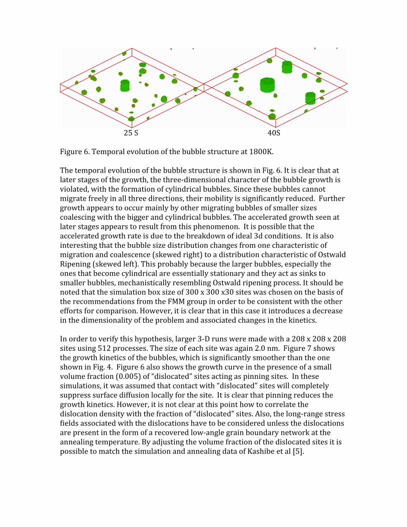
25S 40S

Figure6.Temporalevolutionofthebubblestructureat1800K.ThetemporalevolutionofthebubblestructureisshowninFig.6.Itisclearthatatlaterstagesofthegrowth,thethree‐dimensionalcharacterofthebubblegrowthisviolated,withtheformationofcylindricalbubbles.Sincethesebubblescannotmigratefreelyinallthreedirections,theirmobilityissignificantlyreduced.Furthergrowthappearstooccurmainlybyothermigratingbubblesofsmallersizescoalescingwiththebiggerandcylindricalbubbles.Theacceleratedgrowthseenatlaterstagesappearstoresultfromthisphenomenon.Itispossiblethattheacceleratedgrowthrateisduetothebreakdownofideal3dconditions.Itisalsointerestingthatthebubblesizedistributionchangesfromonecharacteristicofmigrationandcoalescence(skewedright)toadistributioncharacteristicofOstwaldRipening(skewedleft).Thisprobablybecausethelargerbubbles,especiallytheonesthatbecomecylindricalareessentiallystationaryandtheyactassinkstosmallerbubbles,mechanisticallyresemblingOstwaldripeningprocess.Itshouldbenotedthatthesimulationboxsizeof300x300x30siteswaschosenonthebasisoftherecommendationsfromtheFMMgroupinordertobeconsistentwiththeothereffortsforcomparison.However,itisclearthatinthiscaseitintroducesadecreaseinthedimensionalityoftheproblemandassociatedchangesinthekinetics.Inordertoverifythishypothesis,larger3‐Drunsweremadewitha208x208x208sitesusing512processes.Thesizeofeachsitewasagain2.0nm.Figure7showsthegrowthkineticsofthebubbles,whichissignificantlysmootherthantheoneshowninFig.4.Figure6alsoshowsthegrowthcurveinthepresenceofasmallvolumefraction(0.005)of“dislocated”sitesactingaspinningsites.Inthesesimulations,itwasassumedthatcontactwith“dislocated”siteswillcompletelysuppresssurfacediffusionlocallyforthesite.Itisclearthatpinningreducesthegrowthkinetics.However,itisnotclearatthispointhowtocorrelatethedislocationdensitywiththefractionof“dislocated”sites.Also,thelong‐rangestressfieldsassociatedwiththedislocationshavetobeconsideredunlessthedislocationsarepresentintheformofarecoveredlow‐anglegrainboundarynetworkattheannealingtemperature.ByadjustingthevolumefractionofthedislocatedsitesitispossibletomatchthesimulationandannealingdataofKashibeetal[5].

Fig.7.Bubblegrowthkineticsina416x416x416nm3simulationvolume

Fig.8.Bubblesizedistributionobtainedusing416x416x416nm3runFigure8showsthebubblesizedistributioninthecaseofthelargerrun.NotethatthetransitionfrommigrationandcoalescelikedistributiontoOstwaldRipeninglikedistributionseeninthesmallerrunnolongerexists.

5s 15s

30s 45s

Figure9showsthetemporalevolutionofthebubblesinthe416x416x416nm3runshowingmigrationandcoalescencemechanismoperatingthroughoutthesimulationtime.ThetemporalevolutionofthebubblesisshowninFig.9forthelargerrun.Itisclearthatthecylindricalbubblesthatformedinthesmallerdomaindonotformandthereisnosuddenincreaseinthegrowthrateasobservedinthesmallerrun.However,afewgrowthbumpsareseeninFig.7thatcorrespondstorarecoalescenceeventsassociatedwithlargebubbles.

ThecalibrationofthePotts/KMCcodecanberescaledatanytimeduringthesimulation,withtheassumptionthateachsimulationcellnowcorrespondstoalargerbubblesize.Thestructureshouldbere‐mappedsothatthespatialdistributionofthebubbleswillbepreserved.Withthisre‐mapping,itisnowpossibletochangetherelationshipbetweenMCSandtimesuchthateachMCSnowcorrespondstoalargerrealtime.Suchanapproachhasbeendemonstratedforsimulationgraingrowthinsteels[6].Thereforethesimulationscanbeusedefficientlytofollowthestructureevolutionatannealingtimesofhours.Input/DataNeeds

1. Effectivepinningforceduetodislocationsatanylocationduetothecumulativeeffectofallthedislocationswithinacutoffradius.Thisshouldalsotakeintoaccountwhetherthegeometryofthespatialdistributionofthedefects(tangleversusregularnetwork)

2. InterfacialenergyasafunctionoftemperatureandXenonpressure3. Strainandstraingradientinthematrixduetonon‐equilibriumbubbles

(whenbubblescoalesce)4. Kineticsofabsorptionofvacancyatthebubble‐matrixinterface.This

involvesmodelingthelong‐rangediffusionofvacanciesinthematrixinthepresenceofthedislocations

5. Attachment‐detachmentkineticsforvacanciesnearnon‐equilibriumbubblesBibliography

1. R.Montgomery,internalcommunication.2. T.Suzudoetal.,“Athree‐dimensionalmesoscalemodelingforbubblegrowth

inmetals,”ModellingSimul.Mater.Sci.Eng16(2008)0550033. C.Ronchi,“ExtrapolatedEquationofStateforrareGasesatHigh

TemperaturesandDensities,”JNM96(1981)314‐3284. T.G.Desaietal.,“AtomisticSimulationsofVoidMigrationunderThermal

GradientinUO2,”ActaMater.58(2010)330‐339.5. S.Kashibe,K.UneandK.Nogita,“FormationandGrowthofIntragranular

FissionGasBubblesinUO2FuelswithBurnupof6‐83GWd/t,”JNM206(1993)22‐34

6. B.RadhakrishnanandT.Zacharia,“MonteCarloSimulationofGrainBoundaryPinningintheWeldHeatAffectedZone,”MetallurgicalandMaterialsTransactionsA,26(1995)2123‐2130.

AppendixELANL‐‐DatafromAtomisticSimulationsDavidAnderssonLosAlamosNationalLaboratoryThissectioncontainsabriefdiscussionof themodelparametersthatarerequiredfor simulating UO2 post‐irradiation annealing experiments at the meso‐scale. Wefocus on perspectives obtained from recent atomic level simulations and relatethese results to available experiments. The discussion is not meant to cover allaspects of the problem, but rather exemplifies a few cases where atomic levelsimulationshavemadeanimpactontheunderstandingofmaterialpropertiesthatcouple directly to meso‐scale models. This work is published [1,2,3,4] or in theprocessofbeingpublished[5,6].OxygeninterstitialsandvacanciesFrom both simulations [2,3,5] and experiments [7,8,9] it is clear that oxygenvacanciesandinterstitialsmoveseveralordersofmagnitudefasterthroughtheUO2latticethancationsorfissiongases.Themigrationbarriersforanionvacanciesandinterstitialsare0.5[7,10]and0.9‐1.3eV[6,7,10],respectively,while the lowestbarrier for cations (a cluster of two uranium vacancies that can form underirradiation) is predicted to be 2.6 eV [3] and the barrier for migration of singleuranium vacancies is 4.5‐4.8 eV [3,5]. Based on these observations it isrecommendedtomakesimplifyingassumptionsregardingthedistributionofaniondefects,sincefullcouplingofcationandaniondynamicswouldresultinsignificantnumerical challenges. One possibility is to treat anion species as always being inequilibriumwithrespecttothedistributionofcationdefects.ForstoichiometricUO2where oxygen vacancies and interstitials appear in approximately equalconcentrations under thermal equilibrium, transport occurs predominantly viavacancies due to their lower migration barrier. For UO2+x the concentration ofoxygen interstitials or clusters thereof exceeds that of vacancies. Consequently,interstitials and clusters of interstitials dominate the diffusion properties in thisstoichiometry range [2,6,11]. In addition to the kinetic properties, meso‐scalemodels need information regarding the concentration of oxygen vacancies andinterstitials. This is available from thermodynamic models derived from eitherexperiments [12] or from calculations [1,3]. For strictly stoichiometric UO2 theoxygenvacancyformationenergyandtheinterstitialformationenergyarebothhalftheFrenkelenergy,whichimplies1.5‐2.0eVfromboththeory[3]andexperiments[8,9].UraniuminterstitialsandvacanciesMigrationofuraniuminterstitialswasrecentlyinvestigatedusingdensityfunctionaltheorycalculations[5]andthebarrierwascalculatedtobe3.7eVfor the indirect

interstitialcy mechanism, which is lower than the barrier for single uraniumvacanciesbutabout1eVhigherthanforclustersofuraniumvacancies(seebelow).Under thermal equilibriumconditions the contribution from interstitials to cationdiffusionisverysmallduetothenegligibleconcentrationofsuchdefectscomparedto vacancies [5]. The activation energy for the uranium interstitialcy diffusionmechanisminstoichiometricUO2wascalculatedtobeashighas15‐16eV[5].Experiments typicallyquote2.4eVas themigrationbarrierofuranium ionsviaavacancy mechanism [8,9], which was derived by studying the recovery of UO2samples exposed to irradiation. If non‐equilibrium clusters form under suchconditionsthemeasuredbarriercouldreferto, .e.g.,migrationofuraniumvacancyclustersratherthanisolatedvacancies.Thiswasconfirmedbyrecentcomputationalstudies,whichpredictedabarrierofabout4.5‐4.8eVforsingleuraniumvacanciesandabout2.6eVfortwonearestneighboruraniumvacancies[3].Simulationsofin‐pile conditions should probably apply the lower cluster barrier, while the higherbarrier for single uranium vacancies may better describe out‐of‐pile conditions.Uraniumdiffusion under thermal equilibrium conditions has beenmeasured by anumber of authors [8,9,13]. For stoichimetric UO2 the corresponding activationenergyisreportedtorangefrom4.4[13]to5.6eV[8,9].Theactivationenergyisastrong functionof theUO2x stoichiometry.ForUO2‐xandUO2+x the correspondingactivationenergieswerereportedtobe7.8and2.6eV,respectively. InRef.[3]weuseddensity functional theorycalculationsto investigatetheactivationenergy foruranium diffusion. Even though the agreement between theory and experimentswasrathergood[3],themodelusedforcalculatingtheactivationenergiesfromthecalculated thermodynamic and kinetic data was incomplete. A second paper [5]explored this in more detail for stoichiometric UO2 and we achieved improvedagreementwithexperimentscomparedtotheearlierstudy[5].Themostuptodateactivation energy foruraniumdiffusion inUO2 is 4.4eV [13] andour calculationspredict4.1‐4.9eV[5].Whetherthemeso‐scalesimulationsshouldusethecalculatedmigration barrier or the activation energy to describe the Arrhenius rates in thetransport equations depends on the conditions that are being simulated, e.g.irradiation environments or thermal concentration of defects, and how thedeviationfromthermodynamicequilibriumisformulated.Theeffectivevalueoftheuranium vacancy formation energy depends on stoichioemtry and chemicalenvironment.ForstrictlystoichiometricUO2wesuggest2.69eV[3].FissiongasIn order to understand fission gas transport one must first determine how theatomsinteractwiththefluoriteUO2host,bothwhatisthemoststableequilibriumtrap site but also high energy positions that might result as a consequence ofirradiation,andthesubsequenttransportmechanismsforallformsofthegaswithinthematrix.Amongthefissiongases,Xeisthemostprominent.MiekeleyandFelix[14] performed early experiments on the release of Xe during post‐irradiationdiffusion anneal fromUO2±xwith a range of different stoichiometries (x). Perhapsthemost striking conclusion from theirworkwas that the activation energies forreleaseexhibiteduniquevaluesintheUO2‐x(6.0eV),UO2(3.9eV)andUO2+x(1.7eV)

regimes, respectively, while they were almost constant within each of thesecompositionsets.ThiswasinterpretedasXeatomsoccupyingvacancytrapsites,aconcept that was investigated by Catlow [16] using empirical potentials of theBuckingham type. Later Ball et al. [15] applied similar techniques to investigatestabilityofXeintrapsitesasfunctionofstoichiometryandchargestate.AccordingtoBalletal.[15],XeatomseitherresideinaneutraltrivacancyclusterforUO2‐xandUO2,adivacancyforUO2orinaUvacancyforUO2+x.TheseconclusionsagreewellwithearlierresultsbyCatlow[16]andalsobymorerecentDFTwork[19].TheXesolutionthermodynamicsestablishesthefoundationforspeciestransport,andBalletal.[15,17]furtherinvestigatedhowtheXeatomsmaymovefromonelatticesitetoanotherbybindingasecondUvacancytotherespectiveXetrapsites–avacancymediateddiffusionmechanism. TheyproposedthatXetransportoccursbytheXeatom jumping from its original trap site to the second bound vacancy, whichconstitutesthecenterofanewXetrapsiteafterthismigrationstep.InorderfornetXetransporttotakeplace,motionofthesecondvacancyboundtotheXetrapsitemustbeconsidered.SinceBalletal.didnotattempttostudythelatterstep,theydidnotcomparetheircalculateddatawithmeasuredactivationenergies.We applied the DFT+U methodology to study diffusion of Xe under a variety ofconditions [3]; inparticularapplying the thermodynamicmodeloriginallyderivedby Catlow [16] to calculate activation energies for Xe in theUO2‐x, UO2 andUO2+xranges.ThistransportmodelrequirescalculationofthebindingenergyofasecondUvacancy to theXe trap site and thebarrier formovingoneof the constituentUvacancies to another location such that net transport is enabled. This diffusionmechanisminvolvesthreecomponents:theVUformationenergy,thebindingenergyof this vacancy to the Xe trap site, and the intra‐clustermigration barrier for theindividualUvacanciesboundtothiscluster.Thatis,therate‐limitingstepisnotXemotion within the cluster, but the migration of the second vacancy within thecluster;withoutthemotionofthesecondboundUvacancyXedoesnotdiffuse.We note that many earlier studies dismissed vacancy mechanisms, which wasmotivated by a number of experimental observations summarized by Matzke [9]andMiekeleyandFelix[14].Forexample,theactivationenergyintheUO2+xregimewas found to be a constant and it did not changewith stoichiometry. However,accordingtoourunderstanding,inexperimentswherethecompositionisallowedtovaryasfunctionoftemperatureaccordingtothermodynamicequilibriumrelations,the Xe activation energy should contain an additional term coming from thetemperature dependence of the stoichiometry. Miekeley and Felix [14] estimatedthecorrespondingArrheniusenergytobe‐0.3eVforUO2andUO2+xbasedontheirexperiments. According to the thermodynamicmodel derived by Catlow [16] forUO2+xweshouldaddtwicethisenergytotheXeactivationenergyifthecompositionisnotkeptfixedintheexperiments.Thiscontributionwasnotaccountedforinanycomputationalstudiessofar,butaddingthistermtothecalculatedvaluesfortheXeactivation energy in the UO2+x range in fact improves the agreement with theexperimentaldataofMiekeleyandFelix[14].Preliminaryworkindicatesthatwhentheappropriatethermodynamicmodelsareappliedtheactivationenergiesderived

fromdensityfunctionaltheorycalculationsareveryclosetothevaluesmeasuredbyMiekeleyandFelix[14]forallstoichiometries.Moreover,Govers[18]showedthatalternative mechanisms based on migration via interstitial sites are unfavorable,thuslendingsupportforthevacancymechanism.ThebarriersformovingoneoftheuraniumvacanciesfromonepartoftheXetrapsitetoanotheris3.91,5.00and5.51eVfortheXeU(Xeoccupiesoneuraniumvacancy),XeUO(Xeoccupiesoneuraniumand one oxygen vacancy) and XeUO2 (Xe occupies one uranium vacancy and twooxygen vacancies) trap sites, respectively. The corresponding defect formationenergiesarelistedinRef.[3].ForstrictlystoichiometricUO2wesuggest4.35eV.Fissiongasescanalsodiffuseviainterstitialmechanisms.DuetothelargesizeofXeatoms it is however unlikely that such mechanisms are important at hightemperaturesincetheinterstitialXeatomswouldquicklyrecombinewithuraniumvacancies. If theXeatomstays in interstitialpositions itmaydiffusewitharatherlowbarrier(1.6eV)comparedtovacancymechanisms[4].DefectformationvolumesTable1liststheformationvolumesofoxygen,uraniumandfissiongas(Xe)defectsin stoichiometric UO2. Theywere all calculated according to the definition of thecorresponding defect formation energies [3]. Note that this definition is slightlymorecomplexthanin,e.g.,puremetals,whichmustbeaccountedforinthemeso‐scalemodels.Table 1: Formation volume of defects in stoichiometric UO2.

Defecttype Formationvolume[Å3]Oxygenvacancy 1.79Oxygeninterstitial 1.79Uraniumvacancy 42.3Schottkydefect(unbound) 45.8Schottkydefect(bound) 41.9Xe 52.8References1.D.A.Andersson,J.Lezama,B.P.UberuagaandS.D.Conradson,Phys.Rev.B79,024110(2009).2. D. A. Andersson, T. Watanabe, C. Deo, and B. P. Uberuaga, Phys. Rev. B 80,060101(R)(2009).3.D.A.Andersson,B.P.Uberuaga,P.V.Nerikar,C.Unal,andC.R.Stanek,Phys.Rev.B84,054105(2011).4. X.‐Y.Liu,B. P.Uberuaga,D.A.Andersson, C.R. Stanek, andK.E. Sickafus,Appl.Phys.Lett.98,151902(2011).5.BorisDorado,DavidA.Andersson,ChristopherR.Stanek,MarjorieBertolus,BlasP. Uberuaga, Guillaume Martin, Michel Freyss and Philippe Garcia, submitted forpublication.6. D. A. Andersson, F. J. Espinosa‐Faller, B. P. Uberuaga and S. D. Conradson,submittedforpublication.

7. G. E.Murch andC. RichardA. Catlow, J. Chem. Soc., FaradayTrans. 283, 1157(1987).8.Hj.Matzke,J.Chem.Soc.,FaradayTrans.283,1121(1987).9.Hj.Matzke,Radiat.Eff.Defect.S.53,219(1980).10. B. Dorado, P. Garcia, G. Carlot, C. Davoisne, M. Fraczkiewicz, B. Pasquet, M.Freyss,C.Valot,G.Baldinozzi,D.SimeoneandM.Bertolus,Phys.Rev.B83,035126(2011).11.P.RuelloandG.ChirlesanandG.Petot‐ErvasandC.PetotandL.Desgranges, J.Nucl.Mater.325,202(2004).12.C.Gueneau,M.Baichi,D.Labroche,C.ChatillonandB.Sundman,J.Nucl.Mater.304,161(2002).13.A.C.S.Sabioni,W.B.FerrazandF.Millot,J.Nucl.Mater.257,180(1998).14.W.MiekeleyandF.W.Felix,J.Nucl.Mater.42,297(1972).15.R.G.J.BallandR.W.Grimes,Chem.Soc.,FaradayTrans.86,1257(1990).16.C.R.ACatlow,Proc.R.Soc.LondonSer.A364,473(1978).17.R.G.J.BallandR.W.Grimes,J.Nucl.Mater.188,216(1992).18.K.Govers,S.E.LemehovandM.Verwerft,J.Nucl.Mater.405,252(2010).19.P.V.Nerikar,X.‐Y.Liu,B.P.Uberuaga,C.R.Stanek,S.R.PhillpotandS.B.Sinnott,J.Phys.‐Condens.Mat.21,435602(2009).

Mesoscale Benchmark Demonstration - Pacific … · Mesoscale Benchmark Demonstration ... and Oak...

Documents

Transcript of Mesoscale Benchmark Demonstration - Pacific … · Mesoscale Benchmark Demonstration ... and Oak...