INTRASITE SPATIAL ANALYSIS AND INTERPRETATION OF MAPPED

SURFACE ARTIFACTS IN CA-SNI-25, SAN NICOLAS ISLAND, CALIFORNIA

A Thesis

Presented to

The Faculty of the Department of Anthropology

California State University, Los Angeles

In Partial Fulfillment

of the Requirements for the Degree

Master of Arts

By

Michael L. Merrill

June 2004

ACKNOWLEGEMENTS

This project required the assistance and support of several people as well as the

United States Navy. I want to thank Dr. Patricia Martz for suggesting this project to me

and for providing needed encouragement and advice throughout its duration. I could not

have asked for a better mentor at Cal State LA or anywhere for that matter than Dr.

Martz. I will forever appreciate the knowledge you shared and for the doors of

opportunity opened for me, Dr. Martz. I am also thankful for the excellent field assistance

and professional site evaluation provided by Dan Larson and John Romani of Compass

Rose Archaeological Inc. during the initial data collection phase of this project. I would

also like to acknowledge the following Cal State LA students, listed in alphabetical order,

for their excellent and dedicated assistance with the mapping and recordation of surface

artifact positions and types at CA-SNI-25: Charles Cisneros, Lina Flores, Catherine

Girod, Walter Henriguez, Emilio Merino, and Vicki Stossel. I also extend thanks to Rod

McLean for his outstanding and patient instruction, both in the classroom and the field, in

using the theodolite on one visit to San Nicolas Island. This was during the latter

recordation phase of this project. Walter and Emilio also received instruction from Rod

on this visit and assisted in using a theodolite and stadia rod at CA-SNI-25 to set up a site

grid and boundary. Thank you again, Rod, Walter, and Emilio for your sincere and

excellent help. I also am indebted to Steve Schwartz for making this project possible by

providing the financial and logistical support. Thank you Steve for your help and for

sharing some of your knowledge and ideas concerning the prehistory of San

Nicolas Island. I found several of these ideas very insightful, especially the importance of

driftwood to the native people of San Nicolas Island. I would also like to extend my

gratitude and appreciation to the United States Navy for allowing me to conduct research

on San Nicolas Island.

I want to express a deep and heartfelt appreciation to the members of my thesis

committee, Patricia Martz, Ph.D. (Chair), Chester King, Ph.D., James Brady, Ph.D., and

Dwight Read, Ph.D. Patricia Martz, Chester King, and James Brady carefully read the

archaeological sections of my thesis. They provided editorial, logical, and factual

corrections that significantly improved the accuracy and quality of presentation of the

archaeological, ethnographic, and empirical data contained in this thesis. Professor

Dwight Read of UCLA critically reviewed the applied mathematics in my thesis. His

suggestions and corrections significantly improved the quality and presentation of the

statistical and mathematical methods. Dr. Read is currently assisting me in preparing

some of my research work for publication. I plan on continuing my studies in

archaeology at UCLA with the sponsorship of Dr. Read.

Finally, I want to give special thanks to my friend and long time mentor in

archaeology, Dr. Chester King. Chester is a scientist who possesses the rare combination

of remarkable ability, consummate skill, and a genuine concern and respect for the people

and cultures he studies. Without Chester’s friendship, guidance, and encouragement I

would not have become an archaeologist. Thank you Chester.

ABSTRACT

An Intrasite Spatial Analysis and Interpretation of Mapped Surface Artifacts at CA-SNI-

25, San Nicolas Island, California

By

Michael L. Merrill

The focus of this research project is the objectification of the internal organization

in CA-SNI-25, a Late period village site overlooking the northwest coastline of San

Nicolas Island, one of the Southern Channel Islands off the coast of Southern California.

There is a major gap in knowledge pertaining to the internal organization of village sites

on this island. To address this gap, mathematical analyses of typed surface artifact

distributions in CA-SNI-25 as well as provenience-based counts of typed artifacts from

an excavation in a coastal Chumash village site (CA-VEN-27) of similar occupation span

were performed. Archaeological, experimental, ethnographic, and ethnohistoric

information were used to interpret these analyses. Specifically, the location and artifact

composition of areas of organized activity as well as tool kits were inferred by the

analyses of the CA-SNI-25 data. The analysis of the CA-VEN-27 or Pitas Point data was

used to discover tool kits. The Pitas Point data are a more complete sample than the

sample from CA-SNI-25. For this reason the results of the analysis of the Pitas Point data

were used as a predictive model for associations of artifact types not present in the CA-

SNI-25 sample but present in the site.

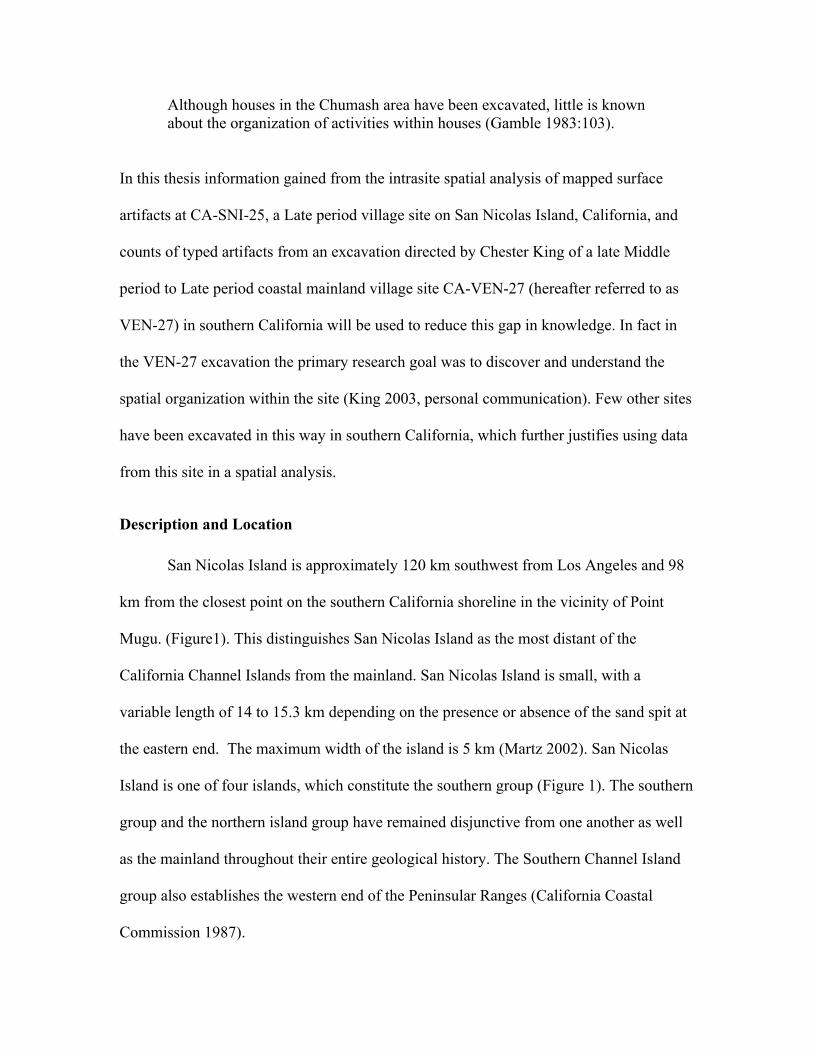
In addition, other archaeological data such as CA-SNI-11 tarring pebble data are

used in this thesis to buttress the interpretations of the Pitas Point analysis as well as the

results of the analyses of the CA-SNI-25 data.

Surface artifact clusters that are interpreted as four house locations were

discovered in the sampling area of SNI-25, using a nearest neighbor analysis. Each of

these clusters has mortar fragments and core tools such as chopper/hammers.

Ethnography supports interpreting these four artifact clusters as house locations. The

three northern house locations (House Activity Areas #1, #2, and #3) are tightly clustered

at the north edge of the site. The close proximity of these house activity areas to one

another suggests they are contemporaneous. The southernmost house location (House

Activity Area #4) is disjunct (about fifteen meters south) from the northern “house”

cluster. This significant spatial separation may result from House Activity Area #4 being

part of a separate and possibly non-contemporaneous house cluster.

Two additional surface artifact clusters in the SNI-25 sampling area were

identified with the nearest neighbor analysis. These two artifact clusters are interpreted as

outdoor activity areas based primarily on the absence of mortars and pestles (household

kitchen tools) and the presence of large clusters of metavolcanic and quartzite flakes and

retouched flake tools such as scrapers and blades. The northernmost of these two clusters

(Outdoor Activity Area #1) is intermediate between House Activity Area #3 and House

Activity Area #4. It is likely that this activity area is connected to both House Activity

Area #3 and #4, but could have been used at two disparate time periods if the occupations

of House Activity Area #3 and #4 do not temporally overlap. The southernmost cluster

(Outdoor Activity Area #2) is juxtaposed and to the east of House Activity Area #4. This

outdoor activity area is almost certainly tied to this house activity area alone.

The types of activities inferred by clusters of surface artifacts (activity loci) within

the four household areas and in areas immediately next to these areas are as follows: (1)

Food processing and cooking (inferred by fire-affected rock) and (2) Wood, bone, and

shell working. The types of activities inferred by clusters (activity loci) of surface

artifacts within the two outdoor activity areas are as follows: (1) Butchering and (2)

Wood, bone, and shell working,

Two additional mathematical analyses were used to discover tool kits in CA-

VEN-27 and CA-SNI-25. Both of these analyses use methodology that is entirely original

and applied to archaeological data for the first time in this thesis. The first analysis is a

synthesis of Pearson correlation analysis and graph theory and used typed artifact counts

from four excavated areas in CA-VEN-27 as raw data. Four tool kits were discovered

with this analysis. The second analysis combines a robust and distribution-free non-

parametric statistical method, known as a multi-response permutation procedure (MRPP),

and Graph Theory. This analysis used the point provenience of typed surface artifacts in

the sampling area of CA-SNI-25 as raw data. Three tool kits were discovered with this

analysis. The tool kits identified by these analyses together with the results of an analysis

of CA-SNI-11 tarring pebbles, along with ethnography and information from replicative

experiments and micro-wear analysis on stone tools (Keeley, 1980) suggest additional

types of activities at both CA-SNI-25 and CA-VEN-27. These activities include

groundstone production and the manufacture of several types of basketry (e.g. “water

bottles”).

TABLE OF CONTENTS

Acknowledgements………………………………………………………………………iii

Abstract…………………………………………………………………………………...vi

List of Tables………………………………………………………………………….…..x

List of Figures………………………………………………………...……...…………..xii

List of Tables

Table 1. Excel 4.0 macro…………….……………….…………………….……………25 Table 2. Various probabilities of incorrectly rejecting or correctly rejecting the null hypothesis for a given number of iterations……………………………….……………..26 Table 3. Details of the computation of an exact multi-response permutation procedure delta for the observed hypothetical distribution of scrapers and choppers in Figure 10……………………………………………………………………………….……...…36 Table 4. Exact multi-response permutation procedure delta values and corresponding P-values for each of fifteen possible two- four combinations of hypothetical surface artifact locations…………………………………………………………………..……………...37 Table 5. Statistically significant results of the nearest neighbor analysis applied to mapped surface artifacts in the sampling area in CA-SNI-25……………..…………….48 Table 6. Typed artifact counts from four excavated areas in CA-VEN-27………...…....63 Table 7. Pearson correlation coefficient matrix computed from the CA-VEN-27 typed artifact counts in Table 6……………………………………………………..…………..64 Table 8. Adjacency matrix resulting from the binary coding of the correlation coefficient matrix in Table 7 using a cut-off of 0.78………………..……………...........65 Table 9. Cliques resulting from a cut-off of 0.77 in the correlation matrix (Table 7)………………………………………………………………………………………....67 Table 10. Cliques resulting from a cut-off of 0.78 in the correlation matrix (Table 7)………………………………………………………………………………….……...67

Table 11 Cliques resulting from a cut-off of 0.79 in the correlation matrix (Table 7)…………………………………………………………………………………………67 Table 12. Resulting cliques that are interpreted as either house or outdoor activity area tool kits in CA-VEN-27…………………………………………………………….....…69 Table 13. The format used to enter the mass data for CA-SNI-11 tarring pebble samples into the Blossom statistical software…………………………………………………..…79 Table 14. Radiocarbon dates from two units in Mound B of CA-SNI-11……………….79 Table 15. Exact Multi-response Permutation Procedure delta P-values for each of the pairs of tarring pebble samples from CA-SNI-11…………………………...…………...81 Table 16. CA-SNI-25 surface artifact types used in the exact multi-response permutation procedures………………………………………………………………….88 Table 17. Delta P-value matrix constructed using the results of the Exact multi- response Permutation Procedures used for the pair-wise comparison of the spatial distribution of nine surface artifact types in the sampling area of CA-SNI-25….....................................88 Table 18. Adjacency matrix resulting from the binary coding of the exact multi- response permutation procedure

!

" P-values in Table 17 using a cut-off of 0.05……...…89 Table 19. Cliques resulting from a network analysis using the adjacency matrix in Table 18 as raw data……………………………………………………...………..…….89 Table 20. Adapted from Keeley (1980:112). Relationship between use and flake length resulting from experiments using replicated flakes…………………………….………..93 Table 21. ASCII format entered into the Blossom software to test for equality of medians of the data in Table 20, using Multi-response Permutation Procedures (MRPP) with absolute deviations (Euclidean Distance)………………..……........................................93 Table 22. Refer to description in thesis………………………………...…….………….94 Table 23. Results of the MRPP performed on the data in Table 20……………………..94

List of Figures

Figure 1. Channel Islands of Southern California………………………….………….….4 Figure 2. CA-SNI-25 Topographic Map…………………………………………………..8

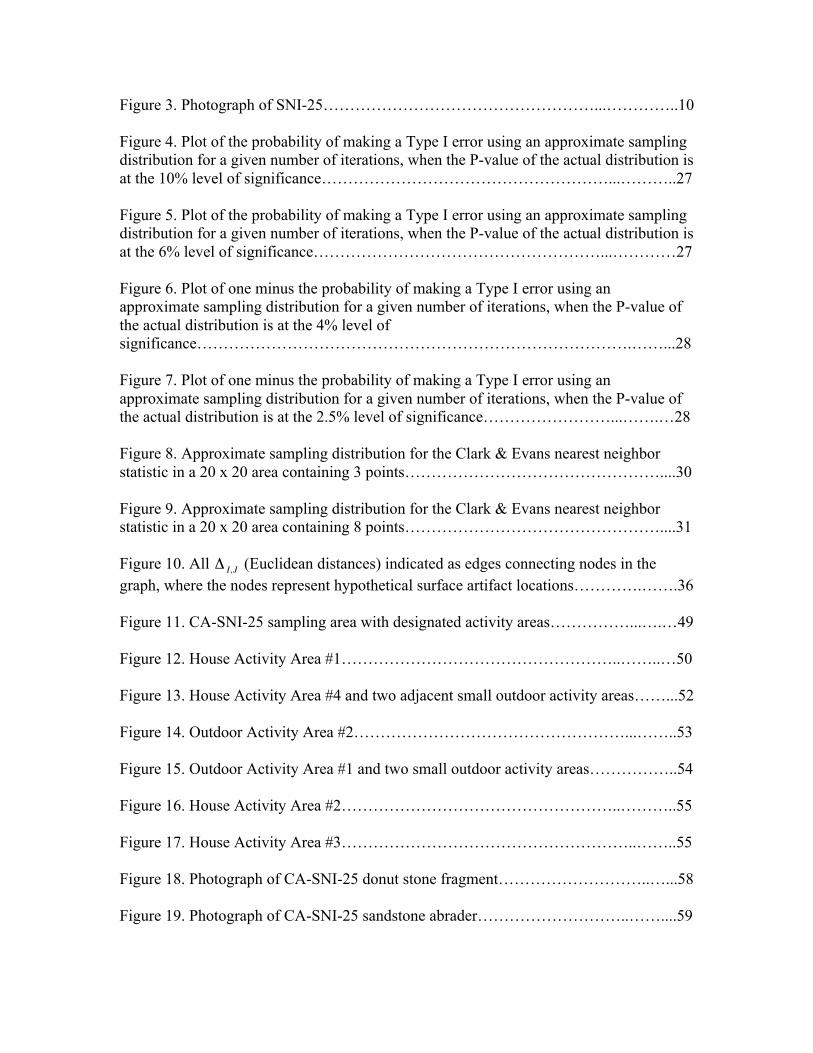
Figure 3. Photograph of SNI-25……………………………………………...…………..10 Figure 4. Plot of the probability of making a Type I error using an approximate sampling distribution for a given number of iterations, when the P-value of the actual distribution is at the 10% level of significance………………………………………………...………..27 Figure 5. Plot of the probability of making a Type I error using an approximate sampling distribution for a given number of iterations, when the P-value of the actual distribution is at the 6% level of significance………………………………………………...…………27 Figure 6. Plot of one minus the probability of making a Type I error using an approximate sampling distribution for a given number of iterations, when the P-value of the actual distribution is at the 4% level of significance……………………………………………………………………….……...28 Figure 7. Plot of one minus the probability of making a Type I error using an approximate sampling distribution for a given number of iterations, when the P-value of the actual distribution is at the 2.5% level of significance……………………...…….…28 Figure 8. Approximate sampling distribution for the Clark & Evans nearest neighbor statistic in a 20 x 20 area containing 3 points…………………………………………....30 Figure 9. Approximate sampling distribution for the Clark & Evans nearest neighbor statistic in a 20 x 20 area containing 8 points…………………………………………....31 Figure 10. All

!

" I,J (Euclidean distances) indicated as edges connecting nodes in the graph, where the nodes represent hypothetical surface artifact locations………….…….36 Figure 11. CA-SNI-25 sampling area with designated activity areas……………...….…49 Figure 12. House Activity Area #1……………………………………………..……..…50 Figure 13. House Activity Area #4 and two adjacent small outdoor activity areas……...52 Figure 14. Outdoor Activity Area #2……………………………………………...……..53 Figure 15. Outdoor Activity Area #1 and two small outdoor activity areas……………..54 Figure 16. House Activity Area #2……………………………………………..………..55 Figure 17. House Activity Area #3………………………………………………..……..55 Figure 18. Photograph of CA-SNI-25 donut stone fragment………………………..…...58 Figure 19. Photograph of CA-SNI-25 sandstone abrader………………………..……....59

Figure 20. Plot of the frequencies of the correlation coefficients from Table 7………....66 Figure 21. CA-VEN-27 Artifact Association Network Graph…………………….…….70 Figure 22. Tarring pebble maximum length verses mass scatter plot and linear regression…………...………………………………………………………….………...81 Figure 23. Plot of the mass of two samples of tarring pebbles from CA-SNI-11…...…...82 Figure 24. Plot of the mass of a sample of small and large tarring pebbles from CA-SNI-11…………………………………………………………………………………….…...82 Figure 25. Plot of the mass of a second sample of small and large tarring pebbles from CA_SNI-11………………………………………………………………………..……..83 Figure 26. Plot of the mass of a third sample of small and large tarring pebbles from CA-SNI-11…………………………………………………...……………………………….83 Figure 27. Plot of the mass of a fourth sample of small and large tarring pebbles from CA-SNI-11………………………………………………………………………..……...84 Figure 28. Photographs of a small water bottle and tarring pebbles…………………..…86 Figure 29. CA-SNI-25 Artifact Association Network Graph………………….……...…90 Figure 30. Plot of the flake length frequencies corresponding to two activity types for each of the six length classes in Table 13……………………………………….……….95 Figure 31. Relative frequency plot of metavolcanic flake length from a sample taken in an outdoor activity area in the CA-SNI-25 sampling area……………...…...….97 Figure 32. Relative frequency plot of quartzite flake length from a sample taken in an outdoor activity area in the CA-SNI-25 sampling area……………………………..…...97 Figure 33. Relative frequency plot of metavolcanic flake length from a sample taken in a house activity area in the CA-SNI-25 sampling area………………………..……..102 Figure 34. Relative frequency plot of quartzite flake length from a sample taken in a house activity area in the CA-SNI-25 sampling area…………………….………..……102 Figure 35. Theoretical energy flow and storage model of a possible subsystem in CA-SNI-25……………………………………………………………….………………….112

Chapter 1. Introduction…………………………………………..………………………...…...……..1 Importance of Studying Internal Site Structure…………………………..……..……...1

Description and Location……………..…………...……………………....…...….……2

Geology, Topography, and Environmental Setting………...………….………......…...3 CA-SNI-25……….…………………………………………………………….…...…..7 Overall Aims and Potential Contribution to Future Research……………...……....…..9 Background and Significance…………………………….………….…….....…….…12 Research Goals…………………………...….…….………………..…..…….……….13 Importance of this Research………………………………......……………....……….13 Pre and Post Depositional Disturbance……………………………..……....….......….14 Research Questions and Hypotheses…………………………..…...……………....…15 2. Methodology………………………………….…………………….……………...….18

Sampling Procedure………………………………………………..……………….…18

The Applied Mathematical Methods Used in this Study……..………….……………19 The Clark & Evans Nearest Neighbor Statistic and its Previous Use in Archaeology…………………………………………………………….……………..20

A Monte Carlo Test of Spatial Randomness……………….………....…….……..…..21

Calculating Probability p from an Approximate Sampling Distribution……………...29 Discovering Features Within a Site……………..……….…..………..…....…………29

Correlation Analysis……………………..………………..…..…...……..…………...31

Exact Multi-Response Permutation Procedures (EMRPP)………...………….………33 Graph Theory and Network Analysis……………..…………..…………………..…..35

3. Intrasite Spatial Analysis……………………………………...….…………………...43 Definition of Activity Area…………………………...…………............…...………..43

Dichotomy of House and Outdoor Activity Areas……………………………..……..43 Criteria for Identifying House and Outdoor Activity Areas………………...….……..44 Locations of House and Outdoor Activity Areas in the Sampling Area of CA- SNI-25………...………………….…………………..…………………....……….….47 Interpretation of Results…………...……...…………………..…………………..…...48 Tool Kits and Activity Areas in the Pitas Point Site, CA-VEN-27………..........….....57 Methods of Analysis……......…………...………………..…….….…….…...……….61 The Network Graph of Artifact Types in CA-VEN-27………...………….………….68 Interpretation of Results…………….....…..…………….……………….......………..71 Tool Kits and Activity Areas in CA-SNI-25…….……….……….……..…...…...…..87 Methods of Analysis….....…………………...…………………...……….......………87 Interpretation of Results……………..…………...…………………….……..…..…...90 Comparison of Tool Kits in CA-VEN-27 and CA-SNI-25…………….......…….….103 Conclusion…………..………..………………………………………….…..………104 4. Summary, Conclusions, and Recommendations for Future Research……………….109 Summary and Conclusions……………….…..…………...…………………..……..109 Recommendations for Future Research……………….…….……..…….…………..109 References Cited….…………...……………….…………...…………...…….………..114 Appendices……………………………………………………………....……………...123 A. Excel 4.0 Macros……………………………………………..…………..……….123 B. CA-SNI-25 Artifact Types and Locations…………….….……………...……….126 C. CA-SNI-25 Flake Length Tables...……………...…………..………...………….130

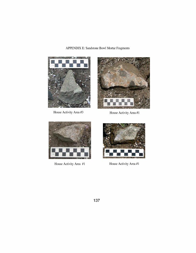
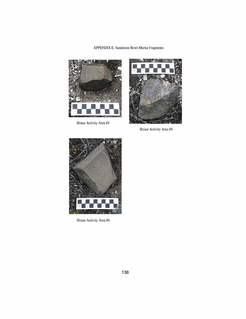
D. CA-SNI-11 Tarring Pebble Data Table...….………...……………….…………..131 E. CA-SNI-25 Artifact Pictures…………………..……………………....………….132

CHAPTER 1

INTRODUCTION

Importance of Studying Internal Site Structure

The spatial distribution of cultural materials within an archaeological site results

to a large degree from past human activity. It can be postulated that the various types of

activities that occurred within an archaeological site are the dynamic components or

subsystems of a larger social system. In considering the nature of a social system Harary

and Batell (1981) introduce a general graph-theoretic model that is applicable to any

hierarchical system. In this model a social system can be formally defined as a nested

social network whose underlying structure is a nested graph. The components of the

underlying structure clearly are the various subsystems that collectively compose the

structure of the entire system, which in turn influences the structure of the various

subsystems. All considered it is expected that the traces of past human activity within an

archaeological site when viewed as the remnants of specific social subsystems must be

recurrent and have identifiable structure. Therefore, discovering the internal structure of

an archaeological site is a necessary step toward understanding how the entire social

system of a particular prehistoric society functioned and was maintained.

There is a major gap in knowledge concerning the organization of activities

within prehistoric archaeological sites in coastal southern California.

Gamble comments on this deficit of knowledge of prehistoric site organization in coastal

southern California.

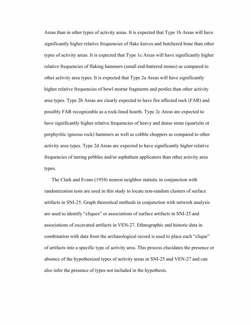
Although houses in the Chumash area have been excavated, little is known about the organization of activities within houses (Gamble 1983:103).

In this thesis information gained from the intrasite spatial analysis of mapped surface

artifacts at CA-SNI-25, a Late period village site on San Nicolas Island, California, and

counts of typed artifacts from an excavation directed by Chester King of a late Middle

period to Late period coastal mainland village site CA-VEN-27 (hereafter referred to as

VEN-27) in southern California will be used to reduce this gap in knowledge. In fact in

the VEN-27 excavation the primary research goal was to discover and understand the

spatial organization within the site (King 2003, personal communication). Few other sites

have been excavated in this way in southern California, which further justifies using data

from this site in a spatial analysis.

Description and Location

San Nicolas Island is approximately 120 km southwest from Los Angeles and 98

km from the closest point on the southern California shoreline in the vicinity of Point

Mugu. (Figure1). This distinguishes San Nicolas Island as the most distant of the

California Channel Islands from the mainland. San Nicolas Island is small, with a

variable length of 14 to 15.3 km depending on the presence or absence of the sand spit at

the eastern end. The maximum width of the island is 5 km (Martz 2002). San Nicolas

Island is one of four islands, which constitute the southern group (Figure 1). The southern

group and the northern island group have remained disjunctive from one another as well

as the mainland throughout their entire geological history. The Southern Channel Island

group also establishes the western end of the Peninsular Ranges (California Coastal

Commission 1987).

Geology, Topography, and Environmental Setting The geology of San Nicolas Island has been described as “a faulted asymmetric

anticline composed of Pleistocene sediments lying unconformably on Eocene sandstone

and shale (Meighan and Eberhart 1953:109). Erosion has resulted in the formation of 11

recognized terraces (Vedder and Norris 1963). San Nicolas Island is 276 meters at it

highest point and is mostly unprotected from frequent and strong northwesterly winds,

which average 25 km per hour. The low-lying topography of the island also contributes to

a very low average annual precipitation of 17.8 cm. This results in a xeric terrestrial

environment, which in the absence of fog drip would be classifiable as a desert on the

basis of less than 25.4 cm of rainfall in an average year.

Reinman and Lauter (1984) divided the island into three zones: (1) northern

coastal terrace; (2) southeast coastal terrace; and (3) central plateau (above the 400-foot

contour).

The plateau is characterized by being open and flat, and by the presence of

stabilized dunes. This area also contains eroded dunes, sand and sandy loam soils, cobble

outcrops, and deflated areas of caliche.

Eroded cliffs and dry canyons surround the plateau and drop abruptly to the sea. The

shoreline of the island is mostly rocky intertidal, though sandy beaches, dunes, and

coastal flats are also present. Fresh water on the island exists as springs, seeps, water

catchments, and an intermittently perennial watercourse, Tule Creek (Martz 2002).

The native flora of San Nicolas Island consists primarily of decumbent and low

growing herbaceous perennial shrubs along with annual and biennial flowers and grasses.

Trees with the possible exception of Salix lasiolepis (arroyo willow) are not native to this

island (Foreman 1967). Coreopsis gigantea and a common low growing lupine are

keystone perennials in the dune and coastal strand plant communities of the island. Two

native plants may have been managed as crops on the island. The small bulb

Dichelostemma capitatum (blue dicks) is well adapted to the harsh environment of San

Nicolas Island and is locally abundant on the plateau in the spring. This diminutive

member of the lily family may have been managed as a crop by the native inhabitants and

was undoubtedly an important food plant. Bulbs of this plant were likely roasted in earth

ovens and stored in baskets and pits (King 2002). The small annual flower Calandrinia

ciliata (red maids) blooms on the island during the spring. Seeds of this annual are known

to have been an important food source in coastal southern California and it has been

hypothesized that red maids were managed as a crop (King 2002). The fruit and pads of

the prickly pear cactus Opuntia littoralis were also predictably an important crop on San

Nicolas Island and the seasonal fruit was likely stored in baskets and/or pits as a rich and

long-term source of carbohydrates. The pads of prickly pear cactus were also likely used

for an unobvious purpose on San Nicolas Island, namely as fish bait. Fages (1775)

provides an ethnohistoric description of the use of cactus in sardine (Sardinops sagax

caeruleus) fishing by the Chumash of southern California.

For catching sardines they use large baskets, into which they throw the bait, which these fish like, which is the ground up leaves of cactus, so that they come in great numbers; the Indians make their cast and catch great numbers of the sardines (Priestly 1972: 51). Terrestrial mammalian and reptilian fauna native to the island are Peromyscus

maniculatus (white footed deer mouse) and Xantusia riversiana (island night lizard). It is

suspected that people brought Urocyon littoralis (island fox) to the island from the

northern Channel Islands before 5000 B.P. (Collins 1982; Vellanoweth 1996). A land

snail (Helix sp.) is also believed to be native.

Zalophus californianus (California sea lion) and Mirounga angustirostris

(northern elephant seal) are common on the beaches. Enhydra lutris (sea otter) are no

longer extant but were common in the kelp beds off the island prior to being locally

extirpated in the 19th century by fur hunters. Numerous marine birds such as pelicans,

gulls, and cormorants are resident species on the island. The assemblage of fishes found

in the waters off the island is both large and diverse. Sebastes sp. (rockfish),

Semicossyphus pulcheri (sheephead), and Thunnus thynnus (bluefin tuna) are examples of

the many fish species that were taken by the native inhabitants in the waters surrounding

the island. Bluefin tuna may have been traded to other islands and the mainland for items

such as banded chert, fused shale, deer meat, etc. Shellfish species found in the rocky

intertidal and kelp forest habitats of the island include Haliotis sp. (abalone), Mytilus sp.

(mussel), Strongylocentrotus sp. (sea urchin), Tegula sp. (turban snail), and Lottia sp.

(limpet). The native inhabitants heavily exploited all of these shellfish species.

CA-SNI-25

CA-SNI-25 (hereafter the site will be called SNI-25) is located on the northwest

plateau (Figure 2) and is considered to be a substantial habitation site (Martz 2002). The

expectation that SNI-25 is a substantial habitation site is strengthened by Malcolm

Rogers’ description of houses in SNI-25 in his unpublished field notes:

The community houses here are large about 35 ft. in diameter - one (No. 1) measured 40 ft. with much whale ribs in it. In working over the old diggings here we removed beads, steatite, arrowheads, carved and inlaid bone (hematite) and one painted mortar (Steve Schwartz 2003, personal communication).

The research potential for SNI-25 is considered good and the research domains

identified for the site are: (1) Settlement; (2) Technology; (3) Subsistence; (4)

Chronology; (5) Trade; (6) Post Depositional Processes (Martz 2002: 29). The time of

occupation for SNI-25 is ca. AD 1225 to 1445 based on calibrated radiocarbon dates

(Martz 2003, personal communication). SNI-25 has a maximum length of approximately

600 meters along a northwest to southeast line and a maximum width of about 300 meters

along a northeast to southwest line, based on measurements from a topographic map of

the site. The contour interval of this map is 5 feet and the scale is 8.25 inches per 280

The contour interval of this map is 5 feet and the scale is 8.25 inches per 280 meters. An

ellipse with semi-axes a=150 meters and b=300 meters gives an estimate of the site area

as ! ∗ ! ∗ ! ≈ 141,372 square meters. The topography of SNI-25 (Figures 2 and 3) is

level and a steep slope marks the northern boundary of the site. The substrate of the site is

mostly sand and shell, which supports a dense cover of low growing herbaceous

perennials that include the insular endemics Astragalus traskiae and Lotus argophyllus

subsp. ornithopus. SNI-25 is situated about a hundred meters above the northern

shoreline of San Nicolas Island and offers a commanding view of the northern Channel

Islands, especially Santa Cruz Island. Extensive rocky intertidal and kelp forest habitat

are only a few hundred meters north of the site. These habitats were important sources of

protein and raw materials such as shell and sea grass cordage for the inhabitants of SNI-

25. Also, an excellent location for launching and landing rafts and canoes is located a few

hundred meters northeast of the site.

Overall Aims and Potential Contributions to Future Research Information concerning the spatial relationships among stone artifact types permits the

identification of tool associations or "tool kits” and their relationship to discrete locations

within a site where organized activities took place. Areas of organized activity (called

activity areas) collectively define the internal organization of a site. Knowledge of the

internal organization of a site can then be used in conjunction with data obtained from

subsistence studies, local chronologies of artifact types, ethnographic analogy, and so on

to assist in building site-specific models of social systems and subsystems.

Such site-specific models can be used to test hypotheses concerning social organization,

subsistence and mobilization strategies, emergy flows and storages (Odum 1996, 2000),

and population dynamics. Social systems and subsystems can be quantitatively modeled

and simulated using the methods developed by Odum (1971), Odum and Peterson (1996),

and Odum and Odum (2000). For example it is expected that there were activity areas in

SNI-25 involved in the manufacture and maintenance of circular shellfish hooks, fishing

line, fishing nets, and other technology used in the capture of inshore, pelagic, and deep-

water fishes. Such activity areas are assumed to have required specific tool kits whose

remnants persist in part as non-random clusters of surface artifacts. It is further assumed,

in lieu of pre and post depositional disturbances, that non-random clusters of surface

artifacts are amenable to discovery using applied mathematical techniques termed pattern

recognition methods. The types of artifacts and specifically the intrasite surface locations

as well as the surface and/or subsurface frequencies of artifact types are assumed to be

sufficient to identify tool kits using methods such as correlation analysis and multi-

response permutation procedures in combination with graph theory and network analysis.

Once identified the tool kits corresponding to a specific type of activity area can be used

in replicative experiments aimed at measuring the parameters of energy flow models.

Clearly human behavior is the dynamic component of the formation, function, and

maintenance of activity areas.

Background and Significance A variety of different mathematical techniques have been applied to the study of

areas of organized human activity in archaeological sites. One of the better techniques is

an unconstrained methodology, which was developed specifically for spatial analysis in

archaeological sites and is discussed and applied by its creator (Whallon 1984). Of all the

lessons learned in applying mathematical techniques to archaeological data one of the

most important has been that one technique may both reveal as well as obscure patterns

in the data, whereas another analytical approach will reveal and obscure different patterns

in the data. More than one mathematical technique is therefore often needed to perform

an analysis on archaeological data, especially an intrasite spatial analysis. Archaeological

data sets are not simple and are often multimodal, multilayered, and highly complex. As

Whallon (1984: 243) points out in applying analytical methods to archaeological data,

methods should be developed “…which operate specifically in accord with the problem

being investigated, the models believed to represent the processes involved, and the

consequent structure of the data which bear on these problems”.

Research Goals

San Nicolas Island is a model location for conducting archaeological research. A

primary goal of this thesis is to identify and analyze activity areas in SNI-25 using

mapped and typed surface artifacts in conjunction with sophisticated mathematical

analyses, intersite comparison, replicative studies, and ethnographic analogy. For

example, as previously mentioned observed spatial relationships between artifacts in

SNI-25 and VEN-27 will be used to identify tool associations and relate these to specific

types of activity areas. Also, information from experimental studies will be used in

correlating artifact morphology with function (Keeley 1980). Ethnographic analogy as

available will also be used to make inferences about artifact function. In addition, some

of the mathematical techniques (e.g. graph theory and network analysis) that will be used

in this thesis along with other methods in the attempt to objectively identify elements of

activity sets or tool kits in SNI-25 and VEN-27 will see their first application to the study

of California prehistory. This adds both to the development and rigor of archaeological

methodology.

Importance of this Research

This thesis provides important information concerning the internal organization of

a substantial habitation site of a prehistoric hunter-gather society. Investigations into the

internal organization of an archaeological site provide important information pertaining

to the spatial behavior of the former occupants of the site. Spatial behavior is a function

of culture (Kent 1984), which in turn is shaped and forms an adaptation to the natural

environment under the paradigm of cultural ecology. Knowledge of the internal

organization of a site can be used to build theories pertaining to social organization, trade,

as well as subsistence and mobility strategies. Learning about the internal organization of

SNI-25 will add to the general knowledge concerning cultural adaptations of island

hunter-gatherer societies. It is in this capacity my thesis will add to general

archaeological theory.

Finally, this thesis will reduce some of the data gaps that relate to the functional

use of space in prehistoric substantial habitation sites on San Nicolas Island. The use of

space in any human society is determined by variables such as the environment, status,

skills, age, gender, and time. In addition, part of the analysis in this thesis will be used to

extract additional insight from provenience-based archaeological data collected over

thirty years ago in VEN-27. Discovering commonality in the spatial and compositional

structure of activity areas in SNI-25 with activity areas in local and distant hunter-gather

settlements of any time period can help answer broader questions concerning regional

patterns in settlement systems and social organization.

Pre- and Post-Depositional Disturbance

In searching for activity areas in a site using mapped surface artifacts in

conjunction with mathematical analysis the confounding effects of both pre and post-

depositional disturbances are a major concern. The effect of pre-depositional disturbance

on site structure on San Nicolas Island is a research domain greatly in need of attention.

Many of the sites on the island do not appear to have been significantly degraded by post-

depositional disturbance. Some damage to archaeological sites has been attributed to

post-depositional disturbance. Erosion, construction, and collecting are the principle

types of disturbance, but in general site preservation is perceived to be good (Schwartz

and Martz 1992). Also, the absence of bioturbating animals such as pocket gophers on the

island means that post-depositional size sorting of cultural materials within a site is not as

significant a concern as would be the case in a coastal village site on the mainland.

However, during the occupation of a site both discard activities and movement of people

cause unintended size sorting and dispersal of artifacts. Such processes may result in non-

random clusters of surface artifacts that are subject to misinterpretation as areas of

organized human activity. Movement of people in a site results in scuffage (horizontal

displacement) and trampling (vertical sorting) of artifacts. SNI-25 contains a loose sandy

substrate, which appears to be the most effective type in reducing the confounding effect

of scuffage (Gifford-Gonzalez et al. 1985).

Research Questions and Hypotheses

Internal Site Organization !!: What types of activity areas are present at SNI-25?

Hypotheses

!!: It is hypothesized that the following activities were conducted at SNI-25: (1)

Activity areas outside of houses consisting of three primary types. Type 1a Areas:

Where fishing equipment was manufactured and repaired. Type 1b Areas: Where

butchering of fish and marine mammals took place. Type 1c Areas: Where flake tools

as well as bone and shell tools were manufactured. (2) Activity areas inside or just

outside of houses consisting of four primary types. Type 2a Areas: Where food

was prepared. Type 2b Areas: Where food was cooked. Type 2c Areas: Where

ground stone tools were manufactured. Type 2d Areas: Where baskets, bone awls,

and asphaltum containers were manufactured.

Non-random clusters of surface artifacts result from organized human activities

and identify activity areas in SNI-25. Each type of activity area in SNI-25 has a

distinctive and structured association of constituent artifacts.

Expectations

An excavation at a coastal Chumash village site CA-VEN-27 which is

contemporaneous and which has a remarkably similar stone artifact assemblage to

SNI-25 provides a means for predicting activity area types at SNI-25. Based on the

results of excavations at VEN-27 it is expected that fishhook blanks, fishhook drills,

and domed scrapers will occur in significantly higher relative frequencies in Type 1a

Areas than in other types of activity areas. It is expected that Type 1b Areas will have

significantly higher relative frequencies of flake knives and butchered bone than other

types of activity areas. It is expected that Type 1c Areas will have significantly higher

relative frequencies of flaking hammers (small end-battered stones) as compared to

other activity area types. It is expected that Type 2a Areas will have significantly

higher relative frequencies of bowl mortar fragments and pestles than other activity

area types. Type 2b Areas are clearly expected to have fire affected rock (FAR) and

possibly FAR recognizable as a rock-lined hearth. Type 2c Areas are expected to

have significantly higher relative frequencies of heavy and dense stone (quartzite or

porphyritic igneous rock) hammers as well as cobble choppers as compared to other

activity area types. Type 2d Areas are expected to have significantly higher relative

frequencies of tarring pebbles and/or asphaltum applicators than other activity area

types.

The Clark and Evans (1954) nearest neighbor statistic in conjunction with

randomization tests are used in this study to locate non-random clusters of surface

artifacts in SNI-25. Graph theoretical methods in conjunction with network analysis

are used to identify “cliques” or associations of surface artifacts in SNI-25 and

associations of excavated artifacts in VEN-27. Ethnographic and historic data in

combination with data from the archaeological record is used to place each “clique”

of artifacts into a specific type of activity area. This process elucidates the presence or

absence of the hypothesized types of activity areas in SNI-25 and VEN-27 and can

also infer the presence of types not included in the hypothesis.

CHAPTER 2

METHODOLOGY

Sampling Procedure

The artifact location data analyzed in this thesis required four visits to SNI-25 to

collect. The first visit was aimed at precisely defining the four edges of the 20 x 45 meter

sampling area, as well as referencing the northwest corner of this area to the site datum.

A theodolite and stadia rod were used to measure linear distances and angles. Sixteen

hours, and a crew of four (including myself) were needed to complete this task. The 2nd

and 4th visit to SNI-25 was directed at the location and intensive recordation of surface

artifact positions in the 20 x 45 meter sampling area using a hand held Global Positioning

System (GPS) unit together with a metric tape. The metric tape was needed to measure

inter-artifact distances too small to be distinguishable with the available GPS unit. Once

located, a surface artifact was marked with a numbered pin flag, digitally photographed,

and its type (material and morphological) and position recorded. The field number of

each recorded artifact is the same as the number on the pin flag used to mark its location.

Sixteen hours and two people (myself and a student assistant) were needed to accomplish

this. The desired goal was to locate and map all surface artifacts in the sampling area. I

believe a majority of the surface artifacts in the sampling area were found, because of

high surface visibility over much of this area. However, low-lying vegetation (especially

perennial lupine) did reduce the sample size. Removal of vegetation from SNI-25 in the

interest of surface artifact mapping was not allowed because of well-founded concerns

pertaining to the potential for long-term damage to the sensitive island ecology as well as

to SNI-25 itself through increased erosion. The confounding effect of reduction in sample

size, as the result of plant cover does not appear to be significant based on the results of

the intrasite spatial analysis.

The flake length data analyzed in this thesis required approximately two hours

and a single visit to SNI-25 to collect. One person measured the flake lengths with a

vernier caliper and another person recorded these measurements on spreadsheet form.

The Applied Mathematical Methods Used in this Study

What follows is a detailed development and discussion of the mathematical

methods that are used in this thesis to analyze mapped and typed surface artifacts in the

20 x 45 meter sample area in SNI-25. The Clark and Evans nearest neighbor statistic is

used in conjunction with randomization tests. This type of data exploration procedure

falls into the applied mathematical category termed pattern recognition. (Hietala and

Stevens 1977) discuss a number of other pattern recognition procedures and their

potential for recognition and interpretation of cultural pattern represented by distributions

of artifacts on the surfaces of archaeological sites. Multi-response permutation

procedures (MRPP) (Mielke, Berry, and Johnson 1976) are recommended for detecting

“the intrasite patterning of artifact class distributions in an archaeological space” (Berry,

Kvamme, and Mielke 1980). Refinements in the application of MRPP to the intrasite

spatial analysis of artifact distributions are given in Berry, Kvamme, and Mielke (1983)

and Berry, Mielke, and Kvamme (1984). MRPP will be used in this thesis to study the

patterning of nine surface artifact types in the sampling area of SNI-25. Graph theory and

network analysis is used in conjunction with correlation analysis (VEN-27) and MRPP

(SNI-25) to identify tool kits.

The Clark & Evans Nearest Neighbor Statistic and its Previous Use in Archaeology

Numerous workers in archaeology over the past 30 years have used the (Clark and

Evans 1954) nearest neighbor statistic in the attempt to identify non random patterns at

all scales, from the level of large regional center or village (Earle 1976) down to the

small scale of stone tools distributed on occupation floors (Whallon 1974).

For example, in his 1974 paper, Whallon applies a Clark and Evans nearest neighbor

analysis to four tool types distributed on a Protomagdalenian occupation floor at the Abri

Pataud in southwestern France. The four types are: endscrapers, worked bone and antler,

retouched blades, and partially backed blades. He found that in the site, the mean nearest

neighbor distances of each tool type was much less than the average nearest neighbor

distances expected in a random distribution. In his test of significance for clustering at the

five percent level he assumes that the statistical distribution of nearest neighbor distances

is approximately normal. For his significance test Whallon uses a chi-square standard

normal deviate of the form:

! = 2!! − 2! − 1, where ! = 2! > 30 is the number of degrees of freedom.

Whallon found all four tool types to be significantly clustered at the five percent level.

However, he acknowledges a potential problem with assuming that the distributions of

the observed nearest neighbor distance are approximately normal:

The distributions of the observed nearest neighbor distances certainly look far

from normal in most cases. Indeed, from these four cases plus numerous others from this

same occupation, one gets the impression that

the distribution of actual nearest neighbor distances in a clustered pattern may be positively skewed, multimodal, and may frequently have several high, outlying values far greater than the bulk of the distances. Exactly how to handle this and to adequately and reasonably define a “cut-off” point is obviously in need of further work (Whallon 1974:33).

It is clear that unlike some who have used the Clark and Evans nearest neighbor statistic

in the spatial analysis of archaeological data Whallon realized that the exact sampling

distributions of this statistic are complicated. What follows is the description of a method

from computational mathematics, which provides a means to accurately approximate the

exact sampling distributions of the Clark and Evans nearest neighbor statistic.

A Monte Carlo Test of Spatial Randomness

A Monte Carlo test as a method for detecting spatial randomness is described as follows:

Given a simple null hypothesis !! and a set of relevant data, Monte Carlo testing consists simply of ranking the value !! among a corresponding set of values generated by random sampling from the null hypothesis of !. When the distribution of ! is effectively continuous, the rank of the observed test statistic !! among the complete set of values !!: ! =1,⋯ ,! determines an exact significance level for the test since, under !!, each of the ! possible rankings of !! are equally likely. To obtain an exact assessment of the significance of !!we need only carry out ! − 1 simulations of events distributed uniformly and independently in a given finite region ! and hence calculate the corresponding quantities!!,⋯ ,!!. The significance level is then evaluated from the rank of !! among the order-statistics ! ! < ⋯ < ! ! . Note that any shape of region can be accommodated and that no correction for edge effects is required, although some degree of conditioning on the locations of events near the boundary of ! may be desirable (Besag and Diggle 1977: 327-328).

How should the significance of a measured Clark and Evan’s nearest neighbor statistic

! in a sampling window or area containing ! > 1 surface artifacts be determined? A

practical choice is a square quadrat as a “sampling window” on the surface of an

archaeological site. It is true that a square has a shorter perimeter and is therefore less

subject to edge effects than a rectangle. But as was stated above, correction for edge

effects is not a concern with this test and the choice of a square quadrat for sampling

surface artifacts is mainly one of convenience. Using a computer, pairs of pseudo random

numbers are generated within a !"! square, ! times. This is accomplished for each

random point !, ! by multiplying both computer generated pseudo random numbers

!and ! by !. Note that 0 ≤ ! ≤ 1 and 0 ≤ ! ≤ 1 . Therefore each computer

simulated random point in a !"! quadrat will have the form ! ∗ !, ! ∗ ! . The Clark

and Evans nearest neighbor statistic is then computed. Next an approximate sampling

distribution (Eddington, 1969) for the Clark and Evans nearest neighbor statistic is

computed for ! points in a !"! square from the entire sampling distribution of the

statistic. This is done by iterating or simulating the above procedure a large number of

times. But how many times? The procedure for answering this question is found in

Marriot (1979). The procedure follows.

It must be decided whether to accept or reject the null hypothesis !!. In this study

the null hypothesis is that ! surface artifact locations in a  !"! quadrat are randomly

distributed. As is usual in statistical practice the null hypothesis is rejected at the five

percent level of significance. This means that if the null hypothesis is true there is a

probability of no greater than 0.05 of rejecting it.

Next the probability ! of rejecting the null hypothesis using a Monte Carlo test at

the five percent level given a specific number of iterations ! is considered. Ninety-one

different values of ! at seven different levels of significance were calculated using the

Excel macro (Table 1). The values of ! from these calculations are listed in Table 2. It is

necessary to determine the number of Monte Carlo simulations ! before testing

whether the spatial pattern of ! surface artifacts in a !"! quadrat is nonrandom. To

accomplish this a Clark & Evans statistic ! is calculated from real data. Then suppose it

is desired to carry out a one-tailed significance test of size !. It has already been decided

that ! = 0.05. Therefore values of ! and ! must be chosen so that ! ! = ! and

following this ! Monte Carlo simulations are performed. This gives ! random samples

!!,⋯ ,!!. If ! is among the ! largest values of the statistic then the null hypothesis !!

that the ! surface artifacts in the !"! quadrat have a random planar distribution is

rejected. The probability of rejecting !! using the Monte Carlo test is:

!!!!!!!!!

!!! , where !!= !!

!! !!! !, and ! = ! ∗ !

As is apparent in Table 2 increasing the number of iterations produces ever-

smaller values of ! in the columns 0.9, 0.925, and 0.94. Therefore, as the number of

iterations increases so does the chance of correctly accepting the null hypothesis. For

columns 0.96, 0.975, and 0.99 in Table 2 the opposite is true; ! increases in accord with

an increase in the number of iterations. Therefore as the number of iterations increases so

does the likelihood of correctly rejecting the null hypothesis. From Table 2 and Figures 4

and 5 it is clear that the probability of rejecting the null hypothesis using a Monte Carlo

test at the five percent level of significance becomes negligibly small for the three values

in Table 2 in the interval [0.9,0.95), after a thousand iterations. Table 2 was constructed

using the following Excel 4.0 Macro (Table 1), which I wrote. The opposite is true for the

three values in Table 2 in the interval (0.95,0.99]. As is clear in Figures 6 and 7 the

probability of rejecting the null hypothesis using a Monte Carlo test at the five percent

level of significance is well over 0.9, after a thousand iterations. Based on the results in

Table 2, in most cases one thousand iterations will produce an approximate sampling

distribution of the Clark and Evans nearest neighbor statistic that will give a correct result

when used to test the null hypothesis at the five percent level of significance. Examining

Table 2 one thousand five hundred iterations will produce an approximate sampling

distribution of the Clark and Evans nearest neighbor statistic that should correctly test the

null hypothesis at the five percent level of significance in almost every case.

Table 1. Excel 4.0 macro for computing !!

!!!! !!!!!!.

Row

Column of Spreadsheet is A

1 =SELECT(OFFSET(ACTIVE.CELL(),0,1)) 2 =INPUT("Enter the value of p",1) 3 =INPUT("Enter the value of n",1) 4 =INPUT("Enter the value of alpha",1) 5 =SET.NAME("Counter",0) 6 =SET.NAME("Q",0) 7 =FOR("countb",0,A3*A4) 8 =COMBIN(A3,Counter) 9 =A2^(A3-Counter) 10 =1-A2 11 =A10^Counter 12 =A8*A9*A11 13 =SET.NAME("Q",Q+A12) 14 =SET.NAME("Counter",Counter+1) 15 =SELECT(OFFSET(ACTIVE.CELL(),1,0)) 16 =NEXT() 17 =SELECT(OFFSET(ACTIVE.CELL(),-Counter+1,0)) 18 =FORMULA(Q) 19 =RETURN()

Table 2. Various probabilities of incorrectly rejecting (Actual P-value < 0.95) or correctly rejecting (Actual P-value ≥ 0.95) the null hypothesis for a given number of iterations.

alpha=0.05 Actual P-value m/n=alpha 0.9 0.925 0.94 0.95 0.96 0.975 0.99

Iterations (n) m 100 5 5.76E-02 2.31E-01 4.41E-01 6.16E-01 7.88E-01 9.600841477E-01 9.994654655E-01 125 6.25 2.83E-02 1.64E-01 3.72E-01 5.65E-01 7.65E-01 9.618475847E-01 9.997147459E-01 150 7.5 1.40E-02 1.18E-01 3.17E-01 5.23E-01 7.47E-01 9.643657741E-01 9.998504429E-01 250 12.5 2.13E-03 6.01E-02 2.60E-01 5.18E-01 7.95E-01 9.890019749E-01 9.999980641E-01 350 17.5 3.46E-04 3.21E-02 2.19E-01 5.15E-01 8.32E-01 9.964365184E-01 9.999999732E-01 500 25 3.54E-05 1.67E-02 2.00E-01 5.53E-01 8.92E-01 9.995373056E-01 1.000000000E+00 700 35 1.07E-06 5.25E-03 1.50E-01 5.45E-01 9.22E-01 9.999450192E-01 1.000000000E+00

1000 50 6.00E-09 9.82E-04 1.01E-01 5.38E-01 9.51E-01 9.999976322E-01 1.000000000E+00 1500 75 1.16E-12 6.50E-05 5.45E-02 5.31E-01 9.76E-01 9.999999865E-01 1.000000000E+00 2000 100 2.37E-16 4.53E-06 3.06E-02 5.27E-01 9.88E-01 9.999999999E-01 1.000000000E+00 2500 125 5.01E-20 3.24E-07 1.76E-02 5.24E-01 9.94E-01 1.000000000E+00 1.000000000E+00 3000 150 1.08E-23 2.37E-08 1.02E-02 5.22E-01 9.97E-01 1.000000000E+00 1.000000000E+00 3500 175 2.36E-27 1.75E-09 5.99E-03 5.20E-01 9.98E-01 1.000000000E+00 1.000000000E+00

Figure 4. Plot of the probability of making a Type I error using an approximate sampling distribution for a given number of iterations, when the P-value of the actual distribution is at the 10% level of significance.

Figure 5. Plot of the probability of making a Type I error using an approximate sampling distribution for a given number of iterations, when the P-value of the actual distribution is at the 6% level of significance.

Figure 6. Plot of one minus the probability of making a Type I error using an approximate sampling distribution for a given number of iterations, when the P-value of the actual distribution is at the 4% level of significance.

Figure 7. Plot of one minus the probability of making a Type I error using an approximate sampling distribution for a given number of iterations, when the P-value of the actual distribution is at the 2.5% level of significance.

Calculating Probability p from an Approximate Sampling Distribution

The first step in calculating ! from the computed approximate sampling

distribution is to calculate the median. If !! equals the number of iterations of the Clark

and Evans nearest neighbor statistic and !!,!!,⋯ ,!!! are the !! values of the statistic

computed in the Monte Carlo simulation, then the median is calculated by:! = !!!∗

!!!!!!! . If ! < !, and there are !! !! ≤ ! then ! = !!

!!. If ! > ! and there are !! !! ≥ !

then ! = !!

!!.

Figures 8 and 9 present two examples of approximate sampling distributions computed

for the Clark and Evans nearest neighbor statistic using an Excel 4.0 macro I wrote,

Appendix A.

Discovering Features Within a Site

As was described in a previous section, the approximate sampling distribution of

the Clark and Evans nearest neighbor statistic for a specified number ! of pseudo-

randomly placed points in an !"! sampling window can be generated using a computer.

With this approximate sampling distribution (as was described in the last section) the

probability ! that the measured nearest neighbor statistic for ! = ! surface artifacts in a

!"! quadrat is the result of random chance can be calculated. This further gives the

probability that the ! artifacts are distributed at random over the surface of the site

enclosed by the quadrat. If the value of ! < 0.05 one of two things can also be said about

the artifacts in the recognition that their spatial pattern contains significant structure.

(1) If ! < 1 the artifacts show a tendency for clustering. This tendency increases as ! becomes smaller. (2) If ! > 1 the artifacts tend to be repulsed or regularly spaced. Here all artifact types are sampled together within each !"! quadrat. The purpose being

to identify features such as houses or house areas and outdoor activity areas. This is

possible because archaeological excavations as

well as ethnographic studies have provided sufficient evidence that supports the

expectation that certain artifact associations can be correlated with house areas and others

with outdoor activity areas.

Figure 8. Approximate sampling distribution for the Clark and Evans nearest neighbor statistic in a !"#!" area containing 3 points. 10,000 iterations.

Figure 9. Approximate sampling distribution for the Clark and Evans nearest neighbor statistic in a !"#!" area containing 8 points. 8,625 iterations.

Correlation Analysis

The type of correlation analysis that is used in this study is often referred to as a

Pearson correlation analysis. Counts of typed artifacts are the raw data in the current

analysis. The correlation coefficients computed from the raw data are arranged in a

symmetric !"!"!#$!" = !"!#!$%!" !"! matrix consisting of !! correlation coefficients,

!!", where

!!" =!"#(!,!)!!∗!!

=!

!!! !!"!!!!!!!

!!!! ! !!"!!! !)( !!"!!!

!!!!!

!!!!

= !!"!!! !!"!!!!!!!

!!"!!! !)( !!"!!!!!

!!!!!!!

In the present study ! = 4 (Area 1, Area 2, Area 3, and Area 5 in VEN-27).

In the preceding formula for!!", !"# !, ! is the covariance of ! and !, and !! ∗ !! is the

product of the standard deviations of ! and !, respectively. The resulting sample

correlation matrix is of the form.

! =

1 !!"!!" 1

⋯ !!!⋯ !!!

⋮ ⋮!!! !!!

⋯ ⋮⋯ 1

For the matrix in the present study !!" is a comparison between artifact type ! and artifact

type !. Each !!"! 0,1 ⊃ ℝ (the set of real numbers) and as applied in this study is a

statistical measure of how well the frequency of artifact type ! moves together with the

frequency of artifact type ! between four excavated areas in the Pitas Point site (VEN-

27). In the extreme case !!" = 1, the two artifact types are inferred to have a complete

association and in the other extreme case, !!" = 0 the inference is that the artifacts have

no association. This statistic has been in use for many years since the mathematician Karl

Pearson formulated it. For a more comprehensive discussion of correlation analysis the

reader is referred to Rencher (1995: 65-70). The Pearson correlation coefficients in the

VEN-27 analysis were computed using the correlation option that is part of the data

analysis tool in Microsoft Excel.

Exact Multi-response Permutation Procedures (EMRPP)

A brief description of permutation tests in the general sense is as follows:

Permutation tests generally come in three types: exact, resampling, and moment approximation tests. In an exact test, a suitable test statistic is computed on the observed data associated with a collection of objects, and then the data are permuted over all possible arrangements of the objects and the test statistic is computed for each arrangement. The null hypothesis !! specified by randomization implies that each arrangement of objects is equally likely to occur. The proportion of arrangements with test statistic values as extreme or more extreme than the value of the test statistic computed on the original arrangement of the data is the exact P-value (Mielke and Berry 2001: 2).

For the purposes of the present study a specific type of permutation test known as

an exact multi-response permutation procedure (EMRPP) will be used to compare the

distributions of pairs of artifact types within the sampling area of SNI-25.

Description of the EMRPP used in this Study

Δ!,! = !!! − !!!! !!! − !!!

! defines the Euclidean distance between two

distinct artifact locations ! and ! within the site surface area being sampled. It is desired

to compare the intrasite distributions of two artifact types A and B. It is therefore

necessary to separately measure the clustering of the surface artifacts belonging to each

of the two types. Let !! be the number of distinct locations of surface artifact type A in

the sampling area of the site and !! the number of distinct locations of surface artifact

type B within the same area. Let ! = !! + !!. The average of the Δ!,! distances across

the site surface within the sampling area among all Δ!,! values for each of artifact types A

or B are given by the equations !! = Δ!,!!!!!!2 and !! = Δ!,!!!!

!!2 , where

!!! is the sum over all distinct site surface locations ! and ! for each of the two

artifact types such that1 ≤ ! < ! ≤ !!, where ! = ! or!, and !!2 is the number of

distances between distinct surface artifact locations within the sampling area for artifact

type ! (! = ! or !).

A summary measure of the spatial overlap of the surface artifacts belonging to

each of the two types is reasonably given by the equation ! = !!!!! +

!!!!!. The P-value

associated with an observed value of ! (say !!) is the probability under the null

hypothesis !! of observing a value of ! as extreme or more extreme than !!. In the

present study a P-value ≤ 0.05 identifies a significant non-overlapping distribution of

two surface artifact types within the sampling area of SNI-25. An exact P-value for the

purpose of the present study may be expressed as:

! ! ≤ !! !! (number of !′! ≤ !!) /!, where ! = !!!!!×!!!

.

The original algorithm for computing EMRPP P-values is given in Berry (1982)

and Berry and Mielke (1984). However, even with the enormous computing power of a

current desktop PC, Mielke and Berry (2001: 21) state as a rule of thumb that ! = 10! is

a reasonable cut-off for the computation of EMRPP P-values in most cases.

It follows that approximation methods are needed for the practical computation of

MRPP P-values for very large values of !. Monte Carlo (resampling) and Pearson type

III moment approximations are the two recommended procedures for computing MRRP

P-values when ! is very large. All three of these options are available in the Blossom

Statistical Software available over the Internet from the USGS (Mid-continent Ecological

Science Center, Fort Collins, CO) and are also as an online supplement to Mielke and

Berry (2001) as FORTRAN 77 programs (text only). The online supplement is a folder

which contains several electronic files and is available at Professor Mielke’s website. The

Blossom Statistical Software was used to perform each EMRPP in this thesis.

For didactic purposes Figure 10 and Tables 3 and 4 are provided in order to

illustrate the concepts and many of the details of the computation by hand of an EMRPP

for the simple case of two artifact types with two distinct intrasite surface locations for

one type and four distinct intrasite surface locations for the other type.

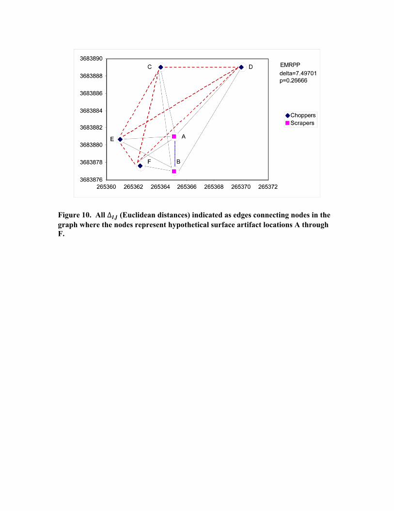
Figure 10. All ∆!,! (Euclidean distances) indicated as edges connecting nodes in the graph where the nodes represent hypothetical surface artifact locations A through F.

Table 3. Computation of delta for observed hypothetical distribution of scrapers and choppers in Figure 10. The observed Euclidean distances used in this computation are indicated as dashed edges in Figure 10.

AB; CDEF Number Artifact Pair Euclidean Distance (meters)

1 A, B Scraper-Scraper 4 2 C, D Chopper-Chopper 6 3 C, E Chopper-Chopper 8.825531145 4 C, F Chopper-Chopper 11.43283867 5 D, E Chopper-Chopper 12.24295716 6 D, F Chopper-Chopper 13.60403617 7 E, F Chopper-Chopper 3.367758899

Sum of Chopper-Chopper Euclidean distances 55.47312204 55.47312204/6 = 9.245520339 (2/6)*4+(4/6)*(9.245520339) delta = 7.49701355964778

Table 4. Delta values and corresponding P-values for each of the fifteen possible two- four combinations of hypothetical surface artifact locations A through F in Figure 10.

Order Combination Observed delta Probability (Exact) of a smaller or equal delta

1 CD; ABEF 4.625237699 1/15 = 0.0667 2 BF; ACDE 6.269733131 2/15 = 0.1333 3 EF; ABCD 6.960123351 3/15 = 0.2000

4* AB; CDEF 7.49701356 4/15 = 0.2667 5 BE; ACDF 7.673528201 5/15 = 0.3333 6 AF; BCDE 7.789464271 6/15 = 0.4000 7 AE; BCDF 7.858820482 7/15 = 0.4667 8 AD; BCEF 8.003970226 8/15 = 0.5333 9 CE; ABDF 8.145989313 9/15 = 0.6000

10 AC; BDEF 8.274176757 10/15 = 0.6667 11 BD; ACEF 8.764633501 11/15 = 0.7333 12 DE; ABCF 8.78498395 12/15 = 0.8000 13 CF; ABDE 9.159504623 13/15 = 0.8667 14 BC; ADEF 9.218536904 14/15 = 0.9333 15 DF; ABCE 9.244619921 15/15 = 1.0000

# of Permutations *Actual M=6! /(2! *4!)=15

Graph Theory and Network Analysis

Graph Theoretic Definitions Required in the Present Study

The first three of the following definitions are taken directly from Gross and Yellen (1999: 2,10, 48). Definition 1. A graph ! = !! ,!! is a mathematical structure consisting of two sets !!

and !! . The elements of !! are termed vertices (or nodes), and the elements of !! are

called edges. Each edge has a set of one or two vertices associated to it, which are known

as its endpoints. Definition 2. A graph is simple if it has neither self-loops nor multi-edges. Definition 3. A complete graph is a simple graph such that every pair of vertices is

joined by an edge.

Definition 4. A subgraph of a graph ! is a graph ! whose vertices and edges are all in

!.

Definition 5. A subgraph ! of !! ,!! is called a clique or maximal complete subgraph

of !! ,!! if every pair of vertices in ! is joined by at least one edge, and no proper

superset of ! has this property.

Definition 6. The adjacency matrix, !! , of a graph is a square matrix whose elements

!!" ! ≠ ! are 1 if nodes ! and ! are connected by an edge and 0 otherwise.

The Application of Graph Theory and Network Analysis in the Present Study

As was previously mentioned techniques from graph theory and network analysis

will be used to identify elements of tool kits in two contemporaneous maritime oriented

substantial habitation sites in southern California. The cultural chronology used presently

is that of King (1990: 28-44).

VEN-27 is a Middle to Late period or more specifically using King’s terminology

a Phase M5c- Phase L1c (A.D. 1050-1500) coastal Chumash village site, whereas SNI-25

is an exclusively Late period southern Channel Island village site whose time of

occupation (based on the previously mentioned calibrated radiocarbon dates) falls within

King’s Phase L1a- Phase L1c (A.D. 1225-1445). This means that VEN-27 and SNI-25

were occupied contemporaneously for a minimum of two hundred and twenty years.

Comparison of tool kits identified in the analysis of artifact types in VEN-27 and SNI-25

provide objective evidence in support of the proposition that there is a common regional

pattern in certain constituents of the material culture of Late period coastal hunter-

gatherer societies in southern California.

As mentioned previously, counts of typed artifacts from four excavated areas in

VEN-27 are used to construct a data matrix, which is used as raw data for a Pearson

correlation analysis. Next a cut off point for the correlation coefficient of the resulting

Pearson correlation matrix is determined. In this study it was determined that 0.78 is an

optimal cut off point for the correlation coefficient (c.c.). In this case all correlation

coefficients in the Pearson correlation matrix are coded 1 if they are in the interval

0.78 ≤ c.c. ≤ 1 and 0 if c.c. < 0.78. The coded correlation coefficients form an

adjacency matrix.

In the case of SNI-25 the Euclidean distances between all mapped surface

locations of a specific artifact type are used in the pair wise spatial analysis of selected

artifact types using exact multi-response permutation procedures (EMRPP) as described

in the previous section. The resulting P-values from these procedures are used to

construct an adjacency matrix. Here P-values ≤ 0.05 identify two artifact types whose

surface distribution within the sampling area of SNI-25 does not significantly overlap.

Therefore, in constructing this adjacency matrix P-values > 0.05 are coded 1 and P-

values ≤ 0.05 are coded 0. In both matrices 1 in the adjacency matrix represents a

connection between two artifact types and 0 an absence of a relationship. The resulting

adjacency matrix for both VEN-27 and SNI-25 is raw data, and are entered directly in the

form of an ASCII file (e.g. Microsoft Windows “Notepad”) into the UCINET 6 for

Windows software package (Borgatti, Everett, and Freeman 2002). In this study the

UCINET 6 software is used to identify what in graph theory, are known as cliques as well

as to draw network graphs. A mathematical procedure using methods from linear algebra

for detecting cliques is given in Harary and Ross (1957). The algorithm implemented in

UCINET 6 is given in Bron and Kerbosch (1973). The Bron and Kerbosch (1973)

algorithm finds all Luce and Perry (1949) cliques greater than a specified size. In the

context of the present study cliques are interpreted as tool kits and in the network graphs

labeled solid circles (nodes) depict artifact types and lines (edges) connecting nodes

depict a significant relationship between two artifact types. Here the relationship is

spatial co-occurrence.

Advantages of Graph-theoretic Methods over Data Reduction Methods and Clustering Procedures

The graph-theoretic methods used in this study are conservative in that no a priori

assumptions are made concerning the degree of homogeneity of the data being examined.

In fact, the internally cohesive groups (cliques) identified using graph theory result from

the structure of the data. Data reduction techniques such as principal components analysis

and factor analysis have been the preferred methods of archaeologists in the search for

‘tool kits’. A disadvantage in using such methods is that they are predicated upon

homogeneous data sets. This violates the very tenet of undertaking this kind of

exploratory analysis in the first place, which is the belief that the data are not

homogeneous (Read 1992). An advantage of using ordination techniques such as

principal components analysis on archaeological data is that they are effective at reducing

noise in data (Gauch 1982). Gauch (1982:1647) claims that eigenvector ordinations such

as those produced in principal components analysis are of three basic types:

(1) structure axes reflecting valid relationships, (2) spurious polynomial axes, and (3) noise axes.

The magnitude of the correlation coefficients of the type used in the VEN-27 analysis is

influenced by noise as well as the extent of linearity in the structure of the intrasite spatial

distribution of two artifact types. This means that the magnitude of a correlation

coefficient is not a definitive measure of proximity in a spatial relationship between a pair

of artifact types. The spatial association of artifact types is more realistically represented

by the binary structure of an adjacency matrix. The adjacency matrix is analogous to the

correlation matrix with much of the noise removed.

Another analytical approach often employed by archaeologists, in their search for

uncovering structure in heterogeneous data, has been to use one of the varied assortment

of clustering algorithms, (Read 1992).

Read and Russell (1996:4) comment on the improper use of these procedures in

archaeology.

Generally no precise criteria have been used in applications by archaeologists for deciding on the step that defines groups (Whallon 1990), and so groups determined are somewhat arbitrary.

A further disadvantage in using clustering procedures is that different algorithms produce

different results. Christenson and Read (1977) provide an archaeological example of this

dilemma.

CHAPTER 3 INTRASITE SPATIAL ANALYSIS

Definition of Activity Area A definition of an archaeological activity area is:

A spatially restricted area where a specific task or set of related tasks have been carried on, which is generally characterized by a scatter of tools, waste products, and/or raw materials; a feature, or set of features, may also be present (Flannery 1976:34).

Within the remnants of a specific type of activity area in an archaeological site it is

therefore expected that a characteristic sub-assemblage of the total assemblage of

artifacts contained within the site will repeatedly occur. Of the characteristic artifacts

comprising this sub-assemblage it is assumed that one or more (tool kits) used in specific

kinds of organized activities will be present. It is further assumed that the remaining set

of artifacts within an activity area will have a measurable non-random spatial

distribution. All of these assumptions rest on the tacit assumption that pre and post

depositional disturbances have not been sufficient to confound a meaningful intrasite

spatial analysis.

Dichotomy of House and Outdoor Activity Areas

In considering the distribution of utilitarian artifacts within a site, there are

apparent and consistent regional similarities in the way certain types of artifacts occur in

household activity areas and not in activity areas disjunctive from the locations of houses.

For example groundstone tools (e.g. manos and metates) primarily used in the processing

of plant materials appear to be universally linked to activity areas within or in close

proximity to houses. Groundstone tools are also strongly associated with women. As far

from Southern California as Mesoamerica, there is a strong connection between women

and the use of groundstone tools in household activity areas (Flannery and Winter 1976:

37). The linkage in the use of groundstone tools, women and household areas therefore

appears to be multi-regional and possibly universal. However, groundstone is but one

example of an apparent widespread pattern whereby certain utilitarian artifacts or sets of

such artifacts are associated with either male or female activities.

Criteria for Identifying House and Outdoor Activity Areas

House Locations and Activity Areas

A considerable amount of archaeological data pertaining to artifact types

associated with household activity areas in a maritime oriented southern California

prehistoric and historic substantial habitation site was gathered by members of the Van

Bergen-Los Angeles Museum Expedition of 1932. One of the goals of this expedition

was to collect more data on Chumash houses. In the pursuit of this goal the remains of

three houses (Houses A, B, and C) were completely excavated in the village of Muwu

(CA-VEN-11). The three houses were occupied into historic time by Chumash and were

in an excellent state of preservation at the time of their excavation. The village of Muwu

is located a few meters north east of Highway 1 (formerly Roosevelt Highway) on the

edge of a lagoon in the vicinity of Point Mugu in Ventura County (Woodward 1938:141).

Woodward (1932) gives the original description of the artifacts discovered in

Houses A, B, and C in the Muwu site. Based on these data I conjecture that the co-

occurrence and clustering of three of the artifact types found in House B in the 1932

excavation, as part of a non random surface artifact cluster, provides a non trivial

inference of a household location in a Middle to Historic period coastal village site in

Southern California. The presence of a surface cluster of fire affected rock (FAR) as part

of the total surface cluster strengthens this inference, and also indicates the location of a

hearth. The three artifact types are: (1) whole or fragmentary mortars, (2) whole or

fragmentary pestles, and (3) hammerstones. A detailed description of House B, which

includes mention of some of the cultural materials recovered from the floor of this

structure are given in (Gamble 1991:107). As will be discussed later, mortars, pestles,

and hammerstones are part of a household tool kit used in the processing and cooking of

food.

I propose that a second set of spatially co-occurring artifact types, as part of a

non-random surface artifact cluster, infer the location of a house. These artifact types are:

(1) hammerstones, (2) choppers, and (3) tarring pebbles. Archaeological evidence that

supports this proposal comes from House 3 in the Pitas Point site (VEN-27). Specifically,

a cluster consisting of four heavy hammerstones, four cobble choppers, and four tarring

pebbles was found in House 3 (Gamble 1983). As will be discussed later ethnography

suggests that choppers and hammerstones were used together in household areas in the

manufacture of groundstone tools, such as mortars and pestles. Ethnography also

suggests that tarring pebbles were used exclusively for sealing a specialized type of

watertight basket known as a “water bottle”. Additional ethnographic evidence strongly

links most types of basket making to household areas.

Outdoor Activity Area Locations

I propose that the co-occurrence of hammerstones (especially flaking hammers),

scrapers (carinate, domed, flake, etc.), and flakes as part of a non random surface artifact

cluster that has a low relative frequency of whole or fragmentary mortars, is an objective

and sufficient criterion for identifying the location of an area of outdoor activities in a

Middle to Historic period coastal village site in southern California. It is expected that

discrete and more homogeneous surface artifact clusters are present within such a cluster,

and identify specific activity areas. For example, Area 1 in the Pitas Point site (VEN-27)

has been interpreted as an outdoor activity area adjacent to a house (Gamble 1983).

Within this area flake clusters that co-occur with concentrations of bone are seen as

probable butchering areas (Gamble 1983). In addition, a large number of flake and

domed scrapers, as compared to Areas 2, 3, and 5 in VEN-27, were recovered in Area 1.

The high frequency of domed scrapers in Area 1 may indicate the manufacture of wood

plank canoes (Gamble 1983).

Locations of House and Outdoor Activity Areas in the Sample Area of SNI-25

Methods of Analysis

Nearest Neighbor Analysis

The statistically significant results using the previously described nearest

neighbor analysis for the mapped surface artifacts in the SNI-25 sampling area are given

in Table 5 and visually depicted in Figure 11. As is apparent from Table 5 the significant

values of the Clark and Evans nearest neighbor statistic for the sampling area in SNI-25

are all less than one, which indicates clustering in these groups of surface artifacts. This

agrees with

the intuitive expectation that surface artifacts should have a close spatial association in

activity areas within an archaeological site. Also, as can be seen in Table 5, the Clark and

Evans nearest neighbor statistic is smaller in every case for mapped surface artifacts

within what are interpreted as house activity areas than for what are interpreted as

outdoor activity areas in the sampling area in SNI-25. This means that within the SNI-25

sampling area the surface artifacts within what are interpreted, as house activity areas are

more tightly clustered than the surface artifacts within what are interpreted as outdoor

activity areas. This result makes sense when one considers that many of the outdoor

activities that probably occurred at SNI-25 including the repair and maintenance of open

ocean watercraft such as wood plank canoes or the construction of near shore fishing

platforms such as driftwood rafts required more room than typical household activities

such as cooking.

Table 5. Results of the nearest neighbor analysis of the surface artifact sample at CA-SNI-25.

Interpretation of Results

SNI-25 Activity Areas

Figures 12, 13, 14, and 15 provide a visual depiction of statistically significant

clusters of mapped and typed surface artifacts in what are interpreted as house activity

areas within the sampling area of SNI-25. Refer to Appendix E for representative SNI-25

artifacts. Two identifiable types of activity loci within what may be the areal extent of

individual houses are apparent in these figures. As will be discussed in detail later, the

results of the network analyses of artifact types from VEN-27 and SNI-25 support the

proposition that mortars and pestles are tools used in the preparation of food in house

Easting (interval)

Northing (interval)

Clark & Evans

Nearest Neighbor Statistic

P-value

No. of Surface Artifact

Locations

No. of iterations

used to compute the approximate

sampling distribution

Interpreted Type of Activity

Area

355-360 910-915 0.48 0.003 7 1000 House 355-360 915-920 0.11 0 10 1000 House 360-365 915-920 0.52 0.002 12 1000 House 365-375 900-910 0.52 0.002 12 1000 House 365-370 910-915 0.33 0.0001 6 1000 House 370-375 910-915 0.46 0.002 4 1000 House 360-365 875-880 0.29 0.001 3 1000 House 360-365 880-885 0.33 0.007 6 1000 House

365-370 880-885 0.84 0.055

14 1500 Outdoor

365-367.5 877.5-880 0.78 0.067

7 1500 Outdoor

360-375 885-900 0.56 0.001 14 1000 Outdoor

Figure 11. SNI-25 sampling area with plotted positions of surface artifacts designated as belonging to one of the six interpreted activity areas.

activity areas and not outdoor activity areas. Ethnohistoric and ethnographic data as will

be given later also supports this conclusion. The first identifiable type of activity locus

consists of a cluster of surface artifacts that includes mortar fragments. This suggests that

food processing occurred in this type of activity locus. Also, in the case of House

Activity Area #1 the association of fire-affected rock (FAR) with the mortar fragments in

one locus suggests the presence of a hearth, which in combination with the mortar

fragments implies both the preparation and cooking of food (Figure 12).

Figure 12. House Activity Area #1.

The second type of identifiable activity locus that is present in what are

interpreted as house activity areas in SNI-25 consists of a cluster of surface artifacts that

are mostly metavolcanic and/or quartzite flakes. Note that in my analysis the separate

morphology-based artifact types of debitage and flake in the official San Nicolas Island

lithics typology are merged into a single “functional” type of artifact, which I call

“flake”. This is because the sharpness and shape of the edges of a “flake” relate directly

to its use as a scraping, sawing, cutting, boring or perforating implement and not the

presence or absence of a percussion bulb, which is the main criterion used to differentiate

flakes and debitage in the San Nicolas Island lithics typology. It is probable that some of

the longer quartzite and metavolcanic flakes in my sample are unifacially retouched and

therefore could be typed as flake scrapers. In a later section the information obtained

from the results of replicative experimentation and microwear analysis are used to

connect flake length with use in SNI-25. Based on these results it is inferred that meat

cutting/butchery and/or wood, small bone, and shell working were the principle activities

that took place in the second identifiable type of activity locus within house activity areas

in SNI-25.

Also, House Activity Area #4 (Figure 13) is more than fifteen meters south of the

other three interpreted house activity areas within the sampling area. Based on my

observations of surface artifacts outside my sampling universe, it is suggested that House

Activity Area #4 is part of a separate and more interior cluster of houses. Also, House

Activity Area #4 is situated immediately to the west of what has been interpreted as

Outdoor Activity Area #2.

Figure 13. House Activity Area #4 and two adjacent small outdoor activity areas.

Outdoor Activity Area #2 (Figure 14) has a much denser as well as noticeably different

and more heterogeneous composition of surface artifacts as compared to the other

interpreted outdoor activity area in the sampling area, Outdoor Activity Area #1 (Figure

15). For example, several of the surface artifacts in Outdoor Activity Area #2 include one

of a kind types in the sample, such as half of a donut-shaped steatite artifact with

asphaltum repair (Figure 18), a small chunk of sandstone with pitting on one surface, and

a sandstone pestle fragment that appears to have been used as an abrader (Figure 19).

Figure 14. Outdoor Activity Area #2 and two small outdoor activity areas.

Also, clusters of broken donut-shaped stones larger than the preceding SNI-25 artifact

have been observed only in interior sites of San Clemente Island, in areas where

Dichelostemma capitatum (blue dicks) are common (J. Cassidy 2004, personal

communication).

Figure 15. Outdoor Activity Area #1.

Because of the small size of the SNI-25 donut stone fragment it is not likely this artifact

in its complete form was used as a digging stick weight. It is possible that this artifact

was part of a sun stick or some other ritual object (C. King 2004, personal

communication). These observed differences in artifact composition of House Activity

Area #4 suggest this area may not be contemporaneous with House Activity Areas #1, 2

(Figure 16), and 3 (Figure 17). In the event House Activity Area #4 is contemporaneous

with the other three house activity areas maybe House Activity Area #4 is the remnant of

the household of an SNI-25 inhabitant of high social rank such as a chief.

Figure 16. House Activity Area #2.

Figure 17. House Activity Area #3 and adjacent small outdoor activity area.

The relatively higher density and diversity of the surface artifact types in Outdoor

Activity Area #2 compared to the other surface artifact clusters in the sampling area

points to this possibility. Considering social organization at SNI-25, if House Activity

Area #4 is contemporaneous with House Activity Areas #1,2, and 3 and is part of a

second and well-demarcated house cluster from that of the first three house activity areas,

this suggests the possibility that each house cluster belongs to a separate kinship group.

Dual organization or more specifically a moiety system such as existed in a number of

southern California Uto-Aztecan speaking groups (e.g. Serrano) is inferred in this case. In

the case that House Activity Area #4 is not contemporaneous with House Activity Areas

#1,2, and 3, it remains unequivocal that House Activity Areas #1,2, and 3 form a tight

cluster at the northern edge of the site. The close proximity of these three house activity

areas to one another suggests not only that they co-occur in time but also are part of a

single kinship group, possibly an extended family.

Figures 11 and 12 provide an illustration of what have been interpreted as outdoor

activity areas in the sampling area of SNI-25. Outdoor Activity Area #1 is interior to all

other interpreted activity areas in the sampling area of SNI-25. Because Outdoor Activity

Area #1 is enclosed by a rather large sampling quadrat (15 x 15 meters) compared to the

other sampling quadrats, it is less certain if all of the inferred activity loci within this

activity area overlap in time. Some of the surface artifacts in Outdoor Activity #1 are

much closer to House Activity Areas #1, 2, and 3 than they are to either House Activity

Area #4 or Outdoor Activity Area #2. The converse is also true. Specifically, clusters of

surface flakes are more numerous and on average are larger in total number in two

aggregates of surface artifacts close to House Activity Area #4 and Outdoor Activity

Area #2. It is also possible that House Activity Area #4, if contemporaneous with House

Activity Areas #1, 2, and 3, was the residence of craft specialists who made and repaired

fine utilitarian objects that included both sandstone mortars and pestles. This possibility

is manifested by the presence of the apparent sandstone abrader, whose utilized edge is

concave and of the right curvature to suggest use in the final shaping and smoothing of

mortar rims and/or pestles. Also, a chopper/hammer is a close neighbor to the sandstone

abrader, and as will be discussed later, choppers and hammer stones appear to have been

the primary pecking tools used in the manufacture of groundstone utilitarian objects at

the multi-regional level.

Tool Kits and Activity Areas in the Pitas Point Site (VEN-27)

In this section the counts of twenty-one artifact types from four of five areas

excavated by Chester King and others in the Pitas Point site, VEN-27 are re-examined in

the attempt to elucidate specific tool associations or tool kits. These areas are given as

Areas 1, 2, 3, and 5 in Gamble (1983). Complete provenience data of the excavated

VEN-27 artifacts exists (C. King 2004, personal communication) but was not available to

me at the time I did the analysis of the artifact data from this site. Therefore as analyzed

in this thesis the VEN-27 artifact data are taken from a three-dimensional archaeological

space but lack point provenience at the individual artifact level, as is the case with the

SNI-25 data.

These data from VEN-27 along with providing a much larger sample than the surface

sample taken at SNI-25 contain types of artifacts all of which are present at SNI-25. Also,

the period of occupation of VEN-27 has a considerable overlap with SNI-25, and both

sites were heavily dependent on a very similar assemblage of marine resources. It is

therefore reasonable to assume that the organizational structure of the artifact assemblage

at VEN-27 might be quite similar to that of SNI-25. Tool kits not present in the SNI-25

sample but present in the site might therefore be predicted in the analysis of the VEN-27

artifact counts. Analysis of the VEN-27 artifact data also provides for a comparison of

two roughly contemporaneous maritime-based hunter-gatherer substantial habitation sites

widely separated by open ocean. It is known that the people who occupied VEN-27 were

Chumash but the actual cultural affiliation of the people of San Nicolas Island is not

known.

Martz (2002:3) makes the following statement in support of the expected

similarities in many of the activities that took place in the lives of the San Nicolas

Islanders and coastal Chumash and Gabrieleno.

The lifestyle (of the people of San Nicolas Island) appears to have been quite similar to that of the marine oriented Chumash and Gabrieleno who occupied the Channel Islands and adjacent coastline of Southern California at the time of European contact. As has already been mentioned Pitas Point is a substantial Chumash habitation

site. The site is located approximately eight miles northwest of Ventura, California and is

adjacent to both Highway 101 and the ocean. The site area encompasses both sandy

beach and the top of a low-lying colluvial terrace immediately behind the beachfront.

Area 1 is located on the beach and contains dark, organically enriched sand. (Gamble

1983) interpreted this location as an area of outdoor activity. Areas 2, 3, and 5 are located

on the terrace. Area 2 is farthest from the beach. (Gamble 1983) interpreted Areas 3 and 5

as containing portions of houses. During the time the site was occupied Area 1 was

directly below Area 3. Gamble (1983) gives the counts of 21 artifact types from each of

the five excavated areas in Table 1 of her paper. She then analyzes these data to test the

hypothesis (using chi-square tests) that within the site there are statistically significant

differences in the types of artifacts occurring within houses as compared to those

occurring in areas of outdoor activity. The conclusion of her analysis is to accept the

hypothesis.

Methods of Analysis

Correlation Analysis

The frequency data in Table 6 were used to compute a Pearson correlation matrix,

Table 7. This method of analysis has already been discussed in a previous section.

To connect the correlation coefficient with tool kits it is necessary to make the

following assumption: Assume that pairs of artifact types that consistently move together

in terms of abundance between locations in a site are functionally associated. In other

words when two artifact types belong to at least one identical and consistent grouping or

aggregate of artifact types (tool kit) they can be directly linked to a specific range of

organized human activities that repeatedly occurred within a site over time. In the next

step in the analysis the correlation matrix will be transformed into an adjacency matrix.

As was mentioned earlier the adjacency matrix will form the basis for discovering tool

kits using the UCINET 6 network analysis software (Borgatti, Everett, and Freeman

2002) to identify cliques.

Network Analysis

For this analysis a cut-off point of 0.78 for the correlation coefficient was selected

as a result of the following procedure. The resulting adjacency matrix is given as Table 8.

As was mentioned earlier the adjacency matrix is the raw data used in a network analysis.

The two network graphs in this thesis were drawn using the net-draw program, which is

part of the UCINET 6 software. Text was added to each of the network graphs using

UCINET 6 Netdraw, Corel 7 Draw (SNI-25 graph), and Microsoft Word (VEN-27

graph). Ellipses were added to the network graphs using Corel 7 Draw (SNI-25 graph)

and Microsoft Excel (VEN-27 graph).

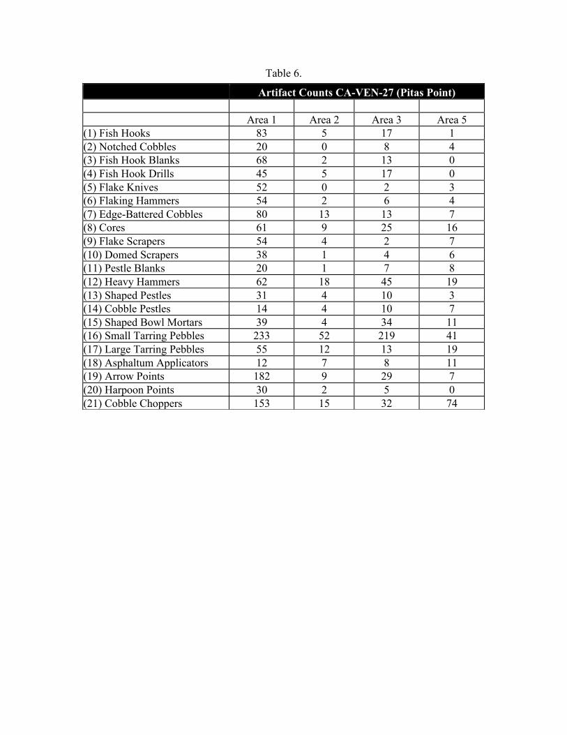
Table 6.

Artifact Counts CA-VEN-27 (Pitas Point) Area 1 Area 2 Area 3 Area 5

(1) Fish Hooks 83 5 17 1 (2) Notched Cobbles 20 0 8 4 (3) Fish Hook Blanks 68 2 13 0 (4) Fish Hook Drills 45 5 17 0 (5) Flake Knives 52 0 2 3 (6) Flaking Hammers 54 2 6 4 (7) Edge-Battered Cobbles 80 13 13 7 (8) Cores 61 9 25 16 (9) Flake Scrapers 54 4 2 7 (10) Domed Scrapers 38 1 4 6 (11) Pestle Blanks 20 1 7 8 (12) Heavy Hammers 62 18 45 19 (13) Shaped Pestles 31 4 10 3 (14) Cobble Pestles 14 4 10 7 (15) Shaped Bowl Mortars 39 4 34 11 (16) Small Tarring Pebbles 233 52 219 41 (17) Large Tarring Pebbles 55 12 13 19 (18) Asphaltum Applicators 12 7 8 11 (19) Arrow Points 182 9 29 7 (20) Harpoon Points 30 2 5 0 (21) Cobble Choppers 153 15 32 74

Table 7. Pearson correlation coefficient matrix computed from the data in Table 6.

Procedure for Determining the Optimal Cut-off for the Correlation Coefficient

(1) Plot the frequencies of the correlation coefficients in the Pearson correlation

matrix. (2) Starting at 1 in this plot, move in the negative direction along the x-axis until

the first zero frequency, or until the first significant “gap” of constant frequency is

encountered. In the case of the VEN-27 correlation coefficient frequency plot (Figure 20)

this occurs at (0.79, 0.8,0.81). (3) The correlation coefficient at one of the ends of the

“gap” is predictably optimal, in that it should produce a locally parsimonious result with

respect to the cliques identified in the network analysis. To illustrate what I mean observe

the results of the network analyses using the correlation coefficients immediately above

and below the suggested optimal value of 0.78 for the VEN-27 matrix as cut-offs. Note

that the number of cliques increases from four to six, going from 0.78 to 0.79, and from

four to five, going from 0.78 to 0.77. In fact the number of cliques continues to increase

in both directions away from 0.78. For example, using 0.8 as a cut-off results in eight

cliques.

1 0.96 1 0.98 0.98 0.99 0.99 0.98 0.97 0.97 0.92 0.9 1 0.88 0.77 0.75 0.96 0.63 1 1 0.87 0.96 1 0.96 0.96 0.94 0.95 0.92 0.99 0.91 0.95 0.97 0.95 0.97 0.98 0.88 0.82 0.92 0.71 0.96 0.95 0.89

1 0.96 1 0.98 0.98 0.99 0.99 0.99 0.97 0.98 0.92 0.9 1 0.89 0.78 0.75 0.96 0.64 1 1 0.87 0.98 0.96 0.98 1 0.93 0.95 0.95 0.97 0.9 0.92 0.88 0.95 0.99 0.91 0.85 0.85 0.89 0.52 0.97 0.98 0.78 0.98 0.94 0.98 0.93 1 1 0.99 0.97 1 1 0.94 0.82 0.97 0.84 0.68 0.63 0.99 0.73 0.99 0.99 0.93 0.99 0.95 0.99 0.95 1 1 0.99 0.98 0.99 1 0.94 0.84 0.98 0.85 0.71 0.66 0.99 0.71 1 0.99 0.92 0.99 0.92 0.99 0.95 0.99 0.99 1 0.96 0.99 0.98 0.9 0.83 0.98 0.82 0.68 0.65 0.97 0.64 1 1 0.88 0.98 0.99 0.99 0.97 0.97 0.98 0.96 1 0.94 0.97 0.97 0.93 0.99 0.95 0.84 0.79 0.95 0.71 0.98 0.98 0.9 0.97 0.91 0.97 0.9 1 0.99 0.99 0.94 1 0.99 0.93 0.77 0.95 0.8 0.62 0.56 1 0.74 0.98 0.97 0.94 0.97 0.95 0.98 0.92 1 1 0.98 0.97 0.99 1 0.96 0.82 0.96 0.85 0.69 0.62 1 0.77 0.99 0.98 0.95 0.92 0.97 0.92 0.88 0.94 0.94 0.9 0.97 0.93 0.96 1 0.84 0.92 0.93 0.78 0.67 0.95 0.86 0.93 0.91 0.97 0.9 0.95 0.9 0.95 0.82 0.84 0.83 0.93 0.77 0.82 0.84 1 0.92 0.96 0.97 0.96 0.77 0.47 0.87 0.88 0.69 1 0.97 1 0.99 0.97 0.98 0.98 0.99 0.95 0.96 0.92 0.92 1 0.9 0.81 0.79 0.94 0.61 0.99 0.99 0.85

0.88 0.98 0.89 0.91 0.84 0.85 0.82 0.95 0.8 0.85 0.93 0.96 0.9 1 0.95 0.88 0.82 0.67 0.87 0.86 0.81 0.77 0.88 0.78 0.85 0.68 0.71 0.68 0.84 0.62 0.69 0.78 0.97 0.81 0.95 1 0.98 0.64 0.43 0.74 0.74 0.6 0.75 0.82 0.75 0.85 0.63 0.66 0.65 0.79 0.56 0.62 0.67 0.96 0.79 0.88 0.98 1 0.56 0.25 0.71 0.72 0.48 0.96 0.92 0.96 0.89 0.99 0.99 0.97 0.95 1 1 0.95 0.77 0.94 0.82 0.64 0.56 1 0.8 0.97 0.96 0.97 0.63 0.71 0.64 0.52 0.73 0.71 0.64 0.71 0.74 0.77 0.86 0.47 0.61 0.67 0.43 0.25 0.8 1 0.67 0.63 0.93

1 0.96 1 0.97 0.99 1 1 0.98 0.98 0.99 0.93 0.87 0.99 0.87 0.74 0.71 0.97 0.67 1 1 0.89 1 0.95 1 0.98 0.99 0.99 1 0.98 0.97 0.98 0.91 0.88 0.99 0.86 0.74 0.72 0.96 0.63 1 1 0.87

0.87 0.89 0.87 0.78 0.93 0.92 0.88 0.9 0.94 0.95 0.97 0.69 0.85 0.81 0.6 0.48 0.97 0.93 0.89 0.87 1

Table 8. Adjacency matrix resulting from the binary coding of the correlation coefficient matrix in Table 7 using a cut-off for the correlation coefficient of 0.78.

1 2 3 4 5 6 7 8 9 10 11 12 13 14 15 16 17 18 19 20 21

-- -- -- -- -- -- -- -- -- -- -- -- -- -- -- -- -- -- -- -- --

1 0 1 1 1 1 1 1 1 1 1 1 1 1 1 0 0 1 0 1 1 1

2 1 0 1 1 1 1 1 1 1 1 1 1 1 1 1 1 1 0 1 1 1

3 1 1 0 1 1 1 1 1 1 1 1 1 1 1 0 0 1 0 1 1 1

4 1 1 1 0 1 1 1 1 1 1 1 1 1 1 1 1 1 0 1 1 1

5 1 1 1 1 0 1 1 1 1 1 1 1 1 1 0 0 1 0 1 1 1

6 1 1 1 1 1 0 1 1 1 1 1 1 1 1 0 0 1 0 1 1 1

7 1 1 1 1 1 1 0 1 1 1 1 1 1 1 0 0 1 0 1 1 1

8 1 1 1 1 1 1 1 0 1 1 1 1 1 1 1 1 1 0 1 1 1

9 1 1 1 1 1 1 1 1 0 1 1 0 1 1 0 0 1 0 1 1 1

10 1 1 1 1 1 1 1 1 1 0 1 1 1 1 0 0 1 0 1 1 1

11 1 1 1 1 1 1 1 1 1 1 0 1 1 1 0 0 1 1 1 1 1

12 1 1 1 1 1 1 1 1 0 1 1 0 1 1 1 1 0 0 1 1 0

13 1 1 1 1 1 1 1 1 1 1 1 1 0 1 1 1 1 0 1 1 1

14 1 1 1 1 1 1 1 1 1 1 1 1 1 0 1 1 1 0 1 1 1

15 0 1 0 1 0 0 0 1 0 0 0 1 1 1 0 1 0 0 0 0 0

16 0 1 0 1 0 0 0 1 0 0 0 1 1 1 1 0 0 0 0 0 0

17 1 1 1 1 1 1 1 1 1 1 1 0 1 1 0 0 0 1 1 1 1

18 0 0 0 0 0 0 0 0 0 0 1 0 0 0 0 0 1 0 0 0 1

19 1 1 1 1 1 1 1 1 1 1 1 1 1 1 0 0 1 0 0 1 1

20 1 1 1 1 1 1 1 1 1 1 1 1 1 1 0 0 1 0 1 0 1

21 1 1 1 1 1 1 1 1 1 1 1 0 1 1 0 0 1 1 1 1 0

Figure 20. Plot of the frequencies of the correlation coefficients from Table 7.

It is clear that moving in either direction away from 0.78 for the VEN-27 data results

not only in more cliques, but also in greater redundancy in their composition. It is posited

here that redundancy in the cliques reflects redundancy and therefore structure in the

data. Gauch (1982:1647) comments on the relationship between redundancy and structure

in data “… data structure is discriminated from noise by having redundant patterns in

species abundances”. Minimizing data redundancy is one of the uses of multivariate

techniques such as principal components analysis. Reduction in dimensionality of

multivariate data sets is often required to reveal latent structure hidden by redundancy. I

suggest that in the case of cliques, a clique with greater parsimony better represents the

latent structure of the data (Tables 9, 10, and 11).

Table 9. Using 0.77 as a cut-off.

Table 10. Using 0.78 as a cut-off.

Table 11. Using 0.79 as a cut-off.

The Network Graph of Artifact Types in CA-VEN-27

The artifacts comprising each of the four cliques or maximal complete subgraphs in

the network graph are listed in Table 12. The four cliques in the network graph of VEN-

27 (Figure 21) are outlined with ellipses. The artifact types within a clique are connected

by a line to each of the other artifact types of artifacts in the clique. Cliques 1, 3, and 4

are interpreted as household tool kits and Clique 2 is interpreted as an outdoor activity

area tool kit. Artifact types that appear to be linked to specialized activities occur on a

4 cliques found. 1: 1 2 3 4 5 6 7 8 9 10 11 13 14 17 19 20 21 2: 1 2 3 4 5 6 7 8 10 11 12 13 14 19 20 3: 2 4 8 12 13 14 15 16 4: 11 17 18 21

5 cliques found. 1: 1 2 3 4 5 6 7 8 9 10 11 12 13 14 17 19 20 2: 1 2 3 4 5 6 7 8 9 10 11 13 14 17 19 20 21 3: 1 2 3 4 8 11 12 13 14 15 4: 2 4 8 12 13 14 15 16 5: 10 11 17 18 21

6 cliques found. 1: 1 2 3 4 5 6 7 8 9 10 11 13 14 17 19 20 2: 1 2 3 4 5 6 7 8 10 11 12 13 14 19 20 3: 2 4 8 12 13 14 15 4: 2 4 12 14 15 16 5: 1 2 3 5 6 7 8 9 10 11 13 14 17 19 20 21 6: 11 17 18 21

single clique. These artifacts are identified in Table 12 with a star (*). Flake scrapers

occur only in Clique 1 and may have been used in household activities such as

woodworking (e.g. manufacture of wooden bowls). Bowl mortars and small tarring

pebbles occur only in Clique 3. Both ethnohistory and ethnography confirm that bowl

mortars in combination with pestles were used in household areas to pulp large seeds

such as cherry pits (Prunus illicifolia) and acorns (Quercus sp.) and, in maritime

environments such as Pitas Point and San Nicolas Island, to tenderize abalone meat

(Haliotis sp.). Ethnohistory assigns tarring pebbles to the very specific task of coating the

interior of water storage baskets with asphaltum. As will be discussed in detail in a later

section, tarring pebbles size classes exist, and small tarring pebbles are logically

associated with the sealing of portable water storage baskets, often referred to as

canteens.

Table 12. Resulting cliques that are interpreted as either house or outdoor activity area tool kits.

A network graph is an elegant depiction of a complex system of interrelationship

and interaction. Figure 21 provides a direct visualization of the intricate system that

constitutes the intrasite spatial relationships of a large number of artifact types. A graph

such as Figure 21 is more than just a picture, it is a statistical model whose structure is

amenable to a broad range of mathematical analysis using concepts embodied in graph

theory, For example the degree of the nodes (number of incident edges) of Figure 21

provides an objective measure of the interrelationship of one artifact type with other

artifact types in the assemblage. In the case of asphaltum applicators, the node depicting

this artifact type has the lowest degree in the network graph. This node shares edges only

Clique 1 Clique 2 Clique 3 Clique 4

Fish Hooks Fish Hooks Notched Cobbles Pestle Blanks

Notched Cobbles Notched Cobbles Fish Hook Drills Large Tarring

Pebbles

Fish Hook Blanks Fish Hook Blanks Cores Asphaltum

Applicators* Fish Hook Drills Fish Hook Drills Heavy Hammers Cobble Choppers

Flake Knives Flake Knives Shaped Pestles Flaking Hammers Flaking Hammers Cobble Pestles

Edge-Battered Cobbles

Edge-Battered Cobbles

Shaped Bowl Mortars*

Cores Cores Small Tarring

Pebbles* Flake Scrapers* Domed Scrapers Domed Scrapers Pestle Blanks

Pestle Blanks Heavy Hammers Shaped Pestles Shaped Pestles Cobble Pestles Cobble Pestles

Large Tarring Pebbles Arrow Points Arrow Points Harpoon Points

Harpoon Points Cobble Choppers

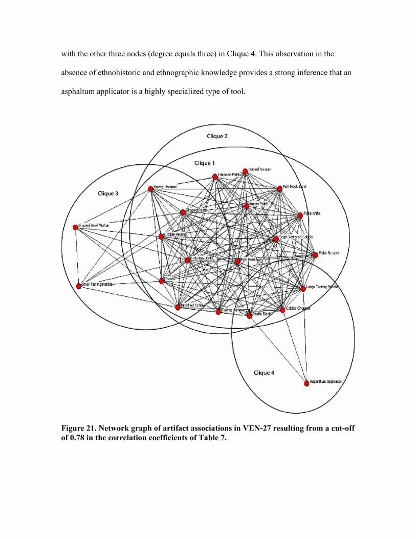
with the other three nodes (degree equals three) in Clique 4. This observation in the

absence of ethnohistoric and ethnographic knowledge provides a strong inference that an

asphaltum applicator is a highly specialized type of tool.

Figure 21. Network graph of artifact associations in VEN-27 resulting from a cut-off of 0.78 in the correlation coefficients of Table 7.

Interpretation of Results

It is very likely there is an intrasite spatial dimension to tool kits in the Pitas Point

site. A conclusion concerning the spatial distribution of some of the artifact types at Pitas

Point is a follows:

One of the conclusions derived from the foregoing observations, maps, figures, and significant chi-square values is that certain artifact types occurred more frequently in certain areas of the site than others (Gamble 1983:120).

Outdoor Activity Area Tool Kits in VEN-27

Clique 2 is interpreted as an outdoor activity area tool kit. It should be noted that in

southern California some outdoor activity aras are believed to be strongly but not

exclusively associated with men (C, King 2003, personal communication). Therefore

Clique 2 as interpreted has a strong male gender component. Both Cliques 1 and 2 place

notched cobbles, fishhook blanks, fishhook drills, shaped cobbles, and cobble pestles in

association. As can be seen in Figure 21 they are in relatively close association compared

to the other artifacts in these cliques. As will be discussed in the next section Clique 1 is

interpreted as a house area tool kit. Apparently the manufacture and maintenance of

fishing equipment occurred in both house and outdoor activity areas at the Pitas Point

site. The close association of notched cobbled with both pestles and fishing equipment

suggests the possibility of functionally distinct tool types in the existing category of

notched cobbles. It is plausible that notched cobbles were a multipurpose tool type. It is

certain that some of the stone objects typed as notched cobbles at Pitas Point were used as

net weights. However, the connection of notched cobbles to shaped and cobble pestles in

Cliques 1 and 2 suggests that some of the Pitas Point stone tools presently typed as

notched cobbles may have been used in the processing of plant materials. The fishhooks

at Pitas Point are all made out of California mussel (Mytilus californianus). A small

hammerstone, probably an end battered cobble hammer or some similar type was used in

the initial step of manufacture of these fishhooks. The use of hammerstones in fishhook

manufacture is supported both ethnographically and ethno historically.

Hamy (1963) and others have written descriptions of the manufacture of the shell fishhook. Hoover has summarized the data as follows: A roughly circular piece of shell was broken off with a hammerstone and was crudely retouched to form an approximate triangle. The center of the disc was perforated with a chert drill, using an abrasive paste of water and sand (Hudson and Blackburn 1979:173).

Arrow and harpoon points are also found in both Cliques 1 and 2 and are closely

associated with each other and flake knives as can be seen in Figure 21. Note that flake

knives in the Pitas Point typology correspond to utilized flakes and utilized debitage in

the lithic typology currently in use for San Nicolas Island. Gamble (1983:122) sees the

majority of the Pitas Point flake knives as butchering implements, noting:

The flake knives examined at Pitas Point all had edge angles under 60 degrees and utilization scars on both faces of the utilized edge, indicating a cutting or sawing motion (Tringham et. al. 1974). In butchering experiments with sea mammals, it was found that flake knives with no retouch were more effective in butchering tasks than bifacially flaked tools (Walker 1978).

Obviously arrow and harpoon points are hunting implements and it is plausible that flake

knives were used for cutting purposes in the manufacture and maintenance of the

components of arrow and harpoon shafts and poles, as well as for the slicing of meat. The

use of wooden harpoon poles by a group on Catalina Island in 1602 is confirmed by Fr.

Antonio de la Ascension.

In the island there are many elder trees [Sambucus mexicana], which grow some long slender poles. The Indians use these for fishing, as our people do harpoons. At the end of the pole they fasten a harpoon made of fishbone, and to this they tie firmly a long strong line like twine [Wagner 1929: 236].

I think it is more than an intriguing possibility that the SNI-25 inhabitants may have

traded with the Catalina Islanders for carefully selected elderberry branches, which were

carved on site into harpoon poles, using flake knives. Unfortunately wooden cultural

objects are rarely preserved in archaeological sites and it is unlikely that a whole or even

fragmentary wooden harpoon pole will be discovered in the present and future

excavations at SNI-25.

By definition flaking hammers are used in the manufacture of flake tools, such as

flake knives. It is plausible that edge-battered cobbles were used at Pitas Point to produce

large flakes, some of which found immediate use as flake knives. Notched cobbles and

heavy hammers occur in both Cliques 2 and 3. Ethnographic data suggest that one of the

uses of heavy hammers was in the manufacture of notched cobbles, which were then used

as fishing net weights. Hudson and Blackburn (1979:160) state, “the Indians apparently

selected a simple beach cobble for modification and pecked a groove or notched the

stone”.

In the following section Clique 3 is interpreted as a household tool kit. This

provides objective evidence that notched cobbles were made in outdoor activity areas and

at least stored in houses. The following supports the view of notched cobbles as fishing

net weights.

…there is ample evidence of stone net weights along the entire coastal area of the Chumash (Pilling 1951; Rogers 1929: 404-405). Some of these

specimens have circumferential grooves or have side or end notches for the attachment of the net (Hoover 1973:7).

Clique 2 also contains domed scrapers. At Pitas Point these tools are relatively small and

made of chert. Domed scrapers could have been used in outdoor activity areas for

woodworking, and specifically in the construction and maintenance of the tomol, or plank

canoe.

Boat construction and maintenance probably occurred in the beach zone. A high percentage of domed scrapers was found in Areas 1 and 5. Perhaps these were employed to shape planks used in canoe building (Gamble 1983:121).

House Activity Area Tool Kits in VEN-27

Clique 1 is interpreted as a tool kit used in household activity areas because it

contains large tarring pebbles. Clique 4, which will be discussed later also contains large

tarring pebbles. From ethnography we know the Chumash used tarring pebbles to seal the

interior of a specialized type of basket called a “water bottle”. Bryan (1970:130) cites the

recovery of a badly disintegrated “water bottle” on San Nicolas Island “150 yards south

and west of the Coney Point survey monument”. Hudson and Blackburn (1986:174)

describe the form and use of the tarring pebble as:

A small rounded, unmodified stone which is heated and used to apply a thin layer for waterproofing purposes to the inside of certain baskets.

Clearly water bottle production and use is therefore expected in SNI-25 since an

abundance of tarring pebbles have been found in an ongoing excavation at this site. Large

tarring pebbles were likely used in the manufacture of large water bottles. Hudson and

Blackburn (1983:51) describe the large water bottle as:

A twined, asphaltum-covered basket with a somewhat tubular shape, used for storing large quantities of water.

Ethnography establishes the manufacture of basketry as an activity occurring in

household areas and the large water bottle as a household item. Hudson and Blackburn

(1983:51) comment on the use of large water bottles in houses. The suggestion that large

water bottles were especially made for household use first appeared in vocabulary data

collected by Henshaw, in that his consultants supplied a specific term for “a large water

jug for holding water in the house” (Heizer 1955:102).

Clique 1 also contains cobble choppers, and domed scrapers. Cobble choppers

undoubtedly could be used for a multiplicity of tasks, which probably include the

chopping of bone and wood. Keeley (1980:146) cites a “pointed chopper-core with a

cortex-covered butt” (lithic HXN 637) as probably having been used for chopping bone.

This interpretation is based on the microwear polish of this tool, which Keeley says is

“bright but rough and sometimes pitted”. The morphology of this chopper-core is very

similar to many of the choppers in the excavated VEN-27 sample and especially the

choppers in the SNI-25 surface sample.

Choppers and large tarring pebbles may well have been used together in the

manufacture of large water bottles. Choppers may have been used to cut the plant fibers

woven into water bottles and to pulverize the asphaltum used to make them water tight.

Large water bottles were likely important at sites like Pitas Point and many of the sites on

the Channel Islands such as SNI-25 where good sources of freshwater were somewhat

distant. An account from Fr. Antonio de la Ascension at the middle of Catalina Island

before his group got to the Isthmus supports this assertion.

Our people asked them by signs for water. They at once brought a rush barrel full of water, which was good, and said that the spring from which they took it was somewhat distant. (Wagner 1929: 236)

Water storage would have likely been of considerable importance in substantial

habitation sites such as Pitas Point and SNI-25 that were not in juxtaposition to a

perennial stream or other permanent water source. The impetus for the development of

craft specialization in VEN-27 with respect to the manufacture of large water bottles as a

trade item to the Channel Islands is an additional possibility (C. King 2003, personal

communication). The sample of tarring pebbles from the excavation at SNI-25 is not yet

available for examination. If the SNI-25 tarring pebble sample can be split into two or

more distinct classes this would provide evidence of on site manufacture of two or more

size classes of water bottles, some of which possibly made for trade. Size modality was

observed in the sample of tarring pebbles from the Pitas Point excavation (C. King 2004,

personal communication). Gamble comments on her bimodal (small and large)

categorization of tarring pebbles at VEN-27.

The distribution of tarring pebbles varied at the Pitas Point site depending on their size; a large proportion of all tarring pebbles were recovered from Areas 3 and 5. Small tarring pebbles were defined, as those under five cm. in diameter and large ones were greater than this size. Small types were relatively more common in Area 3 and the larger ones occurred most frequently in Area 5. Perhaps they were making larger baskets in the house in Area 5 than in the house in Area 3 (Gamble 1983: 126).

I believe Gamble is correct in her suggestion of a relationship between the size of a

water bottle and the size of the tarring pebbles used in coating its interior with asphaltum.

I predict there is a positive correlation between the diameter of the opening of a water

bottle, tarring pebble size, and the size of the water bottle, Clearly, the larger the water

bottle opening the larger the tarring pebble that can pass through it. The relationship

between water bottle size and the diameter of its opening can be studied with regression

analysis. Detection of distinct tarring pebble classes in SNI-25 can be accomplished with

an EMRPP analysis of pebble mass in provenience-based samples. To demonstrate this

methodology, as well as to objectively infer the existence of tarring pebble size classes, I

performed an EMRPP analysis on five provenience-based tarring pebble samples from

Mound B of CA-SNI-11. The SNI-11 tarring pebble mass data was entered pair-wise into

the Blossom Statistical Software as an ASCII file using the following format (Table 13).

The command MRPP X_COORD*GROUP/NOCOM EXACT was used to implement

the analysis.

SNI-11 is located in the northwestern section of the West End of San Nicolas

Island, and is classified as a substantial habitation site Martz (2002). The tarring pebble

sample was collected in 1977 and 1978 by California State University, Los Angeles

(CSULA) students under the supervision of Fred Reinman. The artifacts and field records

are curated at CSULA. The tarring pebbles were weighed with an Ohaus Brainweigh

1500D digital scale. Some of the tarring pebbles are quite symmetrical, but most are

irregular in shape.

Table 13. The format used to enter the mass data for SNI-11 tarring pebble samples into the Blossom software. The data in this table is from samples 19-126 (Group 1) and 19-153 (Group 2).

GROUP X_COORD

1 2.1 1 3.5 1 4 1 4 1 5.3 1 9.3 1 12 1 13.4 1 15.5 2 2.9 2 4.1 2 4.7 2 8.7 2 12.4

Schwartz and Martz (1992:50) provide the following radiocarbon dates for two of

the units in SNI-11 Mound B where these samples were collected. The second

radiocarbon date in Table 14 is contemporaneous with the radiocarbon dates for SNI-25.

Table 14. Radiocarbon dates from two units in Mound B of SNI-11. Tarring pebble samples 19-126 and 19-140 are both from the 10 to 20 centimeter level in Unit 1.5S/E. Tarring pebble sample 19-153 is from the 20 to 30 centimeter level of Unit 1.5S/3E.

SNI-11, Mound B

Sample Material Unit Depth C-14 years Calibration Date BP*

GaK-8205

Charcoal 1.5S/3E 10-20 cm (Stratum I) 3820 +/-120 4419 (4237) 3996

IVC-81 Charcoal 1.5S/3E 20-30 cm (Stratum I) 650 +/- 45 670 (660) 563

GaK-8206

Charcoal 0N/31.5W 10-20 cm (Stratum II) 3430 +/- 130 3859 (3692) 3492

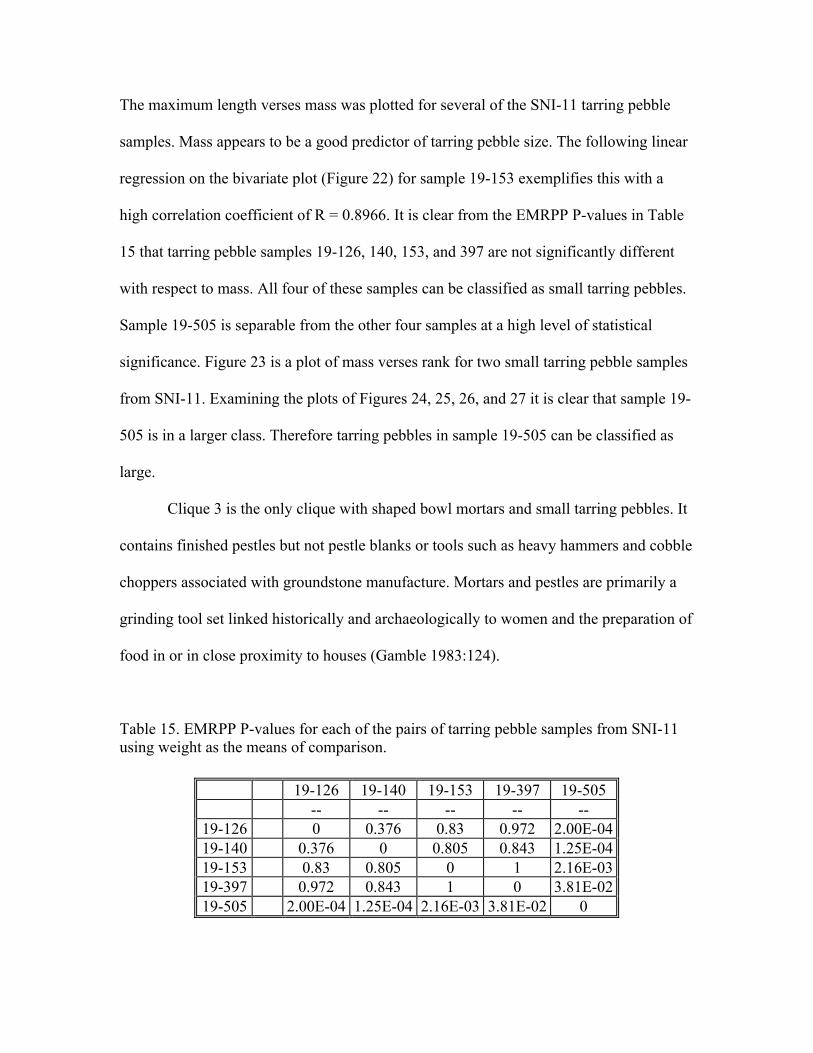
The maximum length verses mass was plotted for several of the SNI-11 tarring pebble

samples. Mass appears to be a good predictor of tarring pebble size. The following linear

regression on the bivariate plot (Figure 22) for sample 19-153 exemplifies this with a

high correlation coefficient of R = 0.8966. It is clear from the EMRPP P-values in Table

15 that tarring pebble samples 19-126, 140, 153, and 397 are not significantly different

with respect to mass. All four of these samples can be classified as small tarring pebbles.

Sample 19-505 is separable from the other four samples at a high level of statistical

significance. Figure 23 is a plot of mass verses rank for two small tarring pebble samples

from SNI-11. Examining the plots of Figures 24, 25, 26, and 27 it is clear that sample 19-

505 is in a larger class. Therefore tarring pebbles in sample 19-505 can be classified as

large.

Clique 3 is the only clique with shaped bowl mortars and small tarring pebbles. It

contains finished pestles but not pestle blanks or tools such as heavy hammers and cobble

choppers associated with groundstone manufacture. Mortars and pestles are primarily a

grinding tool set linked historically and archaeologically to women and the preparation of

food in or in close proximity to houses (Gamble 1983:124).

Table 15. EMRPP P-values for each of the pairs of tarring pebble samples from SNI-11 using weight as the means of comparison.

19-126 19-140 19-153 19-397 19-505 -- -- -- -- --

19-126 0 0.376 0.83 0.972 2.00E-04 19-140 0.376 0 0.805 0.843 1.25E-04 19-153 0.83 0.805 0 1 2.16E-03 19-397 0.972 0.843 1 0 3.81E-02 19-505 2.00E-04 1.25E-04 2.16E-03 3.81E-02 0

Figure 22. Tarring pebble maximum length verses mass.

Figure 23. Plot of the mass of two samples of small tarring pebbles from SNI-11.

Figure 24. Plot of the mass of a sample of small and large tarring pebbles from SNI-11.

Figure 25. Plot of the mass of a sample of small and large tarring pebbles from SNI-11.

Figure 26. Plot of the mass of a sample of small and large tarring pebbles from SNI-11.

Figure 27. Plot of the mass of a sample of small and large tarring pebbles from SNI-11.

Clique 3 also contains notched cobbles and fishhook drills. As was discussed earlier it is

plausible that some of the notched cobbles in the Pitas Point sample may have been used

in the processing of plant materials and not as net weights. It is also possible that net

weights were stored in household kitchen areas. The presence of fishhook drills and the

absence of fishhook blanks on Clique 3 may indicate that fishhook drills were stored in

the kitchen areas of houses as well. Based on these observations Clique 3 appears to be a

kitchen area household tool kit used in the preparation of food and the manufacture of

small water bottles. The small water bottle or ‘us’em is described by Hudson and

Blackburn (1983:39) as:

A twined, asphaltum-covered basket with a narrow neck and rounded body, used for holding water.

Craig (1967:97-99) summarizes Harrington’s ethnographic data on the dimensions of the

small water bottle as: eighteen inches in height, eleven inches in diameter, with a mouth

about two inches across (Figure 28). It is apparent based on the counts in Table 9 that at

Pitas Point small water bottles were manufactured primarily within Areas 1 and 3. The

focus in the manufacture of small water bottles in Areas 1 and 3 and larger water bottles

in other areas in VEN-27 may be attributable to both craft specialization and function.

Small water bottles may have functioned primarily as canteens to carry water when away

from camp, whereas larger bottles may have been used to store water in the camp.

Clique 4 is also interpreted as a household tool kit. It is the only clique with

asphaltum applicators. Clique 4 also contains cobble choppers, pestle blanks, and large

tarring pebbles. Clearly this clique is connected to the manufacture of large water bottles,

Asphaltum applicators may have been used in the manufacture of a variety of basket

types. Cobble choppers could have been used in conjunction with asphaltum applicators

in the manufacture of these baskets. Choppers as already suggested could have been used

to cut the fibers. (Gamble 1983:127) cites parching trays, the X’i’m or storage basket,

and the patsmu or boiling basket as types of baskets the Chumash often applied

asphaltum to. The asphaltum applicator appears to be the tool of choice for this particular

task. For example, the X’i’m or storage basket often had asphaltum applied to its base

since the basket was typically placed on dirt areas inside houses (C. King 2003, personal

communication). Clique 4 also contains pestle blanks and cobble choppers. It appears that

cobble choppers were used in the manufacture of groundstone tools and here possibly in

the manufacture of pestles. This assertion is supported by ethnographic studies in the

Mayan Highlands (Hayden and Nelson 1981).

Toolkits and Activity Areas in SNI-25

Methods of Analysis

EMRPP and Network Analysis

As discussed previously the P-values of the EMRPP deltas as used in this thesis

provide a precise measure of the pair wise spatial association of surface artifact types

within the SNI-25 sampling area. Here a

!

" P-value

!

" 0.05 provides a statistically

significant measure that a pair of artifact types in the SNI-25 sampling area is not

spatially associated. Table 16 lists the surface artifact types in the SNI-25 sampling area

by number. Table 17 is the matrix constructed with the EMRPP

!

" P-values

corresponding to pairs of artifact types in Table 16. Table 18 is the adjacency matrix

resulting from the binary coding of the

!

" P-values in Table 17. As was discussed earlier a

1 in the adjacency matrix represents a spatial relationship between two artifact types and

a 0 represents a lack of such a relationship. Figure 25 is the network graph resulting from

the adjacency matrix (Table 18). The cliques of the network graph (Figure 29 and Table

19) are interpreted as surface artifact associations or toolkits linked to specific activity

area types in SNI-25.

Table 16. SNI-25 surface artifact types used in the EMRPP.

# Surface Artifact Type 1 Chopper 2 Chopper/Hammer 3 Core 4 Cortex-Based Scraper 5 Scraper 6 Mortar Fragment 7 Core Fragment 8 Quartzite Flake 9 Metavolcanic Flake

Table 17.

!

" P-value matrix constructed using the results of the EMRPP used for the pairwise comparison of the spatial distribution of nine surface artifact types in the sampling area of SNI-25.

1 2 3 4 5 6 7 8 9 -- -- -- -- -- -- -- -- -- 1 0 0.584915 0.157842 0.799001 0.781818 0.277577 0.493689 0.096066 0.051905 2 0.584915 0 0.634921 0.582251 0.642857 0.146187 0.49794 0.063131 0.019094 3 0.157842 0.634921 0 0.41342 0.309524 0.031635 0.138965 0.029040 0.002468 4 0.799001 0.582251 0.41342 0 0.971429 0.439311 0.838074 0.199883 0.227485 5 0.781818 0.642857 0.309524 0.971429 0 0.56044 0.821245 0.412121 0.496901 6 0.277577 0.146187 0.031635 0.439311 0.56044 0 0.423987 0.402406 0.260381 7 0.493689 0.49794 0.138965 0.838074 0.821245 0.423987 0 0.150578 0.079734 8 0.096066 0.063131 0.029040 0.199883 0.412121 0.402406 0.150578 0 0.603955 9 0.051905 0.019094 0.002468 0.227485 0.496901 0.260381 0.079734 0.603955 0

Table 18. Adjacency matrix resulting from the binary coding of the EMRPP

!

" P-values in Table 17 using a cut-off of 0.05.

Table 19. Resulting cliques that are interpreted as either house or outdoor tool kits in SNI-25.

1 2 3 4 5 6 7 8 9 -- -- -- -- -- -- -- -- -- 1 0 1 1 1 1 1 1 1 1 2 1 0 1 1 1 1 1 1 0 3 1 1 0 1 1 0 1 0 0 4 1 1 1 0 1 1 1 1 1 5 1 1 1 1 0 1 1 1 1 6 1 1 0 1 1 0 1 1 1 7 1 1 1 1 1 1 0 1 1 8 1 1 0 1 1 1 1 0 1 9 1 0 0 1 1 1 1 1 0

Clique 1 Clique 2 Clique 3 Choppers Choppers Choppers Chopper/Hammers Cortex-Based Scrapers Chopper/Hammers Cortex-Based Scrapers Scrapers Cores* Scrapers Mortar Fragments Cortex-Based Scrapers Mortar Fragments Core Fragments Scrapers Core Fragments Quartzite Flakes Core Fragments Quartzite Flakes Metavolcanic Flakes*

Figure 29. Network graph of SNI-25 surface artifact associations resulting from a cut-off of 0.05 for the EMRPP P-values in Table 17.

Interpretation of Results

Outdoor Activity Area Toolkits in the SNI-25 Sample

Clique 3 is interpreted as an outdoor activity area tool kit because it is the only

clique that does not contain mortar fragments. As discussed in a previous section the

manufacture and use of groundstone tools is strongly linked to house areas over a wide

geographic area in the Americas. It is likely that the artifact association in Clique 3 is part

of one or more larger outdoor activity area tool kit(s) in SNI-25. The missing artifact

types in the complete outdoor activity area tool kit(s) of which Clique 3 is likely a part

could be discovered through either increasing the size of the site surface sampled or from

a separate analysis of typed artifacts recovered in the ongoing excavation at SNI-25.

Some of the missing artifact types could also be predicted using the results from the

analysis in this thesis of typed artifact counts from four excavated areas in VEN-27.

Clique 3 contains choppers, chopper/hammers, cortex-based scrapers, scrapers, and core

fragments. These stone artifacts were likely used either individually or in different

combinations for a myriad of tasks. All the stone artifacts in Clique 3 could have been

used together in wood working activities such as in the construction of watercraft.

Several of the cortex-based scrapers in the SNI-25 sample look quite similar to scraper

planes and possibly were used for the same purposes. This, along with their large size,

suggests that cortex-based scrapers in SNI-25 may have frequently been used to plane

driftwood into planks. Such planks were required for the construction and repair of wood

plank canoes. Scraping tools in general (including scraper planes) may also have been

used together in the carving of wooden objects such as driftwood bowls and utensils and

again in the separation of plant fibers for weaving baskets. Depending on the plant source

cortex-based scrapers at SNI-25 may also have been used to separate plant fibers made

into cordage, nets, and fishing line. Small cobble chopper/hammers and core fragments

might have been used as light hammers in the initial breaking of shell used to

manufacture utilitarian objects, ornaments, and beads.

Flake Use in SNI-25 Outdoor Activity Areas

A common choice for testing 2-sample data of the type in Table 20 is the t-test.

This would be a poor choice for archaeological data since it assumes normality of the

single-response variables (here the lengths of woodworking flakes and butchering flakes

are grouped into six length classes). Also the t-test is a variance-based statistic, and is

therefore sensitive to outlying data observations. A much better choice for analyzing the

data is a robust non-parametric statistic, adjusted specifically for 2-sample data. A MRRP

adjusted for 2-sample data is such a statistic, and therefore requires no a priori

assumptions about the distributions of the single response variables. Also the MRPP as

applied to the data in Table 20, uses absolute deviations, which are far less sensitive to

outlying values in data than the squared measures used in variance-based statistics. The

raw data in Table 20 was entered into the blossom software as an ASCII file in the format

of Table 21. The commands used to implement the MRPP analysis are given in Table 22.

The results of the MRPP are given in Table 23. The P-value is approximately 0.05, which

is significant at the five percent level. This indicates that the two samples are likely from

different populations, which substantiates the use of flake length to distinguish a sample

of woodworking flakes from a sample of butchering flakes. Figure 30 is a plot of the

flake lengths in Table 20.

Table 20. Adapted from (Keeley 1980:112). Relationship between use and flake length resulting from experiments using replicated flakes. Values in the table are counts of flakes in each of six length categories.

Use Flake Length < 4 cm 4-4.9 cm 5-5.9 cm 6-6.9 cm 7-7.9 cm > 8 cm

Woodworking 4 6 2 1 4 4 Butchering 2 1 2 3 1 2

Table 21. ASCII format entered as a Notepad text (*.txt) file into the Blossom software to test for the equality of medians of the data in Table 20, using MRPP with absolute deviations (Euclidean distance).

GROUP RESPONSE 1 4 1 6 1 2 1 1 1 4 1 4 2 2 2 1 2 2 2 3 2 1 2 2

Prior to discussing the uses of quartzite and metavolcanic flakes in outdoor

activity areas in SNI-25 it should be noted that within activity areas in the SNI-25

sampling area metavolcanic flakes and quartzite flakes along with probable flake scrapers

made from the same material occur in dense clusters in Outdoor Activity Area #1. These

clusters are discrete and well separated from the other surface artifacts in these areas.

Also, by inspection these clusters are quite homogeneous with respect to surface artifact

type.

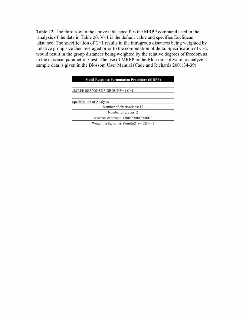
Table 22. The third row in the above table specifies the MRPP command used in the analysis of the data in Table 20. V=1 is the default value and specifies Euclidean distance. The specification of C=1 results in the intragroup distances being weighted by relative group size then averaged prior to the computation of delta. Specification of C=2 would result in the group distances being weighted by the relative degrees of freedom as in the classical parametric t-test. The use of MRPP in the Blossom software to analyze 2- sample data is given in the Blossom User Manual (Cade and Richards 2001:34-39).

Multi-Response Permutation Procedure (MRPP) >MRPP RESPONSE * GROUP/V=1 C=1 Specification of Analysis

Number of observations: 12 Number of groups: 2

Distance exponent: 1.000000000000000 Weighting factor: n(I)/sum(n(I)) = C(I) = 1

Table 23. Results of the MRPP performed on the data in Table 20.

Figure 30. Plot of the flake length frequencies corresponding to the two activity types for each of the six length classes in Table 20. Therefore it seemed reasonable not to complicate matters by including these locations in

the network analysis. In other words these flake clusters must be the remnants of a

distinct tool kit. This explains the result of the network analysis, which places

metavolcanic and quartzite flakes only in cliques interpreted as house area tool kits.

In considering the use of flakes in outdoor activity areas in SNI-25, flake length

has been suggested as a good indicator of use based on the results of replicative

Group Summary Group Value Group Size Group Distance

1 6 2.066666667 2 6 0.866666667

Results

Delta Observed = 1.466666667 Delta Expected = 1.757575758 Delta Variance = 0.020422406 Delta Skewness = -2.043237443

Standardized test statistic = -2.035653431

Probability (Pearson Type III) of a smaller or equal delta = 0.0481835593

experiments given in (Keeley 1980). This suggestion is buttressed by the results of the

preceding statistical analysis of the flake length counts in Table 20. The data in Table 20,

which is graphically depicted in Figure 30, can be used to predict that the shortest

metavolcanic flakes as well as those of greatest length were more likely used in

woodworking than for butchering in SNI-25. On San Nicolas Island driftwood is the most

easily obtained source of wood since as mentioned earlier trees and woody shrubs with

the possible exception of a willow are not native to the island. It is also likely that many

flakes in SNI-25 were used in working shell and some in the shaping of soft stone,

categories not considered in Keeley’s (1980) research.

Figure 31 is a graph of the frequency verses length of the metavolcanic flakes

belonging to several flake clusters within a 5 x 5 meter quadrat placed in Outdoor

Activity Area #1 in the SNI-25 sampling area. This plot has three peaks, which suggests a

minimum of three length classes for the metavolcanic flakes in this sample. The first peak

is centered close to 2 cm, which strongly suggests flakes in this length class were used

primarily in woodworking (Table 20 and Figure 30) and, considering the ecological

setting of San Nicolas Island, the working of shell. The second peak is close to 2.5 cm,

which also suggests flakes in this class, were most likely used in shell and woodworking.

The third peak is at 4 cm, which again points to flakes in this length class being used in

the working of shell and wood. One of the flakes in Figure 31 is 7 cm in length and is

also a sample outlier. Based on the data in Table 20 this flake was most likely used in

woodworking and possibly in shell working as well.

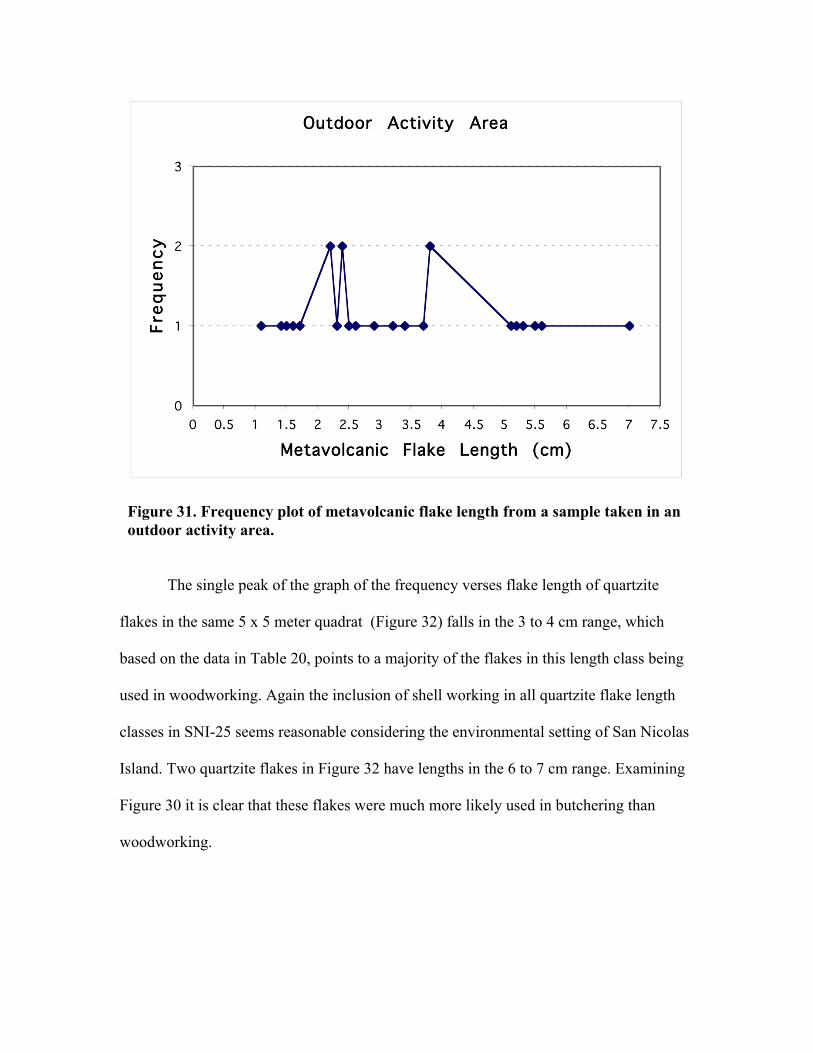
Figure 31. Frequency plot of metavolcanic flake length from a sample taken in an outdoor activity area.

The single peak of the graph of the frequency verses flake length of quartzite

flakes in the same 5 x 5 meter quadrat (Figure 32) falls in the 3 to 4 cm range, which

based on the data in Table 20, points to a majority of the flakes in this length class being

used in woodworking. Again the inclusion of shell working in all quartzite flake length

classes in SNI-25 seems reasonable considering the environmental setting of San Nicolas

Island. Two quartzite flakes in Figure 32 have lengths in the 6 to 7 cm range. Examining

Figure 30 it is clear that these flakes were much more likely used in butchering than

woodworking.

Figure 32. Frequency plot of quartzite flake length from a sample taken in an outdoor activity area.

House Activity Area Toolkits in SNI-25

In Table 19, Cliques 1 and 2 are interpreted as house activity area tool kits

because both cliques contain mortar fragments. Clique 1 also contains choppers,

chopper/hammers, cortex-based scrapers, scrapers, and quartzite flakes. As previously

discussed choppers and chopper/hammers could have been used in house activity

areas in tasks such as the chopping of wood and bone and in the manufacture of

groundstone tools. Again in SNI-25 cortex-based scrapers were likely used in

woodworking and plant fiber extraction. Scrapers are likely a multi-purpose house

activity area tool in SNI-25 and were likely used in the working of wood, bone, shell, and

soft stone. The use of flakes in SNI-25 house activity areas will be discussed shortly.

Unlike Clique 1 chopper/hammers are absent and metavolcanic flakes are included in

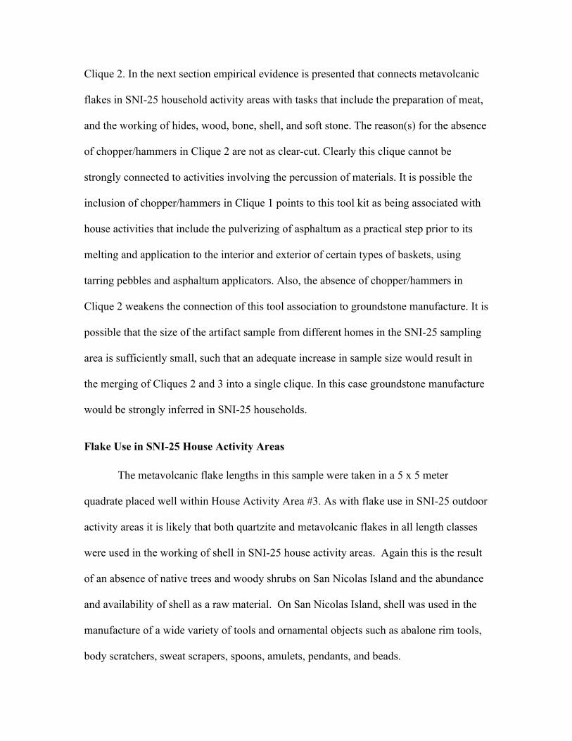
Clique 2. In the next section empirical evidence is presented that connects metavolcanic

flakes in SNI-25 household activity areas with tasks that include the preparation of meat,

and the working of hides, wood, bone, shell, and soft stone. The reason(s) for the absence

of chopper/hammers in Clique 2 are not as clear-cut. Clearly this clique cannot be

strongly connected to activities involving the percussion of materials. It is possible the

inclusion of chopper/hammers in Clique 1 points to this tool kit as being associated with

house activities that include the pulverizing of asphaltum as a practical step prior to its

melting and application to the interior and exterior of certain types of baskets, using

tarring pebbles and asphaltum applicators. Also, the absence of chopper/hammers in

Clique 2 weakens the connection of this tool association to groundstone manufacture. It is

possible that the size of the artifact sample from different homes in the SNI-25 sampling

area is sufficiently small, such that an adequate increase in sample size would result in

the merging of Cliques 2 and 3 into a single clique. In this case groundstone manufacture

would be strongly inferred in SNI-25 households.

Flake Use in SNI-25 House Activity Areas The metavolcanic flake lengths in this sample were taken in a 5 x 5 meter

quadrate placed well within House Activity Area #3. As with flake use in SNI-25 outdoor

activity areas it is likely that both quartzite and metavolcanic flakes in all length classes

were used in the working of shell in SNI-25 house activity areas. Again this is the result

of an absence of native trees and woody shrubs on San Nicolas Island and the abundance

and availability of shell as a raw material. On San Nicolas Island, shell was used in the

manufacture of a wide variety of tools and ornamental objects such as abalone rim tools,

body scratchers, sweat scrapers, spoons, amulets, pendants, and beads.

The metavolcanic flake length relative frequency plot (Figure 33) is multi-modal

with four peaks, which suggests a minimum of four length classes. The first peak in

Figure 29 is centered near 2.5 cm, which as before suggests that these flakes were more

likely used in woodworking than butchering, and again in the case of San Nicolas Island,

possibly for scraping and/or chipping shell, small bone, and soft shell. The second peak is

the largest (frequency of four) and is close to 3.5 cm, which as before, suggests flakes in

this class were most likely used in the working of shell and wood. The third peak occurs

at 3.6 cm and is bounded by 3.5 and 3.7 centimeters, which suggests flakes in this class,

were most likely used in wood and shell working, again based on the data in Table 20 and

the abundance of shellfish in the rocky inter-tidal and near shore areas of San Nicolas

Island. Five metavolcanic flakes in Figure 33 have lengths between 5 and 6 cm. Looking

at Figure 30 and Table 20 it is apparent that it is equally likely that these flakes were used

in either woodworking or butchering. Again, the ecological setting of San Nicolas Island

suggests these flakes were also probably used in the working of shell, small bone and soft

stone. In fact a feature that appears to be an Olivella biplicata shell bead and fishhook

(abalone and Norris top snail) manufacturing tool kit was recently recovered at one site

on San Nicolas Island (CA-SNI-160) and is discussed in detail in (Rosenthal, et al. 1998).

The feature is a twined sea grass bag filled with shells and tools. Of interest here, the bag

contained seven metavolcanic flakes from 0.5 to 5 cm in length. Without having the

length measurements of all seven flakes from the CA-SNI-160 sample a frequency plot

like Figure 33 cannot be made. It is striking, nonetheless, how close the length range of

the seven metavolcanic flakes is (excluding two outlier flakes in the SNI-25 samples) to

the length range of the two metavolcanic flake samples taken, one in an interpreted house

activity area, the other in an interpreted outdoor activity area, in the SNI-25 sampling

area (Figures 31 and 33, Appendix C). This buttresses the interpreted results of the VEN-

27 analysis, which infers shell fishhook manufacturing took place in both house and

outdoor activity areas.

A single metavolcanic flake, which constitutes a statistical outlier in the house

activity area sample, has a length of 7.5 cm. It is apparent from this outlier and by

inspection of Figure 33 that household activities in SNI-25 do not seem to have required

a proportionately large number of metavolcanic flakes at the upper end of the length

range. A 7.5 cm flake was much more likely used in woodworking than in butchering as

is clear in Table 20. In Figure 34 the frequency of quartzite flake lengths in the house

activity area sample consists of only three flakes and is unimodal (one class). Also, the

quartzite flake lengths in this sample are within the 3 to 4 cm ranges, which again based

on the data in Table 20, suggests these flakes were much more likely used in

woodworking than in butchering, and (again in consideration of the scarcity of living

wood sources on San Nicolas Island and the abundance and diversity of shell along with

the availability of small bone, especially bird and fish bone) in the working of shell and

bone in SNI-25 house areas. Also, quartzite flakes in the house activity area sample

comprise only a small percentage of the total sample. This may be an indication that

quartzite flakes were used in more specialized activities in SNI-25 house activity areas

than metavolcanic flakes, or simply a consequence of quartzite being less abundant than

metavolcanics on San Nicolas Island.

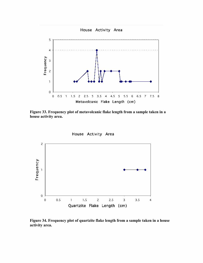
Figure 33. Frequency plot of metavolcanic flake length from a sample taken in a house activity area.

Figure 34. Frequency plot of quartzite flake length from a sample taken in a house activity area.

Finally, the multimodality of Figure 33 is evidentiary of the multi-use and size

selected nature of metavolcanic flakes in SNI-25 house activity areas. The absence of

metavolcanic flakes in Clique 1 therefore suggests this is a tool kit not as strongly tied to

butchering, and the working of wood, shell, bone, and soft stone in SNI-25 household

areas as the tool association of Clique 2.

Comparison of Tool Kits in VEN-27 and SNI-25

As was mentioned earlier, the full range of the 21 artifact types in the VEN-27

sample is found in SNI-25, with some minor intersite differences in material and

morphology for some of these artifact types. For example, fishhooks and fishhook blanks

at SNI-25 are made from Red Abalone (Haliotis rufescens) and Norris’ Top Snail

(Norrisia norrisi), whereas the fishhooks from the Pitas Point (VEN-27) excavation are

all made from California mussel (Mytilus californianus). This is likely the result of a very

small or non-existent standing stock of Haliotis rufescens as well as Norrisia norrisi in

the waters off Pitas Point throughout the time of its occupation. The similarities in time of

occupation, environmental location, and composition of artifact assemblage suggest that

some equivalent artifact associations exist in both sites. For example it is expected that as

in VEN-27 shell fishhooks at SNI-25 were manufactured using a tool kit that included

drills.

In both SNI-25 and VEN-27 the results of rigorous mathematical analyses infer

that the morphologically similar cortex-based scrapers (SNI-25) and domed scrapers

(VEN-27) belong to tool kits in both house and outdoor activity areas. As was discussed

earlier one possible use of domed (VEN-27) and cortex-based (SNI-25) scrapers is in the

manufacture and repair of wood plank canoes. Comparison of coast and interior sites

could help test the association of these two types of scraper with wood plank canoes.

Another inferred similarity in the artifact associations of VEN-27 and SNI-25 is the

inclusion of meat cutting/butchery “flakes” in SNI-25 and the functionally equivalent

“flake knives” in VEN-27 in both outdoor and house activity area tool kits. A major

difference between the two sites is the inclusion of cores in both outdoor and house

activity area tool kits (Cliques 1, 2, and 3) in VEN-27 and the statistically significant lack

of spatial association of this artifact type with house activity areas in the area sampled in

SNI-25. One obvious partial explanation for this difference is that core reduction and the

use of cores, as tools did not occur to a large extent in SNI-25 house activity areas.

Another noteworthy difference between the two sites is the spatial association of

choppers with mortars in SNI-25 and the weaker association of these two artifact types in

VEN-27. As mentioned earlier, a fairly recent ethnographic study in the Mayan

Highlands connects choppers to groundstone manufacture (Hayden and Nelson 1981).

This suggests mortars probably were manufactured at SNI-25 in house activity areas.

Conclusion

The purpose of this study was to identify and explain spatial organization of

surficial artifact distributions in CA-SNI-25 and to compare this organization against

hypothesized types of activities in order to accept or reject the hypotheses. This thesis

departs from previous research into the organization of prehistoric southern California

village sites in that sophisticated quantitative procedures are used to analyze spatial and

material data. Previous researchers have by and large analyzed site organization using

traditional and descriptive archaeological methods whereby cultural materials are

associated with features and stratigraphic lenses (Gamble 1991). Examples of southern

California sites studied in this manner are Pitas Point (Gamble 1983), Talepop (King et

al. 1982), Spring Canyon (King et al. 1989), and Oak Park (King et al.1991). All of the

spatial data generated in these studies are amendable to re-analysis using the novel

methods introduced in this thesis. A comparative study of these data using the

quantitative methods presented in this thesis would significantly add to the knowledge of

the organization of human societies.

Significant contributions to the knowledge of past human behavior have resulted

from the intrasite spatial analyses performed in this thesis. What are interpreted as four

house activity areas and two outdoor activity areas were discovered within SNI-25 using

the Clark and Evans nearest neighbor statistic in combination with approximate sampling

distributions obtained from Monte Carlo simulations (Chapter 3). The Clark and Evans

nearest neighbor analysis as used in this thesis demonstrates that the locations of houses

and other areas of organized activity in an archaeological site can be strongly inferred

using a straightforward quantitative method which requires only the provenience and

typing of surface artifacts. The Clark and Evans nearest neighbor method is a powerful

and efficient analytical tool in the elucidation of the internal organization of an

archaeological site. The predictions (e.g. locations of houses) of such an analysis would

be of significant economic value in the planning stage of an archaeological excavation,

when the placement and number of units are considered in relation to the research design

and goals.

One of the conclusions from the nearest neighbor analysis is that there is a dense

cluster of three houses at the northern edge of SNI-25. Dense house clustering has been

observed in Chumash villages (Gamble 1991). This adds to the evidence that SNI-25 was

a substantial habitation site. It is noteworthy that the north edge of SNI-25 affords the

best view of the nearby northern shoreline of San Nicolas Island, where SNI-25

watercraft such as wooden canoes may have been kept.

The results of the analyses conducted in this thesis provide objective evidence that

several of the hypothesized activity area types exist in SNI-25, as well as at a mainland

village site, VEN-27. These hypothesized activity area types fall into two larger

categories, house and outdoor activity areas. Three house activity area types are inferred

from these analyses for both SNI-25 and VEN-27. These include areas where food was

prepared (Type 2a Areas) and cooked (Type 2b Areas), and where groundstone was

manufactured (Type 2c Areas). The co-occurrence of pestle blanks, shaped pestles, and

choppers in Clique 1 of the VEN-27 network graph strongly infers that groundstone tools

were manufactured in household activity areas in this site. It has been suggested in a

previous study (Gamble 1991) that some of the pestles produced at VEN-27 were traded.

Clique 3 of the SNI-25 network graph associates mortar fragments and choppers in this

site. Other research provides evidence for mortar and pestle manufacturing on Santa Cruz

and San Miguel Island (King 1976: 314; Rozaire 1983; Walker and Snethkamp 1984).

However, the degree to which groundstone tools were manufactured in village household

activity areas in prehistoric southern California remains an important research question.

The ethnographic data provided by Hayden and Nelson (1981) identifies men as

manufacturing groundstone tools in activity areas outside of villages and close to the raw

material sources. As discussed in an earlier section, choppers are used for pecking in the

manufacture of groundstone tools.

The analysis of the quartzite and metavolcanic flake length (Chapter 3) from

clusters within the SNI-25 sampling area, in combination with the empirical information

of Keeley (1980) relating flake length to function, provides an objective basis for

inferring the presence of Type 1b Areas within SNI-25 where butchering of fish and

marine mammals took place and Type 1c Areas where wood, bone, and shell tools were

manufactured. Flake clusters are present in both the inferred SNI-25 house and outdoor

activity areas, but are larger and more homogeneous with respect to other artifact types in

the two outdoor activity areas. Ethnography connects woodworking and butchering

strongly to men, and the distribution and size of surface flake clusters in SNI-25 connects

these activity area types most strongly to outdoor areas. The presence of activity areas

within SNI-25 where fishing equipment was manufactured and repaired (Type1a Areas)

and where baskets, bone awls, and asphaltum containers were manufactured (Type 2d

Areas) could not be inferred by this intrasite spatial analysis. This is because artifacts

used in these activities were not observed in the sampling area. With respect to Type1a

Areas others and myself observed several Red Abalone and Norris Top Snail fishhooks

and fishhook blanks just outside the sample area, as well as in other areas of the site. It is

almost certain that shell fishhooks and fishhook blanks are present in the SNI-25 sample

area, but are less common or not as apparent as the stone artifacts on the surface of the

site in this area.

Tarring pebbles and asphaltum are quite common in SNI-25 and are indicative of

production activities in Chumash villages and settlements (Gamble 1991). However, no

tarring pebbles were observed in the sample area. A larger sample area and more time in

the field would assuredly have provided the location based samples of tarring pebbles and

asphaltum needed to make an objective case for inferring the manufacture of asphaltum

coated baskets at SNI-25 in specific types of activity areas.

In sum, the mathematical techniques presented in this thesis could be used to

identify activity areas and tool associations in many archaeological sites in southern

California and elsewhere. A comparative study of the results of several such analyses

applied to interior and coastal southern California sites would aid in the formulation and

testing of broad research questions and hypotheses pertaining to the structure, function,

and variability of the social systems and subsystems in these and all human societies.

CHAPTER 4

SUMMARY, CONCLUSIONS AND RECOMMENDATIONS FOR

FUTURE RESEARCH

Summary and Conclusions

The analytical methods used in thesis are both rigorous and objective. The

mathematical techniques applied to this end are appropriate, powerful, and elegant. Some

of the mathematical techniques that were applied in this thesis to study the internal

organization of SNI-25 and to discover tool kits are new to California archaeology. The

importance of using appropriate methods to study structural patterns within

archaeological sites is articulated as follows:

Archaeological techniques developed to study the internal organization of sites are critical since they provide a means of increasing knowledge of societies throughout the world [King 2000: 90]. More than anything else it is hoped that this thesis will inspire present and future

students of California prehistory to embrace advanced mathematical methods in their

research endeavors.

Recommendations for Future Research

Population Dynamics

Knowledge of the internal organization of a site can be used as a starting point in

predicting the population size of a hunter-gather community at different points in time.

Changes in population size over time can in turn be used to reconstruct the population

dynamics of a site if the number and location of contemporaneous houses is known

within one or more sub areas of a site. Population size for a specific period of time in a

sub area (or sampling area) of a hunter-gather site can be estimated using the area (here

called “camp area”) of the smallest circle that encloses all houses of equivalent age in a

sampling area. An allometric model as a means of estimating population from “camp

area” in hunter-gatherer camps is developed and tested in Wiessner (1974) with very

favorable results. This model is applicable to SNI-25 or any other hunter-gatherer

residential site for that matter. An allometric model derives from the law of allometric

growth, which states, “the rate of relative growth of an organism is a constant fraction of

the growth of the total organism” (Nordbeck 1971: 54). The underlying assumptions of

Wiessner’s model are: (1) all hunter- gather camps have the same form (shape) of

population distribution; and (2) Nordbeck’s derivation b-value in the allometric growth

formula ! = ! ∗ !! (! equals area, ! equals population) is applicable to hunter-gatherer

populations. Wiessner determined that for hunter-gather camps the denominator of the b-

value (which represents settlement dimensionality) is 1 and that the numerator (a constant

dimension of area) for hunter-gather camps is 2. Therefore a theoretical b-value of 2 was

shown to be applicable to hunter-gatherer camps. Taking the natural logarithm of both

sides of the equation provides a linear equation of the form !" ! = 1! ∗ !" ! −

!" ! . A linear regression on a !" scatter plot log of “camp area” (y-axis) to log of

camp population (x-axis) can then be used to estimate ! and.!. Wiessner used !Kung

Bushmen data to fit the model. The regression resulted in a high correlation coefficient of

0.91 and a measured b-value (slope of the regression line) of 1.96, which is very close to

the theoretical value of 2. The estimated value of !" ! was −0.23± 0.68, which is close

to zero. Using a rough estimate of camp area as ! ∗ 11! ≈ 380.1 square meters for

House Activity Areas #1, 2, and 3 in the SNI-25 sampling area, the above equation yields

! ≈ !!!∗ !"  (!"#.! !!.!") ≈ !!.!" ≈ 21.9 persons total occupying the three house activity

areas. This averages to approximately seven persons per household.

Energy Flow and Storage Knowledge of the internal organization of a site can also be used to construct

energy systems models that can be used to predict energy flow and storage patterns

within a site. Data obtained from replicative experiments can be used to calibrate the

constants of energy flow and storage equations that model the energetics of one or more

of the activities believed to have occurred within an activity area. Ethnographic data from

studies of recent maritime-based hunter-gatherer societies could also conceivably be used

as an alternative to estimate the constants of energy flow and storage equations.

Following the estimation of the energy flow and storage equation constants, computer

simulations could then be implemented to study the energetics of specific types of

organized activities, under a variety of different conditions. It is posited here that energy

based systems models (e.g. Figure 35) operationalized with computer simulation are

needed in the attempt to understand activity areas in a prehistoric archaeological site.

Figure 35. Energy flow and storage diagram depicting a possible subsystem in SNI-25. This system can be simulated on a computer using the Extend software, following the empirical determination of the model parameters.

For example, the energy flow and storage rates resulting from the procurement and

processing of Red Maids seeds (using mortars and pestles) at SNI-25 as well as the trade

of this annual seed to mainland locations in exchange for valuable and nutritious

perennial seeds (e.g. acorns and cherry pits) could then be predicted using the following

energy systems model once the model parameters have been estimated (Figure 35).

Refer to (Odum and Odum 2000) for the mathematical definitions of the symbols used in

this model and for its simulation using Extend LT, which is provided on a CD ROM that

comes with the book. Once fully operationalized this energy system model in

combination with a population estimate of SNI-25 will objectively predict the relative

importance of a local seed crop in the subsistence and trade economy of the site’s

inhabitants under a number of different scenarios.

REFERENCES CITED Berry, K.J. 1982 Algorithm AS 179: enumeration of all permutations of multi-sets with fixed repetition numbers. Applied Statistics 31:169-173. Berry, K.J., K.L. Kvamme and P.W. Mielke 1980 A Permutation Technique for the Spatial Analysis of the Distribution of Artifacts into Classes. American Antiquity 45(1): 55-59. 1983 Improvements in the Permutation Test for the Spatial Analysis of the Distribution of Artifacts into Classes. American Antiquity 48(3): 547-553. Berry, K.J. and P.W. Mielke 1984 Computation of exact probability values for multi-response permutation procedures. Communications in Statistics --- Simulation and Computation 13: 417-432. Berry. K.J, P.W. Mielke and K.L. Kvamme 1984 Efficient Permutation Procedures for Analysis of Artifact Distributions. In Intrasite Spatial Analysis in Archaeology, edited by H.J. Hietala, pp. 54-74. Cambridge University Press, New York. Besag, J.and P.J. Diggle

1977 Simple Monte Carlo Tests for Spatial Pattern. Applied Statistics 26(3): 327-333.

Borgatti, S.P., Everett, M.G. and L.C. Freeman 2002 Ucinet for Windows: Software for Social Network Analysis. Analytic Technologies. Harvard, Massachusetts. Bron, C. and J. Kerbosch

1973 Finding All Cliques of an Undirected Graph. Communications of the ACM 16: 575-577.

Bryan, B.

1970 Archaeological Explorations on San Nicolas Island. Southwest Museum Papers No. 22. Southwest Museum, Los Angeles.

Cade, B.S. and J.D. Richards 2001 User Manual for Blossom Statistical Software. PDF file that accompanies the

software. Mid-continent Ecological Science Center. Fort Collins, Colorado. California Coastal Commission

1987 California Coastal Resource Guide. University of California Press. Berkeley, California.

Christenson, A. and D.W. Read. 1977 Numerical Taxonomy, R-Mode Factor Analysis and Archaeological Classification. American Antiquity 42:163-179. Clark, P.J. and F.C. Evans. 1954 Distance to Nearest Neighbor as a Measure of Spatial Relationships in Populations. Ecology 35(4): 445-453. Collins, P. 1982 Origin and Differentiation of the Island Fox: A Study of Evolution in Insular Populations. Masters Thesis, Department of Zoology, University of California, Santa Barbara. Craig, S. 1967 The Basketry of the Ventureno Chumash. UCLA Archaeological Survey Annual Reports 8: 201-214. Los Angeles, California. Earle, T. K. 1976 A Nearest-Neighbor Analysis of Two Formative Settlement Systems. In The Early Mesoamerican Village, edited by, K V. Flannery, pp. 196-223. Academic Press, New York. Eastwood, A.

1924 Archibald Menzies’ Journal of the Vancouver Expedition. California Historical Society Quarterly 2(4): 264-340.

Eddington, E. S.

1969 Statistical Inference: The Distribution -free Approach. McGraw-Hill, New York.

Flannery, K.V. 1976 The Early Mesoamerican Village. Academic Press, New York. Flannery, K.V. and M. C. Winter

1976 Analyzing Household Activities. In The Early Mesoamerican Village, edited by K.V. Flannery, pp. 34-47. Academic Press, New York.

Foreman, R.E. 1967 Observations of the Flora and Ecology of San Nicolas Island. United States Navy Radiological Defense Laboratory TR-67-8. Gamble, L. C. 1983 The Organization of Artifacts, Features, and Activities at Pitas Point: A Coastal Chumash Village. Journal of California and Great Basin Anthropology 5 (1& 2):103-129.

1991 Organization of Activities at the Historic Settlement of Helo’: A Chumash Political, Economic, and Religious Center. Unpublished Ph.D. dissertation, Department of Anthropology. University of California, Santa Barbara. Gauch, H.G. 1982 Noise Reduction By Eigenvector Ordination. Ecology 63(6): 1643-1649. Gifford-Gonzalez, D.P., Damrosch, D.B., Damrosch, D.R., Pryor, J., and R.L. Thunen. 1985 The Third Dimension in Site Structure: An Experiment in Trampling and Vertical Dispersal. American Antiquity 50: 803-818. Gross J. and J. Yellen 1999 Graph Theory and its Applications. CRC Press, New York. Hamy, E. 1963 The Fishhook Industry of the Ancient Inhabitants of the Archipelago of California. Reports of the University of California Archaeological Survey 59:61-69. Berkeley, California. Harary, F. and M.F. Batell 1981 What is a System? Social Networks 3: 29-40. Harary, F. and I.C. Ross.

1957 A Procedure for Clique Detection Using the Group Matrix. Sociometry 20: 205- 215.

Hayden, B. and M. Nelson 1981 The Use of Chipped Lithic Material in the Contemporary Mayan Highlands. American Antiquity 46(4): 885-898. Heizer, R.L.

1955 California Indian Linguistic Records: The Mission Indian Vocabularies of H.W. Henshaw. University of California Anthropological Records 15(2). Berkeley, California.

Hietala, H.J. and D.E. Stevens. 1977 Spatial Analysis: Multiple Procedures in Pattern Recognition Studies. American Antiquity 42(4): 539-559. Hodder I. and M. Hassall 1971 The non-random spacing of Romano-British walled towns. Man 6: 391-407. Hodson, F.R., Sneath, P.H.A., and J.E. Doran 1966 Some Experiments in the Numerical Analysis of Archaeological Data. Biometrika 53(3): 311-324.

Hoover, R. L. 1973 Chumash Fishing Equipment. San Diego Museum of Man Ethnic Technology Notes No. 9. San Diego, California. Hudson, T. and T.C. Blackburn 1979 The Material Culture of the Chumash Interaction Sphere. Volume I: Food Procurement and Transportation. A Ballena Press/ Santa Barbara Museum of Natural History Cooperative Publication. Los Altos and Santa Barbara, California. 1983 The Material Culture of the Chumash Interaction Sphere. Volume II: Food Preparation and Shelter. A Ballena Press/ Santa Barbara Museum of Natural History Cooperative Publication. Los Altos and Santa Barbara, California. 1986 The Material Culture of the Chumash Interaction Sphere. Volume V: Manufacturing Processes, Metrology, and Trade. A Ballena Press/ Santa Barbara Museum of Natural History Cooperative Publication. Menlo Park and Santa Barbara, California. Keeley, L.H. 1980 Experimental Determination of Stone Tool Uses, A Microwear Analysis. University of Chicago Press, Chicago. Kent, S. 1984 Analyzing Activity Areas: An Ethnoarchaeological Study of the Use of Space. University of New Mexico Press, Albuquerque. King, C.

1976 Chumash Intervillage Economic Exchange. In Native Californians: A Theoretical Retrospective, edited by L.J. Bean and T.C. Blackburn, pp. 289-318. Ballena Press. Ramona, California.

1990 Evolution of Chumash Society. A Comparative Study of Artifacts Used for Social System Maintenance in the Santa Barbara Channel Region before A.D.1804.

Garland Publishing Inc. New York. 2000 Native American Cultural Sites in the Santa Monica Mountains. Prepared for the Santa Monica Mountains and Seashore Foundation. King, C., W.W. Bloomer, E. Clingen, B.E. Edberg, L.H. Gamble, J.E. Hammett, J.R. Johnson, T. H. Kemperman, C.D. Pierce, and E. Wohlgemuth 1982 Archaeological Investigations at Talepop (LAn-229). Office of Public Archaeology, Social Process research Institute, University of California, Santa Barbara.

King, C., J. A. Parsons, and R.O. Gibson 1989 Space Transportation System Natural Gas Pipeline and SLC-4 Security Fence Treatment Programs, Vandenberg Air Force Base, California, Technical Reports Volumes 1A and 1B. Environmental Solutions, Inc. Irvine, California. King, C., J. Triem, J. Parsons, N. Anakouchine, B. Texier, L. Cummings, and M. Alexander 1991 Oak Park Zone III, Phase II, Archaeological Resources Assessment. Edited by C. King. Topanga Anthropological Consultants, Topanga. Submitted to First City Communities. Beverly Hills, California. Kroll, E. M. and T.D. Price (Eds.)

1991 The Interpretation of Archaeological Spatial Patterning. Plenum Press, New York.

Luce, R. and A. Perry 1949 A Method of Matrix Analysis of Group Structure. Psychometrika 14: 95-116. Marriot, F.H.C.

1978 Barnard’s Monte Carlo Tests: How many simulations? Applied Statistics 28(1): 75-77

Martz, P. 2002 San Nicolas Island Prehistoric Archaeological Sites Mapping and Recordation Project. Prepared for Naval Air Weapons Station China Lake, California Meighan, C.W. and H, Eberhart

1953 Archaeological Resources of San Nicolas Island, California. American Antiquity 19:109-125.

Merrill, M.

2002 A Spatial Analysis of Mapped Surface Artifacts from Several Early Period Sites in Los Angeles and Ventura Counties. Paper prepared for Topanga

Anthropological Consultants. Topanga, California Mielke, P.W. and K.J. Berry

2001 Permutation Methods. A Distance Function Approach. Springer-Verlag, New York.

Mielke, P.J., K.J. Berry, and E.S. Johnson 1976 Multi-response Permutation Procedures for A Priori Classifications. Communications in Statistics: Theory and Methods A5 (14):1409-1424. Molitor, M. 2000 Perforated Stones from the Ledge Site. Pacific Coast Archaeological Society Quarterly 36(2): 53-59.

Nordbeck, S. 1971 Urban Allometric Growth. Geografiska Annaler 53(B-1): 54-67. Odum, H.T. 1971 Environment Power and Society. John Wiley & Sons, New York.

1996 Environmental Accounting, Emergy, and Decision Making. John Wiley and Sons, New York.

Odum H. T. and E. C. Odum.

2000 Modeling for all Scales. An Introduction to System Simulation. Academic Press, San Diego.

Odum, H.T. and N. Peterson. 1996 Simulation and Evaluation with Energy Systems Blocks. Ecological Modeling 93:155-173. Orr, P.C. 1968 Prehistory of Santa Rosa Island. Santa Barbara Museum of Natural History, Santa Barbara, California. Pilling, A.R. 1951 The Surface Archaeology of the Pecho Coast, San Luis Obispo, California. The Masterkey 25(6):196-200. Priestly, H. I. 1972 A Historical, Political, and Natural Description of California by Pedro Fages. Ballena Press. Ramona, California. Read, D.W. 1992 The Convergence Assumption: A Fatal Flaw in Clustering Algorithms. Statistics Series No.105. University of California, Los Angeles. Read, D.W. and G. Russell 1996 A Method for Taxonomic Typology Construction and an Example: Utilized Flakes. American Antiquity 61(4): 1-22. Reinman, F.M. and G.A. Lauter 1984 San Nicolas Island Cultural Resource Survey Report 3 vols. F.M. Reinman & Associates. On file, Environmental Division, NAWS. Point Mugu, California. Rencher, A.C. 1995 Methods of Multivariate Analysis. John Wiley & Sons, Inc., New York.

Rogers, D.B. 1929 Prehistoric Man of the Santa Barbara Coast. Santa Barbara Museum of Natural History. Santa Barbara, California. Rogers, M. 1930 Field Notes: 1930 Expedition to San Nicolas Island. Ms. On file, San Diego Museum of Man. Copy on file, NAS Point Mugu, California. Rosenthal, J., P. Jertberg, W.H. Bonner, and R.R. Mariani 1998 CA-SNI-160 Index Unit and Damage Area Investigations San Nicolas Island, SLAM Target, U.S. Naval Air Weapons Station, Pt. Mugu, Ventura County, County. Prepared for: The Strike System Division NAWS/NAWC Pt. Mugu and Sverdrup AEGIR/INS, Camarillo, California. Petra Resources, Inc. Irvine, California. Rozaire, C.E.

1983 Mortar and Pestle Manufacturing on San Miguel Island, California. The Masterkey 57:131-143.

Schwartz, S.J. and P. Martz 1992 An Overview of the Archaeology of San Nicolas Island, Southern California. Pacific Coast Archaeological Society Quarterly 28(4): 46-75. Tringham, R., G. Cooper, G. Odell, B Voytek, and A. Whitman

1974 Experimentation in the Formation of Edge Damage: A New Approach to Lithic Analysis. Journal of Field Archaeology 1: 171-196.

Vedder, J.G. and R.M. Norris 1963 Geology of San Nicolas Island, California. Geological Survey Professional Paper 369. United States Government Printing Office, Washington D.C. Vellanoweth, R.

1996 Subsistence, Settlement and Marine Resource Utilization at CA-SNI-161, San Nicolas Island, California. Unpublished Masters Thesis, Department of Anthropology. California State University, Los Angeles.

Wagner, H.R. 1929 Spanish Voyages to the Northwest Coast of America in the Sixteenth Century. California Historical Society Special Publication, No. 4. San Francisco, California. Walker, P.L. 1978 Butchering and Stone Tool Function. American Antiquity 13: 710-715.

Walker, P.L. and P.E. Snethkamp 1984 Archaeological Investigations on San Miguel Island. Prehistoric Adaptations to the Marine Environment, Volume 1. Office of Public Archaeology, Social Process Research Institute. University of California, Santa Barbara. Whallon, R. 1974 Spatial Analysis of Occupation Floor II: The Application of Nearest Neighbor Analysis. American Antiquity 39(1): 16-34. 1984 Unconstrained Clustering for the Analysis of Spatial Distributions in Archaeology. In Intrasite Spatial Analysis, edited by H.J. Hietala, pp. 242-277. Cambridge University Press, New York. 1990 Defining Structure in Clustering Dendrograms with Multilevel Clustering. In New Tools from Mathematical Archaeology, edited by A. Voorhips and B. Ottaway, pp.1-14. Polish Academy of Sciences Commission on Archaeology, Krakow. Wiessner, P. 1974 A Functional Estimator of Population from Floor Area. American Antiquity 39(2): 343-350. Woodard, A. 1932 Field Notes on File at the Smithsonian Institute (No. 6042- Archaeology of California). 1938 The First Ethnologists in California. The Masterkey 12:141-151.

APPENDIX A: EXCEL 4.0 MACROS

MACRO #1: Computes approximate sampling distributions for the Clark and Evans Nearest Neighbor Statistic Monte Carlo Method as Applied to the Simulation of Q Data Sets of r Pseudorandom Numbers in an N x N Quadrat Used to Compute Approximate Sampling Distributions of the Clark & Evans Nearest Neighbor Statistic. =SELECT(OFFSET(ACTIVE.CELL(),0,3)) =SET.NAME("CounterErase",0) =WHILE(OR(ACTIVE.CELL()<>"",OFFSET(ACTIVE.CELL(),0,1)<>"",OFFSET(ACTIVE.CELL(),0,2)<>"")) =FORMULA("") =SELECT(OFFSET(ACTIVE.CELL(),0,1)) =FORMULA("") =SELECT(OFFSET(ACTIVE.CELL(),0,1)) =FORMULA("") =SELECT(OFFSET(ACTIVE.CELL(),0,1)) =FORMULA("") =SELECT(OFFSET(ACTIVE.CELL(),1,-3)) =SET.NAME("CounterErase",CounterErase+1) =NEXT() =SELECT(OFFSET(ACTIVE.CELL(),-CounterErase,-2)) =INPUT("Enter the length of the sides of the square sampling window:",1) =SET.NAME("Length",B17) =INPUT("Enter the number of artifact locations within the sampling window:",1) =SET.NAME("ArtNo",B19) =INPUT("Enter the no. of iterations to be performed:",1) =SET.NAME("IterNo",B21) =SET.NAME("CounterIter",0) =WHILE(CounterIter<IterNo) =FOR("countq",1,ArtNo) =FORMULA(Length*RAND()) =SELECT(OFFSET(ACTIVE.CELL(),0,1)) =FORMULA(Length*RAND()) =SELECT(OFFSET(ACTIVE.CELL(),1,-1)) =NEXT() =SELECT(OFFSET(ACTIVE.CELL(),-ArtNo,2)) =SET.NAME("Counter",0) =FOR("counta",1,ArtNo) =OFFSET(ACTIVE.CELL(),Counter,-2) =OFFSET(ACTIVE.CELL(),Counter,-1) =FOR("countb",1,ArtNo) =OFFSET(ACTIVE.CELL(),0,-2) =OFFSET(ACTIVE.CELL(),0,-1) =SQRT((B34-B37)^2+(B35-B38)^2) =SET.NAME("D",B39) =FORMULA(D) =SELECT(OFFSET(ACTIVE.CELL(),1,0)) =NEXT() =SELECT(OFFSET(ACTIVE.CELL(),-(ArtNo-1),0)) =SET.NAME("NN",10^8) =IF(Counter=0,SET.VALUE(OFFSET(ACTIVE.CELL(),-1,0),10^8),SET.NAME("NN",OFFSET(ACTIVE.CELL(),-1,0))) =IF(NN>ACTIVE.CELL()) =SET.NAME("NN",ACTIVE.CELL()) =END.IF() =IF(AND(Counter=1,ArtNo<>2)) =SET.VALUE(ACTIVE.CELL(),10^8) =END.IF() =SET.NAME("CounterD",2) =FOR("countc",1,ArtNo-2) =SELECT(OFFSET(ACTIVE.CELL(),1,0)) =IF(AND(Counter=CounterD,ArtNo<>2))

=SET.VALUE(ACTIVE.CELL(),10^8) =END.IF() =IF(ACTIVE.CELL()<NN) =SET.NAME("NN",ACTIVE.CELL()) =END.IF() =SET.NAME("CounterD",CounterD+1) =NEXT() =SET.NAME("up",-(ArtNo-(Counter+1))) =IF(Counter<=ArtNo) =SELECT(OFFSET(ACTIVE.CELL(),up,1)) =FORMULA(NN) =SELECT(OFFSET(ACTIVE.CELL(),-Counter,-1)) =END.IF() =SET.NAME("Counter",Counter+1) =NEXT() =SELECT(OFFSET(ACTIVE.CELL(),0,1)) =SET.NAME("Sum1NN",0) =FOR("counth",1,ArtNo) =SET.NAME("Sum1NN", Sum1NN+ACTIVE.CELL()) =SELECT(OFFSET(ACTIVE.CELL(),1,0)) =NEXT() =SELECT(OFFSET(ACTIVE.CELL(),-ArtNo,0)) =Sum1NN/ArtNo =ArtNo/(B17^2) =SET.NAME("rho",B80) =2*SQRT(B80) =B79*B82 =SELECT(OFFSET(ACTIVE.CELL(),CounterIter,1)) =FORMULA(ROUND(B83,2)) =IF(CounterIter=IterNo-1) =SELECT(OFFSET(ACTIVE.CELL(),-CounterIter,1)) =4-PI() =4*PI()*rho*ArtNo =SQRT(B88/B89) =FORMULA(B90) =END.IF() =IF(CounterIter<>IterNo-1) =SELECT(OFFSET(ACTIVE.CELL(),-CounterIter,-4)) =END.IF() =SET.NAME("CounterIter",CounterIter+1) =NEXT() =RETURN()

MACRO #2: Counts sorted output from Macro #1

=SELECT(OFFSET(ACTIVE.CELL(),0,1)) =SET.NAME("CounterP",0) =WHILE(OR(ACTIVE.CELL()<>"",OFFSET(ACTIVE.CELL(),0,1)<>"")) =FORMULA("") =SELECT(OFFSET(ACTIVE.CELL(),0,1)) =FORMULA("") =SELECT(OFFSET(ACTIVE.CELL(),1,-1)) =SET.NAME("CounterP",CounterP+1) =NEXT() =SELECT(OFFSET(ACTIVE.CELL(),-CounterP,-1)) =SET.NAME("CounterT",0) =SET.NAME("CounterU",0) =INPUT("Enter min R value:",1) =SET.NAME("CurrentVal",I15) =INPUT("Enter max R value:",1) =SET.NAME("TopVal",I17) =SET.NAME("CounterS",0) =WHILE(CurrentVal<=TopVal) =SET.NAME("CounterQ",0) =WHILE(AND(OFFSET(ACTIVE.CELL(),0,-2)<=CurrentVal,OFFSET(ACTIVE.CELL(),0,-2)<>"")) =IF(OFFSET(ACTIVE.CELL(),0,-2)=CurrentVal) =SET.NAME("CounterQ",CounterQ+1) =END.IF() =SELECT(OFFSET(ACTIVE.CELL(),1,0)) =SET.NAME("CounterS",CounterS+1) =NEXT() =OFFSET(ACTIVE.CELL(),0,-2) =ABS(I29-CurrentVal) =SET.NAME("Increment",I30) =SELECT(OFFSET(ACTIVE.CELL(),-CounterS+CounterT,1)) =FORMULA(CurrentVal) =SELECT(OFFSET(ACTIVE.CELL(),0,1)) =FORMULA(CounterQ) =SELECT(OFFSET(ACTIVE.CELL(),-CounterT+CounterS,-2)) =SET.NAME("CounterT",CounterT+1) =SET.NAME("CurrentVal",CurrentVal+Increment) =NEXT() =SELECT(OFFSET(ACTIVE.CELL(),-CounterS,0)) =RETURN()

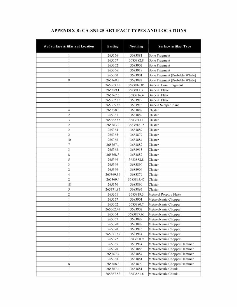
APPENDIX B: CA-SNI-25 ARTIFACT TYPES AND LOCATIONS

# of Surface Artifacts at Location Easting Northing Surface Artifact Type

1 265356 3683881 Bone Fragment 1 265357 3683882.8 Bone Fragment 1 265362 3683902 Bone Fragment 1 265366 3683919 Bone Fragment 1 265360 3683901 Bone Fragment (Probably Whale) 8 265368.3 3683882 Bone Fragment (Probably Whale) 1 265363.05 3683916.85 Breccia Core Fragment 1 265359.1 3683911.33 Breccia Flake 1 265362.6 3683916.4 Breccia Flake 1 265362.85 3683919 Breccia Flake 1 265365.65 3683913 Breccia Scraper Plane 4 265358.6 3683882 Cluster 2 265361 3683882 Cluster 3 265362.85 3683913.1 Cluster 2 265363.2 3683916.15 Cluster 2 265364 3683889 Cluster 2 265365 3683879 Cluster

10 265366 3683884 Cluster 7 265367.4 3683882 Cluster 3 265368 3683915 Cluster 8 265368.3 3683882 Cluster 5 265369 3683882.8 Cluster 3 265369 3683890 Cluster 2 265369 3683904 Cluster 4 265369.36 3683879 Cluster 2 265369.4 3683895.47 Cluster

18 265370 3683890 Cluster 5 265371.85 3683895 Cluster 2 265361 3683919.3 Metavol Porphry Flake 1 265357 3683901 Metavolcanic Chopper 1 265362 3683880.7 Metavolcanic Chopper 1 265362.47 3683902 Metavolcanic Chopper 1 265364 3683877.67 Metavolcanic Chopper 1 265367 3683889 Metavolcanic Chopper 1 265370 3683889 Metavolcanic Chopper 1 265370 3683916 Metavolcanic Chopper 1 265371.67 3683914 Metavolcanic Chopper 1 265372 3683900.9 Metavolcanic Chopper 1 265365 3683914 Metavolcanic Chopper/Hammer 1 265370 3683883 Metavolcanic Chopper/Hammer 1 265367.4 3683884 Metavolcanic Chopper/Hammer 1 265368 3683881 Metavolcanic Chopper/Hammer 8 265368.3 3683892 Metavolcanic Chopper/Hammer 1 265367.4 3683881 Metavolcanic Chunk 1 265367.52 3683881.6 Metavolcanic Chunk

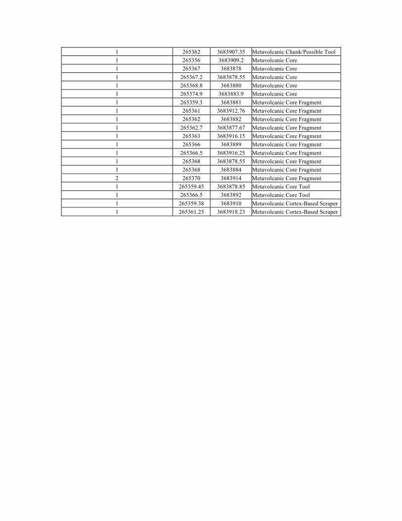
1 265362 3683907.35 Metavolcanic Chunk/Possible Tool 1 265356 3683909.2 Metavolcanic Core 1 265367 3683878 Metavolcanic Core 1 265367.2 3683878.55 Metavolcanic Core 1 265368.8 3683880 Metavolcanic Core 1 265374.9 3683883.9 Metavolcanic Core 1 265359.3 3683881 Metavolcanic Core Fragment 1 265361 3683912.76 Metavolcanic Core Fragment 1 265362 3683882 Metavolcanic Core Fragment 1 265362.7 3683877.67 Metavolcanic Core Fragment 1 265363 3683916.15 Metavolcanic Core Fragment 1 265366 3683889 Metavolcanic Core Fragment 1 265366.5 3683916.25 Metavolcanic Core Fragment 1 265368 3683878.55 Metavolcanic Core Fragment 1 265368 3683884 Metavolcanic Core Fragment 2 265370 3683914 Metavolcanic Core Fragment 1 265359.45 3683878.85 Metavolcanic Core Tool 1 265366.5 3683892 Metavolcanic Core Tool 1 265359.38 3683910 Metavolcanic Cortex-Based Scraper 1 265361.25 3683918.23 Metavolcanic Cortex-Based Scraper

1 265359.45 3683878.85 Metavolcanic Core Tool 1 265366.5 3683892 Metavolcanic Core Tool 1 265359.38 3683910 Metavolcanic Cortex-Based Scraper 1 265361.25 3683918.23 Metavolcanic Cortex-Based Scraper 1 265365 3683882.25 Metavolcanic Cortex-Based Scraper 1 265367.2 3683877 Metavolcanic Cortex-Based Scraper 1 265371 3683879.6 Metavolcanic Cortex-Based Scraper 1 265372 3683913 Metavolcanic Cortex-Based Scraper 1 265359.4 3683918.4 Metavolcanic Flake 1 265359.65 3683918.4 Metavolcanic Flake

1 265359.7 3683918.1 Metavolcanic Flake

1 265359.75 3683918.17 Metavolcanic Flake

2 265361 3683918.3 Metavolcanic Flake

1 265362 3683913 Metavolcanic Flake

1 265362.7 3683919 Metavolcanic Flake

1 265362.85 3683911 Metavolcanic Flake

1 265363 3683916.59 Metavolcanic Flake

1 265363 3683920 Metavolcanic Flake

1 265363.05 3683916.25 Metavolcanic Flake

2 265363.2 3683916.85 Metavolcanic Flake

1 265364 3683916.15 Metavolcanic Flake

1 265364.2 3683886 Metavolcanic Flake

1 265365.95 3683885.7 Metavolcanic Flake

1 265366.3 3683915 Metavolcanic Flake

1 265366.8 3683879.7 Metavolcanic Flake

1 265367 3683878.5 Metavolcanic Flake

2 265367 3683908 Metavolcanic Flake

1 265367.52 3683914.1 Metavolcanic Flake

1 265368 3683907.35 Metavolcanic Flake

1 265370 3683884.35 Metavolcanic Flake

2 265370 3683914 Metavolcanic Flake

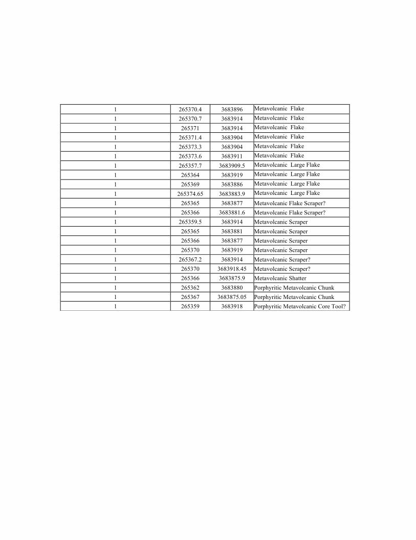
1 265370.4 3683896 Metavolcanic Flake

1 265370.7 3683914 Metavolcanic Flake

1 265371 3683914 Metavolcanic Flake

1 265371.4 3683904 Metavolcanic Flake

1 265373.3 3683904 Metavolcanic Flake

1 265373.6 3683911 Metavolcanic Flake

1 265357.7 3683909.5 Metavolcanic Large Flake

1 265364 3683919 Metavolcanic Large Flake

1 265369 3683886 Metavolcanic Large Flake

1 265374.65 3683883.9 Metavolcanic Large Flake

1 265365 3683877 Metavolcanic Flake Scraper? 1 265366 3683881.6 Metavolcanic Flake Scraper? 1 265359.5 3683914 Metavolcanic Scraper 1 265365 3683881 Metavolcanic Scraper 1 265366 3683877 Metavolcanic Scraper 1 265370 3683919 Metavolcanic Scraper 1 265367.2 3683914 Metavolcanic Scraper? 1 265370 3683918.45 Metavolcanic Scraper? 1 265366 3683875.9 Metavolcanic Shatter 1 265362 3683880 Porphyritic Metavolcanic Chunk 1 265367 3683875.05 Porphyritic Metavolcanic Chunk 1 265359 3683918 Porphyritic Metavolcanic Core Tool?

CA-SNI-25 Outdoor Activity Area CA-SNI-25 House Activity Area

Material Type Length (cm) metavolcanic flake 1.6 metavolcanic flake 1.8 metavolcanic flake 2.6 metavolcanic flake 2.6 metavolcanic flake 2.7 metavolcanic flake 2.9 metavolcanic flake 3.1 metavolcanic flake 3.3 metavolcanic flake 3.3 metavolcanic flake 3.3 metavolcanic flake 3.3 metavolcanic flake 3.5 metavolcanic flake 3.6 metavolcanic flake 3.6 metavolcanic flake 3.7 metavolcanic flake 3.9 metavolcanic flake 3.9 metavolcanic flake 4.4 metavolcanic flake 4.4 metavolcanic flake 5 metavolcanic flake 5 metavolcanic flake 5.1 metavolcanic flake 5.2 metavolcanic flake 5.5 metavolcanic flake 5.8 metavolcanic flake 5.9 metavolcanic flake 7.4

quartzite flake 3 quartzite flake 3.5 quartzite flake 3.8

Material Type Length (cm)

chalcedony flake 3.3 metavolcanic flake 1.1 metavolcanic flake 1.4 metavolcanic flake 1.5 metavolcanic flake 1.6 metavolcanic flake 1.7 metavolcanic flake 2.2 metavolcanic flake 2.2 metavolcanic flake 2.3 metavolcanic flake 2.4 metavolcanic flake 2.4 metavolcanic flake 2.5 metavolcanic flake 2.6 metavolcanic flake 2.9 metavolcanic flake 3.2 metavolcanic flake 3.4 metavolcanic flake 3.7 metavolcanic flake 3.8 metavolcanic flake 3.8 metavolcanic flake 5.1 metavolcanic flake 5.2 metavolcanic flake 5.3 metavolcanic flake 5.5 metavolcanic flake 5.6 metavolcanic flake 7

quartzite flake 3.1 quartzite flake 3.4 quartzite flake 3.4 quartzite flake 4.7 quartzite flake 6.1 quartzite flake 6.4

APPENDIX D: CA-SNI-11 TARRING PEBBLE DATA TABLE

CA-SNI-11 Tarring Pebbles Sample Mass (grams) Comments Location Unit Level 19-126 2.1 whole Mound B 1.5S/3E 10 to 20 cm 19-126 3.5 whole Mound B 1.5S/3E 10 to 20 cm 19-126 4 whole Mound B 1.5S/3E 10 to 20 cm 19-126 4 whole Mound B 1.5S/3E 10 to 20 cm 19-126 5.3 whole Mound B 1.5S/3E 10 to 20 cm 19-126 9.3 whole Mound B 1.5S/3E 10 to 20 cm 19-126 12 whole Mound B 1.5S/3E 10 to 20 cm 19-126 13.4 whole Mound B 1.5S/3E 10 to 20 cm 19-126 15.5 whole Mound B 1.5S/3E 10 to 20 cm 19-140 1.3 whole Mound B 1.5S/3E 10 to 20 cm 19-140 2.1 whole Mound B 1.5S/3E 10 to 20 cm 19-140 2.5 whole Mound B 1.5S/3E 10 to 20 cm 19-140 3 whole Mound B 1.5S/3E 10 to 20 cm 19-140 3.3 whole Mound B 1.5S/3E 10 to 20 cm 19-140 5.3 whole Mound B 1.5S/3E 10 to 20 cm 19-140 6.9 whole Mound B 1.5S/3E 10 to 20 cm 19-140 8.4 whole Mound B 1.5S/3E 10 to 20 cm 19-140 10.1 whole Mound B 1.5S/3E 10 to 20 cm 19-140 10.9 whole Mound B 1.5S/3E 10 to 20 cm 19-153 2.9 whole Mound B 1.5S/3E 20 to 30 cm 19-153 4.1 whole Mound B 1.5S/3E 20 to 30 cm 19-153 4.7 whole Mound B 1.5S/3E 20 to 30 cm 19-153 8.7 whole Mound B 1.5S/3E 20 to 30 cm 19-153 12.4 whole Mound B 1.5S/3E 20 to 30 cm 19-397 2.7 whole Mound B 3S/3E 0 to 30 cm 19-397 4.3 whole Mound B 3S/3E 0 to 30 cm 19-397 8.5 whole Mound B 3S/3E 0 to 30 cm 19-397 29.2 whole Mound B 3S/3E 0 to 30 cm 19-505 20 whole Mound B 1.5S/58.5W 30-40 cm 19-505 20.5 whole Mound B 1.5S/58.5W 30-40 cm 19-505 22.2 whole Mound B 1.5S/58.5W 30-40 cm 19-505 23.6 whole Mound B 1.5S/58.5W 30-40 cm 19-505 31.3 whole Mound B 1.5S/58.5W 30-40 cm 19-505 47.8 whole Mound B 1.5S/58.5W 30-40 cm

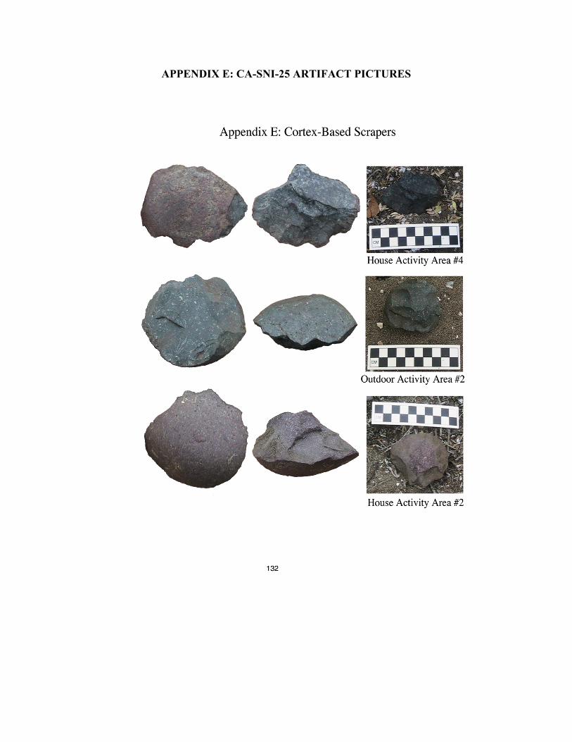
APPENDIX E: CA-SNI-25 ARTIFACT PICTURES