Banque de France Working Paper #633 June 2017

Accounting for Wealth Inequality Dynamics: Methods, Estimates and Simulations for

France (1800-2014)

Bertrand Garbinti1, Jonathan Goupille-Lebret2 & Thomas Piketty3

June 2017, WP #633

ABSTRACT

This paper combines different sources and methods (income tax data, inheritance registers, national accounts, wealth surveys) in order to deliver consistent, unified wealth distribution series for France over the 1800-2014 period. We find a large decline of the top 10% wealth share from the 1910s to the 1980s, mostly to the benefit of the middle 40% of the distribution. Since the 1980s-90s, we observe a moderate rise of wealth concentration, with large fluctuations due to asset price movements. In effect, rising inequality in saving rates and rates of return pushes toward rising wealth concentration, in spite of the contradictory effect of housing prices. We develop a simple simulation model highlighting how the combination of unequal saving rates, rates of return and labor earnings leads to large multiplicative effects and high steady-state wealth concentration. Small changes in the key parameters appear to matter a lot for long-run inequality. We discuss the conditions under which rising concentration is likely to continue in the coming decades.4

Keywords: saving rate, steady-state, wealth inequality

JEL classification: D31 E21 N34

1 Banque de France, CREST-Insee, bertrand.garbinti@banque-france.fr 2 Paris School of Economics, GATE-LSE, jonathan.goupille@ens.fr 3 Paris School of Economics, piketty@ens.fr 4 We are grateful to Facundo Alvaredo, Emmanuel Saez, Daniel Waldenström and Gabriel Zucman for numerous conversations. We are also thankful to Vincent Biausque for fruitful discussions about national accounts and to the DGFiP-GF3C team for its efficient help with fiscal data use and access. The research leading to these results has received funding from the European Research Council under the European Union's Seventh Framework Programme, ERC Grant Agreement n. 340831. This work is also supported by a public grant overseen by the French National Research Agency (ANR) as part of the « Investissements d’avenir » program (reference ANR-10-EQPX-17 – Centre d’accès sécurisé aux données – CASD). Updated files and series are available on the WID.world website (World Wealth and Income Database). The opinions expressed here are not necessarily those of the Banque de France or the Eurosystem.

Working Papers reflect the opinions of the authors and do not necessarily express the views of the Banque de France. This document is available on publications.banque-france.fr/en

Banque de France Working Paper #633 ii

NON-TECHNICAL SUMMARY

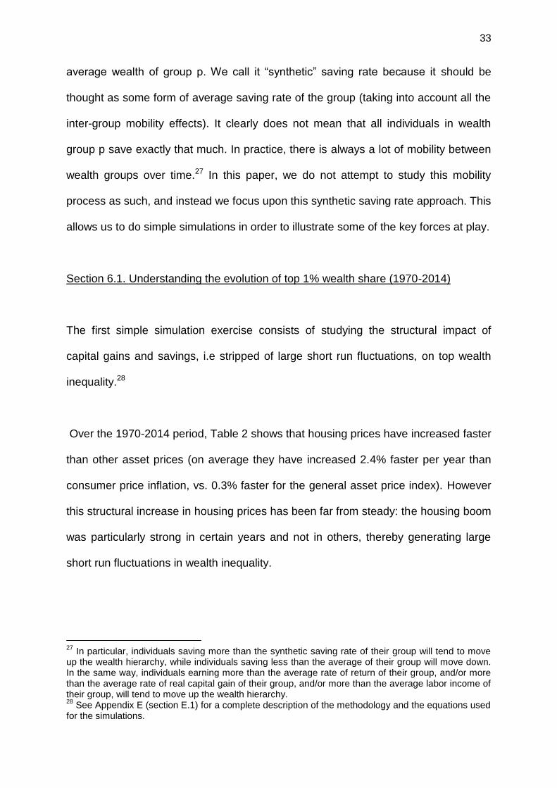
In France, the strong decrease in wealth inequality starts at the beginning of the 20th century. The share of total wealth held by the richest 10% decreases from more than 80% at the beginning of WW1 to 50% in the mid-80s. Meanwhile, we observe the “middle class” (middle 40%) rises and its wealth share ranges from 15% in 1914 to 40%. First, the rise of the middle 40% share during the 1914-1945 period is not due to the fact that the middle class accumulated a lot during this period. It simply corresponds to the fact the richest 10% were relatively more stricken by wealth shocks during this period (in proportion of their initial wealth). In contrast, during the post-war decade, the rise of the middle class corresponds to a significant rise of their absolute wealth level. A slight and continuous increase in inequality and with large fluctuations around 2000 due to financial asset price movements, since the portfolios of the top wealth shares are mainly composed them. The rise of housing prices observed in the 2000s has an ambiguous effect. It leads to a decrease in inequality between the middle class (whose portfolios are mainly composed of home owner housing) and an increase in inequality between the middle class and the poorest individuals (bottom 50%), and makes it more difficult the access to homeownership. Inequality in labor earnings, rates of return and synthetic saving rates are key-determinants to understand wealth concentration. We use the strong differences in these parameters observed between 1970-1984 and the 1984-2014 periods to show how small changes in these determinants are associated with strong differences in wealth concentration dynamics.

Banque de France Working Paper #633 iii

Dynamique de la concentration du patrimoine : Méthodes, estimations and simulations pour la France

(1800-2014) RÉSUMÉ

Ce papier associe plusieurs sources et méthodes (données fiscales, données successorales, comptabilité nationale, enquêtes ménages) afin de produire des séries cohérentes et unifiées de distribution du patrimoine par percentiles en France pour la période 1800-2014, détaillées par âge, sexe, type de revenus et d’actifs pour la période 1970-2014. Nous trouvons un large déclin de la part du patrimoine détenue par les 10 % les plus fortunés entre 1920 et le milieu des années 80 (de 80-90 % de la richesse totale au cours du 19è siècle et jusqu’à la première guerre mondiale, jusqu’à 50-60 % dans les années 1980), principalement au bénéfice des 40 % d’individus situés entre les 50 % les plus pauvres (dont la part de richesse reste inférieure à 10 %) et les 10 % les plus riches.

Depuis les années 1980, nous observons une hausse modérée de la concentration du patrimoine, avec de larges fluctuations dues aux mouvements des prix des actifs. La hausse des inégalités des taux d’épargne et des taux de rendement entrainent une hausse de la concentration malgré l’effet contradictoire des prix de l’immobilier. Nous développons un modèle simple qui souligne comment la combinaison des inégalités de taux d’épargne, de taux de rendement et de revenus du travail conduit à de larges effets multiplicatifs et une concentration élevée du patrimoine à l’équilibre stationnaire. De faibles variations dans ces paramètres-clés s’avèrent avoir un fort effet sur les inégalités à long terme. Nous discutons les conditions pouvant conduire à une hausse de la concentration au cours des prochaines décennies.

Mots-clés : épargne, équilibre stationnaire, inégalités de patrimoine Les Documents de travail reflètent les idées personnelles de leurs auteurs

et n'expriment pas nécessairement la position de la Banque de France. Ce document est disponible sur publications.banque-france.fr

1

Section 1. Introduction

Section 2. Relation to existing literature

Section 3. Concepts, data sources and methodology

Section 4. Long run wealth inequality series, 1800-2014

Section 5. Inequality breakdowns by age and assets, 1970-2014

Section 6. Accounting for wealth inequality: models and simulations

Section 7. International comparisons

Section 8. Concluding comments and research perspectives

References

2

Section 1. Introduction

Measuring the distribution of wealth involves a large number of imperfect and

sometimes contradictory data sources and methodologies. In turn, the lack of reliable

data series has made it very difficult for economists so far to test quantitative models

of wealth accumulation and distribution. In this paper, we attempt to show that these

measurement limitations can to some extent be overcome (using the case of France

as an illustration), and that the new resulting series can be used to better understand

the long-run determinants of wealth concentration.

This paper has two main objectives. Our first objective is related to the measurement

of wealth inequality. We show that various sources of wealth data and methods can

and should be reconciled and used together in order to obtain a consistent picture of

wealth inequality trends. We illustrate this general point using detailed data for the

case of France (a particularly interesting case, especially because of the early

availability of homogenous inheritance registers from 1800 onwards). In effect, we

combine different sources and methods (particularly income tax data, inheritance

registers, national accounts, wealth surveys) in order to deliver consistent, unified

wealth distribution series by percentiles for France over the 1800-2014 period.

Regarding the 1970-2014 period, we favor a mixed capitalization method based on

income tax data and household surveys. The income capitalization method is in our

view the most appropriate method for assets which generate taxable income flows

and for certain parts of the distribution which are not well covered in surveys

(particularly the top). However, it needs to be supplemented with additional

3

information coming from other data sources (particularly wealth surveys) regarding

certain tax-exempt assets and certain parts of the distribution (particularly the

bottom). Our mixed capitalization method allows us to highlight new dimensions of

wealth inequality. First, it offers detailed wealth inequality series broken down by

percentile, age, gender and asset categories for the 1970-2014 sub-period. Second,

it allows to estimate the joint distribution of income and wealth as well as the

determinants of wealth inequality dynamics such as rates of return, saving rates and

rates of capital gains by wealth groups.

Over the longer run, we link up our 1970-2014 series together with historical 1800-

1970 series that we construct using the estate multiplier method based on inheritance

tax data (the only data source and method available over such a long period). We

show that the two methods deliver consistent estimates over the 1970-2014 period,

which is reassuring and gives us confidence in the fact that we can link up the two

series. As a result, our unified series offer homogenous wealth inequality series

broken down by percentile covering the entire 1800-2014 period. We also offer

detailed comparisons and reconciliations with other data sources (wealth tax data

and billionaire lists) for the recent period, although we do not formally use them for

our benchmark series.

Our second objective is to use these new series in order to better understand the

long-run determinants of wealth concentration. The two general facts that emerge

from our series are, first, that wealth concentration is systematically much larger than

income concentration, and next, that the exact level of wealth concentration displays

strong variations over time. In particular, we confirm previous findings regarding a

4

significant decline in the top 10% wealth share between 1914 and 1984 (from 80-

90% of total wealth during the 19th century up until World War 1, down to 50-60% in

the early 1980s), mostly to the benefit of the middle 40% of the distribution (the

bottom 50% wealth share is always less than 10%). Since the mid-1980s, we

observe a moderate rise of wealth concentration, with large fluctuations due to asset

price movements. We also find wealth inequality is almost as large within each age

group as for the population taken as a whole.

Regarding the long-run fall of wealth inequality between 1914 and 1984, the most

natural interpretation is that top wealth groups were hit by a number of very large

capital shocks that occurred during the 1914-1945 period (destruction, depression,

inflation, nationalization, etc.). However, it is still a key challenge to understand how

the structural policy changes that occurred after these shocks (e.g. rise of

progressive taxation, social spending, financial regulation, rent control, etc.) have

permanently reduced the steady-state level of wealth inequality. While we cannot

evaluate the precise quantitative role played by each policy, we are able to better

explore the reasons for wealth inequality dynamics.

We develop a simple steady-state formula to better understand the observed

evolutions of wealth concentration. This formula highlights three key forces behind

long term wealth inequality dynamics: unequal labor incomes, unequal rates of return

and unequal saving rates. We show that the observed values of these parameters

during the 1970-1984 period are consistent with the observed long-run reduction in

wealth concentration over the 1914-1984 period. Regarding the post-1984 rise in

wealth concentration, we find that this reversal of the trend can be accounted for by

5

rising inequality in saving rates and rates of return (which could itself be due to a

mixture of factors, including growth slowdown, rising unemployment and labor

earnings inequality, and financial deregulation). This effect tends to dominate the

contradictory impact of rising housing prices (which in any case cannot continue in

the very long run). We present various simulations for the coming decades and

discuss the conditions under which rising wealth concentration is likely to continue,

and whether this trend can go all the way toward pre-WW1 inequality levels.

Our general conclusion is not that we can make predictions about the future evolution

of wealth concentration, but rather that relatively small changes in the key

parameters appear to matter a lot for long-run steady-state inequality of wealth. We

argue that in order to account for the high level of wealth concentration, one needs to

use a class of models combining unequal saving rates, rates of return and labor

earnings, as well as large dynamic multiplicative effects over long horizons.

We should also emphasize that the present paper is part of a broader multi-country

project in which we attempt to construct “distributional national accounts” (DINA), i.e.

detailed annual estimates of the distribution of income and wealth based on the

reconciliation between different fiscal sources, household surveys and

macroeconomic national accounts. The present paper focuses upon the wealth part

of the DINA series for France. In our companion paper (Garbinti, Goupille-Lebret and

Piketty, 2017), we combine tax, survey, and national accounts data in a

comprehensive and consistent manner to build new series on the distribution of

income in France over the 1900-2014 period.

6

In particular, the present work is closely related to recent work undertaken on the

long-run evolution of wealth and income distribution in the United States (Saez and

Zucman 2016; Piketty, Saez and Zucman 2016). More generally, the objective of the

multi-country project is to release data series that can be used by future research to

further investigate inequality dynamics and test formal models. All updated series will

be made available on the “World Wealth and Income Database” (WID.world) website

(http://WID.world). In our view, this provides an additional justification for the need to

develop more transparency and better administrative data on wealth.

The paper is organized as follows. Section 2 relates our work to the existing

literature. Section 3 presents our data sources and methodology. We then present

our main results, starting in section 4 with the long-run picture (1800-2014), and then

moving on in section 5 to the more detailed series available over the 1970-2014

period. In section 6 we discuss the possible interpretation behind our findings and

present our simulation results. In section 7 we compare our findings with recent

series constructed for other countries, and particularly with the U.S. series

constructed by Saez and Zucman (2016). Finally, section 8 offers concluding

comments. This paper is supplemented by an Online Data Appendix including

complete series and additional information about data sources and methodology.

7

Section 2. Relation to existing literature

Section 2.1. Literature on the historical evolution of wealth inequality

Our work builds upon a long tradition of research on wealth inequality measurement

dating back to the 19th century. It is also part of a recent project attempting to develop

consistent estimates of the distribution of income and wealth at the global level: the

“World Wealth and Income Database” (WID.world).

Economists and statisticians started using inheritance data in order to study the

wealth of the living in a systematic manner in the late 19th and early 20th centuries. A

large number of authors, often from the United Kingdom and France, independently

developed the “estate multiplier” method, first to estimate aggregate wealth of the

living from the aggregate inheritance flow, and subsequently in order to study wealth

distribution among the living by reweighting individual inheritance data (using the

inverse mortality rate of their age and gender group).1

It is only in recent decades, however, that these methods were used to construct

homogenous historical series on top wealth shares. Even today, such series are

available only for a handful of countries (in particular the U.S., the U.K., France,

Sweden and Australia). The first attempt to construct long-run top wealth shares

series using the estate multiplier approach was due to Lampman (1962), who

exploited U.S. estate tabulations over the 1922-1956 period. Atkinson and Harrison

(1978) then applied the estate multiplier method to British inheritance data over the

1 Some of the main references in this literature include Giffen (1878, 1889), Foville (1893), Colson

(1903), Levasseur (1907), Mallet (1908), Séaillès (1910), Strutt (1910), Mallet and Strutt (1915) and Stramp (1919). See Piketty (2011, p.1081-1083).

8

1923-1972 period. In addition, Atkinson and Harrison compared their estate-multiplier

top wealth shares series with alternative series based upon the income-capitalization

method (using income tax data) and showed that they are consistent.

In the case of France, top wealth shares covering the 1807-1994 period were first

constructed by Piketty, Postel-Vinay and Rosenthal (2006, 2014), using national

inheritance tabulations together with large micro-samples of inheritance declarations

collected in the Paris archives and other local archives.2 As compared to the U.S.

and the U.K, where homogenous estate data is not available until the early 20th

century, one key advantage of the French data is that it is available since 1800 (the

modern inheritance tax system was put in place in 1791 during the French Revolution

and hardly changed since then).

Long-run top wealth shares have also been constructed for Sweden by Roine and

Waldenström (2009) using both inheritance registers since the early 19th century and

annual wealth tax data since the early 20th century (when Sweden introduced an

annual wealth tax).

The U.S. series first constructed by Lampman (1962) were subsequently extended

until 2000 by Kopczuk and Saez (2004). More recently, Saez and Zucman (2016)

have argued that estate-multiplier series underestimate rising wealth concentration

for the latest decades, and that the rising inequality trend is better estimated by

income-capitalization series.

2 See also Bourdieu, Postel-Vinay and Suwa-Eisenmann (2003) and Bourdieu, Kesztenbaum and

Postel-Vinay (2013).

9

Our paper directly follows this literature. That is, we refine and update in various

ways the wealth inequality series constructed by Piketty, Postel-Vinay and Rosenthal

(2006, 2014). First, we estimate wealth series for all percentiles of the distribution,

from the bottom to the top, and not only for top groups, by relying on the complete

historical data from inheritance registers and inheritance tabulations and using

generalized, non-parametric Pareto interpolation techniques recently developed by

Blanchet, Fournier and Piketty (2017). Next, and most importantly, we link up our

historical inheritance-based wealth inequality series (covering the 1800-1970 period)

with new series that we construct for the 1970-2014 by using a mixture of income

capitalization and survey-based method. These new series allow us to highlight the

recent reversal of the decreasing trend that occurred since 1984. We also follow

Saez and Zucman (2016) in computing synthetic saving rate series by wealth groups,

which as we will show, offers a very powerful way to analyze the structural

determinants of wealth inequality and constitutes a useful complementary approach

to calibrated micro-founded theoretical models. Unlike Saez and Zucman (2016), we

are able to reconcile estate-multiplier and income-capitalization method for the recent

decades.

The reasons why we choose to favor the income-capitalization approach for our

1970-2014 series are twofold. First, this method offers joint annual information on

both wealth and income, which inheritance-based approaches cannot offer. Next, we

agree with Saez and Zucman (2016) that inheritance data and estate-multiplier

methods raise more and more problems in recent decades, especially because of

rising life expectancy (so that it is increasingly rare and abnormal to observe

decedent wealth at earlier ages) and intensive terminal tax planning (with extensive

10

private information about terminal illness). In addition, access to inheritance data has

deteriorated in a country like France (annual data is not available any longer, and

available data comes from samples with limited size). In case inheritance data was

annual and exhaustive, and income tax data was not, the situation would be different.

But given present data availability in France (and also in the U.S.), the most sensible

choice in our view is to use the income capitalization method. Of course the

conclusion could be different in other countries (such as the U.K.; see the recent

work by Alvaredo, Atkinson and Morelli, 2017).

Section 2.2. Literature on wealth distribution using household surveys

This paper is also closely related to recent research on wealth distribution using

household wealth surveys and Pareto adjustment for top wealth groups based upon

billionaire rankings.

Generally speaking, household wealth surveys have become very widespread in

recent decades.3 The development of wealth surveys has led to a new wave of

comparative wealth studies, with particular attention to the statistical modeling of the

distribution, from the very bottom - including segments with negative net wealth - to

the very top (see e.g. Cowell and Van Kerm (2015) for a survey article using HFCS

data for 15 Eurozone countries; see also Cowell (2013) for a comparison of wealth

distributions in the UK, Canada, Sweden and the U.S.).

3 One of the oldest and best established wealth surveys in the world is the SCF (Survey of Consumer

Finances) run by the U.S. Federal Reserve. The SCF has been conducted every three years since 1983 (the last survey was conducted in 2013; a preliminary SCF survey was conducted in 1962, but there was no other survey until 1983. see SCF, 2015). A number of European countries also started to conduct household wealth surveys during the 1980s-1990s. It is only in recent years, however, that there has been some serious attempt to homogenize European wealth surveys. The first wave of the HFCS (Household Finance and Consumption Survey) was conducted in 2010-11 in 15 Eurozone countries (see HFCS, 2015).

11

There has also been growing recognition in recent years that despite the best efforts

of the organizing institutions these wealth surveys suffer from major biases,

particularly regarding top wealth groups, and that new methods need to be

developed in order to correct for these biases in a systematic manner.4 The fact that

both the Federal Reserve and the ECB have limited ability to measure and monitor

the evolution of the distribution of wealth is increasingly regarded as highly

problematic, especially in light of the fact that quantitative-easing policies conducted

in recent years are likely to have major distributional consequences. In light of this,

several recent studies have attempted to reconcile administrative and wealth survey

data (Bricker et al. (2016)) or to use billionaire rankings and Pareto interpolation

techniques in order to correct upwards the top wealth levels reported in household

wealth surveys (see in particular Vermeulen (2016) and other references provided in

Blanchet, 2016).

Our contribution to this literature is twofold. First, we argue that wealth surveys and

Pareto adjustments using billionaire rankings can be useful, but that whenever

possible these sources and methods need to be used together with fiscal data (via

income capitalization, estate multiplier, and/or annual wealth tax methods). The

central advantages of fiscal sources are that - in addition to being available over

much longer time periods than wealth surveys and billionaire rankings – they are

annual (as opposed to wealth surveys, which are typically conducted every 3 to 5

years), they are exhaustive (i.e. they do not suffer from sampling problems: the entire

4 Although the SCF is usually regarded as the best existing wealth survey, recent research by Saez

and Zucman (2016) using fiscal data and the income capitalization method has shown that the SCF significantly underestimates rising wealth concentration in recent decades. The European HFCS is likely to suffer from even bigger biases, with potentially large variations between countries (since the methodologies used in each country are still far from being fully homogenous).

12

population is covered, rather than a small subsample), and they rely extensively on

third-party reporting and auditing (rather than self-reporting). These are key strengths

that cannot be neglected, especially given the many uncertainties surrounding self-

reporting biases in surveys, and the methodology used in billionaire rankings.

Next, in countries where fiscal sources do not exist and/or are not accessible, it is

critical to develop flexible, non-parametric generalized Pareto interpolation methods

(such as those developed by Blanchet, Fournier and Piketty, 2017) and to

systematically compare the patterns of Pareto coefficients with those obtained in

countries where fiscal data are available. There is still a long way to go before we can

use these methods in a reliable way.

Section 2.3. Literature on Calibrated Models of Wealth Distributions

Our work is also related to the large literature attempting to use dynamic quantitative

models of wealth inequality to replicate observed wealth inequality. As recently

surveyed by Piketty and Zucman (2015), Benhabib and Bisin (2016), De Nardi and

Fella (2017), several authors have recently introduced new ingredients into calibrated

micro-founded dynamics models, such as uninsured idiosyncratic shocks to labor

earnings and/or asset returns, tastes for savings and bequests, entrepreneurship,

preference heterogeneity.5 Typically, these models can generate substantial wealth

concentration at the top. For a given structure of individual-level shocks (unequal

labor incomes, saving rates, and rates of return), they also predict that the long-run

steady-state level of wealth inequality tends to be magnified if the gap r – g between

5 See among others Castaneda, Diaz-Gimenez and Rios-Rull (2003), De Nardi (2004), Cagetti and De

Nardi (2006), Aoki and Nirei (2016), Benhabib, Bisin, and Zhu (2015).

13

the net-of-tax rate of return r and the economy’s growth rate is larger (Piketty 2014,

chap.10; Piketty and Zucman 2015; Piketty 2015). However, while some ingredients

of these models taken separately or a combination of them help to reproduce the

level of wealth inequality at a point in time, more work is still needed to evaluate and

quantify rigorously the relative importance of each of these elements. Moreover,

these studies mostly abstract from the historical evolution of inequality and do not

explicitly simulate transitional dynamics.

Recently, three papers have investigated the ability of dynamic models to reproduce

and explain transition dynamics, from one stationary wealth distribution to another,

after a change in the economic environment. Gabaix, Lasry, Lions, and Moll (2016)

show that the baseline random growth model is not able to reproduce the observed

rise in the U.S top wealth shares since the early 1980s. To account for that fact, they

conjecture that one need to introduce either heterogeneity (type dependence) or

wealth-dependence (scale dependence) on both rates of returns and saving rates.6

Kaymak and Poschke (2015) show that the increase in U.S wealth inequality can be

explained by the historical changes in the tax and transfer system and by the

increase of wage inequality, which have affected differently the saving behaviors of

the bottom and middle income groups as compared to that of the top income group.

The crucial role of taxation in explaining the rise in U.S wealth inequality is also

emphasized by Hubmer, Krusell and Smith (2016). They find that the most important

driver is the significant drop in tax progressivity that started in the late 1970s.

6 The main purpose of Gabaix, Lasry, Lions, and Moll (2016) is to reproduce and explain the fast rise

in U.S top income inequality since the early 1980s. However, the online Appendix E of the paper is dedicated to the dynamics of wealth inequality.

14

These approaches using micro-founded calibrated models are of great interest, and

we see our work as complementary to these approaches.7 In particular, we provide

original series on the joint distribution of income and wealth along with labor income

share, rates of returns and synthetic saving rates by wealth groups that could be

useful to calibrate such models and to test their predictions. For instance, we show

that the rates of return and the saving rates are strongly positively correlated with

wealth. This evidence supports the claim of Gabaix, Lasry, Lions, and Moll (2016) to

introduce wealth-dependence (scale dependence) on both rates of returns and

saving rates in order to reproduce the rapid rise in wealth concentration observed

during the recent period. It would also be interesting to compare the saving rates

predicted by theoretical models (such as that of Hubmer, Krussel and Smith, 2016)

with observed synthetic saving rates. One of the limitations of the existing literature

on micro-founded dynamic wealth models is that they mostly attempt to reproduce a

given level – or change in levels – of wealth concentration, without testing explicitly

for the economic parameters and mechanisms – e.g. unequal saving rates, labor

incomes and rates of returns – generating such a pattern.

In the context of this particular paper, we do not go all the way toward a reconciliation

of the different approaches, in the sense that we calibrate a reduced-form dynamic

model using synthetic saving rates and rates of return per wealth fractiles, rather than

a fulll-fledged micro-found model. In effect, we do not model explicitly individual-level

shocks and mobility between wealth fractiles. The advantage is that we obtain very

simple and easy-to-calibrate steady-state formulas and simulations. But it is clear that

7 See also Fagereng, Guiso, Malacrino and Pistaferri (2016) and Bach, Calvet and Sodini (2016).

15

the next step is to embed these structural parameters into a micro model with

individual-level shocks.

We should also stress that France offers an interesting case to understand the

determinants of wealth inequality dynamics. Indeed, France has followed the same

pattern of wealth inequality as the U.S with decreasing inequality until early 1980s

and a reversal of this trend since then. But contrary to the U.S, there was no increase

in labor income inequality. To understand this pattern, we develop a very simple

steady-state formula that allows to study the impact of a change in key economic

parameters — growth rate, inequality in rates of returns, saving rates and labor

income — on both the stationary wealth distribution and the transition dynamics.

While our formula is much less sophisticated than the dynamic models, it relies on

stronger empirical basis. We show that the reversal of the trend in wealth inequality

since the early 1980s can be accounted for by rising inequality in saving rates in a

context of persistently high but stable inequality in rates of return. As a result, we

argue that in order to account for dramatic changes in wealth inequality dynamics,

one needs to use a class of models combining unequal saving rates, rates of return

and labor earnings, as well as large dynamic multiplicative effects over long horizons.

16

Section 3. Concepts, data sources and methodology

In this section we describe the concepts, data sources and main steps of the

methodology that we use in order to construct our wealth distribution series. Broadly

speaking, we combine three main types of data: national income and wealth

accounts; fiscal data (income tax returns and inheritance tax returns); and wealth

surveys. A longer and more complete discussion of the general methodological

issues involved in creating DINA estimates (not specific to France) is presented in

Alvaredo et al. (2016). Complete methodological details of our French specific data

sources and computations are presented in the Online Data Appendix along with a

wide set of tabulated series, data files and computer codes.

Section 3.1. Wealth and income concepts

Our wealth distribution series are constructed using a concept of "net personal

wealth" based upon national accounts categories.8 That is, net personal wealth is

defined as the sum of non-financial assets and financial assets, net of financial

liabilities (debt), held by the household sector. All these concepts are defined using

the latest international guidelines for national accounts (namely SNA 2008; for

additional details, see Alvaredo et al, 2016, and the Appendix). We break down non-

financial assets into housing assets and business assets. We include in housing

assets the value of the building and the value of the land underlying the building. We

include in business assets all non-financial assets held by households other than

housing assets. In practice, these are mostly the business assets held by self-

8 The reason for using national accounts concepts is not that we believe they are perfectly satisfactory.

Our rationale is simply that national accounts are the only existing attempt to define income and wealth in a consistent manner on an international basis.

17

employed individuals (but this also includes other small residual assets). We break

down financial assets into four categories: deposits (including currency and saving

accounts); bonds (including loans); equities (including investment funds shares); life

insurance (including pension funds). We therefore have seven asset categories

(housing assets, business assets, four financial asset categories, and debt), or

actually eight categories when we break down housing into owner-occupied and

tenant-occupied housing.

Also, our wealth distribution series always refer to the distribution of personal wealth

among individual adults (i.e. the net wealth of married couples is divided by two,

unless available information suggests to do differently).9

We use official national accounts established by INSEE for the recent decades (post-

1969 for national wealth accounts, and post-1949 for national income accounts). For

the earlier periods, we use the historical series provided by Piketty and Zucman

(2014). National income series for housing rental income (owner-occupied and

tenant-occupied), self-employment income, and interest and dividend income (which

are available separately for the four financial asset categories described above, at

least for the recent decades), allow us to compute average rates of return for

housing, business and financial assets, which we then use when we apply the

income capitalization method (see below).

9 With most methods, we do not observe adequate information that would allow us to split the wealth

of married couples on the basis of unequal individual property rights, so we revert to the equal-split method. With the estate multiplier method, however, we are sometimes able to directly observe own assets and community assets, so that we can compare equal-split wealth inequality estimates with unequal-split estimates.

18

Section 3.2. Mixed income capitalization-survey method (1970-2014)

We now describe the data sources and methodology used to estimate the distribution

of wealth for the 1970-2014 period. This is a mixed method, in the sense that it is

based both on the income capitalization method and on the survey-based method.

In order to apply the income capitalization method, we use the micro-files of income

tax returns that have been produced by the French Finance Ministry since 1970. We

have access to large annual micro-files since 1988. These files include about

400,000 tax units per year, with large oversampling at the top (they are exhaustive at

the very top; since 2010 we also have access to exhaustive micro-files, including

about the universe of all tax units, i.e. about 37 million tax units in 2010-2012).10

Before 1988, micro-files are available for a limited number of years (1970, 1975,

1979 and 1984) and are of smaller size (about 40,000 tax units per year).

We also have access to income tax tabulations, which have been produced by the

French Finance Ministry since the creation of income tax in France in 1914 (first

applied in 1915). These tabulations are available on an annual basis throughout the

1915-2014 period (with no exception) and are based upon the universe of all tax

units.11 They report the number of taxpayers and total income for a large number of

income brackets. By applying the generalized, non-parametric Pareto interpolation

techniques developed by Blanchet, Fournier and Piketty, 2017), they can be used to

estimate annual series on income percentiles (for all percentiles, from the bottom to

the top of the distribution of total income; see Garbinti, Goupille-Lebret and Piketty,

10

As of July 2016, the latest micro-file available is the 2012 micro-file. For years 2013-2014 we apply the same method as that described below for 1971-1974, 1976-1978, 1980-1983 and 1985-1987. 11

As of July 2016, the last tabulation available is the 2014 tabulation.

19

2017). These tabulations also include detailed breakdowns by income categories

(wages, self-employment income, dividend, interest, etc.), which we use to estimate

separately the distribution of labor income and capital income (see Garbinti, Goupille-

Lebret and Piketty (2017, Appendix D)). In principle, one could also use these

historical tabulations and the income capitalization method in order to estimate the

distribution of wealth prior to 1970. However these tabulations by income categories

suffer from a number of limitations, so that we prefer to use the income capitalization

method as our benchmark method solely for the 1970-2014 period (when we have

access to micro-files of income tax returns), and to adopt the estate multiplier method

(based upon inheritance tax returns) as our benchmark method prior to 1970.12

Thanks to the 1970-2014 income tax micro-files, we have access to detailed,

individual-level information on taxable asset income flows, including tenant-occupied

rental income, self-employment income, interest income, and dividend income.13 We

divide these flows by the relevant asset-specific average rates of return (as described

above) in order to compute the stock of tenant-occupied housing assets, business

assets, bonds, and equities.14

12

Generally speaking, the main limitation of income tax tabulations is that prior to 1985 they only cover tax units that are subject to positive income tax. Another specific limitation of tabulations by income categories is that prior to 1945 they only cover a limited number of years (namely, 1917, 1920, 1932, 1934, 1936 and 1937; they then become annual in 1945). In contrast, inheritance tax tabulations cover the entire distribution of wealth (whether the resulting asset income is subject to income tax), and they cover many more years prior to 1945. Full details on income tax tabulations and the way we exploit them are given in Garbinti, Goupille-Lebret and Piketty (2017, Appendix D). 13

Realized capital gains are reported in the tax returns. We exclude them from our analysis for two reasons. First, only realized capital gains, i.e. capital gains resulting from the sale of an asset, have to be reported in the income tax returns. Second, the capital gains reported correspond to the cumulative of all past capital gains (since the purchase of the asset) rather than those of the current period. 14

We interpolate the missing years 1971-1974, 1976-1978, 1980-1983 and 1985-1987 by using annual aggregate series by asset categories and by assuming linear trends in within-asset-class distribution. As an alternative strategy, we also used annual income tax tabulations (broken down by income categories) and found that this makes very little difference.

20

The next step is to deal with assets that do not generate taxable income flows,

namely owner-occupied housing, life insurance, and deposits (including currency and

saving accounts).15 We use available wealth surveys in order to impute these assets

on the basis of labor income, financial income and age. Housing surveys (including

information on housing assets and debt) were conducted by INSEE in 1970, 1973,

1978, 1984, 1988, 1992, 1996, 2002, 2006, 2010 and 2013. Household wealth

surveys (including housing, business and financial assets and debt) were conducted

by INSEE in 1986, 1992, 1998, 2004, 2010 and 2014.16 The 2010 and 2014 wealth

surveys are the French component of the Eurosystem HFCS survey and are more

sophisticated than previous surveys.17 We conducted sensitivity tests and applied

several alternative imputation methods for tax-exempt assets using housing and

wealth surveys over the 1970-2014 period, and the general conclusion is that the

overall impact on wealth distribution series is extremely small (Figures B7 to B12,

Appendix B).

By construction, our methodology delivers individual-level information on both wealth

and income over the 1970-2014 period (which we will later use to compute synthetic

saving rates and to perform simulations), together with detailed breakdowns by age,

gender, and asset categories.

All data files, computer codes and robustness checks regarding our mixed income

capitalization-wealth survey method are given in the Data Appendix (Appendix B).

15

Note that owner-occupied rental income (i.e. imputed rent) was included in taxable income in France from the creation of the income tax until 1963. 16

These wealth surveys were called « enquête actifs financiers » in 1986 and 1992, and « enquête patrimoine» since 1998. Housing surveys were always called « enquête logement ». 17

The 2010 and 2014 surveys include answers with exact amounts (rather than answers by wealth brackets, which were used in previous surveys) and large oversampling at the top (although the sample size of the survey is still insufficient to go beyond the 99

th percentile).

21

Section 3.3. Estate multiplier method (W2) (1800-1970)

We now describe the date sources and the estate multiplier methodology that we use

in order to estimate the distribution of wealth over the 1800-1970 period.

The main reason for using the estate multiplier technique over the 1800-1970 period

is simply that this is the only data source and method available over such a long time

period. The income tax was created in France in 1914, so there is no data on capital

income flows prior to this date. In contrast, the modern inheritance tax was set up in

1791, and individual-level inheritance registers have been well preserved and are

accessible to researchers since 1800. These registers include detailed information

about assets, age, and gender, in principle for all decedents (irrespective of the level

of their wealth), so they constitute the ideal source to apply estate multiplier

techniques. That is, we reweight the distribution of wealth at death by using the

mortality rate of the relevant age-gender cell (with standard corrections for differential

mortality), so as to recover the distribution of wealth among the living. Regarding the

1800-1902 period, we refine the estate-multiplier estimates already computed by

Piketty, Postel-Vinay and Rosenthal (2006, 2014) on the basis of the large individual-

level micro-samples of estates which they collected in Paris inheritance registers and

of the provincial samples collected by Bourdieu et al (2003, 2013) in the context of

the TRA survey.

In 1902 the French inheritance tax was made progressive, and the tax administration

started to compile detailed tabulations reporting the number of decedents and

22

amount of their wealth for a large number of inheritance brackets. These tabulations

are consistent with the data collected in inheritance registers, and they are available

on a quasi-annual, exhaustive national basis between 1902 and 1964 (except for the

1914-1924 sub-period). They occasionally include supplementary breakdowns by

age brackets and asset categories. We use these national tabulations (together with

the estate multiplier method and the Pareto interpolation techniques developed by

Blanchet, Fournier and Piketty, 2017) in order to compute our wealth distribution

series for the 1902-1970 period.18

Unfortunately, annual inheritance tabulations were interrupted by the French Finance

Ministry in 1964. Instead, for the recent decades, the tax administration compiled

national micro-samples of inheritance tax returns in 1977, 1984, 1987, 1994, 2000,

2006 and 2010 (with limited sample size). We applied the estate multiplier method to

the 1984-2010 samples (the 1977 file is not usable), together with correction for tax-

exempt assets (particularly life insurance), and we refine previous estimates using

differential mortality rates.19 We found that the resulting estate multiplier method

estimates for the wealth distribution are extremely close to the estimates coming from

our mixed income capitalization-survey method. This is reinsuring and gives us

confidence that we can link up our 1800-1970 estate-multiplier series with our 1970-

2014 income-capitalization-survey series (Figures D1 to D4, Appendix D).20

18

We complete the missing years 1914-1924 and 1965-1969 by using data on top capital incomes from income tax tabulations. 19

We detail how to take into account differential mortality rates for different wealth groups and present a general formula in Appendix D. 20

In principle, one could return to individual-level inheritance registers to collect annual samples for the recent decades; unfortunately it is very difficult to access these registers for the recent period.

23

All data files, computer codes and robustness checks regarding the estate multiplier

method are given in the Data Appendix (see Appendix C for estate-multiplier

estimates over the 1800-1970 period, and Appendix D for reconciliation between

estate-multiplier and income-capitalization estimates for the 1984-2010 period).

Section 3.4. Reconciliation with other methods

We also provide in the Data Appendix detailed computations in order to reconcile our

benchmark series with other available methods for the recent period (see Appendix F

for reconciliation with wealth surveys, Appendix G for reconciliation with wealth tax

data, and Appendix H for reconciliation with billionaire lists).

As we mentioned above, the latest wealth surveys (2010 and 2014) are of relatively

high quality and are matched with income tax declarations. The main limitation is

their sample size, which is too small to go beyond the 99th percentile. In effect, very

top capital income and wealth levels are under-estimated in wealth surveys. To take

into account misreporting and non-response at the top, we assume differential

reporting rates (estimated thanks to comparison with National Accounts).21 We show

that using differential reporting rates just for equities and bonds allows to obtain top

wealth shares series that are consistent both in trend and level with those from our

benchmark method (Figures F1 and F2, Appendix F).

We also compare the top wealth levels estimated in our benchmark series with the

top wealth levels that can be estimated using wealth tax tabulations that are available

21

The different steps of our estimation are fully described in our Appendix, section F.2.

24

over the 1982-2013 period (with a number of missing years). A progressive annual

tax on top wealth holders (approximately the top 1%) was instituted in France in 1982

(IGF), abolished in 1986, re-instituted in 1989 (ISF), and still in place in 2016. There

has been very limited access to micro-files so far, but tabulations by wealth brackets

have been published on an irregular basis since 1982. The main difficulty with this

data is that there are many tax-exempt assets, in particular regarding equity

participations in family firms and in companies where asset holders play an active

management role (the exemption for so-called “professional assets”). By making

plausible assumptions on the fraction of tax-exempt wealth by asset categories and

levels, we are able to reconcile this data with our benchmark estimates. Figures G2

to G5 (Appendix G) show consistent patterns and levels between our adjusted wealth

tax series and our benchmark wealth inequality series. But there is significant

uncertainty about the exact level and evolution of tax exemptions, so it is difficult to

use this source on its own.

Finally, we also compare our benchmark estimates with the top wealth levels that can

be estimated using the billionaire list published by magazines (Challenges at the

French level and Forbes at the global level). The main difficulty here is that very little

is known about how these lists are established, and also about the size of the family

unit. By making plausible assumptions on the distribution of family unit size, we are

able to reconcile this data with our benchmark estimates (Figure H2, Appendix H).

However we conclude that there is so much uncertainty about billionaire lists that

they should be used with a lot of caution (in addition to other sources rather than on

their own).

25

Section 4. Long-run wealth inequality series (1800-2014)

We now present our benchmark unified series for wealth distribution in France over

the 1800-2014 period.

The wealth levels, thresholds and shares for 2014 are reported on Table 1. In 2014,

average net wealth per adult in France was about 200,000 €. Average wealth within

the bottom 50% of the distribution was slightly more than 20,000 €, i.e. about 10% of

the overall average, so that their wealth share was close to 5%. Average wealth

within the next 40% of the distribution was slightly less than 200,000 €, so that their

wealth share was close to 40%. Finally, average wealth within the top 10% was about

1.1 million € (i.e. about 5.5 times average wealth), so that their wealth share was

about 55%.

We report in Figure 1 the evolution of the wealth shares going to these three groups

over the 1800-2014 period. The wealth share going to the bottom 50% (the “lower

class”) has always been very small (less than 10%). The major long-run

transformation is the rise of the share going to the middle 40% (the “middle class”)

and the decline of the share going to the top 10% (the “upper class”). This major

change entirely took place between 1914 and the early 1980s.

During the 19th and early 20th century, up until World War 1, the top 10% share is

relatively stable at very high levels – between 80% and 90% of total wealth, with a

slight upward trend over the period. The middle 40% share was relatively small

throughout the period, e.g. slightly above 10% at the eve of World War 1, not very

26

much above the bottom 50% share. In a sense there was no “middle class”: the

middle 40% was almost as property-less as the bottom 50%.

The top 10% wealth share started to fall following the 1914-1945 capital shocks, and

the fall continued until the early 1980s, with an absolute minimum in 1983-1984 (with

slightly more than 50% of total wealth). Here it is interesting to recall that the

aggregate wealth-national income ratio fell hugely over the 1914-1945 period - from

about 700% to less than 200% - and gradually recovered in the decades following

World War II.22 In this work, we are able to study the distributional trends of the

wealth-income ratios. We show that the rise of the middle 40% share during the

1914-1945 period is not due to the fact that the middle class accumulated a lot of

wealth during this period: this simply corresponds to the fact they lost less wealth – in

proportion to their initial wealth level – than the top 10%. In contrast, during the post-

war decades, the rise of the middle class corresponds to a significant rise of their

absolute wealth levels (see Figures FA6 to FA8, Appendix A for detailed series).

In the recent decades, we observe a moderate rise in the top 10% wealth share, and

a corresponding erosion of the middle 40% wealth share. However we also notice

strong short-run fluctuations, with a large rise in top 10% share up to 2000, followed

by a sharp decline. As we will see below, this is entirely due to large movements in

relative asset prices (stock prices are very high as compared to housing prices in

2000, which favors the upper class relative to the middle class).

22

See Piketty and Zucman (2014) for a detailed analysis and decomposition of the aggregate wealth-income ratio between the various explanatory factors: destructions, inflation, lack of investment, and a general fall in asset price indexes as compared to consumer price indexes, partly due to rent control and other regulations.

27

Next, it is worth stressing that the historical decline in the top 10% wealth share is

entirely due to the collapse in the top 1% wealth share, from 55%-60% of total wealth

on the eve of World War 1 to 30% in 1945 and 15% in the early 1980s, back up to

about 25% in the early 2010s (see Figure 2).

Finally, we compare on Figures 3-4 our wealth inequality series with the income

inequality series coming from our companion paper (Garbinti, Goupille-Lebret and

Piketty, 2017). The central finding is that wealth concentration is always a lot larger

than labor income concentration and much more volatile. For instance, the share of

total labor income going to top 10% labor income earners always fluctuates around

25%-30% over the 1900-2014 period, while the share of total wealth going to top

10% wealth holders fluctuates in the 50%-90% range (see Figure 3). The comparison

is even more striking for the top 1% share: it fluctuates in the 5%-8% range for labor

income, and in the 15%-60% range for wealth (see Figure 4). The concentration of

total income (including labor and capital income) is intermediate between the two,

and closer to the concentration of labor income (which is not too surprising, given that

the labor share is typically around 65%-75% of total income).

It is striking to see that the long-run decline in income inequality is entirely due to the

decline in the concentration of wealth and capital income. This makes it even more

important to understand the long-run determinants of wealth concentration. Note also

that the concentration of capital income is even larger than the concentration of

wealth, which corresponds to the fact that higher wealth individuals tend to own

assets with higher rates of return - typically equity rather than housing or deposits

(more on this below).

28

Section 5. Wealth inequality breakdowns by age and assets, 1970-2014

We now present our detailed wealth inequality breakdowns by age and asset

categories for the 1970-2014 period. We begin with age decomposition and then

proceed with asset decompositions.

If we first look at the age-wealth profile, we find that average wealth is always very

small at age 20 (less than 15% of average adult wealth), then rises sharply with age

until age 50-55, and finally stabilizes or slightly declines at very high levels (around

120%-150% of average adult wealth) at ages 60-85. This age-wealth profile appears

to be relatively stable over the 1970-2014 period (see Figure 5).23 The key difference

with the standard Modigliani triangle (implied by a pure life-cycle model with no

bequest) is that average wealth does not seem to decline at high ages: it remains

stable at very high levels, which means that old-age individuals die with substantial

wealth and transmit it to their offspring. Note also that old-age individuals make very

substantial inter vivos gifts in France, so that average wealth at high ages would be

even higher without these gifts, particularly at the end of the period. Gifts are made

on average about 10 years before death, and the aggregate gift flow has increased

from about 20%-30% of the aggregate bequest flow in the 1970s to as much as 80%

of the aggregate bequest flow in the 2000s-2010s (see Piketty, 2011).24

23

The complete series of age-wealth profiles over the 1970-2014 period are reported in Table B21 of Appendix B. 24

In other words, when we observe in Figure 5 that the average wealth of 80-year-old individuals is about 140% of average adult wealth in 2010, it is important to keep in mind that this is the average wealth of individuals who have already given away almost half of their wealth (on average).

29

Next, it is interesting to see that wealth inequality is almost as large within each age

group than for the population taken as a whole (see Figure 6). For instance, if we

look at the distribution of wealth within the individuals aged 60-year-old and over, we

find a top 10% wealth share equal to 56% in 1970 (vs 59% for the population taken

as a whole) and to 49% in 2012 (vs 55% for the population taken as a while).

Before we move to inequality breakdowns by asset categories, it is important to recall

that the composition and level of aggregate wealth have changed substantially in

France over the 1970-2014 period (see Figures 7-8). Namely, the shares of housing

assets and financial assets have increased substantially, while the share of business

assets has declined markedly (due to the fall in self-employment). Financial assets

(other than deposits) increase strongly after the privatization of the late 1980s and

the 1990s and reach a high point in 2000 (stock market boom). In contrast, housing

prices decline in the early 1990s, and rise strongly during the 2000s, at the same

time as stock prices fall.

These contradictory movements in relative asset prices have an important impact on

the evolution of wealth inequality, because the difference wealth groups own very

different asset portfolios. As one can see in Figure 9, the bottom 30% of the

distribution own mostly deposits in 2012. Then housing assets become the main form

of wealth for the middle of the distribution. As we move toward the top 10% and the

top 1% of the distribution, financial assets (other than deposits) gradually become the

dominant form of wealth. This is particularly due to large equity portfolios. We find the

same general pattern throughout the 1970-2014 period, except that business assets

played a more important role at the beginning of the period, particularly among

30

middle-high-wealth holders (see Appendix B, Figures B20 to B23). If we now

decompose by asset categories the evolution of the wealth shares going to the

bottom 50%, middle 40%, top 10%, and top 1%, then we see very clearly the impact

of asset price movements on wealth shares, and particularly the impact of the 2000

stock market boom on the top 1% wealth share (see Figures 10-11 and Figures B24

to B28 from Appendix B). We return to this issue below.

31

Section 6. Accounting for wealth inequality: models and simulations

How can we account for our findings? Here it is important to distinguish short-run

evolutions (which can typically be driven by sharp movements in relative asset

prices) from long-run trends. From a long-run, structural perspective, how can we

account for the very high levels of wealth concentration that we observe in the data,

as well as the variations of these very high concentration levels across the 20th

century? First of all, it is clear that a life-cycle model with no bequest is not going to

generate sufficient inequality. Typically, in a standard life-cycle model, wealth

inequality within age group should be comparable in magnitude to the inequality of

labor income within age group, which is not at all what we observe. In addition, we

have seen from age-wealth profiles that decedents die with very substantial wealth. A

model with precautionary saving is not going to work very well either, since this

typically generates less wealth inequality than the cross-sectional inequality of labor

income shocks. In order to generate substantial wealth concentration and fat Pareto

upper tails for the wealth distribution, the most natural and flexible way to proceed is

to use dynamic wealth accumulation models with long horizon and with multiplicative

random shocks (see e.g. Aoki and Nirei (2016); Benhabib, Bisin and Zhu (2011,

2015); Piketty and Saez (2013); Piketty and Zucman (2015) and Hubmer, Krusell and

Smith (2016) for a survey). In this class of models, several structural forces tend to

amplify wealth inequality toward high steady-state levels, particularly the inequality of

saving rates and the inequality of rates of return, together with the inequality of labor

incomes.25

25

In the benchmark infinite-horizon, dynastic model with no random shock, any distribution of wealth (together with any exogenous distribution of labor income, and any exogenous correlation between the two) can be a steady-state. In effect, each dynasty saves a fraction g/r of its capital income so that all dynastic wealth levels grow at the same rate g (dynasties with no initial wealth save nothing, and

32

In order to illustrate this point and quantify these effects in a simple and transparent

manner, we will decompose our series using the following transition equation:

Wpt+1 = (1 + qp

t )[Wpt + sp

t (YpLt + rp

t Wpt )]

With: Wpt, W

pt+1 = average real wealth of group p at time t and t+1 (for instance, group

p could be the top 10% wealth group)

YpLt = average real labor income of group p at time t

rpt = average rate of return of group p at time t

qpt = average rate of real capital gains of group p at time t (real capital gains are

defined as the excess of average asset price inflation, given average portfolio

composition of group p, over consumer price inflation)26

spt = synthetic saving rate of group p at time t

We define synthetic saving rates in the same way as Saez and Zucman (2016). That

is, we can observe variables Wpt, W

pt+1,Y

pLt, r

pt, q

pt in our 1970-2014 series, and from

this we compute spt as the synthetic saving rate that can account for the evolution of

dynasties with a lot of initial wealth save enough to maintain their position, hence the full persistence result). The only equilibrium condition is the well-known modified-Golden-rule steady-state condition for aggregate rate of return (and therefore aggregate capital): r = θ + γg (where θ is the rate of time preference and γ the curvature of the utility function). The problem of this deterministic model is that it is too extreme (zero mobility, complete persistence of any initial wealth inequality). In effect the simple dynamic accounting model that we describe below is similar in spirit to the dynastic model, except that it allows for mobility and for any dispersion of saving rates (less extreme than in the dynastic model), as well as for any dispersion of rates of return. 26

For each wealth group, the rates of returns are computed by weighting each asset-specific rate of return – such as reported in the National Accounts – by the proportion of each asset in the wealth of the group. We follow the same methodology to compute the rates of capital gains by wealth group. Tables B5a to B9 from Appendix B report saving rates, rates of return and rates of capital gains by wealth group.

33

average wealth of group p. We call it “synthetic” saving rate because it should be

thought as some form of average saving rate of the group (taking into account all the

inter-group mobility effects). It clearly does not mean that all individuals in wealth

group p save exactly that much. In practice, there is always a lot of mobility between

wealth groups over time.27 In this paper, we do not attempt to study this mobility

process as such, and instead we focus upon this synthetic saving rate approach. This

allows us to do simple simulations in order to illustrate some of the key forces at play.

Section 6.1. Understanding the evolution of top 1% wealth share (1970-2014)

The first simple simulation exercise consists of studying the structural impact of

capital gains and savings, i.e stripped of large short run fluctuations, on top wealth

inequality.28

Over the 1970-2014 period, Table 2 shows that housing prices have increased faster

than other asset prices (on average they have increased 2.4% faster per year than

consumer price inflation, vs. 0.3% faster for the general asset price index). However

this structural increase in housing prices has been far from steady: the housing boom

was particularly strong in certain years and not in others, thereby generating large

short run fluctuations in wealth inequality.

27

In particular, individuals saving more than the synthetic saving rate of their group will tend to move up the wealth hierarchy, while individuals saving less than the average of their group will move down. In the same way, individuals earning more than the average rate of return of their group, and/or more than the average rate of real capital gain of their group, and/or more than the average labor income of their group, will tend to move up the wealth hierarchy. 28

See Appendix E (section E.1) for a complete description of the methodology and the equations used for the simulations.

34

Figure 12 reports the simulated top 1% wealth shares when we replace either the

time varying rates of real capital gains or both the time varying rates of real capital

gains and the time varying saving rates by their averages over the period 1970-

2014.29 By construction, all simulated series end up in 2014 at the same inequality

level as the observed series. The difference is that we now see a gradual increase in

inequality, rather than a sharp rise until 2000 followed by a decline. This confirms that

the only reason for this inverted-U-shaped pattern is due to variations in relative

asset prices, and more specifically to the stock market boom of 2000 (together with

the low housing prices of 2000). Once this is corrected by our simulated series, this

sharp decline disappears: in other words the structural parameters at play during this

period push toward rising concentration of wealth.30

We report in Figure 13 the simulated series that we obtain by replacing time varying

rates of capital gains and synthetic saving rates by their averages over the 1970-

2000 period, i.e. over the period ending before the housing boom of the 2000s. We

find that the top 1% share would have increased a lot more by 2012. In other words,

the housing boom of the 2000s has played an important role as a mitigating force to

limit the rise of inequality. More generally, the structural increase in top 10% and top

1% wealth shares over the 1984-2012 period would have been substantially larger

had housing prices not increased so fast relative to other asset prices. It should be

29

The constant capital gains are equal to the average structural changes of the various asset prices over the 1970-2014 period. 30

One potential concern with the capitalization method is that it can potentially overestimate the level of inequality during a stock boom in case the wealthiest individuals tend to benefit from higher returns (within a given asset class) than the rest of the population, and particularly so during booms (maybe because they pick more risky assets within a given asset class). In this case, top wealth shares and synthetic saving rates would tend to be upwardly biased, and particularly so during booms (see Bach et al (2016) on Swedish data). In the case of France, however, we show in the simulations that the huge hump-shape around 2000 is entirely due to short term price fluctuations (see Figure FE4, Appendix E). Moreover, our saving rates for the top 1 % are not increasing and turns out to be stable since the early 2000s (see table TB8, Appendix B).

35

noted however that rising housing prices have an ambiguous and contradictory

impact on inequality: on the one hand they raise the market value of the wealth of

middle class members who were able to access real estate property, thereby raising

the middle 40% wealth share relative to the top 10% wealth share; but on the other

hand rising housing prices make it more difficult for lower class members (or of

middle class members with no family wealth at all) to access real estate property.

Section 6.2. Simulating long-term wealth inequality

We now turn to very long term forces and simulations. Assume the relative capital

gain channel disappears, i.e. all asset prices rise at the same rate in the long run

(which must happen at some point, otherwise there will be only one asset left in the

long run), and this rate is the same as consumer price inflation (otherwise wealth-

income ratio would go to infinity).31 How is the long-run, steady-state level of wealth

concentration determined? By manipulating the transition equation given above for

wealth group p (for instance p = top 10% wealth group) and the corresponding

equation for aggregate wealth, one can easily derive the following steady-state

equation:

𝑠ℎ𝑤𝑝 = (1 +

𝑠𝑝 ∙ 𝑟𝑝 − 𝑠 ∙ 𝑟

𝑔 − 𝑠𝑝 ∙ 𝑟𝑝) ∙

𝑠𝑝

𝑠∙ 𝑠ℎ𝑌𝐿

𝑝

With: 𝑠ℎ𝑤𝑝

(resp. 𝑠ℎ𝑌𝐿𝑝

) is the share of wealth (resp. labor income) held by wealth

group p (for instance p = top 10% wealth group)

g is the economy’s growth rate

31

In Appendix E, we also extend our formula to include potential capital depreciation or appreciation

and show that the intuitions and mechanisms remain the same.

36

s the aggregate saving rate

r the aggregate rate of return

sp the synthetic saving rate of wealth group p

rp the rate of return of wealth group p (given their portfolio composition)

This formula can be derived very simply (see Appendix E) and is very intuitive.

For instance, if sp = s and rp = r (i.e. top wealth group has the same saving rate and

rate of return as average), then 𝑠ℎ𝑤𝑝 = 𝑠ℎ𝑌𝐿

𝑝, i.e. wealth inequality is exactly the same

as labor income inequality.

But if sp > s and/or rp > r (i.e. top wealth group saves more and/or has a higher rate of

return than average), then this can generate large multiplicative effects, and lead to

very high steady-state wealth concentration.32

The important point is the strength of these multiplicative effects. In order to illustrate

this, we have done the following simulations. First, we have computed the evolution

of synthetic saving rates for the different wealth groups over the 1970-2014 period.

The results are represented in Figure 14. As one can see, the high levels of wealth

concentration that we observe in France over this period can be accounted for by

highly stratified saving rates between wealth groups: while top 10% wealth holders

save on average between 20% and 30% of their annual income, middle 40% and

bottom 50% wealth groups save a much smaller fraction of their income.33 It is also

32

The difference with the steady-state formula presented by Saez and Zucman (2016) is that they relate wealth shares to total income shares (including both labor incomes and capital incomes, which themselves depend on wealth shares), so that they do not fully capture multiplicative effects between labor income inequality and steady-state wealth inequality. 33

Previous work on savings has mainly studied saving rates across income groups. They generally find that saving rate increases with current and permanent incomes (see for instance Dynan, Skynner,

37

striking to see that middle and bottom wealth groups use to save more in the 1970s

(with a saving rate of about 15% for the middle 40% and 8% for the bottom 50%)

than what we see since the 1980s-1990s (with a saving rate around 5% for the

middle 40% and close to 0% for the bottom 50%). This is the key structural force

which is accounting for rising wealth concentration in France over this period. This is

similar to what was found by Saez and Zucman (2016) for the U.S. case.

Next, we computed the evolution of flow rates of return (excluding capital gains,

which we assume to be zero in our simulations) for the different wealth groups over

the 1970-2014 period. The results are represented in Figure 15. As one can see,

higher wealth groups tend to have substantially higher rates of return. This large

inequality of rates of return is due to the large portfolio differences that we

documented earlier. In particular, top wealth groups own more financial assets like

equity with higher rates of return than housing or deposits (see Table 2).34

Finally, we use these estimates of sp and rp by wealth group in order to simulate

steady-state trajectories for the top wealth shares in coming decades. The main

Zeldes (2004) on US data, Bozio et al (2016) on UK data, Garbinti and Lamarche (2014a) on French data). Since wealth and income are strongly correlated, these conclusions are consistent with the gradient highlighted by our estimates. Another strand of the literature has studied the marginal propensity to consume out of wealth. For instance, Elinder, Erixson and Waldenström (2016) find evidence that the rich save new wealth (bequests) while the poor consume it. Garbinti and Lamarche (2014b, Table 2, http://www.insee.fr/fr/statistiques/1374588?sommaire=1374593) also show a large gradient in French saving rates across wealth groups, with the same order of magnitude as our synthetic saving rates (for instance, the median saving rate equals 30% for the top 20% of wealth distribution). 34

It is worth noting that on average real capital gains are relatively small (+0.3% per year) regarding personal wealth accumulation over the 1970-2014 period. In effect, the highly positive real capital gains recorded for housing assets (housing prices have increased faster than consumer price inflation) are almost entirely counterbalanced by the negative real capital gains for financial assets (particularly for deposits, bonds and other nominal assets, which by construction incur real capital losses equal to consumer price inflation). Note that average real capital gains are more substantial regarding national wealth accumulation (due to the fact that the real capital losses incurred by the personal sector on public bonds are the counterpart of the real capital gains made by the government sector). See Piketty and Zucman (2014) for detailed decompositions.

38

results are reported in Figure 16 for the top 10% wealth share. Additional top 10%

wealth share simulations based on alternative variants for saving rates and rates of

returns for the different wealth groups are reported in Appendix E.

For simplicity, we report only two simulations in Figure 16. First, we assume that the

same inequality of saving rates that we observe on average over the 1984-2014

period (namely 24.5% for the top 10% wealth group, and 2.5% for the bottom 90%)

will persist in the following decades, together with the same inequality of rates of

return and the same inequality of labor income.35 The conclusion is that the top 10%

wealth share will gradually increase in the future and will finally converge toward a

level of wealth inequality that is similar to that observed in the 19th and early 20th

centuries (namely about 80% of total wealth).

The other simulation consists of assuming the same inequality of saving rates that we

observe on average over the 1970-1984 period (namely 22% for the top 10% wealth

group, and 9.5% for the bottom 90%) would have persisted between 1984 and 2012

and during the following decades, together with the same inequality of rates of return

and the same inequality of labor income. The conclusion is that the top 10% wealth

share would have continued the declining path observed before 1984 and would

have gradually converged toward a substantially lower level of wealth concentration

(with a top 10% wealth share of about 45%).

There are two main messages from these simple simulations. First, relatively small

changes in the key parameters – inequality of saving rates and inequality of rates of

35

Note that the parameter shpYL reflects both the inequality of labor income and the correlation

between the distributions of wealth and labor income. For simplicity we assume both to be constant in future decades in our basic simulations. See appendix E for more details and other simulations.

39

return – can have enormous impact on steady-state wealth inequality. Next, these

effects take a very long time – many decades and generations – before they fully

materialize. This can explain why declining wealth concentration continued long after

the capital shocks of the 1914-1945 period. Once some structural parameters have

changed, it takes many decades to reach a new steady-state.

The main limitation of our approach is that we are not able to fully explain why saving

rates and rates of return change the way they do. We can think of a number of

plausible factors, but the data we use is insufficient to fully settle the issue. Regarding

the evolution of saving rates, one can imagine that bottom and middle wealth groups

were saving at higher rates during the high-growth postwar decades due to some

form of “habit formation” effect (Carroll, Overland and Weil, 2000). It is also possible

that rising top income shares in recent decades, together with growth slowdown for

bottom and middle groups, has contributed to rising inequality in saving rates, and

this has been exacerbated by some form of relative consumption effect (on changing

income shares, see our companion paper Garbinti, Goupille-Lebret and Piketty,

2017). Finally, it is clear that changes in the tax system, and in particular in tax

progressivity, can have very large impact both on the inequality of saving rates

between group and on the inequality of rates of return, and therefore on steady-state

wealth inequality. The inequality of rates of return can also be influenced by many

other factors, including financial regulation and deregulation, rent control and the end

of rent control, etc.

The other limitation is that our data series do not allow us to compute synthetic

saving rates over the 1800-1970 period. However our simulations suggest that in

40

order to maintain the very high level of wealth inequality that we observe over the

1800-1914 period, it was necessary to have very extreme stratification of saving

rates, with a magnitude comparable to what we observe over the 1984-2012 period.

Regarding the 1914-1984 decline in wealth inequality, it must be the case that the

inequality in saving rates declined during this period. One can imagine that the

saving rates of top wealth groups were severely affected by the capital and fiscal

shocks of the 1914-1945 period. In particular, there was no progressive taxation prior

to 1914, and in the interwar period, effective tax rates for top income and wealth

groups quickly reached very substantial levels, e.g. 20%, 30%, 40% or even more

(see Piketty 2001, 2014). In case top wealth holders reacted by reducing their

consumption levels and living standards less than the increase in tax (which came in

addition to a negative shock to their pre-tax capital incomes), then in effect they had

to reduce their saving rate. This is an issue that we further study using individual-

level inheritance registers and wealth records in Paris over this period (Piketty,

Postel-Vinay and Rosenthal, 2016). The other side of the coin is the rise in bottom

and middle group saving rates, which according to our wealth series started mostly in

post-war, high-growth decades. More research is needed to clarify these issues.

41

Section 7. International comparisons

We now compare our findings to available estimates for other countries. Existing

wealth inequality series for the U.K. and Sweden suggest that our French findings

(with extreme levels of wealth concentration in the 19th and early 20th centuries, a

sharp decline between 1914 and the late 1970s-early 1980s, and a moderate rise

since then) are representative of a more general form of European pattern (see

Piketty 2014, chapter 11). On-going work on these two countries should allow us to

clarify this in the near future and to provide more systematic comparisons.

We can also compare our French series to the U.S. series recently constructed by

Saez and Zucman (2016). As one can see from Figure 23 (where we also report the

U.K. series recently constructed by Alvaredo, Atkinson and Morelli, 2017), wealth

inequality used to be substantially larger in France and the U.K. than in the U.S. in

the early 20th century, while in recent decades it has become a lot higher in the U.S.

Using our framework, one can interpret the lower U.S. wealth inequality level in the

early 20th century as the consequence of some kind of “New World” effect (population

was still growing very fast in the U.S. so that wealth concentration was very far from

its steady-state level). Regarding the recent decades, the fact that top labor income

shares increased a lot more in the U.S. than in France can easily translate into much

higher steady-state wealth inequality levels, and could also contribute to exacerbate

the inequality in saving rates. In particular, the complete stagnation of bottom 50%

incomes in the U.S. in recent decades can contribute to explain the very low saving

rates found by Saez and Zucman (2016). It is clear however that we would need

42

more systematic comparison using data series for more countries in order to better

understand these important issues.

In our view, one particularly promising avenue of future research is to combine

homogenous series on income shares, wealth shares and synthetic saving rates for

several countries, and to develop the type of simulations that we presented in the

previous section. For instance, it is interesting to note that top wealth shares

apparently did not rise more strongly in the U.K. than in France since the 1980s,

given that top income shares did increase a lot more in the U.K. than in France

(although less than in the U.S.). One explanation could be that the inequality of

saving rates did not evolve in the same manner in the various countries, which might

itself reflect various factors, including institutional differences (e.g. the role of pension

funds and the generosity of the public pension system). The comparison between

France, the U.K. and the U.S. also illustrates the role played by country-specific asset

price movements, as well as the role of differences in portfolios compositions. E.g.

the peak in the top 1% wealth share observed around 2000 in France and not in the

other two countries (see Figure 23) corresponds to a particularly strong peak in the

equity vs. housing relative price in France around that time, and also to the fact that

equity ownership is particularly concentrated among top wealth holders. In order to

analyze these issues in a more systematic manner, we need to collect homogenous

series on synthetic saving rates, portfolio compositions and asset prices for a larger

number of countries.

43

Section 8. Concluding comments and research perspectives

In this paper, we have shown that it is possible to combine data sources and

methods in order to improve our capacity to measure the long-run evolution of wealth

distribution (using the case of France as an illustration), and in turn that the new

resulting series can be used to better understand the long-run determinants of wealth

concentration. We have found that small changes in the key structural parameters –

in particular the inequality in saving rates and rates of return across wealth groups –

can have very large long-run effects on steady-state wealth inequality.

We hope that this work can be extended to other countries. Note that the exact

method will need to be adapted to each country, depending on the quality of the

various data sources (income tax returns, inheritance registers, wealth survey,

billionaire lists and other sources) in the different countries. We stress again that

there is no perfect data source or method, and that they all need to be combined in a

pragmatic and transparent way. Wealth measurement is still in its infancy, and in

order to make progress we need to combine all the bits and pieces of knowledge that

we have. The resulting series can then be used to perform simulations based upon

dynamic wealth accumulation models and allow us to reach a better understanding of

the long-run determinants of wealth inequality.

44

References

ALVAREDO, F., ATKINSON, A., CHANCEL, L., PIKETTY, T., SAEZ E. and

ZUCMAN, G. (2016), "Distributional National Accounts (DINA): Concepts and

Methods used in WID.world", WID.world Working Paper (http://www.wid.world),

version V1.

ALVAREDO, F., ATKINSON, A. and MORELLI, S. (2017), “Top Wealth Shares in the

UK since 1895”, WID.world working paper.

AOKI, S. and NIREI, M. (2016), Pareto Distribution of Income in Neoclassical Growth

Models, Review of Economic Dynamics, 20, 25-42.

ATKINSON, A. and HARRISON, A.J. (1978), Distribution of Personal Wealth in

Britain, 1923-1972 (Cambridge University Press).

BACH, L., CALVET, L.E. and SODINI, P. (2016), “Rich Pickings? Risk, Return, and

Skill in the Portfolios of the Wealthy”, HEC Paris Research Paper.

BENHABIB, J. and BISIN, A. (2016), “Skewed Wealth Distributions: Theory and

Empirics”, NBER Working Paper.

BENHABIB, J., BISIN, A. and ZHU, S. (2011), “The distribution of wealth and fiscal

policy in economies with finitely lived agents”, Econometrica, 79(1), 123-157.

BENHABIB, J., BISIN, A. and ZHU, S. (2015), “The Wealth Distribution in Bewley

Models with Capital Income Risk”, Journal of Economic Theory, 159, 489-515.

BLANCHET, T. (2016), “Wealth inequality in Europe and in the United States:

estimations from surveys, national accounts and wealth rankings”, PSE Working

Paper.

BLANCHET, T., FOURNIER, J. and PIKETTY, T. (2017), “Generalized Pareto

curves: Theory and applications”, PSE Working Paper.

45

BOURDIEU, J., POSTEL-VINAY, G. and SUWA-EISENMANN, A. (2003) "Pourquoi

la richesse ne s'est-elle pas diffusée avec la croissance ? Le degré zéro de l'inégalité

et son évolution en France : 1800-1940", Histoire et mesure, 23(1-2), 147-198.

BOURDIEU, J., KESZTENBAUM, B. and POSTEL-VINAY, G. (2013), L’enquête

TRA, histoire d’un outil, outil pour l’histoire (Tome I : 1793-1902, INED Editions).

BOZIO, A., EMMERSON, C., O’DEA, C. and TETLOW, G. (2017), “Do the rich save

more? Evidence from linked survey and administrative data”, Oxford Economic

Papers, forthcoming.

BRICKER, J., HENRIQUES, A.M, KRIMMEL, J.A and SABELHAUS, J.E (2016),

“Measuring Income and Wealth at the Top Using Administrative and Survey Data”,

Brookings Papers on Economic Activity, 47(1), 261-331.

CAGETI, M. and DE NARDI, M. (2006), “Entrepreneurship, Frictions, and Wealth”,

Journal of Political Economy, 114(5), 835–870.

CARROLL, C.D., OVERLAND, J. and WEIL, D. N. (2000), "Saving and Growth with

Habit Formation”, American Economic Review, 90(3), 341-355.

CASTENADA, A., DIAZ-GIMENEZ, J. and RIOS-RULL, J. (2003) “Accounting for the

U.S. Earnings and Wealth Inequality”, Journal of Political Economy, 111(4), 818–857.

COLSON, C. (1903, 1918, 1927), Cours d’économie politique (Gauthier Villars, Paris,

several editions)

COWELL, F. (2013), “UK Wealth Inequality in International Context”, in Hills, J. (ed)

Wealth in the UK: Distribution, Accumulation, Policy (Oxford University Press), 35-59.

COWELL, F. and VAN KERM, P. (2105), “Wealth Inequality: A Survey”, Journal of

Economic Surveys, 29(4), 671-710.

46

DAVIES, J. (2009), “Wealth and Economic Inequality”, in Salverda, W, Nolan, B. and

Smeeding, T. (eds) The Oxford Handbook of Economic Inequality, Chapter 6 (Oxford

University Press), 127-148.

DAVIES, J. and SHORROCKS, A. (2000), "The Distribution of Wealth", in Atkinson T.

and Bourguignon F. (eds) Handbook of Income Distribution, Chapter 11 (Elsevier),

605-675.

DE NARDI, M. (2004), “Wealth inequality and intergenerational links”, Review of

Economic Studies, 71(3), 743–768.

DE NARDI, M. and FELLA, G. (2017), “Saving and Wealth Inequality”, CEPR

Discussion Paper.

DYNAN, K. E., SKINNER, J. and ZELDES, S. P. (2004), “Do the Rich Save More?”,

Journal of Political Economy, 112(2), 397–444.

ELINDER, M., ERIXSON, O. and WALDENSTRÖM, D. (2016), “Inheritance and

Wealth Inequality: Evidence from Population Registers”, CEPR Discussion Paper.

EUROSTAT, IMF, OECD, UN, WB (2009), System of National Accounts 2008, New

York.

DE FOVILLE, A. (1893), “The Wealth of France and of Other Countries”, Journal of

the Royal Statistical Society, 56(4), 597-626.

FAGARENG, A., GUISO, L., MALACRINO, D. and PISTAFERRI L. (2016),

“Heterogeneity and Persistence in Returns to Wealth”, NBER Working Paper.

GABAIX, X., LASRY, J., Lions, P. and MOLL, B. (2016), “The Dynamics of

Inequality”, Econometrica, 84(6), 2071-2111.

47

GARBINTI, B., GOUPILLE-LEBRET, J. and PIKETTY, T. (2017), “Income Inequality

in France, 1900-2014: Evidence from Distributional National Accounts (DINA), PSE

Working Paper.

GARBINTI, B. and LAMARCHE, P. (2014a), “Les hauts revenus épargnent-ils

davantage ?” [“Permanent Income and Savings : Do The French High Income

Households Save More?”], Economie et Statistiques, 472-473, 49-64.

GARBINTI, B. and LAMARCHE, P. (2014b), “Qui épargne ? Qui désépargne ?",

Insee-Références (Les revenus et le patrimoine des ménages), 25-38.

GIFFEN, R. (1878), “Recent Accumulations of Capital in the United Kingdom”,

Journal of the Royal Statistical Society, 41(1), 1-39.

GIFFEN, R. (1889), The Growth of Capital (London: Bell and sons).

HFCS (2015), Household finance and consumption survey. Statistical micro-level

database, https://www.ecb.europa.eu/home/html/researcher_hfcn.en.html, Accessed

June 2 2015, European Central Bank.

HUBMER J., KRUSELL P. and SMITH A.A. (2016), “The historical evolution of the

wealth distribution: a quantitative-theoretic investigation”, NBER Working Paper,

KAYMAK, B. and POSCHKE, M. (2016), “The evolution of wealth inequality over half

a century: the role of taxes, transfers and technology”, Journal of Monetary

Economics, 77(1), 1-25.

KOPCZUK, W. and SAEZ, E. (2004), “Top Wealth Shares in the United States, 1916-

2000: Evidence from Estate Tax Returns", National Tax Journal, 57(2), 445-487.

LAMPMAN, R.J. (1962), The share of top wealth-holders in national wealth 1922-

1956 (Princeton University Press).

48

LEVASSEUR, E. (1907) Questions ouvrières et industrielles en France sous la

Troisième République (Paris : Arthur Rousseau).

MALLET, B. (1908), “A Method of Estimating Capital Wealth from the Estate Duty

Statistics”, Journal of the Royal Statistical Society, 71(1), 65-101.

MALLET, B. and STRUTT, H.C. (1915), “The Multiplier and Capital Wealth”, Journal

of the Royal Statistical Society, 78(4), 555-599.

PIKETTY, T. (2001), Les hauts revenus en France au 20e siècle. Inégalités et

redistributions, 1901-1998 (Grasset).

PIKETTY, T. (2010), “On the Long-Run Evolution of Inheritance: France 1820-2050”,

Data Appendix, PSE Working Paper.

PIKETTY, T. (2011), “On the Long-Run Evolution of Inheritance: France 1820-2050”,

Quarterly Journal of Economics, 126(3), 1071-1131.

PIKETTY, T. (2014), Capital in the 21st century (Harvard University Press).

PIKETTY, T., (2015), “About Capital in the 21st century”, American Economic Review,

105(5), 48-53.

PIKETTY, T. and SAEZ, E. (2013), “A Theory of Optimal Inheritance Taxation”,

Econometrica, 81(5), 1851-1886.

PIKETTY, T. and ZUCMAN, G. (2014), “Capital is back: wealth-income ratios in rich

countries 1700-2010”, Quarterly journal of economics, 129(3), p.1155-1210.

PIKETTY, T. and ZUCMAN, G. (2015), “Wealth and inheritance in the long run”, in

Atkinson A. and Bourguignon F. (eds), Handbook of Income Distribution, vol.2B,

chapter 15, North-Holland, 1303-1368.

49

PIKETTY, T., POSTEL-VINAY, G. and ROSENTHAL, J.L. (2006), “Wealth

concentration in a developing economy: Paris and France, 1807-1994”, American

Economic Review, 96(1), 236-256.

PIKETTY, T., POSTEL-VINAY, G. and ROSENTHAL, J.L. (2014), “Inherited vs self-

made wealth: theory and evidence from a rentier society (Paris 1872-1927)”,

Explorations in Economic History, 51(1), 21-40.

PIKETTY, T., POSTEL-VINAY, G. and ROSENTHAL, J.L. (2016), “The End of

Rentiers: A Parisian Perspective 1872-1952”, Working paper, PSE and Caltech.

ROINE, J. and WALDENSTRÖM, D. (2009), “Wealth concentration over the path of

development: Sweden, 1873–2006”, Scandinavian Journal of Economics, 111(1),

151–187.

ROINE, J. and WALDENSTRÖM, D. (2015), “Long-run Trends in the Distribution of

Income and Wealth.”, in Atkinson A. and Bourguignon F. (eds) Handbook of Income

Distribution, vol.2A, chapter 7, North-Holland, 469-592.

SAEZ, E and ZUCMAN, G. (2016), “Wealth Inequality in the United States since

1913: Evidence from Capitalized Income Tax Data”, Quarterly Journal of Economics,

131(2), 519-578.

SEAILLES, J. and PARETO, V. (1910), La répartition des fortunes en France

(Editions Felix Alcan).

STAMP, J.C. (1919), “The Wealth and Income of the Chief Powers”, Journal of the

Royal Statistical Society, 82(4), 441-507.

STRUTT, H.C. (1910), “Notes on the Distribution of Estates in France and the United

Kingdom”, Journal of the Royal Statistical Society, 73(6), 634-644.

SCF (2015), Survey of consumer finances, Accessed December 2 2015, Federal

Reserve, http://www.federalreserve.gov/econresdata/scf/scfindex.htm P. (2016),

50

"Estimating the Top Tail of the Wealth Distribution", American Economic Review:

Papers & Proceedings, 106(5), 646-50.

Wealth

groupNumber of adults Wealth threshold Average wealth Wealth share

Full Population 51 721 509 0 € 197 379 € 100,0%

Bottom 50% 25 860 754 0 € 25 048 € 6,3%

Middle 40% 20 688 603 97 069 € 189 377 € 38,4%

Top 10% 5 172 000 393 643 € 1 075 954 € 54,5%

incl. Top 1% 517 200 1 985 551 € 4 614 491 € 23,4%

incl. Top 0.1% 51 720 7 466 915 € 16 193 499 € 8,2%

incl. Top 0.01% 5 172 26 162 421 € 54 666 102 € 2,8%

incl. Top 0.001% 517 87 227 640 € 180 329 356 € 0,9%

Table 1. Wealth thresholds and wealth shares in France, 2014

Notes: This table reports statistics on the distribution of wealth in France in 2014 obtained by capitalizing income tax returns. The unit is

the adult individual (20-year-old and over; net wealth of married couples is splitted into two). Fractiles are defined relative to the total

number of adult individuals in the population. Source: Appendix Table B1-B2.

Asset categoriesFlow return

(rent, interest, dividend,

etc.)

Real capital gains Total return

Net personal wealth 5,9% 0,3% 6,2%

Housing assets 3,6% 2,4% 6,1%

Business assets 5,4% 0,1% 5,6%

Financial assets (excl. Deposits) 12,0% -3,4% 8,2%

Deposits 4,1% -4,1% -0,2%

Financial assets 9,3% -3,7% 5,3%

incl. Equities/Shares/Bonds 12,3% -2,5% 9,4%

incl. Life insurance/Pension funds 11,2% -6,7% 3,7%

incl. Deposits/Saving accounts 4,1% -4,1% -0,2%

Debt 7,1% -5,6% 1,0%

Housing net of debt 2,8% 4,7% 7,6%

Table 2. Average annual rates of return by asset categories in France, 1970-2014

Notes: This table reports the average total returns on personal wealth by asset categories over the 1970-2014 period. The total returns

are the sum of the flow returns and of the real rates of capital gains from the national accounts. The returns are gross of all taxes but

net of capital depreciation. Real capital gains correspond to asset price inflation in excess of consumer price inflation. Source: See our

companion paper Garbinti, Goupille-Lebret and Piketty (2017), Appendix A Table A23a, A24a and A25a.

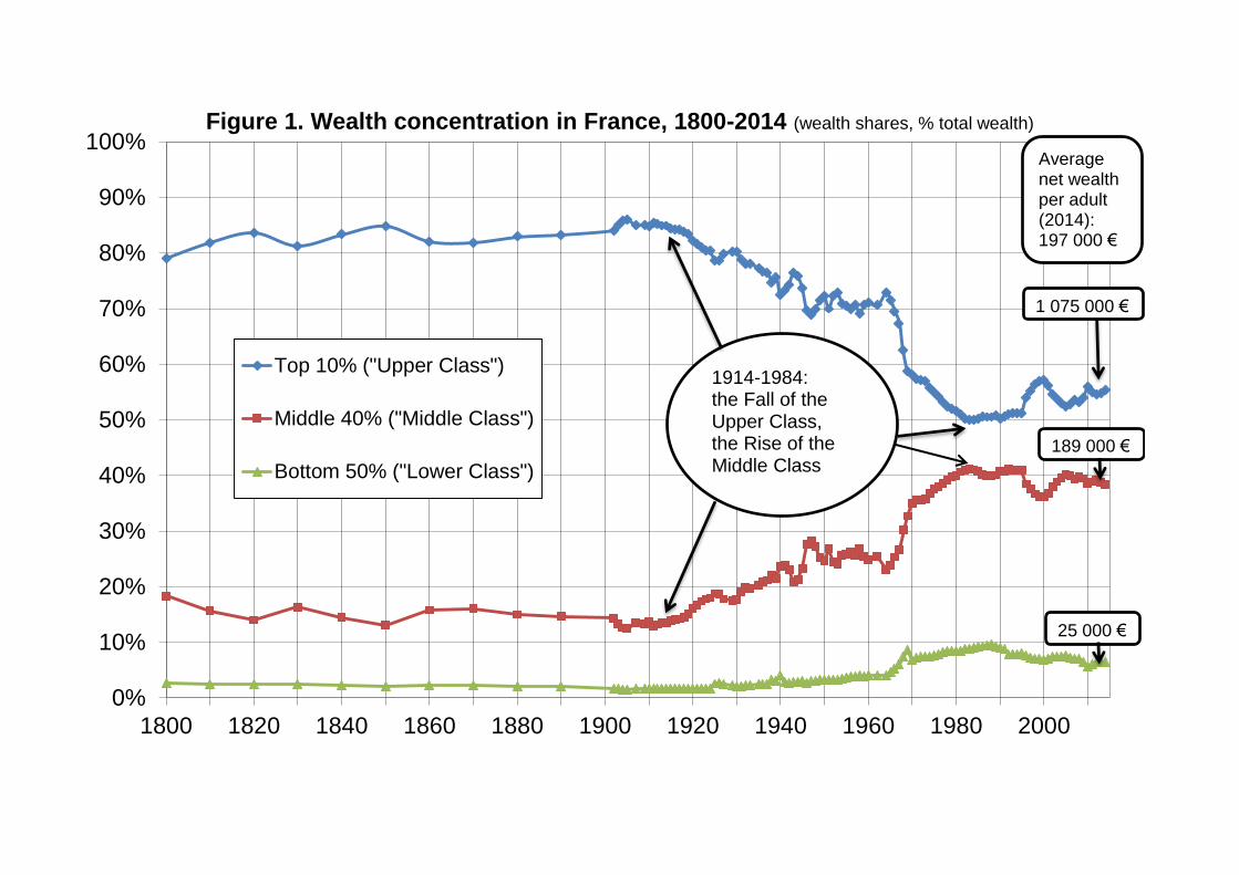
0%

10%

20%

30%

40%

50%

60%

70%

80%

90%

100%

1800 1820 1840 1860 1880 1900 1920 1940 1960 1980 2000

Figure 1. Wealth concentration in France, 1800-2014 (wealth shares, % total wealth)

Top 10% ("Upper Class")

Middle 40% ("Middle Class")

Bottom 50% ("Lower Class")

1914-1984: the Fall of the Upper Class, the Rise of the Middle Class

1 075 000 €

189 000 €

25 000 €

Average net wealth per adult (2014): 197 000 €

10%

15%

20%

25%

30%

35%

40%

45%

50%

55%

60%

1800 1820 1840 1860 1880 1900 1920 1940 1960 1980 2000

Figure 2. Top wealth shares in France, 1800-2014 (% total wealth)

Top 1%

Top 10-1%

683 000 €

4 614 000 €

Average net wealth per adult (2014):

197 000 €

20%

25%

30%

35%

40%

45%

50%

55%

60%

65%

70%

75%

80%

85%

90%

95%

100%

1900 1910 1920 1930 1940 1950 1960 1970 1980 1990 2000 2010

Figure 3. Top 10% share: income vs wealth

Top 10% share (capital income)

Top 10% share (wealth)

Top 10% share (total income)

Top 10% share (labor income)

Distribution of total income, labor income, capital income and net wealth among adults. Equal-split-adults series (income and wealth of married couples divided by two).

0%

5%

10%

15%

20%

25%

30%

35%

40%

45%

50%

55%

60%

65%

1900 1910 1920 1930 1940 1950 1960 1970 1980 1990 2000 2010

Figure 4. Top 1% share: income vs wealth

Top 1% share (capital income)

Top 1% share (wealth)

Top 1% share (total income)

Top 1% share (labor income)

Distribution of total income, labor income, capital income and net wealth among adults. Equal-split-adults series (income and wealth of married couples divided by two).

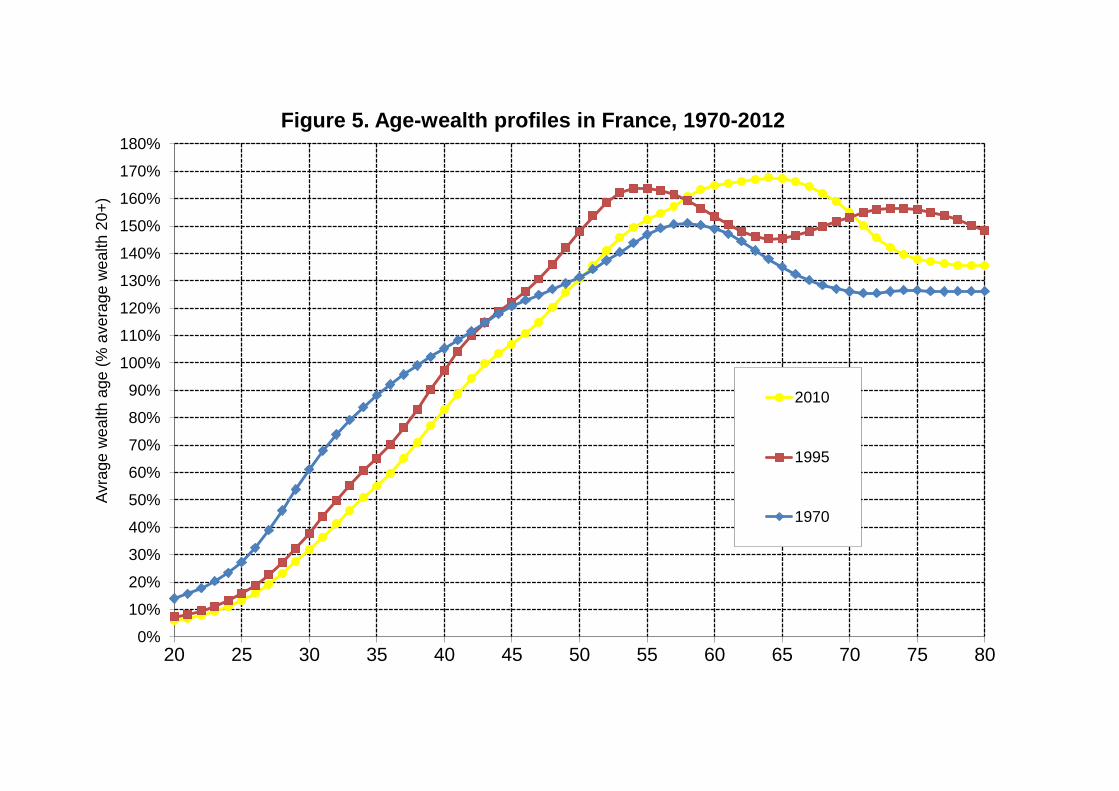
0%

10%

20%

30%

40%

50%

60%

70%

80%

90%

100%

110%

120%

130%

140%

150%

160%

170%

180%

20 25 30 35 40 45 50 55 60 65 70 75 80

Avra

ge

we

alth

age

(%

ave

rage

we

alth

20

+)

Figure 5. Age-wealth profiles in France, 1970-2012

2010

1995

1970

0%

10%

20%

30%

40%

50%

60%

70%

80%

90%

100%

1970 1975 1980 1985 1990 1995 2000 2005 2010

We

alth

sh

are

s (

% t

ota

l w

ea

lth

of

ea

ch

ag

e g

rou

p)

Figure 6. Wealth concentration by age group, France 1970-2012

Top 10% (all ages) Middle 40% (all ages) Bottom 50% (all ages)

Top 10% (20-39-yr) Middle 40% (20-39-yr) Bottom 50% (20-39-yr)

Top 10% (40-59-yr) Midle 40% (40-59-yr) Bottom 50% (40-59-yr)

Top 10% (60-yr+) Middle 40% (60-yr+) Bottom 50% (60-yr+)

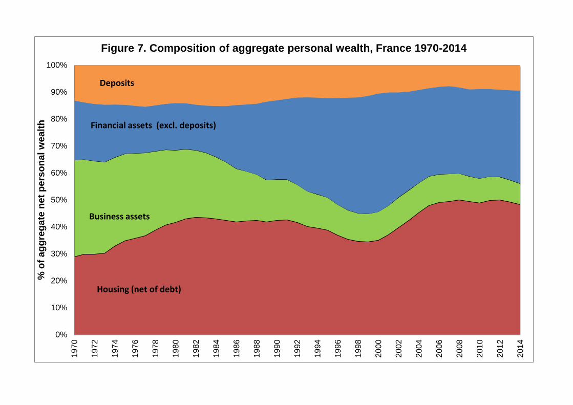
0%

10%

20%

30%

40%

50%

60%

70%

80%

90%

100%1

97

0

197

2

197

4

197

6

197

8

198

0

198

2

198

4

198

6

198

8

199

0

199

2

199

4

199

6

199

8

200

0

200

2

200

4

200

6

200

8

201

0

201

2

201

4

% o

f a

gg

reg

ate

ne

t p

ers

on

al w

ea

lth

Figure 7. Composition of aggregate personal wealth, France 1970-2014

Deposits

Housing (net of debt)

Business assets

Financial assets (excl. deposits)

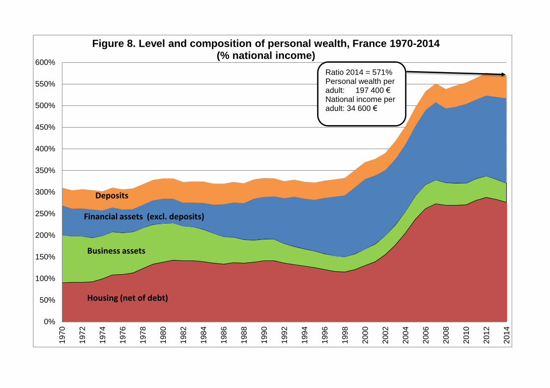
0%

50%

100%

150%

200%

250%

300%

350%

400%

450%

500%

550%

600%1

97

0

197

2

197

4

197

6

197

8

198

0

198

2

198

4

198

6

198

8

199

0

199

2

199

4

199

6

199

8

200

0

200

2

200

4

200

6

200

8

201

0

201

2

201

4

Figure 8. Level and composition of personal wealth, France 1970-2014 (% national income)

Deposits

Housing (net of debt)

Business assets

Financial assets (excl. deposits)

Ratio 2014 = 571% Personal wealth per adult: 197 400 € National income per adult: 34 600 €

0%

10%

20%

30%

40%

50%

60%

70%

80%

90%

100%

P0-10 P10-20 P20-30 P30-40 P40-50 P50-60 P60-70 P70-80 P80-90 P90-95 P95-99 P99-99.5

P99.5-99.9

P99.9-100

Figure 9. Asset composition by wealth level, France 2012

Housing (net of debt)

Business assets

Financial assets (excl. deposits)

Deposits

2 450 €€ 23 000 € 111 000 € 198 000 € 497 000 € 2 368 000 € 15 650 000 €

0%

5%

10%

15%

20%

25%

30%

35%

40%

45%1

97

0

197

2

197

4

197

6

197

8

198

0

198

2

198

4

198

6

198

8

199

0

199

2

199

4

199

6

199

8

200

0

200

2

200

4

200

6

200

8

201

0

201

2

201

4

Figure 10. Decomposition of middle 40% wealth share (% aggregate wealth)

Deposits

Housing (net of debt)

Middle 40% personal wealth per adult : 189 000 € (2014)

Business assets

Financial assets (excl. deposits)

0%

5%

10%

15%

20%

25%

30%

35%1

97

0

197

2

197

4

197

6

197

8

198

0

198

2

198

4

198

6

198

8

199

0

199

2

199

4

199

6

199

8

200

0

200

2

200

4

200

6

200

8

201

0

201

2

201

4

Figure 11. Decomposition of top 1% wealth share (% aggregate wealth)

Deposits

Housing (net of debt)

Top 1% personal wealth per adult :

4 614 000€ (2014)

Business assets

Financial assets (excl. deposits)

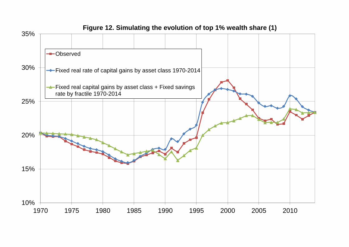
10%

15%

20%

25%

30%

35%

1970 1975 1980 1985 1990 1995 2000 2005 2010

Figure 12. Simulating the evolution of top 1% wealth share (1)

Observed

Fixed real rate of capital gains by asset class 1970-2014

Fixed real capital gains by asset class + Fixed savingsrate by fractile 1970-2014

10%

15%

20%

25%

30%

35%

1970 1975 1980 1985 1990 1995 2000 2005 2010

Figure 13. Simulating the evolution of top 1% wealth share (2)

Observed

Fixed real rate of capital gains by asset class 1970-2000

Fixed real capital gains by asset class + Fixed savingsrate by fractile 1970-2000

-5%

0%

5%

10%

15%

20%

25%

30%

35%

1970 1975 1980 1985 1990 1995 2000 2005 2010

Figure 14. Synthetic saving rates by wealth group

Top 10%

Middle 40%

Bottom 50

0%

2%

4%

6%

8%

10%

12%

1970 1975 1980 1985 1990 1995 2000 2005 2010

Figure 15. Flow returns by wealth group (before all taxes)

Top 1%

Top 10-1%

Middle 40%

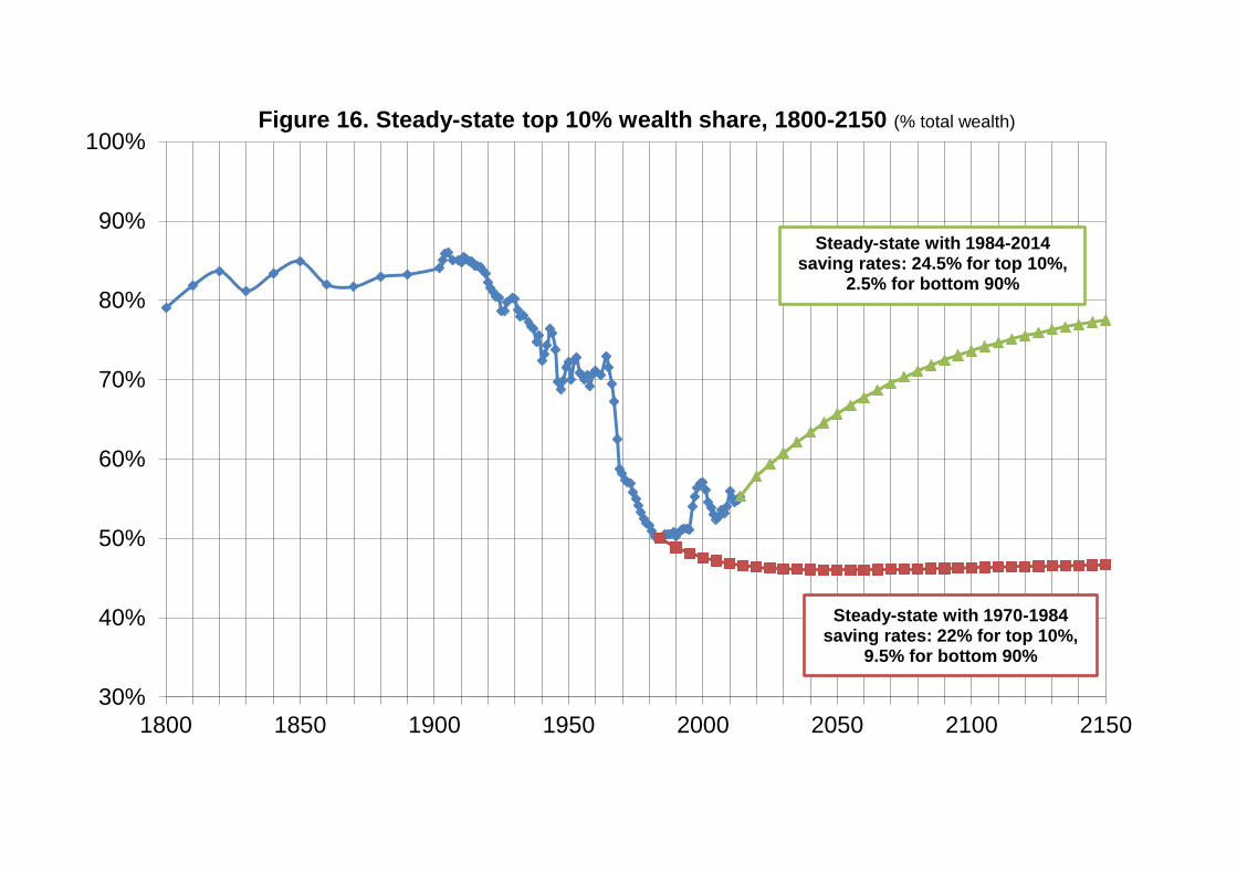
30%

40%

50%

60%

70%

80%

90%

100%

1800 1850 1900 1950 2000 2050 2100 2150

Figure 16. Steady-state top 10% wealth share, 1800-2150 (% total wealth)

Steady-state with 1984-2014 saving rates: 24.5% for top 10%,

2.5% for bottom 90%

Steady-state with 1970-1984 saving rates: 22% for top 10%,

9.5% for bottom 90%

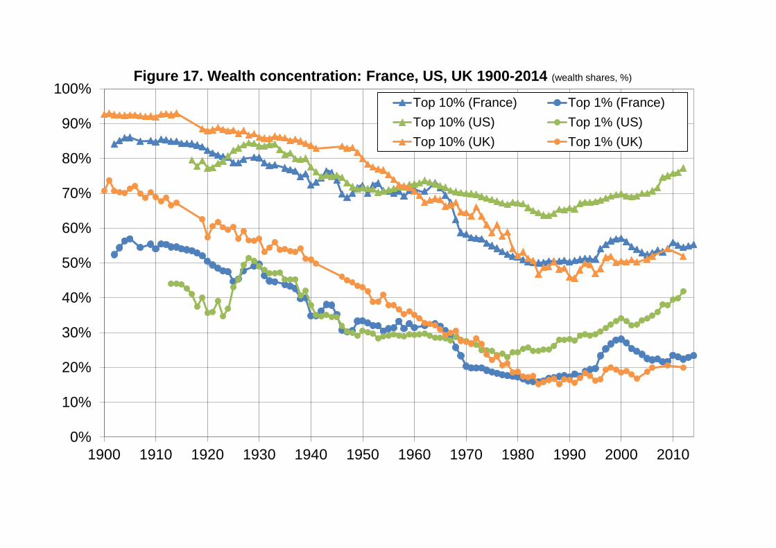
0%

10%

20%

30%

40%

50%

60%

70%

80%

90%

100%

1900 1910 1920 1930 1940 1950 1960 1970 1980 1990 2000 2010

Figure 17. Wealth concentration: France, US, UK 1900-2014 (wealth shares, %)

Top 10% (France) Top 1% (France)

Top 10% (US) Top 1% (US)

Top 10% (UK) Top 1% (UK)

1

Accounting for Wealth Inequality Dynamics:

Methods, Estimates and Simulations for France (1800-2014)

Data Appendix

Bertrand Garbinti, Jonathan Goupille-Lebret, Thomas Piketty *

First Version: July 12, 2016

Last Revised: January 27, 2017

This data appendix provides methodological details and complete data series for our

paper “Accounting for Wealth Inequality Dynamics: Methods, Estimates and

Simulations for France (1800-2014)”. It is supplemented by a set of data files and

computer codes (GGP2016Wealth.zip).

*We are grateful to Facundo Alvaredo, Emmanuel Saez, Daniel Waldenström and Gabriel Zucman for numerous conversations. The research leading to these results has received funding from the European Research Council under the European Union's Seventh Framework Programme, ERC Grant Agreement n. 340831. This work is also supported by a public grant overseen by the French National Research Agency (ANR) as part of the « Investissements d’avenir » program (reference : ANR-10-EQPX-17 – Centre d’accès sécurisé aux données – CASD). Updated files and series are available on the WID.world website (World Wealth and Income Database): http://WID.world. Contacts: Garbinti (Banque de France, Crest): bertrand.garbinti@ensae.fr; Goupille-Lebret (Paris School of Economics, GATE-LSE): jonathan.goupille@ens.fr; Piketty (Paris School of Economics): piketty@psemail.eu. This paper presents the authors’ views and should not be interpreted as reflecting those of their institutions.

2

Appendix A. Benchmark unified wealth distribution series (1800-2014)

Appendix B. Detailed series using income capitalization method

Appendix C. Detailed series using estate multiplier method

Appendix D. Reconciliation between the two methods (1984-2010)

Appendix E. Simulations: models and results

Appendix F. Reconciliation using household wealth surveys

Appendix G. Reconciliation using annual wealth tax data

Appendix H. Reconciliation using billionaire rankings and rich lists

3

This Data Appendix has two main purposes: to provide all relevant details on the data

sources and methods we use in this research, and to provide complete data series

on wealth inequality dynamics.

The Appendix is organized as follows. In Appendix A, we present complete tables

and additional figures of our benchmark unified wealth distributions series for the

period 1800-2014. These series are obtained by combining different data sources

and methods over time.

All data files, computer codes, additional series and robustness checks regarding the

different methods used in our benchmark series are presented in Appendices B to D.

Appendix B presents the mixed income capitalization-survey method used to

estimate the distribution of wealth for the 1970-2014 period. Appendix C relates to

the estate multiplier approach over the 1800-1970 period. Appendix D offers a

reconciliation between estate-multiplier and income-capitalization estimates for the

1984-2010 period. Appendix E relates to the formula and simulations of long-run,

steady-state level of wealth concentration. It includes the complete developments of

the steady-state formula as well as additional simulations.

Finally, Appendices F to H offers a reconciliation of our benchmark series with other

sources of wealth data such as household wealth surveys (Appendix F), wealth tax

data (Appendix G) and rich lists (Appendix H).

This Appendix is supported by several series of Excel and PDF files as well as

computer codes that contain and present our complete wealth inequality series. The

directory GGP2016Wealth.zip is organized as follows. For each section of the

Appendix, there is a folder called GGP2016WealthAppendixX (with X=A,…,H). Each

of these folders contains all the relevant materials (Excel files, computer codes, etc.)

as well as a ReadMe file presenting these elements. The Excel files are called

GGP2016WealthAppendixX.xlsx and contain all tables and figures relatives to the

section and excluded from the main text for the sake of conciseness. These Excel

files can be supplemented by a DataFiles folder including all computer codes and raw

data used to produce the wealth inequality series.

4

Appendix A. Benchmark unified wealth distribution series (1800-2014)

Appendix A includes additional tables and figures of our benchmark unified wealth

distribution series. The corresponding Excel file (GGP2016WealtAppendixA) reports

wealth shares, wealth thresholds and Pareto coefficients for synthetic wealth groups

(TA1) as well as for the complete 127 generalized percentiles (TA2). It includes also

supplemental figures on wealth concentration in France (FA1 to FA3), on the

comparison of France with the US (FA4 and FA5) and on the average wealth/national

income ratio by wealth fractile (FA6 to FA8).

5

Appendix B. Detailed series using income capitalization method

Appendix B relates to the estimation of wealth distribution series broken down by

percentile, age, gender and asset categories over the 1970-2014 period. The series

are derived from a mixed method based on income capitalization and imputations

from wealth surveys and housing surveys. First, we present in this section the

different files included into the directory GGP2016WealthAppendixB. Then, we

present the raw data sources used (income tax micro-files). Finally, we detail the

different steps of the mixed income capitalization method and the robustness checks.

Section B.1. Files description

The Excel File GGP2016WealthAppendixB includes the main appendix tables and

figures for detailed wealth series over the period 1970-2014. It presents tables on

wealth shares and wealth composition (TB1 to TB4b) ; on the determinants of wealth

inequalities by wealth group such as rates of return, real rates of capital gains, saving

rates and labor income shares (TB5a to TB13) ; on other series relative to inter and

intra generational wealth inequality and robustness checks (TB20 to TB22). The file

reports also supplemental figures on wealth concentration (FB1 to FB2), flow returns

and rates of capital gains by wealth group (FB3 to FB6), robustness checks (FB7 to

FB12), wealth composition by wealth group (FB20 o FB28) and Pareto coefficients

(FB30 to FB35). An index is included in the file for a complete list of tables and

figures.

All the tables and figures are derived from synthetic files extracted from micro-files.

These synthetic files fall into three categories. The first category of files is called

“gperc” and includes for each gender and each of the 127 g-percentiles of net wealth

among adults: lower wealth threshold, bottom average wealth, top average wealth

and g-percentile average wealth. The second category is called “dperc”. It reports

wealth shares by decile1 and gender along with a decomposition of wealth by asset

categories. Finally, the last category of files reports average wealth broken down by

age, gender and wealth groups. These synthetic files are included into the folder

1 The last decile is split into 5 categories P90-95, P95-99, P99-99.5, P99.5-99.9 and P99.9-100.

6

DataFiles along with all computer codes and files that we use to produce

homogenous wealth and income series out of income tax returns from 1970 to 2014

using capitalization method. (see ReadMe file in directory).

Section B.2. Description of data sources (income tax micro files)

As described in the core of the paper, the estimation of the wealth distribution for the

1970-2014 period is based on micro-files of income tax returns. These micro-files

have been produced by the French Finance Ministry since 1970 and fall into two

categories: “Enquête Revenus Fiscaux” (Tax Income surveys, hereafter: ERF

surveys) and “Echantillons Légers et Lourds” (hereafter: samples of income tax

returns).

We use the first series of ERF surveys produced jointly by Insee2 and the tax

administration every 5 years from 1970 to 1990.3 The surveys describe the socio-

demographic structure of approximately 40,000 tax units along with all the

information reported in their income tax returns (containing different sources of

taxable income and income tax).

In addition, we have access to large samples of income tax returns edited each year

by the tax administration since 1988. These files include 40,000 tax units from 1988

to 1993 (Echantillon léger) and about 400,000-500,000 tax units per year since 1994

(Echantillon lourd). These micro-files are stratified by taxable income brackets with

large oversampling at the top (they are exhaustive at the very top). Since 2010 we

also have access to exhaustive micro-files, including all tax units, i.e. about 37 million

tax units in 2010-2012.

2 Insee stands for Institut National de la Statistique et des Études Économiques and is the national

institute in charge of the production, the analysis and the diffusion of official statistics in France. 3 The first series of ERF surveys was edited eight times since 1956 (1956, 1962, 1965, 1970, 1975,

1979, 1984 and 1990). The first ERF of 1956, 1962 and 1970 are not available anymore. The Tax Administration was responsible for filling the data related to tax income, while Insee was in charge of the statistical data processing. The updated version of these surveys are now called The Tax and Social Incomes Survey (ERFS). They are annual and match information from Labor Force surveys with income tax returns and social benefits perceived. See description of Tax Income Survey/ERF and Tax and Social Income Survey/ERFS on Insee website.

7

Finally, we also have access to income tax tabulations, which have been produced

by the French Finance Ministry since the creation of income tax in France in 1914.

They report the number of taxpayers and total income for a large number of income

brackets. In principle, income capitalization method could also be used with tabulated

income tax data broken down by income sources prior to 1970 (see Piketty 2001,

Appendix B, Table B16). However, these tabulations by income categories suffer

from a number of limitations4, so that we prefer to use the income capitalization

method as our benchmark method for the 1970-2014 period (when we have access

to micro-files of income tax returns), and to adopt the estate multiplier method (based

upon inheritance tax returns) as our benchmark method prior to 1970.5

Section B.2.1. Harmonization of micro files

From these different databases, we unify the concepts and names of our variables of

interest which include income and demographic variables for each member of the tax

unit.

Income variables: labor and replacement incomes (wages, unemployment

benefits and pensions), financial incomes (dividends, interests, life

insurance income), self-employment income, real (non-imputed) rents

Demographic variables: age of all members of the fiscal household and

sex of the head of the fiscal household.6

As stated before, the samples of income tax returns are large (recent ones contain

500,000 fiscal units) and exhaustive at the very top. In contrast, ERF surveys are of

smaller size with approximately 45,000 fiscal units. The ERF surveys are

4 Generally speaking, the main limitation of income tax tabulations is that prior to 1985 they only cover

tax units that are subject to positive income tax. Another specific limitation of tabulations by income categories is that prior to 1945 they only cover a limited number of years (namely, 1917, 1920, 1932, 1934, 1936 and 1937; they then become annual in 1945). In contrast, inheritance tax tabulations cover the entire distribution of wealth (whether the estate is taxed), and they cover many more years prior to 1945. Full details on income tax tabulations and the way we exploit them are given in our companion paper Garbinti, Goupille-Lebret and Piketty (2017, Appendix D). 5 As there are no inheritance tax tabulations during the period 1914-1924 and 1965-1969, we

complete the missing years by using data on top capital incomes from income tax tabulations. 6 We assume that the second member of the couple has the opposite sex of the head of the

household. This assumption is relatively reasonable since couples of the same sex represents 0.6% of all couples (Buisson and Lapinte, 2013). We impute randomly the sex of the dependents. Again, this imputation has no consequences on our results as adult dependents represent less than 4% of the population, are very young (24 years old in average) and have very low income.

8

representative of the French population as a whole but not necessarily of the highest

income earners. To check this, we compare the upper part of the income distribution

from the ERF surveys with the income tax tabulations. In particular, we check the

consistency of the income thresholds, the average incomes and their decomposition

by income categories (rents, financial income, self-employment income, and labor

income) for different income groups at the top of the distribution (P90-95, P95-99,

P99-99,5, P99,5-99,9 and P99,9-100) .

The comparison between the ERF surveys and the tabulations reported in Piketty

(2001) shows that average incomes by income group are almost identical but the

compositions of income differ strongly for the first three surveys. Indeed, for years

1970, 1975 and 1984, labor incomes and rents are overrepresented in the top decile

income of ERF surveys, while financial and self-employment incomes are

underrepresented. In contrast, we find that average incomes and income

compositions are identical for years 1988 and 1990 between the tabulations and the

samples of income tax returns (Echantillon Léger). We then conclude that the

differences we observe for the oldest ERF surveys may be due to a lack of statistical

precision at the top of the income distribution. To tackle this issue, we correct the

composition of the top 10% income group from the ERF surveys using the income tax

tabulations.7

Section B.2.2. Individualization of micro files: from tax units to individual units

While the micro-files are at the tax unit level, our unit of interest is the individual level.

We exploit the fact that age and gender are reported for each member of the fiscal

household to fully individualize our data. More precisely, we create one observation

for each member of the tax units older than 20 years old. Labor, replacement and

self-employment incomes are already reported at the individual level. In contrast,

financial income and rents are reported jointly for the entire fiscal household. In this

case, we assume an equal split among spouses. By convention, dependents earn no

7 More precisely, we split individuals into 6 income groups in the ERF surveys (P0-P90, P90-95, P95-

99, P99-99.5, P99.5-99.9 and P99.9-100). Then we adjust each individual income and their components such as the adjusted average income for the different income groups matches those from income tax tabulations. We then follow an iterative process to adjust the income composition of the different income groups in the ERFS survey (rents, labor, financial and mixed incomes) to the appropriate one from the income tax tabulations.

9

financial income and no rent. Note that in France, adult children are supposed to

report personally their incomes. But, when they depend on their parents’ financial

support, the parents can report them as dependents until they are 21 years old (at

January the 1st) or 25 years old if they are pursuing an education. It is generally

interesting for parents to report them because it leads to a tax reduction (thanks to

the “quotient familial”).

After individualizing the tax unit (and particularly the dependents), the number of

young adults aged less than 25 included in our data appears to be slightly less

important than in the census data. It may be due to the fact that the date of birth is

not always reported for each dependent children. We then add the missing

individuals aged 20-25 years with zero income, using the demographic margins by

age and gender from Insee. At this stage, our micro-files are fully individualized and

consistent with the French demographic structure for each year.

Section B.3. From taxable income to DINA capital income and wealth

The general idea behind the income capitalization method is to recover the

distribution of wealth from the distribution of capital income flows. In its simplest form,

the method relies on the assumption of fixed rates of return by asset class (see e.g.

Atkinson and Harrison, 1978, and Saez and Zucman, 2016). Unfortunately, all assets

do not yield taxable income and we need to adapt the capitalization method in order

to impute these assets.

Here we split wealth into seven different categories of assets and corresponding

capital income flows: housing assets – split into owner-occupied housing and tenant-

occupied housing assets – as well as their corresponding debts, business assets,

financial assets – split into equities, bonds and loans, deposits and savings accounts,

and life insurance and pension funds (see Appendix A from our companion paper

Table A20 for wealth and A13 for income). Four different categories of capital income

are reported into the income tax returns: interests8, dividends, self-employment

8 Some kinds of interests are automatically taxed at “Prélèvement libératoire forfaitaire” (PLF) that is a

withholding tax. Changes in the way these interests are reported into the income tax returns create artificial jumps in series for years 1995 and 1999. In the present version we do not use reported

10

income and tenant-occupied rental income. For these capital incomes, we estimate

the corresponding stock of assets by using the income capitalization method. More

specifically, we first compute the aggregate rate of return for each asset class ri by

dividing the total reported returns in the income tax returns Ri by the reported stock Ai

in the national accounts. We can then obtain the stock of the different assets by

dividing each capital income components reported at the individual level by the

corresponding aggregate rate of return ri.

Section B.3.1. Imputation based on household surveys

We complement the capitalization method with imputations based on household

surveys (wealth and housing surveys) that present the huge advantage to report both

income and wealth.9 The imputations allow us to estimate the stock of assets that do

not generate taxable income flows, namely owner-occupied housing, life insurance,

and deposits (including currency and saving accounts). The imputation procedure is

the following.10

First, in the surveys, we define groups according to three dimensions: age, financial

income, and labor and replacement income. For example, we define approximately

200 groups for the imputation of owner-occupied housing asset. We first split the

sample into 10 age groups (< 25 ; 25-30 ; 31-39 ; 40-49 ; 50-54 ; 55-60 ; 61-65 ; 66-

70 ; 71-80 ; > 80). We then divide each age group into 4 percentile groups of financial

income (P0-50 ; P50-90 ; P90-99 ; P99-100). Finally, we split again each of these 40

groups (10 age groups *4 groups of financial income) into 5 percentile groups of

labor and replacement income (P0-25, P25-50, P50-75, P75-90, P90-100).

Second, for each group and each kind of asset to be imputed (owner-occupied

housing, deposits, and life insurance), we both compute an extensive (the proportion

of individuals holding the asset considered) and an intensive (share of the total asset

owned by the group) margins. For the intensive margin of the owner-occupied

information about these specific interests. When computing bonds and loans, we then assume that they are proportional to the interests taxed according to the regular income tax schedule. 9 Since 2010, the incomes reported in the wealth surveys directly come from the income tax returns.

10 See the Stata codes in DataFiles/Capitalization method/Imputation in Appendix B for a complete

and exhaustive description of the imputation method.

11

housing, we compute the share of total gross housing owned by the group along with

the debt ratio (Debt/ Gross value of the owner-occupied housing). For instance, if

80% of the individuals in a group owns a primary residence, the total gross value of

the housing asset this group owns represents 0.5% of the total value reported in the

survey and their mortgage represent 50% of the gross value of their housing asset,

then the extensive margin is 80%, the intensive one is 0.5% and the debt ratio is

50%.

Third, in our income tax micro files, we define groups according to the same

dimensions (age, financial and labor incomes). Then, within each group, we randomly

draw tax units who own the asset accordingly to the extensive margin computed for

the asset and the group considered. To go back to our former example, it means that

80% of the group will be considered as owning the asset. The intensive margin is

then used to impute the asset amount within the asset holders of this group. In our

former example, it means that the asset-holders (who represent 80% of the

considered group) will be supposed to hold globally 0.5% of the 4,484 billion euros

that the gross owner-occupied housing asset represents in 2010. If the group

represents 100,000 tax units, it means that each of the 80,000 tax units who own this

asset will hold 0.5%*4,484 billions/80,000 that is 280,000 euros of gross owner-

occupied housing. The remaining 20,000 tax units of this group won’t hold any

housing asset. Finally, as the debt ratio is equal to 50% in our example, the mortgage

associated to the housing asset will be equal to 140,000 euros.

We should highlight that the imputations take place at the tax unit level. For life

insurance and owner-occupied housing, income and stocks are then equally split

among couples.11 In contrast, deposits can be owned by all members of the tax unit

(dependents and couples). For this asset, we have also computed an additional

statistic for each group in the surveys corresponding to the fraction of deposits owned

by the dependents. We therefore allocate the fraction of deposits owned by each

member of the tax unit.

11

The imputation at the tax unit level allows for consistency of wealth among the spouses or partners that should necessarily have the same wealth.

12

Finally, we estimate the different components of capital income by simply multiplying

each asset by the corresponding economic rate of return (see Table A24 from

Appendix A of our companion paper for the rates of return by asset computed from

national accounts).

Section B.4. Robustness checks

To assess the sensitivity of our mixed capitalization method, we conducted several

robustness checks (see corresponding figures and tables in the Excel file of

Appendix B).

Section B.4.1. Imputation of owner-occupied housing assets

We first investigate the sensitivity of our results to the imputation of owner-occupied

housing assets. In our benchmark scenario, the imputation method is based on

housing surveys (1970, 1973, 1978, 1984, 1988, 1992) and wealth surveys (1992,

1998, 2004 and 2010).

Although Housing surveys are also available after 1992 (1992, 1996, 2002, 2006 and

2010), we tend to favor wealth surveys over housing surveys for the recent period.

Indeed, wealth surveys include a more complete description of the different sources

of income (capital, labor...), the present value of owner-occupied housing assets and

the associated debts at the time of the survey.12 This change of surveys used before

or after 1992 is likely to introduce two kind of comparability issues. First, the

imputation method implemented is more sophisticated when using wealth surveys

instead of housing surveys.13 Second, the distribution of owner-occupied housing and

12

In the housing surveys, only total income is reported. Although housing occupation status is reported for all households, the value of the housing assets is asked only to home owners having bought their housing assets less than 4 years before the time of the survey. In this case, the value reported corresponds to the value of the housing assets at the time of the purchase rather than at the time of the survey. In addition, individuals are asked about their total debt rather than the mortgage associated to their housing assets. 13

The imputations groups are defined according to three dimensions (age, financial income, and labor and replacement income) when using wealth surveys against two dimensions (age and total income) when using housing surveys. Consequently, there are 200 imputations groups when using wealth surveys against 63 groups when using housing surveys.

13

the associated debts is better described and more accurate in the wealth surveys

than in the housing surveys.122

We investigate the potential comparability issues implied by the use of wealth

surveys instead of housing surveys after 1992 in Figures B7 to B9 and Table B22.

The first robustness check assesses the sensitivity of our results to the imputation

method. In this scenario, we apply the simplified imputation procedure based on two

dimensions (age and total income) to the complete period rather than only to the pre-

1992 period in the baseline scenario. In the second robustness check, we use the

housing surveys for the complete period 1970-2012. Figures B7 to B9 show that

these changes have no significant effect on our results.

Section B.4.2. Alternative imputations of financial assets

We then investigate the sensitivity of our results to different imputation methods for

financial assets. First, we impute life insurance proportionally to taxable interests and

dividends rather than relying on imputation methods based on wealth surveys.14

Second, we capitalize all financial incomes (interests from debt assets or savings

accounts, life insurance income, dividends) using a unique rate of return.15

Note that both sensitivity checks are upper bound scenarios in terms of wealth

concentration. Indeed, bonds and equities are strongly concentrated at the top of the

distribution and benefit from higher returns than deposits and saving accounts that

are concentrated at the bottom. Using the same capitalization factor to all financial

incomes will therefore decrease the estimated value of the low-return asset and

increase the estimated value of the high-return asset and therefore lead to a more

important level of wealth concentration. For similar reasons, imputing life insurance

proportionally to taxable interest and dividends will overestimate the level of wealth

concentration.

14

See section B.3 above for the description of the imputation method used in the baseline scenario. 15

Interests from saving accounts and life insurance income are still imputed based on household surveys but the corresponding asset is recovered using an aggregate rate of return common to all financial income and defined as the ratio of capital income to financial assets reported in the national accounts.

14

Table B22 and Figures B10 to B12 report the level of wealth concentration depending

on the imputations of financial assets used. The different sensitivity checks imply a

slightly more important level of wealth concentration but the different trends as well

as our different results and interpretations remain the same.

Section B.4.3. Capitalization of taxable interests and dividends

In our benchmark series, we jointly capitalize taxable interests and dividends to

recover equities and bonds. We then reclassify them into equities or bonds

proportionally to the respective importance of interests and dividends in the individual

income. As it turns out, the frontier between interests and dividends reported in the

income tax returns can be fuzzy and has changed over time. For instance, some

capital incomes from mutual funds (FCP and OPCVM) were classified as “interests”

(case TS from income tax returns) and switched to the “dividends” category (case DC

from income tax returns) since 2005. This artificial change leads to a break in our

fiscal series of dividends and interests that is our main motivation to capitalize them

together. However, as a robustness check, we decide to test a variant where

interests and dividends are capitalized separately after correcting for the artificial

change occurring in 2005.16 This allows us to test whether our conclusions are

impacted by this change. Results are presented in Table B22 and Figures B10 to

B12. Again, the overall impact on wealth distribution series is very limited.

Section B.5. Miscellaneous remarks

Section B.5.1. Interpolation for missing years

As described in Section B.2, micro samples of income tax returns are not available

on an annual basis from 1970 to 1990. We interpolate the missing years 1971-1974,

1976-1978, 1980-1983, 1985-1987 and year 1989 by using annual aggregate series

16

Before 2005, the case TS in the income tax returns includes interest along with capital income from mutual funds that should be reported in the case DC corresponding to the dividends. For each year before 2005, we estimate the share of capital income from mutual funds reported in case DC by using the repartition key defined as the change observed from 2004 to 2005 between the fiscal case TS and the case DC. We assume then that, between these two consecutive years and between these two fiscal cases, the essential difference comes from the change in the way households report these amounts and not from a major portfolio change. We think this is the most plausible assumption.

15

by asset categories from national accounts and by assuming linear trends in within-

asset-class distribution. The main advantage of this interpolation method is that it

allows to take into account differential shocks between assets, while remaining 100%

consistent with the evolution of the aggregate stock of assets (as defined in the

national accounts) over time.

We illustrate our interpolation method with the following example. Let’s note

𝑆ℎ𝑖𝑗𝑡

the share of the asset i hold by the wealth group j at time t in proportion of the

aggregate private wealth and 𝑆ℎ_𝑡𝑜𝑡𝑖𝑡 the proportion of the asset i at time t into the

aggregate private wealth as reported in the national accounts. For a given missing

year t from 1970 to 1975, we have:

𝑆ℎ𝑖𝑗𝑡 = (

𝑆ℎ𝑖𝑗1970

𝑆ℎ_𝑡𝑜𝑡𝑖1970 + [

𝑆ℎ𝑖𝑗1975

𝑆ℎ_𝑡𝑜𝑡𝑖1975 −

𝑆ℎ𝑖𝑗1970

𝑆ℎ_𝑡𝑜𝑡𝑖1970] ∙

𝑡 − 1970

1975 − 1970) ∙ 𝑆ℎ_𝑡𝑜𝑡𝑖

𝑡

As an alternative strategy, we also used annual income tax tabulations (broken down

by income categories) and found that this makes very little difference.

Section B.5.2. Computation of saving rates, rates of return and capital gains by

wealth group

Tables B5a to B8 report saving rates, rates of return and rates of capital gains by

wealth group.

For each wealth group, the rates of returns are computed by weighting each asset-

specific rate of return – such as reported in the national accounts17 – by the

proportion of each asset in the wealth of the group. We follow the same methodology

to compute the rates of capital gains by wealth group.

17

See Tables A23-A25 of the Appendix A of our companion paper for the rates of return and capital gain by asset computed from national accounts.

16

The synthetic saving rate is defined in the same way as Saez and Zucman (2016)

(See discussion in the core of the paper). We first define the following transition

equation:

𝑊𝑡+1𝑝 = (1 + 𝑎𝑡)(1 + 𝑞𝑡

𝑝)[𝑊𝑡𝑝 + 𝑠𝑡

𝑝 ∙ 𝑌𝑡𝑝]

With: 𝑊𝑡𝑝

t, 𝑊𝑡+1𝑝

= average wealth of group p at time t and t+1 (for instance, group p

could be the top 10% wealth group)

𝑌𝑡𝑝 = average income of group p at time t

𝑞𝑡𝑝 = average real rate of real capital gains of group p from t to t+1 (real capital gains

are defined as the excess of average asset price inflation, given average portfolio

composition of group p, over consumer price inflation)

𝑎𝑡 = average asset price inflation

𝑠𝑡𝑝 = synthetic saving rate of group p at time t

We can then compute the synthetic saving rate:

𝑠𝑡𝑝 =

𝑊𝑡+1𝑝

(1 + 𝑎𝑡)(1 + 𝑞𝑡𝑝)−𝑊𝑡

𝑝

𝑌𝑡𝑝

Section B.5.3. Age-Wealth profiles

We present complete series of age-wealth profiles from 1970 to 2012 in Table B21.

The series are obtained by a local mean-smoothing also known as the Nadaraya-

Watson estimator (1964)18.

18

That is in 𝑥: ∑𝐾ℎ𝑥(𝑥−𝑥𝑖)

∑ 𝐾ℎ𝑥(𝑥−𝑥𝑗)𝑁𝑗=1

𝑁𝑖=1 where 𝐾ℎ𝑥(𝑥 − 𝑥𝑖) stands for the kernel function (here epanechnikov)

and ℎ𝑥 the bandwidth around 𝑥 (chosen here by the standard rule-of-thumb as implemented in the Stata procedure lpoly).

17

Appendix C. Detailed series using estate multiplier method

In appendix C, we present our detailed wealth distribution series obtained by

applying the estate multiplier method to historical inheritance data available for

France over the 1800-1970 period.

The Excel File GGPWealthAppendixC includes the main appendix tables and figures

on long-term series of wealth concentration at death or among the living individuals.

The file reports also supplemental tables and figures documenting step by step how

wealth series are constructed starting from raw inheritance tabulations. An index is

included in the file for a complete list of tables and figures. The folder DataFiles

including all Stata-format and MatLab-format codes and files that we use to produce

homogenous historical g-percentile wealth. The folder OtherData includes

supplemental materials from other works used in this Appendix (including raw

inheritance tax tabulations from Piketty 2001).

We present in this section the different inheritance data sources used and the

different steps of the estate multiplier approach implemented in order to obtain the

wealth distribution series over 1800-1970.

Section C.1. Inheritance data sources in France (1800-2015)

The modern inheritance tax (“droits d’enregistrement”, i.e. “registration duties”) was

created as early as 1791 in France, as an important part of the new tax system

instituted by the French Revolution. The basic features of inheritance tax law were

unchanged since 1791, together with general rules to split inheritance between

siblings (Code Civil, 1804).

1802-1902 Period

Before 1902, the tax administration only published aggregate statistics on the value

of the estates broken down by very broad categories, e.g real (structures and

buildings) and personal (furniture, businesses, stocks, bonds, etc.) assets. Hopefully,

individual-level inheritance registers have been well preserved and are accessible to

18

researchers since 1800. These registers include detailed information about assets,

age, and gender, in principle for all decedents (irrespective of the level of their

wealth). One needs then to return to tax registers and collect its own sample of estate

tax returns to study wealth concentration.

For this period, we use inheritance tabulations based upon data collection of large

individual-level micro-samples of estates collected in Paris inheritance registers

(Piketty, Postel-Vinay and Rosenthal 2006) and of the provincial samples collected

by Bourdieu et al (2003, 2013) in the context of the TRA survey. These raw

inheritance tabulations are presented in Piketty, Postel-Vinay and Rosenthal (2006,

Table A3) and are available for selected years (1807, 1817, 1827, 1837, 1847, 1857,

1867, 1877, 1887 and 1902).19

1902-1964 Period

In 1902, the French inheritance tax became progressive and the tax administration

started compiling detailed tabulations reporting the number of decedents and amount

of their wealth for a large number of inheritance brackets. These tabulations are

consistent with the data collected in inheritance registers, and they are available on a

quasi-annual, exhaustive national basis between 1902 and 1964 (except for the

1914-1924 sub-period). They occasionally include supplementary breakdowns by

age brackets and asset categories. These raw inheritance tabulations are reported in

the Excel File GGP2016WealthAppendixC (Table C3).20

Section C.2. Long-run series using historical inheritance data (1800-1970)

We use the inheritance tabulations in order to compute our wealth distribution series

for the 1800-1970 period.21 This work is conducted in three steps. First, the

inheritance tabulations are pooled together for the complete period 1800-1964 and

homogenized. Second, we apply the Pareto interpolation techniques developed by

Blanchet, Fournier and Piketty (2017) to generate g-percentiles of inheritance from

19

See Piketty, Postel-Vinay and Rosenthal (2006) and the working paper version of 2004 for more details on the data and the methodology relative to the inheritance tax tabulations. 20

See Piketty (2001, Table J1) for a complete list of the references to the official publications from which these tabulations were copied.

19

inheritance tabulations. Finally, we estimate the distribution of adult wealth from the

distribution of inheritance using a refined estate multiplier method.

Section C.2.1. Correction for non-filers

The inheritance tax tabulation covered only the decedents for whom an inheritance

declaration was filled. Figures C1 to C3 of the Excel file report the number of

decedents and inheritance declarations in France over the period 1800 to 2010. The

annual number of adult decedents has generally been about 500-600 thousand

throughout the 1800-2010 period in France. The annual number of inheritance

declarations has generally been around 300-400 thousand (reflecting the fact that

decedents with very low net wealth do not get registered via an inheritance

declaration), except after the introduction of a large tax exemption in 1956, when it

briefly fell to less than 100 thousand. From 1800 to 1956, the fraction of adult

decedents covered by inheritance registers was therefore stable around 60%-70%.22

Although all inheritances were in principle subject to declaration and taxation, there

has always been some tolerance for very small net wealth holders (particularly within

the bottom 50% of the population, which typically owns less than 10% of aggregate

wealth).23 The tax exemption threshold introduced in 1956 led to a sharp reduction in

the number of declarations (although in principle declaration was still compulsory).

The threshold was under-indexed in the following decades, and the fraction of tax

filers gradually returned to earlier levels.

22

Note that TRA samples clearly show a slow decline of the proportion of adult decedents with inheritance declarations during the 19

th century (from about 70% in the early 19

th century to about 60%

by the end of the century), and that this seems strongly related to urbanization (property is less widespread in cities than in the country side). See Bourdieu et al (2003, figure 3; 2013, figure 11, p.147, tables 12-13, p.183). See also the very low proportion of inheritance declarations in Paris (Figure FC3 of the Excel file and Piketty, Postel-Vinay and Rosenthal (2006, 2014)). There is however some uncertainty about the exact proportion of inheritance declarations at the national level during the 19

th century, due in particular to the limited size of the TRA samples. Also note that TRA samples and

national tabulations are not entirely consistent on this issue. E.g. in 1902-1910 TRA samples find inheritance declarations for 56% of adult decedents, against 66% according to national tabulations. One possible interpretation would be that national tabulations include multiple individual declarations (when new information is added to the main declaration). See Bourdieu et al (2003, table 2 and ensuing discussion). If this was the case, then this would imply that national tabulations tend to under-estimate wealth concentration (as multiple declarations are more widespread for large estates). Another interpretation is that the TRA sample is not entirely representative. 23

See the Appendix of Piketty (2010) for a complete discussion of the estate tax data in France and tax filling requirement.

20

The only correction we made to the inheritance tax tabulations was to add non-filers

and their corresponding wealth. The corrected tabulations are presented in the Excel

File GGP2016WealthAppendixC (Tables C4 for 1902-1964 and C5 for 1807-1887).

These tables cover all adult decedents (filers and non-filers) and assume that the

ratio between non-filers and filers average wealth (znf) is equal to 2%.24

Table C6 reports the homogenized corrected inheritance tabulations 1807-1964 used

for generalized Pareto simulations. It depicts wealth thresholds and Pareto

coefficients by percentiles (P10, P50, P90, P95, P99, P99.5, P99.9 and P99.99). In

order to model explicitly for the functional form of the wealth distribution at the bottom

(see below for the description of the generalized Pareto simulations), we assume that

the wealth threshold of the first decile (P10) is set to fit post-1970 P10/P50 ratio

pattern.25 This assumption has no impact on wealth inequality as the wealth share of

the first decile has always been very low (less than 0.2% of total wealth).

Section C.2.2. Generating g-percentiles of inheritance from inheritance tabulations

We apply the generalized, non-parametric Pareto interpolation techniques developed

by Blanchet, Fournier and Piketty (2017) to the corrected inheritance tabulations

(Table C6) in order to estimate the complete distribution of wealth at death among

decedents over 1807-1964 period. Table C10 reports summary statistics for the

distribution of wealth at death, while Table C11 presents the detailed series by g-

percentiles (from P1 to P99.999). All the computer codes and files in MatLab and

Stata formats are gathered in the folder DataFiles of the Appendix C along with

ReadMe files presenting the different programs and output tables.

Note that we made two additional adjustments to obtain the complete series of wealth

at death during the 1807-1964 period. First, there is a discrepancy between fiscal

and economic flows of wealth at death due to legally tax-exempt assets and tax

evasion (see Table C2). The series were anchored to economic wealth at death

24

We also perform sensitivity checks with different values for znf and found that the impact on wealth inequality was relatively small. 25

P10 represents 7.7% of P50 in 1970 and ranges from 0.6% to 1.3% of average wealth over 1807-1964 period. See formulas in Tables C6 and C7 of the Excel file for more details.

21

instead of fiscal wealth at death by simply multiplying each amount by the ratio

between economic and fiscal wealth at death.26 Second, we estimate the distribution

of wealth for the years not covered by inheritance tax tabulation (1914-1924 and

1965-1969) using data on top capital incomes from income tax tabulations. Table

C7bis reports the index factors used for these periods.

Section C.2.3. Estimating the distribution of adult wealth from the distribution of

inheritance

Table C12 reports summary statistics for the distribution of wealth among adults,

while Table C13 presents the detailed series by g-percentiles. All details of the

methodology used in order to estimate the distribution of adult wealth from the

distribution of inheritance over the 1807-1964 period are given in the computer codes

and do-files. We use the same ratios as those used in Piketty 2014 (see xls files

Piketty2014Chapter10TablesFigures and Piketty2001TaxAnnexeJNov2015). These

ratios are taken from Piketty, Postel-Vinay and Rosenthal (2006) and are based upon

the application of the estate multiplier method to the micro-level files collected in

Parisian and national (TRA sample) inheritance archives between 1807 and 1964, as

well as the national tabulations by inheritance and age brackets published by the

Finance Ministry between 1902 and 1964.

It should also be noted that the ratios living/decedents obtained for top wealth shares

over the 1807-1964 period are typically larger than one (i.e. there is somewhat more

inequality when we include all living age groups together than when we only look at

decedents), but not that much larger than one (with ratios typically around 1.01 for

top 10% shares and 1.05 for top 1% wealth shares). Note also that Piketty (2014)

also uses the series from Piketty-Postel-Vinay-Rosenthal (2006) for 1984 and 1994

(based upon DMTG files and estate multiplier method) and from Landais-Piketty-

Saez (2011) for year 2010 (based upon income capitalization method). The series

used in the present paper for the entire 1970-2014 are based upon a mixed income

capitalization-wealth survey method and should be viewed as more precise.

26

We do not try to correct the distribution using differential factors by level of wealth. In absence of any external sources available at the micro level, it seems more reasonable to make a neutral assumption in terms of distribution.

22

23

Appendix D. Reconciliation between the two methods

(income capitalization and estate multiplier)

In our benchmark series, we combine wealth series derived from estate multiplier

approach using inheritance tax data from 1800 to 1970 with those obtained from a

mixed income capitalization-survey method using income tax returns and wealth

surveys from 1970 to 2014. The choice of the capitalization method over the estate

multiplier approach for the recent period is led by the fact that the former allows to

draw a more complete picture of wealth inequality. Indeed, the capitalization method

allows to estimate the joint distribution of income and wealth broken down by age,

gender and asset categories. However, we show in the present Appendix D that

wealth series derived from the capitalization method and the estate multiplier

approach depict similar results.

Section D.1. Files description

The Excel File GGPWealthAppendixD includes the main appendix tables and figures

for wealth series derived from the estate multiplier approach from 1984 to 2010.

Tables D1 to D5 report the demographic parameters (population, number of

decedents and mortality rate) and differential mortality rates (which in general could

vary by gender, age, time and wealth percentiles) used to apply the estate multiplier

approach. Wealth inequalities at death and for the overall population are also

reported (Tables D6 to D8) as well as sensitivity analysis (Tables D9 to D10, see

below). The file reports also supplemental figures on wealth concentration at death or

for the overall population along with a comparison of wealth series derived from the

capitalization method or the estate multiplier approach. An index is included in the file

for a complete list of tables and figures.

The folder DataFiles includes all codes and files that we use to produce homogenous

wealth series out of national micro-samples of inheritance tax returns (DMTG

microfiles) covering the years 1984, 1987, 1994, 2000, 2006 and 2010 (see ReadMe

file in directory).

24

Section D.2. Estate multiplier approach: General method

Section D.2.1. Mortality rates

The estate multiplier approach allows to recover the wealth distribution for the overall

population from the distribution of wealth at death. This approach stems from the

simple definition of the mortality rate m=D/L where m stands for the mortality rate, D

the number of decedents and L the number of living individuals. From the number of

decedents, it is thus easy to compute the number of living: L = D/m. We can therefore

recover the wealth distribution among the living from micro samples of inheritance tax

returns by simply reweighting each decedent by the inverse of the mortality rate.

However, this method relies on the assumption that death can be seen as an

exogenous event.

It is thus of concern to know to what extent death is purely exogenous or if it is

correlated with some characteristics. Indeed, the probability of dying turns out to

depend on socio-demographic features. For instance, it is lower for women, it

decreases with wealth or over time and increases with age. It is not a problem as

long as those determinants can be taken into account through mortality rates

differentiated by gender, age, time and wealth. The underlying assumption behind

the validity of these differential mortality rates is then weaker: it is only required that

death is exogenous conditionally on those variables, i.e. within each class group

defined by gender, age, time and level of wealth.

We compute differential mortality rates using mortality tables provided by Blanpain

(2016).27 These tables report mortality rates for different periods (1976-1984, 1983-

1991, 1991-1999, 2000-2008 and 2009-2013), by gender, age and Socio-

Occupational Categories (PCS).28 We apply the mortality rates computed for 1983-

27

“Les inégalités sociales face à la mort – Tables de mortalité par catégorie sociale et diplôme”, N. Blanpain, 2016 (Insee Résultats) 28

There are 7 PCS : white-collar workers (employés) ; blue-collar workers (ouvriers) ; managers and

intellectual professions (cadres et professions intellectuelles supérieures) ; intermediate occupations

(professions intermédiaires) ; inactives (inactifs) ; craftsmen, traders and company mangers (artisans,

commerçants et chefs d'entreprise).

25

1991 to the DMTG microfiles 1984 and 1987, for 1991-1999 to the DMTG microfile

1994, for 2000-2008 to the DMTG microfiles 2000 and 2006 and for 2009-2013 to the

DMTG micro files 2010. We define 7 age groups (< 40; 40-49; 50-59; 60-69; 70-79;

80-89; > 90). We define three wealth groups (top 10%, middle 40% and bottom 50%)

based on the 7 Socio-Occupational Categories. For the top 10%, we use the mortality

rate corresponding to executives and intellectual professions (“professions

intellectuelles supérieures”). For the middle 40 %, we compute the mortality rate

corresponding to intermediate professions (“professions intermédiaires”). Finally, the

mortality rate for the bottom 50% is obtained such as: 29

𝑚 = 0.1 ∗ 𝑚𝑡𝑜𝑝 + 0.4 ∗ 𝑚𝑚𝑖𝑑 + 0.5 ∗ 𝑚𝑏𝑜𝑡

Where 𝑚, 𝑚𝑡𝑜𝑝, 𝑚𝑚𝑖𝑑, 𝑚𝑏𝑜𝑡 are respectively the average mortality rate, the mortality

rate of the top 10%, the middle 40% and the bottom 50% for a given decennial age,

time and gender group. Table D5 reports all the differential mortality rates computed

and compare them with those used by Piketty (2011).30

A last concern with the estate multiplier approach rises from the fact that individuals

may be able to anticipate the date of their death several years in advanced and

accordingly change their level of wealth. For instance, with the dramatic increase in

life expectancy, old individuals may have more time to plan for the disposition of their

estate and may give inter-vivos gifts to decrease their inheritance tax liabilities. They

may also have faced health problems, dependency and medical expenditures several

years before dying due to terminal illness. In these cases, wealth of the decedents

would be lower than the wealth of the living individuals from a similar gender and

age. The estate multiplier approach would therefore under-estimate the wealth

among the living. If this bias is time invariant between and within each class group,

then the wealth shares will not be biased (even though the level of wealth will).

29

With the same notations as above: 𝑚. 𝐿 = 𝐷 = 𝐷𝑡𝑜𝑝 + 𝐷𝑚𝑖𝑑 + 𝐷𝑏𝑜𝑡 = 𝑚𝑡𝑜𝑝 ∙ 𝐿𝑡𝑜𝑝 + 𝑚𝑚𝑖𝑑 ∙ 𝐿𝑚𝑖𝑑 + 𝑚𝑏𝑜𝑡 ∙ 𝐿𝑏𝑜𝑡

and so 𝑚 = 𝑚𝑡𝑜𝑝 ∙𝐿𝑡𝑜𝑝

𝐿 + 𝑚𝑚𝑖𝑑 ∙

𝐿𝑚𝑖𝑑

𝐿+ 𝑚𝑏𝑜𝑡 ∙

𝐿𝑏𝑜𝑡

𝐿= 0.1 ∗ 𝑚𝑡𝑜𝑝 + 0.4 ∗ 𝑚𝑚𝑖𝑑 + 0.5 ∗ 𝑚𝑏𝑜𝑡

30 In these tables we provide “relative mortality” that corresponds to the ratio of the mortality rate of the

group divided by the mortality rate of the population. The mortality rates used by Piketty (2011) were only varying with decennial age and two wealth groups (bottom 50% and top 50%).

26

Some variability may eventually appear from one year to another. They are inherent

to the estate multiplier approach. Indeed, for each year, there are 500,000 decedents

in France. The accidental death of a young (less than 60 years old) billionaire may

then lead to a strong increase in the top wealth share because the wealth of this

billionaire would be multiplied by a high coefficient due to the low death probability of

young individuals.31

Section D.2.2. Accounting for differential mortality rates by wealth group

The simple definition of the mortality rate (m

DL ) presented above can be extended

to take into account differential mortality rates. For instance, when the living

population is split equally into two wealth groups, the number of living individuals of

each group is given by:

P

PP

m

DL and

R

RR

m

DL ,

where the subscript P refers to the Poor and R to the Rich.

However, if the Rich have a lower mortality rate (ie they live longer than the Poor),

then the share of rich decedents (within the total number of decedents) will be less

than a half. It is thus not completely obvious to deduct the share of decedents of one

group directly from the share represented by this group within the living population.

We detail below how to compute the different shares of decedents by group in a

wider framework where the living population is split into 3 groups (the Rich, the

Middle class and the Poor). We note:

Rm , Mm and Pm are respectively the mortality rates of the Rich, the Middle

class and the Poor group.

D the total number of decedents, RD , MD and PD are respectively the

number of decedents from the Rich, the Middle class and the Poor group.

31

For instance in 2011, Saez and Zucman (201) document a huge increase in the top 1% due to Steve Jobs’ death. On French data, we face a similar problem for year 2010. We correct this by replacing the age of this billionaire (43 years old) by the average age at death.

27

L the total number of living individuals, RL , ML and PL are respectively the

number of living individuals from the Rich, the Middle class and the Poor

group.

Then,

R

RR

L

Dm ,

M

MM

L

Dm and

P

PP

L

Dm

If the living population is split into three parts such as the Rich represent 10% of the

total population (ie LLR 1.0 ), the Middle class 40% ( LLM 4.0 ) and the Poor 50% (

LLP 5.0 ), then:

PMR DDDD

P

P

M

MR

L

m

L

mDD

LmLmDD PMR 5.04.0

RPRMR LmLmDD1.0

5.0

1.0

4.0

R

R

PR

R

MR D

m

mD

m

mDD 54

R

R

P

R

M

Dm

m

m

mD )541(

From this, it is straightforward to compute the number of decedents for each group:

Dmmm

mD

PMR

RR

54

R

R

RRMMMM D

m

mLmLmD 4

1.0

4.0

R

R

PP D

m

mD 5

It is easy to generalize the simple case presented above to a population split into N

groups, such as LpL jj (with jp the proportion of living individuals from group j).

Taking 1L as a reference, we can write:

N

j

jDDD1

1

28

jN

j

j LmDD

1

1

1

11

1 Lp

pmDD

N

j

jj

)1(1

11

1

N

j

jj

p

p

m

mDD

From this, we compute the number of decedents of each group:

N

j

jj

mp

pm

mDD

11

1

11

1

11D

p

p

m

mD

jjj

Section D.3. Description of data sources and corrections

We use micro-samples of inheritance tax returns to apply the estate multiplier

approach to the 1984-2010 period. These micro-files, called “DMTG files”32, have

been produced by the French Finance Ministry every 6-7 years since 1977. We have

access to the six existing waves of the files: 1984, 1987, 1994, 2000, 2006 and

2010.33 Each file contains between 3,000 and 5,000 individual estate tax returns (as

compared to a total of about 300,000 estate tax returns filed each year). Hopefully,

the wealthiest decedents are heavily oversampled, so that DMTG files can be

representative of the very top of the distribution. The files include all variables

reported in the estate tax returns, and in particular detailed information on the value

of the estate broken down by asset categories along with socio-demographic

characteristics of the decedent and his/her heirs and the share of the estate accruing

to each heir.34

Even though these micro-files provide very rich information on intergenerational

wealth transmission, they present three potential drawbacks.

32

“DMTG” stands for “Droits de mutation à titre gratuit”, which is the official name of the estate tax in France. 33

The 1977 DMTG file has not been archived and is no longer available. 34

See Piketty (2011), Appendix B for a complete presentation of the tax data related to estate taxation in France.

29

The first one is due to the fact that an estate tax return is not established after each

death, mainly because of (implicit or explicit) tax filling thresholds.35 As a direct

consequence, the lowest estates are not included in the sample.36 For instance, the

weighted number of decedents in the 2000 micro-file represents 66% of the total

number of decedents, and 50% in 1984 and 1987. It is then necessary to adjust the

data to include all decedents and to impute them the appropriate level of wealth.

The second one has to do with tax-exempt assets, i.e. assets partially or fully exempt

from tax and therefore not entirely reported in estate tax returns. For instance, most

life insurance assets do not have to be reported in the estate tax return since they

benefit from a specific tax treatment at death. Life insurance has then to be imputed.

Finally, since estate tax returns are established for taxation purpose, we cannot rule

out some illegal under-reporting in order to decrease the inheritance tax liabilities. We

then rescale the reported assets of the living obtained after implementing the estate

multiplier approach such as to match the wealth composition from national accounts.

We detail these two points below.

Section D.3.1. Correction for non-filers

As mentioned above, the lowest estates are not always subject to an estate tax

return and are therefore not included into the DMTG files. For instance, the number

of estate tax returns represented 50% of the number of adult decedents in 1984 and

1987, 60% in 1994, 66% in 2000 and 2006 and 58% in 2010. Therefore, the

proportion of missing decedents in the DMTG files varies from 34 to 50% over time.

We proceed in two steps to correct for non-filers.

35

A tax filling threshold of 10,000 euros was introduced in 2004 for spouses and children heirs that was raised to 50,000 euros in 2006 in the absence of inter-vivos gifts. Before 2004, the tax administration tolerates that small estates may not be reported if they were not taxable. See Piketty (2011), Appendix B for a complete discussion on non-filers and tax filling thresholds. 36

There may exist some rare cases where estates below the tax filling threshold are reported to the tax administration.

30

First, we add missing decedents to the DMTG files to get a fully representative

sample of the demographic structure of the French decedents over time. The

adjustment consists in adding non-filers at death such as our new files match the

demographic structure of the decedents (by age and sex) provided by Insee. This

first step simply consists in adding decedents with zero wealth but with appropriate

age and gender in order to replicate the French structure of decedents. We can then

apply the estate multiplier method to get a representative sample of the living

population (according to the estate multiplier approach described above). In this

sample, the living individuals corresponding to the non-filers with zero wealth

represent 35 to 45% of the population.

The wealth of the non-filers has always been very low. However, we need to impute it

because the proportion of non-filers has varied over time. Had we not imputed non-

filer wealth, the wealth share accruing to the bottom 50% would have changed due to

the evolution of the proportion of non-filers over time.37 In a second step, we then

impute the wealth of the bottom 50% of the wealth distribution using a uniform law

and assuming that the average bottom 50% wealth level is the same as estimated

with the capitalization method. Ideally, it would be better to model explicitly the

functional form of the wealth distribution at the bottom. As we are only interested in

the overall bottom 50% wealth share, such an explicit modeling is however far

beyond the scope of this work. Moreover, we tried several alternative assumptions

and we found that their impact on wealth concentration was relatively small.

Section D.3.2. Correction for tax-exempt assets

The second adjustment that has to be made is relative to tax-exempt assets. In

theory, all assets transmitted at death have to be reported at their market value

whether they are taxable or not. Several factors may nevertheless explain an

underreporting of the assets.

37

For instance, the living individuals corresponding to the non-filers with zero wealth represent 46% of the overall population in 1987 against 34% in 2006. Without any imputation of non-filer wealth, the bottom 50% wealth share would have increased from 0.6% in 1987 to 4% in 2006, while in reality the bottom 50% wealth share was slightly decreasing from 9% in 1987 to 7% in 2006.

31

First, the fiscal administration allows non-taxable assets not to be reported since they

are not subject to the estate tax. This is mainly the case for life insurance assets.38

When comparing the total amount of life insurance transmitted at death (data from

the French Federation of Insurance Companies) with the reported amount in the

DMTG micro files, we notice that approximately 90% (and 100% before 1992) of life

insurance assets are not reported into the estate tax returns. This is particularly

problematic as the total amount of life insurance transmitted at death has

dramatically increased over time from 11% to 31% of the fiscal bequest flow between

1984 and 2006. Similarly, other assets benefit from various exemptions and special

tax rebates and only their taxable fraction is reported in the estate tax (in a smaller

proportion than life insurance assets).39

Second, assets may be undervalued when there is a steep increase in housing or

stock market prices. Indeed, individuals are likely to not fully take into account this

increase in the way they value their assets. As a direct consequence, the reported

value of the assets does not fully account for the recent changes in prices and may

then differ from their current market value.

Eventually, we cannot rule out some systematic (and illegal) under-reporting of the

estate by heirs in order to minimize tax liabilities.

Section D.3.3. Correction for life insurance assets

We impute life insurance to the top 50% of the wealth distribution using wealth

surveys - as the bottom 50% wealth and its component (including life insurance

assets) was already imputed during the previous step (see above). The total level of

life insurance imputed is equal to the aggregate stock of life insurance assets

38

Before 1992, life insurance assets transmitted at death were fully exempt from taxation at death. Since 1992, for life insurance policies subscribed after 11/20/1991, only contributions made after age 70 and above 30,500 euros are subject to estate tax (not the corresponding interest). Since 1998, all contributions not subject to estate tax are taxed at death at a specific tax rate of 20% after a tax exemption of 152,500 euros. However, this special tax is independent from the general estate tax and the corresponding asset values are not reported in estate tax returns. 39

The primary residence of the decedent benefits from a 20% rebate on market value when the surviving spouse or one of the children lived in it with the decedent. Family firm, specific rural assets or the first intergenerational transmission of all real assets built between 1947 and 1973 benefits also from specific exemptions. See Piketty (2011) for a detailed description of tax-exempt assets over time.

32

reported in the national accounts minus the amount owned by the bottom 50% as

assessed with the capitalization method.

The spirit of the imputation procedure is the same as that used in the mixed income

capitalization-survey method.40

First, in the surveys, we define groups according to three dimensions: age, non-life

insurance-financial assets (stocks, bonds and savings accounts) and net tangible

assets (housing and business assets minus liabilities). For example, we define

approximately 150 groups. We first split the sample into 5 age groups (< 40; 40-49;

50-59; 60-69; 70). We then divide each age group into 6 groups of non-life

insurance-financial assets (P0-50, P50-75, P75-90, P90-95, P95-99, P99-100).

Finally, we split again each of these 30 groups (5 age groups*6 groups of non-life

insurance-financial assets) into 5 percentile groups of tangible assets (P0-25, P25-

50, P50-75, P75-90, P90-100).

Second, for each of these final groups, we compute in the wealth surveys an

extensive margin (the probability of owning life insurance assets within the group)

and an extensive one (the share of the total amount of life assurance that is owned

by the group).

Third, in our DMTG files, we define groups according to the same distinction (age,

non-life insurance-financial assets and tangible assets). Then, within each group, we

randomly draw individuals who own the asset accordingly to the extensive margin

computed for this group. The intensive margin is then used to impute the asset

amount within the asset holders of this group.

Section D.3.4. Correction for underreporting of other assets

At this stage, the micro files are updated to include the aggregate stock of life

insurance assets such as reported in the national accounts and non-filer wealth

(bottom 50% wealth). Other assets of the top 50% are then rescaled asset by asset

to the corresponding stock reported into the national accounts in order to take into

account potential under-reporting.

40

See Section B.3 for an example of the imputation procedure.

33

Section D.3.5. Results

Table D7 and Figures D1 and D2 show the comparison between the series on wealth

inequality derived either by the capitalization method or by the estate multiplier

approach. Both series depict the same level and evolution of wealth inequality.

We now present sensitivity analysis of wealth inequality using the estate multiplier

approach.

Table D9 and Figure D3 show that wealth inequality in France is not affected by the

choice of differential mortality parameters. The results are quite similar whether we

apply the estate multiplier approach without differential mortality parameters, with

differential mortality parameters varying by age and level of wealth (top 50% vs

bottom 50%) or with our benchmark differential mortality parameters varying by age,

level of wealth (top 10% vs middle 40% vs bottom 50%) and time periods (1976-

1983, 1983-1991, 1991-1999, 2000-2008, 2009-2013).41

Table D10 and Figure D4 present the evolution of wealth inequality before and after

the adjustments made (correction for non-filers and correction for tax-exempt assets).

Adding non-tax filer wealth decreases slightly the top 1% wealth share. On the

contrary, the correction for tax-exempt assets increases moderately the top 1%

wealth share as financial assets (and particularly life insurance assets), which are

much more concentrated at the top, represent the major source of tax-exemption.

Taken together, the adjustments have only a very moderate impact on the top 1%

wealth share, denoting the robustness of our series.

41

Table D5 presents the different differential mortality parameters used in our estate multiplier approach.

34

Appendix E. Simulations

In the Section 6 of the main paper, we present different simulation exercises derived

from the transition equation. We present in this appendix the details of the

computations made. The first section is dedicated to the simulations of top 1% wealth

share over the period 1970-2014 (Figures 12 and 13 of the core paper). The second

section reports the technical details relative to the steady-state formula for wealth

concentration along with two simulations of steady-state trajectories (Figure 17 of the

core paper). We describe also alternative simulations of steady-state trajectories

reported in the Excel File GGP2016WealthAppendixE.

Section E.1. Simulating the evolution of top 1% wealth share (1970-2014)

The purpose of the simulations is to investigate the impact of some key forces at play

(capital gains and saving rate) during 1970-2014 period. We start from the

accumulation equation of asset A from wealth group i at time t + 1:

𝐴𝑡+1𝑖 = (1 + 𝑝𝑡)(1 + 𝑞𝑡,𝐴)(1 + 𝑠𝑡,𝐴

𝑖 )𝐴𝑡𝑖

⇒ 𝐴𝑇𝑖 = ∏𝑡=𝑡0+1

𝑡=𝑇 (1 + 𝑝𝑡)(1 + 𝑞𝑡,𝐴)(1 + 𝑠𝑡,𝐴𝑖 ) 𝐴𝑡0

𝑖

Where 𝑠𝐴 is the saving-induced asset growth rate (in % of asset A), p is the inflation

rate and q is the real rate of capital gain.

The first simple simulation exercise consists of replacing the time-varying rates of

real capital gains 𝑞𝑡,𝐴 by constant capital gains �̅�𝐴 (namely by the average structural

increase and decrease of the various asset prices over the 1970-2014 period) using

the following equation:

𝐴𝑇𝑖 = ∏𝑡=𝑡0+1

𝑡=𝑇 (1 + 𝑝𝑡)(1 + �̅�𝐴)(1 + 𝑠𝑡,𝐴𝑖 ) 𝐴𝑡0

𝑖

The second simple simulation exercise consists of replacing both the time-varying

rates of real capital gains and the saving-induced asset growth rate by their averages

over the period 1970-2014. The idea is to investigate the structural increase of capital

35

gain and wealth accumulation stripped of large short run fluctuations. This is done by

applying the following equation:42

𝐴𝑇𝑖 = ∏ (1 + 𝑝𝑡)(1 + �̅�𝐴)(1 + �̅�𝐴)

(1 + 𝑠𝑡,𝐴𝑖 )

(1 + 𝑠𝑡,𝐴)

𝑡=𝑇

𝑡=𝑡0+1

𝐴𝑡0𝑖

Where �̅�𝐴 stands for the average savings-induced asset growth rates and 𝑠𝑡,𝐴 the

time-varying savings-induced asset growth rates.

In this equation, we assume that each asset A grows at the same rate (1 + �̅�𝐴)(1 +

�̅�𝐴), i.e. its average growth rate over the period 1970-2014 corresponding to the

product of the average savings-induced asset growth rates and the average rate of

real capital gains. However, we want our simulation takes into account structural

changes in wealth accumulation behavior. To do this, we allow the savings-induced

asset growth rate to vary along the wealth distribution and over time by weighting the

aggregate average savings-induced asset growth by the ratio (1+𝑠𝑡,𝐴

𝑖 )

(1+𝑠𝑡,𝐴), i.e. the ratio of

the savings-induced asset growth of group i at time t by the aggregate savings-

induced asset growth at time t.

Figure 12 (presented in the main paper) reports the results of the simulations when

savings-induced asset growth rates and/or capital gains are replaced by their

averages over the period 1970-2014. By construction, all simulated series end up in

2014 at the same inequality level as the observed series. Figure 13 reports the

results of the simulation when the rates of capital gains and savings-induced asset

growth rates are replaced by their averages over the 1970-2000 period, i.e. over the

period ending before the housing boom of the 2000s.

42

We compute for each year an asset corrected for the short run fluctuations and whose capital gain and savings-induced asset growth rate evolutions are the average ones observed over the period. We then rescale the asset evolution within each wealth group using this counterfactual evolution. It simply implies to use as capitalization factor the ratio obtained dividing the total flow of returns of each asset by its corrected amount (instead of using the amount such as observed in the national accounts).

36

Section E.2. Detailed equations on the steady-state formula

Section E.2.1. Steady-state formula

We start from a simple accounting equation to describe wealth accumulation between

period t and t+1:

𝑊𝑡+1 = (1 + 𝑝𝑡)(1 + 𝑞𝑡) (𝑊𝑡 + 𝑠𝑡(𝑌𝐿𝑡 + 𝑟𝑡𝑊𝑡))

Where p is the inflation rate, q is the real rate of capital gain, W is the aggregate

wealth, s is the saving rate (in % of pretax income), 𝑌𝐿 is the labor income and r is the

rate of return.

At t+1, the wealth share of wealth group p is:

𝑠ℎ𝑊𝑡+1𝑝 =

𝑊𝑡+1𝑝

𝑊𝑡+1=1 + 𝑞𝑡

𝑝

1 + 𝑞𝑡

𝑊𝑡𝑝 + 𝑠𝑡

𝑝(𝑌𝐿𝑡𝑝 + 𝑟𝑡

𝑝𝑊𝑡𝑝)

𝑊𝑡 + 𝑠𝑡(𝑌𝐿𝑡 + 𝑟𝑡𝑊𝑡)

Using the fact that 𝑊𝑡

𝑌𝐿𝑡=

𝑊𝑡

𝑌𝑡

𝑌𝑡

𝑌𝐿𝑡=

𝛽𝑡

1−𝛼𝑡 and dividing by W each term of the fraction, we

obtain:

𝑠ℎ𝑊𝑡+1𝑝 =

1 + 𝑞𝑡𝑝

1 + 𝑞𝑡

𝑠ℎ𝑊𝑡𝑝 (1 + 𝑠𝑡

𝑝𝑟𝑡𝑝) + 𝑠𝑡

𝑝(1 − 𝛼𝑡𝛽𝑡

)𝑠ℎ𝑌𝐿𝑡𝑝

1 + 𝑠𝑡𝑟𝑡 + 𝑠𝑡(1 − 𝛼𝑡𝛽𝑡

)

Where 𝛼 is the capital share and 𝛽 is the wealth-income ratio.

Assume the relative capital gain channel disappears, i.e. all asset prices rise at the

same rate in the long run (which must happen at some point, otherwise there will be

only one asset left), and this rate is the same as consumer price inflation (otherwise

wealth-income ratio would go to infinity).

At the steady state, 𝑠ℎ𝑊𝑡𝑝 = 𝑠ℎ𝑊

𝑝 and is equal to:

𝑠ℎ𝑊𝑝=

𝑠𝑝(1 − 𝛼𝛽

)

𝑠 (𝑟 +1 − 𝛼𝛽

) − 𝑠𝑝. 𝑟𝑝𝑠ℎ𝑌𝐿

𝑝 (1)

37

Using 𝛽 =𝑠

𝑔 and 𝛼 =

𝑠𝑟

𝑔,43 the steady-state formula (1) can alternatively be computed

as:

𝑠ℎ𝑊𝑝 = (1 +

𝑠𝑝𝑟𝑝 − 𝑠𝑟

𝑔 − 𝑠𝑝𝑟𝑝)𝑠𝑝

𝑠𝑠ℎ𝑌𝐿

𝑝 (2)

With

{

𝑟 = 𝑟𝑝. 𝑠ℎ𝑊

𝑝 + 𝑟1−𝑝(1 − 𝑠ℎ𝑊𝑝 )

𝑠 = 𝑠𝑝. 𝑠ℎ𝑌𝑝 + 𝑠1−𝑝(1 − 𝑠ℎ𝑌

𝑝)

𝑠ℎ𝑌𝑝 =

𝑠

𝑔(𝑟𝑝. 𝑠ℎ𝑊

𝑝 − 𝑟. 𝑠ℎ𝑌𝐿𝑝 ) + 𝑠ℎ𝑌𝐿

𝑝 44

(3)

The resolution of the system (2) and (3) gives:

𝑠ℎ𝑊𝑝 =

𝑠𝑝. 𝑠ℎ𝑌𝐿 𝑝 (𝑔 − 𝑠1−𝑝𝑟1−𝑝)

(𝑔 − 𝑠𝑝𝑟𝑝) [𝑠1−𝑝 (1 − 𝑠ℎ𝑌𝐿 𝑝 ) + 𝑠𝑝. 𝑠ℎ𝑌𝐿

𝑝 ] + 𝑠𝑝. 𝑠ℎ𝑌𝐿 𝑝 (𝑠𝑝𝑟𝑝 − 𝑠1−𝑝𝑟1−𝑝)

(4)

The steady-state top 10% wealth shares derived from (4) are presented in Tables E1

and E2. Table E1 shows the top 10% steady-state wealth share based on the

historical values of the parameters over different time periods (1970-1984 or 1984-

2014). Table E2 reports six hypothetic scenarios illustrating the relative importance of

the different parameters (growth rate, inequality of rates of return and saving rates)

on the steady-state wealth shares.

Section E.2.2. Steady-state trajectories

Tables E3 and E4 of the Appendix E show the steady-state wealth share trajectories

until 2150. These simulations are based on the historical values of the parameters g,

𝑌𝐿𝑝, 𝑟𝑝, 𝑠𝑝, 𝑠1−𝑝, 𝑟1−𝑝 computed over 1970-1984 or 1984-2014 periods and that we

assume to be constant over time. Figure 17 of the main paper is derived from these

tables. We now present the different equations used to estimate these trajectories.

43

Using 𝛽 =𝑊

𝑌=

𝑠

𝑔 , 𝛼 =

𝑟𝑊

𝑌= 𝑟. 𝛽 = 𝑟

𝑠

𝑔 at the steady state.

44 𝑠ℎ𝑌

𝑝 is obtained by replacing 𝛽 =

𝑠

𝑔 and 𝛼 = 𝑟

𝑠

𝑔 in 𝑠ℎ𝑌

𝑝= 𝑟𝑝 . 𝑠ℎ𝑤

𝑝. 𝛽 + 𝑠ℎ𝑌𝐿

𝑝(1 − 𝛼)

38

The wealth share of the group p (e.g top 10%) at time t+1 can be derived from the

following equation:

𝑠ℎ𝑤𝑡+1𝑝 =

𝑊𝑡+1𝑝

𝑊𝑡+1= 𝑊𝑡

𝑝 + 𝑠𝑡𝑝. 𝑌𝑡

𝑝

𝑊𝑡 + 𝑠𝑡. 𝑌𝑡

By dividing by 𝑌𝑡 each member of the fraction and using the fact that 𝑊𝑡𝑝

𝑌𝑡= 𝛽𝑡. 𝑠ℎ𝑊𝑡

𝑝,

we obtain:

𝑠ℎ𝑤𝑡+1𝑝 =

𝛽𝑡. 𝑠ℎ𝑊𝑡𝑝 + 𝑠𝑡

𝑝. 𝑠ℎ𝑌𝑡𝑃

𝛽𝑡 + 𝑠𝑡

As 𝑊𝑡+1 = 𝑊𝑡 + 𝑆𝑡, by dividing successively each member of the equation by 𝑌𝑡 and

𝑌𝑡+1 and using the fact that 𝑔𝑡 =𝑌𝑡+1

𝑌𝑡, 𝛽𝑡 =

𝑊𝑡

𝑌𝑡 and 𝑠𝑡 =

𝑆𝑡

𝑌𝑡, the wealth-income ratio at

time t+1 is equal to:

𝛽𝑡+1 = 𝛽𝑡 + 𝑠𝑡1 + 𝑔𝑡

The aggregate rate of return and the capital share at time t+1 are respectively equal

to:

𝑟𝑡+1 = 𝑟𝑡+1𝑝 ∙ 𝑠ℎ𝑊𝑡

𝑝 + 𝑟𝑡+11−𝑝(1 − 𝑠ℎ𝑊𝑡+1

𝑝 ), 𝛼𝑡+1 = 𝑟𝑡+1. 𝛽𝑡+1

The expression of 𝑠ℎ𝑌𝑡+1𝑃 is given by:

𝑠ℎ𝑌𝑡+1𝑝 =

𝑟𝑡+1𝑝 𝑊𝑡+1

𝑝 + 𝑌𝐿𝑡+1𝑝

𝑟𝑡+1𝑊𝑡 + 𝑌𝐿𝑡+1

Dividing each member of the equation by 𝑊𝑡+1𝑝

and using the fact that

𝑌𝐿𝑡

𝑊𝑡=

1−𝛼𝑡

𝛽𝑡, 𝑌𝐿𝑡𝑝

𝑊𝑡=

(1−𝛼𝑡)𝑠ℎ𝑌𝐿𝑡𝑃

𝛽𝑡 and 𝛼𝑡 = 𝑟𝑡. 𝛽𝑡, we obtain finally:

𝑠ℎ𝑌𝑡+1𝑝 = 𝛽𝑡+1. 𝑟𝑡+1

𝑝 . 𝑠ℎ𝑊𝑡𝑝 + (1 − 𝛼𝑡+1). 𝑠ℎ𝑌𝐿𝑡+1

𝑃

Finally, we also need to compute the aggregate saving rate at time t+1 which is equal

to:

𝑠𝑡+1 = 𝑠𝑡+1𝑝 ∙ 𝑠ℎ𝑌𝑡+1

𝑝 + 𝑠𝑡+11−𝑝(1 − 𝑠ℎ𝑌𝑡+1

𝑝 )

39

Section E.2.3. Steady-state formula with capital depreciation or appreciation

We now extend the formula assuming some exogenous rate of capital depreciation or

appreciation q. q<0 corresponds to depreciation and q>0 to appreciation. Note that

the rate of capital gains could be endogenized via multi-sector growth models with

differing rates of technical progress. Here, we take it as given for simplicity.

In this new framework, the steady-state wealth share formula remains equal to (1) as

𝑞𝑡𝑝 = 𝑞𝑡 = 𝑞 and is the following:

𝑠ℎ𝑊𝑝 =

𝑠𝑝(1 − 𝛼𝛽

)

𝑠 (𝑟 +1 − 𝛼𝛽

) − 𝑠𝑝. 𝑟𝑝𝑠ℎ𝑌𝐿

𝑝 (1)

The only change comes from the wealth-income ratio 𝛽 and the share of capital

income 𝛼 that become respectively 𝛽 =𝑊

𝑌=

𝑠(1+𝑞)

𝑔−𝑞 and 𝛼 =

𝑟𝑊

𝑌= 𝑟. 𝛽 =

𝑟.𝑠(1+𝑞)

𝑔−𝑞 at

the steady state.45

Starting from the steady-state formula (1) and using the new expression of 𝛽 and 𝛼,

we end up with:

𝑠ℎ𝑊𝑝 = (1 +

𝑠𝑝𝑟𝑝 − 𝑠𝑟𝑔 − 𝑞1 + 𝑞 − 𝑠

𝑝𝑟𝑝)𝑠𝑝

𝑠𝑠ℎ𝑌𝐿

𝑝 (5)

As compared to the steady-state formula (2), the introduction of an exogenous rate of

capital or depreciation mitigates the impact of growth on wealth concentration.

45

At the steady-state, 𝑊𝑡+1

𝑌𝑡+1=

𝑊𝑡

𝑌𝑡. Using 𝑊𝑡+1 = (1 + 𝑞)[𝑊𝑡 + 𝑠𝑌𝑡] and 𝑌𝑡+1 = (1 + 𝑔)𝑌𝑡, we obtain

𝛽 =𝑠(1+𝑞)

𝑔−𝑞 and 𝛼 =

𝑟𝑊

𝑌= 𝑟. 𝛽 =

𝑟.𝑠(1+𝑞)

𝑔−𝑞.

40

Appendix F. Reconciliation using household wealth surveys

Appendix F deals with the reconciliation of wealth surveys with aggregate national

accounts and our benchmark series based on the capitalization method. The Excel

File GGP2016WealthAppendixF includes the main appendix tables and figures

relative to this reconciliation. All the tables and figures are derived from Stata codes

included into the folder DataFiles (see ReadMe file in directory). We present in this

section the French wealth surveys along with the methodology used to adjust them.

Section F.1. Description of wealth surveys

The objective of the wealth surveys is to describe the household situation with regard

to financial, real-estate and professional assets and liabilities in France. It provides

also a description of socio-demographical characteristics of the households as well

as household income, gifts and inheritances received during lifetime.

The French institute of statistics and economic studies (Insee) compiled wealth

surveys every six years starting in 1986 (1986, 1992, 1998, 2004, 2010 and 2014).46

Since 2010, the French wealth survey is part of the eurosystem household finance

and consumption survey (HFCS) that harmonizes the wealth surveys of the 15 euro

area countries. From 2014, the French wealth survey will be computed every three

years and be partially panelized. As of July 2016, the final files of the 2014 wealth

survey is not available yet.

Several aspects of the survey have been improved over time. The first wealth

surveys (1986 and 1992) include the value of household wealth by wealth brackets

rather than exact amounts. In the wealth surveys 1998 and 2004, the simulated

residual method was used to estimate exact amount from the answers by wealth

brackets.47 Since 2010, households are asked to evaluate the exact amount of their

46

These wealth surveys were called « enquête actifs financiers » in 1986 and 1992, and « enquête patrimoine» since 1998. 47

In the wealth survey 1998, the level of the different assets and the level of gross wealth were estimated separately. Consequently, the sum of the different assets is not consistent with the total gross wealth.

41

assets.48 The 2010 wealth survey is of relatively high quality due to several

improvements. It is matched with income tax returns and benefits from a large

oversampling at the top based on taxable wealth information.49 However, its sample

size is still too small to go beyond the 99th percentile.

Section F.2. Reconciliation with national accounts and capitalization method

Tables F1.a, F1.b and F2 from the Excel file GGP2016AppendixF presents summary

statistics of wealth inequality, wealth composition by wealth groups and the wealth-

survey reporting rates - i.e. ratios (wealth survey)/(national accounts) - by asset

category for year 1992, 1998, 2004 and 2010.50 At this stage, we did not try to adjust

the wealth distribution of the wealth surveys. The only adjustments we made

consisted in individualizing the data and match it with the total adult population.51

Table F1.a shows clearly the impact of the better oversampling on the estimation of

top wealth shares in the wealth survey 2010. Top 0.1% wealth share ranges from 3%

to 4% between 1992 and 2004 and increases dramatically to 8% in 2010 due to the

better oversampling procedure.

Total wealth reported in the wealth surveys corresponds to 60%-70% of aggregate

private wealth from national accounts. Non-financial assets (housing and business

assets) are typically well covered by the surveys with a reported rate of 80% to 90%.

In contrast, only 30%-40% of total financial assets are reported in the wealth surveys.

48

When individuals refuse or are unable to evaluate precisely their wealth, they are asked to range their wealth by wealth brackets and the simulated residuals method is used to estimate the exact amount. 49

Due to these major changes, top wealth shares obtained from the 2010 wealth survey is much more reliable than those from the previous waves. 50

We did not use the wealth survey of 1986 for comparability issues. In this survey, there is no distinction between housing and business assets and the financial debts are out of the scope of the survey. 51

We keep only individual adults (20 years old or more) and split equally the net wealth among married couples. The adult population covered by the wealth surveys corresponds usually to 95%-98% of the total adult population from the Census Data. We corrected for this discrepancy by multiplying each individual weight by the ratio of the total adult population in the Census Data over that of the wealth survey. This very simple adjustment has the advantage to be entirely neutral in terms of wealth inequality. In the wealth survey 1992, wealth and its components are reported by wealth bracket. We use a uniform law for the intermediate brackets and a Pareto law with a coefficient of 2 for the last wealth bracket to recover the exact amount.

42

This discrepancy can be due to misreporting or non-response at the top. A recent

literature has tried to better estimate top wealth shares in wealth surveys using

national accounts, billionaire rankings and Pareto interpolation techniques (see in

particular Vermeulen (2014, 2016) and other references provided in Blanchet 2016).

We propose in this section an alternative methodology to correct top wealth share

from wealth surveys using our benchmark series based on the capitalization method.

This exercise is therefore closely related to Saez and Zucman (2016) and Bricker et

al. (2016) that try to reconcile administrative and wealth survey data.

We first reconcile wealth surveys with national accounts in Table F3 assuming that

the only source of discrepancy between the sources is due to uniform misreporting

within asset class. This is done by simply dividing each asset reported at the

individual level by the wealth-survey reporting rates - i.e. ratios (wealth

survey)/(national accounts) - corresponding to the asset category.52 Note that by

definition this adjustment let unchanged the asset-specific distributions. As equities

and bonds are much less reported in the wealth surveys that housing assets (Table

F1.b) and the share of financial assets increases with the level of wealth (Table F2),

the adjustment increases the wealth concentration. Consequently, top 1% wealth

share increases from 14%-16% to 16%-21% after the adjustment during the 1992-

2004 period.

Figure F1 shows that the uniform adjustment within asset class closes almost entirely

the gap between top 10% wealth shares derived from the wealth surveys and our

benchmark series. While the gap for top 1% wealth is almost entirely closed for years

1992 and 2010, it is only divided by two for years 1998 and 2004 (Figure F2). The

remaining discrepancy can be explained by non-response at the top. Uniform

adjustment within asset class performs poorly when there is a differential non-

response. This is particularly of concern when non-response is more pronounced at

the top, whose wealth composition differs strongly from the rest of the distribution.

Indeed, the big gap of the top 1% wealth share between 2004 and 2010 due to a

52

We define 7 asset classes in the wealth surveys (gross housing assets, debt, business assets, equities and investment fund shares, bonds and loans, deposits and savings accounts, life insurance and pension funds) that are perfectly consistent with their counterpart in the national accounts.

43

better oversampling of the top wealth holders in the wealth survey 2010 at the top

remains after the uniform adjustment.

In order to correct for both misreporting and non-response at the top, we adopt a

more sophisticated adjustment method varying by asset and asset-specific

distribution. Tables F4 and F5 show the asset-specific distributions over time based

on the wealth surveys and the capitalization method. These tables show that the

asset-specific distributions of equities and bonds differ strongly. In particular, equities

and bonds are much more concentrated at the very top in the capitalization method

as compared to the wealth surveys. These assets are indeed mainly concentrated at

the top of the wealth distribution, which is affected by non-response in the wealth

surveys. In contrast, the other asset-specific distributions (Owner-occupied housing

assets, life insurance assets, household debt, and deposits and savings accounts)

are very similar. They are indeed less concentrated at the top and therefore less

affected by non-response at the top.

We then estimate in Table F6 the wealth-survey reporting rates - i.e. ratios (wealth

survey)/(national accounts) - by asset category and by group of asset-specific

distribution. We use these ratios to reconcile the wealth surveys with our benchmark

series. As it turns out, we only need to estimate differential reporting rate for equities

and bonds. The results are presented in Table F7. Figures 1 and 2 show that the

adjusted top 10% and top 1% wealth shares (using the differential adjustment) are

consistent both in trend and level with those from the capitalization method. Note that

the reconciliation is partly obtained by construction: owner-occupied housing, life

insurance assets, household debt, and deposits and savings accounts are imputed in

the capitalization method (W1) using wealth surveys (see imputation methods in

Appendix B).

44

Appendix G. Reconciliation using annual wealth tax data

Appendix G deals with the reconciliation of wealth tax data with aggregate national

accounts and our benchmark series based on the capitalization method. The Excel

File GGP2016WealthAppendixG includes the main appendix tables and figures

relative to this reconciliation. All the tables and figures are derived from Stata codes

included into the folder DataFiles (see ReadMe file in directory). We present in this

section the tabulations from the French wealth tax along with the methodology used

to adjust them.

Section F.1. Description of wealth tax data

The French government introduced a progressive annual tax on top wealth holders

(approximately the top 1%53) in 1982 (Impôt sur les Grandes Fortunes (IGF)). The

wealth tax was abolished in 1986, reintroduced in 1989 (Impôt de Solidarité sur la

Fortune (ISF), and is still in place in 2016. Table G1 reports the evolution of the

wealth tax schedule (thresholds and marginal tax rates by tax brackets) from 1982 to

2015.

For this study, we have collected wealth tax tabulations by tax brackets from 1984 to

2013. Although micro-files of wealth tax data are not publicly available, wealth tax

tabulations are computed on an irregular basis by the French tax administration for

various parliamentary reports or other official public reports related to taxation.54

Tables G2 and G3 present the number of individuals and the average wealth by tax

brackets since 1984 as reported in the official public reports. In these tables, we

report as well the thresholds of each tax bracket and the inverted Pareto coefficients

both by tax brackets and for the cumulative distribution above the threshold.

These data suffer from important limitations due to the characteristics of the French

wealth tax.

53

At its creation in 1982, only the top 0.5% wealth holders were affected by the wealth tax. As wealth has increased much more rapidly than the tax threshold, the proportion of wealth holders subject to the wealth tax increased continuously from 0.5 % in 1982 to 2.1 % in 2010. 54

The official public reports are generally produced either by the French parliament (Senat or Assemblee Nationale) or by independent public administrations such as Conseil d’Analyse Economique or Conseil des Prélèvements Obligatoires (formerly called Conseil des Impôts).

45

Tax evasion:

The French wealth tax is a self-assessed tax: households have to evaluate whether

they are subject to the wealth tax, estimate the market value of their net assets by

themselves (there is no third-party reporting), compute the corresponding taxes, and

send the tax return to the tax administration. These features are likely to create three

types of tax evasion. First, households with wealth just above the tax threshold

eligibility have strong incentives to underreport the value of their assets to avoid

wealth taxation as the probability of audits is low for this group.55 Second, there is no

legal definition of market value. People can therefore underestimate, intentionally or

not, the market value of their assets in periods of strong capital appreciation. Third,

households can simply ignore their eligibility to the wealth tax.

Tax-exempt assets

French wealth tax is characterized by many full or partial tax-exemptions. As the

wealth tax tabulations report only the taxable wealth, the exempted fraction of the

assets is not reported in the tabulations.

The first source of tax exemption is related to the broad category of professional

assets. All assets necessary for the carrying-out of a professional activity are entirely

exempted from wealth tax and therefore not reported in the wealth tax returns. The

professional assets include also equity participations in family firms and in companies

where assets holders play an active management role under certain conditions.

The second source of tax exemption is related to housing assets. The primary

residence of the households benefits from a tax exemption of 30 %.56 The tenant-

occupied housing can benefit from a tax exemption of 20 % if unfurnished. Tenant-

55

Audits are based on an algorithm that checks the consistency of the wealth tax returns. It is based on the value of the assets reported during the past three years. New eligible households to wealth tax are therefore less likely to be targeted by audits. Moreover, the algorithm does not assess the potential underreporting of housing assets, which are the main component of the wealth owned by new eligible households to the wealth tax. 56

A tax exemption of 20 % for the primary residence was introduced in 1996. This exemption went up to 30% in 2008.

46

occupied housing benefits from a fully tax exemption, when the households rent

furnished apartments as a consequence of their professional activity.

Finally, specific life insurance assets can also benefit from partial or full tax

exemption.57

Section F.2. Adjustment and reconciliation of wealth tax data

Correction for tax evasion in the first tax bracket

As described in the previous section, important tax evasion behaviors around the tax

eligibility may arise from the self-assessed feature of the wealth tax. Indeed, Table

G2 shows that the inversed Pareto coefficient is 25% higher in the first tax bracket

than in the next three ones, denoting that there are less taxpayers around the tax

threshold eligibility than they should be. In addition, the threshold of the top 1% of the

wealth distribution corresponded to the threshold of the first tax bracket in 2000 and

to the threshold of the second tax bracket in 2007. As the Pareto coefficients are

relatively stable over time, the Pareto coefficient of the second tax bracket in 2007

should have been relatively similar to that of the first tax bracket in 2000. In contrast,

only the Pareto coefficient of the first tax bracket remains significantly higher than the

next one, while the tax bracket eligibility corresponds to a different moment of the

distribution (P98 in 2007 instead of P99 in 2000).

We correct for tax evasion in the first tax bracket by simply assuming that the “true”

Pareto coefficient of the first tax bracket is equal to that of the second tax bracket.

Using the features of the Pareto law, we are able to estimate the corrected average

wealth and the corrected number of individuals in the first tax bracket. Tables G4 and

G5 show the harmonized wealth tax tabulations after correction for tax evasion in the

first tax bracket using this approach (see also Zucman, 2008).

57 Only contributions made to non-redeemable policies such as “contrat d’assurance-vie à bonus de

fidélité” or “contrat de capitalisation” have to be reported in the wealth tax returns. Indeed, capital income and capital gains generated by these specific life insurance policies are not considered as part of the household wealth. Term insurance policies are entirely tax exempted from the wealth tax.

47

Estimation of the unadjusted wealth shares from wealth tax tabulations: 1984-2013

Table G6 reports the evolution of the top 1% wealth share from wealth tax tabulations

during 1984-2013 period at the individual and at the household levels.

To do that, we simulate the top 3% of the wealth distribution at the household level

using the Pareto law and its parameters by tax brackets such as reported in Tables

G2 and G3. More precisely, a Pareto distribution has a cumulative distribution

function of the form:

𝐹(𝑤) = 1 − (𝑤𝑚𝑖𝑛𝑤

)𝑎

Where w is the level of wealth considered, F(y) represents the fraction of individual

with wealth above w and 𝑤𝑚𝑖𝑛 is the minimum level of wealth (the threshold of P97

or the different tax brackets) over which the distribution follows a Pareto law of

coefficient a.

For each year over the period 1984-2013, we draw a distribution of 200,000

observations with equal weight such as the total distribution represents the top 3%

wealth holders. We then estimate the level of wealth of each observation from

different tax brackets using the following equation:

𝑤 =𝑤𝑚𝑖𝑛

1 − 𝐹(𝑤)1/𝑎

In order to individualize the distribution of top wealth holders, we randomly draw

households that can be either married couples or single individuals such that 80% of

households are married couples. We then replace each household corresponding to

married couples by two individuals and divide their wealth by two.

Reconciliation of the wealth tax data with our benchmark series

Figure G1 depicts the evolution of the top 0.1%, top 0.5-0.1% and top 1-0.5% wealth

shares over the period 1984-2013 derived from the wealth tax tabulations. In Figures

G2 to G5, we compare all these wealth shares with those from our benchmark

48

scenario derived from the capitalization method. These figures show a big difference

between the series. Our benchmark top 1% wealth shares are 2 to 3 times higher

than those obtained using wealth tax tabulations. The large differences between the

series can be explained by the large exemptions to the wealth tax that reduce

dramatically the level of wealth reported in the wealth tax returns (see above for the

detailed description of the tax exemption to the wealth tax).

By making plausible assumptions on the fraction of tax-exempt wealth by asset

categories and levels, we are able to reconcile this data with our benchmark

estimates. Tables G8 and G9 report the unadjusted and the corrected wealth shares

as well as the fraction of tax-exempt wealth by asset categories that we apply in

order to correct the raw series directly derived from the wealth tax tabulations. These

correcting factors vary by wealth groups (top 0.1%, top 0.5-0.1% and top 1-0.5%).

More specifically, we first estimate an exempted fraction of each asset corresponding

to the exemption rules of the wealth tax, to possible under-estimation of the asset

and to tax evasion.58 For each wealth groups, we estimate the fraction of wealth that

is exempted by multiplying each asset component by the corresponding coefficient.

We then add the exempted part of wealth to the taxable one in order to get the

corrected wealth share.

Figures G2 to G5 compares the unadjusted wealth shares with the corrected ones

and with our benchmark wealth shares derived from the capitalization method for the

top 1%, top 0.1%, top 0.5-0.1% and top 1-0.5%. The figures show that the level and

the evolution of the corrected wealth shares are very close to those of our benchmark

series. But there is significant uncertainty about the exact level and evolution of tax

exemptions, so it is difficult to use this source on its own. In particular, we stress that

the reconciliation that we propose here is reasonably plausible, but is by no means

the only possible reconciliation.

58

For the top 1% wealth share, we take the following tax exemption coefficients : 100% for business assets, 30% for owner-occupied housing assets since 2008 (20% between 1996 and 2007 and 0% before), 20% for tenant-occupied housing assets since 1996 (0% before), an additional 10% exemption for housing assets (tenant and owner-occupied) due to possible tax evasion and under-reporting, 70% for equities and debt assets (this fraction corresponds to assets that are used for professional activities) and 70% for life insurance. See Tables G8 and G9 for more details on the tax-exempted fraction used by wealth groups and asset categories.

49

Appendix H. Reconciliation using the French rich families list (Challenges list)

The Appendix H relates to the reconciliation of the rich family ranking with benchmark

series based on the capitalization method. The Excel File

GGP2016WealthAppendixH includes the main appendix tables and figures relative to

this reconciliation. All the tables and figures are derived from Stata codes included

into the folder DataFiles (see ReadMe file in directory). We present in this section the

French rich families list along with the methodology used to correct for its limitations.

Section H.1. Description of the “Challenges” list

In 1983, Forbes started to publish a list of the 400 richest Americans (the “Forbes

400”), followed in 1987 by the World’s Billionaires List, a list of 140 billionaires whose

96 were out of the US. Since then, this list of the world’s wealthiest people has been

published annually. Following this example, newspapers in other countries have

started to publish billionaire lists. In France, the weekly magazine “Challenges” began

to establish a list of France’s 500 wealthiest families in 1996.

Methodology of the Challenges list

As explained by one of the journalist in charge of the French list59, the methodology

relies on different steps. A first step is to establish the list of wealthiest people.

Journalists first look at the financial reports to find the wealthiest French stock

holders. This kind of information is generally public and easily available.

Unfortunately, most of the richest families’ wealth relies on unquoted shares (just one

third of the families referenced in the list have their wealth composed with quoted

shares). Therefore, journalists have to go through professional publications,

seminars, awards ceremonies and all kind of events where successful and richest

businesspersons meet. In 2012, their database contained more than 3,000 names.

Once the family names are gathered, the last step is to evaluate their wealth. For

quoted shares, the number of shares is simply multiplied by its market value. For

59

All the following information rely on an article of the Challenges magazine giving some methodological precisions (in French): http://www.challenges.fr/entreprise/comment-evalue-t-on-leur-patrimoine_4006.

50

unquoted shares, journalists examine turnover, balance sheets, etc., of the company

in order to compare it to publicly traded companies or to recent transactions within

the same business sector. Finally, journalists send letters to the rich people who are

likely to be part of the list. The mail includes an estimation of their wealth and asks

them to correct, confirm or precise some points. According to the Challenges

journalists, some of these rich people cooperate, although we do not know very

precisely how many do so.

Drawbacks of the Challenges list

This list provides valuable additional information on very top holders but presents

some drawbacks that have to be accounted for when using it to compare with other

series. First, the methodology previously described, though “well-oiled” and carefully

applied, does not guarantee an accurate measurement of wealth. Second, the

concept of wealth used in the Challenges list is not net wealth but gross wealth. This

is not necessarily the most important drawback since at this level of wealth it should

be close to net wealth. Third, this list is a ranking of families and does not provide the

number of members of each family. It is thus not possible to compare it directly with

our benchmark individual estimates. Fourth, some of the families included in this list

do not live in France and should therefore not be included in our French wealth

series. This can lead to a serious overestimation of the French top 0.001% wealth

share.

Section H.2. Reconciliation with capitalization method

Tables H1 from the Excel file GGP2016AppendixH presents the top 0.001% wealth

share derived either from capitalization method or Challenges lists from 1998 to

2013. As previously explained, some limitations of the Challenges list have to be

accounted for. We insist on the fact that our own corrections also suffer from serious

limitations, due to the difficulty to find accurate statistical information both on the

production and on the bias of this list. Our corrections have to be seen as first steps

towards a better understanding of the adjustments needed to lead to comparable

results.

51

First, in order to individualize the family wealth reported in the Challenges list, we

gather information about family size in the top wealth distribution thanks to the

Forbes 25 America’s Richest Families List. We thus rely on information for the US

since, to our knowledge, no such information can be found for the French richest

families. It turns out that the median family size is 11 and the mean 14. We

alternatively consider that each family include 1, 10 or 15 members that we add in

our sample and divide the family wealth equally among all the members. Then, we

have to take into account that each member of the family can be married. In order to

compute individual wealth on a similar basis to our benchmark estimates, we

randomly draw members of the families that can be either married couples or single

individuals such that 80% of these individuals are married.60 We then replace each

family members that are married by two individuals and divide their wealth by two.61

Second, we use external information about non-French resident families in order to

correct the Challenges list. We mainly rely on articles from economic and financial

newspapers. As it turns out, 100 families in the top 500 list are not French residents

and live in Belgium, Luxembourg, UK or Switzerland.62 We roughly evaluate that non-

resident wealth represents around 20% of the total wealth of the top 500 list.63 Once

again, this is clearly a rough estimate. We consider it as a lower bound of non-

resident wealth and further work should be done to provide a better estimate.

Therefore, to not overestimate the top wealth share in France, we correct for this

non-French resident wealth by subtracting it to the total wealth reported in the

Challenges list.

60

This figure corresponds to the share of individuals in couple such as estimated from our top 0.001% wealth share series. 61

Basically, we first correct for family size (dividing wealth by 10 or 15 and creating individuals holding this wealth). Then we randomly draw 80% of these individuals for whom we re-divide wealth by 2 and create a spouse holding the same amount of wealth. 62

http://www.challenges.fr/economie/20130709.CHA1936/exil-fiscal-grosse-vague-de-depart-dans-le-top-500-des-plus-grandes-fortunes-de-france.html 63

49 families are described as living in Switzerland (holding 55 billion euros, see e.g http://www.leparisien.fr/economie/exil-fiscal-49-francais-parmi-les-300-plus-riches-de-suisse-28-11-2014-4330035.php#xtref=https%3A%2F%2F) and 20 in Belgium (see e.g. http://www.lecho.be/actualite/economie_politique_belgique/Les_Francais_detiennent_17_milliards_d_euros_en_Belgique.9544615-3158.art?ckc=1). Since we did not find any other information (about families living in the UK or Luxembourg for instance), we just take into account those two elements to compute the share of non-resident wealth.

52

Last, once split into individuals, the 500 richest families do not represent a constant

share of the population across time. This clearly makes comparison difficult. To keep

comparable top wealth shares, we select for each year as many individuals as

needed to represent 0.001% of total population.64

Figure H1 shows the effect of considering different family sizes on the top 0.001%

wealth share. Our higher correction for family size (15 individuals) leads to a top

0.001% wealth share still a bit higher than our benchmark estimate with capitalization

method. It is normal since, at this stage, non-French resident wealth has not been

excluded. Figure H2 presents our preferred comparisons, after correction for non-

French residents. As it turns out, our benchmark estimates give consistent levels of

wealth share when compared to our preferred corrected Challenges series. Again, in

the same way as with the wealth tax data, we stress that these reconciliation

assumptions are reasonably plausible, but are certainly not the only possible ones.

Our general conclusion is that these sources – wealth taxes and billionaire rankings –

offer interesting complements to other sources, but suffer from too many

uncertainties to be used on their own.

64

The top 0.001% represented 500 individual in 2010.

53

References

ALVAREDO, F., ATKINSON, A., CHANCEL, L., PIKETTY, T., SAEZ E. and

ZUCMAN, G. (2016), "Distributional National Accounts (DINA): Concepts and

Methods used in WID.world", WID.world Working Paper (http://www.wid.world),

version V1.

ATKINSON, A. and HARRISON, A.J. (1978), Distribution of Personal Wealth in

Britain, 1923-1972 (Cambridge University Press).

BLANCHET, T. (2016), “Wealth inequality in Europe and in the United States:

estimations from surveys, national accounts and wealth rankings”, PSE Working

Paper.

BLANCHET, T., FOURNIER, J. and PIKETTY, T. (2017), “Generalized Pareto

curves: Theory and applications”, PSE Working Paper.

BLANPAIN, N. (2016), “Les inégalités sociales face à la mort – Tables de mortalité

par catégorie sociale et diplôme”, Insee Résultats, série Société, n° 177.

BOURDIEU, J., POSTEL-VINAY, G. and SUWA-EISENMANN, A. (2003) "Pourquoi

la richesse ne s'est-elle pas diffusée avec la croissance ? Le degré zéro de l'inégalité

et son évolution en France : 1800-1940", Histoire et mesure, 23(1-2), 147-198.

BOURDIEU, J., KESZTENBAUM, B. and POSTEL-VINAY, G. (2013), L’enquête

TRA, histoire d’un outil, outil pour l’histoire (Tome I : 1793-1902, INED Editions).

BRICKER, J., HENRIQUES, A.M, KRIMMEL, J.A and SABELHAUS, J.E (2016),

“Measuring Income and Wealth at the Top Using Administrative and Survey Data”,

Brookings Papers on Economic Activity, 47(1), 261-331.

BUISSON, G. and LAPINTE, A. (2013), “Le couple dans tous ses états”, Insee

Première, n° 1435.

54

EUROSTAT, IMF, OECD, UN, WB (2009), System of National Accounts 2008, New

York.

GARBINTI, B., GOUPILLE-LEBRET, J. and PIKETTY, T. (2017), “Income Inequality

in France, 1900-2014: Evidence from Distributional National Accounts (DINA), PSE

Working Paper.

HFCS (2015), Household finance and consumption survey. Statistical micro-level

database, https://www.ecb.europa.eu/home/html/researcher_hfcn.en.html, Accessed

June 2 2015, European Central Bank.

LANDAIS, C., PIKETTY, T. and SAEZ, E. (2011), Pour une révolution fiscale - Un

impôt sur le revenu pour le 21e siècle (Seuil).

PIKETTY, T. (2001), Les hauts revenus en France au 20e siècle. Inégalités et

redistributions, 1901-1998 (Grasset).

PIKETTY, T. (2010), “On the Long-Run Evolution of Inheritance: France 1820-2050”,

Data Appendix, PSE Working Paper.

PIKETTY, T. (2011), “On the Long-Run Evolution of Inheritance: France 1820-2050”,

Quarterly Journal of Economics, 126(3), 1071-1131.

PIKETTY, T. (2014), Capital in the 21st century (Harvard University Press).

PIKETTY, T., POSTEL-VINAY, G. and ROSENTHAL, J.L. (2004), “Wealth

concentration in a developing economy: Paris and France, 1807-1994”, CEPR

Discussion Paper.

PIKETTY, T., POSTEL-VINAY, G. and ROSENTHAL, J.L. (2006), “Wealth

concentration in a developing economy: Paris and France, 1807-1994”, American

Economic Review, 96(1), 236-256.

55

PIKETTY, T., POSTEL-VINAY, G. and ROSENTHAL, J.L. (2014), “Inherited vs self-

made wealth: theory and evidence from a rentier society (Paris 1872-1927)”,

Explorations in Economic History, 51(1), 21-40.

SAEZ, E and ZUCMAN, G. (2106), “Wealth Inequality in the United States since

1913: Evidence from Capitalized Income Tax Data”, Quarterly Journal of Economics,

131(2), 519-578.

SCF (2015), Survey of consumer finances, Accessed December 2 2015, Federal

Reserve, http://www.federalreserve.gov/econresdata/scf/scfindex.html

VERMEULEN, P. (2014), “How Fat is the Top Tail of the Wealth Distribution?”,

European Central Bank Working Paper.

VERMEULEN, P. (2016), "Estimating the Top Tail of the Wealth Distribution",

American Economic Review: Papers & Proceedings, 106(5), 646-50.

ZUCMAN, G. (2008), “Les hauts patrimoines fuient-ils l'ISF?”, PSE Working Paper.