
.'MENTATION PAGE ,. , AD-A252 602 III~i~ B~ … · 1.4 Summary of Chapters.....9 II Target...
302
.'"MENTATION PAGE ... ,. , AD-A252 602 III~i~ t B~ HII~IIN1992 XNEIIIDISSERTATION Development of Two-Dimensional Parametric Radar Signal Modeling and Estimation Techniques with Application to Target Identification Joseph J. Sacchini, Captain AFIT Student Attending: Ohio State University AFIT/CI/CIA-92-004D AFIT/CI Wright-Patterson AFB OH 45433-6583 Approved for Public Release lAW 190-1 Distributed Unlimited ERNEST A. HAYGOOD, Captain, USAF Executive Officer >#DTIC_ 1 ! ~dImpb ELIECTIE D1 Ilbilm j U-,h,,,d JUL9 1992D 92-18004 9 2 7 u. iU 1. I~IIIIIEIIIIhIIIII2i77 277
Transcript of .'MENTATION PAGE ,. , AD-A252 602 III~i~ B~ … · 1.4 Summary of Chapters.....9 II Target...
.'"MENTATION PAGE ... ,. ,
AD-A252 602III~i~ t B~ HII~IIN1992 XNEIIIDISSERTATION
Development of Two-Dimensional Parametric Radar SignalModeling and Estimation Techniques with Application to
Target Identification
Joseph J. Sacchini, Captain
AFIT Student Attending: Ohio State University AFIT/CI/CIA-92-004D
AFIT/CIWright-Patterson AFB OH 45433-6583
Approved for Public Release lAW 190-1
Distributed UnlimitedERNEST A. HAYGOOD, Captain, USAFExecutive Officer
>#DTIC_ 1 !~dImpb
ELIECTIE D1 Ilbilm j U-,h,,,d
JUL9 1992D
92-18004
9 2 7 u. iU 1. I~IIIIIEIIIIhIIIII2i77277
DEVELOPMENT OF Two-DIMENSIONAL
PARAMETRIC RADAR SIGNAL MODELING AND
ESTIMATION TECHNIQUES WITH
APPLICATION TO TARGET IDENTIFICATION
A Dissertation
Presented in Partial Fulfillment of the Requirements for
the Degree Doctor of Philosophy in the
Graduate School of The Ohio State University
by
Joseph J. Sacchini, M.S.E.E., B.E.
The Ohio State University
1992
Dissertation Committee: Approved by
Randolph L. Moses ,4 /4
Ashok K. Krislinainurtyiv dviser
Ri-Chec Chou Department of Electrical
Engineering

To my Father and Mother
Accession ?orp
NTIS GRA&I -DTIC TAB 00
Unnounced Q
BDistrlbutiorl/Availability Codes
HDist specil

ACKNOWLEDGMENTS
My sincere thanks go to my advisor, Prof. Randolph Moses, who, despite a very
heavy student load, found the time to guide me through each phase of this work.
His expertise in signal processing and Radar Target Identification were invaluable to
this work and my understanding of these topics. I also wish to thank Profs. Ashok
Krishnamurthy, Ri-Chee Chou and Lee Potter who took interest in this work and
provided many helpful comments, and Dr. Ronald Marhefka for providing insight
on The Geometrical Theory of Diffraction and electromagnetic scattering.
Several graduate students were very helpful during the completion of this work.
Bill Steedly provided many helpful discussions on Prony modeling and estimation
procedures. Also, Mr. Steedly's Master's Thesis served as a 1-D starting point for
the 2-D polarimetric modeling. Ron Dilsavor provided insight on radar imaging and
target detection. Jondee Ying was also helpful in discussing the Prony modeling and
estimation procedures. Mark Hanes was invaluable in answering my many questions
concerning the computer systems here.
I am grateful to the United States Air Force for supporting my graduate educa-
tion here at The Ohio State University. Finally, I would like the thank my mother,
Mary Jane, and father, Joseph, for their love and support throughout this work and
all of my graduate studies.
iii
VITA
October 20, 1962 ..................... Born-Cleveland, Ohio, U. S. A.
June 16, 1984 ........................ B. E. Electrical Engineering,summa cum laudeYoungstown State UniversityYoungstown, Ohio, U. S. A.
September 21, 1984 ................... Commissioned as Second LieutenantUnited States Air ForceSan Antonio, Texas, U. S. A.
October 1984 - September 1986 ....... Avionics Systems EngineerAeronautical Systems DivisionWright-Patterson AFB, Ohio, U. S. A.
September 21, 1986 ................... Promoted to First LieutenantUnited States Air ForceWright-Patterson AFB, Ohio, U. S. A.
September 1986 - September 1988 ..... SR-71 Electronic Warfare EngineerAeronautical Systems DivisionWright-Patterson AFB, Ohio, U. S. A.
April 13, 1988 ........................ M. S. E. E. Electrical Engineering,The University of DaytonDayton, Ohio, U. S. A.
September 21, 1988 ................... Promoted to CaptainUnited States Air ForceWright-Patterson AFB, Ohio, U. S. A.
September 16, 1991 ................... Licensed as a Professional Engineer,The State of OhioColumbus, Ohio, U. S. A.
iv

PUBLICATIONS
"Currents Induced on Dielectric Coated Wires," M.S.E.E. Thesis, The Universityof Dayton, Dayton, Ohio, U. S. A., April 1988.
FIELDS OF STUDY
Major Field: Electrical Engineering
Studies in Communications: Professors R. L. Moses,A. K. Krishnamurthy,L. C. Potter, F. D. Garber
Studies in Electromagnetics: Professors R. G. Kouyoumjian,R. C. Chou
Studies in Mathematics: Professor U. Gerlach
V

TABLE OF CONTENTS
DEDICATION..........................................ui
ACKNOWLEDGMENTS................................... ii
VITA................................................ iv
LIST OF FIGURES...................................... ix
LIST OF TABLES....................................... xxi
ABSTRACT........................................... xxii
CHAPTER PAGE
I Introduction........................................ 1
1.1 Background..................................... 11.2 Description of Study................................21.3 Previous Work in Radar Target Identification............... 41.4 Summary of Chapters...............................9
II Target Scattering Fundamentals........................... 12
2.1 Background and Introduction......................... 122.2 Electromagnetic Fundamentals........................ 122.3 Scattering Matrix Formulation. .. .. .. ... ... ... ...... 152.4 Summary. .. .. .. ... ... ... ... ... ... ... ... .. 20
III Electromagnetic Behavior of Canonical Scattering Centers. .. .. .. .. 21
3.1 Background and Introduction .. .. .. .. ... ... ... ... .. 213.2 Electromagnetic Analysis. .. .. .. ... ... ... ... ... .. 23
vi
3.2.1 Point Scatterer ...... ......................... 233.2.2 Sphere .................................... 233.2.3 Edge and Corner .............................. 263.2.4 Dihedral ................................... 343.2.5 Trihedral ....... ............................ 453.2.6 Flat Plate .................................. 463.2.7 Cylinder ................................... 50
3.3 Summary of Scattering Characteristics for Canonical ScatteringCenters ....... ................................. 50
3.4 Scattering Model for a Complicated Target ................ 543.5 Damped Exponential Modeling of Scattering Behavior of Canonical
Scattering Centers ...... ........................... 553.6 Summary ....... ................................ 65
IV Signal Processing Fundamentals ............................ 67
4.1 Background and Introduction .......................... 674.2 One-Dimensional Techniques ..... ..................... 684.3 Two-Dimensional Techniques ..... ..................... 754.4 Summary ....... ................................ 91
V The Two-Dimensional TLS-Prony Technique .... ............... 94
5.1 Introduction ....... .............................. 945.2 Basic Technique Description ........................... 94
5.2.1 Background and Introduction .................... 945.2.2 Data Model ................................. 955.2.3 Estimation Algorithms ......................... 975.2.4 Examples ...... ............................ 113
5.3 Full-Polarization Extension of TLS-Prony Technique .......... 1225.3.1 Background and Introduction .................... 1225.3.2 Data Model ................................. 1265.3.3 Estimation Algorithms ......................... 1315.3.4 Examples ...... ............................ 139
5.4 Summary ....... ................................ 147
VI Simulations Utilizing GTD Flat Plate Data .................... 148
6.1 Introduction ....... .............................. 148
vii
6.2 Description of Data ...... .......................... 1516.3 Single-Polarization Analysis of Plate .................... 153
6.3.1 Single Polarization Analysis of Fifteen Degree Polar Swathsof Data ...... ............................. 156
6.3.2 Single Polarization Analysis of Fifteen Degree Polar Swathsof Data with Larger Model Orders Chosen ............ 176
6.3.3 Single Polarization Analysis of Square Grids of Data Inter-polated from Fifteen Degree Polar Swaths of Data ..... .187
6.3.4 Single Polarization Analysis of Three Degree Polar Swathsof Data ...... ............................. 207
6.4 Full-Polarization Analysis of Plate ...................... 2306.4.1 Full-Polarization Analysis of Fifteen Degree Polar Swaths
of Data ...... ............................. 2316.4.2 Full-Polarization Analysis of Fifteen Degree Polar Swaths
of Data with Higher Model Orders ................. 2376.4.3 Full-Polarization Analysis of Square Grids of Data Interpo-
lated from Fifteen Degree Polar Swaths of Data ....... .2406.4.4 Full-Polarization Analysis of Three Degree Polar Swaths of
Data ..................................... 2446.5 Analysis of Individual Scattering Centers on Plate ........... 2556.6 Summary ....... ................................ 257
VII Summary and Conclusions ...... ......................... 263
7.1 Summary of Work and Conclusions ...................... 2637.2 Areas for Future Research ........................... 269
REFERENCES ....... ................................... 273
viii
LIST OF FIGURES
FIGURE PAGE
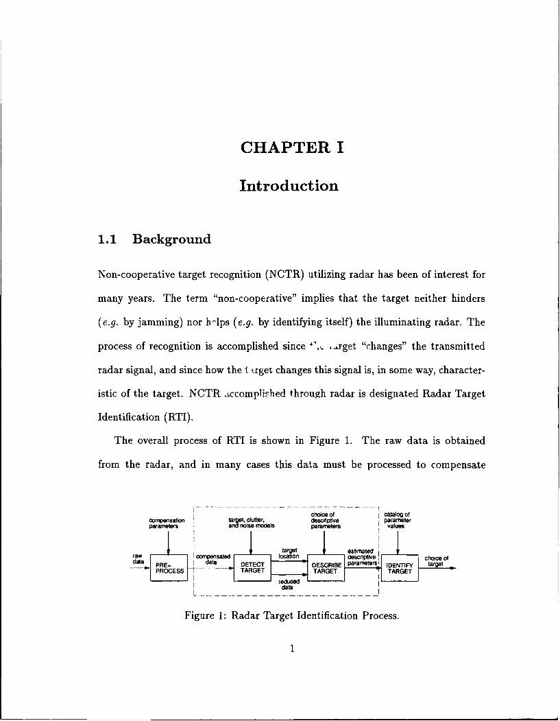
1 Radar Target Identification Process ......................... 1
2 Radar Target orientation ............................... 18
3 Standard spherical coordinate system ....................... 24
4 Impulse response approximation for a conducting sphere, taken from [1]. 25
5 Frequency domain response for a conducting sphere, taken from [2] . 26
6 Definition of a corner and an edge ......................... 27
7 MM impulse response estimation for a 0.5m square inclined flat plate. 30
8 MM frequency response estimation for the leading edge of the plateshown in Figure 7 ................................... 31
9 GTD impulse response estimation for the leading edge of the plateshown in Figure 7 ................................... 33
10 GTD frequency response estimation for the leading right corner ofthe plate shown in Figure 7 ............................. 35
11 MM frequency response estimation for the leading right corner of theplate shown in Figure 7 ................................ 36
12 GTD azimuthal angular response estimation for the leading left cornerof a 0.5m flat plate ................................... 37
13 GTD elevation angular response estimation for the leading left cornerof a 0.5m flat plate ................................... 38
ix
14 GTD azimuthal angular response estimation for the leading edge ofa 0.5m flat plate .................................... 39
15 Sketch of a typical dihedral ............................. 40
16 GTD frequency and time domain response estimates for the scatteringfrom a rectangular dihedral taken from [3] .................... 41
17 MM time domain response estimate for the scattering from a dihedral. 42
18 MM frequency response estimate for the scattering from a dihedral. 43
19 MM angular response estimate for the scattering from a dihedral. . 44
20 Definition of a trihedral ................................ 46
21 MM frequency domain response estimate for the scattering from atrihedral .......................................... 47
22 MM angular response estimate for the scattering from a trihedral. . . 48
23 Broadside angle of incidence off of a flat plate ................. 49
24 GTD frequency domain response estimate for the scattering from aflat plate .........................................
25 Sketch of a right circular cylinder .......................... 52
26 Damped exponential modeling for frequency dependencies of scatter-ing centers with types t = -1 and t = -0.5 ................... 59
27 Damped exponential modeling for frequency dependencies of scatter-ing centers with types t = 0 and t = 0.5 ..................... 60
28 Damped exponential modeling for frequency dependence of scatteringcenter with type t = 1 ................................. 61
29 Damped exponential modeling for scattering center angular depen-dencies of a constant and U(V)) ........................... 64
30 Damped exponential modeling for scattering center angular depen-dence of b(V) ....................................... 65
31 Impulse response estimation for an inclined flat plate from ESL data. 71
x
32 Impulse response estimation for an inclined flat plate from ESL data. 72
33 Impulse response estimation for an inclined flat plate from ESL datafor limited bandwidth ................................. 76
34 Impulse response estimation for an inclined flat plate from ESL datafor limited bandwidth using SVD-Prony method ............... 77
35 Radar-target geometry for 2-D imaging .................... 78
36 2-D frequency domain data set for full angular coverage .......... 81
37 2-D frequency domain data set for limited angular coverage ...... .82
38 Image of a plate, in the flat plate orientation, generated by directnumerical integration of Equation 4.24 for full angular coverage data(hh-polarization) .................................... 84
39 Image of a plate (inclined plate orientation) generated by direct nu-merical integration of Equation 4.24 for full angular coverage data(hh-polarization) .................................... 86
40 Desired point on rectangular grid between data points on polar grid.. 87
41 Image of a flat plate generated by interpolation to a square grid fol-
lowed by the 2-D IFFT for full angular coverage data (hh-polarization). 88
42 Image of an inclined plate generated by interpolation to a squaregrid followed by the 2-D IFFT for full angular coverage data (hh-
polarization) ....... ................................ 89
43 Image of an inclined plate generated for limitc! angular coverage data(hh-polarization) for off corner incidence ..................... 90
44 Image of an inclined plate generated for limited angular coveiage data(hh-polarization) for off edge incidence ....................... 92
45 2-D frequency locations for Example 1 ...................... 115
46 Example 1. 10log10 (1/Variance) versus total SNR in dB for x-pole
and y-pole frequencies using Algorithm One .................. 116
xi
47 Example 1. 101ogl 0 (1/Variance) versus total SNR in dB for x-pole
and y-pole magnitudes using Algorithm One ................. 118
48 Example 1. 10logl 0 (1/Variance) versus total SNR in dB for x-poleand y-pole frequencies using Algorithm Two ................. 120
49 Example 1. 101ogl 0 (1/Variance) versus total SNR in dB for x-pole
and y-pole magnitudes using Algorithm Two ................. 121
50 Example 2. 101ogl 0 (1/Variance) versus total SNR in dB for x-pole
and y-pole frequencies using Algorithm Two ................. 123
51 Example 2. 101ogl0 (1/Variance) versus total SNR in dB for x-pole
and y-pole magnitudes using Algorithm Two ................. 124
52 Polarization ellipse of scattering center consistent with IEEE standard. 129
53 Polarization ellipse of scattering center as viewed traveling toward the
radar (observer). All of the ellipses plotted in this dissertation followthis convention ..................................... 130
54 Polarization ellipses for Example FP1 ....................... 141
55 Example FP1. 101ogl 0 (1/Variance) versus total SNR in dB for x-poleand y-pole frequencies using FPA2 ......................... 142
56 Example FP1. 101ogl0 (1/Variance) versus total SNR in dB for x-poleand y-pole magnitudes using FPA2 ......................... 143
57 Example FP2. 101ogl0 (1/Variance) versus total SNR in dB for x-pole
and y-pole frequencies using Algorithm FPA2 ................. 145
58 Example FP2. 10log10 (1/Variance) versus total SNR in dB for x-poleand y-pole magnitudes using Algorithm Two ................. 146
59 Thin metal perfectly conducting square plate analyzed ......... .148
60 Geometry for scattering measurements from plate .............. 154
61 2-D frequency plane plot of scattering data collected by radar..... .155
62 Contour image of plate for 0 = 450 generated from a 150 polar swathof hh-polarization data ................................ 156
xii
63 Single polarization inclined plate example for a a 150 swath of polardata centered around 00. Model orders were Q, K, R, L = 10,2,10,2. . 159
64 Single polarization inclined plate example for a 150 swath of polardata centered around 00 and 7.5' . Model orders were Q, K, R, L =
10,2,10,2 for 0' and Q, K, R, L = 10,4,10,2 for 7.50 ........... 160
65 Single polarization inclined plate example for a 150 swath of polardata centered around 7.5' . Model orders were Q, K, R, L = 10,4,10,2. 161
66 Single polarization inclined plate example for a 150 swath of polardata centered around 150. Model orders were Q, K, R, L = 10,4,10,1. 162
67 Single polarization inclined plate example for a 150 swath of polar
data centered around 150 and 300. Model orders were Q, K, R, L =10,4,10,1 for 150 and 30 .......... ........................ .163
68 Single polarization inclined plate example for a 150 swath of polardata centered around 30'. Model orders were Q, K, R, L = 10,4,10,1. 164
69 Single polarization inclined plate example for a 150 swath of polardata centered around 450. Model orders were Q, K, R, L = 10,4,10,1. 165
70 Single polarization inclined plate example for a 150 swath of polardata centered around 450 and 600. Model orders were Q, K, R, L =
10,4,10,1 for 450 and 60 .......... ........................ .166
71 Single polarization inclined plate example for a 150 swath of polardata centered around 600. Model orders were Q, K, R, L = 10,4,10,1. 167
72 Single polarization inclined plate example for a 150 swath of polardata centered around 75' . Model orders were Q, K, R, L = 10,4,10,1. 168
73 Single polarization inclined plate example for a 150 swath of polardata centered around 750 and 82.50. Model orders were Q, K, R, L =10,4,10,1 for 750 and Q, K, R, L = 10,4,10,2 for 82.5 ............. .. 169
74 Single polarization inclined plate example for a 150 swath of polardata centered around 82.50. Model orders were Q, K, R, L = 10,4,10,2.170
75 Single polarization inclined plate example for a 150 swath of polardata centered around 900. Model orders were Q, K, R, L = 10,2,10,2. 171
xiii

76 Single polarization inclined plate example for a 150 swath of polar
data centered around 90'. Model orders were Q, K, R, L = 10,2,10,2.The polarization is vv ................................. 172
77 RE versus SNR for noise added to the GTD data of the plate. Allthree polarizations are shown for 0 = 00 and 40 = 45' . The model
orders were Q, K, R, L = 10,2,10,2 for the 0 = 00 plots and Q, K, R, L
= 10,4,10,1 for the 4 = 450 plots. The data is a 150 swath of polardata ............................................ 175
78 Single polarization inclined plate example for a 15' swath of polardata centered around 00. Model orders were Q, K, R, L = 10,4,10,4. 177
79 Single polarization inclined plate example for a 15' swath of polardata centered around 7.5' . Model orders were Q, K, R, L = 10,6,10,4. 178
80 Single polarization inclined plate example for a 150 swath of polardata centered around 15'. Model orders were Q, K, R, L = 10,6,10,4. 179
81 Single polarization inclined plate example for a 150 swath of polar
data centered around 300. Model orders were Q, K, R, L = 10,6,10,4. 180
82 Single polarization inclined plate example for a 150 swath of polardata centered around 450. Model orders were Q, K, R, L = 10,6,10,4. 181
83 Single polarization inclined plate example for a 150 swath of polardata centered around 600. Model orders were Q, K, R, L = 10,6,10,4. 182
84 Single polarization inclined plate example for a 150 swath of polardata centered around 75' . Model orders were Q, K, R, L = 10,6,10,4. 183
85 Single polarization inclined plate example for a 15° swath of polardata centered around 82.50. Model orders were Q, K, R, L = 10,6,10,4.184
86 Single polarization inclined plate example for a 150 swath of polardata centered around 90' . Model orders were Q, K, R, L = 10,4,10,4. 185
87 RE versus SNR for noise added to the GTD data of the plate. Allthree polarizations are shown for 4' = 00 and 4, = 450. The model
orders were Q, K, R, L = 10,4,10,4 for the 4, = 00 plots and Q, K, R, L
= 10,6,10,4 for the 4, = 450 plots. The data is a 150 swath of polar
data ............................................ 188
xiv
88 Single polarization inclined plate example for a square grid (from 150polar) of data centered around 0'. Model orders were Q, K, R, L =10,2,10,2 ....... .................................. 191
89 Single polarization inclined plate example for a square grid (from15' polar) of data centered around 0' and 7.5' . Model orders wereQ, K, R, L = 10,2,10,2 for 00 and Q, K, R, L = 10,4,10,2 for 7.5. .... 192
90 Single polarization inclined plate example for a square grid (from 150polar) of data centered around 7.5' . Model orders were Q, K, R, L =10,4,10,2 ....... .................................. 193
91 Single polarization inclined plate example for a square grid (from 150polar) of data centered around 15'. Model orders were Q, K, R, L =10,4,10,1 ....... .................................. 194
92 Single polarization inclined plate example for a square grid (from
15' polar) of data centered around 150 and 30'. Model orders were
Q, K, R, L = 10,4,10,1 for 150 and 30 ....... ................ .. 195
93 Single polarization inclined plate example for a square grid (from 150
polar) of data centered around 30' . Model orders were Q, K, R, L =10,4,10,1 ....... .................................. 196
94 Single polarization inclined plate example for a square grid (from 150polar) of data centered around 45' . Model orders were Q, K, R, L =10,4,10,1 ....... .................................. 197
95 Single polarization inclined plate example for a square grid (from
150 polar) of data centered around 450 and 600. Model orders wereQ, K, R, L = 10,4,10,1 for 450 and 60 ....... ................ .. 198
96 Single polarization inclined plate example for a square grid (from 150polar) of data centered around 600. Model orders were Q, K, R, L =10,4,10,1 ....... .................................. 199
97 Single polarization inclined plate example for a square grid (from 150polar) of data centered around 75' . Model orders were Q, K, R, L =10,4,10,1 ....... .................................. 200
xv

98 Single polarization inclined plate example for a square grid (from 150polar) of data centered around 750 and 82.50. Model orders wereQ, K, R, L = 10,4,10,1 for 750 and Q, K, R, L = 10,4,10,2 for 82.50. . 201
99 Single polarization inclined plate example for a square grid (from 150
polar) of data centered around 82.5'. Model orders were Q, K, R, L= 10,4,10,2 ....................................... 202
100 Single polarization inclined plate example for a square grid (from 150polar) of data centered around 90'. Model orders were Q, K, R, L =10,2,10,2 ....... .................................. 203
101 Single polarization inclined plate example for a square grid (from 150polar) of data centered around 900. Model orders were Q, K, R, L =10,2,10,2. The polarization is vv ......................... 204
102 RE versus SNR for noise added to the GTD data of the plate. Allthree polarizations are shown for 0 = 00 and 4, = 450. The modelorders were Q, K, R, L = 10,2,10,2 for the 4, = 00 plots and Q, K, R, L= 10,4,10,1 for the 4, = 450 plots. The data lies on a square gridinterpolated from a 150 swath of polar data .................. 206
103 Single polarization inclined plate example for a 30 polar swath of datacentered around 00. Model orders were Q, K, R, L = 10,2,10,2 ..... .209
104 Single polarization inclined plate example for a 30 polar swath ofdata centered around 00 and 7.5' . Model orders were Q, K, R, L =10,2,10,2 for 00 and Q, K, R, L = 10,4,10,2 for 7.50 ........... 210
105 Single polarization inclined plate example for a 30 polar swath of datacentered around 7.5' . Model orders were Q, K, R, L = 10,4,10,2. . . . 211
106 Single polarization inclined plate example for a 30 polar swath of datacentered around 15'. Model orders were Q, K, R, L = 10,4,10,1. . . . 212
107 Single polarization inclined plate example for a 30 polar swath ofdata centered around 15' and 300. Model orders were Q, K, R, L =10,4,10,1 for 150 and 30 ................................ 213
108 Single polarization inclined plate example for a 30 polar swath of datacentered around 30' . Model orders were Q, K, R, L = 10,4,10,1 .... 214
xvi
109 Single polarization inclined plate example for a 30 polar swath of datacentered around 450. Model orders were Q, K, R, L = 10,4,10,1. . . . 215
110 Single polarization inclined plate example for a 30 polar swath ofdata centered around 45' and 600. Model orders were Q, K, R, L =10,4,10,1 for 450 and 60 .......... ........................ .216
III Single polarization inclined plate example for a 30 polar swath of datacentered around 600. Model orders were Q, K, R, L = 10,4,10,1. . . . 217
112 Single polarization inclined plate example for a 30 polar swath of datacentered around 75'. Model orders were Q, K, R, L = 10,4,10,1. . . . 218
113 Single polarization inclined plate example for a 30 polar swath ofdata centered around 750 and 82.50. Model orders were Q, K, R, L -
10,4,10,1 for 750 and Q, K, R, L = 10,4,10,2 for 82.5 .......... .219
114 Single polarization inclined plate example for a 30 polar swath of datacentered around 82.5'. Model orders were Q, K, R, L = 10,4,10,2. . . 220
115 Single polarization inclined plate example for a 30 polar swath of datacentered around 900. Model orders were Q, K, R, L = 10,2,10,2. . . . 221
116 Single polarization inclined plate example for a 30 polar swath of datacentered around 900. Model orders were Q, K, R, L = 10,2,10,2. Thepolarization is vv .................................... 222
117 RE versus SNR for noise added to the GTD data of the plate. Allthree polarizations are shown for 0 = 0' and 0 = 45' . The modelorders were Q, K, R, L = 10,2,10,2 for the 4k = 00 plots and Q, K, R, L= 10,4,10,1 for the 0 = 450 plots. The data is a 30 swath of polar data.223
118 RE versus SNR for noise added to the GTD data of the plate. Allthree polarizations are shown for 4 = 300. The model orders areQ, K, R, L = 10,4,10,1. The data is a 30 swath of polar data ...... .224
119 Estimated pole locations for noise corrupted GTD data. The GTDdata is a 30 polar swath with hh-polarization centered around 4 = 45' .
The model orders were Q, K, R, L = 10,4,10,1 ................ 227
xvii
120 Estimated pole locations for noise corrupted GTD data. The GTDdata is a 30 polar swath with hh-polarization centered around 0 = 450 .
The model orders were Q, K, R, L = 10,4,10,2 ................ 228
121 Full polarization flat plate example for a 15' polar swath of datacentered around 0', 7.50, 150 and 300 ............... 232
122 Full polarization flat plate example for a 150 polar swath of datacentered around 450, 60', 750 and 82.5 ....... ............... .233
123 Full polarization flat plate example for a 150 polar swath of datacentered around 90 .......................... 234
124 RE versus SNR for noise added to the GTD data of the plate. Fullpolarization results are shown for q0 = 00 and 0 = 45' . The model
orders were Q, K, R, L = 10,2,10,2 for the 0 = 00 plot and Q, K, R, L= 10,4,10,1 for the 0 = 45' plot. The data is a 150 swath of polar data.235
125 Full polarization flat plate example for a 150 polar swath of datacentered around 00, 7.50, 150 and 300 with higher model orders chosen.238
126 Full polarization flat plate example for a 15' polar swath of datacentered around 450, 600, 750 and 82.50 with higher model orderschosen ........................................... 239
127 Full polarization flat plate example for a 150 polar swath of datacentered around 90' with higher model orders chosen ........... 240
128 RE versus SNR for noise added to the GTD data of the plate. Fullpolarization results are shown for 0 = 00 and 0 = 450. The modelorders were Q, K, R, L = 10,4,10,4 for the 4 = 00 plot and Q, K, R, L= 10,6,10,4 for the 40 = 450 plot. The data is a 150 swath of polar data. 241
129 Full polarization flat plate example for a square grid of data inter-polated from a 150 polar swath of data centered around 00, 7.50, 150and 300 ............ ................................... .242
130 Full polarization flat plate example for a square grid of data interpo-lated from a 150 polar swath of data centered around 450, 600, 750and 82.5 .............. ................................ .243
xviii

131 Full polarization flat plate example for a square grid of data interpo-lated from a 150 polar swath of data centered around 900 ........... 245
132 RE versus SNR for noise added to the GTD data of the plate. Full
polarization results are shown for 0 = 00 and q = 450. The modelorders were Q, K, R, L = 10,2,10,2 for the 0 = 0' plot and Q, K, R, L= 10,4,10,1 for the q = 450 plot. The data lies on a square grid whichwas interpolated from a 15' swath of polar data ............... 247
133 Full polarization flat plate example for a 30 polar swath of data cen-tered around 00, 7.5', 150 and 300 .................. 248
134 Full polarization flat plate example for a 30 polar swath of data cen-tered around 450, 600, 750 and 82.5 ........ ................. .249
135 Full polarization flat plate example for a 30 polar swath of data cen-tered around 900 .......... .............................. .250
136 RE versus SNR for noise added to the GTD data of the plate. Full
polarization results are shown for 0 = 00, 4 = 300, and 0 = 450 .
The model orders were Q, K, R, L = 10,2,10,2 for the 0 = 00 plot andQ, K, R, L = 10,4,10,1 for the ¢ = 300 and € = 450 plots. The data
is a 30 swath of polar data .............................. 251
137 Estimated ellipses for noise corrupted GTD data. The GTD data isa full-polarization 30 polar swath. The model orders were Q, K, R, L
= 10,4,10,1 for all of the plots ............................ 252
138 Estimated ellipses for noise corrupted GTD data. The GTD data isa full-polarization 30 polar swath. The model orders were Q, K, R, L
= 10,4,10,2 for all of the plots ............................ 253
139 Frequency response comparisons for parameter estimates from a squaregrid of data generated from a 150 polar swath of data centered around
€ = 450 .............. ................................... 258
140 Angular response comparisons for parameter estimates from a squaregrid of data generated from a 150 polar swath of data centered around0 = 450 ................................. 259
141 Frequency response comparisons for parameter estimates from a 30polar swath of data centered around € = 45 ............. 260
xix

142 Angular response comparisons for parameter estimates from a 30 polarswath of data centered around 0 = 450 ............... 261
xx

LIST OF TABLES
TABLE PAGE
1 Approximate Frequency and Angle characteristics of canonical scat-tering centers ....................................... 53
2 Correspondence between terms in damped exponential scattering modeland electromagnetically based scattering model ................ 57
3 Summary of amplitude coefficients and poles for 1-D frequency do-main scattering from canonical scattering centers ............... 62
4 Summary of amplitude coefficients and poles for 1-D angular domainscattering from canonical scattering centers ................... 63
5 Summary of steps performed in Algorithm One ............... 106
6 Summary of steps performed in Algorithm Two ............... 109
7 Summary of steps performed in FPA1 ....................... 137
8 Summary of steps performed in FPA2 ...................... 139
9 Model orders and relative errors for single polarization results for thescattering from an inclined plate. The data is a 15' polar swath. . . . 158
10 Model orders and relative errors for single polarization results for thescattering from an inclined plate with model orders larger than theirodel orders in Table 9. The data is a 150 polar swath ......... .187
11 Model orders and relative errors for single polarization results for thescattering from an inclined plate. The data lies on a square grid (from15' polar swath) .................................... 205
12 Model orders and relative errors for single polarization results for thescattering from an inclined plate. The data is a 30 polar swath .... 225
xxi

13 Model orders and relative errors for full-polarization results for thescattering from an inclined plate. The data is a 150 angular swath ofpolar data ........................................ 236
14 Model orders and relative errors for full-polarization results for thescattering from an inclined plate. The model orders for these exam-ples were chosen higher than the model orders in Table 13. The datais a 15' angular swath of polar data ....................... 244
15 Model orders and relative errors for full-polarization results for thescattering from an incintd plate. The data lies on a square grid andwas interpolated from a 150 polar swath of data ............... 246
16 Model orders and relative errors for full-polarization results for thescattering from an inclined plate. The data is a 30 angular swath ofpolar data ........................................ 254
xxii

ABSTRACT
This dissertation develops one and two-dimensional signal processing models and
algorithms which are utilized in the Radar Target Identification Problem. A basic
assumption of this work is that the high-frequency scattering from a radar target,
such as an aircraft, land-based vehicle, or ship, is comprised of the sum of the
scattering from a finite number of canonical scattering centers, each with a specific
location and identity. By high-frequency it is meant that the overall size of the
target is at least one wavelength. The scattering center assumption is more valid as
the individual scattering centers become more electrically isolated. If two individual
scattering centers are electrically close, then their combined response is, in general,
not the sum of their individual responses.
First, this dissertation investigates the electromagnetic scattering characteristics
of canonical scattering centers. Canonical scattering centers are scattering centers
on a target which account for the vast majority of the scattering from that target
in the high-frequency case. Some of the targets of interest in this work are aircraft,
tanks, trucks, automobiles and ships. Predominant scattering centers on these tar-
gets include corners, edges, plates, dihedrals, trihedrals, and cylinders. The scat-
tering centers are described by their scattering characteristics as functions of angle,
frequency, and polarization.
xXii

Second, this dissertation develops a two-dimen.ional (2-D) signal processing tech-
nique for locating and characterizing scattering centers from radar data. The radar
gathers scattering data of a target at both multiple frequencies and multiple angles.
This type of data is gathered (in raw form) by both Synthetic Aperture Radars and
Inverse Synthetic Aperture Radars. The 2-D signal processing technique developed
here is based on a a 2-D extension of a total least squares (TLS) solution to a Prony
Model and is called the 2-D TLS-Prony Technique. This technique can use single or
multiple-polarization data. With full-polarization data, polarimetric characteristics
of the scattering centeis are found using the transient polarization response concept.
This concept uses an ellipse to characterize the polarimetric characteristics of each
scattering center. The abilities of the 2-D TLS-Prony Technique are demonstrated
utilizing simulated 2-D radar data.
xxiv
CHAPTER I
Introduction
1.1 Background
Non-cooperative target recognition (NCTR) utilizing radar has been of interest for
many years. The term "non-cooperative" implies that the target neither hinders
(e.g. by jamming) nor blps (e.g. by identifying itself) the illuminating radar. The
process of recognition is accomplished since 4', ,rget "changes" the transmitted
radar signal, and since how the i Srget changes this signal is, in some way, character-
istic of the target. NCTR Lccomplished through radar is designated Radar Target
Identification (RTI).
The overall process of RTI is shown in Figure 1. The raw data is obtained
from the radar, and in many cases this data must be processed to compensate
choice of catalog ofcompensation I target, clutter, descriptive parameterparameters and noise models parameters values
raw mpensated oation scriptive, choice ofdata- PRtE- Idata DETECT DESCRIBE Parameters' IDE"~FY tare
POESTARGET TARGET ITARGET
dataL ----.--------- _------- - -
Figure 1: Radar Target Identification Process.

2
for factors such as radar target velocity, radar target orientation, radar antenna
characteristics, path of radar relative to target and radar target range. Once the
data has been preprocessed, it is ready to be used by the target detection algorithm.
The purpose of the target detection algorithm is to detect the presence of and
estimate the location of a target. Also, this algorithm may reduce the data set to
yield another smaller data set that still contains the important target descriptive
information. The target location and the reduced data set are passed onto the target
description algorithm. This algorithm takes the target location and the reduced data
set and forms an estimated descriptive parameter set which describes the target of
interest. This descriptive parameter set is sent to a target identification algorithm
and compared with idealized parameter sets, and a classification of the target is
made.
1.2 Description of Study
This dissertation focuses on and develops one-dimensional (1-D) and two-dimensional
(2-D) signal processing models and algorithms which are utilized in the target de-
tection and target description stages of the RTI process. A basic assumption of
this work is that the high-frequency scattering from a complicated target such as
an aircraft, land-based vehicle, or tank is comprised as the sum of the scattering
from a finite number of canonical scattering centers, each with a specific location
and identity (e.g. corner, edge, dihedral, etc.). This assumption is more valid as
the individual scattering centers become more electrically isolated (electrical iso-
lation between two scattering centers implies that the physical distance between

3
the two scattering centers is several or more wavelengths, where the wavelength
is the wavelength of the electromagnetic wave illuminated by the radar). If two
individual scattering centers are electrically close (physically, less than or around
one wavelength apart), then their combined response is, in general, not the simple
sum of their individual responses. Also, if the overall target size is less than one
wavelength, then the phenomena of resonance will dominate the scattering from
the object, and the scattering center assumption fails. Thus, the scattering center
assumption is considered high-frequency, which implies that the size of the overall
target is a wavelength or greater.
First, this dissertation investigates the electromagnetic characteristics of canoni-
cal scattering centers. Canonical scattering centers are scattering centers on a target
which account for the vast majority of the scattering from that target in the high-
frequency case. Some of the targets of interest in this work are aircraft, tanks,
trucks, automobiles, and ships. Predominant scattering centers on these targets
include corners, edges, plates, dihedrals, trihedrals, and cylinders. The scattering
centers are described by their scattering characteristics as functions of angle, fre-
quency, and polarization. The scattering centers in this work are assumed to be
perfect conductors.
Second, this dissertation develops a 2-D signal processing technique for locating
and characterizing scattering centers from radar data. By 2-D, it is meant that the
radar gathers data on a target at multiple frequencies and multiple angles. It is
assumed that both the magnitude and phase of the received signal are known. This
4
type of data is gathered (in raw form) by both Synthetic Aperture Radars (SARs)
and Inverse Synthetic Aperture Radars (ISARs). The 2-D signal processing tech-
nique developed here is based on a a 2-D extension of a total least squares (TLS) so-
lution to a Prony Model and is called the 2-D TLS-Prony Technique. This technique
can use single or multiple-polarization data. With full-polarization data, polarimet-
ric characteristics of the scattering centers are found using the transient polarization
response (TPR) concept [4]. This concept uses an ellipse to characterize the polari-
metric characteristics of each scattering center.
1.3 Previous Work in Radar Target Identification
The techniques developed in this dissertation are useful for determining the identity
of a target from its structure. The determination of the physical characteristics
of a target from the scattering behavior of that target is, in general, an inverse
scattering problem. The general problem of inverse scattering is ill-posed [5]. Thus,
some assumptions must be made in order to make the RTI problem solvable.
The idea of approximating the impulse response of a target was described by
Kennaugh and Cosgriff in 1958 [6] and later by Kennaugh and Moffatt in 1965 [1].
Kennaugh and Moffatt also looked at other transient responses such as step responses
and ramp responses. In 1981, techniques were developed by Moffatt and others [7] to
utilize the impulse and other transient responses for target identification purposes.
These techniques all used the range (or time) domain responses which exploited the
geometrical characteristics of the targets. All of these techniques assumed a single
polarization and a single radar-target orientation.
5
Assuming that the scattering from a complicated target is made up of the sum of
the scattering from a finite number of scattering centers, the first step in analyzing
the scattering data from a target is to determine the presence and location of the
canonical scattering centers. Fourier techniques have been used successfully [4] by
taking the local maxima of the range domain waveform. Parametric techniques [8, 9]
have been used to determine the locations of the scattering centers for the 1-D
problem. The parametric techniques have been shown to have superior resolution
capabilities than the Fourier techniques [10]. A 1-D canonical scattering center
algorithm was developed by Carri6re and Moses [11]. This algorithm takes 1-D data
and returns the types (e.g. corner, edge), locations, and amplitudes of the canonical
scattering centers which comprise the target at that aspect angle.
This dissertation develops a new method for estimating 2-D frequencies and
amplitude coefficients from a 2-D data set. This method is applied to radar data in
this dissertation, but it can also be applied in other areas such as sonar, geophysics,
radio astronomy, radio communications, and medical imaging. The estimation of
2-D frequencies and amplitude coefficients from a 2-D data set has been investigated
utilizing many different approaches [12]-[181 such as Fourier-based methods, data
extension, maximum likelihood method (MLM), maximum entropy method (MEM),
autoregressive (AR) models, and linear prediction (LP) models [19]-[25].
Fourier-based methods are currently used in tomography to generate an image of
an object [131-[17]. The properties of these techniques have been well studied [13].
However, these techniques are limited by Fourier resolution capabilities. Also, these
6
techniques do not directly estimate 2-D frequencies. Thresholding along with a peak
detection scheme must be used in the 2-D frequency domain to determine the 2-D
frequencies.
Other methods include the MLM of spectral estimation which was proposed as
an m-dimensional (m-D) technique for array processing [19]. This technique has also
been applied to the tomography problem in [24]. The MEM of spectral estimation
has also been applied to the 2-D problem [21, 22, 25]. This method also provides high
resolution, but does not exist for all data sets [26]. Two-dimensional AR modeling
and algorithms exist [10, 20, 23], but these are computationally expensive. State
space methods [27] and a matrix pencil method [28] have also been used. Prony's
method coupled with total least squares (TLS) techniques in one-dimension (1-D)
has been used successfully to estimate frequencies in the presence of noise [29]. This
dissertation extends Prony's model to 2-D.
A related method 2-D method, developed by Hua [28], also estimates 2-D fre-
quencies. In Hua's method, two estimation steps are performed to separately esti-
mate the x-components and y-components of the 2-D frequencies. Then, a matching
step is performed to find the correct x-component and y-component frequency pair-
ings. The matrix pencil method is employed for noise cleaning purposes in Hua's
method.
The polarimetric characteristics of radar targets have been investigated for many
years. In the late 1940's and early 1950's Kennaugh [30] developed the concept
of an 'optimal polarization' for a target. This optimal polarization is found by
7
determining the eigenvalues of the monostatic, monochromatic scattering matrix.
The eigenvector corresponding to the largest eigenvalue yields the transmit and
receive polarization which yields the maximum received power of any polarization.
Also related to this is the 'null polarization' concept, which is the transmit and
receive polarization which provides zero received power.
Huynen developed a phenomenological theory of radar targets in [31] which ex-
tended the work of Kennaugh. Huynen characterized a target by a 3x3 set of
parameters based upon power quantities. This set of parameters closely resembles
the 4 x4 Stokes reflection matrix [32]. The Huynen parameters relate to the physi-
cal characteristics of the target. The Huynen approach is monochromatic. Boerner
used Kennaugh's optimal polarization concept and Huynen's work to analyze the
wideband scattering of radar targets [33]. The polarimetric properties of scattering
centers on the target are isolated by gating the response of the scattering center of
interest in the time domain. The Huynen parameters of the a scattering center on
the object are calculated for the center frequency of the wideband data. This work
confirmed the assumption that the high-frequency scattering from a complicated
radar target consists of the sum of the scattering from a finite number of scattering
centers.
Another polarimetric-based method, developed by Cameroon [34], used the po-
larimetric behavior of several canonical shapes. The scattering matrix for each scat-
tering center is decomposed into parts corresponding to non-reciprocal, asymmetric,
and symmetric scatterers. The decomposition proceeds further into specific scatter-
8
ing types which fit into one of the above three classes. Classification is accomplished
by determining the specific identity of each scattering center.
Chamberlin [4] introduced the transient polarization response concept (TPR).
In the TPR concept, the target is illuminated with an impulse of a circularly po-
larized electromagnetic wave and as the wave interacts with each scattering center
on the target, each scattering center will reflect back a wave with a polarization
which is determined by the polarimetric characteristics of that scattering center.
This concept has been investigated in 1-D utilizing nonparametric [4, 35, 36] and
parametric [37, 38] techniques. This dissertation extends the parametric-based TPR
method of Steedly [37, 38] to the 2-D case.
Classification work has been done utilizing the scattering center approach. Sands
in [391 used a data base of known targets and compared a candidate target to the
known targets. In this work, each target is described by a set of scattering centers;
only the scattering center location is important, and its identity is not used. The
data-base target that has the best "match" to the candidate target is declared the
winner. Other classification work, using statistical techniques such as the nearest
neighbor method, is reported in [40].
Much of the above work assumes that the scattering centers are of the point
scatterer variety; that is, the models only allow for undamped exponentials in one
or two-dimensions. This dissertation allows for 2-D damped exponentials. This is
important in modeling scattering centers which are not point scatterers, and thus
do not have scattering characteristics that are constant as a function of frequency
9
or angle.
1.4 Summary of Chapters
Chapter II defines the scattering matrix and how the scattering data is collected.
This is a background chapter which outlines the assumptions concerning the form
and content of the scattering matrix and how the scattering coefficients are related to
the radar data. Also, the conversion of the scattering matrix from one polarization
basis to another is outlined.
Chapter III investigates the scattering characteristics of canonical scattering cen-
ters. Techniques such as The Method of Moments (MM) and The Geometrical
Theory of Diffraction (GTD) are used to determine the scattering characteristics of
structures such as the edge, corner, dihedral, trihedraJ and cylinder. The scatter-
ing characteristics of each canonical shape are estimated as a function of frequency,
radar-target orientation, and polarization. The high-frequency scattering model for
a complicated radar target is defined, which is the sum of the scattering responses
from a finite number of canonical scattering centers. Finally, the ability of a damped
exponential model to accurately model the scattering characteristics of the canonical
scattering centers is discussed.
Chapter IV is a background signal processing chapter which is needed to intro-
duce 1-D and 2-D signal processing techniques. Non-parametric techniques such
as the 1-D and 2-D IFFTs are introduced and examples are shown on how these
techniques produce a down-range profile and an image of a target, respectively. The
l-D TLS-Prony Technique is described, which is a 1-D parametric signal processing
10
technique. Prony's model (in 1-D) is introduced, which is the 1-D damped exponen-
tial model used by the 1-D TLS-Prony Technique. The estimation algorithm used
by this technique is described, and examples are shown which illustrate this 1-D
technique. Several 2-D IFFT based image generation techniques are also described.
Images generated by the various techniques are also shown.
Chapter V develops the 2-D TLS-Prony Technique. This is a new technique for
estimating two-dimensional (2-D) poles and amplitude coefficients in a 2-D Prony-
based model. The fundamental estimation algorithm involves two parts, each uti-
lizing a 1-D singular value decomposition-based technique. This 2-D technique is
capable of locating frequencies anywhere in the 2-D frequency plane. The basic
algorithm is first developed for a single 2-D data set, such as a set of radar mea-
surements with a single transmit and receive polarization. Simulations are shown
which demonstrate the performance of the algorithm for various noise levels. Then,
the algorithm is extended to the multiple data set case, which applies when full-
polarization 2-D measurements of a target are available. Simulations are shown
which demonstrate the performance of this algorithm for the multiple data set case
for various noise levels.
Chapter VI discusses examples of the 2-D TLS-Prony Technique applied to sim-
ulated radar data. The scattering from an inclined thin metal plate is generated
using the Geometrical Theory of Diffraction (GTD). This data is used by both the
single-polarization and the full-polarization 2-D TLS Prony Techniques to estimate
the locations and the polarimetric characteristics of the scattering centers on the

11
plate. Issues involving 2-D angular and frequency bandwidths, model order selec-
tion, effects of noise on parameter estimates, and the form of the data set on the
2-D frequency plane are addressed. Also, the validity of the damped exponential to
model the scattering from the canonical scattering centers is addressed.
Finally, Chapter VII provides a summary and draws conclusions based upon the
work presented in the dissertation. Also, areas for future research are discussed.
CHAPTER II
Target Scattering Fundamentals
2.1 Background and Introduction
This chapter describes how target-scattering information is acquired by a radar.
A target's scattering characteristics in the far field are contained in its scattering
matrix. The scattering matrix contains multiple polarization information for a given
object at a given orientation relative to the radar at a specific frequency. In its
most general form, the scattering matrix for a target is a function of frequency
of illumination, target orientation, and transmit and receive polarizations. It is
possible for a target to have both monostatic and bistatic scattering matrices. For
this research, only the monostatic case is investigated.
2.2 Electromagnetic Fundamentals
It is assumed that the target is in the far-field of the radar antenna. Thus, a locally
plane wave is assumed to impinge upon the target. A plane wave is the solution
to the homogeneous wave equation. Consider Maxwell's Equations in their time
domain point form:V x _(, 0 &
12
13
atVX W(R,t) = (Rt)
V.9=t) 0. (2.1)
The spatial position of the field quantities is denoted by R (R would be x, y, z for the
standard rectangular coordinate system) and t denotes time in Equation 2.1. Note
that the field quantities above are vectors. In this chapter, vectors are designated by
an arrow over the vector quantity (e.g. E) and complex numbers are designated by
boldface quantities (e.g. E). It is assumed that the media of propagation between
the radar and target is ideal free space, which is linear, time-invariant, homogeneous,
isotropic, dispersionless, and lossless. With the use of the Fourier Transform, to
convert from the (R,t) domain to the (R,w) domain, Maxwell's Equations can be
expressed in the frequency domain point form as
V x F,(R,w) = -jwI3(R,w)
V xH(R,w) = )+,)+jw](R, w)
V.D(R,w) = p,(R,w)
V.IB(?,w) = 0 (2.2)
where w denotes the radian frequency. It will be assumed that all of the above field
terms (in Equations 2.2) are time-harmonic [41], and thus contain an implicit ej "w
term. This term is suppressed for the remainder of this work. The constitutive
relations for free space are
=E oE (2.3)
7
14
f3 - /oI . (2.4)
It is well known that the field due to a point source of current is proportional to
e-jkor where r is the distance from the point source to the observation point andT
k=, where A,, is the wavelength of the electromagnetic wave in free space. This
is the mathematical representation for a spherically expanding wave. However, for
this research, it is assumed that the target is in the far field of the radar antenna.
Thus, it is assumed that the incident electromagnetic field is "locally-plane" around
the target. An expression for a plane wave is found by solving Maxwell's Equations
in a source-free region (source-free means that J, (R, w) - 0 and p,, (t) - 0). With
some manipulation of Equations 2.2-2.4 the free space wave-equation is found and
given by
V2t 2-koE = 0, (2.5)
where
ko = O = 21r (2.6)
VPE=A 0 .
A solution to this wave-equation is a plane wave and is given by
E (Rw) = E (R, w) f3, (2.7)
where
E (Kw) = Eeoei jko , (2.8)
and
E. = IE (R,w) . (2.9)

15
The absolute value signs take the magnitude of the complex scalar E (R, w). The
term f) is a complex unit vector which expresses the direction (or polarization) of
the electric field. The terms E, and 0,o are the arbitrary magnitude and phases of
the electric field, respectively. This wave is traveling in the positive r direction. The
term P has the properties
p .15" = 1, (2.10)
P5 P*L = * - 0, (2.11)
where * denotes complex conjugate. The unit vector 15z is defined to be orthogonal
to the unit vector 5. Using linear combinations of these vectors, it is possible to
construct any desired polarization.
2.3 Scattering Matrix Formulation
As stated before, the scattering matrix relates the transmitted electric field to the
scattered electric field. The transmitted electric field will be expressed as the lin-
ear combination of a horizontally polarized component and a vertically polarized
component. Thus,
Et= Ph + EtPv. (2.12)
The transmitted electric field is a function of range from the radar (or transmitter).
The electric field incident upon the target at a range ro from the radar is given by
D r = (r,). (2.13)
Of course, most targets have physical size and are not located at a single point. It
is assumed that the magnitude of the incident field is constant in the vicinity of the
16
target, but the phase of the incident field is not. The incident electric field at a
distance ri from the reference point r, is given by
E' (r,) = EAo2), (2.14)
where
Eo= IE'(r)I, (2.15)
and 0 is an arbitrary phase constant. The point ro on the target will be called the
phase reference point on the target.
The scattered electric field, D, is a function of range from the target (the refer-
ence point on the target, designated r, for the incident electric field, is considered
the origin for the scattered electric field). Thus, the incident electric field and the
scattered electric field can be expressed in the following matrix relationship as
E-) = ahh(w) ah (W) E,(w)(1 avh (w) a. (uw) j Ei (w)
where the incident field value is measured at the point r, and the scattered field is
measured back at the radar. Equation 2.16 shows how the polarization of the scat-
tered field may be different than the polarization of the incident field, and thus, the
target "changes" the polarization of the electromagnetic wave. Since the scattered
field is measured at the radar, and it is known that the scattered field will expand
spherically in the far field, the e- k° term, where r is the distance from the phase
reference point on the target to the radar, can be taken out of the scattering matrix.
This is a more convenient way to express the scattering matrix. The a coefficients

17
can be written as
axy = Sxy XY E [hh, hv, vh, vv]. (2.17)r
Using Equations 2.17 and 2.16, the incident and scattered electric fields are now
related by
=-' w Shh (W) Sh1, (W) ir E (w) 1 eio\ (2.18)1E! ,(w) = v s (w) s,, (w) jE"' P ) r)
where the four sxy elements form the scattering matrix. The scattering matrix
above is a function of frequency only (and not range). This is true as long as the
radar and target are fixed in space relative to one another. As the radar-target
orientation changes (in aspect angle), the scattering matrix changes. It is assumed
in this research that the range between the radar and the designated phase center
on the target remains fixed. If this is not the case, then corrections can be made
to the data to achieve this situation [421. Thus, the Sxy elements, denoted the
scattering coefficients, are a function of radar-target orientation. For the purposes
of the scattering matrix, only one set of angles, (0, €), is required to designate the
radar-target orientation.
In SAR, the radar moves while the target remains fixed, whereas in ISAR, the
radar remains fixed while the target moves. The scattering coefficients are identical
for either scenario. It is assumed that the scattering coefficients correspond to the
scenario where there is no relative velocity between the target and the radar. If this is
not the case, then the measurements can be corrected to simulate this situation [42].
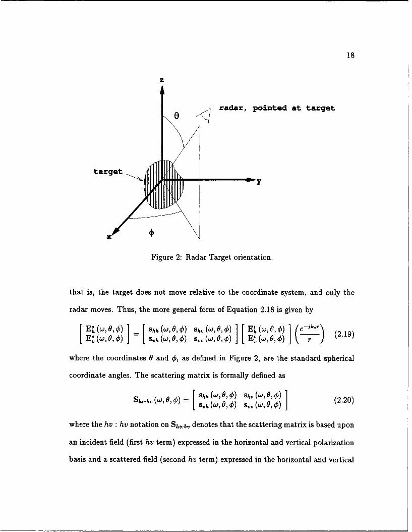
Figure 2 shows the radar-target orientation. This is a target fixed coordinate system;
18
Z
0 radar, pointed at target
target
Figure 2: Radar Target orientation.
that is, the target does not move relative to the coordinate system, and only the
radar moves. Thus, the more general form of Equation 2.18 is given by
E h (w, 0, €)Shh ( ,O, ) Sh, (W, , ¢) 1[E l (w, , e€)k~ (2.19)E'(w, 0,) =~ s(W, 0,¢ s,,(w, 0, ) E (w, 0,¢r
where the coordinates 0 and €, as defined in Figure 2, are the standard spherical
coordinate angles. The scattering matrix is formally defined as
Shv:hv (w, 0, ) = rShh (w, 0, 0) Shv (w, 0, ) 1 (2.20)
where the hv : hv notation on Sh,.h,, denotes that the scattering matrix is based upon
an incident field (first hv term) expressed in the horizontal and vertical polarization
basis and a scattered field (second hv term) expressed in the horizontal and vertical
19
polarization basis.
The radar cross section (RCS) of an object can be determined from the scattering
coefficients. The RCS of an object is defined as
axy(w,o,;) =lim (4rr 2IE (w, 0, 0, r) 12 (2.21)r~oo ( Ei(w, 0,0, r) 12
Comparing Equations 2.19 and 2.21, it is observed that
xy = 41rlsxY 2. (2.22)
The choice of a horizontal and vertical polarization basis was arbitrary and any
two linearly independent bases could be chosen [31]. Usually, orthogonal bases such
as left circular-right circular or horizontal-vertical are used. The scattering matrix
will change when different polarization bases are chosen. However, the scattering
matrix contains all of the inherent target information.
The conversion of the scattering matrix from one polarization basis to another
is easily accomplished. This is outlined by Chamberlin in [43], Section 4.2. For
example, the conversion from the horizontal-vertical polarization basis to the right
circular-left circular polarization basis is given by
s. (w,o,4t) S i(W, ) = u s ) U h Shh(W ,o, 0) Sh v (W,0, o, ) U l:h , (2.23)
or
Sr/:r/- Url:hvShv:hvUrl:hv (2.24)
where
= rl~hv (2.25)
20
and where the choice of sign is a matter of convention and T denotes transpose.
Choosing the second column of Ul:h, to be 71 the receive wave polarizations
for transmit left-circular polarization and transmit right-circular polarization are
equal at wt = 0 (assuming the scattering matrix is unitary). With the second
column of Url:h, set at 12 , Equation 2.23 reduces to
Sr S ri 1 Shh + jShv + J~vh - Svv Shh - jShv + J~vh + Svv (226Sir Srr Shh + jShv - jSvh + Svv Shh - jshv - jsvh - Svv (
where the (w, 0, 0) notation has been dropped for convenience. Assuming that
shv = svh (valid assumption for free space, which is the assumed media of propa-
gation between the radar and the target), Equation 2.26 reduces to
[rr Sri 1 =_ [ Shh + 2j~hv - Svv Shh + Sv 1227Sir Srr - Shh + Svv Shh - 2 jShv - Svv
Conversions to other polarization bases are accomplished using different UAB:CD
matrices (where AB and CD are arbitrary polarization bases), as outlined in [43].
2.4 Summary
In this chapter the scattering matrix and the data collection geometry were defined.
It was shown that the scattering matrix contains all of the inherent target infor-
mation. This is a background chapter which outlines the assumptions concerning
the form and content of the scattering matrix and how the scattering coefficients
are related to the radar data. It was also stated here that the assumed media of
propagation is free space. The concept of polarization bases was also introduced.

CHAPTER III
Electromagnetic Behavior of CanonicalScattering Centers
3.1 Background and Introduction
Before a target can be broken down into its primary scattering centers, the scattering
characteristics of the canonical scattering centers must be estimated and modeled.
The scattering characteristics consist of, for this research, the monostatic scattering
as a function of frequency of illumination, angle of incidence, and transmit and
receive polarization. A great deal of work has been done in the area of plane wave
scattering prediction for simple shapes [44, 45]. Exact analytical scattering solutions
exist for only a few simple shapes, such as a sphere and an infinite right circular
cylinder.
Approximate methods are available to estimate the scattering from other shapes.
For example, the Method of Moments (MM) [46] is a numerical technique which,
theoretically, can estimate the scattering from any physical structure. It has been
implemented in a computer code [47] for flat plate type strucLures, which can be used
to predict the scattering from simple thin rectangular plates and combinations of
these plates. Shapes such as dihedrals, trihedrals and cubes can be constructed from
combinations of these shapes. The Geometrical Theory of Diffraction (GTD) [48],
21

22
which has been implemented in a computer code [491 for limited scenarios, can also
be used to predict the scattering from these shapes. The GTD is an asymptotic
high-frequency scattering estimate; that is, the GTD estimate becomes more and
more accurate as the frequency increases. The MM is an accurate estimate at all
frequencies, but as the frequency increases so does the required amount of computa-
tions. The CPU time goes up as frequency to the fourth power for two dimensional
objects such as a flat plate. Along with exact and approximate theoretical meth-
ods of scattering prediction, experimental scattering results exist for several simple
shapes such as a thin metal plate and a sphere-capped cylinder. This data is multiple
frequency, angle, and polarization.
A goal of this chapter is to develop a list of canonical scattering centers which
are commonly found on the radar targets of interest. This list must be based upon
knowledge of what basic scattering mechanisms are present on radar targets. Eight
canonical scattering centers are analyzed here. They are the point scatterer, sphere,
flat plate, corner, edge, dihedral, trihedral, and cylinder. This group is not all
inclusive for all potential radar targets, but contains scattering centers found on
many radar targets. The scattering characteristics of each will be analyzed in this
chapter. Also, models for the scattering behavior of each of the canonical scattering
centers are determined. These models must be simple enough for use in inverse
scattering algorithms but be as accurate as possible from an electromagnetic sense.
These models are listed in Table 1 at the end of the next section.
Next, the scattering from a complicated target is modeled by the sum of the

23
scattering responses from a finite number of canonical scattering centers. In Chap-
ter V, the scattering from the canonical scattering centers is modeled by damped
exponentials. The validity of this model is discussed at the end of Chapter III.
3.2 Electromagnetic Analysis
In this section, the scattering behavior of each of the scattering centers are investi-
gated as functions of angle and frequency. The point scatterer, the sphere and the
infinite circular cylinder have exact analytical solutions. The remaining scatterers
in Table 1 have no exact solutions and are analyzed utilizing the MM and the GTD.
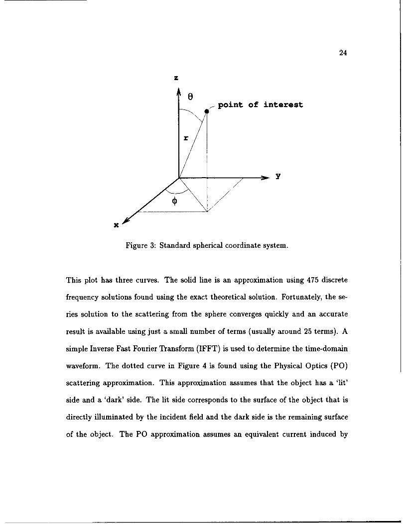
The standard spherical coordinate system is used in the following sections and is
sketched in Figure 3. It also must be pointed out that this analysis concentrates
on the high-frequency scattering of a structure. As stated before, high-frequency
implies that the overall size of an object is near or over one wavelength.
3.2.1 Point Scatterer
The point scatterer, by definition, scatters identically for all frequencies, angles, and
polarizations. Thus the model for this scattering center, which is a constant for both
frequency and angular dependencies, is simple and accurate.
3.2.2 Sphere
There is a theoretical solution for the scattering from the sphere [45]. This solution
is an infinite series which gives the backscattered field for one frequency of illumi-
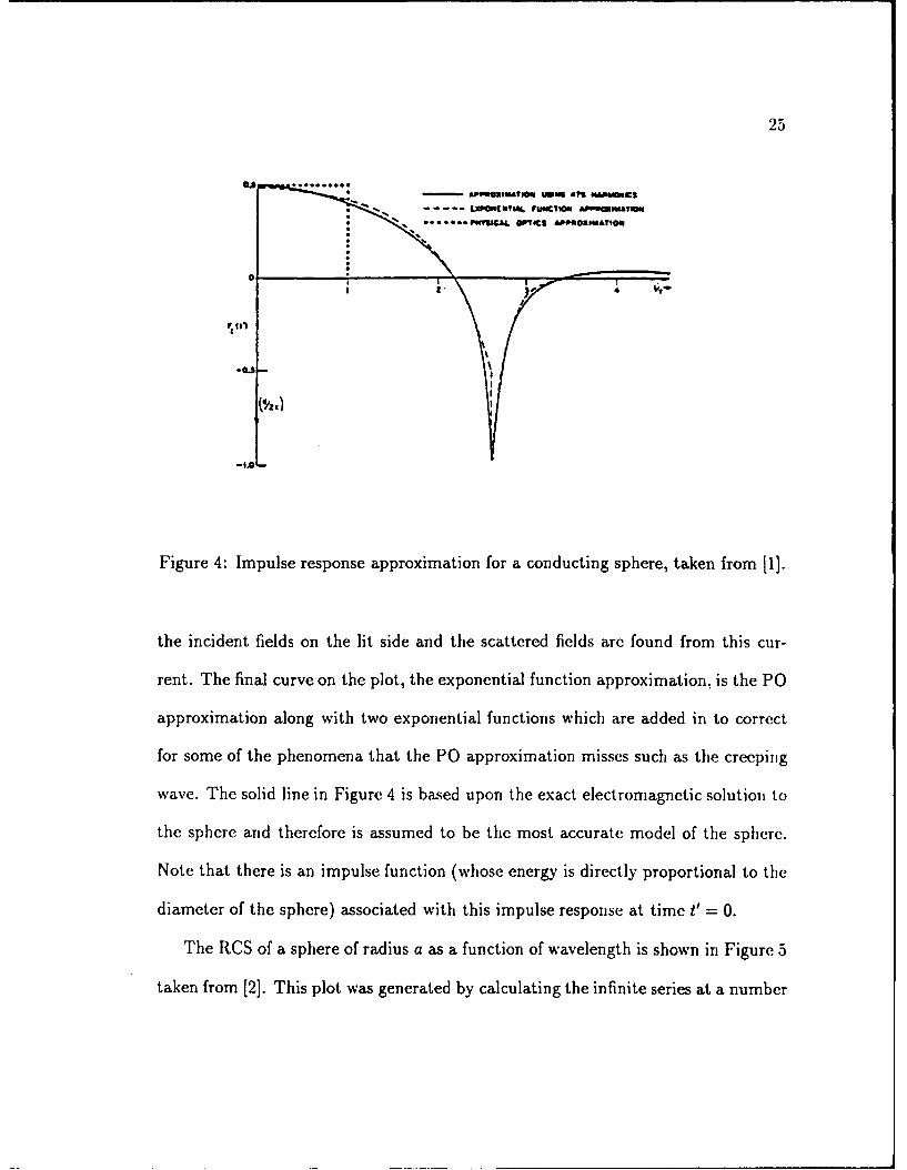
nation. The impulse response of the sphere is shown in Figure 4, taken from [1].
24
z
0point of interest
r
x
Figure 3: Standard spherical coordinate system.
This plot has three curves. The solid line is an approximation using 475 discrete
frequency solutions found using the exact theoretical solution. Fortunately, the se-
ries solution to the scattering from the sphere converges quickly and an accurate
result is available using just a small number of terms (usually around 25 terms). A
simple Inverse Fast Fourier Transform (IFFT) is used to determine the time-domain
waveform. The dotted curve in Figure 4 is found using the Physical Optics (PO)
scattering approximation. This approximation assumes that the object has a 'lit'
side and a 'dark' side. The lit side corresponds to the surface of the object that is
directly illuminated by the incident field and the dark side is the remaining surface
of the object. The PO approximation assumes an equivalent current induced by
25
.. ........... cspo-v*,
Figure 4: Impulse response approximation for a conducting sphere, taken from 11].
the incident fields on the lit side and the scattered fields are found from this cur-
rent. The final curve on the plot, the exponential function approximation, is the P0
approximation along with two exponential functions which are added in to correct
for some of the phenomena that the P0 approximation misses such as thle creeping
wave. Thle solid line in Figure 4 is based upon the exact electromagnetic solution, to
the sphere arid therefore is assumed to be the most accurate model of the sphere.
Note that there is an impulse function (whose energy is directly proportional to the
diameter of the sphere) associated with this impulse response at time 1' = 0.
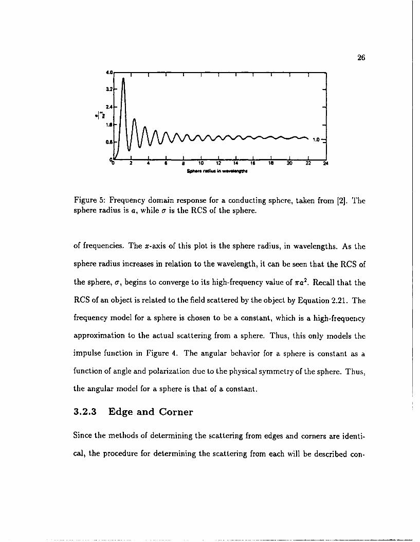
The RCS of a sphere of radius a as a function of wavelength is shown in Figure 5
taken from [2]. This plot was generated by calculating the infinite series at a number
26
.2-
2.4-
O.8 1.0-
2 4 6 a 10 12 14 16 18 20 22 24Sphm radka in wamaeqts
Figure 5: Frequency domain response for a conducting sphere, taken from [2]. Thesphere radius is a, while a is the RCS of the sphere.
of frequencies. The x-axis of this plot is the sphere radius, in wavelengths. As the
sphere radius increases in relation to the wavelength, it can be seen that the RCS of
the sphere, a, begins to converge to its high-frequency value of 7ra 2 . Recall that the
RCS of an object is related to the field scattered by the object by Equation 2.21. The
frequency model for a sphere is chosen to be a constant, which is a high-frequency
approximation to the actual scattering from a sphere. Thus, this only models tile
impulse function in Figure 4. The angular behavior for a sphere is constant as a
function of angle and polarization due to the physical symmctry of the sphere. Thus,
the angular model for a sphere is that of a constant.
3.2.3 Edge and Corner
Since the methods of determining the scattering from edges and corners are identi-
cal, the procedure for determining the scattering from each will be described con-
27
Edge/Corners
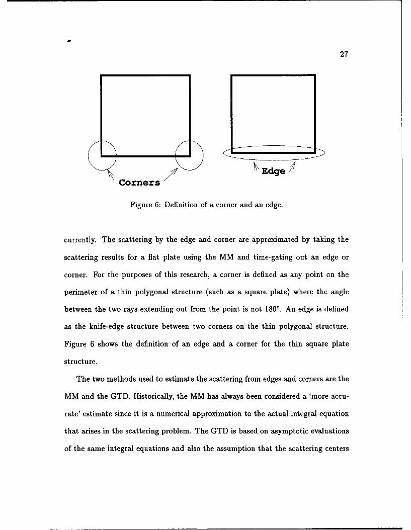
Figure 6: Definition of a corner and an edge.
currently. The scattering by the edge and corner are approximated by taking the
scattering results for a flat plate using the MM and time-gating out an edge or
corner. For the purposes of this research, a corner is defined as any point on the
perimeter of a thin polygonal structure (such as a square plate) where the angle
between the two rays extending out from the point is not 1800. An edge is defined
as the knife-edge structure between two corners on the thin polygonal structure.
Figure 6 shows the definition of an edge and a corner for the thin square plate
structure.
The two methods used to estimate the scattering from edges and corners are the
MM and the GTD. Historically, the MM has always been considered a 'more accu-
rate' estimate since it is a numerical approximation to the actual integral equation
that arises in the scattering problem. The GTD is based on asymptotic evaluations
of the same integral equations and also the assumption that the scattering centers
28
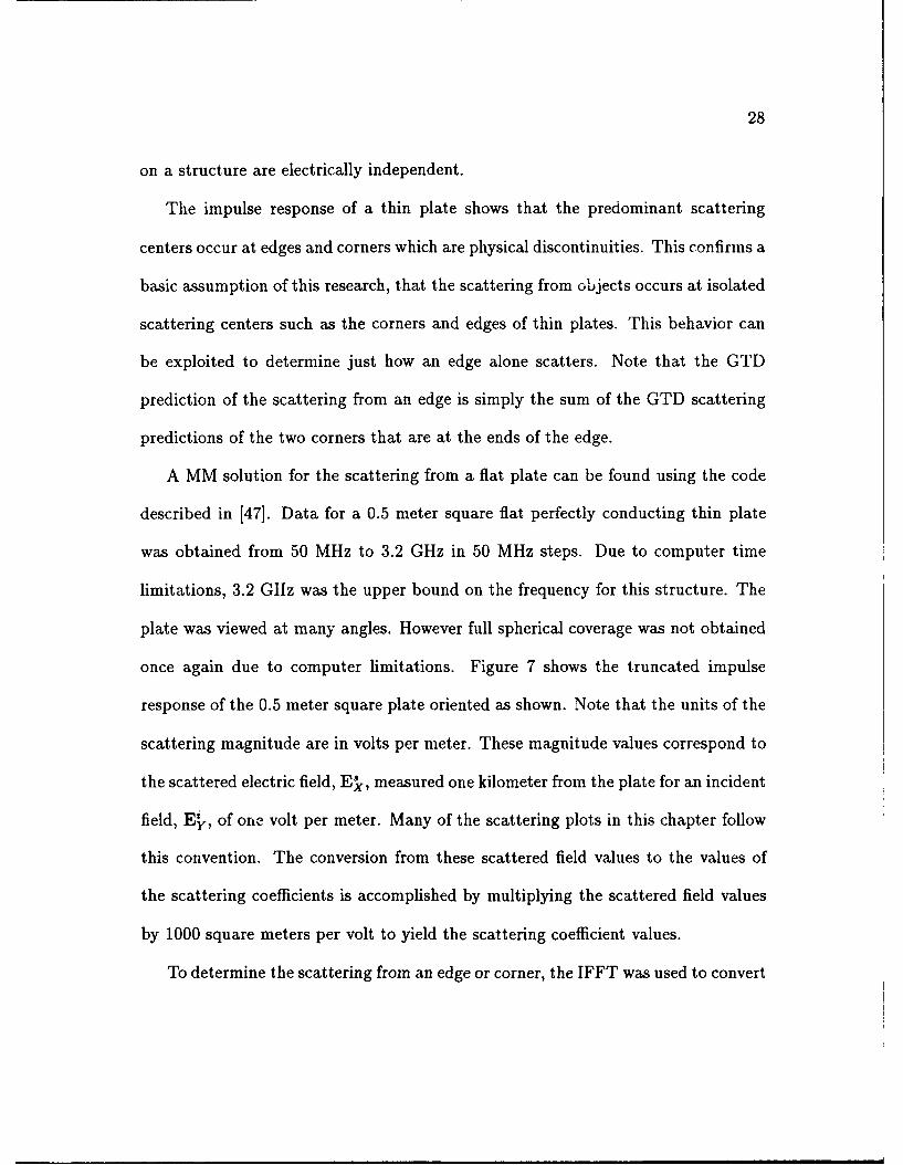
on a structure are electrically independent.
The impulse response of a thin plate shows that the predominant scattering
centers occur at edges and corners which are physical discontinuities. This confirms a
basic assumption of this research, that the scattering from objects occurs at isolated
scattering centers such as the corners and edges of thin plates. This behavior can
be exploited to determine just how an edge alone scatters. Note that the GTD
prediction of the scattering from an edge is simply the sum of the GTD scattering
predictions of the two corners that are at the ends of the edge.
A MM solution for the scattering from a flat plate can be found using the code
described in [47]. Data for a 0.5 meter square flat perfectly conducting thin plate
was obtained from 50 MHz to 3.2 GHz in 50 MHz steps. Due to computer time
limitations, 3.2 GHz was the upper bound on the frequency for this structure. The
plate was viewed at many angles. However full spherical coverage was not obtained
once again due to computer limitations. Figure 7 shows the truncated impulse
response of the 0.5 meter square plate oriented as shown. Note that the units of the
scattering magnitude are in volts per meter. These magnitude values correspond to
the scattered electric field, EX8, measured one kilometer from the plate for an incident
field, E , of one volt per meter. Many of the scattering plots in this chapter follow
this convention. The conversion from these scattered field values to the values of
the scattering coefficients is accomplished by multiplying the scattered field values
by 1000 square meters per volt to yield the scattering coefficient values.
To determine the scattering from an edge or corner, the IFFT was used to convert
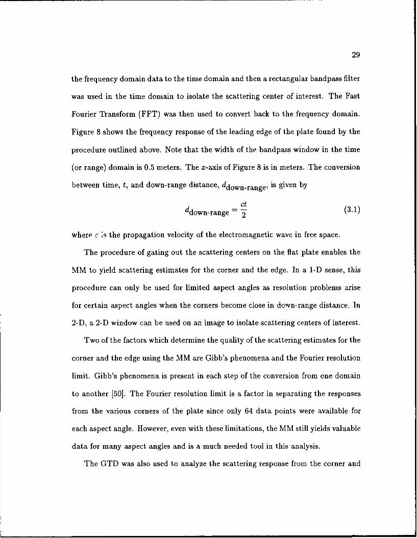
29
the frequency domain data to the time domain and then a rectangular bandpass filter
was used in the time domain to isolate the scattering center of interest. The Fast
Fourier Transform (FFT) was then used to convert back to the frequency domain.
Figure 8 shows the frequency response of the leading edge of the plate found by the
procedure outlined above. Note that the width of the bandpass window in the time
(or range) domain is 0.5 meters. The x-axis of Figure 8 is in meters. The conversion
between time, t, and down-range distance, ddown-range, is given by
ct(3 1ddownrange 2t (3.1)
where c s the propagation velocity of the electromagnetic wave in free space.
The procedure of gating out the scattering centers on the fiat plate enables the
MM to yield scattering estimates for the corner and the edge. In a 1-D sense, this
procedure can only be used for limited aspect angles as resolution problems arise
for certain aspect angles when the corners become close in down-range distance. In
2-D, a 2-D window can be used on an image to isolate scattering centers of interest.
Two of the factors which determine the quality of the scattering estimates for the
corner and the edge using the MM are Gibb's phenomena and the Fourier resolution
limit. Gibb's phenomena is present in each step of the conversion from one domain
to another [50]. The Fourier resolution limit is a factor in separating the responses
from the various corners of the plate since only 64 data points were available for
each aspect angle. However, even with these limitations, the MM still yields valuable
data for many aspect angles and is a much needed tool in this analysis.
The GTD was also used to analyze the scattering response from the corner and
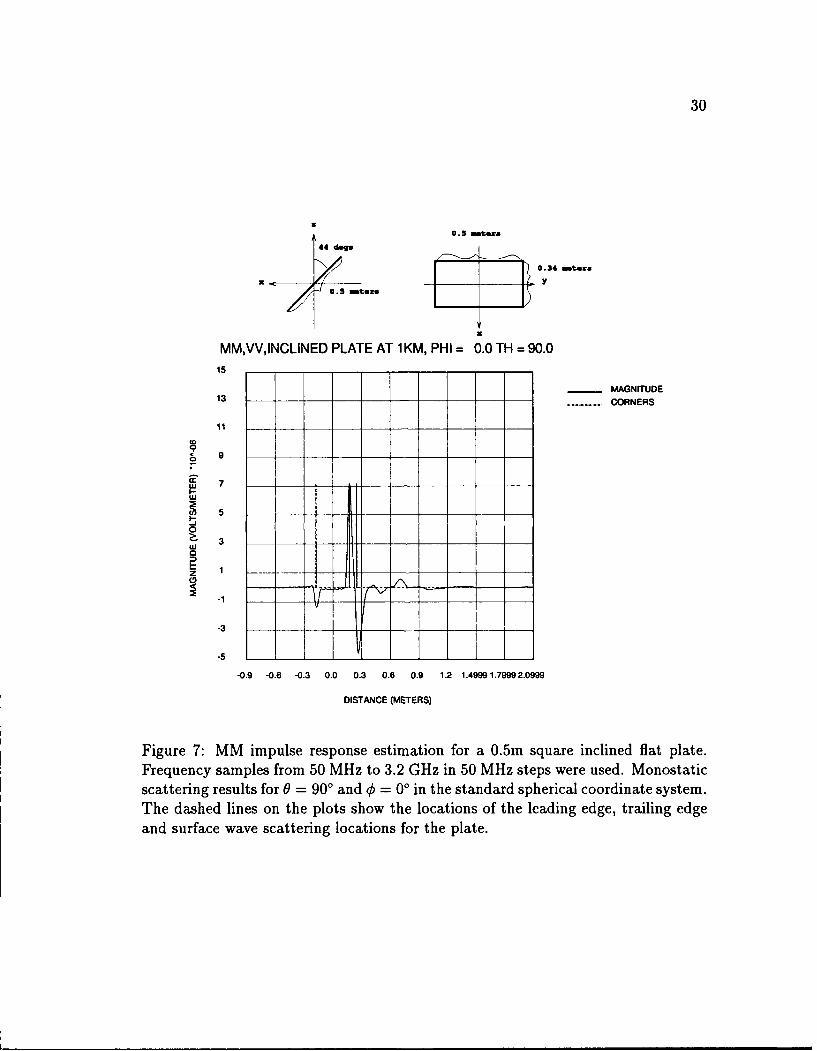
30
0.5 iters
44 deg
0.34 mete
N YS/ 0.5 inter-.
MM,VV,INCLINED PLATE AT 1KM, PHI = 0.0 TH = 90.0
15
13_ MAGNITUDE
13 . CORNERS
11 ...._____
5
0 9Z' 7
W
-5
-0.9 -0.6 -0.3 0.0 0.3 0.6 0.g 1.2 1.4M9 1.7M 2.0
DISTANCE (METERS)
Figure 7: MM impulse response estimation for a 0.5m square inclined flat plate.Frequency samples from 50 MHz to 3.2 GHz in 50 MHz steps were used. Monostaticscattering results for 0 = 900 and 4) = 00 in the standard spherical coordinate system.The dashed lines on the plots show the locations of the leading edge, trailing edgeand surface wave scattering locations for the plate.
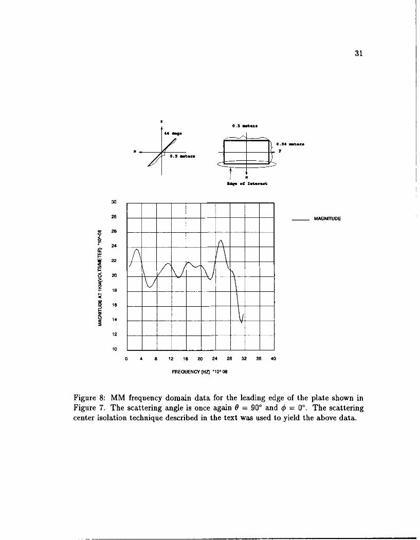
31
3O3
0..5 3 =etarz
0.53 itezz
Zdg o neres
30
28 MAGNITUDE
CO 269
24
w
I-LU22__
~20 _f V
C-
o 18
1112_____ j10
0 4 8 12 16 20 24 28 32 36 40
FREQUENCY (HZ) 10A 08
Figure 8: MM frequency domain data for the leading edge of the plate shown inFigure 7. The scattering angle is once again 0 = 90' and 0 = 00. The scatteringcenter isolation technique described in the text was used to yield the above data.
32
the edge. The resolution problems associated with the MM solution are avoided
by using the GTD. One of the useful features of the GTD and RCS-BSC 2.0 [49]
is that the response for one corner of a plate can be found directly. The GTD
determines the scattering from a structure by first calculating the scattering from
each component, such as a corner or an edge, and then adds all of the components
together to determine the overall scattering of the structure. Thus, the scattering
from each component can be found directly, and the procedure of filtering to isolate
scattering centers is not needed. This avoids the problems of Gibb's phenomena and
the truncation of overlapping responses.
The GTD response for the edge of Figure 8 is shown in Figure 9. Figure 9 was
generated using the computer code RCS-BSC 2.0. Note that the edge is basically
a constant as a function of frequency for frequencies where the plate is over one
wavelength in size, which is the region where the GTD results are accurate. Figure 10
is the frequency response of a corner as calculated by GTD. Figure 11 is the frequency
response of the same corner found by using the MM, range gating and using the FFT
as described earlier. From the GTD based corner scattering estimate, the frequency
response of the corner is , where w is the radian frequency. The MM estimate
follows this behavior for part of the bandwidth selected in Figure 11. Around the
ends of the bandwidth for the MM estimate, the response does not follow the I
behavior. Gibb's phenomena may account for this due to the windowing required to
isolate the corner in the range domain. Thus, the frequency behavior for the corner
is estimated to be for all aspect angles and all polarizations. Thus, this frequency
33
0. 5 uster
44 dsq.
0. 34 enter$
0.3 aser
24g. of Itrs
MAGNITUDE
GTD2,W, 0.5M SQ. PLATE AT 1KM, PHI = 0.0TH = 90.090
82
74
66
- 58
50-j0; 42 w
z- 34
26 _
18 _
10
0 3 6 9 12 15 18 21 24 27 30
FREQUENCY (MHZ) -10A 03
Figure 9: GTD impulse response estimation for the leading edge of the plate shownin Figure 7. Once again, the scattering angle is 0 = 900 and ¢ = 00.
34
behavior is polarization independent. It is also true that the frequency behavior of
an edge is also polarization independent.
Now that the frequency behavior of the edge and corner have been examined,
their angular behavior will be examined. The corner and the edge exhibit highly
variable angular behavior as shown in Figures 12, 13, and 14. Note that the scat-
tering magnitudes in these plots are expressed in RCS, in units of dB relative to a
square meter (DBSM). One noticeable characteristic is that there is a large jump in
the scattered field when the radar approaches one of the edges that makes up the
corner (that is 0 = 00, 900, 1800, and 270'). The angles which are parallel with one
of the edges that defines a corner will be called the 'grazing' angles. For the regions
in-between these grazing angles, the angular response is almost constant.
For the edge, the scattering is relatively constant for angles of which are not
perpendicular or parallel to the edge. For angles which are perpendicular or paral-
lel to the edge, which are designated the grazing angles for the edge, the angular
behavior is impulsive. Thus, the angular model for these scatterers will thus reflect
two types of corners and edges, one with a constant angular behavior and one with
an impulsive angular behavior.
3.2.4 Dihedral
A dihedral is sketched in Figure 15. The frequency response amplitude of a dihedral
is proportional to frequency to the first power, or w, for incident angles which look
into the interior of the dihedral. This is illustrated in Figure 16 taken from [3] which
used the GTD. The predominant scattering mechanism occurs at the apex of the
35
0.5 mt.r44 dogas C2 ;/ 2
0. 34 inters
0. nera
C4 C3
X
MAGNITUDE
GTD2,W, 0.5M SQ. PLATE AT 1KM, PHI = 45.0 TH 90.010
9
8
9 S7
6
0?- 4 _0
2 _
0
0 3 6 9 12 15 18 21 24 27 30
FREQUENCY (MHZ) 10OA 03
Figure 10: GTD frequency response estimation for the leading right corner (C3) ofthe plate shown in Figure 7. The scattering angle is fixed at 0 = 900 and =450.
Frequency domain data extends from 50 MHz to 20 GHz in 50 MHz steps.
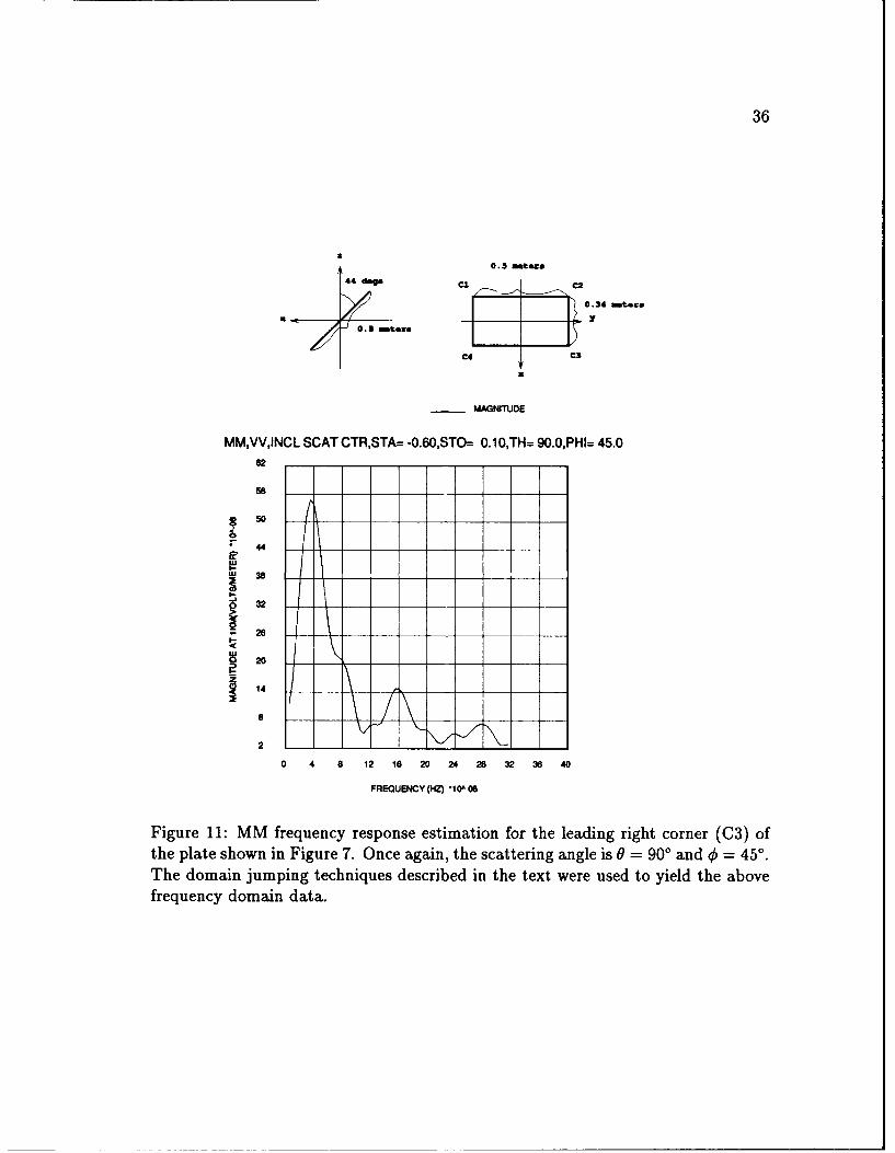
36
0.5 m3er
44 dmg Ci C2
0. 34 intown
-Y
CM C
_ MAGNITUDE
MM,VV,INCL SCAT CTR,STA= -0.60,STO= 0.10,TH= 0.0,PHI= 45.062
6
50
44
2o
14 0 64
0 4 a 12 18 20 24 28 32 38 40
FREQUENCY (HZ) '10 08
Figure 11: MM frequency response estimation for the leading right corner (C3) ofthe plate shown in Figure 7. Once again, the scattering angle is 0 = 900 and 40 = 45' .
The domain jumping techniques described in the text were used to yield the abovefrequency domain data.
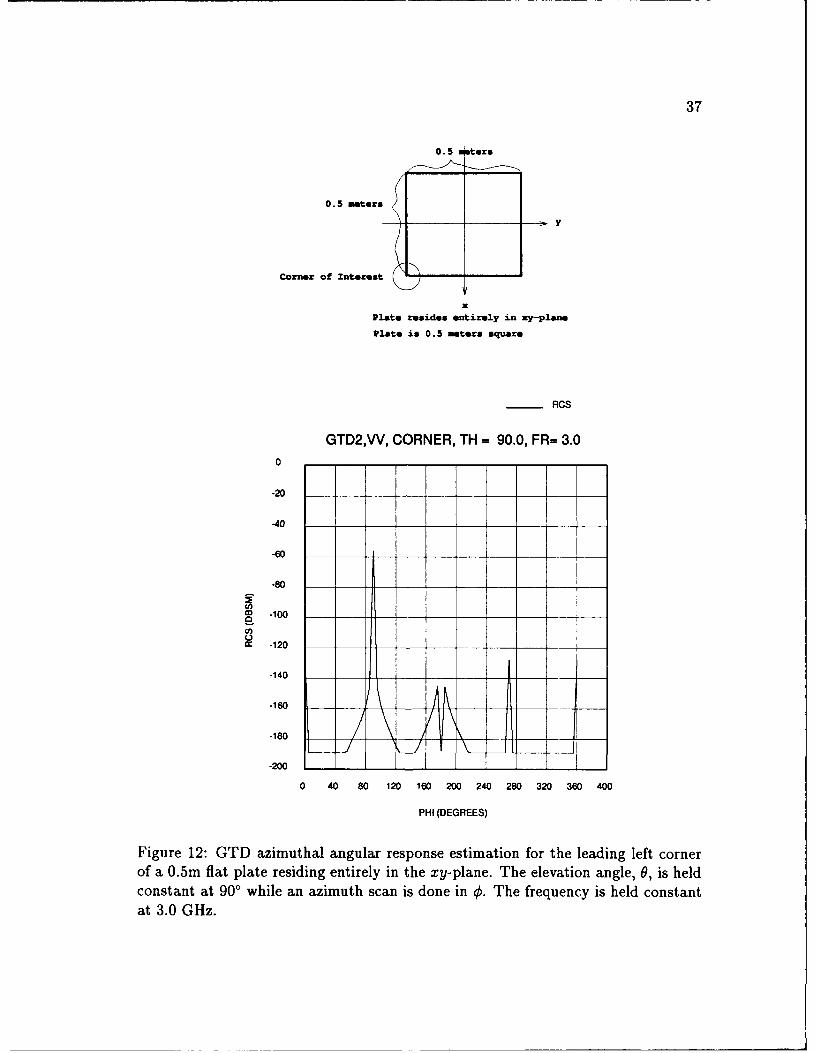
37
0.5 moters
0.5 meters
Corner of Xnterest
Plate resides entirely in zy-plane
Plate is 0.5 meters square
__ RCS
GTD2,VV, CORNER, TH = 90.0, FR= 3.0
-20
-40
-60
-80
co-120
-140
-160 _
-180 ___
-200
0 40 80 120 160 200 240 280 320 360 400
PHI (DEGREES)
Figure 12: GTD azimuthal angular response estimation for the leading left cornerof a 0.5m flat plate residing entirely in the xy-plane. The elevation angle, 0, is heldconstant at 900 while an azimuth scan is done in q. The frequency is held constantat 3.0 GHz.
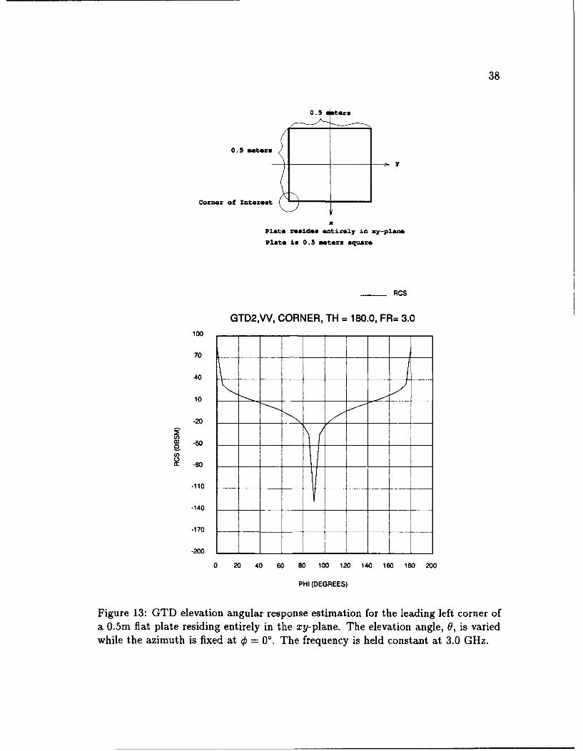
38
0.5 mtors
0. 5 motors
Corner of Xnterest
Plate resides entirely in 3W-planePlate is 0.5 mters square
____ RCS
GTD2,W(, CORNER, TH =180.0, FR= 3.0100 - - - -- _ _ _
70 __ __ __ __
40 __ __
10 ___ __
-20 _
-80 _
-110___ _ _
-140
-170 _ _ _ _ _
-200
0 20 40 60 80 100 120 140 160 180 200
PHI (DEGREES)
Figure 13: GTD elevation angular response estimation for the leading left corner ofa 0.5m flat plate residing entirely in the xy-plane. The elevation angle, 0, is variedwhile the azimuth is fixed at 0 = 00. The frequency is held constant at 3.0 GHz.
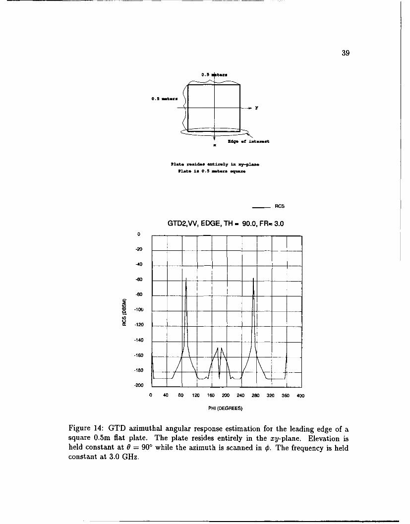
39
0. 5 atars
0.5. iner
Edge of intezetx
Plate resides entirely in zy-plasePlate is 0.5 moter square
RCS
GTD2,VV, EDGE, TH = 90.0, FR= 3.0
-20
-40
-60- - _
-80 -
C -100
c -120
-140
-160 AN_
-180 __ ____
-200 L
0 40 80 120 160 200 240 280 320 360 40
PHI (DEGREES)
Figure 14: GTD azimuthal angular response estimation for the leading edge of asquare 0.5m flat plate. The plate resides entirely in the xy-plane. Elevation isheld constant at 0 = 90' while the azimuth is scanned in 0. The frequency is heldconstant at 3.0 GHz.
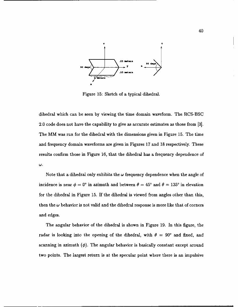
40
.25 meters90 dogs
.25 meters
smter.
Figure 15: Sketch of a typical dihedral.
dihedral which can be seen by viewing the time domain waveform. The RCS-BSC
2.0 code does not have the capability to give as accurate estimates as those from [3].
The MM was run for the dihedral with the dimensions given in Figure 15. The time
and frequency domain waveforms are given in Figures 17 and 18 respectively. These
results confirm those in Figure 16, that the dihedral has a frequency dependence of
w3.
Note that a dihedral only exhibits the w frequency dependence when the angle of
incidence is near 0 = 0' in azimuth and between 0 = 450 and 0 = 1350 in elevation
for the dihedral in Figure 15. If the dihedral is viewed from angles other than this,
then the w behavior is not valid and the dihedral response is more like that of corners
and edges.
The angular behavior of the dihedral is shown in Figure 19. In this figure, the
radar is looking into the opening of the dihedral, with 0 = 900 and fixed, and
scanning in azimuth (0). The angular behavior is basically constant except around
two points. The largest return is at the specular point where there is an impulsive
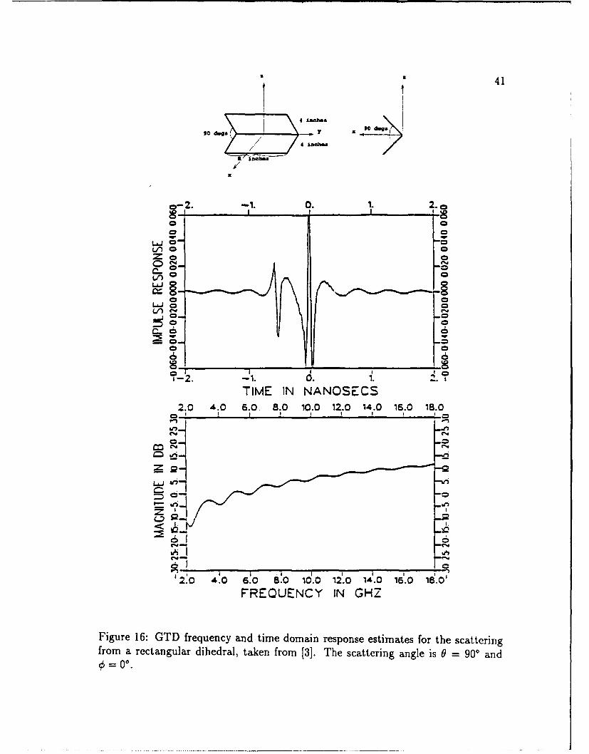
3 41
90 dogs, 9 z to
-2. 01. . 1.2.
o C
Z _ e
( -"C.
I I
S2.0 4.0 6.0 8.0 10.0 12..0 14.0 16.0 16.0
Ln
€=0° .
-0
'2.0 4.0 6.0. 8.0 10.0 12.0 14.0 16.0 18.0
= 00.
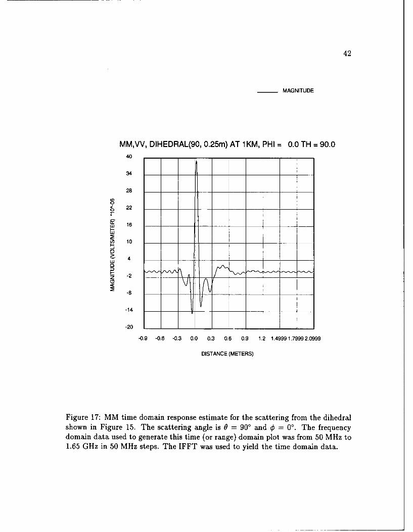
42
MAGNITUDE
MM,VV, DIHEDRAL(90, 0.25m) AT 1 KM, PHI = 0.0 TH = 90.0
40
34 _
28
to9
22
a 16
03 10 _I-.-J0
4 LU
Z -20
-8__
-14
-20
-0.9 -0.6 -0.3 0.0 0.3 0.6 0.9 1.2 1.4999 1.7999 2.0999
DISTANCE (METERS)
Figure 17: MM time domain response estimate for the scattering from the dihedralshown in Figure 15. The scattering angle is 0 = 900 and 4 = 00. The frequencydomain data used to generate this time (or range) domain plot was from 50 MHz to1.65 GHz in 50 MHz steps. The IFFT was used to yield the time domain data.
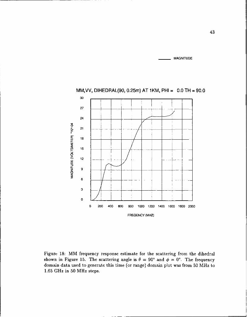
43
MAGNITUDE
MM,VV, DIHEDRAL(90, 0.25m) AT 1KM, PHI = 0.0 TH = 90.030
27
24 / ____ _ _ _
I-
21
V35 15 _ _
w 12
Z.- 9
6
0 200 400 600 800 1000 1200 1400 1600 1800 2000
FREQIENCY (MHZ)
Figure 18: MM frequency response estimate for the scattering from the dihedralshown in Figure 15. The scattering angle is 0 = 90' and 4 = 00. The frequencydomain data used to generate this time (or range) domain plot was from 50 MHz to1.65 GHz in 50 MHz steps.
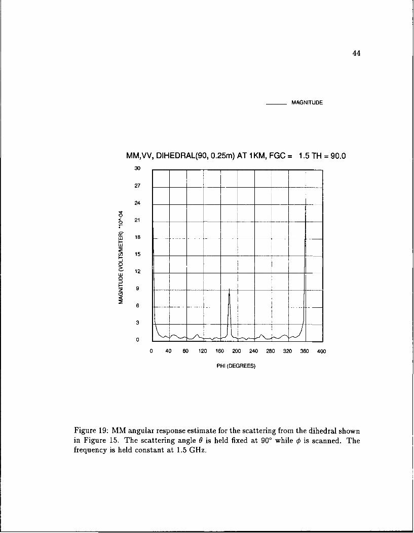
44
____MAGNITUDE
MM,VV, DIHEDRAL(90, 0.25m) ATl1KM, FGC = 1.5 TH =90.0
30
27 __ __
241 _ _
S 21 __
15 __ _
012 __
0
6.
0 40 80 120 160 200 240 280 320 360 400
PHI (DEGREES)
Figure 19: MM angular response estimate for the scattering from the dihedral shownin Figure 15. The scattering angle 0 is held fixed at 900 while (k is scanned. Thefrequency is held constant at 1.5 GHz.
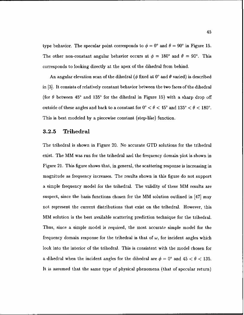
45
type behavior. The specular point corresponds to q5 = 00 and 9 = 900 in Figure 15.
The other non-constant angular behavior occurs at b = 1800 and 0 = 900. This
corresponds to looking directly at the apex of the dihedral from behind.
An angular elevation scan of the dihedral (0$ fixed at 00 and 0 varied) is described
in [3]. It consists of relatively constant behavior between the two faces of the dihedral
(for 9 between 450 and 1350 for the dihedral in Figure 15) with a sharp drop off
outside of these angles and back to a constant for 00 < 9 < 450 and 1350 < 0 < 1800.
This is best modeled by a piecewise constant (step-like) function.
3.2.5 Trihedral
The trihedral is shown in Figure 20. No accurate GTD solutions for the trihedral
exist. The MM was run for the trihedral and the frequency domain plot is shown in
Figure 21. This figure shows that, in general, the scattering response is increasing in
magnitude as frequency increases. The results shown in this figure do not support
a simple frequency model for the trihedral. The validity of these MM results are
suspect, since the basis functions chosen for the MM solution outlined in [47] may
not represent the current distributions that exist on the trihedral. However, this
MM solution is the best available scattering prediction technique for the trihedral.
Thus, since a simple model is required, the most accurate simple model for the
frequency domain response for the trihedral is that of w, for incident angles which
look into the interior of the trihedral. This is consistent with the model chosen for
a dihedral when the incident angles for the dihedral are 0 = 0' and 45 < 9 < 135.
It is assumed that the same type of physical phenomena (that of specular return)

46
Point is into the page
Figure 20: Definition of a trihedral.
occurs for the trihedral for viewing angles which are looking into the interior of the
trihedral that occurs for the dihedral when the viewing angles of the dihedral are at
= 0' and 45 < 0 < 135.
The angular behavior of the trihedral is shown in Figure 22. This behavior
suggests that the scattering is much larger when the radar is looking into the concave
(or interior) structure of the trihedral than it is when the radar is not. Over the
viewing angles that look into the concave structure of the trihedral, the scattering
behavior is nearly constant. The scattering behavior is also somewhat constant over
the other regions (but much lower). This suggests the angular model of a piecewise
constant (step-like) function.
3.2.6 Flat Plate
The flat plate can be described by the sum of the responses of the edges and corners
which comprise the plate for almost all aspect angles. One physical phenomena
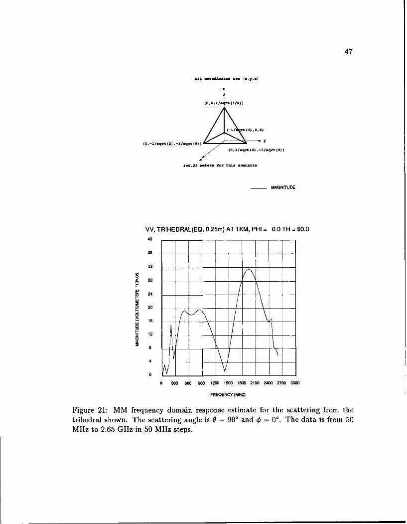
47
All oerLdnates are (x,y,s)
3
(0,,.1/ xt(3/2))
(-l/ C)0O
(0,-2/oqzt(2),-l/sqrt(G)) . -
(0, l/sqrt (2) ,-1/sqrt (6) )
1-0.25 mtrea for this sonertxo
_ MAGNITUDE
VV, TRIHEDRAL(EQ, 0.25m) AT 1KM, PHI = 0.0 TH = 90.040
38_
32
928
, 2 4
0?16
Z 12
8
4I
00 300 600 900 1200 1500 1800 2100 2400 2700 3000
FREQENCY (MHZ)
Figure 21: MM frequency domain response estimate for the scattering from thetrihedral shown. The scattering angle is 0 = 900 and € = 00. The data is from 50MHz to 2.65 GHz in 50 MHz steps.
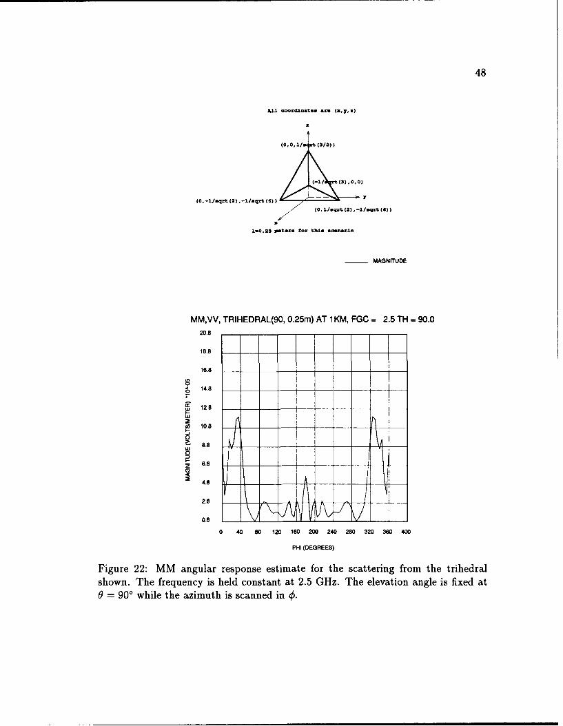
48
&11 aordinaiss are (z, y, x)
(0, 0,1/04X (3/2))
(-1/ (3).0,0)
(0,-1IsqrtC2),-1Isqrt(G)) --
Z (0, 11.qzt (2), -1/oqrzt (6))
1.0.23 :stoe. for this Ponalo
___ MAGNITUDE
MM,VV, TRIHEDRAL(90, 0.25m) AT 1KM, FGC = 2.5 TH =90.0
16.8
S14.8 __
W 12.8
10.8 __ - -_ _
8.8 ___ 'A __
0
4.8
2.8
0.8 :
0 40 80 120 160 200 240 280 320 360 400
PHI (DEGREES)
Figure 22: MM angular response estimate for the scattering from the trihedralshown. The frequency is held constant at 2.5 GHz. The elevation angle is fixed at0 = 900 while the azimuth is scanned in 0.

49
z
Broadside incidence
-z direction
/y
x
Flat plate in xy-plane
Figure 23: Broadside angle of incidence off of a flat plate.
associated with the flat plate is called the specular reflection. The specular reflection
is i.egligible in magnitude, compared to the returns off the edges and corners of the
plate, except around one angle of incidence. This angle of incidence is the one which
is perpendicular to the flat face of the plate as shown in Figure 23. This angle will
be called the broadside angle.
The GTD prediction of the scattering from a plate at broadside is shown in
Fig are 24. It is clear from tl's plot that the scattering from the flat plate at broadside
is directly proportional to w. The MM was used and confirmed this behavior. This
behavior is only valid for a very small angular region around broadside. For angles
off broadside, the energy associated with the specular phenomena is scattered in
50
directions other than the backscatter direction. Based on this information, the
frequency model for the fiat plate will be w while the angular response will be 5 (0).
3.2.7 Cylinder
The cylinder is the final canonical scattering center to be analyzed. A cylinder is
sketched in Figure 25. An exact series solution for the scattering from an infinite
circular cylinder [45] (infinite in the z-direction in Figure 25, finite in radius) exists
for limited aspect angles. From [45], the frequency domain behavior for the cylinder
is that of v/§ for angles of incidence in the xy-plane in Figure 25. For angles of
incidence between 9 = 0° and 9 = 900 in Figure 25, the behavior is that of * [51].
For 0 = 00, the cylinder is a flat circular plate which has a frequency response of
w. The angular characteristics of the cylinder are constant for scans in .0 due to the
physical symmetry of the problem. As for scans in 9, the cylinder will be modeled
with a 6 (0) function at 9 = 00 and 0 = 900 and a constant function between 9 = 00+
and 0 = 90'- .
3.3 Summary of Scattering Characteristics for CanonicalScattering Centers
Table 1 is a summary of the frequency and angular models of the canonical scattering
centers discussed in the previous section. The analyses presented in the previous
section were used to determine the models in Table 1 based on two main criteria. The
first is that the models are based upon electromagnetic theory. Second, the models
must be simple enough to be used in inverse scattering algorithms. In Table 1, w is
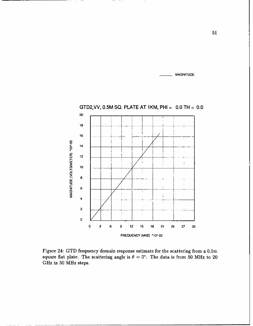
51
MAGNITUDE
GTD2,VV, 0.5M SQ. PLATE AT 1KM, PHI = 0.0 TH = 0.020
18 _ _ _ ______ _
16/
141
a: 12 __ ____ ___ _w
(A 10 __ __ __
0
0 i
I--z 6
4
2__
0
0 3 6 9 12 15 18 21 24 27 30
FREQUENCY (MHZ) 10A 03
Figure 24: GTD frequency domain response estimate for the scattering from a 0.5msquare flat plate. The scattering angle is 0 = 00. The data is from 50 MHz to 20GHz in 50 MHz steps.
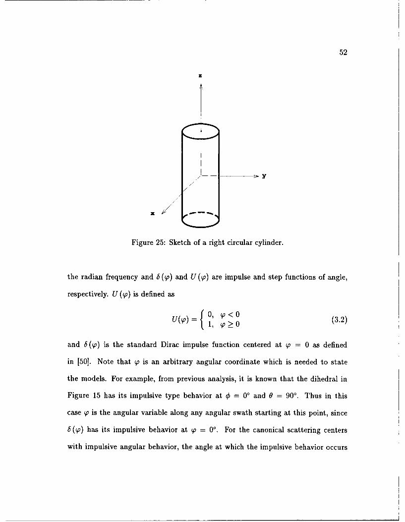
52
Figure 25: Sketch of a right circular cylinder.
the radian frequency and 6 ( o) and U ( o) are impulse and step functions of angle,
respectively. U (p) is defined as
S 0W<O (3.2)1, O> 0
and 6 (w) is the standard Dirac impulse function centered at W = 0 as defined
in [50]. Note that V is an arbitrary angular coordinate which is needed to state
the models. For example, from previous analysis, it is known that the dihedral in
Figure 15 has its impulsive type behavior at 4 = 0' and 9 = 900. Thus in this
case p is the angular variable along any angular swath starting at this point, since
b(p) has its impulsive behavior at V = 00. For the canonical scattering centers
with impulsive angular behavior, the angle at which the impulsive behavior occurs

53
Table 1: Approximate Frequency and Angle characteristics of canonical scatteringcenters.
Scatterer Frequency Dependence Angular Dependence
1. Point Scatterer, Sphere constant constant
2. Corner, no grazing1 constant3. Corner, grazing 1 6 (q)
4. Edge, no grazing nor I constant constant
5. Edge, grazing or I constant 6 ()
6. Dihedral, azimuth scan w 6 (0)
7. Dihedral, elevation scan w U ()
8. Trihedral w U ()
9. Cylinder, 0 = 900 6 ()
10. Cylinder, 00 < 0 < 90 '1 constant
11. Flat Plate (specular) w 6 ( )
12. Cylinder at 0 = 90' w 6 ()
corresponds to the W = 0' angle. Also, for the canonical scattering centers with a
step angular behavior, the angle at which the step behavior occurs corresponds to
the W = 0' angle. Of course, for the canonical scattering centers with a constant
angular behavior, the origin of the V coordinate is not fixed. Also note that 0 in
Table 1 is the 0 in the standard spherical coordinate system (as in Figure 25).
As mentioned before, this list is not all inclusive for all of the types of canonical
scattering centers which appear on all radar targets of interest. However, this list can
be expanded to include other canonical scattering centers. Also, scattering behavior
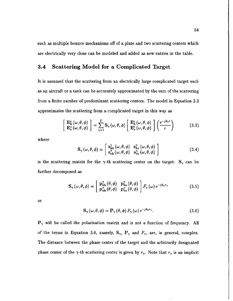
54
such as multiple bounce mechanisms off of a plate and two scattering centers which
are electrically very close can be modeled and added as new entries in the table.
3.4 Scattering Model for a Complicated Target
It is assumed that the scattering from an electrically large complicated target such
as an aircraft or a tank can be accurately approximated by the sum of the scattering
from a finite number of predominant scattering centers. The model in Equation 3.3
approximates the scattering from a complicated target in this way as
[ h ] ( ,, )0) [](3.3)E w, 0, 'Y=) -tl )
where
S7 (W, O,1) -- [ S h h P ' ) Sv (w', (, ] (3.4)
is the scattering matrix for the -y-th scattering center on the target. S7 can be
further decomposed as
S- 0,,) = P (h(, ') p 0 (O,¢) 1(p~h (,) p (0,) j F(w) e-jkoT (3.5)
or
S7 (w,9,¢) = P7Y (0, €) F- (w) e- o . (3.6)
P. will be called the polarization matrix and is not a function of frequency. All
of the terms in Equation 3.6, namely, S., P and F),, are, in general, complex.
The distance between the phase center of the target and the arbitrarily designated
phase center of the y-th scattering center is given by r.. Note that r', is an implicit
55
function of 0 and 0. It is assumed that there are r scattering centers on the target.
It is also worth noting that this is a full-polarization scattering model.
As shown above, for the canonical scattering centers analyzed in this chapter,
separating the frequency dependence from the remainder of the scattering matrix
is reasonable. However, separating the angular dependence from the rest of the
scattering matrix would be a poor assumption for canonical scattering centers such as
the corner and the edge. Of course, for physically symmetric scattering centers such
at a sphere, the angular dependence could be separated from the rest of the scattering
matrix. Most radar targets of interest contain many corners and edges, and thus a
model that separates the angular dependence from the rest of the scattering matrix
would be inappropriate.
3.5 Damped Exponential Modeling of Scattering Behaviorof Canonical Scattering Centers
The scattering behavior of the canonical scattering centers was outlined in Table 1.
These characteristics were electromagnetically derived. Later, in Chapter V the
scattering behavior of a complicated target, for a single transmit and receive polar-
ization, in the frequency and angle domains, is modeled by
F
d(m, n) = , p n (3.7)7,=1
where
pX- = -yth x-pole, x-component of 2-D exponential (complex number)
p , = -yth y-pole, y-component of 2-D exponential (complex number)
56
a.y = -yth amplitude coefficient (complex number)
F = number of scattering centers (integer)
and where m = 0-1...M-1 and n = 0,1,...N -1. This is the 2-D extension
of Prony's Model which is discussed in detail in Chapters V and VI. This model
assumes the complicated target is comprised of r scattering centers. The -Y-th
scattering center's scattering behavior, for a single transmit and receive polarization,
is modeled by the x-pole, y-pole and amplitude coefficient triple, {Pa,, pY, a-/}. The
magnitude of the damped exponential, lp, , determines the dispersion of the -y-th
scattering center in the x-coordinatk of the transform domain (time or range domain
in this case) while the angle of the damped exponential, /p,,, determines the location
of the -y-th scattering center in the x-coordinate of the transform domain. Similarly,
the magnitude of the damped exponential, IpyJ, determines the dispersion of the
-y-th scattering center in the y-coordinate of the transform domain while the angle of
the damped exponential, /py, determines the location of the -Y-th scattering centet
in the y-coordinate of the transform domain.
From Equations 3.3 and 3.6, a single polarization version for the scattering from
a complicated target is
r (__-E' (w,9,¢) 0 p(O, ¢)F 7 (w)E' (w, 0,9 ) (3.8)
X XY Y (r )
where x E {h,v}, y E {h,v} and xy E {hh, hv, vv}. Comparing Equations 3.7
and 3.8, the y-th individual scattering center's frequency and angular dependencies
are modeled by two damped exponentials, p, for the frequency dependence, and
pu for the angular dependence. Note that nere are two angular dependencies in
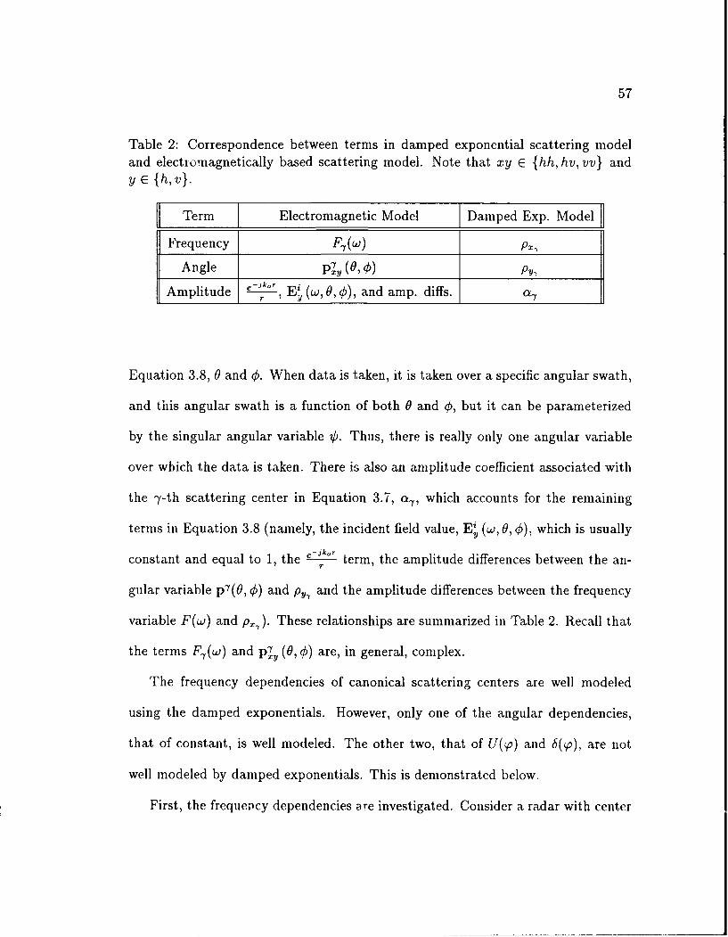
57
Table 2: Correspondence between terms in damped exponential scattering modeland electicmagnetically based scattering model. Note that xy E {hh, hv, vv} andy E {h,v}.
Term Electromagnetic Model Damped Exp. Model
Frequency F, (w) p_
Angle p'Y (0, ¢) j _ - _
Amplitude &-o, E' (w,0, ), and amp. diffs. a7
Equation 3.8, 0 and €. When data is taken, it is taken over a specific angular swath,
and this angular swath is a function of both 0 and ¢, but it can be parameterized
by the singular angular variable 0. Thus, there is really only one angular variable
over which the data is taken. There is also an amplitude coefficient associated with
the -f-th scattering center in Equation 3.7, a7 , which accounts for the remaining
terms in Equation 3.8 (namely, the incident field value, E' (w, 0, ¢), which is usually
constant and equal to 1, the e-kor term, the amplitude differences between the an-
gular variable pY(9, 0) and p., and the amplitude differences between the frequency
variable F(w) and p,). These relationships are summarized in Table 2. Recall that
the terms F7 (w) and p'y (0, ¢) are, in general, complex.
The frequency dependencies of canonical scattering centers are well modeled
using the damped exponentials. However, only one of the angular dependencies,
that of constant, is well modeled. The other two, that of U(o) and 6 ( o), are not
well modeled by damped exponentials. This is demonstrated below.
First, the frequepcy dependencies are investigated. Consider a radar with center
58
frequency 10 GHz and a bandwidth of 2 GHz. Scatterinb data is generated in the
1-D frequency domain of the form
dfr) =w?1 0,1,..20 (3.9)
where w and q] are related by
w = 2irr7(50MHz) + 27r(9.0GHz), (3.10)
and also where t E {-1,-, 0,1 1} (t is designated the "type" of the scattering
center) and where f = ranges from 9-11 GHz in 50 MHz steps, which yields 21
data points. This corresponds to a scattering center located at the origin of the
transform domain (range or time domain) since the complex phase of the data is
zero. Thus, wt represents all of the possible frequency dependencies from Table 1
that can appear in Equation 3.8. Next, consider the simple 1-D damped exponential
model of a single canonical scattering center,
d(n)= pn , n=0,1,...20. (3.11)
The 1-D TLS-Prony parameter estimation algorithm described in Chapter IV was
used to estimate the parameters a and p from the data dj(q?). Figures 26 through 28
show how well the damped exponential models all the frequency dependencies in
Table 1 over this radar bandwidth. Table 3 gives the parameter estimates for p
and a along with the relative error (RE) between the actual F(w) and the damped
exponential estimate for each of the F(w)'s. The RE is calculated by
RE- [ df(0) d(1) ... df(20) ]-[ d(0) d(1) ... d(20)]ll (3.12)I1[ df(0) df(1) ... df(20) ]11
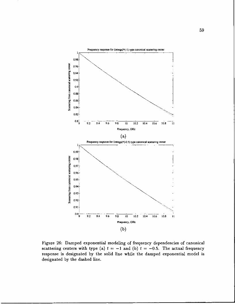
59
Frequency response for (omega)A(-) type canonical scattering center
0.98.
. 0.96-
.94
0.92-2
S0.9-
20.88-
0.86
g 0.84
0.82
0.89 9.2 9.4 9.6 9.8 10 10.2 10.4 10.6 10.8 11
Frequency, GHz
(a)Frequency response for (omega)A(-0.5) type canonical scattering center1 1
0.99
0.98 I.) 0.97
0.96,
0.9410
0.93 _ _ _ _ _ _
0.91 '"___
0.9 -
9 9.2 9.4 9.6 9.8 10 10.2 10.4 10.6 10.8 11
Frequency, GHz
(b)
Figure 26: Damped exponential modeling of frequency dependencies of canonicalscattering centers with type (a) t = -1 and (b) t = -0.5. The actual frequencyresponse is designated by the solid line while the damped exponential model isdesignated by the dashed line.
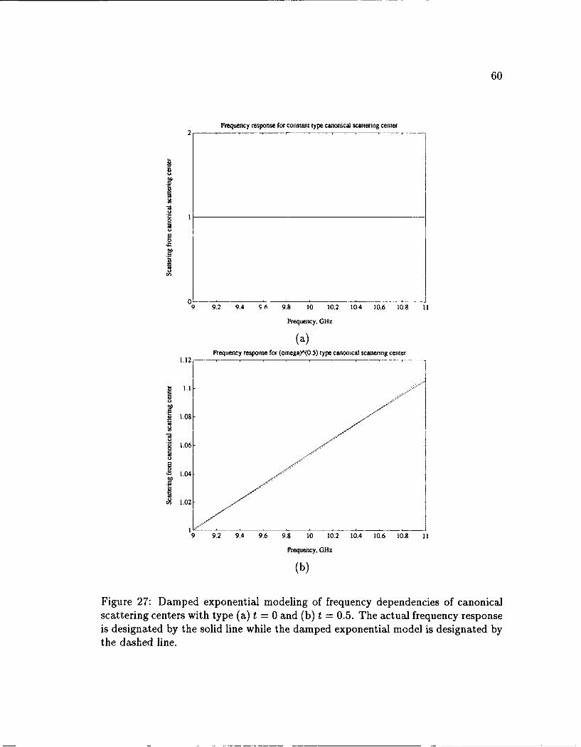
60
Frequency response for constant type canonical scattering center2
.9
00
9 9.2 9.4 96 9.8 10 10.2 10.4 10.6 10.8 11
Frequency, GHz
(a)Frequency response for (omega)A(0.5) type canonical scattering center
1.12
1.08
"* 1.06
1.04.511.02
9 9.2 9.4 9.6 9.8 10 10.2 10.4 10.6 10.8 11
Frequency, GHz
(b)
Figure 27: Damped exponential modeling of frequency dependencies of canonicalscattering centers with type (a) t = 0 and (b) t = 0.5. The actual frequency responseis designated by the solid line while the damped exponential model is designated bythe dashed line.
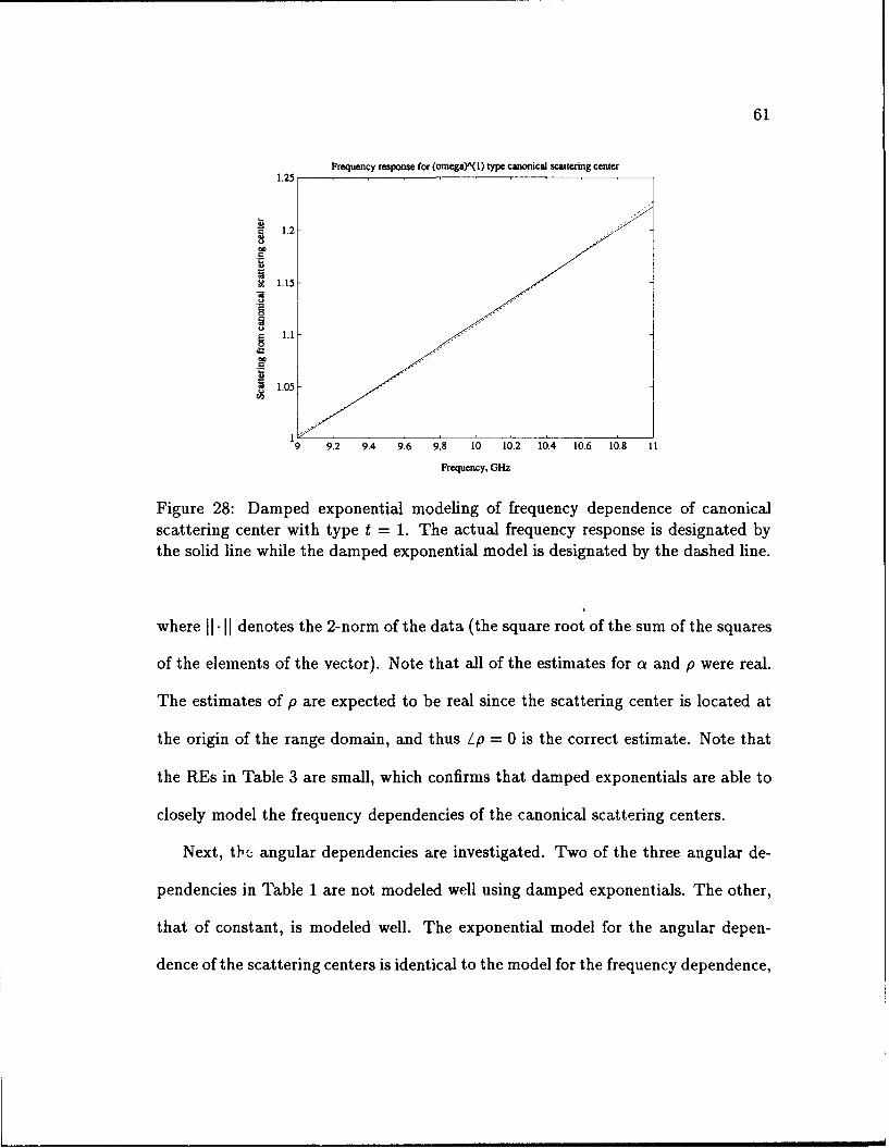
61
Frequency response for (omega)A(l) type canonical scattering center1.25
1.2
1I 1.15
S 1.1
.01.05
9 9.2 9.4 9.6 9.8 10 10.2 10.4 10.6 10.8 11
Frequency, GHz
Figure 28: Damped exponential modeling of frequency dependence of canonicalscattering center with type t = 1. The actual frequency response is designated bythe solid line while the damped exponential model is designated by the dashed line.
where denotes the 2-norm of the data (the square root of the sum of the squares
of the elements of the vector). Note that all of the estimates for a and p were real.
The estimates of p are expected to be real since the scattering center is located at
the origin of the range domain, and thus /p = 0 is the correct estimate. Note that
the REs in Table 3 are small, which confirms that damped exponentials are able to
closely model the frequency dependencies of the canonical scattering centers.
Next, thb angular dependencies are investigated. Two of the three angular de-
pendencies in Table 1 are not modeled well using damped exponentials. The other,
that of constant, is modeled well. The exponential model for the angular depen-
dence of the scattering centers is identical to the model for the frequency dependence,
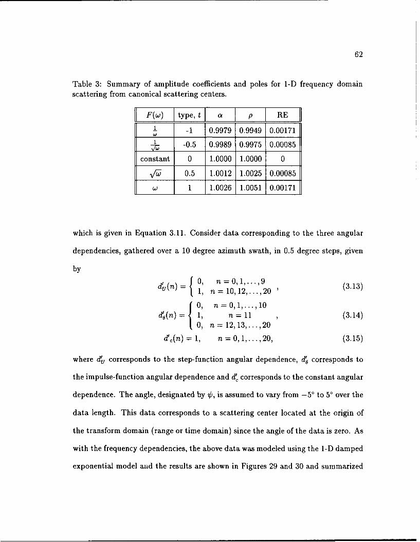
62
Table 3: Summary of amplitude coefficients and poles for 1-D frequency domainscattering from canonical scattering centers.
F(w) type, t a p RE
1 -1 0.9979 0.9949 0.00171
-0.5 0.9989 0.9975 0.00085
constant 0 1.0000 1.0000 0
VG 0.5 1.0012 1.0025 0.00085
w 1 1.0026 1.0051 0.00171
which is given in Equation 3.11. Consider data corresponding to the three angular
dependencies, gathered over a 10 degree azimuth swath, in 0.5 degree steps, given
by
d'(n)={ 0, n=0, 9 (3.13)U 1, n = 10, 12,..., 20
0, n -- 0,1,..10
d6(n) = 1, n- 11 , (3.14)1 0, n = 12, 13, ... ,120
d',(n) = 1, n = 0,1,..., 20, (3.15)
where d' corresponds to the step-function angular dependence, d' corresponds to
the impulse-function angular dependence and d, corresponds to the constant angular
dependence. The angle, designated by V, is assumed to vary from -5' to 50 over the
data length. This data corresponds to a scattering center located at the origin of
the transform domain (range or time domain) since the angle of the data is zero. As
with the frequency dependencies, the above data was modeled using the 1-D damped
exponential model and the results are shown in Figures 29 and 30 and summarized
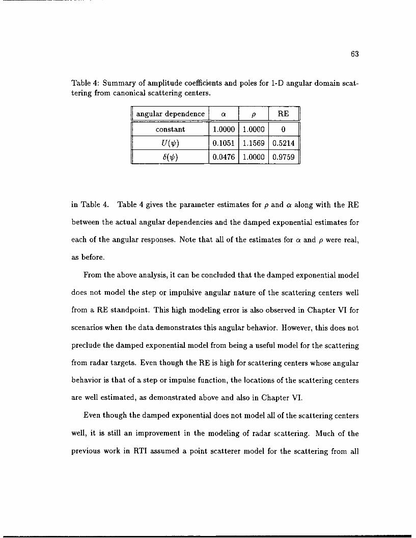
63
Table 4: Summary of amplitude coefficients and poles for 1-D angular domain scat-tering from canonical scattering centers.
1 angular dependence a p RE
constant 1.0000 1.0000 0
U(V)) 0.1051 1.1569 0.5214
0.0476 1.0000 0.9759
in Table 4. Table 4 gives the parameter estimates for p and a along with the RE
between the actual angular dependencies and the damped exponential estimates for
each of the angular responses. Note that all of the estimates for a and p were real,
as before.
From the above analysis, it can be concluded that the damped exponential model
does not model the step or impulsive angular nature of the scattering centers well
from a RE standpoint. This high modeling error is also observed in Chapter VI for
scenarios when the data demonstrates this angular behavior. However, this does not
preclude the damped exponential model from being a useful model for the scattering
from radar targets. Even though the RE is high for scattering centers whose angular
behavior is that of a step or impulse function, the locations of the scattering centers
are well estimated, as demonstrated above and also in Chapter VI.
Even though the damped exponential does not model all of the scattering centers
well, it is still an improvement in the modeling of radar scattering. Much of the
previous work in RTI assumed a point scatterer model for the scattering from all
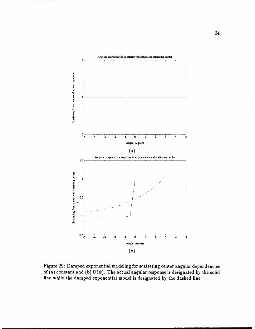
64
Angular response for constant type canonical scattering center2
.g 1' 0
0-5 -4 -3 -2 - 0 1 2 3 4 5
Angle, degrees
(a)Angular response for step function type canonical scattering center
1.5
bi
0.5 -
EI ---
00
-0.5 L _-5 -4 -3 -2 -1 0 1 2 3 4 5
Angle, degrees
(b)
Figure 29: Damped exponential modeling for scattering center angular dependenciesof (a) constant and (b) U(?). The actual angular response is designated by the solidline while the damped exponential model is designated by the dashed line.
65
Angular response for impulse function type canonical scattermg center1.5
* 0.5
------------------------ -- -....-. .---.. ... - --------------------------------------0
-0.5-5 -4 -3 -2 -1 0 1 2 3 4 5
Angle, degrees
Figure 30: Damped exponential modeling for scattering center angular dependenceof 6(Ob). The actual angular response is designated by the solid line while the dampedexponential model is designated by the dashed line.
types of canonical scattering centers [34], [35], [39]. The extension to a 2-D damped
exponential model is an improvement over the point scatterer model.
3.6 Summary
In this chapter the scattering characteristics of several canonical scattering centers
were examined. Techniques such as The Method of Moments (MM) and The Ge-
ometrical Theory of Diffraction (GTD) along with others were used to determine
the scattering characteristics of structures such as the edge, corner, dihedral, tri-
hedral and cylinder. The scattering characteristics of each canonical shape were
estimated as a function of frequency, radar-target orientation and polarization. The

66
high-frequency scattering model for a complicated radar target was defined, which
is the sum of the scattering responses from a finite number of canonical scattering
centers. The ability of a damped exponential model to accurately model the scatter-
ing characteristics of the canonical scattering centers was discussed in detail. The
use of a damped exponential is an improvement over the use of a point scatterer
model for the scattering from canonical scattering centers, as was done in much of
the previous work in RTI. It was concluded that the damped exponential models
the frequency responses of the canonical scattering centers well, but does not model
all of angular responses well. Scattering centers exhibiting impulsive or step angular
behavior are not well modeled utilizing a damped exponential. However, scattering
centers exhibiting constant angular behavior are well modeled utilizing a damped
exponential. This does not preclude the use of the 2-D damped exponential to model
the scattering from radar targets.
CHAPTER IV
Signal Processing Fundamentals
4.1 Background and Introduction
This research involves the analysis of multiple angle and multiple frequency radar
data. The analysis of 1-D multiple frequency radar data has been investigated for
many years [6]-[9]. One method of obtaining a down-range profile of the target
is to perform a simple Inverse Fast Fourier Transform (IFFT) on the frequency
domain data. Issues such as bandwidth, resolution and unambiguous range must
be considered using this approach. High resolution parametric techniques such as
ARMA modeling and Prony modeling can also be applied to the data. These models
are appropriate for data that contains localized peaks in the transform domain, as
is the case for most multiple frequency radar data.
The analysis of 2-D multiple frequency and multiple angle radar data has mainly
utilized the 2-D Fourier Transform [13]. These techniques are also applied in to-
mography and have applications in electron microscopy, x-rays, radio astronomy,
geology and medical imaging. The same issues involving bandwidth, sampling and
unambiguous range which exist in 1-D also exist in 2-D. High resolution parametric
techniques exist in 2-D [101, [52] and are appropriate for radar targets which have
67
68
range-domain profiles which contain localized scattering centers. Many radar tar-
gets do not have range domain profiles which fit this description, but parametric
techniques still may be appropriate in some of these cases.
First, 1-D techniques are described and some simple examples are shown. Then,
2-D techniques are introduced and several examples are shown.
4.2 One-Dimensional Techniques
It is assumed that we are given complex noisy 1-D data which has the form
d'(n) = d(n) + w(n), (4.1)
where n = 0, 1,..., N- 1, w (n) is the noise sequence and d (n) are the noiseless data.
Usually this data consists of the scattering coefficients as a function of frequency
which are also the scattered field values as a function of frequency at the radar (with
the e-kO° term removed) for a unity incident field (E' (f) = 1). All of the data
samples are taken with the radar-target orientation fixed. The frequency spacing
between samples is bf and thus the total bandwidth of the data is (N - 1) 6f. This
type of radar data is usually called stepped CW data (where the CW stands for
continuous wave). This refers to a radar measurement taken at a specific frequency
for CW illumination. The frequency of the radar is stepped to the next value and
another measurement is taken; this process is continued until all of the data is
collected. Radar data which is collected over a non-zero bandwidth, such as with
an FM ramp, can be used to approximate the stepped CW type of data.
The unambiguous range, R,, is the total size (in the range domain) that the
69
target must fit in to avoid aliasing. This is different than a more classical definition
for unambiguous range which involves the Pulse Repetition Frequency of a pulsed
radar. Thus, for this research the unambiguous range is related to bf by
CR,,- 2 I (4.2)
The 2 in the denomiiiator accounts for the two-way travel of the electromagnetic
wave. The Fourier resolution limit in the range domain is related to the bandwidth
(N - 1) 5 by
F~el- 2(N - 1)bf" (4.3)
The first method of obtaining a time-domain or down-range profile of the target
is to simply take the IFFT of the data. Recall that the IFFT is given by
N-1
D(1) = E d (n)e? 1 = 0,1,...,N - 1 (4.4)n=O
where {D'(1)}N- 1 are the time domain data. By properly scaling the time axis to
the range domain (as in Equation 3.1), the range domain profile can be obtained
from the data {D'(l)}ff=- 1 . Typically, the range profile plots in this dissertation are
plots of the magnitude of D'(1) versus range. Examples of these types of plots were
shown throughout Chapter III.
Examples using actual radar data are shown here in Figures 31 and 32. These
figures show the range domain profiles generated from data obtained at the compact
range at The ElectroScience Laboratory (ESL) at The Ohio State University. The
scattering object is an inclined flat plate which is sketched in Figure 31. Frequency
dom--n data was obtained from 2000 MHz to 17980 MHz in 20 MHz steps for hh
70
polarization. The 1-D FFT was used to transform the frequency domain data to
the range domain. Figure 31 shows the entire unambiguous range while Figure 32
shows only the section of the unambiguous range which contains the scattering from
the plate.
Bandwidth is an important factor in the processing of radar data. Obtaining
data over a large bandwidth is difficult as most radars operate over a relatively
small bandwidth (relative to the radar's center frequency). This is why parametric
techniques such as ARMA and Prony's Method are useful. These techniques can
achieve greater resolution than Fourier methods for the same bandwidth. Because
of this, if a resolution criterion is set, then parametric techniques require data over
a smaller bandwidth than that required by Fourier techniques.
Prony's Model is given by 1291
K
d(n)=akp'k, n=0, N. -1, (4.5)k=1
where
Pk = kth pole
ak = kth amplitude coefficient
K = number of modes (or number of down-range scattering centers).
Prony's Model models the frequency domain data. Parameter estimation is required
to estimate the poles and amplitude coefficients from the given data. A backward
linear prediction approach which utilizes a Singular Value Decomposition (SVD)
based noise cleaning (which is described in [29] and in Chapter V) technique is used
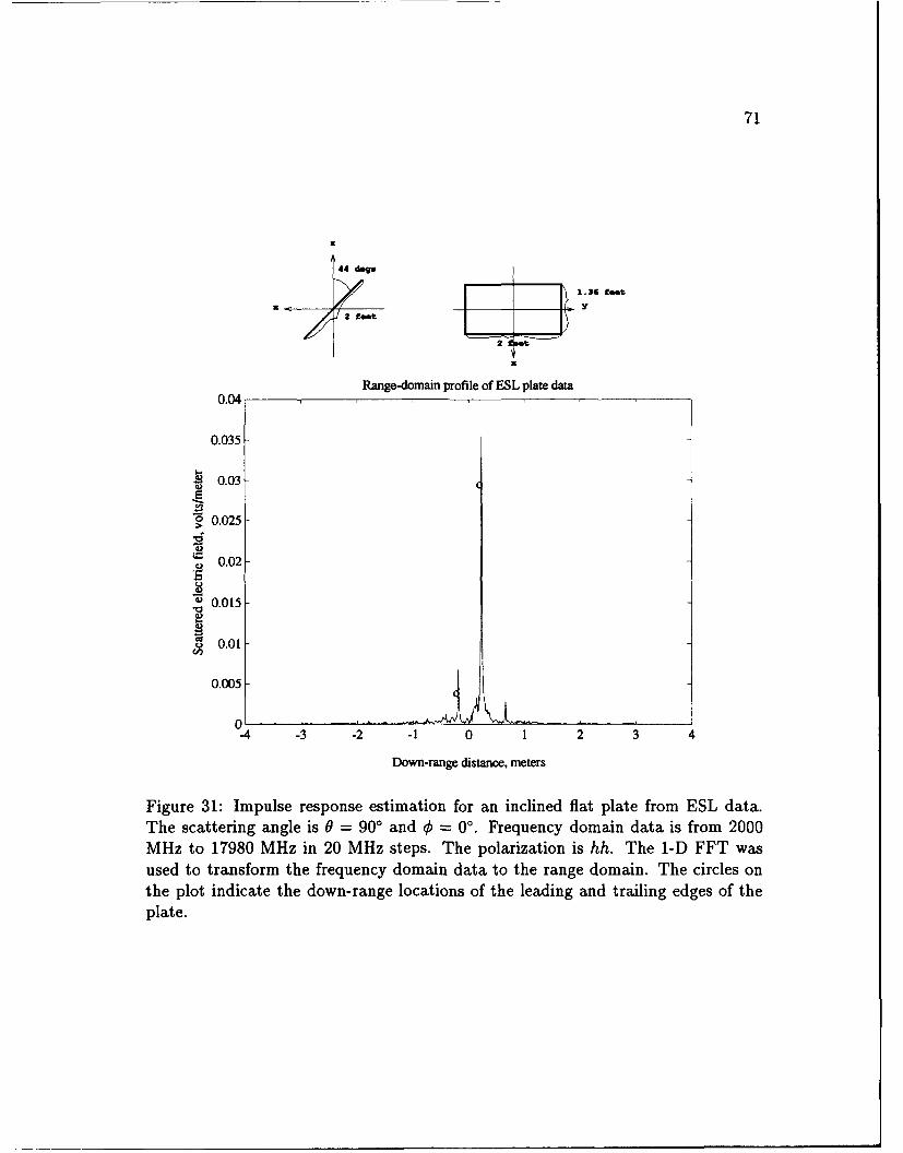
71
Z
44 de"S
1.36 feet
IY
2~ f..t
Range-domain profile of ESL plate data0.04
0.035
0.03
o 0.025
0.02
o 0.015
5 0.01
0.005
-4 -3 -2 -1 0 1 2 3 4
Down-range distance, meters
Figure 31: Impulse response estimation for an inclined flat plate from ESL data.The scattering angle is 0 = 900 and 0 = 0'. Frequency domain data is from 2000MHz to 17980 MHz in 20 MHz steps. The polarization is hh. The 1-D FFT wasused to transform the frequency domain data to the range domain. The circles onthe plot indicate the down-range locations of the leading and trailing edges of theplate.

72
44 "gou
/ 1.36 feet/Y
2~ 1in
It
Range-domain profile of ESL plate data0.04
0.035
4) 0.03
o 0.025
0.02
' 0.015
o 0.01
0.005-
0- --0.8 -0.6 -0.4 -0.2 0 0.2 0.4 0.6 0.8 1
Down-range distance, meters
Figure 32: Impulse response estimation for an inclined flat plate from ESL data.The scattering angle is 0 = 90' and 0 = 00. Frequency domain data is from 2000MHz to 17980 MHz in 20 MHz steps. The polarization is hh. Only the part of theimpulse response which contains the plate data is shown. The 1-D FFT was used totransform the frequency domain data to the range domain. The circles on the plotindicate the down-range locations of the leading and trailing edges of the plate.
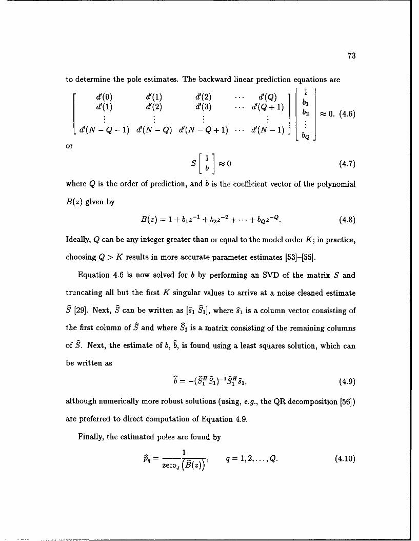
73
to determine the pole estimates. The backward linear prediction equations are
d'(O) d'(1) d'(2) ... d'(Q) 1d'(l) d'(2) d'(3) ... d'(Q 1) bI
6'[ + ) b 0. (4.6)
d'(N - Q - 1) d'(N - Q) d'(N - Q + 1) ... d'(N - 1) bQ _
or
S b 0 (4.7)
where Q is the order of prediction, and b is the coefficient vector of the polynomial
B(z) given by
B(z) = 1 + biz - 1 + b2 z- 2 +... + bQz - Q . (4.8)
Ideally, Q can be any integer greater than or equal to the model order K; in practice,
choosing Q > K results in more accurate parameter estimates [53]-[55].
Equation 4.6 is now solved for b by performing an SVD of the matrix S and
truncating all but the first K singular values to arrive at a noise cleaned estimate
9 [29]. Next, S can be written as ['1 911, where 9, is a column vector consisting of
the first column of S and where $1 is a matrix consisting of the remaining columns
of S. Next, the estimate of b, b, is found using a least squares solution, which can
be written as
b = -( 1' Sx (4.9)
although numerically more robust solutions (using, e.g., the QR decomposition [56])
are preferred to direct computation of Equation 4.9.
Finally, the estimated poles are found by
11 q = 1,2,..., Q. (4.10)zeo W
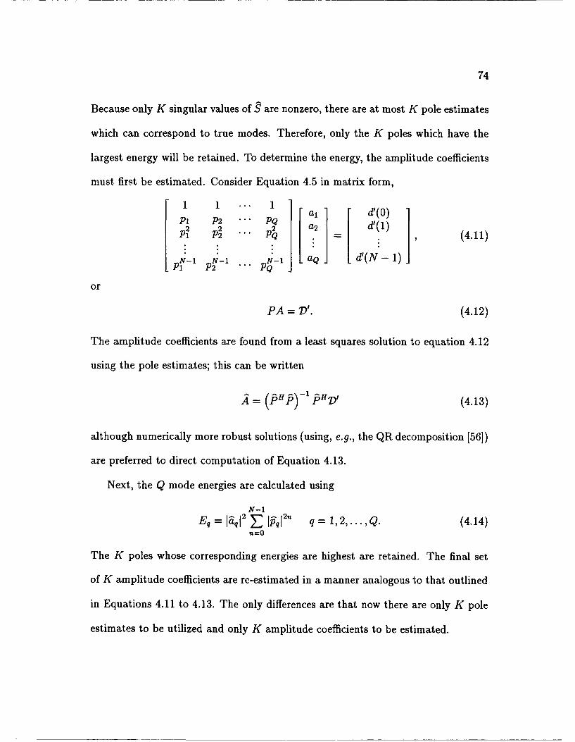
74
Because only K singular values of § are nonzero, there are at most K pole estimates
which can correspond to true modes. Therefore, only the K poles which have the
largest energy will be retained. To determine the energy, the amplitude coefficients
must first be estimated. Consider Equation 4.5 in matrix form,
1 1 1.. 1 d (O)2 22 a2 d'(1)
Pi P2 ".. PQ d'(1) (4.11)
N-1 N-1 N-1 aQ d(N-1)j
or
PA= V. (4.12)
The amplitude coefficients are found from a least squares solution to equation 4.12
using the pole estimates; this can be written
= (PH P) 1 .PHVI (4.13)
although numerically more robust solutions (using, e.g., the QR decomposition [56])
are preferred to direct computation of Equation 4.13.
Next, the Q mode energies are calculated using
N-1
Eq = Iaq12 1 1I&12n q= 1,2,...,Q. (4.14)
The K poles whose corresponding energies are highest are retained. The final set
of K amplitude coefficients are re-estimated in a manner analogous to that outlined
in Equations 4.11 to 4.13. The only differences are that now there are only K pole
estimates to be utilized and only K amplitude coefficients to be estimated.
75
Prony's model is now applied to the radar data of a flat plate obtained at the
ElectroScience Laboratory. In order to make this example more realistic in terms
of radar data, only a limited bandwidth of the data will be used. Frequencies from
8-9 GHz are used, with a frequency step of 20 MHz between samples. The FFT
of this limited bandwidth data is shown in Figure 33. The 'o's in the plot denote
the locations of the leading and trailing edges of the flat plate. From this figure we
see that the edges and multiple bounce phenomena associated with the plate are
unresolvable using the IFFT. Using the SVD-Prony method described above, with
model orders Q, K = 18,4, the impulse response shown in Figure 34 was found from
the original 51 data points.
Figure 34 shows how the SVD-Prony method easily resolved the leading and
trailing edges of the plate along with the multiple bounce phenomena. This ex-
ample demonstrates the utility of parametric techniques such as Prony's model to
superresolve scattering centers on a target.
4.3 Two-Dimensional Techniques
As in 1-D, methods of obtaining range-domain profiles of the target have centered
around the 2-D Fourier Transform. First, the relationship between the frequency
domain and the time domain will be established. The 2-D image of a raaar target
is sometimes called "the reflectivity density function" [57] and is denoted h (x, y).
The radar-target geometry for 2-D imaging purposes is showii in Figure 35. The
uv-coordinates are fixed to the radar while the xy-coordinates are fixed to the target.
The range between the maximum extent of the target and the radar is assumed to
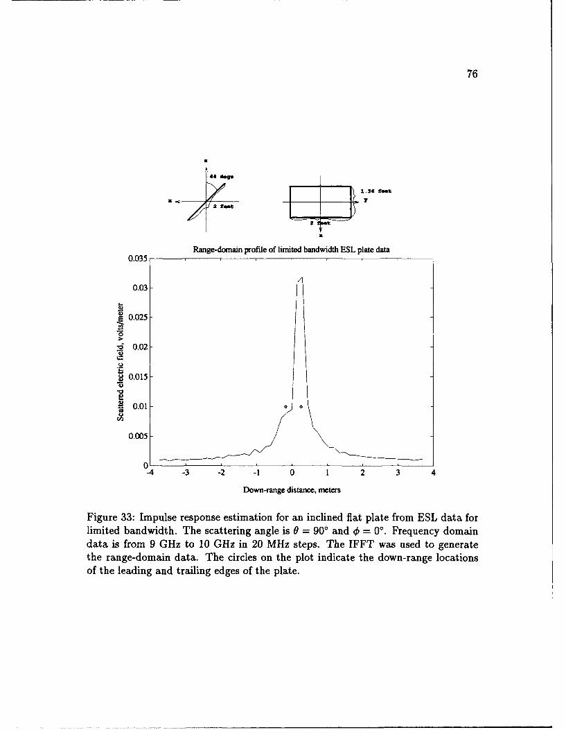
76
A
44 4*9*
1.36 96*t
2 fee"t
Range-domain profile of limited bandwidth ESL plate data0.035
0.03
0.025
_ 0.02
0.015
0.005
0-4 -3 -2 -1 0 1 2 3 4
Down-range distance, meters
Figure 33: Impulse response estimation for an inclined flat plate from ESL data forlimited bandwidth. The scattering angle is 0 = 900 and 4 = 00. Frequency domaindata is from 9 GHz to 10 GHz in 20 MHz steps. The IFFT was used to generatethe range-domain data. The circles on the plot indicate the down-range locationsof the leading and trailing edges of the plate.
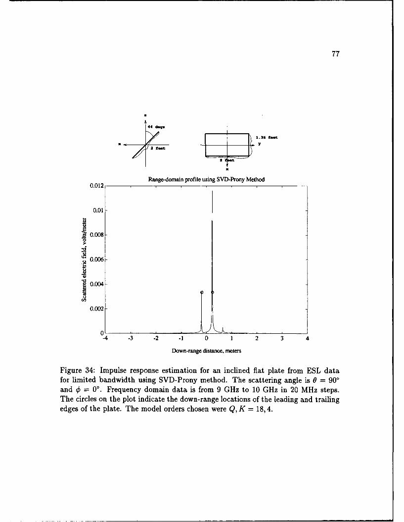
77
44 dg
F _ 1. 36 rest
J2 feet22 gm
Range-domain profile using SVD-Prony Method0.012
0.01
0.008
0.006
S0.004
C'
0.002
0-4 -3 -2 -1 0 1 2 3 4
Down-range distance, meters
Figure 34: Impulse response estimation for an inclined flat plate from ESL datafor limited bandwidth using SVD-Prony method. The scattering angle is 0 = 90'and 0 = 0'. Frequency domain data is from 9 GHz to 10 GHz in 20 MHz steps.The circles on the plot indicate the down-range locations of the leading and trailingedges of the plate. The model orders chosen were Q, K = 18,4.
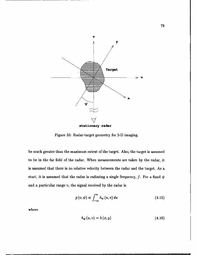
78
V
y
Target
Vstationary radar
Figure 35: Radar-target geometry for 2-D imaging.
be much greater than the maximum extent of the target. Also, the target is assumed
to be in the far field of the radar. When measurements are taken by the radar, it
is assumed that there is no relative velocity between the radar and the target. As a
start, it is assumed that the radar is radiating a single frequency, f. For a fixed I
and a particular range v, the signal received by the radar is
00p (v, O) oc 0 h-0,(u, v)du (4.15)
where
h =(u,v) = h(x,y) (4.16)
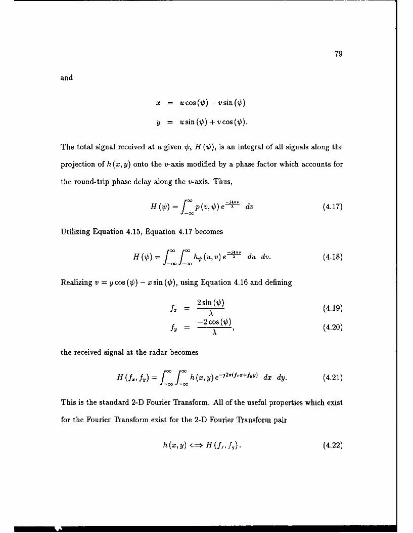
79
and
x = u cos () -vsin (V)
y = u sin (7p) + v cos (V).
The total signal received at a given 0, H (V)), is an integral of all signals along the
projection of h (x, y) onto the v-axis modified by a phase factor which accounts for
the round-trip phase delay along the v-axis. Thus,
H()= p(v,O)e A dv (4.17)
Utilizing Equation 4.15, Equation 4.17 becomes
H (4') = hp (u, v) e du dv. (4.18)
Realizing v = ycos (4) - xsin (4), using Equation 4.16 and defining
= 2 sin ()(4.19)A-2 cos (4)
fy = A2 , (4.20)
the received signal at the radar becomes
H(fx, f) = Ljf00h(x,y)e-i21r(f.+fYY) dx dy. (4.21)
This is the standard 2-D Fourier Transform. All of the useful properties which exist
for the Fourier Transform exist for the 2-D Fourier Transform pair
h (x, y) -= ( ,,). (4.22)
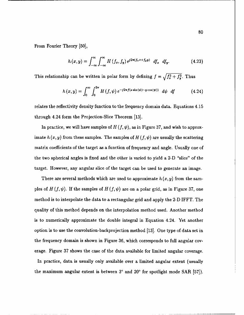
80
From Fourier Theory [501,
h (x, y) H (f, fY) ej alIifz+fyV) df. dfv. (4.23)
This relationship can be written in polar form by defining f = f2 + f2. Thus
h (x, y) = f H (f, 4) e- j 2wf( xsin) -Ic °8( '/)) do df (4.24)
relates the reflectivity density function to the frequency domain data. Equations 4.15
through 4.24 form the Projection-Slice Theorem [13].
In practice, we will have samples of H (f, 4), as in Figure 37, and wish to approx-
imate h (x, y) from these samples. The samples of H (f, 4) are usually the scattering
matrix coefficients of the target as a function of frequency and angle. Usually one of
the two spherical angles is fixed and the other is varied to yield a 2-D "slice" of the
target. However, any angular slice of the target can be used to generate an image.
There are several methods which are used to approximate h (x, y) from the sam-
ples of H (f,,4). If the samples of H (f, 4) are on a polar grid, as in Figure 37, one
method is to interpolate the data to a rectangular grid and apply the 2-D IFFT. The
quality of this method depends on the interpolation method used. Another method
is to numerically approximate the double integral in Equation 4.24. Yet another
option is to use the convolution-backprojection method [13]. One type of data set in
the frequency domain is shown in Figure 36, which corresponds to full angular cov-
erage. Figure 37 shows the case of the data available for limited angular coverage.
In practice, data is usually only available over a limited angular extent (usually
the maximum angular extent is between 30 and 200 for spotlight mode SAR [57]).
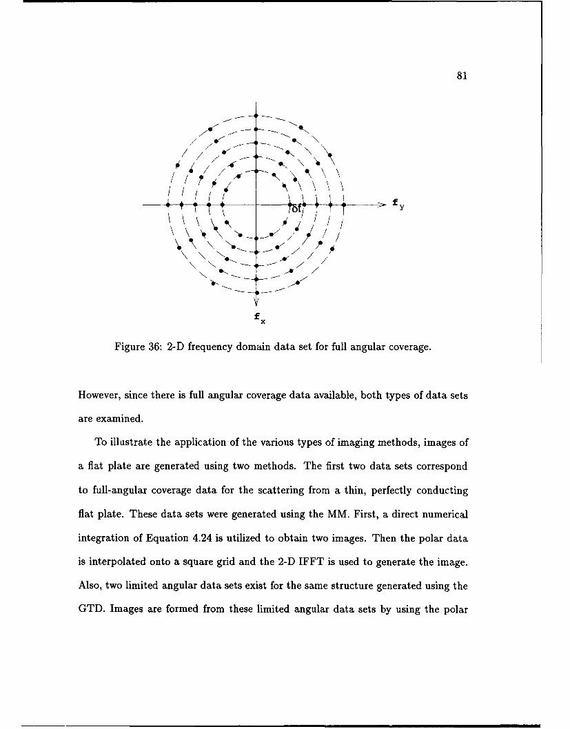
81
II Ap I
I/f / --4
are examined.
/ ,/
K -"
x
Figure 36: 2-D frequency domain data set for full angular coverage.
However, since there is full angular coverage data available, both types of data sets
are examined.
To illustrate the application of the various types of imaging methods, images of
a flat plate are generated using two methods. The first two data sets correspond
to full-angular coverage data for the scattering from a thin, perfectly conducting
flat plate. These data sets were generated using the MM. First, a direct numerical
integration of Equation 4.24 is utilized to obtain two images. Then the polar data
is interpolated onto a square grid and the 2-D IFFT is used to generate the image.
Also, two limited angular data sets exist for the same structure generated using the
GTD. Images are formed from these limited angular data sets by using the polar
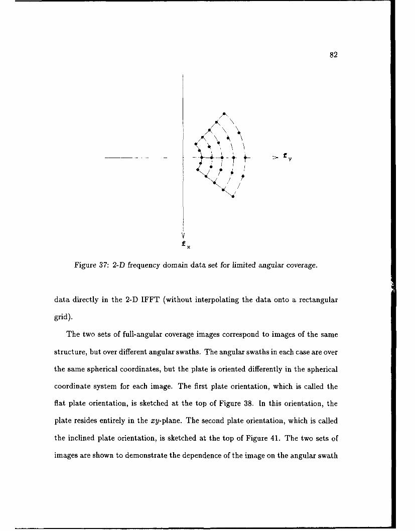
82
/
f x
Figure 37: 2-D frequency domain data set for limited angular coverage.
data directly in the 2-D IFFT (without interpolating the data onto a rectangular
grid).
The two sets of full-angular coverage images correspond to images of the same
structure, but over different angular swaths. The angular swaths in each case are over
the same spherical coordinates, but the plate is oriented differently in the spherical
coordinate system for each image. The first plate orientation, which is called the
flat plate orientation, is sketched at the top of Figure 38. In this orientation, the
plate resides entirely in the xy-plane. The second plate orientation, which is called
the inclined plate orientation, is sketched at the top of Figure 41. The two sets of
images are shown to demonstrate the dependence of the image on the angular swath
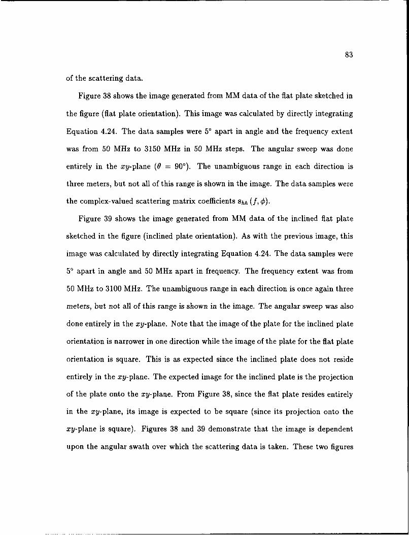
83
of the scattering data.
Figure 38 shows the image generated from MM data of the flat plate sketched in
the figure (flat plate orientation). This image was calculated by directly integrating
Equation 4.24. The data samples were 50 apart in angle and the frequency extent
was from 50 MHz to 3150 MHz in 50 MHz steps. The angular sweep was done
entirely in the xy-plane (0 = 900). The unambiguous range in each direction is
three meters, but not all of this range is shown in the image. The data samples were
the complex-valued scattering matrix coefficients Shh (f, ).
Figure 39 shows the image generated from MM data of the inclined flat plate
sketched in the figure (inclined plate orientation). As with the previous image, this
image was calculated by directly integrating Equation 4.24. The data samples were
50 apart in angle and 50 MHz apart in frequency. The frequency extent was from
50 MHz to 3100 MHz. The unambiguous range in each direction is once again three
meters, but not all of this range is shown in the image. The angular sweep was also
done entirely in the xy-plane. Note that the image of the plate for the inclined plate
orientation is narrower in one direction while the image of the plate for the flat plate
orientation is square. This is as expected since the inclined plate does not reside
entirely in the xy-plane. The expected image for the inclined plate is the projection
of the plate onto the xy-plane. From Figure 38, since the flat plate resides entirely
in the xy-plane, its image is expected to be square (since its projection onto the
xy-plane is square). Figures 38 and 39 demonstrate that the image is dependent
upon the angular swath over which the scattering data is taken. These two figures
84
0.5 motors
0. 5 meters
-- y
xPlate resides entirely in xy-plane
Plate is 0.5 meters square
Figure 38: Image of a plate, in the flat plate orientation, generated by direct numer-ical integration of Equation 4.24 for full angular coverage data (hh-polarization).
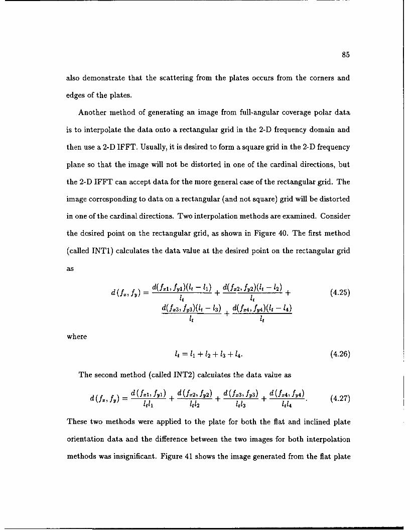
85
also demonstrate that the scattering from the plates occurs from the corners and
edges of the plates.
Another method of generating an image from full-angular coverage polar data
is to interpolate the data onto a rectangular grid in the 2-D frequency domain and
then use a 2-D IFFT. Usually, it is desired to form a square grid in the 2-D frequency
plane so that the image will not be distorted in one of the cardinal directions, but
the 2-D IFFT can accept data for the more general case of the rectangular grid. The
image corresponding to data on a rectangular (and not square) grid will be distorted
in one of the cardinal directions. Two interpolation methods are examined. Consider
the desired point on the rectangular grid, as shown in Figure 40. The first method
(called INT1) calculates the data value at the desired point on the rectangular grid
as
d (f f_) = d(f.1 , fyi)(lt - l1) + d(f. 2, fy2)(It - 12) + (4.25)it it
d(f. 3, fy3)(it - 13) + d(f.4 , fV4)(lt - 14)
it it
where
It = ll + 12 + 13 + 14. (4.26)
The second method (called INT2) calculates the data value as
d(f,,f)- d(f.1 , fyl) + d(f 2, fv 2) + dU.3, f 3) + d(f.4,f 4) (4.27)ltll 4 l12 41l3 ltl4
These two methods were applied to the plate for both the flat and inclined plate
orientation data and the difference between the two images for both interpolation
methods was insignificant. Figure 41 shows the image generated from the flat plate
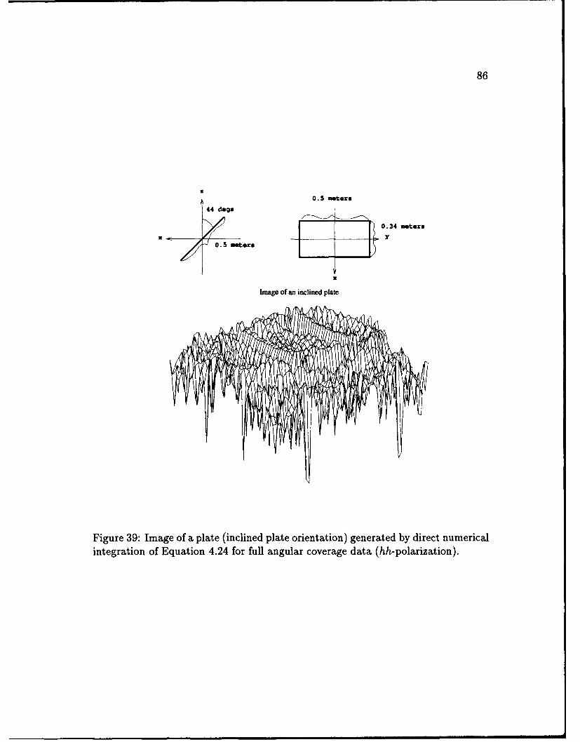
86
z
0. 5 maters
44 dogs
0.34 meters__ y
J 0.5 'meters
Image of an inclined plate
Figure 39: Image of a plate (inclined plate orientation) generated by direct numericalintegration of Equation 4.24 for full angular coverage data (hh-polarization).
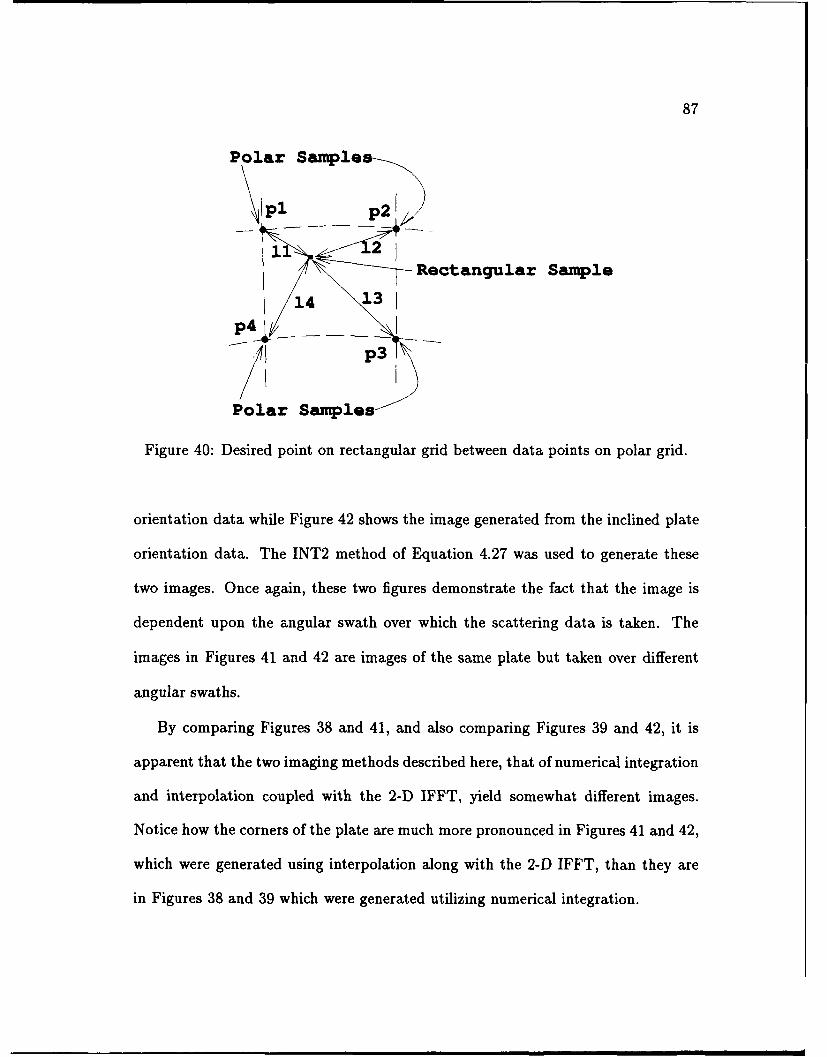
87
Polar Samples-
p1 p2l
11 Rectangular Sample
14 13~
I p3
Polar Samples
Figure 40: Desired point on rectangular grid between data points on polar grid.
orientation data while Figure 42 shows the image generated from the inclined plate
orientation data. The INT2 method of Equation 4.27 was used to generate these
two images. Once again, these two figures demonstrate the fact that the image is
dependent upon the angular swath over which the scattering data is taken. The
images in Figures 41 and 42 are images of the same plate but taken over different
angular swaths.
By comparing Figures 38 and 41, and also comparing Figures 39 and 42, it is
apparent that the two imaging methods described here, that of numerical integration
and interpolation coupled with the 2-D IFFT, yield somewhat different images.
Notice how the corners of the plate are much more pronounced in Figures 41 and 42,
which were generated using interpolation along with the 2-D IFFT, than they are
in Figures 38 and 39 which were generated utilizing numerical integration.
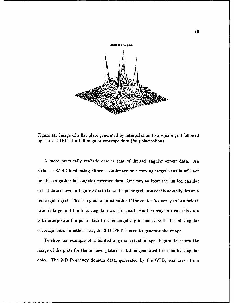
88
Imae of a flt plate
Figure 41: Image of a flat plate generated by interpolation to a square grid followedby the 2-D IFFT for full angular coverage data (hh-polarization).
A more practically realistic case is that of limited angular extent data. An
airborne SAR illuminating either a stationary or a moving target usually will not
be able to gather full angular coverage data. One way to treat the limited angular
extent data shown in Figure 37 is to treat the polar grid data as if it actually lies on a
rectangular grid. This is a good approximation if the center frequency to bandwidth
ratio is large and the total angular swath is small. Another way to treat this data
is to interpolate the polar data to a rectangular grid just as with the full angular
coverage data. In either case, the 2-D IFFT is used to generate the image.
To show an example of a limited angular extent image, Figure 43 shows the
image of the plate for the inclined plate orientation generated from limited angular
data. The 2-D frequency domain data, generated by the GTD, was taken from
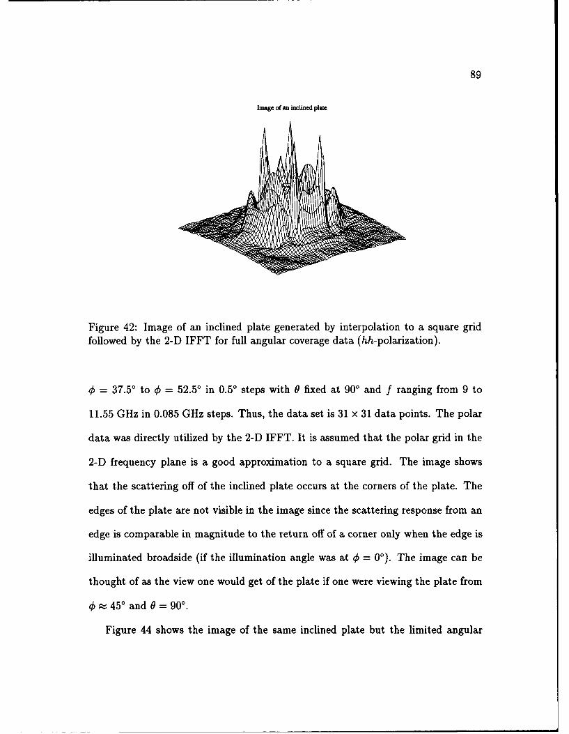
89
Image of an inclined plate
Figure 42: Image of an inclined plate generated by interpolation to a square gridfollowed by the 2-D IFFT for full angular coverage data (hh-polarization).
0 = 37.5' to 4 = 52.50 in 0.5' steps with 0 fixed at 900 and f ranging from 9 to
11.55 GHz in 0.085 GHz steps. Thus, the data set is 31 x 31 data points. The polar
data was directly utilized by the 2-D IFFT. It is assumed that the polar grid in the
2-D frequency plane is a good approximation to a square grid. The image shows
that the scattering off of the inclined plate occurs at the corners of the plate. The
edges of the plate are not visible in the image since the scattering response from an
edge is comparable in magnitude to the return off of a corner only when the edge is
illuminated broadside (if the illumination angle was at 4 = 00). The image can be
thought of as the view one would get of the plate if one were viewing the plate from
4): 450 and 0 = 900.
Figure 44 shows the image of the same inclined plate but the limited angular
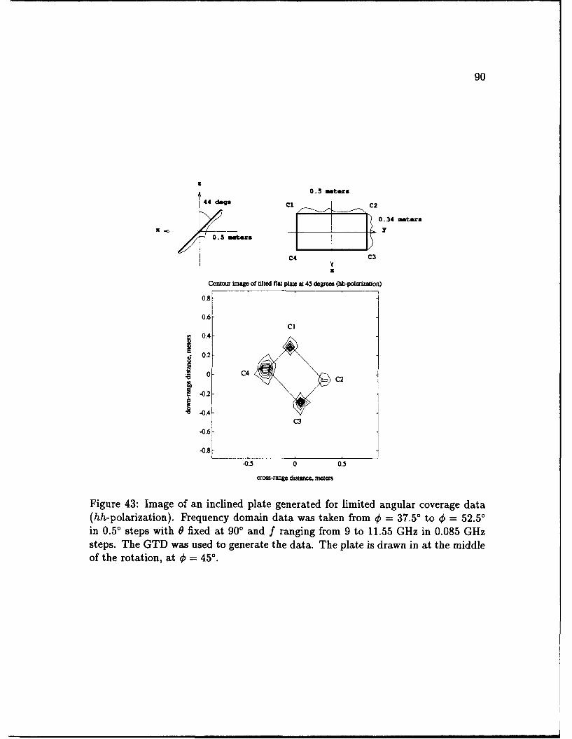
90
U!
0. 5 motors
44 ogs Cl C2
/ 0.34 moters
0.5 moers
C4 C3
x
Contour image of tilted flat plate at 45 degrees (hh-polmization)
0.8
0.6C1
0.4
0.2-
• 0 - C 4 CC24
-0.2
S-0.4C3
-0.6
-0.8-0.5 0 0.5
crs-range distace, meters
Figure 43: Image of an inclined plate generated for limited angular coverage data(hh-polarization). Frequency domain data was taken from 0 = 37.50 to 0 = 52.50in 0.50 steps with 0 fixed at 900 and f ranging from 9 to 11.55 GHz in 0.085 GHzsteps. The GTD was used to generate the data. The plate is drawn in at the middleof the rotation, at 4 = 45 .
91
data is taken over a different angular sector. The frequency domain data was taken
from 4 = -7.5' to q$ = 7.5' in 0.50 steps with 0 fixed at 90' and f ranging from 9
to 11.55 GHz in 0.085 GHz steps. Again, the GTD was used to generate the data
and the data set consists of 31 x 31 data points. The polar data was directly input
into the 2-D IFFT. This image shows how the edges of the plate appear in images
when the viewing angles include those broadside to the edge (0 = 0' in this case).
For this plate, the hh-polarization response from the front edge is much larger than
the response from the rear edge (the front edge is the one at x = 0.173 meters).
In the above examples the angular and frequency spacing was chosen so that
the data points in the 2-D frequency plane were roughly evenly spaced. Also, the
GTD was used for the limited angular extent examples so that the data would be
at frequencies around 10 GHz, which allows the spacing at the lowest frequency to
be no less than 0.78 times the spacing at the highest frequency. The MM could not
produce data at frequencies this high due to CPU/memory constraints.
4.4 Summary
This chapter was a background signal processing chapter which was needed to intro-
duce 1-D and 2-D signal processing techniques. Non-parametric techniques such as
the 1-D and 2-D IFFTs were introduced and examples were shown on how these tech-
niques produce a down-range profile and an image of a target, respectively. The 1-D
TLS-Prony Technique was described, which is a 1-D parametric signal processing
technique. Prony's model (in 1-D) was introduced, which is the 1-D damped expo-
nential model utilized by the 1-D TLS-Prony Technique. The estimation algorithm
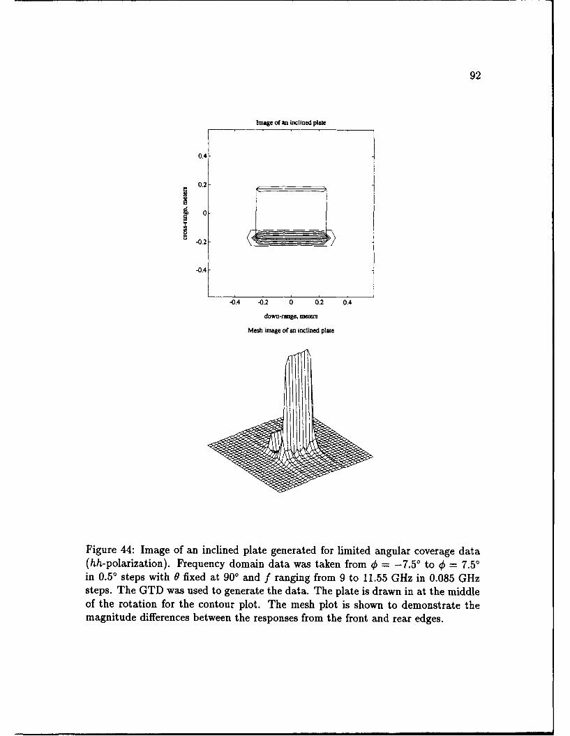
92
Image of an inclined plate
0.4
0.2
e 0
-0.4
-0.4 -0.2 0 0.2 0.4
down-range, meters
Mesh image of an inclined plate
Figure 44: Image of an inclined plate generated for limited angular coverage data(hh-polarization). Frequency domain data was taken from 0 = -7.5' to 0 = 7.5'in 0.50 steps with 0 fixed at 900 and f ranging from 9 to 11.55 GHz in 0.085 GHzsteps. The GTD was used to generate the data. The plate is drawn in at the middleof the rotation for the contour plot. The mesh plot is shown to demonstrate themagnitude differences between the responses from the front and rear edges.

93
utilized by this technique was described, and examples were shown on its abilities.
Several 2-D IFFT based image generation techniques were described such as numer-
ical integration, interpolation to a rectangular grid and convolution-backprojection.
Images generated by the various techniques were shown and issues such as angular
swath orientation and 2-D frequency and angular bandwidths were discussed.
CHAPTER V
The Two-Dimensional TLS-Prony Technique
5.1 Introduction
This chapter presents a new technique to estimate two-dimensional (2-D) exponen-
tials and their associated amplitude coefficients from a 2-D data set. It is called the
2-D TLS-Prony Technique. First, the model and estimation algorithm are devel-
oped for a basic 2-D data set. This data set could correspond, for example, to the
data set collected by a SAR for a single transmit and receive polarization. The algo-
rithm is then extended to utilize multiple data sets which can correspond to multiple
transmit and receive polarization data. This is designated the full-polarization case.
5.2 Basic Technique Description
5.2.1 Background and Introduction
The 2-D TLS-Prony Technique is a parametric technique for the estimation of 2-D
exponentials and their associated amplitude coefficients. The model used for the
data is a 2-D extension of the 1-D Prony Model in Equation 4.5. Prony's method
coupled with a total least squares (TLS) technique in 1-D has been successfully
used to estimate frequencies in the presence of noise [29] as shown in Chapter IV.
With the 2-D TLS-Prony Technique, 2-D exponentias and amplitude coefficients
94
95
are estimated by a two-step method using a 1-D TLS-based Prony model and esti-
mation technique in each step. This technique is capable of estimating 2-D damped
exponentials.
A related method, developed by Hua [28], estimates 2-D frequencies. In Hua's
method, two estimation steps are performed to separately estimate the x-components
and y-components of the 2-D frequencies. Then, a matching step is performed to
find the correct x-component and y-component frequency pairings. The 2-D TLS-
Prony Technique is similar to Hua's in some respects, but different in others. With
the 2-D TLS-Prony Technique, the x-components of the exponentials are estimated
first. Then amplitude coefficients corresponding to each x-component exponential
are estimated and these estimates are used to estimate a set of y-component expo-
nentials. In this way the requirement of a matching step is avoided. This algorithm
is computationally less expensive than Hua's method, and more amenable to parallel
implementation. A second algorithm is also presented in which the first algorithm
is used twice, first to estimate x then y-component exponentials and then y then
x-component exponentials. The second algorithm does require matching, but the
computational load is still smaller than the one in [28]. This second algorithm gives
more accurate parameter estimates than the first algorithm.
5.2.2 Data Model
The given noisy 2-D data is assumed to have the form
d'(m, n) = d(m, n) + w(m, n), (5.1)
96
where m = 0, 1,... M - 1 and n = 0, 1,... N - 1 and w(m, n) is 2-D noise sequence.
The first index of d(m, n) is referred to as the x-component, and the second index as
the y-component. The x-component is analogous to the frequency component and
the y-component is analogous to the angular component in the 2-D frequency plane.
However, the data which is used in this algorithm is assumed to lie on a rectangular
grid on the 2-D frequency plane, not a polar grid as is associated with data on the
2-D freqency plane which is collected by SARs. Tlus, if the initial data lies on a
polar grid, it should be interpolated onto a rectangular grid before it is used by the
2-D TLS-Prony Technique. This issue is investigated in Chapter VI.
The noiseless data is assumed to fit the 2-D damped exponential model
K Lkd(m, n) = (5.2)
k=1 1= 1
where
P=k = kth x-pole, x-component of 2-D exponential
P k, = k, lth y-pole, y-component of 2-D exponential
ak,z = k, lth amplitude coefficient
K = number of x-poles
= number of y-poles corresponding to the kth x-pole.
The 2-D Z-transform is defined for the model in equation 5.2 as
k(u,v) ak, (5.3)k 1 1=1 ( PXk zu) (1 _ PYkIZV)
where z,, = ei " and z, = el [58]. Thus, each 2-D frequency is determined by the
intersection of its x and y-pole locations.
97
Given noisy data d'(m,n), m = 0,1,...M - 1 and n = 0,1,...N - 1, the
parameters in the model 5.2 must be estimated. Below two TLS-Prony based al-
gorithms for estimating these parameters are presented, called Algorithm One and
Algorithm Two.
5.2.3 Estimation Algorithms
Algorithm One
Algorithm One consists of four steps. The x-poles, {pzK 1, are first estimated using}k=,arfisesiteusn
a TLS-Prony algorithm. Second, a set of amplitude coefficients corresponding to
these x-pole estimates are computed. The amplitude coefficients are themselves used" K,LLk
in a set of second TLS-Prony estimates to obtain the y-pole estimates, {p~k'lk,=1,
which is the third step. Finally, a least squares technique is used to estimate the
amplitude coefficients fak,1}Lk~x. These steps are detailed below and summarized in
Table 5.
Step 1: Estimation of the x-poles. The first step in the parameter estimation
problem is to estimate the x-poles, { Kpk=,. A matrix composed of the noisy data,
{d'(mn) }1, , is defined as
d'(0, 0) d'(1, 0) ... dl(M - 1,0)
D' d'(0, 1) d'(1, 1) ... d'(i- 1, 1) (5.4)
d'(O,N- 1) d'(1,N-1) d'(M- 1,N- 1)
Moving across a row in D' is considered moving in the x-direction (frequency, or
down-range) while moving down a column is considered moving in the y-direction
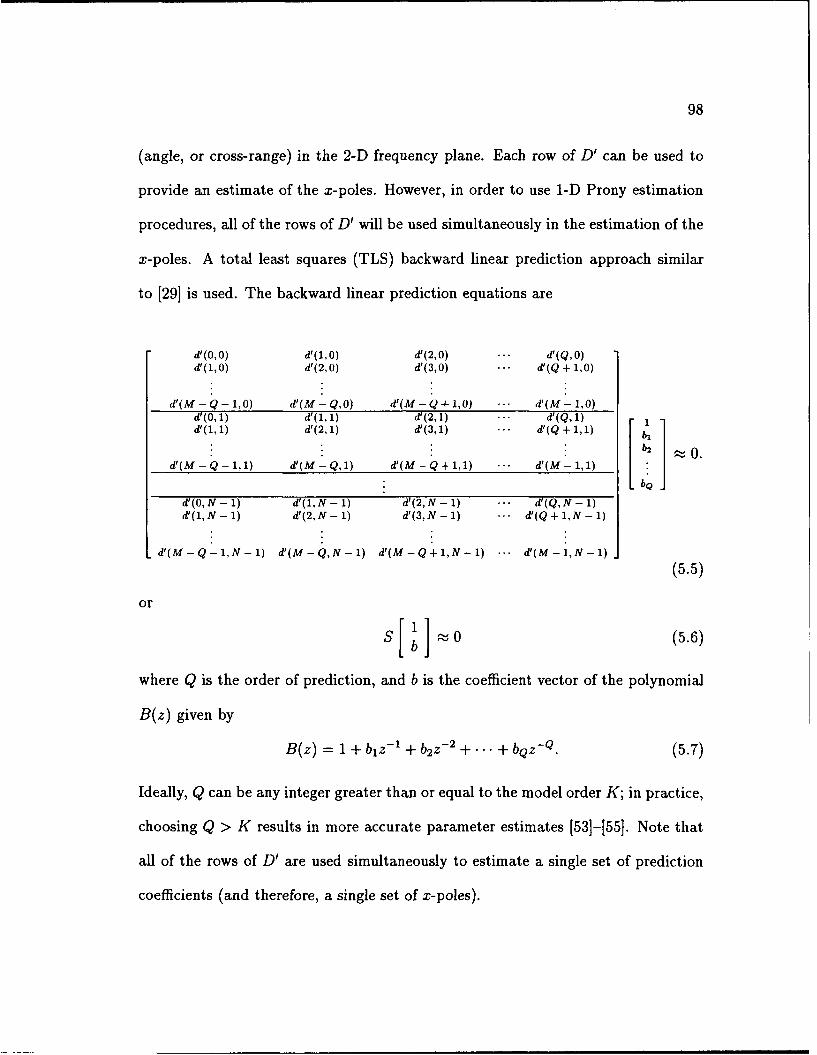
98
(angle, or cross-range) in the 2-D frequency plane. Each row of D' can be used to
provide an estimate of the x-poles. However, in order to use 1-D Prony estimation
procedures, all of the rows of D' will be used simultaneously in the estimation of the
x-poles. A total least squares (TLS) backward linear prediction approach similar
to [29] is used. The backward linear prediction equations are
d'(0,0) d'(1,0) d'(2,0) ... d'(Q,0)d'(1,0) d'(2, 0) d'(3,0) ... d'(Q + 1,0)
d'(M- Q- 1,0) d'(M- Q,0) d'(M- Q + 1,0) ... d'(M- 1,0)d'(0, 1) d'(1, 1) d'(2, 1) ... d'(Q, 1)1
d'(1, 1) d'(2, 1) d'(3, 1) ... d'(Q + 1,1) bi
b2 -0.
d'(M-Q-1,1) d'(M-Q, 1) d'(M-Q+1,1) ... d'(M - 1,1) [bQJ
d'(0, N - 1) d'(1, N - 1) d'(2, N - 1) ... d'(Q, N - 1)d'(1,N -1) d'(2,N -1) d'(3,N- 1) ... d'(Q + 1,N -1)
'(M-Q-1,N-1) d'(M-Q,N-1) d'(M-Q+1,N-1) ... d'(M-1,N-1)
(5.5)
or
s b 0 (5.6)
where Q is the order of prediction, and b is the coefficient vector of the polynomial
B(z) given by
B(z) = 1 + b1z - 1 + b2 z- 2 +... + bQz - Q . (5.7)
Ideally, Q can be any integer greater than or equal to the model order K; in practice,
choosing Q > K results in more accurate parameter estimates [531-[55]. Note that
all of the rows of D' are used simultaneously to estimate a single set of prediction
coefficients (and therefore, a single set of x-poles).
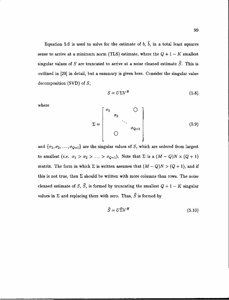
99
Equation 5.6 is used to solve for the estimate of b, b, in a total least squares
sense to arrive at a minimum norm (TLS) estimate, where the Q + 1 - K smallest
singular values of S are truncated to arrive at a noise cleaned estimate S. This is
outlined in [291 in detail, but a summary is given here. Consider the singular value
decomposition (SVD) of S,
S = UVH (5.8)
where
U2
E =(5.9)UQ+1
0
and {al, 0 2 ,.. , oQ+l} are the singular values of S, which are ordered from largest
to smallest (i.e. al >a 2 > ... > aQ+1). Note that E is a (M - Q)N x (Q + 1)
matrix. The form in which E is written assumes that (M - Q)N > (Q + 1), and if
this is not true, then E should be written with more columns than rows. The noise
cleaned estimate of S, S, is formed by truncating the smallest Q + 1 - K singular
values in E and replacing them with zero. Thus, S is formed by
S = U2VH (5.10)
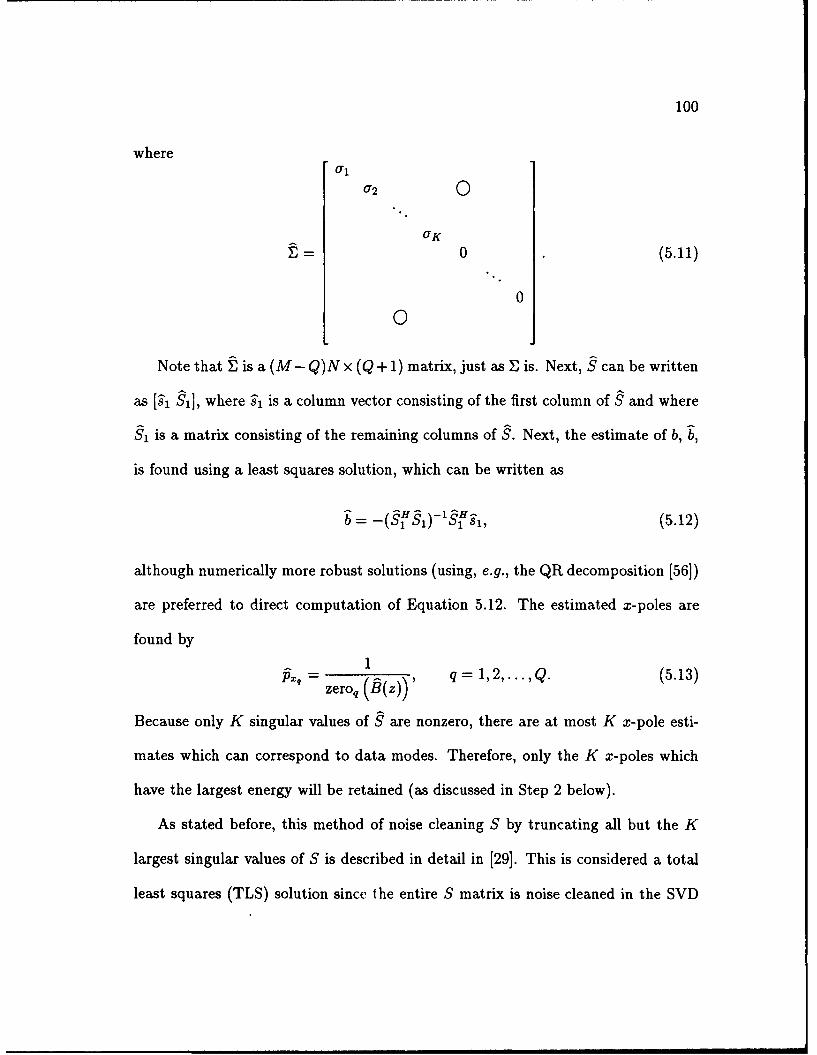
100
where11
U2 0
UfK=0 .(5.11)
00
Note that E is a (M - Q)N x (Q + 1) matrix, just as E is. Next, S can be written
as [ ', S1], where '1 is a column vector consisting of the first column of S and where
$1 is a matrix consisting of the remaining columns of S. Next, the estimate of b, b,
is found using a least squares solution, which can be written as
b = -(S 1 $1)-s1 s, (5.12)
although numerically more robust solutions (using, e.g., the QR decomposition [56])
are preferred to direct computation of Equation 5.12. The estimated x-poles are
found by
1x= , q = 1,2,..., Q. (5.13)
zeroq (F3(Z))
Because only K singular values of S are nonzero, there are at most K x-pole esti-
mates which can correspond to data modes. Therefore, only the K x-poles which
have the largest energy will be retained (as discussed in Step 2 below).
As stated before, this method of noise cleaning S by truncating all but the K
largest singular values of S is described in detail in [29]. This is considered a total
least squares (TLS) solution since the entire S matrix is noise cleaned in the SVD
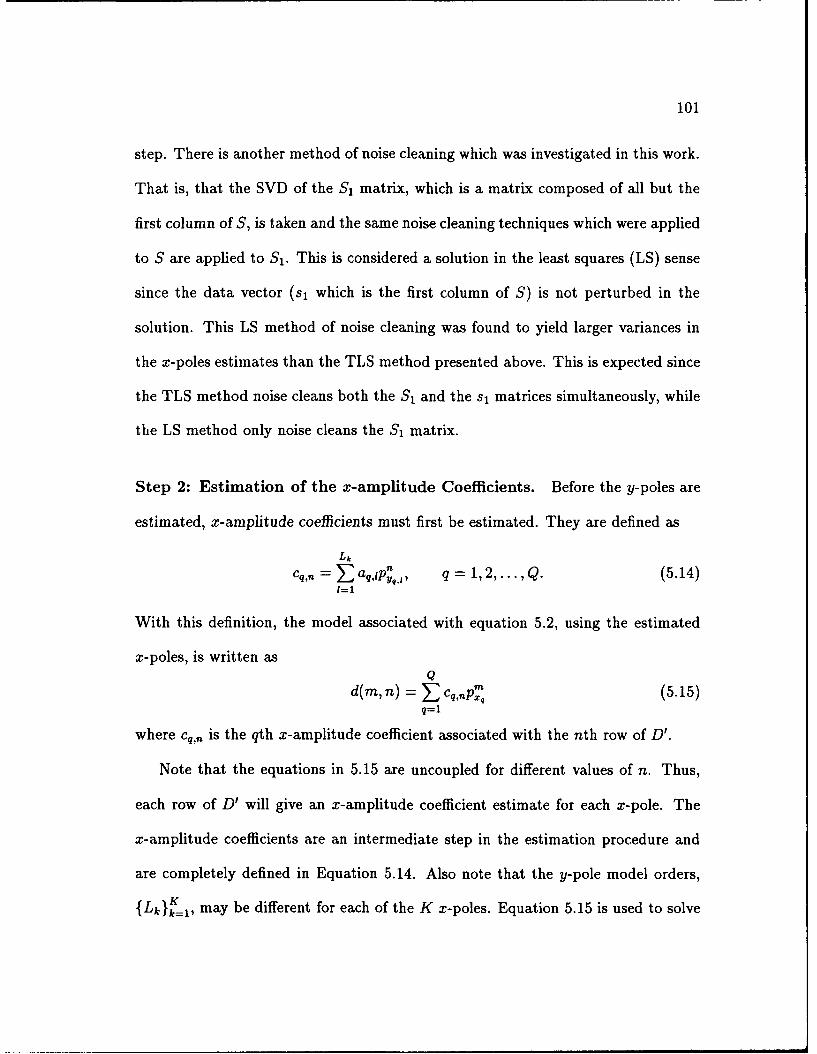
101
step. There is another method of noise cleaning which was investigated in this work.
That is, that the SVD of the S1 matrix, which is a matrix composed of all but the
first column of S, is taken and the same noise cleaning techniques which were applied
to S are applied to S1. This is considered a solution in the least squares (LS) sense
since the data vector (s, which is the first column of S) is not perturbed in the
solution. This LS method of noise cleaning was found to yield larger variances in
the x-poles estimates than the TLS method presented above. This is expected since
the TLS method noise cleans both the S and the S, matrices simultaneously, while
the LS method only noise cleans the S matrix.
Step 2: Estimation of the x-amplitude Coefficients. Before the y-poles are
estimated, x-amplitude coefficients must first be estimated. They are defined as
Lk
Cq,n a aq,P, q = 1,2,.. .,Q. (5.14)/=1
With this definition, the model associated with equation 5.2, using the estimated
x-poles, is written asQ
d(m,n) = _Cq,npx (5.15)q=1
where Cq,n is the qth x-amplitude coefficient associated with the nth row of D'.
Note that the equations in 5.15 are uncoupled for different values of n. Thus,
each row of D' will give an x-amplitude coefficient estimate for each x-pole. The
x-amplitude coefficients are an intermediate step in the estimation procedure and
are completely defined in Equation 5.14. Also note that the y-pole model orders,
Lkk=, may be different for each of the K x-poles. Equation 5.15 is used to solve
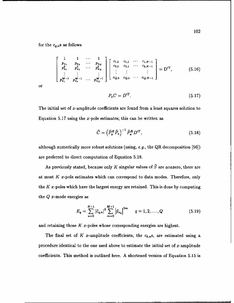
102
for the cq,,,s as follows
1 1 ... 1
PX, PXe PZQ l, C el,1 ... Cl,N 1
21 2 ... 2 C2,0 C2, 1 . C2,N1 IPZ, P " PPzq cX0Q 1.. 2N1 =D 'w (5.16)
M-1 M-1 ... M-1 CQ,O CQ,1 ... CQ,N-1 JP~, PX2 -X
or
P C = DT. (5.17)
The initial set of x-amplitude coefficients are found from a least squares solution to
Equation 5.17 using the x-pole estimates; this can be written as
= (PH P 4 .,DI T , (5.18)
although numerically more robust solutions (using, e.g., the QR decomposition [56])
are preferred to direct computation of Equation 5.18.
As previously stated, because only K singular values of S are nonzero, there are
at most K x-pole estimates which can correspond to data modes. Therefore, only
the K x-poles which have the largest energy are retained. This is done by computing
the Q x-mode energies as
N-1 M-1
Eq = ^ I 2 q l,2,...,Q (5.19)n=O m=O
and retaining those K x-poles whose corresponding energies are highest.
The final set of K x-amplitude coefficients, the ck,ns, are estimated using a
procedure identical to the one used above to estimate the initial set of x-amplitude
coefficients. This method is outlined here. A shortened version of Equation 5.15 is
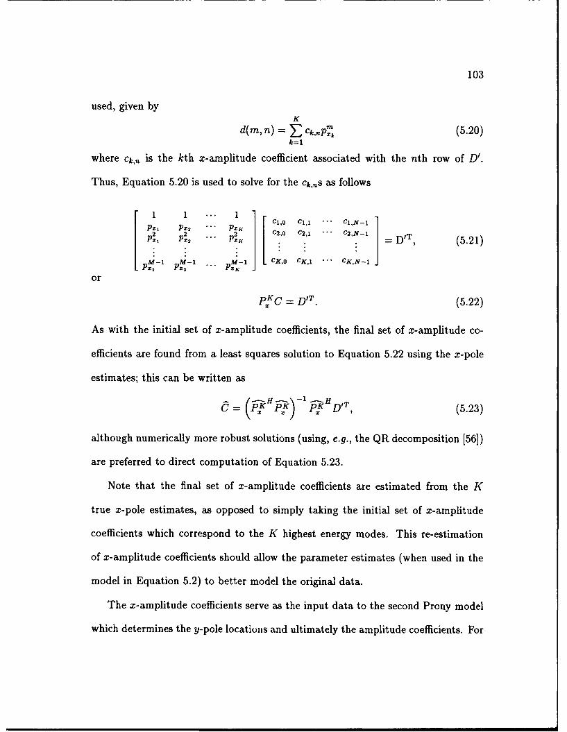
103
used, given byK
d(m, n) = CknP, (5.20)k=1
where ck,n is the kth x-amplitude coefficient associated with the nth row of D'.
Thus, Equation 5.20 is used to solve for the ck,ns as follows
1 1 ... 1
p2 2 ". P2 C2,0 C2 , 1 "'" C2,N-1 I DT, (5.21)p1 P2 2 P2K [ (5.21)~
M -1 M-1 M-1 CK,O CK ...LP2 , PX 2 Pz -
or
pg 0 = DIT. (5.22)
As with the initial set of x-amplitude coefficients, the final set of x-amplitude co-
efficients are found from a least squares solution to Equation 5.22 using the x-pole
estimates; this can be written as
o = (2 HD 'T, (5.23)
although numerically more robust solutions (using, e.g., the QR decomposition [56])
are preferred to direct computation of Equation 5.23.
Note that the final set of x-amplitude coefficients are estimated from the K
true x-pole estimates, as opposed to simply taking the initial set of x-amplitude
coefficients which correspond to the K highest energy modes. This re-estimation
of x-amplitude coefficients should allow the parameter estimates (when used in the
model in Equation 5.2) to better model the original data.
The x-amplitude coefficients serve as the input data to the second Prony model
which determines the y-pole locations and ultimately the amplitude coefficients. For
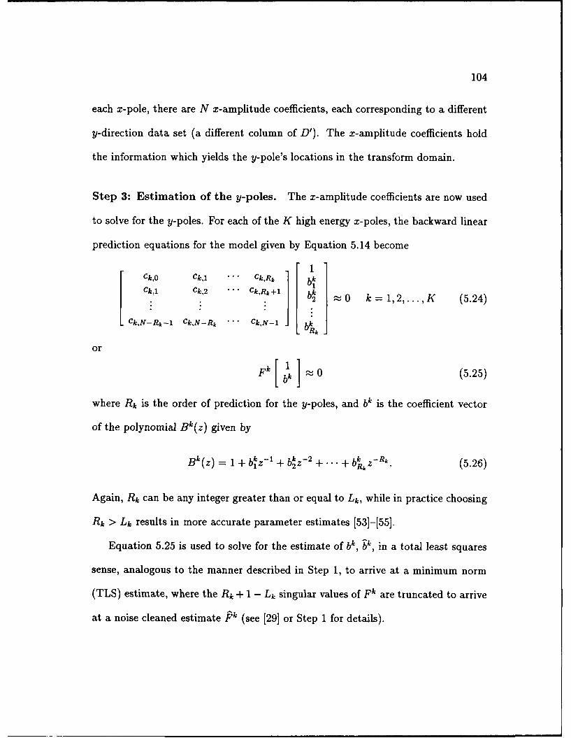
104
each x-pole, there are N x-amplitude coefficients, each corresponding to a different
y-direction data set (a different column of D'). The x-amplitude coefficients hold
the information which yields the y-pole's locations in the transform domain.
Step 3: Estimation of the y-poles. The x-amplitude coefficients are now used
to solve for the y-poles. For each of the K high energy x-poles, the backward linear
prediction equations for the model given by Equation 5.14 become
1Ck,O Ck,1 ... CkRk bkCkl Ck- "'" CR b ,0 k =1,2,..., K (5.24)
Ck,N-Rk-1 Ck,N-Rk .. Ck,N_ 1 .bk.
L Rk -
or
F k k -(5.25)
where Rk is the order of prediction for the y-poles, and bk is the coefficient vector
of the polynomial Bk(z) given by
Bk(z) = 1 + bz - + bkz - 2 ... + b kz - Rk. (5.26)
Again, Rk can be any integer greater than or equal to Lk, while in practice choosing
Rk > Lk results in more accurate parameter estimates [53]-[55].
Equation 5.25 is used to solve for the estimate of bk, bk, in a total least squares
sense, analogous to the manner described in Step 1, to arrive at a minimum norm
(TLS) estimate, where the Rk + 1 - Lk singular values of F' are truncated to arrive
at a noise cleaned estimate Pk (see [29] or Step 1 for details).
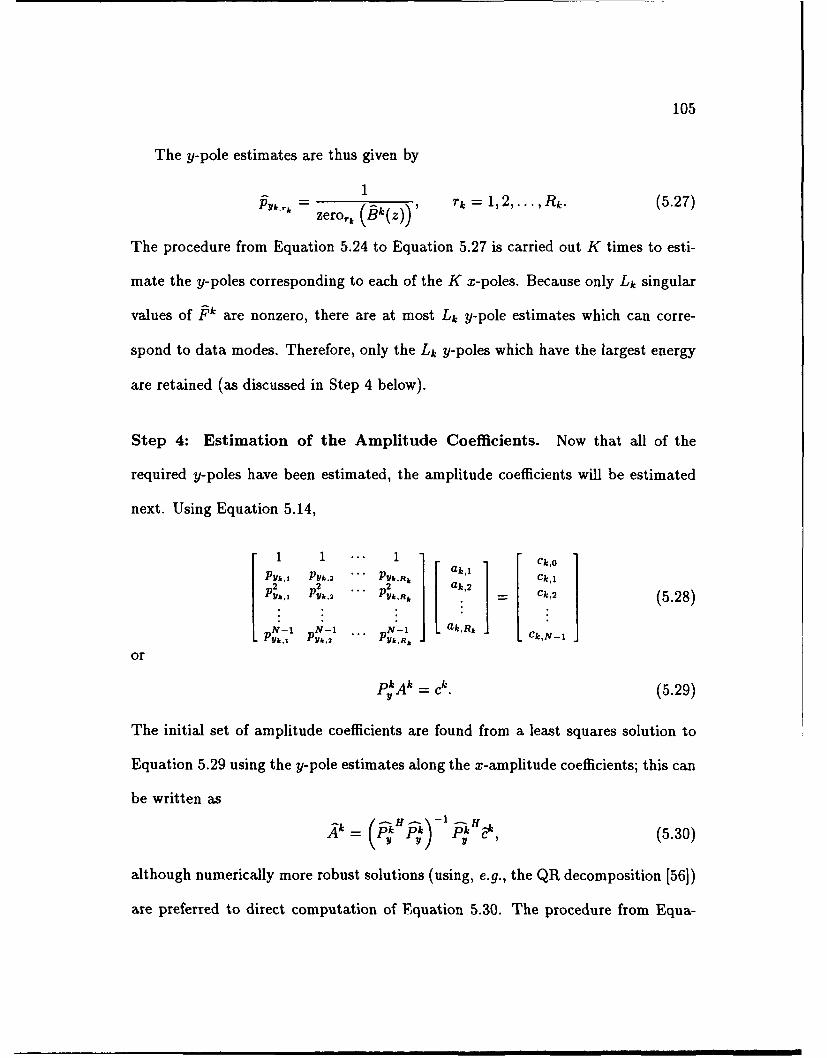
105
The y-pole estimates are thus given by
1P zerok (Ok(z))' rk = 1, 2,..., Rk. (5.27)
The procedure from Equation 5.24 to Equation 5.27 is carried out K times to esti-
mate the y-poles corresponding to each of the K x-poles. Because only Lk singular
values of Pk are nonzero, there are at most Lk y-pole estimates which can corre-
spond to data modes. Therefore, only the L, y-poles which have the largest energy
are retained (as discussed in Step 4 below).
Step 4: Estimation of the Amplitude Coefficients. Now that all of the
required y-poles have been estimated, the amplitude coefficients will be estimated
next. Using Equation 5.14,
1 1 ... 1 i 1 Ck,OPYk,1 PYk,2 **" PlI,..na:, Ck,1p2h 2 .. 2 ak,2P.k1 1 P ' v2 . . = Ck,2 (5.28)
N - IN 1 ... N-1 ak,RC
Pltk.1 Pyk.2 """ Py,,.R,. JCkN-1
or
=kAk - ck. (5.29)
The initial set of amplitude coefficients are found from a least squares solution to
Equation 5.29 using the y-pole estimates along the x-amplitude coefficients; this can
be written as
kY= ( pk ' 'i-iYl (5.30)
although numerically more robust solutions (using, e.g., the QR decomposition [56])
are preferred to direct computation of Equation 5.30. The procedure from Equa-
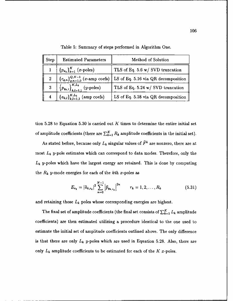
106
Table 5: Summary of steps performed in Algorithm One.
Step Estimated Parameters Method of SolutionK
1 {P}ik=l (x-poles) TLS of Eq. 5.6 w/ SVD truncation
2 lCq,n}Q,-1 (x-amp coefs) LS of Eq. 5.16 via QR decompositionSK,Lk
3 P t k, , 1 (y-poles) TLS of Eq. 5.24 w/ SVD truncation
4 {a,,i} 1,Lk (amp coefs) LS of Eq. 5.28 via QR decomposition
tion 5.28 to Equation 5.30 is carried out K times to determine the entire initial set
of amplitude coefficients (there are E]g= Rk amplitude coefficients in the initial set).
As stated before, because only Lk singular values of Pk are nonzero, there are at
most Lk y-pole estimates which can correspond to data modes. Therefore, only the
Lk y-poles which have the largest energy are retained. This is done by computing
the Rk y-mode energies for each of the kth x-poles as
N-1
Erk = Iak,1I rk = 1,2,..., Rk (5.31)n=-0
and retaining those Lk poles whose corresponding energies are highest.
The final set of amplitude coefficients (the final set consists of Lk amplitude
coefficients) are then estimated utilizing a procedure identical to the one used to
estimate the initial set of amplitude coefficients outlined above. The only difference
is that there are only Lk y-poles which are used in Equation 5.28. Also, there are
only Lk amplitude coefficients to be estimated for each of the K x-poles.

107
Algorithm Two
Algorithm Two uses the first three steps of Algorithm One twice, and then re-
quires a matching step and a final amplitude coefficient calculation step. The steps
involved in Algorithm Two are summarized in Table 6. The first three steps of Al-
gorithm One are carried out using the data d'(m, n) yielding x and y-pole estimates,
PK Lk{p,}~1 and teaasdt(n_k=l {PkII}=1- Next, the data is transposed (i.e. d" (n,m) = d'(m, n)), and
Algorithm One is applied to d't(n, m) to arrive at a second set of poles, {P, }k,=1
and { }~t" Note that the model orders K and Lk are related to Kt and Lt,
depending on the structure of a particular model, and are in general different. Also
note that included with steps 3 and 6 (which involve the estimation of the y and
yt-poles) of Algorithm Two is an amplitude coefficient estimation procedure in or-
der to determine the highest energy modes. This is required to insure that only the
correct number of true modes are retained in each step.
The two sets of estimates are combined, and the more accurate part of the
estimates from each set is retained. The more accurate part of each estirn ite is the
set of poles which were estimated first, (i.e. the x-poles from each set). The y-poles
are less accurate than the x-poles because they are estimates based on the x-pole
estimates. A matching algorithm is used to combine both sets of pole estimates
yielding a single set of pole estimates.
The matching is performed using the following metric
(Pk ))= I'IP;k - P(tk',l, ,2 + Y- P0,1 (5.32)
Sexponentialesti-for the distance between 2-Dexonta modes/(Pk IPYk,.I) and (P k,,' .' estti-)
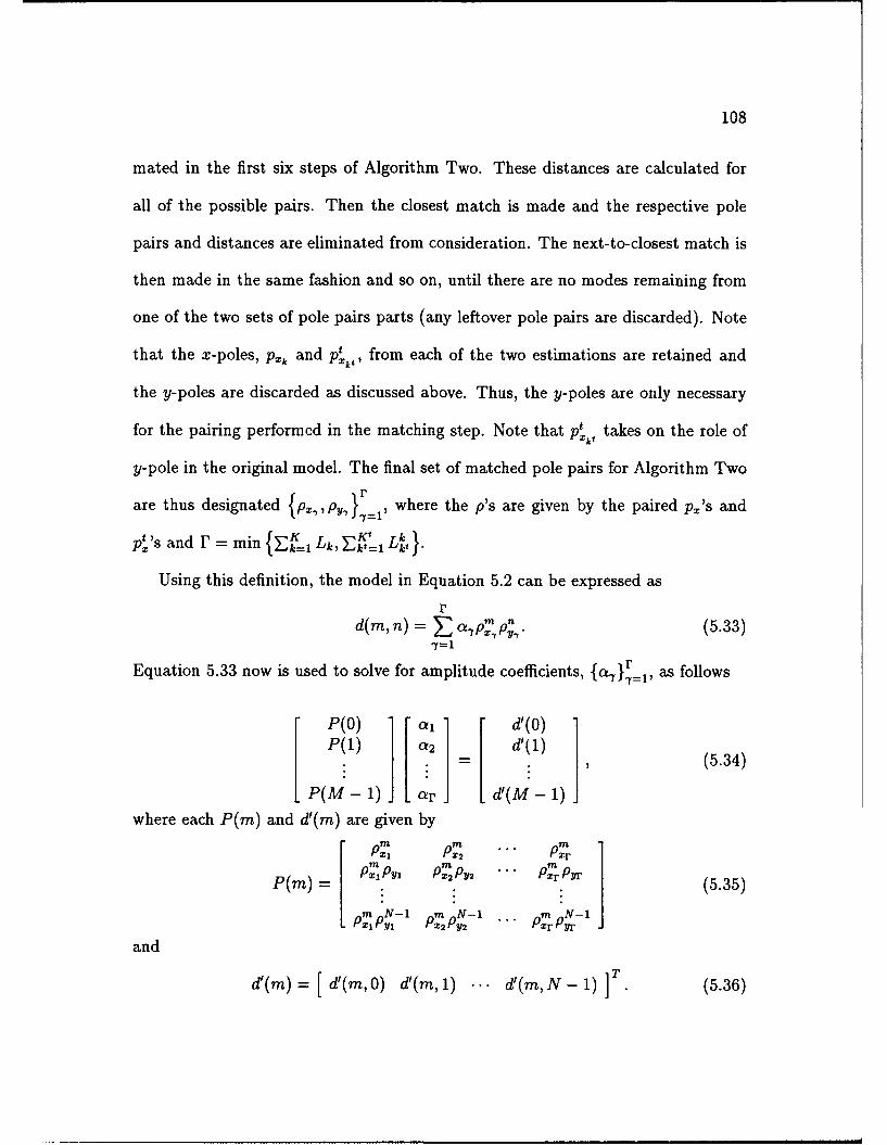
108
mated in the first six steps of Algorithm Two. These distances are calculated for
all of the possible pairs. Then the closest match is made and the respective pole
pairs and distances are eliminated from consideration. The next-to-closest match is
then made in the same fashion and so on, until there are no modes remaining from
one of the two sets of pole pairs parts (any leftover pole pairs are discarded). Note
that the x-poles, pk and p', from each of the two estimations are retained and
the y-poles are discarded as discussed above. Thus, the y-poles are only necessary
for the pairing performed in the matching step. Note that pt takes on the role of
y-pole in the original model. The final set of matched pole pairs for Algorithm Two
are thus designated {P,P, pY-T =, where the p's are given by the paired p,'s andpt's and F = min{ iLkt Lk.
Using this definition, the model in Equation 5.2 can be expressed as
rd(m, n) = >j aypp,,.m (5.33)
-y=l
Equation 5.33 now is used to solve for amplitude coefficients, {ay}r,, as follows
P(0) a [ d'(0)P(1) a2 = d'(1) (5.34)
P(M- 1) ar d'(M- 1)where each P(m) and d'(m) are given by[ ... 1PX1 P2 "' PrPr
P(M) P 2 ... :: : (5.35)
m N-l m pN- ... pm pN- 1P., Py, P-2 Py2 " "Pr PYr
and
d'(m) " [ d'(m,0) d'(m, 1) ... d'(m,N- 1) ]T. (5.36)
109
Table 6: Summary of steps performed in Algorithm Two.
fl Step Estimated Parameters Method of Solution
{Px=}1 (x-poles) TLS of Eq. 5.6 w/ SVD truncation
2 { cq,l,n-1 (x-amp coefs) LS of Eq. 5.16 via QR decomposition
3 {Pyk,, I gK' Lk (y-poles) TLS of Eq. 5.24 w/ SVD truncation
4 P t , t (xtpoles) TLS similar to Step 1
Ic ,Q{M, 1 , (xt-amp coefs) LS similar to Step 2
6't (yt-poles) TLS similar to Step 314,1 kt ,lt=I,I
7 2p 1 j31' r (x and y-poles) Matching using Eq. 5.32
8 {,,}r:1 (amp coefs) LS of Eq. 5.34 via QR decomposition
Equation 5.34 can be expressed as
PA = D'. (5.37)
The amplitude coefficients are found using the pole estimates from a least squares
solution to Equation 5.34 which can be written as
A = (f>H )' '. , (5.38)
although numerically more robust solutions (using, e.g., the QR decomposition [56])
are preferred to direct computation of Equation 5.38.
110
Implementation Issues
In this section operation counts for the four steps of Algorithm One and for the
eight steps of Algorithm Two are presented. These operation counts are given for
the case when the data is real. For complex data considered in the examples which
follow the counts were observed to be about a factor of 2 to 3 larger for the SVDs
and about 4 times larger for the QR decompositions. An alternative to the larger
SVD steps is presented which provides a reduction in computation.
Operation Count for Algorithm One. To obtain the operation counts for the
four steps of Algorithm One, the counts for the SVD computations and the compu-
tation of the QR decompositions used for the least squares solutions are needed.
The approximate floating point operation (flop) count, fcSVD, associated with
the computation of the singular values and left singular vectors of a real r x c matrix
is given by fcSVD - 4rc2 + 8c 3 [56]. Thus the flop count for the SVD of Step 1,
fCne, is given by
fcbne 4N(M - Q)(Q + 1)2 + 8 (Q + 1)'. (5.39)
The approximate flop count, fcQR, associated with the QR decomposition of a real
r x c matrix is given by fcQR ; 2rc2 - dc3 [56]. Thus, the flop count for the QR
decomposition required for the LS solution of Step 2 is given by
One M Q3.

111
For the K SVDs in Step 3 the approximate flop count is given byK
One E"(4(N-Rk) (Rk 8(Rk+ )). (5.41)k=1
For the K QR decompositions in Step 4 the approximate flop count is given by
fc4~ Z2NR 2 _ (5.42)
The flop count for the SVDs and QR decompositions of Algorithm One is given
by the sum of the individual flop counts above.
To achieve near optimal performance (with respect to the Cram~r-Rao Bound
(CRB)), the model order used for Steps 1 and 3 of Algorithm One should be integers
near Q = m and Rk = - [59]. Using these substitutions and further approximations
the estimate for the total flop count is
fCOne,- - 1 M3N + 1KN3. (5.43)fne 3 2 (.3
Note that the K estimations of Steps 3 and 4 are independent of each other and can
thus be done in parallel.
Operation Count for Algorithm Two. Since Algorithm Two first uses the firstthree steps Algorithm One fc' = fc , fC2 - fc2 and fc3 - fc3 for the
T o =fOnes T one, andT One
flop counts of those steps. For Steps 4-6, the roles of M and N are reversed, and
Qt and RL are used instead of Q and Rk. Their flop counts are thus
fC,4wo 4M(N - Q)(Qt + 1)2+8 (Qt+I)3
fC5 2NQ,202t3fCTwo 3 2NQt2 -
fCw K (4 (M - R.,) (R, + 1)2 + 8 (Rt, + 1) 3). (5.44)kt=l
112
Each distance (A(., .)) calculation requires 16 flops. Thus, the flop count for Step 7
is given byK K0
fCwo = 16 Lk j L k (5.45)k=1 k1=1
For the QR decomposition in Step 8 the approximate flop count is given by
fC8 ; 2MNr 2 - 2 0. (5.46)Two 3
The flop count for the SVDs, QR decompositions, and matching of kl-rithm Two
is given by the sum of the individual flop counts above.
Again, to achieve near optimal performance (with respect to the CRB), the
model order used for Steps 1, 3, 4, and 6 of Algorithm Two should be integers
near Q = R, = 3, Rk = = N [59]. Using these substitutions and further
approximations the total flop count is estimated as
fCTwo - 1 M 3N + 1 KN3 + 1 N3M + 1 KtM3 + 2MNF2 - 20. (5.47)3 2 3 2 3
Note that the number of flops required for Step 7 is negligible when compared to
the other steps. Also note that the K estimations of Step 3 are independent and
the Kt estimations of Step 6 are independent and can thus be done in parallel.
Alternative Method for x-pole Estimation. The solution for b using Equa-
tion 5.5 can become computationally intensive for large data sets. For example, if
M = N = 64 and Q = 20, then S is of dimension (2816 x 21). Since only the right
singular vectors and the singular values are needed, one can instead obtain b from
113
a related eigen-decomposition problem. Consider S'S,
H1SHS = 1 Si 1 S'S 2 (.8
[S2 S 1 S2 S2 j '
where s, is the first column of S and S 2 are the remaining Q columns (i.e. S =
[ S1 S2 ]). Note that for typical problems S contains many more rows than
columns, so SHS is smaller than S. An eigen-decomposition of SHs is performed,
and all but the K largest eigenvalues are truncated to give SHS. Finally the mini-
mum norm estimate of b is given by,
= H- (sHS2 ) + s 1 (5.49)
where $2SS2 and S2s1 are the lower right and lower left submatrices of SHS, re-
spectively (cf. see Equation 5.48).
Note that this procedure is less numerically accurate than the previous procedure
because of the squaring of the data (which occurs in SHS), so extended precision
should be used in the computations.
5.2.4 Examples
Below numerical examples are presented to assess model validity and noise effects.
Two examples are presented. The first example considers the estimation of three
2-D undamped exponentials; this example was also considered in [28]. The second
example considers the estimation of three 2-D damped exponentials.
114
Example 1
In this example the variances of frequency and magnitude estimates are compared
to their Cram~r-Rao Bounds (CRBs) at various signal to noise ratios (SNRs) for
the three 2-D frequency scenario presented in [28] using Algorithm One and Algo-
rithm Two. Data was generated using the model in Equation 5.2 for M = N = 20
and
p, a,,,]= e i2 7r0*24 e 32wx24 13
[PX1 P, 2 al,2 3=[ei21rO 24 ei2wO.26 13
[PX,2 p12,1 a2,1 e = e 27r0 26 ej2 7rO.24 1].(5.50)
It can see that from the angles of the above poles the corresponding frequencies are
0.24 and 0.26. For the purposes of identification the (x-pole,y-pole) pairs above are
labeled with frequencies (0.24,0.24), (0.24,0.26), and (0.26,0.24) as 2-D frequencies
fl, f2, and f3, respectively. Note that these frequencies are spaced at four-tenths
of a Fourier bin in both directions (1 Fourier bin= -I- = 0.05). Also note that this20
data consists of undamped exponentials. These 2-D frequencies are shown on the
2-D frequency plane in Figure 45.
Figures 46(a) and 46(b) show the simulation results for the x-pole frequencies
and y-pole frequencies, respectively where Algorithm One was used. One hundred
different noise realizations were run for each integer SNR between 0 and 50dB. The
SNR is defined as the total signal power divided by the total noise power. Specifically
these figures show the estimated frequency variances for the various SNRs (they are
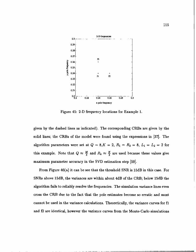
115
2-D freqeuncies0.3
0.29
0.28
0.27S
0 .26 +
0.25
0.24 +
fl f20.23
0.22
0.21
0.20.2 0.22 0.24 0.26 0.28 03
x-pole frequency
Figure 45: 2-D frequency locations for Example 1.
given by the dashed lines as indicated). The corresponding CRBs are given by the
solid lines; the CRBs of the model were found using the expressions in [37]. The
algorithm parameters were set at Q = 8,K = 2, R 1 = R2 = 8, L1 = L2 = 2 for
this example. Note that Q ;K and Rk N are used because these values give
maximum parameter accuracy in the SVD estimation step [59].
From Figure 46(a) it can be see that the threshold SNR is 15dB in this case. For
SNRs above 15dB, the variances are within about 4dB of the CRB; below 15dB the
algorithm fails to reliably resolve the frequencies. The simulation variance lines even
cross the CRB due to the fact that the pole estimates become so erratic and most
cannot be used in the variance calculations. Theoretically, the variance curves for fl
and f2 are identical, however the variance curves from the Monte-Carlo simulations
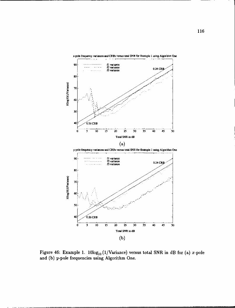
116
x-pole frequency variances and CRBs versus tota SNR for Example 1 using Algorithm One
90 - --------- fl variance
-------- frqunc variances an0.sv24sttlSN o xm le1ui Aloih n
- -- - - - - fB variance
80-
70-- . -
50
0 5 10 15 20 25 30 35 40 45 50
Total SNR in dBE
(b)
ad() y-pole frequencs ine n R~ essttlSN o xml using Algorithm One

117
separate at the lower SNRs due to differences in the y-pole estimates which cause
some outliers to not be included in the variance calculations. The results in [28]
are for an SNR per pole of 10dB, which corresponds to a total SNR of 17.7dB used
here. In comparison, the estimation scheme in [28] gives x-pole frequency variances
which are about 3 or 4dB better for fl and fM and about 8dB better for f2.
Figure 46(b) is a plot of the inverses of the y-pole frequency variances for the
various SNRs along with the corresponding CRBs as before. From this figure it
can be see that the curve for the y-pole variance for fM exhibits the same properties
as those discussed for the x-pole frequency variances above. The y-pole frequency
variances for fl and f2 are about 13 and 10 dB away from their respective CRB
lines, respectively. Also, the y-pole estimation for fl and f2 breaks down at SNRs
below 25dB. The fact that these variances are farther away from their CRBs and
that the resolution threshold is higher is expected because of the accumulation of
error which occurs in the y-pole estimates in Algorithm One. This accumulation of
error does not occur in Algorithm Two, as shown below.
Figure 47 shows the estimated x-pole and y-pole magnitude variances for this
example when Algorithm One is used. The characteristics are the same as those for
the frequency variances, with respect to the CRBs.
Figure 48 shows the estimated x-pole and y-pole frequency variances for this
example when Algorithm Two is used. As expected, the x-pole frequency variances
are much the same as those for Figure 46(a), but the y-pole frequency variances
have been improved to match the x-pole frequency variance performance. The esti-
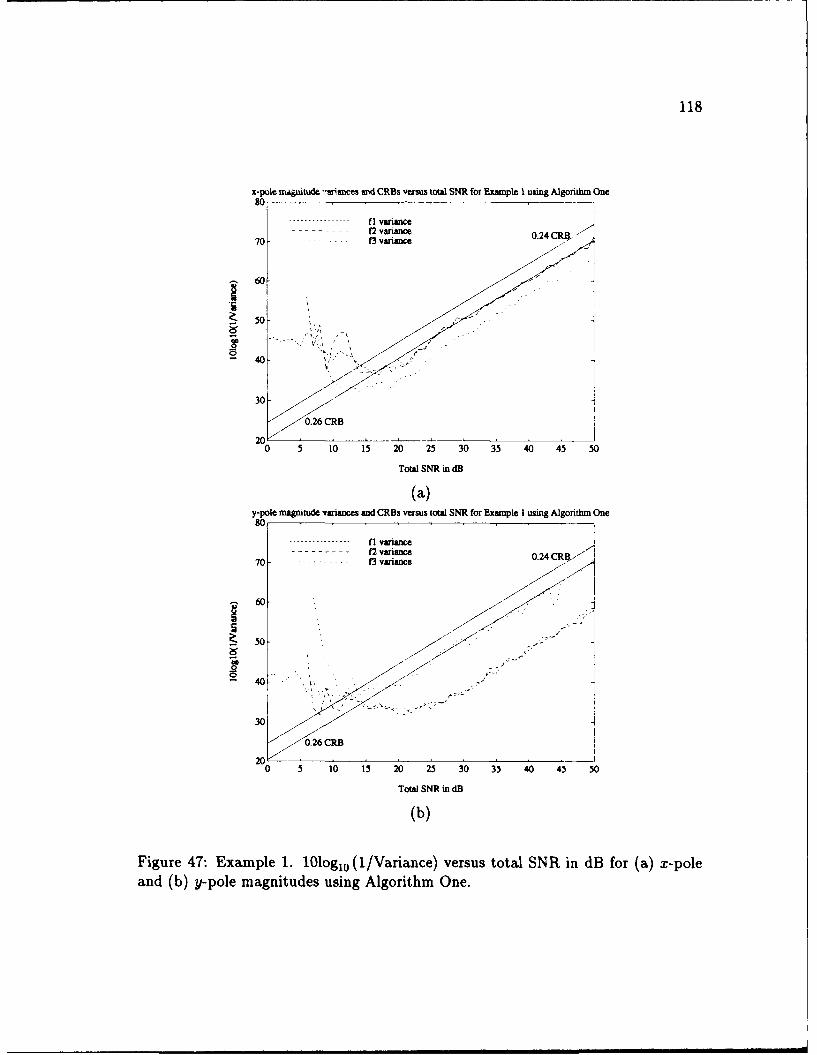
118
x-pole magiude -ariances and CRBS versus total SNR for Example I using Algorithm One8C
--------- fl variance------ Qvariance 0.24 CR~l -
650
501
30
0.26 CIR8
200 5 10 15 20 25 30 35 40 45 50
Total SNR in dB
(a)y-pole magnitude variances and CRBs versus total SNR for Example I using Algorithm One80
----- ----- ---- fI variance---------- 2 variance 02 R , ,
70- f3 vari0.4nce
~60-
500
40.f-
30-
20 0.26 CR8 .
0 5 10 15 20 25 30 35 40 43 50
Total SNR in dB
(b)
Figure 47: Example 1. 10logl 0 (1/Variance) versus total SNR in dB for (a) x-poleand (b) y-pole magnitudes using Algorithm One.
119
mation scheme in [28] gives variances which are about 3 or 4dB better for the y-pole
frequencies of fl and f2 and variances which are about 8dB better for the y-pole
frequency of f3.
Figure 49 shows the estimated x-pole and y-pole magnitude variances for this ex-
ample when Algorithm Two is used. The improvements in the magnitude estimates
are comparable to the improvements in the frequency estimates.
Next consider the SVD operation counts for this example for Algorithm Two.
The SVD steps are major computational parts. Each noise realization required SVDs
of two 240 x 9 matrices and four 9 x 11 matrices where only the singular values and
right singular vectors were computed. For the same example, the algorithm in [28]
required SVDs of two 49 x 169 matrices for each noise realization where the singular
values and left singular vectors are computed. Looking at expressions in [56] for
SVD computations, Algorithm Two requires fewer flops than the algorithm in [28]
for the SVDs. Note that the SVDs for both algorithms can be performed with fewer
computations by computing the eigen-decomposition of smaller square matrices as
discussed in Section 5.2.3. Using this idea the total number of computations are
reduced for both methods, however there is still savings with Algorithm Two over
the algorithm in [28].
Example 2
In this example the estimation of damped exponentials in noise is examined us-
ing Algorithm Two. Data was generated using the model in Equation 5.2 for
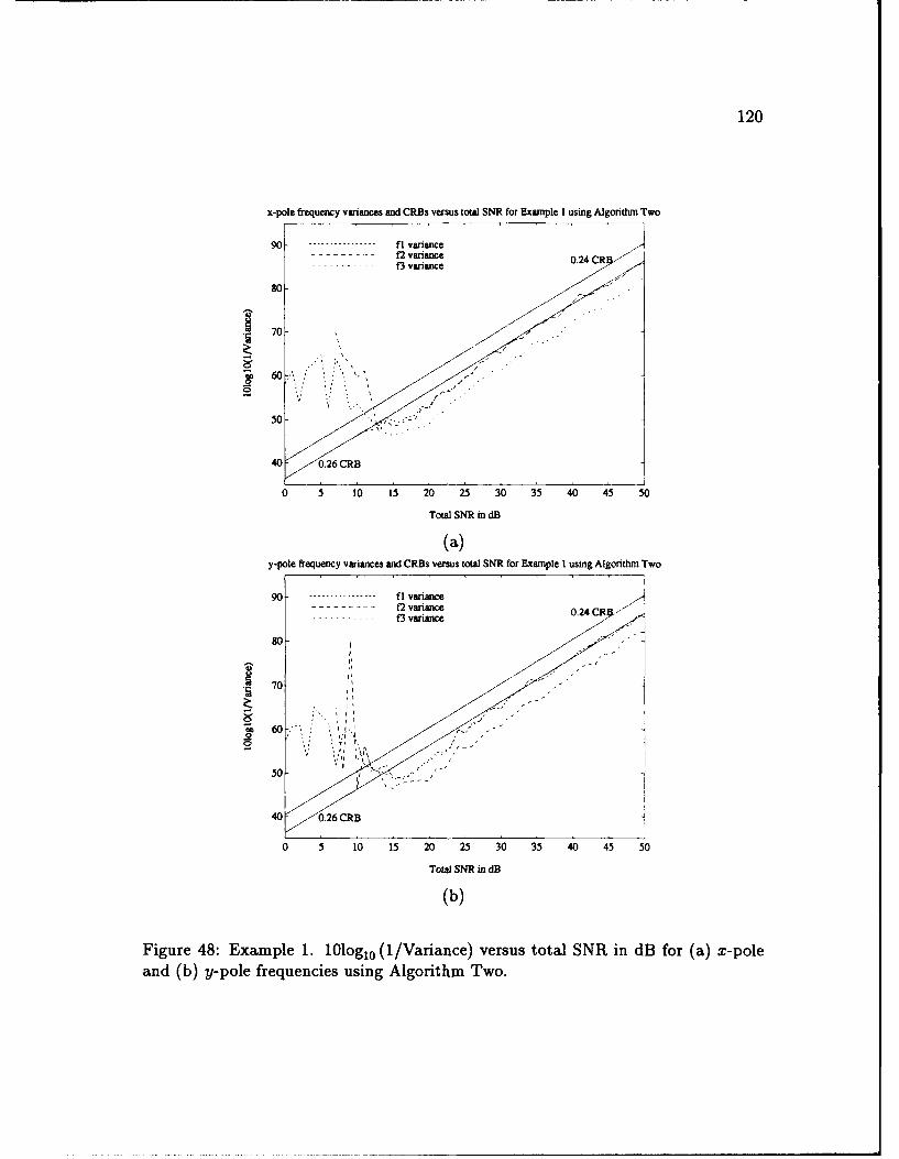
120
x-pole frequency variances and CR~s versus total SNR for Example I using Algorithm Two
90 - --- ------ f variance----- f2 variance 0.24 C
50
0 5 10 15 20 25 30 35 40 45 50
Total SNR in dB
(a)y-pole frequency variances and CRBs versus total SNR for Example I using Algorithm Two
90 -------- Hi variance----- f2 variance 0.24 CR X------ ---- 3 variance
0
0 5 10 15 20 25 30 35 40 45 50
Total SNR in dB
(b)
Figure 48: Example 1. l0logl0 (1/Variance) versus total SNR in dB for (a) x-poleand (b) y-pole frequencies using Algorithm Two.
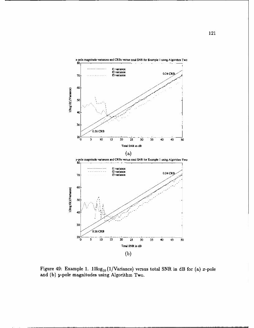
121
x-pole magnitude variances and CR~s versus total SNR for Example I using Algorithm Twoso
---- - --- fl variance---- f2 variance
70- ------ Svrac 0.24 C
60 -
40
0 5 10 15 20 25 30 35 40 45 50
Total SNR in dB
(a)y-pole, magnitude variances and CRBs versus total SNR for Example I using Algorithm Two
60-
00.24 CRB
20
0 5 10 15 20 25 30 35 40 45 50
Total SNR in dB
(b)
Figure 49: Example 1. 101ogl 0 (1/Variance) versus total SNR in dB for (a) x-poleand (b) y-pole magnitudes using Algorithm Two.
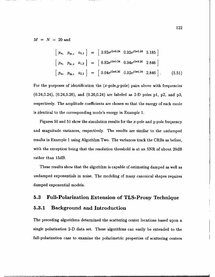
122
M = N =20 and
[px, py, 1 a,,,]= 0.92e j2 , 0-24 0.92e j2x0 .24 3.185]
[X P 112 al,2 ] 0 .92e32,x0.24 0.94e j2 1r. 26 2.846
PX2 py, a2,1 ]=[0.94e2 ,rO.26 0.92e j2 wO.24 2.846 ]. (5.51)
For the purposes of identification the (x-pole,y-pole) pairs above with frequencies
(0.24,0.24), (0.24,0.26), and (0.26,0.24) are labeled as 2-D poles pl, p2, and p3,
respectively. The amplitude coefficients are chosen so that the energy of each mode
is identical to the corresponding mode's energy in Example 1.
Figures 50 and 51 show the simulation results for the x-pole and y-pole frequency
and magnitude variances, respectively. The results are similar to the undamped
results in Example 1 using Algorithm Two. The variances track the CRBs as before,
with the exception being that the resolution threshold is at an SNR of about 20dB
rather than 15dB.
These results show that the algorithm is capable of estimating damped as well as
undamped exponentials in noise. The modeling of many canonical shapes requires
damped exponential models.
5.3 Full-Polarization Extension of TLS-Prony Technique
5.3.1 Background and Introduction
The preceding algorithms determined the scattering center locations based upon a
single polarization 2-D data set. These algorithms can easily be extended to the
full-polarization case to examine the polarimetric properties of scattering centers
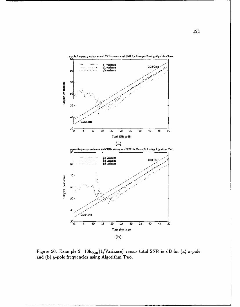
123
x-pole frequency variances and CRBs versus total SNR for Example 2 using Algorithm Two90
- --------- p1 variance- -- - - p2 variance 0.24 C
go - -- ---- p3 variance
70-
0 5 10 15 20 25 30 35 40 45 50
Total SNR in dB
(a)y-pole frequency variances and CRBs versus total SNR for Example 2 using Algorithm Two90
------- Tot-- S R iniac dZ
Figure------ 50: Eape210g 0 (/variance) versu toalSR i Bfr()x landg (b --------- frqunce usng agrithmTwo
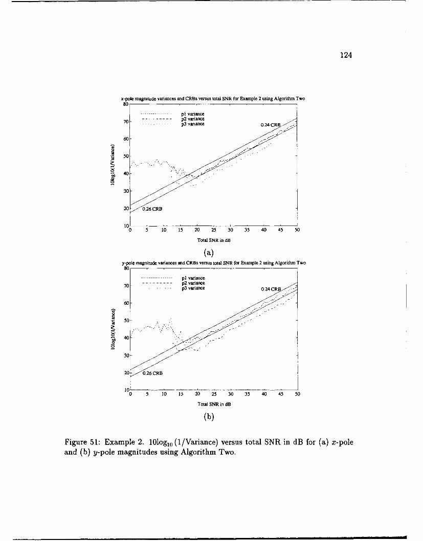
124
x-pole magnitude variances and CRBs versus total SNR for Example 2 using Algorithm Two80
--- I --- --- -- p1 variance70- -- ------ p2variance
70 --- p3 variance 0.24 CRB
0 6010
20- 0.26 CRB
10 5 10 15 20 25 30 35 40 45 50
Total SNR in dB
(a)y-pole magnitude variances and CRBs versus total SNR for Example 2 using Algorithm Two
80
60
20- 0.26 CRIB
0 5 10 15 20 25 30 35 40 45 50
Total SNR in dB
(b)
Figure 51: Example 2. 101ogl0 (1/Variance) versus total SNR in dB for (a) x-poleand (b) y-pole magnitudes using Algorithm Two.
125
on a 2-D image. A method to examine full-polarization data is presented which is
based on the concept of a transient polarization response (TPR) [4, 35, 36]. Ac-
cording to the TPR concept, the target is illuminated with an impulsive circularly
polarized electromagnetic wave, and as the wave interacts with each scattering cen-
ter on the target, each scattering center will reflect back a wave with a polarization
which is determined by the polarimetric characteristics of that scattering center.
This concept has been investigated in 1-D for both nonparametric [4, 35, 36] and
parametric [37, 38] techniques. The nonparametric techniques use the IFFT of the
full-polarization stepped frequency data to form the TPR of a target. The peaks in
the TPR profile give the scattering center locations. Polarization ellipses are then
given by the polarization properties of the TPR at the scattering center locations.
Thus, the amplitude and orientation of each ellipse characterize the polarimetric
properties of each scattering center. Parametric techniques employing the 1-D TLS-
Prony technique described in Chapter IV have been developed for the TPR [37, 38].
This technique has the advantage of higher resolution than the IFFT method and
of direct estimation of the scattering center locations.
The technique presented here is a 2-D extension of the 1-D TLS-Prony based
parametric TPR technique developed in [37, 38]. The 2-D TLS-Prony Technique
algorithms previously presented, with slight modifications, are used to determine
the scattering center locations and amplitude coefficients. The ellipse parameters
are then calculated from the amplitude coefficients.
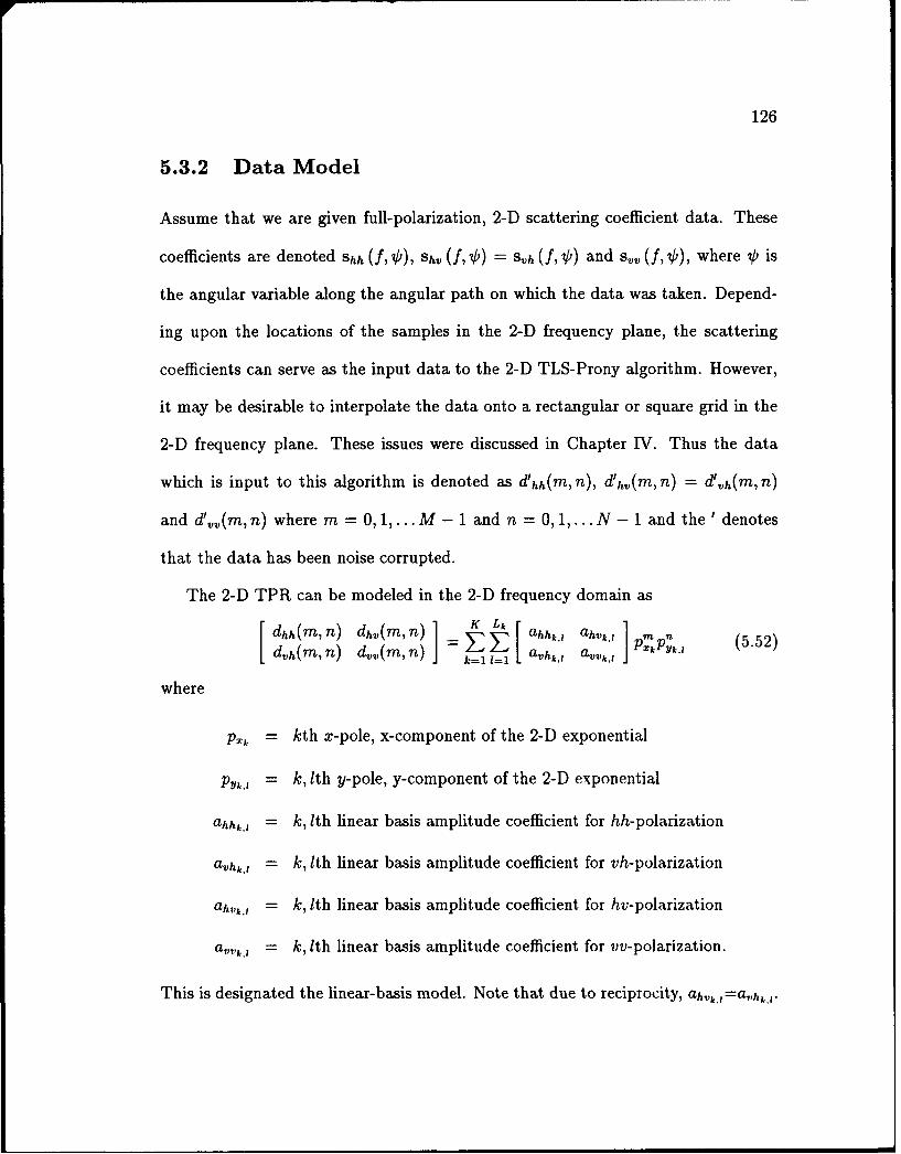
126
5.3.2 Data Model
Assume that we are given full-polarization, 2-D scattering coefficient data. These
coefficients are denoted Shh (f,4'), Sh (fU, ) = S h(f, 4) and s, (f, 4), where 0 is
the angular variable along the angular path on which the data was taken. Depend-
ing upon the locations of the samples in the 2-D frequency plane, the scattering
coefficients can serve as the input data to the 2-D TLS-Prony algorithm. However,
it may be desirable to interpolate the data onto a rectangular or square grid in the
2-D frequency plane. These issues were discussed in Chapter IV. Thus the data
which is input to this algorithm is denoted as d'hh(m, n), d'h,(m, n) = d'vh(m, n)
and d',(m, n) where m = 0, 1,... M - 1 and n = 0, 1,... N- 1 and the ' denotes
that the data has been noise corrupted.
The 2-D TPR can be modeled in the 2-D frequency domain as[dhh(m, n) dh,(m, n) 1 KL ahhk,l ahVk, 1' nm5.2dvh(m, n) d.~(m, n) l l. l avhk avvk,t X J .
where
P~k = kth x-pole, x-component of the 2-D exponential
P~kI = k, th y-pole, y-component of the 2-D exponential
ahhk, = k, lth linear basis amplitude coefficient for hh-polarization
avh , = k, th linear basis amplitude coefficient for vh-polarization
ahVk, t = k, ith linear basis amplitude coefficient for hv-polarization
a,,vk' = k, Ith linear basis amplitude coefficient for vv-polarization.
This is designated the linear-basis model. Note that due to reciprocity, ah,,k.a=a,,hkj,.
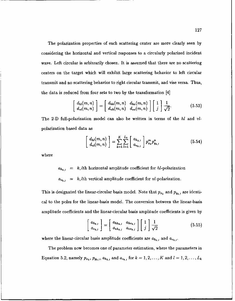
127
The polarization properties of each scattering center are more clearly seen by
considering the horizontal and vertical responses to a circularly polarized incident
wave. Left circular is arbitrarily chosen. It is assumed that there are no scattering
centers on the target which will exhibit large scattering behavior to left circular
transmit and no scattering behavior to right circular transmit, and vise versa. Thus,
the data is reduced from four sets to two by the transformation [4]
dhl(m, dhh(m,) dh,(m,n) (5.53)d,d(m, n) [ dh(m,n) dhj(m,n)Jd m j -5.3
The 2-D full-polarization model can also be written in terms of the hl and vi-
polarization based data as
rdhl (m, n) [ L ahkl, 1 m=EEmn aV,1 " (5.54)1k=l !=1avt
where
ah,, = k, Ith horizontal amplitude coefficient for hi-polarization
av., = k, Ith vertical amplitude coefficient for vl-polarization.
This is designated the linear-circular basis model. Note that pk and PYk., are identi-
cal to the poles for the linear-basis model. The conversion between the linear-basis
amplitude coefficients and the linear-circular basis amplitude coefficients is given by
[ahk 1 ahhk, ah,,k, (555ak = avhk, a,,,k, J55
where the linear-circular basis amplitude coefficients are ahk,, and a,,k. *.
The problem now becomes one of parameter estimation, where the parameters in
Equation 5.2, namely Pk, Py,.,, ah,, and a,,,,, for k = 1, 2, ... , K and I = 1, 2,..., Lk
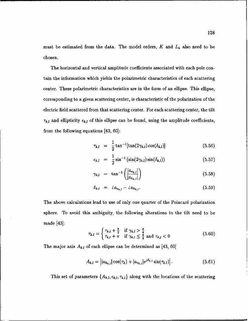
128
must be estimated from the data. The model orders, K and Lk also need to be
chosen.
The horizontal and vertical amplitude coefficients associated with each pole con-
tain the information which yields the polarimetric characteristics of each scattering
center. These polarimetric characteristics are in the form of an ellipse. This ellipse,
corresponding to a given scattering center, is characteristic of the polarization of the
electric field scattered from that scattering center. For each scattering center, the tilt
rk,l and ellipticity Ek, of this ellipse can be found, using the amplitude coefficients,
from the following equations [43, 60]:1
Tk,l = 1 tan-[tan(2k,l)cos(bk,)] (5.56)2
_k,1 1 sin 1 (sin(27k,) sin(bk,l)) (5.57)E t 2
'Yk,l = tan-1 (IavklI' (5.58)
6k,I = /a,,l - Zahk.,. (5.59)
The above calculations lead to use of only one quarter of the Poincar6 polarization
sphere. To avoid this ambiguity, the following alterations to the tilt need to be
made [43]:= rk,I + 2 if Yk,t-, (5.60)
Tk,t + ?r if 1ki < and <0(.
The major axis Ak,, of each ellipse can be determined as [43, 60]
Ak, = IahkI cos(rk) + la,,, lei'kl sin(rk,I) . (5.61)
This set of parameters {AkJ, Ek,j, k,i} along with the locations of the scattering
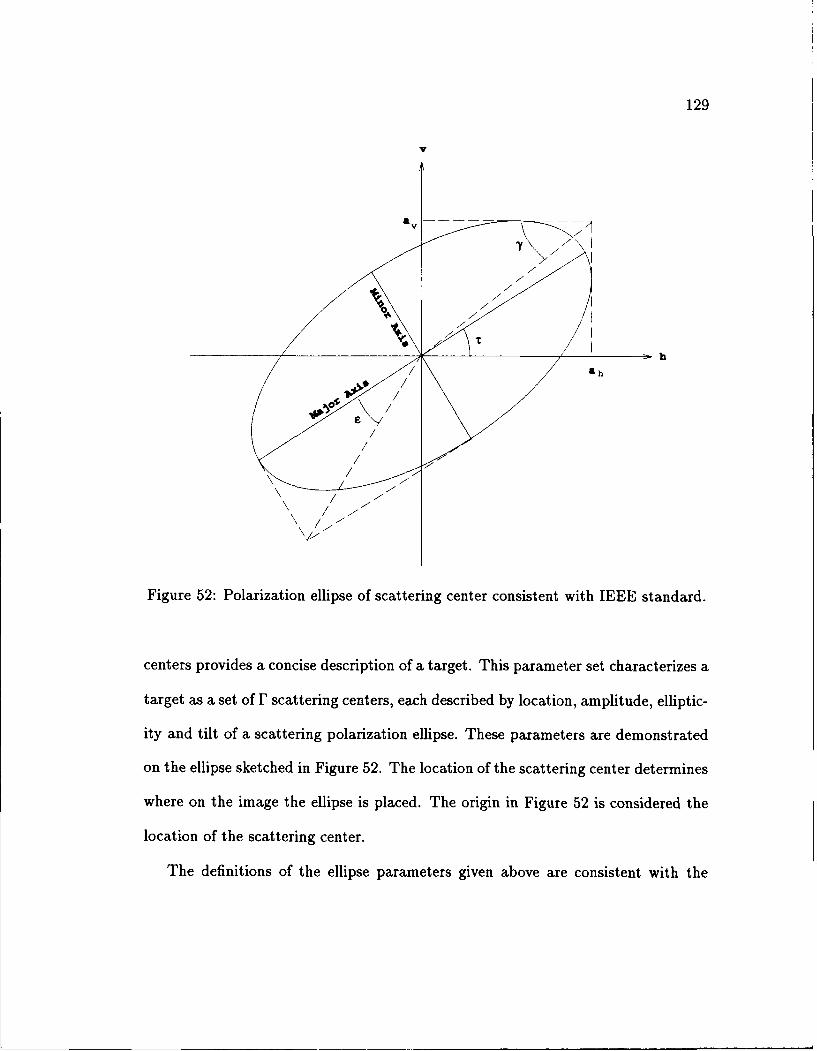
129
a
/ a h D
\ / - /--
Figure 52: Polarization ellipse of scattering center consistent with IEEE standard.
centers provides a concise description of a target. This parameter set characterizes a
target as a set of F scattering centers, each described by location, amplitude, elliptic-
ity and tilt of a scattering polarization ellipse. These parameters are demonstrated
on the ellipse sketched in Figure 52. The location of the scattering center determines
where on the image the ellipse is placed. The origin in Figure 52 is considered the
location of the scattering center.
The definitions of the ellipse parameters given above are consistent with the
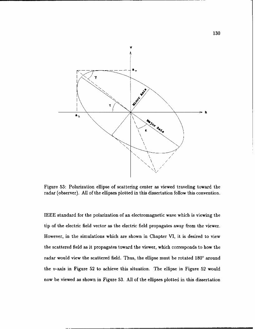
130
V
a h
K \ /
\\/
Figure 53: Polarization ellipse of scattering center as viewed traveling toward theradar (observer). All of the ellipses plotted in this dissertation follow this convention.
IEEE standard for the polarization of an electromagnetic wave which is viewing the
tip of the electric field vector as the electric field propagates away from the viewer.
However, in the simulations which are shown in Chapter VI, it is desired to view
the scattered field as it propagates toward the viewer, which corresponds to how the
radar would view the scattered field. Thus, the ellipse must be rotated 1800 around
the v-axis in Figure 52 to achieve this situation. The ellipse in Figure 52 would
now be viewed as shown in Figure 53. All of the ellipses plotted in this dissertation
131
follow the convention of Figure 53, assuming that the viewer is at the radar and the
scattered field is propagating toward the radar.
5.3.3 Estimation Algorithms
This section describes two algorithms for estimation of the x and y-poles along
with both sets of amplitude coefficients. The two full-polarization algorithms are
called Full-Polarization Algorithm One (FPA1) and Full-Polarization Algorithm
Two (FPA2). These algorithms are very similar to the single-polarization versions,
Algorithm One and Algorithm Two, which were presented earlier in this chapter.
The main differences are that there are two input data sets and that there are
two sets of amplitude coefficients to estimate in the full-polarization case. Also, an
additional step unique to the full-polarization case is the calculation of the ellipse
parameters from the parameter estimates. The two input data matrices are defined
as follows
dh(0, 0) dt(1, 0) ... d(M- 1, 0)
dhI(0, 1) dh, (1, 1) ... dh(M- 1,1) (5.62)h, (0, N - 1) dhi(1, Ni- 1) ... 1
and
d, 1(0, 0) d'1(1, 0) ... d,(M - 1,0)
D' = (5.63)
d',,((ON - 1) d',l1, N- 1) .. d,,,(i- 1, N- 1)
Moving across a row in D', or D', is considered moving in frequency while moving
down a column of either matrix is considered moving in angle in the 2-D frequency
plane.
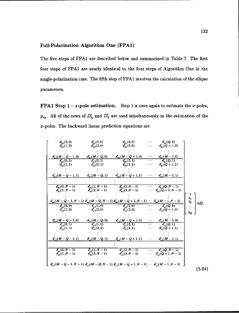
132
Full-Polarization Algorithm One (FPA1)
The five steps of FPA1 are described below and summarized in Table 7. The first
four steps of FPA1 are nearly identical to the four steps of Algorithm One in the
single-polarization case. The fifth step of FPA1 involves the calculation of the ellipse
parameters.
FPA1 Step 1 : x-pole estimation. Step 1 is once again to estimate the x-poles,
pX2 . All of the rows of D' and D' are used simultaneously in the estimation of the
x-poles. The backward linear prediction equations are
d'hl(0,0) dh (1, 0) d' ,(2, 0) -..- d'hI(Q,0)d I(1,0) dh,(2, 0) dh 1(3, 0) .. d'hI(Q + 1,0)
d' (M-Q - 1,0) dAI(M -Q,O) d ,(M - Q + 1,0) ... d 1,0(M-1,O)d 1,(0, 1) d1(1, 1) d -1(2, 1) ... d , (Q, 1)d -(1, 1) d (2, 1) d'h,(3, 1) ... d ,,(Q + 1, 1)
d'h,(M -. Q - 1, 1) d ,(M - Q, 1) d~,(M -. Q + 1,1) ... d'(M - 1, 1)
d,,(O,N - 1) d(1, N - 1) d (2, N - 1) ... d,,(Q,N - 1)d',(1, N -1) d(2, N - 1) dh(3, N - 1) ... d,,,(Q + 1,N-)
d',- Q - 1) d,,(M -Q, N- ) d,(M - d, + 1,0) - 1) b
d,(MI-Q -1,1)d(M-Q,N)d,(M-Q+ 1,N-1) -(M b2d't(0,0 ) d', (1, 0 ) d ,,(2, 0) ... d , (Q,O0).d' 1t(1, 0) dVI(2,0) d' ,,(3, 0) ... d'v;(Q + 1,0) b
d,(M - Q - 1,0) d',,t(M -Q,O) d:,,l(M -Q + 1,O) ... d:"(M -1,O)d'1 (0, 1) d. ,(1, 1) d'.,(2, 1) ... d',t(Q, 1)d , (1, 1) d , (2, 1) d' ,,(3. 1) ... d",,(Q + 1, 1)
d',(M - Q- 1, 1) d',(M -Q, 1) d,(M Q + 1I,1) ... d'l(M - 1 1)
d' (ON - 1) d N d',t(2, N - 1) d',(Q, N - 1)d,,IM N - 1) d',1(2, N - 1) d',(3, N - 1) d',,(Q + I,N - 1)
d'.,(M -Q- 1, N-1) d,,(M-Q, N-1) d,(M-Q+1,N-(1)...6 d,,,(M-1,N-1)(5.64)
133
or
Sh JL (5.65)
or
s [ o. (5.66)
The solution of the backward linear prediction equations and the x-pole estimates
are determined in a manner analogous to the manner outlined in Algorithm One,
Step 1 in Equations 5.6 to 5.13. The result is Q x-poles estimates.
As in Algorithm One, because only K singular values of S (the SVD truncated
version of S) are nonzero, there are at most K x-pole estimates which can correspond
to data modes. Therefore, only the K x-poles which have the largest energy will be
retained (as discussed in Step 2 below).
FPA1 Step 2 : x-amplitude estimation. The x-amplitude coefficients for the
full-polarization case are defined as
Chq," I 1= ahk7 ,(m,n) ]j P ' q = 1, 2,..., Q. (5.67)
With this definition, the model associated with Equation 5.54 using the estimated
x-poles is written as
d, (m, n) r 1,
I q=1 l~
where Chqn is the qth x-amplitude coefficient associated with the nth row of Dh and
where c q, is the qth x-amplitude coefficient associated with the nth row of D,.
Equation 5.68 is used to solve for the Ch,.ns and cf,.s using
134
P Z I P X 2
" " " P X Q C 1 0 C 17 ,1 C 17 1 ,N - - !
S2 ... 2 C2, C,1 °
C ]2,N- , T(5.69):Z •Z .. = D (569
PM- pM-1 ... PMQ- C'Q,0 C Q,1" C17QN-a
or
P.C, = D T. (5.70)
where
E {h, v}. (5.71)
Both sets of x-amplitude coefficients are found from least squares solutions to Equa-
tion 5.70 using the x-pole estimates.
As before, we retain only the K x-pole estimates with the highest energy, where
now the energy is defined as
N-I M-1
Eq = E I i q= 1,2,...,Q. (5.72)
The final x-amplitude coefficient estimates are found using a procedure identical
to the one used to determine the initial of x-amplitude coefficient estimates outlined
above. The only difference is that there are only K x-poles which are used in
Equation 5.69. Also, there are only Lk x-amplitude coefficients (per polarization)
to be estimated for each of the K x-poles.
FPA1 Step 3: Estimation of the y-poles. As in Algorithm One, the x-
amplitude coefficient estimates are now used to solve for the y-pole estimates. For
135
each of the K high energy x-poles, the backward linear prediction equations for the
model given by Equation 5.67 become
Chko Ch,l ... Chk,R,
Chk,l Chk, 2 ... Chk,Rk+l 1
b k
ChNR- ChkN-R h "'" eN_ b 2 0 k = 1,2,... ,K (5.73)Cvko Cvk, I ... CVk.Rk
Cvk,1 CVk, 2 ... CvkRk+1 b kL RkJ
CVk,N-Rk1l CVk,NRk Ck,N_1
or
FRk b] 0. (5.74)
The solution of the backward linear prediction equations and the y-pole estimates
are determined in a manner analogous to the manner outlined in Algorithm One,
Step 3 in Equations 5.25 to 5.27. The result is Rk y-poles estimates for each of the
K x-pole estimates.
As in the basic algorithm, because only Lk singular values of FRk (the SVD
truncated version of FR k ) are nonzero, there are at most Lk y-pole estimates which
can correspond to data modes. Therefore, only the Lk y-poles which have the largest
energy are retained (as discussed in Step 4 below).
FPA1 Step 4: Estimation of the Amplitude Coefficients. Now that all of
the required y-poles have been estimated, both sets of amplitude coefficients are
estimated next. Using Equation 5.67,
136
1 1 "". 1-c1,
P1k,I Ph,2 [.. P , a,1 Cmlk2 2 ... 2 a, , .2"'",l Py 2 P IR, C., 2 (5.75)
'N-1 N-1 N -I a- 7,,RCPyk, I PYA;,2 ... PYk.Rh CIU.JN-I
or
PkA = k (5.76)
where
7E {h, v}. (5.77)
Both sets of amplitude coefficients are found from least squares solutions to Equa-
tion 5.76 using the y-pole estimates along with the x-amplitude coefficient estimates.
As before, we retain only the Lk y-pole estimates with the highest energy for
each of the K x-poles, where now the energy is defined as
N-1
= 12kE 12n r, = 1, 2,..., Rk. (5.78)
The final amplitude coefficient estimates are found utilizing a procedure identical
to the one used to determine the initial of amplitude coefficient estimates outlined
above. The only difference is that there are only Lk y-poles which are used in
Equation 5.75. Also, there are only Lk amplitude coefficients (per polarization) to
be estimated for each of the K x-poles.
FPA1 Step 5: Calculation of the Ellipse Parameters. Now that all of the
poles and amplitude coefficients have been estimated, the ellipse parameters can be
determined from these estimates using Equations 5.56 to 5.61.

137
Table 7: Summary of steps performed in FPA1.
Sts Estimated Parameters Method of Solution
{P }k= (x-poles) TLS of Eq. 5.66 w/ SVD trunc.C QO,N-1
2 Chqn c, q,,"=Q10, (x-amp coefs) LS of Eqs. 5.69 via QR decomp.
3 {p'Ik,,l,7 1 (y-poles) TLS of Eq. 5.73 w/ SVD trunc.
aha K,Lk (amp coefs) LS of Eqs. 5.75 via QR decomp.
5 ,{ , (ellipse params) Eqs. 5.56 to 5.61171T,1, Ek)l, Ak,lltk,[=l , (lis aa
Full Polarization Algorithm Two (FPA2)
FPA2 extends FPA1 just as Algorithm Two extends Algorithm One in the single-
polarization case. FPA2 uses the first three steps of FPA1 twice, and then requires
a matching step and a final amplitude coefficient calculation step followed by the
ellipse parameter calculation step. The steps involved in FPA2 are summarized in
Table 8. The first three steps of FPA1 are carried out using the data d'hl(m, n) and
d',,I(m, n) yielding x and y-pole estimates, {Pk }k=1 and {P., }t. • Next, the data
is transposed (i.e. d'hlt(n,m) = d'hl(m,n) and d',vt(n,m) = d',I(m,n)), and FPA1
is applied to dhlt (n, m) and d" (m, n) to arrive at a second set of poles, {p, k,=1
and .}" Note that the model orders K and Lk are related to Kt and L'
depending on the structure of a particular model, and are in general different.
Just as in the single-polarization case, the two sets of estimates are combined,
and the more accurate part of the estimates from each set is retained. The match-
138
ing is performed in an identical manner to the single-polarization case using the
metric in Equation 5.32. The final set of matched pole pairs for FPA2 are thus
designated {p,,py }=, where the p's are given by the paired p 's and pts and
F= min { , 1 Lk, EK=l Lk
Using this definition, the model in Equation 5.54 can be expressed as
[ dhdrn n) ] = [~ ' ] 1fl (5.79)
Equation 5.79 now is used to solve for amplitude coefficients, {ah.,,, YY= as
follows
P(0) 1 d',1 (0)P(1) a .2 d',(1) (5.80)
P(M - 1) JLantr d'7(M - 1)
where each P(m) and d',(m) are given by
[ M~p ... P;MPrZ Pyl PM P ... " PM PyrP(m) = N-: ] (5.81)
M ^N-1 7a ^N-1 m ^N -1P2: Pyl PX PY2 Pxr Pyr
and
d',(m) = F d',(m,0) d',(m, 1) ... d'n(m,N- 1) ]T (5.82)
Equation 5.80 can be expressed as
PA = V,1'. (5.83)
where
qE {hl, vl} . (5.84)
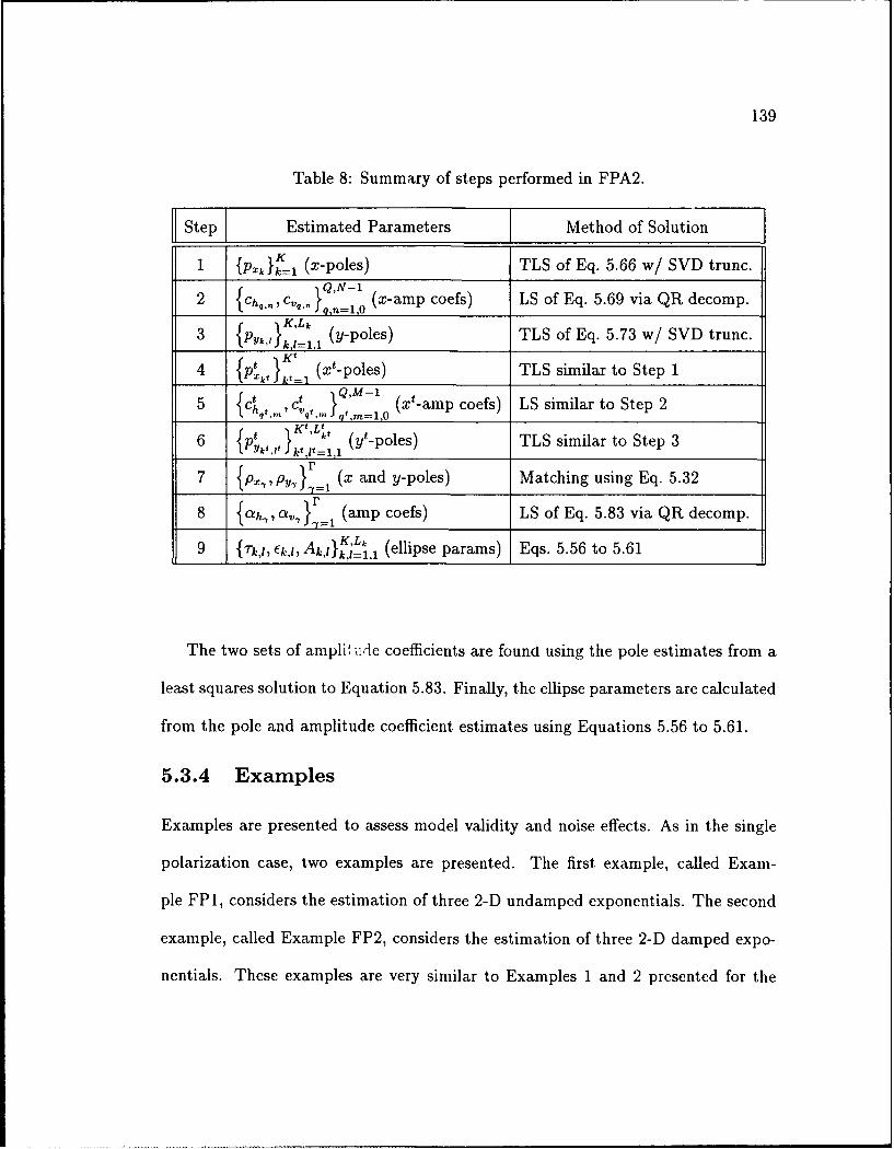
139
Table 8: Summary of steps performed in FPA2.
Step Estimated Parameters Method of Solution
{Pxk},l (x-poles) TLS of Eq. 5.66 w/ SVD trunc.
2 {Chgn ICq _Q,N-1 (x-amp coefs) LS of Eq. 5.69 via QR decomp.n =K,L&
3 PYkK k, (y-poles) TLS of Eq. 5.73 w/ SVD trunc.
4_ t Kt (xt-poles) TLS similar to Step 1I P l'XV Ikt
= 1
Ct t Q, (Mt-amp coefs) LS similar to Step 2
6gL'kt (yt-poles) TLS similar to Step 36 pykltt Jkt~lt=l 1
{p2 , p}r (x and y-poles) Matching using Eq. 5.32
8 {ah,, av, }IT (amp coefs) LS of Eq. 5.83 via QR decomp.
9 {TkEi, AWK'}If 1 (ellipse params) Eqs. 5.56 to 5.61
The two sets of ampli, ude coefficients are found using the pole estimates from a
least squares solution to Equation 5.83. Finally, the ellipse parameters are calculated
from the pole and amplitude coefficient estimates using Equations 5.56 to 5.61.
5.3.4 Examples
Examples are presented to assess model validity and noise effects. As in the single
polarization case, two examples are presented. The first example, called Exam-
ple FP1, considers the estimation of three 2-D undamped exponentials. The second
example, called Example FP2, considers the estimation of three 2-D damped expo-
nentials. These examples are very similar to Examples 1 and 2 presented for the
140
single polarization case.
Example FP1
In this example the variances of frequency and magnitude estimates are compared
to their CRBs at various signal to noise ratios (SNRs) for a three 2-D frequency
scenario (similar to the one presented in Example 1 earlier in this chapter) utilizing
FPA2. Data was generated using the model in Equation 5.54 for M = N = 20 and
[px1 py, ah,,, a,,,, e = e 2"0*24 e j21rO 24 1 i_]
[X PYp,,2 ah,2 a,, e j2'rO24 e j2TO.26 j12~~ 2 1 2 2
P 2 P, 2,1 ah2,1 a,2,1 I = [ 7~'0 6 " 2 F /2j-]. 5.5
The linear basis amplitude coefficients corresponding to the linear-circular basis
amplitude coefficients above are
ahhl,, ahv,, av,,, 1 0 1
ahhl.2 ahv,,2 a,,,,1,2 1 0 1
ahh2.1 al,,,, av,,, 1 1 0 1 ].(5.86)Recall that ah,,k,=a,,hk,1.
It can be seen that from the angles of the above poles the corresponding frequen-
cies are 0.24 and 0.26, just as in Example 1. Also, the amplitude coefficients are
chosen so that the total energy for all polarizations is equal to the total energy of
the data in the single polarization Example 1. For the purposes of identification the
(x-pole,y-pole) pairs above with frequencies (0.24,0.24), (0.24,0.26), and (0.26,0.24)
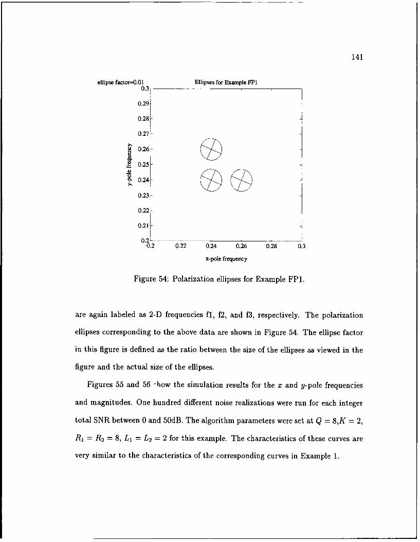
141
ellipse factorff0.01 Ellipses for Example FPI0.3
0.29
0.28
0.27
: 0.26
0.25
0.25 I0.23-
0.22
0.21
0.2_ __ i0.2 0.22 0.24 0.26 0.28 0.3
x-pole frequency
Figure 54: Polarization ellipses for Example FP1.
are again labeled as 2-D frequencies fl, f2, and f3, respectively. The polarization
ellipses corresponding to the above data are shown in Figure 54. The ellipse factor
in this figure is defined as the ratio between the size of the ellipses as viewed in the
figure and the actual size of the ellipses.
Figures 55 and 56 -how the simulation results for the x and y-pole frequencies
and magnitudes. One hundred different noise realizations were run for each integer
total SNR between 0 and 50dB. The algorithm parameters were set at Q = 8,K = 2,
R, = R2 = 8, L, = L2 = 2 for this example. The characteristics of these curves are
very similar to the characteristics of the corresponding curves in Example 1.
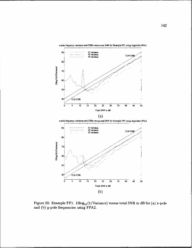
142
x-pole frequency variances and CRBs versus total SNR for Example Fpl using Algorithm FPA2
90- ---------------- fl variance-- - - - f2 variance 0.24 CR
B3 variance
60
0 5 10 15 20 25 30 35 40 45 50
Total SNR In dB
(a)y-pole frequency variances and CRBs versus total SNR for Example FP1 using Algorithm FPA2
90 - -------- fl variance--------- f2 variance0.4C P - ,03 variance0.4RX -
80 i ;f70-
ce60 . *' %0
50
40 20 25 0 5
0 5 10 15 20 25 30 35 40 45 50
Total SNR indB
(b)
Figure 55: Example FP1. 101ogl 0 (1/Variance) versus total SNR in dB for (a) x-poleand (b) y-pole frequencies using FPA2.
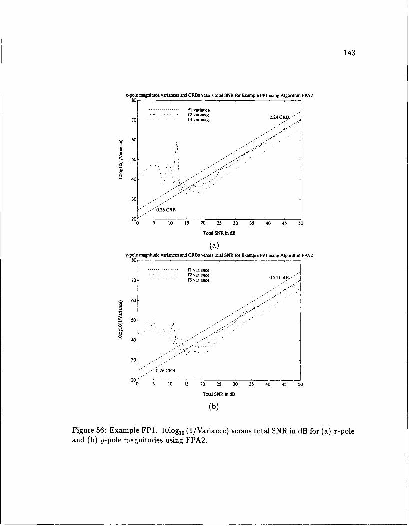
143
x-pole magnitude variances and CRBs versus total SNR for Example MP using Algorithim FPA2801
I----- ----- ---- fl. variance--------- f2 variance0.4C
70- --- - 0 variance0.C
z 60
50- 5 1 S 2 5 3 5 4 5 5
%oa N nd
4(a)
0.2 vaincR.2BR
60 L
0 -' 5 2 5 3 5 4 5 5
40-
60-x
30-
0.26 CRB20
0 5 10 15 20 25 30 35 40 45 50
Total SNR in dB
(b)
Figure 56: Example FP1. 101ogl0 (1/Variance) versus total SNR in dB for (a) x-poleand (b) y-pole magnitudes using FPA2.
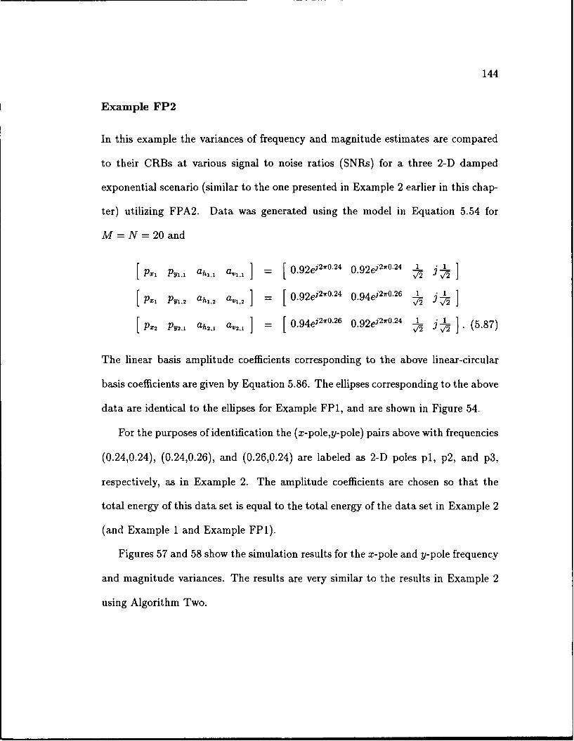
144
Example FP2
In this example the variances of frequency and magnitude estimates are compared
to their CRBs at various signal to noise ratios (SNRs) for a three 2-D damped
exponential scenario (similar to the one presented in Example 2 earlier in this chap-
ter) utilizing FPA2. Data was generated using the model in Equation 5.54 for
M = N = 20 and
[x p,,1 p,, ahl, al, 0 .92e j2 wO24 0.92e j2x0 24 1 j_ ]PX1 pY12 ahl,2 avl,2 0 .92e j2w.2 4 0.94e j2wx26 1 I_
[P2:2 PY2, ah2,, a,,21 0 .94e j2wO26 O.92ej2w10 24 I j~ _L 5.7
The linear basis amplitude coefficients corresponding to the above linear-circular
basis coefficients are given by Equation 5.86. The ellipses corresponding to the above
data are identical to the ellipses for Example FP1, and are shown in Figure 54.
For the purposes of identification the (x-pole,y-pole) pairs above with frequencies
(0.24,0.24), (0.24,0.26), and (0.26,0.24) are labeled as 2-D poles pl, p2, and p3,
respectively, as in Example 2. The amplitude coefficients are chosen so that the
total energy of this data set is equal to the total energy of the data set in Example 2
(and Example 1 and Example FP1).
Figures 57 and 58 show the simulation results for the x-pole and y-pole frequency
and magnitude variances. The results are very similar to the results in Example 2
using Algorithm Two.
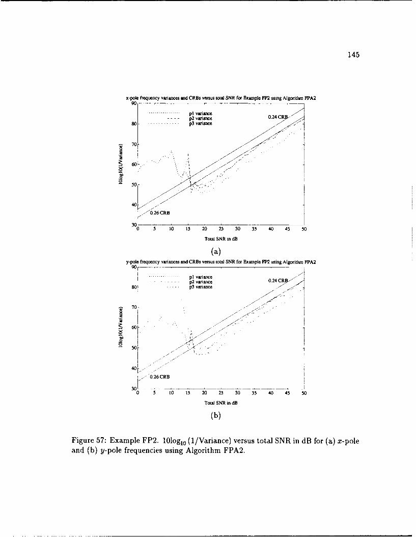
145
x-pole frequency variances and CRBs versus total SNR for Example FP2 using Algorithm FPA290
--- --- --- --- pi variance----- p2variance 0.24 CRP -
80 .. ... p3 variance
70-
50-'.
40
~26 CRB
3010 5 10 15 20 25 30 35 40 45 50
Total SNR in dIB
(a)y-pole frequency variances and CR~s versus total SNR for Example FP2 using Algorithm FPA2
90,
---- - --- p1 variance0.4C )-8 p2 variance 02C~8--- p3 variance --
70k
.22CR
30 - - ---- to 5 0 3 3 4 4_5
Total SNR mn dB
(b)
Figure 57: Example FP2. 101ogl0 (1/Variance) versus total SNR in dB for (a) x-poleand (b) y-pole frequencies using Algorithm FPA2.
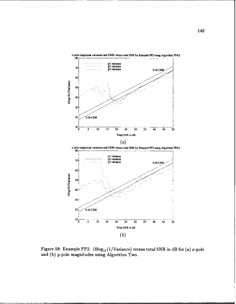
146
x-pole magnitude variances and CRBs versus total SNR for Example FP2 using Algorithm FPA280
- ---------p l v a r a n c
..pl magn ...ude variances an0.svru oalSRfrEapeF 24 sn Ar itmB
60-
j50-
~40 .
30-~-
20 - 0.26 CRB
100 5 10 15 20 25 30 35 40 45 50
Total SNR in dB
(a)
ad() y-pole magnitudesvracsadC~ ess oa N o xml P using Algorithm Two.
147
5.4 Summary
In this chapter the 2-D TLS-Prony Technique was developed. This is a new tech-
nique for estimating two-dimensional (2-D) poles and amplitude coefficients in a
2-D Prony-based model. The fundamental estimation algorithm (Algorithm One)
involves two parts, each utilizing a 1-D singular value decomposition-based tech-
nique, and is capable of locating frequencies anywhere in the 2-D frequency plane.
The basic algorithm was first developed for a single 2-D data set, such as a set
of radar measurements with a single transmit ard receive polarization. Simula-
tions were shown which demonstrate the performance of the algorithm for various
noise levels. Then, the algorithm was extended to the full-polarization case which
requires full-polarization 2-D measurements of a target. Simulations were shown
which demonstrate the performance of this algorithm for various noise levels. The
performance characteristics for both the single-polarization and full-polarization al-
gorithms are shown to be nearly identical.
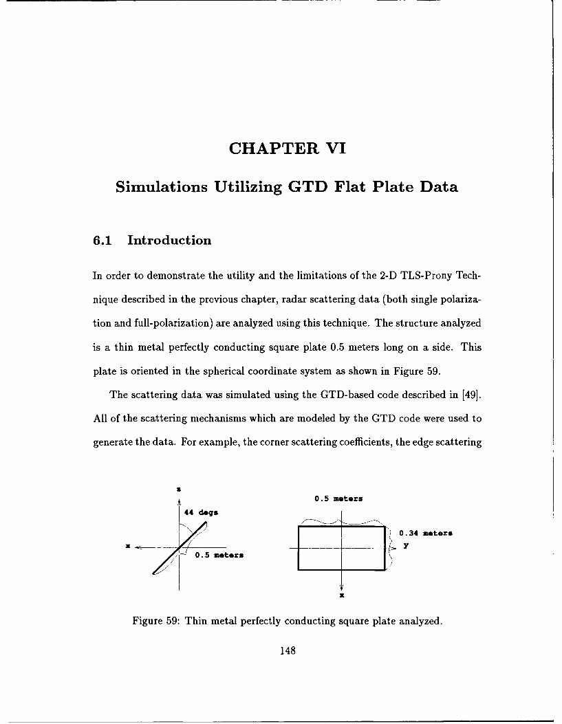
CHAPTER VI
Simulations Utilizing GTD Flat Plate Data
6.1 Introduction
In order to demonstrate the utility and the limitations of the 2-D TLS-Prony Tech-
nique described in the previous chapter, radar scattering data (both single polariza-
tion and full-polarization) are analyzed using this technique. The structure analyzed
is a thin metal perfectly conducting square plate 0.5 meters long on a side. This
plate is oriented in the spherical coordinate system as shown in Figure 59.
The scattering data was simulated using the GTD-based code described in [49].
All of the scattering mechanisms which are modeled by the GTD code were used to
generate the data. For example, the corner scattering coefficients, the edge scattering
0.5 meters
44 dogs
0.34 meters
0.5 meters
Figure 59: Thin metal perfectly conducting square plate analyzed.
148
149
coefficients and the double-bounce coefficients are included in the data set. However,
the corner scattering coefficients are the dominant terms in the data.
The locations, damping factors and polarimetric properties of the scattering
centers which exist on the plate are estimated using both the single-polarization
TLS-Prony Technique and the full-polarization TLS-Prony Technique. This struc-
ture contains corners and edges at both grazing and non-grazing angles. Thus,
the abilities of the 2-D TLS-Prony Technique to estimate non-point scatterer type
scattering centers is demonstrated.
The examples that are shown in this chapter are intended to investigate several
issues. First, the quality of the parameter estimates as a function of 2-D angular
and frequency bandwidth is demonstrated. Limited angular data sets over several
2-D angular and frequency bandwidths are analyzed in this chapter. Second, the
ability of the estimation algorithms to use data directly in polar form, rather than
interpolating the data onto a rectangular data grid in the 2-D frequency plane, is
investigated. Third, the effects of noise on the parameter estimates for the various
data sets is examined. Also, the effects (on the parameter estimates) of choosing
model orders which are equal to and greater than the expected number of scattering
centers are examined.
Recall that the 2-D TLS-Prony Technique requires data on a rectangular grid
in the 2-D frequency plane. However, if the data (gathered by a radar) lies on a
polar grid, it is possible to treat this data as if it lies on a rectangular grid if the
polar grid is over a relatively small angular bandwidth (usually under 150) and the
150
center frequency is larger than several times the frequency bandwidth of the data.
Thus, the polar data is assumed to lie directly on a rectangular (or square) grid. A
polar data set over a 150 angular swath with a center frequency to bandwidth ratio
of 4.029 is utilized directly as the data in the 2-D TLS-Prony Technique. Then this
data set is interpolated onto a square data grid and the results of the two sets of
simulations are compared. Another polar data set over a 30 angular swath is also
analyzed. The polar data over this angular swath is also directly utilized by the
2-D TLS-Prony Technique, but in this case the center frequency to bandwidth ratio
is 19.250. The interpolation of this 30 onto a square grid is not examined in detail
since the polar grid closely resembles the square grid for such a small 2-D angular
and frequency bandwidth.
Most of the examples shown involve scenarios where no noise is added to the
scattering data. The effects of noise on the parameter estimates are demonstrated
by considering the relative error (RE) versus total SNR for the various data sets. It
is shown that for two of the thr-e data sets examined, the RE and thus the parameter
estimates are not effected by noise for total SNRs over 15 dB. The single data set
which yields parameter estimates which are effected by noise for SNRs up to and over
50 dB is the polar data set over a 30 angular swath. This data set is more sensitive to
noise since the resolution (in the 2-D range domain) is the smallest of all of the data
sets (due to the fact that the 2-D angular and frequency bandwidths are the smallest
for this data set). The 2-D TLS-Prony Technique is superresolving the scattering
centers, and the parameter estimates are more sensitive to noise. It is demonstrated
151
in [10] that the parameter estimates associated with various parametric techniques,
such as Prony's Method, are sensitive to noise when the parametric techniques are
superresolving modes. The effects of noise for the 3' polar swath data are shown in
the form of scatter plots for scattering center locations for various total SNRs.
6.2 Description of Data
The first data set analyzed consists of the monostatic scattering matrix from the
plate for incidence angles of -7.5' < 0 < 97.5' with 9 fixed at 900. The frequency
range is from 9 GHz to 11.55 GHZ in 0.085 GHz steps. The angular step size is
0.5'. Thus, the data set is 31x211 (number of frequencies x number of angles).
Data segments of size 31 x 31 are analyzed using Algorithm Two and FPA2. This
corresponds to a 15' polar swath of data. The unambiguous range for this data set
is 1.7637 meters in each direction. Note that this data, which lies on the polar grid,
is used directly by the 2-D TLS-Prony Technique, without being interpolated onto
a square grid. Recall that the 2-D TLS-Prony Technique requires data which lies
on a rectangular grid in the 2-D frequency plane. Thus, it is assumed that since
these polar data sets are over a relatively small angular swath (15') and the center
frequency is 4.029 times the bandwidth, it is a reasonable approximation to assume
that the polar grid is close enough to a square grid to treat the data as if it lies on a
square grid. The frequency and angular step sizes of 0.085 GHz and 0.5' were chosen
to make the spacing in the frequency direction very close to the spacing between
data samples in the angular direction on the 2-D frequency plane. This validity of
this assumption is investigated in the examples which utilize this data set, which is
152
designated the 150 polar swath of data.
The second data set analyzed consists of several 29 x 29 data segments which lie
on a square grid in the 2-D frequency plane. These data sets were interpolated from
the 150 polar swaths of data segments. Twenty-seven different square grid data sets
are interpolated from the 150 polar swaths of data. There are nine different center
angles for the square grid data sets, and three polarizations per center angle. The
interpolation method in Equation 4.27 was used to interpolate the 31 x31 15' polar
swath data sets to the 29 x 29 square grid data sets. The spacing between the square
grid data points is 0.085 GHz in each direction on the 2-D frequency plane. The
reason that the square grid is only 29x29 while tie polar grid is 31x31 is that by
making the square grid fit entirely within the polar grid, the need to extrapolate to
square grid data points which lie outside of the original polar grid is avoided.
The third data set analyzed consists of several 30 polar swaths of data. The
frequency range is from 9 GHz to 9.48 GHz in 0.016 GHz steps. The angular range
is ±1.5' around the center angle in 0.1' steps. Thus, these data sets are also of
size 31x31 points. The unambiguous range for these data sets is 9.3684 meters *,I
each direction. These 30 polar data sets are utilized directly by the 2-D TLS-Prony
Technique in polar form. Since this data set is over a very small angular swath (30)
and the center frequency is 19.250 times the bandwidth, it is a good approximation
to assume that the polar grid is close enough to a square grid to treat the data as
if it lies on a square grid. This is a much safer assumption than that made for the
150 polar swath of data. Results for scenarios where this 30 data is interpolated
153
onto a square grid as the 150 data are not shown since the polar grid is such a close
approximation to the square grid. Several sets of this 30 polar data were interpolated
onto a square grid and the results obtained (which are not shown) were, in general,
worse in a relative error sense to the results obtained using the polar data directly.
This is most probably due to the interpolation error which was introduced in the
interpolation step. The interpolation method is a linear function, and this is not an
accurate model for this data. The development of a more appropriate interpolation
technique is an area for future research.
The measurement geometry is shown in Figure 60. The four corners of the plate
are labeled C1, C2, C3, C4 in this figure. The projection of the plate onto the
xy-plane is the expected form of the image for all of the data sets since the slice of
data obtained is always limited to 0 = 90' (or the xy-plane). The angle 0 in this
figure is designated the center angle of rotation of the data. The data collected in
the 2-D frequency plane is depicted in Figure 61. First, a single-polarization TLS-
Prony algorithm (Algorithm Two) is applied to the data. Then, a full-polarization
TLS-Prony algorithm (FPA2) is applied to the data.
6.3 Single-Polarization Analysis of Plate
Figure 62 shows a contour image of the plate obtained by directly taking a 2-D IFFT
of the hh-polarization 15' polar swath of data and then re-scaling the axes. The
15' sector of data used was for azimuth angles of 37.50 < € _< 52.5'. The outline
of the plate corresponds to a plate at the center of this azimuth sweep, € = 45' .
The corners of the plate, labeled Cl, C2, C3, C4 in this figure correspond to the
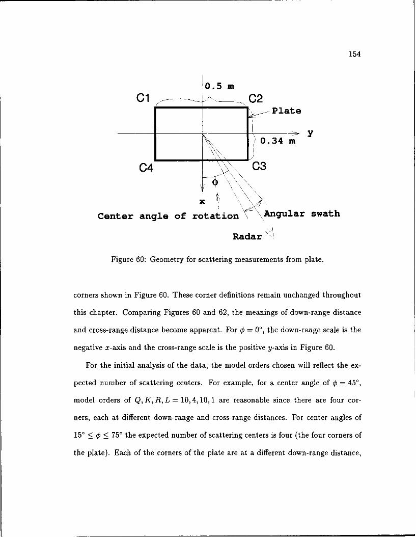
154
0.5 mC1C2
rJ Plate
/0.34 m
C4 1 C3
/ ,\ "' \ \\
Center angle of rotation \Angular swath
Radar
Figure 60: Geometry for scattering measurements from plate.
corners shown in Figure 60. These corner definitions remain unchanged throughout
this chapter. Comparing Figures 60 and 62, the meanings of down-range distance
and cross-range distance become apparent. For 0 = 00, the down-range scale is the
negative x-axis and the cross-range scale is the positive y-axis in Figure 60.
For the initial analysis of the data, the model orders chosen will reflect the ex-
pected number of scattering centers. For example, for a center angle of 0 = 450,
model orders of Q, K, R, L = 10, 4, 10, 1 are reasonable since there are four cor-
ners, each at different down-range and cross-range distances. For center angles of
15' < 0 < 750 the expected number of scattering centers is four (the four corners of
the plate). Each of the corners of the plate are at a different down-range distance,
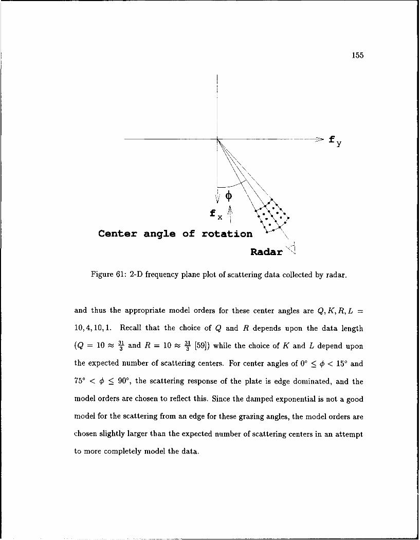
155
fY
A\
0 0
Center angle of rotation
Radar
Figure 61: 2-D frequency plane plot of scattering data collected by radar.
and thus the appropriate model orders for these center angles are Q, K, R, L =
10,4, 10,1. Recall that the choice of Q and R depends upon the data length
(Q = 10 - 3 and R = 10 - - [591) while the choice of K and L depend upon33
the expected number of scattering centers. For center angles of 0' < < 150 and
75' < 0 90', the scattering response of the plate is edge dominated, and the
model orders are chosen to reflect this. Since the damped exponential is not a good
model for the scattering from an edge for these grazing angles, the model orders are
chosen slightly larger than the expected number of scattering centers in an attempt
to more completely model the data.
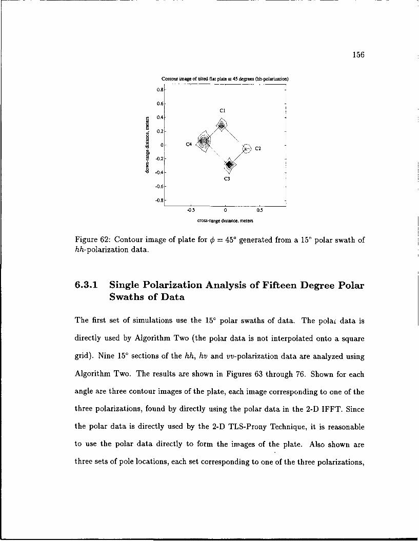
156
Contour image of tilted flat plate at 45 degrees (hh-polarizanon)
0.8
0.6CI
0.4-I
0.2-
0 C4;El, C2
-0.2
"v -0.4-
C3
-0.6
-0.8
-0.5 0 0.5
cross-range distance, meters
Figure 62: Contour image of plate for € = 450 generated from a 150 polar swath ofhh-polarization data.
6.3.1 Single Polarization Analysis of Fifteen Degree PolarSwaths of Data
The first set of simulations use the 15' polar swaths of data. The polar data is
directly used by Algorithm Two (the polar data is not interpolated onto a square
grid). Nine 150 sections of the hh, hv and vv-polarization data are analyzed using
Algorithm Two. The results are shown in Figures 63 through 76. Shown for each
angle are three contour images of the plate, each image corresponding to one of the
three polarizations, found by directly using the polar data in the 2-D IFFT. Since
the polar data is directly used by the 2-D TLS-Prony Technique, it is reasonable
to use the polar data directly to form the images of the plate. Also shown are
three sets of pole locations, each set corresponding to one of the three polarizations,
157
estimated by Algorithm Two with no noise added to the original data. In the cases
where there are more than four poles, only the four highest energy poles are shown
in these plots.
Along with these plots are shown contour images which were generated from the
estimated parameters. The parameters estimated by Algorithm Two are used in
the 2-D model in Equation 5.2 to generate data in the 2-D frequency domain. Note
that all of the parameters estimated by Algorithm Two are used to generate this
data (not just the four highest energy poles). This data is then transformed into
the image domain and the results are shown in the figures. Outlines of the plate are
shown for the center of the azimuth sweep. The data used to generate each contour
image is a 31 x 31 data set, where the angular data was taken at ±7.5' around
the angle indicated, which is the center of the rotation. For each plot, the entire
unambiguous range is shown which is 1.7637 meters in each direction.
It must be pointed out that all of the contour images shown in this chapter, in
general, are on different magnitude scales. That is, the value of a given contour
line for one contour plot is not necessarily the same value on another contour plot.
Thus, the contour plots are shown to demonstrate the form of each individual im-
age, and relative magnitude comparisons between images can not be made. The
differences between an original data generated contour image and its corresponding
model generated contour image are reflected in the relative error (RE) between the
two images, which is defined in Equation 6.1. It also must be emphasized that an
outline of the plate (projected onto the xy-plane) is sketched in most plots shown in
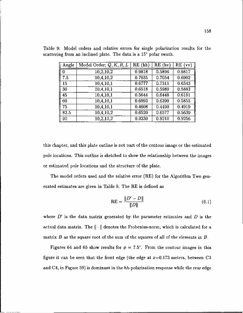
158
Table 9: Model orders and relative errors for single polarization results for thescattering from an inclined plate. The data is a 150 polar swath.
[j Angle ] Model Order; Q, K, R, L RE (hh) RE (hv) RE (vv)
0 10,2,10,2 0.9818 0.5896 0.98177.5 10,4,10,2 0.7035 0.7054 0.690215 10,4,10,1 0.6777 0.7311 0.634330 10,4,10,1 0.6518 0.5989 0.588345 10,4,10,1 0.5644 0.6448 0.619160 10,4,10,1 0.6993 0.6390 0.585575 10,4,10,1 0.4608 0.4490 0.491982.5 10,4,10,2 0.6520 0.6577 0.563990 10,2,10,2 0.9230 0.9210 0.9256
this chapter, and this plate outline is not Dart of the contour image or the estimated
pole locations. This outline is sketched to show the relationship between the images
or estimated pole locations and the structure of the plate.
The model orders used and the relative error (RE) for the Algorithm Two gen-
erated estimates are given in Table 9. The RE is defined as
RE- ID'- DII (6.1)
IIDII
where D' is the data matrix generated by the parameter estimates and D is the
actual data matrix. The 11. 1 denotes the Frobenius-norm, which is calculated for a
matrix B as the square root of the sum of the squares of all of the elements in B.
Figures 64 and 65 show results for k = 7.5' . From the contour images in this
figure it can be seen that the front edge (the edge at x=0.173 meters, between C3
and C4, in Figure 59) is dominant in the hh-polarization response while the rear edge
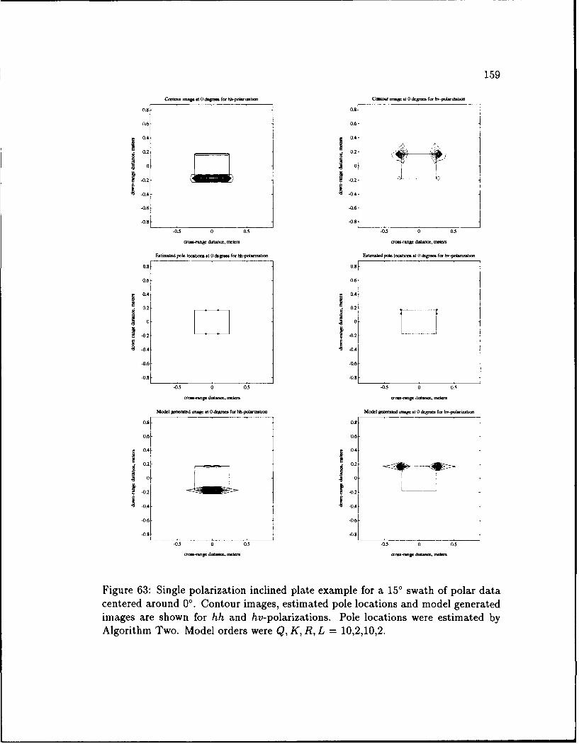
159
Cata" m'ap¢ at 0 deg for hh-polanm C-t-~ a'nW at 0 dg for h-paw= m
0.6 06
0.4 0 i
0.2 _- 0.2[ >- ."
0
-0.2 -U 0.2 5 0.
04 -10.4
-0.6-1 -0.6
-0.5 0 0.5 -5 0 05S
¢'am-,tang dut- , met- g db- momcn
EstMt.ed pok IObUo1 .t 0 &g- fo hh-po4.noabon Etmsd p. Io.tlmw a 0 1gro.. fo. ho-pkn9-
0.8 0.8
0.6- 0.6-
0.4-j 0.4-1
-0.2 - 0.2
-0.4 -0.4-0.6 -0.6
-0.8 -0.9
-0.5 0 05 -0.5 0 05
a-Mge dulta .mn srm. dgww ., mtm.
Mo&l 3,ao..1.d .mage t 0 &qm f. hh-pol.I.. Mode gc Wo.d oll3W t1 0 & fo hf-po.loobo
0.8- 0.8-
0.6- 0.6
1! 0.4- 0.4
I:10. .
-0.2- -0.24
.0.4 .0.4 -
-0.6 -06 k
0.8 -0.8
-0.5 0 0.5 -0 0 0.5
Figure 63: Single polarization inclined plate example for a 150 swath of polar datacentered around 0'. Contour images, estimated pole locations and model generatedimages are shown for hh and hv-polarizations. Pole locations were estimated byAlgorithm Two. Model orders were Q, K, R, L = 10,2,10,2.
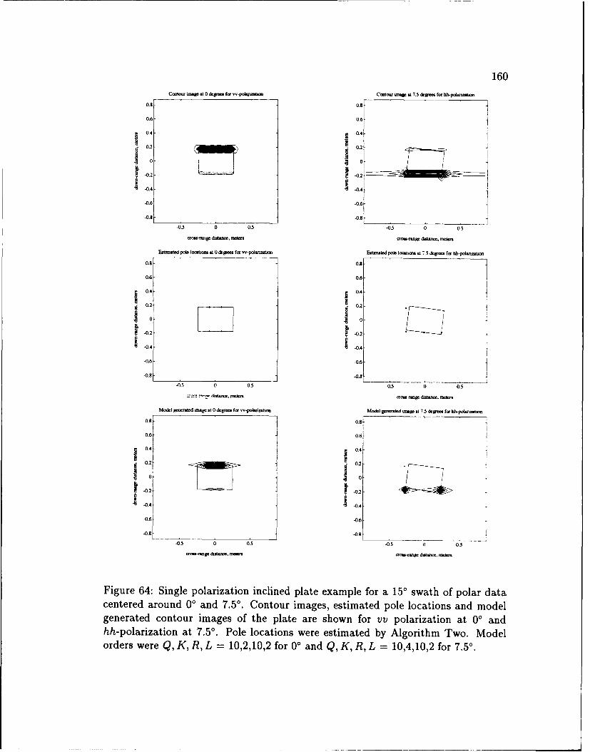
160Cotour m..ge at0 degrees for -- olrno Csci,r at 7.5 degree for Whpolrmnae
0.6- 0-6
I0.4 0.4
0.2 0.2
00
-0.2 -0.2-
-0.4- -0.4-
-0.68 -0.6 -
-0-5 0 0 .5 -0.5 0 0.1
ao-rage dwatnce, meters oro-rnge dmsluna, meters
Estimated pole locatin at0 dlepees for vv-plarnatom Estimated Pole Iocstios .t 7.5 dere fo 5 pjo
0.8- 0.8-
0.6- 0.6-
0.4- 0.4-
0. 0.I- --
0.2 -0.2
S-0.4 1-0.4-0.6 -0.6
-0.8 A0.
-0.5 0 0.5 -050 0.5
-dotanoe' m stg du.1.na trien,
Model generaed image at 0 dcgeea. for v-polarization Mock] generated ie at 7.5 degrees for til.omnam
0.8 - 0.8-- ---- -- -----
0.6- 0.6f
0.4- 0.4
0.20.
100
-0.2 L .J.0.2
-0.8- -089
-0.5 0 0.5 -0.5 0 ~
Figure 64: Single polarization inclined plate example for a 15' swath of polar datacentered around 00 and 7.5'. Contour images, estimated pole locations and modelgenerated contour images of the plate are shown for vv polarization at 00 andhh-polarization at 7.5'. Pole locations were estimated by Algorithm Two. Modelorders were Q, K, R, L = 10,2,10,2 for 00 and Q, K, R, L = 10,4,10,2 for 7.5'.
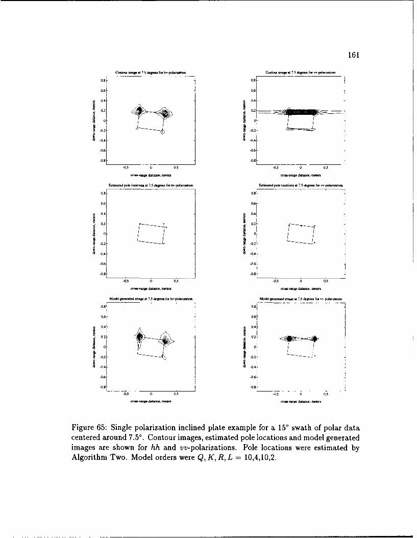
161
Comtog uuge at 7.5 dege for hv-poiaruat Cwtou'r wW St 7.5 d'pe fo -pol
-o n
0.8- 0.8
0.6- 0.6-
0.4- 0.4
0.2- 0.
-0.2 - - j>-02
-0.4-0
-0.'6 -0.-
-0.8 -0.8
-05 0 0,5 -03 0 0.5
a-rlg. diltance, reters r5-g.an dLdac me,
Estimated pole locatfiow at 7.5 degrem for h-pm-zaon Estmate pole Ioclostr at 7.5 deges for w-pok-to
0.8 0.8
0.6 0.6
0.4 0.4
0.2 0.2
10 10
S-0.2 -0.2
-0.4 -0.4-
-0.6 -0.6
-0,5 0 0.5 -0.5 0 0.5
orW d-an distantc, mote. man-sF dta nce.m
Model gomerted mage at 7-5 dogma for hv-polalmmtim Model gornated map at 7.5 d gres for ,.-pormoaxmm
0.8 0.8-
0.6 0.6
0.42 041.
0; 0-0.2- -0.24
-0.6
-0.8 -0.8
-05 0 0.5 -05 0 0.
~-nodwsam. mom oe-maP d.stmo moms
Figure 65: Single polarization inclined plate example for a 150 swath of polar datacentered around 7.5'. Contour images, estimated pole locations and model generatedimages are shown for hh and vv-polarizations. Pole locations were estimated byAlgorithm Two. Model orders were Q, K, R, L = 10,4,10,2.
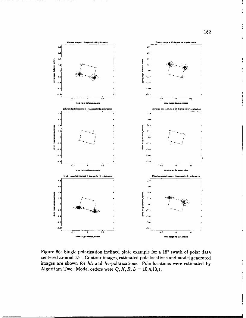
162
CQptonw am~ .15 f fp. hh-pohn.bm Ctm at. .15 dmp fm bv-polnt.bw
0.83 0.8-
0.6- 0.6-
0.4- 0.4
0.2 0.2
10 10-0.2 -012
-0.4- -0.4
-0.6- -0.6
-0.5 0 0.5 -0.5 0 0.5
0.8- 0.8-
0.6- 0.6-
0.4- 0.4-
0.2 0.2-
0 0-
-0.2-02
I -0.4-- -0.4
-0.6- -0.6-
-0.8- -0.8-0.5 0 0.5 -0.5 0 0.5
0.8- 0.98
0.6- 0.6-
0.4- 0.4-
0.2 0-2
10 10-
S-0.2 ~-0.2I -0.4-1 -0.4
-0.6- -0.6
-0.8 -- 08.-0.5 0 0.5 -0.5 0 0.5
Figure 66: Single polarization inclined plate example for a 150 swath of polar datacentered around 150. Contour images, estimated pole locations and model generatedimages are shown for hh and hv-polarizations. Pole locations were estimated byAlgorithm Two. Model orders were Q, K, R, L = 10,4,10,1.
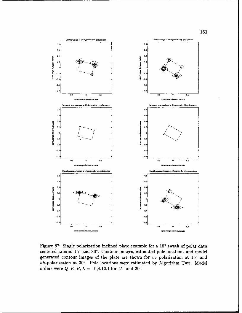
163Ctot. .au at 15 t.gr for w-vpolamnon Cto W at 30 degre. for hh-poh-1mon
0.8 0.8
0.6 0.6
0.4 0.4
0.2 02
10 ~0 &
0.2 .0.2
.0.4 -0.4
-0.6 -06
-0.8 -0.8
-0.5 0 0.5 -0.5 0 0.5
.cange diatenc, nrcm os-ange duammrnee,
Etmmted pole locabos at 15 degre fs vvfpolrml-on Emgtated pcle Iocabons at 30 dg for hh-polfr~tm
0.8 0.8
0.6 0.6
0.4- 0.4-
0.2 - 0.2
-0.28 -0.2
-0.4 -0.4
-0.620.
-0.4 -0411
-0.5 0 05 -0.5 0 0-5
ro-llge dislWan, mcter. S-ge Anan, Me.ea
Model generated umage at 15 degrees for vv-polarmtimO Model ge.ated unar at 30 deree. for hh-pol-rizmtan
0.8 0.8-
0.6 0.6
0.4- 0.4-
• 0. -, -0 0
-0.2 .0.2
-0.4 -0.64
-0.8 -0.8
-0.5 0 05 -0.5 0 0.5
ero-rnge delance, me.. am-g. di.e l.Wlen
Figure 67: Single polarization inclined plate example for a 150 swath of polar datacentered around 15' and 30'. Contour images, estimated pole locations and modelgenerated contour images of the plate are shown for vv polarization at 15' andhh-polarization at 30'. Pole locations were estimated by Algorithm Two. Modelorders were Q, K, R, L = 10,4,10,1 for 150 and 300.

164
Contol. uap at 30 degfs for hv-pol-izotian C-ota- t nap t 30 d.. foe -.pol.oallll
0.8 0.8
0.6 0.6
0.4,j 0.4
0. 0
-0.2 0.2-0.4 -0.
-0.6 -0.6
-0.8 -0.8
.0.5 0 0.5 -0-5 0 0.5
oi-rSge ddee, meta.s erna-1at dtame, melAM
Elmmied pole Ioittoes t 130 degee. foe hv-polareboe Esnimaled pole locmms at 30 degseea . .
0.8 0.8
0.6 0.6
0.2- 0.2 -
0.4- 0.4
. -0.2 - 0.2
S.0.4 0.4
-0.6 -0.6
-0.8 -0.8
.0.5 0 0.5 -0.5 0 0.5
m.-gnge dwArmm, meters -ange dtmnc, eu
Model geearted irmage at 30 degree fo hv-pohminlcm Model geoeested una at 30 degrees for v-polarm tmn
0.8 0.
0.6 0.6-
0.4-04
0.2 ~.0.20 0
0.2 I0.2
-0.6 -0.6
-0.8 -0.8
-0.5 0 0.5 0.5 0 0.5
ar.--gog dainor, meter ea- ge d-.oe.
Figure 68: Single polarization inclined plate example for a 150 swath of polar datacentered around 30'. Contour images, estimated pole locations and model generatedimages are shown for hh and hv-polarizations. Pole locations were estimated byAlgorithm Two. Model orders were Q, K, R, L = 10,4,10,1.
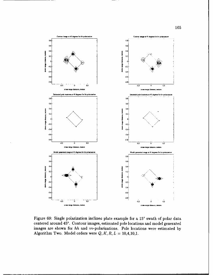
165
Contoor mWS a 45 dg-o. fto hh-polanrbon Cotor -W .145 dcg-. f h -p.nol-o
0.8- 0.8
0.6 0.6
0.4- 0.4-
0.2 028 8 0
0.2 . -0.2 .1
-0.6 -0.6-
-0.8 -0.8
-0.5 0 0.5 -0.5 0 03
crm~l-tge dw mc, mete..n c--m. dw-, .w.
rstim ted pole Ioot 145 d=esgra fo hh-pohoeaomt E10-tod polo ob-oo. M 45 g g fo h -pol.,oobo
0.8 0.8
0.6 0.6
0.4- 0.4
0.2 0.2 / \
0 /
-0.2 -0.2
-0.4- 44.4
0.6 -0.6
-0.8 -0.8
-0,5 0 0.5 -0.5 0 0.5
rc-ra-ge dzt- , -I.. -~c-g. d.1-ma-
Model g aeted onge at 45 dego fo hh-poioonfim Model go.nbId -mVu .145 dg-o.. fo hb-p.trmmto
0.8 0.8-
0.6 0.6-
0.4 A 0.4-
0.2 0.2 /
0 .9 . 0-
.0.2 -0.2
-0.6 -0.6
-0.8 -0.8
-0.5 0 0.5 -0.5 0 0-5
d-w-ra ¢ddne. mate ro-r-ge dw-, wtm
Figure 69: Single polarization inclined plate example for a 150 swath of polar datacentered around 45'. Contour images, estimated pole locations and model generatedimages are shown for hh and vv-polarizations. Pole locations were estimated byAlgorithm Two. Model orders were Q, K, R, L = 10,4,10,1.
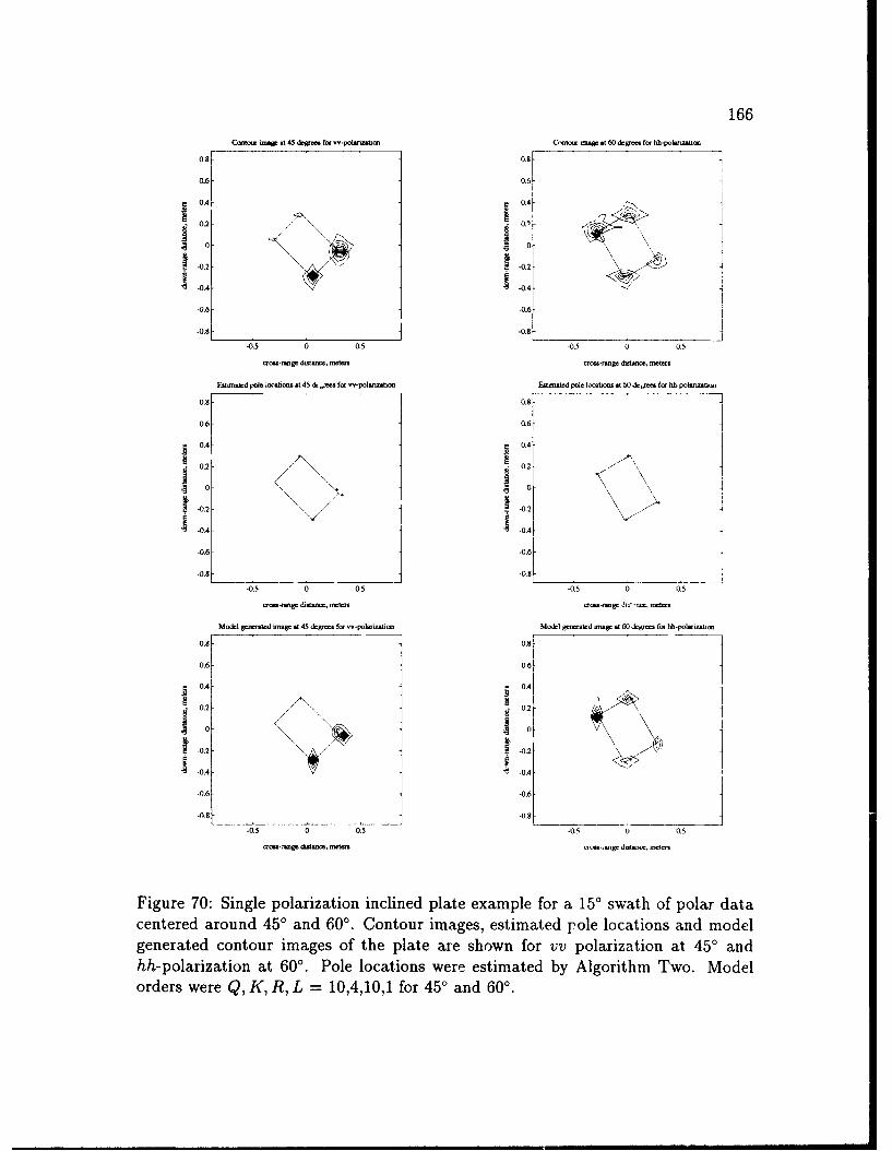
166Contm map at 45 dogis for -polanza umr C,"tio.* m.a .160 egOro. for hh-poL""Um
0.8- 0.8
0.6- 06
0.4 04
0.2 / 0100 40
0 .04 -0.4-0.6 -0.6
0.6- -0.6
-0.5 0 05 -0.5 0 0.5
a.roanmgr droanoe, meters crmo-r~oge d..oo.n.000
E,tMld polo 1ocatios at 45 &,o. for w-polnMAton Esrmsatod polo Ic-abtc .160 &coro. for hh-poh-Unton
0.8- 0.8
0.6 0.6
0.4 0.4
0.2 0.2 ,
-0.2 1-0.2-
-0.6- -0.6
-0.8 -0.8-0.5 0 0.5 -0.5 0 05
ooc -oogo di.1aoomotonelrs co -rmn8 .'-nor, rn.1000
Model geortated mago at 45 dg-gr. fom w-porizmtiom ModI g-moated -mag at 60 dgrs fo hh-pol-rmtot
0.8 0.8
0. 0,6-
0.4 - 0.4
-0.2 0.2I
-0.2 -0
.
-0.4 -0.4
-0.6 -0.6
-0.8 -0.8
-0.5 0 0.5 -0.5 0 05
--o -.000g. dtmmy, moor aoro ng dottaoor, motor.
Figure 70: Single polarization inclined plate example for a 150 swath of polar datacentered around 450 and 600. Contour images, estimated pole locations and modelgenerated contour images of the plate are shown for vv polarization at 450 andhh-polarization at 600. Pole locations were estimated by Algorithm Two. Modelorders were Q, K, R, L = 10,4,10,1 for 450 and 600.
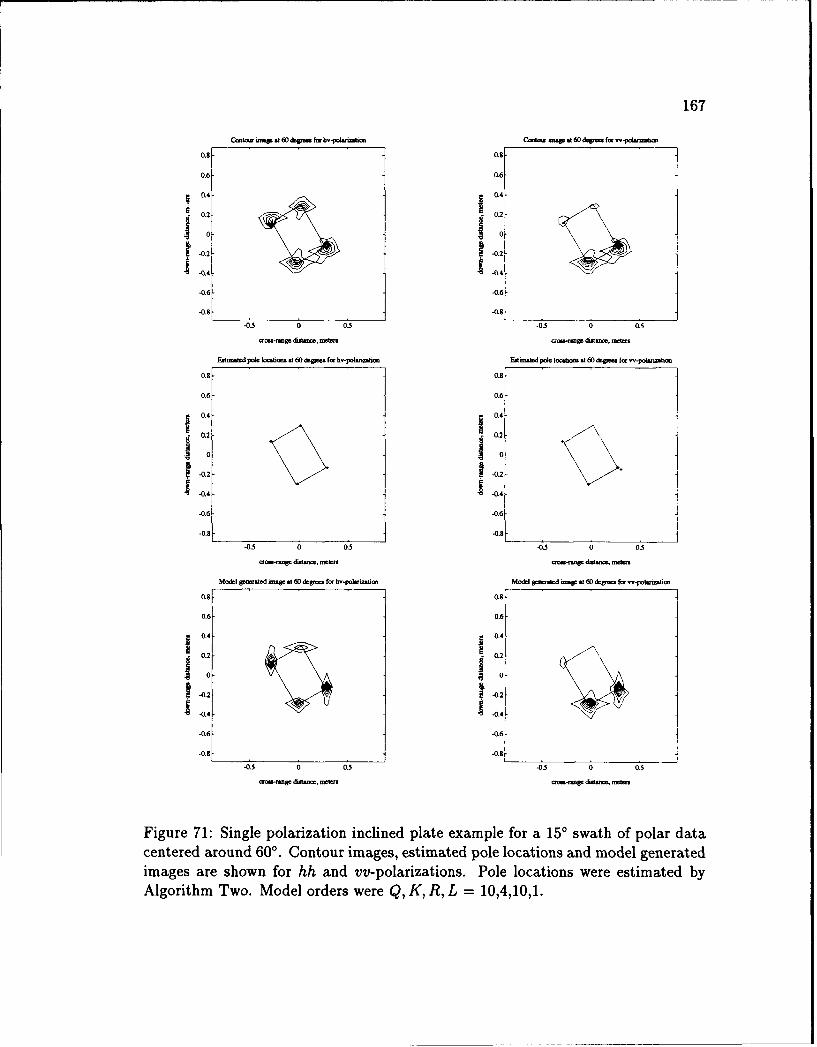
167
Ccmrw at~ 6*0 dsp... Ibr hvvOl~vmhc Cc-tma- t 6Od~s. k -polrn.mt
0.8- 0.8
0.6- 0.6-
0.4-__ 0.4-
0.2 02
-0.2 -0.2
-GA4 -0.4
-0.6 -0.6
-0.8 -0.81
-0.5 0 0.5 -0.5 0 0.5
Eotmated pole baosh..,. at 60 dtgnm for hv-poanimi Eebmtd pole locdasbat 6 0
degmes for v-pocwsbm
0.8- 0.8
0.6- 0.6
0.4- 04,
0 0-0.2 -0.2
I.0.4 -.4
-0.6 -0.6
-0.8 -0.8
-0.5 0 0.5 -0 . 0 0.5
Mdodel gimrted i...8. at 6 degree. fb. hv-polaizmm Model gp.er1.d imW st60 dep... for "-potanmfla
0.8 -0.8-
0.6- 0.6-
0.4-- 0.4-
I 02 - \-0.210 10
-0.2 -0.2
1-0.4 .04
-0.6- -0.6-
-0.- -0.8 ________________________________-0.5 0 0.5 -0.5 0 0.5
.a0Uasfl6. dmb-,. meters dmbw&..' mter
Figure 71: Single polarization inclined plate example for a 150 swath of polar datacentered around 600. Contour images, estimated pole locations and model generatedimages are shown for hh and vv-polarizations. Pole locations were estimated byAlgorithm Two. Model orders were Q, K, R, L = 10,4,10,1.
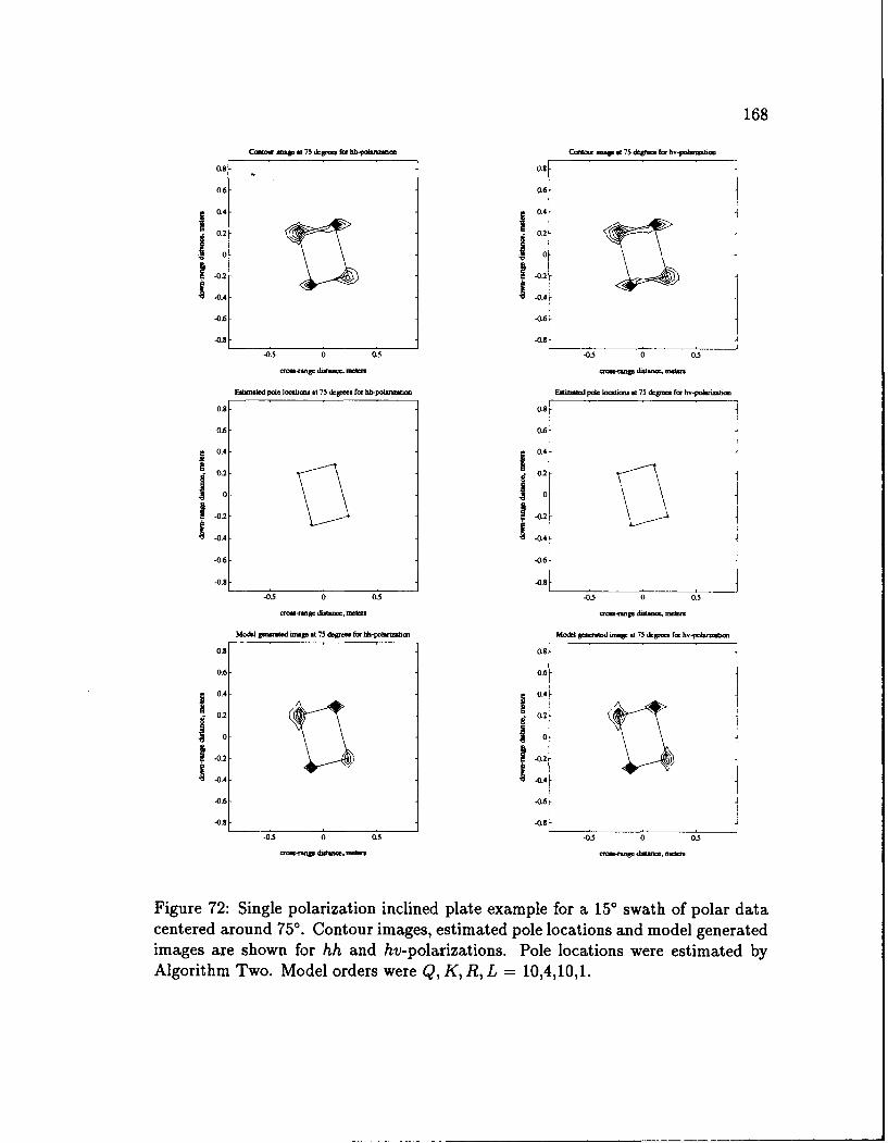
168
C tmf ns. at 75 6W= f. hh-poaruatt Cat= w in at 75 dses.. fm~ kv-poatm
o.g 0.8
0.6 0.6
0.4 0.4-
10.2 .2
0 0
-0.4-1 -024
-0.6 -0.6
-0.8 -0.O
-0.5 0 0.5 -03 0 0.5
rws-rage dtance, measa-wma ditata. s
Estunated pole lonoasa at 75 degices fm hh-pOaNUzabc Esttmad pA kxab at 75 dasa fmx hv-p o-i.mona
0.8 0.8
0.6 0.6
0.4- 0.4-
0.2
0- 0-
I -0.2-I -0.2-
1-0.4- -04-0.6 -0.6
-0.8 -0,8
-0.5 0 0.3 -0.5 0 0.5
Model geate id map at 75 dWma for hh-pohrmbat Model edma- at 75 dgr-.. fo hv-polatrmunt
0.8 0.8
0.6 0.6
0.4- 0.4-
I o I oI-0.2 I0.20 0
-0.4 1 -0.4
-.0.6 -0.6-0.8 -0.8
-0.5 0 0,5 -0.3 0 03
ratsWn dwta, fr aari duamme Mn
Figure 72: Single polarization inclined plate example for a 150 swath of polar datacentered around 75'. Contour images, estimated pole locations and model generatedimages are shown for hh and hv-polarizations. Pole locations were estimated byAlgorithm Two. Model orders were Q, K, R, L = 10,4,10,1.
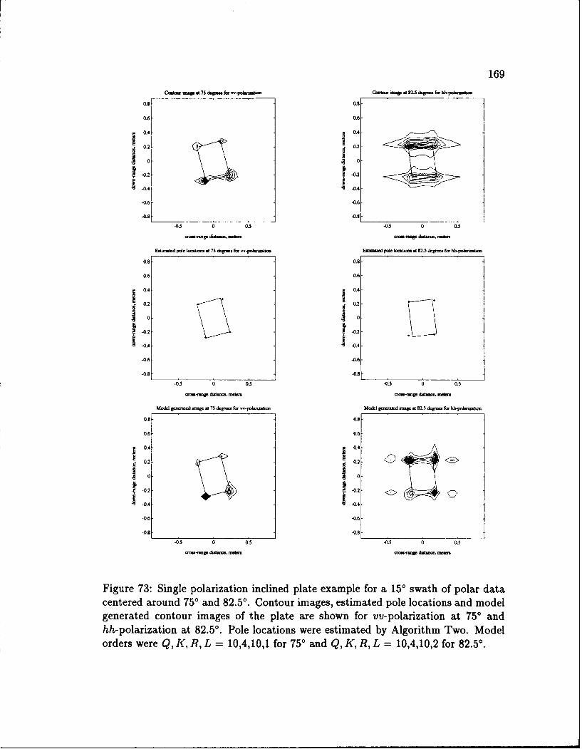
169
."p un a 75 d&p. for .- poharizauo Ca~mia at 82.5 dcua Ix thpola .
0.8 -0.8
0.6- 0.6-
0.4- 0.4-
10 10
-.2 -0.2
-.4 -.4
-0.6 -0.6
-09 -0.5 0 0.5 -. -0 .5 0 0.5 1
crow-rpeg do., um.Nn N-tWg d..tatoo tam
Edted pole loratto. at 75 dqgoor for vvpo~lmbon Etoitd pole tomuoa at 82.5 deg,.. for hh-pokan
0.8- 0.8
0.6- 0.6-
0.4-j 0.4-
0.2-- 0.2
-0.2- 0. 0
-0.4- -0.2-
-0.6- -0.6-
-0.8 -0.8t
-0.5 0 0.5 -0.5 0 0.5
Modekl gmeoted umape at 75 degto for v-polaron M.odel genenad mtawe at82.5 dcgtu for hh-potanuon
0.8 -0.9
0.6- 0.6
0.4-j 0.4
0.2 0.
10 10
-0.2 -0.2
-0.4- -0.4-
-0.6- -0.6-
-0.9- -0.8
-0.5 0 0.5 -0.5 0 0.5
or @e dimne fficie o-.aa dt-etm.r "r
Figure 73: Single polarization inclined plate example for a 150 swath of polar data
centered around 750 and 82.50. Contour images, estimated pole locations and model
generated contour images of the plate are shown for vv-polarization at 750 and
hh-polarization at 82.50. Pole locations were estimated by Algorithm Two. Model
orders were Q, K, R, L = 10,4,10,1 for 750 and Q, K, R, L = 10,4,10,2 for 82.50.
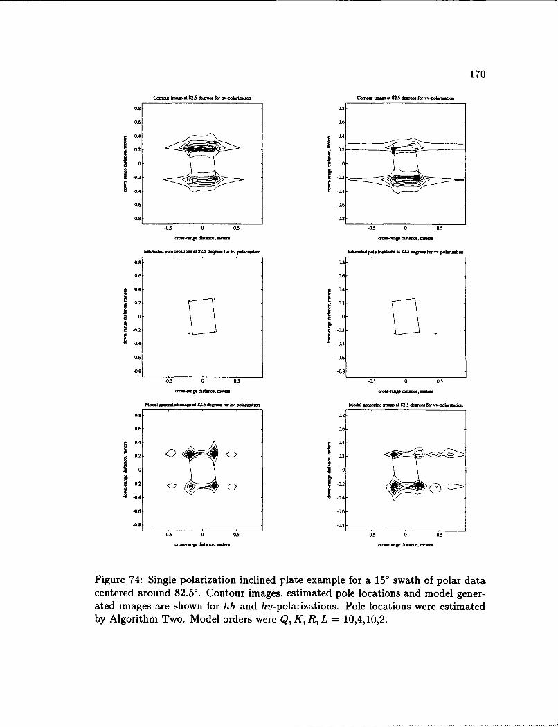
170
CUtotr imap t 82.5 deg for h-pdomaat Cioon iat 82.5 dwur for --polarmh
0.8- 0.9
0.6- 0.6-
I 0.4 __4
0.2
-0.6 -0.6
-0.8 -0.8
-0.5 0 0.5 -0.5 0 0.5
mv-atge datae, meten coum-ranp dkaomar
Eatuted pole locabti st 82.5 doegmc for hv-polaizatbon Esimated pole tombns at 82.5 dgm for w-polarnoatio
0.8- 0.8
0.6 0.6
0. - 0.4-
I 0.2 -0.2
.0 1.0.2-0.2
I.0.4 -E -O
-0.6 -0.6
-0.8 -0.8
0.5 0 0.5 -0.5 0 0.5
ora-ng ditaote, mce. arowgo dt.1U, meters
Model rlonrted uogr at 82.5 degrees for hv-polnawtio Model pcoerakd ansp at 82.5 dr= for -polan-o
0.8 0.:
0.6 0.6
OA 0.4-
0.2 >0.2
-0.2 K -0.2
0.4- -0.4-0.6 -0.6
-0.8 -0.
-0.5 0 0.5 -0.5 0 0.5
o ;oi-r o dtanoe, .bre csm-nog dutancn mew.s
Figure 74: Single polarization inclined rlate example for a 150 swath of polar datacentered around 82.50. Contour images, estimated pole locations and model gener-ated images are shown for hh and hv-polarizations. Pole locations were estimatedby Algorithm Two. Model orders were Q, K, R, L = 10,4,10,2.
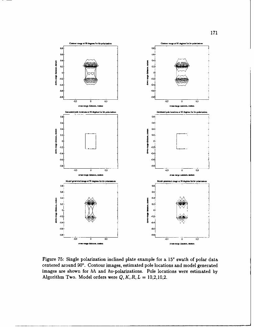
171
lmfifif -Va 90 &Wmg fm hamaknba Call...- .. p 190-kg~mfrw h,-podmb
0.8 as
0.6 0.6
0.4 0.4
0.2 02
0 0t-0. t-0.2-0.4 144-0.6 -0.6
-0.8 -0.8
-0.5 0 0.5 -0 0 0.5o-rnp dhLst, mak €lm w Mn
E.tuiatd pole IoC.t.s at 90 deg.... fa hh-pok rmbw Ehwakd pok l c.ab t 90 dWm. fmr hv-polruva
0.8 0.8
0.6 0.6
0.4- 0.4
0.2 01
10,10
-0.2 -0.2
-0.4 -0.4
-0.6 -0.6
-0.5 0 0,3 -0.5 0 0.5
-. rnp dvti..e, metar mel..e d-=e m,.In
Model gmr&mdage att 9 0
depF. for hh-polnzeon Model gammed map g0 deatr90 for bV-polmn..
0.8 0.8
0.6 0.6
0.4- 0.4- j
0.2 0.2
0 0
-0.2 -0.2
-0.4
-0.6 -0.6
-0.8 -0.9
-0.5 0 0.5 -0.5 0 0.5
¢ro-nmw dwtme ra Wr dro s.nu .d lafm
Figure 75: Single polarization inclined plate example for a 150 swath of polar datacentered around 900. Contour images, estimated pole locations and model generatedimages are shown for hh and hv-polarizations. Pole locations were estimated byAlgorithm Two. Model orders were Q, K, R, L = 10,2,10,2.
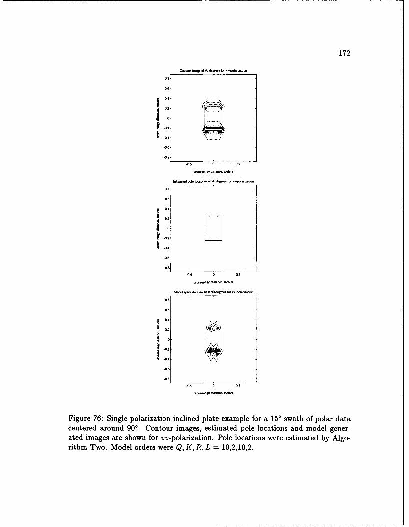
172
CQtow- @ 190 dcgr e -polanMo
0.8
0.6
0.2
10
-02-
1 -0.4
41.6
-0.8
-0.5 0 05
0.8
0.6-
0.4
jo4.2
1-0.4
-0.8
-0. 0 0.5
ad- m , mesers
Model gerted omp at 9
0 de ea for -polizm
0.8-
0.6
0.4
0.2
10
-0.2
-0.4
-06.
-03 0 0.5
Figure 76: Single polarization inclined plate example for a 150 swath of polar datacentered around 900. Contour images, estimated pole locations and model gener-ated images are shown for vv-polarization. Pole locations were estimated by Algo-rithm Two. Model orders were Q, K, R, L = 10,2,10,2.

173
(the edge at x=-0.173 meters, between C1 and C2, in Figure 59) is dominant in the
vv-polarization response. The estimated pole locations confirm this as they cluster
on the dominant edge in the hh and vv-polarization cases. For the hv-polarization
response, the corners C1 and C2 are dominant.
Figures 66 and 67 show results for 0 = 15'. From the contour images it can be
seen that this response is corner dominated. This can also be seen in the estimated
pole plots. The same conclusions can be made for the scenarios analyzed in Fig-
ures 68 through 73. Figures 73 and 74 show the results for 0 = 82.50. This is an
edge dominated scenario similar to the 0 = 7.5' scenario. For many of the scenarios,
some corners or edges are dominant for one polarization while the other edges or
corners are dominant for another polarization. This can be taken advantage of by
estimating the pole locations using the full-polarization data, and this is done in the
next section.
The estimated pole locations in Figures 63 through 76, in general, lie on the
corners of the plate. For many of the plots, one corner of the plate has several poles
clustering on it and other corner(s) of the plate have no poles associated with them.
In these cases, the corner with more than one associated pole is usually the largest
energy corner on the plate, which can be seen by looking at the image of the plate.
Also, the corner(s) with no associated poles is usually the lowest energy corner(s).
The model generated contour images should, ideally, be identical to the original
data plate images. However, there are differences between the two sets of images.
These differences demonstrate that the 2-D Prony Model has difficulty in modeling
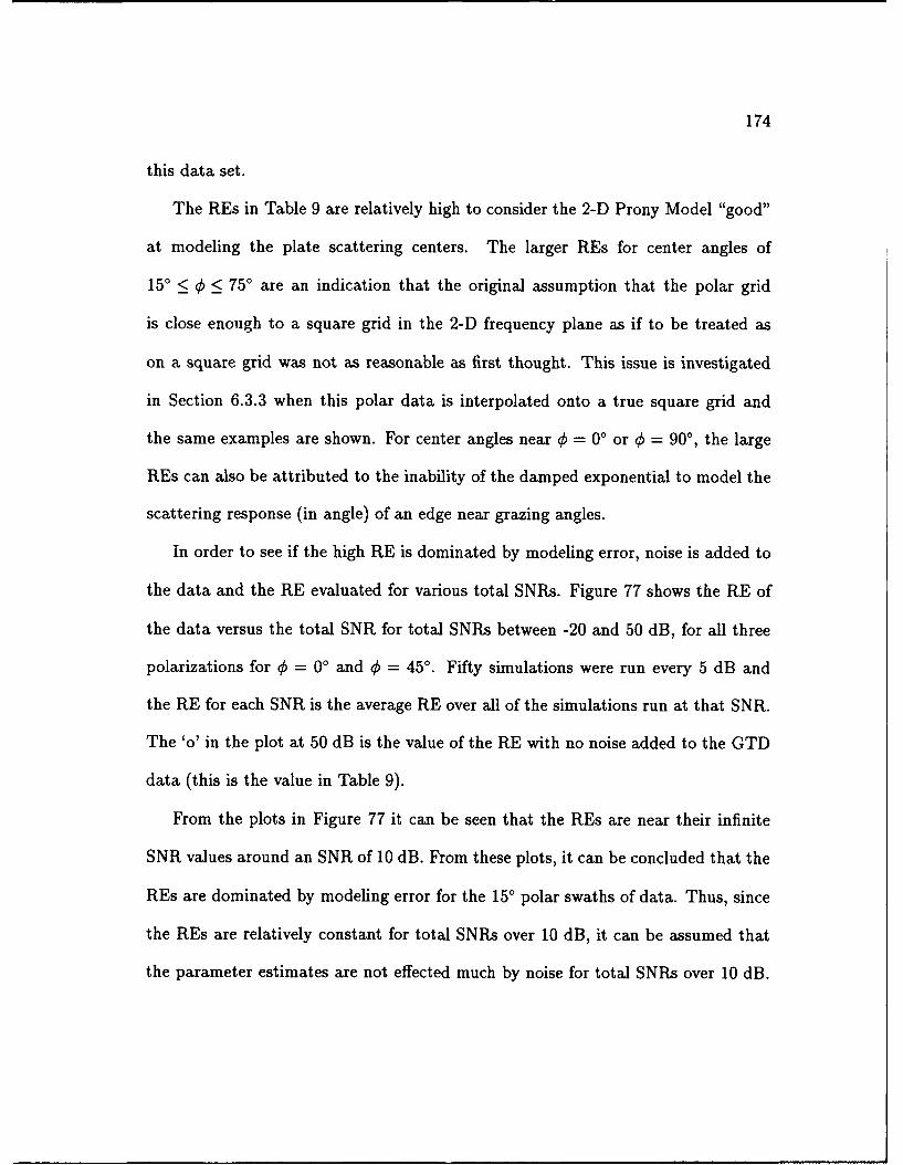
174
this data set.
The REs in Table 9 are relatively high to consider the 2-D Prony Model "good"
at modeling the plate scattering centers. The larger REs for center angles of
150 < 0 < 750 are an indication that the original assumption that the polar grid
is close enough to a square grid in the 2-D frequency plane as if to be treated as
on a square grid was not as reasonable as first thought. This issue is investigated
in Section 6.3.3 when this polar data is interpolated onto a true square grid and
the same examples are shown. For center angles near 0 = 0' or 4 = 90', the large
REs can also be attributed to the inability of the damped exponential to model the
scattering response (in angle) of an edge near grazing angles.
In order to see if the high RE is dominated by modeling error, noise is added to
the data and the RE evaluated for various total SNRs. Figure 77 shows the RE of
the data versus the total SNR for total SNRs between -20 and 50 dB, for all three
polarizations for 4, = 00 and 0 = 450 . Fifty simulations were run every 5 dB and
the RE for each SNR is the average RE over all of the simulations run at that SNR.
The 'o' in the plot at 50 dB is the value of the RE with no noise added to the GTD
data (this is the value in Table 9).
From the plots in Figure 77 it can be seen that the REs are near their infinite
SNR values around an SNR of 10 dB. From these plots, it can be concluded that the
REs are dominated by modeling error for the 15' polar swaths of data. Thus, since
the REs are relatively constant for total SNRs over 10 dB, it can be assumed that
the parameter estimates are not effected much by noise for total SNRs over 10 dB.
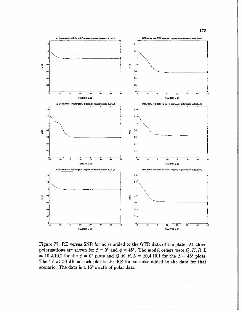
175MSE oalb SNR for ph,4) egm. Mrjpolnnbo ..r K.L=2.2 MSE s~.total SNE lot pborS dur=s. b-poorlanzat anrd LL-4,1
1.4- 1.4-
1.2 1.2
u1 0.8 OL
0L6 0.6
0.4 0.4
0.2 0.2
-20 -10 0 10 20 30 40 50 -20 -to 0 10 20 30 40 so
Totl SNR dB Total SNRin odB
MSE oal! SNR for ph.O &po., Jr-polamatmor and K.Lo2,2 MSE..rnu total SNR for pho=45 tdgoes, ha-pohnzabor and K.Lo4.l
1.4- 1.4-
1.2 1.2
to 0.8- OLS 8
0.6- 0.6-
0.4- 0.4
0.2- 0.2
-20 -10 0 t0 20 30 40 s0 -20 -10 0 10 20 30 40 s
Total SNE R dB Total SNR to dB
MSE toalo SNR for phu=O d.Vagrr 'v-polsrmtmo sAd K.L=2,2 MSE toalos SNE foc ph.=45 dg,- vv-polnorbo, and K.L.4,1
1.4[ 1.4-
1.2 1.2
0.6 069
0.4 0.4-
0.2- 0.2-
-20 -10 10 20 3 .0 40 30 0 0 - -1 0; 10 20 30 40 30
Totsl S nR tdB Tots! S" odB
Figure 77: RE versus SNR for noise added to the GTD data of the plate. All threepolarizations are shown for 4 = 00 and 0 = 450* The model orders were Q, K, R, L= 10,2,10,2 for the 0 = 00 plots and Q, K, R, L = 10,4,10,1 for the 0 = 450 plots.The 'o' at 50 dB in each plot is the RE for no noise added to the data for thatscenario. The data is a 150 swath of polar data.
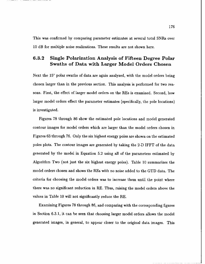
176
This was confirmed by comparing parameter estimates at several total SNRs over
10 dB for multiple noise realizations. These results are not shown here.
6.3.2 Single Polarization Analysis of Fifteen Degree PolarSwaths of Data with Larger Model Orders Chosen
Next the 150 polar swaths of data are again analyzed, with the model orders being
chosen larger than in the previous section. This analysis is performed for two rea-
sons. First, the effect of larger model orders on the REs is examined. Second, how
larger model orders effect the parameter estimates (specifically, the pole locations)
is investigated.
Figures 78 through 86 show the estimated pole locations and model generated
contour images for model orders which are larger than the model orders chosen in
Figures 63 through 76. Only the six highest energy poles are shown on the estimated
poles plots. The contour images are generated by taking the 2-D IFFT of the data
generated by the model in Equation 5.2 using all of the parameters estimated by
Algorithm Two (not just the six highest energy poles). Table 10 summarizes the
model orders chosen and shows the REs with no noise added to the GTD data. The
criteria for choosing the model orders was to increase them until the point where
there was no significant reduction in RE. Thus, raising the model orders above the
values in Table 10 will not significantly reduce the RE.
Examining Figures 78 through 86, and comparing with the corresponding figures
in Section 6.3.1, it can be seen that choosing larger model orders allows the model
generated images, in general, to appear closer to the original data images. This
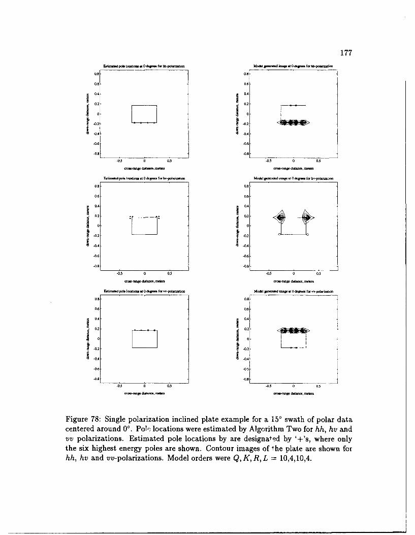
177
Fitimsted pole loacao at 0 dm.pea for hb-polstnuton Moda sweled Mae .t 0 dee. ft. bb-polrnltmn
0.8 0.8
06 0.6-
04 0.4
0.2 02
-. 2 -01
-0.4- -0.4-
4.6 -0.6
-0.8 -0.8
-0.5 0 0.5 -05 0 0.5
r-enoe dwlno., mdae o.-rege dula, meters
Estumaed pole locarto at 0 ognees for he-poltnzatio Model gemated mege at 0 depm for hv-polanruab
0.8 0.8
0.6 0.6
0.4 j 0.4
10 0.20 0-0.2 -01
-- 0.4
-0.6 -0.6
-0.8 4.9
-0.5 0 0.5 -0.5 0 0.5
crow-range diot&=c. eters oa-roge di..m
Easbaled pole locatora at 0 dleroat for w-poluization Model generaled dume at 0 deme for w-polaenoon
0.8 0.8
0.6 0.6
0.4- 0.4
, 4.2 = 0.210 10
-02 -0.2
-0.6 -046
-0.8 -0.8
-0-5 0 0.5 0. 5 0 05
orr.-rmnge did-ne, crow-range daam .Ws,
Figure 78: Single polarization inclined plate example for a 150 swath of polar datacentered around 0'. Pohc locations were estimated by Algorithm Two for hh, hv andvv polarizations. Estimated pole locations by are designated by '+'s, where onlythe six highest energy poles are shown. Contour images of the plate are shown forhh, hv and vv-polarizations. Model orders were Q, K, R, L = 10,4,10,4.
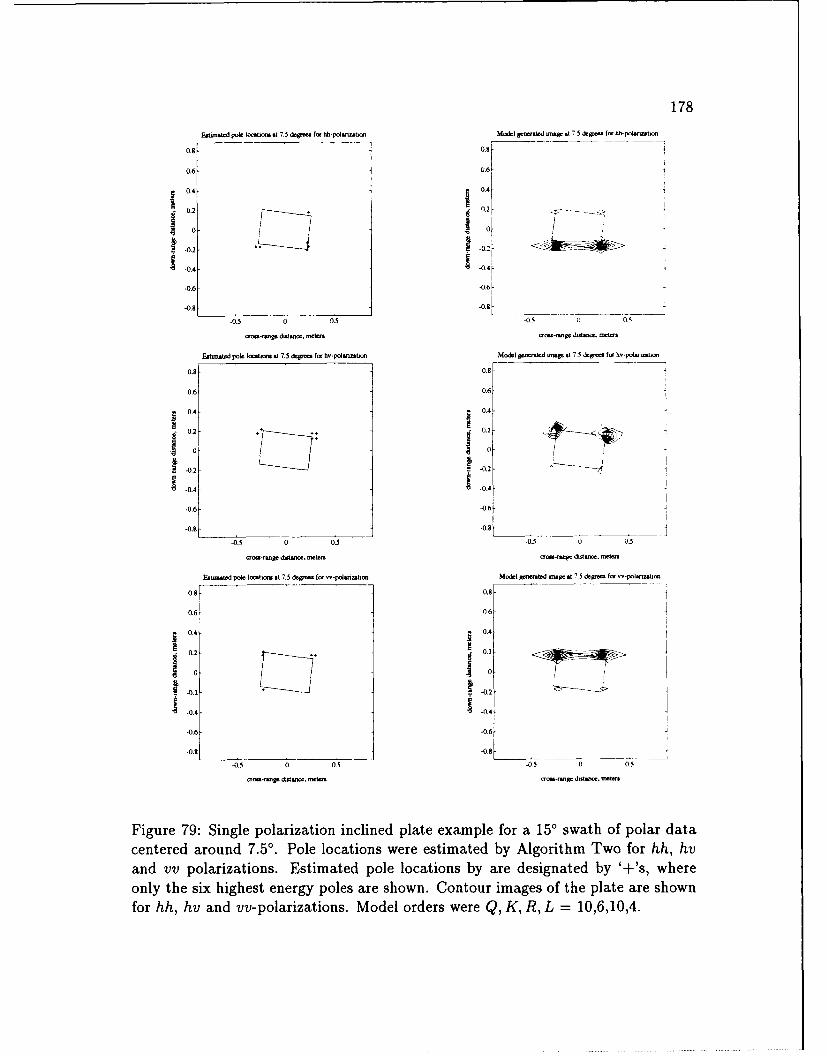
178
Edmitod po Ioi_ .t 7.5 &- f. hh-polma= Mo.I gm. d .W .17 5 - g- f- hh-p.L.tt
0.8 0.84
0.6 U.6
0.4 0.4
0.2 0 02
0 0
-0.4 -0.4 .
-0.6 -40 .
-0.8
-0.5 0 0.5 -0.5 0.5
.mo-rwpg dw ,c., mt-r _t - 9.g diltivmtr
Estmod po k . 7.5 dg- for h-polzmtlO Mod, Wfed W s 7.5 g s fr hv-pol-W--tot-
0.8- 0.81 1
0.6- 0.6
0.4- 0.41-
N 0
-0- -0.2
-0.4 -0.4-
-0..6--0 . 6- -0.84
-0.5 0 0.5 -0.5 0 0.5
EUmt.td pole loctios at 7.5 deg.. fo w-polmmhz Modol g td mac t 75 dowo'. f. vo-pol.r.UI o.
0.8 0.8
0.6 06 -
- 0.4-- 0.4-1
N 0.2 0.
0 0-0.2- -0.2 ~'
1 -0.4- 0.
-0.6 -0.61
-0.8 -0.8
-0.5 0 0.5 -0.5 0 03
a -g dirt 1, .tml-mg ltn -rm
Figure 79: Single polarization inclined plate example for a 150 swath of polar datacentered around 7.5' . Pole locations were estimated by Algorithm Two for hh, hvand vv polarizations. Estimated pole locations by are designated by '+'s, whereonly the six highest energy poles are shown. Contour images of the plate are shownfor hh, hv and vv-polarizations. Model orders were Q, K, R, L = 10,6,10,4.
179
EUit.1ed pot. Ioo- t 15 dqp- f. hh-lonzmo- Mod g.td .W a15 &grv. for hh-pohtW.St
0.6 0.6
0.4 0.4
0.2 02
0 0.
-0.2 - -0.
-0.6 -046
-0.8 -0.8
-0.5 0 0.5 -0.5 0 0.5
.rmo-..ge dwt, 0101o10..r0 d*o oea m
Famated p!de locabuos 15 t gSeg for hv-potanntiu Model em-rald m It 15 dc gr fmr bv-oW=lUrl
0.8 0.8
0.6 0.6
0.4- 0.4
02 0.20 .2
-0.2 -02
-0.4 1 -0.4
-0.6 -0.6
-0.8 -0.8
-0.5 0 0.5 - .4- 0 0
aru,-ne d..tsor, metOOs I48 drou-sn or orme
Esormt-d pole Iocobm st 15 deg-e f. v-polariobmo Model gwwwd uno. .115 I for e-polw.=Wm
0.8 0.8
0.6 0.6
0.4-j 0.4-
0.2 0.2
10 10
-0.2 -0.2
-0.4 .0.4
-0.6 -0.6
-0.8 .8L
-0.0 0 0.5 -0.5 0 0.5
ora-.nge dialn, metws oro-rne8. duon., rnet.
Figure 80: Single polarization inclined plate example for a 150 swath of polar datacentered around 150. Pole locations were estimated by Algorithm Two for hh, hvand vv polarizations. Estimated pole locations by are designated by '+'s, whereonly the six highest energy poles are shown. Contour images of the plate are shownfor hh, hv and vv-polarizations. Model orders were Q, K, R, L = 10,6,10,4.
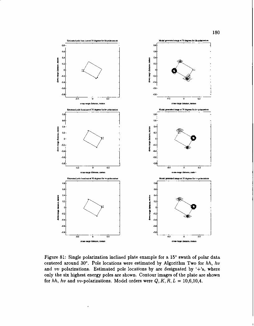
180
E.tmeOMd pole l-tio w 30 dog- fo hh-polWbtacn Model 8k mae at 30 d for hbixdIarmbn
0.8 0.
0.6 0.6
I 0.4- 0.4
g0.2-0
-.0.4 -0.4-0.6 -0.6
-0.8 .0.8
-0.5 0 0.5 05 0 0.5
.=-=go dwatnc mele, €new- n g diame, met
Est uemid pole Iocaions at 30 degien few hv-polanz tiut Mol g m t 30 dege as for hv-oltibm
0.8 0.8
0.6 0.6
0.2 0.2
0~ 0
I-0.2 0.2/.0.4 1..-0.6 -064-0.6 -0.6
-0.5 0 0.5 -0-5 0 0.5
crms-rnge dustanct. ror. a dift.r .e, de-
Eitmated pole lcaons at 30 dgreeg for w-pohnzmaon Model gmemkd -F at 30 dm for wpoorodian
0.8 0.8
0.6 0.6-
0.4- 0.4.
0.2 0.2
00
I -0.2 -0.2
.0.4 -0.4
-0.6 -0.6
-0.8 -0.8
-0.5 0 0.5 -0.5 0 0.5
crmu-@eg diauuo, metor, dewe dontnt
Figure 81: Single polarization inclined plate example for a 150 swath of polar datacentered around 300. Pole locations were estimated by Algorithm Two for hh, hvand vv polarizations. Estimated pole locations by are designated by '+'s, whereonly the six highest energy poles are shown. Contour images of the plate are shownfor hh, hv and vv-polarizations. Model orders were Q, K, R, L = 10,6,10,4.
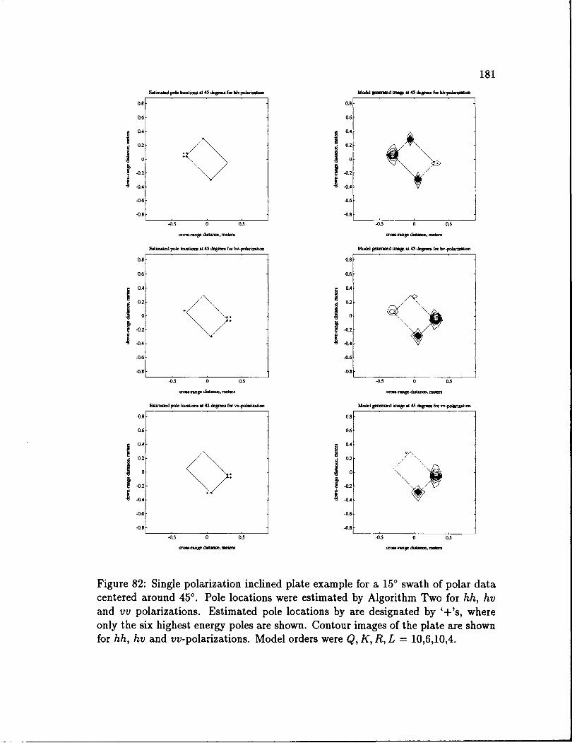
181Ed.1.d pdlo cawm at 45 depte. fm hh-pohsnl 84o& V.W up at45 &V- far W.-p.Wx~ab
0.6 0.6
064 064
0.2 042
00
.0.2 .2
-064 -064
-0.8 -0.8
-08 -0.,5 0 0.50. -05 0 0.5
EateId pole loesi at 45 degroo foa hv-polarizhoe ModrI gmenlod mnp at145 depocs fmr hv-anzabwo
0.8- 0.8
0.6- 0.6-
0.4 0.4-
0.2 0.2
10 1012 -0.2
0.4- -0.4-0.6- -0.6
-0.98 -08
-0.5 0 0.5 -0.5 0 0.5
cross-Vg d~sts-c mews11 cmasrange di.1.ror amer
E.Utods pole loeslm. at45 degiaoo fom -polsrioetio ho&I pmrsted iraW at4 5
dpmr for oo-polrnzafl
0.8- 0.8-
0.6- 0.6-
i 0.4- 0.4-
0.2 01210 10- /
I -0.2 -0.2-
-0.4 -0.4-
-0.6 -0.6
-0.5 0 0.5 -0.5 0 0.5
ormlg. dd-o, mews1r -- Vp dWW10e. W.b
Figure 82: Single polarization inclined plate example for a 150 swath of polar datacentered around 450. Pole locations were estimated by Algorithm Two for hh, hvand vv polarizations. Estimated pole locations by are designated by '+'s, whereonly the six highest energy poles are shown. Contour images of the plate are shownfor hh, hv and vv-polarizations. Model orders were Q, K, R, L = 10,6,10,4.
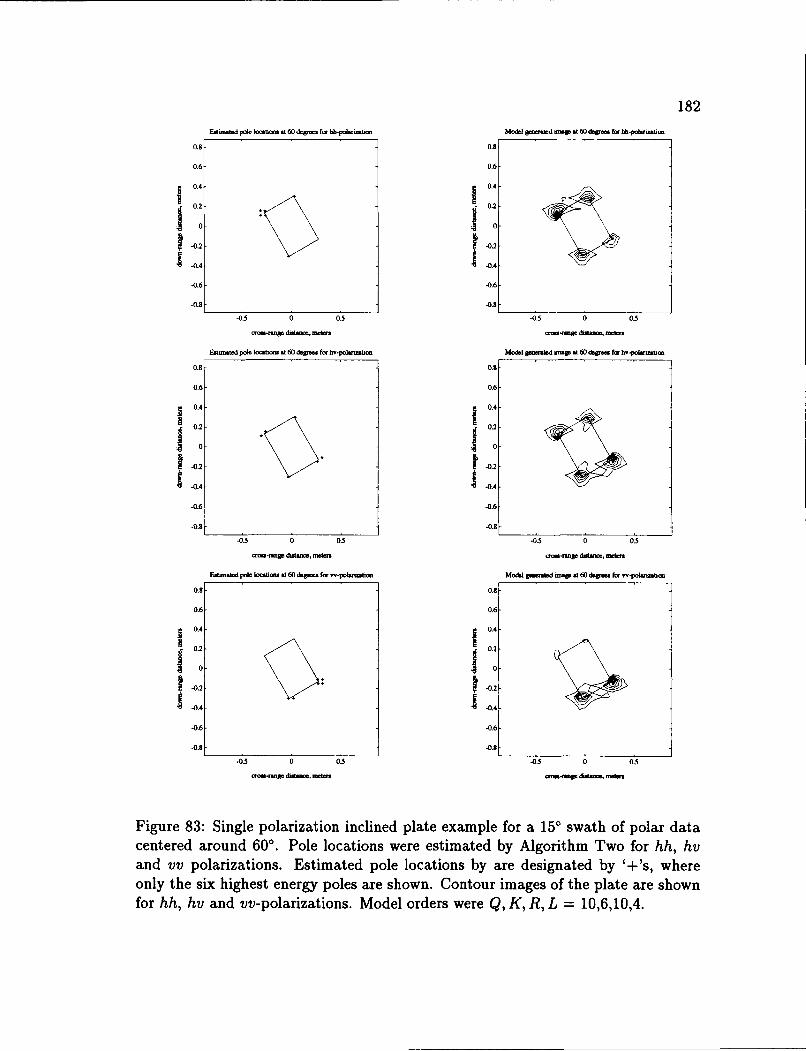
182Edii.i..do lopdcbm at 60 &g- fdr hhp.- M.od @p=,d ump d 60 d&. f6. bh-poi.rmha.
0.8 0.8
0.6 0.6
I0.4- 04-
-0.2 -0.2
-0.6- -0.6
-0.8 -0.8
-0.5 0 0.5 -0.5 0 0.5cro -rg dijoaoc., mer. cou.mp dismm. nets
EAitted pole locatboc at 60 dcgte.. for hv.poltonrittm Model gailtd rma at 60 degees fbr hv-polnmm
0.8 0.8
0.6- 0.6
0.4- 0.4-
0.2 02
0 0
1 -0.2-0.4- -0.4
-0.6- -0.6
-0.8 -0.8
-0.5 0 0.5 -0.5 0 0.5
ori..nge dtam., me a-nmp dotum, ma
Eumated po lotctm at 60 degma fm w-polrusttan Model gmratd mmp at 60 da. for -poWtmu
0.8 0.8
0.6- 0.6
0 0.4- 0.4
10.22
-0.4- -0.44.6 -0.6
-0.8 -0.8
-0.5 0 05 -05 0 0.5
mr tg-a diatm, mam6r orw-na diaim, mtm
Figure 83: Single polarization inclined plate example for a 150 swath of polar datacentered around 600. Pole locations were estimated by Algorithm Two for hh, hvand vv polarizations. Estimated pole locations by are designated by '+'s, whereonly the six highest energy poles are shown. Contour images of the plate are shownfor hh, hv and vv-polarizations. Model orders were Q, K, R, L = 10,6,10,4.
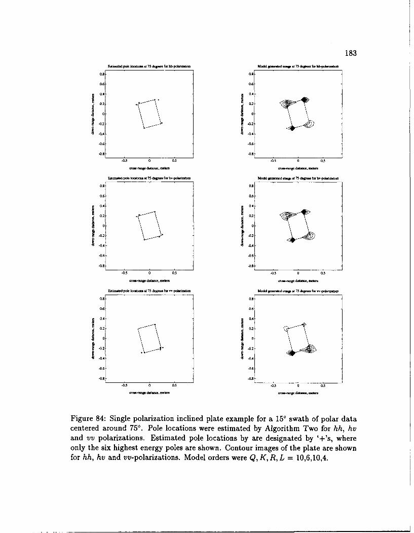
183
Ed=&tsd pole loomebat 75 dW fo, hh-pol~musa Modl Semed a .75 &Urin fo, hb -puolo
0.8 0.8
0.6 0.6
0.4 0.4
0 100. 2 i--0.2 -0.2
-0.6- -0.6
-0.8 -0.2
-0.5 0 0.5 -05 0 0.5
-reage distane, mobf mweu d-in-, mkn1
Eatboted pole bcoatico .75 d ge hr.pono~lcm Mode.-.Id amp A 75 degree Fr hv-polrmo
0.8 0.8
0.6 0.6
0.4- 0.4-
0.2 8 0.2
-0I -0.204- 0.4
-0.6 -0.6
-0.g -.0.8 _____________________1
-0.5 0 0.5 -0.5 0 0.5
aom.'age distance, oe. a-W dcea ete lm
E.tunated po e locatios at 75 dIes for w-polarizatio Model @em.ted uap i 75 degrees l e--poheebw
0.8 0.8
0.6 0,6
0.4- 0.4-
0,2 0.2
0 0I -0.2 I -0.2
-0.4 1.0.4-0.6 -0.6
-0.8 -0.8
-0.5 0 0.5 -0. 0 0.5
C-r-gle dolte. dut. .ro-lge dhsen .
Figure 84: Single polarization inclined plate example for a 150 swath of polar datacentered around 75' . Pole locations were estimated by Algorithm Two for hh, hvand vv polarizations. Estimated pole locations by are designated by '+'s, whereonly the six highest energy poles are shown. Contour images of the plate are shownfor hh, hv and vv-polarizations. Model orders were Q, K, R, L = 10,6,10,4.
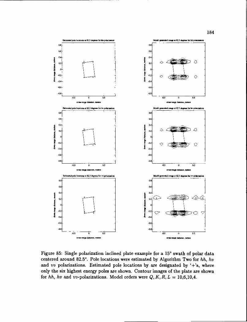
184
Eattmd pow. locato st 8235 degm fa to. hotnuwto Mo&I e6 at-d mw at 82.5 dw-t fm. 66-polanztt
0.8- 01
0.6- 0.6-
0.4 0.4-
0.2 1
00
-0.2 12 <
-0.6- 06
-0.8- -0,8
-0.5 0 0.5 -0.5 0 0.5
o~-~pdt mt..mt. o o- t8 dtflnom mom.
F..ttated polochtat at 82.5 ftgom to.topokrutm ~ MoI goctmted .aap at 82.5 dcg f. h-potartatto
0.8- 0.8-
0.6- 0.6-
0.4- 0.4
0.2 1
10S-0.2
021
I -0.4 -0.4
-0.6 -0.6-
-0.8 -0.98
-0.5 0 0.5 -0.5 0 0.5
Esttmab~d pole locatico at 82.5 dest.. to. opo~attzaso MoMe genwkd wmw8 at 82.5 dwmoe fa. wowlrmhc
0.8 0.8-
0.6- 0.6-
0.4 - 0.4-
0.2 .
. 0 10
-0.2 1-0.2
1.0.4 -.
-0.6 -0.6
-0.8 ________________________. -0.8-0.5 0 05 -05 0 053
Figure 85: Single polarization inclined plate example for a 15' swath of polar datacentered around 82.50. Pole locations were estimated by Algorithm Two for hh, hvand vv polarizations. Estimated pole locations by are designated by '+'s, whereonly the six highest energy poles are shown. Contour images of the plate are shownfor hh, hv and vv- polarizations. Model orders were Q, K, R, L = 10,6,10,4.
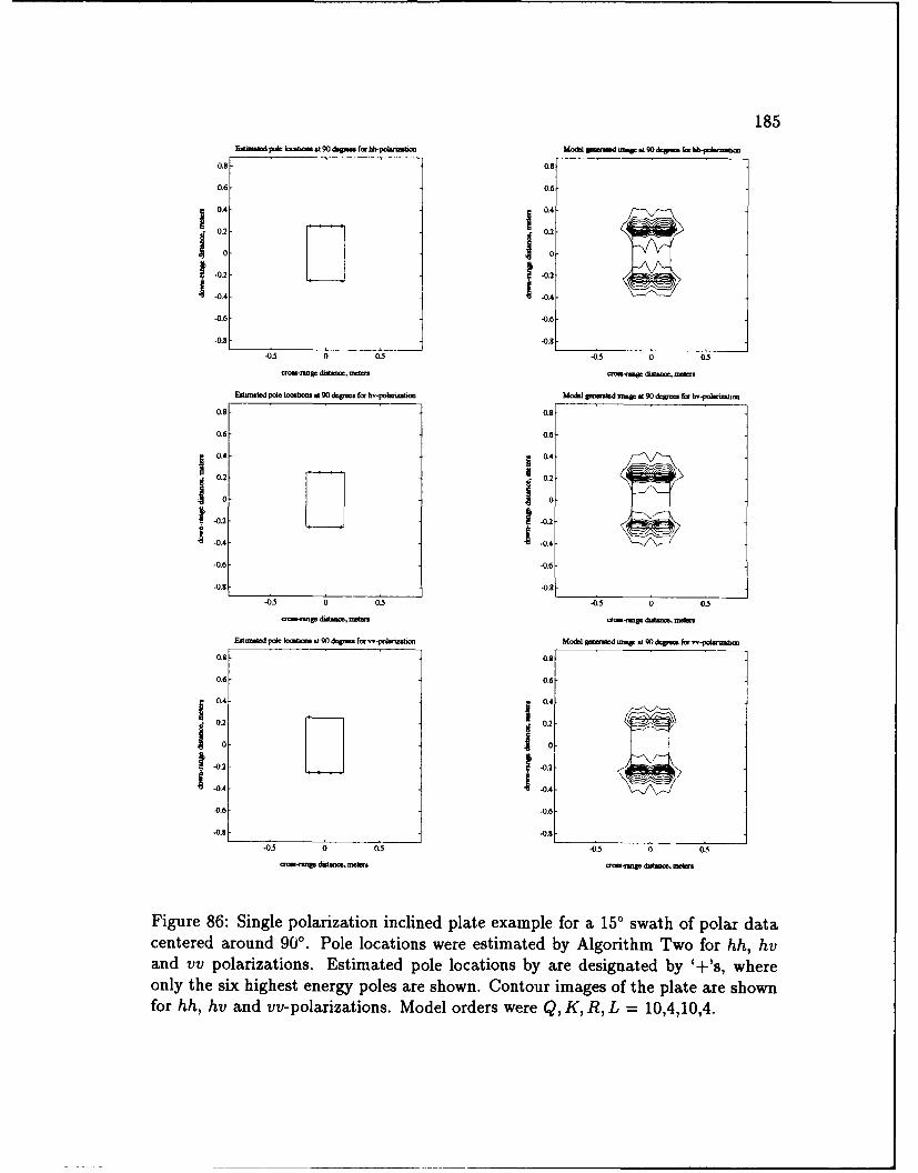
185Eatmid poic b.s a 90 dap f d hb-pomnatw Mom emembd akW a gO9&V fr. bh-pohm
0.8 0.8
0.6 0.6
0.4- 0.4-
0.2- 0.2
0--0.2-. -0.2.0.4 -0.4
-0.6 -0.
-0.8 -0.8
-0.5 0 0.5 -0.5 0 0.5
a-fnge diwtenor, mtw r di.-n r -A
Etmanbd pde locao at 90 degree fr hv-polknboat Mod eS pzatd onap at 90 ftr for hv-on.=bm
0.8 0.8
0.6 0.6
0.4- 04
0.2 - 0.2
-0.2 -0.2
-0.8 1 -0.8
-0.6 -0.6
-0.8 -0.6
-0.5 0 0.5 0.5 0 0.5
organe dLOA, me tre or-t dm, Omt
Estmaed pole lomabru at 90 dee fo w-ponzat Model guard t a 0 de90ee for r,-pobvmmh
0.8 0.8-
0.6 0.6-
0.4- 0.4-
0.2 10.2 ~
t -0.2 -0.2
-04 -0.41
-0.6 -0.6
-0.8- -0.8-0.5 0 0.5 -0.5 0 0.5
dwreea dawta .esooomedatmtr- e
Figure 86: Single polarization inclined plate example for a 15' swath of polar datacentered around 900. Pole locations were estimated by Algorithm Two for hh, hvand vv polarizations. Estimated pole locations by are designated by '+'s, whereonly the six highest energy poles are shown. Contour images of the plate are shownfor hh, hv and vv-polarizations. Model orders were Q, K, R, L = 10,4,10,4.
186
is reflected by the REs in Table 10 which are lower than their respective REs in
Table 9. The pole locations in Figures 78 through 86 tend to cluster multiple poles
on the largest energy corners or edges. Thus, the larger energy scattering centers
on the plate are modeled by several poles, and this reduces the REs.
The use of model orders which are larger than the expected number of scattering
centers is deviating from the intent of the 2-D TLS-Prony Technique to model one
scattering center by one 2-D mode. Ideally, the choice of model orders should reflect
the expected number of scattering centers. However, in cases where the damped
exponential does not model the scattering behavior of the scattering centers present
in the data, raising the model order will enable the 2-D damped exponential to
better model the data.
For this data set (the 150 polar swath of data) there are two reasons why the
2-D damped exponential model does not model the data well. First, for angles near
0 = 0 ' and 4 = 90', the response is edge dominated and the angular response
for these angles is impulsive which is not well modeled by a damped exponential.
Second, the initial assumption that the polar data can be used directly by the 2-D
TLS-Prony Technique was not as good as first assumed. This is demonstrated in the
next section (Section 6.3.3) when this polar data set is interpolated onto a square
grid.
Figure 87 shows the RE of the data versus the total SNR for total SNRs between
-20 and 50 dB, for all three polarizations for 0 = 00 and 0 = 45' . As before, fifty
simulations were run every 5 dB and the RE for each SNR is the average RE over all
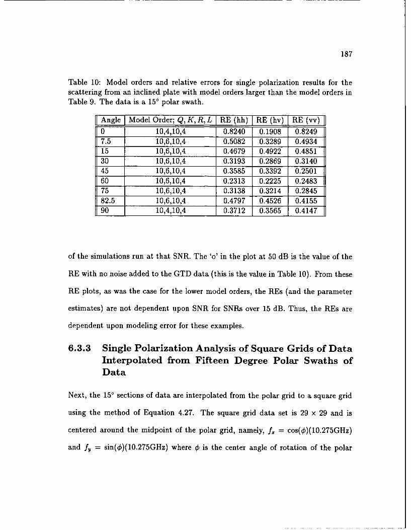
187
Table 10: Model orders and relative errors for single polarization results for thescattering from an inclined plate with model orders larger than the model orders inTable 9. The data is a 150 polar swath.
Angle J Model Order; Q, K, R, L RE (hh) RE (hv) RE (vv)0 10,4,10,4 0.8240 0.1908 0.82497.5 10,6,10,4 0.5082 0.3289 0.493415 10,6,10,4 0.4679 0.4922 0.485130 10,6,10,4 0.3193 0.2869 0.314045 10,6,10,4 0.3585 0.3392 0.250160 10,6,10,4 0.2313 0.2225 0.248375 10,6,10,4 0.3138 0.3214 0.284582.5 10,6,10,4 0.4797 0.4526 0.415590 10,4,10,4 0.3712 0.3565 0.4147
of the simulations run at that SNR. The 'o' in the plot at 50 dB is the value of the
RE with no noise added to the GTD data (this is the value in Table 10). From these
RE plots, as was the case for the lower model orders, the REs (and the parameter
estimates) are not dependent upon SNR for SNRs over 15 dB. Thus, the REs are
dependent upon modeling error for these examples.
6.3.3 Single Polarization Analysis of Square Grids of DataInterpolated from Fifteen Degree Polar Swaths ofData
Next, the 15' sections of data are interpolated from the polar grid to a square grid
using the method of Equation 4.27. The square grid data set is 29 x 29 and is
centered around the midpoint of the polar grid, namely, f2, = cos(¢)(10.275GHz)
and fy = sin(¢)(10.275GHz) where € is the center angle of rotation of the polar
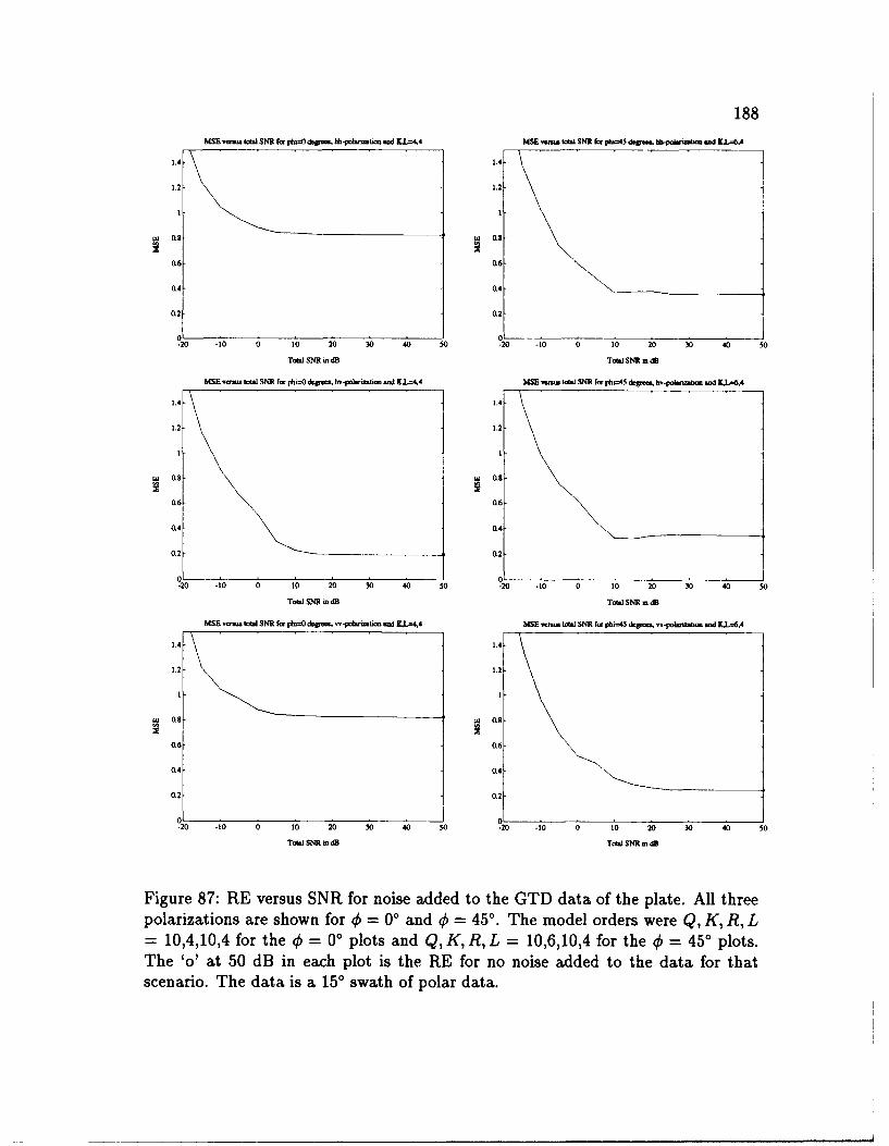
188MSE -auti total SNR fin p4i=&go . khi-,Wl. aW K.L-,C4 )4SE ne.tota SNR lor 0lo43 der... Wbpolertastm and K.L=6.
1.4 1.4
1.2 -1.2
0.6 0.6
0.4 0.4
0.2 0.2
01 _ _ __ _ _ __-20 -10 0 10 20 30 40 s0 -20 -10 0 10 20 30 40 s
Total SNR in dB Total SNR to 43l
MSE vini total Sf43 for p0&Odgrea, Iw-Polrnnboo and K.L=44 843 matte total Sf43 for ph454 dgmim, hn-polatim and L.L=64A
1.4 11.41.2- 1.2
1 1
Ow W. 4 0.
0.6 0.6
0.4- (.4
0.2- 0.2
01 01-20 -10 0 10 20 30 40 30 -20 -10 0 10 20 30 40 50
Total Sf43 m dB Total Sf43 to dB
MSE veria, total Sf43 for jptooO ,keoan vv-pola izalon &Wn K.L-4,4 MSE wn.total SNR for pitu=
4 dcrioaa n-poleneott and LLO-6.4
1.4-.4
1.
0.8 to 0.8
0.6 0.6
0.4 0.4
0.2 0.2
01 01-20 -10 0 t0 20 30 40 so -20 -10 0 10 20 30 40 s
Total SM4 to dB Total SM4 to dB
Figure 87: RE versus SNR for noise added to the GTD data of the plate. All threepolarizations are shown for 0 = 00 and 0 = 450. The model orders were Q, K, R, L= 10,4,10,4 for the 0 = 0* plots and Q, K, R, L = 10,6,10,4 for the 0 = 45' plots.The 'o' at 50 dB in each plot is the RE for no noise added to the data for thatscenario. The data is a 150 swath of polar data.
189
data. The steps in the square grid, in each direction, are 0.085 GHz. The square
grid is tilted on the 2-D frequency plane, by €, to account for the center angle of
rotation (0) of the data set. The local 2-D coordinate system for the square grid
data set is designated by rectilinear coordinates (ft, f 1) and these are related to
the absolute coordinates of the 2-D frequency plane, (f,, fy), which are shown in
Figure 61, by
f. = fx cos€- fy sine + fmid cos€ (6.2)
Y' = f, sin ¢ + A, cos € + fmid sin €
where fmid is the center frequency of the data set, which is 10.275 GHz for this
data set and € is the center angle rotation of the polar (and square) grid data sets.
Thus the square grid data set lies centered on this local coordinate system which is
translated and rotated from the absolute coordinates of the 2-D frequency plane.
The square grid was chosen to be slightly smaller than the polar grid from which
it was interpolated so that all of the data points on the square grid lie within the
boundaries of the original polar grid. This avoids the requirement to extrapolate for
data points on the square grid that would lie outside of the original polar grid. The
slightly reduced size of the square grid should have little effects on the resolution
capabilities of the 2-D TLS-Prony Technique. As before, the unambiguous range
for this scenario is 1.7637 meters in each direction, and this entire range is shown
in the figures which follow.
Figures 88 through 101 show the results for the square grid data. As for the
polar data based plots, shown for each center angle are three contour images of the
190
plate, each image corresponding to one of the three polarizations, found by directly
using the square grid data in the 2-D IFFT. Also shown are three sets of estimated
pole locations, each set corresponding to one of the three polarizations, estimated
by Algorithm Two with no noise added to the original data. In the cases where
there are more than four estimated poles, only the four highest energy poles are
shown in these plots. Along with these plots contour images are shown which were
generated from all of the estimated parameters (not just the four highest energy
poles). For each plot, the entire unambiguous range is shown. As stated before, all
of the contour images shown, in general, are on different magnitude scales. The REs
for the square grid examples are given in Table 11.
Since the square grid data is in the form required by the 2-D TLS-Prony Tech-
nique, the model orders are chosen to reflect the expected number of scattering
centers for the corner dominated scenarios, and slightly larger model orders are
used for edge dominated scenarios. Thus, for the corner dominated scenarios,
model orders of Q, K, R, L = 10, 4, 10, 1 are used; and for edge dominated scenarios,
Q, K, R, L = 10, 4,10, 2 and Q, K, R, L = 10, 2,10,2 are used.
Figures 88 through 101 show the results for the square grid data. Comparing
these results with the results for the 150 polar grid data, the original data images
for the square grid data are of slightly different form than the corresponding images
for the 15' polar grid data. The images for the square grid data are considered more
representative since the 2-D IFFT requires data on a square grid, not a polar grid.
Also, the estimated pole locations are, in general, closer to the corners of the plate
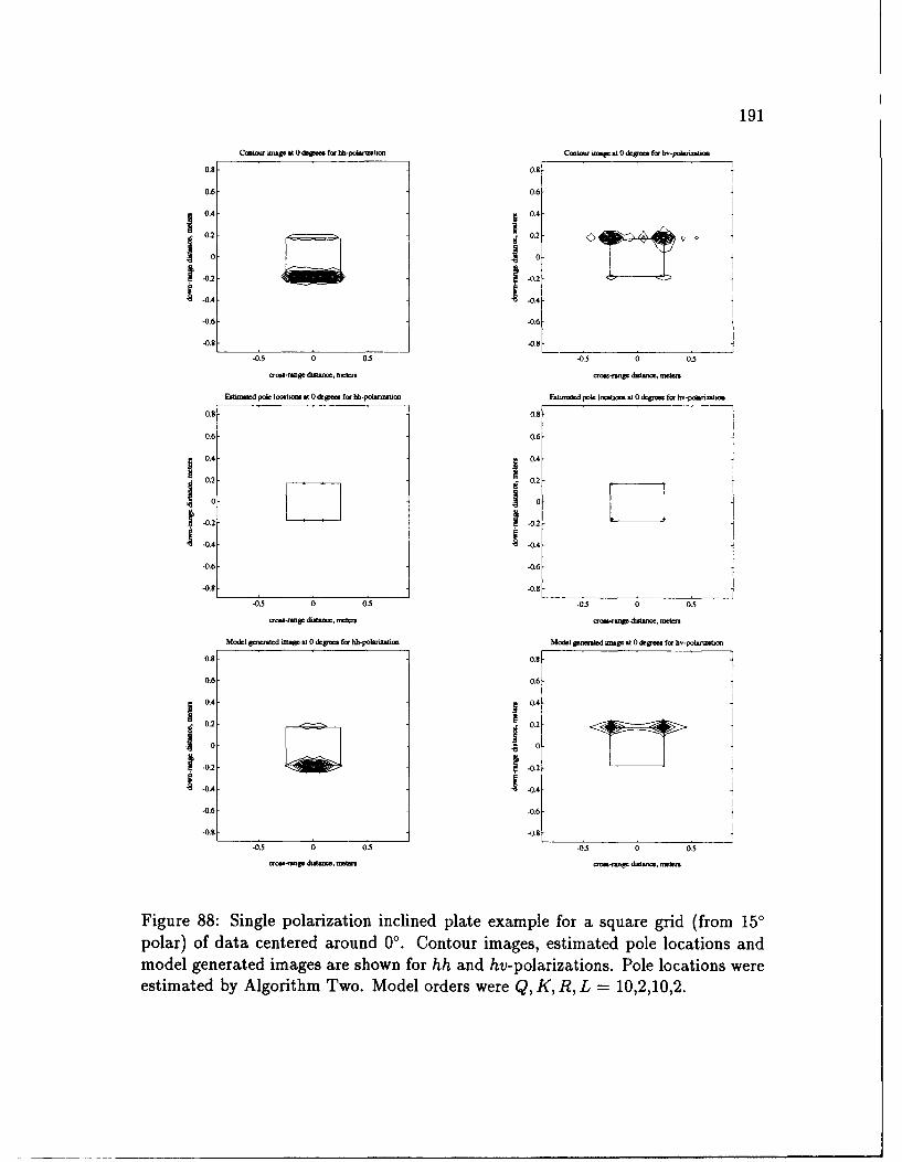
191
Camrao muW at 0 dca for hh-pokwlrm Cotow map at 0 dpme. for h-po no.t.o
0.8 0.8
0.6 06
0.4 6 0.4
-0.2 . 0.2-
I-0.4 14
-0.6- -0.6-
-08 4.8
-0.5 0 0.5 -05 0 0.5
a-o-g. dtamae, n o.-nge d-, metem
p.tansdol Iotpl.to at 0 degrees ft hh-poluization EatmaFed pole Iocions at 0 depm fo hv-pdwumb
0.8 0.8
0.6 0.6
0.4- 0.4
0- 0-0.2- -0.2
S-024 4
-0. -0.6
-0.9 -0.8
-0.5 0 0.5 -0.5 0 05
ow.-range ds ntwo, mel or.g-ne dua mo., mea
Model g.e...ltd map at0 d0 Vs for hh-polhrzabm Model gemntd mup at 0 degm for hv-polm usba
0.8 0.8-
0.6 0.6-
0 0
-0.2 -0.2
-0.6 -0.6-
-0.9 -0.8
-0.5 0 05 -0-5 0 0.5
o Vo-ng. diu..e, rnefam € -n.J, dflnmo, 0..
Figure 88: Single polarization inclined plate example for a square grid (from 150polar) of data centered around 00. Contour images, estimated pole locations andmodel generated images are shown for hh and hv-polarizations. Pole locations wereestimated by Algorithm Two. Model orders were Q, K, R, L = 10,2,10,2.
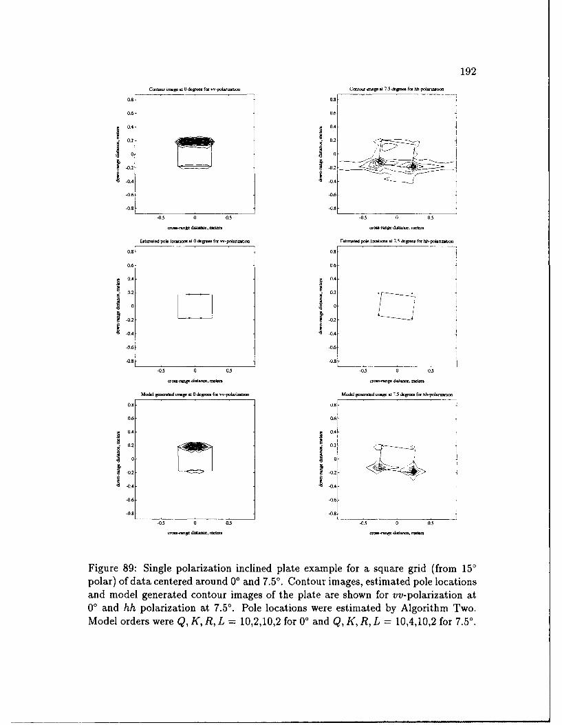
192Contour -Ws at 0 defee for vv-polwzt~m Contou -w .t7.5 dep f-r hb-pol-.Uo
0.8 o.s
0.6 0.6 t
0.4- 0.4-
0.2 -_ _ _ _ 0.2
00j j o0 0
S -0.2 -0.2
-0.4 -0.4
-0.6 -0.6 I
0.,8 -0.8-
-0.5 0 0.5 -0.5 0 05
c -ge disa-e, meten rc a dW-, a .W,
a.tlmatd pot. nto. t 0 cgvas for -- pln-.o F.s1ned pole Io. at 7.5 ,.p. ror hh-p0Im-bon
0.8 0.8
0.6 0.6
0.4- 0.4
0.2 0.2-U
1 F. 0 10/
0.2 -0.2
.0.4 -0.4-
06 -0.6
08 -0.8
-0.5 0 0.5 -0.5 0 0.5
Model g . mrad magt at 0 dcea for -polariton Model pml.dft unm. at 7.5 degree for hh-potanm.1.n
0.8 0.8-
0.6- 0.6-
0.4 0.4-
-0.2 -- 0.2-
-- 0.4- -0.4-
-0.6- -0.6-
-0.8 -0.8
-0.5 0 0.5 -0.5 0 0.5.r--g. dwatce, MO arm-g. d"rn, matw
Figure 89: Single polarization inclined plate example for a square grid (from 150polar) of data centered around 0' and 7.5' . Contour images, estimated pole locationsand model generated contour images of the plate are shown for vv-polarization at0' and hh polarization at 7.50 . Pole locations were estimated by Algorithm Two.Model orders were Q, K, R, L = 10,2,10,2 for 0' and Q, K, R, L = 10,4,10,2 for 7.50.
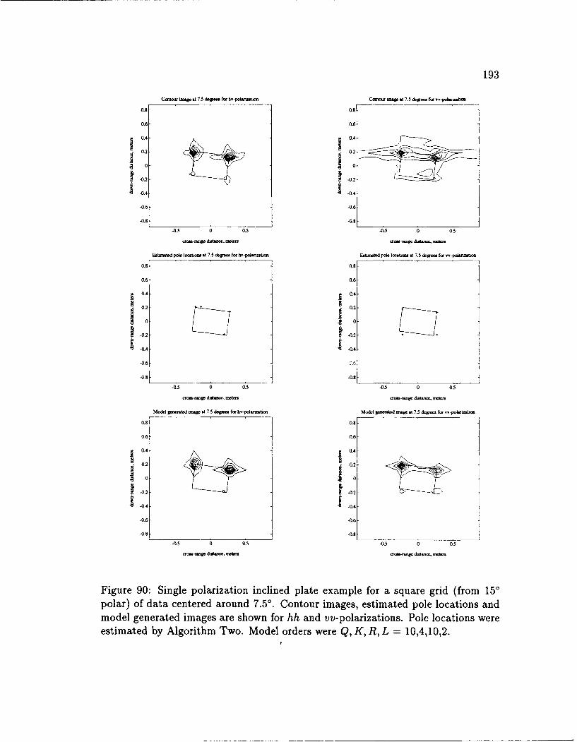
193
Cooto-r Imag 7.5 depg for ho-po mu Contour .ngW 7.5 degeee for -- pdole-nbe
0.8- 08.9
0.6 0.6
0.4- 0.4-0.o2- 0.2
-0.4 -0.4
-0.6 -0.6
-0.8 -0.
-0.5 0 0.5 -0.5 0 0.5
c-g.ge dioto€t, metesn eo-n d , metr
Eatmted pole locatin s 7.5 de.ge for hv-poltmontm EAtbed pole Io..t-a t 7.5 dege for -- potWnotm n
0.8 0.8
0.6 0.6
0.4-04
0.2 - 0.2
0 0
-0.2 -02
-0.4 1 -0.4
-0.6 2.t"
-. 8 -0.8t
-0.5 0 0.5 -0.5 0 05
cron-ege d ne.trs tot-nege d."r. mer
Model genamed mage A 7.5 degree for bv-polarzmton Model eted nage at 7.5 dgt'e foe vv-polaroater
0.8 0.8-
0,6- 0.6
0O.4
- .4-
0.2 0.2
10 10
.02-0.2 t 7!I-0.4- -0.4-
-0.6 -0.6
-0.8 -0.8
-0.5 0 0.5 -0.5 0 0.5
r -rage dtanoe, er r-gda ftem
Figure 90: Single polarization inclined plate example for a square grid (from 150polar) of data centered around 7.5'. Contour images, estimated pole locations andmodel generated images are shown for hh and vv-polarizations. Pole locations wereestimated by Algorithm Two. Model orders were Q, K, R, L = 10,4,10,2.
t
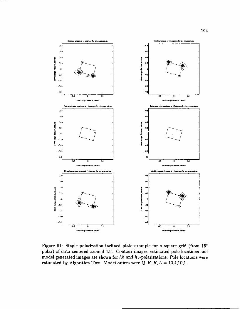
194
Coto- -Wm 15 dgv for hh-pol-Mo Contow mir 115 delgr.. for h-polanzb*o
0.8 0.8
0.6 06-
j 0.4- 0.4
0.2- 0.
0 0
-0.2 -0.2.0.4 -0.4-
-0.6 -0.6
-0.8 -0.8_
-0.5 0 0.5 -0.5 0 05
crarn distance meten-com-age d~stmoo., meteos
Estimated pole locaboi at 15 degn. for hh-polanzabon Edtoed pole locatons a 15 &p.tes for hv-polorinbot
0.8 0.8-
0.6 0.6-
0.4- 0.4-
0.2 0.2
-0.2 I-02. , -042g -0.4 I -0.4
-0.6 -0.6
-0.8 -0.8-
-0.5 0 0.5 -03 0 0.5
orc.-rnge diamoo, merm -- ran g dnaim. mee
Model lleneted oogr .t 15 degre for hh-polnmbatmo Moe&] genrtld n at 15 deg.. for hv-pohno.6on
0.8 0.8-
0.6- 0.6
0.4- 0.4-H H
0 0
I-0.2 -0.2
-0.4 --0.4
-0.6 -0.6
-0.8 -0.8-
-0.5 0 0.5 -0.5 0 0.5
mange dost-n, metem -g, duhmwe, m
Figure 91: Single polarization inclined plate example for a square grid (from 150polar) of data centered around 150. Contour images, estimated pole locations andmodel generated images are shown for hh and hv-polarizations. Pole locations wereestimated by Algorithm Two. Model orders were Q, K, R, L = 10,4,10,1.
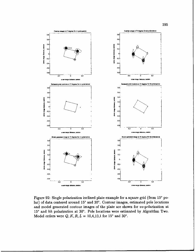
195
Ctopt wu t 15 ISegr fr v-potusmba Cewtos mv at 30 deg. fm. hb-pohmmhba
0,8 0.8
0.6 0.6
0.4 0.4-
02 0.2
S 0 j 0
-0.2 -0.2
-048 -0.8
-0.5 0 0.5 -03.5 0 0.5
aon-sms d. me- dutmses mokrs
Etimat-d pole Ioch0 at 15 &pg.e f. w-poitaiw1 EgUtstad pole tocstb. at 30 &g s~o for hh-polrmustt
0.8 0.8
0.6 0.6
0.4- 0.4
-0.2 -0.2
-0. 1-0.4
-0.6 -0.6
-0.8 -0.8
-0.5 0 0.5 -0.5 0 0.5
ModeI genm ed unage at 15 dcgre for w-polinio Mod.1 pm..trd g-WA = t 30 dqm for hh-phtmn.t
0.8 0.8
0.6- 0.6
04 1 0.4
0.2 0.2-I I10 0-
1 -0.2 -0.2
-0.4 -0.4
-0.6- -0.6
-0.8 -0.8-03.5 0 0.5 -0.5 0 05
mro .-t d , meter. w-t-ng. dtw. m r
Figure 92: Single polarization inclined plate example for a square grid (from 150 po-lar) of data centered around 150 and 30'. Contour images, estimated pole locationsand model generated contour images of the plate are shown for vv-polarization at150 and hh polarization at 300. Pole locations were estimated by Algorithm Two.Model orders were Q, K, R, L = 10,4,10,1 for 150 and 30' .
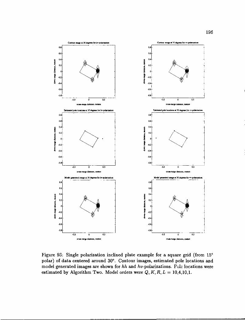
196
Contotu toat 30A for hv-ponero Contou wt a . 30dW- f-- .mlazttm
0.8 0.8j
0.4 0.6
0.2 0.2
-0.2 -0.2
-0.4 -0.4-
-0.6 -0.6
-0.98 -0.8
-0.5 0 0.5 -0.5 0 05
org-rao &ttmoe, t or-rgom dwtsncc, ment
atimated pole boations at 30 dogre fo hv-po4nhmbo EtAted pole lomm at 30 l eea for .v-polanot sbr
0.8 0.8
0.6 0.6
0.4 0.4
0.2 I 0.2
100S-0.2 -0,2
-0.6 -0.6
-0.8 -0.8
-0.5 0 0.5 -05 0 0-5
'orm-nnge dwtatn, mte- ora-aqngo dtan dm
Model gatoated onage at 30 damea for hv-polerinoot Modlel p m at tage .130 degrees for w.h nmon
0.8 0.8-
0.6 0.6-
0.4- 0.4-
0.2 o
10 0-
-0.2 -0.2-
-0.4 I -0.4-
-0.6 -0.6-
-0.8 -0.8-
-05 0 0.5 -0.5 0 0.5
orwataSe ditae, moton mra.- ge dunoto, mtew
Figure 93: Single polarization inclined plate example for a square grid (from 150polar) of data centered around 300. Contour images, estimated pole locations andmodel generated images are shown for hh and hv-polarizations. Polc locations wereestimated by Algorithm Two. Model orders were Q, K, R, L = 10,4,10,1.
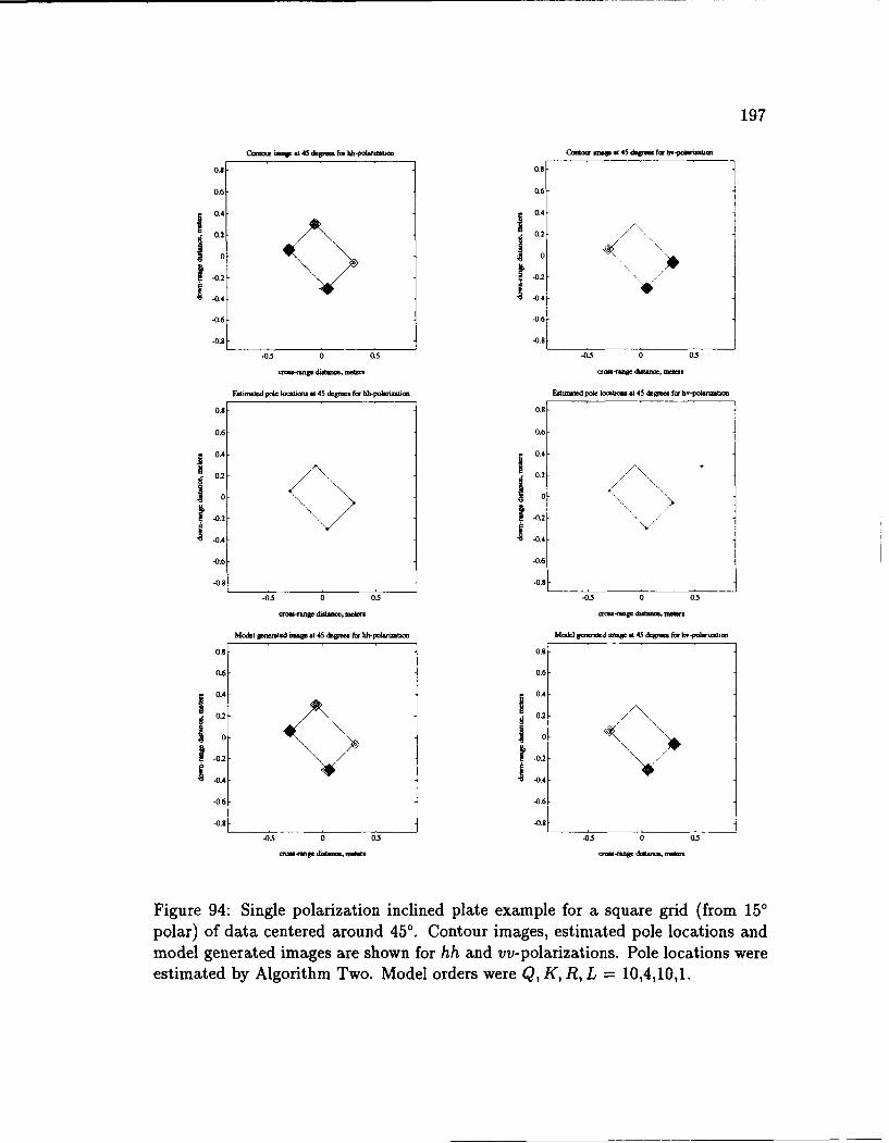
197
Camt= .ua at 45 rg, for hh-oi..pmbsm Ct m at 45 dtg. for hv-pomud=
0.8 0.8-
0.6 0.6-
0.4- 0.4Soi- 0.2 /'",
10 10
-0.2 -01
-0.4 -0.4--0.6 -0.6-
-0.8 -0.8
-03 0 0.5 -0.5 0 0.5
crm-@me ditwme, mveln oum*-ange d Ju-6 .b-
Estimatod pock loc¢ n m at 45 depmes for hh-polizativ Estmted pok loon at 45 degr for hv- polian
0.8 0.8
0.6 0.6
0.4- 0.4
10 10
, -0.2 -0.2
-0.4 - 0.4
-0.6 -0.6
-0.8 -0.8
-0.5 0 0.5 -0.5 0 0.5
Model 8eawted uaWga 45 &e. for hh-poL1i on Model generated Wmp 45 dqpm for hv-polfnr=bon
0.8 09
0.6- 0.6
0.4 0.4-
0.2 -0o2
I4-~-0.4- -. 24
-0.6- -0.6-
-0.8 -0.8-
-0.5 0 0.5 -0.5 0 0.5
- did-, M erm-wanga do itji, .n
Figure 94: Single polarization inclined plate example for a square grid (from 150polar) of data centered around 45'. Contour images, estimated pole locations andmodel generated images are shown for hh and vv-polarizations. Pole locations wereestimated by Algorithm Two. Model orders were Q, K, R, L = 10,4,10,1.
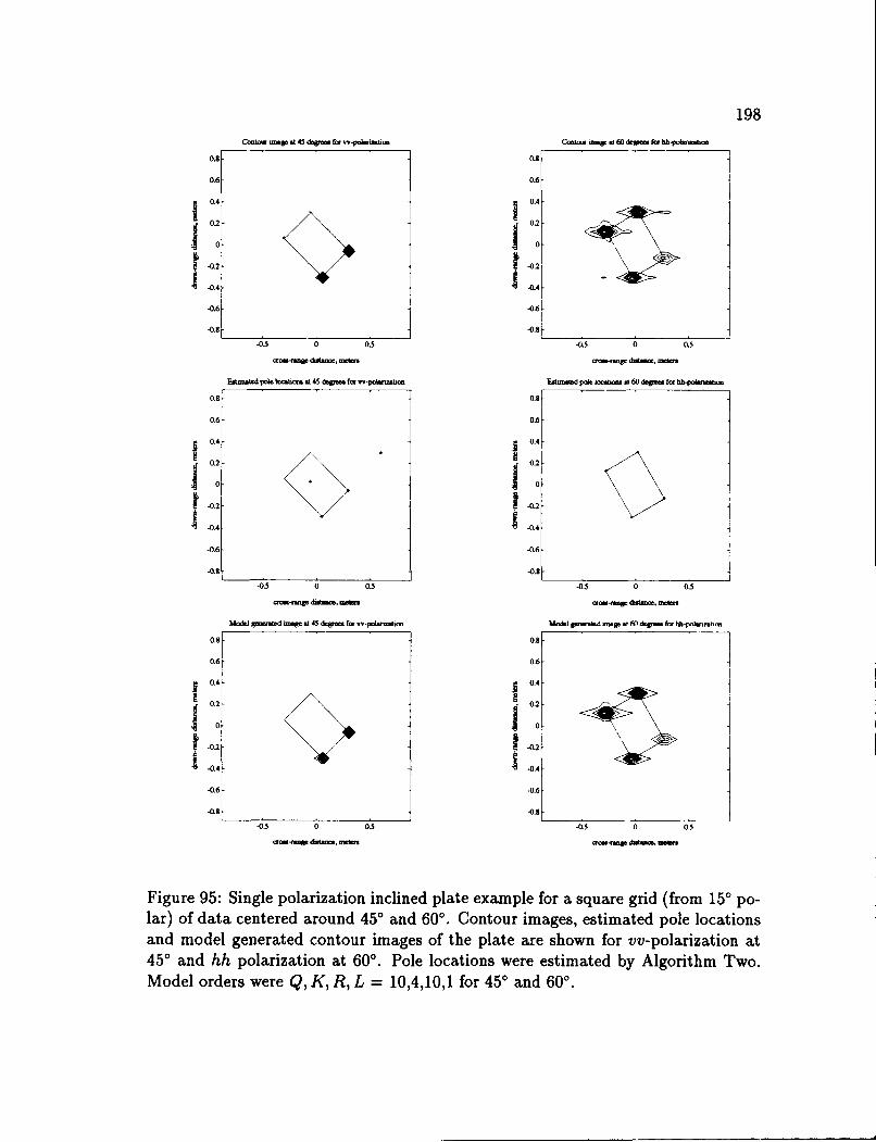
198C-o- .p .145 cl-mss for v-pohmzbtb C sms.e : .60 d.U. for lh-polmabo
0.8 0.8
0.6 0.6
0.4- 0.4-
0.2 . 0.2
0 0-0.2 -0.2
-0.4 -0.4
-0.6 -0.6
-0.5 0 0.5 -03 0 0'3
~mmftd poe. lo ad45 degme t f.por l. Ed-m ipole poodeon s 60 dpm for hh-poacua.
0.8 0.8-
0.6 0.6-
0.4 j 0.4
0. 0.2
100-0.2 -02-
1 -0.4- -0.
-0.6 -0.6
-0.8 0.8-
-0.5 0 03 -03 0 0.5
arm-w tmnom , maim ornsno dwuwoe, metere
Model Venrted un&F at 45 dagezes for vv-pol~bm Model genertted -Wa wt 61 &V-tl ke hhj 4-"-hn
0.8 0.8
0.6 0.6
0.4 - 0.4
.2 10.2i 0 0
-0.2 -0.2
-0.6 .0.6
-0.8 -.0.8
-0.5 0 05 -05 0 03
aos.-ri d- -. metem dro-a te noaf
Figure 95: Single polarization inclined plate example for a square grid (from 150 po-lar) of data centered around 450 and 600. Contour images, estimated pole locationsand model generated contour images of the plate are shown for vv-polarization at450 and hh polarization at 600. Pole locations were estimated by Algorithm Two.Model orders were Q, K, R, L = 10,4,10,1 for 450 and 600.
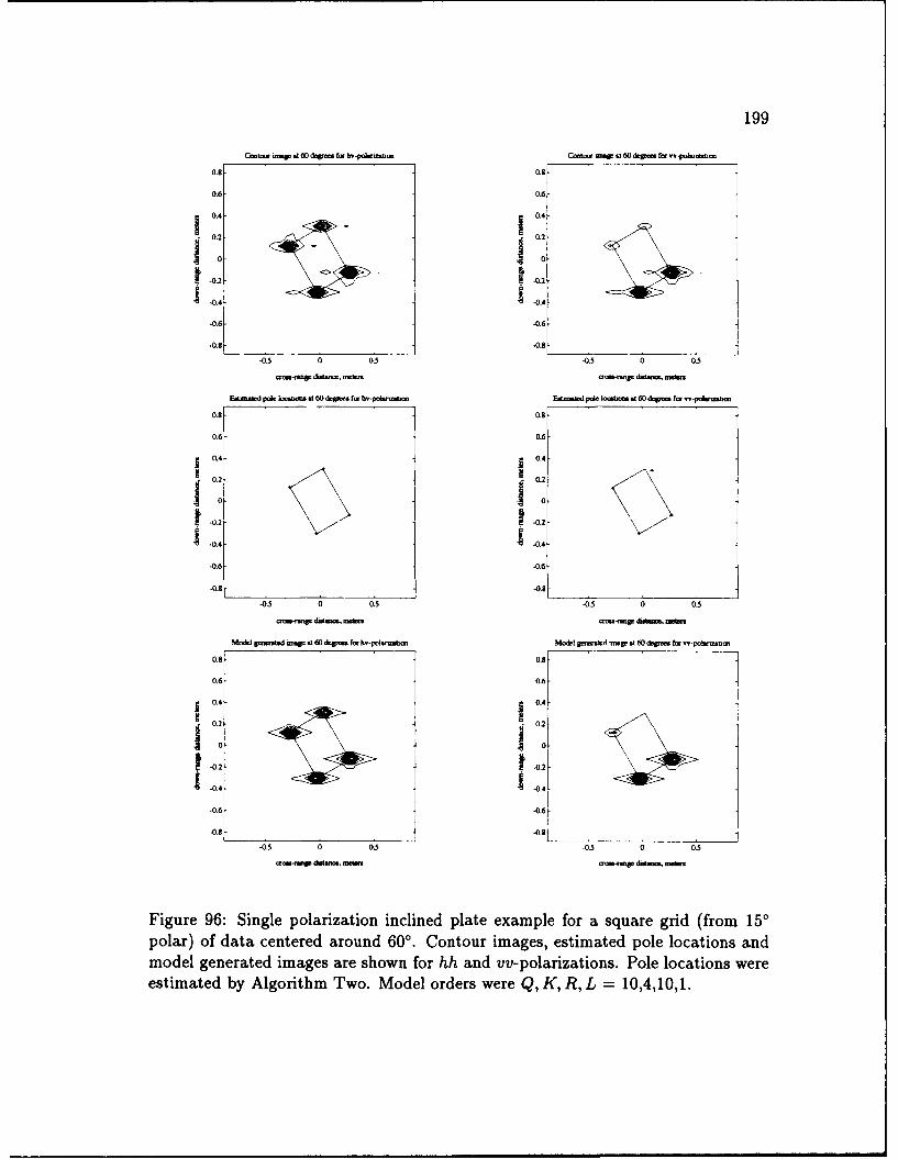
199
Catmo -60 dqm ~f bv-poIwmza. C x O .60 dp.. f. n-ploumu
0.8 0.8
0.6 0.
0.4
-06 -0.
-0.8 -048
-0.5 0 0.5 -0.5 0 05
-mnp dt ~, me.. -rp~ dimc wm'
Eitm.A-d pole locsb= at 60 dagi.4 fm hv-poi.n.uon E-Aund poe Iodb at 60 4
., fm vv-pokr=nM=
0.8- 0.8-
0.6 0.6-
0.4-j 0.4-
0.2 8o0i-
10 j 0[1 -0.2
-0.6- -0.6
-09- -0.8
-05 0 05 -0.5 0 05
c'o-rui d2nm, mnet -m dume rdms
Mo w* gzmted map at 60 &rV.. fm hv-poknramh Model ga.k-t mow .160 g. ftr w-To
0.8 08-
0.6 0.6-
0.4- 0.4-
0.2 0.2
1 0 -0
-0.2-.
-0.4 -41-0.6 -0.6-
-0.8 -0.8
-05 0 0.5 -0.3 0 0.5
Figure 96: Single polarization inclined plate example for a square grid (from 150polar) of data centered around 60'. Contour images, estimated pole locations andmodel generated images are shown for hh and vv-polarizations. Pole locations wereestimated by Algorithm Two. Model orders were Q, K, R, L = 10,4,10,1.
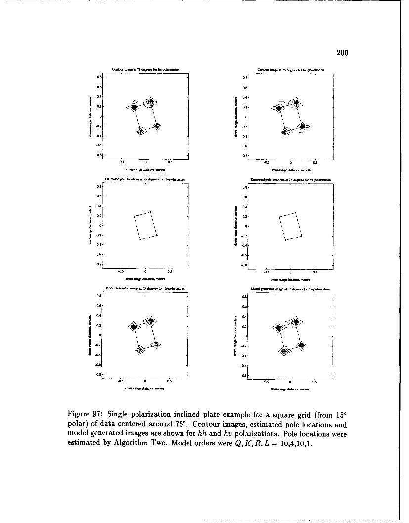
200
C-U- ..p at 75 d w far hh-ohab G mfl a75de for v-pWlar~bm
08 0.8
0.6 0.6
02.4 0.20 0
100-0.25 -0.2
.04 0.4-06 -06
-08 .5.03 0 0.5 -05 0 03crc-vm dos= meun €:owge Ast mcn
Etmied p-k Ioobru w 75 dt~me. fa h-polmbn E.m1ve-d pole lobtmt t 75 dg- fc h.pokna.e
0.4- 0.8
0.2- 0.6
OA 0" 0.4-
.00.2
.04- -0.4
-0.6- -0.6
.0.8 -0.8
-0.5 0 0.3 -0.5 0 0.5
arf-n ge dw.ono metr caa -n~e diao meur.
Model amemtd mW st 75 ft fa. hh-pohunnm Model goessld mp at 75 deicg for Iw-pohn-mum
0.8 0.8
0.6 0.6-
0.4- 0.4-
01- 1
.02 1 o.-0.4-1 -04,
.0.6 46
.0.8 -0.8
-0.5 0 0.5 -0.5 0 0.5
Figure 97: Single polarization inclined plate example for a square grid (from 150polar) of data centered around 75'. Contour images, estimated pole locations and
model generated images are shown for hh and hv-polarizations. Pole locations wereestimated by Algorithm Two. Model orders were Q, K, R, L = 10,4,10,1.
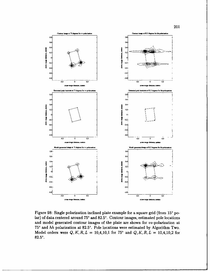
201
Contour =W at75 dagnms for v.-pdlan-on Clemo., =W at82.5 &paaaa hb-pahnj
0.8 0.8-
064 0.6-
0 0
-02 - 0.2
-0. 1.0.4-0 6
-06-0.8 -0.8
-0.5 0 0.5 -0 0 0.5
aosranga dlao. mede daoaag taot. Owers
Eglougetd pole loostons at 75 degrees for - polaroo Eaum...d pole tloounsa 9123 dagee.t for hh-poarnbm
0.8 -0.8-
0.6 0.6-
I 0.4- 0.4-
02 0.2
101-0.2 1-0.2
-0.6 -0.6
-0.8 -0.6-
-0 .5 0 0.5 -05 0 0.5
aes-rage dutaoe. nalm ooaa.ege -~m amser
Modl geerated oreage at 75 degrees for -poltniban Model genratd Unag a 912-S degreas fer bhr-polarnatoee
0.8F 0.8-
0.6 0.6-
j0.4 j0.4
0.2 0.2
10 10
S-0.2 1-0.21.0.4 1a .-
-0.6- -0.6-
-0.8. -0.8-
-05 0 0.5 -05 0 0.5
creap dtatance. inatr atrange dr.Wm invie.;
Figure 98: Single polarization inclined plate example for a square grid (from 150 polar) of data centered around 750 and 82.5'. Contour images, estimated pole locationsand model generated contour images of the plate are shown for vv-polarization at750 and hh polarization at 82.50. Pole locations were estimated by Algorithm Two.Model orders were Q, K, R, L = 10,4,10,1 for 75' and Q, K, R, L = 10,4,10,2 for82.50.
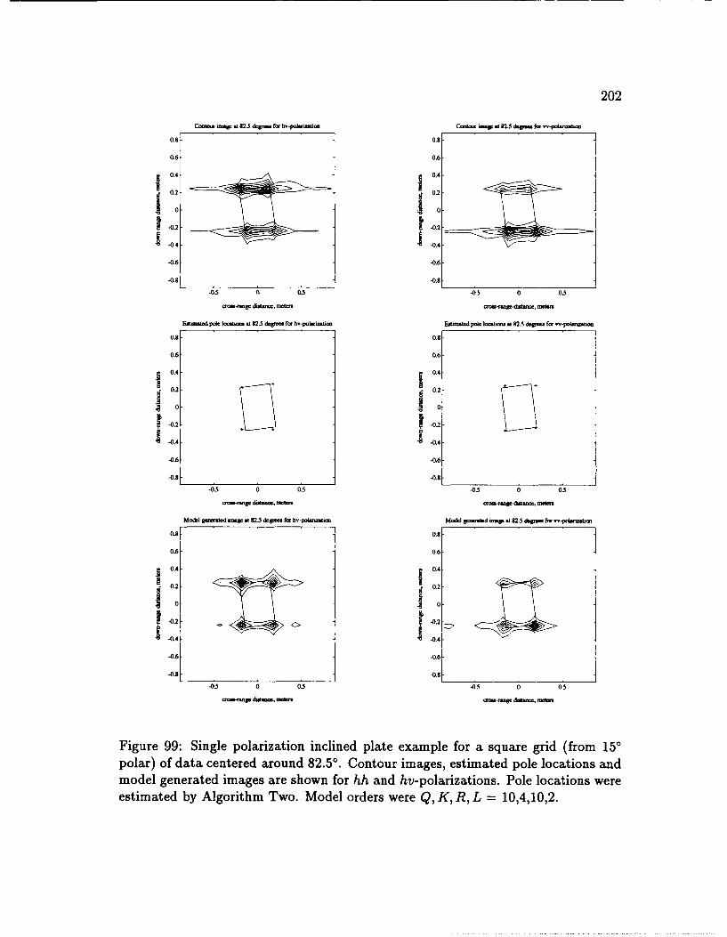
202
Cotog am t 82.5 degee fo hv-pol nwim C.= .. v .1825 &qp. f. o-polnum
0.8 0.8
0.6 0.6
I 0.4 0.4-
0.2 0.2
0 0
-0.2 -01
-0.4 .0.4
-0.6 -0.6
-0.8 -0.8
-0.5 0 03 -05 0 0.5dio.-r .m 3ot, m rW dwms m ,cb mcbm
Eetnnad pole locsbto at 825 degreel fm hv-polritolnr EAm&d pcle locrho 91825 degree. for w-pokrU
0.8 0.8
0.6 0.6
0.4- 0.4
0.2 3 0.2
0 0
0-0.2- -01
-0.4- -0.4
-0.6- -0.6
-0.- -
0.8
0 0 0 05-0 0 0
a-mvo d goe mcom~ am-ong dw-on. rekne
Modl p-ateed Iloege 12.5 degwe fbr Rw-poholtio MM Fpwed ,mrw a823 degees f., -polunbo
0.8- 0.98
0.6 0.6
04 ~ .- Kj0.4-
0.0.20 US-0.42 -0.4
-0.6 --0.6
-0.8- -0.6
-05 0 05 -0.5 0 05
or-fop damlee, moe, "=- , mm
Figure 99: Single polarization inclined plate example for a square grid (from 150polar) of data centered around 82.50. Contour images, estimated pole locations andmodel generated images are shown for hh and hv-polarizations. Pole locations wereestimated by Algorithm Two. Model orders were Q, K, R, L = 10,4,10,2.
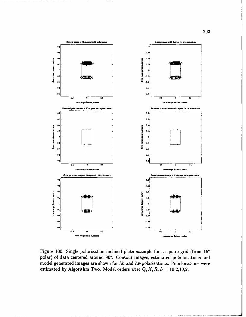
203
Cwtawm unaa*90dogmc fbh-polsmb= Cwi a1.*9Opgwfm. b-pokrnsbm
0.8 0.8
0.6 0.6
0.4- 0.4-
021 0.2
10 710-. 24 1 20
-06 -064
-0.6 -0.8-
-08 -0 .5 0 0.5 -. 8 -0.5 0 0.5
crm-rs dwmt.e, n.b=r asm~p dwtno mekrs
E..tmnated pole Ioc.0 at 90 degioc (y hh-polarmt= FtonOkd pciloca aort 90 dgoo fm hv-pohrimb
0.9- 08-
0.6- 0.6-
0.4- 0.4-
0.2-0.2
-0.2 1-02
1-04A -0.4
-0.6 -0.6
-0.8 ___________________ 1-0.8-0.5 0 0.5 -0.5 0 0.5
Model gen.Wud 90.. Odpgr eor hh-olmabo Model 8F.d o. v w 90 &eUo f.r hv-PolwOb
0.8- 0.8-
0.6- 0.6-
0.4- 0.4-
-0.2- 0.2
1-0.2- -0.24:-0.6- -0.4
-0.6- -0.6
-0.5 0 0.5 -0.5 0 0.5
oru.ood,.awo, meteo daimco, meft.
Figure 100: Single polarization inclined plate example for a square grid (from 150polar) of data centered around 900. Contour images, estimated pole locations andmodel generated images are shown for hh and hv- polarizations. Pole locations wereestimated by Algorithm Two. Model orders were Q, K, R, L = 10,2,10,2.
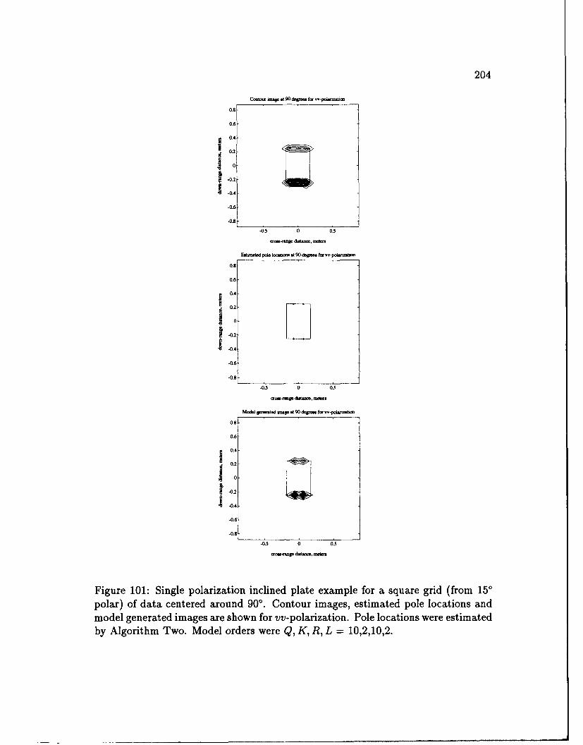
204
0.8-
0.6-
I0.4-0.2-
0-
-. 2
.0.4
-0.6
-0.4
-0. -002
0. -0.
-0.6-
-0.4-
-0.0002
-0.4
-0.6
-0. 040
0.2-
.4-
-0.2
-0.8
-0.5 0 0.5
Figure 101: Single polarization inclined plate example for a square grid (from 150polar) of data centered around 90'. Contour images, estimated pole locations andmodel generated images are shown for vv-polarization. Pole locations were estimatedby Algorithm Two. Model orders were Q, K, R, L = 10,2,10,2.
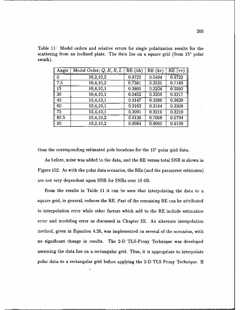
205
Table 11: Model orders and relative errors for single polarization results for thescattering from an inclined plate. The data lies on a square grid (from 150 polarswath).
Angle Model Order; Q, K, R, L RE (hh) RE (hv) RE (vv)
0 10,2,10,2 0.9722 0.5494 0.97227.5 10,4,10,2 0.7381 0.3531 0.718915 10,4,10,1 0.3805 0.3204 0.359330 10,4,10,1 0.3452 0.3206 0.321745 10,4,10,1 0.3147 0.3286 0.362060 10,4,10,1 0.3163 0.3164 0.330875 10,4,10,1 0.3091 0.3219 0.321082.5 10,4,10,2 0.6126 0.7008 0.679490 10,2,10,2 0.9084 0.9090 0.9130
than the corresponding estimated pole locations for the 15' polar grid data.
As before, noise was added to the data, and the RE versus total SNR is shown in
Figure 102. As with the polar data scenarios, the REs (and the parameter estimates)
are not very dependent upon SNR for SNRs over 10 dB.
From the results in Table 11 it can be seen that interpolating the data to a
square grid, in general, reduces the RE. Part of the remaining RE can be attributed
to interpolation error while other factors which add to the RE include estimation
error and modeling error as discussed in Chapter III. An alternate interpolation
method, given in Equation 4.26, was implemented on several of the scenarios, with
no significant change in results. The 2-D TLS-Prony Technique was developed
assuming the data lies on a rectangular grid. Thus, it is appropriate to interpolate
polar data to a rectangular grid before applying the 2-D TLS Prony Technique. If
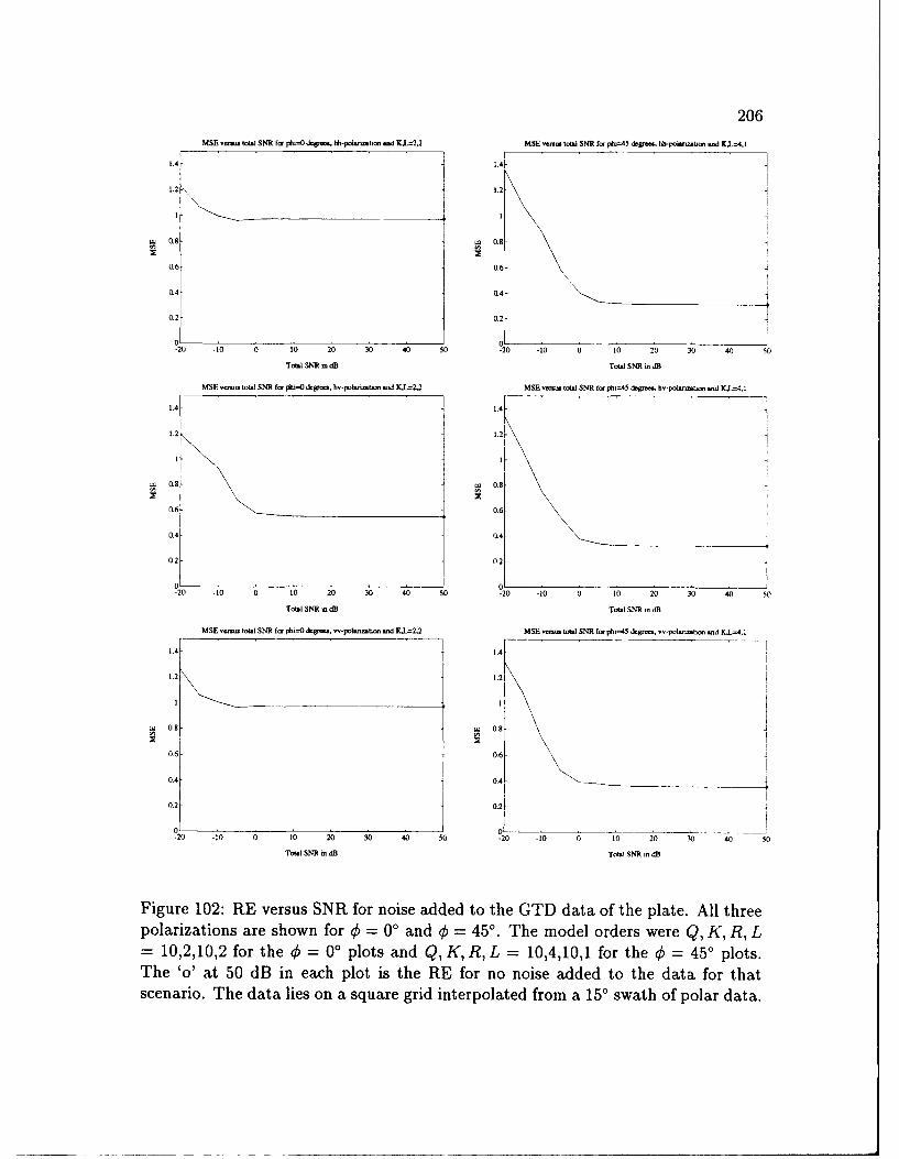
206MSE in.total SNR for phxu0 dea hl,-polan-.tim. .. d KL=2,2 ?dSE vemus total SNR for *b.
45 degmin. hhpolaiza. ... KL=41
1.4- 1.4-
1.2 1.2
LU 0.8 W 0.8-
0.6 0.6
0.4 0.4-
0.2 0.2-
01 0-20 -10 0 10 20 30 40 50 -20 -10 0 10 20 30 40 50
Total SNR m. dB Total SNR odB
MSEvo.o total SNR for pi=() d&os, hp-roaal,. and K.L-2,2 MSE -ux total SNR fg phitAS &grin hv-polanzt o and KL=4.l
1.4 - 1.4 -
1.2- 1.2
.o 0.8 to 0.8
0.6 0.6
0.4 0.4
0.2- 0.2-
J 0-20 -10 0 10 20 30 40 s0 -20 -10 0 to 20 30 40 50
Total SNR mdB Total SNR dBA
MSII -a.. total SNR for pi-O0 &g& o-pol.-h~ton and K.L=2,-2 MSE -aat total SNR for pioo45 &grot, v-polatio and KL=41~
1.4- 1.4-
1.2- 1.2-
to 0.8- to 0.8 4
0.6~ 0.6
0.4 0.4 _________
0.2 0.2
-20 -10 0 10 20 30 40 so -20 -t0 0 10 20 3 40 s0
Total SNR aAdB Total SNl .n dB
Figure 102: RE versus SNR for noise added to the GTD data of the plate. All threepolarizations are shown for 4) = 00 and 4) = 45'. The model orders were Q, K, R, L= 10,2,10,2 for the 4) = 00 plots and Q, K, R,L = 10,4,10,1 for the 4) = 450 plots.The 'o' at 50 dB in each plot is the RE for no noise added to the data for thatscenario. The data lies on a square grid interpolated from a 150 swath of polar data.
207
the angular swath of the polar data is small, this step may not be necessary, and
interpolation error can be avoided. The next data set, analyzed in Section 6.3.4,
confirms this assumption for a 30 swath of polar data.
6.3.4 Single Polarization Analysis of Three Degree PolarSwaths of Data
In order to determine if the angular extent of the data set has a significant effect
on the RE and the parameter estimates, a new data set was generated. This data
set is also 31 x 31, but the angular extent is only 30 with samples every 0.10, while
the frequency range is from 9.0 GHz to 9.48 GHz in 0.016 GHz steps. Figures 103
through 116 show the simulation results for this scenario. Shown for each angle
are three contour images of the plate, each image corresponding to one of the three
polarizations, found by directly using the polar data in the 2-D IFFT. Also shown are
three sets of pole locations, each set corresponding to one of the three polarizations,
estimated by Algorithm Two with no noise added to the original data. In the cases
where there are more than four poles, only the four highest energy poles are shown in
these plots. Along with these plots contour images are shown which were generated
from all of the estimated parameters (not just the four highest energy poles). The
parameters estimated by Algorithm Two are used in the 2-D model in Equation 5.2
to generate data in the 2-D frequency domain. The unambiguous range, R, is 9.3684
meters in each direction for this data set. Only one-fifth of this range is shown in
each direction in the figures which follow. The model orders were chosen to reflect
the expected number of scattering centers on the plate for the corner dominated
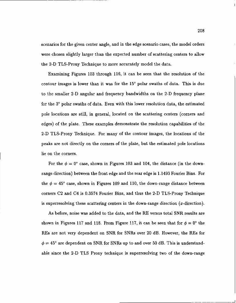
208
scenarios for the given center angle, and in the edge scenario cases, the model orders
were chosen slightly larger than the expected number of scattering centers to allow
the 2-D TLS-Prony Technique to more accurately model the data.
Examining Figures 103 through 116, it can be seen that the resolution of the
contour images is lower than it was for the 150 polar swaths of data. This is due
to the smaller 2-D angular and frequency bandwidths on the 2-D frequency plane
for the 30 polar swaths of data. Even with this lower resolution data, the estimated
pole locations are still, in general, located on the scattering centers (corners and
edges) of the plate. These examples demonstrate the resolution capabilities of the
2-D TLS-Prony Technique. For many of the contour images, the locations of the
peaks are not directly on the corners of the plate, but the estimated pole locations
lie on the corners.
For the 4, = 00 case, shown in Figures 103 and 104, the distance (in the down-
range direction) between the front edge and the rear edge is 1.1493 Fourier Bins. For
the 4, = 450 case, shown in Figures 109 and 110, the down-range distance between
corners C2 and C4 is 0.3574 Fourier Bins, and thus the 2-D TLS-Prony Technique
is superresolving these scattering centers in the down-range direction (x-direction).
As before, noise was added to the data, and the RE versus total SNR results are
shown in Figures 117 and 118. From Figure 117, it can be seen that for 4, = 00 the
REs are not very dependent on SNR for SNRs over 20 dB. However, the REs for
4, = 450 are dependent on SNR for SNRs up to and over 50 dB. This is understand-
able since the 2-D TLS Prony technique is superresolving two of the down-range
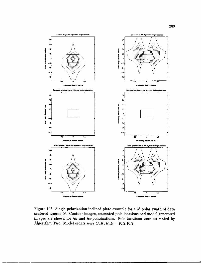
209
Cwt=o infuW At 0 &OO. fmr Whpo1.m.6.. CUote -- p .t0 dop.. for k-pdn.
0.8 0.8
0.6 0.6
02 0.2
0
1-0.2 -1
-0.6 -0.6
-0.6 -086-0.8- -0.9-
-0.5 0 0.5 -0-5 0 0.5aoa-m distain, -tr ma-roan dtota- -
F timated po locatio s at 0 deg ree. for hh-polan _nm Etimad poi lotio n at 0 dou... for hv-poah at=c.
0.8 0.8
0.6 0.6
j 0.4- OA 0
0- 0
-0.4- -0.2
o. i o.10 10
-0.2 -0.2
-0.6 -0.6
-0.8 -0.8
-0.5 0 0.5 -0.5 0 0.5
=rsx-nmu diot .,meter cr-rangedwt-, metes
Modal gecrated monge at 0 deg,.a for hh-polomnbo. Modl garurabod mnge at 0 depe.. for hv-pokwumb.
0.8 0.8
0.6 0.6
0.4 j 0.4
0.2- 01
0- 0
-0.2 - -0.2
1-0.4-1 -0.4/
-0.6 -0.6-
-0.8 -0.8
-05 0 0.5 -0.5 0 0.5mm-rtigo disaws.e mfte -- Wra-m~ ht~..Iara
Figure 103: Single polarization inclined plate example for a 3' polar swath of datacentered around 00. Contour images, estimated pole locations and model generatedimages are shown for hh and hv-polarizations. Pole locations were estimated byAlgorithm Two. Model orders were Q, K, R, L = 10,2,10,2.
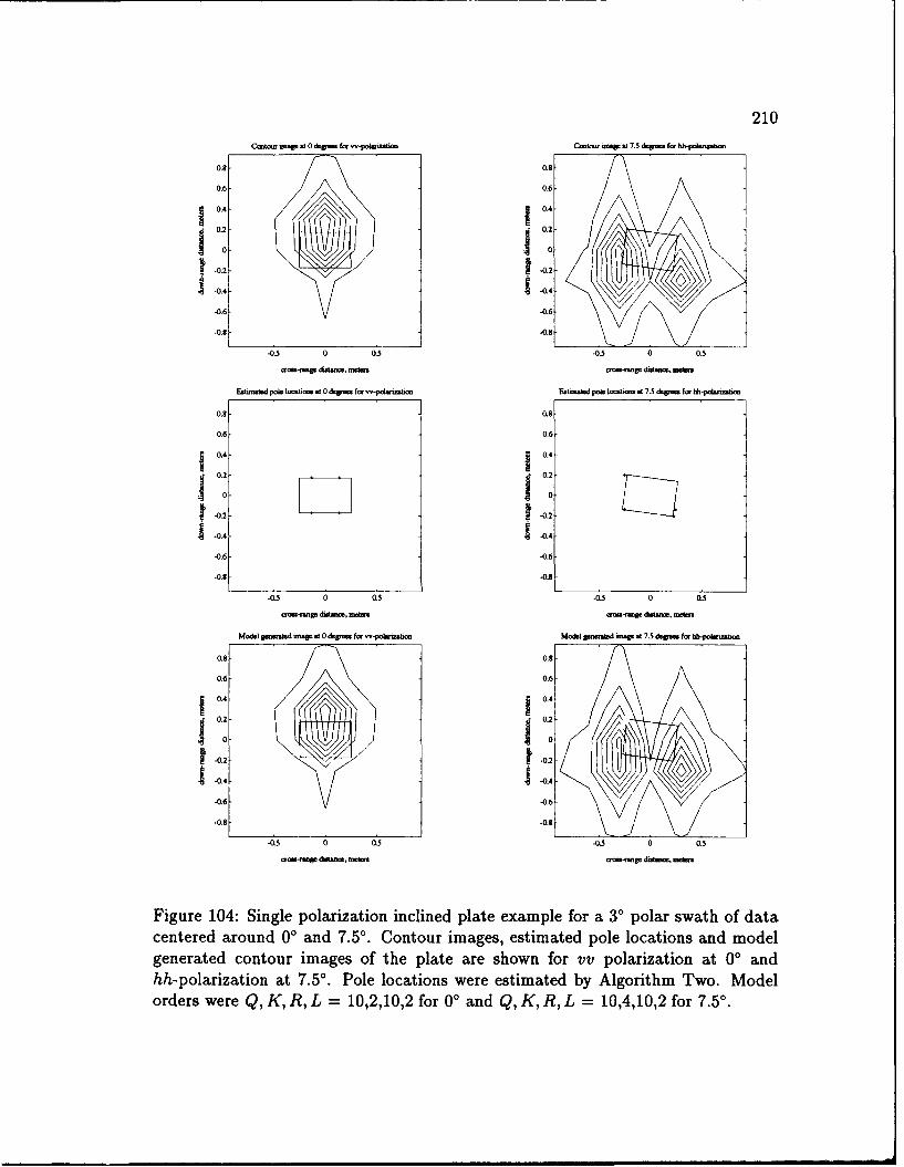
210
Canto unW at 0 dcp for -polaw1Z. Cmoo, WIW @17.5 &. for hh-lb, dlrmto
0.8 0.8
0.6- 0.6
0.4 0.4
0. 0i
-0.2
1-0.4 1-0.4-0.6 -0.6
-0.8 -0.8
-03 0 0.5 -0.5 0 0.5
crfogc diaio, Meanao s-mgr iduo mewe
Esthmald pole locaton at 0 dtgn-tx for w-pdlanzam E~marhed pok loo homt .17.5 de for hh.-polanzaon
0.8 0.8
0.6- 0.6
I 0.4-j 0.4-
0.2 j0.2-0.2 -0.2
1-0.4 1-0.4-0.6 -0.6
-0.8 -0.8
-0.5 0 0,5 -0.5 0 0.5
orm-w diahnce, mders ao-nr dwtswc mer
Model geeurled mqoe t g0 lgs for w-polkrmamhon Model gmeodod ante at 7- dega forpW=U
0.8 0.8-
0.4 0.41.4 0.2
1 0 0o-0.4 -0.4
0.6 -0.6
-0.9 -0.8
-0.5 0 0.5 -0.5 0 0.5
or1-1U18o dutanoc. meter oegndtm h
Figure 104: Single polarization inclined plate example for a 30 polar swath of datacentered around 0' and 7.50 . Contour images, estimated pole locations and modelgenerated contour images of the plate are shown for vv polarization at 00 andhh-polarization at 7.5' . Pole locations were estimated by Algorithm Two. Modelorders were Q, K, R, L = 10,2,10,2 for 0' and Q, K, R, L = 10,4,10,2 for 7.50 .
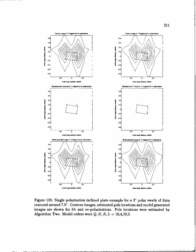
211
Cwtsw - .17.5 d.~m for hv-pohartnlux CIaltotir t15153at.75 deses for v-planoatio
0.8 0.8
0.6 0.6-,\
I 0.4 0.4-0.2 - 0.2
0 0
-0.2 -0
-0.2- -0.4
-0.6- -0.6
-0.8 -0.8
-0.5 0 as -0.5 0 0.5
Eatie5 pole ]-im at u.7.5 dgrsc for hv-pdian0oo E.0zn.Ad poleIts i at 7.5 de. for sw-polininb5
0.8- 0.8
0.6- 0.6-
j 0.4 0.2
0 0-0.2 -0.2
-0.2 -0.2
-0.'6 -0.6
-0.8 -0.8
-0 . 0 0.5 -0.5 0 0.5
or .ge distiinot, 155115. 0-51W datiasor, in
Model g-mle~d 60535 at 7.5 degi for ho-p orshon Modelri o151d u..g at 7.5 d Imr s-polinibon
0.6- 0.6- A
0. J 0 4-,-
0.2 V01
10 10S-0.2 -0.2
I 0.4 I-0.4-0.6 -0.6
-0.8 -0.8
-0.5 0 as -0.5 0 (15
orrsedwigor.mo noo-. dwig.ore, s
Figure 105: Single polarization inclined plate example for a 30 polar swath of datacentered around 7.5'. Contour images, estimated pole locations and model generatedimages are shown for hh and vv- polarizations. Pole locations were estimated byAlgorithm Two. Model orders were Q, K, R, L = 10,4,10,2.
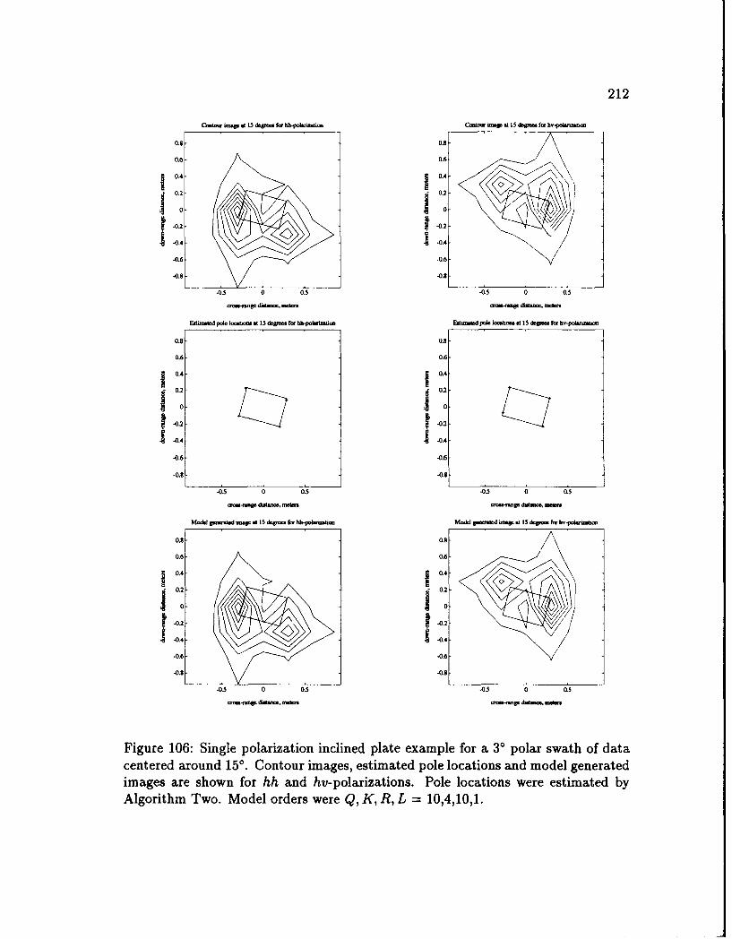
212
Cord1oo amat .15 degor for hh-polannoor' Cow-a at .~15 is &g for h-ol-n
0.8- 0.8-
0.6- 0.6
j 0.4- 10.40.2-0.2
-0.2- 01-1-0.4- -0.4
-0.6- -0.6-
-0.8 -0.8-
-0.5 0 0.5 -0.5 0 0.5
S-mnge datece acb O OO dlgdlor, ane
EAtubtd pole loogimr at 15 clegioro for hb-polanid polo lomornat s15 dqpm. fmr ho-poonuban
0.8 -0.8-
0.6- 0.6-
j 0.4-j 0.4-
0.2 0.2
0 10
-0.2 -0.2
10A 1-0.4-0.6 -0.6
-0.8 0.
-0.5 0 0.5 -0.5 0 0.s
Model gen~mtd usap at 15 dcgroo for hb-polwona Model Snwased oor at15 dcgor for b-polauioba
0.8- 0.8 /
0.6- 0.6
J 0.4-j 0.4
0.2 - 0.2
-0. -0.2/
-0.4 0.4-
-0.6 -0.6-
-0.8 -0.8.
-0.5 0 05-0.5 0 aLSor~U-1OgO M00.. 0o U~o-~opdMwoor an.e
Figure 106: Single polarization inclined plate example for a 30 polar swath of datacentered around 15'. Contour images, estimated pole locations and model generatedimages are shown for hh and hv-polarizations. Pole locations were estimated byAlgorithm Two. Model orders were Q, K, R, L = 10,4,10,1.
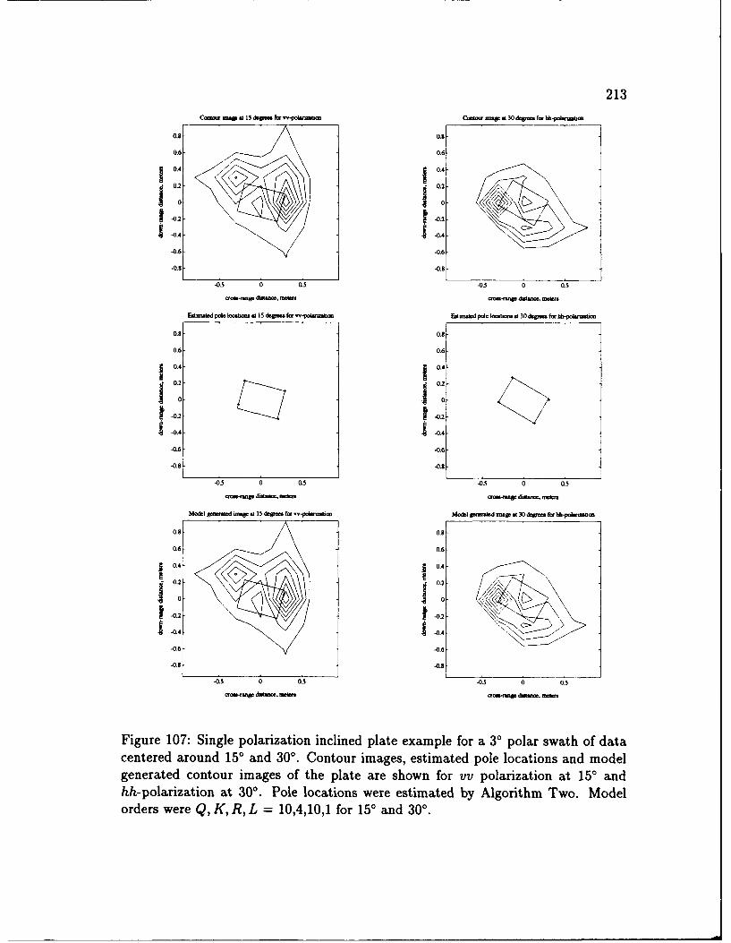
213CmlRw .unlp at 1s dee for av-poer-mbian CoN nU at 30 dwm f. nvnh=mU
03- 0.3
0.6 0.6
I 04 2 0.4
0 0
-0. -0.6
-0.8 -0.8
-0.5 0 05 -0.5 0 asos-p duua , nwm -- Wn dwtm, -W.
Eat pole ocao at 15 dogre. for -- pola m Esalmaed pole kotir ost 30 degree for hh-polseutmon
0.8 0.8
0.6- 0.6
-0.4 -0.4
1 0.2 0.2
0 10
.0.2 -0,2
-0.4 -0.4
-0.6 -0.6
-0.8 -0.6
-0.5 0 as -0.5 0 0.5
q Sraoe diatanw, mlenu 0.r=nge dautce, man
Model g eword imWge st 1gres 1 fm r-polamo Model pns.hd unag .130 degres for hh-poleezmo
0a 0.
0.6- 0.6-
I 0.4 1 0.40 0
-0.6 -0.6
-0.3 -0.4
-0.s 0 0.s -0. 0 0,5
-e danance. mrew. om.nne dtanu mese
Figure 107: Single polarization inclined plate example for a 30 polar swath of datacentered around 150 and 300. Contour images, estimated pole locations and modelgenerated contour images of the plate are shown for vv polarization at 15' andhh-polarization at 300. Pole locations were estimated by Algorithm Two. Modelorders were Q, K, R, L = 10,4,10,1 for 15' and 300.
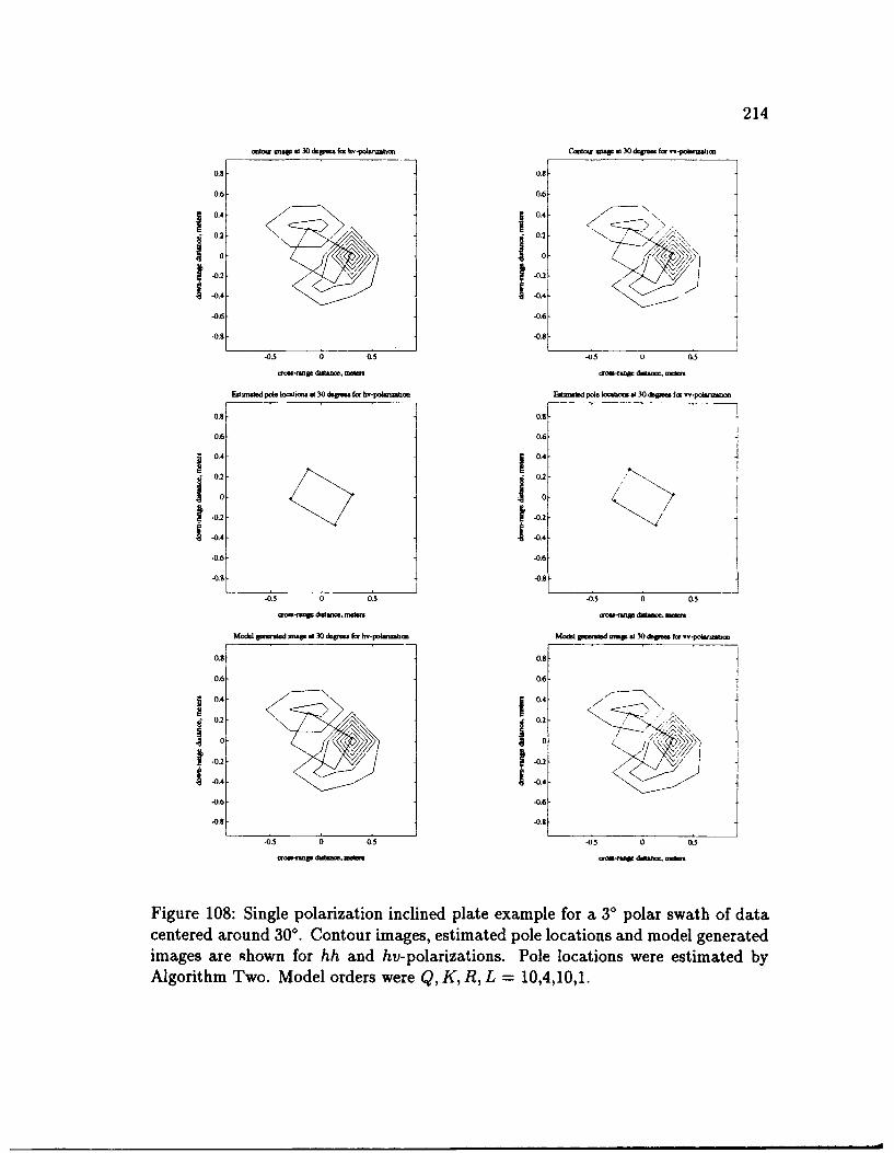
214
mk)tO mop at 30 dep, for k-poWtsnm Call=A -se at M Sowp for or-poIlnai.m
0.8- at9[
0.6- 0.6-
j 0.4 j0.4-
0.2 -0.2-
-0.62 -. 6-
-0.8 j -0.8-
-0.5 0 0.5 -0.5 0 (13
or.-.pdtda, o re osenp deelnc, mem
Eieoetod pok lomttcns at 30 deg e for hv-poWLantzm Eied pole 1,6m. at 30 .kg, for -pombo
0.8 10.9-0.6- 0.6,
j0.4-j 0.4-
0 0-0.2 -0.2-
.0.4 1-0.4--0.6 -0.6-
-038 -0.8-
-0 .5 0 as3 -0.5 0 0.5
ao-fun dawnm. mebt, aonp daimme. wm.
Model guseabcd -p at 3 0
d~m for liv-pot-nm, Model pmenftd u..p at 3 0
dp, fir -epotashm
0.6 0.6-
J 0.4 j0.4
0.2 0.2
0 I~10
. -0.42- -0.4
-0.6 -0.6-
-0's -0.8
-0.5 0 0.5 -0.5 0 (Is
aowrmpe dwtre.mtr ores- dw ma
Figure 108: Single polarization inclined plate example for a 3' polar swath of datacentered around 300. Contour images, estimated pole locations and model generatedimages are -;hown for hh and hv-polarizations. Pole locations were estimated byAlgorithm Two. Model orders were Q, K, R, L = 10,4,10,1.
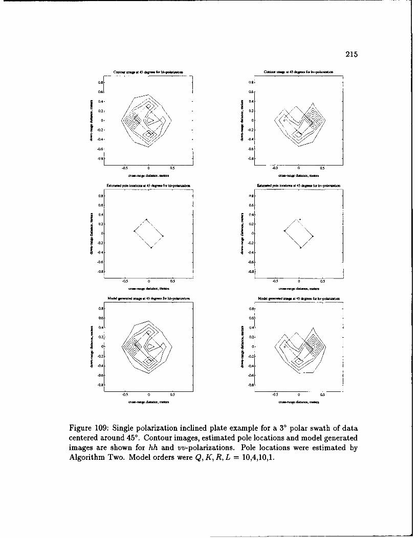
215
C~al- map .14 d ~ f. hh-polmuaba Caou map @145 degm f4 hbpoknz.1m
0.8- 0.8-
0.6- 0.6-
j 0.4-<~ 0.4-
0 §j< 0\ \ 2
-0.2 01.
44 -0.4 .77. -ON
-0.6 -0.61
-0.8 L-0.8-0.5 0 0L5 -0.5 0 0.5
Eg,,~a.1d pole bca at 45 dtg.. fmi hh-poklabm EstnnO~d pole locnbid .45 dqp fm hv.pobuizgbm
0.8-
0.6- 06.
0.4- 04j 0.2 - 0.2 -
-0.2 ~ -01
-0.4-N - -0.4
-0.6- -0.6.
-0.8- -0.8-
-0.5 0 (05 -0.5 0 0L5
M.&I g-w~Ud upt .45 dqpm~ fm hh-pw*.6o Mocki Sw..d im at 45 ... fa bv-po. nb
0.8- 0.8-
0.6- 0.6-
j 0.4-j 0.4-
S0.2-.7 0.2 /
0-0 0 \
S-0.2 -- 01
I -0.4 1-0.4-0.6 -0.6
-0.8 -0-. 3-0.8 -. .
-o r. 0 ' e 0s -03 , 0w - (5
Figure 109: Single polarization inclined plate example for a 3' polar swath of datacentered around 450. Contour images, estimated pole locations and model generatedimages are shown for hh and vv-polarizations. Pole locations were estimated byAlgorithm Two. Model orders were Q, K, R, L = 10,4,10,1.
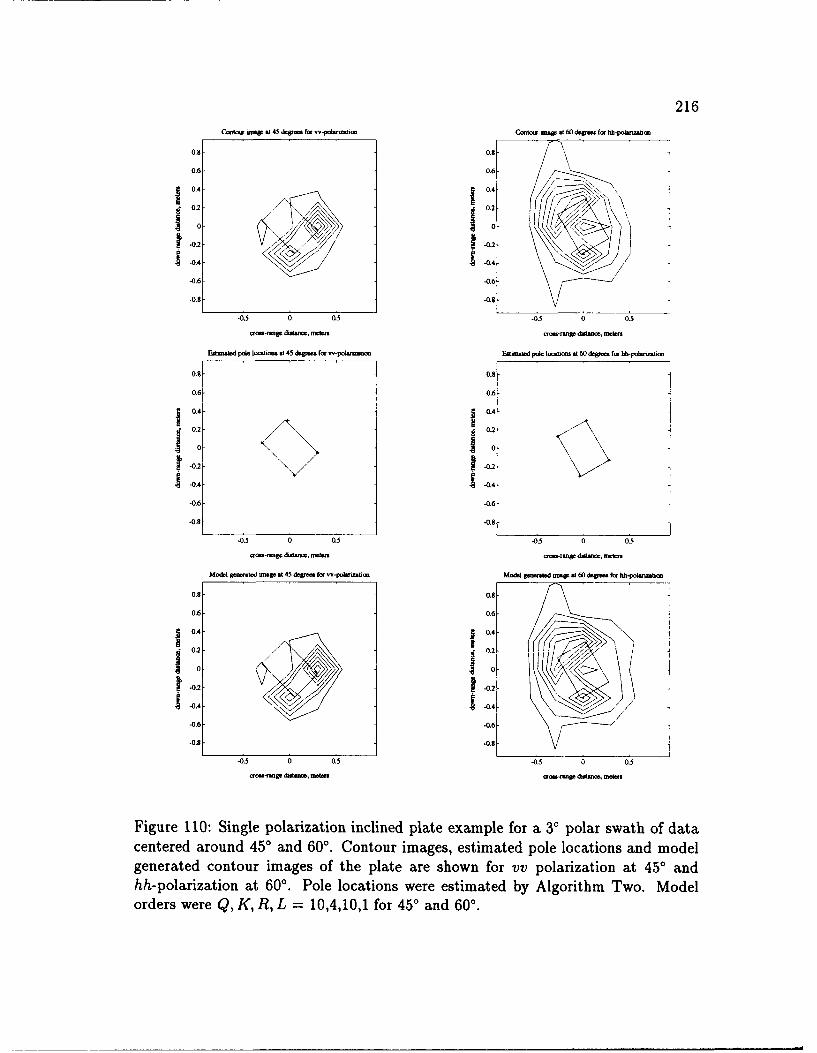
216Guto umV A 45 degr fbt v.poirmbt CImu miW at 60 degt fm hh-pol.mi
0.8 0.8-
0.6 0.6
04- .4/0.2 / 0.2
0--0
-0,6 -0.6
-0.8 -0.8
-0 5 0 0.5 -0.5 0 0.5
crang dawe, mea 'r-pn dance, mc
EstImtied poIe locStaom at 45 dagt s for w-po6-st-n Estatcd poIe Wlbocslist at 60 dC m fo hb-poInati
0.8 0.8
0.6 0.6
I 0.4-j 0.4
0.2 0.2
I 0 0
-0.2 -0.2
-0.4 .1 -0.4
-0.6 0.6
-0.8 -0.8
-0.5 0 0.5 -0.5 0 0.5
o -ge dw mete -- d t-c nub
Model genaWed umna at 45 ddWfor kx -potwsrmlot ModW pnmw.d ttttw .6 d.gves for hh.n-b.n
0.8 0.8-
0.6 0.6-
0.4- 0.4-
0.2 (.2
0a 00o 1 o
-0.2- -0.2-Ic
-0.4- -0.4/
-0.'6- -0.6-
-03 0 0.5 -0 5 0 0.5
Figure 110: Single polarization inclined plate example for a 30 polar swath of datacentered around 450 and 600. Contour images, estimated pole locations and modelgenerated contour images of the plate are shown for vv polarization at 450 andhh-polarization at 600. Pole locations were estimated by Algorithm Two. Modelorders were Q, K, R, L = 10,4,10,1 for 45' and 600.
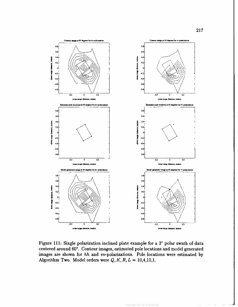
217
Ccotmff ua at 60 dope fix hv-oaimiz &mtoa, m. t 60 dejp for -- pohnueam
0.8- 0.6
0.6 062
10 10
-0.2 -K)10.2
-0.4- -0.4-
-0.6- -0.6-
-0.8- -0.9
-0.5 0 0as -03 0 0s
Estad poIk kxsbccs mi 60 dmg. for hv-polar mxhi Egtm,.*d pok Io.oo at60 dcg,. fo, vv-pola
0.8 1 0.8
0.6- 0.6-
j 0.4- 0.4-
,j 0.2- 0.2
0- 0-0.2- -02
-0.4-- -0.4
-0.6 -0.6
-0.8 0.
-0.5 0 0.5 -0.5 0 0.5
Model geo-ted unoW at 60 depe- for hv-polau60 Modl Soaled lp at 60 dkpga fm~ -polwzift
0.6- 0.6-
j 0.4 0.4-
al 0.2-
-0.2 9-0.2 ---0.4- -0.4-
-0.6- -0.-
-0.8- -0 .8
-0.5 0 0.3 -05 0 as
Figure 111: Single polarization inclined plate example for a 30 polar swath of datacentered around 600. Contour images, estimated pole locations and model generatedimages are shown for hh and vv-polarizations. Pole locations were estimated byAlgorithm Two. Model orders were Q, K, R, L = 10,4,10,1.
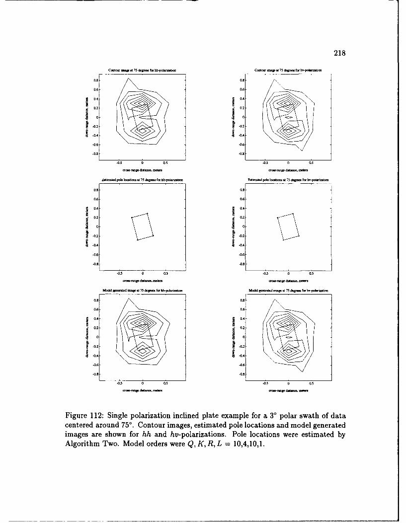
218
Contar umep st 75 dtlmo fo' hh-potizantat Contoor -Wa at 75 d&. for hv-pola n
0.8 0.8
0.6- 0.6
10.4 104S0.2 - 02
0 0
-0.2 -0.2
,-04 0.4--0.6 -0.6
-0 8 -0.8
-0.S 0 05 -0.5 0 0.5
-o-~g. duinte, me am--9.g dot-6 vee
ktt metcd pole 3o0di. st 75 degI.. for bhpolton Ftaim.td pole lombonu at 75 dftm. for hv-poarit.
0.8 0.8
0.6 0.6
0 0.4 - 0.4
0.2 0.28
0 0
-0.2 -0.2
-0.4 -0.4
-0.6 -0.6
-0.8 -0.8
-0.5 0 0.5 -05 0 0,3
&A--ne Jn, mee ' gc -t' n ae nv*.*e
Model gnerated m2W t 75 deg for hh-polmri bn Model 80rdatbd map at 75 dqpw for hv'rRbm
0.8- 0.8
0.6 0.6
0.4 . 0.4
• 0 0
-0.8 -0.8
-0.5 0 0.5 -0.5 0 0.5
.o naw dm- a . -msa~-a. dwxx4 mm
Figure 112: Single polarization inclined plate example for a 30 polar swath of datacentered around 750. Contour images, estimated pole locations and model generatedimages are shown for hh and hv-polarizations. Pole locations were estimated byAlgorithm Two. Model orders were Q, K, R, L = 10,4,10,1.
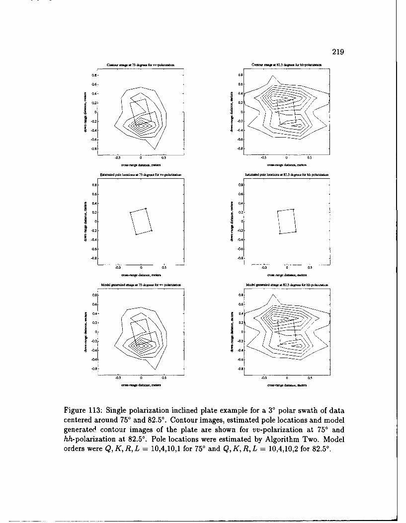
219
on=uW at 75 dWua fmr vvj~o4.nbmor Cuaot zo ax 82.5 &gorra6hh-potanmbma
o 81. 08-
0.6 0.6-
10.4 04
0.2 0.2
10 10
-0.2 0.2
1 -0.4 -0.4--
-0'6 -0.6
-0.8 -0.8
0.6 1 0.6-
0.4-j 0.4-
- 0 . 0
-0.2- -0.2
I-OA - -O.4
-0.6 -0.6
-0.-5 0 0.5 -0.-5 0 0.5
oron-axgt dntau, motor ~ao-g. daw, e- ?~~
?x~d.l gmmxW xxog* at 75 &goo f., 0V- oJ~rzbmx MoM* gRatd oa at 82.5 dgro fm hhjokruab,
08- 0.8j
0.6- 0.6-
0.4- 0.4
0.2 0.2
-0.2 20.:-0.4-.
-. 6 -0.6
-0.8 -0.8 --0.5 0 0as -0.5 0 053
O dO8O 6tOr mt. ~-go &gao, mcko.
Figure 113: Single polarization inclined plate example for a 3' polar swath of datacentered around 750 and 82.50. Contour images, estimated pole locations and modelgenerated contour images of the plate are shown for vv-polarization at 750 andhh-polarization at 82.50. Pole locations were estimated by Algorithm Two. Modelorders were Q, K, R, L = 10,4,10,1 for 750 and Q, K, R, L = 10,4,10,2 for 82.50.
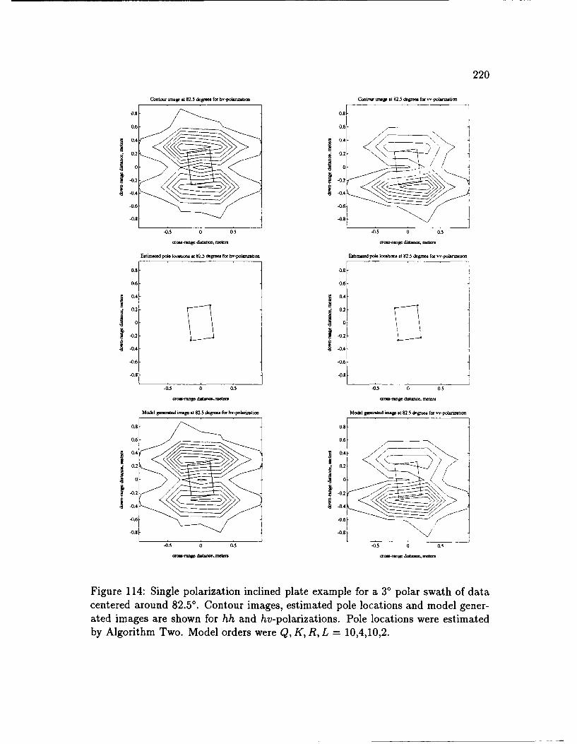
220
Coot., -W. at 2.5 degrate for hv-poltmnmto Corftota, .. Wt 823 deree, for v-.,lO.ueon
0.8 0.8-
016 0.6-
0.4 04-
0. 042
00
S-0.2 1-04.2
-0.8-08
-0.5 0 0.5 -0 0 0)5
c--orngo distanc, itorn orr-ge doosto, teeters
Estunte1 pole to~nori. at 82.5 degre for hiv-pohnomaboo Eshmaled pole locattons at 823 deg-oe for o-potlanIor
0.8- 0.8-
0.6- 0.6-
j 0.4- 0.4-
0.2- 0.2
01
-0.2- -0.2
1-0.4- -0.4 --0.6- -0.6
-0.8- -0.8
-0.5 0 0.5 -0.5 0 05S
Model got.1r.8d .png at 82.5 dag-r for hv-polhizion Model gewoad matle .t1823 degre, for ro-po~ootteot
0.8- 0.8-
0.6 0.6{
1 0- 0.41
0.2 czzz 02-
0-0
-0.2 -.
-04 -0 . 4
-0.6- -0.6-
-0.8 1---0.8 1
Figure 114: Single polarization inclined plate example for a 3' polar swath of datacentered around 82.50. Contour images, estimated pole locations and model gener-ated images are shown for hh and hv-polarizations. Pole locations were estimatedby Algorithm Two. Model orders were Q, K, R, L = 10,4,10,2.
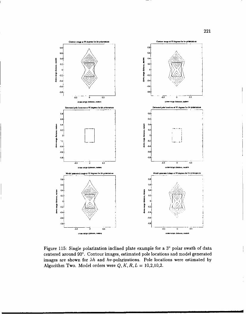
221
Cwtitm.-S 0~ta6.b-owt C,,t.. sW W 90O&0...f hb otM
0.8 0.8
0.6 0.6-
* 0.4 0.4-/
~0.2 /-0.2/
0 0-0.6 -06
-0.4 -084
-0.5 0 0.5 -0 0 0.5
Etmt-t.d po6,le htwnS t 90 dg- f. hh-pOwanztbo F-edttk pole lo.tt.,, t 90 &gm. f. hv-po...U
0.8- 0.8-
0.6- 0.6-
0.4- 0.4-
- 0
I -0.4- -~-0.4
-0.6- -0.6
-0.9- -081
-0.5 0 5 -05 0 0.5
Mock] 9 ~otcd unage at 90 d&g9o fm. hh-pau~a~m MOt&I g.tkd =W~ W 90 dcgto. fbr ho-poIl-Um~o
0.8 0.8
0.6 0.6-/
j 0.4-j 0.4-/
-0. : 5o 0.2 -. _______
-0.6 /-0.6
-0.8 -0.8
-05 0 0. .
Figure 115: Single polarization inclined plate example for a 3' polar swath of datacentered around 90'. Contour images, estimated pole locations and model generatedimages are shown for hh and hv-polarizations. Pole locations were estimated byAlgorithm Two. Model orders were Q, K, R, L = 10,2,10,2.
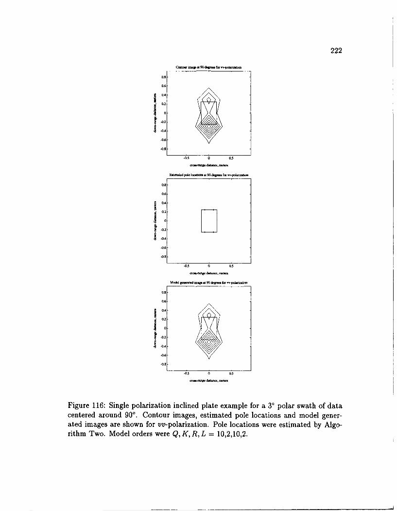
222
0.8-
0.6-
I0.4-- 0.1
-u01-024
-0.'6
-0.8
-0 .5 0 053
-rn8 dutano. m
E*sa&d pot lomfia at 90 depan fa w-onz.1m
0.8
0.6-
-0.2
10-0.2
I-0.4-0.6
-0.8
-0.5 0 0.5
aos-fifge duwa , meb=t
Moddl gwasta unqa at 90 degs for -poainbio
0.8-
0.6-
I0.4-0,2
10
I-0.2I -0.4
-0.'6
-0.8
-0.5 0 0.5
c dw-f , 8u . . t
Figure 116: Single polarization inclined plate example for a 30 polar swath of datacentered around 900. Contour images, estimated pole locations and model gener-ated images are shown for vv-polarization. Pole locations were estimated by Algo-rithm Two. Model orders were Q, K, R, L = 10,2,10,2.
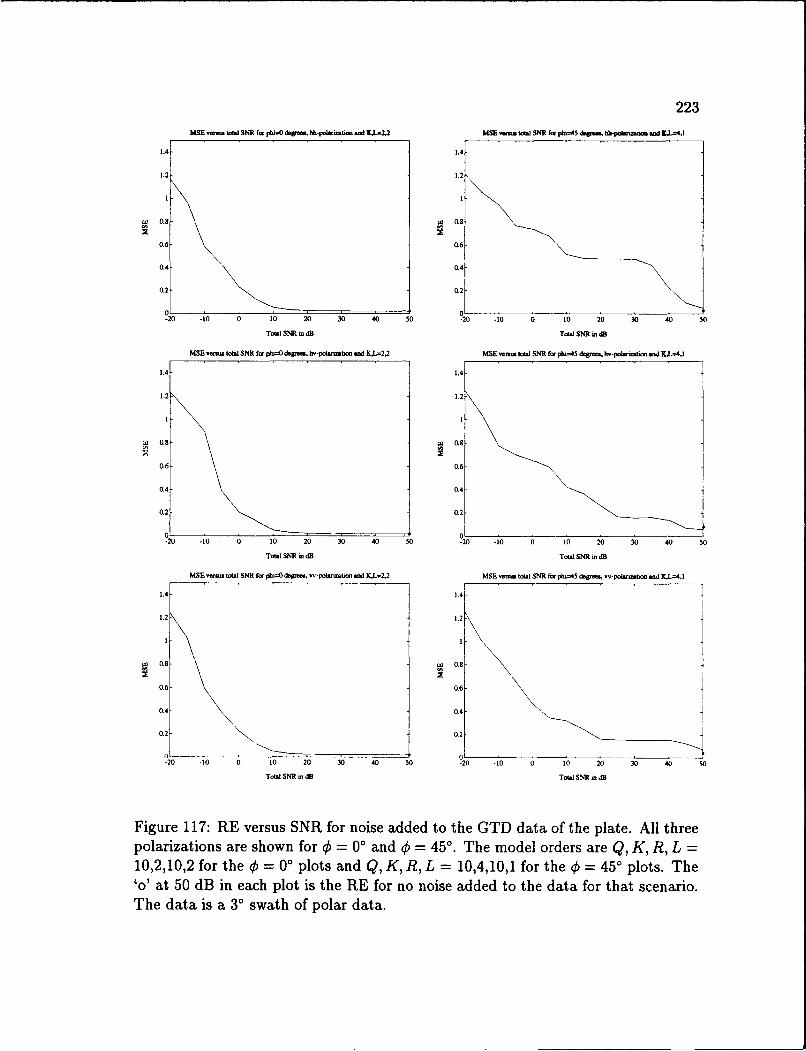
223
MSE vama total SNR fa ph0 a, hh-polarmtin aid K.jL2.2 MSE msut tAW SNR fi pla=45 dai. bh-pahan wd LJL ,1
1.4- 1.4-
1.2 1.2
W 0.8 0.8
CL6 -0.6-
0.4 ( -
0.2- (0 .2
-20 -10 0 10 20 30 40 so -20 -;0 0 10 20 30 40 s0
Total SNR ModB Total SNR dB
MSE versu total SNR for pnl=0 degmo, hv-polarmton and KL=2,2 MSE wrtus total SNR ftr pln=45 dtgrae- hv-polaiation and KAL4,1
1.4 - 1.4-
1.2 1.2
0.8- W 0.8
0.6 a6
0.4 0.4
0.2- 0.2
00-20 -10 0 10 20 30 40 50 -20 -10 0 10 20 30 40 50
Total SNR w dB Total SNR in dB
MSE veton total SNR for pbi=O defpma e, w m-polaoton anl KJ.,.2,2 MSE v.ntm total SNR for 45 dpgreea, vv-polaiinnon and Kj..4,1
1.4- 1.4
1.2 1.2
I o
Wo 0.6- no 0.8-
0.6 0.6
0.4 0A
0.2- 0.2
0?20 -10 0 10 20 30 40 so -20 -10 0 10 20 30 40 5
Total SNR m a Total SNR m d
Figure 117: RE versus SNR for noise added to the GTD data of the plate. All threepolarizations are shown for 4 = 00 and 4 = 450. The model orders are Q, K, R, L =10,2,10,2 for the 4 = 0' plots and Q, K, R, L = 10,4,10,1 for the 4 = 45' plots. The'o' at 50 dB in each plot is the RE for no noise added to the data for that scenario.The data is a 30 swath of polar data.
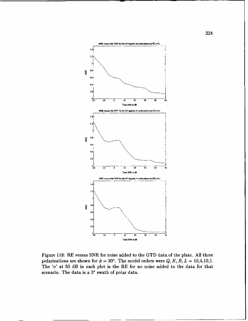
224
MME -a total SNR for *=o30 egras. b~olarat sd XL-o4.1
1.4-
1.2
06
OL4
L2
0-20 -10 0 10 20 30 40 so
Total SNR in dB
MSE -t~o to(.) SNF ft. plu=30 dogroe. bo-poltanoon sod KL=4.1
1.4-
1.2
0.8OS
0.6
0.4-
0,2
0-20 .10 0 10 20 30 40 s0
Told SNR to dB
MSE -o~o total SNR for pltio3O degtos. --ol rhnzort aod K.Lo4,l
1.4-
1.2
Id0.8-
0.6
0.4-
0.2-
0.20 -10 0 10 20 30 40 so
Total SNR tdB
Figure 118: RE versus SNR for noise added to the GTD data of the plate. All threepolarizations are shown for 0 = 300. The model orders were Q, K, R, L = 10,4,10,1.The 'o' at 50 dB in each plot is the RE for no noise added to the data for thatscenario. The data is a 30 swath of polar data.
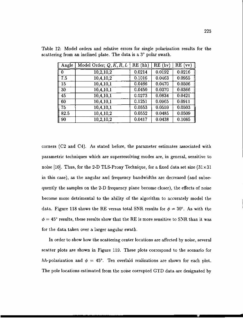
225
Table 12: Model orders and relative errors for single polarization results for thescattering from an inclined plate. The data is a 3' polar swath.
Angle Model Order; Q, K, R, L RE (hh) RE (hv) RE (vv)
0 10,2,10,2 0.0214 0.0192 0.02167.5 10,4,10,2 0.1016 0.0463 0.095515 10,4,10,1 0.0466 0.0470 0.050630 10,4,10,1 0.0450 0.0370 0.036645 10,4,10,1 0.0273 0.0834 0.042160 10,4,10,1 0.1251 0.0965 0.091175 10,4,10,1 0.0553 0.0559 0.050382.5 10,4,10,2 0.0552 0.0485 0.050990 10,2,10,2 0.0417 0.0438 0.1085
corners (C2 and C4). As stated before, the parameter estimates associated with
parametric techniques which are superresolving modes are, in general, sensitive to
noise [10]. Thus, for the 2-D TLS-Prony Technique, for a fixed data set size (31 x31
in this case), as the angular and frequency bandwidths are decreased (and subse-
quently the samples on the 2-D frequency plane become closer), the effects of noise
become more detrimental to the ability of the algorithm to accurately model the
data. Figure 118 shows the RE versus total SNR results for ¢ = 300. As with the
0 = 450 results, these results show that the RE is more sensitive to SNR than it was
for the data taken over a larger angular swath.
In order to show how the scattering center locations are affected by noise, several
scatter plots are shown in Figure 119. These plots correspond to the scenario for
hh-polarization and 0 = 45' . Ten overlaid realizations are shown for each plot.
The pole locations estimated from the noise corrupted GTD data are designated by
226
'+'s while the pole locations estimated directly from the GTD data are designated
by ''s. Six plots are shown, each for a specific SNR between 0 and 50 dB. From
these plots, it can be seen that the location of the corner with the largest scattering
return, which is the left-most corner in the plots (C4), is accurately estimated for
total SNRs as low as 20 dB. As the SNR decreases, the locations of the other corners
are not estimated as accurately. Note that the model orders chosen for this example
were Q, K, R, L=10,4,10,1. These model orders were chosen to reflect the expected
number of scattering centers. The plots corresponding to total SNRs of 20 and 30
dB show that the locations of corners C1 and C2 are not estimated at all. This is
probably due to the closeness of corner C2 to corner C4 in down-range and corner
C1 to corner C3 in cross-range.
This estimation inaccuracy can be corrected for by choosing a larger model order
and retaining the four highest energy poles. This is done, and the results are shown
in Figure 120. The model orders for these plots are Q, K, R, L=10,4,10,2. Only
the four highest energy poles are shown in these plots. From these plots, it can be
seen that the locations of corners C1 and C2 are now estimated by Algorithm Two,
but these locations are not directly on the corners. There is some bias present in
their estimated locations possibly due to the scattering from the other two dominant
corners (C3 and C4) on the plate. However, this example shows that it is appropriate
to overmodel the number of scattering centers when noise is added to data when the
data set chosen requires superresolution to estimate the locations of the scattering
centers.
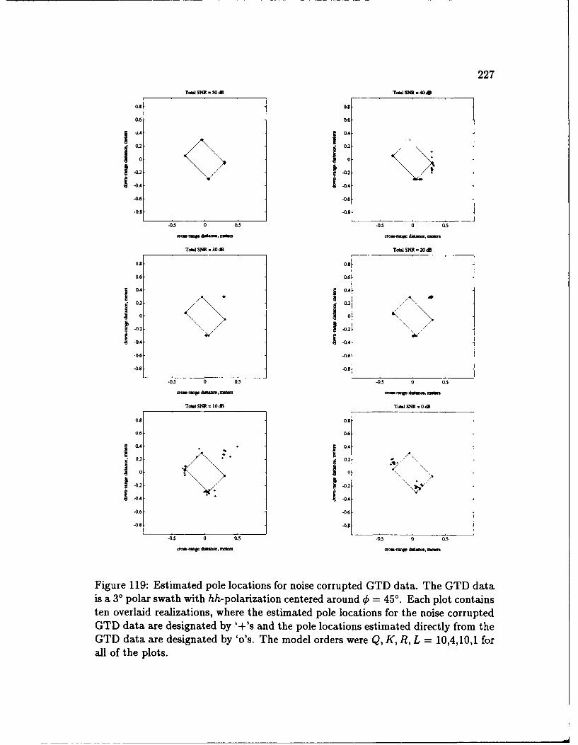
227
Total SM 50 A Total ISk 40 d
0.3 10.0.6- 0.6-
0.4 - 0.4,
1 " 0
.0.2 ~-02
-0.6 -0.6
-0.8 -0.8
-0.5 0 0.5 -0.5 0 0.5
TotalSNR 30 d Total SNR =20 dB
0.3- 0.8-
0.6- 0.6-
0.4-j 0.4-
-0.2 -0.2
-- 0.4 1-0.4-0.6 -0.6
-0.8 -0.8
-0.5 0 0.5 -035 0 (IS
Tota SNR 10 A Total SNR =0dB
0.8- 0.9-
0.6- 0.6-
j 0.4- j 0.4-
0.2- 0.2-
-0.4- -0.4-
-0.6- -0.6-
-0.8- -0.8-
-5 0 0.050 0.5
orsn datmot rnebi orov~ao 4"t tews
Figure 119: Estimated pole locations for noise corrupted GTD data. The GTD datais a 30 polar swath with hh-polarization centered around (k = 45'. Each plot containsten overlaid realizations, where the estimated pole locations for the noise corruptedGTD data are designated by '+'s and the pole locations estimated directly from theGTD data are designated by 'os. The model orders were Q, K, R, L = 10,4,10,1 forall of the plots.
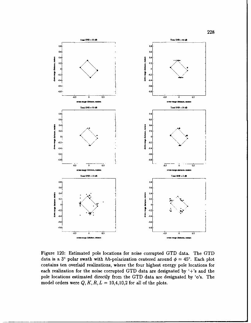
228Tobi SNR = 50dB T,.-SNR=4dB
0.8 0.8
0.6- 06
j 0.4-1 0.4-
-0.2 - -02I -04 1-0.4
-0.6 -0.6
-0.8 -0.8
-05 0 0.5 -0.5 0 as
Totod SNR = 30 dB Tod SNR = 2OdB
0.8 0.8
0.6- 0.6
0.4 J 0.4
0 0
-0.2 \01
S-0.4--0.6 -0.6
-0.8 -0.8
-0.5 0 05 ,-0.5 0 0,5
crm-omi ditobe, r~t1 crob-onb dmm mdm
T.W SNR =10 dB To.W SNR =0dB
0.8 0.8
0.6 0.6-
0.4- 0.4-0.2 "0.2-,
..0 0-
-0/21-0.2
- -0.4 -0.4
-0.6 -0.6
-0.8 ] -. 8
-0.5 0 05 -0.5 0 05
Figure 120: Estimated pole locations for noise corrupted GTD data. The GTDdata is a 30 polar swath with hh-polarization centered around 4b = 45' . Each plotcontains ten overlaid realizations, where the four highest energy pole locations foreach realization for the noise corrupted GTD data are designated by '+'s and thepole locations estimated directly from the GTD data are designated by 'o's. Themodel orders were Q, K, R, L = 10,4,10,2 for all of the plots.
229
From the REs in Table 12 it can be concluded that the 2-D damped exponential
better models the polar data, with no noise added, for data taken over smaller
angular swaths. Even with noise added to the data, for SNRs over 20 dB, the REs
corresponding to the 30 angular swath data are lower than the REs corresponding to
the 150 polar swath data with no noise added. From Figures 103 through 116 it can
be seen that the resolution of the images for a 3' polar swath is less than it was for
the data corresponding to a 15' polar swath. However, the estimated pole locations
are, in general, located on the scattering centers of the plate. This demonstrates the
superresolution capabilities of the 2-D TLS-Prony Technique. This is very useful
since the bandwidth and angular requirements of a SAR are reduced when utilizing
the 2-D TLS-Prony Technique. The angular swath of 30 and frequency bandwidth
of 480 MHz are reasonable numbers for SARs available today. Also, the lower REs
confirm the damped exponential as a valid model for corners away from grazing
angles (see Chapter III).
Several of the 30 polar swaths of data were interpolated onto a rectangular grid
and Algorithm Two was applied to the data (these simulations are not shown here).
In each case, the RE was greater than the REs in Table 12. This larger RE is most
probably due to interpolation error. A drawback to gathering data over a smaller
angular and frequency bandwidth is that the parameters estimated from this data
are more sensitive to noise, as is demonstrated in Figures 117 and 119, than when
parameters are estimated from data gathered over larger angular and frequency
bandwidths. This same characteristic is seen in the full-polarization simulations

230
which follow.
6.4 Full-Polarization Analysis of Plate
The full-polarization data set is now used in FPA2 to better estimate the scattering
center locations and to examine the polarimetric properties of the scattering centers
on the inclined flat plate. As in the single-polarization case, several data sets are
analyzed. First, 150 polar sections of the data are analyzed. Note that as the angle
of incidence changes, the incident polarization changes. Over 15' this may be a
factor. This data is then interpolated onto a square grid and the full-polarization
data is analyzed. Finally, 30 polar sections of the data are analyzed.
The polarimetric characteristics of the scattering centers are represented by po-
larization ellipses calculated from the pole and amplitude coefficient estimates as
discussed in Chapter V. The plotting of the ellipses on the image plane requires
a quantity called the ellipse factor. The units of the amplitude coefficients (which
have the same units of the scattering coefficients, which are the data) are in meters.
This is a result of the definition of the scattering matrix given in Equation 2.19.
Since the coordinates of the image plane are in meters, it is appropriate to place
the ellipses directly on these plots. However, due to the small magnitude of the
scattering coefficients (nominally around 10 - 3 meters), the size of the ellipses must
be scaled-up in order to view them on these plots. Thus, the ellipse factor is the
dimensionless ratio between the size of the ellipses as viewed on the plots which
follow to the actual size of the ellipses.
Note that in Section 3.4 it was stated that separating the angular dependence
231
from the scattering matrix was a poor assumption for canonical scattering centers
such as the corner and the edge. The angular scattering response for the corner and
the edge does vary with polarization, but the impulsive and constant behaviors do
occur at the same aspect angles for the various polarizations. The full-polarization
model in Equation 5.54 is still an accurate representation to the full-polarization
scattering response of a corner or an edge since each polarization has an amplitude
coefficient associated with it. Only the poles, which determine the scattering center
locations, are estimated from multiple polarization data, and each set of amplitude
coefficients is determined from the data set with the polarization corresponding to
that amplitude coefficient. Thus, the full-polarization version of the 2-D TLS-Prony
Technique is a valid full-polarization model for the scattering from ,7anonical scat-
tering centers such as the corner and edge, and using the full-polarization data
simultaneously to determine the scattering center locations and polarimetric char-
acteristics is valid, as demonstrated in this section.
6.4.1 Full-Polarization Analysis of Fifteen Degree PolarSwaths of Data
First, nine 150 polar swaths data are analyzed using FPA2. As in the single polar-
ization analysis for the 15' polar swaths of data the polar data is used directly by
FPA2. The results are shown in Figures 121 through 123. The model orders chosen
reflect the expected number of scattering centers on the plate for the corner domi-
nated scenarios and for the edge dominated scenarios, the model orders are chosen
slightly larger than the expected number of scattering centers. The model orders
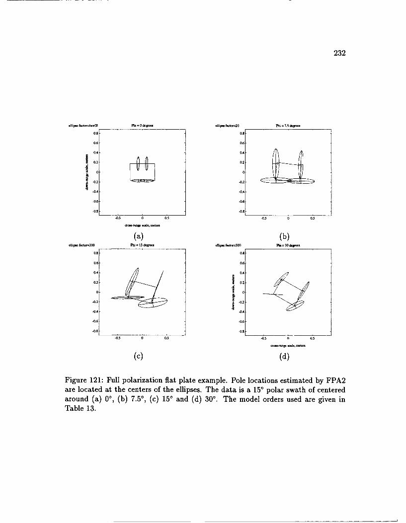
232
.hp. fsdo,=-Iti-0 Phi = 0dpw eh fc --20 Phi = 7.5 & vr
0.8 0.8
0.6- 0.6
0.4 0.4
0.2 0.2
0 0
-0.4 -0.4
-0.6 -0.6
-0.8 -0.8
-0.5 0 0.5 -0.5 0 0,5
croM, rmw e, d
(a) (b)ellipae fctor-200 Phi = 15 degec dhpe fatr--300 Phi : 30 degpees
0.8- 0.8
0.6- 0.6
0.4- 0.4-
0.2 1 0.2
0 0
-0.2 -0.2
-0.4 -0.4
-0.4 -0.6
-0.8 -0.8
-0.5 0 0.5 -0-5 n 05
iemS-emg .ile, ief
(c) (d)
Figure 121: Full polarization flat plate example. Pole locations estimated by FPA2are located at the centers of the ellipses. The data is a 15' polar swath of centeredaround (a) 00, (b) 7.5', (c) 150 and (d) 30' . The model orders used are given inTable 13.
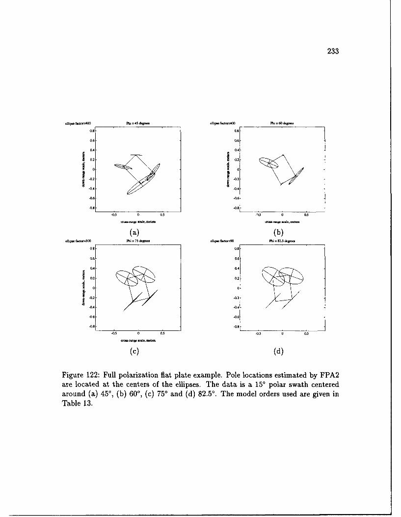
233
ellip fscOv=40 0
Phi = 45 degesm ellpe ftctcrAOO Phi = 60 d&ge i
0.8 0.8
0.6- 0.6
04 0.4
I 0.2 - 0.2
-0. 2 -0.2
-0.4 -0.4
-0.61 -0.6
-0.5 0 0.5 -.L .5 0 0.5
(a) (b)ellipsw factor--30 Phi = 75 dogmes ellipse fada-90 Phi = 82.5 d&g
0,8 0.8
q.6 0.6
04 0.4
I 0.2 0.2
0 0
I -0.2 -0.2
-0.4- -0.4-/
-0.6 -0.6
-0.8 -0.8
-0.5 0 0.5 -0.5 0 0.5
-MV Ic, aete
(c) (d)
Figure 122: Full polarization fiat plate example. Pole locations estimated by FPA2are located at the centers of the ellipses. The data is a 150 polar swath centeredaround (a) 450, (b) 600, (c) 750 and (d) 82.5'. The model orders used are given inTable 13.
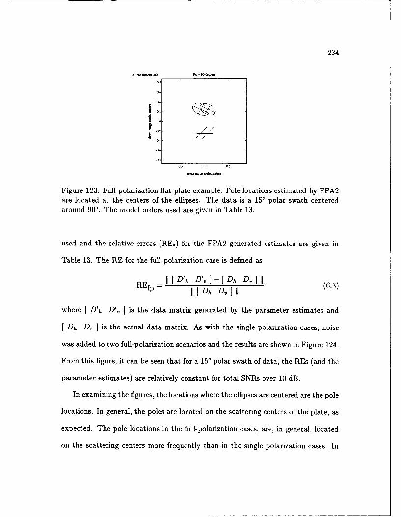
234
.lip. f.1-100 Phi 90 &gM,
0.8
0.6
04
S0.2
-0.2
.0.4-
-0.6
-0.8
-0,5 0 0.5
Figure 123: Full polarization flat plate example. Pole locations estimated by FPA2are located at the centers of the ellipses. The data is a 150 polar swath centeredaround 900. The model orders used are given in Table 13.
used and the relative errors (REs) for the FPA2 generated estimates are given in
Table 13. The RE for the full-polarization case is defined as
R [[[D'h D', ] -[Oh D,,][(.3
11 [ Dh D I, ] 11
where [ Dh D', ] is the data matrix generated by the parameter estimates and
I Dh D,, ] is the actual data matrix. As with the single polarization cases, noise
was added to two full-polarization scenarios and the results are shown in Figure 124.
From this figure, it can be seen that for a 15' polar swath of data, the REs (and the
parameter estimates) are relatively constant for total SNRs over 10 dB.
In examining the figures, the locations where the ellipses are centered are the pole
locations. In general, the poles are located on the scattering centers of the plate, as
expected. The pole locations in the full-polarization cases, are, in general, located
on the scattering centers more frequently than in the single polarization cases. In
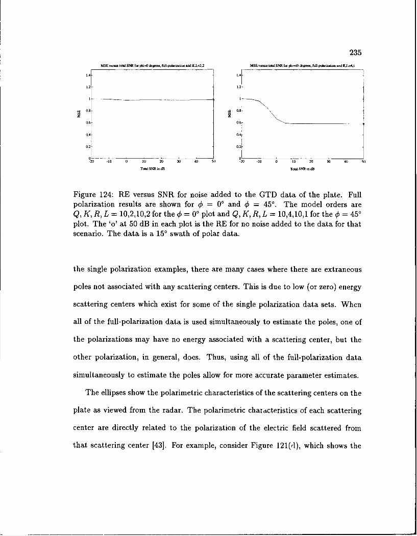
235M SE e.r totl SNR ft phi=O d p .. f.1- pop a.W u d KL=2.2 MSE vt to t SNR fm *u=45 d ~e. c f -p d n ab on . d KjA 1
1.2- 1.4-1..2
1. I.
0.8 ,8 0.8
0.6 0.6
0.4 0.4
0.2 0.20"
-20 -10 0 10 20 30 40 s0 -20 -10 0 10 20 30 40 50
Tot.] SNR dB Tot. SNR dB
Figure 124: RE versus SNR for noise added to the GTD data of the plate. Fullpolarization results are shown for q = 00 and 4 = 45' . The model orders areQ, K, R, L = 10,2,10,2 for the € = 0' plot and Q, K, R, L = 10,4,10,1 for the 4 = 450plot. The 'o' at 50 dB in each plot is the RE for no noise added to the data for thatscenario. The data is a 150 swath of polar data.
the single polarization examples, there are many cases where there are extraneous
poles not associated with any scattering centers. This is due to low (or zero) energy
scattering centers which exist for some of the single polarization data sets. When
all of the full-polarization data is used simultaneously to estimate the poles, one of
the polarizations may have no energy associated with a scattering center, but the
other polarization, in general, does. Thus, using all of the full-polarization data
simultaneously to estimate the poles allow for more accurate parameter estimates.
The ellipses show the polarimetric characteristics of the scattering centers on the
plate as viewed from the radar. The polarimetric chadcteristics of each scattering
center are directly related to the polarization of the electric field scattered from
that scattering center [43]. For example, consider Figure 121(d), which shows the
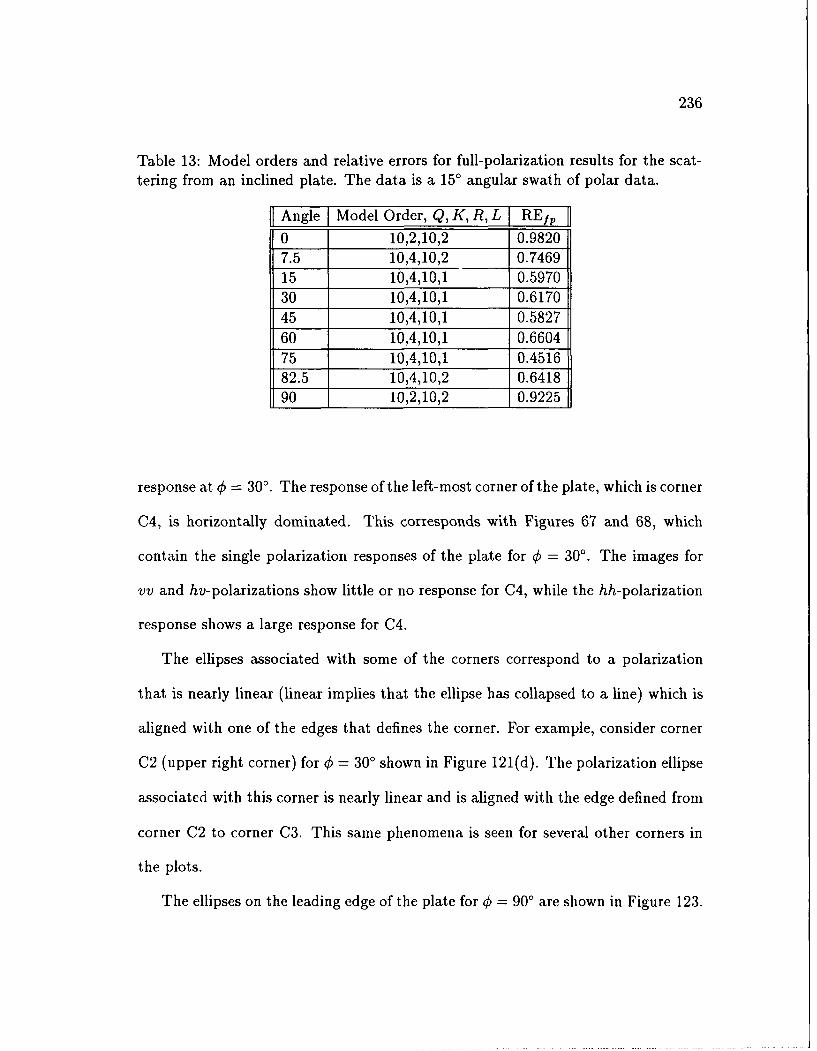
236
Table 13: Model orders and relative errors for full-polarization results for the scat-tering from an inclined plate. The data is a 150 angular swath of polar data.
Angle I Model Order, Q, K, R, L [ REfp
0 10,2,10,2 0.98207.5 10,4,10,2 0.746915 10,4,10,1 0.597030 10,4,10,1 0.617045 10,4,10,1 0.582760 10,4,10,1 0.660475 10,4,10,1 0.451682.5 10,4,10,2 0.641890 10,2,10,2 0.9225
response at € - 30'. The response of the left-most corner of the plate, which is corner
C4, is horizontally dominated. This corresponds with Figures 67 and 68, which
contain the single polarization responses of the plate for € = 30'. The images for
vv and hv-polarizations show little or no response for C4, while the hh-polarization
response shows a large response for C4.
The ellipses associated with some of the corners correspond to a polarization
that is nearly linear (linear implies that the ellipse has collapsed to a line) which is
aligned with one of the edges that defines the corner. For example, consider corner
C2 (upper right corner) for € = 300 shown in Figure 121(d). The polarization ellipse
associated with this corner is nearly linear and is aligned with the edge defined from
corner C2 to corner C3. This same phenomena is seen for several other corners in
the plots.
The ellipses on the leading edge of the plate for € = 90' are shown in Figure 123.
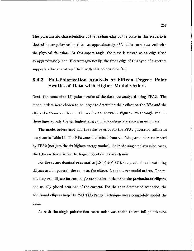
237
The polarimetric characteristics of the leading edge of the plate in this scenario is
that of linear polarization tilted at approximately 45'. This correlates well with
the physical situation. At this aspect angle, the plate is viewed as an edge tilted
at approximately 45' . Electromagnetically, the front edge of this type of structure
supports a linear scattered field with this polarization [49].
6.4.2 Full-Polarization Analysis of Fifteen Degree PolarSwaths of Data with Higher Model Orders
Next, the same nine 15' polar swaths of the data are analyzed using FPA2. The
model orders were chosen to be larger to determine their effect on the REs and the
ellipse locations and form. The results are shown in Figures 125 through 127. In
these figures, only the six highest energy pole locations are shown in each case.
The model orders used and the relative error for the FPA2 generated estimates
are given in Table 14. The REs were determined from all of the parameters estimated
by FPA2 (not just the six highest energy modes). As in the single polarization cases,
the REs are lower when the larger model orders are chosen.
For the corner dominated scenarios (150 < _< 750), the predominant scattering
ellipses are, in general, the same as the ellipses for the lower model orders. The re-
maining two ellipses for each angle are smaller in size than the predominant ellipses,
and usually placed near one of the corners. For the edge dominated scenarios, the
additional ellipses help the 2-D TLS-Prony Technique more completely model the
data.
As with the single polarization cases, noise was added to two full-polarization
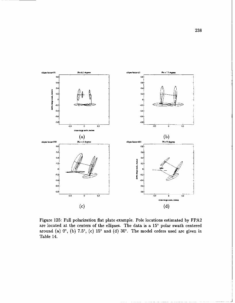
238
ellpsw f-tr=50 PM=0.0 dg ellip" factw-I 5 V. = 7.5 dSe
0.8 0.8-
0.6 0.6-
0.4 0.4
I0.2 0.2
00
-0.2 -0.2
-0.4 -0.4
-0.6 -0.6
-0.8 -0.8
-0.5 0 0.5 -0.5 0 0,5
w.-aMnge 8W., mAMs
(a) (b)elli fator=-.300 = 15 degm elhue fsctor=400 Phi=30 dtgm
0.8 0.8
0.6 0.6-
0.4- 0.4
0.2 I 0.2
0 ! 0
-0.2 -0.2
-0.4 -0.4
.0.6 -0.6
-0.8 -0.8
-0.5 0 0.5 -0.5 0 0.5
"aM m-ra ¢a
(c) (d)
Figure 125: Full polarization flat plate example. Pole locations estimated by FPA2are located at the centers of the ellipses. The data is a 150 polar swath centeredaround (a) 00, (b) 7.5', (c) 15° and (d) 30'. The model orders used are given inTable 14.
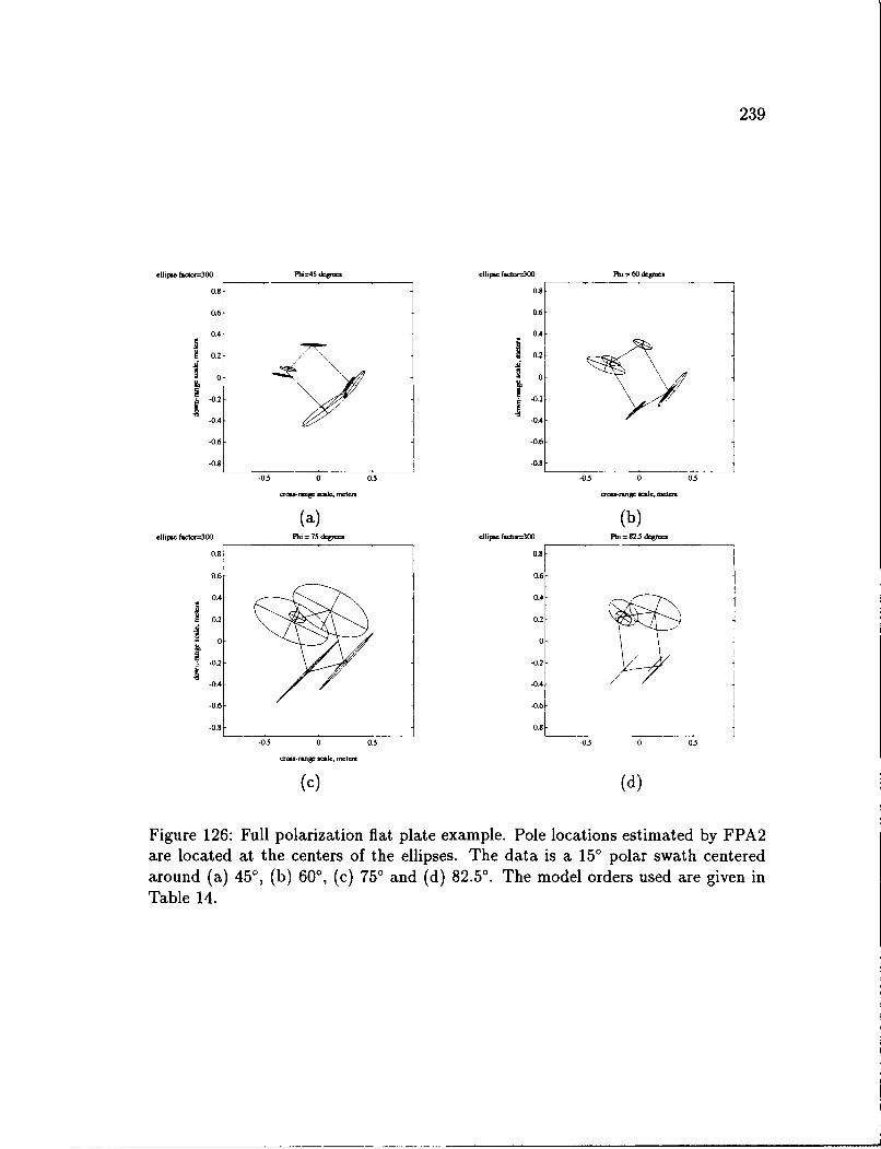
239
Mlip. tfdo.=300 PhI-45 &V-o .llirw f..o,-500 PhR, 60 dgi
0.8 0.8-
0.6- 0.6-
0.4- 0.4-
102 - 0
-0.4--0.4
-0.6 -0.6
-0.8 -.
-0.5 0 0.5 -0.5 0 0.
(a) (b).1hpw iedoeSOO Phi 75 dg-oe ibp. fon--=50 Pi 8235 &gre
0.8 0.8
0.6- 0.6-
0.'4 0.4-
1 0.2 0.2
0 0~:.0.2 -.
.0.4- -0.4
-0.6- -0.6
-0.8- -08
-0.5 0 0.5 _0 0 0.5
l-o mg! w, Wotof
(c) (d)
Figure 126: Full polarization flat plate example. Pole locations estimated by FPA2are located at the centers of the ellipses. The data is a 150 polar swath centeredaround (a) 450, (b) 600, (c) 750 and (d) 82.5'. The model orders used are given inTable 14.
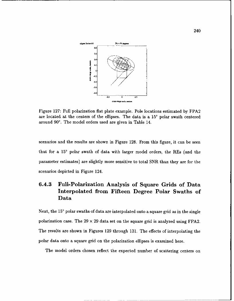
240
01hlpe f.1-50 Phi 90 >ec
0.8
0.6-
0.4S 0.2
-0.2
-0.4
-0.6
-0.8
-0.5 0 03
Figure 127: Full polarization flat plate example. Pole locations estimated by FPA2are located at the centers of the ellipses. The data is a 150 polar swath centeredaround 900. The model orders used are given in Table 14.
scenarios and the results are shown in Figure 128. From this figure, it can be seen
that for a 15' polar swath of data with larger model orders, the REs (and the
parameter estimates) are slightly more sensitive to total SNR than they are for the
scenarios depicted in Figure 124.
6.4.3 Full-Polarization Analysis of Square Grids of DataInterpolated from Fifteen Degree Polar Swaths ofData
Next, the 150 polar swaths of data are interpolated onto a square grid as in the single
polarization case. The 29 x 29 data set on the square grid is analyzed using FPA2.
The results are shown in Figures 129 through 131. The effects of interpolating the
polar data onto a square grid on the polarization ellipses is examined here.
The model orders chosen reflect the expected number of scattering centers on
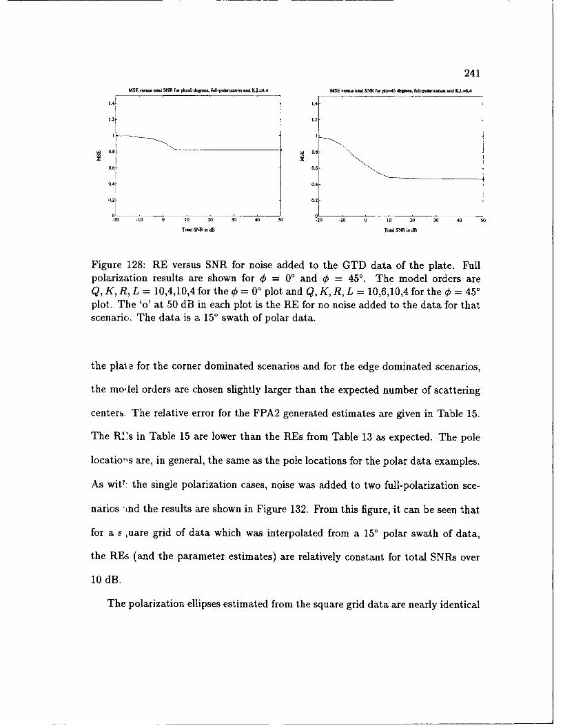
241
MSE v..t toW SNR fopb4 &W. Ifull-pol n on nd K.L=4,4 MSE voua toWta SNR fa pl =45 dogmes fxud-p.zuon. nDd KL=64
1.4 1.4-
L.2 -1.2
0.8- 0.8
0.6- 0.6
0.4 0.4
0.2 0.2
20 -10 0 0 20 30 40 50 -20 -10 0 10 20 30 40 0
Total SNR w dB Total SNR mdB
Figure 128: RE versus SNR for noise added to the GTD data of the plate. Fullpolarization results are shown for 0 = 0' and 0 = 45' . The model orders areQ, K, R, L = 10,4,10,4 for the € = 00 plot and Q, K, R, L = 10,6,10,4 for the € = 450plot. The 'o' at 50 dB in each plot is the RE for no noise added to the data for thatscenario. The data is a 150 swath of polar data.
the plat- for the corner dominated scenarios and for the edge dominated scenarios,
the model orders are chosen slightly larger than the expected number of scattering
centers. The relative error for the FPA2 generated estimates are given in Table 15.
The RL's in Table 15 are lower than the REs from Table 13 as expected. The pole
locatio-,s are, in general, the same as the pole locations for the polar data examples.
As wit': the single polarization cases, noise was added to two full-polarization sce-
narios "nd the results are shown in Figure 132. From this figure, it can be seen that
for a s ,uare grid of data which was interpolated from a 150 polar swath of data,
the REs (and the parameter estimates) are relatively constant for total SNRs over
10 dB.
The polarization ellipses estimated from the square grid data are nearly identical
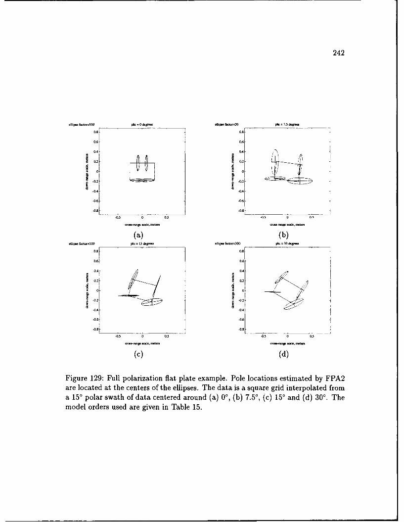
242
elipse fato=500 pl,. 0 &0-. ellips tudo-20 p.7.5 dW-
0.8- 0.8-
0.6- 0.6-
0.4- 0.4
1 02 0.2
.0.2l -0.2
-0.4 - -0.4
-0.6- -0.61
-08- -0.81
-0.5 0 0.0 -0.5 0 O
(a) (b)elipsec fact-=100 ph 15 ilgr- elipse fact=30 ph 30 dgrse,
0.8 -0.8
0.6- 0.6-
0.4- 0.4-
N 0.2 N 0.20i 0
-0.2 -0.24
-0.4 -0.4 J4
-0.6 -0.6
-0. 5- 0 0.5 -0.1 0.5 0 035
(c) (d)
Figure 129: Full polarization fiat plate example. Pole locations estimated by FPA2are located at the centers of the ellipses. The data is a square grid interpolated froma 150 polar swath of data centered around (a) 0', (b) 7.50, (c) 15' and (d) 30'. Themodel orders used are given in Table 15.
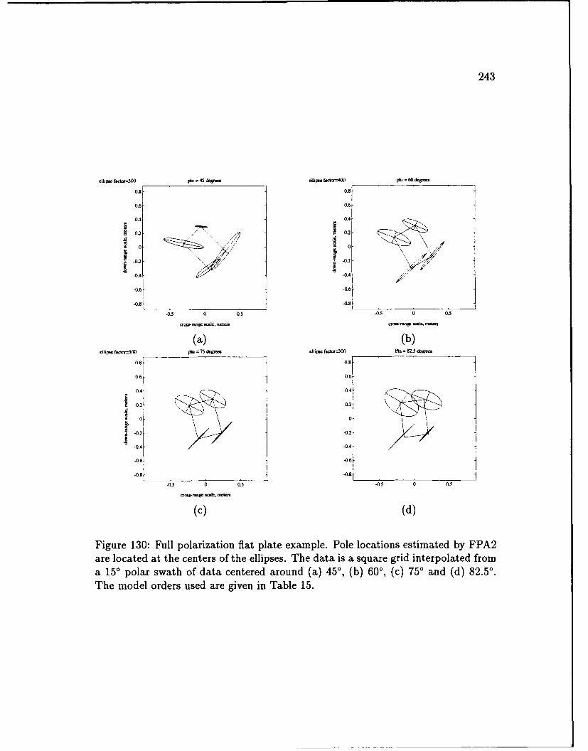
243
ellipse fd-=00 pt 5d ec lis f8whtr400 pt =60 dwp.
0.8- 0.8
0.6- 0.6-
0.4- 0.4-
0.2 10.2
-0.2- -0.2
-0.4 -0.4 h0
406-06
-0.5 0 05 5 0 0.5
(a) (b)elipse ttotor=3007h 75 &V-a ellipse facor300 Ph 82.5 dgcc
0.8- 0.8
0.6- 0.6
0.4- 0.4
0.2- 0.2
S -0.2- -0.2
-0.4- .. -
-0.6- -0.6-1
-0.8- ______________________
0. 0 05 .50 0.5
(c) (d)
Figure 130: Full polarization flat plate example. Pole locations estimated by FPA2are located at the centers of the ellipses. The data is a square grid interpolated froma 150 polar swath of data centered around (a) 450, (b) 600, (c) 75' and (d) 82.5'.The model orders used are given in Table 15.
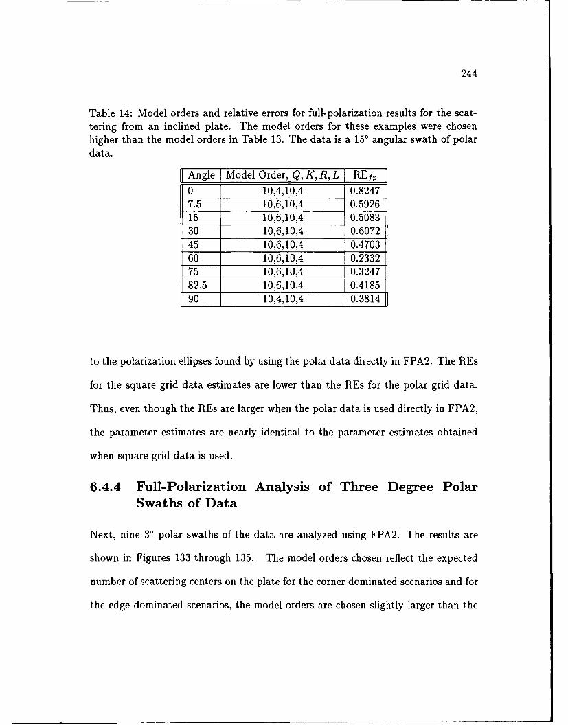
244
Table 14: Model orders and relative errors for full-polarization results for the scat-tering from an inclined plate. The model orders for these examples were chosenhigher than the model orders in Table 13. The data is a 150 angular swath of polardata.
I Angle ] Model Order, Q, K, R, L REfp
0 10,4,10,4 0.82477.5 10,6,10,4 0.592615 10,6,10,4 0.508330 10,6,10,4 0.607245 10,6,10,4 0.470360 10,6,10,4 0.233275 10,6,10,4 0.324782.5 10,6,10,4 0.418590 10,4,10,4 0.3814
to the polarization ellipses found by using the polar data directly in FPA2. The REs
for the square grid data estimates are lower than the REs for the polar grid data.
Thus, even though the REs are larger when the polar data is used directly in FPA2,
the parameter estimates are nearly identical to the parameter estimates obtained
when square grid data is used.
6.4.4 Full-Polarization Analysis of Three Degree PolarSwaths of Data
Next, nine 3' polar swaths of the data are analyzed using FPA2. The results are
shown in Figures 133 through 135. The model orders chosen reflect the expected
number of scattering centers on the plate for the corner dominated scenarios and for
the edge dominated scenarios, the model orders are chosen slightly larger than the
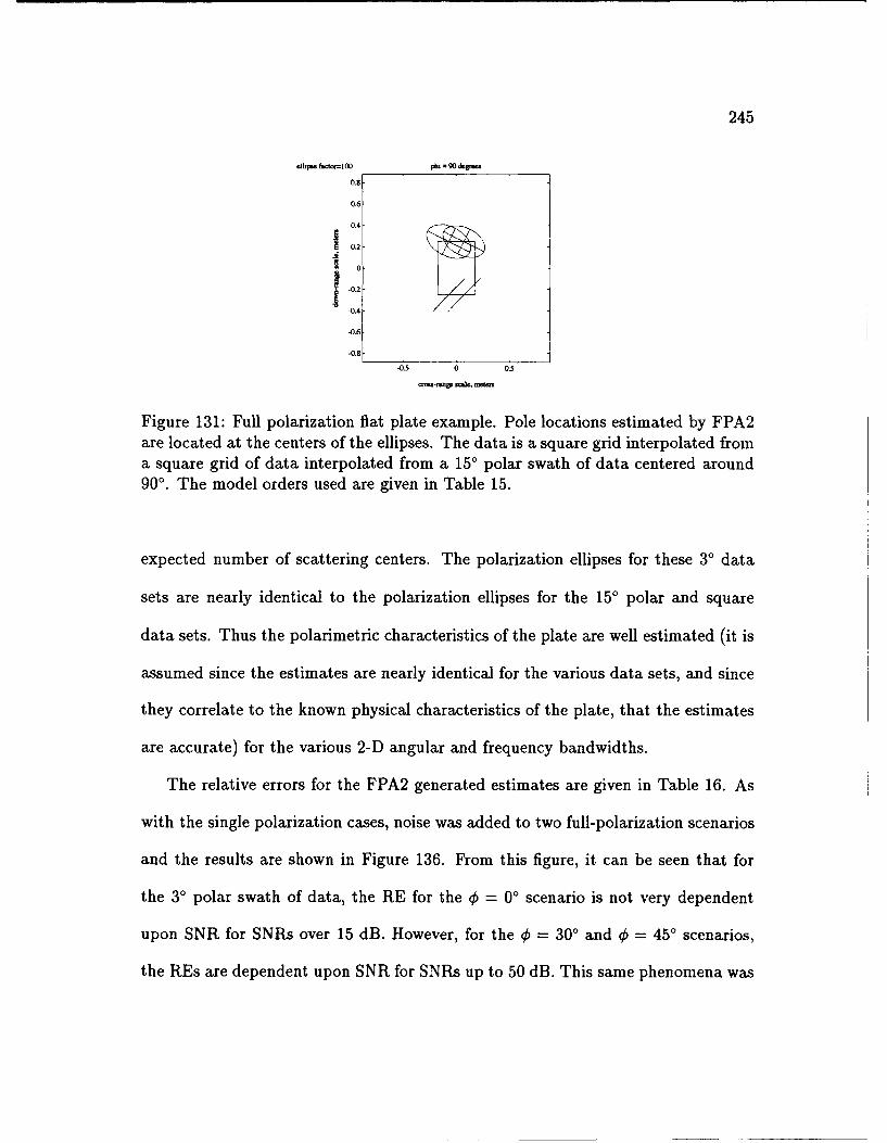
245
.Hip.. f.W-o0 ph, = 90 g
0.8
0.6
0.4
1 0.2
-0.2
-0.4
-0.6
-0.8-03 0 0.5
Figure 131: Full polarization flat plate example. Pole locations estimated by FPA2are located at the centers of the ellipses. The data is a square grid interpolated froma square grid of data interpolated from a 150 polar swath of data centered around900. The model orders used are given in Table 15.
expected number of scattering centers. The polarization ellipses for these 30 data
sets are nearly identical to the polarization ellipses for the 150 polar and square
data sets. Thus the polarimetric characteristics of the plate are well estimated (it is
assumed since the estimates are nearly identical for the various data sets, and since
they correlate to the known physical characteristics of the plate, that the estimates
are accurate) for the various 2-D angular and frequency bandwidths.
The relative errors for the FPA2 generated estimates are given in Table 16. As
with the single polarization cases, noise was added to two full-polarization scenarios
and the results are shown in Figure 136. From this figure, it can be seen that for
the 3' polar swath of data, the RE for the 0 = 00 scenario is not very dependent
upon SNR for SNRs over 15 dB. However, for the 0 = 30' and 0 = 450 scenarios,
the REs are dependent upon SNR for SNRs up to 50 dB. This same phenomena was
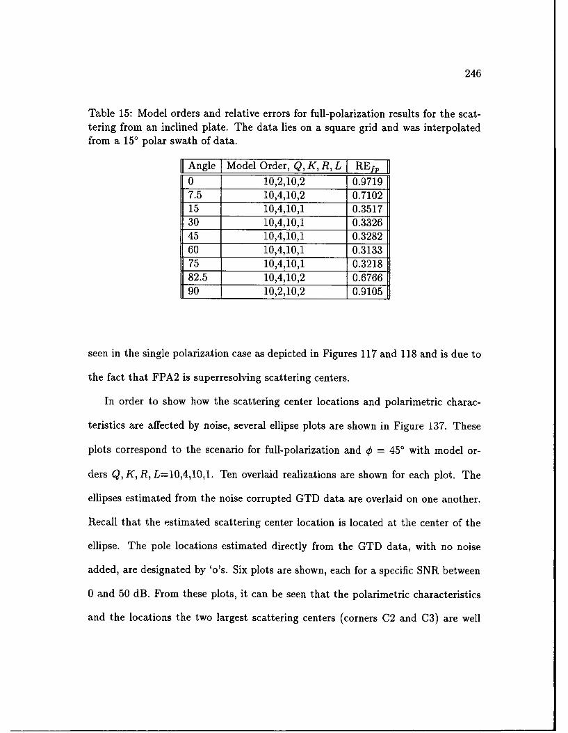
246
Table 15: Model orders and relative errors for full-polarization results for the scat-tering from an inclined plate. The data lies on a square grid and was interpolatedfrom a 150 polar swath of data.
]j Angle Model Order, Q, K, R, L REfp 1
0 10,2,10,2 0.97197.5 10,4,10,2 0.710215 10,4,10,1 0.351730 10,4,10,1 0.332645 10,4,10,1 0.328260 10,4,10,1 0.313375 10,4,10,1 0.321882.5 10,4,10,2 0.676690 10,2,10,2 0.9105
seen in the single polarization case as depicted in Figures 117 and 118 and is due to
the fact that FPA2 is superresolving scattering centers.
In order to show how the scattering center locations and polarimetric charac-
teristics are affected by noise, several ellipse plots are shown in Figure 137. These
plots correspond to the scenario for full-polarization and 0 = 450 with model or-
ders Q, K, R, L=10,4,10,1. Ten overlaid realizations are shown for each plot. The
ellipses estimated from the noise corrupted GTD data are overlaid on one another.
Recall that the estimated scattering center location is located at the center of the
ellipse. The pole locations estimated directly from the GTD data, with no noise
added, are designated by 'o's. Six plots are shown, each for a specific SNR between
0 and 50 dB. From these plots, it can be seen that the polarimetric characteristics
and the locations the two largest scattering centers (corners C2 and C3) are well
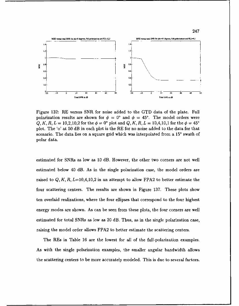
247
MSE veus toa SNR fmr phi=O dv fwi-poalrizValm and K 2,2 MSE numja toals NR fot pj=45 dav., ftdl-p and LL4I
1.4 1.4
1.2 1.2
ot 0.8 W 0.8
0.6 - 0.60.4- 0.4-
0.2 0.2
-20 -10 10 20 30 40 50
Total SNR m dB Total SNR -111
Figure 132: RE versus SNR for noise added to the GTD data of the plate. Fullpolarization results are shown for (k = 0° and 4 = 450. The model orders wereQ, K, R, L = 10,2,10,2 for the 4 = 0' plot and Q, K, R, L = 10,4,10,1 for the 4 = 450plot. The 'o' at 50 dB in each plot is the RE for no noise added to the data for thatscenario. The data lies on a square grid which was interpolated from a 150 swath ofpolar data.
estimated for SNRs as low as 10 dB. However, the other two corners are not well
estimated below 40 dB. As in the single polarization case, the model orders are
raised to Q, K, R, L=10,4,10,2 in an attempt to allow FPA2 to better estimate the
four scattering centers. The results are shown in Figure 137. These plots show
ten overlaid realizations, where the four ellipses that correspond to the four highest
energy modes are shown. As can be seen from these plots, the four corners are well
estimated for total SNRs as low as 20 dB. Thus, as in the single polarization case,
raising the model order allows FPA2 to better estimate the scattering centers.
The REs in Table 16 are the lowest for all of the full-polarization examples.
As with the single polarization examples, the smaller angular bandwidth allows
the scattering centers to be more accurately modeled. This is due to several factors.
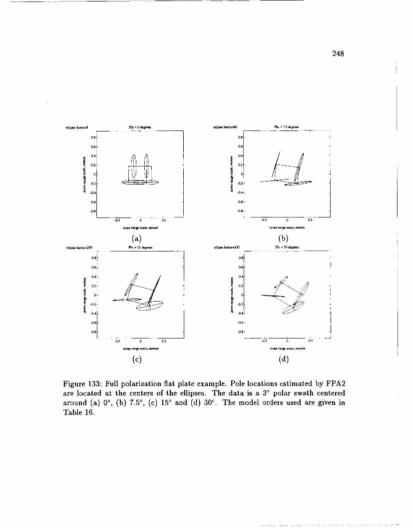
248
Sllis fNctor"-8 M= 0 ddg. ellipic fa t" o80 PIh : 7.5 dkgrem
0.8 0.8
0.6 0.6
0.2- 0 .204
0 .
.-8 -0.4
-0.6 -0.6
-0.8 -0.8
-0.5 0 0.5 -0.5 0 0.5
teass-ma ste, meters ama-rale, met
(a) (b)ellipse facto--200 Phi: 15 degr-; ellp.e fcto--300 Ph. 30 dgcs
0.8 0.8-
0.6 0.6
0.4-/ 0.4
0.2- 0.2
0-- 0
-0.6 -0.6-0.8 -0.8
-0.5 0 0.5 -05 0 (a5
~rcnl- ratrll satle. mneters ce"tlm.- rstt s = ale. metcersl
(c) (d)
Figure 133: Full polarization flat plate example. Pole locations estimated by FPA2are located at the centers of the ellipses. The data is a 30 polar swath centeredaround (a) 0', (b) 7.5', (c) 150 and (d) 300. The model orders used are given inTable 16.
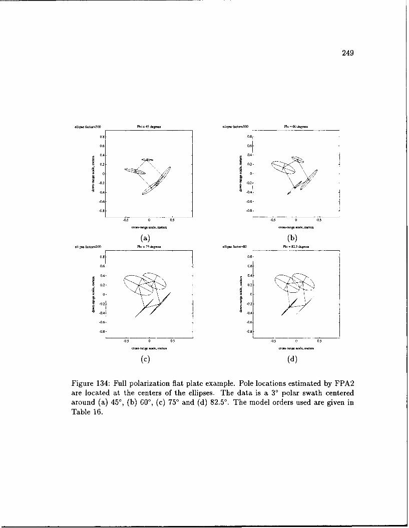
249
ellipse facto=--300 Pt = 45 dgo- cllip" fi-ctor-300 P1 = 60 dgr-.
0.8 0.8
0.6 0.6
0.4 0.4
-0.2 -0.2
-0.4 -0.4 #
-0.6 -0.6
-0.8 -0.8
-0.5 0 0.5 -0.5 0 0.5
nase ". sle, ee. -rmn, sale, oser
(a) (b)elhpe factr=-20
0 Mt, = 75 dige. elliple flto-80 Pi = 82.5 dq-re.
0.8 0.8
0.6 0.6
0.4 . 0.4
0.2 0.2
0- 0
-0.2 -0.2
-0.4 -0.4
-0.6 -0.6
-0.8 -0.8
0.5 0 0.5 -0.5 0 0.5
ces-rme scale, moron aa*-.rOWg sale-. tet ero
(c) (d)
Figure 134: Full polarization flat plate example. Pole locations estimated by FPA2are located at the centers of the ellipses. The data is a 30 polar swath centeredaround (a) 450, (b) 6O0 , (c) 750 and (d) 82.50. The model orders used are given inTable 16.
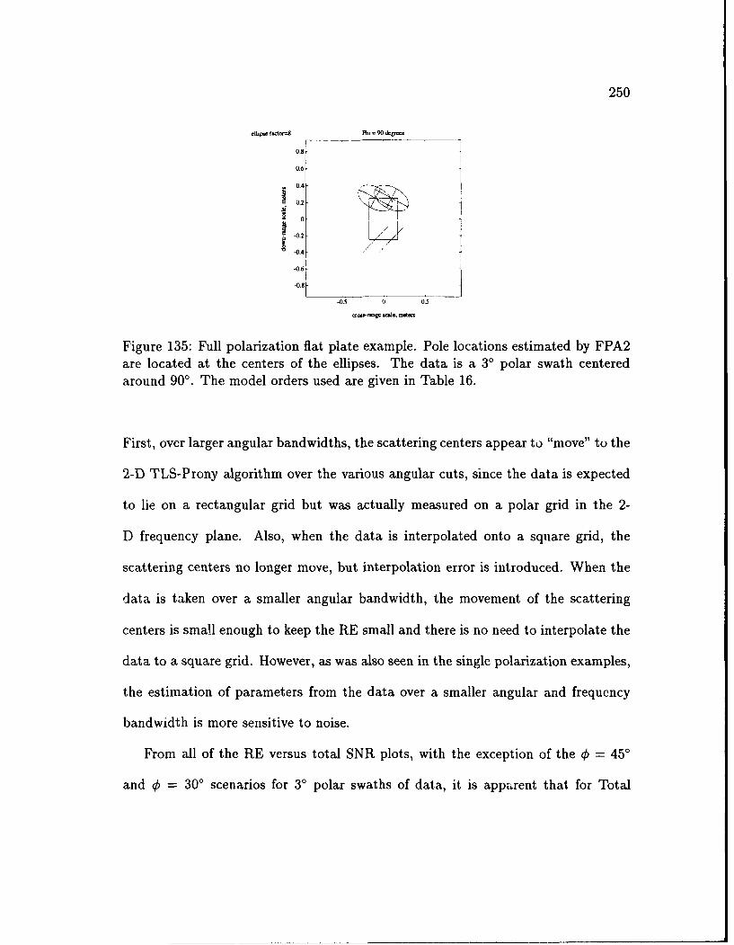
250
.llpt fuf --8 Ph. 90 & 9 -
0.8
0.6-
1 0.44
0
-0.2
-0.4
-0.6
-0.8
-05 0 0.5
Figure 135: Full polarization flat plate example. Pole locations estimated by FPA2are located at the centers of the ellipses. The data is a 3' polar swath centeredaround 900. The model orders used are given in Table 16.
First, over larger angular bandwidths, the scattering centers appear to "move" to the
2-D TLS-Prony algorithm over the various angular cuts, since the data is expected
to lie on a rectangular grid but was actually measured on a polar grid in the 2-
D frequency plane. Also, when the data is interpolated onto a square grid, the
scattering centers no longer move, but interpolation error is introduced. When the
data is taken over a smaller angular bandwidth, the movement of the scattering
centers is small enough to keep the RE small and there is no need to interpolate the
data to a square grid. However, as was also seen in the single polarization examples,
the estimation of parameters from the data over a smaller angular and frequency
bandwidth is more sensitive to noise.
From all of the RE versus total SNR plots, with the exception of the 4 = 450
and 4 = 30' scenarios for 3' polar swaths of data, it is apparent that for Total
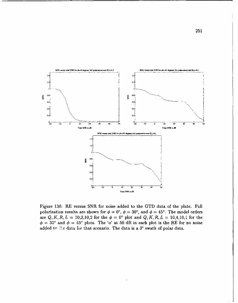
251
MSE vt tot.] SNR fm pu=( e &rs, ful-polwuzmb c t K , 2-,2 MSE v .s total SNR fo phi=45 dt em fu-podnxsbw and KL=4 1
1.4- 1.4
1.2- 1.2
t 0.8 t 0.8
0.6 0.6-
0.4 0.4-
0.2 02-
0 0-20 -10 0 10 20 30 40 50 -20 -10 0 10 20 30 40 50
Total SNR idB Tot.] SNR m dB
MSE vel tot l SNR fm it=30 &gms, full-polanzaton d KL.1-,
1.4k 1
1.2 -.
0.6 10.4
02
0-20 -10 0 10 20 30 40 S0
Toal SNR m dB
Figure 136: RE versus SNR for noise added to the GTD data of the plate. Fullpolarization results are shown for ' = °, 0 = 30', and 4 = 45' . The model ordersare Q, K, R, L = 10,2,10,2 for the € = 00 plot and Q, K, R, L = 10,4,10,1 for the0 = 30 ' and q = 450 plots. The 'o' at 50 dB in each plot is the RE for no noiseadded to 1.e data for that scenario. The data is a 30 swath of polar data.
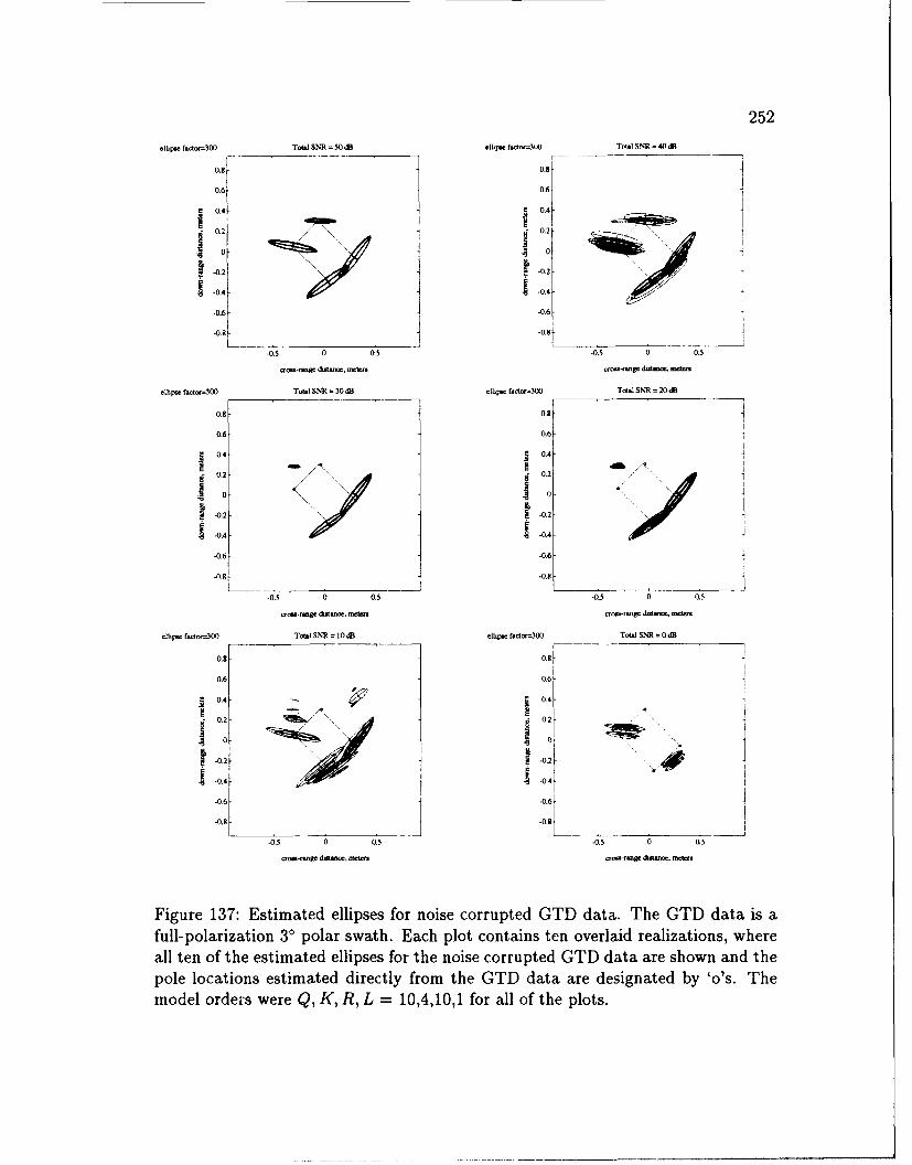
252
.ilhp. at.,r=300 Toal SNR 50 .B IIh.c foo,1M10 To.] SNR = 40 dosg
0.0.8-
0.6 0.6
j0.4
_ 0.4
0 o2 -o0.2--0-
-0.2- -. 2-
-0.4-- -0.4-
-0.6 -0.6-
-0.98 -0.8
-0.5 0 0.5 -0.5 0 0.5
.lhp fato-300 Tot.I SNR = 30dB tl0p fao-300 Tol.W SNR = 20 dB
0.8 0.8 !
0.6- 0.6,
0.4-j 0.4
Aft0.2 0.2
0 0
-0.2 0.2
-0.6 -0.6
-0.6 -0.8
-0.5 0 0.5 -05 0 0.5
.mc-pg dim-= rrWx a -mage dwtano met
ell!p fact-=300 Toi SNR = 10,B ohI ftsor-300 To.1 SNR = OdB
0.8 O
0.6 0.2
0.2 -0.2
0.4 .04 4
-06 -0-6
-0.9 -0.8
-0.5 0 0a5 -0.5 0 05
o. -p da. wtmm oa-~ge dst . mwft
Figure 137: Estimated ellipses for noise corrupted GTD data. The GTD data is afull-polarization 30 polar swath. Each plot contains ten overlaid realizations, whereall ten of the estimated ellipses for the noise corrupted GTD data are shown and thepole locations estimated directly from the GTD data are designated by 'o's. Themodel orders were Q, K, R, L = 10,4,10,1 for all of the plots.
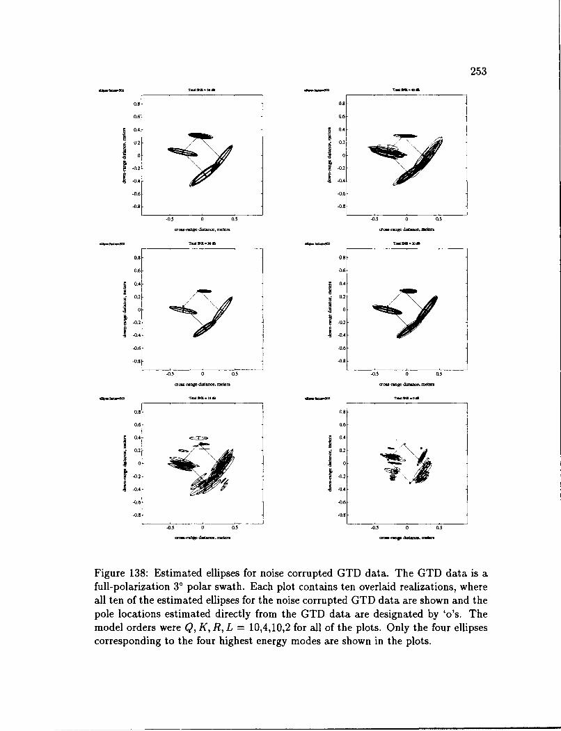
253
0.8 0.8
0.6 0.6
0
S-0.2 - -0.2
-06- -0.
-0.4 -0.8
-0.5 0 0.5 -0.5 0 0.5
m~s-rnge ditne, metr a-nWag d mean
0.8 0.8
0.6 0.6
0.2 7 0.2
00
-02 -0.
-0.6 -0.6
-0.8 -0.8
-0.5 0 0.5 -0.5 0 0.5
aano3 W.~t.a. So
0.8 0.8
0.6 0.6
0.4- 0.4-
.2 02
0 10
-0.2 02
I -0.4 I -04
-0.6 -0.6
-0.8 -0.8
-0.5 0 0.5 .0.5 0 i.5
cr--Mg. dw-n, -& am-r'WW &d.. a-
Figure 138: Estimated ellipses for noise corrupted GTD data. The GTD data is afull-polarization 30 polar swath. Each plot contains ten overlaid realizations, whereall ten of the estimated ellipses for the noise corrupted GTD data are shown and thepole locations estimated directly from the GTD data are designated by ''s. Themodel orders were Q, K, R, L = 10,4,10,2 for all of the plots. Only the four ellipsescorresponding to the four highest energy modes are shown in the plots.
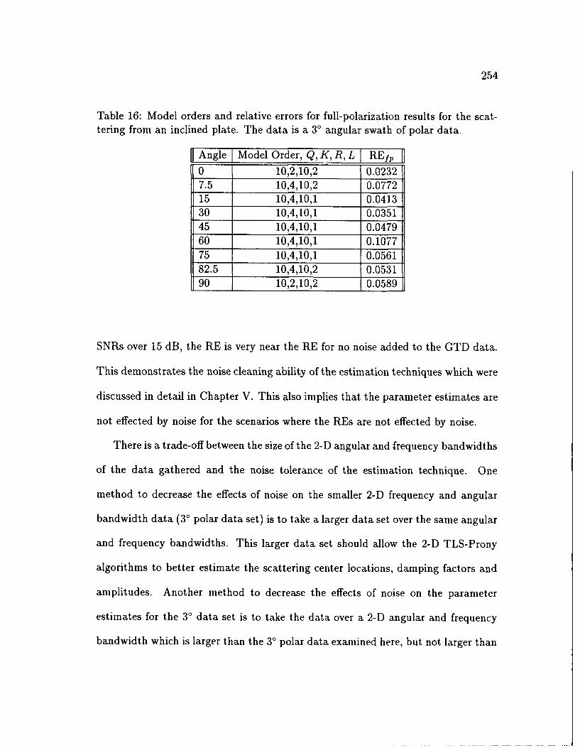
254
Table 16: Model orders and relative errors for full-polarization results for the scat-tering from an inclined plate. The data is a 3' angular swath of polar data.
Angle I Model Order, Q, K, R,L RE1f ]p0 10,2,10,2 0.02327.5 10,4,10,2 0.077215 10,4,10,1 0.041330 10,4,10,1 0.035145 10,4,10,1 0.047960 10,4,10,1 0.1077
75 10,4,10,1 0.056182.5 10,4,10,2 0.053190 10,2,10,2 0.0589
SNRs over 15 dB, the RE is very near the RE for no noise added to the GTD data.
This demonstrates the noise cleaning ability of the estimation techniques which were
discussed in detail in Chapter V. This also implies that the parameter estimates are
not effected by noise for the scenarios where the REs are not effected by noise.
There is a trade-off between the size of the 2-D angular and frequency bandwidths
of the data gathered and the noise tolerance of the estimation technique. One
method to decrease the effects of noise on the smaller 2-D frequency and angular
bandwidth data (30 polar data set) is to take a larger data set over the same angular
and frequency bandwidths. This larger data set should allow the 2-D TLS-Prony
algorithms to better estimate the scattering center locations, damping factors and
amplitudes. Another method to decrease the effects of noise on the parameter
estimates for the 30 data set is to take the data over a 2-D angular and frequency
bandwidth which is larger than the 30 polar data examined here, but not larger than

255
the 150 data set (thus, somewhere around 60 may be appropriate).
The results for the 150 polar swaths of data (both on the original polar grid and
the square grid) had REs which can be considered high, but they still estimated the
scattering center locations and damping factors well, as can be seen by comparing
the results for these cases with the results for the 30 polar swaths of data. It is not
necessarily true that if a given model models the data with a larger RE, that the
parameter estimates are not representative of the modes which exist in the data.
For the 150 polar swaths of data, it is assumed that the parameter estimates are
accurate, since they match the parameter estimates for the 30 polar swaths of data,
with no noise added to the data. The 30 polar swaths of data, with no noise added
to the data, are considered accurate since the REs associated with these data sets
are relatively low.
6.5 Analysis of Individual Scattering Centers on Plate
Recall from Chapter III that the response of a corner as a function of frequency is1
and as a function of angle is a constant (for non-grazing situations). In Chapter III,
the ability of a damped exponential to model the frequency behavior of a corner
was demonstrated. Here, the frequency and angle responses of the estimates for the
individual corners on the plate are compared to the I and constant behaviors of
a corner. Consider the single polarization plate simulation for hh-polarization and
€ = 45' . Two data sets are examined, the square grid of data interpolated from the
150 swath of polar data, and the 30 swath of polar data. For both data sets, eight
plots are shown over two figures.
256
The GTD code described in [49] has the capability to predict the scattering due
to an individual corner on the plate. This capability is used here. The 2-D TLS-
Prony Technique is used to estimate the parameters from a data set which contains
the scattering response of a single corner on the plate. The model orders are set
at Q, K, R, L =10,1,10,1 for the scenarios where the data contains the scattering
response for a single corner on the plate. For the 2-D Prony Model in Equation 5.2,
recall that the x-poles correspond to the frequency portion of the 2-D frequency
domain data while the y-poles correspond to the angle portion of 2-D frequency
domain data.
For each data set, the first four plots contain frequency response data, one plot
for each corner of the plate. Shown are the frequency responses at 450 as taken
from the data (solid line) and as estimated by the model. Two model estimates are
show in each plot; the first (dashed line) corresponds to the estimates from the data
set generated for only one corner of the plate while the second (dash-dotted line)
corresponds to the estimates from the complete data set for the plate. Also show in
each plot is the model assumed 1 behavior for the corner (dotted line, this plot is
difficult to see since it nearly overlaps the solid line).
The second four plots for each data set contain angular response data, one for
each corner of the plate. As with the frequency response plots, shown are the angular
responses at 45' as taken from the data (solid line) and as estimated by the model.
Two model estimates are show in each plot, the first (dashed line) corresponds to
the estimates from the data set generated for only one corner of the plate while the
257
second (dash-dotted line) corresponds to the estimates from the complete data set
for the plate. The model assumed constant behavior of the corner is not shown in
the angular plots.
From the results show in Figures 139 through 142, it is observed that the damped
exponential model is appropriate for the scattering from the corners of the plate
around q = 450, as was also concluded in Chapter III. Several full-polarization
scenarios were run (but not shown here) and the results are similar to the results
shown for the single-polarization case. In the figures corresponding to the angular
dependencies of the scattering centers, it is seen that the data shown is not con-
stant as a function of angle, but a smooth function which is close to a constant. A
more appropriate model for the angular behavior of a corner (in non-grazing situa-
tions) might be a damped exponential, which, of course, is what is used in the 2-D
TLS-Prony Technique. A constant was chosen in Table 1 since it was the simplest
model which was close to the actual scattering behavior of a corner in non-grazing
situations.
6.6 Summary
In this chapter several radar target modeling examples, involving simulated radar
data, were discussed. The scattering from an inclined thin metal plate was gener-
ated using the GTD. This data was then used by both the single-polarization and
the full-polarization 2-D TLS Prony Techniques to estimate he locations, damp-
ing factors and polarimetric characteristics of the scattering centers on the plate.
Issues involving 2-D angular and frequency bandwidths, model order selection, ef-
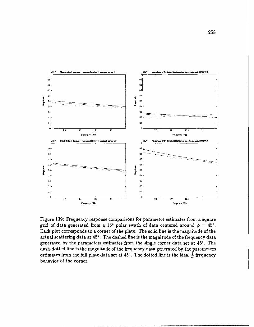
258
.104
MWtuk of r uq"cy rq- f. pht=45
dg. . - CI x 10-
Mgnfl of fr eqwoy z mc fm =45 dgre. ox C2I I
0.9 0.9
0.8 0.8
0.7 0.7
0.6 0.6
as .- 0.5
0.4 0.4
0.3 0.3----------- ---------
0.2 - 0.2 -- ----.. .. ........- -- --- ---
00L
9.5 10 10.5 11 9.5 10 10.5 11
Fnq-.cy, 0Hx F-q y,
xl04
M. ito& of frq.,y .p- fo phi=45 d&gs. o Con C3 lO. Magnitu&i of froquaoy rWme fa phi4=5 dW , r C4
III
0.90.0.9
0.6 0.6
0.5 0.5
0.4 0.4
0.3 0.3
0.2 0.2
0.1 0.1L
0 09.5 10 10.5 II 9.5 10 10.5 11
Fmq-~cy, ~h. F-,.cab
Figure 139: Frequeny response comparisons for parameter estimates from a squaregrid of data generated from a 150 polar swath of data centered around 0 = 45'Each plot corresponds to a corner of the plate. The solid line is the magnitude of theactual scattering data at 45'. The dashed line is the magnitude of the frequency datagenerated by the parameters estimates from the single corner data set at 45'. Thedash-dotted line is the magnitude of the frequency data generated by the parametersestimates from the full plate data set at 450. The dotted line is the ideal I frequencybehavior of the corner.
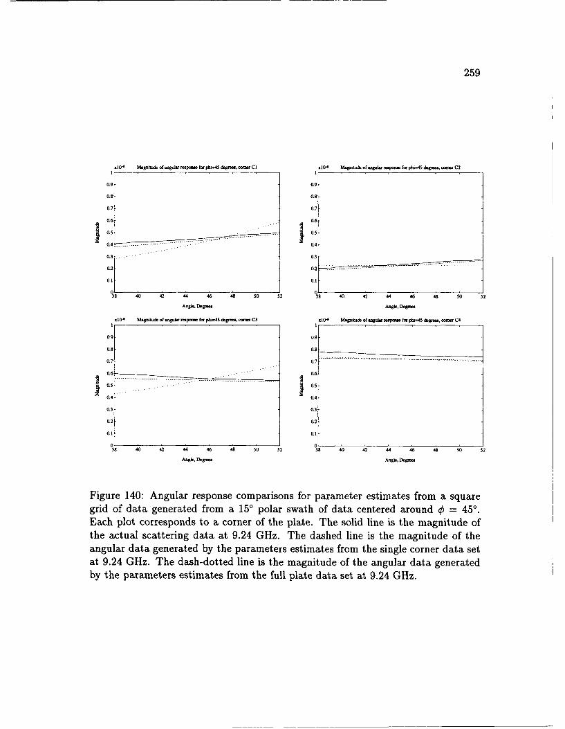
259
,i104 Magnitude of angular -rpovue, for phi=45 degrees CI X1O' Maguitude of angular novae for piu-45 deie or. ei C2
0L9 -089
0.7- 0.7-
0.6- 0.6-
0.530.4 .. .. - - -_ -- -- - -- _ - O
0.3.- 0.3-
0 .220
20.1 0.1
j ~0:38 40 42 44 46 48 5 5 8 40 42 44 46 48 so 52
AngI., Degnees Angle. Drg ~x1O' Ma~gnitude of angular -pone for plu=45 dgneea. core C3 olO6 Magnitude of angular resos for plu=45 dqpfts C4
0.9 0.9-
0.8 0.8-
0.6 . . .. 0.6
-- -----------. . . . . . . . . . . . .
0.4 0.4
0.3 -0.3
0.2 0.
0.1 0.1
38 40 42 44 46 49 50 52 38 40 42 44 46 48 so 52
An&l, Orgoc Anogle, Derg-
Figure 140: Angular response comparisons for parameter estimates from a squaregrid of data generated from a 150 polar swath of data centered around 4)=450.Each plot corresponds to a corner of the plate. The solid line is the magnitude ofthe actual scattering data at 9.24 GHz. The dashed line is the magnitude of theangular data generated by the parameters estimates from the single corner data setat 9.24 GHz. The dash-dotted line is the magnitude of the angular data generatedby the parameters estimates from the full plate data set at 9.24 GHz.
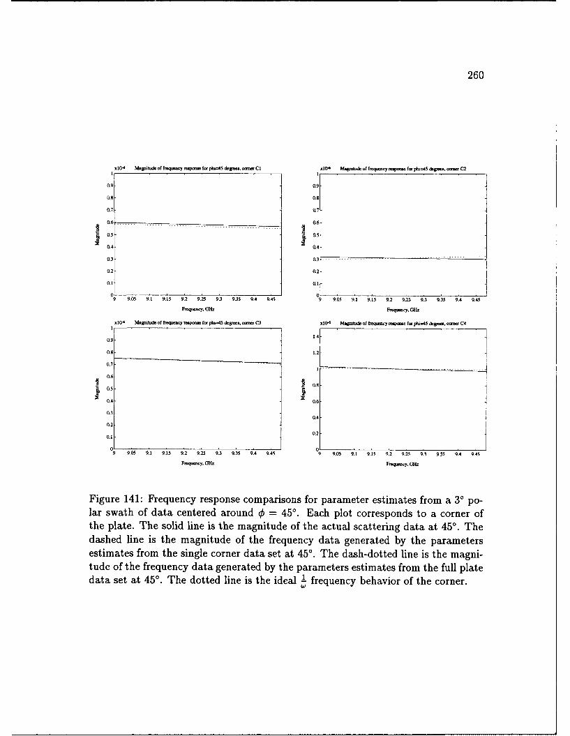
260
xlO- Magmtud of fhq.y .po f., pho=45 dsgbe , CI xlO4 MJpitd.l of fruq"ny rmoq- fo phi=45 k , o,-n, C2
0.9 0.9
0.7 0.7
0.6 0.6-
0.5 -0.5
0.4- 0.4
0.3 0.3
0.2 0.2-
0.1 0.1
9.05 9.1 9.15 9.2 9.25 9.3 9.35 9.4 9.45 9 9.05 9.1 9.15 9.2 9.25 9.3 9.35 9.4 9.45
Fequecy. 61k Frqey, GH
x104 I4.grtuk of freqecy Tspons for pf =45 'gzos, d cae C3 x10. Magmtude of fteqrocy rnooo fo phi=45 -greta, C4
140.9
1
0.8 1.2
0.7
I
0.6 t 0.90.5 *0.4 0.6
0.30.4
0.20.1
0.2
9 9.05 9.1 9.15 9.2 9.25 9.3 9.35 9.4 9.45 9 9.05 9.1 9.15 9.2 9.25 9.3 9.35 9.4 9.45
Freqe.ooy. G- Fmqocy, 61k
Figure 141: Frequency response comparisons for parameter estimates from a 30 po-lar swath of data centered around 0 = 45' . Each plot corresponds to a corner ofthe plate. The solid line is the magnitude of the actual scattering data at 45. Thedashed line is the magnitude of the frequency data generated by the parametersestimates from the single corner data set at 45'. The dash-dotted line is the magni-tude of the frequency data generated by the parameters estimates from the full platedata set at 45'. The dotted line is the ideal _! frequency behavior of the corner.1 )
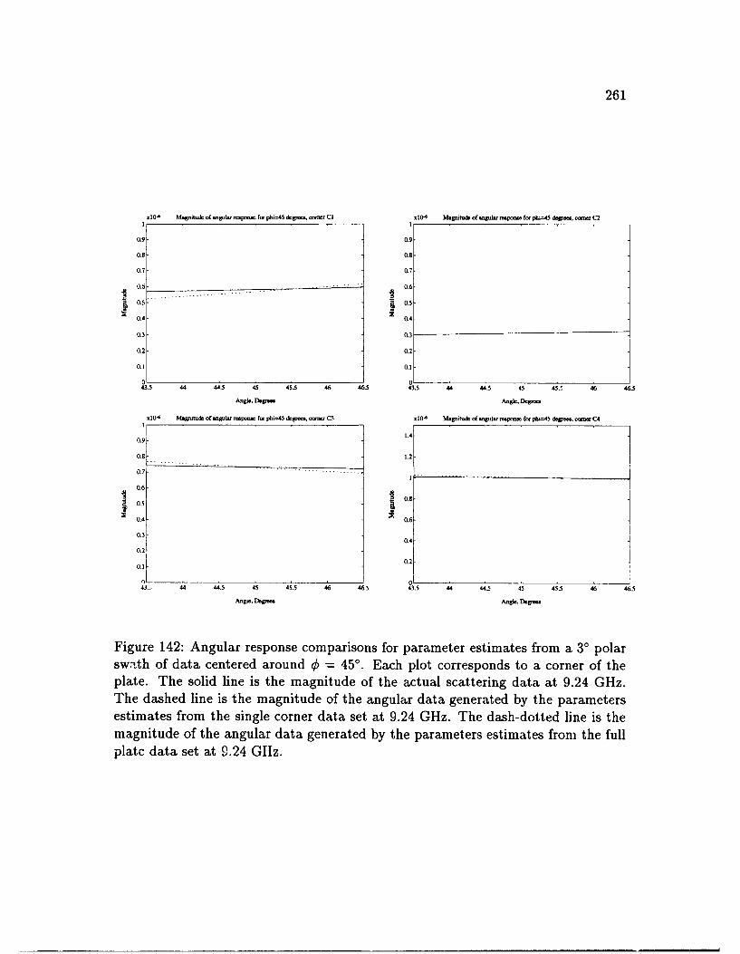
261
.lO Magiwd& of -go.W -p- f. pui=45 4&F-, o o CI x104
Mzgmhxk of wkgulr .Ipo fo, phoAS depoo C2I ,,
0.9 0.9
0.8 0.8-
0.7 0.7-
0.6 0.6-
0.5 0.5-
0.4 0.4-
0.3 -03
02 0.2-
0.1 0.1l
o o,43.5 44 44.5 45 45.5 46 46.5 43.5 44 44.5 45 45.' 46 46.5
Angle, Mg- Angl., D~gro.
X104 Mgnitde of .ngolso mxo fo phl-45 dgr-. o 3 o lo. Magoite of .gulor raspo fro45 degre.o ftmm - C4
"9 1.4-
0.9
0.8 1.2-
0.7 - - - -- -
0.6-
0.80.5
0.4 j 0.60.3 -!
0.4
0.2-
0.1 _ 0.2
n0143., 44 44.5 45 45.5 46 46.5 43.5 44.5 45 45.5 46 4.5
Ang., 1.W An& , lD.V-
Figure 142: Angular response comparisons for parameter estimates from a 3' polarswath of data centered around 0 = 45'. Each plot corresponds to a corner of theplate. The solid line is the magnitude of the actual scattering data at 9.24 GHz.The dashed line is the magnitude of the angular data generated by the parametersestimates from the single corner data set at 9.24 GHz. The dash-dotted line is themagnitude of the angular data generated by the parameters estimates from the fullplatc data set at 9.24 GIz.

262
fects of noise on parameter estimates, and the form (polar grid or square grid) of
the data set on the 2-D frequency plane were addressed. Also, the validity of the
damped exponential to model the scattering from the canonical scattering centers
was addressed.

CHAPTER VII
Summary and Conclusions
7.1 Summary of Work and Conclusions
This focus of this work has been to develop signal processing algorithms and models
for the scattering from radar targets. The models, which are summarized in Table 1,
are based upon the high-frequency electromagnetic scattering characteristics of the
canonical scattering centers analyzed. The algorithms developed can be used to
reduce the raw radar data of a complicated radar target to a set of estimated de-
scriptive parameters which can be used by a classification algorithm to identify the
target. As stated before, a basic assumption of this work is that the scattering from
radar targets can be comprised as the sum of the scattering from a finite number of
canonical scattering centers in the high-frequency case. This is a valid assumption if
the scattering centers are electrically isolated. This is also a reasonable assumption
even if two scattering centers are electrically close, since their combined response
can be treated as the response from a new type of canonical scattering center. Re-
call that the high-frequency case implies that the overall target size is at least one
wavelength.
The electromagnetic modeling of the canonical scattering centers used exact and
263
264
approximate methods of scattering prediction. Exact methods were used where
possible. The sphere for all aspect angles has an exact scattering solution for plane
wave incidence. The right-circular cylinder also has an exact scattering solution, but
only for limited aspect angles. The remainder of the canonical scattering centers
analyzed do not have exact scattering solutions, and approximate techniques such
as the Method of Moments (MM) and the Geometrical Theory of Diffraction (GTD)
were used to estimate their scattering characteristics. The MM and the GTD were
both used to predict the scattering from canonical scattering centers such as the
corner, edge, flat plate, dihedral, and trihedral. Once the scattering characteristics
of all of the canonical scattering centers were investigated, models were developed
and are summarized in Table 1. These models characterize the scattering from the
canonical scattering centers as functions of frequency and angle. These exact mod-
els are not contained in the 2-D damped exponential Prony model in Equation 5.2,
but the damped exponential model can accurately approximate most of the electro-
magnetically based models in Table 1. All of the frequency models and one of the
angular models are well approximated by damped exponentials. Two of the angular
models, however, are not well modeled using damped exponentials, as discussed in
Chapter III.
The reason that a damped exponential model was chosen as the model for the
2-D TLS-Prony Technique over the electromagnetically based models is that the
estimation algorithm developed for the 2-D TLS-Prony Technique required a damped
exponential model. Recall that the 2-D TLS-Prony Technique is an extension of
265
the 1-D TLS-Prony Technique developed in [29]. It may be possible to develop a
2-D estimation algorithm based on a model which directly uses the electromagnetic
models, but that is beyond the scope of this work. This type of estimation algorithm
has been developed in 1-D by Carribre and Moses [61].
It must also be noted that even though the damped exponential does not model
all of the scattering centers well, it is still an improvement in the modeling of radar
scattering. Much of the previous work in RTI assumed a point scatterer model for
the scattering from all types of canonical scattering centers [34], [35], [39]. The
extension to a 2-D damped exponential model is an improvement over the point
scatterer model.
The 2-D TLS-Prony Technique is not limited to the analysis of radar signals.
As demonstrated in Chapter V, the technique is capable of solving the general 2-D
frequency estimation problem. This technique can be applied to other areas such as
tomography, sonar, radio astronomy, and medical imaging to name a few. The use
of damped exponentials allows the poles in transform domain spectra (range-domain
in the radar problem) to have a dispersion. This is useful in modeling radar targets.
The execution time of this algorithm can be optimized since several of the steps
require a number of independent calculations which can be done in parallel.
The statistics of the 2-D TLS-Prony Technique algorithms are estimated and
compared to their respective Cram6r-Rao Bounds (CRBs) in Chapter V for some
undamped and damped exponentials in noise examples utilizing a number of Monte-
Carlo simulations. The x and y-pole estimates had different statistics, the x-pole
266
estimates being more accurate than the y-pole estimates, when Algorithm One and
FPA1 were used since the y-pole estimates were based on the x-amplitude coefficients
as the input data. Thus, a propagation of error caused the y-poles estimates to
have variances which were farther away from their respective CRBs than the x-pole
variances were away from their respective CRBs. This difference in estimates was
removed in Algorithm Two and FPA2 by utilizing the original algorithms twice.
First, the x-poles are estimated and then the y-poles are estimated. Then the
y-poles are estimated first followed by the x-poles. These two sets of pole pairs
are combined and the more accurate estimates from each set are retained. This
method achieves y-pole estimates which are as accurate as the x-poles. Asymptotic
expressions (asymptotic in SNR) for the actual statistics of the 1-D TLS-Prony
estimation algorithm have been developed by Ying [62]. In future work, these results
can be extended to achieve asymptotic expressions for the variance of the pole
locations and amplitude coefficients for the 2-D TLS-Prony Technique.
The simulations described in Chapter VI demonstrate some of the capabilities
and limitations of the 2-D TLS-Prony Technique. The ability of the 2-D TLS-Prony
Technique to determine the scattering center locations for various angular and fre-
quency bandwidths is well demonstrated. Comparing the single-polarization results
and the full-polarization results, it is apparent that the full-polarization ellipses give
an excellent representation of the polarimetric characteristics of each scattering cen-
ter on a target. There is a trade-off involving the angular and frequency bandwidths
on the 2-D frequency plane when the polar data is directly used by the algorithms.
267
For larger angular and frequency bandwidths (150 for this work), the effects of noise
on the parameter estimates and the relative error (RE) are insignificant for SNRs
over 15 dB; however, the RE is relatively high. For smaller angular and frequency
bandwidths (30 for this work), the effects of noise are more severe than they are
for the larger bandwidths, but the RE between the model and the original data is
relatively small for high SNRs when compared to the larger angular and frequency
bandwidths. The effects of noise on the parameter estimates for the smaller angular
and frequency bandwidths are demonstrated in the scatter plots shown for the 30
polar data cases. For low SNR, the parameter estimates are degraded and this is
reflected in the larger RE. Thus, for low SNR and smaller angular bandwidths it
is appropriate to use a larger model order as discussed and demonstrated in Chap-
ter VI.
The superresolution capabilities of the 2-D TLS-Prony Technique is demon-
strated in two sets of simulations. First, the simulations in Chapter V involve
sinusoids in noise which are only 0.4 Fourier Bins apart. The 2-D TLS-Prony Tech-
nique easily resolves the sinusoids for SNRs as low as 10 dB. Second, the flat plate
examples in Chapter VI for the 30 polar swaths of data also demonstrate superres-
olution capabilities. The contour images of the plate generated using the 2-D IFI7T
show peaks in the range domain which are not located on the corners of tl.e plate,
but the estimated scattering center locations do lie almost exactly (much closer than
the peaks in the contour image) on the corners of the plate, as thcy should.
For the data which was interpolated onto a square grid, thu REs were lower than
268
the REs for the equivalent data on a polar grid, but the estimated pole locations
were, in general, the same for either polar or square data over the same 2-D band-
widths. The REs may be reduced for the square grid data by developing a more
appropriate interpolation method. The one used is a linear function to estimate the
data values on the square grid from the surrounding polar values. An interpolation
algorithm which takes the nature of the data into account may be more appropriate.
The analysis of the single scattering centers at the end of Chapter VI demon-
strates the accuracy of the models in Table 1 and the abilities and limitations of
the damped exponentials to model the data. The examples at 4 = 450 examined
the responses from the corners in non-grazing situations, thus, their behavior is well
modeled by damped exponentials.
One item of note should be mentioned concerning the difference between data
taken on a polar grid and that taken on a rectangular grid. Recall in Section 3.5
that a correspondence between the angular model for the canonical scattering centers
and the y-poles was made. The angular model for the canonical scattering centers
assumed that the frequency is held constant and the response of the scattering center
is modeled as the angle is varied. Thus, this corresponds to data on a polar grid. In
Chapters V and VI, it is stated that the 2-D TLS-Prony Technique requires data on
a rectangular grid, not a polar grid. Thus, there is a discrepancy since the estimation
technique requires data on a rectangular grid and the model in Table 1 corresponds
to data on a polar grid. For the scattering centers in Table 1, this is not a problem,
since any of the angular responses can be modeled by a damped exponential equally
269
(as good as or as poorly as) on a rectangular grid or on a polar grid if the angular
swath is of a reasonable size (150 is reasonable, as shown previously in the preceding
simulations). Obviously, as the angular swath of the data gathered decreases, the
polar and rectangular data will become more alike.
7.2 Areas for Future Research
The list of canonical scattering centers in Table 1 is not all inclusive for all types of
radar targets. As new types of canonical scattering centers are examined, they can
be added to this group. Also, new and improved scattering prediction techniques for
the various types of canonical scattering centers are continuously being developed
which can give more insight into the physical phenomena which cause the scattering
from the various canonical scattering centers.
The development of a model and estimation algorithm based on the entries in
Table 1 would be useful. As mentioned previously, a 1-D version has already been
developed [61]. This version only used the frequency models in Table 1 and does not
use the angular models in the table. The results of this 1-D version are equivalent to
the results for the 1-D TLS-Prony Technique in terms of their ability to determine
the scattering center locations for the scenarios shown in [61]. This is probably due
to the fact that the scenarios investigated consisted of flat plate scattering examples
away from grazing conditions, where the damped exponential gives an excellent
approximation to the ± frequency response for the corner. The development of the
2-D estimation algorithm which can use both the frequency and angular models
(especially the U(p) and 6(W) angular models) should reduce the RE significantly.
270
A detailed statistical analysis of the 2-D TLS-Prony Technique is possible by
extending the work of Ying [62]. By statistics, it is meant that the probability
density function of the parameter estimates is determined. Ying developed the
asymptotic (in SNR) statistics for the 1-D TLS-Prony Technique. These results
give the asymptotic statistics for the x-poles and the x-amplitude coefficients. From
Ying's analysis, the asymptotic statistics are very close to the actual statistics for
SNR reasonable total SNR values (-10 dB per mode yields an error within 1 dB).
This was confirmed by comparing the asymptotic statistics results with Monte-
Carlo simulations. Recall that the x-amplitude coefficients serve as the input data
to the second 1-D Prony model. Since the statistics of this "data" are known,
Ying's approach can be used again to determine the statistics of the y-poles and
the amplitude coefficients. Thus, the asymptotic statistics for all of the parameters
estimated by Algorithm One can be determined. From this, the statistics of the
parameters estimated by Algorithm Two can also be determined.
The effects of the 2-D angular and frequency bandwidths on the parameter es-
timates can be investigated further. The effects of the 2-D bandwidths are inves-
tigated to some extent here. It is shown that utilizing the polar data directly in
the estimation algorithms gives accurate parameter estimates for both large angular
swaths (150) and small angular swaths (30) even though the RE is very different
for the two cases. Recall that even though the RE is relatively large, that does not
necessarily mean that the parameter estimates are inaccurate. The development of
an interpolation scheme that better fits the data should provide lower REs, but even

271
the square grid data analyzed here provided accurate parameter estimates.
For this work, the determination of model order was based upon knowledge of
how many scattering centers are present on a target (e.g. four corners on a plate).
When the number of scattering centers on a given target is unknown, a guess must
be made. There is an upper bound on the guess. Recall that the initial orders
of prediction for the x and y-poles were Q and R respectively. From a previous
result [59], it is best to choose these two prediction orders to be one-third of the
data length in the x and y-directions, respectively (e.g. Q ;-M and R ;-: -L, where
M and N are the data lengths as defined in Chapter V). It is also well known that
choosing the model orders, K and L, less than their corresponding prediction orders,
Q and R, leads to more accurate parameter estimates [53]-[55]. Thus the prediction
orders, which are one-third of the data lengths, serve as the upper bounds on the
model orders. Of course, if there are more scattering centers on the target than this
upper bound, one of two solutions exist. The prediction orders can be chosen larger
than one-third of the data lengths and thus the model orders can be chosen larger
or, if possible, more data can be collected.
Even though the model orders have upper bounds, an accurate method for de-
termining the correct model orders for a data set, with an unknown number of
2-D modes, does not exist for the 2-D TLS-Prony Technique. Several methods of
model order selection for Auto-Regressive Moving-Average (ARMA) models are dis-
cussed in [10]. They include Final Prediction Error (FPE) and Minimum Description
Length (MDL). These techniques involve varying the model order over a range and

272
choosing the "best" model order based upon a function which involves the model
order and the RE between the estimated data and the original data. Techniques
along these lines can possibly be extended to the 2-D TLS-Prony Technique.
REFERENCES
[1] E. M. Kennaugh and D. L. Moffatt, "Transient and impulse response approxi-mations," in Proc. IEEE, vol. 53, pp. 893-901, Aug. 1965.
[2] W. L. Stutzman and G. A. Thiele, Antenna Theory and Design. New York,NY: John Wiley & Sons, 1981.
[3] N. Akhter and R. J. Marhefka, "Far zone scattering from rectangular and trian-gular dihedrals in the principal plane," Tech. Rep. 721198-1, The Ohio StateUniversity, Department of Electrical Engineering, ElectroScience Laboratory,Feb. 1989.
[4] C. F. Chen and C. H. Hsiao, "Stability tests for singular cases of discretesystems," Circuits, Systems, and Signal Processing, vol. 8, no. 2, pp. 123-132,1989.
[5] A. K. Jordan and W. W. Boerner, "Inverse methods in electromagnetic imag-ing," ASI, pp. 33-42, Jan. 1985.
[6] E. M. Kennaugh and R. L. Cosgriff, "The use of impulse response in elec-tromagnetic scattering problems," in 1958 IRE National Convention Record,pp. 72-77, 1958.
[7] D. L. Moffatt et al., "Transient response characteristics in identification andimaging," IEEE Transactions on Antennas and Propagation, vol. AP-29, pp. 192-205, Mar. 1981.
[8] R. Carri~re and R. L. Moses, "Autoregressive moving average modeling of radartarget signatures," tech. rep., in Proceedings of the IEEE 1988 National RadarConference, pp.225-229, Ann Arbor, MI April 20-21, 1988.
[9] R. Carri~re and R. L. Moses, "High resolution radar target modeling usingARMA models," tech. rep., The Ohio State University, Department of Electri-cal Engineering, ElectroScience Laboratory, May 1989.
[10] S. M. Kay, Modern Spectral Estimation, Theory and Application. EnglewoodCliffs, NJ: Prentice-Hall, 1988.
[11] R. L. Moses and R. Carri~re, "Parametric modeling of radar targets usingcanonical scattering centers," Tech. Rep. 719267-13, The Ohio State Uni-versity, Department of Electrical Engineering, ElectroScience Laboratory, Dec.1988.
273
274
[12] P. M. Joseph and R. D. Spital, "The exponential edge-gradient effect in X-raycomputed tomography," Phys. Med. Biol., pp. 473-487, 1981.
[13] R. M. Lewitt, "Reconstruction algorithms: Transiorm methods," in Proc. IEEE,vol. 71, pp. 390-408, Mar. 1983.
[14] Y. Censor, "Finite series-expansion reconstruction methods," Proceedings of theIEEE, vol. 71, pp. 409-419, Mar. 1983.
[15] D. J. Rossi and A. S. Willsky, "Reconstruction from projections based on de-tection and estimation of objects-parts i and ii: Performance analysis androbustness analysis," IEEE Transactions on Acoustics, Speech, and Signal Pro-cessing, vol. SP-32, Aug. 1984.
[16] G. M. Dural, Polarimetric ISAR Imaging to Identify Basic Scattering Mec,"a-nisms using Transient Signatures. PhD thesis, The Ohio State University, Dec.1988. Also: ElectroScience Laboratory Report 312884-9.
[17] S. M. Scarborough, "Ultrawideband radar imaging and the diagnosis of scat-tering centers," Master's thesis, The Ohio State University, 1990.
[18] L. M. Novak, "A comparison of 1-D and 2-D algorithms for radar target classifi-cation," in The IEEE International Conference on Systems Engineering, (Day-ton, Ohio), pp. 6-12, August 1-3 1991.
[19] J. Capon, "High resolution frequency-wavenumber spectrum analysis," in Proc.IEEE, vol. 57, pp. 1408-1418, Aug. 1969.
[20] J. A. Cadzow and K. Ogino, "Two-dimensional spectral estimation," IEEETransactions on Acoustics, Speech, and Signal Processing, vol. ASSP-29, pp. 396-401, June 1981.
[21] J. S. Lim and N. A. Malik, "A new algorithm for two-dimensional maximumentropy power spectrum estimation," IEEE Transactions on Acoustics, Speech,and Signal Processing, vol. ASSP-29, pp. 401-413, June 1981.
[22] J. H. McClellan, "Multidimensional spectral estimation," in Proc. IEEE, vol. 70,pp. 1029-1039, Sept. 1982.
[23] B. F. McGuffin and B. Liu, "An efficient algorithm for two-dimensional autore-gressive spectrum estimation," IEEE Transactions on Acoustics, Speech, andSignal Processing, vol. ASSP-37, pp. 106-117, Jan. 1989.
[24] A. J. Devaney and G. A. Tsihrintzis, "Maximum likclihood estimation of objectlocation in diffraction tomography," IEEE Transactions on Acoustics, Speech,and Signal Processing, vol. ASSP-39, pp. 2004-2005, Mar. 1991.
[25] N. J. Dusaussoy and I. E. Abdou, "The extended MENT algorithm: A maxi-mum entropy type algorithm using prior knowledge for computerized tomogra-phy," IEEE Transactions on Acoustics, Speech, and Signal Processing, vol. SP-39, pp. 1164-1180, May 1991.
275
[26] S. W. Lang and J. H. McClellan, "Multidimensional mem spectral estimation,"IEEE Transactions on Acoustics, Speech, and Signal Processing, vol. ASSP-30,pp. 880-887, Dec. 1982.
[27] S. Y. Kung, K. S. Arun, and D. V. B. Rao, "State-space and singular-valuedecomposition-based approximation methods for the harmonic retrieval prob-lem," J. Opt. Soc. Am., vol. 73, pp. 1799-1811, Dec. 1983.
[28] Y. Hua, "Estimating two-dimensional frequencies by matrix enhancement andmatrix pencil," in Proceedings of the International Conference on Acoustics,Speech, and Signal Processing, (Toronto, Ontario), pp. 3073-3076, May 14-171991.
[29] M. A. Rahman and K.-B. Yu, "Total least squares approach for frequencyestimation using linear prediction," IEEE Transactions on Acoustics, Speech,and Signal Processing, vol. ASSP-35, pp. 1440-1454, Oct. 1987.
[30] E. M. Kennaugh, "Effects of type of polarization on echo characteristics," Tech.Rep. 389-1 - 389-14, The Ohio State University, Department of ElectricalEngineering, Antenna Laboratory, 1949-1952.
[31] J. R. Huynen, Phenomenological Theory of Radar Targets. PhD thesis, Tech-nical University Delft, Druckerij Bronder-Offset N.V. Roterdam, Netherlands,1970.
(32] J. R. Huynen, "Towards a theory of perception for radar targets," in InverseMethods in EM Imaging: Part 2 (W. M. Boerner, ed.), Dordrecht, Holland:Reidel, 1985.
[33] W. M. Boerner, A. C. Manson, and J. R. Huynen, "Radar target classificationusing polarimetric target slant range signatures," Tech. Rep. Final ReportEMID-CL-83-06-15, University of Illinois at Chicago Communications Labora-tory, Chicago, Illinois, June 1983.
[34] W. L. Cameroon and L. K. Leung, "Feature motivated polarization scatteringmatrix decomposition," in 1990 IEEE International Radar Conference Record,(Washington, DC), May 1990.
[35] F. D. Garber, N. F. Chamberlin, and 6. Snorrason, "Time-domain and fre-quency-domain feature selection for reliable radar target identification," in Pro-ceeding of the IEEE 1988 National Radar Conference, (Arlington, VA), pp. 78-94, IEEE, April 1988.
[36] N. F. Chamberlain, E. K. Walton, and F. D. Garber, "Radar target identifi-cation of aircraft using polarization-diverse features," IEEE Transactions onAerospace and Electronic Systems, vol. AES-26, Sept. 1990. (to appear).
[37] W. M. Steedly and R. L. Moses, "The Cram~r-Rao bound for pole and ampli-tude estimates of damped exponential signals in noise," in Proceedings of the In-ternational Conference on Acoustics, Speech, and Signal Processing, (Toronto,Ontario), pp. 3569-3572, May 14-17, 1991.
276
[38] W. M. Steedly, "High resolution exponential modeling of fully polarized radarreturns," Master's thesis, The Ohio State University, Oct. 1989. also: Electro-Science Laboratory Report 717220-3.
[39] 0. S. Sands, Transitive, Anti-Symmetric Relational Attributes in StructuralDescription Matching with Applications to Radar Target Identification. PhDthesis, The Ohio State University, Columbus, OH, 1990.
[40] 0. Snorrason, Topics in Pattern Recognition: Applications to RTI Systems.PhD thesis, The Ohio State University, Columbus, OH, 1990.
[41] R. F. Harrington, Time-Harmonic Electromagnetic Fields. New-York, NY:McGraw-Hill, 1961.
[42] M. I. Skolnik, Introduction to Radar Systems. New York: McGraw-Hill, 1980.
[43] N. F. Chamberlain, Recognition and Analysis of Aircraft Targets by Radar, us-ing Structural Pattern Representations Derived from Polarimetric Signatures.PhD thesis, The Ohio State University, June 1989. Also: ElectroScience Lab-oratory Report 719710-3.
[44] P. L. Uslenghi and J. R. Huynen, Electromagnetic Scattering. New York, NY:Academic Press, 1 ed., 1978.
[45] J. J. Bowman and T. B. A. Senior, Electromagnetic and Acoustic Scattering bySimple Shapes. New York, NY: Hemisphere Publishing Co., 1 ed., 1987.
[46] R. F. Harrington, "Matrix methods for field problems," in Proc. IEEE, vol. 55,Feb. 1967.
[47] E. H. Newman, "A user's manual for the electromagnetic surface patch code:Esp version iv," Tech. Rep. 716199-11, The Ohio State University, Departmentof Electrical Engineering, ElectroScience Laboratory, Aug. 1988.
[48] J. B. Keller, "Geometrical theory of diffraction," J. Opt. Society of America,pp. 116-130, Jan. 1962.
[49] R. J. Marhefka, "Radar cross section - basic scattering code rcs-bsc (version 2.0)user's manual," Tech. Rep. 718295-15, The Ohio State University, Departmentof Electrical Engineering, ElectroScience Laboratory, Feb. 1990.
[50] R. L. Bracewell, The Fourier Transform and Its Applications. New York, NY:McGraw-Hill, 2 ed., 1986.
[51] W. Leeper, "Identification of scattering mechanisms from measured impulseresponse signatures of several conducting objects," Master's thesis, The OhioState University, 1988.
[52] J. V. Krogmeier, Rational Modeling and Linear Prediction of Random Fields.PhD thesis, The University of Illinois, Champaign-Urbana, IL, 1990.
277
[53] Y. T. Chan and R. P. Langford, "Spectral estimation via the high-order Yule-Walker equations," IEEE Transactions on Acoustics, Speech, and Signal Pro-cessing, vol. ASSP-30, pp. 689-698, Oct. 1982.
[54] J. A. Cadzow, "Spectrum estimation: An overdetermined rational model equa-tion approach," Proceedings of the IEEE, vol. 70, pp. 907-939, Sept. 1982.
[55] P. Stoica, T. S6derstr6m, and F. Ti, "Asymptotic properties of the high-orderYule-Walker estimates of sinusoidal frequencies," IEEE Transactions on Acous-tics, Speech, and Signal Processing, vol. ASSP-37, pp. 1721-1734, Nov. 1989.
[56] G. H. Golub and C. F. VanLoan, Matrix Computations. Baltimore, MD: JohnsHopkins, 2 ed., 1989.
[57] D. L. Mensa, High Resolution Radar Cross-Section Imaging. Norwood, MA:Artech House, 1 ed., 1991.
[58] D. E. Dudgeon and R. M. Mersereau, Multidimensional Digital Signal Process-ing. Englewood Cliffs, NJ: Prentice-Hall, 1 ed., 1984.
[59] Y. Hua and T. K. Sarkar, "A perturbation property of the TLS-LP method,"IEEE Transactions on Acoustics, Speech, and Signal Processing, vol. ASSP-38,pp. 2004-2005, Nov. 1990.
[60] J. D. Kraus and K. R. Carver, Electromagnetics. New-York, NY: McGraw-Hill,1 ed., 1973.
[61] R. Carri~re and R. L. Moses, "High resolution parametric modeling of canonicalradar scatterers with application to radar target identification," in Proceeding ofthe International Conference on Systems Engineering, pp. 13-16, IEEE, 1991.
[62] W. M. S. C. Ying and R. L. Moses, "Statistical analysis of svd-based pronytechniques," in Proceeding of the Twenty-Fifth Asilomar Conference on Signals,Systems, and Computers, (Pacific Grove, CA), IEEE, November 4-6 1991.