A Project Report On

MEMS Vibratory Gyroscope Simulation and Sensitivity

Analysis

SUBMITTED TO:

ASST PROF SACHIN U. BELGAMWAR

MECHANICAL ENGINEERING

BITS PILANI, PILANI CAMPUS

BY

NEMISH KANWAR

2012A4PS305P

A REPORT

ON

MEMS Vibratory Gyroscope Simulation and Sensitivity Analysis By

Nemish Kanwar

2012A4PS305P

Prepared in the partial fulfilment of

Study Oriented Project

(ME F266)

Under the guidance of

Asst Prof SACHIN U. BELGAMWAR

(MECHANICAL ENGINEERING)

BITS PILANI, PILANI CAMPUS

June, 2015

BIRLA INSTITUTE OF TECHNOLOGY AND SCIENCE

PILANI (RAJASTHAN)

1

CERTIFICATE

This is to certify that the work embodied in this report has been undertaken by: BITS ID:

2012A4PS305P, Nemish Kanwar, under my supervision, for the course ME F266 titled Study

Project at BITS Pilani, Pilani Campus references made to the authors of the original work.

Asst Prof Sachin U. Belgamwar

Mechanical Engineering

BITS Pilani, Pilani Campus

2

ACKNOWLEDGEMENTS

I want to sincerely thank Mr. SACHIN U. BELGAMWAR, Professor, Mechanical Engineering

Department, BITS Pilani, Pilani Campus for giving us an opportunity to make this esteemed

project on the topic: “MEMS Vibratory Gyroscope Simulation and Sensitivity Analysis”

under his guidance and support.

I would also like to extend my sincere thanks to Dr. Ankush Jain, scientist at CEERI Pilani for

finding out time from his busy schedule to assist and guide me in this project. This project

wouldn’t have been possible without him.

At last but not the least I would like to thank my other two group members, Varun Sharma and

Akershit Agarwal, with whom I used to discuss all the doubts and most of the times got my

doubts cleared.

Nemish Kanwar 2012A4PS305P

3

ABSTRACT

MEMS based gyroscopes have gained in popularity for use as rotation rate sensors in

commercial products like cars and game consoles because of their cheap cost and small sized

compared to traditional gyroscopes. The MEMS gyroscope consists of the basic mechanical

structure an electronic transducer to excite the system as well as an electronic sensor to detect the

change in the mechanical structures modal shape. Among various MEMS sensors, a rate

gyroscope is one of the most complex sensors from design point of view. The gyroscope consists

of a proof mass suspended by an assembly of cantilever beams, allowing system to vibrate in 2

transverse modes. In this paper, simplified lumped parameter model of tuning fork gyroscope is

modeled, and simulated using MATLAB. The structure of Gyroscope was analyzed for drive

frequency to gain maximum amplitude. The device was then simulated for various angular rates

for derived frequency to obtain the sensitivity of device.

4

TABLE OF CONTENTS CERTIFICATE ............................................................................................................................... 2

ACKNOWLEDGEMENTS ............................................................................................................ 3

ABSTRACT .................................................................................................................................... 4

TABLE OF CONTENTS ................................................................................................................ 5

TABLE OF FIGURE ...................................................................................................................... 6

LIST OF TABLE ............................................................................................................................ 6

1.GYROSCOPE .............................................................................................................................. 7

2.HISTORY .................................................................................................................................... 7

3.PRINCIPLE ................................................................................................................................. 7

4.DIMENSIONS OF GYROSCOPE .............................................................................................. 8

5.MASS CALCULATIONS ........................................................................................................... 9

6.SPRING CALCULATIONS ........................................................................................................ 9

7.DAMPING CALCULATIONS ................................................................................................... 9

7.1.FOR SLIDE FILM DAMPING ........................................................................................... 10

7.2.FOR SQUEEZE FILM DAMPING .................................................................................... 10

8.DRIVING FORCE ..................................................................................................................... 12

9.NATURAL FREQUENCY ....................................................................................................... 13

10.DAMPING RATIO .................................................................................................................. 13

11.EQUATION OF MOTION ...................................................................................................... 15

11.1DRIVE AXIS (Z-AXIS) ..................................................................................................... 15

11.2SENSE AXIS (Z-AXIS) ..................................................................................................... 15

11.3.OUTPUT (CURRENT) ..................................................................................................... 16

12.RESULTS ................................................................................................................................ 17

13.BIBLIOGRAPHY .................................................................................................................... 20

14.APPENDIX .............................................................................................................................. 21

14.1.CODE ................................................................................................................................ 21

5

TABLE OF FIGURE Figure 1: Gyroscope ........................................................................................................................ 8 Figure 2: beta convergence plot .................................................................................................... 11 Figure 3: Comb drive .................................................................................................................... 12 Figure 4: Code for BETA convergence ........................................................................................ 21 Figure 5: Code for MEMS device initialization ........................................................................... 22 Figure 6: Code for MEMS device Vibration analysis .................................................................. 22 Figure 7: Drive frequency v/s Amplitude response in sense direction ......................................... 17 Figure 8: Comparison of Sense Amplitude for same and different natural frequencies in drive and sense directions ............................................................................................................................. 18 Figure 9: Sense Response v/s Angular rate ................................................................................... 18 Figure 10: Sense Current v/s Angular rate .................................................................................... 19

LIST OF TABLE Table 1: List of Constants ............................................................................................................. 13

6

GYROSCOPE Gyroscopes are Physical sensors used to measure Angular rate of an object relative to inertial frame of reference[1]. The term gyroscope is attributed to French physicist Leon Foucault. Gyroscopes can track an objects angular rate and orientation and enable Heading Reference System (AHRS).

Combining 3 gyroscopes and 3 accelerometers in a 6-axis Inertial Measurement Unit (IMU) enables Inertial Navigation Systems (INS) for navigation and guidance.

Gyroscopes are divided into

1. Rate Gyroscopes which measures the angular rate of object 2. Angle gyroscopes which measures angular position

Essentially all existing Micro-Electro-Mechanical-Systems (MEMS) gyroscopes are of the rate measuring type and are typically employed for motion detection. When rate gyroscope is used to track orientation, its output signal is integrated over time to give orientation angle

Micromachined inertial sensors, consisting of accelerometers and gyroscopes, are one of the most important types of silicon- based sensors.[2] Microaccelerometers alone have the second largest sales volume after pressure sensors. It is believed that gyroscopes will soon be mass-produced at similar volumes once manufacturers are able to meet a $10 price target

HISTORY As early as the 1700s, spinning devices[3] were being used for sea navigation in foggy conditions. The more traditional spinning gyroscope was invented in the early 1800s, and the French scientist Jean Bernard Leon Foucault coined the term gyroscope in 1852. In the late 1800s and early 1900ís gyroscopes were patented for use on ships. Around 1916, the gyroscope found use in aircraft where it is still commonly used today. Throughout the 20th century improvements were made on the spinning gyroscope. In the 1960s, optical gyroscopes using lasers were first introduced and soon found commercial success in aeronautics and military applications. In the last ten to fifteen years, MEMS gyroscopes have been introduced and advancements have been made to create mass-produced successful products with several advantages over traditional macro-scale devices.

PRINCIPLE The underlying physical principle is that a vibrating object tends to continue vibrating in the same plane as its support rotates. In the engineering literature, this type of device is also known as a Coriolis vibratory gyro because as the plane of oscillation is rotated, the response detected by the transducer results from the Coriolis term in its equations of motion.

𝐹𝐹 = 2𝑚𝑚Ω × 𝑣𝑣 [1]

7

Where Ω and 𝑣𝑣 are the angular velocity and velocity of the device. It is observed that Coriolis force is perpendicular to drive velocity. So, motion in the force direction can be used to calculate Angular rate of the device

DIMENSIONS OF GYROSCOPE

FIGURE 1: GYROSCOPE

Proof Mass Dimensions, 𝑎𝑎 × 𝑏𝑏 × ℎ = 1000𝜇𝜇𝑚𝑚 × 1000𝜇𝜇𝑚𝑚 × 5𝜇𝜇𝑚𝑚

Clearance from base plate, ℎ0 = 5𝜇𝜇𝑚𝑚

Clearance between comb drives, 𝑔𝑔 = 2𝜇𝜇𝑚𝑚

Number of combs, 𝑛𝑛 = 10

Beam dimensions, 𝐿𝐿 × 𝑤𝑤 × 𝑡𝑡 = 300𝜇𝜇𝑚𝑚 × 15𝜇𝜇𝑚𝑚 × 5𝜇𝜇𝑚𝑚

Substrate Properties:

Silicon Single Crystal: Density, 𝜌𝜌 = 2330𝑘𝑘𝑔𝑔/𝑚𝑚3

Young’s Modulus, 𝐸𝐸 = 1.79 × 1011𝑃𝑃𝑎𝑎

Surrounding properties:

Nitrogen: Pressure, 𝑝𝑝 = 760𝑡𝑡𝑡𝑡𝑡𝑡𝑡𝑡

Viscosity, 𝜇𝜇 = 1.791 × 10−5𝑘𝑘𝑔𝑔/𝑚𝑚𝑚𝑚

8

Dielectric constant, 𝜖𝜖𝑟𝑟 =1.0053

MASS CALCULATIONS Mass equals density times volume

𝑚𝑚 = 𝜌𝜌 × 𝑎𝑎 × 𝑏𝑏 × ℎ = 1.1650 × 10−8𝑘𝑘𝑔𝑔

SPRING CALCULATIONS According to Hooke’s Law, Force required to extend a spring by a distance,𝑥𝑥 Force, 𝐹𝐹required is directly proportional to stiffness. This law is named after 17th century British physicist Robert Hooke.

𝐹𝐹 = −𝑘𝑘𝑥𝑥

Each beam behaves as a cantilever beam in both drive and sense axis, spring constant for a cantilever beam can be found out [4]

Spring Constant for a cantilever beam 𝑘𝑘 =

6𝐸𝐸𝐸𝐸𝐿𝐿3

[2]

𝐸𝐸𝑥𝑥 =1

12𝑤𝑤3𝑡𝑡 =

112

∗ (15𝑒𝑒 − 6)3 ∗ (5𝑒𝑒 − 6) = 1.4063 × 10−21𝑚𝑚4

𝑘𝑘 =6𝐸𝐸𝐸𝐸𝑥𝑥𝐿𝐿3

For single beam 𝑘𝑘𝑥𝑥 = 55.9375𝑁𝑁/𝑚𝑚, since, there are 4 beams, 𝐤𝐤𝐱𝐱𝐱𝐱𝐱𝐱𝐱𝐱 = 𝟐𝟐𝟐𝟐𝟐𝟐.𝟕𝟕𝟕𝟕𝟕𝟕/𝐦𝐦

Similarly,𝐸𝐸𝑧𝑧 = 112𝑡𝑡3𝑤𝑤 = 1.5625 × 10−22𝑚𝑚4 𝐤𝐤𝐳𝐳𝐱𝐱𝐱𝐱𝐱𝐱 = 𝟐𝟐𝟐𝟐.𝟖𝟖𝟖𝟖𝟖𝟖𝟖𝟖𝟕𝟕/𝐦𝐦

DAMPING CALCULATIONS The air enclosing the proof mass will damp the system decreasing its potential amplitude.

In kinetic theory the mean free path of a particle, such as a molecule, is the average distance the particle travels between collisions with other moving particles.

Mean free path,𝜆𝜆 = 𝑝𝑝 × 5.1 × 10−5 (p in torr) = 0.0388𝑚𝑚

[3]

The Knudsen number 𝐾𝐾𝑛𝑛 is a dimensionless number defined as the ratio of the molecular mean free path length to a representative physical length scale. This length scale is the clearance between base plate and proof mass. The number is named after Danish physicist Martin Knudsen.

9

Knudsen number,𝐾𝐾𝑛𝑛 = 𝜆𝜆ℎ0

= 7752 [4]

Slide and squeeze film damping models play important role in the dynamics of the micro-electro-mechanical systems (MEMS) devices as they are important design parameters, which significantly affect the frequency-domain behavior and the quality factor (Q-factor) of the vibrating MEMS devices for both lateral and vertical motions.

For slide film Damping In our model the flow of fluid below will be a case of couette flow. In fluid dynamics, Couette flow is the laminar flow of a viscous fluid in the space between two parallel plates, one of which is moving relative to the other. The flow is driven by virtue of viscous drag force acting on the fluid and the applied pressure gradient parallel to the plates. This type of flow is named in honor of Maurice Marie Alfred Couette.

The effective coefficient of viscosity can be determined[5]

𝜇𝜇𝑒𝑒𝑒𝑒𝑒𝑒𝑥𝑥 =𝜇𝜇

1 + 2𝐾𝐾𝑛𝑛 + 0.2𝐾𝐾𝑛𝑛0.788𝑒𝑒−𝐾𝐾𝐾𝐾10

[5]

= 1.1551 × 10−9𝑘𝑘𝑔𝑔/𝑚𝑚𝑚𝑚

To determine Damping Coefficient[6]

Area of Plate, 𝐴𝐴 = 1000𝜇𝜇𝑚𝑚2

Damping coefficient, 𝐜𝐜𝐱𝐱 = 𝜇𝜇𝑒𝑒𝑒𝑒𝑒𝑒𝑥𝑥 × 𝐴𝐴ℎ0

= 𝟐𝟐.𝟐𝟐𝟖𝟖𝟑𝟑𝟐𝟐 × 𝟖𝟖𝟑𝟑−𝟖𝟖𝟑𝟑𝟕𝟕 − 𝐬𝐬/𝐦𝐦

For squeeze film damping Squeeze film effects naturally occur in dynamic MEMS structures because most of these structures employ parallel plates or beams that trap a very thin film of air or some other gas between the structure and the fixed substrate. An accurate estimate of the effect of squeeze film is important for predicting the dynamic performance of such devices. To determine damping coefficent[7][8] 𝜇𝜇𝑒𝑒𝑒𝑒𝑒𝑒𝑧𝑧 =

𝜇𝜇1 + 9.638𝐾𝐾𝑛𝑛1.159 [6]

𝜇𝜇𝑒𝑒𝑒𝑒𝑒𝑒𝑧𝑧 = 5.7713 × 10−11𝑘𝑘𝑔𝑔/𝑚𝑚𝑚𝑚

10

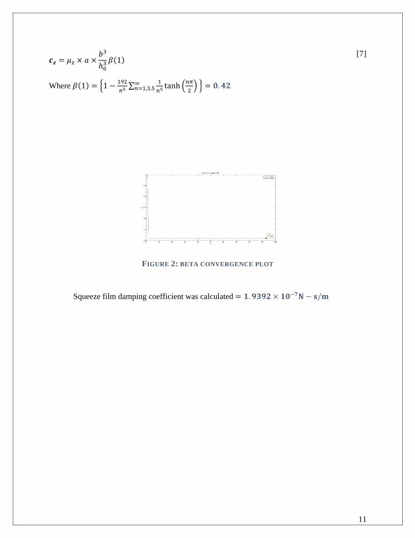
𝒄𝒄𝒛𝒛 = 𝜇𝜇𝑧𝑧 × 𝑎𝑎 ×𝑏𝑏3

ℎ03𝛽𝛽(1)

[7]

Where 𝛽𝛽(1) = �1 − 192𝜋𝜋5∑ 1

𝐾𝐾5tanh �𝐾𝐾𝜋𝜋

2� ∞

𝐾𝐾=1,3,5 � = 𝟑𝟑.𝟐𝟐𝟐𝟐

FIGURE 2: BETA CONVERGENCE PLOT

Squeeze film damping coefficient was calculated = 𝟖𝟖.𝟗𝟗𝟐𝟐𝟗𝟗𝟐𝟐 × 𝟖𝟖𝟑𝟑−𝟕𝟕𝟕𝟕 − 𝐬𝐬/𝐦𝐦

11

DRIVING FORCE The force required to drive the proof mass in constant motion is provided by comb drive as shown below. The fingers on the comb drive and the side of the proof mass increase the surface area of the capacitor, which increases the capacitance

FIGURE 3: COMB DRIVE

Capacitance of one finger of the proof mass is given by

𝐶𝐶 =2𝜖𝜖𝑟𝑟𝜖𝜖0𝑙𝑙ℎ

𝑔𝑔 [8]

Where 𝑙𝑙 is initial overlap between fingers of proof mass is, ℎ is the height of gyroscope and 𝑔𝑔 is the gap between the fingers. 𝜖𝜖0 and 𝜖𝜖𝑟𝑟 are absolute permittivity and dielectric constant

Electrostatic Force [9] on proof mass is given by

Energy stored in Capacitor 𝐸𝐸 =12𝐶𝐶𝑉𝑉2

𝐹𝐹 =

𝑑𝑑𝐸𝐸𝑑𝑑𝑥𝑥

=𝑛𝑛𝜖𝜖𝑟𝑟𝜖𝜖0𝑙𝑙ℎ

𝑔𝑔Δ𝑉𝑉2

𝑒𝑒𝑙𝑙𝑒𝑒𝑒𝑒𝑡𝑡𝑡𝑡𝑒𝑒𝑒𝑒 𝑒𝑒𝑡𝑡𝑛𝑛𝑚𝑚𝑡𝑡𝑎𝑎𝑛𝑛𝑡𝑡, 𝜖𝜖0 = 8.854 × 10−12 Fm−1

DC Voltage applied to the anchor of the proof mass, while an AC current is supplied to drive electrode[9]

𝐹𝐹 =𝑛𝑛𝜖𝜖𝑟𝑟𝜖𝜖0𝑙𝑙ℎ

𝑔𝑔(𝑉𝑉𝐷𝐷𝐷𝐷 + 𝑉𝑉𝐴𝐴𝐷𝐷)2

𝑉𝑉𝐴𝐴𝐷𝐷 = 𝑉𝑉0 sin(𝜔𝜔𝑡𝑡)

12

𝐹𝐹 =2𝑛𝑛𝜖𝜖𝑟𝑟𝜖𝜖0ℎ

𝑔𝑔𝑉𝑉𝐷𝐷𝐷𝐷𝑉𝑉0 sin(𝜔𝜔𝑡𝑡) [9]

𝐅𝐅 = 𝟐𝟐.𝟐𝟐𝟕𝟕𝟑𝟑𝟕𝟕 × 𝟖𝟖𝟑𝟑−𝟖𝟖 𝟕𝟕

NATURAL FREQUENCY The frequency with which undamped system vibrates

𝝎𝝎𝒙𝒙 = ��𝑘𝑘𝑥𝑥𝑒𝑒𝑒𝑒𝑒𝑒𝑚𝑚

� = 1.3859 × 105𝑡𝑡𝑎𝑎𝑑𝑑𝑚𝑚

= 𝟐𝟐𝟐𝟐𝟑𝟑𝟖𝟖𝟕𝟕𝟐𝟐𝒛𝒛

𝝎𝝎𝒛𝒛 = ��𝑘𝑘𝑧𝑧𝑒𝑒𝑒𝑒𝑒𝑒𝑚𝑚

� = 4.6195 × 104𝑡𝑡𝑎𝑎𝑑𝑑/𝑚𝑚 = 𝟕𝟕𝟐𝟐𝟕𝟕𝟕𝟕𝟐𝟐𝒛𝒛

DAMPING RATIO The damping ratio is a dimensionless measure describing how oscillations in a system decay after a disturbance. The damping ratio provides a mathematical means of expressing the level of damping in a system relative to critical damping. For a damped harmonic oscillator with mass m, damping coefficient c, and spring constant k, it can be defined as the ratio of the damping coefficient in the system's differential equation to the critical damping coefficient

𝜁𝜁 =𝑒𝑒𝑒𝑒𝑐𝑐

, 𝑒𝑒𝑐𝑐 = 2√𝑘𝑘𝑚𝑚

𝜻𝜻𝒙𝒙 =𝑒𝑒𝑥𝑥

2�𝑘𝑘𝑥𝑥𝑚𝑚= 𝟖𝟖.𝟖𝟖𝟖𝟖𝟕𝟕 × 𝟖𝟖𝟑𝟑−𝟖𝟖𝟐𝟐

𝜻𝜻𝒛𝒛 =𝑒𝑒𝑧𝑧

2�𝑘𝑘𝑧𝑧𝑚𝑚= 𝟕𝟕.𝟐𝟐𝟖𝟖𝟖𝟖𝟖𝟖 × 𝟖𝟖𝟑𝟑−𝟖𝟖𝟖𝟖

TABLE 1: LIST OF CONSTANTS

S.no Property x-direction z-direction

1 Mass (𝑘𝑘𝑔𝑔) 1.1650 × 10−8 1.1650 × 10−8

2 Spring constant (𝑁𝑁/𝑚𝑚) 223.75 24.8611

3 Damping Coefficient(𝑁𝑁 − 𝑚𝑚/𝑚𝑚) 2.3102 × 10−10 1.9392 × 10−7

4 Damping ratio 1.865 × 10−13 5.2181 × 10−11

5 Natural frequency (𝐻𝐻𝐻𝐻) 22067 7355

13

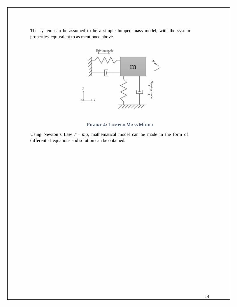
The system can be assumed to be a simple lumped mass model, with the system properties equivalent to as mentioned above.

FIGURE 4: LUMPED MASS MODEL

Using Newton’s Law F = ma, mathematical model can be made in the form of differential equations and solution can be obtained.

14

EQUATION OF MOTION Drive Axis (z-axis) The equation for damped system-mass system

𝑚𝑚𝑑𝑑2𝑥𝑥𝑑𝑑𝑡𝑡2

+ 𝑒𝑒𝑥𝑥𝑑𝑑𝑥𝑥𝑑𝑑𝑡𝑡

+ 𝑘𝑘𝑥𝑥𝑥𝑥 = 𝐹𝐹

𝑚𝑚𝑑𝑑2𝑥𝑥𝑑𝑑𝑡𝑡2

+ 𝑒𝑒𝑥𝑥𝑑𝑑𝑥𝑥𝑑𝑑𝑡𝑡

+ 𝑘𝑘𝑥𝑥𝑥𝑥 =2𝑛𝑛𝜖𝜖0ℎ𝑔𝑔

𝑉𝑉𝑑𝑑𝑐𝑐𝑣𝑣0 sin(𝜔𝜔𝑑𝑑𝑡𝑡)

𝑚𝑚𝑑𝑑2𝑥𝑥𝑑𝑑𝑡𝑡2

+ 𝑒𝑒𝑥𝑥𝑑𝑑𝑥𝑥𝑑𝑑𝑡𝑡

+ 𝑘𝑘𝑥𝑥𝑥𝑥 = 𝐴𝐴 sin(𝜔𝜔𝑑𝑑𝑡𝑡)

Using the natural frequency of the simple harmonic oscillator and damping ratio, we can rewrite this equation as

𝑑𝑑2𝑥𝑥𝑑𝑑𝑡𝑡2

+ 2𝜁𝜁𝑥𝑥𝜔𝜔𝐾𝐾𝑥𝑥𝑑𝑑𝑥𝑥𝑑𝑑𝑡𝑡

+ 𝜔𝜔𝐾𝐾𝑥𝑥2 𝑥𝑥 = 𝐴𝐴 sin𝜔𝜔𝑑𝑑𝑡𝑡 [10]

Where,

𝑨𝑨 = 𝟐𝟐𝟐𝟐𝝐𝝐𝟑𝟑𝝐𝝐𝒓𝒓𝒉𝒉𝒎𝒎𝒎𝒎

𝑽𝑽𝒅𝒅𝒄𝒄𝒗𝒗𝟑𝟑 [11]

Displacement in x-direction,

As General solution tends to 0 for over damped case, therefore, neglecting it. Taking particular solution of

𝑥𝑥 = 𝐴𝐴 sin𝜔𝜔𝑑𝑑 + 𝐵𝐵 cos𝜔𝜔𝑑𝑑 which can also be written as x = X cos(ωdt − ϕ)[10]

Where 𝑋𝑋 =𝐴𝐴

�(𝜔𝜔𝐾𝐾𝑥𝑥2 − 𝜔𝜔𝑑𝑑2)2 + (2𝜁𝜁𝑥𝑥𝜔𝜔𝐾𝐾𝑥𝑥𝜔𝜔𝑑𝑑)2

; tan𝜙𝜙 =2𝜁𝜁𝜔𝜔𝐾𝐾𝑥𝑥𝜔𝜔𝑑𝑑

𝜔𝜔𝐾𝐾𝑥𝑥2 − 𝜔𝜔𝑑𝑑2 [12]

Sense Axis (z-axis) Due to angular rate of device in y-axis, a Coriolis force is induced in z-axis. The force can be

given as 𝐹𝐹 = 2𝑚𝑚Ω × 𝑑𝑑𝑥𝑥𝑑𝑑𝑑𝑑

Where Ω is the angular velocity of device in y-axis

The equation of motion is similar to Drive equation

𝑚𝑚𝑑𝑑2𝐻𝐻𝑑𝑑𝑡𝑡2

+ 𝑒𝑒𝑦𝑦𝑑𝑑𝐻𝐻𝑑𝑑𝑡𝑡

+ 𝑘𝑘𝐻𝐻 = 2𝑚𝑚Ωdxdt

This can be rewritten as

15

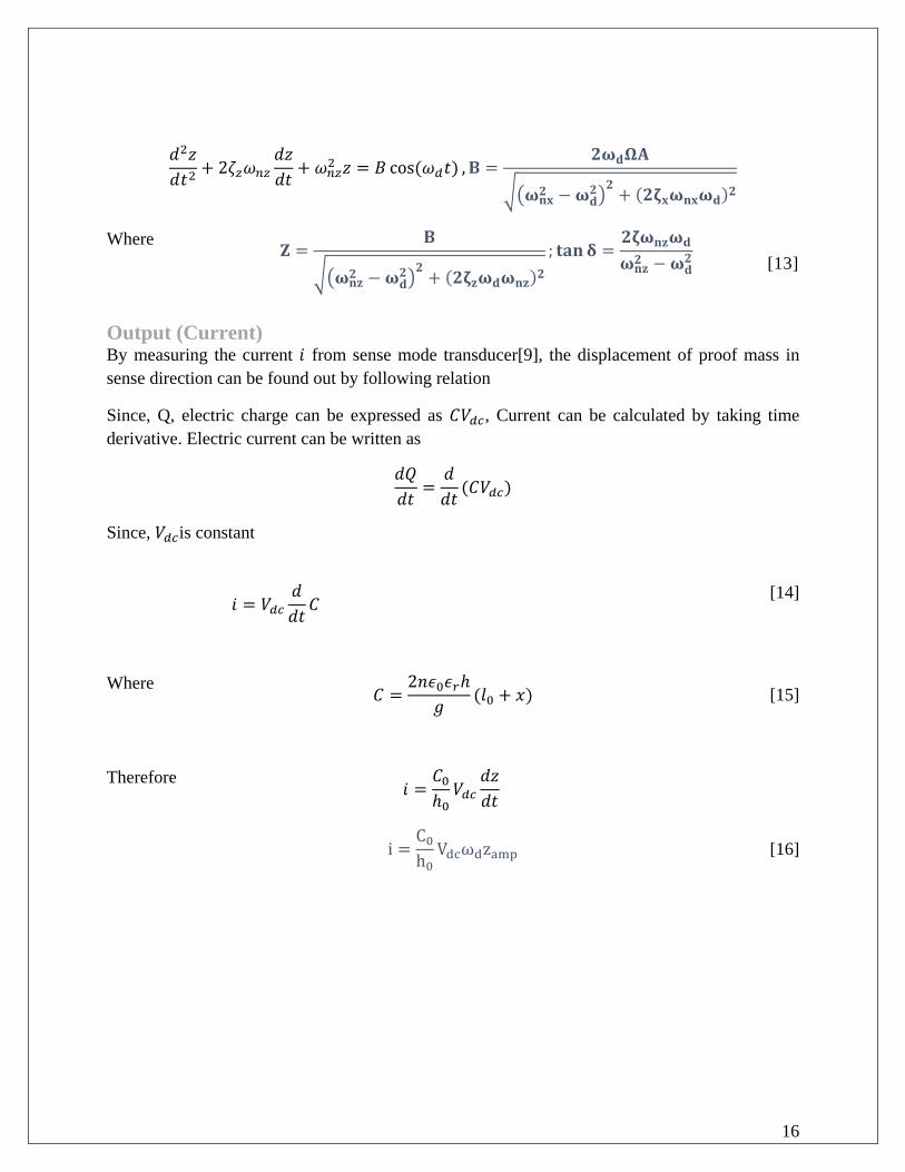
𝑑𝑑2𝐻𝐻𝑑𝑑𝑡𝑡2

+ 2𝜁𝜁𝑧𝑧𝜔𝜔𝐾𝐾𝑧𝑧𝑑𝑑𝐻𝐻𝑑𝑑𝑡𝑡

+ 𝜔𝜔𝐾𝐾𝑧𝑧2 𝐻𝐻 = 𝐵𝐵 cos(𝜔𝜔𝑑𝑑𝑡𝑡) ,𝐁𝐁 =𝟐𝟐𝛚𝛚𝐝𝐝𝛀𝛀𝛀𝛀

��𝛚𝛚𝐧𝐧𝐱𝐱𝟐𝟐 − 𝛚𝛚𝐝𝐝

𝟐𝟐�𝟐𝟐 + (𝟐𝟐𝛇𝛇𝐱𝐱𝛚𝛚𝐧𝐧𝐱𝐱𝛚𝛚𝐝𝐝)𝟐𝟐

Where 𝐙𝐙 =𝐁𝐁

��𝛚𝛚𝐧𝐧𝐳𝐳𝟐𝟐 − 𝛚𝛚𝐝𝐝

𝟐𝟐�𝟐𝟐 + (𝟐𝟐𝛇𝛇𝐳𝐳𝛚𝛚𝐝𝐝𝛚𝛚𝐧𝐧𝐳𝐳)𝟐𝟐; 𝐭𝐭𝐭𝐭𝐧𝐧𝛅𝛅 =

𝟐𝟐𝛇𝛇𝛚𝛚𝐧𝐧𝐳𝐳𝛚𝛚𝐝𝐝

𝛚𝛚𝐧𝐧𝐳𝐳𝟐𝟐 − 𝛚𝛚𝐝𝐝

𝟐𝟐 [13]

Output (Current) By measuring the current 𝑒𝑒 from sense mode transducer[9], the displacement of proof mass in sense direction can be found out by following relation

Since, Q, electric charge can be expressed as 𝐶𝐶𝑉𝑉𝑑𝑑𝑐𝑐, Current can be calculated by taking time derivative. Electric current can be written as

𝑑𝑑𝑑𝑑𝑑𝑑𝑡𝑡

=𝑑𝑑𝑑𝑑𝑡𝑡

(𝐶𝐶𝑉𝑉𝑑𝑑𝑐𝑐)

Since, 𝑉𝑉𝑑𝑑𝑐𝑐is constant

𝑒𝑒 = 𝑉𝑉𝑑𝑑𝑐𝑐𝑑𝑑𝑑𝑑𝑡𝑡𝐶𝐶

[14]

Where 𝐶𝐶 =

2𝑛𝑛𝜖𝜖0𝜖𝜖𝑟𝑟ℎ𝑔𝑔

(𝑙𝑙0 + 𝑥𝑥) [15]

Therefore 𝑒𝑒 =

𝐶𝐶0ℎ0𝑉𝑉𝑑𝑑𝑐𝑐

𝑑𝑑𝐻𝐻𝑑𝑑𝑡𝑡

i =C0h0

Vdcωdzamp [16]

16

RESULTS Amplitude v/s frequency response was plotted; Maximum Amplitude was obtained at lower natural frequency of the x and z directions. (𝜔𝜔𝑧𝑧 =7355𝐻𝐻𝐻𝐻)

Device was simulated at 𝜔𝜔𝑑𝑑 = 7355𝐻𝐻𝐻𝐻

Response of amplitude v/s Angular rate was compared between square beam and rectangular beam with dimensions 5𝜇𝜇𝑚𝑚 and 5𝜇𝜇𝑚𝑚 𝑎𝑎𝑛𝑛𝑑𝑑 15𝜇𝜇𝑚𝑚 respectively.

FIGURE 4: DRIVE FREQUENCY V/S AMPLITUDE RESPONSE IN SENSE DIRECTION

Omega=7355

17

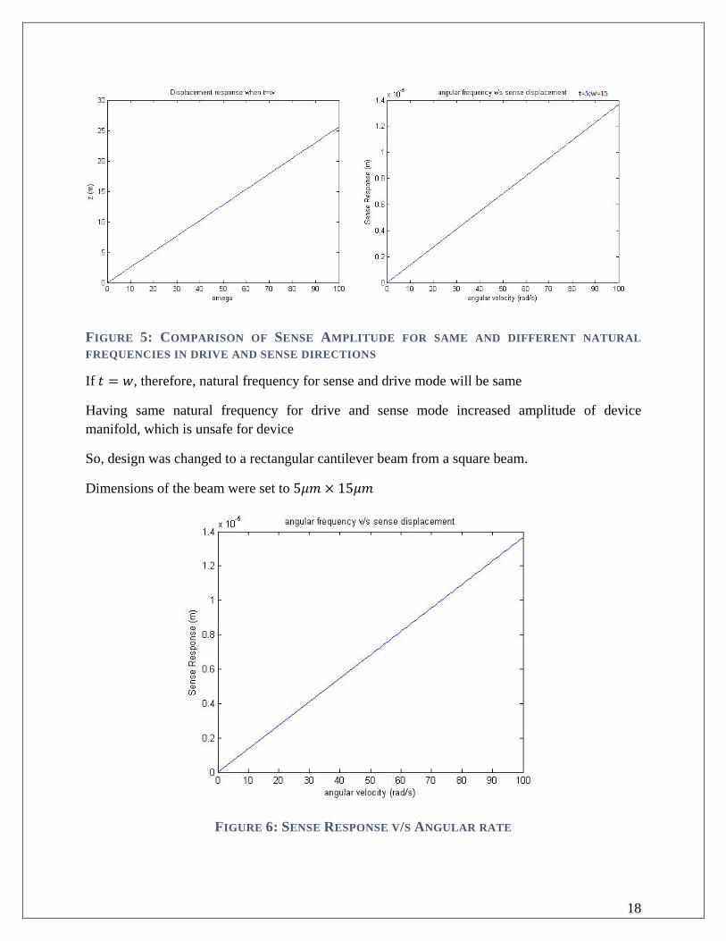
FIGURE 5: COMPARISON OF SENSE AMPLITUDE FOR SAME AND DIFFERENT NATURAL FREQUENCIES IN DRIVE AND SENSE DIRECTIONS

If 𝑡𝑡 = 𝑤𝑤, therefore, natural frequency for sense and drive mode will be same

Having same natural frequency for drive and sense mode increased amplitude of device manifold, which is unsafe for device

So, design was changed to a rectangular cantilever beam from a square beam.

Dimensions of the beam were set to 5𝜇𝜇𝑚𝑚 × 15𝜇𝜇𝑚𝑚

FIGURE 6: SENSE RESPONSE V/S ANGULAR RATE

18

Transducers are used in sense axis which uses current output to measure the sense displacement

By [17] Current v/s Angular velocity was plotted to get the sensitivity of the device.

Sensitivity is defined as 𝑆𝑆 = 𝑐𝑐ℎ𝑎𝑎𝐾𝐾𝑎𝑎𝑒𝑒 𝑖𝑖𝐾𝐾 𝑐𝑐𝑐𝑐𝑟𝑟𝑟𝑟𝑒𝑒𝐾𝐾𝑑𝑑 𝑚𝑚𝑎𝑎𝑎𝑎𝐾𝐾𝑖𝑖𝑑𝑑𝑐𝑐𝑑𝑑𝑒𝑒𝑐𝑐ℎ𝑎𝑎𝐾𝐾𝑎𝑎𝑒𝑒 𝑖𝑖𝐾𝐾 𝑎𝑎𝐾𝐾𝑎𝑎𝑐𝑐𝑎𝑎𝑎𝑎𝑟𝑟 𝑣𝑣𝑒𝑒𝑎𝑎𝑣𝑣𝑐𝑐𝑖𝑖𝑑𝑑𝑦𝑦

which is equal to slope the curve.

Sensitivity of this device was found out to be 𝟐𝟐.𝟐𝟐 × 𝟖𝟖𝟑𝟑−𝟖𝟖 𝛀𝛀/ �𝐫𝐫𝐭𝐭𝐝𝐝𝐬𝐬�−𝟖𝟖

FIGURE 7: SENSE CURRENT V/S ANGULAR RATE

19

BIBLIOGRAPHY

[1] A. A. Trusov, “Overview of MEMS Gyroscopes : History , Principles of Operations , Types of Measurements,” Irvine,CA,USA, 2011.

[2] S. Nasiri and S. Clara, “A Critical Review of MEMS Gyroscopes Technology and Commercialization Status,” Avaliable online http//invensense.com/mems/gyro/documents/whitepapers/MEMSGyroComp. pdf (accessed 25 May 2012), p. 8, 2009.

[3] A. Burg, A. Meruani, A. Sandheinrich, and M. Wickmann, “MEMS Gyroscopes and their Applications,” Introd. to Microelectromechanical Syst., 2011.

[4] J. E. Shigley, C. R. Mischke, R. G. Budynas, and K. J. Nisbett, Mechanical Engineering Design, 8th ed. New York: McGraw-Hill, 2010.

[5] H. K. Sharma, A. Jain, and R. Gopal, “Estimation of slide film damping in laterally moving microstructures using FEM simulations,” in National Conference on Innovations in Microelectronics, Signal and Communication Technologies, 2014.

[6] J. A. Fay, Introduction to Fluid Mechanics. New Delhi: PHI Learning Private Limited, 2012.

[7] H. K. Sharma, A. Jain, and R. Gopal, “FEM simulations for estimating squeeze film damping in microstructures,” in International Conference on Advance Trends in Engineering and Technology, 2013, pp. 112–114.

[8] M. Bao and H. Yang, “Squeeze film air damping in MEMS,” Sensors Actuators, A Phys., vol. 136, no. 1, pp. 3–27, 2007.

[9] A. Bristow, T. Barton, and S. Nary, “MEMS Tuning-Fork Gyroscope Final Report.”

[10] H. Dong and X. Xiong, “Design and Analysis of a MEMS Comb Vibratory Gyroscope,” in UB - NE ASEE 2009 Conference, 2009, p. 12.

20

APPENDIX Code 𝛽𝛽 Equation was solved in MATLAB file beta1.m

rat=1; c=0; for i=1:100 g=2*i-1; beta=1-(192/3.14^5)*c/rat; b1 = (1/g^5)*tanh(g*3.14*rat/2); y(i)=beta; x(i)=i; c=b1+c; end

FIGURE 8: CODE FOR BETA CONVERGENCE

21

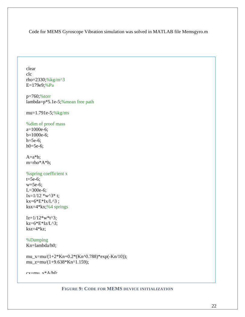
Code for MEMS Gyroscope Vibration simulation was solved in MATLAB file Memsgyro.m

clear clc rho=2330;%kg/m^3 E=179e9;%Pa p=760;%torr lambda=p*5.1e-5;%mean free path mu=1.791e-5;%kg/ms %dim of proof mass a=1000e-6; b=1000e-6; h=5e-6; h0=5e-6; A=a*b; m=rho*A*h; %spring coefficient x t=5e-6; w=5e-6; L=300e-6; Ix=1/12 *w^3* t; kx=6*E*Ix/L^3 ; ksx=4*kx;%4 springs Iz=1/12*w*t^3; kz=6*E*Iz/L^3; ksz=4*kz; %Damping Kn=lambda/h0; mu_x=mu/(1+2*Kn+0.2*(Kn^0.788)*exp(-Kn/10)); mu_z=mu/(1+9.638*Kn^1.159); cx=mu x*A/h0;

FIGURE 9: CODE FOR MEMS DEVICE INITIALIZATION

22

zx=cx/2*sqrt(ksx*m); zz=cz/2*sqrt(ksz*m); %natural freq nfx=sqrt(ksx/m); nfz=sqrt(ksz/m); %force n=10; ep=8.854e-12*1.0053; Vdc=10; V0=10; g=2e-6; %gap bw combs F=2*n*ep*h*Vdc*V0/g; ohm=2; for p=1:108000 f(p)=p/(2*3.14); Ax(p)=abs(F/(m*sqrt((nfx^2-p^2)^2+(2*zx*p)^2))); Az(p)=abs(2*ohm*p*Ax(p)/sqrt((nfz^2-p^2)+(2*zz*p)^2)); end plot(f,Az) anfx=nfx/(2*3.14); anfz=nfz/(2*3.14); aaaz=max(Az); aaanf=find(Az==aaaz)/(2*3.14); %Capacitance C0=ep*a*b/h0; clear ohm p for p=1:101 ohm(p)=p-1; fd=aaanf*2*3.14; Axd(p)=abs(F/(m*sqrt((nfx^2-fd^2)^2+(2*zx*fd)^2))); Azd(p)=abs(2*ohm(p)*fd*Axd(p)/sqrt((nfz^2-fd^2)+(2*zz*fd)^2)); Current(p)=(C0/h0)*fd*Azd(p)*Vdc; end plot(ohm,Azd) phi=2*zx*nfx*fd/(nfx^2-fd^2); del=2*zz*nfz*fd/(nfz^2-fd^2); tphi=atand(phi); tdel=atand(del);

FIGURE 10: CODE FOR MEMS DEVICE VIBRATION ANALYSIS

23