Melt Scheduling to Trade-Off Material Waste and Shipping Performance

Kedar S. NaphadeBell Laboratories, Lucent Technologies

S. David Wu and Robert H. StorerManufacturing Logistics Institute, Lehigh University

Bhavin J. DoshiCAPS Logistics

ABSTRACT

The ingot formation or “melt” process is the first step in many steel making operations. This processinvolves melting steel and alloys for desired chemical composition, then pouring it into a variety ofingot molds. Complex technological and resource constraints can make the planning and schedulingof such processes extremely challenging. In this paper, we report our experience in developingsolution methods for this “melt scheduling” problem at BethForge, a division of the Bethlehem SteelCorporation, and a manufacturer of custom-made heavy steel forgings. We describe the main issuesassociated with generic melt scheduling problem as well as constraints that are specific to BethForge.The problem at BethForge is particularly challenging due to the need to keep the ingot at a hightemperature before forging, their high product variety, and the need to consider trade-offs betweentwo conflicting objectives. We first formulate the base melt scheduling problem as a mixed integerprogram. We then decouple the scheduling decisions into two levels and develop a local searchalgorithm based on Storer and Wu’s problem space neighborhood. Our aim is to generate a familyof efficient schedules that allow decision makers to balance the tradeoff between two criteria.Computational experiments are performed using data from BethForge. The melt scheduling proceduredeveloped herein has been implemented and installed at BethForge. It made fundamentalimprovement in their melt scheduling process.

1

Steel ingots form the raw material for a variety of steel products that are processed through

forging, heat treatment and other similar steel manufacturing processes. Steel manufacturers either

have ingots delivered to them or have ingot formation processes at the front end of the plant. The

ingot formation or “melt” process is extremely critical because of its capital and energy intensive

nature, and the effect it has on the material flow of the downstream production processes. These

factors, coupled with a complex set of resource and technological constraints, make melt scheduling

a very challenging problem. When we started our study at BethForge in 1995 melt scheduling was

carried out manually by seasoned schedulers who were intimately familiar with the complex

engineering rules and constraints involved in the process. Later in 1995, Bethlehem Steel decided

to move the melt operation from within the Bethlehem plant to Steelton, PA (some 80 miles away),

where ingots for other steel products are also poured. The forging, heat treatment and machining

processes remain in the Bethlehem plant. Steel ingots are poured on a weekly basis at Steelton, then

transported by rail carts to Bethlehem. This new process creates major challenges to the manual

scheduling system as the melt operation is now limited to a specific time slot during the week, strict

weight restrictions are imposed by the Steelton melting resources, and frequent rescheduling becomes

necessary due to variations in crew configuration, maintenance plan, resource availability, and rail

transportation constraints. Our study herein is part of a joint NSF/Private sector research initiative

where we seek to restructure and develop more robust and practical solutions for production

scheduling in industry. In Naphade et al. (1996) and Doshi et al. (1996) some of the preliminary

results in melt scheduling at BethForge were documented. The proposed melt scheduling procedure

has been coded, tested and demonstrated to BethForge management. The procedure has later been

integrated into their planning and scheduling system. In this paper we report in detail our experience

in developing the overall solution methodology for this particular problem and computational results

obtained for real instances at BethForge. The paper is organized as follows: Section 1 explains the

process of steel ingot formation, Section 2 provides a detailed description on the melt scheduling

problem at BethForge, Section 3 present a MIP formulation for the stated melt scheduling problem,

and Section 4 describe a two-level heuristic for the solution of the problem. In Section 5 we presents

computational experiments using actual order data, and in Section 6 we discuss experiences and

insights gained from implementing the scheduling system at BethForge.

1. The Ingot Formation Process

The ingot formation process typically consists of four steps as shown in Figure 1. The first

operation in the process is melting steel scrap in an electric arc furnace (EAF). The molten metal is

TankDegasser

Ladle FurnaceLadle

EAF

Pour Plates

2

Ingot Formation ProcessFigure 1

then transferred in a ladle to a ladle furnace where alloying elements are added. The next step is tank

degassing in which gases are removed from the metal to avoid porosity and air bubbles inside the final

ingot which could adversely affect the material properties. Finally the molten metal is poured

onto bottom pour plates or top pour tanks in which it solidifies to a cylindrically shaped ingot. There

are several constraints associated with processes of this type which can be characterized by three

basic factors: capacity of the metal-melting furnace(s), specific dimensions of the molds and plates,

and chemical compositions of different ingots. For the convenience of discussion, we loosely group

the constraints into two: constraints associated with the furnace (EAF Constraints) and constraints

associated with the molds (Pour Constraints).

EAF Constraints

EAF constraints result from the operating characteristics of the electric arc furnace. Firstly

the furnace operates within a certain capacity interval, where the capacity is defined as the total

3

weight of the metal that can be melted in one furnace load. The upper capacity limit is due to the

physical size of the furnace. The lower capacity limit arises due to the fact that the electrodes in an

EAF must be dipped into the metal to a sufficient depth in order to facilitate efficient heat transfer

through the steel (see Figure 1). A load of metal scrap melted in the furnace is called a “heat”. Several

ingots may be poured from a single heat. However all ingots that are poured from a heat have to be

of the same basic chemical composition, or “grade.” Thus for each heat one needs to identify a

specific subset of ingots from the current order pool which have a common grade and at the same

time a total weight within the capacity interval for the furnace. We refer to the above process as the

“heat packing” problem. Clearly if there are a large number of orders, or there is more than one

furnace and the different furnaces have different capacity intervals, one needs to examine a fairly large

number of alternative solutions.

Pour Constraints

After refining and degassing of a particular heat, the molten metal is poured into “bottom

pour” plates or “top pour” tanks. The terms top-pour and bottom-pour refer to the mechanism in

which molten metal rises on the plates for solidification. Bottom pour are typical for smaller size

ingots where the molten metal is poured via a down fountain into connected channels (or “runners”)

built into a plate. The metal then rises up to the desired height in each ingot mold on the plate. For

top pour operations the molten metal is simply poured top down into the mold. Typically pour

constraints arise out of three different considerations: number of holes (mold positions) on a plate,

different sizes of ingots molds that could be mounted on a given plate, and chemical grade of ingots

to be poured (this is only an issue when more than one heat is needed to pour the ingots on a same

plate). Several different types of plates with overlapping diameter ranges may be available with a

varying number of holes on each plate. After a heat is formed, assigning particular plates to desired

ingots is a non-trivial resource allocation problem since all physical specifications must be met. This

is further compounded by the issue of “blockable” or “non-blockable” runners. As described earlier,

runners are channels that connect the down fountain with mold positions. If a plate has blockable

runners, it means that the ingots poured onto that plate could be of several different grades and

heights. On the other hand, for plates without blockable runners, metal is free to mix and hence all

ingots need to be of the same grade and same height.

The above EAF constraints and pour constraints can be expected, with some minor

variations, in any ingot formation processes. What is likely to vary from one melt shop to another

4

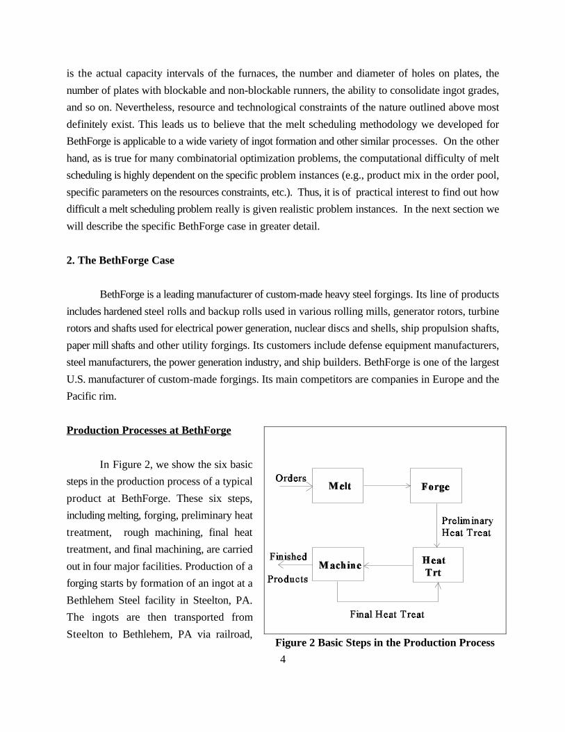
Figure 2 Basic Steps in the Production Process

is the actual capacity intervals of the furnaces, the number and diameter of holes on plates, the

number of plates with blockable and non-blockable runners, the ability to consolidate ingot grades,

and so on. Nevertheless, resource and technological constraints of the nature outlined above most

definitely exist. This leads us to believe that the melt scheduling methodology we developed for

BethForge is applicable to a wide variety of ingot formation and other similar processes. On the other

hand, as is true for many combinatorial optimization problems, the computational difficulty of melt

scheduling is highly dependent on the specific problem instances (e.g., product mix in the order pool,

specific parameters on the resources constraints, etc.). Thus, it is of practical interest to find out how

difficult a melt scheduling problem really is given realistic problem instances. In the next section we

will describe the specific BethForge case in greater detail.

2. The BethForge Case

BethForge is a leading manufacturer of custom-made heavy steel forgings. Its line of products

includes hardened steel rolls and backup rolls used in various rolling mills, generator rotors, turbine

rotors and shafts used for electrical power generation, nuclear discs and shells, ship propulsion shafts,

paper mill shafts and other utility forgings. Its customers include defense equipment manufacturers,

steel manufacturers, the power generation industry, and ship builders. BethForge is one of the largest

U.S. manufacturer of custom-made forgings. Its main competitors are companies in Europe and the

Pacific rim.

Production Processes at BethForge

In Figure 2, we show the six basic

steps in the production process of a typical

product at BethForge. These six steps,

including melting, forging, preliminary heat

treatment, rough machining, final heat

treatment, and final machining, are carried

out in four major facilities. Production of a

forging starts by formation of an ingot at a

Bethlehem Steel facility in Steelton, PA.

The ingots are then transported from

Steelton to Bethlehem, PA via railroad,

5

using specially designed rail cars. The next process is hot forging at the press forge. The forged ingots

then go to the treatment shop where they undergo a cycle of preliminary heat treatment. The so-called

"hot-end" consists of all the shops up to and including the treatment shop. Ingots must be kept at a

high temperature the whole time while they are in the hot-end. From the treatment shop, the ingots

visit one of two machining shops where they undergo rough machining. Some of the products from

machine shop revisit the treatment shop for final heat treatment, this is followed by finish machining

to their final dimensions and surface specifications. Though the melt operation does not actually take

place in Bethlehem, the facility at Steelton has a dedicated number of shifts (each week) and resources

allocated to BethForge ingots. BethForge is responsible for scheduling its own melting operations

on those resources during the designated shifts on a weekly basis. In the following, we describe in

detail the specific constraints and managerial objectives for this melt scheduling problem.

EAF Constraints at Steelton

We have described earlier the general EAF constraints due to furnace capacity range and

grade compatibility. At Steelton one specific electrical arc furnace is dedicated for BethForge

Products. Six to seven heats can be melted in this furnace during the shifts dedicated to BethForge

each week. The operational capacity for this furnace has a lower weight limit of 125 tons and an

upper limit of 145 tons. As mentioned previously, this means that for each heat the scheduler must

identify a subset of ingots from the order pool which has a total weight lying between these limits.

Each ingot(s) specified in an order has a promised delivery date (due-date). Clearly all ingots in the

order pool must be produced eventually. Ingots for BethForge products weigh from as low as 12

tons (Harden Steel Rolls, or HSRs) to as high as 200 tons (Backup Rolls). The grades for the lighter

HSR’s usually differ from the grades of heavier ingots implying that HSRs cannot be packed into the

same heat with the heavier ingots. Most ingots that could be packed into the same heat (that are of

the same grade) weigh between 30 and 110 tons. Packing these ingots to fit into the narrow capacity

interval is quite a challenge. Ingots weighing more than 145 tons are usually poured from two heats.

For these ingots there are some additional pour constraints which we will discuss further in the next

section.

There is an important cost implication associated with the heat packing decision for the EAF.

Recall that the EAF has a lower weight limit of 125 tons. Consider a scenario where an ingot has a

total weight of 110 tons. Unless there is an ingot of the same grade which has a weight between 15

to 35 tons, 125 tons of metal must be melted in the heat and the extra 15 tons of metal is wasted.

Waste of molten metal is extremely expensive and minimizing waste is one of the primary objectives

6

of this scheduling problem.

Ingots weighing over 145 tons need to be poured jointly from two heats (there are no ingots

weighing more than 290 tons). Molten metal from the first heat is stored in the ladle furnace while

the second heat is melted. Hence if an ingot is to be split between two heats, the two heats must be

consecutive. Additional technological constraints prevent splitting of two ingots into three or more

consecutive heats, e.g., if there are two ingots of 200 tons each, pouring the first ingot for the first

two heats and the second ingot for the second and third heats is not technologically feasible.

Pour Constraints at Steelton

There are three basic types of pour resources. The largest ingots (> 92" dia) are poured into

top pour plates (Type 1 plates). Two such plates are available and each can accommodate one ingot

each. The second type of pour resource is a bottom pour plate with blockable runners. Ingots of

different grades ranging in diameter from 54" to 92" can be poured on these plates. The plates are

further divided by two diameter ranges, types 2A (54" to 78") and 2B (69" to 92"). The third

resource is bottom-pour plates with non-blockable runners. These are used for ingots of the same

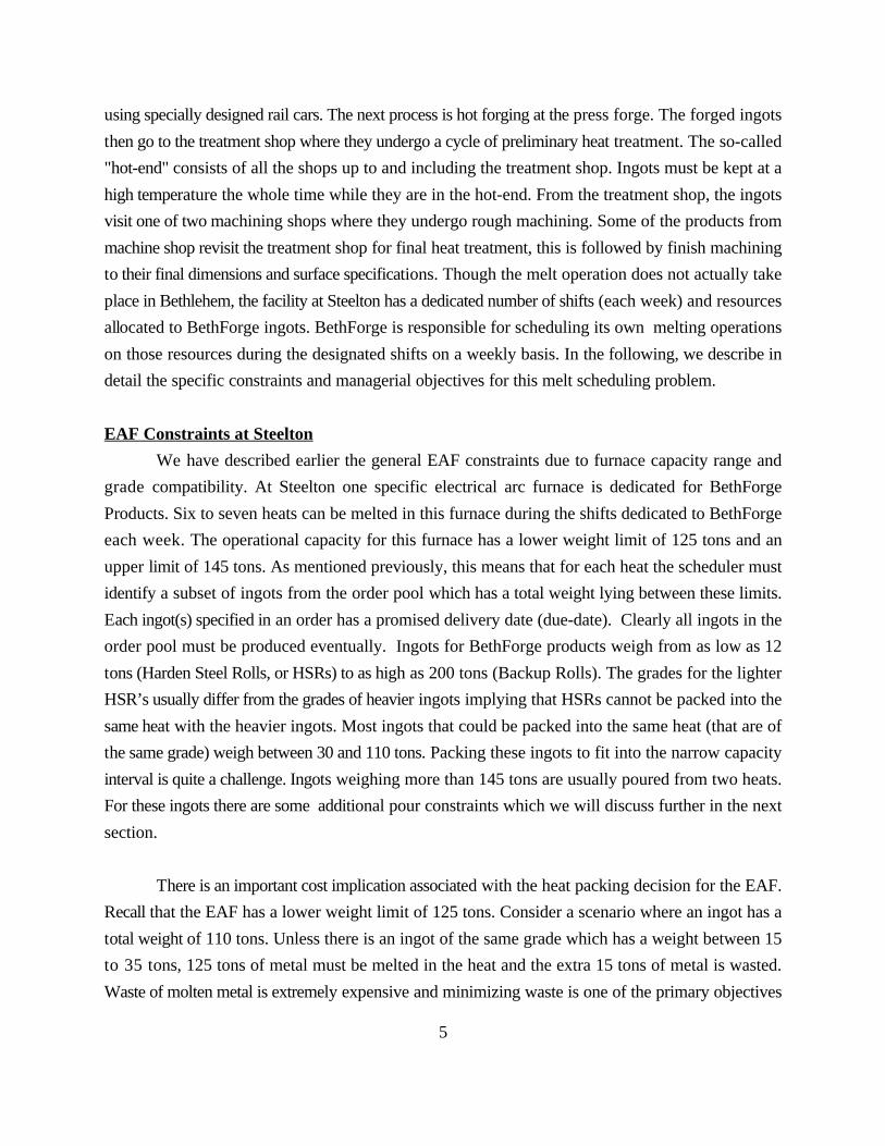
grade ranging from 40" to 48" in diameter. Table 1 summarizes the plate diameter ranges and

characteristics. Table 2 summarizes the ingots and plates compatibility information. It is clear that for

ingots in the ranges 40" to 48" and > 92" only one particular plate can be used for a particular grade

at any one time. The selection of ingots for a plate is therefore independent between different grades.

On the other hand, for ingots between 54" to 92", the selection of ingots for a plate must take into

consideration all eligible ingots.

Table 1 Ingot Pouring Resources

Plate Type Diameter Range No. available No. of holes/plate

1 > 54" 2 1

2A 69" - 92" 2 2

2B 54" - 78" 2 2

3 40" - 48" 4 6

The Zero WIP Constraint

Perhaps the most restrictive among all constraints at BethForge is the zero-WIP constraint.

7

This constraint states that any metal that is melted in the EAF has to be poured in the same period.

Thus all molten steel will either be poured as ingots or will be wasted. This constraint is significant

as it links directly the EAF and Pour constraints. In other words, as we select a set of ingots to be

processes during a week, EAF and Pour constraints must be satisfied simultaneously. For instance,

suppose there are four 35-ton ingots to be formed but there are only three positions available for the

respective diameter ranges on the pour plates. The Zero WIP constraint does not allow melting unless

the melted heat can be poured. Consequently one of the four ingots has to be removed from the heat

which then reduce the total heat weight below 125 tons leading to waste. These restrictive constraints

are precisely what make the melt scheduling problem difficult.

Table 2 Ingot-Plate Compatibility

Plate Resources

Ingot Diameter Range 1 2A 2B 3

40"- 48" 0 0 0 1

54" - 69" 1 0 1 0

9" - 78" 0 1 1 0

78" - 92" 1 1 0 0

> 92" 1 0 0 0

Release Dates and Due Dates

The melt scheduling problem is dynamic in that orders arrive continuously throughout the

year. When BethForge receives an inquiry for a product from a customer, there is a standard due-date

and price quotation process. After an agreement with the customer is reached, the detailed planning

of the product (including ingot design) is carried out. After this preliminary phase, the order is

released to the general “order pool” and the ingots specified in the order become candidates for

melting at Steelton. Thus with every ingot there is a specific release date and due date.

2.2 Objectives and Problem Statement

It is not difficult to see that waste minimization is an important objective for the melt

scheduling problem. Another important objective is to minimize order tardiness. There is a clear

conflict between the two objectives. In order to minimize material waste, one would try to search

for specific subset of ingots of the same grade from the order pool that have a total weight between

8

125 and 145 tons or 250 and 290 tons (as ingots may be split into two consecutive heats). If tardiness

is not a concern one may choose to combine any ingots of the same grade in the entire order pool,

or even wait for new orders. Unfortunately order tardiness is very much a concern and hence one may

be forced to accept some material waste in the interest of reducing order tardiness. We now

summarize intuitively the melt scheduling problem as follows:

Consider the set of ingots specified by the current order pool, each with weight, diameter,grade, order release date, and due-date information. Determine subsets of ingots to beprocessed in each of the next T weeks where each weekly subset contains H ingot groupings.T is a sufficiently large number to process all the ingots currently in the order pool and H isthe total number of heats available each week. Each ingot group represents ingots which canbe melted in a heat and poured onto available pour resources without violating any EAF andpour constraints. The objective is to minimize material waste and total order tardiness.

Related Literature

The literature dealing with scheduling problems for steel manufacturing process is quite

sparse. Existing methods that directly address complex, process-related constraints are mostly AI-

based, constraint satisfaction heuristics (c.f., Numao and Morishita, 1989; Minton, et al., 1989; Dorn

and Slany, 1994). Also relevant to this research is the issue of due-date determination and the

interaction of due-date performance with the scheduling procedure, this is the case since the due-

dates quoted could directly affect the degree of flexibility allowed in the melt scheduling problem and

the ultimate due-date performance. Although in reality due-dates are largely dictated by the

competition and the customer’s needs, the manufacturer does have limited control over due-date

setting. There is an extensive literature on due-date setting for scheduling problems. Cheng and

Gupta (1989) provide a intensive survey on due-date determination for production scheduling

problems. Dellaert (1991) demonstrated the interesting relationship between due-date setting and

production control policies. Cheng (1994) and Luss and Rosenwein (1993) examine ways to

optimize due-date assignment in manufacturing environments. Baker, (1984), Wein (1991) and Via

and Dolley (1991) examine the interaction and integration of due-date setting policies and scheduling

procedures. Ozdamar and Yazgac (1997) and Udo (1993) examine the relationship between

manufacturing capacity and due-date setting policies. Duenyas (1995) provides a different

perspective by examining due-date setting policies corresponding to different customer classes. De

et al. (1994) study due-date assignment and the performance of early/tardy scheduling. As we will

demonstrate in the computational experiments, in addition to external due-date quotation, internal

due-date setting to guarantee performance for a certain customers could have a profound impact on

overall scheduling performance as well.

9

Since ingot orders slowly come into the system over the course of a year, a melt schedule can be

implemented in a rolling horizon basis where each implementation is generated based on a snapshot

of the order pool. There is an extensive literature on various aspects of rolling horizon scheduling.

Stauffer and Liebling (1997) examine the scheduling problem in a rolling mill using a rolling horizon

implementation. Sethi and Sorger (1991), Uzsoy and Ovacik (1994), Chand et al.(1997) establish

some theoretic basis for rolling horizon scheduling and examine different execution policies. Russell

and Urban (1993) study the effects of rolling horizon window sizes. We have performed some limited

testing on the effect of rolling horizon implementation for melt scheduling. Apart from typical rolling

horizon issues, the primary goal here is to find new orders that would match the chemical grades and

sizes of existing ingots and form more efficient (lower waste) heats.

3. The MIP Formulation

In this section we present a mixed integer programming formulation of the BethForge melt

scheduling problem. The model helps identifying key decisions and parameters of the problem.

N total number of ingots (in the order pool) to be melted and poured P total number of platesW physical weight of ingot k (in tons) k

G grade of ingot k k

D diameter of ingot k k

dd due date of ingot k k

r release date of ingot kk

M 0-1 matrix of compatibility between ingot diameter and plate; M = 1, if diameter d can be accommodated on plate pdp

= 0, otherwise.C plate capacity; number of ingots that can be poured on plate p p

T total number of weeks in the planning horizonH maximum number of heats to be melted each weekMAXWT upper weight limit that can be melted in each heat; 145 tons in BethForge caseMINWT lower weight limit that can be melted in each heat; 125 tons in BethForge caseDecision Variables:* fraction of ingot k melted in heat h of week tkht

x a 0-1 variable indicating if metal from heat h of week t is used to pour ingot kkht

y a 0-1 variable that indicates whether ingot k is poured in week tkt

z a 0-1 variable that indicates whether ingot k is poured on plate p in week tkpt

f finish date of ingot k; it is the week in which ingot k is meltedk

T amount of waste in heat h of week tht

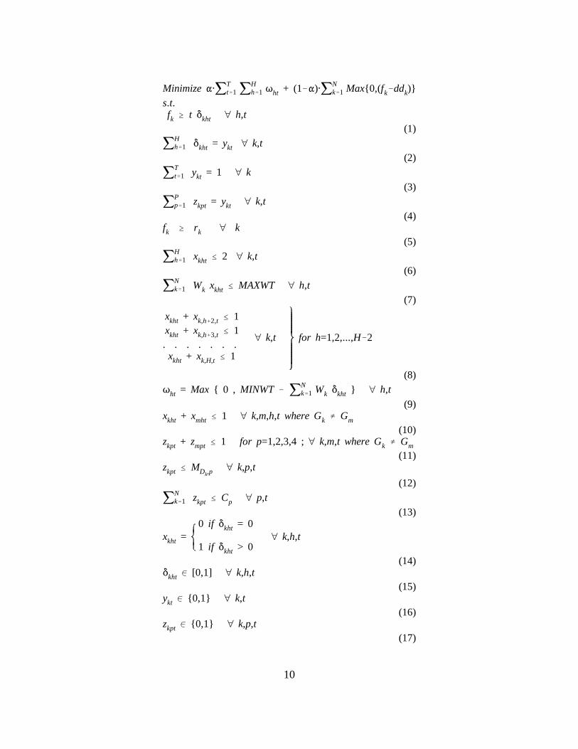
Minimize "@jTt'1 jH

h'1 Tht + (1!")@jNk'1 Max{0,(fk&ddk)}

s.t.fk $ t *kht œ h,t

(1)

jHh'1 *kht = ykt œ k,t

(2)

jTt'1 ykt = 1 œ k

(3)

jPp'1 zkpt = ykt œ k,t

(4)fk $ rk œ k

(5)

jHh'1 xkht # 2 œ k,t

(6)

jNk'1 Wk xkht # MAXWT œ h,t

(7)

xkht + xk,h%2,t # 1xkht + xk,h%3,t # 1. . . . . . .

xkht + xk,H,t # 1

œ k,t for h=1,2,...,H&2

(8)Tht = Max { 0 , MINWT ! jN

k'1 Wk *kht } œ h,t

(9)xkht + xmht # 1 œ k,m,h,t where Gk … Gm

(10)zkpt + zmpt # 1 for p=1,2,3,4 ; œ k,m,t where Gk … Gm

(11)zkpt # MDk,p

œ k,p,t

(12)

jNk'1 zkpt # Cp œ p,t

(13)

xkht =0 if *kht = 0

1 if *kht > 0œ k,h,t

(14)*kht 0 [0,1] œ k,h,t

(15)ykt 0 {0,1} œ k,t

(16)zkpt 0 {0,1} œ k,p,t

(17)

10

11

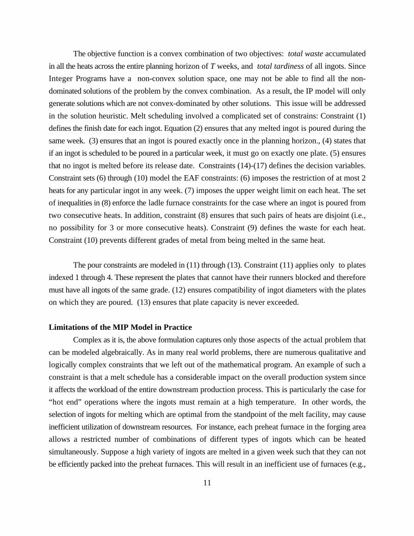
The objective function is a convex combination of two objectives: total waste accumulated

in all the heats across the entire planning horizon of T weeks, and total tardiness of all ingots. Since

Integer Programs have a non-convex solution space, one may not be able to find all the non-

dominated solutions of the problem by the convex combination. As a result, the IP model will only

generate solutions which are not convex-dominated by other solutions. This issue will be addressed

in the solution heuristic. Melt scheduling involved a complicated set of constrains: Constraint (1)

defines the finish date for each ingot. Equation (2) ensures that any melted ingot is poured during the

same week. (3) ensures that an ingot is poured exactly once in the planning horizon., (4) states that

if an ingot is scheduled to be poured in a particular week, it must go on exactly one plate. (5) ensures

that no ingot is melted before its release date. Constraints (14)-(17) defines the decision variables.

Constraint sets (6) through (10) model the EAF constraints: (6) imposes the restriction of at most 2

heats for any particular ingot in any week. (7) imposes the upper weight limit on each heat. The set

of inequalities in (8) enforce the ladle furnace constraints for the case where an ingot is poured from

two consecutive heats. In addition, constraint (8) ensures that such pairs of heats are disjoint (i.e.,

no possibility for 3 or more consecutive heats). Constraint (9) defines the waste for each heat.

Constraint (10) prevents different grades of metal from being melted in the same heat.

The pour constraints are modeled in (11) through (13). Constraint (11) applies only to plates

indexed 1 through 4. These represent the plates that cannot have their runners blocked and therefore

must have all ingots of the same grade. (12) ensures compatibility of ingot diameters with the plates

on which they are poured. (13) ensures that plate capacity is never exceeded.

Limitations of the MIP Model in Practice

Complex as it is, the above formulation captures only those aspects of the actual problem that

can be modeled algebraically. As in many real world problems, there are numerous qualitative and

logically complex constraints that we left out of the mathematical program. An example of such a

constraint is that a melt schedule has a considerable impact on the overall production system since

it affects the workload of the entire downstream production process. This is particularly the case for

“hot end” operations where the ingots must remain at a high temperature. In other words, the

selection of ingots for melting which are optimal from the standpoint of the melt facility, may cause

inefficient utilization of downstream resources. For instance, each preheat furnace in the forging area

allows a restricted number of combinations of different types of ingots which can be heated

simultaneously. Suppose a high variety of ingots are melted in a given week such that they can not

be efficiently packed into the preheat furnaces. This will result in an inefficient use of furnaces (e.g.,

12

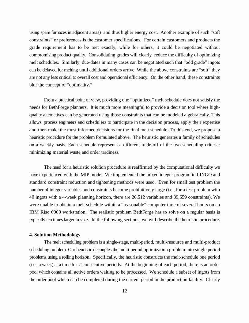
using spare furnaces in adjacent areas) and thus higher energy cost. Another example of such “soft

constraints” or preferences is the customer specifications. For certain customers and products the

grade requirement has to be met exactly, while for others, it could be negotiated without

compromising product quality. Consolidating grades will clearly reduce the difficulty of optimizing

melt schedules. Similarly, due-dates in many cases can be negotiated such that “odd grade” ingots

can be delayed for melting until additional orders arrive. While the above constraints are “soft” they

are not any less critical to overall cost and operational efficiency. On the other hand, these constraints

blur the concept of “optimality.”

From a practical point of view, providing one “optimized” melt schedule does not satisfy the

needs for BethForge planners. It is much more meaningful to provide a decision tool where high-

quality alternatives can be generated using those constraints that can be modeled algebraically. This

allows process engineers and schedulers to participate in the decision process, apply their expertise

and then make the most informed decisions for the final melt schedule. To this end, we propose a

heuristic procedure for the problem formulated above. The heuristic generates a family of schedules

on a weekly basis. Each schedule represents a different trade-off of the two scheduling criteria:

minimizing material waste and order tardiness.

The need for a heuristic solution procedure is reaffirmed by the computational difficulty we

have experienced with the MIP model. We implemented the mixed integer program in LINGO and

standard constraint reduction and tightening methods were used. Even for small test problem the

number of integer variables and constraints become prohibitively large (i.e., for a test problem with

40 ingots with a 4-week planning horizon, there are 20,512 variables and 39,659 constraints). We

were unable to obtain a melt schedule within a “reasonable” computer time of several hours on an

IBM Risc 6000 workstation. The realistic problem BethForge has to solve on a regular basis is

typically ten times larger in size. In the following sections, we will describe the heuristic procedure.

4. Solution Methodology

The melt scheduling problem is a single-stage, multi-period, multi-resource and multi-product

scheduling problem. Our heuristic decouples the multi-period optimization problem into single period

problems using a rolling horizon. Specifically, the heuristic constructs the melt-schedule one period

(i.e., a week) at a time for T consecutive periods. At the beginning of each period, there is an order

pool which contains all active orders waiting to be processed. We schedule a subset of ingots from

the order pool which can be completed during the current period in the production facility. Clearly

13

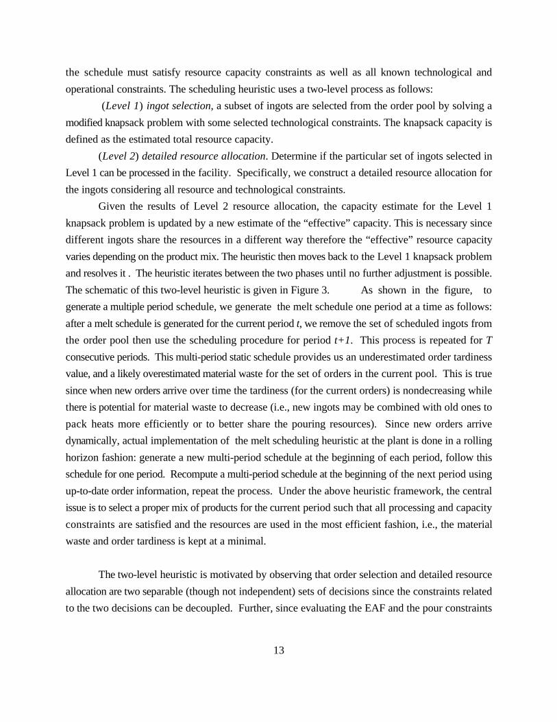
the schedule must satisfy resource capacity constraints as well as all known technological and

operational constraints. The scheduling heuristic uses a two-level process as follows:

(Level 1) ingot selection, a subset of ingots are selected from the order pool by solving a

modified knapsack problem with some selected technological constraints. The knapsack capacity is

defined as the estimated total resource capacity.

(Level 2) detailed resource allocation. Determine if the particular set of ingots selected in

Level 1 can be processed in the facility. Specifically, we construct a detailed resource allocation for

the ingots considering all resource and technological constraints.

Given the results of Level 2 resource allocation, the capacity estimate for the Level 1

knapsack problem is updated by a new estimate of the “effective” capacity. This is necessary since

different ingots share the resources in a different way therefore the “effective” resource capacity

varies depending on the product mix. The heuristic then moves back to the Level 1 knapsack problem

and resolves it . The heuristic iterates between the two phases until no further adjustment is possible.

The schematic of this two-level heuristic is given in Figure 3. As shown in the figure, to

generate a multiple period schedule, we generate the melt schedule one period at a time as follows:

after a melt schedule is generated for the current period t, we remove the set of scheduled ingots from

the order pool then use the scheduling procedure for period t+1. This process is repeated for T

consecutive periods. This multi-period static schedule provides us an underestimated order tardiness

value, and a likely overestimated material waste for the set of orders in the current pool. This is true

since when new orders arrive over time the tardiness (for the current orders) is nondecreasing while

there is potential for material waste to decrease (i.e., new ingots may be combined with old ones to

pack heats more efficiently or to better share the pouring resources). Since new orders arrive

dynamically, actual implementation of the melt scheduling heuristic at the plant is done in a rolling

horizon fashion: generate a new multi-period schedule at the beginning of each period, follow this

schedule for one period. Recompute a multi-period schedule at the beginning of the next period using

up-to-date order information, repeat the process. Under the above heuristic framework, the central

issue is to select a proper mix of products for the current period such that all processing and capacity

constraints are satisfied and the resources are used in the most efficient fashion, i.e., the material

waste and order tardiness is kept at a minimal.

The two-level heuristic is motivated by observing that order selection and detailed resource

allocation are two separable (though not independent) sets of decisions since the constraints related

to the two decisions can be decoupled. Further, since evaluating the EAF and the pour constraints

14

For periods t=1,...,T do

Step 0. Update order pool for period t: Remove ingots which have been scheduled in period1..(t-1). Add new ingots released at t. Calculate an estimated capacity of the facility, b.

Step 1. Main iterations. Iterate S times..begin

(Level 1 Iterations): Ingot Selection

Step 2. Select a set of ingots I from the order pool for period t by heuristically solving at

modified knapsack problem. The capacity of knapsack is set to the current estimate ofeffective facility capacity, b. The objective of the knapsack problem is to minimizeorder tardiness.

Step 3. Iterate the ingot selection heuristic k times using Problem Space Search1

(details are given in Figure 4 and Section 4.2)

(Level 2 Iterations): Detailed Resource Allocation

Step 4. Determine a feasible resource allocation for ingots in set I using a resourcet

allocation heuristic which packs the heats according to the EAF constraints andconfigures the pouring resources according to the pouring constraints. The objective isto minimize material waste as a result of resource allocation.

Step 5. Iterate the resource allocation heuristic k times using Problem Space Search2

(details are given in Figure 5 and Section 4.4).

Step 6. Evaluate the resource allocation in step 4. If all ingots in I are processed,t

calculate the capacity slack from all resources. Otherwise, calculate the shortfall ofcapacity b.

(Adaptive Feedback and Termination Check)

Step 7. Adjust the knapsack capacity b: if there is a capacity slack, increase b. If thereis a capacity shortfall, decrease b. If the above adjustment has changed sign during thelast two iterations, set t7t+1 and return to Step 0. Otherwise, return to Step 1 withnew capacity b. (details are given in Section 4.5)

end;enddo;

Figure 3. A Schematic Overview of the Melt Scheduling Heuristic

jNk'1 Wtk xk # b (18)

15

contributes to a majority of the computation effort, decoupling the two set of decisions tends to

reduce the computation time significantly. In the following sections we provide more detail on the

decoupling of the melt scheduling decisions into the two separate levels.

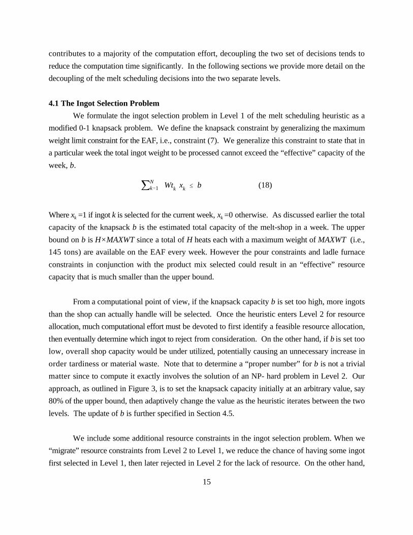
4.1 The Ingot Selection Problem

We formulate the ingot selection problem in Level 1 of the melt scheduling heuristic as a

modified 0-1 knapsack problem. We define the knapsack constraint by generalizing the maximum

weight limit constraint for the EAF, i.e., constraint (7). We generalize this constraint to state that in

a particular week the total ingot weight to be processed cannot exceed the “effective” capacity of the

week, b.

Where x =1 if ingot k is selected for the current week, x =0 otherwise. As discussed earlier the totalk k

capacity of the knapsack b is the estimated total capacity of the melt-shop in a week. The upper

bound on b is H×MAXWT since a total of H heats each with a maximum weight of MAXWT (i.e.,

145 tons) are available on the EAF every week. However the pour constraints and ladle furnace

constraints in conjunction with the product mix selected could result in an “effective” resource

capacity that is much smaller than the upper bound.

From a computational point of view, if the knapsack capacity b is set too high, more ingots

than the shop can actually handle will be selected. Once the heuristic enters Level 2 for resource

allocation, much computational effort must be devoted to first identify a feasible resource allocation,

then eventually determine which ingot to reject from consideration. On the other hand, if b is set too

low, overall shop capacity would be under utilized, potentially causing an unnecessary increase in

order tardiness or material waste. Note that to determine a “proper number” for b is not a trivial

matter since to compute it exactly involves the solution of an NP- hard problem in Level 2. Our

approach, as outlined in Figure 3, is to set the knapsack capacity initially at an arbitrary value, say

80% of the upper bound, then adaptively change the value as the heuristic iterates between the two

levels. The update of b is further specified in Section 4.5.

We include some additional resource constraints in the ingot selection problem. When we

“migrate” resource constraints from Level 2 to Level 1, we reduce the chance of having some ingot

first selected in Level 1, then later rejected in Level 2 for the lack of resource. On the other hand,

jNk'1 xk MDk,p

# Cp œ p (19)

*km =1 if Gk … Gm and xk'xm'1

0 Otherwiseœ k,m0It ,k…m

(20)

jNk'1 jN

m'1 *km # H

(21)

Minimize jNk'1 Max{0,(fk&ddk)} (22)

s.t.

fk =t if xk'1

T/2 Otherwiseœ k (23)

Constraints (18)&(21)

16

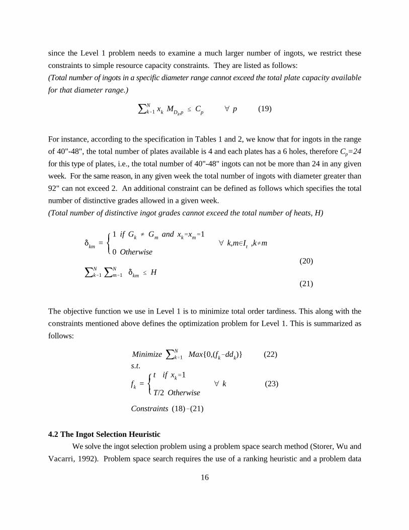
since the Level 1 problem needs to examine a much larger number of ingots, we restrict these

constraints to simple resource capacity constraints. They are listed as follows:

(Total number of ingots in a specific diameter range cannot exceed the total plate capacity available

for that diameter range.)

For instance, according to the specification in Tables 1 and 2, we know that for ingots in the range

of 40"-48", the total number of plates available is 4 and each plates has a 6 holes, therefore C =24p

for this type of plates, i.e., the total number of 40"-48" ingots can not be more than 24 in any given

week. For the same reason, in any given week the total number of ingots with diameter greater than

92" can not exceed 2. An additional constraint can be defined as follows which specifies the total

number of distinctive grades allowed in a given week.

(Total number of distinctive ingot grades cannot exceed the total number of heats, H)

The objective function we use in Level 1 is to minimize total order tardiness. This along with the

constraints mentioned above defines the optimization problem for Level 1. This is summarized as

follows:

4.2 The Ingot Selection Heuristic

We solve the ingot selection problem using a problem space search method (Storer, Wu and

Vacarri, 1992). Problem space search requires the use of a ranking heuristic and a problem data

Dk'(ddk)p1(Wtk)

p2

17

Procedure Ingot Selection

Step 0. Initialize the set of ingot selected I 7` and performance measure v 70t* *

Repeat k times.... 1

begin;Step 1. Set I7` . If ingot f must be made (“frozen”) in current period, set dd 7 Min {dd }. t f k k

Step 2. For each ingot k in the order pool, compute a desirability index based on its due datedd and weight Wt as follows: k k

Step 3. Sort the ingots in the order pool in ascending order of D , index the ordered ingots k

by [i], i.e., D # D # ...# D[1] [2] [N].

For [i] = 1 to N do

Step 4. If ingots in set I c {[i]} collectively satisfy constraints (18)-(21), then set t

I 7I c {[i]}. t t

Step 5. If the total weight of ingots currently in I exceed the knapsack capacity b, t

then go to Step 6

enddo; Step 6. Compute the objective value for current ingot selection v(I ) using (22) and (23). If t

v(I )<v , then set v 7v(I ), set I 7It t t t.* * *

Step 7. For each ingot in the order pool, perturb the due date dd as follows:k

dd 7 dd + Uniform [-u, u ], (u is a user defined parameter) go to Step 1.k k

end;

Figure 4. The Ingot Selection Heuristic based on Problem Space Search

vector. The search neighborhood is generated by first perturbing the problem data vector, applying

the ranking heuristic to the perturbed vector which establishes a new ranking, then derive a new

solution from the ranking using original problem data. In the case of the ingot selection heuristic, the

problem data vector is defined by ingot due-dates. The base ranking heuristic selects the ingots

according to a desirability index computed from the (perturbed) due-date and weight. The heuristic

then searches in this neighborhood of problem perturbation for better solutions. Details of this

procedure are summarized in Figure 4.

Minimize jHh'1 Wsth (24)

s.t.Constraints (2)',(4)',(6)'&(17)'.

18

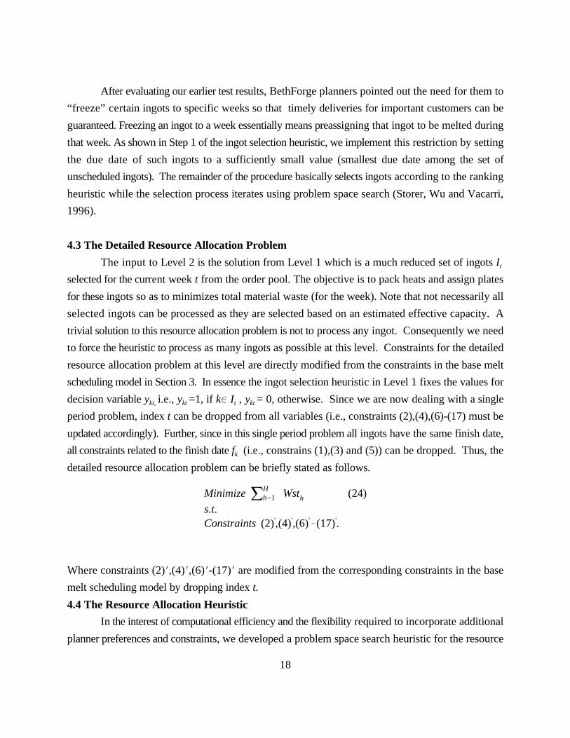
After evaluating our earlier test results, BethForge planners pointed out the need for them to

“freeze” certain ingots to specific weeks so that timely deliveries for important customers can be

guaranteed. Freezing an ingot to a week essentially means preassigning that ingot to be melted during

that week. As shown in Step 1 of the ingot selection heuristic, we implement this restriction by setting

the due date of such ingots to a sufficiently small value (smallest due date among the set of

unscheduled ingots). The remainder of the procedure basically selects ingots according to the ranking

heuristic while the selection process iterates using problem space search (Storer, Wu and Vacarri,

1996).

4.3 The Detailed Resource Allocation Problem

The input to Level 2 is the solution from Level 1 which is a much reduced set of ingots It

selected for the current week t from the order pool. The objective is to pack heats and assign plates

for these ingots so as to minimizes total material waste (for the week). Note that not necessarily all

selected ingots can be processed as they are selected based on an estimated effective capacity. A

trivial solution to this resource allocation problem is not to process any ingot. Consequently we need

to force the heuristic to process as many ingots as possible at this level. Constraints for the detailed

resource allocation problem at this level are directly modified from the constraints in the base melt

scheduling model in Section 3. In essence the ingot selection heuristic in Level 1 fixes the values for

decision variable y i.e., y =1, if k0 I , y = 0, otherwise. Since we are now dealing with a singlekt, kt t kt

period problem, index t can be dropped from all variables (i.e., constraints (2),(4),(6)-(17) must be

updated accordingly). Further, since in this single period problem all ingots have the same finish date,

all constraints related to the finish date f (i.e., constrains (1),(3) and (5)) can be dropped. Thus, thek

detailed resource allocation problem can be briefly stated as follows.

Where constraints (2)N,(4)N,(6)N-(17)N are modified from the corresponding constraints in the base

melt scheduling model by dropping index t.

4.4 The Resource Allocation Heuristic

In the interest of computational efficiency and the flexibility required to incorporate additional

planner preferences and constraints, we developed a problem space search heuristic for the resource

19

allocation problem. As described in Sections 2.2 and 2.3, decisions involved in the resource

allocation problem can be split into two basic categories: heat packing subject to EAF constraints and

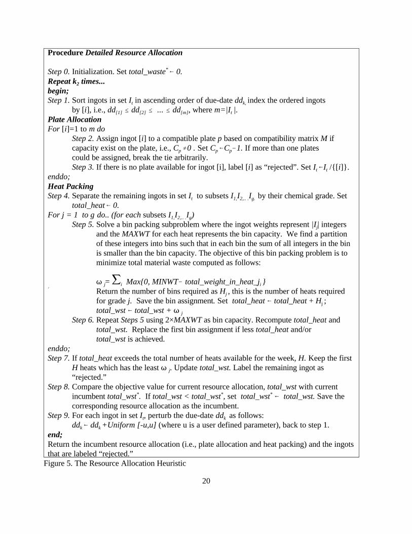
plate allocation. As shown in Figure 5, we divide the resource allocation procedure accordingly to

plate allocation and heat packing.

Although in the actual process heats are first formed in EAF then poured into ingot molds on

the plate, in the heuristic we first make sure plate resources are available before forming heats. This

is due to insights from the BethForge scheduler that the plates are typically the scarce resource.

Hence checking the plate constraints first brings us faster toward a feasible set of ingots. Plate

allocation uses a simple policy where ingots selected from Level 1 (i.e.,set I ) are first sorted by theirt

due-dates, then assigned their plate resources according to this order. The compatibility between

ingots and plates are specified by matrix M derived from information in tables 1 and 2. Since the

ingots are ordered by due date, the ingots “rejected” will have the latest due dates among ingots

competing for the same resources. Clearly, the strict due-date based priority scheme is not always

optimal. The heuristic later perturbs the due-dates (in Step 9) in an effort to alternate the priority,

thereby examining alternate resource allocations.

In the heat packing steps (Steps 4-7) ingots are packed into EAF heats. Since only one

chemical grade is allowed in each heat, ingots of different grades do not share melt resources (EAF)

at any given time. We therefore separate ingots of different grades and treat each grade group as an

independent heat packing problem. As shown in Step 5 we solve a bin packing subproblem where

each heat is a bin. We use the well known “First Fit” algorithm for this problem as follows: taking

ingots in their due-date order established by index [i], place each ingot in the first bin with enough

capacity to accommodate it. Recall that we could combine two consecutive heats to melt ingots

(constraints (6) and (8)). This is done in Step 6 where we resolve the bin-packing problem to see if

combining heats (i.e., using bin capacity of 2×MAXWT) would reduce material waste. The reason

we do not start with considering two heats at a time is that combining heats requires higher energy

consumption, and therefore is less desirable. Similar to plate allocation, alternative heat packing

solutions will be examined when the due-dates of ingots are perturbed in step 9.

The plate allocation and heat packing procedures are repeated k times, each time a slightly2

perturbed priority is used in the procedure. At the end of the k iterations, the heuristic returns the2

best resource allocation found and the ingots that are rejected. Recall that the ingot set I at Levelt

2 is the output of the ingot selection in Level 1 where an estimated effect capacity was used.

20

Procedure Detailed Resource Allocation

Step 0. Initialization. Set total_waste 7 0.*

Repeat k times...2

begin;Step 1. Sort ingots in set I in ascending order of due-date dd index the ordered ingots t k,

by [i], i.e., dd # dd # ... # dd , where m=|I |. [1] [2] [m] t

Plate AllocationFor [i]=1 to m do

Step 2. Assign ingot [i] to a compatible plate p based on compatibility matrix M if capacity exist on the plate, i.e., C …0 . Set C 7C !1. If more than one plates p p p

could be assigned, break the tie arbitrarily. Step 3. If there is no plate available for ingot [i], label [i] as “rejected”. Set I 7I /{[i]}. t t

enddo;Heat Packing Step 4. Separate the remaining ingots in set I to subsets I I I by their chemical grade. Set t 1, 2,.. . g.

total_heat7 0.

For j = 1 to g do.. (for each subsets I I I ) 1, 2,.. . g

Step 5. Solve a bin packing subproblem where the ingot weights represent |I | integers j

and the MAXWT for each heat represents the bin capacity. We find a partitionof these integers into bins such that in each bin the sum of all integers in the binis smaller than the bin capacity. The objective of this bin packing problem is tominimize total material waste computed as follows:

T = j Max{0, MINWT! total_weight_in_heat_j }j i i

Return the number of bins required as H , this is the number of heats required Nj

for grade j. Save the bin assignment. Set total_heat 7 total_heat + H ; j

total_wst 7 total_wst + T jStep 6. Repeat Steps 5 using 2×MAXWT as bin capacity. Recompute total_heat and

total_wst. Replace the first bin assignment if less total_heat and/or total_wst is achieved.

enddo;Step 7. If total_heat exceeds the total number of heats available for the week, H. Keep the first

H heats which has the least T . Update total_wst. Label the remaining ingot asj

“rejected.” Step 8. Compare the objective value for current resource allocation, total_wst with current

incumbent total_wst . If total_wst < total_wst , set total_wst 7 total_wst. Save the* * *

corresponding resource allocation as the incumbent. Step 9. For each ingot in set I , perturb the due-date dd as follows:t k

dd 7 dd +Uniform [-u,u] (where u is a user defined parameter), back to step 1.k k

end; Return the incumbent resource allocation (i.e., plate allocation and heat packing) and the ingotsthat are labeled “rejected.”

Figure 5. The Resource Allocation Heuristic

21

An overestimation of capacity or a skewed product mix could both result in one or more of the ingots

being rejected in the plate allocation and/or heat packing steps. The two functions are linked by the

zero WIP constraint: whatever is melted must be poured, and by the same token, if a certain ingot

cannot be poured, it must not be melted. From the viewpoint of algorithm design, we could perform

heat packing and plate allocation in a reversed sequence. However, after testing several case

problems using real data we found that the plate allocation constraints are, in most of the cases, the

binding constraints. Hence in our implementation we first allocate the plate resources then consider

the heat packing function.

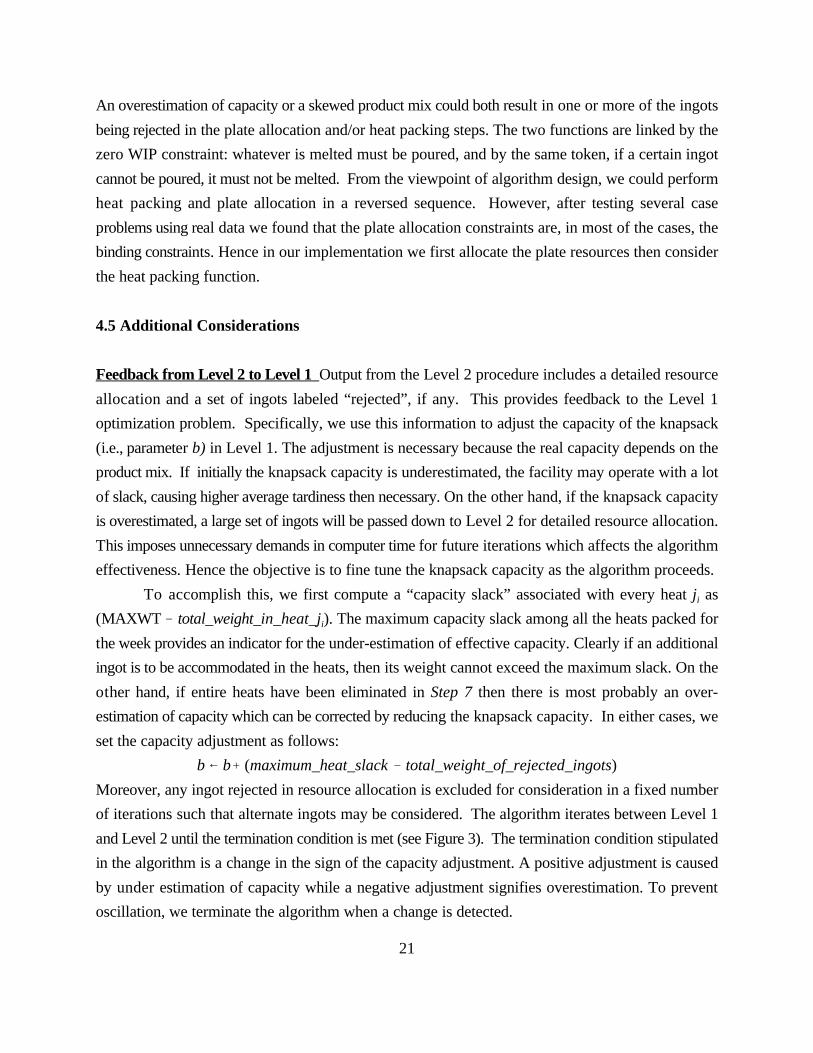
4.5 Additional Considerations

Feedback from Level 2 to Level 1 Output from the Level 2 procedure includes a detailed resource

allocation and a set of ingots labeled “rejected”, if any. This provides feedback to the Level 1

optimization problem. Specifically, we use this information to adjust the capacity of the knapsack

(i.e., parameter b) in Level 1. The adjustment is necessary because the real capacity depends on the

product mix. If initially the knapsack capacity is underestimated, the facility may operate with a lot

of slack, causing higher average tardiness then necessary. On the other hand, if the knapsack capacity

is overestimated, a large set of ingots will be passed down to Level 2 for detailed resource allocation.

This imposes unnecessary demands in computer time for future iterations which affects the algorithm

effectiveness. Hence the objective is to fine tune the knapsack capacity as the algorithm proceeds.

To accomplish this, we first compute a “capacity slack” associated with every heat j asi

(MAXWT ! total_weight_in_heat_j ). The maximum capacity slack among all the heats packed fori

the week provides an indicator for the under-estimation of effective capacity. Clearly if an additional

ingot is to be accommodated in the heats, then its weight cannot exceed the maximum slack. On the

other hand, if entire heats have been eliminated in Step 7 then there is most probably an over-

estimation of capacity which can be corrected by reducing the knapsack capacity. In either cases, we

set the capacity adjustment as follows:

b 7 b% (maximum_heat_slack & total_weight_of_rejected_ingots)

Moreover, any ingot rejected in resource allocation is excluded for consideration in a fixed number

of iterations such that alternate ingots may be considered. The algorithm iterates between Level 1

and Level 2 until the termination condition is met (see Figure 3). The termination condition stipulated

in the algorithm is a change in the sign of the capacity adjustment. A positive adjustment is caused

by under estimation of capacity while a negative adjustment signifies overestimation. To prevent

oscillation, we terminate the algorithm when a change is detected.

22

Checking for “Maximum-Allowable-Waste” Schedules After our initial testing, the BethForge

management expressed interest in seeking schedules that have little or no material waste due to the

high cost of material and energy. Clearly this requirement could affect the due-date performance.

A possible strategy is to delay the melting of “high waste” ingots hoping that either additional orders

can be negotiated or chemical grades can be consolidated with other orders, which results in a better

configuration for resource allocation. To incorporate the “maximum allowable waste” criterion into

the heuristic, we allow the user to specify the maximum allowable waste per heat. This figure

specifies the allowable amount of waste (per heat) for a schedule to be considered feasible. Taking

this restriction to an extreme results in a “zero-waste” schedule. This is sometimes possible for at

least the first few weeks into the future. However, the impact of “zero-waste” schedule on overall

scheduling efficiency needs to be carefully examined. For instance, certain “odd-grade” ingots that

may never be combined with any other ingots tend to get pushed beyond their due dates, thus

affecting the overall due date performance. In other words, there may be a schedule which satisfies

the “maximum allowable waste” requirement for the current week but at the same time causes

unusually high tardiness for the future. We provide some computational analysis to this effect in

Section 5.

In implementing the maximum allowable waste restriction we add an additional check in the

heuristic after Step 6 which evaluates each “bin” to see if its waste conforms to the permissible limit.

If the actual waste in a bin exceeds the allowable limit, one of the ingots from that bin is labeled

“rejected” such that in the following iterations alternative ingots will be considered. Eventually, the

procedure will either find a packing that conforms to the waste limit, or fails to do so when all the

ingots of this chemical grade are rejected. However, in testing on real data, we were typically able

to find “maximum allowable waste” solution.

5. Computational Experiments and Analysis of Results

The following section describes the experimental design we used to determine the important

factors affecting the performance of the melt scheduling heuristic. Section 5.2 presents the

computational results obtained from actual order data from BethForge.

5.1 Design of Experiments

We first identified several parameters in the heuristic that need to be determined for testing

the algorithm’s performance on the available data sets. These are:

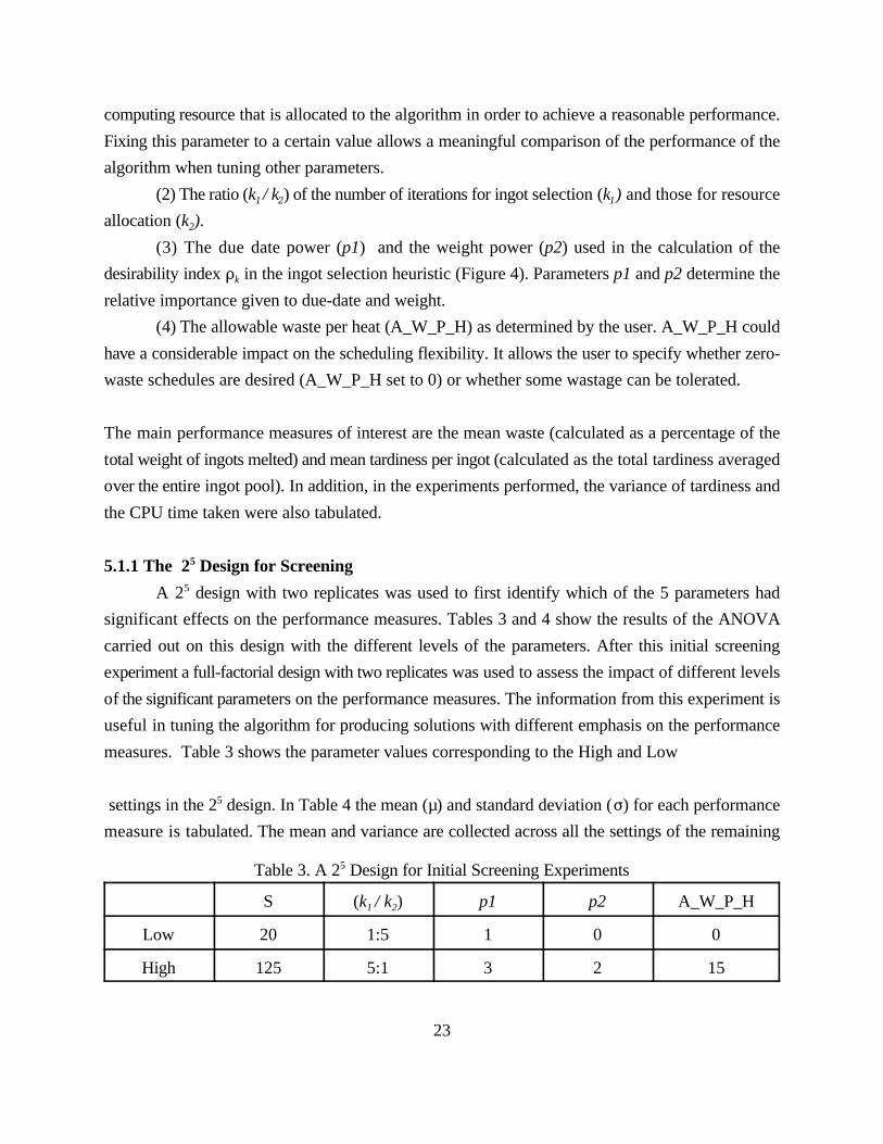
(1) The total number of main iterations (S) performed. This is a measure of the total

23

S (k / k )1 2 p1 p2 A_W_P_H

Low 20 1:5 1 0 0

High 125 5:1 3 2 15

Table 3. A 2 Design for Initial Screening Experiments5

computing resource that is allocated to the algorithm in order to achieve a reasonable performance.

Fixing this parameter to a certain value allows a meaningful comparison of the performance of the

algorithm when tuning other parameters.

(2) The ratio (k / k ) of the number of iterations for ingot selection (k ) and those for resource1 2 1

allocation (k ). 2

(3) The due date power (p1) and the weight power (p2) used in the calculation of the

desirability index D in the ingot selection heuristic (Figure 4). Parameters p1 and p2 determine thek

relative importance given to due-date and weight.

(4) The allowable waste per heat (A_W_P_H) as determined by the user. A_W_P_H could

have a considerable impact on the scheduling flexibility. It allows the user to specify whether zero-

waste schedules are desired (A_W_P_H set to 0) or whether some wastage can be tolerated.

The main performance measures of interest are the mean waste (calculated as a percentage of the

total weight of ingots melted) and mean tardiness per ingot (calculated as the total tardiness averaged

over the entire ingot pool). In addition, in the experiments performed, the variance of tardiness and

the CPU time taken were also tabulated.

5.1.1 The 2 Design for Screening5

A 2 design with two replicates was used to first identify which of the 5 parameters had5

significant effects on the performance measures. Tables 3 and 4 show the results of the ANOVA

carried out on this design with the different levels of the parameters. After this initial screening

experiment a full-factorial design with two replicates was used to assess the impact of different levels

of the significant parameters on the performance measures. The information from this experiment is

useful in tuning the algorithm for producing solutions with different emphasis on the performance

measures. Table 3 shows the parameter values corresponding to the High and Low

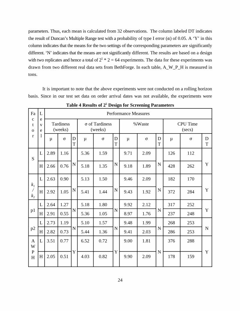
settings in the 2 design. In Table 4 the mean (µ) and standard deviation (F) for each performance5

measure is tabulated. The mean and variance are collected across all the settings of the remaining

24

Factor

Level

Performance Measures

Tardiness(weeks)

F of Tardiness(weeks)

%Waste CPU Time(secs)

µ F DT

µ F DT

µ F DT

µ F DT

SL 2.89 1.16

N

5.36 1.59

N

9.71 2.09

N

126 112

YH 2.66 0.76 5.18 1.35 9.18 1.89 428 262

k1

/k2

L 2.63 0.90

N

5.13 1.50

N

9.46 2.09

N

182 170

YH 2.92 1.05 5.41 1.44 9.43 1.92 372 284

p1L 2.64 1.27

N5.18 1.80

N9.92 2.12

N317 252

YH 2.91 0.55 5.36 1.05 8.97 1.76 237 248

p2L 2.73 1.19

N5.10 1.57

N9.48 1.99

N268 253

NH 2.82 0.73 5.44 1.36 9.41 2.03 286 253

AWPH

L 3.51 0.77

Y

6.52 0.72

Y

9.00 1.81

N

376 288

YH 2.05 0.51 4.03 0.82 9.90 2.09 178 159

Table 4 Results of 2 Design for Screening Parameters5

parameters. Thus, each mean is calculated from 32 observations. The column labeled DT indicates

the result of Duncan’s Multiple Range test with a probability of type I error (") of 0.05. A ‘Y’ in this

column indicates that the means for the two settings of the corresponding parameters are significantly

different. ‘N’ indicates that the means are not significantly different. The results are based on a design

with two replicates and hence a total of 2 * 2 = 64 experiments. The data for these experiments was5

drawn from two different real data sets from BethForge. In each table, A_W_P_H is measured in

tons.

It is important to note that the above experiments were not conducted on a rolling horizon

basis. Since in our test set data on order arrival dates was not available, the experiments were

25

performed assuming a static pool of ingots with no new order arrivals over time. It should be

understood that the flexibility and full potential of the algorithm are constrained by this restriction.

In the actual scheduling procedure we implemented for BethForge, new orders are added to the pool

in a periodic basis.

The following conclusions can be drawn from Table 4. Only parameter A_W_P_H has a

significant effect on the average tardiness. A_W_P_H affects the flexibility available in scheduling the

ingots. Setting A_W_P_H to zero leaves no room for trading off waste in favor of tardy ingots. Odd

grade ingots tend to get pushed back whenever alternate “zero-waste” schedules can be found. The

interaction between p1 and A_W_P_H was also found to be significant for average tardiness. Since

p1 controls the relative importance of due date in the desirability index, it is natural to expect p1 to

have some influence on the average tardiness. Likewise, the variance of tardiness for a given pool of

ingots (calculated based on the tardiness values of each ingot in the pool) is affected only by

A_W_P_H.

The computational time, as expected, depends on the total number of main iterations (S) and

also on how the computation effort is divided between the two levels of the algorithm (k /k ). As in1 2

the case of tardiness, the CPU time depends on both p1 and A_W_P_H. Both these factors affect

directly the flexibility allowed in scheduling ingots. As scheduling flexibility reduces, one would

expect a longer computation times for schedule generation.

5.1.2 The Full Factorial Design

Based on an analysis of the 2 experiments, a full factorial experiment was designed to test5

the effects of various settings of the parameters p1 and A_W_P_H which were found to be significant

factors affecting the two primary performance measures viz. tardiness and waste. The other factors

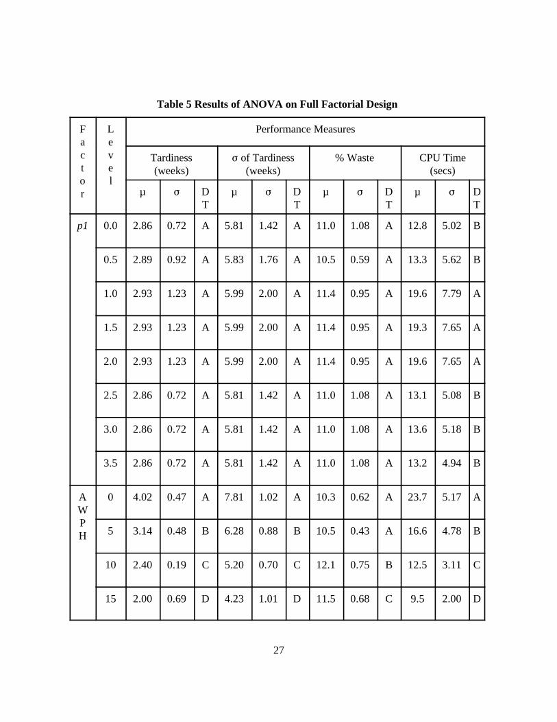
were set to levels best suited for minimizing the CPU time. Tables 5 summarizes the results of the

ANOVA.

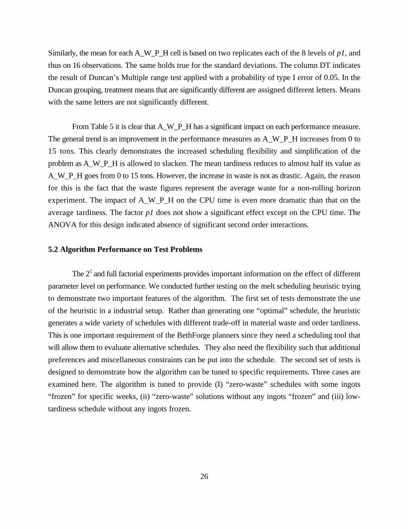
In the full factorial experiment, 8 levels of p1 were investigated, each for 4 levels of

A_W_P_H. Again, two replicates were used and this gave rise to 8 * 4 * 2 = 64 experiments. The

experiments were conducted based on real order data from BethForge. As before, Table 5 shows

mean and standard deviation of average job tardiness, the standard deviation of tardiness, the average

percentage waste and the CPU time. The mean for each cell for the factor p1 is calculated across the

4 levels of A_W_P_H. With two replicates for each A_W_P_H level, this gives 8 observations.

26

Similarly, the mean for each A_W_P_H cell is based on two replicates each of the 8 levels of p1, and

thus on 16 observations. The same holds true for the standard deviations. The column DT indicates

the result of Duncan’s Multiple range test applied with a probability of type I error of 0.05. In the

Duncan grouping, treatment means that are significantly different are assigned different letters. Means

with the same letters are not significantly different.

From Table 5 it is clear that A_W_P_H has a significant impact on each performance measure.

The general trend is an improvement in the performance measures as A_W_P_H increases from 0 to

15 tons. This clearly demonstrates the increased scheduling flexibility and simplification of the

problem as A_W_P_H is allowed to slacken. The mean tardiness reduces to almost half its value as

A_W_P_H goes from 0 to 15 tons. However, the increase in waste is not as drastic. Again, the reason

for this is the fact that the waste figures represent the average waste for a non-rolling horizon

experiment. The impact of A_W_P_H on the CPU time is even more dramatic than that on the

average tardiness. The factor p1 does not show a significant effect except on the CPU time. The

ANOVA for this design indicated absence of significant second order interactions.

5.2 Algorithm Performance on Test Problems

The 2 and full factorial experiments provides important information on the effect of different5

parameter level on performance. We conducted further testing on the melt scheduling heuristic trying

to demonstrate two important features of the algorithm. The first set of tests demonstrate the use

of the heuristic in a industrial setup. Rather than generating one “optimal” schedule, the heuristic

generates a wide variety of schedules with different trade-off in material waste and order tardiness.

This is one important requirement of the BethForge planners since they need a scheduling tool that

will allow them to evaluate alternative schedules. They also need the flexibility such that additional

preferences and miscellaneous constraints can be put into the schedule. The second set of tests is

designed to demonstrate how the algorithm can be tuned to specific requirements. Three cases are

examined here. The algorithm is tuned to provide (I) “zero-waste” schedules with some ingots

“frozen” for specific weeks, (ii) “zero-waste” solutions without any ingots “frozen” and (iii) low-

tardiness schedule without any ingots frozen.

27

Factor

Level

Performance Measures

Tardiness(weeks)

F of Tardiness(weeks)

% Waste CPU Time(secs)

µ F DT

µ F DT

µ F DT

µ F DT

p1 0.0 2.86 0.72 A 5.81 1.42 A 11.0 1.08 A 12.8 5.02 B

0.5 2.89 0.92 A 5.83 1.76 A 10.5 0.59 A 13.3 5.62 B

1.0 2.93 1.23 A 5.99 2.00 A 11.4 0.95 A 19.6 7.79 A

1.5 2.93 1.23 A 5.99 2.00 A 11.4 0.95 A 19.3 7.65 A

2.0 2.93 1.23 A 5.99 2.00 A 11.4 0.95 A 19.6 7.65 A

2.5 2.86 0.72 A 5.81 1.42 A 11.0 1.08 A 13.1 5.08 B

3.0 2.86 0.72 A 5.81 1.42 A 11.0 1.08 A 13.6 5.18 B

3.5 2.86 0.72 A 5.81 1.42 A 11.0 1.08 A 13.2 4.94 B

AWPH

0 4.02 0.47 A 7.81 1.02 A 10.3 0.62 A 23.7 5.17 A

5 3.14 0.48 B 6.28 0.88 B 10.5 0.43 A 16.6 4.78 B

10 2.40 0.19 C 5.20 0.70 C 12.1 0.75 B 12.5 3.11 C

15 2.00 0.69 D 4.23 1.01 D 11.5 0.68 C 9.5 2.00 D

Table 5 Results of ANOVA on Full Factorial Design

28

The tests have been carried out on three sets of order data from BethForge. These data sets are

different from the ones used for the parameter tuning experiments. The results of these tests are

shown graphically in Figures 8 through 13. The following sections discuss these results in detail.

5.2.1 Bi-criterion Plots

Figures 6 through 8 each show two representative bi-criterion plots. The plots are generated

by keeping track of the feasible schedules generated by the problem space search. Here the waste is

represented in tons and the mean tardiness in weeks. These plots visually demonstrate the trade-off

between the two objectives. An efficient frontier of non-dominated solutions can be observed in lower

left of each plot. The efficient frontier suggests an obvious tradeoff between waste and tardiness. In

actual implementation, a population of schedules as shown in the Figure can be generated for all

future weeks on a periodic basis. The planner will be able to click on a particular data point on the

graph and review the actual melt schedule associated with that point. This will include all the ingots

selected for the week and detailed resource allocation. The planner can than contemplate additional

factors such as energy consumption and labor availability which are not included in the original

model. It will be straight forward for the planner to either select schedules out of the population, or

alter part of an existing schedule, then reschedule.

5.2.2 Bar Graphs

Figures 9 through 11 show three bar graphs for each of the test data sets. These graphs plot

the average waste (in tons) and the average tardiness per ingot (in weeks) for each week. The three

graphs for each data set illustrate how the algorithm can be tuned to specific planning requirements

and how the algorithm performs over time. The first graph in each set shows the cases where some

ingots are “frozen” a priori for particular weeks while the emphasis is on generating zero-waste

schedules. The second graph shows the same setup except that the restriction on freezing ingots is

removed. The third graph shows the cases where the heuristic emphasizes only on shipping

performance (low tardiness), without using the zero-waste policy and no restriction on frozen ingots.

As discussed earlier, due-date setting could have a profound impact on overall scheduling

performance. In this case, “frozen” ingots represent internal due-date set by marketing and sales for

the purpose of guaranteeing shipping performance for a certain customers. As we move from the first

to the second graph in each figure, the scheduling flexibility increases since now none of the ingots

are required to be frozen in any week. This allows the algorithm to search a larger solution space and

29

consequently results in better waste figures. From the graphs it should be clear that while these

artificial due-dates indeed improves the shipping performance since tardiness is generally lower, they

have a significant impact on the amount of waste produced. Similarly, from the third graphs of

Figures 9-11 it is clear that as the emphasis shifts to shipping performance (low tardiness), the waste

figures increase rather significantly.

Several important inferences can be drawn from these graphs. First, it demonstrates that the

interest of customer satisfaction (shipping performance) from a marketing and sales perspective could

unintentionally impose a hefty cost (waste) on manufacturing. Second, while the graphs in Figures

9-11 are generated by a rolling horizon schedule, due to the amount of test data available to us, the

order pool information is not updated, i.e., the melt schedules are generated, one week at a time, from

a static order pool. This explains partially the high waste figures towards the end weeks: once most

of the ingots have been scheduled, there is little flexibility available to schedule the few remaining

ingots. Hence waste reduction becomes increasingly difficult as one progresses through the weeks.

When the order pool information is update more frequently, there is a chance that new orders arrive

over time will match with the odd-grade, odd-size orders and reduce the overall waste figure. We

did limited testing on this conjecture using the setting of low tardiness without frozen ingots: suppose

the original planning horizon is T, the original order pool is based on visibility at week 0 for T weeks,

we obtained additional order pool views from week (1/3)T, and week (2/3)T onward. Thus, in data

set 1 where we have a planning horizon of 51 weeks, we obtained a refreshed order pool view at

weeks 17 and at week 34, this in term affects the melt schedules generated from weeks 17 and 34

onward. To test the order-matching conjecture we consider only those orders that can be matched

with waste-producing orders (ones having the same chemical grade). The test results are given in

Figure 12. As shown in the three graphs corresponding to the three data sets, the overall waste figure

indeed reduced somewhat when compared to Figures 9-11, although the waste figures toward the

end-weeks remain higher. After further examination it becomes clear that although the increased

order pool provide some opportunity for reducing the wastes, some odd-size ingots simply can not

be matched in a melt. The heuristic tends to delay scheduling these ingots till the last minute when

the tardiness measure takes into effect. This result implies that it is beneficial to consolidate chemical

grades among ingots and it may be necessary to adjust the pricing for odd-size ingots to compensate

for the enormous manufacturing costs incurred.

6. Implementation Experience and Conclusions

30

The above model and solution heuristic provide a foundation for a practical melt scheduling

tool. We implemented and installed the melt scheduling tool at BethForge in 1997. In our

implementation we first coded the melt scheduling heuristic as a stand-alone routine in C++ for

Pentium PC’s. To introduce the melt scheduling procedure as a day-to-day decision tool fully

integrated with existing BethForge systems we built a flexible user interface for the scheduler to

incorporate his input. Moreover, in order to retrieve up-to-date order information, ingot

specifications and other engineering details we built a software interface with their enterprise

information system. Fortunately most BethForge planners are proficient spreadsheet users so we

were able to use Lotus spreadsheet as a template which integrates ad hoc user input, links to the

information system, and the melt scheduling algorithm. We implemented the spreadsheet template

using standard macro functions, while the enterprise system interface was built using host control

language called Powerhouse. A user may retrieve current order data (or order forecast) along with

related engineering information, make changes and adjustments to input parameters, run the melt

scheduling algorithm, then view the output in graphs and statistical tables. Then, the user may choose

to make further changes to input parameters and rerun the scheduling algorithm, to “freeze” a certain

part of the schedule and rerun the scheduling algorithm, or to pick a particular melt schedule and

make minor changes according to his special considerations.

We developed an efficient melt scheduling heuristic for the steel manufacturing process.

However, to the BethForge management, the real value of our implementation are insights gained

from test results and graphic tools such as the ones presented in sections 5.2.1 and 5.2.2. These

results bring out the interesting tradeoff between the business objective (shipping performance) and

the manufacturing objective (waste reduction). The bi-criterion graphs visually demonstrate this

tradeoff. From a managerial viewpoint, identifying this tradeoff has significant value since it not only

helps melt scheduling, but it helps the planner to explore and evaluate non-scheduling alternatives.

For instance, in practice there are different ways a process engineer could reduce the impact of

material waste. For some chemical grades, it is possible to dump the left-over material into a heated

ladle, adjust its chemical composition and save for later use. It is possible to use the trade-off

information and negotiate a more “schedule-friendly” material grade or other order specifications with

their customers. This information is also useful in consolidating multiple grades, combining future

orders at a discount price (so as to reduce material waste), or to suggest more flexible equipment

configurations for the melting operations.

The melt scheduling algorithm developed in this paper provides a decision tool, not to identify

31

one “optimal” schedule, but to examine a large number of alternate schedules for the weekly melt

scheduling problem. This tool is especially helpful when equipment failures or other unforseen events

require frequent rescheduling of the melt facility. It has also been useful for the melt scheduler to

generate initial schedules which he adapts using additional qualitative knowledge. The bar graphs

(section 5.2.2) generated along with the melt schedule allow the planners to examine long term effects

of current scheduling policies such as “zero-waste” scheduling or “order freezing” policies.

Acknowledgments

This research is supported in part by the National Science Foundation under Grant SBR-94-22862

and a grant from the Bethlehem Steel Corporation. We are in debt to many BethForge personnel for

their help and support throughout the project.

REFERENCES

Bagchi, Uttarayan, Julien, Fran\c cois M., and Magazine, Michael J., 1994. Due-date assignment to

multi-job customer orders, Management Science, 40 1389-1392.

Baker, Kenneth R. 1984, Sequencing rules and due-date assignments in a job shop, Management

Science, 30 1093-1104.

Bookbinder, James H. and H'ng, Bak-Tee,1986.Production lot sizing for deterministic rolling

schedules. Journal of Operations Management, 6, 349-362.

Chand, Suresh, 1983. Rolling horizon procedures for the facilities in series inventory model with

nested schedules. Management Science, 29, 237-249.

Chand, Suresh, Traub, Rodney, and Uzsoy, Reha, 1997. Rolling horizon procedures for the single

machine deterministic total completion time scheduling problem with release dates. ANOR 70, 115-

125.

Cheng, T.C.E., 1994, Optimal due-date assignment in an assembly shop, International Journal of

Operations & Production Management, 14, 31-42.

32

Cheng, T.C.E. and Gupta, M.C., 1989, Survey of scheduling research involving due date

determination decisions, European Journal of Operational Research, 38 156-166.

De, Prabuddha, Ghosh, Jay B., and Wells, Charles E., 1994, Due-date assignment and early/tardy

scheduling on identical parallel machines, Naval Research Logistics, 41 17-32.

Dellaert, Nico P., 1991, Due-date setting and production control, International Journal of

Production Economics, 23 59-67.

Doshi, Bhavin, K.S. Naphade, R.H. Storer, S.D. Wu and J. Moorkanat, “Melt Scheduling in the

Steel Industry- A Case Study at the BethForge Corporation,” in Proceedings, Industrial Engineering

Research Conference, Minneapolis, May 1996.

Dorn, Jürgen and W. Slany, 1994. A flow shop with compatibility constraints in a steelmaking plant,

in Intelligent Scheduling, M. Zweben and M. Fox (eds.), Morgan Kaufmann, San Francisco.

Duenyas, Izak 1995, Single facility due date setting with multiple customer classes, Management

Science, 41 608-619.

Luss, Hanan, and Rosenwein, Moshe B., 1993, A due date assignment algorithm for multiproduct

manufacturing facilities, European Journal of Operational Research, 65 187-198.

Minton, S., M. Johnston, A. Philips, and P. Laird, 1989. Solving large-scale constraint satisfaction

and scheduling problems using a heuristic repair method. Proceedings, the 8th National Conference

on Artificial Intelligence, AAAI press, Menlo Park, CA.

Naphade, K.S., B.H. Doshi, S.D. Wu and R.H. Storer, 1996. A local search algorithm for heavily

constrained bi-criterion scheduling problems. Proceedings, Industrial Engineering Research

Conference, Minneapolis.

Numao, M., S. Morishita, 1989. A scheduling environment for steel-making processes. Proceedings,

5th International Conference on Artificial Intelligence for Industrial Applications, IEEE computer

society press, Los Alamitos, CA.

33

Ovacik, I.M., and Uzsoy, R., 1995. Rolling horizon procedures for dynamic parallel machine

scheduling with sequence-dependent setup times. International Journal of Production Research, 33,

3173-3192.

Ozdamar, Linet, and Yazgac, Tulin, 1997, Capacity driven due date setting in make-to-order

production systems, International Journal of Production Economics, 49 29-44.

Russell, R.A., and Urban, T.L., 1993. Horizon extension for rolling production schedules: Length and

accuracy requirements. International Journal of Production Economics, 29, 111-122.

Seidmann, Abraham, and Smith, Milton L.,1981, Due date assignment for production systems,

Management Science, 27 571-581.

Sethi, S. and Sorger, G., 1991. A theory of rolling horizon decision making.

Annals of Operations Research, 29, 387-416.

Stauffer, L., and Liebling, Th.M.,1997. Rolling horizon scheduling in a rolling-mill, Annals of

Operations Research, 69, 323-349.

Storer, R.H., Wu, S.D. and Vaccari, 1996. Local Search in Problem and Heuristic Space for Job

Shop Scheduling. ORSA Journal on Computing, 8.

Storer, R.H., Wu, S.D. and Vaccari, 1992. New Search Spaces for Sequencing Problems with

Application to Job Shop Scheduling. Management Science, 38 1495-1509,.

Udo, G., 1993, An investigation of due-date assignment using workload information of a dynamic

shop, International Journal of Production Economics

29 89-101.

Uzsoy, R., and Ovacik, I.M., 1994. Rolling horizon algorithms for a single-machine dynamic

scheduling problem with sequence-dependent setup times, International Journal of Production

Research 32, 1243-1263.

34

Venkataraman, R., and Smith, S.B., 1996. Disaggregation to a rolling horizon master production

schedule with minimum batch-size production restrictions International Journal of Production

Research, 34, 1517-1537.

Vig, Michelle M. and Dooley, Kevin J., 1991, Dynamic rules for due-date assignment, IJPR, 29

1361-1377.

Wein, Lawrence M., 1991, Due-date setting and priority sequencing in a multiclass M/G/1 queue,

Management Science, 37 834-850.