Melbourne Institute Working Paper Series

Working Paper No. 41/13Retirement Decisions of Couples: The Impact of Spousal Characteristics and Preferences on the Timing of Retirement

Diana Warren

Retirement Decisions of Couples: The Impact of Spousal Characteristics

and Preferences on the Timing of Retirement*

Diana Warren Melbourne Institute of Applied Economic and Social Research

The University of Melbourne

Melbourne Institute Working Paper No. 41/13

ISSN 1328-4991 (Print)

ISSN 1447-5863 (Online)

ISBN 978-0-7340-4335-1

December 2013

* This paper uses unit record data from the Household, Income and Labour Dynamics in Australia (HILDA) Survey. The HILDA Project was initiated and is funded by the Australian Government Department of Social Services (DSS) and is managed by the Melbourne Institute of Applied Economic and Social Research (Melbourne Institute). The findings and views reported in this paper, however, are those of the author and should not be attributed to either DSS or the Melbourne Institute. I thank Bruce Headey, Jeff Borland, Hielke Buddelmeyer and Barbara Hanel for their valuable comments. Contact: <dwarren@unimelb.edu.au>, Tel: +61 3 9035 5712.

Melbourne Institute of Applied Economic and Social Research

The University of Melbourne

Victoria 3010 Australia

Telephone (03) 8344 2100

Fax (03) 8344 2111

Email melb-inst@unimelb.edu.au

WWW Address http://www.melbourneinstitute.com

2

Abstract

This paper provides new evidence of coordination of retirement by mature age couples in

Australia. Two complementary estimation approaches are used to highlight the importance of

taking the household decision-making context into account when modeling the retirement

behaviour of partnered men and women. First, a single risk hazard model provides insights

into the influences of a spouse’s characteristics on the retirement decision of the individual.

Second, a competing-risks framework is used to examine the retirement behaviour of couples

exiting from a situation in which both are in paid employment. There is strong evidence of

coordination of retirement by mature age couples in Australia due to complementarities in

leisure and, for women, because of caring responsibilities. In particular, the results suggest

that women may delay their own retirement if their partner has a financial incentive to

continue in the labour force; or retire early to care for a partner who is in poor health.

JEL classification: D130, J260

Keywords: Retirement, older workers, households, leisure, complementarity

3

1. Introduction

As a growing number of women approach old age with substantial work histories, the topic of

couples’ retirement is becoming increasingly important. Because of the need to balance the

preferences and constraints of both partners, decisions about retirement in couple households are

likely to be made jointly, rather than by the individuals alone. The decision about whether one or both

members of a couple should leave the labour force depends on many factors, including preferences for

joint leisure time, work-limiting health conditions, caring responsibilities, pension eligibility and the

resulting change in household income if one or both members of the couple are no longer in paid

employment.

The prevalence of joint retirement among couples has important implications for retirement policy, as

any policy that increases the incentive for one member of a couple to leave the labour force is likely to

have additional ‘spillover’ effects on the labour force participation of their spouse. For example,

policies which encourage individuals to delay their retirement, such as the gradual increasing of the

qualifying age for the Age Pension, may have a twofold effect in couple households if the result is

that both members of a couple delay their retirement due to a preference for leisure time spent

together. On the other hand, policies such as the abolition of tax on superannuation taken after the age

of 60 may create an incentive for both members of a couple to retire early, particularly if the resulting

increase in superannuation wealth allows them to achieve their target level of retirement savings

sooner than they otherwise would have. Therefore, the inclusion of spousal characteristics in the

analysis of the retirement decisions of partnered men and women is important, as it enables the

significance of cross-spousal effects to be determined. If these effects are important, modeling the

retirement behaviour of partnered men and women without considering the characteristics and

preferences of their partner may lead to errors in predicting the impact of a change in Social Security

policy on retirement behaviour (Deschryvere, 2005).

This paper provides new evidence of coordination of retirement by mature age couples in Australia,

and is the first to incorporate measures of relationship satisfaction, decision making power in the

household, and financial incentives faced by both members of the couple and into models of

retirement decisions in couple households. Two complementary estimation approaches are used to

demonstrate the importance of taking the household decision-making context into account when

modeling the retirement behaviour of partnered men and women. First, a single risk hazard model

provides insights into the influences of a spouse’s characteristics on the retirement decision of the

individual. Second, a competing-risks framework is used to examine the retirement behaviour of

couples exiting from a situation in which both are in paid employment.

There is strong evidence of coordination of retirement among Australian couples, with over 20% of

retired individuals who were living with a spouse or partner at the time of their retirement

4

coordinating their retirement with their spouse. This coordination of retirement is due to

complementarities in leisure and, for women, because of caring responsibilities. In particular, the

results suggest that women may delay their own retirement if their partner has a financial incentive to

continue in the labour force; or retire early to care for a partner who is in poor health.

The remainder of this paper is organised as follows. Section 2 gives a brief overview of the existing

literature on retirement decisions in couple households. Section 3 describes data from the Household,

Income and Labour Dynamics in Australia (HILDA) survey and outlines the econometric analysis.

The results of the analysis are presented in section 4 and section 5 concludes.

2. Previous Studies of Retirement Decisions in Couple Households

While most studies of the retirement process have concentrated on the retirement behaviour of

individuals, and particularly of men, much less is known about the joint labour force behaviour of

older couples. However, with the increase in labour force participation of older women, attention is

shifting towards the issue of the labour supply of older couples. A growing body of literature suggests

that joint retirement among couples is relatively common. In the United States, Hurd (1990), Gustman

and Steinmeier (1994 and 2000), Blau (1998), Smith and Moen (1998) and Coile (2004) using data

from the United States New Beneficiary Survey (NBS), the National Longitudinal Survey of Mature

Women (NLS), the Retirement History Survey (RHS), the Cornell Retirement and Well Being Study

and the Health and Retirement Study (HRS) respectively, all find evidence of coordinated retirement

among couples. For example, Hurd (1990) finds that in couples where both the husband and the wife

retired after the age of 54, 25% retired within one year of their spouse. Evidence of couples

coordinating the timing of their retirement has also been found for Germany (Blau and Riphahn,

1999), Austria (Zweimuller et al., 1996), Denmark (An, Christensen and Datta Gupta, 2004), Brazil

(Queiroz, 2006), Canada (Baker, 1999) and the United Kingdom (Schirle, 2008).

Four main hypotheses have been put forward to explain the tendency of couples to retire at around the

same time. The most common explanation for joint retirement is the ‘complementarities in leisure’

hypothesis. That is, many people have a preference to spend leisure time in retirement with their

spouse rather than retiring alone, and therefore couples choose to retire at around the same time.

Another explanation for couples coordinating their retirement is that of ‘assortative mating’. This

theory describes the fact that individuals tend to choose a partner who shares similar preferences

about work and leisure, and due to this similarity in preferences, the timing of their retirement

coincides (Deschryvere, 2005). Poor health or chronic illness may influence individual retirement, and

may also increase the necessity of care-giving, thereby influencing the spouse’s retirement behaviour

(Jimenez-Martin and Labeaga, 1999). Another, less commonly accepted, explanation for joint

retirement is that economic factors affecting both members of the couple cause a positive correlation

between retirement dates.

5

Several methods have been used to examine the retirement behaviour of couples. For example, Hurd

(1990), Gustman and Steinmeier (2000 and 2002) and Maestas (2001) assume that household

preferences are given by a household utility function and estimate structural models of joint

retirement. Blau (1998), Blau and Riphahn (1999), Jimenez-Martin and Labeaga (1999) and

Zweimuller et al. (1996) use multinomial logistic models to explain the joint labour market states of

husbands and wives. Johnson and Favreault (2001), Michaud (2003) and Coile (2004) estimate

reduced form models exploring the cross-effects of one spouse’s characteristics on the retirement

decision of the other spouse. An, Christensen and Datta Gupta (2004) and Pozzoli and Ranzani (2009)

analyse the joint distribution of the durations until retirement for husbands and wives.

2.1 Preferences for Joint Leisure Time

Regardless of the empirical strategy used, most studies find that the probability of one spouse exiting

employment is much higher if the other spouse is not employed, and identify complementarities in

leisure as an important factor in explaining the joint retirement of couples (Gustman and Steinmeier,

2000, 2002, and 2004; Jiménez-Martín and Labeaga, 1999; Blau and Riphahn, 1999, Pozzoli and

Ranzani, 2009; Smith and Moen, 1998). For example, Gustman and Steinmeier (2002) estimate that

the effect of having a spouse who has left the labour force is equivalent to that of being one year older

for men and three-quarters of a year older for women. Gustman and Steinmeier (2000) find a

coincidence of spouses retiring together, despite the younger age of wives, and suggest that one

reason for coordination of retirement is because of joint tastes for leisure. Jiménez-Martín and

Labeaga (1999) find that the likelihood of retirement for a working spouse increases substantially

once their partner has retired, particularly if the wife is the working spouse. Similarly, Smith and

Moen (1998) find that while the retirement behaviour of wives is strongly influenced by their

husband’s retirement, the husband’s retirement decision is less likely to be influenced by the wife’s

retirement.

Gustman and Steinmeier (2004) use a measure of how much each spouse values spending time in

retirement with their partner to examine the effect of preferences for joint leisure time on the

retirement decisions of couples. They find that for women, the husband’s retirement status influences

her retirement decision only if she values spending time in retirement with her husband. For husbands,

the effect of having a wife who is already retired is roughly doubled if he enjoys spending time in

retirement with his wife, but there is some effect even if he does not. Maestas (2001) also finds that

couples with high levels of complementarity in leisure retire within a shorter time interval than

couples who do not place a high value on leisure time spent together, and that this effect is enhanced

if the wife is the main decision-maker in the household. Zweimuller et al. (1996) find a high and

positive correlation of unobservable factors in the retirement process of both spouses, which they

conclude could be attributed to preferences for joint leisure.

6

2.2 The Effects of Health on Couples’ Retirement Decisions

Besides the standard evidence that poor health increases the likelihood of retirement for individuals,

there is also some evidence that having a partner who has a chronic illness or long-term health

condition has a significant impact on the retirement decision. In studies that examine the effect of a

partner’s health on retirement, clear asymmetries in the effect of health have been found. Several

studies have shown that for women, but not for men, having a partner in poor health increases the

probability of retirement (Jiménez-Martín and Labeaga, 1999; Queiroz, 2006, Pozzoli and Ranzani,

2009). That is, women are much more likely than men to retire in order to care for their partner. One

possible explanation for this result is the fact that men are more commonly the main breadwinner for

the household. Therefore, the impact on household income if the husband retires early to care for his

wife is likely to be much larger than if the wife retires to care for her husband.

Similarly, in studies examining the factors associated with joint retirement of couples, results indicate

that the health of the husband has a much larger impact on the probability of joint retirement than the

wife’s health does. Blau and Riphahn (1999) find that wives are less likely to leave the labour force if

their husband has a chronic health condition and is still working, but more likely to retire if their

husband has already left the labour force. However, husbands are less likely to stop working if their

wife has a chronic health condition, regardless of the wife’s labour force status. An, Christensen and

Datta Gupta (2004) also find that the wife’s poor health induces the husband to continue working, and

conclude that this is likely to be due to the cost of purchased care for the wife.

Somewhat differently, Blau (1998) finds that if a wife is employed and her husband is not, poor health

of the husband reduces the probability of the wife retiring. He suggests that this result is due to the

fact that health insurance provided by the wife’s employer may be particularly valuable to a couple

when the husband is in poor health and covered by his wife’s health insurance plan. Kapur and

Rogowski (2006) also examine the role of employer provided health insurance in the retirement

decisions of working couples in the United States. They find that the probability of joint retirement is

more than doubled if the wife has retiree health insurance.1

2.3 Financial Incentives and Couples’ Retirement Decisions

Most previous studies of financial incentives to retire (for example Stock and Wise, 1990; Gruber and

Wise, 2004) assume that a husband’s retirement decision is unaffected by his wife’s labour force

participation; and that there are no spillover effects arising from the financial incentives faced by one

member of a couple on their partner’s retirement decision. However, there is some limited evidence

1 The effect of health insurance on couple’s retirement decisions is particularly relevant in the United States, where health insurance is commonly provided by employers until the age of 65, when eligibility for public health insurance begins (Blau and Gilleskie, 2006) and options for purchasing private health insurance are limited because of high premium costs (Kapur and Rogowski, 2006). However, one would expect that private health insurance coverage would have no significant impact on the retirement decisions of mature age Australians, as all Australians are covered by Medicare and it is quite uncommon for employers in Australia to provide private health insurance for their employees.

7

suggesting that, because of complementarities in leisure, the retirement decision of any individual

who is living with a spouse or partner will be affected not only by their own Social Security or

pension entitlements, but also the entitlements of their spouse.

Blau (1998) finds that husbands exit employment sooner and are less likely to re-enter the labour

force if their wife has pension coverage. Blau and Riphahn (1999) find that higher expected Social

Security benefits of a wife are associated with the increased likelihood of labour force exit of

husbands, but only if the wife has already left the labour force. Coile (2004) finds that men are very

responsive to their wife’s financial incentives, but women are not responsive to their husband’s

incentives. She concludes that this difference may be due to asymmetric complementarities in leisure.

That is, husbands’ enjoyment of retirement may depend much more on their wife also being retired

than vice versa.

Kapur and Rogowski (2006) examine the effects of individual financial incentives on the joint

retirement status of couples. They find that for couples in which the husband has high expected

pension benefits from postponing retirement, the wife is more likely to retire before the husband.

However, in couples where the wife has a high level of expected benefits from delaying retirement,

joint retirement is more common. Quite differently, Baker (1999) uses a difference-in-difference

approach to analyse the effects of the introduction of the spouse allowance in Canada. This allowance,

which was designed to assist couples living on one pension, provided benefits that were previously

available only after the age of 65 for women aged between 60 and 64 who were married to men aged

65 or older. The impact of this policy change was that husbands and wives both reduced their labour

supply.

2.4 Retirement Decisions of Couples in Australia

The end of the 20th century saw a significant reversal of a long-term trend of declining labour force

participation among older men in Australia. Combined with continued growth in labour force

participation among older women, labour force participation among mature age Australians is

currently at its highest level on record. Several factors are likely to have contributed to this change,

including lower levels of unemployment; a decline in the number of people becoming eligible for the

Service Pension at age 60; changes in employers’ attitudes about older workers; and policy changes

such as increases in Age Pension eligibility age for women and the introduction of ‘transition to

retirement’ pensions which allow older workers to reduce their working hours and supplement their

labour income with superannuation. Compared to the previous generation, the current cohort of men

and women approaching retirement are healthier and better educated, thus able to continue working

until a later age; and they have higher expectations about living standards in retirement, which may

result in their delaying retirement until these expectations can be realised. With the ongoing increase

8

in labour force participation of older people, those who have a preference for spending leisure time

with their spouse may choose to delay their own retirement until their partner is ready to retire.

In Australia, information about the joint retirement of couples is very limited. While several studies

(see for example, Thomson, 2007; Cobb-Clark and Stillman, 2009; Zucchelli et al., 2010; and Warren

and Oguzoglu, 2011) have included partner’s labour force status or health status in the set of variables

used to explain the retirement decisions of individuals, little is known about the coordination of

retirement among Australian couples. Wolcott (1998) used data from the Australian Institute of

Family Studies’ Later in Life Families Study to examine the retirement behaviour of couples. She

found that in dual earner couples, the retirement of one partner often affects the retirement timing of

the other. However, women who did not (re-) enter the labour force until after their children were in

school were more likely to remain in paid work after their husband had retired. Further, while some

couples preferred joint retirement regardless of its impact on retirement income; for others, retirement

decisions were influenced by anticipated family income and potential retirement benefits.

Based on interviews with women aged between 54 and 90 in metropolitan Victoria in 1997, Whiting

(1998) found that many women felt that it would not be ‘right’ to continue working after their partner

had retired. For many of these women, the timing of their retirement was centred around when their

husband wanted to retire. For some, the decision to retire was made because of a preference for

spending leisure time with their husband. However, others expressed feelings of wanting to continue

longer in paid work, but being pressured by their husband to retire at the same time.

Using data from the Household Income and Labour Dynamics in Australia (HILDA) Survey, Knox

(2003) found that among couples who were both employed, there was some tendency for men and

women to intend to retire at the same time as their partner. However, among women in high income

households, it was more common to express an intention to retire before their partner’s intended

retirement date. Quite differently, DeVaus and Wells (2003) used data from the Healthy Retirement

Project and the first wave of the HILDA Survey to explore changes in marital quality following

retirement and found evidence of considerable changes in marital quality in the years following

retirement.

9

3. Empirical Estimation of Couples’ Retirement Decisions

The impact of spousal characteristics and preferences on retirement behaviour is estimated using a

duration analysis approach, similar to that used by Pozzoli and Ranzani (2009).2 Two complementary

estimation approaches are used. First, a single risk model provides insights into the influences of a

spouse’s characteristics on the retirement decision of the individual. The aim of the single risk

approach is to identify the impact of individual, spousal and household characteristics on the

retirement decision of the individual. Second, a competing-risks framework is used to examine the

retirement behaviour of couples exiting from a situation in which both are in paid employment to

three possible retirement states: husband retired and wife employed, wife retired and husband

employed and joint retirement. The competing risk model identifies the impact of the preferences and

characteristics of both members of the couple on the timing of their retirement. Of these two

approaches, the preferred method depends on the specific question being addressed. The single risk

approach provides insights into the impact of the characteristics and preferences of one member of a

couple on the retirement decision of their spouse, but provides no information about the timing of

retirement of an individual relative to the retirement of their spouse. Compared to the single risk

model, the competing risks model provides additional insights into the factors affecting the timing of

retirement of individuals relative to their spouse.

3.1 Single Risk Framework

As the duration variable of interest (time to retirement) is available in interval censored form (yearly

intervals), the appropriate approach to modeling the retirement duration is a discrete time hazard

model. The basic concept of duration analysis is the hazard rate, that is, the probability that an event

occurs given it has not happened previously. In this context, the hazard rate for an individual in period

t of an employment spell is the probability of leaving employment after having been employed for t–1

consecutive periods. The hazard for individual i in period t is equal to the conditional probability of

ending an employment spell at each value of t. The discrete-time hazard rate for individual i in period

t, ith is

( | ; )it t t ith P T t T t X (1)

where itX is a vector of covariates that may vary with time and tT is a discrete random variable

representing the observed duration of employment from the age of 55 until retirement.

2 Pozzoli and Ranzani (2009) estimate single and competing risk models of retirement in couple households in Europe. However, the characteristics of the spouse included in their models are limited to age, health, education and employment status.

10

A commonly used specification for the baseline hazard is the complementary log-log hazard function:

1 exp( exp( ( )))it ith X t (2)

where ( )t is the baseline hazard.

For the specification of the baseline hazard, a piecewise constant hazard model is used, including

dummy variables for seven 2-year age groups (55-56, 57-58, …, 69-70). It is assumed that the hazard

rate is constant within each of the seven intervals, but differs between them (Jenkins, 2005).3

An attractive feature of the complementary log-log model is that it is the discrete-time analogue of the

continuous time proportional hazards model proposed by Cox (1972). Therefore the complementary

log-log estimates have the same underlying parameters as the proportional hazard model, and the

coefficients have a relative risk interpretation as in the Cox proportional hazard model. That is, the

antilog of a coefficient on an explanatory variable measures the proportional change in the underlying

hazard due to a unit change in that variable (Jenkins, 2005).4

In addition to accounting for the influence of observed individual heterogeneity, unobserved

heterogeneity, or ‘frailty’ must also be incorporated. Failure to account for unobserved heterogeneity

may lead to biased estimates. In particular, the model may over-estimate the degree of negative

duration dependence, or under-estimate the degree of positive duration dependence (Jenkins, 2005).

Incorporating unobserved heterogeneity, the complementary log-log specification becomes:

1 exp( exp( ( ) ))it it ih X t e (3)

By definition, individual unobserved heterogeneity ei is not observed. When estimating duration

models, it is necessary to derive the contribution for each observation to the log-likelihood. Therefore,

the distribution of ei must be specified. A standard approach is to assume ei follows a certain

distribution with distributional parameters to be estimated. For the complementary log-log model, a

Gamma distribution with unit mean and a finite variance as proposed by Meyer (1995) is a common

form for unobserved heterogeneity.5

3 The reason for aggregating over two-year time intervals, rather than estimating a model with a fully non-parametric baseline hazard, is that there are insufficient observations to identify the model for a shorter time interval of one year. 4 Complementary log-log estimates and logit estimates are very similar when the hazard rate is small (less than 0.25), but above this level the two functions begin to diverge noticeably. 5 For complementary log-log models, ei can also be assumed to follow a Normal distribution. However, when a Normal distribution is assumed, there is no convenient closed-form solution for the survivor and density functions (Jenkins, 2005). Estimation results in this paper are presented using both the Normal and Gamma distributions.

11

3.2 Competing Risks Framework

The single risk framework can be extended to a multinomial logistic model, so that retirement

behaviour can be examined at a couple level. From a situation in which both members of a couple are

employed, they can exit to one of three states: (1) husband retired and wife employed; (2) wife retired

and husband employed; (3) joint retirement.6 The couple receives a certain level of utility at each

choice alternative and chooses the alternative that maximises utility. The discrete time hazard out of

(joint) employment into one of the three exit states j is the probability of making a transition in the t-th

interval, conditional on both members of the couple remaining in employment until the beginning of

the interval:

03

' ' '0

1

exp( )

1 exp( )

j j jit k

ijtj j j

it k

xh

x

(4)

For couple i where j = 1, …J is the set of destination states, itx is a vector containing individual

characteristics, 0j is the destination specific intercept term, j is a vector of destination specific

parameters and jk is the destination specific baseline hazard. As with the single state model, a

piecewise constant hazard model is used, including dummy variables for the age groups, and jk is

constant within each of the intervals but differs between them.7

In the multinomial logit model, unobserved heterogeneity can be incorporated by including a variable

with a specific distribution. Then, the probability of making choice j, conditional on observed

characteristics itx that vary between individuals and over time and unobserved effects i that are time

constant has the following form:

03

' ' '0

1

exp( )

1 exp( )

j j jit k i

ijtj j j

it k i

xh

x

(5)

Unobserved heterogeneity in the competing risks model is represented by a single random effect,

which is assumed to follow a Normal distribution.

6 One shortcoming of this model is that couples in which one member retires before their annual interview and the other retires soon after that interview, and within twelve months of their spouse, are not included in the category of ‘joint retirement’. Using the calendar information available in the HILDA Survey data may overcome this problem. However, Watson (2009) shows that there is an issue with recall error in the calendar data, with 17% of employment spells and 15% of spells not in the labour force in the first seven waves of HILDA not able to be matched exactly from one year to the next. 7 As there are insufficient observations to identify the competing risks model using two-year age groups, the age group of the husband is aggregated so that the control group is couples in which the husband is aged 55-60. Couples in which the husband is aged between 67 and 70 are also grouped into one category.

12

3.3 Data and Variable Construction

The data used in this article come from the first eight waves of the Household, Income and Labour

Dynamics in Australia (HILDA) Survey. Described in more detail in Wooden and Watson (2007), the

HILDA Survey began in 2001 with a large national probability sample of Australian households

occupying private dwellings. In the first wave, 7683 households were interviewed, generating a

sample of 15,127 individuals who were eligible for interview, of whom 13,969 were successfully

interviewed.8 Almost all of the wave 1 interviews were conducted during the period between 24

August 2001 and 21 December 2001. The members of the initial sample of households formed the

basis of the panel to be pursued in each subsequent wave, with each interview being approximately

one year apart. In later waves, interviews are also sought with household members who have reached

15 years of age and any non-sample members who are residing with an original sample member. By

wave 8, the total number of completed interviews was 12,785. This group was made up of 9,354

respondents who were interviewed in wave 1; 1,523 who were members of the original sample but

under the age of 15 in wave 1; 236 who were adult members of the original sample but did not

respond in wave 1; and 1,672 persons who joined the sample in subsequent waves.

For the single risk models, the sample used consists of men and women who were aged between 55

and 70 and living with a spouse or de facto partner in the first wave of the HILDA Survey. The

sample is further restricted to those who were in paid employment in the first period they were

observed and had superannuation and wealth data from either wave 2 or wave 6 of the HILDA

Survey. Each individual remains in the sample until they exit employment, separate from their spouse,

or they or their partner are not interviewed. This gives a total of 2099 person-year observations.9 For

the competing risks model, the sample is restricted to married and de facto couples in which the

husband is between the age of 55 and 70 and both are in paid employment in the first observation

period. Each couple remains in the sample until one or both members of the couple leave

employment, the couple separates, or one or both members of the couple are not interviewed, giving a

total of 891 couple-year observations.

8 Residents of Australia aged 15 years or older were eligible to be interviewed. 9 It should be noted that the sample used for estimation is not representative of the population — 7% of men and 16% of women had retired before the age of 55, and it is likely that by restricting the sample to those who are still working, a wealthier sub-sample of the population is being considered. The proportion leaving the sample as a result of separation, divorce or the death of their spouse is relatively small. Among those who were aged 55 to 70 and married in 2001, 95% of men and 89% of women were still married in 2008. Among those who were aged 55 to 70 and in a de facto relationship in 2001, 89% of men and 78% of women were living with a partner, or spouse, in 2008. Unemployment rates among the mature age population are quite low and it is assumed that most retirement is voluntary. Re-entry into the labour force for people aged 55 to 70 is also relatively uncommon, with 8% of men and women aged between 55 and 70 who were employed in 2001 leaving the labour force and then returning during the period from 2002 to 2008.

13

The explanatory variables used in the econometric models can be categorised into four groups:

duration dummies, demographic variables, indicators of human capital and measures of the lifetime

budget constraint of the couple.10 A detailed description of the explanatory variables and sample

summary statistics is provided in Appendix Table A.1.

For the specification of the baseline hazard in the single risk model, dummy variables for seven two-

year age groups are included with ‘Age 55–56’ as the control group. The age difference between the

spouses is included as a set of three dummy variables, one indicating that the wife is two or more

years older than the husband, another indicating that the husband is two to four years older than the

wife, and a third for couples in which the husband is five or more years older than the wife.

In addition to the standard demographic variables such as age, health and education, additional

explanatory variables are necessary to account for the couple’s budget constraint, decision-making

power within the household, and preferences for joint leisure.11 The couple’s lifetime budget

constraint is incorporated into the model by the inclusion of the ‘Option Value’ of the husband and the

wife, as well as a measure of household net worth.12

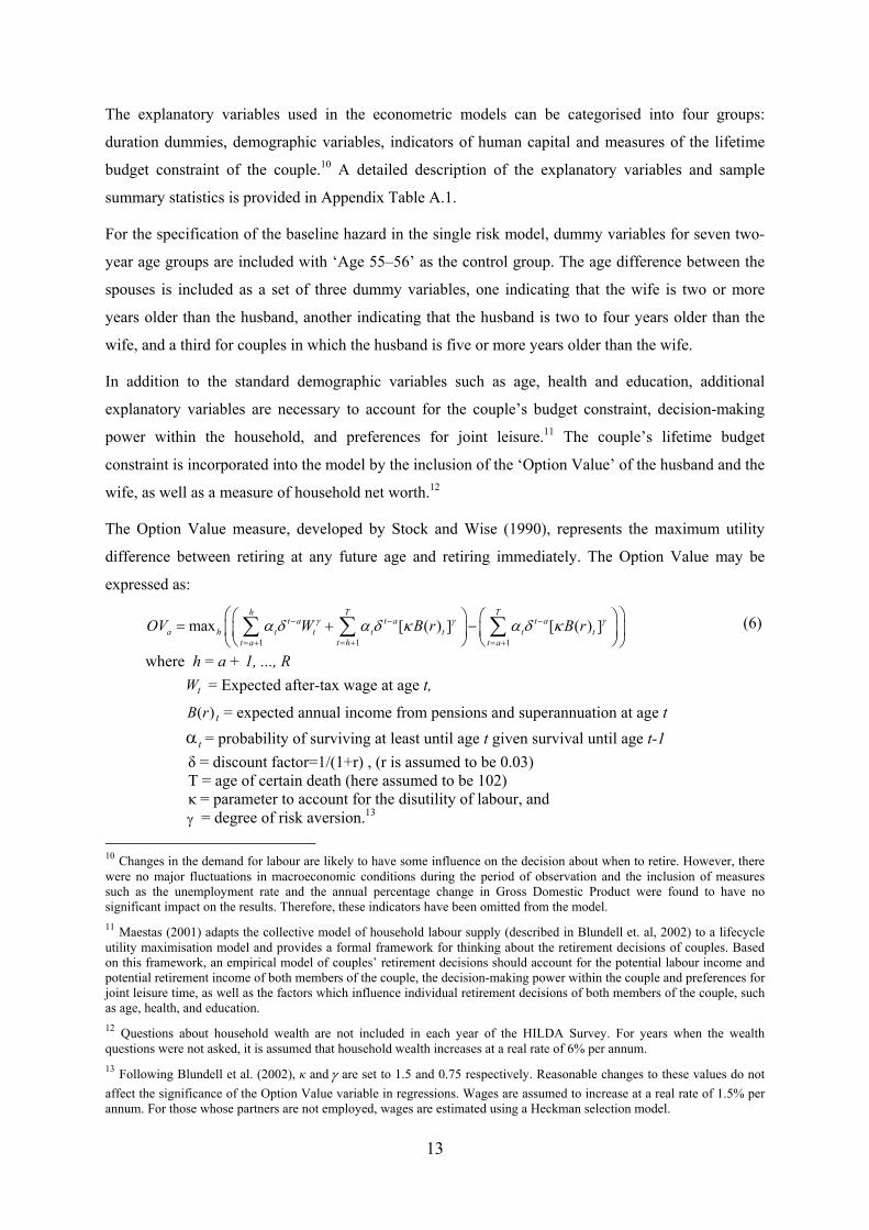
The Option Value measure, developed by Stock and Wise (1990), represents the maximum utility

difference between retiring at any future age and retiring immediately. The Option Value may be

expressed as:

1 1 1

max [ ( ) ] [ ( ) ]h T T

t a t a t aa h t t t t t t

t a t h t a

OV W B r B r

(6)

where h = a + 1, ..., R

tW = Expected after-tax wage at age t,

trB )( = expected annual income from pensions and superannuation at age t

t = probability of surviving at least until age t given survival until age t-1

δ = discount factor=1/(1+r) , (r is assumed to be 0.03) T = age of certain death (here assumed to be 102) κ = parameter to account for the disutility of labour, and = degree of risk aversion.13

10 Changes in the demand for labour are likely to have some influence on the decision about when to retire. However, there were no major fluctuations in macroeconomic conditions during the period of observation and the inclusion of measures such as the unemployment rate and the annual percentage change in Gross Domestic Product were found to have no significant impact on the results. Therefore, these indicators have been omitted from the model. 11 Maestas (2001) adapts the collective model of household labour supply (described in Blundell et. al, 2002) to a lifecycle utility maximisation model and provides a formal framework for thinking about the retirement decisions of couples. Based on this framework, an empirical model of couples’ retirement decisions should account for the potential labour income and potential retirement income of both members of the couple, the decision-making power within the couple and preferences for joint leisure time, as well as the factors which influence individual retirement decisions of both members of the couple, such as age, health, and education. 12 Questions about household wealth are not included in each year of the HILDA Survey. For years when the wealth questions were not asked, it is assumed that household wealth increases at a real rate of 6% per annum. 13 Following Blundell et al. (2002), κ and are set to 1.5 and 0.75 respectively. Reasonable changes to these values do not

affect the significance of the Option Value variable in regressions. Wages are assumed to increase at a real rate of 1.5% per annum. For those whose partners are not employed, wages are estimated using a Heckman selection model.

14

The Option Value measure is preferred over other financial incentive measures, such as the Accrual

and Peak values described by Gruber and Wise (2004), because it is the only measure that

incorporates potential labour income, potential income from pensions and superannuation, as well as

time preferences and survival probabilities.14 Negative coefficients for the effects of the Option Value

for the individual are expected. That is, the higher the utility from continuing to work, the lower the

likelihood of retirement.15 However, the size and significance of the incentive measures of the spouse

are uncertain, depending upon whether the income effect in the financial incentive outweighs the

effect of the preference for joint leisure. For example, a weak complementarity of leisure effect and

the income effect may roughly cancel each other out, leading to no overall response to spouses’

incentives, while a strong complementarity of leisure effect may outweigh the income effect, so that a

large financial incentive for one member of a couple to keep working encourages both spouses to stay

in the labour force (Coile, 2004).

Decision-making power within the household is accounted for by the inclusion of a measure of the

level of the husband’s control over household savings and investment in the previous year.16 In order

to capture preferences for joint leisure time, measures of the relationship satisfaction of the husband

and wife in the previous year are included as explanatory variables. The duration of the relationship

(sum of years married and cohabiting) and the relationship satisfaction of the husband and wife in the

previous year are also included as explanatory variables. It is hypothesised that the longer a couple

has been married or living together, the more influence one spouse will have on the other’s labour

force behaviour, and the higher the level of relationship satisfaction, the more likely that the couple

will have a preference for leisure time spent together.

The demographic variables included in the model account for the health, cultural background,

household composition and age difference of the couple. Indicators of the health status of both

members of the couple are included in the form of a dummy variable indicating whether the

individual has a health condition that limits their ability to work. There may also be cross-effects of

the health of one member of a couple on their spouse. The spouse might increase their labour supply

14 Expected income from pensions and superannuation is calculated according the income and assets tests for the Age Pension and the taxation rates for superannuation income that were in place in 2002, as these rules would be most likely to apply for the majority of the reference period. For further information about the calculation of potential retirement income, refer to Warren and Oguzoglu (2011). 15 In this sample, average Option Value is higher for women than for men. This is due to the fact that the average age of the women in this sample is lower than that of men; and as average levels of superannuation are lower for women than for men, women forego less in terms of potential retirement income by continuing on paid work until they reach age pension eligibility age.

16 Each year, respondents are asked to specify who makes the decisions about saving, investment and borrowing within their household. The responses of the husband and wife are averaged on a scale of 0 to 100, so that couples who agree that the wife is the main decision-maker have a score of zero, those who agree that these decisions are made together have a score of 50 and those who agree that the husband is the main decision-maker have a score of 100. If the husband says that he is the main decision-maker and the wife says that they decide together, their score will be 75. If the wife says that she is the main decision-maker and the husband says that decisions are shared, the couple’s score is 25.

15

to make up for the lost income resulting from their partner leaving employment, or reduce their labour

supply in order to care for their spouse.

Indicators of the human capital of both members of the couple are included in the form of a set of

education dummies, a measure of labour market experience (percentage of time since leaving full-

time education spent in paid employment) and occupational status. These variables capture both

earning capacity and employment opportunities.17

Indicators of the cultural background (born in a mainly English speaking or non-English speaking

country) of both the husband and the wife are included to account for any cultural differences that

may affect the timing of retirement relative to one’s spouse. A dummy variable indicating the

presence of resident children is also included. It is presumed that those with children still living at

home will be less likely to leave the labour force. Those who own their home outright are likely to

need less income than those who are renting or paying off a mortgage. Therefore, an indicator of

outright home ownership is included. A dummy variable for living in a major city is included to

account for the broad differences in labour market conditions and costs of living between

metropolitan and non-metropolitan areas. Individuals with high levels of job satisfaction are presumed

to be more likely to remain employed. Job satisfaction in the previous year is included for the

individual in the single risk model and for both members of the couple in the competing risks model.

To capture the effects of preferences for joint retirement, an indicator of whether the individual’s

spouse is employed is included in the single risk model.

4. Results

Before proceeding to the estimation of couples’ retirement decisions, we present some descriptive

evidence about the coordination of retirement among mature age couples who have already retired,

and the retirement intentions of those who have not yet retired. Average transition rates, computed by

comparing the distribution of couples in each (joint) labour force state in each year, conditional on

their labour force state in the previous year, are presented in Table 1.

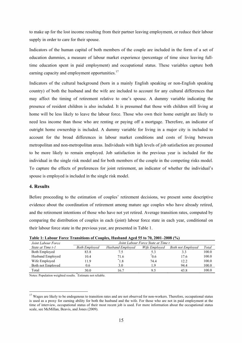
Table 1: Labour Force Transitions of Couples, Husband Aged 55 to 70, 2001–2008 (%) Joint Labour Force State at Time t-1

Joint Labour Force State at Time t Both Employed Husband Employed Wife Employed Both not Employed Total

Both Employed 83.8 7.5 5.3 3.3 100.0 Husband Employed 10.4 71.6 *0.6 17.6 100.0 Wife Employed 11.9 *1.8 74.4 12.2 100.0 Both not Employed 0.6 3.0 1.9 94.4 100.0Total 30.0 16.7 9.5 43.8 100.0

Notes: Population weighted results. *Estimate not reliable.

17 Wages are likely to be endogenous to transition rates and are not observed for non-workers. Therefore, occupational status is used as a proxy for earning ability for both the husband and the wife. For those who are not in paid employment at the time of interview, occupational status of their most recent job is used. For more information about the occupational status scale, see McMillan, Beavis, and Jones (2009).

16

During the eight year period from 2001 to 2008, the majority of mature age couples (74%) were either

in joint retirement (i.e. both not employed) or joint employment (husband and wife both employed).

There was a relatively high degree of persistence in the joint labour force status of couples from one

year to the next, with 94% of couples who were both not in paid employment and 84% couples who

were both employed still in the same situation one year later. There is also some evidence of joint

retirement. Of the 16% of couples who had made a transition out of the “both employed” category,

20% had moved to a situation in which neither member of the couple was employed. Furthermore,

compared to couples who were both employed in the previous period, there is a greater likelihood of

both members of a couple being out of the labour force if one member of the couple was not

employed in the previous year.

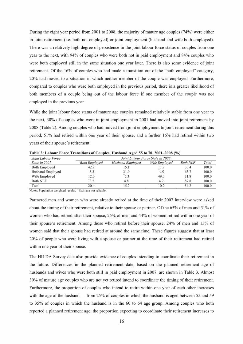
While the joint labour force status of mature age couples remained relatively stable from one year to

the next, 30% of couples who were in joint employment in 2001 had moved into joint retirement by

2008 (Table 2). Among couples who had moved from joint employment to joint retirement during this

period, 51% had retired within one year of their spouse, and a further 16% had retired within two

years of their spouse’s retirement.

Table 2: Labour Force Transitions of Couples, Husband Aged 55 to 70, 2001–2008 (%) Joint Labour Force State in 2001

Joint Labour Force State in 2008 Both Employed Husband Employed Wife Employed Both NLF Total

Both Employed 42.9 15.1 11.7 30.4 100.0 Husband Employed *5.3 31.0 *0.0 63.7 100.0 Wife Employed 12.0 *7.3 49.0 31.8 100.0 Both NLF *3.2 4.8 4.2 87.8 100.0 Total 20.4 15.2 10.2 54.2 100.0

Notes: Population weighted results. * Estimate not reliable.

Partnered men and women who were already retired at the time of their 2007 interview were asked

about the timing of their retirement, relative to their spouse or partner. Of the 65% of men and 31% of

women who had retired after their spouse, 25% of men and 44% of women retired within one year of

their spouse’s retirement. Among those who retired before their spouse, 24% of men and 13% of

women said that their spouse had retired at around the same time. These figures suggest that at least

20% of people who were living with a spouse or partner at the time of their retirement had retired

within one year of their spouse.

The HILDA Survey data also provide evidence of couples intending to coordinate their retirement in

the future. Differences in the planned retirement date, based on the planned retirement age of

husbands and wives who were both still in paid employment in 2007, are shown in Table 3. Almost

30% of mature age couples who are not yet retired intend to coordinate the timing of their retirement.

Furthermore, the proportion of couples who intend to retire within one year of each other increases

with the age of the husband — from 25% of couples in which the husband is aged between 55 and 59

to 35% of couples in which the husband is in the 60 to 64 age group. Among couples who both

reported a planned retirement age, the proportion expecting to coordinate their retirement increases to

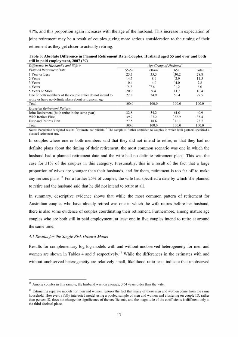
17

41%, and this proportion again increases with the age of the husband. This increase in expectation of

joint retirement may be a result of couples giving more serious consideration to the timing of their

retirement as they get closer to actually retiring.

Table 3: Absolute Difference in Planned Retirement Date, Couples, Husband aged 55 and over and both still in paid employment, 2007 (%) Difference in Husband’s and Wife’s Planned Retirement Date

Age Group of Husband 55-59 60-64 65+ Total

1 Year or Less 25.3 35.3 *30.2 28.8 2 Years 14.5 8.9 *2.9 11.5 3 Years 10.4 4.0 *4.0 7.8 4 Years *6.2 *7.6 *1.2 6.0 5 Years or More 20.9 9.4 11.2 16.4 One or both members of the couple either do not intend to retire or have no definite plans about retirement age

22.8 34.9 50.4 29.5

Total 100.0 100.0 100.0 100.0 Expected Retirement Pattern^ Joint Retirement (both retire in the same year) 32.8 54.2 61.0 40.9 Wife Retires First 39.7 27.2 *27.9 35.4 Husband Retires First 27.5 18.6 *11.1 23.7 Total 100.0 100.0 100.0 100.0 Notes: Population weighted results. *Estimate not reliable. ^ The sample is further restricted to couples in which both partners specified a planned retirement age.

In couples where one or both members said that they did not intend to retire, or that they had no

definite plans about the timing of their retirement, the most common scenario was one in which the

husband had a planned retirement date and the wife had no definite retirement plans. This was the

case for 31% of the couples in this category. Presumably, this is a result of the fact that a large

proportion of wives are younger than their husbands, and for them, retirement is too far off to make

any serious plans.18 For a further 25% of couples, the wife had specified a date by which she planned

to retire and the husband said that he did not intend to retire at all.

In summary, descriptive evidence shows that while the most common pattern of retirement for

Australian couples who have already retired was one in which the wife retires before her husband,

there is also some evidence of couples coordinating their retirement. Furthermore, among mature age

couples who are both still in paid employment, at least one in five couples intend to retire at around

the same time.

4.1 Results for the Single Risk Hazard Model

Results for complementary log-log models with and without unobserved heterogeneity for men and

women are shown in Tables 4 and 5 respectively.19 While the differences in the estimates with and

without unobserved heterogeneity are relatively small, likelihood ratio tests indicate that unobserved

18 Among couples in this sample, the husband was, on average, 3.64 years older than the wife.

19 Estimating separate models for men and women ignores the fact that many of these men and women come from the same household. However, a fully interacted model using a pooled sample of men and women and clustering on couple ID, rather than person ID, does not change the significance of the coefficients, and the magnitude of the coefficients is different only at the third decimal place.

18

heterogeneity is statistically significant for men and women. This may be an indicator of

complementarity in leisure that is not captured by the other variables included in the model.

Because of the non-linear nature of the complementary log-log model, the coefficients do not have a

straightforward interpretation. However, the antilog of the coefficients can be interpreted as the

hazard ratio. Hazard ratios are centred around 1, with a hazard ratio between 0 and 1 indicating a

decrease in the probability of retirement and a hazard ratio above 1 indicating an increase in the

probability of retirement. For example, the hazard ratio for men with a partner who is currently

employed is 0.135 in the model with gamma distributed frailty. This result indicates that for men who

have a partner who is currently employed, the hazard of retirement is 13.5% of the hazard rate for

those whose partner is not employed.

For men, health is found to be the most important determinant of retirement behaviour. Having a

work-limiting health condition more than triples the estimated hazard of retirement. The likelihood of

retirement also increases substantially for men in households where the family home is owned

outright; and is higher among men who completed year 12 compared to those who did not. As

expected, men with a higher Option Value have a lower retirement hazard. A 1,000 unit increase in

Option Value reduces the hazard of retiring by approximately 2 percentage points.20 While the

coefficients of the duration variables are not statistically significant, the duration variables at ages 65-

66 and 67-68 become statistically significant when the Option Value measure is excluded from the

model, reflecting eligibility for the Age Pension at age 65 that was previously captured by the Option

Value measure.

Among mature age men who are living with a spouse or partner, the hazard of retirement decreases

with the amount of control that they have over household decisions about saving and investment. It

may be the case that men who have more control over decisions about savings and investment also

have more control over decisions about when to retire. Alternatively, this may be a reflection of their

earning capacity. That is, those with higher earning capacity may also have more control over saving

and investment decisions within the household. The likelihood of retirement is also lower for men

who had higher levels of job satisfaction in the previous year, with a 1 point increase in job

satisfaction reducing the hazard of retirement by approximately 1 percentage point.

20 Estimates using alternative financial incentive measures are provided in Appendix Table A.2. Estimates using the Peak value (the maximum expected gain in lifetime retirement income from continuing in employment) are very similar to those using the Option Value. Estimates using the one-year Accrual measure (the maximum expected gain in lifetime retirement income from continuing in employment for one year) are slightly larger in magnitude, with a $1,000 increase in Accrual reducing the likelihood of retirement by approximately 6 percentage points. This is to be expected given the one-year Accrual measure represents an immediate change to which individuals should be more responsive.

19

Table 4: Probability of Retirement, Partnered Men Aged 55 to 70 and Employed in the Previous Year, Complementary log-log Estimates (Exponentiated Coefficients) No control for

unobserved heterogeneity Normally

distributed frailty Gamma

distributed frailty Hazard

Ratio Standard

Error Hazard Ratio

Standard Error

Hazard Ratio

Standard Error

Husband Age (Control = 55-56)

Age 57-58 0.501 [0.373] 0.563 [0.434] 0.596 [0.465] Age 59-60 0.738 [0.475] 0.867 [0.630] 0.703 [0.523] Age 61-62 1.288 [0.815] 1.619 [1.176] 1.400 [1.033] Age 63-64 1.181 [0.744] 1.473 [1.098] 1.353 [1.037] Age 65-66 1.256 [0.810] 1.619 [1.269] 1.717 [1.397] Age 67-68 1.442 [0.985] 1.942 [1.574] 2.299 [1.959] Age 69 and over 0.502 [0.363] 0.665 [0.575] 0.800 [0.722]

Work-limiting Health Condition 3.509*** [0.651] 3.955*** [0.819] 4.070*** [0.881] Country of Birth (Control = Australian Born)

MESB 0.882 [0.224] 0.919 [0.273] 0.994 [0.316] NESB 1.485 [0.453] 1.577 [0.524] 1.761 [0.609]

Education (Control = Year 11 or Below) Degree 0.769 [0.231] 0.692 [0.247] 0.560 [0.215] Certificate 0.943 [0.193] 0.971 [0.219] 0.968 [0.230] Year 12 1.855** [0.555] 1.911* [0.734] 2.084* [0.831]

Occupational Status 0.997 [0.004] 0.997 [0.005] 0.996 [0.005] Experience 0.991 [0.010] 0.985 [0.012] 0.983 [0.015] Option Value 0.979*** [0.004] 0.977*** [0.004] 0.980*** [0.005] Relationship Satisfaction (t -1) 1.011* [0.006] 1.010* [0.008] 1.010 [0.008] Job Satisfaction (t -1) 0.991 [0.006] 0.990* [0.006] 0.989* [0.006] Wife Age Difference (Control = Less than 2 Years Age Difference) Wife 2 or More Years Older 0.822 [0.304] 0.808 [0.336] 0.867 [0.379] Husband 2 to 4 Years Older 1.204 [0.239] 1.227 [0.292] 1.275 [0.322] Husband 5 or More Years Older 0.733 [0.209] 0.720 [0.232] 0.813 [0.276] Employed 0.193*** [0.041] 0.161*** [0.039] 0.135*** [0.035] Work-limiting Health Condition 0.955 [0.197] 1.060 [0.234] 1.092 [0.261] Country of Birth (Control = Australian Born)

MESB 1.903** [0.476] 1.912** [0.592] 1.598 [0.539] NESB 0.849 [0.310] 0.803 [0.313] 0.788 [0.321]

Education (Control = Year 11 or Below) Degree 0.817 [0.289] 0.941 [0.329] 1.033 [0.382] Certificate 1.184 [0.229] 1.214 [0.287] 1.304 [0.324] Year 12 0.340*** [0.135] 0.289*** [0.125] 0.253*** [0.118]

Occupational Status 1.006 [0.005] 1.005 [0.006] 1.007 [0.006] Experience 1.006* [0.003] 1.007* [0.004] 1.007* [0.004] Option Value 1.005*** [0.001] 1.005*** [0.002] 1.004** [0.002] Relationship Satisfaction (t -1) 0.994 [0.005] 0.993 [0.005] 0.993 [0.006] Household Own Home Outright 1.889*** [0.418] 2.168*** [0.601] 1.923** [0.557] Resident Children 0.710 [0.169] 0.698 [0.175] 0.629* [0.169] Relationship Duration 0.986 [0.010] 0.986 [0.012] 0.991 [0.013] Household Net Worth 0.926 [0.060] 0.925 [0.056] 0.941 [0.057] Major City 0.829 [0.156] 0.783 [0.162] 0.759 [0.167] Household Decision-maker (t -1) 0.476* [0.187] 0.396** [0.164] 0.405** [0.181] Log-likelihood -448.639 -447.219 -417.581 lnsig2u -0.687 (0.720) sigma_u 0.709 (0.255) rho/ gamma variance 0.234 (0.129) 0.500 (0.345) Likelihood-ratio test of rho/gamma var = 0 2.84** 62.12*** Note: ***, ** and * represent statistical significance at the 1%, 5% and 10% levels respectively.

20

For partnered men, the probability of retirement increases with their level of relationship satisfaction

in the previous year. This may be an indicator of a preference for joint retirement among couples with

high levels of relationship satisfaction. However, when gamma distributed frailty is included in the

model, this result is no longer statistically significant.21

The results concerning partner’s characteristics show some evidence of complementarity in leisure.

Compared to those whose partner is not in paid employment, men with a partner who is employed

have a substantially lower hazard of retirement.22 Men whose partner’s highest level of education is

Year 12 have a lower hazard of retirement than those whose partner did not complete Year 12. On the

other hand, partner’s Option Value has a small but statistically significant positive effect on the

hazard of retirement. It may be the case that some men whose wife has a strong financial incentive to

continue working may not be willing to delay their own retirement until their wife is ready to retire. 23

However, given that the retirement decisions of partnered women are more likely to influenced by

non-monetary factors such as caring responsibilities than financial considerations (Gruber and Wise,

2004), it stands to reason that men are not likely to base their decisions about retirement on the

financial incentives faced by their wives.

Turning now to the results for women, Table 5 shows that while health is a very important

determinant of men’s retirement behaviour, having a work-limiting health condition does not appear

to have a significant impact on the retirement decisions of partnered women. For women,

occupational status, labour market experience, job satisfaction and having children still living at home

all reduce the hazard of retiring.24

21 It is likely that those with high levels of relationship satisfaction are more likely to have a preference for leisure time with their partner. When partner’s labour force status is interacted with relationship satisfaction in the previous year, the results from the model with Gamma distributed frailty show that compared to men who had high levels of relationship satisfaction (80 or higher out of 100) in the previous year and whose partner was employed, the hazard of retirement was 9.24 times higher among men with high levels of relationship satisfaction and a partner who was not employed, but only 5.98 times higher among men with low levels of relationship satisfaction and a partner who was not employed. 22 It may be problematic to treat partner’s employment status as exogenous, as income from the Age Pension and other types of income support depend on partner’s income. Therefore, the financial incentive measures depend to some extent on whether an individual is part of a couple, and whether their partner is employed. When the model is estimated without the indicator of partner’s employment status, the Option Value remains highly significant, but the measure of control over household decisions is no longer statistically significant. 23 In calculating the Option Value for partners who were not in paid employment during the observation period, the potential labour market income component of the Option Value measure was estimated using a Heckman selection model. This may result in an over-estimate of the Option Value for partners who are not employed. However, the estimation results change very little when partner’s Option Value is excluded from the model, and when alternative measures of financial incentives that do not consider potential labour income are substituted for the Option Value measure (Table A.2). 24 For men, their own occupational status and the occupational status of their partner appear to have no significant impact on the retirement decision. However, for women, the probability of retirement is reduced as occupational status increases. When the occupational status measure is substituted for 1-digit indicators of occupation based on the ANZSCO 2006 occupation scale, we find that for men whose occupation is a labourer, the hazard of retirement is almost doubled. For women, the probability of retirement is reduced among those who are in professional occupations, and increased among women who are machinery operators or drivers, presumably due to the more physically demanding nature of these occupations. The likelihood of retirement is also higher for women whose spouse or partner’s current or most recent occupation was as a machinery operator or driver.

21

Table 5: Probability of Retirement, Partnered Women Aged 55 to 70 and Employed in the Previous Year, Complementary log-log estimates (Exponentiated Coefficients) No control for

unobserved heterogeneity Normally

distributed frailty Gamma

distributed frailty Hazard

Ratio Standard

Error Hazard Ratio

Standard Error

Hazard Ratio

Standard Error

Wife Age (Control = 55-56) Age 57-58 1.676 [1.177] 1.725 [1.465] 1.208 [1.012] Age 59-60 2.076 [1.402] 2.473 [2.110] 2.034 [1.685] Age 61-62 2.364 [1.662] 2.844 [2.543] 2.195 [1.919] Age 63-64 3.257 [2.428] 4.984 [4.982] 4.759 [4.670] Age 65-66 3.714* [2.934] 6.618* [7.048] 6.774* [7.123] Age 67-68 1.358 [1.335] 2.342 [2.865] 2.466 [3.037] Age 69 and over 1.969 [1.908] 2.800 [3.851] 2.543 [3.456] Work-limiting Health Condition 0.951 [0.315] 0.865 [0.329] 0.959 [0.370] Country of Birth (Control = Australian Born)

MESB 1.869 [0.802] 2.054 [1.037] 2.089 [1.085] NESB 1.070 [0.586] 0.982 [0.682] 1.277 [0.874]

Education (Control = Year 11 or Below) Degree 1.170 [0.572] 1.163 [0.665] 1.228 [0.706] Certificate 0.804 [0.260] 0.747 [0.272] 0.878 [0.316] Year 12 3.964** [2.131] 4.295* [3.231] 3.926* [2.943]

Occupational Status 0.981*** [0.006] 0.978** [0.009] 0.979** [0.008] Experience 0.988** [0.006] 0.987** [0.007] 0.989 [0.007] Option Value 1.005 [0.004] 1.007 [0.005] 1.007 [0.005] Relationship Satisfaction (t -1) 1.022* [0.013] 1.023** [0.012] 1.020* [0.012] Job Satisfaction (t -1) 0.983*** [0.007] 0.976*** [0.008] 0.976*** [0.008] Husband Age Difference (Control = Less than 2 Years Age Difference) Wife 2 or More Years Older 0.740 [0.383] 0.747 [0.423] 1.029 [0.569] Husband 2 to 4 Years Older 0.878 [0.310] 0.896 [0.339] 0.910 [0.351] Husband 5 or More Years Older 0.429* [0.205] 0.350* [0.189] 0.485 [0.259] Employed 0.264*** [0.093] 0.198*** [0.073] 0.193*** [0.071] Work-limiting Health Condition 0.770 [0.245] 0.681 [0.237] 0.579 [0.211] Country of Birth (Control = Australian Born)

MESB 1.668 [0.682] 1.728 [0.851] 1.546 [0.757] NESB 0.814 [0.357] 0.729 [0.397] 0.600 [0.338]

Education (Control = Year 11 or Below) Degree 0.991 [0.519] 1.212 [0.730] 1.234 [0.767] Certificate 0.803 [0.254] 0.887 [0.337] 0.898 [0.345] Year 12 0.362 [0.224] 0.340 [0.232] 0.399 [0.275]

Occupational Status 1.000 [0.007] 0.996 [0.008] 0.994 [0.008] Experience 1.030 [0.033] 1.023 [0.019] 1.023 [0.020] Option Value 0.993 [0.005] 0.991 [0.006] 0.990* [0.006] Relationship Satisfaction (t -1) 0.984 [0.010] 0.981* [0.011] 0.986 [0.011] Household Own Home Outright 1.331 [0.447] 1.543 [0.620] 1.489 [0.596] Resident Children 0.446** [0.171] 0.279** [0.151] 0.267** [0.147] Relationship Duration 0.995 [0.018] 0.998 [0.019] 1.006 [0.020] Household Net Worth 0.769* [0.108] 0.729* [0.118] 0.695** [0.117] Major City 1.070 [0.276] 1.172 [0.366] 1.280 [0.409] Household Decision-maker (t -1) 0.252** [0.166] 0.197** [0.146] 0.212** [0.159] Log-likelihood -228.109 -225.626 -214.040 lnsig2u 0.067 (0.637) sigma_u 1.034 (0.330) rho/ gamma variance 0.394 (0.152) 0.780 (0.458) Likelihood-ratio test of rho/gamma var = 0 6.27*** 29.45***

Note: ***, ** and * represent statistical significance at the 1%, 5% and 10% levels respectively.

22

For women, their own Option Value has no significant impact on the hazard of retirement. This result

confirms previous findings that for men, but not for women, the desire to maximise remaining lifetime

income, or the utility derived from it, is an important consideration in making the decision about when

to retire (Gruber and Wise, 2004; Warren and Oguzoglu, 2011). In seeking to understand this gender

difference, it is reasonable to point out that on average, superannuation savings of women are lower

than those of men; and in most households, men are still the main earners. Therefore, it is the

husband’s continuation or exit from the labour force that is going to have the most impact on the

household’s lifetime income. There is also a great deal of international evidence that compared with

men, women are more influenced by non-monetary factors including continuing caring

responsibilities and a preference for spending time with their spouse and other family members

(Gruber and Wise, 2004).

While their own Option Value has no significant impact on the retirement hazard for women, their

husband’s Option Value reduces the likelihood of retirement by approximately 1 percentage point per

1,000 units. Although this result is only significant at the 10% level, it suggests that some women may

delay their own retirement if their husband has a financial incentive to continue in paid work.25

Compared to women who did not complete high school, the retirement hazard for women whose

highest level of education is Year 12 is substantially higher. As was the case for men, having a partner

who is employed reduces the retirement hazard substantially, and those with higher levels of

relationship satisfaction have slightly higher hazards of retirement. The latter result suggests that there

is some evidence of complementarity in leisure.26

For women, the level of the husband’s control over decisions about household savings and

investments has a significant negative effect on the probability of retirement. Again, this may be a

reflection of the husband’s earning capacity, as husbands with a higher earning capacity may also

have more control over decisions about saving and investment.

In summary, the single risk hazard models provide some evidence of a preference for coordinated

retirement among mature age couples. For partnered men, health is a very important determinant of

retirement behaviour; and financial considerations, such as potential retirement income and home

ownership, are also significant factors in the decision about when to retire. On the other hand,

partnered women do not appear to base their retirement decisions on their own health or potential

25 When alternative measures of financial incentives are used, partner’s financial incentives are not statistically significant for women (Table A.2). This suggests that the husband’s potential labour income, which is only captured by the Option Value measure, is a more important consideration than the potential increase in his expected lifetime retirement income from delaying retirement. 26 For women, the difference in the hazard of retirement resulting from the interaction of partner’s employment status and their own relationship satisfaction is not as large as that for men. Compared to women who had high levels of relationship satisfaction in the previous year and whose partner was employed, the hazard of retirement was 4.26 times higher among women with high levels of relationship satisfaction and a partner who was not employed, and 3.62 times higher among men with low levels of relationship satisfaction and a partner who was not employed.

23

retirement income. However, it appears that some women may delay their own retirement if their

husband has a financial incentive to continue working, possibly due to complementarities in leisure.

Furthermore, having a partner who is employed reduces the retirement hazard substantially for both

men and women, which also suggests a preference among couples to retire together rather than

retiring alone.

4.2 Results for the Competing Risks Model

Results for the competing risks model, with and without unobserved heterogeneity are shown in

Tables 6 and 7 respectively. For ease of interpretation, the relative risk ratios (the anti-logged values

of the coefficients) are reported. The relative risk ratio measures the impact of a change in that

variable on the probability of exiting employment to that destination, relative to the probability of

remaining in employment. For example, in the model without unobserved heterogeneity, the relative

risk ratio for the husband’s Option Value is 0.978 for the destination state of ‘husband retires first’

(Table 6). According to this result, the probability of the husband retiring first, relative to the

probability of both members of the couple remaining in employment, is reduced by 2.2 percentage

points for every 1,000 units of the husband’s Option Value.

When unobserved heterogeneity is included in the model in the form of a random effect, the results

are, in general, not substantially different from those of the model without unobserved heterogeneity.

The main difference between the two sets of results is that the magnitude of the coefficients is reduced

slightly when unobserved heterogeneity is included. For the outcome of the wife retiring before the

husband, the education level of both the husband and the wife become insignificant in the model with

unobserved heterogeneity. Relationship duration also becomes statistically insignificant once

unobserved heterogeneity is controlled for. The remainder of the discussion of the results of the

competing risk model refers to the estimates in which unobserved heterogeneity is included in the

model (Table 7).

From Table 7, it is immediately evident that some regression coefficients vary by destination state.

The likelihood of a husband retiring before his wife is mainly due to health considerations, and to a

lesser extent to financial considerations. More specifically, the probability of the husband retiring

before his wife is ten times higher among couples in which the husband has a work-limiting health

condition. Owning a home outright triples the odds of a husband retiring before his wife; while the

odds of a husband retiring before his wife decrease slightly with the husband’s Option Value, labour

market experience and household net worth. However, none of the wife’s attributes are significant for

this outcome.

24

Table 6: Competing Risks Estimates, without Unobserved Heterogeneity (Relative Risk Ratios) Husband

retires first Wife

retires first Joint

retirement

RRR S.E. RRR S.E. RRR S.E.Husband Age (Control = 55-60) Age61-62 2.770** [1.332] 0.752 [0.315] 2.260 [1.468] Age63-64 1.638 [0.916] 0.765 [0.348] 4.066** [2.618] Age65-66 1.961 [1.379] 0.628 [0.385] 5.991** [4.944] Age67-70 1.938 [1.473] 1.080 [0.630] 6.359** [5.573] Work-limiting Health Condition 7.498*** [2.834] 0.941 [0.367] 4.124*** [1.823] Country of Birth (Control = Australian Born)

MESB 0.702 [0.388] 0.971 [0.450] 0.666 [0.477] NESB 1.011 [0.544] 0.452 [0.252] 1.021 [0.709]

Highest Level of Education (Control = Year 11 or Below) Degree 1.182 [0.728] 0.351* [0.198] 2.489 [2.002] Certificate 0.880 [0.401] 0.549* [0.190] 1.130 [0.523] Year 12 1.585 [1.046] 0.302* [0.196] 1.970 [1.409]

Occupational Status 0.995 [0.009] 1.012 [0.008] 0.986 [0.010] Experience 0.956 [0.027] 0.987 [0.025] 0.982 [0.037] Option Value 0.978*** [0.008] 0.985** [0.006] 0.982* [0.010] Job Satisfaction (t -1) 0.998 [0.010] 1.034*** [0.011] 0.987 [0.011] Relationship Satisfaction (t -1) 1.003 [0.014] 0.966*** [0.010] 1.014 [0.019] Wife Age Difference Between Husband and Wife (Control = Less than 2 Years Age Difference)

Wife 2 or More Years Older 0.284 [0.377] 0.896 [0.856] 4.531 [4.366] Husband 2 to 4 Years Older 1.349 [0.747] 1.065 [0.379] 1.078 [0.541] Husband 5 or More Years Older 1.219 [0.780] 0.298** [0.156] 0.237* [0.185]

Work-limiting Health Condition 1.106 [0.581] 0.822 [0.369] 0.836 [0.447] Country of Birth (Control = Australian Born)

MESB 2.042 [1.177] 3.766*** [1.876] 2.385 [1.804] NESB 1.769 [1.154] 1.168 [0.739] 0.535 [0.543]

Highest Level of Education (Control = Year 11 or Below) Degree 2.301 [1.335] 1.753 [0.853] 0.361 [0.322] Certificate 1.671 [0.770] 0.595 [0.237] 0.406* [0.221] Year 12 0.416 [0.316] 2.662* [1.399] 0.137* [0.163]

Occupational Status 1.008 [0.010] 0.981** [0.009] 0.979 [0.013] Experience 1.006 [0.009] 0.986** [0.006] 0.994 [0.008] Option Value 1.001 [0.003] 0.998 [0.003] 1.006 [0.005] Job Satisfaction (t -1) 1.006 [0.010] 0.967*** [0.007] 0.972*** [0.010] Relationship Satisfaction (t -1) 0.992 [0.010] 1.020* [0.011] 1.001 [0.013] Household Resident Children 1.381 [0.617] 0.287** [0.139] 1.304 [0.717] Relationship Duration 0.963* [0.019] 0.971* [0.017] 1.029 [0.036] Household Net Worth 0.579** [0.129] 0.802** [0.089] 0.873 [0.111] Own Home Outright 2.595* [1.380] 1.065 [0.380] 0.647 [0.306] Major City 0.893 [0.361] 2.256** [0.713] 3.424*** [1.567] Household Decision-maker (t -1) 0.695 [0.542] 5.371** [3.669] 0.252 [0.261] Log likelihood = -464.263 N = 916 Pseudo R2 = 0.2342 Note: ***, ** and * represent statistical significance at the 1%, 5% and 10% levels respectively.

25

Table 7: Competing Risks Estimates, with Unobserved Heterogeneity (Relative Risk Ratios) Husband

retires first Wife

retires first Joint

retirement

RRR S.E. RRR S.E. RRR S.E.Husband Age (Control = 55-60) Age61-62 3.274** [1.706] 0.847 [0.384] 2.643 [1.822] Age63-64 2.051 [1.261] 0.864 [0.438] 5.075** [3.548] Age65-66 2.462 [1.911] 0.848 [0.587] 8.415** [7.605] Age67-70 2.525 [2.129] 1.464 [0.999] 9.244** [8.889] Work-limiting Health Condition 10.416**

*[4.625] 1.169 [0.523] 5.199*** [2.553]

Country of Birth (Control = Australian Born) MESB 0.732 [0.449] 0.844 [0.456] 0.684 [0.523] NESB 1.022 [0.630] 0.388 [0.252] 0.933 [0.718] Highest Level of Education (Control = Year 11 or Below) Degree 1.060 [0.767] 0.383 [0.257] 2.623 [2.355] Certificate 0.799 [0.417] 0.613 [0.257] 1.212 [0.635] Year 12 1.522 [1.141] 0.351 [0.261] 2.201 [1.784] Experience 0.940* [0.031] 0.975 [0.030] 0.966 [0.040] Occupational Status 0.994 [0.010] 1.015* [0.009] 0.989 [0.011] Option Value 0.975*** [0.009] 0.982** [0.007] 0.980* [0.010] Job Satisfaction (t -1) 0.998 [0.011] 1.036*** [0.013] 0.988 [0.012] Relationship Satisfaction (t -1) 0.999 [0.015] 0.962*** [0.011] 1.008 [0.020] Wife Age Difference Between Husband and Wife (Control = Less than 2 Years Age Difference) Wife 2 or More Years Older 0.195 [0.299] 0.871 [0.992] 3.583 [4.022] Husband 2 to 4 Years Older 1.356 [0.825] 1.076 [0.466] 0.982 [0.548] Husband 5 or More Years Older 0.881 [0.637] 0.228** [0.138] 0.162** [0.136] Work-limiting Health Condition 0.985 [0.559] 0.812 [0.405] 0.833 [0.482] Country of Birth (Control = Australian Born) MESB 2.648 [1.765] 4.885*** [2.871] 2.865 [2.354] NESB 1.814 [1.364] 1.314 [0.985] 0.610 [0.665] Highest Level of Education (Control = Year 11 or Below) Degree 2.633 [1.738] 1.511 [0.872] 0.336 [0.311] Certificate 1.741 [0.915] 0.617 [0.290] 0.479 [0.281] Year 12 0.404 [0.340] 2.354 [1.491] 0.098* [0.131] Experience 1.003 [0.010] 0.985** [0.007] 0.994 [0.009] Occupational Status 1.008 [0.012] 0.981* [0.010] 0.977* [0.014] Option Value 1.003 [0.004] 0.999 [0.003] 1.008 [0.005] Job Satisfaction (t -1) 1.002 [0.011] 0.963*** [0.009] 0.969*** [0.010] Relationship Satisfaction (t -1) 0.992 [0.011] 1.025** [0.013] 1.005 [0.015] Household Resident Children 1.290 [0.646] 0.236*** [0.129] 1.141 [0.688] Relationship Duration 0.963* [0.022] 0.971 [0.019] 1.034 [0.038] Household Net Worth 0.945** [0.022] 0.977* [0.012] 0.985 [0.013] Own Home Outright 2.992* [1.759] 1.009 [0.418] 0.708 [0.371] Major City 0.915 [0.409] 2.265** [0.843] 3.435** [1.728] Household Decision-maker (t -1) 0.644 [0.563] 7.818** [6.328] 0.245 [0.273] Log likelihood = -461.458 N = 916 Variance of random effect = 0.937 (0.585) Note: ***, ** and * represent statistical significance at the 1%, 5% and 10% levels respectively.

Turning to the scenario in which the wife retires before her husband, it is evident from Table 7 that

the characteristics and preferences of both members of the couple have a significant impact on the

likelihood of this outcome. For example, the likelihood of a wife retiring before her husband increases

with the husband’s job satisfaction and occupational status, and decreases with the husband’s Option

Value. The latter result suggests that some women may delay retirement if their husband has a

financial incentive to do so. The husband’s level of relationship satisfaction in the previous year also

26

has a significant effect on the likelihood of this outcome. This suggests that in couples where the

husband has a high level of relationship satisfaction, the wife may delay her own retirement in order

to retire at the same time as her husband. However, women with high levels of relationship

satisfaction in the previous year are more likely to retire before their husband. One possible

explanation for this result is that for women, high levels of relationship satisfaction do not necessarily

coincide with a stronger preference for joint retirement.

Women born in an English speaking country other than Australia are more likely to retire before their

husbands, as are women living in major cities and the odds of a wife retiring before her husband

increase with the decision-making power of the husband. Conversely, the likelihood of a wife retiring

before her husband decreases with the wife’s occupational status, labour market experience and job

satisfaction, and are decreased substantially the husband is at least 5 years older than his wife, and

also if the couple has children still living at home.

Compared to couples in which the husband is aged between 55 and 60, the odds of joint retirement are

increased considerably if the husband is aged 65 or older. In couples where the wife is younger than

the husband, this may be a result of both members of the couple reaching Age Pension eligibility

age.27 The odds of joint retirement are substantially higher if the husband has a work-limiting health

condition, which implies that women are likely to retire in order to care for their husband, but the

opposite is not the case. It also appears that for couples, the coordination of retirement differs between

rural and urban areas, as the likelihood of joint retirement is higher among couples living in major

cities. On the other hand, the probability of joint retirement decreases with the job satisfaction of the

wife, and is also reduced if the husband is at least five years older than his wife. These results suggest

that women with high levels of job satisfaction and women who are at least five years younger than

their husband are less likely to be willing to retire early in order to coordinate their retirement with

their spouse. The likelihood of joint retirement also decreases with the husband’s Option Value.

Although this result is only significant at the 10% level, it suggests that both members of a couple

may delay retirement if the husband has a financial incentive to do so.28

As the purpose of the competing risks model is to determine the factors associated with the timing of

retirement for couples, it is interesting to examine the effects of financial incentives at a couple level,

rather than at an individual level. For example, the one-year Accrual for the couple if the husband and

the wife both delay retirement for one year (i.e. the gain in total expected remaining lifetime

27 This result should be interpreted with caution due to the limited number of couples in these age categories. 28 Estimates of the competing risk model using alternative financial incentive measures are provided in Table A.3. As was the case for the single risk model, the individual Accrual and Peak values for the wife are not statistically significant; the results concerning the Peak value for the husband are very similar to those for the Option Value; and the magnitude of the effect of the one-year Accrual for the husband are larger than those of the Peak or Option Value measures. However, for the outcome of the husband retiring first, the Peak value is not statistically significant. This result suggests that for this outcome, potential labour income foregone if the husband retires (which is captured by the Option Value measure but not the Peak value) is a more important consideration than his potential retirement income from pensions and superannuation.

27

retirement income for the couple if the husband and wife both delay retirement for one year); or the

Peak value of the couple — the maximum possible gain in total expected remaining lifetime

retirement income for the couple if the husband and wife both delay retirement until a later date.

Estimates of the competing risk model using alternative financial incentive measures are provided in

Table A.3.

When the individual Option Values are replaced by the one-year Accrual for the couple, the

estimation results indicate that the likelihood of the wife retiring first, and also that of joint retirement,

decrease by 4 to 5 percentage points for every $1,000 of the Accrual value of the couple. In other

words, if there is an overall financial incentive for the couple to delay retirement for one year, the

likelihood of joint retirement and the wife retiring before her husband is reduced. Similarly, when the

individual Option Values are replaced by the Peak value for the couple, the likelihood of the wife

retiring first is reduced by 1.5 percentage points for every $1,000 of the couple’s Peak value. These

results support the conclusion that women may delay their retirement if their husband, or the couple

overall, has a financial incentive to continue working.29

In summary, competing risks models examining the timing of an individual’s retirement relative to

their spouse indicate that the situation in which a husband retires before his wife is likely to be a result

of his own poor health, and to a lesser extent to financial considerations. However, none of the wife’s

attributes are significant for this outcome. On the other hand, the odds of a wife retiring before her

husband are affected by the characteristics and preferences of both members of the couple; increasing

with the husband’s job satisfaction, occupational status and decision-making power within the

household; and decreasing with the occupational status, labour market experience and job satisfaction

of the wife; if the couple has resident children and if the husband is older than the wife by five years

or more. The likelihood of the wife retiring before her husband decreases with the husband’s Option

Value, which suggests that women may delay retirement if their husband has a financial incentive to

remain in employment. Using ‘couple level’ measures of financial incentives further supports the

conclusion that women may delay their retirement if their husband, or the couple overall, has a

financial incentive to continue working. The odds of joint retirement increase considerably if the

husband has a work-limiting health condition. This result suggests that women are likely to retire in

order to care for their husband, but the opposite is not the case, presumably due to the reduction in

household income resulting from the husband leaving paid employment to care for his wife.

29 These combined measures of the financial incentives faced by couples do not account for differences in the financial incentives faced by husbands and wives. For example, one member of a couple may have a strong financial incentive to delay retirement, but the other may not. Including the difference between the Accrual values of the husband and the wife in addition to the couple level Accrual does not change the result concerning couple’s Accrual (Table A.3). When the individual Peak values of the husband and the wife are included along with the Peak value of the couple together, the results indicate that the likelihood of the husband retiring first is reduced with the couple’s overall Peak value, but increases with the Peak value of the wife. This result is similar to that of the single risk models for men, which suggest that men are not likely to delay their own retirement in response to the financial incentives faced by their wife.

28

5. Conclusion

Descriptive evidence from the HILDA Survey shows that, while the most common pattern of

retirement for Australian couples is one in which the wife retires before the husband, there is some

evidence of couples coordinating their retirement. Furthermore, among mature age couples who are

not yet retired, at least one in five intend to retire at approximately the same time.

Single and competing risk duration models are estimated to investigate the determinants of the

retirement decisions of partnered men and women. Both models provide evidence of a preference for

coordinated retirement among mature age couples. For partnered men, their own health is a very

important determinant of retirement behaviour; and financial considerations, such as potential

retirement income and home ownership, are also significant factors in the decision about when to

retire. However, partnered women do not appear to base their retirement decisions on their own health

or potential retirement income, but may delay their own retirement if their partner has a financial

incentive to continue working. Furthermore, competing risk estimates show that the likelihood of joint

retirement is considerably higher if the husband has a work-limiting health condition. That is, women

are likely to retire to care for their husband, but the opposite is not the case.

The models estimated in this paper show that Australian couples' retirement choices are determined

by individual and job characteristics, and also to some extent by partner’s and couple’s characteristics.

These results suggest that complementarity in leisure is an important consideration in the retirement

decisions of partnered men and women. This finding has important implications for policymakers. It

implies that any policy affecting the retirement decision of one member of a couple, for example,

changes to the eligibility requirements for the Age Pension, will have flow-on effects to the retirement

behaviour of their partner. Therefore, modeling the retirement behaviour of partnered men and women

without considering the characteristics and preferences of their partner is likely to lead to errors in

predicting the impact of changes in Social Security policy on retirement behaviour.

29

APPENDIX

Table A.1: Variables Included in Multivariate Analyses Men Women Couples Mean S.E. Mean S.E. Mean S.E. Individual Information Age 57 or 58 0.116 0.008 0.186 0.015 0.123 0.011 Age 59 or 60 0.190 0.010 0.220 0.016 0.201 0.013 Age 61 or 62 0.225 0.011 0.247 0.017 0.230 0.014 Age 63 or 64 0.191 0.010 0.154 0.014 0.195 0.013 Age 65 or 66 0.121 0.009 0.082 0.011 0.109 0.010 Age 67 or 68 0.080 0.007 0.048 0.008 0.075 0.009 Age 69 and older 0.054 0.006 0.022 0.006 0.041 0.007 Work-limiting health condition 0.152 0.009 0.123 0.013 0.164 0.012 Born in a mainly English speaking country 0.147 0.009 0.100 0.011 0.144 0.012 Born in a non-English speaking country 0.130 0.009 0.094 0.011 0.126 0.011 Degree qualification 0.210 0.011 0.185 0.015 0.211 0.013 Trade certificate, diploma or other certificate level qualification 0.422 0.013 0.298 0.018 0.414 0.016 Highest qualification is Year 12 0.074 0.007 0.034 0.007 0.084 0.009 Occupation status in current job 50.250 0.645 50.439 0.859 50.387 0.814 Percentage of years in paid work since leaving full-time education 96.861 0.187 76.215 0.850 97.292 0.172 Option Value (’000) 46.262 1.067 61.630 1.961 48.942 1.370 Job satisfaction in the previous year (out of 100) 81.598 0.440 83.583 0.637 81.146 0.585 Relationship satisfaction in the previous year (out of 100) 89.314 0.376 87.004 0.586 88.657 0.492 Partner Information Wife older than husband by 2 or more years 0.062 0.006 0.181 0.015 0.024 0.005 Husband 2 to 4 years older than wife 0.336 0.012 0.311 0.018 0.318 0.015 Husband 5 or more years older than wife 0.357 0.013 0.157 0.014 0.434 0.016 Indicator of whether partner is employed 0.579 0.013 0.742 0.017 0.879 0.011 Work-limiting health condition 0.167 0.010 0.225 0.016 0.118 0.011 Born in a mainly English speaking country 0.102 0.008 0.142 0.013 0.088 0.009 Born in a non-English speaking country 0.091 0.008 0.119 0.012 0.070 0.008 Degree qualification 0.201 0.010 0.260 0.017 0.225 0.014 Trade certificate or other certificate level qualification 0.206 0.011 0.386 0.019 0.225 0.014 Highest qualification is Year 12 0.091 0.008 0.087 0.011 0.080 0.009 Occupational status in current or most recent job 47.286 0.574 50.533 0.944 76.228 0.764 Percentage of years in paid work since leaving full-time education 65.789 0.735 94.645 0.329 50.345 0.722 Option Value (’000) 70.944 1.362 48.582 1.586 73.248 1.795 Relationship satisfaction in the previous year (out of 100) 86.187 0.462 89.618 0.480 85.895 0.581 Job satisfaction in the previous year (out of 100) - - - - 81.277 0.607 Household Information Own home outright 0.771 0.011 0.777 0.016 0.749 0.014 Has resident children under the age of 15 0.227 0.011 0.142 0.013 0.235 0.014 Total time cohabiting with and/or married to current partner (years) 33.64 0.257 34.72 0.373 32.39 0.340 Household Net Worth (Total assets – Total Debt, $’000) 141.12 4.919 145.40 7.581 146.42 6.352 Live in a major city 0.571 0.013 0.521 0.019 0.515 0.017 Husband’s decision-making power in previous year (out of 100) 0.574 0.006 0.474 0.008 0.543 0.007 Alternative Financial Incentive Measures Accrual ($’000) -3.130 0.023 -2.238 0.213 -2.417 0.248 Partner’s Accrual ($’000) 0.471 0.190 -2.360 0.275 0.912 0.244 Peak Value ($’000) 1.057 0.533 2.082 0.808 2.696 0.731 Partner’s Peak Value ($’000) 15.422 0.908 1.941 0.665 17.711 1.304 Accrual For Couple ($’000) — — — — -1.504 0.378 Peak Value for Couple ($’000) — — — — 11.740 1.373 N 1458 681 916

30

Table A.2: Single Risk Estimates Using Alternative Financial Incentive Measures, Complementary log-log Estimates (Exponentiated Coefficients) No control for

unobserved heterogeneity Normally

distributed frailty Gamma

distributed frailty Coef. S.E. Coef. S.E. Coef. S.E. Men Option Value (‘000) 0.979*** [0.004] 0.977*** [0.004] 0.980*** [0.005] Partner’s Option Value (‘000) 1.005*** [0.001] 1.005*** [0.002] 1.004** [0.002]

Accural ($‘000) 0.944*** [0.012] 0.933*** [0.014] 0.932*** [0.015] Partner’s Accrual ($‘000) 1.020* [0.012] 1.027* [0.015] 1.028* [0.103]

Peak Value ($‘000) 0.972*** [0.011] 0.967*** [0.009] 0.971*** [0.010] Partners Peak Value ($‘000) 1.007*** [0.002] 1.007** [0.003] 1.006 [0.004] Women Option Value (‘000) 1.005 [0.004] 1.007 [0.005] 1.007 [0.005] Partner’s Option Value (‘000) 0.993 [0.005] 0.991 [0.006] 0.990* [0.006]

Accural ($‘000) 0.986 [0.024] 0.988 [0.032] 0.985 [0.031] Partner’s Accrual ($‘000) 0.986 [0.025] 0.972 [0.028] 0.970 [0.028]

Peak Value ($‘000) 0.997 [0.013] 1.001 [0.014] 1.003 [0.015] Partners Peak Value ($‘000) 0.987 [0.015] 0.983 [0.015] 0.976 [0.016]

Note: ***, ** and * represent statistical significance at the 1%, 5% and 10% levels respectively. Social Security Wealth (SSW) is the present value of expected total remaining lifetime income from the Age Pension and superannuation. SSW Accrual is the difference in SSW the individual continues working for one year, compared to SSW from immediate retirement. The Peak value is difference between the maximum possible value of SSW from continuing in employment until a later date, and SSW from immediate retirement. If there is no potential gain in SSW from delaying retirement until a later date, the Peak value is equal to the Accrual value.

Table A.3: Competing Risks Estimates using Alternative Financial Incentive Measures, with Unobserved Heterogeneity (Relative Risk Ratios) Wife

retires firstHusband

retires firstJoint

retirement RRR S.E. RRR S.E. RRR S.E.

Husband’s Option Value 0.982** [0.007] 0.975*** [0.009] 0.980* [0.010] Wife’s Option Value 0.999 [0.003] 1.003 [0.004] 1.008 [0.005]

Husband’s Accrual 0.929*** [0.023] 0.943** [0.028] 0.916** [0.034] Wife’s Accrual 0.999 [0.026] 1.006 [0.029] 0.992 [0.039]

Husband’s Peak Value 0.970** [0.015] 0.978 [0.016] 0.956* [0.024] Wife’s Peak Value 0.995 [0.007] 1.006 [0.006] 1.006 [0.011]

Accrual for Couple 0.962** [0.015] 0.974 [0.018] 0.952** [0.020]

Accrual for Couple 0.963** [0.016] 0.974 [0.018] 0.953** [0.020] Difference between Husband’s and Wife’s Accrual 0.964* [0.019] 0.968 [0.023] 0.961 [0.030] Peak Value for Couple 0.985** [0.007] 0.991 [0.007] 0.989 [0.010] Peak Value for Couple 1.001 [0.020] 0.973** [0.014] 1.010 [0.034] Husband’s Peak Value 0.968 [0.028] 1.010 [0.020] 0.944 [0.046] Wife’s Peak Value 0.995 [0.014] 1.021** [0.009] 1.000 [0.025]

Note: ***, ** and * represent statistical significance at the 1%, 5% and 10% levels respectively. Social Security Wealth (SSW) is the present value of expected total remaining lifetime income from the Age Pension and superannuation. SSW Accrual is the difference in SSW the individual continues working for one year, compared to SSW from immediate retirement. The Peak value is difference between the maximum possible value of SSW from continuing in employment until a later date, and SSW from immediate retirement. If there is no potential gain in SSW from delaying retirement until a later date, the Peak value is equal to the Accrual value. The Accrual value for a couple is the sum of the Accrual values of the husband and the wife. The Peak value for a couple is the difference between the maximum possible gain in combined SSW for the husband and the wife if they both delay retirement until a later date, compared to their combined SSW if they both retire immediately. Estimates not accounting for unobserved heterogeneity are very similar, the significance of the coefficients does not change and their magnitude differs only at the third decimal place.

31

References

An, M., Christensen, B. J. and Datta Gupta, N. (2004) ‘Multivariate Mixed Proportional Hazard Modelling of the Joint Retirement of Married Couples’, Journal of Applied Econometrics, vol. 19, pp. 687–704.

Baker, M. (1999) ‘The Retirement Behavior of Married Couples: Evidence from the Spouse’s Allowance’, Journal of Human Resources, vol. 37, no. 1, pp. 1–34.

Blau, D. (1998) ‘Labor Force Dynamics of Mature Age Couples’, Journal of Labor Economics, vol. 16, no. 3. pp. 595–629.

Blau, D. and Gilleskie, D. (2006) ‘Health Insurance and Retirement of Married Couples’, Journal of Applied Econometrics, vol. 21, no. 7, pp. 935–953.

Blau, D. and Riphahn, R. (1999) ‘Labor Force Transitions of Older Married Couples in Germany’, Labour Economics, vol. 6, no. 2, pp. 229–251.

Blundell, R., Meghir, C. and Smith, S. (2002) ‘Pension Incentives and the Pattern of Early Retirement’, Economic Journal, vol. 112, no. 478, pp. C153–170.

Browning, M. (2000) ‘The Savings Behaviour of a Two Person Household’, Scandinavian Journal of Economics, vol. 102, no. 2, pp. 235–251.

Cobb-Clark, D. and Stillman, S. (2009) ‘The Retirement Expectations of Middle-aged Individuals’, Economic Record, vol. 85, no. 269, pp. 146–163.

Coile, C. (2004) ‘Retirement Incentives and Couple’s Retirement Decisions’, Topics in Economic Analysis and Policy, vol. 4, no. 1, article 17.

Cox, D. (1972) ‘Regression Models and Life Tables’, Journal of the Royal Statistical Society, Series B (Methodological), vol. 34, no. 2, pp. 187–220.

de Vaus, D. and Wells, Y. (2003) ‘I Married Him for Better or for Worse but Not for Lunch: Retirement and Marriage’, Paper presented at the 8th Australian Family Research Conference, Melbourne, 12–14 February.

Deschryvere, M. (2005) ‘Labour Force Behaviour of Men and Women in Elderly Two-adult Households, Evidence from EU Countries’, ENEPRI Research Report No. 7, European Network of Research Policy Institutes.

Gruber, J. and Wise, D. (2004) Social Security Programs and Retirement around the World: Micro-estimation, University of Chicago Press, Chicago.

Gustman, A. and Steinmeier, T. (1994) ‘Retirement in a Family Context: A Structural Model for Husbands and Wives’, Working Paper No. 4629, National Bureau of Economic Research, Cambridge, MA.

Gustman, A. and Steinmeier, T. (2000) ‘Retirement in Dual-Career Families: A Structural Model’, Journal of Labor Economics, vol. 18, no. 3, pp. 503–545.

Gustman, A. and Steinmeier, T. (2002) ‘Social Security, Pensions and Retirement Behavior within the Family’, Working Paper No. 8772, National Bureau of Economic Research, Cambridge, MA.

Gustman, A. and Steinmeier, T. (2004) ‘Social Security, Pensions and Retirement Behaviour Within the Family’, Journal of Applied Econometrics, vol. 19, no. 6, pp. 723–737.

Hurd, M. (1990) ‘The Joint Retirement Decisions of Husbands and Wives’, In D. Wise (ed.) Issues in the Economics of Aging, pp. 231–254, University of Chicago Press, Chicago.

Jenkins, S. (2005) ‘Survival Analysis’, Unpublished Manuscipt, Institute for Social and Economic Research, University of Essex, Colchester, UK, <http://www.iser.essex.ac.uk/iser/ teaching/module-ec968>.

32

Jiménez-Martín, S., Labeaga, J. and Granado, M. (1999) ‘Health Status and Retirement Decisions for Older European Couples’, IRISS Working Paper No. 1999–01, Centre for Population, Poverty and Public Policy Studies, Luxembourg.

Johnson, R. and Favreault, M. (2001) ‘Retiring Together or Working Alone — The Impact of Spousal Employment and Disability on Retirement Decisions’, Working Paper No. 2001–01, Center for Retirement Research at Boston College.

Kapur, K. and Rogowski, J. (2006) ‘The Role of Health Insurance in Joint Retirement among Married Couples’, Working Paper No. 06/14, University College Dublin School of Economics.

Knox, G. (2003) ‘Retirement Intentions of Mature Age Workers’, Paper presented at the Australian Social Policy Conference, University of New South Wales, 9–11 July.

McMillan, J., Beavis, A. and Jones, F. (2009) ‘The AUSEI06: A New Socioeconomic Index for Australia’, Journal of Sociology, vol. 45, no. 2, pp. 123–149.

Maestas, N. (2001) ‘Labour, Love and Leisure: Complementarity and the Timing of Retirement by Working Couples’, mimeo, Department of Economics, University of California, Berkeley.

Michaud, P. (2003) ‘Joint Labour Supply Dynamics of Older Couples’, Discussion Paper No. 832, Institute for the Study of Labor (IZA), Bonn.

Pozzoli, D. and Ranzani, M. (2009) ‘Old European Couple’s Retirement Decisions: The Role of Love and Money’, Working Paper No. 09–02, Department of Economics, Aarhus School of Business, Denmark.

Queiroz, B. (2006) ‘Social Security and Couples’ Joint Retirement Decisions in Brazil’, Paper presented at the Population Association of America (PAA) 2006 Annual Meeting, Office of Population Research at Princeton University, 18 March.

Schirle, T. (2008) ‘Why Have the Labour Force Participation Rates of Older Men Increased Since the Mid-1990s?, Journal of Labor Economics, vol. 26, no.4, pp. 549–594.

Smith, D. and Moen, P. (1998) ‘Spousal Influence on Retirement: His, Her, and Their Perceptions’, Journal of Marriage and the Family, vol. 60, no. 3. pp. 734–744.

Stock, J. and Wise, D. (1990) ‘Pensions, the Option Value of Work, and Retirement’, Econometrica, vol. 58, no. 5, pp. 1151–1180.

Thomson, J. (2007) ‘The Transition of Older Australian Workers to Full and Partial Retirement’, Research Paper No. 1005, Department of Economics, University of Melbourne.

Warren, D. and Oguzoglu, U. (2011) ‘Retirement in Australia: A Closer Look at the Financial Incentives’, Australian Economic Review, vol. 43, no. 4, pp. 357–375.

Watson, N. (2009) ‘Disentangling Overlapping Seams: The Experience of the HILDA Survey’, Paper presented at the HILDA Survey Research Conference, University of Melbourne, 16–17 July.

Whiting, K. (1998) ‘Divergent Paths: Women’s Experiences of the Retirement Process’, Paper presented at the 6th Australian Institute of Family Studies Conference, Melbourne, 25–27 November.

Wolcott, I. (1998) ‘Families in Later Life: Dimensions of Retirement’, Working Paper No. 14, Australian Institute of Family Studies, Melbourne.

Zucchelli, E., Jones, A., Rice N. and Harris, A. (2010) ‘Health Shocks and Labour Market Exits: Evidence from the HILDA Survey’, Australian Journal of Labour Economics, vol. 13, no. 2, pp. 191–218.

Zweimuller, J., Winter-Ebmer, R. and Falkinger, J. (1996) ‘Retirement of Spouses and Social Security Reform’, European Economic Review, vol. 40, no. 2, pp. 449–472.