Melbourne Institute Working Paper Series Working...
44
Melbourne Institute Working Paper Series Working Paper No. 5/14 Measuring Adequacy of Retirement Savings John Burnett, Kevin Davis, Carsten Murawski, Roger Wilkins and Nicholas Wilkinson
Transcript of Melbourne Institute Working Paper Series Working...
Melbourne Institute Working Paper Series
Working Paper No. 5/14Measuring Adequacy of Retirement Savings
John Burnett, Kevin Davis, Carsten Murawski, Roger Wilkins and Nicholas Wilkinson
Measuring Adequacy of Retirement Savings*
John Burnett†, Kevin Davis‡, Carsten Murawski§, Roger Wilkinsǁ and Nicholas Wilkinson†
† Towers Watson ‡ Australian Centre for Financial Studies; Department of Finance,
Monash University; and Department of Finance, The University of Melbourne § Department of Finance, The University of Melbourne
ǁ Melbourne Institute of Applied Economic and Social Research, The University of Melbourne
Melbourne Institute Working Paper No. 5/14
ISSN 1328-4991 (Print)
ISSN 1447-5863 (Online)
ISBN 978-0-7340-4344-3
March 2014
* This article uses data from the Household, Income and Labour Dynamics in Australia (HILDA) Survey. The survey was initiated and is funded by the Australian Government Department of Social Services (DSS), and is managed by the Melbourne Institute of Applied Economic and Social Research. The findings and views based on these data should not be attributed to either DSS, or to our employers.
Melbourne Institute of Applied Economic and Social Research
The University of Melbourne
Victoria 3010 Australia
Telephone (03) 8344 2100
Fax (03) 8344 2111
Email [email protected]
WWW Address http://www.melbourneinstitute.com
2
Abstract
This article introduces four metrics quantifying the adequacy of retirement savings taking into
account all major sources of retirement income. The metrics are applied to a representative
sample of the Australian population aged 40 and above. Employers in Australia currently
make compulsory contributions of 9.25 per cent of wages and salaries to tax-advantaged
defined-contribution employee retirement savings accounts. Our analysis reveals that
compulsory retirement savings, even when supplemented by the means-tested government
pension and private wealth accumulation, are not in general sufficient to fund a comfortable
lifestyle during retirement. We further find that omitting one or more ‘pillars’ of saving will
significantly bias estimates of retirement savings adequacy. Our analysis also points to several
shortcomings of the widely-used income replacement ratio as an indicator of savings
adequacy.
JEL classification: D14, D91, P46
Keywords: Retirement savings, financial literacy, life-cycle consumption and savings,
household finance
3
I. Introduction
There seems to be widespread agreement that most people do not save enough for their
retirement (Shlomo Benartzi, 2012, B. Douglas Bernheim, 1992, J. Beshears et al., 2009,
James J. Choi et al., 2004, Alicia Munnell et al., 2006, Jonathan Skinner, 2007). While there
is a multiplicity of normative models of life-cycle consumption and saving, many of these
models are difficult to implement in practice, even for finance professionals (Annamaria
Lusardi and Olivia S. Mitchell, 2007, Jonathan Skinner, 2007). This means that there is no
agreement on how much saving is enough.
The most widely used measure to assess adequacy of retirement savings is the income
replacement ratio (Jonathan Skinner, 2007), the ratio of post-retirement income (or
consumption) to pre-retirement income (or consumption). As a rule of thumb, a replacement
ratio of about 80 per cent is often considered adequate (Shlomo Benartzi, 2012). However, the
income replacement ratio has some shortcomings. First, there are practical difficulties in
implementing this measure for the purpose of retirement income planning. Pre-retirement
income is not constant over the lifecycle, implying that the estimated adequate post-retirement
income will be sensitive to the point in the lifecycle at which it is evaluated. In particular,
post-retirement income needs of younger people will be systematically underestimated if
current income is used to determine post-retirement income needs. Second, the income
replacement ratio ignores the fact that the actual level of consumption implied varies with
income level. For example, people with low pre-retirement income levels will often be able to
achieve a high income replacement ratio, largely due to social security payments such as
pensions and various other forms of post-retirement income support, but this is a much lower
level of consumption than that of people in high income groups who often have a much lower
income replacement ratio. And third, there is robust evidence that many people struggle with
interpreting information such as the income replacement ratio and hence it may not be very
effective in communicating savings adequacy (Valerie F. Reyna and Charles J. Brainerd,
2007).
Another severe shortcoming of existing assessments of retirement savings adequacy is the
focus on retirement savings accounts, such as 401(k) accounts in the United States, sometimes
additionally taking into account government pensions. Retirement income of the majority of
individuals and households is, however, drawn from a wider set of sources that includes
property (both the home and property investments) and financial assets other than retirement
savings accounts. Thus, many existing assessments of savings adequacy likely paint an
4
imperfect picture of adequacy. Moreover, ignoring these other sources of retirement income
likely also leads to misrepresentation of the total risk profile of retirement savings and
income.
Partly as a consequence of the lack of agreement on what constitutes an adequate level of
retirement savings, financial advice is often based on rules of thumb such as the widely-used
’ten per cent rule’ prescribing that savings should equal ten per cent of after-tax income
(Shlomo Benartzi, 2012). Such rules of thumb ignore the large heterogeneity in individual
circumstances and in many cases will lead to savings outcomes that are either too high or too
low.
At the same time, it has been widely documented that retirement savings vary significantly
even among people with similar income levels (B. Douglas Bernheim et al., 2001). Savings
behavior is affected by a large number of factors, including socio-economic, cognitive and
other psychological factors (B. Douglas Bernheim and Antonio Rangel, 2005, B. Douglas
Bernheim, Jonathan Skinner and Stephen Weinberg, 2001). A ‘one-size-fits-all’ approach,
either to determining optimal savings behavior or to the development of means to improve
savings, is therefore likely to be inappropriate.
The insufficiency of retirement savings is one of the more important economic, social and
political challenges of our time, with significant consequences at both the individual and
societal level. Greater prevalence of inadequate retirement savings translates to increased
prevalence of inadequate living standards in retirement, and in particular more widespread
poverty among the elderly. Moreover, lack of retirement savings leads to greater demands for
various forms of government social assistance, increasing the likelihood of fiscal imbalances.
Indeed, the ageing of populations and underfunding of retirement is argued by some to pose a
major threat to global financial stability (International Monetary Fund, 2012).
For policy-makers committed to a system of wide-scale self-funded retirement, it is
important to have a set of meaningful measures and to diagnose the extent and nature of any
inadequacy of retirement savings. It is of course also important to develop effective means to
implement savings targets, for example by communicating inadequacy to people with the aim
for people to take action and by adjusting the institutional environment accordingly (Shlomo
Benartzi, 2012).
In this article, we suggest four metrics quantifying the adequacy of retirement savings and
estimate their likely values for a representative sample of the Australian population. Two of
the metrics express adequacy in terms of consumption levels, the first measuring projected
consumption levels during retirement and the second measuring the shortfall relative to a
5
target consumption level. The other two metrics express adequacy in terms of the number of
years in retirement that an adequate consumption level can be maintained, the first measuring
the projected age at which savings will run out and the second measuring the difference
between this age and life expectancy. Importantly, our metrics reflect key personal
circumstances as well as all ‘pillars’ of retirement savings (World Bank, 2008), that is,
government pension and social security payments, compulsory and voluntary retirement
savings, and other household assets. We believe that these metrics are a meaningful indicator
of savings adequacy and that they can be effective in communicating savings adequacy to
individuals to improve their retirement savings behavior and to alert policy makers to both the
extent and nature of inadequate savings.
We then estimate the four metrics of savings adequacy for 5,001 households (singles and
couples) aged 40 and above using data from the Household, Income and Labour Dynamics in
Australia (HILDA) Survey, a nationally representative household panel survey that collects
data on a broad range of topics, but with a strong emphasis on household finances and
employment. Importantly for this study, employers in Australia are effectively required to
make compulsory superannuation contributions for employees earning at least $450 per
month, which is almost always done through a personal defined-contribution retirement
savings account. This ‘Superannuation Guarantee’ was introduced in 1992, initially
specifying a minimum contribution rate of 3 per cent, which was gradually increased up to 9
per cent by 2002, where it remained until July 2013.1 This means that working Australians
automatically save at a rate close to the rule of thumb of 10 per cent that is often used by
financial advisors elsewhere (Shlomo Benartzi, 2012). Hence, in addition to estimating
retirement savings adequacy for a representative sample of a sizeable developed country, our
data also allow us to evaluate the adequacy of this popular rule of thumb, since the youngest
age groups in our dataset will have made compulsory contributions to retirement savings
accounts for most of their working lives. In addition, our data enable us to evaluate the
relative contributions of the four ‘pillars’ of retirement savings as well as heterogeneity in
savings adequacy along various economic, social and demographic characteristics. In
addition, we investigate the extent to which the four proposed adequacy metrics, as well as the
1 Current legislation specifies that, starting in July 2013, the minimum contribution rate be gradually increased to 12 per cent by July 2019, with 9.25% applying at the time of writing. The current government may extend this timetable by two years to 2021. Superannuation Guarantee contribution requirements were initially restricted to employees aged 18 to 64, but the upper age limit has been gradually increased over time and, as of July 2013, there are no upper age restrictions.
6
income replacement ratio and several key financial indicators, convey similar amounts of
information about adequacy.
We find that omitting one or more of the ‘pillars’ of retirement savings leads to significant
underestimation of consumption levels during retirement, particularly among those with
higher levels of disposable income and net worth. Moreover, we find that saving at the
Superannuation Guarantee level (currently 9.25 per cent of wages and salaries) during a
significant part of working life is not sufficient to achieve an adequate level of consumption
during retirement for many in our sample. Indeed, reliance solely on saving at this rate—that
is, assuming no government pension support—generates a median consumption level during
retirement far below the relative poverty line.
Our analyses also suggest that the income replacement ratio has some limitations as an
indicator of retirement savings adequacy. Most importantly, the income replacement ratio
tends to be higher for low-income groups and lower for high-income groups, despite the latter
group having higher consumption levels. This suggests that the income replacement ratio
should be supplemented by other measures of savings adequacy to obtain a more
comprehensive view of income or consumption during retirement, a point we will return to at
the end of this article.
We also find that financial variables such as current household income, retirement savings
account balance and net worth are not necessarily good proxies for adequacy of retirement
savings, and more comprehensive metrics such as the ones we propose in this article should
be considered.
The remainder of the article is structured as follows. In Section II we consider the question
of how retirement savings targets, and potential shortfalls, might be defined. The algorithm
for projecting retirement income is described in Section III. Section IV provides a brief
overview of the HILDA Survey data, and explains how the particular subsample of
respondents was chosen and how problematic issues such as distinguishing between
individual and household circumstances were addressed. Section V presents results of our
projections, which outline the extent of shortfalls in projected wealth from a required
retirement savings target path for both singles and couples. Section V also examines the
extent to which our four chosen metrics of retirement savings adequacy correlate with each
other, and how well they correlate with other adequacy metrics and with key financial
indicators. Section VI summarizes our findings and discusses shortcomings of our metrics as
well as their suitability in public policy information campaigns.
7
II. Setting savings targets and defining adequacy
Assessment of adequacy of retirement savings requires both the determination of the target
level of income or consumption in retirement, and the calculation of the projected income or
consumption in retirement. In this section, we consider the former. The subsequent section
describes how we estimate retirement income and consumption levels based on currently
available information and how we define adequacy of retirement savings based on expected
income and consumption levels.
There appear to be two main types of contenders for defining income or consumption
targets. The first type defines target retirement wealth by reference to a desired “replacement
ratio”, most commonly expressed as a desired ratio of post-retirement income or consumption
to pre-retirement income or consumption. The savings target is that level of wealth which will
enable an income or consumption stream in retirement equal to some proportion of pre-
retirement employment income or consumption.2 Typically an average replacement ratio in
the region of 70-80 per cent is assumed (with the ratio often decreasing as pre-retirement
income increases), reflecting the fact that changed consumption needs, a shift from
accumulation (savings) to decumulation mode, and different tax circumstances in retirement
will reduce the income level needed to maintain a similar lifestyle level (A.H. Munnell et al.,
2011).
Another measure of this kind is the “replacement wealth ratio”. Here the target is the level
of wealth at retirement required to fund a certain level of income during retirement, expressed
as a multiple of pre-retirement income (A. Basu and M. Drew, 2010, P. Booth and Y.
Yakoubov, 2000). A replacement wealth ratio of six to eight times pre-retirement income is
typically considered adequate (A. Basu and M. Drew, 2010). Note that the replacement wealth
ratio does not map one-to-one to the income replacement ratio and that the mapping between
the two measures depends on the (real) rate of return on retirement savings.
The replacement ratio approach takes account of different income levels in the population
and the likelihood of ‘habit formation’ in consumption and lifestyle preferences, such that
wealthier individuals are assumed to have higher retirement consumption ambitions than the
less wealthy (A.H. Munnell, F. Golub-Sass and A. Webb, 2011). On the other hand, it is
difficult, particularly for younger people, to predict income and consumption levels long into
2 Strictly speaking, the terminology should refer to a cash flow, because some part of the post retirement funds received and used for consumption is a running down of the capital amount available.
8
the future, which makes any replacement ratio approach difficult to implement in practice.
Moreover, given the ‘habit formation’ rationale for the approach, presumably what is required
is a measure of permanent income, or at least multi-year income. The approach also implicitly
assumes that pre-retirement income is ‘adequate’, which is not universally true.
We adopt an alternative approach by developing metrics based on achieving a specified
level of retirement consumption that are independent of pre-retirement income levels. This is
both simpler and arguably provides for a more tangible estimate of target level of retirement
wealth required for individuals unsure of their likely final pre-retirement income. The
measure is also consistent with the notion that our interest is in whether individuals can
achieve some minimum standard of living in retirement. It has strong parallels with studies of
poverty, whereby the focus is on the number of people who do not have an income above a
certain (poverty) threshold (see, for example, Organization of Economic Cooperation and
Development, 2008).
A key issue is the specification of target retirement income levels. For the purposes of this
article we use a benchmark widely used in Australia for retirement income provided by the
Association of Superannuation Funds of Australia (ASFA) (2012). The target income levels
are $38,339 for singles and $52,472 for couples.3 These targets are significantly higher than
the targets that would be adopted if looking at a poverty level threshold. The HILDA Survey
data indicate that the ASFA target levels are in fact close to the actual mean incomes of
retirees in 2010, which were $37,998 for singles (median $23,000) and $54,358 for couples
(median $41,136). Moreover, they are similar to the median estimates of the level of
retirement income deemed necessary by non-retired Australians above age 40 to fund a
satisfactory lifestyle ($35,000 and $50,000 for singles and couples, respectively), according to
the HILDA Survey.
We use current wealth and forecast accumulation from savings and returns on wealth to
compute an expected retirement savings amount. Based on this figure, and taking into account
the government pension, we compute four different metrics of the adequacy of retirement
savings. The first metric is the ‘consumption level’, the level of consumption that can be
sustained until age 90. This metric is independent of any target level or other benchmark. The
second metric is the ‘consumption shortfall’, the difference between the projected
3 More specifically, we use the so-called “comfortable” levels provided by ASFA in December 2012 and deflate them to 2010 dollars to align to the HILDA data timing. In this article, all dollar figures are expressed in Australian dollars at 2010 prices, unless stated otherwise.
9
consumption level and the target level of consumption. The third metric is the ‘run-out age’,
the age at which private wealth is exhausted when consuming at the target level of
consumption from the age of retirement. And the fourth metric is the ‘age gap’, the number of
years between the time at which private wealth is exhausted, and hence consumption must be
reduced to the level of the (full) government pension, and life expectancy. We now describe
the computation of the expected level of private income available during retirement for
individuals of various pre-retirement ages as well as the four metrics of adequacy of
retirement savings.4
III. Estimating adequacy metrics
Individuals typically draw retirement income from at least three sources: government
pension and social security payments (often referred to as ‘Pillar 1’), compulsory retirement
savings (‘Pillar 2’), and voluntary retirement savings. We split the last category into tax-
advantaged retirement savings such as voluntary contributions to retirement savings accounts
(‘Pillar 3’), and other retirement savings (‘Pillar 4’). The latter include ordinary savings
accounts, securities, life insurance policies, and property investments. While we include all of
the four ‘pillars’ of retirement savings in our estimations, we exclude the value of the home
from retirement savings, assuming that home ownership is maintained until death and that the
home is bequeathed to descendants (Jonathan Skinner, 2007).
These four pillars of retirement savings largely correspond to the five pillars of the World
Bank’s “Five Pillar Framework” of retirement savings (World Bank, 2008). Our Pillar 1 is
similar to the World Bank’s non-contributory “zero pillar”. There is no equivalent of the
World Bank’s mandatory “first pillar” in Australia and thus our framework does not contain
any equivalent. Our Pillars 2 and 3 corresponds to the World Bank’s mandatory “second
pillar” and voluntary “third pillar” respectively while our Pillar 4 overlaps with the World
Bank’s voluntary “third pillar” as well as the non-financial “fourth pillar”.5 We do not
4 Our calculations are based on an extension of an algorithm that was initially developed by Towers Watson for the Australian Securities and Investment Commission MoneySmart calculator. The calculator enables individuals to input personal financial details and obtain output on likely shortfalls in retirement consumption in the form discussed above. The calculator is publicly available at www.moneysmart.gov.au. 5 As we cannot separate the value of past voluntary contributions from the past compulsory contributions included in the retirement savings account balance, our Pillars 2 and 3 should be viewed in combination. Our Pillar 2 includes actual past voluntary contributions while our Pillar 3 includes expected future voluntary contributions.
10
consider informal support (e.g. family support) and certain types of formal social programs
(e.g. health care and housing), which are part of the World Bank’s fourth pillar.
Core elements of the Australian retirement savings system
Several of the savings pillars, and thus the level of savings required before retirement to
achieve a target level of retirement income, depend significantly on the institutional
environment such as tax rates and the nature and level of social security payments. To put the
estimation of the four adequacy metrics in this article in context and to facilitate interpretation
of estimation results, we briefly describe the core elements of the Australian retirement saving
system.
The first pillar is the Age Pension, a universal flat-rate but means-tested pension payable to
retired people over the retirement age, which currently is 65 for men and has been increasing
since 1996 for women, from 60 prior to 1996 up to 65 as of 1 January 2014. The pension
commencement age is scheduled to increase in steps up to age 67 by 1 July 2023.6 Since
2009, the Age Pension for singles has been set equal to 27.7 per cent of average weekly total
earnings of male employees, while the Age Pension for couples is 150 per cent of the single
rate.
The second pillar is based on compulsory retirement savings accounts, known as
superannuation. Introduced in 1992, legislation initially specified a minimum contribution
rate of 3 per cent, which was gradually increased up to 9 per cent by 2002, where it remained
until July 2013. Current legislation specifies that, starting in July 2013, the minimum
contribution rate be gradually increased to 12 per cent by July 2019 with 9.25% currently
applying. This increase is reflected in our analyses. Superannuation Guarantee contribution
requirements were initially restricted to employees aged 18 to 64, but the upper age limit has
been gradually increased over time and, as of July 2013, there is no upper age restriction.
The third pillar is based on voluntary contributions to tax-favoured retirement savings
accounts. These have a longer history than compulsory contributions, but are now less
important than compulsory contributions. The fourth pillar comprises any other savings such
as direct security holdings, property investments or life insurance policies.
6 From 1 July 2017, the qualifying age will start increasing in line with the following: date of birth from 1/7/1952 to 31/12/1953 – age 65.5; date of birth from 1/1/1954 to 30/6/1955 – age 66; date of birth from 1/7/1955 to 31/12/1956 – age 66.5; for those with birth dates after 1/1/1957, eligibility is from 67.
11
We now turn to the projection of retirement savings.
Projecting retirement savings
For ease of exposition and the purposes of this article, we consolidate Pillars 2 to 4 of
retirement savings together into one asset class with a common after-tax rate of return. We
assume that during the accumulation phase, these assets, which we denote by , evolve
according to the following non-stochastic process of the generalised form:
(1) 1 1 1 ,
with 1 1 , where denotes the year, denotes the return on assets,
denotes the compulsory retirement savings rate, denotes the voluntary savings rate,
denotes the tax rate on retirement savings contributions, denotes administration and
insurance costs, denotes gross wages and salaries, denotes price inflation, and denotes
real income (wage and salary) growth.7
During retirement, income is drawn from retirement savings, , as well as any government
pension or social security payments, denoted as p. The level of government pension and social
security payments in any given year during retirement depends on the level of other income
and wealth (so-called income test and assets test within the overall means-testing framework).
This means that once the specified retirement age is reached, government pension eligibility
has to be calculated in that and each subsequent year during retirement based on the level of
other income and wealth and thus the variable above will not be constant during retirement
and will typically depend substantially on the current level of retirement savings .
We also assume that the consumption pattern is maintained in real terms to ensure the
purchasing power of the retirement income over time is not eroded, that is, retirement income
is assumed to increase in line with nominal wage growth (i.e. 1 1 ).
Defining savings adequacy
We now define our four metrics of retirement savings adequacy. The first metric is the
expected level of cash flow available post-retirement, given current circumstances such as the
level of income and wealth. The expected level of cash flow available post-retirement,
7 Annual steps are used, with additions to wealth (or subtractions in the retirement phase) assumed to occur mid-year, apart from Government co-contributions, which are applied at the end of the year.
12
denoted by , is the sum of cash flow available from retirement savings, , and the cash flow
from government pension and social security payments, . Since pension payments are
means-tested, is a function of . If we define as the present value today of an annuity with
cash flow starting at retirement, , ending after years, with denoting life
expectancy or the age when retirement savings cease to provide any retirement income, and
real interest rate , then is the value of at which , , , , that is, the annuity
at which the present value of this annuity is equal to the value of retirement savings at the
time of retirement. is calculated according to local pension and social security rules.
Our second metric is the difference between expected cash flow post-retirement,
, as computed above, and the target level of cash flow (see Section II), which we denote
by . We denote this metric by , and thus . We call this metric the consumption
shortfall.
To compute our third and fourth metrics, we assume that retirees consume at the target level
of consumption, , starting at retirement and will continue to do so until their retirement
savings have been depleted. We call this time the run-out age, —that is, is the value of
at which ∗, , , . This metric indicates the age up until which the
individual will be able to consume at the target level of consumption during retirement before
running out of private retirement savings.
Our fourth metric, which we denote by , is the difference between the run-out age and
life expectancy that is . We call this metric the age gap. It indicates how many
years before life expectancy the individual is expected to deplete her private retirement
savings if she consumes at the target level from retirement onwards or, in other words, how
many years she will have to live without any private retirement savings, that is, solely on
government pension payments.
The two sets of metrics, consumption level and consumption shortfall on the one hand, and
run-out age and age gap on the other, make different assumptions about consumption in the
post-retirement phase. The consumption level and consumption shortfall metrics calculate the
level of consumption that can be achieved and the difference between this level and the target
level of consumption respectively. These metrics can be expressed in today’s dollars to ensure
consistency between individuals retiring at different points in time and comparability against
retirement income targets based on current costs of living.
The run-out age and age gap metrics assume that individuals immediately commence
consuming at the target consumption level upon retirement (if accumulated wealth permits),
13
drawing down retirement savings and using whatever government pension income is available
to them. They continue to do so until private retirement savings are exhausted and they are
forced to revert to a lower level of consumption equal to the full government pension.
Because this involves a different run-down of private retirement savings compared to the
consumption metrics, and thus potentially has different implications for government pension
receipts over the retirement phase, these two measures will not be perfectly correlated.
IV. Dataset
We now turn to estimating the adequacy metrics described in the previous section based on
the individual circumstances of a large set of individuals and households. Our data come from
the HILDA Survey, an Australian household panel study that commenced in 2001 with a
nationally representative sample. The survey is conducted annually by face-to-face interview
with every household member aged 15 years and over, supplemented by a self-completion
questionnaire, also administered to all household members aged 15 years and over (Wooden
and Watson, 2007; Summerfield et al., 2012). Annual re-interview rates (the proportion of
respondents from one wave who are successfully interviewed the next) are high, rising from
87 per cent in Wave 2 to over 95.5 per cent from Wave 5 onwards.
The HILDA Survey is well-suited to the study of retirement savings adequacy, collecting
comprehensive information on a wide range of relevant topics for a sample representative of
the entire population. The topics covered include labor market and education activity,
retirement intentions and behavior, income, expenditure, health and disability, subjective
wellbeing, and personal relationships. Most importantly for this study, the HILDA Survey
also collects detailed information on household assets and debts every four years. For each
household, information was collected on 11 asset components and 7 debt components, which
can be combined to calculate the value of retirement savings.
This article draws on the wealth data collected in 2010 (Wave 10), which contains
information on 14,255 individuals over the age of 15 residing in 7,317 households.8 However,
we only report results for the 7,540 individuals aged 40 and above, residing in 5,001
households. These individuals are representative of 10.0 million people or 45.6 per cent of the
8 The data used in this paper were extracted using the Add-On package PanelWhiz v4.0 (Oct 2012) for Stata. PanelWhiz was written by Dr. John P. Haisken-DeNew ([email protected]). The PanelWhiz generated DO file to retrieve the HILDA data used here and any Panelwhiz Plugins are available upon request. Any data or computational errors in this paper are our own. John P. Haisken-DeNew and Markus Hahn (2010) describe PanelWhiz in detail.
14
Australian population as of June 2010 (Australian Bureau of Statistics, 2013). While in
principle it is possible to project retirement savings for individuals younger than 40 years of
age, in practice these projections are likely to be much less reliable because of greater
uncertainty about future earnings, household composition, home-ownership status, and wealth
accumulation. The focus of our analysis will be on individuals between age 40 and 64 but we
also report estimation results for individuals aged 65 and above as a comparison between the
part of our sample below retirement age (65) and above retirement age. All estimates
presented in the Results section (Section V) are computed using population weights to make
them representative of the Australian population (Nicole Watson, 2012).
Our dataset allows us to address three important issues: (1) we can examine retirement
savings in a setting in which all four pillars of retirement savings (government pension,
compulsory and voluntary retirement savings, other savings) have been present for more than
20 years and investigate their relative contributions; (2) employees of the younger age groups
in our sample will have generally received contributions of 9 per cent (or more) of their wages
and salaries to a defined-contribution retirement savings account throughout a significant part
of their working lives; that is, we examine a sample in which employees are saving at a rate
close to the ’10 per cent rule’ that is often used as a rule of thumb by financial advisors in the
United States (Shlomo Benartzi, 2012); and (3) the retirement savings system in Australia is
in a more mature state than similar defined-contribution pension systems elsewhere in the
world, and hence our data allow us to investigate issues now that other countries will be
dealing with in the near future when their defined-contribution retirement savings grow. The
US and UK in particular have started down the path of moving away from defined-benefit
employer supported benefits towards defined-contribution systems, but this has generally
happened later than in Australia. The issue of retirement adequacy and the appropriate level of
savings is a more significant issue when the responsibility lies with the individual to save for
and manage their own retirement income.
To project retirement savings as described in Section III, we calculate net assets of each
household in 2010, our starting date, based on the data available in the HILDA Survey. More
specifically, we combine a household’s bank accounts, superannuation (retirement savings)
accounts, securities (equity, fixed income securities), trust funds, life insurance policies,
property investments, and businesses. We exclude the home of the household since we
assume that it will be bequeathed or used to finance late-in-life specialist accommodation or
aged-care expenses (see Section III). From total assets we subtract household debt. This gives
us the current value (in 2010) of (net) retirement savings, .
15
The HILDA Survey also collects each household-member’s wage and salary income, ,
from which contributions to retirement savings are made, and their age, marital status and
home ownership status.
In the accumulation phase until the assumed retirement age (65), retirement savings are
assumed to evolve according to Equation (1), with the following parameter specifications:
asset returns r = 6.4 per cent p.a. net of investment tax and asset-based fees prior to retirement
and 6.5 per cent p.a. net of asset-based fees after retirement (consistent with the investment
objectives for the typical default investment strategy used by the majority of individuals in
their superannuation accounts, as well as with the assumptions used by the Australian
regulator in its publicly available calculator); price inflation i = 2.5 per cent p.a. (the mid-
point of the Reserve Bank of Australia’s target range); and real income (wage and salary)
growth f = 1 per cent p.a. (assumptions used by the Australian regulator in its publicly
available calculator).9 Compulsory superannuation contributions (sg) are set at 9 per cent up
to 2012 and then increased in-line with the legislated changes from 2013 onwards. Voluntary
superannuation contribution rates (s) are based on levels observed in the HILDA Survey data
for 2010, allowing for contributions tax (Τ) and administration/insurance costs (c) where
applicable.
Sample summary statistics
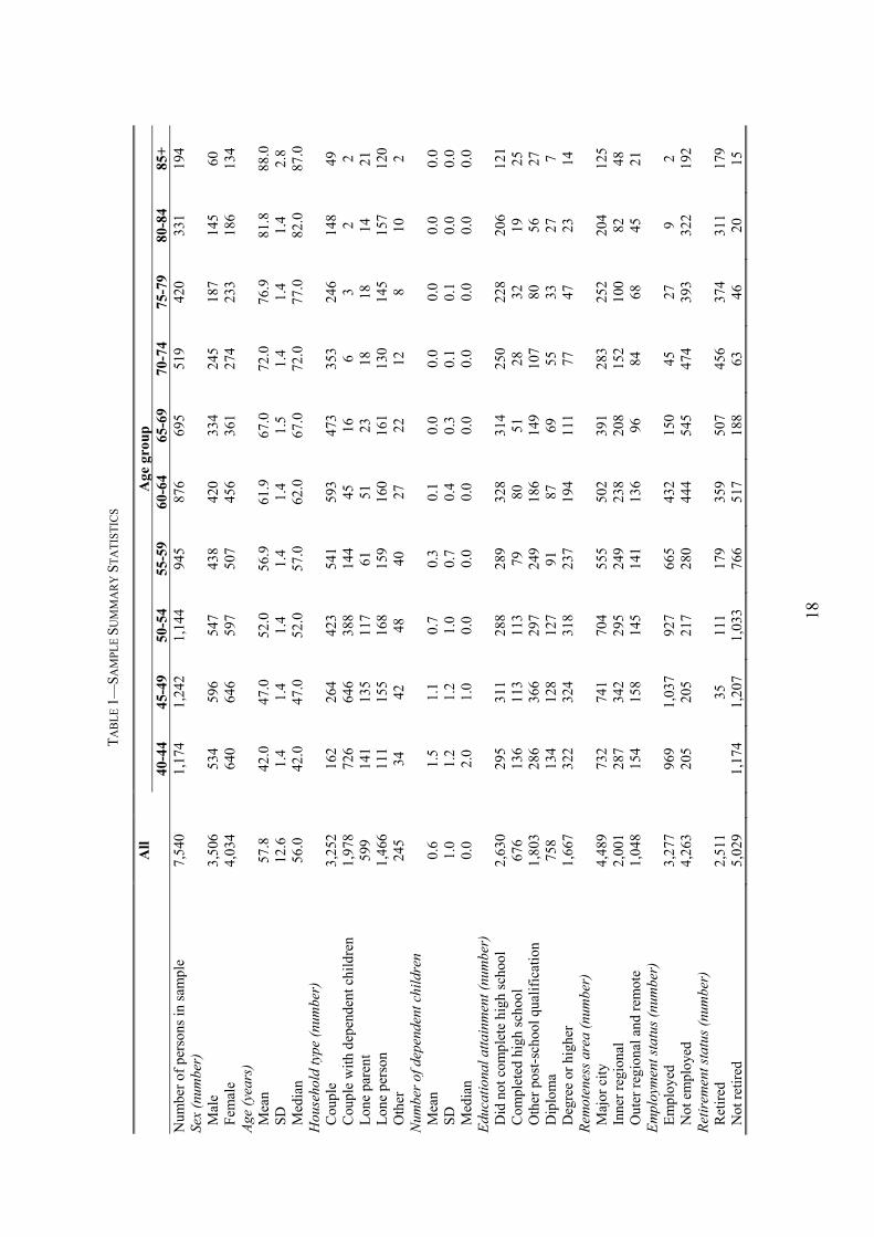
Table 1 provides statistics on the socio-demographic characteristics of our sample. The
7,540 individuals in our sample, of whom 4,034 (53.5 per cent) are female, reside in 5,001
households. The median and mean ages of our sample members are 56.0 years and 57.8 years,
respectively (standard deviation = 12.6). 5,230 (69.35 per cent) are married or live in a de-
facto marriage and 599 (7.95 per cent) are lone parents. The mean number of children is 0.6.
Of all sample members, 2,630 (34.95 per cent) did not complete high school, 676 (9.05 per
cent) completed high school, 2,561 (24.05 per cent) obtained other post-secondary school
qualification or a diploma, and 1,667 (22.15 per cent) have a university degree or higher
qualifications. 4,489 (59.55 per cent) sample members live in a major city, 2,001 (26.55 per
cent) live in inner regional Australia while 1,048 (13.95 per cent) live in remote areas. 3,277
(43.55 per cent) of our sample members are fully employed and 2,511 (33.35 per cent) are
9 This is also relevant for calculating pension amounts given the linking of the full pension to 25% of average weekly earnings.
16
fully retired from the workforce. A breakdown of demographic characteristics by age group is
provided in Table 1.
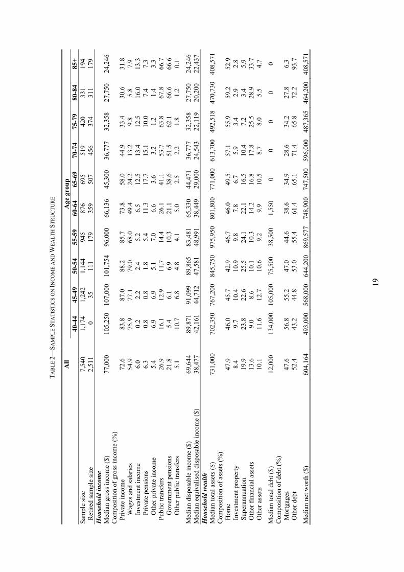
Table 2 provides sample summary statistics of income and wealth variables. Median gross
household income is $77,000 ($97,601 for sample members aged 40-64, and $34,880 for
sample members aged 65 and above).10 Private sources account for 72.6 per cent of gross
income received by sample members, although this share differs considerably be age group,
declining from 84 to 88 per cent among those aged 40 to 59 to approximately 30 per cent
among those aged 80 and over. The government pension is an important income source
among those aged 65 and over. Among sample members aged 65-69, government pensions
make up 39 per cent of income, rising up to two-thirds of income among sample members
aged 80 and above. In other words, the government pension is by far the most significant
source of retirement income.
Median household disposable income is $69,644 and declines in age from the 45-49 age
group onwards. Reflecting the effects of adult children moving out of the parental home,
median equalized household disposable income peaks later, reaching a high of $48,991 in the
55-59 age group age.11
Turning to household wealth, the median of total (gross) household assets in our sample is
$731,000. Median total assets peak in the 55-59 age group at $975,950, and thereafter
declines in age. The dominant asset class across all age groups in our sample is the home
(47.9 per cent of total assets), followed by retirement savings accounts (superannuation, 19.9
per cent), and other financial assets (13.6 per cent). In older age groups, retirement savings
accounts represent a much smaller share of total assets than in younger age groups, reflecting
the fact that superannuation was only introduced in 1992 and thus older members of our
sample did not contribute much to superannuation during their working lives. In addition,
older members will have drawn on those accounts during retirement. In those age groups,
other financial assets, mainly securities, are far more important.
10 All dollar figures are in Australian dollars at 2010 prices. The mean AUD/USD exchange rate in 2010 was 1.09. 11 Income is equivalised using the modified OECD scale, whereby household income is divided by the equivalence scale. The scale is equal to one plus 0.5 for each additional household member after the first aged 15 and over plus 0.3 for each child aged under 15. For details see A. Hagenaars, K. de Vos, M. Zaidi. 1994. "Poverty Statistics in the Late 1980s: Research Based on Micro-Data," Luxembourg: Office for Official Publications of the European Communities.
17
Median total household debt in the sample as a whole is $12,000, while median debt by age
group declines from $134,000 in the 40-44 age group down to 0 in all age groups above 65..
In younger households, debt is dominated by mortgages whereas older households’ debt is
mainly comprised of other forms of debt. Median net worth is $604,164. A breakdown of the
composition of income and wealth by age group is also provided in Table 2.
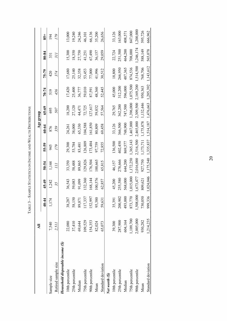
In Table 3 we provide statistics on the distributions of household disposable income and net
worth for the entire sample as well as by age group to demonstrate the high degree of
variability of income and wealth across the population. Looking at disposable income, the
ratio of the 90th percentile to the 10th percentile is 7.0 when taking into account the entire
sample. Across age groups, this ratio is largest in the age group 65 to 69 (7.0) and lowest in
the age group 40 to 44 (4.0). Disparities are even greater for net worth. Here, the ratio of the
90th percentile to the 10th percentile is 51.0 for the entire sample, highest in the age group 75
to 79 (80.6) and lowest in the age group 55 to 59 (18.4).
In summary, there is a high degree of heterogeneity in income and wealth across our sample
as well as in the composition of income and wealth. Thus, we expect there to be a
correspondingly high degree of heterogeneity in adequacy of retirement savings.
18
TA
BL
E 1
—SA
MPL
E S
UM
MA
RY
ST
AT
IST
ICS
A
ll
A
ge g
roup
40
-44
45-4
9 50
-54
55-5
9 60
-64
65-6
9 70
-74
75-7
9 80
-84
85+
N
umbe
r of
per
sons
in s
ampl
e 7,
540
1,
174
1,24
2 1,
144
945
876
695
519
420
331
194
Sex
(num
ber)
M
ale
3,50
6
534
596
547
438
420
334
245
187
145
60
Fem
ale
4,03
4
640
646
597
507
456
361
274
233
186
134
Age
(ye
ars)
M
ean
57.8
42.0
47
.0
52.0
56
.9
61.9
67
.0
72.0
76
.9
81.8
88
.0
SD
12
.6
1.
4 1.
4 1.
4 1.
4 1.
4 1.
5 1.
4 1.
4 1.
4 2.
8 M
edia
n 56
.0
42
.0
47.0
52
.0
57.0
62
.0
67.0
72
.0
77.0
82
.0
87.0
H
ouse
hold
type
(nu
mbe
r)
Cou
ple
3,25
2
162
264
423
541
593
473
353
246
148
49
Cou
ple
with
dep
ende
nt c
hild
ren
1,97
8
726
646
388
144
45
16
6 3
2 2
Lon
e pa
rent
59
9
141
135
117
61
51
23
18
18
14
21
Lon
e pe
rson
1,
466
11
1 15
5 16
8 15
9 16
0 16
1 13
0 14
5 15
7 12
0 O
ther
24
5
34
42
48
40
27
22
12
8 10
2
Num
ber
of d
epen
dent
chi
ldre
n
M
ean
0.6
1.
5 1.
1 0.
7 0.
3 0.
1 0.
0 0.
0 0.
0 0.
0 0.
0 S
D
1.0
1.
2 1.
2 1.
0 0.
7 0.
4 0.
3 0.
1 0.
1 0.
0 0.
0 M
edia
n 0.
0
2.0
1.0
0.0
0.0
0.0
0.0
0.0
0.0
0.0
0.0
Edu
catio
nal a
ttain
men
t (nu
mbe
r)
Did
not
com
plet
e hi
gh s
choo
l 2,
630
29
5 31
1 28
8 28
9 32
8 31
4 25
0 22
8 20
6 12
1 C
ompl
eted
hig
h sc
hool
67
6
136
113
113
79
80
51
28
32
19
25
Oth
er p
ost-
scho
ol q
ualif
icat
ion
1,80
3
286
366
297
249
186
149
107
80
56
27
Dip
lom
a 75
8
134
128
127
91
87
69
55
33
27
7 D
egre
e or
hig
her
1,66
7
322
324
318
237
194
111
77
47
23
14
Rem
oten
ess
area
(nu
mbe
r)
Maj
or c
ity
4,48
9
732
741
704
555
502
391
283
252
204
125
Inn
er r
egio
nal
2,00
1
287
342
295
249
238
208
152
100
82
48
Out
er r
egio
nal a
nd r
emot
e 1,
048
15
4 15
8 14
5 14
1 13
6 96
84
68
45
21
E
mpl
oym
ent s
tatu
s (n
umbe
r)
Em
ploy
ed
3,27
7
969
1,03
7 92
7 66
5 43
2 15
0 45
27
9
2 N
ot e
mpl
oyed
4,
263
20
5 20
5 21
7 28
0 44
4 54
5 47
4 39
3 32
2 19
2 R
etir
emen
t sta
tus
(num
ber)
R
etir
ed
2,51
1
35
11
1 17
9 35
9 50
7 45
6 37
4 31
1 17
9 N
ot r
etir
ed
5,02
9
1,17
4 1,
207
1,03
3 76
6 51
7 18
8 63
46
20
15
19
TA
BL
E 2
—SA
MPL
E S
TA
TIS
TIC
S O
N IN
CO
ME
AN
D W
EA
LT
H S
TR
UC
TU
RE
A
ll
A
ge g
roup
40
-44
45-4
9 50
-54
55-5
9 60
-64
65-6
9 70
-74
75-7
9 80
-84
85+
S
ampl
e si
ze
7,54
0
1,17
4 1,
242
1,14
4 94
5 87
6 69
5 51
9 42
0 33
1 19
4 R
etir
ed s
ampl
e si
ze
2,51
1
0
35
111
179
359
507
456
374
311
179
Hou
seho
ld in
com
e
M
edia
n gr
oss
inco
me
($)
77,0
00
10
5,25
0 10
7,00
0 10
1,75
4 96
,000
66
,136
45
,300
36
,777
32
,358
27
,750
24
,246
C
ompo
sitio
n of
gro
ss in
com
e (%
)
P
riva
te in
com
e 72
.6
83
.8
87.0
88
.2
85.7
73
.8
58.0
44
.9
33.4
30
.6
31.8
Wag
es a
nd s
alar
ies
54.9
75.9
77
.1
79.0
68
.0
49.4
24
.2
13.2
9.
8
5.8
7.
9
I
nves
tmen
t inc
ome
6.0
0.2
2.
2
2.4
5.
2
6.5
12
.5
13.4
12
.5
16.0
13
.3
P
riva
te p
ensi
ons
6.3
0.8
0.
8
1.8
5.
4
11.3
17
.7
15.1
10
.0
7.4
7.
3
O
ther
pri
vate
inco
me
5.4
6.9
6.
9
5.1
7.
0
6.6
3.
6
3.2
1.
2
1.4
3.
3
Pub
lic tr
ansf
ers
26.9
16.1
12
.9
11.7
14
.4
26.1
41
.1
53.7
63
.8
67.8
66
.7
G
over
nmen
t pen
sion
s 21
.8
5.
4
6.1
6.
9
10.3
21
.1
38.6
51
.5
62.1
66
.6
66.6
Oth
er p
ubli
c tr
ansf
ers
5.1
10.7
6.
8
4.8
4.
1
5.0
2.
5
2.2
1.
8
1.2
0.
1
Med
ian
disp
osab
le in
com
e ($
) 69
,644
89,8
71
91,0
99
89,8
65
83,4
81
65,3
30
44,4
71
36,7
77
32,3
58
27,7
50
24,2
46
Med
ian
equi
valis
ed d
ispo
sabl
e in
com
e ($
) 38
,477
42,1
61
44,7
12
47,5
81
48,9
91
38,4
49
29,0
00
24,5
43
22,1
19
20,2
00
22,4
37
Hou
seho
ld w
ealth
M
edia
n to
tal a
sset
s ($
) 73
1,00
0
702,
350
767,
200
845,
750
975,
950
801,
800
771,
000
613,
700
492,
518
470,
730
408,
571
Com
posi
tion
of a
sset
s (%
)
H
ome
47.9
46.0
45
.7
42.9
46
.7
46.0
49
.5
57.1
55
.9
59.2
52
.9
Inv
estm
ent p
rope
rty
8.
4
9.
7
10.4
10
.9
9.8
7.
8
6.7
5.
9
3.4
2.
9
2.8
S
uper
annu
atio
n 19
.9
23
.8
22.6
25
.5
24.1
22
.1
16.5
10
.4
7.2
3.
4
5.9
O
ther
fin
anci
al a
sset
s 13
.6
9.
0
8.6
10
.1
10.3
14
.2
16.8
17
.8
25.5
28
.9
33.7
O
ther
ass
ets
10.1
11.6
12
.7
10.6
9.
2
9.9
10
.5
8.7
8.
0
5.5
4.
7
Med
ian
tota
l deb
t ($)
12
,000
134,
000
105,
000
75,5
00
38,5
00
1,55
0 0
0 0
0 0
Com
posi
tion
of d
ebt (
%)
Mor
tgag
es
47.6
56.8
55
.2
47.0
44
.6
38.6
34
.9
28.6
34
.2
27.8
6.
3
Oth
er d
ebt
52.4
43.2
44
.8
53.0
55
.4
61.4
65
.1
71.4
65
.8
72.2
93
.7
Med
ian
net w
orth
($)
60
4,16
4
493,
000
568,
000
644,
200
869,
577
748,
900
747,
500
596,
000
487,
365
464,
200
408,
571
20
TA
BL
E 3
—SA
MPL
E S
TA
TIS
TIC
S O
N IN
CO
ME
AN
D W
EA
LT
H D
IST
RIB
UT
ION
S
All
Age
gro
up
40-4
4 45
-49
50-5
4 55
-59
60-6
4 65
-69
70-7
4 75
-79
80-8
4 85
+
Sam
ple
size
7,
540
1,
174
1,24
2 1,
144
945
876
695
519
420
331
194
Ret
ired
sam
ple
size
2,
511
35
111
179
359
507
456
374
311
179
Hou
seho
ld d
ispo
sabl
e in
com
e ($
)
10t
h pe
rcen
tile
22,0
80
38
,287
36
,543
33
,350
29
,300
24
,261
18
,200
17
,420
17
,680
15
,300
13
,000
25t
h pe
rcen
tile
37,4
10
58
,150
59
,083
58
,488
53
,784
38
,000
27
,120
25
,400
25
,140
18
,350
19
,240
Med
ian
69,6
44
89
,871
91
,099
89
,865
83
,481
65
,330
44
,471
36
,777
32
,358
27
,750
24
,246
75t
h pe
rcen
tile
109,
529
11
7,33
7 13
2,36
0 12
9,82
6 12
6,80
9 10
4,58
8 72
,725
59
,010
53
,453
41
,251
46
,101
90t
h pe
rcen
tile
154,
353
15
2,99
7 16
8,14
4 17
6,50
4 17
3,48
4 16
1,85
0 12
7,61
7 87
,591
77
,000
67
,490
66
,136
Mea
n 82
,024
95,3
80
100,
576
100,
665
97,7
59
80,8
09
59,8
32
48,3
60
41,9
96
36,1
57
35,2
00
Sta
ndar
d de
viat
ion
65,0
73
59
,631
62
,857
65
,815
72
,855
69
,458
57
,564
52
,445
30
,512
29
,059
26
,656
Net
wor
th (
$)
10t
h pe
rcen
tile
39,3
00
35
,391
45
,200
46
,157
13
6,50
0 33
,126
29
,765
45
,000
18
,800
22
,724
33
,126
25t
h pe
rcen
tile
287,
900
20
0,90
2 25
5,58
0 27
8,66
6 40
2,45
0 36
6,50
0 36
2,20
0 31
2,20
0 26
6,95
0 25
1,50
0 16
3,00
0
Med
ian
604,
164
49
3,00
0 56
8,00
0 64
4,20
0 86
9,57
7 74
8,90
0 74
7,50
0 59
6,00
0 48
7,36
5 46
4,20
0 40
8,57
1
75t
h pe
rcen
tile
1,10
9,70
0
873,
770
1,01
5,00
01,
172,
250
1,36
5,14
3 1,
467,
000
1,39
6,00
01,
075,
500
874,
536
708,
000
847,
000
90t
h pe
rcen
tile
2,00
5,00
0
1,50
8,00
01,
673,
477
2,01
6,00
02,
516,
500
2,46
5,00
02,
309,
500
2,16
9,20
01,
514,
500
1,24
6,17
41,
200,
000
Mea
n 93
0,28
2
730,
050
809,
621
927,
750
1,17
3,71
1 1,
175,
878
1,13
2,44
695
0,36
3 76
8,70
6 58
8,14
9 59
5,72
6
Sta
ndar
d de
viat
ion
1,21
4,23
5
999,
336
1,02
4,04
61,
175,
540
1,33
5,83
7 1,
514,
187
1,47
6,66
31,
205,
392
1,14
3,61
256
5,07
8 66
6,96
2
21
V. Results
We now combine the dataset in the previous section with our algorithm to calculate the
adequacy metrics described in Section III. In all of our analyses, we produce four alternative
projections of the consumption level in retirement, with each successive projection taking into
account one additional source (‘pillar’) of retirement income. The first projection considers
only compulsory retirement savings (compulsory superannuation). In the second projection
we add voluntary superannuation contributions, while the third projection additionally takes
into account the government pension (called the Age Pension in Australia). Finally, we add
other (net) savings to the pool of assets in the fourth projection. The latter information in
particular is typically not included in estimates of retirement savings due to unavailability of
data. To compute net savings, we add bank account balances, cash investments, equity
investments (net of investment loans), assets in trusts, life insurance contracts, property assets
(excluding the home, net of mortgages on those properties), and business assets (net of
business debt). The last projection, taking into account all pillars of retirement savings,
provides our primary set of results, while differences between the outcomes of the alternative
projections provide information on the relative contributions of the various pillars.
Consumption level and consumption shortfall
Consumption level
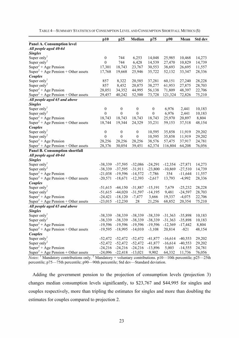
Figure 1 and Table 4 present summary statistics of our projections of consumption levels
during retirement as well as consumption shortfalls. Table 4 shows estimation results
separately for individuals below and above retirement age (65), and within those age groups
separately for singles and couples.12
We first look at consumption levels (Panel A of Table 4). In the age group 40 to 64, the
median consumption during retirement, only taking into account compulsory retirement
savings as a source of retirement income, is $6,253 per annum for singles and $20,585 per
annum for couples.13 The consumption level for singles is less than one third of the relative
poverty line in Australia (half of median equivalised disposable income in the population, and
equal to $19,990 in 2010). Couples are slightly better placed, but even their median
12 Age refers to an individual’s age in 2010. 13 All statistics reported in this section are population-weighted medians unless stated otherwise.
22
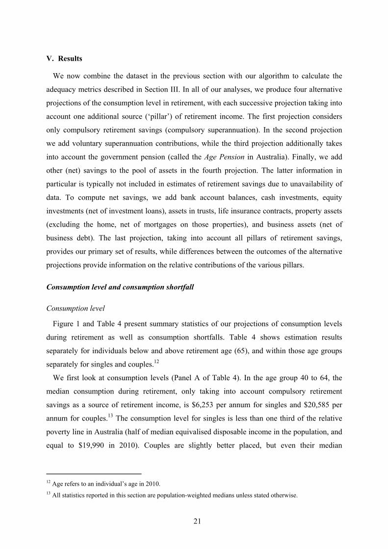
consumption levels are only about two-thirds of the relative poverty line. Taking into account
voluntary contributions to retirement savings accounts (projection 2) does not change
consumption levels materially, reflecting the fact that most people do not make significant
voluntary contributions.
FIGURE 1. CONSUMPTION SHORTFALL—AGES 40 TO 64
Notes: (A) Estimates of the consumption shortfall by projection basis and marital status. The metric is computed as the difference between the level of consumption that can be sustained until age 90 and the target level of consumption. In figure below, the target level of consumption is the ASFA ‘comfortable’ level deflated to 2010 prices ($38,339 for singles and $52,472 for couples). (B) Percentage of households expected to receive the Age Pension during retirement by projection. (C) Estimated percentage contribution of the Age Pension to household consumption during retirement, by projection.
99.5%
A. Estimates of consumption shortfall
Singles Couples
B. Percentage of HH receiving AP
C. Percentage contribution of age pension
-32,086(83.7%)
-31,887(60.8%)
-31,911(83.2%)
-31,597(60.2%)
-14,572(38.0%)
-7,477(14.2%)
-12,393(32.3%)
+28(0.0%)
Mandatorysuper
Mandatory +voluntary super
Mandatory +voluntary super +
age pension
Mandatory +voluntary super +
age pension +other assets
1 2 3 4
98.2% 95.8%
88.1%
74.6%
53.9%
66.7%
34.9%
1 2 3 4
1 2 3 4
Target
23
TABLE 4—SUMMARY STATISTICS OF CONSUMPTION LEVEL AND CONSUMPTION SHORTFALL METRICS ($)
p10 p25 Median p75 p90 Mean Std devPanel A. Consumption level All people aged 40-64 Singles Super only1 0 744 6,253 14,048 25,985 10,468 14,273 Super only2 0 744 6,428 14,539 27,470 10,829 14,739 Super2 + Age Pension 17,301 18,743 23,767 30,553 38,693 26,695 11,557 Super2 + Age Pension + Other assets 17,768 19,668 25,946 35,722 52,132 33,347 28,336 Couples Super only1 857 8,322 20,585 37,281 60,151 27,240 28,228 Super only2 857 8,452 20,875 38,277 61,953 27,875 28,703 Super2 + Age Pension 28,051 34,352 44,995 56,138 71,809 48,397 22,706 Super2 + Age Pension + Other assets 29,457 40,242 52,500 73,728 121,324 72,826 75,210 All people aged 65 and above Singles Super only1 0 0 0 0 6,976 2,441 10,183 Super only2 0 0 0 0 6,976 2,441 10,183 Super2 + Age Pension 18,743 18,743 18,743 18,743 25,970 20,897 8,804 Super2 + Age Pension + Other assets 18,744 19,344 24,329 35,231 59,153 37,518 48,154 Couples Super only1 0 0 0 10,595 35,858 11,919 29,202 Super only2 0 0 0 10,595 35,858 11,919 29,202 Super2 + Age Pension 28,256 28,256 28,256 38,576 57,475 37,917 24,781 Super2 + Age Pension + Other assets 28,376 30,054 39,451 62,374 116,804 64,208 76,056 Panel B. Consumption shortfall All people aged 40-64 Singles Super only1 -38,339 -37,595 -32,086 -24,291 -12,354 -27,871 14,273 Super only2 -38,339 -37,595 -31,911 -23,800 -10,869 -27,510 14,739 Super2 + Age Pension -21,038 -19,596 -14,572 -7,786 354 -11,644 11,557 Super2 + Age Pension + Other assets -20,571 -18,671 -12,393 -2,617 13,793 -4,992 28,336 Couples Super only1 -51,615 -44,150 -31,887 -15,191 7,679 -25,232 28,228 Super only2 -51,615 -44,020 -31,597 -14,195 9,481 -24,597 28,703 Super2 + Age Pension -24,421 -18,120 -7,477 3,666 19,337 -4,075 22,706 Super2 + Age Pension + Other assets -23,015 -12,230 28 21,256 68,852 20,354 75,210 All people aged 65 and above Singles Super only1 -38,339 -38,339 -38,339 -38,339 -31,363 -35,898 10,183 Super only2 -38,339 -38,339 -38,339 -38,339 -31,363 -35,898 10,183 Super2 + Age Pension -19,596 -19,596 -19,596 -19,596 -12,369 -17,442 8,804 Super2 + Age Pension + Other assets -19,595 -18,995 -14,010 -3,108 20,814 -821 48,154 Couples Super only1 -52,472 -52,472 -52,472 -41,877 -16,614 -40,553 29,202 Super only2 -52,472 -52,472 -52,472 -41,877 -16,614 -40,553 29,202 Super2 + Age Pension -24,216 -24,216 -24,216 -13,896 5,003 -14,555 24,781 Super2 + Age Pension + Other assets -24,096 -22,418 -13,021 9,902 64,332 11,736 76,056 Notes: 1 Mandatory contributions only. 2 Mandatory + voluntary contributions. p10—10th percentile; p25—25th percentile; p75—75th percentile; p90—90th percentile; Std dev—Standard deviation.
Adding the government pension to the projection of consumption levels (projection 3)
changes median consumption levels significantly, to $23,767 and $44,995 for singles and
couples respectively, more than tripling the estimates for singles and more than doubling the
estimates for couples compared to projection 2.
24
Adding other sources of retirement income increases the estimated median consumption
level to $25,946 for singles and $52,500 for couples, representing respective increases of 9.2
per cent and 16.7 per cent relative to the projections without these other sources. The
contribution of other sources increases with percentiles in the distribution. At the 90th
percentile of consumption levels, for example, the difference between projections 3 and 4 is
34.7 per cent for singles and 68.9 per cent for couples. This analysis shows that omitting
sources of retirement savings other than retirement savings accounts can lead to severe
underestimation of consumption levels in retirement.
Looking at the individuals aged 65 and above, we find that the estimated median
consumption level based on compulsory retirement savings alone is zero. This is unsurprising,
since compulsory contributions were only introduced when these individuals were 45 or
older. As a consequence, their lifetime compulsory contributions would be relatively low and,
for many in this age group, have already been exhausted by 2010 (when they were well into
their retirement). Their consumption is thus mainly funded by the government pension and
other retirement savings. In this group, the omission of other retirement savings has even
greater effects on the estimation of consumption levels. The difference between median
consumption levels in projections 3 and 4 is 29.8 per cent for singles and 39.6 per cent for
couples.
Consumption shortfall
Panel B of Table 4 presents our estimation results for the consumption shortfall metric. It
expresses estimated consumption levels in retirement relative to a benchmark consumption
level. As described in Section II, the benchmarks used in the present analysis are the ASFA
‘comfortable levels’, which are widely used in Australia as retirement income targets. These
levels are very similar to current mean income levels of retirees in Australia as well as to the
median level of retirement income deemed necessary by non-retired Australians for funding a
satisfactory lifestyle.
In our first projection, which takes into account compulsory retirement savings only, the
estimated median consumption shortfall in the age group 40-64 is $32,086 for singles and
$31,887 for couples, or 83.7 per cent and 60.8 per cent, respectively. It is therefore clear that,
for individuals in this age range, compulsory retirement savings are not yet nearly sufficient to
fund a comfortable level of consumption during retirement. Couples are, however, better-
placed than singles.
25
Adding the government pension substantially reduces the median consumption shortfall, to
$14,572 for singles (38.0 per cent below target) and $7,477 for couples (14.2 per cent below
target). Adding other retirement savings to the projections reduces the median shortfall
further, to $12,393 for singles (32.3 per cent below target) and to just below zero (-$28) for
couples. The shortfall for singles remains significant, however, even when taking all sources
of income into account.
Consumption shortfalls are substantially higher for individuals aged 65 and above. As noted
earlier, this population sub-group has almost no savings in compulsory retirement savings
accounts (superannuation) and largely depends on the Age Pension for their income. The
median consumption shortfall in projection 3 (retirement savings and government pension) is
$19,596 (51.1 per cent of target) for singles and $24,216 (63.2 per cent) for couples. Adding
other savings to the projections reduces the median shortfall to $14,010 (36.5 per cent) for
singles and $13,021 (34.0 per cent) for couples. It is worth noting that, while the consumption
shortfall is significantly larger for singles than for couples in the age group 40 to 64, this is
not the case in the group aged 65 and older.
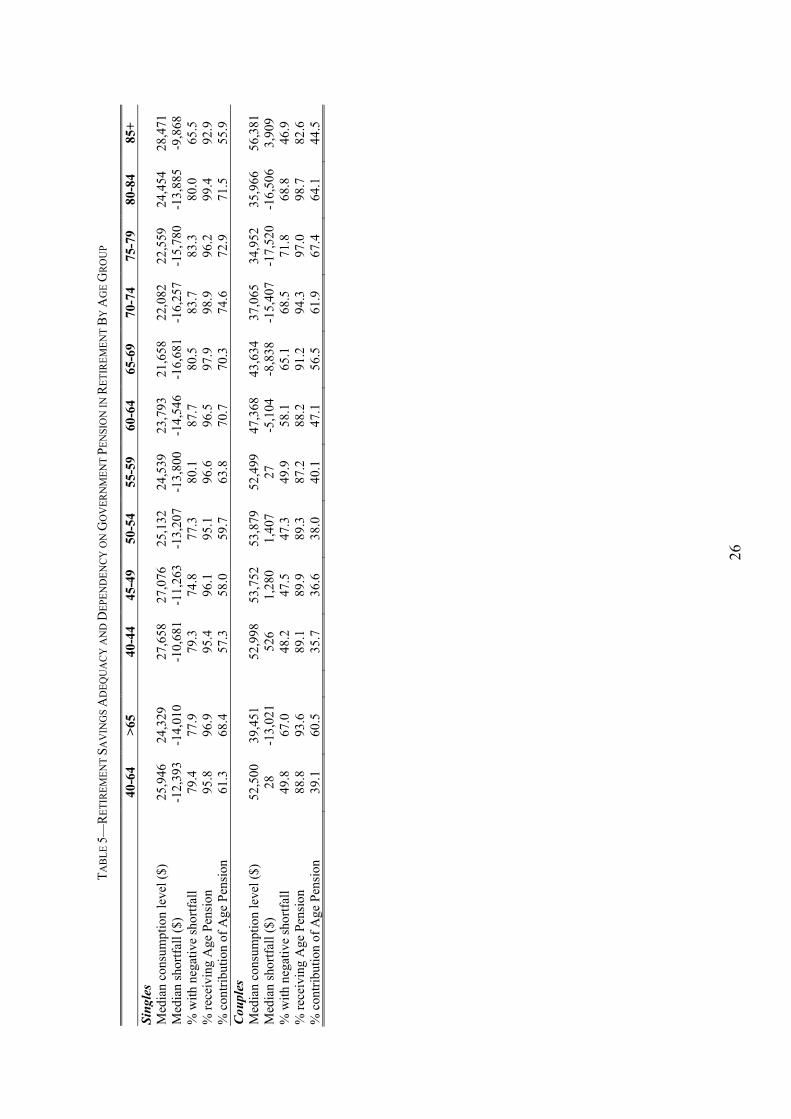
Table 5 presents statistics on consumption levels and shortfalls in projection 4 by age
group, as well as a set of measures indicating the level of dependency of retirees on the
government pension. For singles, the median consumption shortfall increases with age,
peaking in the age group 65 to 69. In the case of couples, there is no clear trend among the
younger age groups, while the consumption shortfall peaks in the age group 75 to 79.
Among those aged 40 to 64, the consumption shortfall is negative in 79.4 per cent of cases
for singles and 49.8 per cent of cases for couples; 95.8 per cent of singles are projected to
receive at least a partial government pension, which on average contributes 61.3 per cent of
their income; in the case of couples, 88.8 per cent are projected to receive the government
pension, which on average contributes 39.1 per cent to their income.
26
TA
BL
E 5
—R
ET
IRE
ME
NT
SA
VIN
GS
AD
EQ
UA
CY
AN
D D
EPE
ND
EN
CY
ON
GO
VE
RN
ME
NT
PE
NSI
ON
IN
RE
TIR
EM
EN
T B
Y A
GE
GR
OU
P
40
-64
>65
40-4
4 45
-49
50-5
4 55
-59
60-6
4 65
-69
70-7
4 75
-79
80-8
4 85
+
Sin
gles
Med
ian
cons
umpt
ion
leve
l ($)
25
,946
24
,329
27,6
58
27,0
76
25,1
32
24,5
39
23,7
93
21,6
58
22,0
82
22,5
59
24,4
54
28,4
71
Med
ian
shor
tfal
l ($)
-1
2,39
3 -1
4,01
0
-10,
681
-11,
263
-13,
207
-13,
800
-14,
546
-16,
681
-16,
257
-15,
780
-13,
885
-9,8
68
% w
ith n
egat
ive
shor
tfal
l 79
.4
77.9
79.3
74
.8
77.3
80
.1
87.7
80
.5
83.7
83
.3
80.0
65
.5
% r
ecei
ving
Age
Pen
sion
95
.8
96.9
95.4
96
.1
95.1
96
.6
96.5
97
.9
98.9
96
.2
99.4
92
.9
% c
ontr
ibut
ion
of A
ge P
ensi
on
61.3
68
.4
57
.3
58.0
59
.7
63.8
70
.7
70.3
74
.6
72.9
71
.5
55.9
C
oupl
es
M
edia
n co
nsum
ptio
n le
vel (
$)
52,5
00
39,4
51
52
,998
53
,752
53
,879
52
,499
47
,368
43
,634
37
,065
34
,952
35
,966
56
,381
M
edia
n sh
ortf
all (
$)
28
-13,
021
52
6 1,
280
1,40
7 27
-5
,104
-8
,838
-1
5,40
7 -1
7,52
0 -1
6,50
6 3,
909
% w
ith n
egat
ive
shor
tfal
l 49
.8
67.0
48.2
47
.5
47.3
49
.9
58.1
65
.1
68.5
71
.8
68.8
46
.9
% r
ecei
ving
Age
Pen
sion
88
.8
93.6
89.1
89
.9
89.3
87
.2
88.2
91
.2
94.3
97
.0
98.7
82
.6
% c
ontr
ibut
ion
of A
ge P
ensi
on
39.1
60
.5
35
.7
36.6
38
.0
40.1
47
.1
56.5
61
.9
67.4
64
.1
44.5
27
Comparing individuals aged 40 to 64 with individuals aged 65 and above, for singles there
is little difference in the consumption shortfall and in reliance on the government pension.
However, there are marked differences in the case of couples: the median consumption
shortfall is -$28 in the age group 40 to 64 and $13,021 in the age group 65 and older, while
the mean contribution of the government pension to income is 39.5 per cent in the age group
40 to 64 compared to 60.5 per cent in the age group 65 and older. A likely explanation for this
trend of decreasing reliance on the government pension is mandatory retirement savings.
Those in the age group 65 and older only contributed to superannuation for a small part of
their working lives, while those in the age group 40-64, and particularly the younger members
of this age group, contributed to superannuation for a significant part of their working lives.
Further analysis is required, however, to establish the causes of this difference across age
groups in dependency on the government pension.
Run-out age and age gap
We now turn to the second set of adequacy metrics, run-out age and age gap, presented in
Figure 2 and Table 6.
Run-out age
Panel A of Table 6 shows summary statistics for the run-out age metric. In the age group 40
to 64, the median run-out age is 69 years for singles in both projections 1 and 2 (compulsory
and voluntary superannuation), while for couples it is 75 years in projection 1 and 76 years in
projection 2. In projection 3 (including the government pension), the median run-out age does
not change for singles in the age group 40 to 64, but increases to 82 years for couples in the
same age group because eligibility for the government pension enables conservation of
private savings. Finally, in projection 4, the median run-out age is 71 years for singles in the
age group 40 to 64 and 92 years for couples. In most of our projections, the run-out age is
substantially below life expectancy, a point we turn to now.
Age gap
The age gap metric compares run-out age to life expectancy, given a member’s current age.
Panel B of Table 6 presents summary statistics for the age gap metric. In projection 1
(compulsory retirement savings only), singles in the age group 40 to 64 are expected to run
out of private retirement savings 20 years before life expectancy, compared to 13 years for
couples.
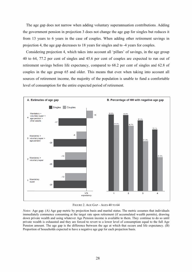
The a
the gove
from 13
projecti
Consi
40 to 6
retireme
couples
sources
level of
Notes: Agimmediatdown privprivate wPension aProportio
age gap doe
ernment pen
3 years to 6
on 4, the ag
idering proj
4, 77.2 per
ent savings
in the age
of retireme
f consumptio
ge gap. (A) Ately commencvate wealth an
wealth is exhauamount. The
on of househol
es not narrow
nsion in pro
6 years in
ge gap decre
jection 4, w
r cent of sin
before life
e group 65
ent income,
on for the e
Age gap metricce consuming nd using whausted and theage gap is thlds expected t
w when add
ojection 3 d
the case of
eases to 18 y
which takes
ngles and 4
e expectancy
and older.
, the majori
ntire expect
FIGURE 2. A
c by projectioat the target
tever Age Peny are forced te difference b
to have a nega
28
ding volunt
does not cha
f couples. W
years for sin
into accoun
45.6 per ce
y, compare
This mean
ity of the po
ted period o
AGE GAP – AG
on basis and mrate upon retnsion income to revert to a between the aative age gap f
tary superan
ange the age
When addin
ngles and to
nt all ‘pillar
ent of coupl
d to 68.2 p
ns that even
opulation is
of retiremen
GES 40 TO 64
marital status. irement (if acis available tlower level o
age at which for each proje
nnuation con
e gap for si
ng other ret
o -4 years fo
rs’ of saving
les are expe
per cent of
n when taki
s unable to
nt.
The metric accumulated weo them. They
of consumptiothat occurs anction basis.
ntributions.
ingles but re
tirement sa
or couples.
gs, in the ag
ected to ru
singles and
ing into acc
fund a com
assumes that inwealth permits)y continue to don equal to thend life expec
. Adding
educes it
avings in
ge group
un out of
d 62.8 of
count all
mfortable
ndividuals ), drawing do so until e full Age tancy. (B)
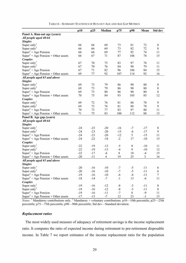
29
TABLE 6—SUMMARY STATISTICS OF RUN-OUT AGE AND AGE GAP METRICS
p10 p25 Median p75 p90 Mean Std devPanel A. Run-out age (years) All people aged 40-64 Singles Super only1 66 66 69 73 81 72 8 Super only2 66 66 69 73 82 72 8 Super2 + Age Pension 66 66 69 77 92 74 11 Super2 + Age Pension + Other assets 66 67 71 87 106 78 15 Couples Super only1 67 70 75 83 97 78 11 Super only2 67 70 76 84 98 79 11 Super2 + Age Pension 67 71 82 96 106 84 15 Super2 + Age Pension + Other assets 69 77 92 107 114 92 16 All people aged 65 and above Singles Super only1 69 73 79 86 90 80 8 Super only2 69 73 79 86 90 80 8 Super2 + Age Pension 69 73 80 86 90 80 8 Super2 + Age Pension + Other assets 70 75 84 93 105 85 12 Couples Super only1 69 72 76 81 88 78 9 Super only2 69 72 76 81 88 78 9 Super2 + Age Pension 70 73 77 83 97 80 11 Super2 + Age Pension + Other assets 71 75 83 100 112 88 15 Panel B. Age gap (years) All people aged 40-64 Singles Super only1 -24 -23 -20 -16 -7 -17 8 Super only2 -24 -23 -20 -15 -6 -17 9 Super2 + Age Pension -24 -23 -20 -12 5 -15 11 Super2 + Age Pension + Other assets -24 -22 -18 -2 17 -10 15 Couples Super only1 -22 -19 -13 -5 8 -10 11 Super only2 -22 -19 -13 -4 9 -10 12 Super2 + Age Pension -22 -17 -6 8 18 -4 15 Super2 + Age Pension + Other assets -20 -11 4 19 25 3 16 All people aged 65 and above Singles Super only1 -20 -16 -10 -7 -5 -11 6 Super only2 -20 -16 -10 -7 -5 -11 6 Super2 + Age Pension -19 -16 -10 -6 -4 -11 7 Super2 + Age Pension + Other assets -18 -14 -7 -1 13 -6 11 Couples Super only1 -19 -16 -12 -8 -3 -11 8 Super only2 -19 -16 -12 -8 -3 -11 8 Super2 + Age Pension -19 -16 -11 -7 8 -9 11 Super2 + Age Pension + Other assets -17 -13 -7 12 23 -1 15 Notes: 1 Mandatory contributions only. 2 Mandatory + voluntary contributions. p10—10th percentile; p25—25th percentile; p75—75th percentile; p90—90th percentile; Std dev—Standard deviation.
Replacement ratios
The most widely used measure of adequacy of retirement savings is the income replacement
ratio. It computes the ratio of expected income during retirement to pre-retirement disposable
income. In Table 7 we report estimates of the income replacement ratio for the population
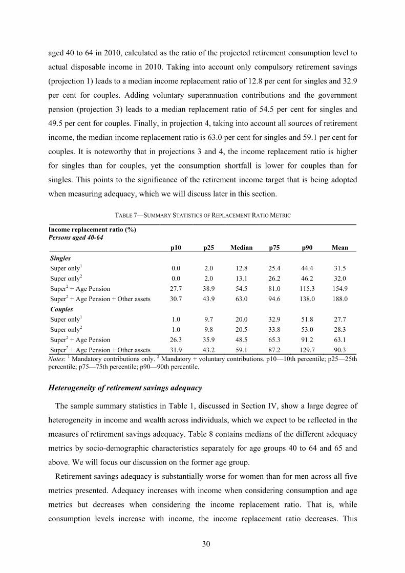
30
aged 40 to 64 in 2010, calculated as the ratio of the projected retirement consumption level to
actual disposable income in 2010. Taking into account only compulsory retirement savings
(projection 1) leads to a median income replacement ratio of 12.8 per cent for singles and 32.9
per cent for couples. Adding voluntary superannuation contributions and the government
pension (projection 3) leads to a median replacement ratio of 54.5 per cent for singles and
49.5 per cent for couples. Finally, in projection 4, taking into account all sources of retirement
income, the median income replacement ratio is 63.0 per cent for singles and 59.1 per cent for
couples. It is noteworthy that in projections 3 and 4, the income replacement ratio is higher
for singles than for couples, yet the consumption shortfall is lower for couples than for
singles. This points to the significance of the retirement income target that is being adopted
when measuring adequacy, which we will discuss later in this section.
TABLE 7—SUMMARY STATISTICS OF REPLACEMENT RATIO METRIC
Income replacement ratio (%) Persons aged 40-64
p10 p25 Median p75 p90 Mean
Singles
Super only1 0.0 2.0 12.8 25.4 44.4 31.5
Super only2 0.0 2.0 13.1 26.2 46.2 32.0
Super2 + Age Pension 27.7 38.9 54.5 81.0 115.3 154.9
Super2 + Age Pension + Other assets 30.7 43.9 63.0 94.6 138.0 188.0
Couples
Super only1 1.0 9.7 20.0 32.9 51.8 27.7
Super only2 1.0 9.8 20.5 33.8 53.0 28.3
Super2 + Age Pension 26.3 35.9 48.5 65.3 91.2 63.1
Super2 + Age Pension + Other assets 31.9 43.2 59.1 87.2 129.7 90.3 Notes: 1 Mandatory contributions only. 2 Mandatory + voluntary contributions. p10—10th percentile; p25—25th percentile; p75—75th percentile; p90—90th percentile.
Heterogeneity of retirement savings adequacy
The sample summary statistics in Table 1, discussed in Section IV, show a large degree of
heterogeneity in income and wealth across individuals, which we expect to be reflected in the
measures of retirement savings adequacy. Table 8 contains medians of the different adequacy
metrics by socio-demographic characteristics separately for age groups 40 to 64 and 65 and
above. We will focus our discussion on the former age group.
Retirement savings adequacy is substantially worse for women than for men across all five
metrics presented. Adequacy increases with income when considering consumption and age
metrics but decreases when considering the income replacement ratio. That is, while
consumption levels increase with income, the income replacement ratio decreases. This

31
relation is due to the fact that individuals with lower current income levels will be able to
achieve a higher replacement ratio than individuals with higher current income levels. The
main reason for this phenomenon is the government pension, which will replace a much larger
part of current income for low-income individuals. Thus, many low-income people with a
high projected income replacement ratio will nonetheless have low living standards in
retirement, while many high-income people with a low projected income replacement ratio
will nonetheless have relatively high living standards in retirement. This suggests that the
income replacement ratio has some shortcomings as an indicator of retirement savings
adequacy. The adequacy measure that is most appropriate depends on the goal of measuring
adequacy. If the goal is to measure adequacy against a fixed (universal) living standard, then
income replacement ratios are not appropriate. In such a case, it is more critical from a policy
perspective to assess whether people are meeting certain levels of living standards. However,
if the goal is to achieve a living standard that is closely related to the current standard of
living, then the income replacement ratio may be a more appropriate indicator.
As Table 8 shows, retirement savings adequacy improves with net worth. It is slightly
higher for couples with dependent children than for couples without children. This difference
is likely driven by higher income and wealth in the former group. Adequacy is lower for lone
parents than for lone persons. Adequacy increases with the number of children until two and
then decreases, and is lowest for households with four or more children. Adequacy also
increases with educational attainment and decreases with remoteness of residence. It is
substantially lower for the non-employed than the employed, and significantly lower for
individuals who have already retired than for those who have not yet retired.
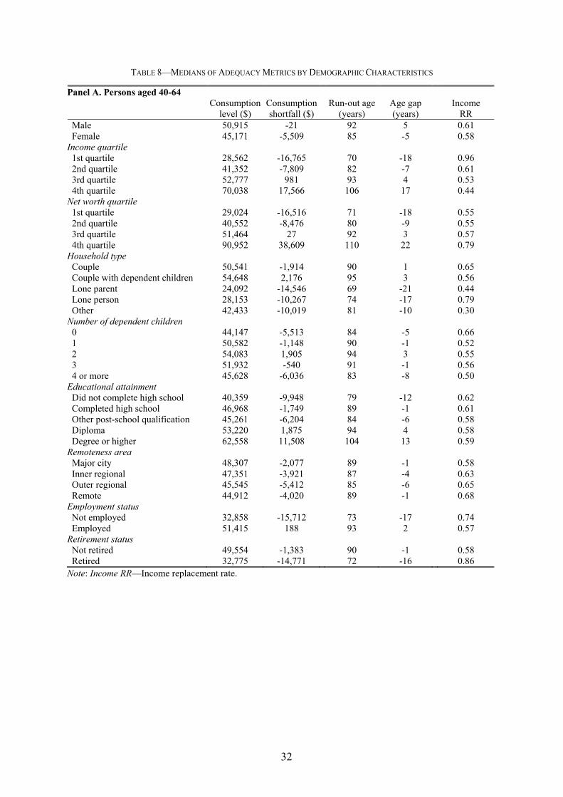
32
TABLE 8—MEDIANS OF ADEQUACY METRICS BY DEMOGRAPHIC CHARACTERISTICS
Panel A. Persons aged 40-64 Consumption
level ($) Consumption shortfall ($)
Run-out age (years)
Age gap (years)
Income RR
Male 50,915 -21 92 5 0.61 Female 45,171 -5,509 85 -5 0.58
Income quartile 1st quartile 28,562 -16,765 70 -18 0.96 2nd quartile 41,352 -7,809 82 -7 0.61 3rd quartile 52,777 981 93 4 0.53 4th quartile 70,038 17,566 106 17 0.44
Net worth quartile 1st quartile 29,024 -16,516 71 -18 0.55 2nd quartile 40,552 -8,476 80 -9 0.55 3rd quartile 51,464 27 92 3 0.57 4th quartile 90,952 38,609 110 22 0.79
Household type Couple 50,541 -1,914 90 1 0.65 Couple with dependent children 54,648 2,176 95 3 0.56 Lone parent 24,092 -14,546 69 -21 0.44 Lone person 28,153 -10,267 74 -17 0.79 Other 42,433 -10,019 81 -10 0.30
Number of dependent children 0 44,147 -5,513 84 -5 0.66 1 50,582 -1,148 90 -1 0.52 2 54,083 1,905 94 3 0.55 3 51,932 -540 91 -1 0.56 4 or more 45,628 -6,036 83 -8 0.50
Educational attainment Did not complete high school 40,359 -9,948 79 -12 0.62 Completed high school 46,968 -1,749 89 -1 0.61 Other post-school qualification 45,261 -6,204 84 -6 0.58 Diploma 53,220 1,875 94 4 0.58 Degree or higher 62,558 11,508 104 13 0.59
Remoteness area Major city 48,307 -2,077 89 -1 0.58 Inner regional 47,351 -3,921 87 -4 0.63 Outer regional 45,545 -5,412 85 -6 0.65 Remote 44,912 -4,020 89 -1 0.68
Employment status Not employed 32,858 -15,712 73 -17 0.74 Employed 51,415 188 93 2 0.57
Retirement status Not retired 49,554 -1,383 90 -1 0.58 Retired 32,775 -14,771 72 -16 0.86
Note: Income RR—Income replacement rate.
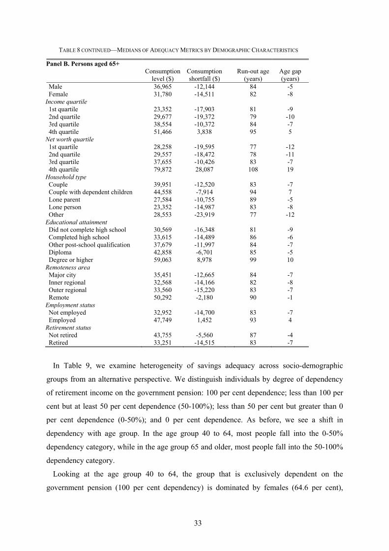
33
TABLE 8 CONTINUED—MEDIANS OF ADEQUACY METRICS BY DEMOGRAPHIC CHARACTERISTICS
Panel B. Persons aged 65+ Consumption
level ($) Consumption shortfall ($)
Run-out age (years)
Age gap (years)
Male 36,965 -12,144 84 -5 Female 31,780 -14,511 82 -8
Income quartile 1st quartile 23,352 -17,903 81 -9 2nd quartile 29,677 -19,372 79 -10 3rd quartile 38,554 -10,372 84 -7 4th quartile 51,466 3,838 95 5
Net worth quartile 1st quartile 28,258 -19,595 77 -12 2nd quartile 29,557 -18,472 78 -11 3rd quartile 37,655 -10,426 83 -7 4th quartile 79,872 28,087 108 19
Household type Couple 39,951 -12,520 83 -7 Couple with dependent children 44,558 -7,914 94 7 Lone parent 27,584 -10,755 89 -5 Lone person 23,352 -14,987 83 -8 Other 28,553 -23,919 77 -12
Educational attainment Did not complete high school 30,569 -16,348 81 -9 Completed high school 33,615 -14,489 86 -6 Other post-school qualification 37,679 -11,997 84 -7 Diploma 42,858 -6,701 85 -5 Degree or higher 59,063 8,978 99 10
Remoteness area Major city 35,451 -12,665 84 -7 Inner regional 32,568 -14,166 82 -8 Outer regional 33,560 -15,220 83 -7 Remote 50,292 -2,180 90 -1
Employment status Not employed 32,952 -14,700 83 -7 Employed 47,749 1,452 93 4
Retirement status Not retired 43,755 -5,560 87 -4 Retired 33,251 -14,515 83 -7
In Table 9, we examine heterogeneity of savings adequacy across socio-demographic
groups from an alternative perspective. We distinguish individuals by degree of dependency
of retirement income on the government pension: 100 per cent dependence; less than 100 per
cent but at least 50 per cent dependence (50-100%); less than 50 per cent but greater than 0
per cent dependence (0-50%); and 0 per cent dependence. As before, we see a shift in
dependency with age group. In the age group 40 to 64, most people fall into the 0-50%
dependency category, while in the age group 65 and older, most people fall into the 50-100%
dependency category.
Looking at the age group 40 to 64, the group that is exclusively dependent on the
government pension (100 per cent dependency) is dominated by females (64.6 per cent),
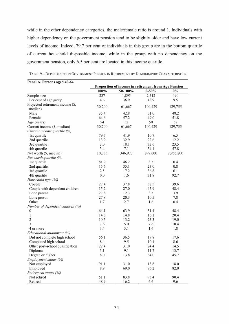
34
while in the other dependency categories, the male/female ratio is around 1. Individuals with
higher dependency on the government pension tend to be slightly older and have low current
levels of income. Indeed, 79.7 per cent of individuals in this group are in the bottom quartile
of current household disposable income, while in the group with no dependency on the
government pension, only 6.5 per cent are located in this income quartile.
TABLE 9—DEPENDENCY ON GOVERNMENT PENSION IN RETIREMENT BY DEMOGRAPHIC CHARACTERISTICS
Panel A. Persons aged 40-64 Proportion of income in retirement from Age Pension
100% 50-100% 0-50% 0% Sample size 237 1,895 2,512 490 Per cent of age group 4.6 36.9 48.9 9.5
Projected retirement income ($, median)
30,200 61,667 104,429 129,755
Male 35.4 42.8 51.0 48.2 Female 64.6 57.2 49.0 51.8
Age (years) 54 52 50 52 Current income ($, median) 30,200 61,667 104,429 129,755 Current income quartile (%) 1st quartile 79.7 41.9 10.7 6.5 2nd quartile 13.9 32.9 22.6 12.2 3rd quartile 3.0 18.1 32.6 23.5 4th quartile 3.4 7.1 34.1 57.8
Net worth ($, median) 10,335 346,973 897,000 2,956,800 Net worth quartile (%) 1st quartile 81.9 46.2 8.5 0.4 2nd quartile 15.6 35.1 23.0 0.8 3rd quartile 2.5 17.2 36.8 6.1 4th quartile 0.0 1.6 31.8 92.7
Household type (%) Couple 27.4 37.8 38.5 39.6 Couple with dependent children 15.2 27.0 45.9 48.4 Lone parent 27.8 12.3 3.5 3.9 Lone person 27.8 20.3 10.5 7.8 Other 1.7 2.7 1.6 0.4
Number of dependent children (%) 0 64.1 63.9 51.4 48.4 1 14.3 14.8 16.1 20.4 2 10.5 13.2 23.3 19.0 3 7.6 5.0 7.6 10.4 4 or more 3.4 3.1 1.6 1.8
Educational attainment (%) Did not complete high school 56.1 36.5 19.8 17.6 Completed high school 8.4 9.5 10.1 8.6 Other post-school qualification 22.4 31.0 24.4 14.5 Diploma 5.1 9.1 11.7 13.7 Degree or higher 8.0 13.8 34.0 45.7
Employment status (%) Not employed 91.1 31.0 13.8 18.0 Employed 8.9 69.0 86.2 82.0
Retirement status (%) Not retired 51.1 83.8 93.4 90.4 Retired 48.9 16.2 6.6 9.6
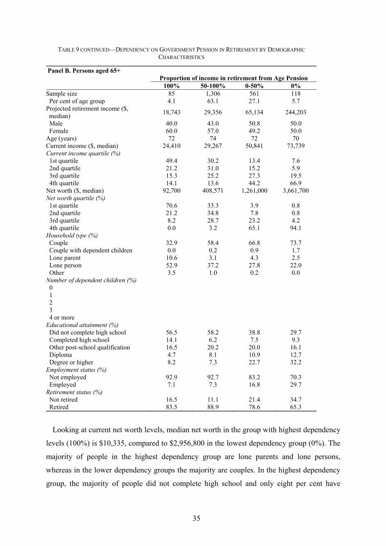
35
TABLE 9 CONTINUED—DEPENDENCY ON GOVERNMENT PENSION IN RETIREMENT BY DEMOGRAPHIC
CHARACTERISTICS
Panel B. Persons aged 65+ Proportion of income in retirement from Age Pension
100% 50-100% 0-50% 0% Sample size 85 1,306 561 118 Per cent of age group 4.1 63.1 27.1 5.7
Projected retirement income ($, median)
18,743 29,356 65,134 244,203
Male 40.0 43.0 50.8 50.0 Female 60.0 57.0 49.2 50.0
Age (years) 72 74 72 70 Current income ($, median) 24,410 29,267 50,841 73,739 Current income quartile (%) 1st quartile 49.4 30.2 13.4 7.6 2nd quartile 21.2 31.0 15.2 5.9 3rd quartile 15.3 25.2 27.3 19.5 4th quartile 14.1 13.6 44.2 66.9
Net worth ($, median) 92,700 408,571 1,261,000 3,661,700 Net worth quartile (%) 1st quartile 70.6 33.3 3.9 0.8 2nd quartile 21.2 34.8 7.8 0.8 3rd quartile 8.2 28.7 23.2 4.2 4th quartile 0.0 3.2 65.1 94.1
Household type (%) Couple 32.9 58.4 66.8 73.7 Couple with dependent children 0.0 0.2 0.9 1.7 Lone parent 10.6 3.1 4.3 2.5 Lone person 52.9 37.2 27.8 22.0 Other 3.5 1.0 0.2 0.0
Number of dependent children (%) 0 1 2 3 4 or more
Educational attainment (%) Did not complete high school 56.5 58.2 38.8 29.7 Completed high school 14.1 6.2 7.5 9.3 Other post-school qualification 16.5 20.2 20.0 16.1 Diploma 4.7 8.1 10.9 12.7 Degree or higher 8.2 7.3 22.7 32.2
Employment status (%) Not employed 92.9 92.7 83.2 70.3 Employed 7.1 7.3 16.8 29.7
Retirement status (%) Not retired 16.5 11.1 21.4 34.7 Retired 83.5 88.9 78.6 65.3
Looking at current net worth levels, median net worth in the group with highest dependency
levels (100%) is $10,335, compared to $2,956,800 in the lowest dependency group (0%). The
majority of people in the highest dependency group are lone parents and lone persons,
whereas in the lower dependency groups the majority are couples. In the highest dependency
group, the majority of people did not complete high school and only eight per cent have
36
university degrees, whereas in the lowest dependency group 45.7 per cent have university
degrees and only 17.6 per cent did not complete high school. 91.1 per cent in the highest
dependency group are unemployed and 48.9 per cent are retired, whereas in the lowest
dependency group only 18 per cent are not employed and 9.6 per cent are retired.
Relationship between adequacy metrics and other financial indicators
In Table 10, we consider the relationship between the different adequacy metrics across the
four projections as well as the relationship between these metrics and key financial figures,
using Spearman rank correlations, with the aim to see to what extent key financial figures
proxy for adequacy. All correlations reported are significant at the p<0.001 level.
We first look at correlations of the same adequacy metric across the four projections
considered above. Table 10 shows that correlations of the consumption shortfall metrics
across the first three projections are all above 0.9, indicating that the metric in those three
projections conveys about the same amount information. However, the correlation between
the consumption shortfall in the first three projections and the consumption shortfall in
projection four is significantly lower. For example, it is 0.7256 between projection 3 and
projection 4. This lower correlation indicates that the addition of other assets to the estimation
of retirement saving adequacy adds a significant amount of information, as indicated by
earlier analyses. The correlations in the age gap metric across the four projections exhibit a
similar pattern and therefore lead to a similar conclusion.
To compare the ordering of individuals across the two metrics, we examined the correlation
between the projection 4 consumption shortfall metric and the projection 4 age gap metric.
This was found to equal 0.971, implying the two metrics provide very similar predictions, and
suggesting that the choice between them for provision of information to individuals about
retirement savings adequacy is likely to depend on behavioral considerations.14
14 It is important to note, however, that the behavior assumed in the estimations of the age gap does not maximize Age Pension receipts.
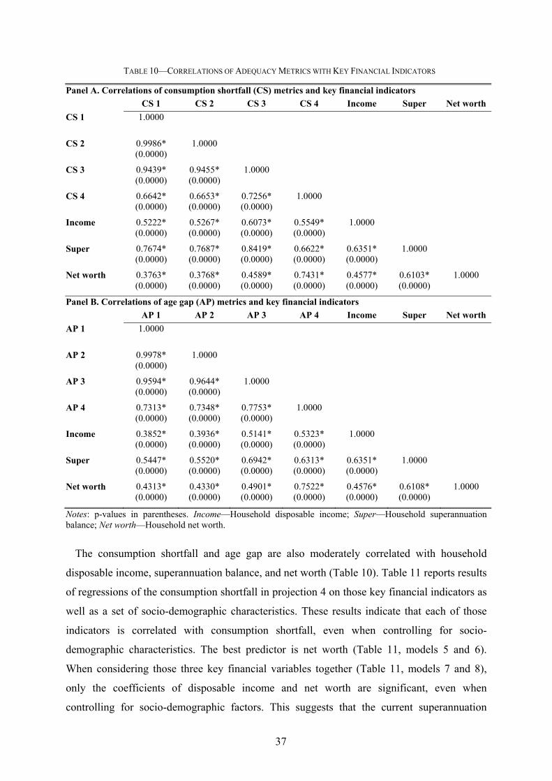
37
TABLE 10—CORRELATIONS OF ADEQUACY METRICS WITH KEY FINANCIAL INDICATORS
Panel A. Correlations of consumption shortfall (CS) metrics and key financial indicators
CS 1 CS 2 CS 3 CS 4 Income Super Net worth
CS 1 1.0000
CS 2 0.9986* (0.0000)
1.0000
CS 3 0.9439* (0.0000)
0.9455* (0.0000)
1.0000
CS 4 0.6642* (0.0000)
0.6653* (0.0000)
0.7256* (0.0000)
1.0000
Income 0.5222* (0.0000)
0.5267* (0.0000)
0.6073* (0.0000)
0.5549* (0.0000)
1.0000
Super 0.7674* (0.0000)
0.7687* (0.0000)
0.8419* (0.0000)
0.6622* (0.0000)
0.6351* (0.0000)
1.0000
Net worth 0.3763* (0.0000)
0.3768* (0.0000)
0.4589* (0.0000)
0.7431* (0.0000)
0.4577* (0.0000)
0.6103* (0.0000)
1.0000
Panel B. Correlations of age gap (AP) metrics and key financial indicators
AP 1 AP 2 AP 3 AP 4 Income Super Net worth
AP 1 1.0000
AP 2 0.9978* (0.0000)
1.0000
AP 3 0.9594* (0.0000)
0.9644* (0.0000)
1.0000
AP 4 0.7313* (0.0000)
0.7348* (0.0000)
0.7753* (0.0000)
1.0000
Income 0.3852* (0.0000)
0.3936* (0.0000)
0.5141* (0.0000)
0.5323* (0.0000)
1.0000
Super 0.5447* (0.0000)
0.5520* (0.0000)
0.6942* (0.0000)
0.6313* (0.0000)
0.6351* (0.0000)
1.0000
Net worth 0.4313* (0.0000)
0.4330* (0.0000)
0.4901* (0.0000)
0.7522* (0.0000)
0.4576* (0.0000)
0.6108* (0.0000)
1.0000
Notes: p-values in parentheses. Income—Household disposable income; Super—Household superannuation balance; Net worth—Household net worth.
The consumption shortfall and age gap are also moderately correlated with household
disposable income, superannuation balance, and net worth (Table 10). Table 11 reports results
of regressions of the consumption shortfall in projection 4 on those key financial indicators as
well as a set of socio-demographic characteristics. These results indicate that each of those
indicators is correlated with consumption shortfall, even when controlling for socio-
demographic characteristics. The best predictor is net worth (Table 11, models 5 and 6).
When considering those three key financial variables together (Table 11, models 7 and 8),
only the coefficients of disposable income and net worth are significant, even when
controlling for socio-demographic factors. This suggests that the current superannuation
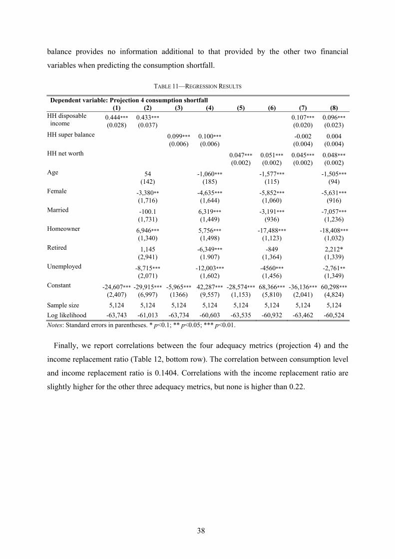
38
balance provides no information additional to that provided by the other two financial
variables when predicting the consumption shortfall.
TABLE 11—REGRESSION RESULTS
Dependent variable: Projection 4 consumption shortfall (1) (2) (3) (4) (5) (6) (7) (8) HH disposable income
0.444*** (0.028)
0.433*** (0.037)
0.107*** (0.020)
0.096*** (0.023)
HH super balance
0.099*** (0.006)
0.100*** (0.006)
-0.002 (0.004)
0.004 (0.004)
HH net worth
0.047*** (0.002)
0.051*** (0.002)
0.045*** (0.002)
0.048*** (0.002)
Age
54 (142)
-1,060***
(185)
-1,577*** (115)
-1,505***
(94)
Female
-3,380** (1,716)
-4,635***
(1,644)
-5,852*** (1,060)
-5,631***
(916)
Married
-100.1 (1,731)
6,319*** (1,449)
-3,191*** (936)
-7,057***
(1,236)
Homeowner
6,946*** (1,340)
5,756*** (1,498)
-17,488*** (1,123)
-18,408***
(1,032)
Retired
1,145 (2,941)
-6,349***
(1.907)
-849 (1,364)
2,212* (1,339)
Unemployed
-8,715*** (2,071)
-12,003***
(1,602)
-4560*** (1,456)
-2,761** (1,349)
Constant -24,607*** (2,407)
-29,915*** (6,997)
-5,965***
(1366) 42,287***
(9,557) -28,574***
(1,153) 68,366***
(5,810) -36,136***
(2,041) 60,298***
(4,824)
Sample size 5,124 5,124 5,124 5,124 5,124 5,124 5,124 5,124
Log likelihood -63,743 -61,013 -63,734 -60,603 -63,535 -60,932 -63,462 -60,524
Notes: Standard errors in parentheses. * p<0.1; ** p<0.05; *** p<0.01.
Finally, we report correlations between the four adequacy metrics (projection 4) and the
income replacement ratio (Table 12, bottom row). The correlation between consumption level
and income replacement ratio is 0.1404. Correlations with the income replacement ratio are
slightly higher for the other three adequacy metrics, but none is higher than 0.22.
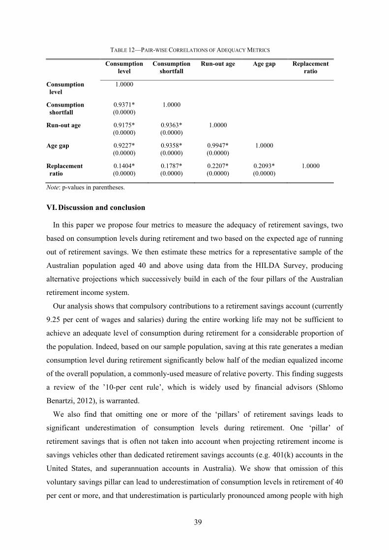
39
TABLE 12—PAIR-WISE CORRELATIONS OF ADEQUACY METRICS
Consumption level
Consumption shortfall
Run-out age Age gap Replacement ratio
Consumption level
1.0000
Consumption shortfall
0.9371* (0.0000)
1.0000
Run-out age 0.9175* (0.0000)
0.9363* (0.0000)
1.0000
Age gap 0.9227* (0.0000)
0.9358* (0.0000)
0.9947* (0.0000)
1.0000
Replacement ratio
0.1404* (0.0000)
0.1787* (0.0000)
0.2207* (0.0000)
0.2093* (0.0000)
1.0000
Note: p-values in parentheses.
VI. Discussion and conclusion
In this paper we propose four metrics to measure the adequacy of retirement savings, two
based on consumption levels during retirement and two based on the expected age of running
out of retirement savings. We then estimate these metrics for a representative sample of the
Australian population aged 40 and above using data from the HILDA Survey, producing
alternative projections which successively build in each of the four pillars of the Australian
retirement income system.
Our analysis shows that compulsory contributions to a retirement savings account (currently
9.25 per cent of wages and salaries) during the entire working life may not be sufficient to
achieve an adequate level of consumption during retirement for a considerable proportion of
the population. Indeed, based on our sample population, saving at this rate generates a median
consumption level during retirement significantly below half of the median equalized income
of the overall population, a commonly-used measure of relative poverty. This finding suggests
a review of the ’10-per cent rule’, which is widely used by financial advisors (Shlomo
Benartzi, 2012), is warranted.
We also find that omitting one or more of the ‘pillars’ of retirement savings leads to
significant underestimation of consumption levels during retirement. One ‘pillar’ of
retirement savings that is often not taken into account when projecting retirement income is
savings vehicles other than dedicated retirement savings accounts (e.g. 401(k) accounts in the
United States, and superannuation accounts in Australia). We show that omission of this
voluntary savings pillar can lead to underestimation of consumption levels in retirement of 40
per cent or more, and that underestimation is particularly pronounced among people with high
40
expected levels of consumption. We conclude from this part of the analysis that assessment of
the adequacy of retirement savings should take into account all sources of retirement income
and not just dedicated retirement savings accounts and social security payments, as is often
the case.
As our analyses make clear, the introduction of compulsory retirement savings seems to
have reduced the relative contribution of the government pension to retirement income while
increasing the contribution of (largely defined-contribution) retirement savings accounts. This
means that the proportion of consumption from potentially risky assets, in particular
retirement savings accounts, is increasing. This has implications for optimal portfolio
allocation and suggests that portfolio allocation too needs to take into account all sources of
retirement income, in particular government pensions, property and other assets, rather than
focus in isolation on (a particular set of) retirement savings accounts such as 401(k) accounts
in the United States or their equivalents elsewhere (Justin Wood, 2013). At the same, it also
suggests that it is important to take into account risk when projecting adequacy of retirement
savings, which is the subject of ongoing and planned future work by the authors.
We also report large heterogeneity in the adequacy of retirement savings across the
population. This finding suggests that a ‘one-size-fits-all’ approach to retirement savings is
likely to be inappropriate and that more personalized approaches should be pursued, taking
into account individual circumstances.
A further key finding is the high correlations between our adequacy metrics on the one
hand, and the low correlations between those metrics and the income replacement ratio on the
other. Most importantly, the income replacement ratio tends to be higher for low-income
groups and lower for high-income groups, while projected consumption levels in retirement
are higher for the latter group than for the former. We conclude that the assessment of savings
adequacy should at least be supplemented by the kind of metrics we propose.
We also find that financial variables such as current household income, superannuation
balance and net worth are not necessarily good ‘proxies’ for measures of adequacy of
retirement savings. In other words, the position of individuals in the distributions of current
household income, superannuation balance and net worth are not necessarily good reflections
of their positions in the distribution of retirement adequacy.
The projection of consumption levels during retirement of course depends on a large set of
assumptions about individual, household and market factors, including wages, salaries and
other income across the life cycle, real wage growth, employment status, marital status, home
ownership status, retirement age as well as asset returns and their temporal patterns. We keep
41
all of the factors constant in the projections presented in this article to focus on the
presentation of a new set of adequacy metrics and the assessment of the relative contributions
of the four ‘pillars’ of retirement savings. An important direction of research in this area is the
introduction into the model of uncertainty about the factors influencing adequacy, particularly
stochastic asset returns and the impact of planned or involuntary retirement at different ages,
and the investigation of the sensitivity of adequacy metrics to changes in the factors
influencing retirement adequacy.
Finally, we also report significant gaps between the level of income individuals expect to
need during retirement for a satisfactory lifestyle and their projected income in retirement.
While the HILDA Survey data does not contain information about individuals’ own
assessments of the adequacy of their retirement savings, other studies report that a large
fraction of the population acknowledge that they are not saving enough and would like to save
more (G. D. Carroll et al., 2009). We believe that one means to help close the retirement
savings gap is the provision of easily accessible tools, such as online retirement savings
calculators or ‘financial health checks’, that help people assess the adequacy of their own
retirement savings using metrics like the ones we present in this article.15 Information
provision of this sort is potentially one important addition to other measures to promote
retirement savings, such as tax incentives, reducing pension eligibility (for example, by
increasing the minimum age of eligibility), and the promotion of appropriate investment
strategies. However, the efficacy of various mechanisms such as these is an unresolved
empirical question, and warrants further investigation.
15 For an example see the calculators at http://www.moneysmart.com.au, a website about personal finance maintained by the Australian Securities and Investment Commission, the Australian regulatory agency for consumer finance and financial markets.
42
REFERENCES
A. Hagenaars, K. de Vos, M. Zaidi. 1994. "Poverty Statistics in the Late 1980s: Research Based on Micro-Data," Luxembourg: Office for Official Publications of the European Communities.
Australian Bureau of Statistics. 2013. "Australian Demographic Statistics, June 2013," ABS Catalogue No. 3101.0, Time Series Spreadsheets.
Basu, A. and M. Drew. 2010. "The Appropriateness of Default Investment Options in Defined Contribution Plans: Australian Evidence." Pacific Basin Financial Journal, 18(3), 290-305.
Benartzi, Shlomo. 2012. Save More Tomorrow: Practical Behavioral Finance Solutions to Improve 401(K). New York, NY: Penguin Group.
Bernheim, B. Douglas. 1992. "Is the Baby Boom Generation Preparing Adequately for Retirement?," Merrill Lynch.
Bernheim, B. Douglas and Antonio Rangel. 2005. "Behavioral Public Economics: Welfare and Policy Analysis with Non-Standard Decision-Makers," National Bureau of Economic Research.
Bernheim, B. Douglas; Jonathan Skinner and Stephen Weinberg. 2001. "What Accounts for the Variation in Retirement Wealth among Us Households?" American Economic Review, 91(4), 832-57.
Beshears, J.; J. J. Choi; D. Laibson and B. C. Madrian. 2009. "The Importance of Default Options for Retirement Savings Outcomes: Evidence from the United States," J. Brown, Social Security Policy in a Changing World. Chicago: University of Chicago Press.
Booth, P. and Y. Yakoubov. 2000. "Investment Policy for Defined-Contribution Pension Scheme Members Close to Retirement: An Analysis of the “Lifestyle” Concept." North American Actuarial Journal, 4, 1-19.
Carroll, G. D.; J. J. Choi; D. Laibson; B. C. Madrian and A. Metrick. 2009. "Optimal Defaults and Active Decisions." Quarterly Journal of Economics, 124(4), 1639-74.
Choi, James J.; David Laibson and Brigitte C. Madrian. 2004. "Plan Design and 401(K) Savings Outcomes." National Tax Journal, 57(2), 275-98.
Haisken-DeNew, John P. and Markus Hahn. 2010. "Panelwhiz: Efficient Data Extraction of Complex Panel Data Sets – an Example Using the German Soep." Journal of Applied Social Science Studies, 130(4), 643-54.
International Monetary Fund. 2012. "The Quest for Lasting Stability," Global Financial Stability Report. Washington, DC: International Monetary Fund.
Lusardi, Annamaria and Olivia S. Mitchell. 2007. "Baby Boomer Retirement Security: The Roles of Planning, Financial Literacy, and Housing Wealth." Journal of Monetary Economics, 54(1), 205-24.
Munnell, A.H.; F. Golub-Sass and A. Webb. 2011. "How Much to Save for a Secure Retirement," Issue in Brief. Center for Retirement Research Boston College.
Munnell, Alicia; Anthony Webb and Luke Delorme. 2006. "Retirements at Risk: A New National Retirement Index," Boston College Center for Retirement Research.
Organization of Economic Cooperation and Development. 2008. "Growing Unequal?
43
Income Distribution and Poverty in Oecd Countries," Paris: OECD.
Reyna, Valerie F. and Charles J. Brainerd. 2007. "The Importance of Mathematics in Health and Human Judgment: Numeracy, Risk Communication, and Medical Decision Making." Learning and Individual Differences, 17(2), 147-59.
Skinner, Jonathan. 2007. "Are You Sure You're Saving Enough for Retirement?" Journal of Economic Perspectives, 21(3), 59-80.
Watson, Nicole. 2012. "Longitudinal and Cross-Sectional Weighting Methodology for the Hilda Survey," HILDA Project Technical Paper Series No. 2/12. Melbourne: Melbourne Institute of Applied Economic and Social Research, The University of Melbourne.
Wood, Justin. 2013. "Examining the Equity Holdings of Australian Superannuation Funds." JASSA The Finsia Journal of Applied Finance, (2), 7-11.
World Bank. 2008. "The World Bank Pension Conceptual Framework," World Bank pension reform primer series. Washington, DC: World Bank.