Melbourne Institute Working Paper No. 22/2015 · 2016-11-07 · Melbourne Institute Working Paper...

Melbourne Institute Working Paper Series

Working Paper No. 22/15Robust Pro-Poorest Poverty Reduction with Counting Measures: The Anonymous Case

José V. Gallegos, Gastón Yalonetzky and Francisco Azpitarte

Robust Pro-Poorest Poverty Reduction with Counting Measures: The Anonymous Case*

José V. Gallegos†, Gastón Yalonetzky‡ and Francisco Azpitarte§ † University of Piura

‡ Leeds University Business School, University of Leeds § Melbourne Institute of Applied Economic and Social Research, The University of Melbourne; and Brotherhood of St Laurence

Melbourne Institute Working Paper No. 22/15

ISSN 1328-4991 (Print)

ISSN 1447-5863 (Online)

ISBN 978-0-7340-4394-8

November 2015

* The authors would like to thank Claudio Zoli, Olga Canto, Sabina Alkire, Suman Seth, Indranil Dutta, Florent Bresson, Cesar Calvo, and participants at the 6th ECINEQ Meeting, (Luxembourg, July 2015), the 1st Conference of the Peruvian Economic Association (Lima, Peru, August 2014), and the 33rd IARIW General Conference (Rotterdam, Netherlands, August 2014) for their helpful comments. An earlier version of this paper was published as a working paper in the ECINEQ working paper series (ECINEQ WP 2015/361). The usual disclaimer applies. This research was supported by the Australian Research Council Centre of Excellence for Children and Families over the Life Course (project number CE140100027). The Centre is administered by the Institute for Social Science Research at The University of Queensland, with nodes at The University of Western Australia, The University of Melbourne and The University of Sydney. The views expressed herein are those of the authors and are not necessarily those of the Australian Research Council. For correspondence, email Francisco Azpitarte <[email protected]>.

Melbourne Institute of Applied Economic and Social Research

The University of Melbourne

Victoria 3010 Australia

Telephone (03) 8344 2100

Fax (03) 8344 2111

Email [email protected]

WWW Address http://www.melbourneinstitute.com

2

Abstract

When measuring poverty with counting measures, it is worth inquiring into the conditions

prompting poverty reduction which not only reduce the average poverty score further but also

decrease deprivation inequality among the poor, thereby emphasizing improvements among

the poorest of the poor. For comparisons of cross-sectional datasets of the same society in

different periods of time (i.e. an anonymous assessment), the literature offers a second-order

dominance condition based on reverse generalized Lorenz curves, whose fulfillment ensures

that multidimensional poverty decreases along with a reduction in deprivation inequality for a

broad family of inequality-sensitive counting poverty measures. However, the condition

holds for a predetermined vector of weights for the poverty dimensions. In this paper we

refine this second-order condition in order to obtain necessary and sufficient conditions

whose fulfillment ensures that multidimensional poverty reduction is robust to a broad array

of weighting vectors and inequality-sensitive poverty measures. We illustrate these methods

with an application to multidimensional poverty in Peru.

JEL classification: I32

Keywords: Pro-poorest poverty reduction, multidimensional poverty, reverse generalized

Lorenz curve

1 INTRODUCTION

1 Introduction

The “pro-poor" nature of income or per-capita GDP growth has received much at-tention from both academics and policymakers for the last couple of decades. Whilea straightforward notion regards income growth to be “pro-poor" when the poor’sincomes rise, a more interesting notion declares growth to be “pro-poor" when theincome of the poorest grows faster than the income of the less poor. Wheneverincome grows monotonically faster at lower initial quantiles, “pro-poor" growth re-duces inequality according to a broad family of Lorenz-consistent measures. Therelated literature on pro-poor concepts, dominance conditions and indices is vast(see e.g. Deutsch and Silber, 2011, for a review).

Now the “pro-poor" growth literature has traditionally worked with one con-tinuous variable. However, recently there has been an interest in connectingthe “pro-poor" growth concepts with non-monetary measures of well-being, andmultidimensional poverty indices in particular. For instance, Berenger and Bres-son (2012) provide dominance conditions to probe the “pro-poorness" of growthwhen well-being is measured jointly by continuous and discrete variables. BenHaj Kacem (2013) measures the “pro-poorness" of growth in income when the ini-tial conditioning situation is not income itself but a non-monetary multidimen-sional index of poverty or well-being. Boccanfuso et al. (2009) apply the now tradi-tional “pro-poor" growth toolkit to assess changes in the individual scores of a non-monetary poverty composite index, where the weights are determined by multiplecorrespondence analysis (MCA). Since they use a vast number of indicators, theirscores can take several values, thereby mimicking a continuous variable.

In this paper we pose a related question in the context of multidimensionalpoverty counting measures: What are the conditions under which a poverty reduc-tion experience is more “pro-poorest" than another one? In other words, underwhich conditions does poverty reduction not only reduce the average poverty scorefurther but also decrease deprivation inequality among the poor more? In order toanswer these questions we first address the most common anonymous assessmentwhich compares cross-sectional datasets of the same society in different periodsof time. In this context, Boccanfuso et al. (2009) have already shown a way inwhich the “pro-poor” measurement toolkit for continuous variables can be appliedto the case of non-monetary deprivations if a composite index is constructed basedon them, using data reduction techniques (e.g. MCA). However, in many empir-ical applications, the number of indicators may not be large enough, so that thenumber of values that the individual deprivation score can take is quite limited,for a given set of weights and deprivation lines. Hence, in such situations, ananonymous assessment of “pro-poor” growth linking initial-period and final-period

3

1 INTRODUCTION

quantiles is not really feasible.Instead we propose the use of a second-order dominance condition based on

reverse generalized Lorenz curves (RGL), which in turn are built using a countingpoverty index developed by Alkire and Foster (2011) and called the "Adjusted head-count ratio". The condition’s fulfillment ensures that multidimensional povertydecreases along with a reduction in deprivation inequality for a broad family ofinequality-sensitive poverty measures.

The RGL curve is the counting-measure equivalent of the TIP curve (Jenkinsand Lambert, 1997), and its associated second-order dominance condition was orig-inally proved by Lasso de la Vega (2010) and Chakravarty and Zoli (2009, 2012).1

However, when the condition holds, the poverty comparison is robust to the choiceof several poverty indices and multidimensional poverty cut-offs, but only for aparticular vector of deprivation weights. That is, should the weights change, thesecond-order condition may not hold. Hence our main contribution in this paperis to refine the second-order dominance condition based on RGL curves, in orderto obtain necessary and sufficient conditions whose fulfillment ensures that mul-tidimensional poverty reduction is robust, not only to different multidimensionalpoverty cut-offs and inequality-sensitive poverty indices, but also to a broad ar-ray of weighting vectors. Firstly, we derive a condition whose fulfillment is bothnecessary and sufficient to ensure second-order dominance for every conceivableweighting vector. Secondly, we derive a batch of useful conditions whose fulfill-ment is necessary, but insufficient, to ensure the same second-order dominancefor every conceivable weighting vector. While limited by their insufficiency, theselatter conditions are much easier to test. Their failure to hold immediately rulesout the full robustness of second-order dominance to any choice of weights. 2

We illustrate the anonymous conditions using cross-sections from the PeruvianNational Household Surveys corresponding to 2002 and 2013. During this pe-riod, Peru experienced a commodity boom, which translated into high GDP growthrates, from 4% in 2003 to 8.9% in 2007, and a steady decrease in monetary povertyheadcounts, from 58.7% in 2004 to 42.4% in 2007. However, between 2008 and2013, Peru’s economic performance was affected by the world economic situation:GDP growth fell from 9.8% in 2008 to 0.9% in 2009, and then stabilizing around7% between 2010 and 2012. Notwithstanding this fluctuation, monetary povertylevels kept decreasing steadily, from 37.3 to 27.8%. But how did the Peruvianpopulation fare in terms of non-monetary multidimensional poverty? We measure

1There is also a first-order condition (which implies the second-order one) developed by Lassode la Vega (2010) and Alkire and Foster (2011).

2As shown by Grimm (2007), we can also perform a non-anonymous assessment of pro-poorestpoverty reduction, when we have a panel dataset. We pursue this line of inquiry in a companionpaper (Gallegos and Yalonetzky, 2014).

4

2 PRO-POOREST POVERTY REDUCTION WITH COUNTING MEASURES

non-monetary poverty with wellbeing indicators corresponding to four dimensions:household education, dwelling material infrastructure, access to services, and vul-nerability related to household dependency burden.

We compare RGL curves between 2002 and 2013 for the whole country, forurban and rural areas, and for each of the 25 Peruvian departments (provinces)and autonomous territories. We find that the observed egalitarian reduction of ourmeasure of poverty, between 2002 and 2013, is robust to different choices of povertyfunctions and poverty-identification cut-offs for national, urban and rural samples,as well as in 22 out of the 25 departments. Then we test whether the robust casesof egalitarian poverty reduction are also fully robust to every conceivable weightusing two of our necessary conditions. Remarkably, we find that the identifiedsituations of robust egalitarian poverty reduction in the national, urban and ruralsamples are not robust to different weighting choices.

The rest of the paper proceeds as follows: The next section presents the “pro-poorest” poverty-reduction conditions for the case of fixed weights. First, it intro-duces the family of counting poverty measures for which the conditions are rel-evant and applicable, then it shows the conditions for the anonymous case. Thethird section develops the refinements whose fulfillment enable the second-ordercondition to hold over a range of deprivation weights. The fourth section brieflyexplains the statistical tests. The fifth section provides the empirical illustrationon multidimensional poverty reduction in Peru. Finally, the paper concludes withsome remarks.

2 Pro-poorest poverty reduction with counting mea-sures

2.1 Inequality-sensitive poverty measures

Consider N individuals and D > 1 indicators of wellbeing. xnd stands for the level ofattainment by individual n on indicator d. If xnd < zd, where zd is a deprivation linefor indicator d (i.e. an element from a D-dimensional vector of deprivation lines,Z), then we say that individual n is deprived in indicator d. In order to accountfor the breadth of deprivations, counting measures rely on individual deprivationscores which produce a weighted count of deprivations. The weights are elementsof a vector W ∶= (w1,w2, ...,wD) such that wd > 0 ∧ ∑

Dd=1wd = 1.

The deprivation score for individual n is: cn ≡ ∑Dd=1wdI(xnd < zd), where I is theindicator function. 3 Following Alkire and Foster (2011) we can also identify those

3Taking the value of 1 if the argument in parenthesis is true, otherwise it is equal to 0.

5


multidimensionally poor with a flexible counting approach that compares each cn

against a multidimensional cut-off k ∈ [0,1] ⊂ R+, so that person n is poor if andonly if: cn ≥ k.

Our analysis focuses on a family of social poverty counting measures that aresymmetric across individuals, additively decomposable (hence also subgroup con-sistent), scale invariant and population-replication invariant. If pn ∶ cn × k → [0,1] ∈

R+ is the individual poverty measure, and P ∶ [0,1]N → [0,1] is the social povertymeasure then our family is the following:

P =1

N

N

∑n=1

pn (1)

Our conditions of pro-poorest poverty reduction will also be useful for a broaderfamily of subgroup consistent measures: Q = H(P ) as long as H() is a strictly in-creasing, continuous function. For the sake of subgroup consistency, the weightsmust be set exogenously. Additionally we want P to fulfill the following key prop-erties:

Axiom 1. Focus (FOC): P should not be affected by changes in the deprivation scoreof a non-poor person as long as for this person it is always the case that: cn < k.

Axiom 2. Monotonicity (MON): P should increase whenever cn increases and n ispoor.

Axiom 3. Progressive deprivation transfer (PROG): A rank-preserving transfer ofa deprivation from a poorer individual to a less poor individual, such that both aredeemed poor, should decrease P .

In relation to the latter axiom, there are different approaches to capture sen-sitivity to deprivation inequality in the literature, although most of the approachesare virtually equivalent.4 Axiom PROG is critical to the assessment of “pro-poorest”poverty reduction, as it forces social poverty indices to be sensitive to the distri-bution of deprivation across the poor, and to prioritize the wellbeing of the mostjointly deprived among them.

In order to fulfill the above key properties, we narrow down the family of socialpoverty indices by rendering the functional form of pn less implicit:

P =1

N

N

∑n=1

I(cn ≥ k)g(cn), (2)

where I(cn ≥ k) is the Alkire-Foster poverty identification function that alsosecures the fulfillment of FOC; and g ∶ cn → [0,1], such that: g(0) = 0, g(1) = 1, g′ > 0

4For a comparative review of these approaches see Silber and Yalonetzky (2013). A differentframework is provided by Alkire and Seth (2014).

6


and g′′ > 0. The function g captures the intensity of poverty, which is positivelyrelated to the number of deprivations in the counting approach. Several examplesof g have been proposed by Chakravarty and D’Ambrosio (2006).

Finally, we introduce four counting poverty statistics that play key roles in thedominance conditions. Firstly, the multidimensional poverty headcount, i.e. theproportion of people whose score is at least as high as k, the multidimensionalpoverty cut-off:

H(k) =1

N

N

∑n=1

I(cn ≥ k). (3)

Secondly, we rely on the adjusted headcount ratio proposed by Alkire and Foster(2011) in order to construct the RGL curves. It is basically a particular case of Pin which g(cn) = cn:

M(k) =1

N

N

∑n=1

I(cn ≥ k)cn (4)

Thirdly, we consider the uncensored deprivation headcount ratio, which mea-sures the proportion of people deprived in variable/dimension d irrespective of theiroverall poverty status:

Ud ≡1

N

N

∑n=1

I(xnd < zd). (5)

The statistics in (5) are crucial to condition 5 below. Fourthly, we define thesub-dimensional intersection headcounts, which measure the proportion of peoplewho are only deprived in a particular subset of variables/dimensions. For examplesubdimensional intersection headcount for people who are deprived only in dimen-sions i and j would be:

Hi,j ≡1

N

N

∑n=1

I(xni < zi ∧ xnj < zj ∧ xnd > zd∀d ≠ {i, j}). (6)

The statistics in (6) are crucial to our condition 3 below. Note that, naturally:H1,2,...,D = H(1). That is, if we choose all variables, then the sub-dimensional in-tersection headcount is basically the intersection headcount, i.e. the proportion ofpeople who are deprived in each and every possible dimension.

2.2 The anonymous case

In the counting approach, there is only one vector of possible values of cn for eachparticular choice of deprivation lines and weights. Moreover it is easy to showthat the maximum number of possible values is given by: ∑Di=0 (

Di) = 2D. In the

7


particular, but common, case of equal weights (wd = 1D ), the number of possible

values is much smaller: D + 1. Hence the distribution of cn in the sample is boundto be discrete, as there will be several individuals for every value of cn. The vectorof possible values is defined as: V ∶= (v1, v2, ..., vl), where max l = 2D, vi < vi+j, v1 = 0

and vl = 1.In this subsection we show that for an assessment of inequality-reducing poverty

reduction in the anonymous case it is necessary and sufficient to compare the ad-justed headcount ratios at the beginning and at the end of the time period.

Let PA and HA(k) refer, respectively, to the social poverty index and the mul-tidimensional headcount of population A. The following first-order condition en-ables us to assert whether a poverty reduction experience is robust to any countingpoverty index satisfying the basic properties of FOC and MON (i.e. including thosesatisfying PROG, but not restricted to them):

Condition 1. PA < PB for all P in (2) satisfying FOC and MON, if and only ifHA(k) ≤HB(k) ∀k ∈ [0, v2, ...,1] ∧ ∃k∣HA(k) <HB(k).

Proof. See Lasso de la Vega (2010).

If A stands for final period, and B stands for initial period, then whenevercondition 1 is fulfilled, any experience of poverty reduction is robust to any choiceof poverty function satisfying FOC and MON, for every relevant value of k.

Now let MA(k) refer to the adjusted headcount ratio, hence the RGL curve, ofpopulation A. The following second-order condition enables us to assert whether apoverty reduction experience has been “pro-poorest” according to any inequality-sensitive poverty index:

Condition 2. PA < PB for all P in (2) satisfying FOC, MON and PROG, if and onlyif MA(k) ≤MB(k) ∀k ∈ [0, v2, ...,1] ∧ ∃k∣MA(k) <MB(k).

Proof. See Lasso de la Vega (2010) and Chakravarty and Zoli (2009).

If A stands for final period, and B stands for initial period, then whenevercondition 2 is fulfilled, any experience of poverty reduction occurs alongside de-creasing inequality among the poor, as measured by indices satisfying PROG, forevery relevant value of k. The following remark links condition 1 to 2:

Remark 1. If HA(k) ≤ HB(k) ∀k ∈ [0,1] ∧ ∃k∣HA(k) < HB(k) then MA(k) ≤

MB(k) ∀k ∈ [0, v2, ...,1] ∧ ∃k∣MA(k) <MB(k).

Proof. See Alkire and Foster (2011, Theorem 2).

8

3 THE CASE OF VARIABLE DEPRIVATION WEIGHTS

Finally, conditions 1 and 2 can also be restricted to apply only to a subset ofrelevant k values, ruling out the lowest ones below a minimum k: kmin. In orderto proceed this way, we construct censored deprivation scores such that: cn = 0

whenever cn < kmin. Then conditions 1 and 2 apply only to those P which rule outpoverty identification approaches with k < kmin.

3 The case of variable deprivation weights

When condition 2 is fulfilled we can assert that poverty decreased or increasedconsistently, in the sense that the result is robust to different choices of inequality-sensitive social poverty indices and counting identification approaches. A similarconclusion is warranted for condition 1 in relation to any social poverty index of theform (2) (and its monotonic transformations) satisfying FOC and MON. Howeverthese conditions only hold for specific choices of deprivation lines and dimensionalweights. With alternative selections of the latter two parameter sets, the condi-tions would need to be tested again, in principle.

In this section we show that some extra conditions, complementary refinementsof condition 2, can help us determine whether a second-order dominance relation-ship based on the adjusted headcount-ratios would be robust to a vast array ofdeprivation weighting choices. We present, firstly, the necessary and sufficientcondition whose fulfillment guarantees the robustness of condition 2 to a any pos-sible choice of strictly positive weights. Then we present a set of conditions whosefulfillment is necessary (but insufficient) to guarantee the robustness of condition2 to any possible choice of strictly positive weights. The latter’s advantage residein their easier implementation for testing purposes vis-a-vis the necessary andsufficient condition.

3.1 Necessary and sufficient condition

Condition 3 is both necessary and sufficient to ensure the fulfilment of condition 2for any choice of weighting vectors:

Condition 3. MA(k) ≤MB(k) ∀k ∈ [0, v2, ...,1] ∧∃k∣MA(k) <MB(k) for all possibleweighting vectors W if and only if no sub-dimensional intersection headcount inA is higher than in B and there exists at least one sub-dimensional intersectionheadcount whose value is strictly lower in A relative to B.

Proof. First note that: M(k) = 1N ∑

Nn=1 I(cn ≥ k)cn, and cn = ∑

Dd=1wdI(xnd < zd). Then

we can express the adjusted headcount ratio as a weighted sum of censored depri-vation headcounts, i.e. the proportions of people both deemed poor and deprived in

9


one particular variable: M(k) = ∑Dd=1wdQd where Qd(k) =

1N ∑

Nn=1 I(cn ≥ k)I(xnd < zd).

So we get:

MA(k) −MB(k) =D

∑d=1wd[Qd(k)

A −Qd(k)B]. (7)

The next step is to show that all censored deprivation headcounts, Hd(k), canbe expressed as sums of sub-dimensional intersection headcounts:

Qd(k) =1

N

N

∑n=1

I(cn ≥ k)[I(xnd < zd ∧ xni > zi∀i ≠ d) + I(xnd < zd ∧ xnj < zj ∧ xni > zi∀i ≠ {d, j}) + ... (8)

+I(xnd < zd∀d)]

It should be straightforward to note that the right-hand side of (8) is a sum ofsub-dimensional intersection headcounts. For example, given a choice of Z, W andk, if xnd < zd∧xni > zi∀i ≠ d is incompatible with cn ≥ k (i.e. none who is only deprivedin d would be deemed poor) then Hd will not appear on the right-hand side of (8);whereas if, say, xnd < zd ∧ xnj < zj ∧ xni > zi∀i ≠ {d, j} is compatible with cn ≥ k

then Hd(k) will be a function of Hd,j along with other sub-dimensional intersectionheadcounts involving equal or higher total deprivation counts (e.g. Hd,j,l, H(1),etc.).

Hence we can write (7) in terms of sums of sub-dimensional intersection head-counts:

MA(k) −MB(k) =D

∑d=1wd[Sd(k)

A − Sd(k)B]. (9)

Where Sd(k) is the sum of all sub-dimensional intersection headcounts that: (1)involve a deprivation in d, and (2) are compatible with cn ≥ k in the sense that allpeople included in those headcounts are also deemed poor.

Now from (9) it is clear that if all sub-dimensional intersection headcounts inA are either equal or lower than their counterparts in B (with at least one strictlylower) then Sd(k)A ≤ Sd(k)B ∀d and ∃d∣Sd(k)A < Sd(k)B. Then this implies MA(k) ≤

MB(k) ∀k ∧∃k∣MA(k) <MB(k) for all possible W . This proves the sufficiency partof condition 3.

The necessity of having equal or lower sub-dimensional intersection headcountsin A relative to B can be established by considering different weighting vectors andpoverty cut-offs (k). For example, if we choose k = 1 then H(1)A >H(1)B will lead toMA(1) > MB(1), hence H(1)A ≤ H(1)B is a necessary condition (given that k = 1 isan admissible option for the poverty cut-off). Likewise, if we choose weights subjectto [wi+wj]→ 1, then Si(k)A−Si(k)B and Sj(k)A−Sj(k)B will have to be non-positive.

10


If we raise k from 0 to 1, given that [wi + wj] → 1, then we can show that eachelement of Si(k)A and of Sj(k)A cannot be higher than its respective counterpartin B. With similar reasonings we can prove the necessity part of condition 3:if MA(k) ≤ MB(k) ∀k ∧ ∃k∣MA(k) < MB(k) for all possible W then it must bethe case that all sub-dimensional intersection headcounts in A are either equal orlower than their counterparts in B.

3.2 General necessary conditions

Testing condition 3 requires computing and comparing 2D − 1 pairs of statistics(e.g. 255 pairs if D = 8). However there is a much smaller set of useful necessaryconditions whose violations implies that condition 2 is not robust to any possiblechoice of W . The first of these necessary condition is the following:

Condition 4. If MA(k) ≤ MB(k) ∀k ∈ [0, v2, ...,1] ∧ ∃k∣MA(k) < MB(k) for allpossible weighting vectors W then: HA(1) ≤HB(1).

Proof. Whenever a person is deprived in every dimension, then cn = 1 irrespectiveof the weighting vector. Therefore, in those cases: MA(1) = HA(1). Since MA(k) ≤

MB(k) ∀k ∈ [0, v2, ...,1] naturally implies that MA(1) ≤MB(1), it must then be thecase that: HA(1) ≤HB(1).

Condition 4 states that if condition 2 holds for every possible weighting vectorW favouring population A over B then it must be the case that the percentage ofpeople deprived in every dimension in A (i.e. following an intersection approachto poverty identification) cannot be higher than the percentage of people from B

in the same situation. This is a simple but powerful condition. It basically meansthat without even computing the adjusted headcount ratios, we can compute justH(1), and if we get HA(1) > HB(1), then we can rule out the possibility of findingany vector W whatsoever with which A dominates B according to condition 2.

However, condition 4 is not sufficient to ensure dominance ofA overB wheneverHA(1) ≤HB(1) (since, e.g. it could be the case that MA(k) >MB(k) for some k < 1).

The second necessary condition is:

Condition 5. If MA(k) ≤ MB(k) ∀k ∈ [0, v2, ...,1] ∧ ∃k∣MA(k) < MB(k) for allpossible weighting vectors W then: UA

d ≤ UBd ∀d ∈ [1,2, ...,D].

Proof. Condition 5 can be derived from part of the proof for condition 3. Howeverthe following is an alternative, more straightforward proof:

First note that: M(0) = 1N ∑

Nn=1 cn, and cn = ∑

Dd=1wdI(xnd < zd). Then it is easy to

deduce that: M(0) = ∑Dd=1wdUd and so:

11


MA(0) −MB(0) =D

∑d=1wd[U

Ad −UB

d ]. (10)

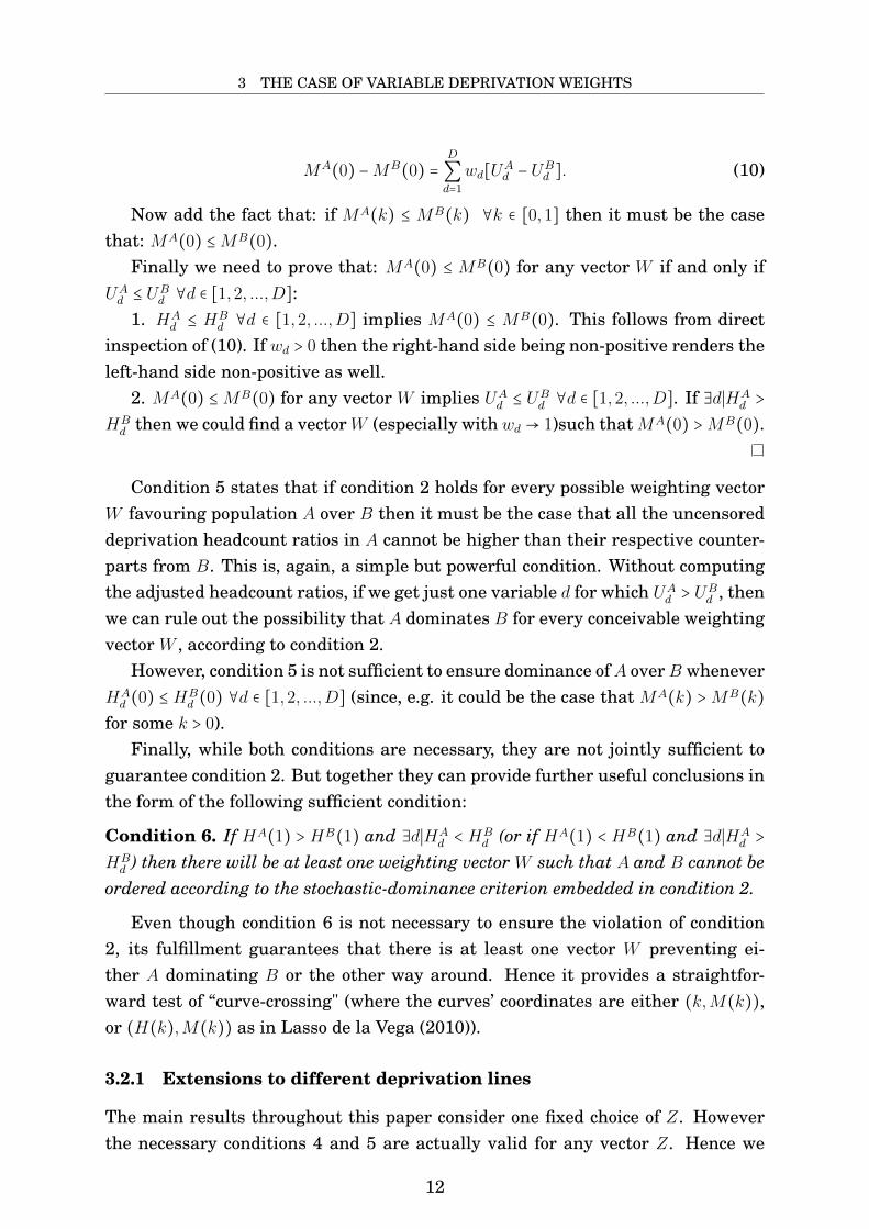
Now add the fact that: if MA(k) ≤ MB(k) ∀k ∈ [0,1] then it must be the casethat: MA(0) ≤MB(0).

Finally we need to prove that: MA(0) ≤ MB(0) for any vector W if and only ifUAd ≤ UB

d ∀d ∈ [1,2, ...,D]:1. HA

d ≤ HBd ∀d ∈ [1,2, ...,D] implies MA(0) ≤ MB(0). This follows from direct

inspection of (10). If wd > 0 then the right-hand side being non-positive renders theleft-hand side non-positive as well.

2. MA(0) ≤MB(0) for any vector W implies UAd ≤ UB

d ∀d ∈ [1,2, ...,D]. If ∃d∣HAd >

HBd then we could find a vectorW (especially with wd → 1)such thatMA(0) >MB(0).

Condition 5 states that if condition 2 holds for every possible weighting vectorW favouring population A over B then it must be the case that all the uncensoreddeprivation headcount ratios in A cannot be higher than their respective counter-parts from B. This is, again, a simple but powerful condition. Without computingthe adjusted headcount ratios, if we get just one variable d for which UA

d > UBd , then

we can rule out the possibility that A dominates B for every conceivable weightingvector W , according to condition 2.

However, condition 5 is not sufficient to ensure dominance ofA overB wheneverHAd (0) ≤ HB

d (0) ∀d ∈ [1,2, ...,D] (since, e.g. it could be the case that MA(k) >MB(k)

for some k > 0).Finally, while both conditions are necessary, they are not jointly sufficient to

guarantee condition 2. But together they can provide further useful conclusions inthe form of the following sufficient condition:

Condition 6. If HA(1) > HB(1) and ∃d∣HAd < HB

d (or if HA(1) < HB(1) and ∃d∣HAd >

HBd ) then there will be at least one weighting vector W such that A and B cannot be

ordered according to the stochastic-dominance criterion embedded in condition 2.

Even though condition 6 is not necessary to ensure the violation of condition2, its fulfillment guarantees that there is at least one vector W preventing ei-ther A dominating B or the other way around. Hence it provides a straightfor-ward test of “curve-crossing" (where the curves’ coordinates are either (k,M(k)),or (H(k),M(k)) as in Lasso de la Vega (2010)).

3.2.1 Extensions to different deprivation lines

The main results throughout this paper consider one fixed choice of Z. Howeverthe necessary conditions 4 and 5 are actually valid for any vector Z. Hence we

12

4 STATISTICAL INFERENCE

can consolidate all the results from the previous section in the following set ofnecessary conditions:

Condition 7. If MA(k) ≤ MB(k) ∀k ∈ [0, v2, ...,1] ∧ ∃k∣MA(k) < MB(k) for allpossible weighting vectors W and all possible deprivation-line vectors Z then: (1)HA(1) ≤HB(1) for all all deprivation-line vectors Z; and (2) UA

d ≤ UBd ∀d ∈ [1,2, ...,D]

for all possible deprivation-line vectors Z.

4 Statistical inference

4.1 Test of condition 2

In the empirical illustration, we first test condition 2 for a particular choice of W(equal weights). While different tests are possible, we implement a convenient onein which a null hypothesis of MA(k) ≤ MB(k) for every relevant value of k (i.e.values that the score cn can take given a set of weights and deprivation lines) isset against an alternative whereby ∃k∣MA(k) >MB(k). Basically if we do not rejectthe null we can state that either A dominates B or the two distributions perfectlyoverlap, which implies that poverty in A can never be above B for the given choiceof weights and deprivation lines, and for any poverty function considered in con-dition 2. Alternatively, rejecting in favour of the alternative means that "A doesnot dominate B", i.e. either A is dominated by B or the two curves of adjustedheadcount ratios cross (which in turn implies that the poverty comparison is sen-sitive to the choice of poverty functions and/or k, even for a given set of weightsand deprivation lines).

In practice, we can have a joint intersection null hypothesis: Ho ∶ MA(k) =

MB(k) ∀k ∈ [0, v2, ...,1] against a union alternative Ha ∶ ∃k∣MA(k) > MB(k). Forthat purpose, and considering that A and B are independently distributed, weconstruct the following statistics:

T (k) =MA(k) −MB(k)√

σ2MA(k)NA +

σ2MB (k)NB

, (11)

where:

σ2MA(k) ≡

1

NA

NA

∑n=1

[cn]2I(cn ≥ k) − [MA(k)]2 (12)

Then we test Ho ∶ T (k) = 0 against Ha ∶ T (k) > 0 for every relevant value ofk. Given the requirements of condition 2, we conclude that A does not dominatesB in terms of condition 2 if there is at least one k for which T (k) > Tα, where Tα

13

4 STATISTICAL INFERENCE

is the right-tail critical value for a one-tailed “z-test” corresponding to a level ofsignificance α. Since we test multiple comparisons, the actual size of the wholetest is not α. Under reasonable assumptions, it can be shown that it is β = ∑

li=1[l −

i + 1]αi(−1)i−1. We choose α = 0.01, so that β ≈ 0.05.


The testing procedure relies on the formula in (11) but now we have only onecomparison based on T (1). Plus we note that in the case of k = 1 the formula forthe variance simplifies to:

σ2MA(1) =H(1)[1 −H(1)] (13)

Then we test Ho ∶ T (1) = 0 against Ho ∶ T (1) > 0, using standard critical valuesfor a one-tailed “z-test”. If we reject the null then we conclude that A does notdominate B, irrespective of W .


The testing procedure is exactly the same as the one used for condition 2 but nowwe construct the following statistics:

Td =UAd −UB

d√

σ2

UAd

NA +σ2

UBd

NB

, (14)

where:

σ2UAd≡ UA

d [1 −UAd ] (15)

If we reject the null then we conclude that it is not true that A dominates B forevery conceivable weighting vector W .


The testing procedure is exactly the same as the one used for condition 2 but nowwe construct statistics for each sub-dimensional intersection headcount, similar tothose in (11) and (14). For example, in the case of Hi,j we have:

Ti,j =HAi,j −H

Bi,j

√σ2

HAi,j

NA +

σ2

HBi,j

NB

, (16)

where:

14

5 EMPIRICAL ILLUSTRATION: MULTIDIMENSIONAL POVERTY IN PERU

σ2HA

i,j≡HA

i,j[1 −HAi,j] (17)

If we reject the null then we conclude that it is not true that A dominates B forevery conceivable weighting vector W .

5 Empirical illustration: Multidimensional povertyin Peru

5.1 Background and data

As mentioned, Peru experienced a commodity boom between 2003 and 2007, whichtranslated into high GDP growth rates, from 4 % in 2003 to 8.9 % in 2007, and asteady decrease in monetary poverty headcounts, from 58.7 % in 2004 to 42.4 %in 2007. However, between 2008 and 2013, Peru’s economic performance was af-fected by the world economic situation: GDP growth fell from 9.8 % in 2008 to 0.9% in 2009, and then stabilized at around 7 % between 2010 and 2013. Notwith-standing this fluctuation, monetary poverty levels kept decreasing steadily, from37.3 to 27.8 %. How did the Peruvian population fare in terms of non-monetarymultidimensional poverty?

For this anonymous assessment of robust egalitarian poverty reduction withcounting measures, we use the Peruvian National Household Surveys (ENAHO) of2002 and 2013. Our multidimensional poverty measure relies on four dimensions,and on the household as the unit of analysis. Firstly, household education, com-prising two indicators: (1) school delay, which is equal to one if there is a householdmember in school age who is delayed by at least one year, and (2) incomplete adultprimary, which is equal to one if the household head or his/her partner has notcompleted primary education. The household is considered deprived in educationif any of these indicators takes the value of one.

The second dimension considers two indicators on infrastructure dwelling con-ditions: (i) overcrowding, which takes the value of one if the ratio of the number ofhousehold members to the number of rooms in the house is larger than three; and(ii) inadequate construction materials, which takes the value of one if the walls aremade of straw or other (almost certainly inferior) material, if the walls are madeof stone and mud or wood combined with soil floor, or if the house was constructedat an improvised location inadequate for human inhabitation. The household isdeprived in living conditions if any of the above indicators takes the value of one.

The third dimension is access to services. The household is deemed deprivedin this dimension if any of the following indicators takes the value of one: (i) lack

15


of electricity for lighting, (ii) lack of access to piped water, (iii) lack of access tosewerage or septic tank, and (iv) lack of access to a telephone landline. The fourthdimension is household vulnerability to dependency burdens. The household isdeprived or vulnerable if household members who are younger than 14 or olderthan 64 are three times or more as numerous as those members who are between14 and 64 years old (i.e. in working age).

We weigh each dimension equally. Therefore the household score can take onlyany of the following five values: (0,0.25,0.5,0.75,1).

5.2 Results

5.2.1 Point estimates

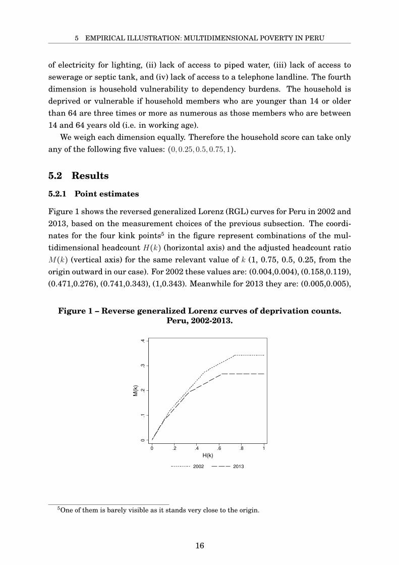
Figure 1 shows the reversed generalized Lorenz (RGL) curves for Peru in 2002 and2013, based on the measurement choices of the previous subsection. The coordi-nates for the four kink points5 in the figure represent combinations of the mul-tidimensional headcount H(k) (horizontal axis) and the adjusted headcount ratioM(k) (vertical axis) for the same relevant value of k (1, 0.75, 0.5, 0.25, from theorigin outward in our case). For 2002 these values are: (0.004,0.004), (0.158,0.119),(0.471,0.276), (0.741,0.343), (1,0.343). Meanwhile for 2013 they are: (0.005,0.005),

Figure 1 – Reverse generalized Lorenz curves of deprivation counts.Peru, 2002-2013.

0.1

.2.3

.4

M(k

)

0 .2 .4 .6 .8 1

H(k)

2002 2013

5One of them is barely visible as it stands very close to the origin.

16


(0.104,0.079), (0.333,0.194), (0.625,0.267), (1, 0.267). The curve for 2013 isnever above that of 2002, except for when k = 1. Hence condition 2 is not ful-filled. Based exclusively on the point estimates, we cannot conclude that, given aparticular choice of deprivation lines and dimensional weights, multidimensionalpoverty in Peru decreased between 2002 and 2013, along with a reduction in depri-vation inequality among the poor, for a broad family of inequality-sensitive povertyindices (at least those in (2)) and for any relevant choice of the poverty cut-off k.

Figure 2 shows the experiences of urban and rural areas between 2002 and2013. Again, in both cases, the 2013 curve is below that of 2002, except for areversal close to the origin, when k = 1. Hence, based only on the point estimates,we cannot confirm that both regions experienced poverty reduction accompaniedby lower inequality among the poor for any inequality-sensitive index and choiceof k.

Figure 3 shows the RGL curves for the five rainforest Peruvian departments(the dotted lines are for 2002, and the dashed lines for 2013). Except for the casesof San Martin and Ucayali, condition 2 is fulfilled, pointing to "pro-poorest" povertyreduction (dashed RGL lines representing 2013 appear always below dotted linesrepresenting 2002). By contrast, in San Martin and Ucayali, the RGL curve ishigher in 2013 for k = 1, meaning that the most severe forms of poverty (with k = 1)increased between 2002 and 2013.

Figure 2 – Reverse generalized Lorenz curves of deprivation counts.Urban and rural Peru, 2002-2013.

0.0

5.1

.15

.2.2

5

M(k

)

0 .2 .4 .6 .8 1

H(k)

Urban

0.1

.2.3

.4.5

M(k

)

0 .2 .4 .6 .8 1

H(k)

Rural

2002 2013

17


Figure 3 – Reverse generalized Lorenz curves of deprivation counts.Peruvian rainforest provinces, 2002-2013.

0.1

.2.3

.4.5

M(k

)

0 .2 .4 .6 .8 1

H(k)

Amazonas

0.1

.2.3

.4

M(k

)

0 .2 .4 .6 .8 1

H(k)

Madre de Dios

0.1

.2.3

.4.5

M(k

)

0 .2 .4 .6 .8 1

H(k)

Loreto0

.1.2

.3.4

M(k

)

0 .2 .4 .6 .8 1

H(k)

San Martin

0.1

.2.3

.4

M(k

)

0 .2 .4 .6 .8 1

H(k)

Ucayali

2002 2013

Figure 4 shows the RGL curves for the four southernmost Peruvian depart-ments, comprising both coastal and highland regions. In the case of Arequipa the

18


two curves cross once very close to the origin. Then the 2013 curve appears alwaysbelow the 2002 curve. This means that the assessment of inequality and povertyreduction depends on measurement choices. For example, with the intersection ap-proach (k = 1), poverty actually increased in Arequipa during the period, whereasfor less stringent identification approaches (k < 1) the conclusion depends on thechoice of both k and individual poverty functions. By contrast, Moquegua, enjoyingthe benefits of a thriving mining industry spread across a small population, sawa robust reduction of poverty accompanied by a decrease in inequality among thepoor. Puno’s case is similar to Arequipa’s: the curves cross once at the highest lev-els of k rendering the poverty assessment inconclusive. Likewise, the most severeforms of poverty (with k = 1) in Puno increased between 2002 and 2013. Finally,Tacna’s situation mimicks Puno’s and Arequipa’s: curve-crossing at the highestlevels of k. However, unlike Puno and Arequipa, Tacna’s curves are closer to theorigin in both years, reflecting lower (robust) poverty levels in both years. Tacnabenefits both from its mining industry and its active border with Chile.

Figure 5 shows the RGL curves for five south-central Peruvian departments,also comprising both coastal and highland regions. In the cases of landlockedCusco and mainly coastal Ica their respective pairs of curves cross at the high-est levels of k so that poverty reduction is not robust. Again, with an intersec-tion approach, both departments actually saw increases in the most severe formsof poverty. By contrast, the other three departments did experience fully robustpoverty reduction with lower deprivation inequality among the poor.

Figure 6 shows the RGL curves for five central Peruvian departments (includ-ing coastal and highland regions) and the coastal, city-sized, autonomous Callaoprovince. All cases show a robust poverty reduction accompanied by inequalityreduction, with the exceptions of the landlocked Junin and Huanuco. For the twolatter departments, there is, again, a curve crossing at the highest levels of k, justas in the previous situations of curve-crossing encountered so far.

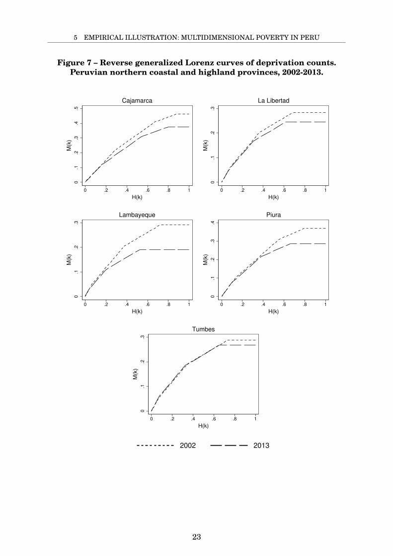
Figure 7 shows the RGL curves for the five northern Peruvian Departmentsalong the coast and the highlands. Except for Cajamarca, all departments featurecurve-crossing at the highest levels of k, just as in the previous cases of crossingabove. Hence the conclusion of poverty reduction with lower inequality between2002 and 2013 is not robust to all choices of k or functional forms. For instance,with an intersection approach, this extreme form of poverty actually increasedthroughout the region (except for Cajamarca).

19


Figure 4 – Reverse generalized Lorenz curves of deprivation counts.Peruvian southern coastal and highland provinces, 2002-2013.

0.0

5.1

.15

.2.2

5

M(k

)

0 .2 .4 .6 .8 1

H(k)

Arequipa

0.1

.2.3

M(k

)

0 .2 .4 .6 .8 1

H(k)

Moquegua

0.1

.2.3

.4

M(k

)

0 .2 .4 .6 .8 1

H(k)

Puno

0.0

5.1

.15

.2

M(k

)

0 .2 .4 .6 .8 1

H(k)

Tacna

2002 2013

20


Figure 5 – Reverse generalized Lorenz curves of deprivation counts.Peruvian south-central coastal and highland provinces, 2002-2013.

0.1

.2.3

.4

M(k

)

0 .2 .4 .6 .8 1

H(k)

Ayacucho

0.1

.2.3

.4

M(k

)

0 .2 .4 .6 .8 1

H(k)

Apurimac

0.1

.2.3

.4

M(k

)

0 .2 .4 .6 .8 1

H(k)

Cusco0

.1.2

.3.4

.5

M(k

)

0 .2 .4 .6 .8 1

H(k)

Huancavelica

0.0

5.1

.15

.2.2

5

M(k

)

0 .2 .4 .6 .8 1

H(k)

Ica

2002 2013

21


Figure 6 – Reverse generalized Lorenz curves of deprivation counts.Peruvian central coastal and highland provinces, 2002-2013.

0.1

.2.3

.4

M(k

)

0 .2 .4 .6 .8 1

H(k)

Ancash

0.0

5.1

.15

M(k

)

0 .2 .4 .6 .8 1

H(k)

Callao

0.1

.2.3

.4.5

M(k

)

0 .2 .4 .6 .8 1

H(k)

Huanuco

0.1

.2.3

.4

M(k

)

0 .2 .4 .6 .8 1

H(k)

Junin

0.0

5.1

.15

.2

M(k

)

0 .2 .4 .6 .8 1

H(k)

Lima

0.1

.2.3

.4

M(k

)

0 .2 .4 .6 .8 1

H(k)

Pasco

2002 2013

22


Figure 7 – Reverse generalized Lorenz curves of deprivation counts.Peruvian northern coastal and highland provinces, 2002-2013.

0.1

.2.3

.4.5

M(k

)

0 .2 .4 .6 .8 1

H(k)

Cajamarca

0.1

.2.3

M(k

)

0 .2 .4 .6 .8 1

H(k)

La Libertad

0.1

.2.3

M(k

)

0 .2 .4 .6 .8 1

H(k)

Lambayeque0

.1.2

.3.4

M(k

)

0 .2 .4 .6 .8 1

H(k)

Piura

0.1

.2.3

M(k

)

0 .2 .4 .6 .8 1

H(k)

Tumbes

2002 2013

23


5.2.2 Test results for condition 2

Table 1 shows the T (k) statistics for relevant values of k, as required for the testof condition 2, which we apply to the national, urban, and rural samples. In thethree cases we reject the null hypothesis, using the aforementioned 5% overallsignificance level, in favour of the alternative whereby poverty robustly decreasedin an egalitarian manner between 2002 and 2013.6

Table 1 – Ho ∶M2002(k) =M2013(k)∀k versus Ha ∶ ∃k∣M2002(k) >M2013(k)

k National Urban Rural0.25 31.862 24.784 25.7580.5 29.742 20.580 25.1580.75 16.519 11.881 11.5651 -0.763 -0.261 -0.954

Table 2 shows the T (k) statistics for the test of condition 2, involving the rain-forest provinces. With them we uphold the alternative hypothesis of robust egali-tarian poverty reduction, except in the case of Ucayali, for which we have evidenceof statistically significant curve-crossing.


k Amazonas Loreto Madre de Dios San Martin Ucayali0.25 7.454 5.987 5.549 7.103 2.1890.5 7.296 5.181 5.188 6.610 2.7190.75 3.788 4.609 4.435 3.711 0.7411 0.581 0.619 1.328 -0.613 -2.268

Table 3 shows the T (k) statistics for the test of condition 2, involving the south-ern provinces. We reject the null hypothesis in all cases, except for Arequipa. Weconclude robust egalitarian poverty reduction for Tacna and Moquegua. By con-trast, we find evidence of significant curve-crossing in the case of Puno.


k Puno Arequipa Tacna Moquegua0.25 3.391 2.002 2.901 8.0190.5 2.950 1.576 1.874 6.8440.75 -0.678 0.658 0.045 3.1371 -2.456 -1.000 -1.735 0.724

Table 4 shows the T (k) statistics for the test of condition 2, involving thesouthern-central provinces. For the whole region we reject the null hypothesis

6The signs of T (1) are actually in contradiction to the other sings, yet in none of the samplesT (1) is significantly different from zero.

24


in favour of the alternative of robust egalitarian poverty reduction between 2002and 2013.


k Cusco Ayacucho Apurimac Huancavelica Ica0.25 4.498 7.220 7.008 9.864 8.3070.5 5.096 6.885 7.098 10.742 6.4460.75 1.906 4.742 3.742 4.565 2.6831 -0.664 0.700 2.245 0.853 -1.865

Table 5 shows the T (k) statistics for the test of condition 2, involving the centralprovinces. Again, for the whole region we reject the null hypothesis in favour ofthe alternative of robust egalitarian poverty reduction between 2002 and 2013.


k Pasco Huanuco Callao Junin Lima Ancash0.25 5.728 9.340 2.181 7.202 7.907 10.4210.5 4.818 9.347 2.467 6.441 6.313 11.0740.75 3.503 5.682 2.243 4.635 4.098 6.3981 0.543 -0.881 0.422 -1.018 0.610 -0.068

Table 6 shows the T (k) statistics for the test of condition 2, involving the north-ern provinces. We reject the null hypothesis in favour of the alternative of robustegalitarian poverty reduction, except in the case of Tumbes.


k Tumbes La Libertad Cajamarca Piura Lambayeque0.25 1.587 3.586 7.901 7.838 9.8270.5 0.430 2.995 7.459 7.449 8.3280.75 -0.769 1.665 7.038 2.147 2.3841 -3.181 -1.000 1.718 -0.355 -0.555


Table 7 shows the T (1) statistics for the test of condition 4, which we apply tothe national, urban, and rural samples, as well as to the provinces. Results varywidely. With a 1% significance level (for simple one-tailed tests), we cannot rejectthe null hypothesis in the national, urban, and rural samples, nor in the case ofmost provinces. At that level of significance we only reject in favour of an alter-native hypothesis of higher intersection poverty (i.e. H(1)) in 2013 for the casesof Puno and Tumbes. By contrast, we never reject in favour of an alternative ofhigher intersection poverty in 2002.

25


Table 7 – Ha ∶H2002(1) =H2013(1) versus Ha ∶H2002(1) >H2013(1)

Department T(1) Department T(1)National -0.763 Junin -1.018Urban -0.261 La Libertad -1.000Rural -0.954 Lambayeque -0.555Amazonas 0.581 Lima 0.610Ancash -0.068 Loreto 0.619Apurimac 2.245 Madre de Dios 1.328Arequipa -1.000 Moquegua 0.724Ayacucho 0.700 Pasco 0.543Cajamarca 1.718 Piura -0.355Callao 0.422 Puno -2.456Cusco -0.664 San Martin -0.613Huancavelica 0.853 Tacna -1.735Huanuco -0.881 Tumbes -3.181Ica -1.865 Ucayali -2.268


Table 8 shows the Td statistics for each of the four dimensions involved in thetest of condition 5, which we apply to the national, urban, and rural samples.We find strong evidence against the fulfillment of condition 5 in favour of any ofthe two years. On one hand, clearly the uncensored deprivation headcounts foreducation, dwelling characteristics and access to services significantly decreasedbetween 2002 and 2013 (as is apparent from the size of their respective Td statis-tics). On the other hand, the uncensored deprivation headcount for dependencyburden significantly increased during the same period. In other words, we canconclude that the experience of egalitarian poverty reduction, documented earlierfor the national, urban, and rural samples, is not robust to any choice of weightingvectors. For example, given the particular test results in Table 8, we could selecta weighting vector heavily tilted toward the dependency burden dimension suchthat, together with other parameter and functional form choices, it would yield anincrease in poverty between 2002 and 2013, among the national, urban and ruralsamples. This would contrast with the robust egalitarian poverty reduction thatwe found above with a different set of weights.

Table 8 – Ho ∶ U2002d = U2013

d ∀d versus Ha ∶ ∃d∣U2002d > U2013

d

Ud National Urban RuralEducation 22.818 20.187 11.268Dwelling 20.701 12.661 16.193Services 37.414 24.917 42.225Burden -18.082 -11.423 -14.786

26

6 CONCLUDING REMARKS

6 Concluding remarks

This paper claimed that the second-order dominance condition of Lasso de la Vega(2010) and Chakravarty and Zoli (2009) is well-suited to ascertain the presence ofrobust egalitarian poverty reduction when poverty is measured using the countingapproach, and comparing two cross-sectional samples. When the condition holdswe can conclude that poverty decreased or increased consistently, in the sense thatthe result is robust to different choices of inequality-sensitive social poverty indicesand counting identification approaches. However these conditions only hold forspecific choices of deprivation lines and dimensional weights. With alternativeselections of the latter two parameter sets, the conditions would need to be testedagain.

Therefore in this paper we sought to refine the existing conditions by figur-ing out situations under which they would work for any choice of strictly positiveweights. We found the fundamental condition whose fulfillment is both necessaryand sufficient to ensure that second-order propositions work for any conceivableweighting vector with positive elements. However, since this condition may becumbersome to implement when the number of variables is large, we also derivedtwo useful conditions whose fulfillment is necessary, but insufficient, for robustsecond-order comparisons using any possible weighting vector. While these con-ditions are insufficient, they are fewer in number, and much easier to compute.When they are not met we can immediately rule out the robustness of second-order dominance in poverty reduction to any choice of weights.

Above and beyond the conditions derived in this paper, it is also possible toderive sets of necessary and sufficient conditions which guarantee robust egali-tarian poverty comparisons for a subset of weights, as well as for broader sets ofweights (e.g. admitting zero values). Likewise further useful necessary conditionsare derivable if we opt to restrict the set of admissible weighting vectors, or thedomain of k cut-offs, or both jointly. Some examples are available upon request.

Measuring poverty with indicators capturing dimensions of education, dwellinginfrastructure, service access and dependency burdens, the empirical illustrationshowed that 22 out of 25 Peruvian provinces experienced robust poverty reductionbetween 2002 and 2013, accompanied by lower deprivation inequality among thepoor. Similar results turned up for national, urban, and rural samples. Howeverthese findings relied on a fixed choice of deprivation lines and weights. When weprobed the national, urban, and rural cases further with our necessity conditions,we found that egalitarian poverty reduction was not robust to different weightingchoices.

Finally, the empirical illustration highlighted the importance of the intersec-

27

REFERENCES

tion headcounts, i.e. the proportions of people deprived in every dimension. Oftenthe differences between the intersection poverty headcounts of two samples werenot statistically significant. However, as it turned out in many comparisons, theadjusted headcount ratio of one sample would be consistently above another’s forevery poverty identification cut-off, except for the intersection approach (k = 1).Further studies based on a greater number of dimensions should help gauge thepervasiveness of this apparent relative difficulty in finding egalitarian povertycomparisons that remain robust when moving toward more stringent poverty iden-tification criteria.

References

Alkire, S. and J. Foster (2011). Counting and multidimensional poverty measure-ment. Journal of Public Economics 95(7-8), 476–87.

Alkire, S. and S. Seth (2014). Measuring and decomposing inequality among themultidimensionally poor using ordinal data: A counting approach. OPHI Work-ing Paper 68.

Ben Haj Kacem, R. (2013). Monetary versus non-monetary pro-poor growth: Evi-dence from rural ethiopia between 2004 and 2009. Economics: The Open-Access,Open-Assessment E-Journal, 7(26).

Berenger, V. and F. Bresson (2012). On the "pro-poorness" of growth in a multidi-mensional context. Review of Income and Wealth 58(3), 457–80.

Boccanfuso, D., J. Bosko Ki, and C. Menard (2009). Pro-poor growth measurementsin a multidimensional model: A comparative approach. GREDI Working Paper09-22.

Chakravarty, S. and C. D’Ambrosio (2006). The measurement of social exclusion.Review of Income and wealth 52(3), 377–98.

Chakravarty, S. and C. Zoli (2009). Social exclusion orderings. Working PapersSeries. Department of Economics. University of Verona.

Chakravarty, S. and C. Zoli (2012). Stochastic dominance relations for integervariables. Journal of Economic Theory 147, 1331–41.

Deutsch, J. and J. Silber (2011). On various ways of measuring pro-poor growth.Economics: The Open-Access, Open-Assessment E-Journal 5(13).

28

REFERENCES

Gallegos, J. and G. Yalonetzky (2014). Robust pro-poorest poverty reduction withcounting measures: the non-anonymous case. ECINEQ WP 2014 - 351.

Grimm, M. (2007). Removing the anonymity axiom in assessing pro-poor growth.Journal of Economic Inequality 5, 179–97.

Jenkins, S. and P. Lambert (1997). Three ‘i’s of poverty curves, with an analysis ofuk poverty trends. Oxford Economic Papers 49, 317–27.

Lasso de la Vega, C. (2010). Counting poverty orderings and deprivation curves.In J. Bishop (Ed.), Research on Economic Inequality, Volume 18, Chapter 7, pp.153–72. Emerald.

Silber, J. and G. Yalonetzky (2013). Poverty and Social Exclusion. New methods ofanalysis, Chapter 2, pp. 9–37. Routledge Advances in Social Economics. Rout-ledge.

29

Melbourne Institute Working Paper No. 22/2015 · 2016-11-07 · Melbourne Institute Working Paper...

Documents

Transcript of Melbourne Institute Working Paper No. 22/2015 · 2016-11-07 · Melbourne Institute Working Paper...