
MEEKATHARRA VIRTUAL SOLAR FARM WITH CENTRALISED SOLAR …
84
MURDOCH UNIVERSITY SCHOOL OF ENGINEERING AND INFORMATION TECHNOLOGY ENG470 ENGINEERING HONOURS THESIS 2016 MEEKATHARRA VIRTUAL SOLAR FARM WITH CENTRALISED SOLAR SMOOTHING BATTERY A report submitted to the School of Engineering and Information Technology, Murdoch University in partial fulfilment of the requirements for the degree of Bachelor of Engineering Honours [BE(Hons)] Electrical Power, Renewable Energy PIERCE LLEWELLYN TRINKL INDUSTRY SUPERVISOR: KELLI FRIAR ACADEMIC SUPERVISORS: DR. MARTINA CALAIS, CRAIG CARTER
Transcript of MEEKATHARRA VIRTUAL SOLAR FARM WITH CENTRALISED SOLAR …

M U R D O C H U N I V E R S I T Y
S C H O O L O F E N G I N E E R I N G A N D I N F O R M A T I O N T E C H N O L O G Y
E N G 4 7 0 E N G I N E E R I N G H O N O U R S T H E S I S
2 0 1 6
MEEKATHARRA VIRTUAL SOLAR FARM WITH
CENTRALISED SOLAR SMOOTHING BATTERY
A report submitted to the School of Engineering and Information Technology,
Murdoch University in partial fulfilment of the requirements for the degree of
Bachelor of Engineering Honours [BE(Hons)]
Electrical Power, Renewable Energy
PIERCE LLEWELLYN TRINKL
INDUSTRY SUPERVISOR: KELLI FRIAR
ACADEMIC SUPERVISORS: DR. MARTINA CALAIS, CRAIG CARTER

ii | Page Declaration
This page has intentionally been left blank

Declaration iii | Page
Declaration
I, Pierce Llewellyn Trinkl, certify that this work contains no material which has been
accepted for the award of any other degree or diploma in my name, in any university or
other tertiary institution and, to the best of my knowledge and belief, contains no material
previously published or written by another person, except where due reference has been
made in the text.
Word Count: 14,536
Signed: …………………………
Name: …………………………
Date: …………………………

iv | Page Abstract
Abstract
As increasing amounts of renewable energy systems are being integrated into traditional
power systems; a number of issues relating to the level of renewable energy penetration are
arising. Horizon Power, an operator of islanded microgrids in Western Australia, is
particularly susceptible to these problems as small microgrids can be destabilised by relatively
low amounts of renewable energy generation compared with larger interconnected systems.
This problem was brought to the forefront when a consortium of customers on Horizon
Power’s Meekatharra microgrid applied to install solar generation that would collectively
make up one third of Meekatharra’s maximum load.
This project is a feasibility study to determine the financial impact that connecting such a
large amount of renewable energy generation to the network will have on both the
customers and Horizon Power. It takes into consideration not only the impact of the solar
generation being installed but also the accompanying solar smoothing battery required to
allow such high renewable energy penetration. Furthermore, the possibility of a solar trading
platform, to allow customers on the network to trade their excess energy, was explored and a
financial model developed to assess the additional impact this would have on Horizon
Power.
HOMER Energy was used to model the expected energy flows of each individual customer
using real hourly load profiles supplied by Horizon Power. The requirements of the solar
smoothing battery, and an accompanying cost estimate, were developed in conjunction with
Horizon Power engineers using DIgSILENT’s PowerFactory. Financial modelling was
completed in Excel based on these energy flows and battery pricing estimates. Finally, the
likely value extracted from Horizon Power by a trading platform was estimated in Excel,
again using the HOMER energy flows as a basis.

Abstract v | Page
The outcomes of this study provided Horizon Power with a complete set of results to
consider, when deciding whether to invest in the project. The key finding was currently the
centralised solar smoothing battery is economically infeasible, leading to the decision not to
invest in this project at this time and instead to wait until battery prices have declined. Once
prices have reached the amount shown in the sensitivity analysis to make the project
economically feasible, it will be reconsidered and the models developed through this project
updated and re-simulated.

vi | Page Acknowledgements
Acknowledgements
Firstly, I would like to express my gratitude to my academic supervisor, Dr. Martina Calais,
not only for assisting and supporting me through my thesis but also for her commitment and
enthusiasm to teaching in the years leading up to this point. Thank you for helping me to
become the engineer I am today. I would also like to thank Craig Carter for his assistance
and feedback during the writing of my thesis, I appreciate your time.
To my industry supervisor Kelli Friar, thank you for allowing me to complete this project for
Horizon Power and your supervision and expertise offered throughout. The industry
experience I have gained from this project will be invaluable in starting my career as an
engineer.
Last but not least; thank you to all of the hard working and diligent staff at Murdoch
University who have taught or helped me throughout my degree.

Contents vii | Page
Contents
Declaration ................................................................................................................. iii
Abstract ....................................................................................................................... iv
Acknowledgements .................................................................................................... vi
Contents ..................................................................................................................... vii
Figures ......................................................................................................................... x
Acronyms ................................................................................................................... xii
Units xii
1.0 Introduction ....................................................................................................... 1
1.1 Horizon Power ................................................................................................................................... 1
1.2 Background ......................................................................................................................................... 3
1.3 Aims and Objectives .......................................................................................................................... 4
1.4 Project Tasks ....................................................................................................................................... 5
1.4.1 HOMER Energy Modelling ........................................................................................................ 5
1.4.2 Financial Modelling ....................................................................................................................... 5
1.4.3 Solar Smoothing Charge ............................................................................................................... 6
1.4.4 Battery Requirements .................................................................................................................... 7
1.4.5 Solar Energy Trading Platform ................................................................................................... 7
1.5 Thesis Outline ..................................................................................................................................... 8
2.0 Homer Modelling ............................................................................................. 9
2.1 Customer Load Data ......................................................................................................................... 9
2.2 Customer Deemed Load Profiles and Previous Years Consumption ..................................... 11
2.3 Scrubbing Load Data and Scaling Deemed Load Profiles ........................................................ 11
2.4 Extrapolating Data and Comparing Deemed Load Profile to Actual Load Profile .............. 12
2.5 Other required Information and Inputs for HOMER Models ................................................ 15
2.5.1 Number of PV modules in each array ...................................................................................... 15
2.5.2 Type of PV modules ................................................................................................................... 16
2.5.3 Other likely de-rating factors ..................................................................................................... 16

viii | Page Contents
2.5.4 Orientation and Pitch of Solar Modules .................................................................................. 17
2.5.5 Type of Inverters ......................................................................................................................... 17
2.5.6 Climate Data ................................................................................................................................. 18
2.6 Development of the HOMER Models......................................................................................... 19
2.7 HOMER Results .............................................................................................................................. 20
3.0 Financial Modelling ........................................................................................ 22
3.1 Customer Financial Model.............................................................................................................. 22
3.1.1 Data Input ..................................................................................................................................... 22
3.1.2 Calculations ................................................................................................................................... 26
3.1.3 Outcomes ...................................................................................................................................... 27
3.1.4 Sensitivity Analysis for Customer Finances ............................................................................ 30
3.2 Horizon Power Financial Model ................................................................................................... 34
3.2.1 Input Data ..................................................................................................................................... 34
3.2.2 Calculations ................................................................................................................................... 35
3.2.3 Outputs ......................................................................................................................................... 36
3.2.4 Sensitivity Analysis ...................................................................................................................... 37
3.3 Solar Smoothing Charge Financial Model .................................................................................... 38
3.3.1 Data Input ..................................................................................................................................... 39
3.3.2 Calculations ................................................................................................................................... 40
3.3.3 Outputs ......................................................................................................................................... 40
3.3.4 Sensitivity Analysis ...................................................................................................................... 41
4.0 Solar Smoothing Battery Requirements ......................................................... 43
4.1 Preliminary Design ........................................................................................................................... 43
4.2 Modelling ........................................................................................................................................... 45
5.0 Solar Energy Trading Platform ...................................................................... 48
5.1 Scenario One – Consortium Only ................................................................................................. 49
5.1.1 Consortium Only Model ............................................................................................................ 49
5.2 Scenario Two – All Customers ...................................................................................................... 50
5.2.1 All Customers Model .................................................................................................................. 50

Contents ix | Page
6.0 Conclusion ...................................................................................................... 52
6.1 Customer Summary ......................................................................................................................... 52
6.2 Horizon Power Summary ............................................................................................................... 53
6.3 Solar Trading Platform Summary .................................................................................................. 53
6.4 Future Work ...................................................................................................................................... 54
7.0 References ....................................................................................................... 55
8.0 Appendices ...................................................................................................... 57
8.1 Appendix A ....................................................................................................................................... 57
8.2 Appendix B ....................................................................................................................................... 59
8.3 Appendix C ....................................................................................................................................... 60
8.4 Appendix D ....................................................................................................................................... 65
8.5 Appendix E ....................................................................................................................................... 67
8.6 Appendix F........................................................................................................................................ 69
8.7 Appendix G ....................................................................................................................................... 71
8.8 Appendix H ....................................................................................................................................... 72

x | Page Figures
Figures
Figure 1: Horizon Power Supply Area [2] ........................................................................................ 2
Figure 2: Real Load Profile VS Deemed Load Profile ................................................................. 13
Figure 3: Closer View of Customer Nine Load Profiles .............................................................. 13
Figure 4: Customer Eight Mirrored AMI Load Profile ................................................................ 14
Figure 5: HOMER Solar Data ......................................................................................................... 18
Figure 6: HOMER Main Screen ...................................................................................................... 20
Figure 7: Customer Nine Payback Graph ...................................................................................... 29
Figure 8: Ramp Down ....................................................................................................................... 44
Figure 9: Voltage and Frequency Change during Cloud Event .................................................. 47
Figure 10: Customer One Payback Graph ..................................................................................... 60
Figure 11: Customer Two Payback Graph ..................................................................................... 60
Figure 12: Customer Three Payback Graph .................................................................................. 60
Figure 13: Customer Four Payback Graph .................................................................................... 61
Figure 14: Customer Five Payback Graph ..................................................................................... 61
Figure 15: Customer Six Payback Graph ....................................................................................... 61
Figure 16: Customer Seven Payback Graph .................................................................................. 62
Figure 17: Customer Eight Payback Graph ................................................................................... 62
Figure 18: Customer Nine Payback Graph .................................................................................... 62
Figure 19: Customer Ten Payback Graph ...................................................................................... 63
Figure 20: Customer Eleven Payback Graph ................................................................................ 63
Figure 21: Customer Twelve Payback Graph ................................................................................ 63
Figure 22: Customer Thirteen Payback Graph .............................................................................. 64

Figures xi | Page
Tables
Table 1: Meter Numbers and National Meter Identifiers .............................................. 10
Table 2: Customer Nine HOMER Model Outputs ...................................................... 20
Table 3: Financial Overview .................................................................................... 26
Table 4: Simple Payback Customer Nine ................................................................... 28
Table 5: Simple Payback Reached (Customer Nine) .................................................... 29
Table 6: NPV, IRR and Refined Simple Payback of Customer Nine .............................. 29
Table 7: Cost of System Sensitivity Analysis (Customer Nine) ....................................... 31
Table 8: Customer Bought Solar Smoothing Sensitivity Analysis (Customer Nine) ........... 32
Table 9: Solar Smoothing Charge Sensitivity Analysis (Customer Nine) .......................... 33
Table 10: Horizon Power Finance Model Input Overview ........................................... 35
Table 11: Horizon Power Finances ........................................................................... 36
Table 12: NPV Sensitivity Analysis ........................................................................... 37
Table 13: Net Cash Flow Sensitivity Analysis ............................................................. 38
Table 14: Input Overview ....................................................................................... 39
Table 15: Solar Smoothing Charge ............................................................................ 40
Table 16: Solar Smoothing Charge Sensitivity Analysis ................................................ 41
Table 17: Value Extracted by Consortium Members Only ............................................ 50
Table 18: Value Extracted by all Customers in Meekatharra .......................................... 51
Table 19: HOMER Modelling Outputs for all Customers ............................................ 57
Table 20: All Customers NPV, IRR and Simple Payback Period .................................... 59
Table 21: Cost of System Sensitivity Analysis Results for all Customers .......................... 65
Table 22: Customer Bought Solar Smoothing Sensitivity Analysis Results for all Customers
........................................................................................................................... 67
Table 23: Solar Smoothing Charge Sensitivity Analysis Results for all Customers ............. 69
Table 24: Horizon Power Yearly Net Cash Flow......................................................... 71

xii | Page Acronyms
Acronyms
Horizon Power HP
Western Australia WA
Photovoltaic PV
South West Interconnected System SWIS
Global Horizontal Irradiance GHI
Net Present Value NPV
Net Present Cost NPC
Renewable Energy Buyback Scheme REBS
Intellectual Property IP
Units
Kilowatt: measure of the rate of energy transfer kW
Kilowatt Hour: measure of energy kWh
Kilovolts: measure of electrical potential kV
Equations
1: Average Power……………………………………………………………………….....9
2: Scaling of Deemed Profile……………………………………………………………...12
3: Battery Energy Requirements…………………………………………………………..43

Introduction 1 | Page
1.0 Introduction
This project was completed for Horizon Power (HP) as an industry thesis by Pierce Trinkl,
as the final assessment towards a Bachelor of Engineering Honours. It was completed in the
second semester of 2016 over a 16 week period in which Pierce was employed full time by
HP to solve a problem they were facing.
As ever increasing numbers of people are wishing to reap the benefits of generating their
own electricity via solar photovoltaic (PV) systems, the utilities to which the houses of these
people are connected are facing issues that the power industry has not previously
encountered. This project was concerned with one of these newly arisen problems; the issue
of grid instability caused by high levels of PV penetration within a network.
This document begins by outlining to the reader who HP is and the exact issue that they
were facing. It then describes in detail, step by step, how the problem was solved; aiming to
give the reader enough detail to replicate the procedure.
1.1 Horizon Power
HP is the regional and remote electricity utility of Western Australia (WA), established in
2006 during reforms to WA’s electricity sector. It operates state wide, apart from the south
west region where electricity is supplied through the south west interconnected system
(SWIS). It services a total area of 2.3 million square kilometres, supplying 41 towns, 34 of
which are stand-alone microgrid systems in regional towns and remote communities [1].
Within these towns HP is responsible for the entire electrical process from generation or
procurement to distribution and retail. Customers include residential, industrial and
commercial and resource developments.

2 | Page Introduction
Figure 1: Horizon Power Supply Area [2]
Although the company is state government owned it remains commercially focused, running
a number of initiatives to reduce costs and stay competitive in the currently rapidly evolving
energy sector. With many of the towns being so remote, HP is in an interesting situation
where operating costs of conventional energy supply methods such as diesel generators are
extremely high. So high in fact that in many cases, new technologies that are still too costly
to implemented in larger networks may actually be financially viable. In recent years this has
led to much higher renewable energy penetration, especially PV, within their networks;
which in turn causes issues to arise that the larger networks may not yet have to deal with.
HP is now in the unique position where due to the drive to be competitive, high operating
costs and small network sizes, they can trial new technologies ahead of other utilities to
become one of the leaders in microgrid operation.

Introduction 3 | Page
1.2 Background
This project was taken on by HP when they were approached by a consortium of eight
business owners from Meekatharra. Meekatharra is a small town containing 487 private
dwellings with a population of 1377, as of the 2011 census [3]. It is located approximately
700km north-east of Perth in the mid-west region of WA with a hot and dry semi-arid
climate [4]. Lots of sunshine and low precipitation makes it well suited for solar PV.
Some of the businesses already have 5kW of solar PV installed on their rooftops, however;
they would like to have much more [5]. Due to high solar penetration, HP has made it
mandatory for any connections over 5kW of solar to be “generation managed” to maintain
grid stability [6]. This means that the output of the solar system may not ramp up or down at
a greater rate than HP stipulates in its generation management technical requirements [7].
In the case of solar this becomes an issue when broken cloud cover causes the PV output to
fluctuate wildly as clouds intermittently block the sun. Limiting the upwards ramp to HP’s
stipulated limit is easily managed by only allowing the inverter to ramp up power output at
that rate. However, limiting ramp down is not so easily achieved. When the solar modules
are covered by a cloud and their output drops almost instantly the inverter cannot ramp
down slower as there is no longer any power available; the inverter has to be receiving the
power from somewhere. A solution to this is to install a battery system that supplies the
required power while the output is ramped down [7].
The consortium decided that the cost of a battery system of the size required for their arrays
would make upgrading to a larger array uneconomical and thus approached HP. In their
initial application they also floated the idea of a trading platform that would be run by HP
but would allow them to trade their excess solar energy with each other [5]. HP agreed to
undertake this project as both the utility owned solar smoothing service and the solar trading
4 | Page Introduction
platform are pieces of infrastructure that they believe will soon become more prevalent and
early development and adaptation will put them in a strong position for the future.
1.3 Aims and Objectives
The main aim of this project is to assess and model the impact of 13 photovoltaic arrays,
totalling 428kW of capacity, owned by eight business customers, connecting to HP’s
Meekatharra power distribution network. A further aim is to develop the technical
requirements of one large centralised solar smoothing battery system that will be installed to
maintain grid stability during a cloud event. Finally the preliminary development of a solar
trading platform with which the customers can trade their excess solar energy is also
incorporated in the project.
The study includes:
- Modelling of the network impact of the 13 arrays using the real load data from the
premises at which they are installed;
- Financial modelling of the impact to customers and HP;
- The development of a solar smoothing charge structure for customers to pay for
the service;
- The technical requirements for the solar smoothing battery system to be compliant
with HP’s generation management standards;
- The foundations of a solar energy trading platform.
The 13 arrays are modelled using HOMER Energy, a versatile program that is capable of in-
depth modelling and simulation of microgrids. The grid can be created with as many or few
elements as required, even down to a single house and allows for all common renewable
Introduction 5 | Page
energy sources. The operation of the grid, or in this case house, is then simulated by
calculating the energy flows on an hourly basis.
The financial models are developed in Microsoft Excel and the battery’s technical
requirements are based on a network study performed using DIgSILENT’s PowerFactory.
PowerFactory is a power system analysis program for applications in generation,
transmission and distribution. It is used to develop detailed models of networks, which are
then used to analyse how the network will function or react in different scenarios.
1.4 Project Tasks
1.4.1 HOMER Energy Modelling
An individual model for each of the 13 installations was created using HOMER Energy with
the main outcomes being the energy generated, energy self-consumed and energy exported
to the grid annually for each customer. The customer load profile was required to model
generation against usage, giving the energy consumed and exported. For accuracy, the real
customer load data was used, which was acquired through HP’s new Advanced Metering
Infrastructure (AMI). Also required for accurate results were the size, number and type of
PV modules and inverters, NASA solar radiation and temperature data and pitch and
orientation of the array. This information was gathered from a number of sources including
HP’s data base, Google maps and the NASA website for surface meteorology and solar data.
1.4.2 Financial Modelling
A financial model on the impact of installing rooftop PV for each of the eight customers
including, NPV, IRR and simple payback period was developed using Microsoft Excel.

6 | Page Introduction
These financial models required the annual energy self-consumed/exported by each
customer, derived from the previously completed HOMER Energy models, along with the
cost of electricity and the feed in tariff. The financial models also required a number of
financial statistics such as the cost of capital, inflation, hurdle rate, expected tariff growth,
the corporate tax rate and a production decline factor to account for age related degradation
of the solar arrays. These financial statistics were sourced from HP’s finance department.
One overall financial model incorporating the summation of all of the customer’s energy
transfers was created to observe the impact of installing such a large amount of solar PV on
HP’s network. In addition to financial information required for the customer models, HP’s
model required the cost of generation. The term of the project for both the customers and
HP, for financial modelling purposes, was 15 years as designated by HP’s finance
department.
Only a rough estimate of the cost of the arrays and the solar smoothing battery was required
as sensitivities around the cost of the system, cost of solar smoothing battery, feed in tariff,
cost of generation (HP) and cost of solar smoothing service were performed to gain a deeper
understanding of the effect this project will have on both the customers and HP.
1.4.3 Solar Smoothing Charge
HP has never before provided a solar smoothing service to its customers; previously it has
been the customer’s responsibility to install smoothing technology that meets HP’s
generation management technical requirements. This being the first time such a service has
been offered required the generation and development of ideas around possible charge
structures for customers to pay HP for this new service. At this stage in the project, the
financial models for both the customers and HP were completed and were used to observe
the impact different pay structures and prices would have. Different price structures were

Introduction 7 | Page
developed in conjunction with HP’s experts and the financial impacts on both the customers
and HP modelled for review by the appropriate HP staff.
1.4.4 Battery Requirements
The technical requirements of the solar smoothing battery were developed so that it meets
HP’s generation management technical requirements, which are stipulated as the minimum
requirements for customers that would like to connect more than 5kW [7] of solar
generation to HP’s network. The network was then modelled, by Horizon Power engineers,
using DIgSILENT’s PowerFactory including the arrays and the chosen solar smoothing
battery. Using the outcomes of this system study it was then determined if the battery system
developed according to HP’s customer standards is sufficient to maintain a stable network
even in the worst case scenario that is probable to occur. If the battery system was found
insufficient or there was too greater risk to the network, the battery requirements were
modified and the system re-simulated until an acceptable outcome was achieved.
1.4.5 Solar Energy Trading Platform
The eight business customers of the consortium would not only like to connect a large
amount of solar generation to HP’s network but also use the network to trade excess solar
energy between themselves. If all customers were to do this HP would be maintaining a
network for free whilst the trading customers reap all the benefits; clearly an unsustainable
situation. However, HP recognises that the future of energy generation is distributed and
adapting to this sooner rather than trying to resist will be advantageous long term.
HP had no preconceptions about what form such a trading platform would take. It could be
a physical system, with extra metering and infrastructure being installed, or a purely digital

8 | Page Introduction
system of accounting; using their newly connected AMI. Ideas for this platform were
developed as a part of this project through discussion with HP experts and through research
into any similar platforms or systems that may already be functioning or in development.
The aim of this section was to gain an understanding of how much value such a trading
platform may withdraw from HP’s network and thus how much remuneration HP can
reasonably expect for maintaining the network. This culminated in a financial model of a
possible energy trading platform, based on the energy flows of the 13 customers in the
consortium as modelled via HOMER Energy.
1.5 Thesis Outline
This thesis consists of six chapters and electronic appendices. Chapter one introduces the
problem, provides background on HP and the project, and outlines the specific tasks
performed. Chapter two steps through the HOMER modelling process giving details about
the inputs required, paying extra attention to the customer load profiles, and the outputs
obtained. Three describes the financial modelling for the customers, HP, the solar
smoothing charge and sensitivity analyses for all three. Four shows the design process for
the requirements of the solar smoothing battery. Chapter five presents the solar trading
platform, the developed model and its financial impact on HP. Chapter six summarises the
conclusions and suggests further work and finally the appendices provide supporting
documentation and the full sets of results.

Homer Modelling 9 | Page
2.0 Homer Modelling
2.1 Customer Load Data
The load profile required for this project is the average power used by a customer during
each hour of the year. The AMI that HP has been installing across its networks stores
customer’s energy usage in 15minute intervals. This can be converted into hourly average
power by summing up the four 15minute intervals that make up an hour. As energy is
measured in kWh and power is measured in kW, finding the average power for the hour is
achieved by dividing the energy used in that hour by 1h. All of the load data manipulation
was done using Microsoft Excel.
Equation 2.1 below is an example of how this is calculated.
1: Average Power
To obtain this load data a list of meter numbers was to be given to a HP engineer who
would then access the database and withdraw the hourly load data for each of the meters.
Unfortunately the meter numbers that were listed in the original customer application
document [5], from which all the necessary information was to be obtained, were the old
meters. The meters had since been switched out to the new AMI. These new meters took
readings every 15 minutes and stored the value rather than only a cumulative value that was
read every 3 months. These new meters made it possible to model the systems on an hourly
basis using HOMER Energy.
To overcome this issue a list of all the new meter numbers and their addresses was retrieved
to be cross-referenced with the addresses listed in the customer application document. This

10 | Page Homer Modelling
did not work as some of the addresses were listed in unit numbers rather than street
numbers; giving no matches.
Fortunately HP uses a National Meter identifier (NMI) number, which is a geolocation
identifier, as well as the meter numbers. This NMI was also listed in the original application
allowing a comparison with a list of all 431 Meekatharra customers, retrieved from HP’s
database, to find the meter numbers for the new meters in those locations. As the meters
were only swapped out, it was safe to say that the new meters would be in the same location
as the old meters.
Table 1 below, shows a censored version of the customers with their meter numbers and
NMI.
Table 1: Meter Numbers and National Meter Identifiers
At this stage at least six months’ worth of real load data had been acquired for all of the
customers besides one, which only had the meter swapped one month ago.

Homer Modelling 11 | Page
2.2 Customer Deemed Load Profiles and Previous Years Consumption
Obtaining the deemed load profiles was completed without complication as they were stilled
listed with the old meter numbers, however; one customer did not have a deemed load
profile. This customer was the same customer that also only had their meter swapped one
month ago. It was decided that one month of data is insufficient for accurate modelling.
A solution was to search for real load data of any similar customers who may have had their
meter changed earlier and scale that load so that the total yearly consumption was the same.
The Meekatharra customer was a mining camp full of dongas and the town of Port Hedland
had their meters changed first so they had a sufficient amount of data available. Five mining
camp load profiles from Port Hedland were retrieved in the hopes of finding a close match,
with data available over a longer time period.
The previous year’s total consumption, which is required to scale the deemed load profile to
the customers actual usage, was also obtained without complication. In the previous year the
customers still had the old meters so the meter numbers were given to HP’s metering
services department, which retrieved and sent back the data.
2.3 Scrubbing Load Data and Scaling Deemed Load Profiles
The real load profiles had gaps in them, usually indicating a power outage but also possibly a
communication error. These were few enough that filling them with the average value of that
respective profile was an acceptable approximation. The same method was used to complete
the Port Hedland mining camp load profiles.
The deemed load profiles were scaled so that the total yearly consumption matched that of
the previous year. To do this a scaling fraction was calculated from the previous year’s

12 | Page Homer Modelling
consumption and the total yearly consumption of the deemed profile. Each hour within the
year was then multiplied by that fraction, giving a profile of the same shape but scaled to the
real total consumption. Equation 2.2 below demonstrates how the scaling fraction was
calculated and applied to each hour.
2.4 Extrapolating Data and Comparing Deemed Load Profile to Actual Load
Profile
The aim of this sub-task was to have the most accurate load profile available for each of the
customers for an entire year. This would then be the final form that would be used in
HOMER to model that customer’s array and their effect on HP’s network.
A process of elimination was used to decide what this most accurate profile would be for
each customer.
First the available real customer data was compared to the deemed load profile for that
respective customer. This comparison was done visually by graphing the same month of
both profiles over each other and inspecting.
Figure 2 below, shows customer nine who’s real load profile was a close match with the
deemed profile.
2: Scaling of Deemed Profile

Homer Modelling 13 | Page
Figure 2: Real Load Profile (AMI) vs Deemed Load Profile
A shorter period of the same customer was then graphed for a more detailed comparison;
this is shown in Figure 3 below.
Figure 3: Closer View of Customer Nine Load Profiles
If the two profiles were a very close match, they were further compared by calculating the
day/night energy use ratio for the months of available real data and the same months of the
deemed profile. Day use was considered to be 7am until 5pm to bring it in line with solar

14 | Page Homer Modelling
generation as this was a rough way of comparing how similar the use during solar generation
and without solar generation was. This was the most important factor as the main sought
after outcomes of the modelling were the energy self-consumed and energy exported to the
grid. All profiles that visually looked similar also had almost identical day/night energy use
ratios. It was decided that for these customers the deemed load is sufficiently accurate to be
used in the modelling.
For the remaining customers that had more than six months of available data, the data began
within the first two weeks of January. This coincided with the middle of summer. It was
decided that beginning from as close to mid-January as possible until six months later would
make up the first six months of the load profile. Flipping over or mirroring the first six
months then created the second six months of the load profile. As the available data spanned
from the middle of summer to the middle of winter, seasonal variability would be accounted
for by using this method.
Figure 4 below, shows the yearlong profile that was created for customer eight by flipping
six months of available real AMI load data. Notice the seasonal variability of lower use in
winter and higher use in summer is captured in this profile.
Figure 4: Customer Eight Mirrored AMI Load Profile

Homer Modelling 15 | Page
After completing the above steps there was one remaining customer who did not have a
yearlong load profile that was sufficiently accurate to be used for modelling. This customer
was the donga mining camp, which did not have a deemed load profile and only one month
of available real data. To develop a load profile for this customer, five load profiles spanning
an entire year of similar customers from Port Hedland had previously been retrieved and
scrubbed. The one month of available real data for the customer was compared to the same
month of the Port Hedland mining camps using the same method as used above for the
deemed profiles. Fortunately one of the camps in Port Hedland was very similar to the camp
in Meekatharra. This profile was chosen to be used for modelling.
2.5 Other required Information and Inputs for HOMER Models
Once the load profiles were finalised all of the other information and inputs required for the
HOMER models were acquired. This information was gathered from a variety of sources, all
of which are listed with the information and the reason it is required in the sub-sections
below.
2.5.1 Number of PV modules in each array
The number of PV modules in each array along with the rated output, sourced from the
application [5], was used to calculate the total output of the array in kWp. This is used in
HOMER as part of the equation to calculate the output power of the array for each hour of
the year [8].

16 | Page Homer Modelling
2.5.2 Type of PV modules
The type of PV modules was also contained within the original customer application form
[5]. This was used to find the specifications sheet for the panels as a number of
specifications are used by HOMER. These include the rated output, temperature coefficient
and nominal operating temperature.
The nominal operating temperature, the temperature coefficient and the ambient
temperature are used to calculate the temperature de-rating factor. PV cells become less
efficient at higher temperatures, producing less power. This must be accounted for in the
model for accurate results, giving rise to a de-rating factor. HOMER takes this one step
further and recalculates the temperature de-rating factor for each hour of the year [8]. The
panels are therefore, more efficient in the morning when they are still cool and less efficient
during the peak heat of the day.
2.5.3 Other likely de-rating factors
A number of other de-rating factors are likely to reduce the output of the solar modules
throughout their operational lifetime. HOMER combines all of the de-rating factors besides
temperature such as soiling, manufacturing tolerances, wiring losses, system availability and
shading into one scaling factor that is applied uniformly [8].
The modules used in this project have a manufacturing tolerance of +5W/-0W and it is
assumed that the arrays are not shaded. This leads to a mild combined de-rating factor of 0.9
for wiring losses, soiling and system availability from commonly used values for these de-
rating factors [9].

Homer Modelling 17 | Page
2.5.4 Orientation and Pitch of Solar Modules
The orientation and pitch of solar arrays can also have a large impact on how much energy
they produce. The optimal facing is of course directly at the sun; however, this would require
a tracking system that is not included in this project. For stationary solar arrays in the
southern hemisphere, the optimal orientation is due north with a pitch angle, in degrees,
equal to the latitude angle of their location [10]. HOMER, given the location and global
horizontal irradiance calculates the solar irradiance that an array of given orientation and
pitch would receive in each hour and uses this to calculated the power output [8].
The orientation of each of the solar arrays was obtained by using Google maps to look at the
roof spaces where the arrays will be located. Using the compass feature it was possible to
find the heading of the roof space in degrees west of south, which is the form that HOMER
requires [8].
Unfortunately it was not possible to measure the pitch of the roofs using Google earth as the
images were of insufficient clarity for such a precise purpose. Due to this, the HOMER
default value was used for all of the customer’s arrays.
2.5.5 Type of Inverters
The type of inverter was also available from the original customer application form [5]. This
was required so that the specifications sheet could be found, which contained the inverter
size and its efficiency. HOMER requires the inverter size and efficiency to calculate how
much power is lost through the inverter and the maximum possible power transfer [8]. Solar
arrays are oversized to make up for the de-rating factors mentioned in section 2.5.3 above.
This means that on a day with perfect conditions the solar array’s output may be higher than

18 | Page Homer Modelling
anticipated, possibly even higher than the inverter’s rating. In this scenario the inverter will
limit the power to its rating even though the panels could produce more.
2.5.6 Climate Data
The climate data, especially solar, is one of the most important pieces of information that
HOMER requires as this forms the basis for power and therefore energy production [8]. The
solar data comes in two parts; the monthly average Global Horizontal Irradiance (GHI),
which is the total beam and diffuse irradiance on a horizontal surface, and the monthly
clearness index, which is a measure of the clearness of the atmosphere. A clearness index
value closer to zero indicates a cloudy month and a value closer to 1 indicates a clear month
[8]. HOMER uses both of these values to calculate the likely irradiance to impact on a solar
module for each hour of the year, randomly adding cloudy days of low irradiance in
accordance to the clearness index [8]. The HOMER screen showing the GHI and clearness
index is shown below in Figure 5.
Figure 5: HOMER Solar Data

Homer Modelling 19 | Page
The temperature data is not as critical as the GHI as it is only used to de-rate the modules as
described in section 2.5.2. Both the GHI data and temperature data were sourced from
NASA’s surface meteorology and solar energy website [11] as HOMER has an inbuilt option
to retrieve this data. Otherwise HOMER does allow for manual input of data where it is
necessary [8].
2.6 Development of the HOMER Models
Using all of the information gathered and the load profiles, it was now possible to develop
the individual HOMER models for each of the 13 customers. Creating the models within
HOMER is achieved by adding the required components and their parameters plus the
climate data. All of this information and its importance has been explained throughout
chapter two of this report.
HOMER usually also requires some economic parameters for cost optimisation and system
control parameters for battery and diesel operation. However, in this case HOMER is only
being used for the annual energy flows of the system so these parameters were not necessary.
Below in Figure 6 is the main screen of HOMER. Along the top is a list of all of the
components that can be added, to the left is a diagram showing the complete system of
customer eight and in the central area is a map with any comments.

20 | Page Homer Modelling
Figure 6: HOMER Main Screen
2.7 HOMER Results
The sought after results of annual energy generated, energy self-consumed and energy
exported to the grid, by the PV array, are displayed within HOMER’s results section in a
manner that makes them easy to extract. These results, from each of the separate customer
models, were tabulated in one excel spread sheet for later use in the financial models. Table 2
below shows the results for customer nine as an example.
Table 2: Customer Nine HOMER Model Outputs
Customer Nine
HOMER Output Amount in kWh
Annual energy generated 21609
Annual energy exported 0
Annual energy consumed internally 21609

Homer Modelling 21 | Page
% of self-consumption 100.00%
% fed into grid 0.00%
The complete results are attached in appendix A, the models themselves could not be
provided as they were created at HP and are therefore HP Intellectual Property (IP).
22 | Page Financial Modelling
3.0 Financial Modelling
3.1 Customer Financial Model
Before making 13 versions of the financial spreadsheet, one for each customer, a base
version was created and perfected to be passed to HP for review. This spreadsheet was
broken up into 3 sections; data input, calculations and output. Once this had been reviewed,
one was made for each customer with their specific information and a sensitivity analysis
completed.
3.1.1 Data Input
This portion of the spreadsheet is where all of the information required for calculating the
impact that the solar array will have on the customer’s finances is entered. This includes the
financial parameters as well as the energy data acquired from the HOMER Energy
modelling.
3.2.1.1 Cost of Funding
The cost of funding is the percentage interest that is incurred for borrowing the funds
necessary to install the solar PV system. HP decided that for this model 100% of the funds
would be borrowed at 5.5% interest [12]. The interest rate was selected as it is an average
mortgage interest rate that can be expected to be incurred in the likely case that the customer
pays for the system by using funds from their home loan.

Financial Modelling 23 | Page
3.1.1.2 Hurdle Rate
HP required that the hurdle rate be 5.5% [12] so that at a minimum the system is making the
customer enough money to pay for the cost of capital. The hurdle rate is also used when
calculating the Net Present Value (NPV) and Net Present Cost (NPC) to discount future
cash flow. Higher hurdle rates shift the focus to the earlier years as the later years are so
heavily discounted that their impact on the NPV or NPC becomes negligible.
3.1.1.3 Expected Tariff and Renewable Energy Buyback Scheme (REBS) Growth
The expected tariff and REBS growth rate is the rate at which HP’s financial department
expects these tariffs to increase. HP currently expects an increase of 4.5% per annum for the
next 4 years and 2.5% thereafter [12]. The tariff increases are stipulated by the Western
Australian state government and therefor HP has no control over the amounts. However,
HP does have control over the REBS rates, which means that they do not have to increase
uniformly with other tariff rates. HP stated that for this model it can be assumed that all
tariff rates will grow at the same rate.
3.1.1.4 Company Tax Rate
The company tax rate in Australia is a constant rate of 30% [13] so this was used in the
model. This is amount of money has to be taken away from any profit made in the model or
conversely if a loss is made the company will save this much of the loss on tax as the total
taxable income will be less.

24 | Page Financial Modelling
3.1.1.5 Tariff Rates and REBS
Collectively within the 13 consortium members there were four different tariff rates being
charged. These were N2 57.706 cents per kWh, L4 33.9633 cents per kWh, L2 and K2 both
at 30.3104 cents per kWh [14]. The tariffs are used in the model to calculate how much
money the customers will save by using a number of kWh of their own solar generation
rather than buying energy from HP.
The REBS rate is also required for the model to calculate how much money the customers
will earn by selling their excess energy to HP. The exact value cannot be given as HP and the
consortium will agree on a non-standard rate, taking into account that HP would be
installing the centralised battery system. The standard rate varies from town to town and can
be found on the HP website; Meekatharra is currently 26.41 cents per kWh [15].
3.1.1.6 Annual Energy Self Consumed
This input is acquired from the results of the HOMER energy modelling and is accordingly
different for each customer. It is the amount of kWh of energy that the customer no longer
needs to buy from HP as it is meeting the load directly with the generation from the solar
system. It is used in the model, along with the tariff rate, to calculate the amount of money
the customer will save by installing the PV system.
3.1.1.7 Annual Energy Exported to the Grid
This input is also acquired from the results of the HOMER energy modelling and is
accordingly different for each customer. It is the amount of excess kWh that the system will
produce at times when there is only a low load with higher solar generation. The customer

Financial Modelling 25 | Page
can sell this excess to HP through the REBS. The amount of money that they will make is
calculated in the model with this parameter and the REBS rate.
3.1.1.8 Annual Decline in Production
This parameter is used in the model to account for the reduced production of the solar
modules as they age and degrade over the life of the project. The reduction of energy
generated by the solar modules and therefore the system was evenly distributed over the
internal consumption and grid exports even though in reality the exports would be more
heavily reduced. A value of 0.9% was used to err on the conservative side as the datasheet
for the solar modules used, states a reduction of not more than 0.6% per annum [16].
3.1.1.9 Price of Photovoltaics per kW
The price per kW of PV for simplicity represents the total system cost per kW of rated
output including the solar modules, inverter, roof racks, installation and any other balance of
system costs. The price used for the model is $2500 as this is the value HP uses for remote
PV installations such as Meekatharra [12]. This parameter is used by the model to calculate
the capital costs of each of the differently sized systems.
3.1.1.10 System Size in kW
Each of the customers has a differently sized system according to the available north facing
roof on their specific building. The model uses the size along with the price per kWh to
calculate the capital cost of each system.

26 | Page Financial Modelling
3.1.1.11 Input Overview
Table 3 below is an overview of all of the financial parameters and assumptions
Table 3: Financial Overview
Financial Overview
Parameter Amount Assumption
Cost of Funding 5.5% 100% borrowed
Hurdle Rate 5.5% NA
Expected Tariff Growth 4.5% for 4 years, 2.5% after
Company Tax Rate 30%
Tariff Rates
N2 57.706 cents per kWh L4 33.9633 L2, K2 30.3104
Annual Energy Self Consumed Varies for each customer
Consider each customer individually
Annual Energy Exported to the Grid Varies for each customer
Consider each customer individually
Annual Decline in Production 0.9% Slightly higher than module specifications
Price of PV per kW $2500 High as it is for a remote town
System size in kW Varies for each customer Consider each customer individually
3.1.2 Calculations
The project lifetime and therefore also the modelling period is 15 years, with each year from
one to 15 simply a repetition of the same calculations. With a slight exception for year zero
which is different as it is considered the year in which the solar system was installed so there
is no production. It exists only to show the initial capital costs of the project. As an example,
the calculations in year zero and one will be outlined below.
Year zero first calculates the capital cost from the size of the system and the cost per kW of
PV. This is then used to determine the net cash flow which is simply an outgoing of the cost
of the PV system. This cost of the system is also used to calculate the depreciation of the
value of the asset for tax purposes by dividing the cost of the system by 15 years so that the

Financial Modelling 27 | Page
asset depreciates by the same amount each year until it is worth $0 at the end of the life of
the project. The total cost of the system and the interest rate are also used at this stage to
calculate the cost of capital as a yearly interest only repayment.
The subsequent years are more complicated as there are more inputs to take account of. The
tariff from the last year has the expected tariff growth rate added whilst the energy
production values from the HOMER modelling are reduced by the annual decline in
production. The energy self-consumed, which is left after the production decline factor has
been taken into account, is multiplied by the customer’s tariff to give the self-consumption
benefit. The feed in tariff is multiplied by the exported energy, which is left after the
production decline has been taken into account, giving the export benefit to the customer.
The net value of the depreciation of the solar panels, the cost of capital, the self-
consumption benefit and export benefit is calculated so that the tax benefit or tax payable of
the customer can be calculated. The tax is calculated by multiplying the net effect of the
above four parameters by the business tax amount.
The net cash flow of that year is then calculated by summing the self-consumption benefit,
the export benefit, the cost of capital and the tax of customers. This process is then repeated
for each year to give the net financial impact that the system has on the business for the 15
year life of the project.
3.1.3 Outcomes
Once the 15 years of net cash flows has been calculated the useful outputs that this process
has been trying to achieve can be calculated. To do this Microsoft Excel has some handy
inbuilt functions that were used.

28 | Page Financial Modelling
The NPV was calculated using the NPV function within Excel. This function requires the
total cost of the system which was calculated in year zero along with the net cash flow for
each of the 15 years and the hurdle rate as a benchmark to measure the value against. IRR
was calculated similarly with the IRR function within Excel. This function simply uses the
net cash flows of each year with the first one being negative the total capital cost of the
system.
The third output that was required was the simple payback period, unfortunately excel does
not have a function for this but it can be done manually. To do this, new rows had to be
created. The new rows were the cumulative cash outflows of each year, which was the initial
capital cost in year zero plus the outflows in each year for the following 15 years. The
cumulative benefit, which was the sum of the self-consumption benefit and the export
benefit. And the cumulative net cash flow, which was the cumulative cash outflows plus the
cumulative benefit. The year in which the cumulative net cash flow changed from a negative
to a positive is the year in which simple payback has been reached. To clarify this the first
three years from customer nine have been included in Table 4 below.
Table 4: Simple Payback Customer Nine
Customer Nine
Year 1 2 3
Cumulative Benefit (Self-consumption benefit + export benefit) $7,600 $15,471 $23,620
Cumulative Cash Outflow ( Initial capital + yearly cash outflows) -$33,295 -$34,089 -$34,884
Cumulative Net Cash flow (Cumulative cash outflow + cumulative benefit) -$25,694 -$18,618 -$11,264
Payback Identifier False False False
The simple payback was further refined through linear interpolation by finding the ratio
between how much the cumulative net cash flow had increased that year and how much was
still required to get to $0. This ratio then became the fraction of the year that was required to

Financial Modelling 29 | Page
pay back the PV system. Table 5 below, is once again customer nine showing the year when
simple payback was reached.
Table 5: Simple Payback Reached (Customer Nine)
Customer Nine
Year 3 4 5
Cumulative Benefit $23,620 $32,057 $40,634
Cumulative Cash Outflow -$34,884 -$35,678 -$36,473
Cumulative Net Cash flow -$11,264 -$3,622 $4,151
Payback Identifier False False True
Below in Table 6 the NPV, IRR and simple payback period of customer nine are shown. The
results for all customers are shown in appendix B.
Table 6: NPV, IRR and Refined Simple Payback of Customer Nine
Customer Nine
NPV $47,447
IRR 22%
Simple Payback 4.47 years
Using the cumulative values it was then also possible to graph the payback period for a visual
representation of the value of the system to the customer. Figure 7 below shows the graph
that was created for customer nine. The graphs for all customers are attached in appendix C.
Figure 7: Customer Nine Payback Graph

30 | Page Financial Modelling
These results showed that for customer nine installing the PV array without any form of
solar smoothing would be a very profitable investment. Not all of the customers had such
favourable financial outcomes. Depending on their load profiles and the size of their array,
the financial outcomes indicated that for some customers it would not be financially
beneficial to install the solar and in fact it would be better for them to continue buying all of
their power from the grid. The customers for whom the investment was favourable have a
load profile that allows them to use a high percentage of what their PV generates, thus
benefiting more. The customers for whom the investment is unfavourable have a load
profile that forces them to sell most of the energy that their PV produces, thus losing out on
the higher savings. The full set of results is provided in appendices A and B. The models
themselves are not available as they are HP IP.
3.1.4 Sensitivity Analysis for Customer Finances
A sensitivity analysis was performed for each of the customers once HP had reviewed the
financial spreadsheet and signed off on it. The sensitivity analysis was performed to gain a
deeper understanding of the customer’s financial situation by analysing how changes in
prices would affect their outcomes. The parameters changed within the models were the
price of PV per kW, the feed in tariff, the price for customer bought solar smoothing and a
possible solar smoothing charge. The solar smoothing charge was developed based on the
solar smoothing battery requirements, which is explained in chapter 4. For simplicity all of
the financial modelling is grouped together; however, it took place at different stages
throughout the project as the necessary information became available.

Financial Modelling 31 | Page
3.1.4.1 Price of PV per kW
It was decided that the initial price of $2500 per kW of installed PV capacity is most likely
the highest price that the customers would pay even including the inverter, installation and
balance of system costs. Because of this decision, the sensitivity analysis started at $2500 and
decreased in increments of $500. The outcome of this sensitivity analysis is shown for
customer nine in Table 7 below. The full set of results for all customers is presented in
appendix D.
Table 7: Cost of System Sensitivity Analysis (Customer Nine)
Price of Solar ($/kW) $ 2,500 $2,000 $1,500 $1,000
NPV $47,447 $55,542 $63,637 $71,732
IRR 22.20% 28.74% 39.10% 59.08%
Payback (Years) 4.47 3.55 2.65 1.76
These results showed, as expected, for all of the customers, that decreasing the price of the
system greatly improved their financial situation.
3.1.4.2 Feed in Tariff
The exact value of the feed in tariff cannot be shown as this will be an agreement between
HP and the consortium of customers. A number of different feed in tariffs were modelled to
see the impact this would have on the customers. The results of this are not shown in this
report as they would be useless without the values used for the feed in tariff. HP’s current
public REBS rate is 26.41 cents per kWh of energy imported to the grid.
The results from the feed in tariff sensitivity analysis were varied as the impact was
dependent on the amount of energy that was exported to the grid. Because of this the
financial outcomes of customers that did not export much energy only changed very slightly

32 | Page Financial Modelling
whereas customers that exported most of their energy were greatly impacted by this
sensitivity.
3.1.4.3 Customer Bought Solar Smoothing Batteries
To better understand why the customers could not afford to install solar smoothing with
their PV systems the price of a solar smoothing system was added to their models. Prices
from $500 to $2000 per kW of installed PV were modelled in increments of $500. Table 8
below shows the results obtained for customer nine. The full set of results for all customers
can be found in appendix E.
Table 8: Customer Bought Solar Smoothing Sensitivity Analysis (Customer Nine)
Customer Bought Smoothing ($/kW) $0 $500 $1,000 $1,500 $2,000
NPV $47,447 $39,352 $31,257 $23,162 $15,067
IRR 22.20% 17.58% 14.07% 11.27% 8.95%
Payback (Years) 4.47 5.41 6.37 7.36 8.37
These results show, as expected, that the customer’s financial situation becomes worse as the
price of solar smoothing increases. Customer nine, used as an example here, varies from a
sound business investment to one that would most likely be rejected from a business
perspective. In some cases customers who were already struggling to be financially viable
without the solar smoothing, no longer had a simple payback within the 15 years of the
project lifetime.

Financial Modelling 33 | Page
3.1.4.4 Solar Smoothing Charge Sensitivity
The solar smoothing charge was developed as an alternative to customers buying their own
solar smoothing batteries. It was developed in the hopes that a large centralised system
would be less costly than 13 separate small batteries. Once the charge had been developed it
was added to the customer’s financial models and a sensitivity analysis completed. Table 9
below shows the solar smoothing charge sensitivity analysis for customer nine as an example.
The results of all customers are shown in appendix F.
Table 9: Solar Smoothing Charge Sensitivity Analysis (Customer Nine)
Solar Smoothing Service ($/kW.Month) $0.00 $62.80 $118.22 $229.06 $339.91
NPV $47,447 $37,360 $28,459 $10,656 -$7,146
IRR 22.20% 19.11% 16.25% 10% 2.00%
Payback (Years) 4.47 5.05 5.70 7.79 12.81
The price of the solar smoothing charge that had to be passed on to customers so that HP
would not be making a loss on the battery system was the highest amount that can be seen in
table 8 above. It was decided that rather than doing a plus and minus sensitivity analysis a
better understanding would be gained by decreasing the charge to find the level at which the
customers could afford it. This would give HP an indication of how much the price of the
battery system would have to decrease before it become economically viable.
The results above show that even customer nine who had very positive financial results
could not afford to pay the full solar smoothing charge. At roughly a third of the price
customer nine’s simple payback period and IRR came back into the bounds where a business
would consider the investment. This also meant that HP would have to be able to install the
centralised solar smoothing battery at one third of the original estimated price. All of the
sensitivity results besides the feed in tariff are included in appendix D, E and F. The models
themselves again could not be included as they are HP IP.
34 | Page Financial Modelling
3.2 Horizon Power Financial Model
Once each of the individual customer finances had been completed, one spreadsheet that
modelled the combined impact that the entire consortium would have on HP’s finances was
developed. This model was created by editing the same spreadsheet that was previously
developed for the customers as many sections were the same. The only extra piece of
information that was required was the cost of generation. This was used to calculate HP’s
savings due to no longer having to generate the energy that the solar arrays would be
supplying. The model was again broken up into the three sections; data input, calculations
and outputs.
3.2.1 Input Data
All of the inputs from the customer modelling were kept with slight changes to the annual
energy self-consumed and annual energy exported. As the HP financial model must take into
account all of the 13 separate customers the total energy self-consumed and exported by the
entire consortium had to be taken into account. This was done by creating separate inputs
for each of the four different tariffs that the customers within the consortium were charged.
For each tariff the total energy self-consumed for all the customers on that particular tariff
was calculated and these four amounts become the new inputs. The total energy exported by
all of the customers was also calculated but did not need to be grouped into tariffs as all
customers would be receiving the same feed in tariff. Each of the tariffs is given in section
3.1.1.5 above in the customer financial section. HP’s cost of generation was also added as an
input to the spreadsheet and set at 20c per kWh.

Financial Modelling 35 | Page
3.2.1.1 Input Overview
Table 10 below, is an overview of all of the financial parameters and assumptions
Table 10: Horizon Power Finance Model Input Overview
Input Overview
Parameter Amount Assumption
Hurdle Rate 5.5% NA
Expected Tariff Growth 4.5% for 4 years, 2.5% after
Company Tax Rate 30%
Tariff Rates
N2 57.706 cents per kWh L4 33.9633 L2, K2 30.3104
Annual Energy Self Consumed Varies for each customer
Consider total of all customers
Annual Energy Exported to the Grid Varies for each customer
Consider total of all customers
Annual Decline in Production 0.9% Slightly higher than module specifications
Price of PV per kW $2500 High as it is for a remote town
System size in kW Varies for each customer Consider total of all customers
Cost of Generation 20c per kWh
3.2.2 Calculations
The calculation section in this model was also very similar to the calculations in the customer
model. The project lifetime was the same at 15 years with each year a repetition of the year
before. However, year zero was not required as HP was not investing any money besides the
battery, which was used in a separate model to develop the solar charge and so was not
required in this model.
To calculate the cash flow in each year the tariff from the last year has the expected tariff
growth rate added, whilst the summed energy production values from the HOMER
modelling are reduced by the annual decline in production. The total energy self-consumed,

36 | Page Financial Modelling
remaining after the production decline factor, for each of the separate tariffs is multiplied by
the corresponding tariff cost to give the self-consumption loss to HP. The feed in tariff is
multiplied by the total exported energy of all of the customers in the consortium that is left
after the production decline has been taken into account, giving the export loss to HP. And
the total self-consumption and total export energy of all 13 customers is multiplied by the
generation cost to give the benefit to HP of not having to generate that energy.
The net impact of the above cash flows can then be used to calculate the tax impact on HP.
As the net value of the cash flows is a negative value, HP will no longer have to pay taxes on
that income giving a slight relief from the loss.
The net cash flow of that year is finally calculated by summing the self-consumption loss, the
export loss, the cost of generation benefit and the tax benefit. This process is then repeated
for each year to give the net financial impact that the system has on the business over the 15
year life of the project.
3.2.3 Outputs
The outputs that HP was interested in were the NPV of the project over the whole 15 years
and the yearly loss, which allowing these customers to install PV systems would cause. The
NPV was calculated using Excels NPV function the same as in section 3.1.3 above, whilst
the yearly loss was already displayed as the net cash flow for each year. The yearly loss
increased with each year as the tariffs rates increased, this can be seen in appendix G. Table
11 below shows the NPV and the loss incurred in the first 3 years.
Table 11: Horizon Power Finances
Horizon Power Finances
Year 1 Year 2 Year 3
Net Present Value -$334,352 Net Cash Flow -$33,353 -$34,536 -$35,759

Financial Modelling 37 | Page
3.2.4 Sensitivity Analysis
In this case the sensitivity analysis was performed to gain a deeper understanding of how two
of the parameters would affect HP’s finances. First the cost of generation was analysed as it
has a large effect on HP and it is a highly variable parameter that depends on the price of oil.
Secondly the feed in tariff was analysed by using the same feed in tariff prices that were used
in the customer’s sensitivity analysis. This was done so that HP would have a complete
picture on how the feed in tariff affects both its own finances and the customer finances at
corresponding prices. Having this complete picture would allow HP to negotiate a fair price
with the customers.
Both the cost of generation and the feed in tariff were varied by +/- 10%, 25% and 50%, as
per HP’s finance department [12], simultaneously to create a table with all possible
combinations. Excel has a handy function called “What-If Analysis, Data Table” that
simplifies this process immensely. This was then repeated for both the NPV and net cash
flow and some conditional formatting layered over the top to colour code the improved and
worsened scenarios so that the table can be understood at a glance. The NPV and net cash
flow are shown in Table 12 and 13, respectively, below.
Table 12: NPV Sensitivity Analysis
Sensitivity of NPV Feed in Tariff
-$344,352 50% 25% 10% 0% -10% -25% -50%
Cost of Generation
50% $5,300 $96,570 $151,333 $187,841 $224,349 $279,112 $370,383
25% -$260,797 -$169,526 -$114,764 -$78,256 -$41,747 $13,015 $104,286
10% -$420,455 -$329,184 -$274,422 -$237,914 -$201,405 -$146,643 -$55,372
0% -$526,894 -$435,623 -$380,861 -$344,352 -$307,844 -$253,082 -$161,811
-10% -$633,333 -$542,062 -$487,299 -$450,791 -$414,283 -$359,520 -$268,250
-25% -$792,991 -$701,720 -$646,957 -$610,449 -$573,941 -$519,178 -$427,908
-50% -$1,059,087 -$967,817 -$913,054 -$876,546 -$840,038 -$785,275 -$694,004
In the centre of the table in the white cell is the base scenario where both the cost of
generation and feed in tariff have not been altered. The rows vary from feed in tariff +50%

38 | Page Financial Modelling
to -50% and the columns vary from cost of generation +50% to -50% giving all possible
combinations. Red cells indicate that the NPV is worse than the base case, yellow indicates it
is better than the base case but still negative and green indicates that the NPV is above 0$.
Table 10 shows that for the NPV to become positive the cost of generation has to increase
by 25% to 50% and feed in tariff has to decrease by 25% to 50% at the same time.
Table 13: Net Cash Flow Sensitivity Analysis
Sensitivity of Net Cash Flow Feed in Tariff
-33352 50% 25% 10% 0% -10% -25% -50%
Cost of Generation
50% $513 $9,353 $14,657 $18,193 $21,729 $27,033 $35,873
25% -$25,259 -$16,419 -$11,115 -$7,579 -$4,043 $1,261 $10,100
10% -$40,723 -$31,883 -$26,579 -$23,043 -$19,507 -$14,203 -$5,363
0% -$51,032 -$42,192 -$36,888 -$33,352 -$29,816 -$24,512 -$15,672
-10% -$61,341 -$52,501 -$47,197 -$43,661 -$40,125 -$34,821 -$25,981
-25% -$76,804 -$67,964 -$62,660 -$59,124 -$55,588 -$50,284 -$41,444
-50% -$102,576 -$93,736 -$88,433 -$84,897 -$81,361 -$76,057 -$67,217
Table 13 is structured and can be read the same as table 10; however, this one shows the net
cash flow rather than the NPV. It displays very similar results in the fact that for the net cash
flow to become positive the cost of generation must be 25% to 50% higher and the feed in
tariff 25% to 50% lower, simultaneously. This is expected as the NPV is based on the net
cash flow of the project.
3.3 Solar Smoothing Charge Financial Model
The solar smoothing charge was modelled after the battery requirements had been
developed; however, to keep all of the financial sections together within this document it has
been placed before.
Once the battery requirements had been passed on to HP an initial price estimate of
$1,500,000 was supplied from which the solar smoothing charge was developed. This was

Financial Modelling 39 | Page
once again completed using Microsoft Excel by creating a spreadsheet that calculated the
NPV of the battery over a 15 year lifetime. HP decided that they do not need to make a
profit on this system; however, the solar smoothing charge must be enough to ensure that
they do not make a loss. Making a loss was defined as having a negative NPV over the 15
year lifetime.
This spreadsheet was structure similarly to the previous customer finances with a data input,
calculations and output section and a year zero.
3.3.1 Data Input
The data required for this model is the tariff growth rate, the corporate tax rate, the hurdle
rate, the total size of the solar arrays installed by the consortium and the annual price of the
solar smoothing charge per kW of installed PV. The price of the annual solar smoothing
charge per kW of installed PV was optimised to make the NPV $0. This was also a pricing
structure that ensured that all customers could be charged fairly across a multitude of array
sizes.
3.3.1.1 Input Overview
Table 14 below, is an overview of all of the financial parameters and assumptions
Table 14: Input Overview
Input Overview
Parameter Amount Assumption
Hurdle Rate 5.5% NA
Expected Tariff Growth 4.5% for 4 years, 2.5% after
Company Tax Rate 30%
Tariff Rates
N2 57.706 cents per kWh L4 33.9633 L2, K2 30.3104

40 | Page Financial Modelling
Annual Solar Smoothing Price per kW of installed PV Unknown
This was the variable this model was estimating
System size in kW Varies for each customer Consider total of all customers
3.3.2 Calculations
In year zero the cost of the battery is invested as a loss to HP and that amount used to
calculate the yearly depreciation of the asset so that it reaches $0 at the end of the project
life. In each of the following years, first the annual solar smoothing charge is increased by
the tariff growth rate. This is then multiplied by the 428kW of total capacity that the
consortium wishes to install, giving the benefit to HP. The depreciation of the battery and
the benefit to HP are summed and the outcome, along with the corporate tax rate, used to
calculate the effect that this system will have on HP’s taxes. Finally the outgoing and
incoming cash flows are summed, which are the solar smoothing charge benefit and the tax,
to give the net cash flow for that year. This process is repeated for all 15 years.
3.3.3 Outputs
The output that this model gave was the NPV, which was obtained by using Excel’s NPV
function with the hurdle rate set at 6.27%. However, the output that was required from this
model was annual solar smoothing charge per kW of installed PV capacity. To obtain this
the model was run in reverse using the “Goal Seek” function within Excel. “Goal Seek” was
used to seek an NPV of $0 by varying the solar smoothing charge input. The result of this
process is shown below in Table 15 below.
Table 15: Solar Smoothing Charge
Solar Smoothing Financial Modelling
Cost of Battery $1,500,000
Annual Solar Smoothing Charge $399.91

Financial Modelling 41 | Page
(per kW of PV)
The results of this process were fed back into the customer financial model as can be seen in
section 3.1.4.4. This showed that the solar smoothing charge was unaffordable for the
customers and that HP would have to install the battery at a lower price or be willing to
make a loss on this project. Once this was discovered a sensitivity analysis was completed on
the solar smoothing charge and the results again fed into the customer finances as shown in
3.1.4.4.
3.3.4 Sensitivity Analysis
The solar smoothing charge at this price was completely unaffordable for most customers, in
some cases it eroded any benefit the customer would receive by installing the solar array. At
this stage HP reassessed their previous cost estimate and concluded that the given price
would most likely be a maximum price. With this information the sensitivity analysis was
only performed for lower battery prices by changing the cost of the battery in year zero of
the model and then performing a new goal seek. Table 16 below shows the results of the
sensitivity analysis, these values are the values that were then used in section 3.1.4.4 above.
Table 16: Solar Smoothing Charge Sensitivity Analysis
Solar Smoothing Financial Modelling
Cost of Battery $1,500,000 $1,000,000 $500,000 $250,000
Annual Solar Smoothing Charge (per kW of PV) $399.91 $229.06 $118.22 $62.80
On their own the results above are hard to understand as they are prices that seem arbitrary.
For a deeper understanding and some reference as to the effect that these different prices

42 | Page Financial Modelling
have on the customers refer back to section 3.1.4.4. The price at which this charge became
affordable to customers was $118.22 or $500,000 for the battery system.

Solar Smoothing Battery Requirements 43 | Page
4.0 Solar Smoothing Battery Requirements
A solar smoothing system is required for grid stability as explained in section 1.2. The
requirements of the solar smoothing battery were developed so that the system would be
able to meet HP’s stipulated ramp rates, which are given within HP’s generation
management technical requirements document. The document states that any solar array
larger than 5kW may not ramp up at a greater rate than 0% to 100% in six minutes. This is
easily achieved by limiting the ramp up rate through the inverter. It also states a maximum
ramp down rate of 100% to 0% in 12 minutes [7]. This is achievable only through the
installation of a battery system to supply power during ramp down. To ensure that the
battery will meet the ramp down rate, two stages of development were completed. These
were the preliminary design, followed by modelling of the network including the array and
the solar smoothing battery to observe how the network would behave in certain scenarios.
Depending on how the network behaved, the battery could then be optimised to the most
cost effective solution.
4.1 Preliminary Design
The preliminary design was completed to develop the initial battery size and power that
could then be modelled and optimised. This design heavily relied on the generation
management technical requirements document from HP as a starting point. Although HP
does not have to adhere to its customer guidelines, it was decided that this would be a simple
way to size the battery based on the network studies completed previously by HP to create
the customer guidelines. The two main characteristics of the battery that were to be defined
were the max power output and the total energy content.

44 | Page Solar Smoothing Battery Requirements
Two main assumptions were made during this preliminary design, which were then slightly
altered during the modelling. These assumptions were that all of the distributed arrays would
be covered by clouds simultaneously and when this occurs their power output will drop to
0%. This assumption may be slightly unrealistic as the arrays are distributed around the
town; however, at this preliminary stage the worst case scenario was being considered. The
maximum power output then became simple to define; according to the technical
requirements and the assumptions made, in the case were a cloud covered the solar arrays
and the power was lost, the battery would have to output 100% of the arrays rated power so
that it could then gradually ramp down from there. Furthermore, the solar smoothing battery
was designed to perform smoothing for all of the arrays in the virtual solar farm. This meant
that the maximum power output that was required of the battery became 428kW, or the total
output of the 13 arrays combined.
To calculate the total energy content of the battery the ramp down then began at 100% or
428 kW and ramped down to 0 kW over 12 minutes or 720 seconds. This is shown in figure
8 below, which is a graph of the ramp down process.
Figure 8: Ramp Down
0
50
100
150
200
250
300
350
400
450
0 200 400 600 800
Po
we
r (k
W)
Time (Sec)
Ramp Down
Ramp Down

Solar Smoothing Battery Requirements 45 | Page
The energy required by the battery to be able to perform above ramp down is the area under
the curve, which can be calculated using the equation for the area of a right angle triangle.
The equation is ½ * Base * Height and is calculated as shown below in equation 4.1.
3: Battery Energy Requirements
The whole equation is divided by 3600 seconds, which is the number of seconds in an hour
to convert the answer from kWs to kWh.
The engineers at HP then decided that the battery system must be able to ramp down 4
times without charging, to ensure that the system will perform even in the worst case
scenario when it does not have time to recharge between consecutive cloud events. This
brought the total energy content up to 171.2 kWh.
4.2 Modelling
The modelling was completed by HP’s engineering department using DIgSILENT’s
PowerFactory. This was done by adding the solar arrays as one large 428kW array and the
solar smoothing battery to the pre-existing model of Meekatharra’s network. This modelling
was based on slightly different assumptions than the preliminary design. The previous two
assumptions were merged into one assumption on how the arrays would behave. This
assumption was that the output of combined array would drop from 100% to 10% over a
period of 10 seconds. This new assumption took into account that not all of the arrays
would become covered at exactly the same time. It also leaves a small amount of power that
may be generated by an array that was not covered or by the small amount of irradiance that
continues to reach the arrays through the clouds.

46 | Page Solar Smoothing Battery Requirements
A new assumption was also added; this was that at the time the cloud event occurs, the
power plant is running the minimum allowable number of diesel generator sets, which is
two. This is likely to occur when the solar arrays are at maximum output as the load will be
met by the solar and excess diesel generators will shut down. It was agreed that these two
assumptions together would create the likely worst case scenario for the models to be based
on.
Initially the battery specifications that were developed in the preliminary design to meet HP’s
generation management document were incorporated into the model. Within the model a
cloud event was then simulated by reducing the output of the array as per the assumptions
above and suddenly increasing the power output of the battery system to meet the power
deficit and then slowly ramp down. The results of this showed that frequency of the system,
in this scenario, stayed within the required bounds; indicating that the battery is performing
as required.
After this initial simulation a number of different maximum power outputs were modelled
and the frequency of the system monitored. This was to determine the optimum size of the
battery system that would maintain the stability of HP’s network under the given
assumptions whilst being as cost effective as possible. Optimising the size of the battery and
thereby reducing the cost was important as the main aim of this large centralised solar
smoothing battery was to be able to offer a solar smoothing charge to the consortium
members that would be more affordable than buying their own smoothing systems outright.
Below, in figure 9, is shown the frequency and voltage that were monitored whilst the cloud
event was simulated. This example shows voltage and frequency decreased, yet stayed within
the allowable limits of 376V to 440V [17] and 47.5Hz to 52Hz, respectively. The regular
oscillations are a by-product of how the cloud event was simulated. Rather than one smooth
decline the output of the solar PV in the simulation drops by 9% each second for 10

Solar Smoothing Battery Requirements 47 | Page
seconds, bringing the output from 100% down to 10%. This could have been made
smoother by making smaller decreases in output at shorter time intervals. The y-axes are
measured in kV and Hz for the left and right graphs, respectively, whilst the x-axis is
measured in seconds for both.
Figure 9: Voltage and Frequency Change during Cloud Event
The final optimised battery specifications, which were used in the simulation above, were a
maximum power output of 300kW and a total energy capacity of 150kWh. This battery
system ensured that the system parameters stayed within their allowable limits and the
generators would not be overloaded, even when only two are operating.

48 | Page Solar Energy Trading Platform
5.0 Solar Energy Trading Platform
Peer to peer solar trading platforms are beginning to become popular as an ever increasing
number of platforms infiltrate the electricity market. Trading platforms in different forms
have sprung up in leading energy markets all over the globe in recent years. Some examples
include; Sonnenbatterie in Germany [18], Open Utility in the UK [18], Vandebron in the
Netherlands [18], Yeloha in the USA [18] and Solar Ledger here in Perth [19], who in August
began running trials of their trading platform in Busselton.
Whilst trading platforms are on the rise; the price of solar and battery systems, that can
produce and store the energy for customers, continue to decline. Once these systems
become cheap enough customers may decide to defect from the grid all together. They will
do this to avoid paying the supply charge for being connected to a grid that they are no
longer utilising as their solar and battery system supplies them with cheaper electricity. At
this stage utilities will have to maintain the same sized grid for a smaller number of
customers, driving up the price for the remaining customers. The higher price for the
remaining customers then causes them to also defect, creating a feedback loop, which is
known as the utility death spiral [20]. This utility death spiral has already begun in Germany
[21], where the uptake of distributed renewable energy sources is very high, indicating that it
is a real risk that utilities must avoid.
HP is aware of the possibility of entering a death spiral and sees a trading platform as a way
for customers to derive value from staying connected to the grid. HP is currently deciding
whether to offer a trading platform to the Meekatharra consortium. To this end a model was
created to estimate the value in dollars that such a trading platform could extract from HP’s
network, as a tool to be used when reaching a decision. Two separate scenarios were
modelled to gain an understanding of not only the value that the consortium would extract
on its own but also the value if the whole town were involved with the trading platform.
Solar Energy Trading Platform 49 | Page
5.1 Scenario One – Consortium Only
In this scenario only the 13 consortium members would trade amongst themselves. This
means that the consortium members that are generating excess power can trade it with other
consortium members who are not generating enough power to meet their own needs. If the
power needs of all of the members are being met and there is still excess generation it will be
sold to HP at the agreed upon feed in tariff. The modelling was again based on the HOMER
Energy simulated energy flows of the customers.
5.1.1 Consortium Only Model
This model was created in an Excel spreadsheet by first extracting the hourly net energy flow
into or from the grid, for each of the customers over one year, from HOMER Energy. For
each hour the amount of energy that was feed into the grid, by customers who produced
excess energy, was added together to give the amount of energy that was available to be
traded. The amount of energy that customers bought from the grid was also calculated;
however, this was separated into tariff as a kWh of energy has a different value to HP
depending on the tariff rate.
Once the amount of available energy and the amount of required energy, by tariff, was
known for each hour, the value that a trading platform would extract could be calculated.
This was achieved by using the available energy to first serve the highest tariff rates energy
requirements. If there was still energy left after the highest tariff rate had been served the
next rate would be served. This continues until all the available energy has been consumed or
all of the energy requirements have been met. The amount of energy that was bought by
each tariff multiplied by the difference between the tariff rate and the usual REBS rate then
gives the value extracted by the trading platform in that hour. This is because without the

50 | Page Solar Energy Trading Platform
trading platform HP would have bought that power at the REBS rate and then on sold it to
other customers. This was completed for all 8760 hours of the year and added together to
give the total value that a trading platform for only the consortium members would extract
from HP’s network. Table 17 below shows the results.
Table 17: Value Extracted by Consortium Members Only
Value Extracted by the Consortium Customers
Tariff N2 L4 L2 K2 Total
Value ($) $3,383 $7,231 $1 $436 $11,052
In this scenario there was a total of 116,417 kWh of excess energy that was not consumed by
the consortium members and instead feed into the grid as usual. This high amount of
residual energy could potentially be very valuable so scenario two was modelled.
5.2 Scenario Two – All Customers
In scenario two the excess energy can be bought not only by consortium members but by
any customer in Meekatharra. For this scenario to occur every customer within the town
would have to be signed up to the trading platform, which is unlikely to happen for some
time. However, this scenario was modelled as it shows the amount of value that could
eventually be extracted sometime in the future when the trading platform has matured.
5.2.1 All Customers Model
The model begins the same as the previous model until the energy required is calculated. In
this model the energy required in each hour is not only the consortium members; it is all of
the customers on the entire Meekatharra network. The hourly energy required by each tariff
was supplied by HP and is the actual data from 2014. The required energy of the town is
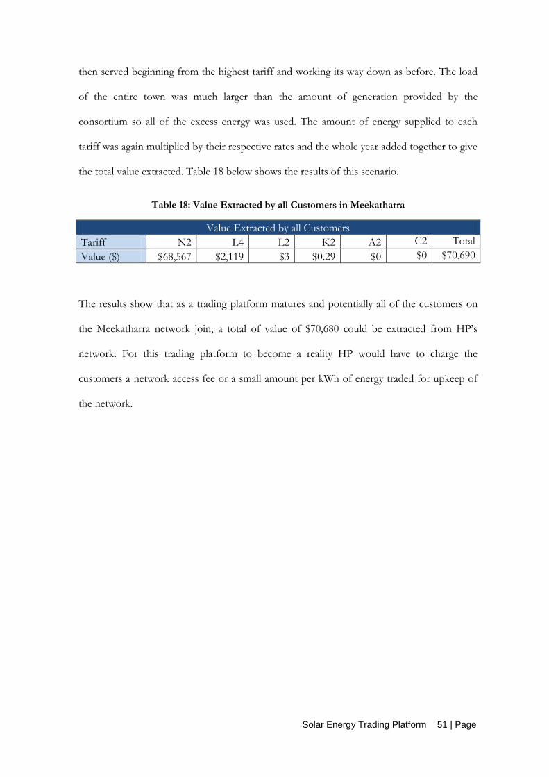
Solar Energy Trading Platform 51 | Page
then served beginning from the highest tariff and working its way down as before. The load
of the entire town was much larger than the amount of generation provided by the
consortium so all of the excess energy was used. The amount of energy supplied to each
tariff was again multiplied by their respective rates and the whole year added together to give
the total value extracted. Table 18 below shows the results of this scenario.
Table 18: Value Extracted by all Customers in Meekatharra
Value Extracted by all Customers
Tariff N2 L4 L2 K2 A2 C2 Total
Value ($) $68,567 $2,119 $3 $0.29 $0 $0 $70,690
The results show that as a trading platform matures and potentially all of the customers on
the Meekatharra network join, a total of value of $70,680 could be extracted from HP’s
network. For this trading platform to become a reality HP would have to charge the
customers a network access fee or a small amount per kWh of energy traded for upkeep of
the network.
52 | Page Conclusion
6.0 Conclusion
6.1 Customer Summary
Attaining correct and complete load profile data for each of the customers formed a greater
challenge than anticipated at this stage of HP’s AMI deployment; however, satisfactory
approximations were achieved through careful and considered data manipulation. The
HOMER modelling was successfully completed using the load profile data and real world
information for the majority of inputs, yielding hourly energy flow results for each of the 13
individual arrays within the virtual solar farm.
These results were extracted and used within the developed Excel spreadsheet to attain each
of the customer’s financial position in a number of different scenarios.
The scenarios included the customer’s financial situation with regards to NPV, IRR and
simple payback with:
- Only the solar array
- Solar array and self-bought solar smoothing battery system
- Solar array and solar smoothing fee, payed to HP for a smoothing service
Sensitivity analyses were also performed on the cost of the array, the solar smoothing
battery, the solar smoothing fee and the feed in tariff to better understand how changing
circumstances will affect the customer’s financial outcomes. This process concluded that for
a number of customers this investment would not be favourable; however, the project
continued for the remaining financially viable customers.

Conclusion 53 | Page
6.2 Horizon Power Summary
The requirements of the solar smoothing battery were developed in accordance to HP’s
guidelines so that the system would meet the stipulated allowable ramp rates. These initial
requirements were then tempered through DIgSILENT PowerFactory simulations of
Meekatharra’s network, including the virtual solar farm and smoothing battery, performed by
HP’s engineering team, to arrive at an optimised solution. This optimum solution was
capable of maintaining grid stability within the network in the worst case scenario that is
likely to occur, whilst being as economical as possible.
The price estimate for the battery, provided by HP, was used in excel to estimate a charge
that would recuperate HP’s invest within the lifetime of the battery system. This was defined
as achieving an NPV of $0. The charge was then included in the customers finances and it
was found that the impact was unacceptable; leading to a sensitivity of the battery price and
charge. The outcomes of this process showed that until a battery system can be installed for
roughly one third of the estimated price the cost cannot be passed on to customers in the
form of a solar smoothing charge.
6.3 Solar Trading Platform Summary
Preliminary research and development was completed for a solar trading platform
culminating in two possible solar trading platform scenarios. These scenarios were modelled
within Excel using the outputs gained from HOMER and the network load profile supplied
by HP to achieve real world results. This allowed the value, in dollars, that such a trading
platform would extract from HP’s network to be quantified. Both if only the current
consortium members were trading and once the platform has matured and all customers on
the Meekatharra network are involved.

54 | Page Conclusion
6.4 Future Work
The customer load profiles used in the HOMER modelling were not a complete year as the
AMI had only been installed for six months at this stage. Once a complete year has elapsed
the models should be re-run with the updated profiles and the outputs compared. If a large
discrepancy is found the energy flow information within the financial modelling can be
updated and the viability of the project reassessed if necessary. By this time the price of
batteries would have fallen, dramatically changing the economic outcomes.
Minor improvements to the HOMER models can be made in the future if the information
becomes available, such as the pitch of the roofs that arrays will be installed on.
As the trading platform is further developed and the exact method of trading is determined
the model should be updated to ensure that it accurately simulates this. The model can be
used to develop possible fees or charges for customers to use HP’s network and assess the
impact this will have on HP. These fees and charges should also be included in the customer
financial models to determine how they are affected and if the price is fair.

References 55 | Page
7.0 References
[1] Horizon Power, “Horizon Power - About us,” Horizon Power, 2016. [Online]. Available:
https://horizonpower.com.au/about-us/overview/who-we-are/. [Accessed October 2016].
[2] Horizon Power, “horizonpower,” [Online]. Available:
http://www.bing.com/images/search?q=horizon+power+about+us&view=detailv2&id=930D2
61291021FB6DFF5F6DB967D264AACA9E671&selectedindex=1&ccid=cux7MYit&simid=60
8001210909986398&thid=OIP.M72ec7b3188addcaa26660794705d31b6o0&mode=overlay
&first=1. [Accessed September 2016].
[3] Australian Bureau of Statistics, “Censusdata,” 9 September 2016. [Online]. Available:
http://censusdata.abs.gov.au/census_services/getproduct/census/2011/quickstat/LGA55250
?opendocument&navpos=220. [Accessed September 2016].
[4] Australian Government Bureau of Meteorology, “Climate Data Online,” September 2016.
[Online]. Available: http://www.bom.gov.au/climate/averages/tables/cw_007045.shtml.
[Accessed September 2016].
[5] Horizon Power, Meekatharra Solar Project_Horizon Power Application_v1.0, Perth: Horizon
Power, 2015.
[6] Horizon Power, “Generation Management,” 2016. [Online]. Available:
http://horizonpower.com.au/being-energy-efficient/solar/generation-management/.
[Accessed August 2016].
[7] Horizon Power, “Generation Management - Technical Requirements,” 25 September 2014.
[Online]. Available: http://horizonpower.com.au/media/1121/technical-requirements-for-
renewable-energy-systems-connected-to-the-low-voltage-lv-network-via-inverters.pdf.
[Accessed August 2016].
[8] HOMER Energy, “HOMER Pro Help Manual,” HOMER Energy, Boulder, 2016.
[9] National Renewable Energy Laboratory, “Changing System Parameters,” [Online]. Available:
http://rredc.nrel.gov/solar/calculators/PVWATTS/system.html. [Accessed August 2016].
[10] J. Harburn, “Solar Choice - Solar Panel Tilt and Orientation in Australia,” 7 January 2010.
[Online]. Available: http://www.solarchoice.net.au/blog/solar-panel-tilt-and-orientation-in-
australia/. [Accessed August 2016].
[11] NASA, “Surface Meteorology and Solar Energy,” September 2016. [Online]. Available:
https://eosweb.larc.nasa.gov/cgi-bin/sse/[email protected]+s03. [Accessed
September 2016].
[12] Horizon Power Finance Department, Finances, Perth, 2016.
[13] Australian Taxation Office, “Australian Government - Australian Taxation Office,” 17 October
2016. [Online]. Available: https://www.ato.gov.au/rates/company-tax/. [Accessed September
2016].

56 | Page References
[14] Horizon Power, “Tariff changes effective 1 July 2016,” 30 June 2016. [Online]. Available:
https://horizonpower.com.au/news-events/news/tariff-changes-effective-1-july-2016/.
[Accessed September 2016].
[15] Horizon Power, “Buyback changes 1 July - Questions and answers,” 29 June 2015. [Online].
Available: https://horizonpower.com.au/news-events/news/buyback-changes-1-july-
questions-and-answers/. [Accessed September 2016].
[16] Hanwha Q CELLS Australia Pty Ltd, “Q.PRO-G4.1 255-265 Datasheet,” May 2015. [Online].
Available: file:///C:/Users/32474096/Downloads/Hanwha_Q_CELLS_Data_sheet.pdf.
[Accessed September 2016].
[17] Committee EL-034, Power Quality, AS 61000.3.100-2011 Limits - Steady state voltage limits
in public electricity systems, Standards Australia, 2011.
[18] R. Martin, “MIT Technology Review,” 29 December 2015. [Online]. Available:
https://www.technologyreview.com/s/544471/renewable-energy-trading-launched-in-
germany/. [Accessed October 2016].
[19] S. Vorrath, “Reneweconomy,” 12 August 2016. [Online]. Available:
http://reneweconomy.com.au/2016/bitcoin-inspired-peer-to-peer-solar-trading-trial-kicks-off-
in-perth-29362. [Accessed September 2016].
[20] B. Tirpak, “Youtube,” The Economist, 17 April 2013. [Online]. Available:
https://www.youtube.com/watch?v=_RNEv5EKUvQ. [Accessed November 2016].
[21] S. Lacey, “Greentech Media,” 4 March 2014. [Online]. Available:
https://www.greentechmedia.com/articles/read/this-is-what-the-utility-death-spiral-looks-like.
[Accessed October 2016].
[22] R. A. Luca Tasquier, “An Agent-Based Collaborative Platform for the Optimised Trading of
Renewable Energy within a Community,” Journal of Telecommunications and Information
Technology, Aversa, 2014.
[23] DIgSILENT, “PowerFactory User Manual,” DIgSILENT, Gomaringen, 2016.
[24] Murdoch University, “ENG470 Engineering Honours Thesis,” 22 June 2015. [Online].
Available:
https://moodleprod.murdoch.edu.au/pluginfile.php/384368/mod_resource/content/3/2015DE
2%20Plan%20and%20Progress%20Report%20FAQ.pdf. [Accessed August 2016].
[25] Meekatharra Accommodation Centre, “Features and Facilities,” [Online]. Available:
http://www.meekatharraaccommodation.com.au/uploads/2/5/8/3/25839954/3092013_orig.jp
g. [Accessed September 2016].

Appendices 57 | Page
8.0 Appendices
8.1 Appendix A
The required results from the HOMER Energy modelling are shown here. The results are
the annual energy generated, annual energy exported, annual energy consumed internally, %
of self-consumption and the percent fed into the grid.
Table 19: HOMER Modelling Outputs for all Customers
Customer One Customer Eight
HOMER Output Amount in kWh HOMER Output Amount in kWh
Annual energy generated 108,298 Annual energy generated 48,054
Annual energy exported 108,268 Annual energy exported 14,958
Annual energy consumed internally 30 Annual energy consumed internally 33,096
% of consumption 0.03% % of consumption 68.87%
% fed into grid 99.97% % fed into grid 31.13%
Customer Two Customer Nine
HOMER Output Amount in kWh HOMER Output Amount in kWh
Annual energy generated 84,911 Annual energy generated 21,609
Annual energy exported 21,739 Annual energy exported 0
Annual energy consumed internally 63,172 Annual energy consumed internally 21,609
% of consumption 74.40% % of consumption 100.00%
% fed into grid 25.60% % fed into grid 0.00%
Customer Three Customer Ten
HOMER Output Amount in kWh HOMER Output Amount in kWh
Annual energy generated 150,235 Annual energy generated 21,624
Annual energy exported 8,308 Annual energy exported 13,228
Annual energy consumed internally 141,927 Annual energy consumed internally 8,396
% of consumption 94.47% % of consumption 38.83%
% fed into grid 5.53% % fed into grid 61.17%
Customer Four Customer Eleven
HOMER Output Amount in kWh HOMER Output Amount in kWh
Annual energy generated 31,235 Annual energy generated 35,632
Annual energy exported 26,076 Annual energy exported 29,786
Annual energy consumed internally 5,159 Annual energy consumed internally 5,846
% of consumption 16.52% % of consumption 16.41%
% fed into grid 83.48% % fed into grid 83.59%
Customer Five Customer Twelve
HOMER Output Amount in kWh HOMER Output Amount in kWh
Annual energy generated 38,443 Annual energy generated 26,632
Annual energy exported 4,902 Annual energy exported 24,830

58 | Page Appendices
Annual energy consumed internally 33,541 Annual energy consumed internally 1,802
% of consumption 87.25% % of consumption 6.77%
% fed into grid 12.75% % fed into grid 93.23%
Customer Six Customer Thirteen
HOMER Output Amount in kWh HOMER Output Amount in kWh
Annual energy generated 13,215 Annual energy generated 30,559
Annual energy exported 9,716 Annual energy exported 16,240
Annual energy consumed internally 3,499 Annual energy consumed internally 14,319
% of consumption 26.48% % of consumption 46.86%
% fed into grid 73.52% % fed into grid 53.14%
Customer Seven
HOMER Output Amount in kWh
Annual energy generated 100,598
Annual energy exported 47,132
Annual energy consumed internally 53,466
% of consumption 53.15%
% fed into grid 46.85%
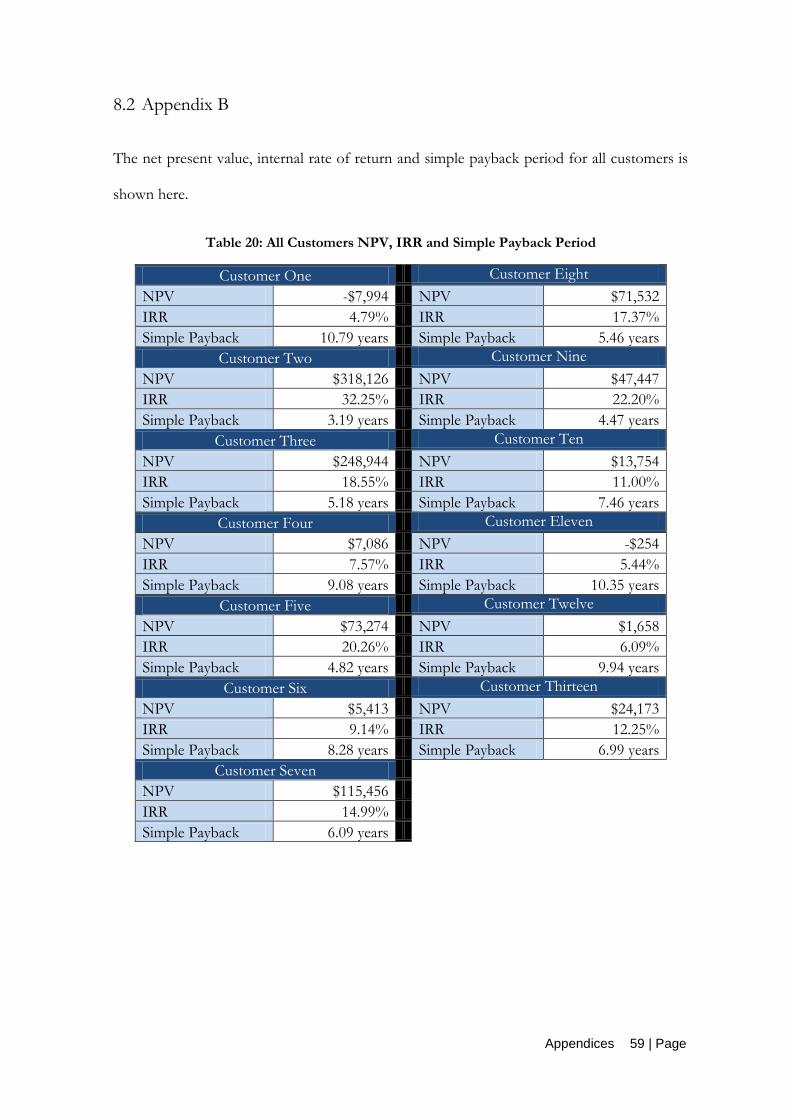
Appendices 59 | Page
8.2 Appendix B
The net present value, internal rate of return and simple payback period for all customers is
shown here.
Table 20: All Customers NPV, IRR and Simple Payback Period
Customer One Customer Eight
NPV -$7,994 NPV $71,532
IRR 4.79% IRR 17.37%
Simple Payback 10.79 years Simple Payback 5.46 years
Customer Two Customer Nine
NPV $318,126 NPV $47,447
IRR 32.25% IRR 22.20%
Simple Payback 3.19 years Simple Payback 4.47 years
Customer Three Customer Ten
NPV $248,944 NPV $13,754
IRR 18.55% IRR 11.00%
Simple Payback 5.18 years Simple Payback 7.46 years
Customer Four Customer Eleven
NPV $7,086 NPV -$254
IRR 7.57% IRR 5.44%
Simple Payback 9.08 years Simple Payback 10.35 years
Customer Five Customer Twelve
NPV $73,274 NPV $1,658
IRR 20.26% IRR 6.09%
Simple Payback 4.82 years Simple Payback 9.94 years
Customer Six Customer Thirteen
NPV $5,413 NPV $24,173
IRR 9.14% IRR 12.25%
Simple Payback 8.28 years Simple Payback 6.99 years
Customer Seven
NPV $115,456
IRR 14.99%
Simple Payback 6.09 years

60 | Page Appendices
8.3 Appendix C
The graphical representation of the simple payback period for all customers is shown here.
Figure 10: Customer One Payback Graph
Figure 11: Customer Two Payback Graph
Figure 12: Customer Three Payback Graph

Appendices 61 | Page
Figure 13: Customer Four Payback Graph
Figure 14: Customer Five Payback Graph
Figure 15: Customer Six Payback Graph

62 | Page Appendices
Figure 16: Customer Seven Payback Graph
Figure 17: Customer Eight Payback Graph
Figure 18: Customer Nine Payback Graph

Appendices 63 | Page
Figure 19: Customer Ten Payback Graph
Figure 20: Customer Eleven Payback Graph
Figure 21: Customer Twelve Payback Graph

64 | Page Appendices
Figure 22: Customer Thirteen Payback Graph

Appendices 65 | Page
8.4 Appendix D
The results for the price of PV per KW sensitivity analysis for all customers are shown here.
Table 21: Cost of System Sensitivity Analysis Results for all Customers
Customer One
Price of Solar ($/kW) $ 2,500 $2,000 $1,500 $1,000
NPV -$7,994 $32,538 $73,070 $113,602
IRR 4.79% 8.86% 14.75% 25.00%
Payback (Years) 10.79 8.41 6.16 4.03
Customer Two
Price of Solar ($/kW) $ 2,500 $2,000 $1,500 $1,000
NPV $318,126 $349,657 $381,189 $412,720
IRR 32.25% 40.80% 54.69% 82.04%
Payback (Years) 3.19 2.54 1.90 1.26
Customer Three
Price of Solar ($/kW) $ 2,500 $2,000 $1,500 $1,000
NPV $248,944 $305,213 $361,482 $417,751
IRR 18.55% 24.45% 33.67% 51.21%
Payback (Years) 5.18 4.11 3.06 2.03
Customer Four
Price of Solar ($/kW) $ 2,500 $2,000 $1,500 $1,000
NPV $7,086 $18,787 $30,488 $42,190
IRR 7.57% 11.92% 18.34% 29.76%
Payback (Years) 9.08 7.11 5.23 3.44
Customer Five
Price of Solar ($/kW) $ 2,500 $2,000 $1,500 $1,000
NPV $73,274 $87,675 $102,076 $116,477
IRR 20.26% 26.45% 36.19% 54.85%
Payback (Years) 4.82 3.83 2.86 1.90
Customer Six
Price of Solar ($/kW) $ 2,500 $2,000 $1,500 $1,000
NPV $5,413 $10,363 $15,314 $20,264
IRR 9.14% 13.67% 20.43% 32.59%
Payback (Years) 8.28 6.50 4.79 3.16
Customer Seven
Price of Solar ($/kW) $ 2,500 $2,000 $1,500 $1,000
NPV $115,456 $152,812 $190,168 $227,524
IRR 14.99% 20.32% 28.52% 43.85%
Payback (Years) 6.09 4.81 3.57 2.37
Customer Eight
Price of Solar ($/kW) $ 2,500 $2,000 $1,500 $1,000
NPV $71,532 $89,534 $107,535 $125,537

66 | Page Appendices
IRR 17.37% 23.07% 31.95% 48.73%
Payback (Years) 5.46 4.32 3.22 2.13
Customer Nine
Price of Solar ($/kW) $ 2,500 $2,000 $1,500 $1,000
NPV $47,447 $55,542 $63,637 $71,732
IRR 22.20% 28.74% 39.10% 59.08%
Payback (Years) 4.47 3.55 2.65 1.76
Customer Ten
Price of Solar ($/kW) $ 2,500 $2,000 $1,500 $1,000
NPV $13,754 $21,855 $29,956 $38,056
IRR 11.00% 15.76% 22.94% 36.04%
Payback (Years) 7.46 5.87 4.34 2.87
Customer Eleven
Price of Solar ($/kW) $ 2,500 $2,000 $1,500 $1,000
NPV -$254 $14,748 $29,749 $44,750
IRR 5.44% 9.57% 15.58% 26.08%
Payback (Years) 10.35 8.0822757 5.92 3.88
Customer Twelve
Price of Solar ($/kW) $ 2,500 $2,000 $1,500 $1,000
NPV $1,658 $11,559 $21,460 $31,361
IRR 6.09% 10.28% 16.41% 27.18%
Payback (Years) 9.94 7.76634491 5.70 3.73
Customer Thirteen
Price of Solar ($/kW) $ 2,500 $2,000 $1,500 $1,000
NPV $24,173 $35,574 $46,975 $58,376
IRR 12.25% 17.18% 24.66% 38.42%
Payback (Years) 6.99 5.5026169 4.08 2.70

Appendices 67 | Page
8.5 Appendix E
The results for the customer bought solar smoothing batteries sensitivity analysis for all
customers are shown here.
Table 22: Customer Bought Solar Smoothing Sensitivity Analysis Results for all Customers
Customer One
Customer Bought Smoothing ($/kW) $0 $500 $1,000 $1,500 $2,000
NPV -$7,994 -$48,526 -$89,057 -$129,589 -$170,121
IRR 4.79% 1.70% -0.81% -2.94% -4.80%
Payback (Years) 10.79 13.29 15.91 18.65 21.50
Customer Two
Customer Bought Smoothing ($/kW) $0 $500 $1,000 $1,500 $2,000
NPV $318,126 $286,595 $255,064 $223,533 $192,002
IRR 32.25% 26.36% 21.99% 18.57% 15.79%
Payback (Years) 3.19 3.84 4.50 5.18 5.86
Customer Three
Customer Bought Smoothing ($/kW) $0 $500 $1,000 $1,500 $2,000
NPV $248,944 $192,675 $136,405 $80,136 $23,867
IRR 18.55% 14.34% 11.10% 8.50% 6.32%
Payback (Years) 5.18 6.29 7.42 8.59 9.80
Customer Four
Customer Bought Smoothing ($/kW) $0 $500 $1,000 $1,500 $2,000
NPV $7,086 -$4,615 -$16,316 -$28,017 -$39,718
IRR 7.57% 4.31% 1.70% -0.47% -2.35%
Payback (Years) 9.08 11.14 13.29 15.52 17.85
Customer Five
Customer Bought Smoothing ($/kW) $0 $500 $1,000 $1,500 $2,000
NPV $73,274 $58,872 $44,471 $30,070 $15,669
IRR 20.26% 15.85% 12.50% 9.80% 7.57%
Payback (Years) 4.82 5.85 6.90 7.98 9.08
Customer Six
Customer Bought Smoothing ($/kW) $0 $500 $1,000 $1,500 $2,000
NPV $5,413 $462 -$4,488 -$9,439 -$14,389
IRR 9.14% 5.77% 3.10% 0.88% -1.03%
Payback (Years) 8.28 10.14 12.07 14.08 16.17
Customer Seven
Customer Bought $0 $500 $1,000 $1,500 $2,000

68 | Page Appendices
Smoothing ($/kW)
NPV $115,456 $78,100 $40,744 $3,387 -$33,969
IRR 14.99% 11.13% 8.14% 5.70% 3.65%
Payback (Years) 6.09 7.41 8.78 10.18 11.64
Customer Eight
Customer Bought Smoothing ($/kW) $0 $500 $1,000 $1,500 $2,000
NPV $71,532 $53,531 $35,529 $17,527 -$474
IRR 17.37% 13.28% 10.13% 7.58% 5.45%
Payback (Years) 5.46 6.63 7.83 9.07 10.35
Customer Nine
Customer Bought Smoothing ($/kW) $0 $500 $1,000 $1,500 $2,000
NPV $47,447 $47,447 $39,352 $31,257 $23,162
IRR 22.20% 22.20% 17.58% 14.07% 11.27%
Payback (Years) 4.47 4.47 5.41 6.37 7.36
Customer Ten
Customer Bought Smoothing ($/kW) $0 $500 $1,000 $1,500 $2,000
NPV $13,754 $5,653 -$2,447 -$10,548 -$18,649
IRR 11.00% 7.49% 4.72% 2.44% 0.50%
Payback (Years) 7.46 9.12 10.84 12.62 14.47
Customer Eleven
Customer Bought Smoothing ($/kW) $0 $500 $1,000 $1,500 $2,000
NPV -$254 -$15,255 -$30,256 -$45,258 -$60,259
IRR 5.44% 2.31% -0.22% -2.35% -4.22%
Payback (Years) 10.35 12.74 15.24 17.85 20.56
Customer Twelve
Customer Bought Smoothing ($/kW) $0 $500 $1,000 $1,500 $2,000
NPV $1,658 -$8,243 -$18,144 -$28,045 -$37,945
IRR 6.09% 2.92% 0.37% -1.78% -3.64%
Payback (Years) 9.94 12.22 14.60 17.09 19.68
Customer Thirteen
Customer Bought Smoothing ($/kW) $0 $500 $1,000 $1,500 $2,000
NPV $24,173 $12,772 $1,371 -$10,030 -$21,431
IRR 12.25% 8.63% 5.80% 3.48% 1.50%
Payback (Years) 6.99 8.52 10.12 11.77 13.47

Appendices 69 | Page
8.6 Appendix F
The results for the solar smoothing charge sensitivity analysis for all customers are shown
here. Any cells showing #NUM indicate that the solar smoothing charge in this case was
greater than any benefit derived from the array; an IRR therefore cannot be calculated.
Table 23: Solar Smoothing Charge Sensitivity Analysis Results for all Customers
Customer One
Solar Smoothing Service ($/kW. Month) $0.00 $62.80 $118.22 $229.06 $339.91
NPV -$7,994 -$52,539 -$91,846 -$170,462 -$249,078
IRR 4.79% 0.38% -4.63% #NUM! #NUM!
Payback (Years) 10.79 14.58 21.88 26.00 26.00
Customer Two
Solar Smoothing Service ($/kW. Month) $0.00 $62.80 $118.22 $229.06 $339.91
NPV $318,126 $270,676 $228,805 $145,062 $61,319
IRR 32.25% 28.86% 25.78% 19.28% 11.98%
Payback (Years) 3.19 3.53 3.90 4.96 6.90
Customer Three
Solar Smoothing Service ($/kW. Month) $0.00 $62.80 $118.22 $229.06 $339.91
NPV $248,944 $182,126 $123,164 $5,241 -$112,683
IRR 18.55% 15.44% 12.52% 5.84% -3.51%
Payback (Years) 5.18 5.94 6.84 9.94 21.16
Customer Four
Solar Smoothing Service ($/kW. Month) $0.00 $62.80 $118.22 $229.06 $339.91
NPV $7,086 -$9,053 -$23,295 -$51,779 -$80,263
IRR 7.57% 2.58% -3.11% #NUM! #NUM!
Payback (Years) 9.08 12.47 19.28 26.00 26.00
Customer Five
Solar Smoothing Service ($/kW. Month) $0.00 $62.80 $118.22 $229.06 $339.91
NPV $73,274 $55,117 $39,094 $7,050 -$24,995
IRR 20.26% 17.04% 14.03% 7.23% -2.06%
Payback (Years) 4.82 5.52 6.34 9.11 18.10
Customer Six
Solar Smoothing Service ($/kW. Month) $0.00 $62.80 $118.22 $229.06 $339.91
NPV $5,413 -$1,043 -$6,740 -$18,134 -$29,527
IRR 9.14% 4.74% 0.03% -22% #NUM!
Payback (Years) 8.28 10.79 14.96 26.00 26.00

70 | Page Appendices
Customer Seven
Solar Smoothing Service ($/kW. Month) $0.00 $62.80 $118.22 $229.06 $339.91
NPV $115,456 $66,957 $24,159 -$61,435 -$147,029
IRR 14.99% 11.32% 7.73% -1% #NUM!
Payback (Years) 6.09 7.31 8.91 16.91 26.00
Customer Eight
Solar Smoothing Service ($/kW. Month) $0.00 $62.80 $118.22 $229.06 $339.91
NPV $71,532 $47,323 $25,960 -$16,766 -$59,492
IRR 17.37% 13.75% 10.28% 2% -15.59%
Payback (Years) 5.46 6.44 7.70 13.02 26.00
Customer Nine
Solar Smoothing Service ($/kW. Month) $0.00 $62.80 $118.22 $229.06 $339.91
NPV $47,447 $37,360 $28,459 $10,656 -$7,146
IRR 22.20% 19.11% 16.25% 10% 2.00%
Payback (Years) 4.47 5.05 5.70 7.79 12.81
Customer Ten
Solar Smoothing Service ($/kW. Month) $0.00 $62.80 $118.22 $229.06 $339.91
NPV $13,754 $3,667 -$5,234 -$23,037 -$40,839
IRR 11.00% 7.07% 3.07% -9% #NUM!
Payback (Years) 7.46 9.31 12.02 26.00 26.00
Customer Eleven
Solar Smoothing Service ($/kW. Month) $0.00 $62.80 $118.22 $229.06 $339.91
NPV -$254 -$21,235 -$39,749 -$76,779 -$113,808
IRR 5.44% -0.17% -7.22% #NUM! #NUM!
Payback (Years) 10.35 15.19 26.00 26.00 26.00
Customer Twelve
Solar Smoothing Service ($/kW. Month) $0.00 $62.80 $118.22 $229.06 $339.91
NPV $1,658 -$14,481 -$28,723 -$57,207 -$85,691
IRR 6.09% -0.40% -9.28% #NUM! #NUM!
Payback (Years) 9.94 15.45 26.00 26.00 26.00
Customer Thirteen
Solar Smoothing Service ($/kW. Month) $0.00 $62.80 $118.22 $229.06 $339.91
NPV $24,173 $8,033 -$6,209 -$34,693 -$63,177
IRR 12.25% 7.91% 3.46% -11% #NUM!
Payback (Years) 6.99 8.85 11.69 26.00 26.00

Appendices 71 | Page
8.7 Appendix G
The yearly net cash flow for HP, caused by the installation of the virtual solar farm, over the
15 years of the project is shown here.
Table 24: Horizon Power Yearly Net Cash Flow
Horizon Power Finances Year 1 Year 2 Year 3 Year 4 Year 5
Net Cash Flow -$33,353 -$34,536 -$35,759 -$37,023 -$37,594
Horizon Power Finances Year 6 Year 7 Year 8 Year 9 Year 10
Net Cash Flow -$38,171 -$38,753 -$39,340 -$39,933 -$40,530
Horizon Power Finances Year 11 Year 12 Year 13 Year 14 Year 15
Net Cash Flow -$41,133 -$41,740 -$42,352 -$42,968 -$43,589

72 | Page Appendices
8.8 Appendix H
Permission to use figure 1, Horizon Power Supply Area, given by the appropriate HP staff
member is shown here. The following is the email chain pertaining to the use of the graphic.
From: Andrew Riches
Sent: Tuesday, 25 October 2016 4:58 PM To: Kelli Friar
CC: Pierce Trinkl
Subject: Horizon Power Graphic
No problem with using the map and please let me know if you require it in an alert at format.
Sent from my iPhone
On 25 Oct. 2016, at 3:00 pm, Kelli Friar <[email protected]> wrote:
Hi Andrew,
Pierce is a student working with us. Can he use the below image in his thesis
cheers
<image003.png> Kelli Friar
Strategic Projects Manager
T: (08) 6310 1502 | 18 Brodie Hall Drive, Bentley WA 6102
M: 0429 889 506 | [email protected]
horizonpower.com.au | Facebook | Twitter
<image001.jpg>
From: Pierce Trinkl
Sent: Tuesday, 25 October 2016 2:43 PM To: Kelli Friar
Subject: Horizon Power Graphic