MEDIEVAL WARFARE ON THE GRID

by

PHILIP SCOTT MURGATROYD

A thesis submitted to the University of Birmingham

for the degree of DOCTOR OF PHILOSOPHY

Institute of Archaeology and AntiquityCollege of Arts and Law

The University of BirminghamJanuary 2012

University of Birmingham Research Archive

e-theses repository This unpublished thesis/dissertation is copyright of the author and/or third parties. The intellectual property rights of the author or third parties in respect of this work are as defined by The Copyright Designs and Patents Act 1988 or as modified by any successor legislation. Any use made of information contained in this thesis/dissertation must be in accordance with that legislation and must be properly acknowledged. Further distribution or reproduction in any format is prohibited without the permission of the copyright holder.

ABSTRACT

Although historical studies are frequently perceived as clear narratives defined by a series

of fixed events; in reality, even where critical historical events may be identified, historic

documentation frequently lacks corroborative detail to support verifiable interpretation.

Consequently, interpretation rarely rises above the level of unproven assertion and is rarely tested

against a range of evidence. Agent-based simulation can provide an opportunity to break these

cycles of academic claim and counter-claim.

This thesis discusses the development of an agent-based simulation designed to

investigate medieval military logistics so that new evidence may be generated to supplement

existing historical analysis. It uses as a case-study the Byzantine army’s march to the battle of

Manzikert (AD 1071), a key event in medieval history. It describes the design and implementation

of a series of agent-based models and presents the results of these models. The analysis of these

results shows that agent-based modelling is a powerful tool in investigating the practical

limitations faced by medieval armies on campaign.

ACKNOWLEDGEMENTS

This research would not have been possible without the funding provided by an AHRC-

EPSRC-JISC e-Science grant and I would like to thank Vince Gaffney and Georgios

Theodoropoulos for applying for this grant and starting the Medieval Warfare on the Grid

project. Vince especially deserves thanks for supervising my PhD and helping to make it

presentable. Thanks also go to the University of Birmingham College of Arts and Law who also

provided funding for the final year. I would also like to thank John Haldon for his help with the

historical data and his role in the creation of the project as a whole and to Helen Gaffney for

putting together the original bibliography and GIS data, without all these people and institutions

this PhD would not exist.

I would also like to thank those people at the university who gave valuable help and

advice. John Carman, Archie Dunn, Warren Eastwood, Henry Chapman, Eugene Ch'ng and

Mike White all contributed their valuable knowledge when needed. Thanks also go to Julian D

Richards and Damian Robinson who helped with my application for this PhD, and to Rick Jones

for his help in Bradford and Pompeii. The staff and students in the VISTA centre have all

provided useful help and support along the way, along with a friendly and enjoyable working

environment. Simon Fitch and Paul Hatton have particularly helped with technical issues.

Software advice from first Rob Minson and then Bart Craenen has also helped in producing a

series of models that actually work pretty well, something unlikely if I'd been left to my own

devices. Any errors are, of course, mine.

Finally I wouldn't have been able to have done this without the help and support of my

parents and of Jenn who has made the whole time spent on this thesis a much happier one than

it would otherwise have been.

Table of Contents1 Introduction................................................................................................................................................1

1.1 Introduction.........................................................................................................................................11.2 The Manzikert Campaign..................................................................................................................3

1.2.1 The Importance of Manzikert.................................................................................................71.2.2 The Campaign.............................................................................................................................81.2.3 What is Missing?.........................................................................................................................8

1.3 The Need to Model..........................................................................................................................111.3.1 Why Can This Not Be Filled With Conventional Research?............................................121.3.2 Adding Complexity to Engels and Pryor.............................................................................131.3.3 Individuals.................................................................................................................................14

1.4 There is a Technology That Can Do This, ABM........................................................................151.4.1 The History of ABM...............................................................................................................171.4.2 ABM in Archaeology...............................................................................................................181.4.3 Is the Byzantine Army a Complex System?.........................................................................201.4.4 The Limitations of ABM........................................................................................................211.4.5 The Potential of ABM............................................................................................................22

1.5 Summary.............................................................................................................................................242 The ABM Design......................................................................................................................................25

2.1 Introduction.......................................................................................................................................252.2 Modelling Considerations................................................................................................................26

2.2.1 What We Want to Find Out...................................................................................................272.2.2 Appropriate Abstraction.........................................................................................................282.2.3 Stochastic Elements.................................................................................................................292.2.4 Issues With the Environment................................................................................................292.2.5 Issues With the Agents............................................................................................................302.2.6 What We Want From the Output..........................................................................................30

2.3 The Agents.........................................................................................................................................312.3.1 The Sources...............................................................................................................................31

2.3.1.1 The Army Would Have Picked Up Troops Along the Way.....................................342.3.1.2 Supplies Would Also Have Been Picked Up Along the Way...................................342.3.1.3 There Would Have Been a Route Planned in Advance.............................................342.3.1.4 The Army Would Have a Regular Routine For Marching........................................352.3.1.5 The Army Would Have a Set Order of March...........................................................362.3.1.6 The Army Would Have Had a Consistent and Organised Method for Setting up Camp...............................................................................................................................................392.3.1.7 The Emperor Makes all the Strategic Decisions........................................................402.3.1.8 The Length of a Daily March Must be Flexible and Practical.................................402.3.1.9 How Did it Move?...........................................................................................................42

2.4 The Art of Marching........................................................................................................................432.4.1 The Size of the Column..........................................................................................................45

2.4.1.1 Individual Units................................................................................................................462.4.1.2 The Whole Army.............................................................................................................46

i

2.4.1.3 The Lengthening of the Column..................................................................................462.4.2 The Speed of the Army..........................................................................................................47

2.4.2.1 Cavalry and Baggage.......................................................................................................482.4.2.2 Forced Marches................................................................................................................482.4.2.3 Barriers to Progress.........................................................................................................49

2.4.3 How the Army Organises its Movement.............................................................................492.4.3.1 Breaking Camp.................................................................................................................502.4.3.2 Marching Formations......................................................................................................502.4.3.3 Splitting the Column......................................................................................................512.4.3.4 Resting on the March......................................................................................................512.4.3.5 Navigation Aids...............................................................................................................522.4.3.6 If You Fail to Plan... .......................................................................................................52

2.4.4 Caring for the Soldiers and Animals.....................................................................................532.4.4.1 Food & Water...................................................................................................................542.4.4.2 Other Hazards..................................................................................................................552.4.4.3 Animal Care......................................................................................................................55

2.4.5 General Advice.........................................................................................................................562.4.6 Conclusions...............................................................................................................................572.4.7 Which Elements are Necessary for Which Aspects of the Project?...............................592.4.8 The Army's Behaviour.............................................................................................................592.4.9 Agent Organisation and Types...............................................................................................60

2.4.9.1 The Emperor and His Retinue......................................................................................602.4.9.2 Generals and Bureaucrats...............................................................................................602.4.9.3 Household Troops...........................................................................................................612.4.9.4 Thematic Tagmata...........................................................................................................612.4.9.5 Turkic Nomads................................................................................................................612.4.9.6 Frankish Mercenaries......................................................................................................612.4.9.7 Support..............................................................................................................................62

2.4.10 Agent Types............................................................................................................................622.4.10.1 Human Agents...............................................................................................................632.4.10.2 Animal Agents................................................................................................................63

2.4.11 Agent Architecture.................................................................................................................642.4.11.1 Inbox................................................................................................................................642.4.11.2 Plan Queue.....................................................................................................................642.4.11.3 Perception Base..............................................................................................................642.4.11.4 Attributes........................................................................................................................642.4.11.5 Behaviours......................................................................................................................65

2.5 Human Agents: Attributes..............................................................................................................652.6 Human Agents: Behaviours............................................................................................................66

2.6.1.1 Health................................................................................................................................662.6.1.2 Emperor............................................................................................................................682.6.1.3 General..............................................................................................................................702.6.1.4 Quartermaster..................................................................................................................702.6.1.5 Surveyor.............................................................................................................................712.6.1.6 Byzantine Cavalry............................................................................................................742.6.1.7 Byzantine Infantry...........................................................................................................752.6.1.8 Turkic Cavalry..................................................................................................................75

ii

2.6.1.9 Frankish Cavalry..............................................................................................................752.6.1.10 Servant.............................................................................................................................75

2.7 Movement..........................................................................................................................................752.7.1 Macro-Scale Movement...........................................................................................................772.7.2 Micro-Scale Movement...........................................................................................................782.7.3 Intermediate-Scale Movement...............................................................................................78

2.8 Calorie Expenditure..........................................................................................................................792.9 The Environment.............................................................................................................................82

2.9.1 What Was the Environment Like?........................................................................................822.9.2 Environmental Slices...............................................................................................................85

2.9.2.1 Height – A Digital Elevation Model of Anatolia.......................................................852.9.2.1.1 Resolution.................................................................................................................852.9.2.1.2 Source........................................................................................................................852.9.2.1.3 Format.......................................................................................................................862.9.2.1.4 Effect.........................................................................................................................86

2.9.2.2 Settlement – Indicates Location and Type of Settlement........................................862.9.2.2.1 Resolution.................................................................................................................862.9.2.2.2 Source........................................................................................................................872.9.2.2.3 Format.......................................................................................................................872.9.2.2.4 Effect.........................................................................................................................93

2.9.2.3 Globcover – The European Space Agency's Vegetation Cover Database.............942.9.2.3.1 Resolution.................................................................................................................942.9.2.3.2 Source........................................................................................................................942.9.2.3.3 Format.......................................................................................................................952.9.2.3.4 Effect.........................................................................................................................95

2.9.2.4 Transport – Presence of Roads....................................................................................972.9.2.4.1 Resolution.................................................................................................................972.9.2.4.2 Source........................................................................................................................972.9.2.4.3 Format.......................................................................................................................992.9.2.4.4 Effect.........................................................................................................................99

2.9.2.5 Water – Presence and Type of Water...........................................................................992.9.2.5.1 Source........................................................................................................................992.9.2.5.2 Format.......................................................................................................................992.9.2.5.3 Effect.........................................................................................................................99

2.9.3 Weather Data..........................................................................................................................1002.10 Conclusion.....................................................................................................................................102

3 Implementation.......................................................................................................................................1053.1 Introduction.....................................................................................................................................1053.2 Temporal and Spatial Resolution.................................................................................................1053.3 Building the Model.........................................................................................................................106

3.3.1 Focussing on the Micro-Scale..............................................................................................1073.4 The Simulation Process.................................................................................................................109

3.4.1 The Initialisation File.............................................................................................................1103.4.2 The MWGrid ABM...............................................................................................................115

3.4.2.1 The Main Programme...................................................................................................1153.4.2.1.1 Initialise Environment.........................................................................................1163.4.2.1.2 Initialise Output Files...........................................................................................116

iii

3.4.2.1.3 Calculate Camp Sector Sizes...............................................................................1163.4.2.1.4 Create Central Sector...........................................................................................1163.4.2.1.5 Create Outer Sectors............................................................................................1163.4.2.1.6 Initialise Context..................................................................................................1173.4.2.1.7 Call Step Method of Each Agent......................................................................117

3.4.2.2 The Agents.....................................................................................................................1183.4.2.2.1 HumanAgent.........................................................................................................1183.4.2.2.2 ColumnLeader.......................................................................................................1203.4.2.2.3 Officer.....................................................................................................................1203.4.2.2.4 CavalryOfficer.......................................................................................................1213.4.2.2.5 Soldier.....................................................................................................................1213.4.2.2.6 CavalrySoldier........................................................................................................121

3.4.2.3 Plans and Actions..........................................................................................................1213.4.2.4 Messages..........................................................................................................................1243.4.2.5 Route Planning...............................................................................................................125

3.5 A* Route Planning..........................................................................................................................1263.5.1 Grid Movement......................................................................................................................1293.5.2 Probabilistic RoadMap Movement......................................................................................1303.5.3 Why Not Just A*?..................................................................................................................1313.5.4 What is the Solution?.............................................................................................................132

3.5.4.1 Shuffling..........................................................................................................................1353.5.4.2 The Environment..........................................................................................................137

3.5.4.2.1 SliceMap.................................................................................................................1373.5.4.2.2 SliceArray...............................................................................................................1383.5.4.2.3 PartitionedSliceArray............................................................................................138

3.6 Overall Army Behaviour................................................................................................................1383.6.1 The Dayfile..............................................................................................................................1403.6.2 The Tickfile.............................................................................................................................1423.6.3 Blender.....................................................................................................................................143

3.6.3.1 First Python Script........................................................................................................1433.6.3.2 Second Python Script....................................................................................................145

3.6.4 Blender pre-processing..........................................................................................................1453.6.5 OpenOffice Calc....................................................................................................................146

3.7 Summary..........................................................................................................................................1474 The Day's March Scenarios...................................................................................................................149

4.1 Introduction.....................................................................................................................................1494.1.1 Units of Measurement..........................................................................................................151

4.2 Initial Setup......................................................................................................................................1514.3 Start and Finish Locations............................................................................................................1534.4 Hardware Overview.......................................................................................................................1544.5 The Day's March Scenarios...........................................................................................................155

4.5.1 DM001.....................................................................................................................................1554.5.2 DM002.....................................................................................................................................1564.5.3 DM003.....................................................................................................................................1564.5.4 DM004.....................................................................................................................................1564.5.5 DM005.....................................................................................................................................1574.5.6 DM006 & DM006a................................................................................................................157

iv

4.5.7 DM007.....................................................................................................................................1574.5.8 DM008.....................................................................................................................................1574.5.9 DM009.....................................................................................................................................157

4.6 DM001 - Crowding........................................................................................................................1584.6.1 Introduction............................................................................................................................1584.6.2 Calibration of the Model......................................................................................................1584.6.3 Running of the Model...........................................................................................................1594.6.4 Setup.........................................................................................................................................1604.6.5 Results......................................................................................................................................161

4.6.5.1 Processing Times...........................................................................................................1614.6.5.2 Distance Travelled.........................................................................................................1624.6.5.3 Average Arrival Time in Camp....................................................................................1634.6.5.1 Maximum Column Length...........................................................................................164

4.6.6 DM001 Conclusions..............................................................................................................1654.7 DM002 – Resting on the March...................................................................................................166

4.7.1 Introduction............................................................................................................................1664.7.2 Work Required........................................................................................................................167

4.7.2.1 Fixing Order Problems from DM001........................................................................1674.7.2.2 New Time Handling Procedures................................................................................1684.7.2.3 Better Flocking...............................................................................................................1694.7.2.4 Changes to the Initfile..................................................................................................169

4.7.3 Results......................................................................................................................................1714.7.3.1 Processing Times...........................................................................................................1724.7.3.2 Distance Travelled.........................................................................................................1734.7.3.3 Average Arrival Time in Camp....................................................................................1734.7.3.4 Maximum Column Length...........................................................................................1744.7.3.5 Rest Ticks........................................................................................................................176

4.7.4 DM002 Conclusions..............................................................................................................1764.8 DM003 - The Practical Limits of the Day's March Model.....................................................177

4.8.1 Introduction............................................................................................................................1774.8.2 Work Required........................................................................................................................1784.8.3 Results......................................................................................................................................178

4.8.3.1 Processing Times...........................................................................................................1794.8.4 DM003 Conclusions..............................................................................................................179

4.9 DM004 - Effects of Environment Variables on ABM performance....................................1804.9.1 Introduction............................................................................................................................1804.9.2 Brief Overview.......................................................................................................................1814.9.3 Results......................................................................................................................................181

4.9.3.1 Processing Times..........................................................................................................1824.9.4 DM004 Conclusions..............................................................................................................183

4.10 DM005 – Cavalry.........................................................................................................................1834.10.1 Introduction..........................................................................................................................1834.10.2 Work Required......................................................................................................................183

4.10.2.1 Agent Size.....................................................................................................................1834.10.2.2 Agent Speed.................................................................................................................1844.10.2.3 Army Organisation.....................................................................................................1864.10.2.4 Camp Setup..................................................................................................................187

v

4.10.2.1 Weather.........................................................................................................................1894.10.3 Results....................................................................................................................................191

4.10.3.1 Processing Times.........................................................................................................1914.10.3.2 Distance Travelled and Average Rest Ticks............................................................1924.10.3.3 Individual Arrival Time in Camp..............................................................................192

4.10.4 DM005 Conclusions............................................................................................................1984.11 DM006 – The Limits of a Single Column...............................................................................198

4.11.1 Introduction..........................................................................................................................1984.11.1.1 Army Composition.....................................................................................................1994.11.1.2 Setting Off Delays.....................................................................................................1994.11.1.3 Cavalry Speed...............................................................................................................1994.11.1.4 March Spacing..............................................................................................................199

4.11.2 Work Required......................................................................................................................2004.11.2.1 Setting Off....................................................................................................................200

4.11.3 Results....................................................................................................................................2014.11.3.1 Army Composition.....................................................................................................2024.11.3.2 Setting Off Delays......................................................................................................2034.11.3.3 Cavalry Speed...............................................................................................................206

4.11.4 Data........................................................................................................................................2064.11.4.1 The Effects of Increased Cavalry Speed in Cavalry-Only Forces......................206

4.11.5 The Effects of Increased Cavalry Speed in Mixed Forces...........................................2074.11.5.1 March Spacing..............................................................................................................209

4.11.6 DM006 Conclusion.............................................................................................................2124.12 DM006a – The Limits of a Single Column.............................................................................213

4.12.1 Introduction..........................................................................................................................2134.12.2 Data........................................................................................................................................2144.12.3 Results....................................................................................................................................215

4.12.3.1 6 Miles...........................................................................................................................2154.12.3.2 12 Miles.........................................................................................................................2154.12.3.3 15 Miles.........................................................................................................................216

4.12.4 DM006a Conclusions..........................................................................................................2164.13 DM007 – Multiple Columns.......................................................................................................216

4.13.1 Introduction..........................................................................................................................2164.13.2 Work Required......................................................................................................................2174.13.3 Data........................................................................................................................................2214.13.4 Results....................................................................................................................................222

4.13.4.1 6 Miles...........................................................................................................................2224.13.4.2 12 Miles.........................................................................................................................2254.13.4.3 15 miles.........................................................................................................................228

4.13.5 DM007 Conclusions............................................................................................................2304.14 DM008 – The March to Manzikert...........................................................................................233

4.14.1 Introduction..........................................................................................................................2334.14.2 Work Required......................................................................................................................234

4.14.2.1 Route.............................................................................................................................2344.14.2.2 Army Composition.....................................................................................................2344.14.2.3 Weather and Daylight.................................................................................................2364.14.2.4 Timing...........................................................................................................................236

vi

4.14.2.5 Movement Costs..........................................................................................................2384.14.2.6 Health............................................................................................................................2384.14.2.7 Nicomedia to Malagina..............................................................................................2404.14.2.8 Malagina to Dorylaion................................................................................................244

4.14.2.8.1 Cross Section of the Day's March...................................................................2454.14.2.8.2 Data.......................................................................................................................246

4.14.2.9 Charsianon to Sebastea...............................................................................................2474.14.2.9.1 Cross Section of the Day's March...................................................................2484.14.2.9.2 Data.......................................................................................................................249

4.14.2.10 Theodosiopolis to Manzikert..................................................................................2504.14.3 DM008 Conclusions............................................................................................................252

4.15 DM009 - Supply............................................................................................................................2534.15.1 Introduction..........................................................................................................................2534.15.2 Data........................................................................................................................................2554.15.3 Cross Section of the March...............................................................................................2584.15.4 Supplies..................................................................................................................................2594.15.5 DM009 Conclusions............................................................................................................260

4.16 Summary........................................................................................................................................2615 Conclusions..............................................................................................................................................263

5.1 Introduction.....................................................................................................................................2635.2 The Art of Marching.....................................................................................................................2635.3 Reuse.................................................................................................................................................2645.4 Applicability of the Project to Other Places and Times..........................................................2655.5 Class Warfare...................................................................................................................................2655.6 What Effect Did the Supply of the Army Have on the Settlements Through Which it Passed?....................................................................................................................................................2675.7 How Did the Army Organisation Affect the Overall Speed?.................................................2695.8 How Our Results Compare With Records of Armies Marching...........................................2715.9 How Do the Size and Composition of the Army Affect the Overall Speed?.....................2725.10 Problems Encountered................................................................................................................2755.11 Future Work...................................................................................................................................2755.12 Summary........................................................................................................................................276

6 Glossary....................................................................................................................................................2787 List of References...................................................................................................................................2798 Appendix 1...............................................................................................................................................283

8.1 ManzikertDaysMarchSP................................................................................................................2839 Appendix 2...............................................................................................................................................291

9.1 HumanAgent...................................................................................................................................291

Table of FiguresFigure 1: Byzantine Anatolia showing the Turkish raids..........................................................................4Figure 2: The modelling process................................................................................................................27Figure 3: March formation in friendly territory (after Haldon, 1999).................................................38Figure 4: The camp, populated by the units from Figure 2...................................................................40

vii

Figure 5: Agent Organisation.....................................................................................................................60Figure 6: Agent architecture........................................................................................................................64Figure 7: Agent health decision making....................................................................................................66Figure 8: General's health decision making process...............................................................................68Figure 9: Emperor's decision making process for each day's march...................................................69Figure 10: Quartermaster's decision making process.............................................................................71Figure 11: Surveyor's decision making process.......................................................................................72Figure 12: Foraging leader's decision making process............................................................................74Figure 13: The three levels of route planning.........................................................................................79Figure 14: Anatolia with the MWGrid environment boundary in red.................................................85Figure 15: ASTER GDEM data for Anatolia..........................................................................................86Figure 16: Settlements from all sources....................................................................................................87Figure 17: The area covered by the TIB maps with the West and East areas of extrapolated data..........................................................................................................................................................................89Figure 18: Settlement data derived from TIB maps................................................................................90Figure 19: Modern settlement data............................................................................................................91Figure 20: Modern settlements split into TIB categories. Orange dots are discarded points.........92Figure 21: ESA Globcover data.................................................................................................................95Figure 22: The roads represented in the ABM........................................................................................97Figure 23: Map of Anatolia from Haldon (1999)...................................................................................98Figure 24: Water data.................................................................................................................................100Figure 25: Location of weather station with the ABM area...............................................................102Figure 26: The intended MWGrid infrastructure (from Murgatroyd et al. 2011)...........................108Figure 27: The simulation process...........................................................................................................110Figure 28: Sample initialisation file data.................................................................................................111Figure 29: Flow of the main programme...............................................................................................115Figure 30: Agent Java class hierarchy......................................................................................................118Figure 31: The HumanAgent step method............................................................................................119Figure 32: A TravelTo symbolic action expands into a series of Moves..........................................122Figure 33: An example of A* in action..................................................................................................127Figure 34: Grid movement........................................................................................................................130Figure 35: PRM movement.......................................................................................................................131Figure 36: Graph showing relationship between heuristic modifier and performance..................134Figure 37: Flowchart detailing dynamic route planning logic.............................................................135Figure 38: Environment class organisation............................................................................................137Figure 39: Sample camp layout with single column waypoints marked............................................140Figure 40: Part of a dayfile from DM007...............................................................................................141Figure 41: Section of a tickfile.................................................................................................................143Figure 42: Output from the first python script showing both sets of art assets.............................144Figure 43: Output from the second python script................................................................................145Figure 44: The dayfile spreadsheet for aggregated data.......................................................................146Figure 45: Sample tabulated aggregate data from the spreadsheet....................................................147Figure 46: Anatolia with the ABM extent marked in red....................................................................153Figure 47: Processing time per run..........................................................................................................162Figure 48: Distance travelled per run......................................................................................................163Figure 49: Arrival times per run...............................................................................................................164Figure 50: Maximum column length by run..........................................................................................165

viii

Figure 51: Key for the graphs of DM002..............................................................................................170Figure 52: DM002 processing times........................................................................................................172Figure 53: DM002 average distances travelled.......................................................................................173Figure 54: DM002 average arrival time at destination camp...............................................................173Figure 55: DM002 maximum column length........................................................................................174Figure 56: DM002 tick of maximum column length...........................................................................175Figure 57: DM002 average rest ticks.......................................................................................................176Figure 58: DM003 processing times........................................................................................................179Figure 59: DM004 processing times........................................................................................................182Figure 60: Amount of each hour cavalry spend at each speed ..........................................................186Figure 61: Old camp layout, 200 squads.................................................................................................188Figure 62: New camp layout, 200 squads...............................................................................................188Figure 63: DM005 arrival time in camp, 6 miles, no weather.............................................................192Figure 64: DM005 arrival time in camp, 12 miles, no weather...........................................................193Figure 65: DM005 arrival time in camp, 6 miles, no weather, rest only............................................193Figure 66: DM005 arrival time in camp, 6 miles, no weather, no rest only......................................194Figure 67: DM005 arrival time in camp, 12 miles, no weather, rest only..........................................194Figure 68: DM005 arrival time in camp, 12 miles, no weather, no rest only....................................195Figure 69: DM005 arrival time in camp, 6 miles, no weather, 180-0 only........................................195Figure 70: DM005 arrival time in camp, 6 miles, no weather, 90-90 only........................................196Figure 71: DM005 arrival time in camp, 6 miles, no weather, 0-180 only........................................196Figure 72: DM005 arrival time in camp, 12 miles, no weather, 180-0 only......................................197Figure 73: DM005 arrival time in camp, 12 miles, no weather, 90-90 only......................................197Figure 74: DM005 arrival time in camp, 12 miles, no weather, 0-180 only......................................198Figure 75: Officer arrival time with 20% cavalry vs 30% cavalry.......................................................203Figure 76: DM006 arrival tick of all agents, different setting off delays..........................................205Figure 77: DM006 effects of increased speed on cavalry-only forces..............................................207Figure 78: DM006 effects of cavalry speed in mixed forces..............................................................208Figure 79: DM006 arrival time over 6 miles..........................................................................................209Figure 80: DM006 arrival time over 12 miles........................................................................................210Figure 81: DM006 column of infantry units with march spacing = 1..............................................210Figure 82: DM006 The same tick with the same parameters except march spacing = 2...............211Figure 83: DM006a last time of arrival...................................................................................................215Figure 84: 2 columns with the overall direction of travel being east. The numbers indicate the order in which the sectors set out............................................................................................................218Figure 85: 3 columns travelling East.......................................................................................................218Figure 86: 2 columns travelling South East............................................................................................219Figure 87: 3 columns travelling South East............................................................................................219Figure 88: The selection of destination waypoints...............................................................................220Figure 89: DM007 arrival times, 6 miles, 9051 agents..........................................................................222Figure 90: DM007 arrival times, 6 miles, 18101 agents........................................................................223Figure 91: DM007 arrival times, 6 miles, 27151 agents........................................................................224Figure 92: DM007 arrival times, 12 miles, 9051 agents........................................................................225Figure 93: DM007 arrival times, 12 miles, 18101 agents.....................................................................226Figure 94: DM007 arrival times, 12 miles, 27151 agents.....................................................................227Figure 95: DM007 arrival times, 15 miles, 9051 agents........................................................................228Figure 96: DM007 arrival times, 15 miles, 18101 agents.....................................................................229

ix

Figure 97: DM007 arrival times, 15 miles, 27151 agents.....................................................................230Figure 98: The hypothetical route of the Byzantine army to Manzikert..........................................234Figure 99: The size of the hypothetical army as it progresses towards Manzikert.........................237Figure 100: North West Anatolia, with the hypothetical route marked in blue...............................240Figure 101: DM008 Nicomedia - Nikaia arrival time, Officers only.................................................242Figure 102: DM008 Nicomedia - Nikaia arrival time, all agents........................................................243Figure 103: DM008 Nicomedia - Nikaia travel time, Officers only...................................................243Figure 104: Malagina towards Dorylaion for 5.75 miles......................................................................245Figure 105: The route between Charsianon and Sebastea...................................................................247Figure 106: Cross section of the march out from Charsianon...........................................................248Figure 107: The route between Theodosiopolis and Manzikert.........................................................250Figure 108: DM008 first march out of Theodosiopolis......................................................................251Figure 109: DM009 6 mile cross section................................................................................................258Figure 110: DM009 9 mile cross section................................................................................................258Figure 111: Analysis of 7 campaigns and their marches (from Furse 1901, p237).........................272

Index of TablesTable 1: Size of the Byzantine army from Arabic sources....................................................................11Table 2: Pack animals with their loads and speeds from the British Army's regulations (after Furse 1901, p198).....................................................................................................................................................48Table 3: Types of human agents................................................................................................................63Table 4: Types of animal agents.................................................................................................................63Table 5: Human attributes...........................................................................................................................65Table 6: Oxygen consumption of horse riders (after Devienne and Guezennec 2000)..................81Table 7: The different sizes of environmental slice................................................................................84Table 8: Settlement types.............................................................................................................................88Table 9: Modern settlement density in the three areas...........................................................................91Table 10: Extrapolation of settlement numbers and types...................................................................92Table 11: Assumed population size for each TIB category...................................................................94Table 12: Globcover categories with associated resource values..........................................................97Table 13: Water data types.........................................................................................................................100Table 14: Initialisation file parameters....................................................................................................114Table 15: The actions and their parameters...........................................................................................122Table 16: A* first planning move.............................................................................................................127Table 17: A* second planning move........................................................................................................128Table 18: Effects of heuristic values on the running of the A* algorithm......................................131Table 19: Dayfile data fields......................................................................................................................141Table 20: Agent types.................................................................................................................................142Table 21: Tickfile data fields.....................................................................................................................142Table 22:Sample march distances in miles, metres and ABM environment cells............................153Table 23: PC Hardware and OS specifications .....................................................................................156Table 24: Parameters..................................................................................................................................159Table 25: Data from all runs of the DM001 simulation......................................................................162Table 26: Variables in DM002..................................................................................................................168Table 27: Data from the DM002 scenarios............................................................................................172Table 28: DM003 data from all scenarios...............................................................................................179Table 29: DM004 data from all scenarios...............................................................................................182

x

Table 30: Agent speed................................................................................................................................186Table 31: Temperatures, times and tick numbers..................................................................................191Table 32: DM005 data from all scenarios...............................................................................................192Table 33: DM006 scenario data................................................................................................................205Table 34: Last arrivals in a force of 2000 squads over 6 miles...........................................................206Table 35: DM006 setting off delays........................................................................................................208Table 36: DM006 total scenario data.......................................................................................................210Table 37: DM006a total scenario data.....................................................................................................218Table 38: Conversion between number of squads and number of agents.......................................224Table 39: DM007 total scenario data.......................................................................................................225Table 40: DM007 data, 6 miles, 9051 agents..........................................................................................226Table 41: DM007 data, 6 miles, 18101 agents.......................................................................................228Table 42: DM007 data, 6 miles, 27151 agents.......................................................................................229Table 43: DM007 data, 12 miles, 9051 agents.......................................................................................230Table 44: DM007 data, 12 miles, 18101 agents.....................................................................................231Table 45: DM007 data, 12 miles, 27151 agents.....................................................................................231Table 46: DM007 data, 15 miles, 9051 agents.......................................................................................232Table 47: DM007 data, 15 miles, 18101 agents.....................................................................................233Table 48: DM007 data, 15 miles, 27151 agents.....................................................................................234Table 49: DM008 hypothetical army with route distances..................................................................240Table 50: Sunrise and sunset times used in DM008.............................................................................242Table 51: The location of settlements visited by the army using the ABM's environmental co-ordinate system...........................................................................................................................................242Table 52: Energy expenditure of horse riders and the conversion to ml/kg/min (after Devienne and Guezennec 2000)................................................................................................................................243Table 53: Aggregate data from Nicomedia heading towards Nikaia.................................................245Table 54: DM009, Malagina to camp #1................................................................................................253Table 55: Day's march east from Charsianon, 6 miles.........................................................................256Table 56: DM009 army sizes....................................................................................................................262Table 57: DM009 6 miles march data.....................................................................................................263Table 58: DM009 9 miles march data.....................................................................................................264

xi

1 Introduction

1.1 IntroductionWarfare has always been an integral part of human society and whether the military succeeds

or fails often has a massive impact on societies in general. For this reason a key part of state

bureaucracy is the organisation of the military for offensive and defensive action, ensuring

sufficient people are in the right place at the right time and in the right condition to threaten or

achieve military supremacy. However despite its importance, far more effort has been expended

on examining the battles and personalities of military history than has in examining the systems

required to get military forces across often hostile environments in sufficient shape to win those

battles, mainly because far more of the primary sources focus on these topics (Luttwak 1993, 5–

6). Modern developments in information technology have placed new tools in the hands of

archaeologists that allow us to understand the issues involved with military logistical organisation.

The movement of an army depends on the interrelationship between its constituent elements,

with individuals often numbering in the tens or hundreds of thousands. Previous work on

military logistics has tended to treat an army as a single entity, moving and consuming resources

as a unit. New techniques such as Agent-Based Modelling (ABM) allow us to add more

complexity to investigation into the movement and provisioning of armies. This thesis focusses

on the use of ABM to more fully understand the complexity involved with moving large

numbers of people across pre-industrial landscapes. It takes as its case study the march of the

Byzantine army of Romanos IV Diogenes across Anatolia to the Battle of Manzikert in AD

1071. This presents an attractive subject for study due to the significant gaps in the historical

record and the importance of the battle to the medieval world and beyond. With this in mind, the

Medieval Warfare on the Grid project (MWGrid) was conceived by Professor Vince Gaffney and

1

Dr Georgios Theodoropoulos of the University of Birmingham and Dr. John Haldon of

Princeton University as a way to provide new types of evidence to add to the historical debate on

the significant gaps in knowledge regarding this important milestone in European and Asian

history. It was funded by a joint AHRC-EPSRC-JISC e-Science grant and commenced in 2007.

This Ph.D. was produced as a part of the MWGrid project. The project also included the

development of a distributed computing infrastructure however, due to the departure of the

original Computer Science Research Fellow, this was not completed in time to be used during this

Ph.D. with implications that are described in more detail on page 107.

This thesis is a result of my work on the project and aims to examine the way individual

behaviours affect the performance of the Byzantine army as a whole, focussing on its march

across Anatolia to Manzikert in AD 1071. It will apply ABM to the field of medieval military

logistics, a technique never previously used, in order to increase the detail of traditional top-

down, systemic approaches and examine the emergent behaviours of an army on the march. It

will focus on the two main concerns of military logistics: movement and supply, and highlight the

advances in knowledge possible using detailed computer simulation. It will also add a quantitative

element to the evidence surrounding the Manzikert campaign, giving new impetus to the stagnant

historical debate regarding the size and conditions of the marching Byzantine army.

The MWGrid project was conceived as a distributed ABM, running in a grid computing

environment. It was designed with this in mind and anticipated an ABM that could model the

march of the army across Anatolia in one run of the simulation. Due to problems with the

development of the distributed infrastructure, the decision was made to focus on individual day's

marches as a way of reducing the computing resources required. These day's marches form a

discrete unit that can be used to examine the effects of army size and composition on overall

2

movement rates and food requirements. Although grid computing is not specifically used in the

scenarios presented as part of this Ph.D. the distributed infrastructure is still being developed and

the ABM has been designed with this in mind.

In this chapter I will outline the events of the Manzikert campaign and illustrate their

significance to the Medieval world. I shall then highlight the problems with the historical record

and our attempts to understand it. I will demonstrate that computer modelling has the ability to

test old hypotheses and provide new evidence against which to test our knowledge of the

Manzikert campaign. In chapter 2 I will describe the design of the macro-scale ABM that will

allow us to fill in the gaps identified in chapter 1. This will include the characteristics and

behaviours of the army derived from contemporary accounts, military treatises and more modern

reports. In chapter 3 I will describe the implementation of the ABM including documenting the

development process and specifying the outputs created. In chapter 4 I will look at the results

from a series of scenarios run using the model, each simulating a day's march under various

conditions, and describe the implications of these results. In chapter 5 I will assess the impact of

the research, discuss how the results can be applied to other contexts and describe how the

model can be used for other purposes. Text in Courier Italic font refers to Java code used

in the ABM itself, all maps have north at the top.

1.2 The Manzikert CampaignIn 1068 the Byzantine Empire was in a more precarious position militarily than it had been for

almost a century. Basil II left an expanded empire with a strong successful army and a healthy

treasury when he died in 1025. Basil died childless and left his brother Constantine VIII as head

of the Empire and since then Byzantine military strength had suffered from civil wars, rebellions

and a preponderance of bureaucratic Emperors (Haldon 2008, 165). Basil II's successes meant

3

that the Bulgars no longer provided a threat across the Danube and in the east the aggression

from Muslim lands was limited. Due to a series of military revolts in the 11 th century, driven by

the anti-military policies of the Emperors, the thematic levies had been unused and in some cases

disbanded in favour of regionally recruited tagmata, whereas the field armies had been partially

replaced by foreign mercenaries (Haldon 2008, 165).

By 1068 the reduction in defences of the East had led to a series of raid by Turkish nomads

(Attaleiates 1853, 148) (Figure 1). The nomads were encouraged by the Seljuk Turk rulers to prey

on Byzantine Anatolia instead of Seljuk controlled areas further east (Haldon 2008, 168). Seljuk

successes against Armenia, including the sack of Ani in 1064, had met with no strong resistance

from the distracted or inept Byzantine rulers, so when the Empress Eudokia's husband

Constantine X Doukas died in 1067 it became clear to even the pro-bureaucrat Empress that a

military leader would benefit the empire. It was in this spirit that the general Romanos Diogenes,

brought to Constantinople in order to be punished for leading a revolt, was instead chosen by the

Empress to be her husband and the next Emperor (Ostrogorsky 1969, 344).

4

Figure 1: Byzantine Anatolia showing the Turkish raids

Romanos IV Diogenes as he then became, established as his first priority the need to stop the

Turkic nomads from raiding Anatolia. Hampered by the lack of experience of the thematic

troops and the hostile, bureaucratic Doukas family in Constantinople he hastily assembled an

army to try and engage the nomads in battle. The nomads themselves consisted of a series of

mobile bands, elusive and difficult to commit to an engagement. Romanos reasoned that if he

were to engage them in pitched battle, superior Byzantine organisation, numbers and heavy

troops would triumph over mobility. During 1068, Romanos chased the nomads across Anatolia

without ever being able to decisively engage them. A similar campaign took place in 1069

(Vratimos-Chatzopoulos 2005). In 1070, Romanos left the general Manuel Komnenos to fight

the Turks while the Emperor stayed in Constantinople attempting to secure his position on the

throne. Manuel Komnenos had no more success than Romanos had done although none of

these campaigns could be said to be a complete failure either (Attaleiates 1853, 139). At least

there was now a more hostile environment in Anatolia for the nomadic raiders.

In 1071 the Emperor set out with an army that the Armenian monk Matthew of Edessa called

“more numerous than the sands of the sea” (Dostourian 1972, 231). Although Byzantine sources

give no numbers and those quoted by Arabic sources are likely to be inflated to emphasise the

scale of the Byzantine defeat, it seems likely that this army was much bigger than those used in

the previous three years. As the Arabic historian al-Husayni recorded in the early 13th century,

"Byzantium threw its own lifeblood at the Sultan and the Earth brought forth its burdens of men

and equipment" (Hillenbrand 2007, 53). The Emperor's aim was to engage the Seljuk Turk

Sultan, Alp Arslan, in battle and destroy Turk military strength on the eastern borders. Alp Arslan

had in 1070 taken the border fortress of Manzikert and also besieged Edessa in 1071 although he

was subsequently more involved with action against the Fatimids than he was with battling the

Byzantine Empire.

5

In March or April 1071, Romanos sent an embassy to Alp Arslan demanding that he abandon

his siege of Edessa and withdraw from the eastern border of the Empire, although by this point

Romanos had already left Constantinople with his army so the extent to which the Emperor

expected the Turkish Sultan to comply is debated (Haldon 2008, 169). Alp Arslan reacted by

hastily assembling a force to resist the Byzantine army, although critically Romanos thought he

had headed back to Persia to do this. In actual fact Alp Arslan had gathered a reasonably sized

army on the eastern borders of the Empire long before Romanos had expected him to be able to

do so. By the time Romanos reached Manzikert and recaptured the fortress without a fight (the

defenders were released without harm), Alp Arslan was in the area with a sizeable force (Friendly

1981, 173).

Romanos headed out of the fortress on August 26 th and arrayed his forces for battle.

Advancing towards the Seljuk Sultan's camp the army were peppered with arrows from the

mobile bands of nomads, using their mobility to avoid close combat. By the time the day was

coming to a close the Byzantine army had still not been able to force the Turks into close combat

and were prepared to retreat back to the fortress and try again the following day. It was at this

point that a fatal strategic flaw of the Emperor's was made manifest. Romanos had brought a

member of the Doukas clan, Andronikos Doukas, along with him despite knowing that his

loyalty was questionable to say the least (Haldon 2008, 170). This was probably done so that he

would act as a hostage to guard against any traitorous moves back at the capital while the

Emperor was away. Andronikos had however been given command of the rearguard. When

Romanos reversed his banner to signal the retreat, the rearguard should have covered the army as

it left the field. As it was, Andronikos spread the rumour that the Emperor had been killed then

ordered his units to retreat back to the fortress. Bereft of cover the other parts of the army were

left to fend for themselves against the opportunistically attacking Turks.

6

The centre of the army was savaged and the Emperor captured. Possibly preferring an

Emperor that could be beaten as opposed to an unknown successor, Alp Arslan treated Romanos

relatively well. He extracted agreements from the Emperor, kept the Emperor's lavish baggage

train that had been captured in the aftermath of the battle and released him after a week. By this

time, however, word had got back to Constantinople that Romanos had been slain and the

Doukas' had taken control of the Empire (Ostrogorsky 1969, 345). Romanos attempted to regain

his throne by force but his revolt was defeated and he was captured. He was blinded by the new

Emperor Michael VII Doukas with the intention of being confined to the monastery at Proti but

died from the effects of the blinding soon afterwards.

1.2.1 The Importance of ManzikertManzikert is a pivotal moment in Medieval history and affected areas far dispersed from

Eastern Anatolia. Runciman called it "the most decisive disaster in Byzantine history" (Runciman

1951, 61). The Byzantine Empire were afflicted by a period of civil wars from the defeat at

Manzikert until Alexios I Komnenos took the throne in 1081 (Cheynet 1980). It was this unrest

more than the military defeat at Manzikert that weakened the Empire (Haldon 2008, 165) but the

usurping of Romanos by the Doukas family was the beginning of this unrest. The Byzantines

never again controlled all of Anatolia and the Turkic peoples were never fully driven out,

culminating in the fall of Constantinople in 1453 and the triumph of the Ottomans. The defeat

at Manzikert also stoked European fears of the Muslim world and was in small part a catalyst of

the First Crusade (Hillenbrand 2007, 1). The Ottomans in their turn gave way to the modern

Republic of Turkey and Manzikert was the first major military victory of Turkic peoples within

the borders of the modern state. As such it is well know in modern Turkish society and within

the modern town of Malazgirt there is a statue to the Seljuk Sultan Alp Arslan. Manzikert

7

occupies the same status as a pivotal event for the modern state of Turkey as the Battle of

Hastings does for England (Hillenbrand 2007, 205). As the Byzantine Empire was a direct

continuation of the Eastern part of the Roman Empire the Battle of Manzikert resonates

through the ancient, medieval and modern worlds.

1.2.2 The CampaignOf the actual campaign we know relatively little. Contemporary Byzantine sources include

Michael Psellus, an anti-military bureaucrat who disliked Romanos and stayed behind in

Constantinople (Psellus 1966), and Michael Attaleiates, a military nobleman who accompanied

the Emperor on the campaign (Attaleiates 1853). A few decades after the battle, Nicephorus

Bryennios, the grandson of a general of the same name who was on the Manzikert campaign,

wrote an account (Bryennios). From contemporary sources we know that the Emperor left

Constantinople for Manzikert in either late February or early March, crossed the River Halys near

a place called Krya Pege where he expelled some German mercenaries from the army (Friendly

1981, 168), travelled via Sebastea and Theodosiopolis and split his army into two not far from

Lake Van in order for half his forces to take the fortress at Khliat (Cheynet 1980, 424). There is

no mention of any specific logistical problems en route so we can provisionally assume no

exceptional disasters regarding provisioning or movement occurred. Attaleiates (1853, 146) does

mention that at some point the Emperor split his own entourage away from the rest of the army

and travelled independently but we do not know how long this arrangement continued for.

1.2.3 What is Missing?The historical records have very different priorities than providing a practical account of the

Byzantine army's logistical requirements. Michael Psellus is a committed supporter of the

bureaucratic faction at court and his account is mainly concerned with emphasising Romanos'

8

failings as a leader. In any case he stayed behind in Constantinople while the army went on

campaign. Michael Attaleiates was on the campaign and was a supporter of Romanos but

focussed more on the events surrounding the battle than on the march. As eyewitness accounts

provide inadequate information specific to the Manzikert campaign, we must look to other works

in an attempt to provide specific details as to how the army might have organised itself. Military

treatises and accounts of campaigns are sparse from the middle of the 11th century as this was a

comparatively peaceful period of Byzantine history. In comparison, the 10th century saw the

publication of the three military treatises associated with Constantine Porphyrogennetos (Haldon

1990) along with The Tactika of Leo the VI (Dennis 2010) , originally written in the late 9th or

early 10th century but subsequently expanded in around AD 1000 by Nicephorus Ouranos. The

three military treatises translated by Dennis (Dennis 1985) may also belong to the 10th century

but only the Strategikon of Kekaumenos remains as a major military work from the pre-

Manzikert 11th Century. That is not to say that these works are of no use at all. Even the

Strategikon of Maurice (Dennis 2001), written in the late sixth century carries useful

organisational detail that may well have remained current until the 11th century. The probably

10th century treatise translated by Dennis as Campaign Organisation and Tactics for instance (Dennis

1985) provides details on how the Byzantine army should set out its camp. It also provides some

practical details useful in moving the army such as the need to send surveyors a day in advance to

set out the following camp site.

However certain key facts are missing from the historical record. The size of the Byzantine

army on the Manzikert campaign is a matter of conjecture, discussed by Haldon (2008, 172) and

Norwich (1991, 346) among others, modern estimates of 40-60,000 being considered reasonable

but without sufficient evidence (Haldon 2006, 13). No numbers are given by Byzantine sources at

all, although not because they were reticent to exaggerate numbers. Leo the Deacon claimed

9

400,000 for the army of Nicephorus II Phokas (Talbot and Sullivan 2005, 41:104). Some Arabic

sources give numbers of soldiers for the Byzantine army at Manzikert but these seem more

motivated by the desire to exaggerate the scale of the defeat than to provide accurate

information. The numbers quoted in Arabic sources, often written hundreds of years after the

battle, range from 50,000 through 100,000 and 300,000 to 600,000 soldiers (Table 1). Numbers

in excess of 100,000 are considered highly unlikely by modern historians but the fact that the

practical implications of moving large numbers of troops around Anatolia cannot be

demonstrated is significant. Historians have, as yet, no framework within which to evaluate these

numbers except other contradictory sources. Existing theories based on historical research suffer

from a lack of testability (Haldon 2006, 4).

Historian Approximate date of death

Size of Byzantine army Page number in Hillenbrand, 2007

Aqsara'i 1333 50,000 96

Rashid al-Din 1318 100,000 260

Ibn al-Athir 1233 200,000 64

Ibn al-Azraq al-Fariqi 1177 300,000 34

Ibn al-Jawzi 1200 300,000 38

Nishapuri 1187 300,000 36

Sibt ibn al-Jawzi 1256 about 300,000 69

al-Husayni 1225 over 300,000 53

al-Bundari 1226 300,000 59

Rawandi early 13th c. 600,000 259

al-Turtushi 1126 600,000 27

Ibn al-Qalanisi 1160 600,000 30

Table 1: Size of the Byzantine army from Arabic sources

Other gaps are apparent from the historical record. Although certain points along the route

are known, the exact route is not detailed. No mention is made of the effect that the passage of

the army had on the communities that it passed through. Direct archaeological evidence of the

10

march of the army is non-existent due to the ephemeral nature of an army on the march.

This lack of metrics also applies to quantification within the military treatises, indeed there is a

lack of quantifiable evidence throughout the historical debate (Haldon 2006, 2). No systematic

survey is recorded where armies of various sizes marching various distances over various terrains

are detailed along with departure times, arrival times and lengths of column. This information is

important in enabling us to recreate the Byzantine methods of moving their armies. The military

treatises themselves survive as a selection of hints and tips rather than an extensive how to guide

to moving and supplying an army.

1.3 The Need to ModelThe primary aim of this research is to study the movement of the Byzantine army on

campaign and its implications on the settlements on which they relied. As the Byzantine army no

longer exists it cannot be studied directly, and even if it did it would be a costly and complex

endeavour to observe it in all circumstances. For this reason we have created a series of models.

A model is an abstraction of the system to be studied containing only the aspects relevant to our

research. The values we put in are hypothetical values rooted in real world metrics in order to

ensure validity. The models can be used to express hypotheses and run simulations over time in

order to compare the results. Because reality is too complex and the available data too sparse, it is

unfeasible to build a single model and run it once, several models must be created and run

multiple times with differing parameters in order to provide comparative data. The hypotheses

must be tested against each other and against historical data in order to draw conclusions. The

difference between the models' outputs and both the historical record and the outputs of other

models will provide new evidence within which to frame the historical debate over the events of

the Manzikert campaign. If the results of the models agree with the historical data, it doesn't

11

necessarily follow that the model is an exact representation of our research target, different

processes may end up with the same state. Similarly, if the results of the simulation do not fit

observed data it does not mean that the model is of no use, the differences may be caused by

known phenomena that are not included in the model. In the end the models will not produce an

answer, what did happen, but we will be able to say what could have happened had circumstances

been a particular way.

1.3.1 Why Can This Not Be Filled With Conventional Research?Although much work has been done on Byzantine military organisation and logistics (McGeer

1995), the information given in military treatises and historical accounts can only take us so far.

There is rarely enough information given for us to recreate the mechanisms of transport that

were used, even if they were homogeneous across all circumstances. Despite the

recommendations detailed in military treatises, there may have been situations in which the

established order was altered to fit the circumstances. The issue of competence is also relevant,

even if the treatises describe best practice it doesn't necessarily follow that this was adhered to.

The historical sources have been exhausted in the search for this information, all that is left

from a historical point of view are arguments of claim and counter-claim. No new evidence is

likely unless a previously undocumented account is discovered. It is possible to construct a model

of the army, containing within it the characteristics we need to create new evidence within which

we can frame the historical debate. Human and animal dietary requirements are well studied by

medical professionals, veterinary biologists and sports scientists (Carpenter 2010). There is no

reason to think that the space a human being or animal takes up in a marching column and speed

at which it travels have changed significantly within the last 1000 years. It is possible to use these

values to construct hypothetical models of an army on the march in order to test certain practical

12

circumstances. This approach has been used by, among others, Jonathan Roth in his work on the

Roman army (Roth 1999), Donald Engels on the Macedonian army of Alexander the Great

(Engels 1978) and John Pryor on the Crusaders (Pryor 2006).

1.3.2 Adding Complexity to Engels and PryorJust such a system was used by Donald Engels in his book about the logistics of the army of

Alexander the Great. Working from the historical record and filling in the gaps with more

modern terrain and physiological data, Engels constructed a compelling model of the

Macedonian army that was able to demonstrate that certain types of logistical arrangements were

necessary in order to keep Alexander's force supplied. Working on the basis that each human

required 3 lbs of grain and 2 quarts of water he was able to calculate a total weight of food

supplies for the army. Adding to this the weight of food and water for the animals he could

calculate the number of pack animals required for various sizes of armies marching for various

numbers of days between resupply. He was able to take into account areas where water would be

abundant and therefore unnecessary to be carried in bulk and areas such as the Gedrosian Desert

where water would not have occurred at all. This practical approach allowed him to calculate the

diminishing amount of space on each pack animal for the food of others as the amount of its

own food that it needed to carry increased. With this he could demonstrate quite clearly the ever

increasing number of pack animals required as the length between resupply locations increased.

In one example an army that required 1,121 pack animals to carry one day's worth of supplies

would require 2,340 for two days, rising to 40,350 for 15 days and 107,600 for 20 days (Engels

1978, 19).

By consulting the historical accounts he was able to produce a hypothetical size of the army at

each point of its route and calculate how many pack animals it would need to get from supply

13

point to supply point. In the process he demonstrated that without sophisticated logistical

arrangements the Macedonian army could never have successfully travelled the distances that it

did. By eliminating unlikely or impossible hypotheses he was able to demonstrate not only that

Alexander's logistical arrangements frequently involved arranging in advance with the states on

his route to provide resources but that logistical considerations at many times dictated how and

where he would move.

Pryor uses this approach slightly differently, to examine the journey of Bohemond and his

troops on their march to Thessaloniki in 1096 (Pryor 2006). Pryor uses an in depth examination

of the historical records and contemporary evidence for supply requirements to attempt to frame

Bohemond's journey in a practical context. He uses a hypothetical size and organisational

framework of the marching column to estimate the column length and calls on Engels' work and

others to examine the food requirements of both human and animal participants. Although basic

and highly conjectural, as admitted in the concluding remarks, Pryor's work adds new evidence to

a historical problem. More disturbingly it is the first application of Engels-inspired systemic

logistical modelling to the First Crusade, and this almost 30 years since 'Alexander the Great and

the logistics of the Macedonian army' was published.

1.3.3 IndividualsAnother aspect often ignored by military historians is the effect of the individual. Historic

analysis is often centred on the actions of eminent individuals yet armies in general are

overwhelmingly constructed of the masses of people lower down the societal hierarchy than

generals and Emperors. This is to a certain extent a factor of the biases inherent in the historical

record, the focus of medieval writing is almost invariably the upper echelons. Any approach that

can shed some light on the actions of the hoi polloi must be a good thing, expanding the scope of

14

historical research in ways impossible to do when research is restricted to documentary evidence.

1.4 There is a Technology That Can Do This, ABMThe approaches detailed above are relatively simple to calculate, consisting of a series of

values multiplied by the number of individuals. They take top down, systemic approaches to

determining the behaviour of the army as a whole. However the army is not one organism for

the purposes of movement but its overall progress is affected by the interactions between the

individuals that comprise it. If one part of the army moves slowly, succeeding units must either

bypass the hold-up or be reduced to the same speed. Various tactics can be used to mitigate

against this kind of situation, from moving in a broad column where possible to splitting the

army over several parallel columns or even marching parts along the same route but on following

days. Different types of organisation can be used within the column and different combinations

of cavalry and infantry are likely to change the overall dynamic. Larger armies should, all other

things being equal, move slower than smaller forces. This all indicates that the system at work

when an army moves is more complex than can be adequately modelled by the approaches of

Pryor and Engels.

A complex system is one in which the overall behaviour of the system depends on

interactions between the individual elements, or agents, which constitute the system and the

environment within which they work (e.g. Resnick 1997; Holland 1998; Corning 2002). The

behaviours that result from these interactions are called emergence and although they often arise

from simple rules at the level of the individual agent, the interactions between the agents

themselves and between the agents and their environment generates complexity that is often

impossible to model using 'top down' approaches. The study of complexity in nature has been a

growing area of scientific research from the second half of the 20th century but even before

15

that, the work of such diverse researchers as Adam Smith, Friedrich Engels and Charles Darwin

all touch on some of the central ideas of emergence such as the self-organisation of systems

with no overall controller (Johnson 2002, 18). The term "emergence" as it relates to a specific

process has been around since the 19th century although it was in the 1920s that it became

widely discussed across a range of sciences (Goldstein 1999, 53).

Complex systems with emergent behaviours cannot be easily predicted just by knowing the

parameters that control the behaviour of one of the individuals involved. If you know the speed

of a car on an empty motorway you can calculate how long it will take to reach its destination. If

however 100 other cars are using the same part of the motorway then knowing the speed of one

car will not be enough information to help determine its arrival time at its destination. This is

because of its interactions with other road users. It will be able to speed up when the road is clear

but will have to slow down when other vehicles impede its progress. You would have to model

the whole system in order to accurately calculate its arrival time. The whole system however has

no overall controller determining how each car behaves. Each vehicle contains within it its own

rules determining its behaviour and it is the interactions of these individuals that gives us the

state of the motorway as a whole. So it is with moving large bodies of people. ABM is a

computer modelling technique that replicates complex emergent systems such as these (Gilbert

and Troitzsch 2005, 172).

It contains two main elements: the agents and their environment. The agents are autonomous

software units that contain within themselves the rules for their behaviour and the characteristics

that describe relevant attributes. The environment is the area within which these agents act and

can be as sparse or as rich as required. The overall behaviour of the system comes from the

interactions between the agents and between the agents and the environment. This system of

16

autonomous agents operating within an environment is ideal for examining military logistics as

the movement of the army itself is a complex system. John Holland lists some of the common

elements of emergence (Holland 1998, 115), all of which apply to an ABM of the Byzantine

army.

• The model should model the world. Our ABM models the march of the Byzantine

army to Manzikert in AD1071, a real world event (see page 3).

• The model should consist of multiple interacting copies of a limited number of

components. The MWGrid ABM consists of tens of thousands of agents of just five

types; Soldier, Cavalry Soldier, Officer, Cavalry Officer and Column Leader (page 118).

• The configuration of the model's components changes as time elapses. Movement

of agents is essential in a model of an army on the march (page 126).

• Interactions are constrained by a succinct list of rules. Each agent has a limited

number of behaviours available to it (page 66).

1.4.1 The History of ABMThe concept of ABM has been around since the middle of the 20th century but it wasn't until

the 1990s that computing power had advanced to the point where it became feasible. Prior to

that, Conway's Game of Life (Conway 1970) and the cellular automata of von Neumann and

Ulam (Von Neumann 1951) had laid the theoretical underpinnings while remaining low

technology, Ulam's cellular automata being worked out on sheets of paper. Craig Reynolds'

computer models of flocking behaviours were among the first that would be recognisable as

modern agent-based models and were an early example of how a group of individuals with

simple internal rules could replicate real world phenomena (Reynolds 1987). Agent-based

17

modelling became much more technically feasible once Object-Oriented Programming (OOP)

languages such as C++ and Java could be combined with sufficient computing power to take

advantage of them. Object-oriented programming emphasises interactions between encapsulated

data fields and methods in a way that makes ABM easier to implement. Since then the technique

has been applied in a wide variety of disciplines, from architectural planning and emergency

management (Thompson and Marchant 1995) and the development of computer games

(Nareyek 2001; Schulz and Reggia 2002; Van Lent et al. 1999) to more abstract applications in

social science (Epstein and Axtell 1996).

1.4.2 ABM in ArchaeologyAlthough ABM, the modelling of the actions and interactions of autonomous agents within

an environment, can be traced back through Conway's Game Of Life to the beginnings of

cellular automata in the 1940s, its use in archaeology has a much shorter history. As early as the

1960s and 70s, interest was growing in the ability of computing to explore general systems theory

(Doran 1970) however computational power had not advanced to the levels required to model

complex systems dynamics. From the mid 90s onwards archaeologists started to appreciate the

use of agent-based modelling for exploring the interactions involved in socionatural systems.

ABM's constituent elements of an environment containing autonomous agents acting within

it have naturally attracted archaeologists interested in the development of societies. Taking

archaeological evidence and using ABM to construct “what if ?” scenarios in an attempt to fill in

the inevitable gaps in our knowledge has enabled archaeologists to examine such problems as the

rise of settlement complexity in the Bronze Age Fertile Crescent (Wilkinson et al. 2007), the

emergence of states in Central Asia (Cioffi-Revilla et al. 2007) and the link between ecology and

observed settlement patterns in the American south west (Kohler 2010). State-level ABMs

18

dealing with societal complexity require data from many different fields as the problem is affected

by many variables. This typically results in large, multidisciplinary projects comprised of a wide

range of specialists.

The Village Ecodynamics Project (VEP), run by Timothy Kohler and Donna Glowacki,

involves archaeologists, geologists, geographers, computer scientists and economists and seeks to

explain key aspects of the societies inhabiting the area around south west Colorado between AD

600 – 1300 (Varien et al. 2007; Kohler et al. 2008). It couples detailed modelling of terrain and

weather with human societies, plant and animal resources and water availability. By treating these

elements as one socionatural system, a system where neither social factors or natural processes

takes precedence, they have provided a complex model with which to test established theories

and propose new ones. Building on established work such as Van West's published estimates of

landscape carrying capacity when used for maize agriculture, the VEP were able to add detail to

this work by incorporating it into an environment that simulated temperature and rainfall. This,

along with the modelling of other plants used as food by humans and animals, enabled an

environmentally deterministic model to be created which was able to be used as a null hypothesis

to be compared with the data gathered by field survey. This model was also built on by adding

sociological models such as Turchin and Korotayev's theories on warfare frequency in order to

see how the data from the model matched up to Turchin's predicted outcomes.

Archaeological ABMs do not just consist of large interdisciplinary projects amassing large

quantitites of data in order to solve a specific problem. More abstract models exist that focus on

either one small aspect of a historical situation or a general process appropriate to various places

and times. These projects require smaller teams, often being the product of just one or two

researchers, Smith and Jung-Kyoo Choi's work on inequality (E. A. Smith and Choi 2007) and

19

Shawn Graham's NetLogo models of Roman civic violence (Graham 2009) being recent

examples. These are unable to draw upon the breadth of knowledge that a large multidisciplinary

project can muster but are typically smaller and more accessible, enabling independent

researchers to download and alter them at will on easily available platforms such as a standard

home PC.

Archaeology as a discipline is making increasing use of ABMs in order to fill gaps where

archaeological and historical methods of enquiry cannot provide a full picture due to the very

nature of the evidence they draw upon. The new types of evidence being created by ABMs are

enabling archaeologists to ask questions previously considered unanswerable, whether they

concern specific instances or more general themes. Due to modelling's modular nature, facilitated

by its basis in object-oriented programming, individual elements can be reshaped and reused by

further projects. The ability to take individual elements from previous projects and retest and

tune them in a different setting means that future models will be easier to create and more

thoroughly validated. Each project leaves a legacy, not only in conclusions on a specific topic, but

also in a further set of tools to be utilised by future modellers.

1.4.3 Is the Byzantine Army a Complex System?If agent-based models are ideal for studying complex systems that result from emergent

behaviour, can we say that the Byzantine army on the march is such a system? Yes! Complexity

theory shows that where emergent behaviours occur, our knowledge of an individuals state and

behaviours will not allow us to predict the behaviour of the system as a whole (Gilbert and

Troitzsch 2005, 10). This is a situation that applies to an army on the march, as the interactions

between the agents and the constraints of the environment prevent accurate predictions of

overall speed of the army based on the speed of its constituent elements. There is a concertina

20

effect of stops and starts that prevents soldiers simply moving from one location to another at

whatever speed they like. This is described beautifully by George Armand Furse in his book, The

Art of Marching.

"This lengthening is brought about by the oscillations which the column undergoes, owing to the want of uniformity in the individual movements, which have their origin within the column itself like the wave of the oscillatory motion in a hanging rope. Every single oscillation produces a contracted wave, in which all the individuals are compelled to stop, to this follows a rarefied wave, in which the individuals accelerate their pace. But the checks being instantaneous, as it is natural and laid down, the individual quickening being gradual, the rarefied wave is always greater than the contracted, from which ensues gradually an abnormal lengthening out of the formation." (Furse 1901, 206)

1.4.4 The Limitations of ABMHowever ABM is only a modelling technique, it may be the most applicable to certain real

world phenomena but it works within the limits of all models. In creating a model of an army on

the march it is not saying that the model is what actually happened on the Manzikert campaign. A

model is a hypothesis, waiting to be tested, ready to be refuted or upheld until a better model

comes along that more plausibly describes reality. "All models are false, but some are useful" (Box

1979). In modelling the march of the Byzantine army it is accepted that it is not possible to

model all aspects of the individuals or even all relevant aspects. It is possible to model enough of

the important aspects to have a model whose results can be compared to the historical record to

useful effect. The model will not show what did happen, it will show what would have happened

should certain conditions be met. This can then serve as a benchmark against which existing

theories about the Manzikert campaign can be compared. ABMs, particularly within archaeology

where the actual processes involved can no longer be observed, can suffer from the problems

associated with equifinality. Equifinality describes the condition whereby a particular end state

may have come about by several different processes (Premo 2010). Just because there is a model

that produces a similar end state to that seen in the archaeological and historical record it does

21

not necessarily follow that the model accurately reflects the system at work. It may be that an

entirely different system is responsible.

Archaeology presents many specific problems to ABM. Unlike medicine or physics,

archaeological modelling generally starts with only a very small percentage of the originally

available data. Similarly the end state of the process to be modelled will be poorly evidenced and

may be almost completely opaque.

1.4.5 The Potential of ABMMaking models is a key part of scientific research, mental models representing hypotheses to

be tested are formed when trying to fit data into a coherent system. There are many advantages

to formalising these models in a computer system:

• Computer models allow quantification

• Computer models are replicable

• Computer models can be easier to show to others

• Computer models can be expanded and altered by others

• The process of modelling is useful to hypothesis formation

Computer models allow real world quantities and metrics to be reliably used. The classical

Greek word 'logistike' when used in a military context specifically refers to any strategic or tactical

operations based on quantitative calculation (Roth 1999, 1). Mathematical equations can be easily

represented and resolved allowing data to be calculated reliably and quickly. The ability of

modern computers to handle massive amounts of data means that computer models can reach

sizes impossible with mental models. Computer models can be replicated, either by the original

22

creator or other interested parties. They can be run with exactly the same parameters to verify

that the model produces consistent output or with different parameters to compare the results.

These parameters must be explicit, computer models deal with absolutes. It should be possible to

examine all the data involved with a model and the processes that are enacted upon it. The

processing and output of computer models can be used to explain hypotheses to others, whether

it is another specialist seeking to examine the methodology behind the model or a generally

interested observer. Even just the process of modelling often forces a researcher to think of

circumstances and aspects of a problem that are often ignored, even if a computer model itself is

never created (Aldenderfer 1981).

Among the many different types of computer model, agent-based models have specific

advantages that make them useful to military logistics researchers:

• They are modular

• Their structure mirrors that of an army

• They can make use of similar work in other disciplines

The modular nature of agent-based models allows elements of the model to be changed

easily. Agent types, behaviours and environment variables can be easily changed in order to

compare with results from other models. It is this characteristic that makes them so suitable to

object-oriented languages. Their modular nature allows elements from other disciplines to be

fitted into the system as a whole. Specialists from other subjects can work on individual modules

that can be plugged into the system when finished, only the inputs and outputs need to be

specified beforehand. The hierarchical and modular nature of object-oriented programming

mirrors that of the army itself, with divisions consisting of several brigades which are made up

23

of several smaller units right down to the individual level. The hierarchy of classes in the

software is similar to the hierarchy within the army itself.

1.5 SummaryThe Battle of Manzikert stands as a pivotal point in the history of both Europe and Asia. It

marks the beginning of the end of the Eastern Roman Empire and the beginning of the

beginning of modern Turkey. Despite its importance, significant gaps occur in our knowledge of

the events of the Manzikert campaign. Filling these gaps will also lead to a greater appreciation

of the challenges involved in moving large numbers of people across a pre-industrial landscape.

Lessons learned from this research can be used to benefit research in other locations and eras.

Agent-based modelling is an appropriate tool to begin filling these gaps as it is able to provide

new types of evidence against which we can test established hypotheses. Even the act of

designing and constructing a simulation of the army's march can enhance our understanding of

what happened on the Manzikert campaign. The next chapter deals with designing a simulation

that can help us answer questions about the movement of the army and its effect on the

landscape through which it travelled.

24

2 The ABM Design

2.1 IntroductionA model is an abstraction of reality, created in order to fulfil a specific purpose. In order to

use agent-based modelling to fill in some of the gaps in the historical evidence, the model has to

be designed to contain only the mechanisms and behaviours that will affect our results.

Unnecessary detail will increase the complexity of the software without providing any benefit to

the data produced. The design of the model is therefore of paramount importance as not only

can a thorough design reduce the time and effort taken during implementation but the modelling

process itself can provide valuable insights into the system to be modelled.

An agent-based model consists of two main elements; the agents themselves with their

behaviours and characteristics, and the environment which acts as a modifier and constraint to

the agents' behaviour. The model also needs to output its data in a useful format that allows

analysis of the data and presentation of that data to the wider world. The design process needs to

be substantially complete before implementation can begin in order to minimise time spent

implementing features that are unnecessary. In this chapter I will describe the design of an agent-

based model that will examine the march of the Byzantine army to the battle of Manzikert. I will

detail the historical and modern data sources for the environment and the agents and detail which

elements are applicable to answer the important questions of the Manzikert campaign and which

can be omitted. I will also state the lessons learned from the design of this model, not only

regarding the design of archaeological ABMs but also specifically about the Manzikert campaign.

The act of designing a model should be itself instructive and any lessons learned will be

described here. I will also describe issues regarding the dissemination of the results, including the

problems associated with visualising ABM output and tailoring the output to fit the audience.

25

2.2 Modelling ConsiderationsSome aspects of the Manzikert campaign have been recorded in contemporary accounts,

some aspects can be plausibly assumed to have been the same as they are in modern times and

some can be recreated from archaeological, historical and environmental research. A useful ABM

design must start with the known information about the campaign and fill in any necessary gaps

with hypothetical values and systems in order to produce a model that will help answer the

questions we have about the march of the army. The primary questions are:

• How did the army organisation affect the overall speed?

• How do size and composition of the army affect the overall speed?

• What effect did the supply of the army have on the settlements through which it passed?

By starting with the more secure aspects of the model and testing the more speculative

elements it may be possible to eliminate the less plausible hypotheses enabling us to enlarge the

model to encompass other hypothetical aspects. Our known data is therefore added to the

hypothetical elements in order to create each model. The outputs of the model can be used to

formulate new hypotheses that can then be fed back in to the process in order to create new

models and so on (Figure 2). As can be seen, multiple models will be required. This is essential

not only for the purposes of software development in order to add features one at a time but

also in order to tailor individual models to answer specific questions. A one-model-fits-all

approach is more likely to result in a model not ideally suited to answer any one of our research

questions (Murgatroyd 2008).

26

2.2.1 What We Want to Find OutWe cannot use the ABM as a complete model of the Manzikert campaign, the processes are

too complex and the data too incomplete for us to be able to replicate reality. There are no

aspects of either the army or the environment for which we have sufficient data. Even if the data

existed, the software required to run the model needs to be simple enough to develop within the

timescale of the project and the hardware required needs to be available for it to run within a

reasonable time.

We can, however, create plausible hypotheses regarding the processes at work in order to

investigate the relationship between the size and composition of the army and how that affects

the overall movement speed of the army. Based on the elements of the model that we can

plausibly model, we can take the size and speed of individual agents and add hypothetical army

compositions and ways of organising movement in order to investigate how the behaviour of

individuals affects the overall performance of the system. By measuring how much energy is used

for movement we can create plausible quantities of provisions that would be required to feed the

27

Figure 2: The modelling process

army at each point in the march. From this we can make an assessment of how this would affect

the communities that the army passed through.

The model forms a null hypothesis against which to test the historical record. It is to a certain

extent deterministic, dealing mainly with movement rates, energy expended and supplies

consumed. This can, however, be used to produce parameters within which historical hypotheses

can be re-evaluated. This approach, along with the largely simple goal of the army, to get to

Manzikert in a good enough physical condition to win a battle, means that some of the pitfalls of

sociological ABMs (Lansing 2002; Richardson 2003) can be avoided or at least mitigated.

2.2.2 Appropriate AbstractionOne of the key elements in a successful model design is in using appropriate levels of

abstraction (Kramer 2007). A model should only contain the elements that affect the desired

result of the model. Unnecessary detail will increase the processing time of the model without

affecting the result or even worse adding inaccuracy. Based on our stated aims, any elements that

do not affect the speed and organisation of movement and use of resources can be safely

omitted. The size of each agent is important as one of the key factors affecting the speed of the

army is crowding. The number of agents that can pass through any given space depends on the

size of the agents and the speed at which they can travel. These factors then are essential in any

model in which movement is a key concern. Obviously agents can move at a variety of different

speeds but the speed at which they can move is less important than the speed at which they do

move. Armies on the march tend to move at a comfortable speed unless there is any kind of time

pressure on them. In the Manzikert campaign there is no evidence that undue haste was seen as

necessary. In actual fact the level of urgency seems to have been somewhat less than required as

the Emperor thought the Seljuk army was further away than it actually was. In this case the

28

maximum speed of both cavalry and infantry is irrelevant, it is their likely actual speed that is

important. In this case having agents that can move at any speed from stationary to their

maximum is unnecessary, we just need agents that can move at any of the likely speeds.

2.2.3 Stochastic ElementsCertain aspects of the model contain stochastic elements, that is they rely on random or

pseudo-random behaviours within the model. The particular branches of the route planning

algorithm are not always searched in the same order so the route planned may not be exactly the

same on each occasion. During crowding, if an agent moves to a nearby cell then this cell is

chosen via a pseudo-random number generator. This means that minor changes in the results of

the model are possible in each run. Sufficient similar scenarios have been run to allow us to be

able to determine that the effects of this randomness are insignificant.

2.2.4 Issues With the EnvironmentAlthough landscape studies are a major part of the archaeological discipline (e.g. Aston 1997;

Barker 1995; Gillings, Mattingly, and Dalen 1999, among others), coverage is almost always of

variable quality and resolution. Inevitably modern datasets will have to be used in some form,

even if it is as a base from which more plausible values can be derived. Some elements of the

environment have stayed substantially the same, the weather is very similar in modern times as it

was in the 11th century AD (England et al. 2008) and the physical shape of the terrain is

substantially the same. Nevertheless certain factors that affect movement and supply may well

have changed to some degree. Land use is probably very different in some areas although there

are technological limitations on how much change could have occurred, mountain tops being

unlikely to have been converted to agriculture for example. The size and flow of water courses

may have been altered by natural changes or as a result of Turkey's extensive hydroelectric dam

29

construction programme (Hay 1994). The resolution at which the environment is modelled

depends on the aspect of the environment under consideration. If the small scale movement of

individual agents is to be modelled then the environment needs a very fine resolution to be able

to simulate crowding. Not all aspects of the environment need this kind of resolution though,

and even if they were modelled to this scale the resulting files would be massive. They would also

convey a false impression of the certainty we can place on such environmental factors. This will

be dealt with below.

2.2.5 Issues With the AgentsAlthough the size and speed of agents in the Byzantine army is comparable to modern

humans and therefore modern data can be used, the organisational aspects of the army and the

behaviours of individuals are less certain. Comparative data from both medieval and more

modern sources can give us plausible hypotheses to test. The Byzantine military treatises give

some details as to how the army was organised. More modern accounts such as The Art of

Marching , an early 20th century book written by a veteran of the British army, also deals with a lot

of situations that would have been familiar to the 11 th century Byzantine army (see below). The

resolution at which the army is to be modelled needs to take into account the effects of crowding

within movement. As it is precisely the effects that individual movements have on the overall

speed of the army that we wish to simulate then the model has been designed to use 1 agent to

represent 1 member of the Byzantine army. As horses have limited independent movement and

would either be ridden or lead they are included in the same agent representation as their riders.

Agents are dealt with in more detail below.

2.2.6 What We Want From the OutputThe project not only produced this Ph.D. thesis but also must communicate its results to the

30

wider community. This includes military historians, agent-based modellers, archaeologists and the

general public. The model consists of many runs of a simulation that deals with four dimensional

data, spatial data run through time. This presents a different set of problems depending on the

media involved. Presenting the results of the model on the Internet allows us to use animation to

illustrate modelled behaviours. Due to the large number of scenarios being run it becomes

impractical to present each scenario in real time. Some form of statistical aggregation is needed,

not only to make sense of multiple scenarios but also to compare scenarios with others. This is

especially important as some of the project's outputs will be in purely written form in the case of

journal articles.

We will deal with each of the ABMs elements separately below, first detailing the design of the

agents and their behaviours, then the design of the environment .

2.3 The Agents

2.3.1 The SourcesThe first stage in designing the agents of the MWGrid ABM is to examine the historical and

archaeological sources for the Byzantine army of AD1071. Historical sources from the Manzikert

campaign are obviously more likely to be an accurate representation of the army. Any sources

relating to the Byzantine army of the mid-11th century are likely to be more representative of the

army on the Manzikert campaign than any from after Manzikert as the army was changed by first

the period of civil wars after 1071 and then by the availability of Turkic troops after the loss of

much of Anatolia to the Seljuks (Treadgold 1998, 7). Earlier Byzantine military treatises are

useful as there is evidence they were relied upon for advice long after they were written, the

Taktika of Nikephorus Ouranos containing large chunks of not only 10 th century Byzantine

works but also chapters derived from Onasander's Strategikos, a military text from the 1 st century

31

AD (McGeer 1991). The need for armies to move large numbers of men and horses from one

place to another is not just restricted to the ancient and Medieval worlds, even well into the 20 th

century there was a need for armies to use horsepower in the traditional sense, rather than the

mechanical. While the provisioning of armies changed with the advent of better food storage

technology and their movement was transformed by more extensive road networks and the

invention of the steam locomotive, some of the procedures needed to transport and feed

soldiers in the 19th and 20th centuries are potentially valid sources of information for the 11th

century.

Byzantine armies from the 11th century onwards could be an eclectic bunch and Romanos IV

Diogenes' army on the Manzikert campaign was no exception. The army consisted of full-time

soldiers, mercenaries, the Emperor and court officials as well as the thematic tagmata, some of

whom would have been experienced and well drilled and some who would have been essentially

farmers and labourers. The physical characteristics of these people are important to the

modelling process. The size and speed of each agent will affect movement and crowding. The

non-human elements of the army are equally important. Some of the Turkic mercenaries may

have had 7 or 8 horses each which would have exacerbated any movement problems and altered

the amount of food required. Ultimately we cannot know the physiology of everyone on the

Manzikert campaign so we must create a hypothetical model which will not negatively affect the

accuracy of the model. Archaeological work on past human food requirements for groups of

people has tended to use the same top down approach to modelling as that used by Engels and

Pryor, multiplying an average by the appropriate number of individuals, e.g. (Gaffney and Tingle

1989; Goodchild 2006).

The composition of the army is something on which we have more information. There are

32

certain categories of participant that all members of the army can be fitted into. There may have

existed within these categories no end of fine variation with individuals having subtly different

behaviours and amounts of equipment but our agents have been placed in our simulation to do a

limited number of things. Agents move and consume resources, any behaviour not linked to

these is to a certain extent unimportant and will be abstracted out of the model. Any types of

agent whose differences only exist in the behaviours abstracted out should be placed in the same

category, regardless of how different their daily lives would have been in reality. Therefore,

knowing whether an individual travels on horseback or on foot is important for the movement of

the army. Knowing whether they are a scribe or a priest or a general is not.

The sources allow certain assumptions to be made for the purposes of modelling, around

which our movement model can be constructed. These are:

• The army would have picked up troops along the way

• Supplies would also have been picked up along the way

• There would have been a route planned in advance

• The army would have a regular routine for marching

• The army would have had a consistent and organised method for setting up camp

• The army would have a set order of march

• The emperor makes all the strategic decisions

• The length of a daily march must be flexible and practical

33

2.3.1.1 The Army Would Have Picked Up Troops Along the Way

Some elements of the army, particularly the provincial levies, would have been scattered

across various parts of Anatolia in February 1071. Requiring these troops to march all the way to

Constantinople only to have to march all the way back through their own territories on their way

to Manzikert seems highly impractical. The Anatolian thematic troops in particular, being levies

that spent most of the year as farmers, would have been locally mustered at towns near where

they lived and would have waited for the army at the nearest large settlement on the route

(Haldon 1990, 83). These settlements would have had the resources and infrastructure to feed

and shelter hundreds or thousands of troops as they will also have been stockpiling supplies from

the surrounding area for the main body of the army (Haldon 1999, 182).

2.3.1.2 Supplies Would Also Have Been Picked Up Along the Way

There are plenty of contemporary historical accounts of the army requiring settlements to

provide supplies of both food and equipment in return for the commutation of taxes (Haldon

1999, 140). Engels' work on the army of Alexander the Great illustrates that there are many

problems involved with carrying supplies for too many days, with 25 days being given as an

absolute maximum (Engels 1978). Given the total length of the journey, around 6 months for

those that started at Constantinople with the Emperor, the army would have needed resupplying

many times along the route.

2.3.1.3 There Would Have Been a Route Planned in Advance

Picking up supplies and personnel on the way necessitates a knowledge of the route in

advance, at least in general terms. If Constantine Porphyrogennetos' treatises on military

organisation are indicative of campaign planning, a great deal of effort went into ensuring the

route of march was suitable for the army and its objectives (Haldon 1990, particularly text B).

34

The entirety of the route would be through lands at least nominally under Imperial control and

as such would have been well known to the Empire's administrative machinery. Officials would

have been dispatched to warn settlements along the proposed route that an army would be

passing through and that supplies would be needed. This enabled the themes, the administrative

districts of the Empire, to muster their men and resources in settlements convenient for the

army. Michael Attaleiates' eyewitness account places the army in Ankyra, at Krya Pege (thought

to be on the River Halys between Ankyra and Charsianon) and at Theodosiopolis, giving us some

set points for the route. One of the advantages of agent-based modelling however is the ability

to create 'what if ?' scenarios in order to examine the circumstances behind the decisions made.

Based on the information alternative models can be run in which the overall route is not pre-

determined but is based on certain criteria. We can then investigate the implications in choosing

each route which in turn will enable us to form hypotheses regarding the decision making process

of the army on campaign.

2.3.1.4 The Army Would Have a Regular Routine For Marching

The treatise on Campaign Organisation and Tactics (Dennis 1985, 277) gives a series of steps

for organising movement for the day. It specifies that the Imperial tent is the first to be set up at a

new camp and the first to come down when leaving the camp. Each morning a set routine is

followed:

• The trumpets sound to get everybody up

• Officers in command go to the Emperor to get their orders

• The trumpets sound again and some units are sent out of the camp to cover the movement

of the rest of the army as it exits the camp

35

• Everyone ensures that equipment and baggage is loaded onto pack animals

• The trumpets sound for a third time and the Emperor rides out of the camp with everyone

else following in turn.

Although this treatise is not exactly contemporaneous with the Manzikert campaign, this series

of actions forms a plausible starting point for our own modelling. It does not require a

computationally intensive model to tell us that the movement of tens of thousands of troops

cannot be organised as an uncoordinated free for all, even if circumstances may cause it to end

up that way.

2.3.1.5 The Army Would Have a Set Order of March

Historical sources contain a sample order of march (e.g. Haldon 1990, although this varied

depending on circumstance) which can be used as a template for the way the army moves in the

ABM (Figure 3). A set order of march enables each unit to know its place in the army and creates

a framework for movement. New units can quickly determine their place within this framework.

In some medieval armies the order of movement is varied to ensure different units get first

access to clean water and have less problems with the dust kicked up by preceding units (Rogers

2007, 76). It is not certain to what size of army this applies; certainly a smaller army with fewer

units would find this easier to organise. For the purposes of this simulation the army on the

Manzikert campaign is assumed to be too large for this to be feasible.

Having a set order of march also helps with setting up and breaking camp. Units arriving first

can head to the far side of the camp area and be out of the way when later units arrive. Similarly

when setting off the first units will already be at the side of the camp nearest the direction of

travel and will not have to manoeuvre round units who will be setting off later.

36

The order of movement in friendly territory as described by John Haldon (Haldon 1999, 162)

is:

• Advance scouts

• Vanguard

• Infantry centre

• Cavalry centre + Emperor

• Cavalry right wing

• Infantry right wing

• Baggage and siege train

• Cavalry centre second line

• Infantry left wing

• Cavalry left wing

• Infantry rearguard

• Rearguard

37

There were units of outriders on either side of the column. The linear nature of this marching

formation as opposed to the semi-deployed formation that was used in enemy territory ensured

that roads could be more closely followed, resulting in less damage to properties on the path of

march. Within the model, each unit needs to be assigned to one of these categories when joining

the main body of the army. The Emperor and his household troops can be considered the

cavalry centre. Other troops can be added on an arbitrary basis to ensure all other categories are

of roughly equal quantity, with the advance scouts and vanguard as cavalry and the rearguard as

infantry.

38

Figure 3: March formation in friendly territory (after Haldon, 1999)

2.3.1.6 The Army Would Have Had a Consistent and Organised Method for Setting up Camp

It is obvious from the treatise on campaign organisation that there were well established rules

for setting up camp.

The best generals and those who have acquired a good deal of experience over a long period

can study the size of the body of troops drawn up within the fortifications and determine well in

advance the precise circumference of the site in which the whole army, horse and foot, is going

to encamp. (Dennis 1985, 247)

Although there is no consistent and reliable camp plan illustrated in the treatise for campaign

organisation, George Dennis (1985, 335) managed to piece together the details from the text to

create a hypothetical plan. This plan has been used as the basis for camping locations for each of

the units (Figure 4).

The camp will be positioned so that the units at the head of the column are camped nearest to

the side of the camp facing 'forwards' (usually east). This will ensure they do not have to

manoeuvre round everyone else's tents on the way into or out of camp. Taking the order of

march from Haldon, it is clear that it is possible to fill in the camp plan from Dennis in an

orderly way, ensuring the furthest reaches of the camp are set up first. Although no location is

specified for the baggage train in the treatise, a space has been allocated for it on the plan as it

will form a discrete unit on the march and therefore will simplify organisation if it is separate.

Dennis points out that there are no specific instructions on how the corner areas are used other

than for light infantry if they are too numerous to fit into their allocated areas (Dennis 1985,

329). This then can be used as valuable overspill space in case the camp becomes too tightly

packed or extra space for baggage is required.

39

2.3.1.7 The Emperor Makes all the Strategic Decisions

Strategic decisions regarding the route the army will take or whether the army will split into

separate columns will all be made by the Emperor within the ABM. In reality the strategic

situation will have been discussed within the upper ranks of the army. The extent to which this

happened on the Manzikert campaign is unknown and this level of detail is unnecessary from the

point of view of the model. Some historical sources mention that the Emperor detached his

baggage train from the main body of the army at some point on the route and went a separate

way. If this event is modelled a substitute 'Emperor', who is the highest ranking officer remaining

with the main body of the army, will adopt all the emperor's decision making functionality.

2.3.1.8 The Length of a Daily March Must be Flexible and Practical

Past work has assumed either a certain distance for the army to move in a day (Engels 1978)

40

Figure 4: The camp, populated by the units from Figure 2

or has tried to calculate this based on the size of the army (Pryor 2006). Calculating a daily

movement distance runs contrary to our goals in building an ABM; the distance an army can

move is determined by its size and organisation and not vice versa. The model should also be

able to help examine the relationship between army size, organisation, composition and speed of

movement, along with other factors such as weather and terrain to be dealt with in future

publications. Therefore the model requires a dynamic system where the length of a day's march is

dependent on how far an army of a given size can comfortably move. If an army struggles to

reach the day's camp in time to get set up in the daylight, then the length of march must be

shortened. If the army finds itself arriving in plenty of time its length of march can be increased.

Our system cannot assume that the army simply moves until the end of the day and then

stops. Historical sources state that it was standard Byzantine practice to send a group of

surveyors a day's march ahead to set out the next camp site (Dennis 1985, 249). This camp was

set out to the same layout each time so each unit would know upon arrival where they were

supposed to pitch their tent. Our model replicates this system yet still allows some flexibility in

the case of movement problems; it is dynamic but always a day behind. By the time the army has

all reached the day's camp the surveyors have already planned out the following day's camp. If

the length of a daily march is too long and the troops are arriving late in the camp the surveyors

will have to make allowances for this when setting up subsequent camps.

The sources give us a framework around which to base our movement rules. They indicate

locations along the route that can allow us to construct hypothetical routes of march. The

usefulness of agent-based modelling, however, lies in the creation of 'what if ?' scenarios that let

us examine the implications of changing parts of the system. In the initial ABM each agent will

follow its rules based on the information it has. This creates an ideal example of behaviour that

41

can be used as a null hypothesis to compare with information derived from other sources such as

archaeological or historical research. If under optimum conditions an army of a certain size takes

longer than six months to reach Manzikert, then it is highly unlikely that in real life it would fare

any better. But the model's performance can also be deliberately degraded to introduce negative

aspects, such as incompetence, into the system. We can investigate what happens when the camp

is not set up in advance and the location has to be chosen on an ad hoc basis by the units at the

front of the column. This enables the ABM to model what happens when water needs are

ignored or streams dry up. Historical sources give little information about the organisational

problems that did happen but the model can provide new evidence for what could have happened.

Creating a historically plausible framework is only the start of the process of modelling. It

must also be translated into a working computer model. The mechanisms by which the agents

plan and execute their movement are vitally important to the model as a whole. The whole point

of the campaign was to get the army across Anatolia to Manzikert; if the movement aspect of

the ABM does not work accurately, efficiently and reliably this will not happen, regardless of the

historically derived parameters.

2.3.1.9 How Did it Move?When looking at how the organisation and composition of the army affects its overall speed,

the important factors that will affect the result include the space taken up by each individual, the

speed of each element of the army, the organisation of the movement and the terrain and

transport infrastructure over which the army will move. The space taken up by the human and

animal participants can be assumed to be fundamentally the same as their modern equivalents.

Any small size differences between ancient and modern populations should make no difference

with respect to the crowding of an army on the march. This also applies to the speed of the

individuals, especially as the individuals within the army will never be moving at maximum speed.

42

Although sources exist that can give us an idea as to the organisation of the army on the march,

the specific rules regarding how the army sets off and deals with hold ups are uncertain.

Different hypothetical models will have to be created in order to determine which are more

plausible. The composition of the army is also unknown although it can plausibly by narrowed

down to within a set of parameters. These can be modelled to determine their effects on the

movement speed of the army as a whole.

The way the human body expends energy has not changed in the 1000 years since the

Manzikert campaign so if we can model the movement of the army we can evaluate the amount

of food would be required to transport the army across Anatolia and reach Manzikert. The way

that an army supplies itself is a key aspect of military logistics and the ability of modern

computer hardware to process the mathematical equations used to model energy expenditure

offers the ability to increase the complexity of work such as that by Engels (1978)and Roth

(1999).

2.4 The Art of MarchingAs can be seen, although past work can provide a plausible framework within which the

design process can take place, significant gaps exist especially with regard to quantitative

measurement. A record of similar military expeditions with the sizes, speeds and composition of

the forces involved would provide a valuable tool, not only to fill in the gaps of the army's

organisational mechanisms but also to provide useful data for calibration of the model.

Thankfully such a book exists, although it is practically unknown within military history or the

study of logistics.

The Art of Marching was written by Colonel George Armand Furse CB (1834 - 1906), "late of

the Black Watch", and is a military treatise published in 1901 by an ex-officer of the British

43

Army. It uses the author's own experience and historical sources, mainly from the 17 th, 18th and

19th centuries, to examine the practical issues involved with moving large bodies of soldiers. The

majority of examples come from the Boer War, Stonewall Jackson's movements in the American

Civil War and both French and English sources from the Napoleonic Wars, although other

military writers such as Clausewitz and von Schellendorf are also quoted.

The book covers some of the same kind of situations commonly found in Byzantine military

treatises, but in much greater detail and with the metrics almost entirely absent from Byzantine

sources. Like the Byzantine treatises, the book is concerned with giving solid practical advice to

officers and as such goes into great detail regarding how many soldiers and support staff armies

contained, how far they moved and what kind of problems they encountered. It is written in an

accessible style yet its sources are referenced, albeit less rigorously than a modern academic

paper. Furse quotes extensively from Napoleon and Wellington's personal correspondence as well

as 19th century military writers but also adds personal anecdotes when appropriate.

Due to its longer and more comprehensive nature, The Art of Marching can be used to fill some

of the gaps where 10th and 11th century Byzantine sources neglect to provide detailed

information. Certain aspects of the military situations detailed by Furse are common with the

Manzikert campaign. Humans and animals move at around the same rates and are subject to

similar welfare issues. The armies examined by Furse tend to be in the 10,000 - 100,000 range,

ideal for the MWGrid model and although rail travel is mentioned, the book deals primarily with

armies moving away from railway infrastructure.

There are also certain significant differences between the movements detailed by Furse and

the Manzikert campaign. Furse is largely dealing with periods where tinned food is available, even

though provisioning is very rarely mentioned. This will naturally have an impact on any

44

information involving supplies and foraging. The campaigns also tend to involve baggage

transport using wagons rather than the pack animals primarily used in the Manzikert campaign.

This no doubt affects the speed and maximum length of columns. The state of the road systems

in the examples quoted by Furse as compared to the one existing in Byzantine Anatolia are also

unknown, undoubtedly affecting the usefulness of the text, albeit in ways that can not easily be

quantified. Nevertheless, the book is a major source of information regarding military

movements of the scale employed in the Manzikert campaign.

The book examines a series of issues directly relevant to the MWGrid model. The

information contained in The Art of Marching can be used both to create plausible behaviours for

the model and as a comparison for the model's results. Specific issues of direct relevance are:

• The size of an army column

• The speed at which armies move in different circumstances

• How the army organises its movement

• Caring for soldiers and animals

These will be dealt with separately below along with some general notes and an overview of

any conclusions drawn. This will hopefully explain how the information contained in The Art of

Marching can be used in the MWGrid model.

2.4.1 The Size of the Column"The smaller the mass of the troops in one column, the greater the ease and precision with which the march can be performed." - Clausewitz (Furse 1901, 306).

Furse recognises the importance in the size of the army on the march, both as an aid to

organising the breaking of camp and to help in deciding whether to split the army into separate

45

columns that travel on different routes. To help with this he gives information about how much

space individual elements of the army will take up on the march as well as expanding that to give

measurements for whole armies of different sizes.

2.4.1.1 Individual UnitsSome information is given for non-human individuals, however infantry are assumed to be

marching in their units so the space taken up by a single human is not detailed. Four cavalry

troopers abreast are reported to occupy a front of 4 yards, and allowance being made for officers

and serrefiles, the width of front extends to 5 yards with 2 rows occupying a depth of 8 yards

(Furse 1901, 193). A bullock occupies 4 yards of road, a camel 5 yards and a carriage drawn by 2

horses, mules or bullocks 10 yards x 4 yards 15” x 6 yards 20” (Furse 1901, 381).

2.4.1.2 The Whole ArmyFurse supplies us with the following rule of thumb, 2000 troops with baggage train will

occupy a column 1 mile long. Divorced from their baggage train, 3000 troops will occupy 1 mile,

5000 if really tightly packed. This would cause problems though and no sensible commander

would attempt >3500 troops per mile (Furse 1901, 303).

2.4.1.3 The Lengthening of the ColumnHowever the length of the column is not just the sum of the space required for each human

or animal participant. The column will lengthen as the day's march progresses due to the

variation in speed of the units it contains as well as problems occurring en route. “The lengthening

of the column should be taken into account, both in the calculations for the march and for a

deployment. The opinion on the average lengthening varies. Hamley calculates it at one-third;

Home sets it down at one-sixth of the normal length of the column; Berthaut says it amounts

sometimes to two thirds; General Lewal also sets it down at two-thirds. We may take it that 25 per

cent, or one fourth, will not be found an excessive allowance to be made for this deviation from

46

the regulations” (Furse 1901, 206). This is a factor not included in Pryor's examination of

Bohemund's march to Thessalonike and would affect his conclusions. Pryor estimated that his

smallest hypothetical force of 4.5 companies would have been able to travel a maximum of 22km

per day (2006, 9). Factoring in a column lengthening of around 25% would put the total distance

to that estimated for 5.5 companies, 17km.

2.4.2 The Speed of the ArmyWhether the rate is measured by an average per day and thereby reduced by rest days or only

counting days when the army actually moved, Furse's examples of comparable forces show

armies moving 15 miles on a good day, 10 in more troublesome conditions and even less when

disorganisation, terrain, supply or weather is against them. Furse's suggestion of 13 miles for

large bodies of troops doesn't include the distance getting out of and into camp. When a rest

every 4th or 5th day is included, this becomes 10 to 11 miles per day over an extended period,

averaging 7.5 hours from camp to camp on marching days. This time is measured from the

setting out of the first troops to the arrival of the last (Furse 1901, 217).

Rustow, in his “L'Art de la Guerre” disagrees, stating that anywhere between 15 to 20 km (9 -

12.5 miles) can be considered a good day (Furse 1901, p.217). von Schellendorf goes along with

Rustow, saying anything over 14 miles in a day is severe. Colley goes with 12 to 15 miles per

actual marching day giving an average movement of 10 miles per day when rest days are included

(Furse 1901, 218). Although rest days become less necessary when daily distances are short,

anything between 15 to 20 miles is not sustainable and 20+ miles should only be attempted in an

emergency. Schellendorf goes further in suggesting anything over 10 5/8 miles can be called a

forced march (Furse 1901, 221). Under favourable circumstances, a large mixed body of troops is

calculated to cover a kilometre, 1100 yards, in twelve minutes (Furse 1901, 191). The French

47

under Napoleon required their infantry to march 2.5 miles in the hour, including a ten minute

break (Furse 1901, 192).

2.4.2.1 Cavalry and BaggageFurse states that cavalry horses ordinarily walk 4 miles per hour, trot 8 miles, and gallop 12.

And, whereas the rest of the army seldom does more than 13 miles, the cavalry can march 25 to

30 miles a day. They are not recommended to stay at the rear for long because it wearies them to

march at the same speed as infantry (Furse 1901, 192). A smart trot of 6-7 mph is recommended

as it is more fatiguing for both riders and horses at a walk (Furse 1901, 193). On a good road a

wagon is supposed to travel about 2.5 miles in the hour, and in a hilly country 1 3/4 miles.

However when heavily laden and among others it will only do 2 mph under very favourable

conditions, usually much worse. Hired transport is even slower (Furse 1901, 198).

The regulations for encampments in India fix the average for baggage animals as follows :

Pack animal Load (maunds) Load (kg) Speed (mph)

Elephants 15 559.86 3.5

Camels 5 186.62 2

Bullocks 2 74.65 2

Cart drawn by bullocks - - 1.25

Table 2: Pack animals with their loads and speeds from the British Army's regulations (after Furse 1901, p198)

2.4.2.2 Forced MarchesForced marches are only recommended with experienced troops of good morale (Furse 1901,

226). In cases of extreme need, cavalry can move 50 miles and infantry 31.25 miles in 24 hours

(Furse 1901, 222) but this will take a full 24 hours and plenty of rest should be provided

afterwards. General Lewal sums up his remarks on forced marches in the following words.

"Recent examples tend to prove that the men who have best succeeded in war have rarely

demanded from their soldiers abnormal marches. Their prevision, the nicety of their

48

combinations, their foreknowledge, one might almost say, of the events, have enabled them to

attain their object, without imposing on the men efforts ruinous to their health." The Roman

adage festina lente (hasten slowly), finds favour with most military writers, who, on good grounds,

are averse to long marches (Furse 1901, 236).

2.4.2.3 Barriers to ProgressCrowding and column length are considered to be the greatest hindrances to movement, both

mutually contradictory unfortunately. If a division can march 2.25 - 2.5 mph, a corps in one

column can only do 2mph (Furse 1901, 200). When poor roads, hilly terrain or heavy traffic are

encountered then this reduces the expected speed down to about 1.5 mph. When marching

across country or when multiple adverse factors exists then around 1mph can be expected from a

corps (Furse 1901, 202). Defiles and bridges are obviously major barriers to the progress of an

army. In one instance 50,000 troops are recorded as crossing a bridge in 10 hours (Furse 1901,

213). Terrain can also greatly affect movement speed, Furse recommends slowing the pace when

marching uphill. Quickening the pace when marching downhill however is to be avoided due to

the necessity for everyone else to hurry to catch up (1901, 201). As the Duke of Wellington puts

it, "it is better that the head should halt than that the rear should be hurried" (Furse 1901, 202).

2.4.3 How the Army Organises its Movement“Stonewall Jackson always marched early; so much so that the men of his brigade used to say that he always marched at dawn, except when he started the night before.” (Furse 1901, 331)

Furse stresses the need to plan marching sensibly throughout the day. When and how far to

march during the day is seen as being of great importance to both the speed of the army and the

comfort of soldiers and animals (Furse 1901, 22). Marshal Bugeaud recommended the following

routine: half an hour before daybreak the cooks and men to draw billets should set out. At

daybreak the horses receive a partial grooming and are fed. Two hours later the troops have their

49

breakfast, followed half an hour later by the boot and saddle. Furse however, notes that it should

take about an hour for troops to get ready to actually set off (1901, 332).The army should arrive

at the following day's camp with enough time to see to its chores before settling down for food

and rest (Furse 1901, 24), therefore the reveille should sound half an hour before daybreak and

the march finished before nightfall. The camp should preferably be occupied at least 2 hours

before nightfall (Furse 1901, 328).

2.4.3.1 Breaking CampThe army should start as early as comfortably possible to maximise the hours of daylight and

the coolest hours of the day however starting too early upsets the troops and leads to packing up

in the dark (Furse 1901, 327). Troops should not form up until it is actually time to set out

though. In large forces there can be quite a long time between the first troops setting off and

those at the end of the column. If this time is spent at the ready, both men and horses become

unnecessarily fatigued (Furse 1901, 333). This was an error Murat made during the 1812

campaign to Russia, exacerbated by moving all his cavalry in one column (Furse 1901, 332). This

also applies to pack animals (Furse 1901, 378).

2.4.3.2 Marching FormationsTroops should march on as broad a front as possible, preferably with a gap in the middle of

the column to let air in. There should be space on the road left for local commercial traffic

though, this free space also helps communication (Furse 1901, 205). The march order should be

rotated so the same units do not get to camp first (Furse 1901, 358). In an undisciplined army,

the big strong ones block up the road at the front whereas the weaker ones struggle to keep up,

then drop out (Furse 1901, 207).

Units should have the standard distance between them, plus a quarter of the distance they

take up when stationary. The column can be split into secondary columns with larger gaps

50

between them so that movement problems in one column do not transmit to the others. If

movement problems do occur, the distance should be made up slowly, not at the double (Furse

1901, 208). If two army corps need to share the same route then the second should travel one

day behind the first (Furse 1901, 324). The rearguard is more useful for picking up stragglers than

protecting the column (Furse 1901, 336).

2.4.3.3 Splitting the Column“Conversing one day with his lieutenants, Napoleon defined the art of war as l'art de se diviser pour vivre, et de se concentrer pour combattre” (Furse 1901, 304)

As a general principle, the more the army is broken into separate, parallel columns, the less

frequent the halts will be and the quicker it will form up into battle order. If this is done, the

infantry should get the shortest route, the cavalry the longest and the artillery the most level and

hard (Furse 1901, 303). One of the key factors in splitting the columns is deployment time when

facing the enemy, no more than 30,000 – 40,000 can travel on the same road and still be deployed

in battle (Furse 1901, 304).

Care should be taken to avoid the separate columns meeting or crossing paths on the march as

this would negate any benefits in splitting the column in the first place. Splitting also increases

movement complexity meaning it is more likely for a unit to end up following the wrong column

(Furse 1901, 306) and it can be difficult maintaining communication in mountainous areas (Furse

1901, 320).

2.4.3.4 Resting on the MarchBetween 5 - 10 minutes rest per hour is recommended whilst on the march, not only to give

soldiers time to sit down or answer the call of nature but also to help the column stay together,

units straying behind using this time to catch up a little. These should be had at regular intervals;

every hour for infantry, less frequently for cavalry and baggage (Furse 1901, 202). Proper rest is

51

not only conducive to good health but also good speed, with an example of 130 miles being

covered in 70 hours considered to be inefficient due to the half hour breaks every 20 miles

ensuring that soldiers slept rather than ate (Furse 1901, 194). Longer breaks of an hour or more

are only recommended when the march is abnormally long, when the troops are too tired from

continuous marching, or when the heat of the day is too much as the quality of rest is less than

that to be had at the end of the day's march. This longer rest should be taken off the road. It is

considered perfectly acceptable, if away from the enemy, to allow the rear portion of the column

to rest to escape the day's heat (Furse 1901, 203).

2.4.3.5 Navigation AidsIn order to prevent troops becoming lost, signboards can be put up at road junctions. In

towns (Furse 1901, 212) or at night (Furse 1901, 358), soldiers can be left at junctions to point

people the right way. A party of engineers is advised to accompany the advance guard in order to

cope with transport infrastructure problems that could delay the main column (Furse 1901, 344).

These are also in charge of the signboards (Furse 1901, 357). Signboards can also be used to

direct troops to their camping location when arriving at camp (Furse 1901, 556) and towards

water for drinking and bathing (Furse 1901, 562).

2.4.3.6 If You Fail to Plan... Should the march not be properly organised, Furse is in no doubt as to the severity of the

consequences on the movement of the army. Regarding Irwin McDowell's untrained Union

soldiers during the American Civil War, he states “After a while, however, the excitement began

to die away, and the recruits not broken in to marching, succumbed to the unusual exertion. The

heat was oppressive, and the roads lay deep in dust ; the rifles, knapsacks, and blankets became a

burden hard to bear. The columns opened out, all regular formation was soon lost, regiments

mingling with regiments. The men fell out in numbers to appease their thirst at each roadside

52

brook, and knots of stragglers surrounded every blackberry bush. The rear was a confused mass

of laggards, and, heedless of their officers, of orders and remonstrations, scores of men quitted

the ranks and sought repose in the surrounding woods. In the evening McDowell's army had not

advanced further than six miles from their bivouacs, and many of the stragglers did not rejoin

their corps till late the following day” (Furse 1901, 114)

In summary: “To start in good time in the morning, to encamp about midday, to occupy the

rest of the day in providing for the ordinary wants of the army, and to use the night for repose

would be a convenient method for carrying on war.” (Furse 1901, 326)

2.4.4 Caring for the Soldiers and Animals"We were many days without water, or victuals of any kind, and even without the means of procuring any. In five or six days - I speak without exaggeration - we lost six or seven hundred men by thirst alone. We are exceedingly reduced in numbers. We have had several soldiers who blew out their brains in the presence of the Commander-in-chief, calling out to him, 'Voila ton ouvrage.' " (Furse 1901, 177)

The welfare of the soldiers is considered a primary concern throughout the book. Again and

again Furse stresses the effect that marching conditions have on fighting ability (1901, 564).

Wellington was convinced that all soldiers, whether young or old, could march long distances and

answer all calls that could be made on them in reason, as long as their officers were properly

attentive, saw to the men's food, prevented them from straggling from their corps on the march,

and could influence them to withstand the temptation of wine (Furse 1901, 18).

Prime among all aspects of caring for the soldiers are the need for comfortable sleep and

good footwear. Brandt von Lindow writes, "Foot ailments therefore lessen not only the number

of serviceable recruits, but also of the soldiers required for daily duty; they render defective the

marching power of the soldier, they diminish the pleasure of a soldier's calling, they tend to make

him pusillanimous, fainthearted, and churlish, and they fill the hospitals." (Furse 1901, 125). Furse

53

devotes several sub-sections of the book to the importance of boots, also noting that practice in

marching improves the foot health of the soldiery, ensuring well shod soldiers endure

diminishing numbers of foot ailments (e.g. most of chapter V).

Sleep is also important, with 7 - 8 hours per night recommended, as is enough time at the start

of the day to eat a proper breakfast (Furse 1901, 327). Camp should only be broken when a

particular unit is due to set off to maximise the rest time of the soldiers (Furse 1901, 333). De

Brack observes, "The mechanism of war hinges on two things, fighting and sleeping; to use up

and to repair one's forces. The science lies in maintaining the indispensable equilibrium of this

balance" (Furse 1901, 552).

2.4.4.1 Food & WaterFood is barely dealt with in Furse's book, no doubt due to it having been dealt with in his

1899 work, 'Provisioning Armies in the Field', sadly now unavailable. Furse does mention that in the

1877-78 campaign, Russian soldiers had a pound of hard bread and half a pound of stringy beef

a day (Furse 1901, 566).

The availability of water is considered of prime importance when selecting a camp site but

little is mentioned of ensuring water on the march. Furse highly recommends the Indian water

bearer who can keep shuttling between water sources and the marching soldiers, filling their cups

when required (Furse 1901, 143). Men need about 5 gallons of water a day, horses 8 - 12 gallons

and oxen 6 - 7. Water sources near camp can be partitioned so that water for drinking is obtained

from upstream, animals can be watered in the middle and all washing and bathing is carried out

downstream. Each horse can drink 1.5 gallons in 2 minutes, or 3 minutes if access is disorganised

(Furse 1901, 563).

54

2.4.4.2 Other HazardsThe weather is described as being an important factor in the comfort of the troops. Rain is

fatiguing due to the extra effort required to march in wet clothing (Furse 1901, 180). Hot weather

is described as affecting infantry the worst, presumably as they expend more effort on the march,

and is also to be avoided (Furse 1901, 181) or else sunstroke may result (Furse 1901, 212).

Another fatiguing factor is the regularity of the pace of march, if the lead troops march at an

irregular pace it means more effort is expended by troops further back (Furse 1901, 201).

It's not just the length of the day's march that wearies, the cumulative effect of marching

without rest days also reduces performance (Furse 1901, 216). Forced marches can also increase

cases of pneumonia, pleurisy, bronchitis and rheumatism, long rides are also injurious to the

spine and bowels (Furse 1901, 225).

2.4.4.3 Animal CareHorses needs are primarily identified as rest, water and food. Ensuring the cavalry is spread

out is a recommended tactic to ensure food supply problems do not affect the horses' health

(Furse 1901, 142). They also benefit from being out of the saddle at every opportunity, with their

riders having periods where they walk beside, rather than ride (Furse 1901, 195). Unlike people,

they cannot be coaxed into expending more effort than they want to, and when overworked will

not eat. They develop health problems by being hard worked and overfed (Furse 1901, 226).

The health of pack animals is also an important factor in the speed of the army with spare

animals kept in the convoy to relieve any that are suffering (Furse 1901, 382). It is recommended

that the baggage is kept moving in order that the pack animals get to camp in time for any

problems to be sorted in the light of day (Furse 1901, 383). When General French in 1900

marched his force 150 miles in less than 6 days it cost him 1474 of his 5000 horses (Furse 1901,

225).

55

2.4.5 General Advice“Marching is indeed an art in itself, and a complicated one too, as so many circumstances, amongst others the season of the year, the nature of the climate, the state of the roads, the actual physical and moral condition of the troops, the attitude of the population, and the urgency of the situation, have all to be taken into account. The more numerous an army is, the more difficult it becomes to move it, the more imperative becomes the necessity for methodical arrangements in everything which concerns its transition, down to the most minute details.” (Furse 1901, 4)

This neatly summarises the factors involved in moving the army. Of these, the attitude of the

population is known, the march to Manzikert takes place almost entirely in friendly territory with

only the last few miles being through hostile, or more likely depopulated, areas. Therefore the

army can, up to Theodosiopolis, count on the support of the settlements along the route. The

season of the year is also known to a certain extent, the Emperor sets out from Constantinople

in late February or early March and arrives in Theodosiopolis in late June, arriving at Manzikert

near the middle of August.

Factors that are unknown but can be simulated with some degree of confidence include the

climate (roughly similar to modern Anatolia, see below), the urgency of the situation (non-critical

beyond the supply situation) and the physical situation of the troops (probably relatively fit, if

undrilled, see below). The morale of the troops represents a difficult simulation task, maybe

being inferred from the physical condition. The state of the roads is also largely unknown due to

the sparse nature of previous work carried out on the Byzantine road system (French's work

notwithstanding) “however, as a general rule, the more enclosed and parcelled a country is, the

more numerous are the roads” (Furse 1901, 160). The relationship between army size and speed

will of course be investigated as part of this project.

To these factors are also added standard of equipment such as boots and provisioning levels

(Furse 1901, 159). While provisioning levels can be modelled by using human and animal health

56

data, the benefits of a good pair of boots and penalties for their absence, while important, seem

unquantifiable at this point.

2.4.6 ConclusionsAs seen above, a march length of 25 miles for even a force of 40,000 soldiers and attendants

can be considered wildly overoptimistic. The reasons, according to Furse, are adequately

demonstrated above. The length of the column and necessity of coping with delays and rest

periods coupled with there being no strategic reason for forced marching means that we would

expect the Byzantine army to march anywhere between 8 - 15 miles per day on days where they

actually move. This number would probably be closer to 6 at stages where new troops join the

column and are unused to the organisational procedures. This not only allows them to get used

to marching but also to wear in boots and make repairs and changes to equipment. Furse also

confirms the need to tailor the day's march to the camping location (Furse 1901, 216), not being

afraid to recommend a march of just a few miles if no suitable camping spot exists at a more

reasonable distance.

A concern regarding the accuracy of any health mechanisms in the model relates to the many

factors that Furse regards as fatiguing. Furse often doesn't distinguish between mental and

physical fatigue however both are clearly relevant. Factors such as irregular marching speed, poor

sleep and wet clothes clearly will have an effect beyond the physical, yet this will manifest itself

physically in slower marching speed. Having these factors unmodelled does not affect the

credibility of the model, it is used as a null hypothesis against which historical hypotheses can be

compared. They do need to be kept in mind at the analysis stage though as effects that would

have had a say in the efficiency of the army.

Some examples of behaviours from other sources are advised against by Furse. Furse warns

57

against taking dogs as the nocturnal barking is distracting, yet Western Medieval sources

recommend them for their companionship and help with sentry duties (Furse 1901, 564). The

recommendation to rotate the order of march (Furse 1901, 358), one that also occurs in Western

Medieval contexts may explicitly work against the idea that a set order of march starting with the

nearest units to the camp exit eases the marching process (Furse 1901, 560). We will be able to

measure any strictly physical effects of non-rotation. If a unit's position in the order of march is

negatively affecting its health compared to other units, this may reveal itself in the results of the

ABM.

In common with Byzantine military treatises, Furse advises as little impedimenta to be taken

as possible in order to simplify logistic arrangements (Furse 1901, 363). That this advice went

ignored during the Manzikert campaign is specifically mentioned (Friendly 1981, 165) and cannot

have helped either the movement of the army or the morale of its participants. A further

complicating feature, unquantifiable in the case of Manzikert, is the accompanying crowd of

hawkers that follow an army on campaign (Furse 1901, 364). These create delay both in their

unnecessarily increasing the size of the column and by the fact that civilian transport lacks the

military discipline that normally aids the army's movement. Still, reducing baggage to levels below

that required by the army is a false economy (Furse 1901, 366).

“The assertion that an army marches on its belly applies in a pre-eminent manner to our own ; but to attach excessive importance to the supply, so that the men shall never want a ration, runs away with an enormous amount of transport” (Furse 1901, 370).

So from the contemporary accounts there are some details that can help calibrate the model,

if an army is simulated that cannot reach Theodosiopolis by late June even in favourable

circumstances there must be a practical disadvantage when compared to the real army on the

Manzikert campaign. Military treatises can give organisational details that will have been known

58

to Romanos IV Diogenes due to their persistence through time. Hypothetical systems from The

Art of Marching can help fill in the blanks. This may include anachronistic details but is borne out

of the practical study of the movement of horses and men and some of the more obvious

conclusions should be able to be applied to the Manzikert campaign quite plausibly.

2.4.7 Which Elements are Necessary for Which Aspects of the Project?The agents in the MWGrid ABM represent all the human and animal constituents of the

Byzantine army. Although not all tasks will be directly replicated, the army has to contain an

agent for each member of the army as size is a critical factor affecting movement and

provisioning. Therefore most agents won't actually do much except eat and move. The agents of

the army can be divided into a series of types based on behaviour and characteristics. As

mentioned above, agents that exhibit the same behaviours and share the same characteristics

within the model should belong to the same type regardless of how different they are in real life.

Diversification based on behaviours and characteristics that are not modelled within the ABM

increases complexity for no gain.

2.4.8 The Army's BehaviourIt is the job of the system under consideration, the army as a whole, to move itself from it's

starting point, in this case Nicomedia, to its destination, Manzikert. It must do this while keeping

the agents that constitute it in reasonable condition. The army must select a campsite for every

night and fortify it by digging a ditch around it. As this is an ABM and not a systemic, top-down

model the behaviour must come from the actions and decisions of the agents themselves and not

be determined by an overall controller in the software. For this reason the design of the agents is

of paramount importance, they must be able to produce the macro scale behaviours from their

micro scale interactions with each other and the environment. The agents' organisation,

59

behaviours and attributes are detailed below.

2.4.9 Agent Organisation and Types

As can be seen (Figure 5) there are groups of agents who inhabit separate groups within the

model. Each group has their own goals although the agents within each group may have radically

different tasks to complete.

2.4.9.1 The Emperor and His RetinueThis group exists to service the Emperor's needs. In general there will have been many

flunkies and hangers on in this group whose precise function it is unnecessary to replicate in the

model. Suffice to know there is the Emperor, his hangers-on, enough servants not to have to do

anything themselves and the Emperor's bodyguards, soldiers tasked with guarding the Emperor's

person.

2.4.9.2 Generals and Bureaucrats This represents a lower stratum of official with their attendant administrative machinery.

There would have been a great many mercenary liaison officers, people in charge of people in

60

Figure 5: Agent Organisation

charge of people and groups of people who correspond to what would be known in industry as

'middle managers'. Their exact function is unnecessary to replicate although they will occupy a

place in the army hierarchy in order to lengthen the chain of command between the combat units

and the decision makers.

2.4.9.3 Household TroopsThese are the supposedly elite units based at Constantinople. Units such as the Hetaireiai,

Scholai and Stratelatai (Haldon 2006, 13) would have followed the Emperor from the capital and

had higher status than the other army units. This would manifest itself in the model by having

access to more food and being required to do less work. They would be exclusively made up of

cavalry.

2.4.9.4 Thematic TagmataThese are the remains of the thematic levies of earlier Byzantine armies. Depending on where

they were from they would have had widely varying amounts of experience. Some would have

been largely untrained and poorly equipped. They would be mainly infantry and have been the

troops expected to fortify the camp each night.

2.4.9.5 Turkic NomadsThese are mercenary troops from a variety of nomadic peoples, including the Pechenegs and

Oghuz mentioned in contemporary accounts (Haldon 2006, 13). Being mercenaries they would

probably take no part in digging the camp's fortifications. Their primary difference is in the

number and type of horses. Nomads will all be cavalry with numerous spare horses per soldier.

The steppe horses tend to be smaller than the Byzantine horses.

2.4.9.6 Frankish MercenariesThese are also mercenary troops and again the main difference is the number and type of

their mounts. Frankish cavalry were known for the large size of their warhorses, although

61

baggage animals will be of normal size.

2.4.9.7 SupportThis group contains the support staff whose function is being replicated in the model.

Surveyors represent the minsouratores who travel a day ahead and plan out the next camp,

quartermasters organise and operate the highest level of the army's baggage train.

Quartermasters and surveyors will need servants to handle equipment and pass messages.

2.4.10 Agent TypesAgents can be divided into three types:

• Human agents

• Animal agents

• Settlement agents

Settlement agents are a separate type, utilised mainly for technical reasons. They will be

detailed elsewhere.

62

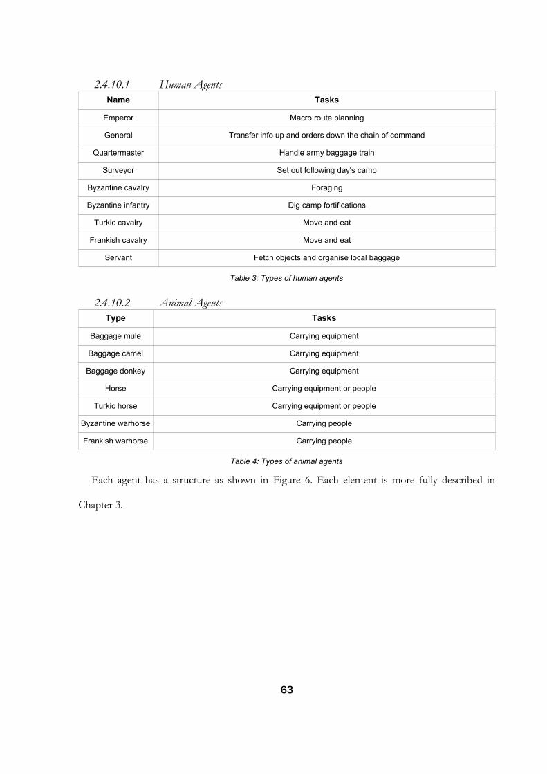
2.4.10.1 Human AgentsName Tasks

Emperor Macro route planning

General Transfer info up and orders down the chain of command

Quartermaster Handle army baggage train

Surveyor Set out following day's camp

Byzantine cavalry Foraging

Byzantine infantry Dig camp fortifications

Turkic cavalry Move and eat

Frankish cavalry Move and eat

Servant Fetch objects and organise local baggage

Table 3: Types of human agents

2.4.10.2 Animal AgentsType Tasks

Baggage mule Carrying equipment

Baggage camel Carrying equipment

Baggage donkey Carrying equipment

Horse Carrying equipment or people

Turkic horse Carrying equipment or people

Byzantine warhorse Carrying people

Frankish warhorse Carrying people

Table 4: Types of animal agents

Each agent has a structure as shown in Figure 6. Each element is more fully described in

Chapter 3.

63

2.4.11 Agent Architecture

2.4.11.1 InboxEach agent has an Inbox which operates like an email inbox. Any messages from other agents

are placed here where they wait until the agent can process them. They are then removed.

2.4.11.2 Plan QueueThe plan queue is the list of tasks that the agent has to fulfil. They are placed in the order in

which they will be processed. Processing tasks may result in more plans being added to the

queue.

2.4.11.3 Perception BaseThe perception base or context contains the information that the agent knows about the

world including information about the environment and other agents.

2.4.11.4 AttributesThe attributes of an agent specify those aspects of the agent that can change from agent to

agent. They can modify behaviours.

64

Figure 6: Agent architecture

2.4.11.5 BehavioursAn agent's behaviours are hard-coded into the model and govern the way the agent processes

messages and plans from its queue.

An agent will either receive a message or sense a situation in its perception base that requires a

response. It will then process the resulting plan from its plan queue that will trigger its internal

behaviours. The actions of these behaviours may be modified by the agent's attributes.

2.5 Human Agents: AttributesThe model is primarily concerned with the movement and provisioning of the Byzantine army

and the agent's attributes should be restricted to those we need to accomplish our objectives.

Some attributes are set during the model's initialisation and do not change while some vary

during the operation of the model. The use of each agent's attributes and the circumstances

under which they change are described in more detail in Chapter 3.

Attribute Variable Type

Notes

ObjectID Integer A unique agent identifying number

Unit# Integer A number identifying the unit to which the agent belongs

Weight Integer The agent's weight in kilogrammes

AdHocUnit# Integer Used to enable agents from different units to be formed into temporary units to perform certain tasks (foraging, ditch digging etc.)

VisionRange Integer The distance in metres that the agent can see unless interrupted by objects or terrain

MovementSpeed Double The maximum speed that the agent can move in each time step of the simulation

CarryingCapacity Integer The maximum load that the agent can carry for extended periods in kilogrammes

Superior Integer The ObjectID of the agent's superior in the army's chain of command

Table 5: Human attributes

65

2.6 Human Agents: Behaviours

2.6.1.1 HealthAn agent's primary responsibility is to its own survival. It will obey its own plan queue until its

health reaches a certain point, at which point the agent 'fails'. This will result in it dropping out

of the army's organisational structure. A similar process occurs when the agent's energy

expenditure exceeds its consumption. If this happens regularly over an extended period or

catastrophically in a short time then the agent will inform his superior but will continue normal

operation until his health is affected (Figure 7).

66

Figure 7: Agent health decision making

Generals have different health decision making as befits their higher status within the army.

This also applies to mercenaries, surveyors and quartermasters (Figure 8). As can be seen, higher

status members of the army will first turn to the army's baggage train and then other units'

supplies rather than starve. This ensures they will never be without food, the army will fail before

a general starves to death. Also note their response to fatigue, instead of merely reporting

themselves in need of a rest like common soldiers they will overestimate the need for their unit

to rest when messaging the Emperor. This will ensure they have a higher chance of getting a rest

day for the army. Naturally the general will rely on servants to do all the actual work in this

process.

67

2.6.1.2 EmperorThe Emperor is responsible for planning the overall route to Manzikert. He will decide which

settlements to pass through and on which days to move (Figure 9). The army will need at least

one day of rest per week regardless of condition otherwise the horses will develop health

problems. It is possible that the condition of the army will demand more rest than that at times,

especially after a period with insufficient rest or food.

68

Figure 8: General's health decision making process

The Emperor will already have the location of the next camp as the surveyors will have sent a

messenger back the previous day. The Emperor will have a daily status update from each General

regarding the units under their command. The generals will supply the emperor with a percentage

of units that have insufficient food and need rest. The emperor can then make his decisions on

this basis. The Emperor goes through this decision making process each morning. Each evening

he does nothing but consume food.

69

Figure 9: Emperor's decision making process for each day's march

2.6.1.3 GeneralGenerals have a different decision making process regarding their own well-being as described

above. They include members of the bureaucracy and their function in the ABM is primarily to

act as intermediaries between the combat units and the Emperor. In the Byzantine army their

tasks would have included liaising with mercenaries, making decisions regarding the discipline of

the army and dealing with organisational matters too trivial for the Emperor to be bothered with.

In the ABM however all decisions affecting the whole army are taken by the Emperor agent. This

represents a reality of consensus, meetings and slightly devolved power that is hard to model and

does not significantly affect the movement or supply factors of the army's march. Some of the

officer class will also have their commissions based on personal wealth or power and so this

strata of the army will have been padded with largely unnecessary roles anyway.

Each morning the generals immediately under the Emperor in the hierarchy will deliver

messages containing the army's status allowing the Emperor to decide whether the army moves,

rests or forages (see above). Beyond this and the passing of messages up and down the army's

structure they have no decision making processes. There will be Generals with unit numbers that

do not have a place in the army's hierarchy to represent members of the bureaucracy. This

ensures they use the General's health decision making process but play no other role in the army.

2.6.1.4 QuartermasterThe quartermaster's primary responsibility is to determine the ration rate of the army. The

ration rate is a percentage value that affects how much food an agent eats each day. 100%

represents the full value of calories needed to sustain a human during moderate activity. This can

be lowered as a response to dwindling stocks of supplies. There is a separate value for food and

water.

70

The quartermaster leads the army's baggage train and travels with it. Individuals from the

army can come and request food or water from the army's baggage train as their own units run

out. This will generally happen in camp. As the baggage train camps in the same part of the

camp each night then all agents will know where it is. Each morning the Quartermaster will go

through the process in Figure 10 and then message his servants to pass this message on to the

generals who will pass it down the chain of command. Thus the generals will know the ration

rate as well as having the info regarding troop energy and health from their subordinates.

2.6.1.5 SurveyorThe Surveyor is responsible for setting out the following day's camp. Like the Quartermaster,

the Surveyor is an agent representing the whole of the decision making apparatus of the

surveying team. In reality there would be a number of agents with specialised tasks related to the

71

Figure 10: Quartermaster's decision making process

planning and setting out of the camp. Within the ABM this is abstracted down to a surveying

agent who makes the decisions (Figure 11) and a series of servants who respond to his

commands. This simplifies the ABM architecture while still giving a reasonable number of agents

for movement and supply purposes.

The surveyor receives from the Emperor the location of the next waypoint, usually a

72

Figure 11: Surveyor's decision making process

settlement. The surveyor will plan a route to this location using the A* route planner. It will then

travel along this route with its team of servants. When it reaches the maximum distance that the

army can travel in a day it will assess whether this location is suitable for a camp. This will be

based on the availability of water and enough flattish ground to place the camp. If this place is

unsuitable the surveying team will travel back down the path looking for suitable locations. As

soon as it find one it will send a servant back to inform the Emperor where the camp is located

and then order the other servants to set out the camp. If it reaches the minimum march distance

without finding a suitable location it will return to the maximum move distance and declare that

the 'best worst' camping location and set up there.

The surveyor agent will have 2 variables no one else has, MaximumArmyMoveDistance and

PreviousArmyMoveDistance. The maximum distance is the furthest distance the army can move

during one day. If the army regularly manages to march this distance with plenty of time to set

up camp this will be increased. If it finds itself arriving at camp too late then it can be decreased.

The minimum march distance is 60% of this figure. The previous move distance is recorded

because the army will not always move its maximum distance due to the availability of decent

camp sites. Recording how far the army actually moved will avoid the increasing of the maximum

due to early arrival if the army only moved part of the maximum.

73

2.6.1.6 Byzantine CavalryThe Byzantine cavalry units will be primarily responsible for foraging if and when this is

required. Their increased speed and Greek language proficiency makes them more suited to this

role than infantry or mercenaries. An entire unit will be assigned to foraging, with the size to be

determined by the Emperor based on how much food or water is required. The leader of that

unit is designated the leader of the foraging party and his decision making process is detailed in

Figure 12.

74

Figure 12: Foraging leader's decision making process

2.6.1.7 Byzantine InfantryThe army's Byzantine infantry will be responsible for digging the ditch around the camp every

evening. Each unit of the infantry will be responsible for digging a particular stretch of ditch.

When a definite camp location is communicated back from the surveying team.

2.6.1.8 Turkic CavalryTurkic mercenaries will have two unique attributes: NumberOfHorses and CurrentHorse. Due

to the Turkic tendency to have many horses and to rotate which horse they ride in order to

spread the load each Turkic mercenary will keep track of which horse they were riding each day

and each morning.

2.6.1.9 Frankish CavalryFrankish mercenaries will tend to have a warhorse and another horse or two for riding. The

warhorse will be bigger and not carry equipment. The other horse(s) will be of regular size and

will be rotated between being ridden and carrying equipment if possible.

2.6.1.10 ServantThe servant is ubiquitous in the ABM, primarily because many tasks are aggregated into just a

few agents. Everyone with no definite function will either be a General or Servant depending on

their status. Servants will have a superior and will follow their superior until given an order by

them. They will also follow the soldier's health decision making cycle as detailed above.

2.7 MovementCentral to the MWGrid ABM is the movement model. The movement of the army as a whole

depends on the movement of each individual so if this movement is unrealistic, the output of

the ABM will suffer. Agent-based modelling is a computer-based simulation technique that has

already been used to simulate the movement of large groups of individuals, from Craig Reynolds'

work on flocking behaviours (Reynolds 1987) through to work in safety science and sociology

75

(Lansing 2002; Thompson and Marchant 1995). There are also a number of archaeological ABM

projects from the small and abstract (E. A. Smith and Choi 2007) to the large and

multidisciplinary (Kohler et al. 2008). Its architecture of autonomous software entities behave

according to their own internal rules and inhabit a landscape that can act as a source of resources

and a constraining factor to movement and is ideal for examining military organisation and

supply.

Creating an ABM involving tens of thousands of agents moving across a distance of over 700

miles presents many challenges, both technical and historical. Due to the incomplete nature of

the historical record there is no single source for agent organisation, behaviours or attributes. The

environment around which each will move is also based on incomplete and inadequate data. All

historical ABMs share similar problems but by modelling various hypothetical scenarios and

noting where and how they differ we can rule out the more impractical scenarios and establish a

set of parameters within which we can re-evaluate the historical record.

Modern agent-based models are widely used in the simulation of crowd movement

(Thalmann and Musse 2007) and this is an important part of this research into Byzantine army

logistics. How the many members of the army are organised while on the march affects the

speed of the army as a whole, which in turn affects consumption of resources and the

subsequent impact on the communities providing those resources. Efficient movement was

acknowledged by Byzantine military writers as being essential to the success of a military

expedition (Dennis 2001, 20; Dennis 1985). Unfortunately there are few sources regarding the

organisation involved and the procedures followed, contemporary histories being more

concerned with the battles and personalities of the time. It is this subject's very mundaneness

that results in a lack of adequate descriptions of the daily routine of an army on the march and

76

no detailed analysis of how this affected the territories passed through.

There are two types of movement required by the MWGrid ABM: macro-scale and micro-

scale. The macro-scale movement deals with the movement of the army as a whole. Although

one of the goals of the ABM is to examine how the movements of individuals translate into the

overall movement of the army, the movement of the army does not occur like a swarm of ants

relentlessly covering Anatolia until they reach their destination. As described above, some

element of control over the daily movement of the army is required. The intention must be to

have the whole of the army arrive at the following day's camp in plenty of time to set up their

tents and feed themselves. The army must also move in such a way as to be able to pick up

sufficient supplies in order to feed itself. For this reason an overall route plan will have been

made in advance so that the communities through which the army passes will have had the

opportunity to stockpile the required resources (Haldon 1999, 182). This overall route may have

been so specifically detailed as to include individual roads to be taken and settlements to be

visited down to very small villages or it may have operated on the regional level, specifying no

more than the regional centres at which supplies should be collected. For this reason, the ability

for the macro route to be determined during the run of the simulation is important. It can be

used to create a complete route from scratch using various hypothetical models or it can be used

to alter or provide fine detail to a route already specified in advance. All route planning is based

on the A* route planning algorithm, the technical details of which will be covered in Chapter 3.

2.7.1 Macro-Scale MovementMacro-scale route planning operates over the course of more than a day and determines the

overall route of the army. It specifies a series of waypoints through which the army will attempt

to travel. This can either be set in advance or be determined by environmental factors such as

77

access to food and water or in order to take advantage of major roads. It simulates the route

planning usually done in advance by the Emperor and whoever constructs the overall plan for the

campaign. The A* planning algorithm allows us to assign costs to various types of moves so that

if, for example, we assign lower costs to moves which pass through large settlements the macro

route will tend to go through large settlements. In this way many different considerations can be

modelled in order to examine their effect on route planning.

2.7.2 Micro-Scale MovementMicro-scale movement is something that happens at the level of the individual and is done by

all agents looking to move from one location to another. At this level the majority of agents will

just be following the macro route chosen in advance by the Emperor but still need to move from

location to location avoiding other agents. As crowding is an important mechanism in the overall

movement of the army, this must be simulated in some way. As there cannot be an infinite

number of agents inhabiting the same space, the model compares the size of each environment

cell with the sizes of all the agents within it to see if there is space for an agent to move into the

cell. If there is not, the agent's route planner will attempt to get to its destination while avoiding

cells with insufficient space.

2.7.3 Intermediate-Scale MovementDue to the massive difference in scale between the macro route plans and the micro route

plans, there is a need for an intermediate layer at which the officers of squads move from terrain

data point to terrain data point (see Figure 13). This is done to improve accuracy and

performance and is detailed in Chapter 3.

78

2.8 Calorie ExpenditureBeing able to determine the calorie expenditure of each agent has obvious modelling benefits.

Previous work such as Pryor and Engels have assumed a static figure for food requirements per

person per day. The resolution of the MWGrid ABM allows a more accurate calculation of the

energy expended for each agent. Not all activity by every agent will be modelled but the coarse

estimates produced by the MWGrid ABM can still be much more finely nuanced that the top

down approaches tried previously. As the ABM is able to record the location and activity of every

agent throughout the run of the simulation, conventional equations from exercise and sports

science can be used to calculate how many calories an agent uses in any given situation. The

following scheme is taken from the American College of Sports Medicine's Guidelines for

Exercise Testing and Prescription (Balado 1995, 276).

In order to calculate the calories expended while walking, we first need to calculate the volume

of Oxygen consumed (VO2). This can then be used to calculate the calories burnt compared to

the amount of carbohydrates and fat consumed.

VO2 = R + H + V

R = 3.5ml per kg per minute

H = 0.1 x walking speed (in m/min)

79

Figure 13: The three levels of route planning

V = 1.8 x speed (in m/min) x grade (as a decimal)

There are acknowledged flaws in this equation but these relate to people under the age of 18

and for walking on the level. By assuming all the members of the army are aged 18 and over the

first of these situations is avoided. As each agent will not be walking on the level for very long

due to the undulating nature of the Anatolian terrain any inaccuracy derived from this should be

minimal.

For example, an agent walks for an hour at 3mph up a slope of grade 0.05, or 1 metre up for

every 20 metres across. This would give us:

3.5 + 8.047 + 7.2423 = 18.7893 ml per kg per minute

This first value is in ml of O2 per kg of body weight (plus any weight carried) per minute. This

provides a good value against which to calibrate our data as values of over 50 can only be

accomplished by a fit individual and values of 80+ are probably unreasonable for anyone likely to

be in the Byzantine army. If this result is multiplied by a plausible weight for an individual plus

clothing, 70kg, we get:

18.7893 x 70 = 1315.251 ml per min or 1.315251 litres per minute

Any carried weight would be added onto the weight of the individual, allowing a calculation

of how energy expenditure is affected by increased load. Using Table 13 of Carpenter's Tables,

Factors and Formulas for Computing Respiratory Exchange and Biological Transformations of

Energy (2010) we can find a figure which, when multiplied with our result for litres of O2 per

minute, will give us the value of kilocalories burnt per minute. The multiplier depends on the

amount of carbohydrate or fat consumed as they are transformed into energy differently. For this

example we will assume 100% carbohydrate consumption, this gives us a figure of:

80

1.315251 x 5.047 = 6.638071797 kcals per min

In our example of an agent walking for an hour they would burn about 398.28 kilocalories per

minute.

Several points can be noted from these calculations. There are standard ways of calculating

calorie expenditure that can easily be calculated by the MWGrid ABM. These can give a coarse

indication of the amount of energy expended by each agent which will in turn relate to the

amount of food required. This could be affected by how much equipment or supplies each agent

was being asked to carry. There is also a feedback between the types of food eaten and the

amount of calories required. Although the differences aren't extreme, around a 7% difference

between 100% carbohydrates and 100% fat, they make become significant when multiplied by the

number of agents and over the length of the campaign.

Not all of our agents are infantry so the ability to determine the energy expenditure of riding

a horse would be essential in order to calculate energy expenditure for the whole army. A small

study was carried out by Devienne and Guezennec (2000) in which oxygen consumption was

measured for 5 different riders and 4 different horses during dressage. Oxygen consumption

varied depending on the person and on the type of movement, as seen in Table 6.

Rider Walk - VO2 (litres per minute)

Trot - VO2 (litres per minute)

1 1 1.85

2 0.56 1.4

3 0.72 1.55

4 0.6 1.17

5 0.64 1.43

Mean 0.7 1.48

Table 6: Oxygen consumption of horse riders (after Devienne and Guezennec 2000)

These values are in litres per minute and already have the weight of the rider taken into

81

account. The only further calculation that would need to be performed is multiplication by the

modifier from Carpenter. The above only allows a coarse measurement of calories expended

however if we assume all other activities remain the same we can estimate the difference between

different types of activity and how this relates to supply consumption. This in turn allows us to

coarsely estimate the effects on the settlements on whom the supply burden fell.

2.9 The Environment

2.9.1 What Was the Environment Like?The environment of the MWGrid ABM is the environment of Byzantine Anatolia. Not all of

Anatolia needs to be modelled as there are only a certain number of viable routes between

Nicomedia and Manzikert. The environment needs to be large enough to encompass all the

viable routes but with as little extra detail as possible in order to minimise data storage. Each

aspect of the environment is treated separately due to the differing resolutions and data formats

of the source data. Each aspect of the environment is detailed below.

The environment consists of two elements.

• Environment slices

• Weather data

An agent-based model (ABM) consist of two main elements; autonomous agents and the

environment they move around in and interact with. In the MWGrid ABM the environment

represents Byzantine Anatolia in AD 1071. The ABM environment is split up into slices with

each aspect of the environment occupying a separate slice. This assists the organisation and

storage of the environment.

The environment slices are brought together in ArcGIS and GRASS (using QuantumGIS as a

82

front end) and output as ESRI ASCII text files. This is necessary because the data sources are of

insufficient resolution and in inappropriate formats to be simply imported into the ABM as is.

Continuous data such as terrain can be read directly into the ABM as ESRI ASCII files in either

5m2, 50m2 or 500m2 resolutions. Sparse data sets must be written to ESRI ASCII files first but

can then be converted into a simple list of locations that occupies much less disk space.

The area covered by the environment lies between 38° - 42°N and 28° - 44°E (Figure 14). The

resolution of the data varies depending on the slice. The ABM uses a resolution of

0.0000449944° N-S and 0.0000570004° E-W giving a cell size of roughly 5m x 5m. This was

chosen as it represents the smallest reasonable gap size that troops will have to travel through. If

this resolution were used for the environment slices each would need a standard ESRI ASCII

raster file of 24,954,230,000 cells (280,700 x 88,900). This would create an unusably large single

ESRI ASCII file, requiring around 140Gb of disk space for a single slice. It is also much finer

than the resolution of the base data, the finest resolution data we have is the ASTER terrain data

at roughly 50mx50m.

Initially, the ASTER data was intended to be interpolated to the 5mx5m resolution however

standard methods of interpolation cannot introduce the kind of fine grained detail needed to

represent the narrow defiles and awkward terrain originally intended to be modelled. Fortunately

the movement of the army in highly restricted circumstances will be modelled in circumstances

such as the exit from the daily camp and the crossing of the Halys. For these circumstances a

5mx5m terrain resolution is unnecessary. This also means the ASCII files containing the

environmental data are more practically sized.

When the ASCII data is loaded into the ABM it will be fitted into the model's 5mx5m grid. In

the case of raster data such as the ASTER and Globcover terrain data, each cell of data from the

83

ASCII file will be expanded over 10 or 100 ABM cells depending on the resolution. In the case

of settlement vector point data, the settlement will be placed in the centre of the block of 100

cells. Road vector data will be converted into an ASCII raster grid and imported in the same way

as settlement point data. The ABM will then create road links between the points at the

appropriate width.

Size label N-S resolution (degrees)

E-W resolution (degrees)

Rows Columns Approx cell size

Approx file size

LOW – low 0.00449944 0.00570004 889 2807 500m2 14Mb

MED - medium 0.000449994 0.000570004 8889 28070 50m2 1Gb

FUL – full ABM 0.0000449944 0.0000570004 88900 280700 5m2 50Gb

Table 7: The different sizes of environmental slice

No environmental slices use full ABM resolution as this is unnecessary and creates files of

unwieldy size, it is purely used inside the ABM. Medium resolution is used for data that is

supplied in a similar resolution such as the ASTER terrain data or for features of small size such

as roads. Low resolution is used for features of large size such as settlements of for data where

higher resolution is not needed such as the Globcover land use data.

84

2.9.2 Environmental Slices

2.9.2.1 Height – A Digital Elevation Model of Anatolia.

2.9.2.1.1 ResolutionMedium

2.9.2.1.2 SourceThe height data is derived from ASTER GDEM data. The ASTER GDEM (Advanced

Spaceborne Thermal Emission and Reflection Radiometer Global Digital Elevation Model) is a

joint operation between NASA and Japan's Ministry of Economy, Trade and Industry (METI)

and was released for public use on 29th June 2009 (Tachikawa et al. 2011). It was created by

compiling 1.3 million visible and near-infrared (VNIR) images taken by the ASTER satellite using

single-pass stereoscopic correlation techniques, with terrain elevation measurements taken

globally at 30 meter intervals. Using modern height data is justified as the terrain of Anatolia,

while part of a geologically active region, is not significantly different to that of the 11th century.

85

Figure 14: Anatolia with the MWGrid environment boundary in red

As the file containing this data is approximately 1.4Gb it has been zipped and is separated into

partitions that are only loaded when required.

2.9.2.1.3 FormatInteger. Height above sea level in metres

2.9.2.1.4 EffectHeight affects route planning and is used with weather to calculate how many calories are

burned during movement. It is also used with Transport and Terrain to affect movement speeds.

2.9.2.2 Settlement – Indicates Location and Type of Settlement.

2.9.2.2.1 ResolutionLow

86

Figure 15: ASTER GDEM data for Anatolia

2.9.2.2.2 SourceThe settlement data is digitised from the Tabula Imperii Byzantini (TIB) maps (e.g. Koder and

Hild 1976; Belke and Mersich 1990; Hild and Hellenkemper 1990), inserted from ancient sources

and extrapolated from known data. The Tabula Imperii Byzantini maps are part of an attempt by

the Austrian Academy of Sciences to map the geography of the Byzantine Empire. The results

have been published since 1976 in geographically separate sections and rely on historical records,

archaeological evidence, toponyms and the physical state of the landscape (St Popović 2009).

2.9.2.2.3 FormatLocation, name and type of settlement. The settlement types are taken from the TIB maps as

described in Table 8.

87

Figure 16: Settlements from all sources

GIS layer Subcategories Description

Walled settlements Seat of archbishopSeat of bishop

None

Cities with defensive walls, subdivided according to ecclesiastical status

Citadel settlements Seat of archbishopSeat of bishop

None

Cities with no extensive defensive walls but with an acropolis or citadel, subdivided according to ecclesiastical status

Unfortified settlements Seat of archbishopSeat of bishop

None

Cities with no significant defensive feature, subdivided according to ecclesiastical status

Table 8: Settlement types

Only the walled cities are named, other sites are recorded by position and subcategory only.

Due to the difficulties of incorporating the TIB maps into the co-ordinate system of GIS, the

areas of overlap do not precisely correspond. This resulted in minimal distortion of the

settlement data. Locations of the settlements that appeared on two maps were captured

somewhere between the locations indicated on each digitised map.

As the TIB data does not cover the whole of the area simulated in the ABM, some method of

extrapolating the data from the TIB across the whole area was needed. As modern settlement

location data was available, this was used to generate the extra settlements required. To this end,

the area was split into 3 different areas; the area covered by the TIB maps, the area of Anatolia

west of this and the area to the east (Figure 17).

88

By analysing the data from the area covered by the TIB we can examine the proportions of

each type of settlement and use these same proportions to add detail to the settlements of the

extrapolated areas. We can also compare modern settlement densities in each of the three areas

to give a more plausible density in the simulated environment. Modern Anatolia is more densely

settled towards the west than the east, a pattern likely to be reflected in the Byzantine era,

especially considering the Seljuk raids of the 1050s onwards (Attaleiates 1853, 148). For this

reason the fact that the modern data finishes approximately 50km west of the edge of the

simulated area is not factored into the calculations, depopulation due to Seljuk raids would have

made up for any inaccuracy this introduces. Obviously the presence of a modern settlement

should not imply the presence of one in the Byzantine era but using modern data should at least

reflect general areas of high population density and ensure settlements are not placed in lakes or

in impassable terrain. The modern data is also considerably more complete than the TIB data,

89

Figure 17: The area covered by the TIB maps with the West and East areas of extrapolated data

which partially reflects patterns of archaeological research as well as patterns of settlement.

The process of creating the data consisted of five phases:

• Digitising the TIB data (Figure 18)

• Importing the modern data (Figure 19)

• Determining the modern settlement density (Table 9)

• Extrapolating settlements in the West and East areas based on the TIB data (Table 10)

• Random selection of modern points to generate an appropriate settlement density and

composition in the West and East areas (Figure 20)

90

Figure 18: Settlement data derived from TIB maps

Area Name Area (km2) # of modern settlements km2/settlements

West 45520 166 274

TIB 242152 649 373

East 228340 386 592

Table 9: Modern settlement density in the three areas

91

Figure 19: Modern settlement data

Type of settlement # in TIB area extrapolated # in WestTIB * 166 / 649

extrapolated # in EastTIB * 386 / 649

Walled city - archbishopric 16 4 10

Walled city - bishopric 22 6 13

Walled city - other 7 2 4

Citadel city - archbishopric 3 1 2

Citadel city - bishopric 16 4 10

Citadel city - other 46 12 27

Unfortified settlement - archbishopric 2 1 1

Unfortified settlement - bishopric 53 14 32

Unfortified settlement - other 210 54 125

Total 375 98 224

Table 10: Extrapolation of settlement numbers and types

As can be seen, the number of settlements recorded in the TIB is just over half that of the

number of modern settlements. Obviously not all settlements are recorded so the number of

92

Figure 20: Modern settlements split into TIB categories. Orange dots are discarded points

settlements in the Byzantine era would likely be closer to that in the modern era, taking into

account the opposing modifiers of greater modern population and lower Byzantine urbanism.

Despite this, the majority of small rural settlement would have been too small and/or poor to

have enough supplies to significantly affect the provisioning of the army, their surplus having

been already transported to the nearest main settlement anyway. For this reason the model keeps

the settlement density recorded in the TIB maps and removes unwanted settlements at random.

2.9.2.2.4 EffectEach category of site cab be assigned a number of inhabitants representing the population of

the settlement and it's immediate hinterland (Table 11). These were derived from 16th century

data (Dagron 2002, 394) however historical demography can be imprecise at the best of times

and these figures are intended only as a guide. The number of inhabitants will be used in

conjunction with the ESA Globcover data to produce two values for each resource, a total

amount and a surplus amount. The total amount is the amount in that settlement for use by the

inhabitants in addition to the surplus. The surplus is the amount over and above what the

inhabitants need to survive. The surplus amount is the amount normally available to the army,

however in times of shortage the army may force the settlement to hand over any extra, up to the

total. It should be noted that the values for settlement size and the accompanying amounts of

supplies represent a highly speculative hypothetical model. The MWGrid ABM can be used as a

tool to provide some kind of framing evidence for these figures, possibly indicating the practical

limits of food surplus.

93

TIB category Assumed population size

Walled settlement (archbishopric) 30000

Walled settlement (bishopric) 15000

Walled settlement (no bishop) 10000

Citadel settlement (archbishopric) 10000

Citadel settlement (bishopric) 5000

Citadel settlement (no bishop) 4000

Unfortified settlement (archbishopric) 4000

Unfortified settlement (bishopric) 3000

Unfortified settlement (no bishop) 2000

Table 11: Assumed population size for each TIB category

2.9.2.3 Globcover – The European Space Agency's Vegetation Cover Database.

2.9.2.3.1 ResolutionLow

2.9.2.3.2 SourceThe ESA's Globcover 2009 land cover map (http://ionia1.esrin.esa.int/). Due to the

difficulties in recreating the ecology of the whole of the ABM study area, modern land use data

is used. This obviously creates inaccuracy as changes in agricultural technology and settlement

patterns will result in different land uses. The GlobCover categories have been used as the basis

for coarsely derived values for food, fodder and firewood as an indication of resources available.

94

2.9.2.3.3 FormatAn integer indicating the type of agricultural terrain of an area.

2.9.2.3.4 EffectThe Globcover categories are used to determine the amount of animal fodder, food from

arable agriculture and firewood that are available to each settlement (Table 12). These values are

estimated on a scale of 0 – 3. The ABM can perform a range query on all land within a certain

radius of a settlement in order to determine how much of each resource the settlement has

available to it. This can also be performed by the army in rural areas to determine how much

firewood or fodder can be foraged.

95

Figure 21: ESA Globcover data

Globcover type

Description Fodder amount

Food production

Firewood amount

11 Post-flooding or irrigated croplands (or aquatic) 1 3 0

14 Rainfed croplands 1 3 1

20 Mosaic cropland (50-70%) / vegetation (grassland/shrubland/forest) (20-50%)

3 2 2

30 Mosaic vegetation (grassland/shrubland/forest) (50-70%) / cropland (20-50%)

3 2 3

40 Closed to open (>15%) broadleaved evergreen or semi-deciduous forest (>5m)

1 1 2

50 Closed (>40%) broadleaved deciduous forest (>5m) 1 1 3

60 Open (15-40%) broadleaved deciduous forest/woodland (>5m)

2 2 2

70 Closed (>40%) needle leaved evergreen forest (>5m)

1 1 3

90 Open (15-40%) needle leaved deciduous or evergreen forest (>5m)

2 2 2

100 Closed to open (>15%) mixed broadleaved and needle leaved forest (>5m)

1 1 2

110 Mosaic forest or shrubland (50-70%) / grassland (20-50%)

3 1 3

120 Mosaic grassland (50-70%) / forest or shrubland (20-50%)

3 2 2

130 Closed to open (>15%) (broadleaved or needle leaved, evergreen or deciduous) shrubland (<5m)

1 1 2

140 Closed to open (>15%) herbaceous vegetation (grassland, savannas or lichens/mosses)

3 2 1

150 Sparse (<15%) vegetation 0 0 1

160 Closed to open (>15%) broadleaved forest regularly flooded (semi-permanently or temporarily) - Fresh or

brackish water

1 1 2

170 Closed (>40%) broadleaved forest or shrubland permanently flooded - Saline or brackish water

0 1 3

180 Closed to open (>15%) grassland or woody vegetation on regularly flooded or waterlogged soil -

Fresh, brackish or saline water

1 2 1

190 Artificial surfaces and associated areas (Urban areas >50%)

0 0 0

96

200 Bare areas 0 0 0

210 Water bodies 0 0 0

220 Permanent snow and ice 0 0 0

230 No data (burnt areas, clouds) 0 0 0

Table 12: Globcover categories with associated resource values

2.9.2.4 Transport – Presence of Roads

2.9.2.4.1 ResolutionMedium

2.9.2.4.2 SourceDigitised from the Tabula Imperii Byzantini maps, inserted from ancient sources and

extrapolated from known data.

A similar process was followed with the road data as for the settlement data. Unfortunately

97

Figure 22: The roads represented in the ABM

roads are less amenable to the approach followed with settlements as, unlike settlements which

can look plausible when randomly selected, roads have a pattern to their path. They usually start

somewhere and end somewhere and, in between, follow a reasonable path. With this being the

case a much more minimal approach was taken to expanding the data outside the area covered by

the TIB maps. Only roads between major settlements (walled settlements with archbishoprics)

were added. The routes themselves were taken from whichever modern routes most aligned with

the routes from John Haldon's 1999 map (Figure 23).

Within the area covered by the TIB maps, roads were more difficult to align between different

maps than settlement data. In these cases the roads were tidied up as much as possible, the new

roads being created in between where the TIB maps indicate them. On some occasions there

were roads marked on some maps that weren't present on others. As a result some roads do not

98

Figure 23: Map of Anatolia from Haldon (1999)

appear to go anywhere. Ultimately there are no easy answers to this problem. The roads

themselves are only approximate not having been proofed along their whole length. Dating roads

is also notoriously difficult (French 1981) so some roads present in the TIB maps may not have

been in use in AD1071.

2.9.2.4.3 FormatEach pixel contains either 0 (no road present) or 1 (road present)

2.9.2.4.4 EffectRoads are primary factors in macro route planning for the whole army. Where a route exists

which follows a major road it will be taken due to its positive effects on movement speed and

army coherence. It also affects movement, with agents travelling faster on roads and following

them whenever practical.

2.9.2.5 Water – Presence and Type of Water

2.9.2.5.1 Sourcehttp://www.diva-gis.org/gdata

2.9.2.5.2 FormatAn integer identifying the type of water (Table 13).

2.9.2.5.3 EffectActs as a water source for humans and animals. Acts as a barrier to movement.

99

Data type Type of water

0 Land subject to inundation

1 Lake

2 Intermittent streams

3 Perennial streams or rivers

Table 13: Water data types

2.9.3 Weather DataThe climate of Anatolia in the late 11th century was not significantly different to that of

recent years (England et al. 2008). This being the case, modern data can be used to provide

hypothetical weather schemes for Byzantine Anatolia that can affect movement and the amount

of water and food consumed.

Three years will be selected from the data available, one year much hotter than average, one

much cooler and one as close to average as possible. These three different sets of data, one hot,

100

Figure 24: Water data

one average and one cool, can be used to assess the effects of weather on energy and water

consumption of the agents.

Hourly temperature data will be extrapolated from the daily maximum and minimums by

using a typical curve of temperature change throughout the day. This will produce an hourly

temperature for each weather station in each of the three sample years. When an agent needs to

determine the temperature of the location he is at the ABM can perform a simple calculation to

extrapolate a temperature from the 3 nearest weather stations.

Weather data is available via the internet (http://climexp.knmi.nl), however daily coverage of

Anatolia is relatively sparse. The following weather stations were found to have sufficient daily

data to be useful.

• Istanbul

• Rize

• Kastamonu

• Sivas

• Gumri

• Van

101

The only data common to all stations that were substantially complete were between 1957 and

1992. In order to narrow down the amount of data so that a hot, cold and average year could be

chosen, only data from 1980 - 1992 inclusive were used. As not all stations had the same hottest

year, coolest year or average year a system was introduced whereby the years were ranked by

average mean temperature. The hottest two years were separated for each station, along with the

coolest two years and the median year. From this, the hottest year was chosen as 1989, the coolest

as 1992 and the average year was 1984 as it was the median year twice and never appeared in

either the hottest or coolest years for any weather station.

Now that these years are selected, the daily maximum and minimum temperatures can be

downloaded and applied to a standard temperature curve over the course of the day. Whenever

an agent requires the temperature at its current location it can request the temperature from each

of the three nearest weather stations and average them, weighted by distance.

2.10 ConclusionJust as there were a variety of levels on which campaign organisation worked in the Byzantine

102

Figure 25: Location of weather station with the ABM area

army so there are a variety of levels on which this simulation is modelled. The macro decisions

regarding the overall route can be either pre-scripted or based on criteria built into the route

planning network. This creates waypoints that are navigated between using the grid-based A*

route planner. The route is then subdivided based on the length of the daily march and a series

of camps specified. These can be altered at the end of each day based on the experiences of the

previous day's march. Each day the army makes and breaks camp according to a set routine.

The ABM design detailed here is constrained by three main factors; the types of data available

in a suitable format, the behaviours that can be plausibly modelled and the aspects of the

Byzantine army and the Anatolian landscape that are necessary to produce the output required.

As in most archaeological contexts, the data required is incomplete, unreliable and varies in

spatial and temporal resolution. These problems are not insurmountable however. Where data is

absent, plausible hypotheses can be introduced. Where multiple plausible hypotheses exist and

the choice makes an appreciable difference to the output then multiple hypotheses can be

modelled. Historical data can be used not only to create the model but also to calibrate the

results. The following chapter describes the implementation of the model, including how it was

developed and the choices made regarding which factors were important enough to ensure the

output was useful.

The result of the technical efforts will be an agent-based model that incorporates the terrain

and weather of Anatolia with hypothetical supply levels and distribution into an environment

over which our agents can travel. By creating and running a series of 'what if ?' scenarios with

armies of different sizes and compositions travelling in a landscape with different levels of

supply and water availability. The results of these scenarios will allow us to draw conclusions

about how armies behave in ideal circumstances. We can then compare this with the historical

103

record and attempt to explain any differences.

Finally, whilst appreciating that all models are wrong (Box and Draper 1987, 424), the project

attempts to make a break with traditional historic analysis in the manner in which it incorporates

individual action within an interpretative framework that can add to our understanding of a

historic event or process. While small glimpses into individual behaviours can be found in the

work of Attaleiates and modern research tools such as the online Prosopography of the

Byzantine World (http://www.pbw.kcl.ac.uk), these do not allow us to examine the interactions

common in complex systems. With the emergent behaviour modelled in the ABM the project

seeks to add new evidence to existing debates about the movement of large numbers of troops

across a pre-industrial landscape. We can examine the relationship between human and animal

stamina, unit organisation and how this impacts on army speed in ways previously unavailable. To

the movement model will be added modelling of the use and transport of food and supplies.

Levels of supplies can be varied to investigate the impact on the army as a whole. With its

modular nature, Agent-based Modelling can test different hypotheses regarding agricultural

productivity and settlement by ensuring that the route planning decision making remains constant

while varying the resource levels. The differences this creates between otherwise identical runs of

the model can help inform our interpretations of how Byzantine military operations were

planned and executed.

104

3 Implementation

3.1 IntroductionOnce the model has been designed, implementation can begin. The scale of the project and

the process of development require multiple models to be created. This enables features to be

added sequentially and tested individually while still using the model to create useful data. Some

aspects of the ABM require others to be complete beforehand and some do not. For instance,

when dealing with crowding and movement it is unnecessary to include energy expenditure data.

In contrast, when examining energy expenditure the crowding and movement mechanisms must

be in place as these will affect the number of calories burned. For this reason a basic model was

created which focussed on the movement aspects of the army and then subsequently changed

and expanded in order to focus on such areas as army composition, size and calorie expenditure

during the Manzikert campaign.

In this chapter I will detail the process of translating the design described in the previous

chapter into a series of functioning agent-based models. I will describe the technical details of

how it was implemented and explain how and why the models deviate from the design as so far

described. I will explain the limitations of the software and how these are affected by the

hardware that was made available. Any technical terms will be explained in the glossary.

3.2 Temporal and Spatial ResolutionThe micro-scale movement described in the previous chapter is essential in our model of the

movement of the Byzantine army. It is this level that is accessible to agent-based modelling yet is

below the level of the work of Pryor and Engels' attempts to look at the movement of the

Crusaders and Macedonians respectively (Pryor 2006; Engels 1978). If we are to add the

complexity possible with ABM to these techniques we must be able to simulate the phenomena

105

that would make the movement of the army as a whole more than just the sum of the speed and

size of its individual elements. For this reason, the resolution of the model needs to be

appropriate to simulate phenomena such as crowding and the concertina effect, emergent

behaviours from individual movements. In order to achieve the granularity required to plausibly

simulate these behaviours the ABM uses one agent to represent one member of the Byzantine

army. This will increase the processing time of the model as the number of agents will be greater

than if each agent represented a unit but it is in the interactions between these agents that the

overall movement of the army will come from. Sacrificing resolution at this level will

compromise the plausibility of the model.

This 1:1 ratio extends to the human members of the army but not the animals. On the march

cavalry horses will either be ridden or, in the case of spare horses tethered to their owner's mount

so there is no need to separately model horses. The baggage train and baggage handling

procedures for individual squads is not modelled but they will be taken into account in the

concluding chapter.

3.3 Building the ModelThe MWGrid ABM is written in Java. Java is an object-oriented programming language and is

well suited for the creation of agent-based models (Gilbert and Troitzsch 2005, 22). It is relatively

easy to learn, powerful and most importantly it is portable, it can be run on many types of

computer architecture with no change in the code (Gosling 2000). This ability to be written once

then recompiled to run on various systems was seen as an important characteristic given the

project's initial aim to run the model in a distributed environment. It allowed the project to be

flexible regarding which distributed computer cluster that the model would run on while still

allowing it to be run on desktop machines for development and debugging.

106

As multiple individuals needed access to the code of both the models and the distributed

infrastructure being developed to run them, the ABM was stored on an SVN repository on the

servers of the University of Birmingham's Computer Science department. This ensured that the

software could be accessed from anywhere with an internet connection and enabled some

measure of version control to be exercised. This meant that two programmers could not change

the same section of code at the same time without an explicit resolution of any problems caused.

Eclipse was used as a development environment due to its easy integration with Java, its ability to

seamlessly work with SVN repositories, its industry standard nature and the fact that, being open

source, it was free.

3.3.1 Focussing on the Micro-ScaleDue to the scale of the model as it was designed, a distributed agent-based model

infrastructure, PDES-MAS, was developed by the MWGrid project members from the Computer

Science department of the University of Birmingham. This consisted of the software required to

run the model on multiple machines at once, vastly increasing the computing resources available

to the model. As PDES-MAS was written in C++, an intermediate layer of software, the

middleware, was created to provide an API that the model could use (Figure 26). This was

necessary to convert the Java software calls into instructions the C++ code could handle as well

as providing helpful classes for the model and constraining its behaviour to avoid actions that the

PDES-MAS software would not be able to handle.

Due to the experimental nature of the infrastructure (Lees et al. 2005) and the departure of

the original Computer Science Research Fellow, the infrastructure was not completed in time to

be used in this research. As the model was being developed to use the API of the middleware

operating between the ABM and the distributed infrastructure the need to abandon the

107

distributed element of the ABM caused some rewriting. As some of the functionality of the

middleware provided classes that were useful to the ABM these were kept in. This included the

Location class, the Message class and the Value class used to extract values from Environmental

slices. The basic handling of environment slices, the first Python script to produce Blender

animations and the basic core of the A* route planner were also developed by the MWGrid

Computer Science Research Fellows, Bart Craenen and Rob Minson. All other software used in

this project including all the rest of the ABM, the second Blender Python script and the file

processing tools in both Java and OpenOffice Calc were written by Philip Murgatroyd. The Java

ABM consists of nearly 6500 lines of code.

As the distributed software infrastructure was a parallel development, to be described in

future work, a separate version of the ABM was required to run on a single PC-compatible

computer. The reduction in computing power meant either the scale or the resolution of the

model would have to be reduced. This resulted in the decision to reduce the scale of the model

and focus on the effects of a day's march. A day's march is a discrete unit of time on a military

108

Figure 26: The intended MWGrid infrastructure (from Murgatroyd et al. 2011)

campaign, especially in the pre-industrial era. The lack of artificial lighting in addition to security

issues meant that the aim was to have all troops in the camp before sunset, preferably with

enough time to set up camp and make food. By modelling a day's march it is still possible to

examine the effects of crowding on the overall speed of the army. Individual elements such as

the speed and composition of the army can still be varied to determine their effects on overall

speed. In order to examine macro-scale movement a series of day's marches can be run over

different terrain in different conditions. Nine different sets of scenarios have been run with a

different version of the MWGrid ABM in each case. The scenarios are run with a specific goal in

mind and as such, different models are required to best reach that goal. The basic functionality of

the whole system including the ABM, the input files, the output files and the intermediate

processing steps is detailed in this chapter. The specific modifications carried out for each of the

nine sets of scenarios are detailed in Chapter 4, along with the results and analysis.

3.4 The Simulation ProcessWhen running a simulation, a series of steps are followed (Figure 27). The ABM takes the

parameters of its scenario from an initialisation file. This file specifies the size and composition

of the army, the starting and finishing points of the army's march, the route planning and

flocking parameters, the camp layout and the speed of the cavalry in various modes. This file is

loaded by the ABM in order to set its parameters. Having these parameters in a text file ensures

that the Java code does not need to be recompiled if changes are needed to the scenario. The

MWGrid ABM sets up a scenario based on the contents of the initialisation file and processes

the simulation over a sequence of consecutive timesteps known as 'ticks'. These ticks represent a

set period of real world time, within the MWGrid ABM this is usually about 3.7 seconds, as

explained on page 151. The ABM outputs two files: the tickfile which records the location and

109

status of each agent on every tick of the simulation and the dayfile that records aggregated data

about the whole day's march for each agent. Each of these files are used to access different types

of data. In order to process this data, the tickfile is processed by a Python script in Blender to

produce animations and the dayfile is loaded into an OpenOffice Calc template to produce

statistical data. Each step of the process is described in further detail below.

3.4.1 The Initialisation FileThe initialisation file contains text parameters that can be used to change the behaviour of the

simulation. If these parameters were within the Java code the software would have to be

recompiled with every change. This would require more effort and time and be more susceptible

to errors. Although the contents of the initialisation file have altered as the needs of each set of

scenarios has changed it has always contained all the parameters that have needed to be changed

between scenarios. The initialisation file is in ASCII text and can be altered with any text editor.

110

Figure 27: The simulation process

Each line contains a parameter name followed by a space, then the value associated with that

parameter (Figure 28). Any entry that does not conform to the correct format is ignored so text

comments can be added to the initialisation file without causing errors. Also, as a value will be

ignored if the parameter name is not exactly as it should be, a line can be commented out simply

by placing unrecognised characters at the front of the parameter name, as can be seen from the

example. If a value that the ABM is expecting is missing from the initialisation file or it refers to a

value of the wrong type it will cause a crash in the ABM. The information in Table 14 contains

all the parameters used by the ABM in its final form.

111

Figure 28: Sample initialisation file data

Parameter Type of value

Notes

OFFICERS Integer The number of Officer agents with no subordinate troops. These camp in the central sector of the camp and represent Generals,

Bureaucrats and others close to the Emperor but outside the regular chain of command.

OFFICER_CAVALRY_SQUADS Integer The number of squads of cavalry agents camping in the central sector of the camp with the Emperor. These represent the

household units and bodyguards.

CAVALRY_SQUADS Integer The number of Cavalry squads occupying the outer 4 sectors of the camp. These represent the regular cavalry units of the army.

INFANTRY_SQUADS Integer The number of Infantry squads occupying the outer 4 sectors of the camp. These represent the infantry units of the army.

OFFICER_CAVALRY_SQUAD_SIZE Integer The number of Cavalry agents in each Officer Cavalry Squad, not including the Officer.

CAVALRY_SQUAD_SIZE Integer The number of agents in each Cavalry squad, not including the Officer.

INFANTRY_SQUAD_SIZE Integer The number of agents in each Infantry squad, not including the Officer.

CAMP_SPACE_BETWEEN_SQUADS Integer The amount of space in environment cells between the starting and destination locations in camp.

GAP_BETWEEN_SECTORS Integer The amount of space in environment cells between each of the outer sectors and the central sector in camp.

COLUMN_LEADERS Integer The number of columns that the army splits its movement into. This does not create more than one Column Leader agent but will result in some Officer agents acting like Column Leaders if

necessary.

TEXT_ID String A text string that is included in the dayfile and tickfile names. Used to add to the parameters that occur in these filenames by

default, something set within the Java class.

SECONDARY_UNIT_SIZE Integer The number of units that constitute a secondary unit for the purposes of setting off gaps only.

SETOFF_SPACING Integer The default number of ticks between each unit setting off.

SECONDARY_SETOFF_SPACING Integer The number of ticks between each secondary unit setting off. This is inserted every X units where X is the

SECONDARY_UNIT_SIZE. This replaces the default SETOFF_SPACING.

SECTION_SETOFF_SPACING Integer The number of ticks between each sector setting off. This replaces the default SETOFF_SPACING.

OUTPUT_TICK_FILENAME String This is the final part of the filename of the tickfile.

112

Parameter Type of value

Notes

OUTPUT_DAY_FILENAME String This is the final part of the filename of the dayfile.

START_LOCATION Location This is the location of the starting camp. Refers specifically to the centre location of the central sector of the camp.

DESTINATION_LOCATION Location This is the centre location of the central sector of the destination camp.

RESOURCE_LOCATION String This is the path of the directory in which the environment files are found. This directory is also where the dayfile and tickfile will

be saved.

START_TIME Integer The tick number of the first tick of the simulation.

END_TIME Integer The tick number of the last tick of the simulation. After this tick the simulation ends.

REST Boolean Whether the agents rest during the march according to the built-in rules.

MAX_AGENT_SIZE_IN_CELL Integer The maximum total size of agents in each cell.

INIT_HEURISTIC_MOD Double The initial value of the A* heuristic modifier.

MIN_HEURISTIC_MOD Double The minimum value of the A* heuristic modifier.

INIT_ROADTEST_HEURISTIC_MOD Double The initial value of the A* heuristic modifier when used only along the road network.

INIT_MAXSTEPS Integer The base number of steps before the A* route planner determines that a plan has failed to reach its destination.

INIT_ROADTEST_MAXSTEPS Integer The base number of steps before the roads-only A* route planner determines that a plan has failed to reach its destination.

HM_STEP Double The value by which the A* heuristic modifier is reduced if the previous value was successful.

DIAGONAL_MOD Double The multiplier that is applied to the cost of diagonal moves. If set to 0, the cost of a diagonal move is calculated using Pythagoras'

theorem.

CUTOFF_MED_STEEP Integer The maximum height difference that is categorised as a 'medium' slope.

CUTOFF_SHALLOW_MED Integer The maximum height difference that is categorised as a 'shallow' slope.

CUTOFF_LEVEL Integer The maximum height difference that is categorised as 'level'.

COST_LEVEL Double The cost the A* route planner attributes to a level move.

COST_UP_SHALLOW Double The cost the A* route planner attributes to a shallow upward move.

COST_UP_MED Double The cost the A* route planner attributes to a medium upward

113

Parameter Type of value

Notes

move.

COST_UP_STEEP Double The cost the A* route planner attributes to a steep upward move.

COST_DOWN_SHALLOW Double The cost the A* route planner attributes to a shallow downward move.

COST_DOWN_MED Double The cost the A* route planner attributes to a medium downward move.

COST_DOWN_STEEP Double The cost the A* route planner attributes to a steep downward move.

COST_ROAD_LEVEL Double The cost the A* route planner attributes to a level move along a road.

DEFAULT_HEURISTIC_MOD Double The heuristic modifier used when no starting modifier is specified or when producing macro route plans.

NUMBER_OF_X_PARTS Integer The size of each environment tile in cells along the X axis.

NUMBER_OF_Y_PARTS Integer The size of each environment tile in cells along the Y axis.

SIZE_OF_PART_LIST Integer The maximum number of environment tiles kept in memory at any one time.

MAX_STUCK_TICKS Integer The maximum number of ticks an agent can fail an action before it activates its 'failed action' procedures.

FLOCKING_DISTANCE Integer The maximum distance a Soldier can be from its Officer before it will attempt to move closer.

MARCH_SPACING Integer The maximum distance an Officer can be from its preceding Officer before it will attempt to move closer.

CAVALRY_LEAD Double The speed in metres per tick of a cavalry agent when leading its horse.

CAVALRY_WALK Double The speed in metres per tick of a cavalry agent when riding its horse at the walk.

CAVALRY_TROT Double The speed in metres per tick of a cavalry agent when riding its horse at the trot.

MARCH_CUTOFF_TEMP Integer The temperature at or above which the agents will rest instead of marching.

HEIGHTCRAWLER Boolean If true, this writes the height above sea level in metres of each agent in the tickfile. Used to produce height maps of the day's

march.

AGENT_WEIGHT Double The agent's weight in kilograms. Used in DM009 to simulate agents carrying supplies

Table 14: Initialisation file parameters

114

3.4.2 The MWGrid ABM

3.4.2.1 The Main Programme

ManzikertDaysMarchSP is the main class, the one that is run in order to start the ABM

(Figure 29). It takes just one command line argument, the filename and path of the initialisation

file. The final version of this file is included in this document as Appendix 1. It goes through the

following steps:

115

Figure 29: Flow of the main

programme

3.4.2.1.1 Initialise EnvironmentAs the class that processes the initialisation file is a Singleton, a class of which there is only

ever allowed to be one instance, the filename and path used as a command line argument must be

passed to it on its first call so that it can find the initialisation file and read its values. In order to

simplify programming it is called here in order to initialise it so that any subsequent calls in the

software no longer need to specify the filename and path. The Singleton handling the weather

information is also first called here so that the correct weather values can be initialised if multiple

options are present.

3.4.2.1.2 Initialise Output FilesThe dayfile and tickfile are created here and opened, ready to accept data as it is created by the

model.

3.4.2.1.3 Calculate Camp Sector SizesThe layout of the camp depends on the size of the largest camp sector. Each sector is given

enough space to fit the largest sector, regardless of how many agents are in it. This prevents

sectors being created that overlap each other.

3.4.2.1.4 Create Central SectorThe agents within each camp sector are created in the order that they leave the camp so that

the march order can be set when the agents are created. As the central sector is always first and

always starts with the Column Leader, it is always created first.

3.4.2.1.5 Create Outer SectorsThe order of the creation of the outer sectors depends on the direction of travel from the

camp and the number of columns the march will be split into. The creation of the agents in the

116

outer sectors is done here.

3.4.2.1.6 Initialise ContextThe agents share a single pool of data regarding the environment, including which

environment cells are already full of agents. This is also a Singleton as all agents need to access

the same information and having only one copy of this information removes the possibility of

errors transmitting this information from agent to agent. The class handling the context needs to

have the details of all the agents in the ABM in order to find their location so this needs to be

initialised after the agents are created.

3.4.2.1.7 Call Step Method of Each AgentThe model functions by calling the step method of every agent in turn for each tick of the

simulation. At the start of each tick the context is updated to refresh the locations of every

agent. This continues until the number of ticks reaches the maximum number specified in the

initialisation file.

117

3.4.2.2 The Agents

Due to Java's support for inheritance between classes all the characteristics and behaviours

common to human agents can be placed in a single class, HumanAgent (Figure 30).

HumanAgent is never instantiated itself, it is an abstract Java class and therefore all agents are

members of subclasses of HumanAgent.

3.4.2.2.1 HumanAgentHumanAgent contains all characteristics common to the agents of the ABM. The final

version is included in this document as Appendix 2. It serves as a description of the default agent

behaviours. The main methods within HumanAgent are step, processMessage and

report. The step method (Figure 31) is the one called by the main programme each tick. It

contains the basic plan and message handling logic.

118

Figure 30: Agent Java class hierarchy

Each agent collects a certain number of move points each tick, based on the maximum speed

of the agent. At the start of each agent's step method the number of move points is reduced if

over an upper threshold or increased if under a lower threshold. This ensures that agents that are

stationary for any period of time do not accumulate a large number of move points, only odd

numbers of move points insufficient for a complete move are supposed to carry over between

ticks. Then the agent's message inbox is checked to see if there are any messages in it. If so the

processMessage method is called (see below). Only one message may be processed per

turn. If there are any unprocessed actions in the agent's plan queue and the agent has the

119

Figure 31: The HumanAgent step method

required number of move points then the processAction method of the action is called.

Once all possible actions have been processed the step method adds the appropriate number

of move points and calculates any calories expended.

The HumanAgent's report method is called by the main programme every tick. It provides

the data that is written to the tickfile and, on the final tick of the simulation, the dayfile. As each

agent gives the same data this is never superseded by HumanAgent's subclasses.

The processMessage method handles the messages that are dealt with in the same

manner by all classes. This is dealt with in greater detail in the section on Messages (see below).

3.4.2.2.2 ColumnLeaderThe Emperor agent described in chapter 2 has been renamed the ColumnLeader due to

it referring to the agent that heads the army column. In practice this may not have been the

Emperor. The ColumnLeader agent has a method called firstTick which only runs on

the first tick of the simulation. It adds the plans to its plan list that cause it to plan a route to the

destination location specified in the initialisation file. The step method sets the speed of the

agent to the appropriate cavalry speed as the ColumnLeader is always classed as cavalry. It

also checks to see if the tick is a rest tick if resting is set to 'on' in the initialisation file.

3.4.2.2.3 OfficerThe basic Officer agent represents an infantry officer, if a cavalry officer is required the

subclass CavalryOfficer is used. The Officer's step method checks to see whether the

Officer is supposed to be following another unit on the middle section of the march. If so a

TravelTo action is added, with the destination location as the preceding unit's Officer. The

processMessage method calls the HumanAgent method but also adds the functionality to

120

deal with the Follow order.

3.4.2.2.4 CavalryOfficerThe CavalryOfficer class only differs from the Officer in order to ensure the size is

different and that the speed is set correctly for the type of cavalry movement.

3.4.2.2.5 SoldierSoldiers do not route plan to the same degree as either the ColumnLeader or the

Officers. They flock towards the Officer of their squad, if they are outside of a set

distance from their Officer they will add a TravelTo plan to their plan list with the location

of the Officer as the destination.

3.4.2.2.6 CavalrySoldierCavalrySoldiers use exactly the same methods as Soldiers except they are larger

and they take their current speed from their superior Officer.

3.4.2.3 Plans and ActionsEach agent has a plan queue in which an agent’s designated tasks are stored in the order in

which they need to be performed. Each plan consists of a series of actions. A plan initially starts

as a single symbolic action. When it reaches the top of the queue and becomes the current plan it

is expanded into a series of appropriate actions upon execution (Figure 32). If these subsequent

actions need revising then the action queue can be cleared back to the original first action and

then expanded again. This is useful if an agent has a plan to move to a location, creates a route

plan, then finds halfway towards its destination that the route is blocked. In this case all

remaining moves are cleared and the route plan is recalculated, avoiding blocked cells.

This planning process works well with the limited number of actions required. Due to its

121

highly logistical nature, the majority of the tasks involve moving somewhere and interacting with

another agent. To handle errors or situations in which actions cannot successfully be completed,

each type of agent has a stuck method which is activated if an action is unsuccessfully attempted

for more times than the value of maximum stuck ticks as defined in the initialisation file. This

ensures that plans can fail gracefully. The scenarios modelled as part of the Byzantine army’s

march across Anatolia can be modelled with relatively basic movement and message passing

plans. The limited number of actions required and the restricted set of circumstances in which

they will be used means that this approach, in which the process of performing tasks is largely

hardcoded, does not increase the time involved with programming the model unreasonably.

Each action consists of an action type and a value or series of values that act as parameters

for the action (Table 15).

122

Figure 32: A TravelTo symbolic action expands into a series of Moves

Action Name Parameters Description

GiveOrder Order, Value, Recipient Inserts a message into the recipient's inbox. The value is dependent on the order (see below)

Move Destination location Causes the agent to try to move to the destination location

PlanMacroRouteTo Destination location, point?, order before?, follow?

Plans a macro-scale route to the destination location

TravelTo Destination location Plans a micro-scale route to the destination

Table 15: The actions and their parameters

GiveOrder contains an order and a value. These are used by the recipient to create plans

and are detailed in the section on messages below.

Move actions are usually created by route planning actions and instruct an agent to move to

an adjacent location. If the location specified is not adjacent then the move is ignored. If

subsequent move actions are also not adjacent the route plan will fail and be collapsed back to

the symbolic action where it will be replanned. This should never happen but introduces some

resilience to errors. Move actions calculate the amount of energy used and the distance travelled

and add them to the appropriate variables in the agent.

PlanMacroRouteTo actions create a route plan from height data point to height data

point. As the height data is at a resolution 10 times coarser than the environment itself, the route

planner needs to visit 10 times fewer locations to arrive at its destination. It creates a route plan

that it made up of TravelTo actions which are then added to the plan list as individual plans

waiting to be expanded into Move actions. It will also add a GiveOrder plan that

communicates the destination to the succeeding officer. This results in the original

PlanMacroRouteTo destination calculated by the ColumnLeader agent is passed down

the order of march from Officer to Officer until it reaches the unit at the end of the

column. The extra parameters on the PlanMacroRouteTo action are:

123

Point? - This is a boolean value specifying whether the destination location is a point or a

camp location. The difference between these is discussed in the messages section below.

Orderbefore? - This is a boolean value specifying whether the agent passes this order to

its succeeding officer agent before it processes its own route plan or after. This is to allow an

agent to expand a route plan and travel to the destination location before sending the order

to follow.

Follow? - During the main section of the march officers do not plan their own route to

the destination, they just follow their preceding officer until they reach the destination. This

boolean value is used to specify that the GiveOrder action used in this plan will use the

Follow order.

3.4.2.4 MessagesThe GiveOrder action is used to send messages and is usually created as part of a

PlanMacroRouteTo action. The orders used in the GiveOrder action are:

GO_TO_CAMP_LOCATION

GO_TO_POINT

FOLLOW

These all have a Location as a value included in the message. GO_TO_POINT makes the

recipient go to the precise location specified in the order. GO_TO_CAMP_LOCATION has as its

value the location at the centre of the destination camp. Each agent can work out from this its

own camp location. FOLLOW causes the agent to follow its preceding officer until it reaches the

destination location, then it will process any further messages that by then should have arrived.

124

3.4.2.5 Route PlanningSeveral serious problems were overcome in the development of the route planning behaviours

of the agents. The route planning algorithm has to be reliable enough to ensure that if agents

leave the marching army it is because of legitimate behaviour of the agents and not an error of

the model. It also has to be robust enough to cope with any problems that may occur on the way.

Troops that encounter problems should attempt to resolve them in plausible ways. The

movement system must be able to cope with the macro-level decisions that the Emperor makes

regarding the overall route as well as the micro-level decisions made by a single soldier making his

way around the camp. The behaviour emerges from how the movements of individual agents on

a day to day basis affect the army's performance and speed as a whole. The speed of the army

cannot be extrapolated from the speed of its individual components and we do not know how

increasing the number of men and animals in the army will reduce the overall speed. Modelling

the movement of the army in a detailed and plausible manner can help us understand these

factors in a way impossible through other methods.

The core of the movement system is route planning. A route plan is a series of individual

moves that each agent will have to make in order to reach its destination. The army needed to

have an overall route decided in advance in order to ensure that the settlements on the route

could have supplies ready. Supplies sufficient to feed and equip the army would be inconvenient

and expensive to move over land and changes in this macro route, while possible, would be

difficult to effect. But it is not just the army as a whole that needs a route plan; each individual

agent will need one in order to move anywhere. A route plan must be worked out in advance but

can be changed at any time if circumstances render the initial route invalid. Any time an agent

needs to move it takes its current location and intended destination and passes these to a route

planning algorithm which formulates a series of individual moves that will get the agent from

125

point A to point B.

Route planning is a very well documented branch of computer science from Dijkstra

(1959) onwards. Several methods exist to allow an agent to select between different possible

routes and manoeuvre itself across a landscape. The movement system needs to cope with the

planning of the route of the army as a whole as well as the everyday movement of each agent.

Any solution that treats both strategic route planning and micro-level movement in the same way

risks either overloading itself when planning macro routes or missing out on the detail required

to plan plausible micro routes.

3.5 A* Route PlanningOne of the most popular algorithms used for route planning is the A* algorithm (Russell

and Norvig 2010, 97). A* (pronounced "A star") is a graph search algorithm that is used for route

planning by representing each possible destination as nodes in a graph. The algorithm then

searches through the nodes to find the route to the destination with the least 'cost': cost here can

represent anything including distance, energy expended, time taken or any other method of

differentiating between routes. The presence of terrain and weather within the environment

means we can model the energy expenditure of each individual in the army, the mechanisms for

which will be dealt with in future publications. At each step of its search the algorithm combines

the cost to get to this node with an estimate of the cost to get from this node to the destination.

If the cost of each move is represented by the energy expended to make the move then the

search algorithm will attempt to find the route that uses the least energy.

The estimated part of the equation, or heuristic, is based on the distance to the

destination, and its presence allows us to prioritise routes that get us closer to our goal. Therefore

the nodes first searched are the ones that cost less energy to reach and that reduce the distance to

126

the destination. This ensures the search procedure prioritises more likely routes in order to speed

up the process.

In the example in Figure 33, the agent has two possible routes to its destination. In order

to prioritise its search towards the route likely to be the most efficient it examines each node

based on the cost to reach it plus an estimate of the cost to get from that node to the destination.

For ease of calculation this estimate is the distance between the node and the destination,

equivalent to assuming the cost of each move will be 1 from there onwards (Table 16).

127

Figure 33: An example of A* in action

Node Cost to reach

Estimated cost to destination

Total

A 2 1 3

B 2 2 4

Table 16: A* first planning move

In this case the cost to reach nodes A and B is the same, 2; however when estimating the

cost to get from each of these nodes to the destination the estimate for A is 1 being 1 node away

from the destination, whereas the estimate for B is 2, giving a total estimated cost of 3 for node

A versus 4 for node B. This means that from where the agent starts, the move to node A seems

the most attractive. Now the route planner expands node A and sees that the cost to move to its

destination is an extra 5 making a total of 7 (Table 17).

Node Cost to reach

Estimated cost to destination

Total

A 2 + 5 = 7 - 7

B 2 2 4

Table 17: A* second planning move

This exceeds the estimated total of moving via node B; so, with node B now looking the

most attractive option; the route planner backtracks to node B and goes from there. Following

the same procedure, the cost via this route will never exceed the cost via node A so the route

planner will complete its plan and return to the agent a route plan of 3 moves; starting location

to B, B to C, C to destination. In this example the route planner ended up expanding all possible

nodes to return the most efficient plan; but if the cost of moving from A to the destination had

been more in line with the estimate then the best route would have been planned in 2 moves with

no need to further examine nodes B or C, saving much processing time.

In order to use A*, which is a very simple, efficient and effective search algorithm when

128

properly used, the environment must be represented in a way that can be represented in graph

form. During the development of the model, two main approaches were tried.

3.5.1 Grid MovementGrid movement (Figure 34), moving each agent from one cell of the environment to

another, has the advantage of being both easy to process conceptually and also to program. Each

agent occupies a square of the environment, the number of agents in each cell is limited based

on the size of the cell and the size of the agents (cavalry taking up more space than infantry, for

example). Agents move from their cell to an adjacent cell, with each move having a cost

associated with it. This cost can be used to plan routes based on the A* planning algorithm.

Disadvantages with this approach arise when the route being planned results in a large number of

cells of diverse costs being visited. Short distances are resolved quickly but long distances face an

ever increasing trade-off between lengthy processing time and sub-optimal routes. A key factor in

A* planning performance is tree depth, a measure of the minimum number of nodes needed to

reach any given destination. Each cell further away from the start that the destination is, the

greater the tree depth. Unless the heuristic involved is very accurate, each increase in tree depth

also increases the tree width, the number of nodes visited per step closer to the destination. This

rapidly increases the number of nodes to be visited by the planner.

129

3.5.2 Probabilistic RoadMap MovementProbabilistic RoadMap (PRM) movement (Figure 35) relies on a series of nodes to be

created over the environment. These nodes are linked by edges which are the paths that an agent

can move between nodes. Therefore an agent can move from node to node instead of from cell

to cell, aggregating a whole series of movement costs into a single cost of moving from one

node to another. This decreases the processing time of A* route planning because the number of

steps required to traverse large numbers of cells is reduced. Disadvantages with this method arise

when the nodes or edges are not created in places that would enable agents to access certain

resources. This could render an agent unable to perform tasks that it would be able to do in real

life, because of the ABM’s design, a situation that is clearly to be avoided.

130

Figure 34: Grid movement

3.5.3 Why Not Just A*?A* graph search algorithms are both admissible and complete when properly

implemented. The term 'complete' means that a solution will always be found if one exists; if an

algorithm is 'admissible' then it returns the optimal solution as long as the heuristic does not

overestimate the cost of reaching the goal. The closer the heuristic is to the actual cost of

movement, the quicker and more optimally the algorithm will run, as seen in Table 18.

Comparison of heuristic to actual cost Result

Heuristic overestimates cost of remaining moves Algorithm runs fast but result may be sub-optimal

Heuristic estimates cost accurately Algorithm runs fast, result is optimal

Heuristic underestimates cost of remaining moves Result is optimal but algorithm runs inefficiently, expanding more nodes than necessary

Table 18: Effects of heuristic values on the running of the A* algorithm

A* route planning over an environment consisting of discrete cells works most rapidly

when the distance covered is small. When the distance covered is considerable, matching the

heuristic to the actual movement cost becomes more important. Using cells of 5m x 5m, the area

covered by the ABM results in a grid of 280,700 x 88,900 cells. Planning a route across the whole

of this area presents an insurmountable problem for the A* algorithm unless the heuristic

131

Figure 35: PRM movement

estimates the remaining cost precisely. Finding a plausible route, however, relies on a variety of

movement costs, making any estimate inaccurate. The difference in desirability between a

smooth, flat road and a hike over a hilltop is considerable. The specific movement values are not

important but the relationship between them is. For a steep movement uphill to be twice as

undesirable as a smooth level movement the movement cost must be twice as much. As the

minimum and maximum movement values diverge, so the heuristic is more likely to be further

from the actual cost of movement. So with straight A* we're stuck in a situation with two

undesirable options:

• Ensure the distances are never long by having more preset waypoints.

• Ensure the movement costs are more predictable by making the costs differ by smaller

amounts

The first option is undesirable because it reduces the autonomy of the agents, which

ideally should be able to choose their own route based on our defined rules, not have it

preordained from the start. The second option is likewise undesirable because the agents should

make sensible route planning choices, not be more likely to select an unreasonable route because

of a design decision.

3.5.4 What is the Solution?Our A* route planning can be set up to work well over either long or short distances.

Thankfully these can be combined by using a mixture of grid-based and PRM movement.

Supplies would have been concentrated at settlements which in turn tend to be linked by roads.

Therefore the army would have tended to move from settlement to settlement along the road

132

network. This makes the army's macro level route planning ideally suited for PRM movement.

Whereas true PRM creates a random series of nodes spread over the environment, our node

network can be created using settlements as nodes. Edges can be automatically created between

neighbouring nodes and costs assigned to each edge will be based on the likely supply level of

each settlement and the presence of a road linking them. The A* route planner can be run on

this node network to create a macro route, which is then converted to a series of waypoints over

which the grid-based A* planner can work. If a specific route needs to be tested then these

waypoints could be specified in advance and this step skipped.

Even chopping the route into discrete sections, an unmodified A* route planner will not

do everything needed in a reasonable timescale. One way in which performance can be improved

is to have a dynamic method of calculating the heuristic modifier. The heuristic calculates how

many steps it takes to reach our destination and assigns a cost of 1 per cell. If movement costs

are 1 or higher per cell this means the result will be the lowest cost route. It can be assumed that

the average cost of movement will be greater than 1 per cell and increase the heuristic cost

accordingly. This will speed up the route planning but if the heuristic cost exceeds the actual cost

then the route may not be the one with least cost.

There is clearly a trade-off between performance and quality. In order to test this, an

arbitrary measurement of energy expended during movement was created. An agent used more

units of energy when moving uphill and along longer routes than level or downhill on shorter

routes. This gave a coarse measure of a given route's easiness: the lower the energy expended the

more the route planner avoided going uphill or on long detours. Tests reveal there will be a point

of reasonable compromise where the route planned is near optimal and the processing time is

acceptable (Figure 36).

133

As can be seen, when the heuristic cost per cell is between 1.14 and 1.15 the processing

time is acceptable and the route is very close to being optimal. Our dynamic method of

calculating this point assumes a deliberately high heuristic modifier and calculates the route. It

repeats this process with decreasing values for the heuristic modifier until it exceeds a set time

limit for the route planning process. It then takes the route calculated by the last successfully

completed run and uses that as the route. This method ensures all routes fall within an acceptable

area of accuracy and performance.

A separate step can be added which attempts to find a route along a road from the start

location to the destination. If such a route exists then this route will be taken, working on the

assumption that a road route is preferable to an off road route even if the road route is longer

(Figure 37). This would have the effect of further optimising any road routes as the number of

possible locations are drastically reduced.

134

Figure 36: Graph showing relationship between heuristic modifier and performance

3.5.4.1 ShufflingThe movement system needs to be robust enough to enable any number of agents to move

across any terrain without having that movement fail due to any feature of the model. The

system as it stands may result in a situation whereby an Officer is attempting to move to a cell

that has no space. This is not a problem if these agents blocking the path are subsequently going

to move on, however this is not always the case. A cell may be blocked by a unit whose

movement has finished or, in some cases, a unit further back in the order of march. This results

in a deadlock whereby each unit is blocking the destination of the other and therefore neither

they or any subsequent units will continue their movement. The system needs a mechanism to

avoid deadlocks such as these.

Whichever mechanism is chosen has to be relatively plausible so as not to effect the

135

Figure 37: Flowchart detailing dynamic route planning logic

plausibility of the whole model and as effective as possible so as to minimise the number of

model runs unsuccesfully completed due to movement deadlocks. Care must also be taken that

any system does not contain within itself a mechanism whereby new deadlocks are created. One

way of minimising this risk is to add a random component to the behaviour. This will add a

random element to the results of the models, possibly necessitating mutiple runs of individual

models to ensure the random effect is not significant however it will minimise the possibility of

the system itself being stuck in a loop from which it cannot break out.

The mechanism chosen for DM001-007 was a process whereby if an agent found itself in a

cell with no space for incoming agents then it would move to a random empty neighbouring cell,

a process referred to within the ABM as 'shuffling'. This ensures that no cell is blocked for long

and that the system reduced the prospect of deadlocks being intrinsic to the system itself, having

within it a random component. This worked well for the majority of models however when a

large number of agents attempted to move into a small area it could lead to never ending

shuffling as agents tried to avoid full cells while still remaining in flocking distance of their

officers. Blockages tended to clear eventually and the concept of having too many agents in too

small a space causing movement problems is not implausible however the agents themselves

tended to create an unrealistic large swirling blob. The reality of an army on the march being

stuck would probably result in a condensed and slightly widened queue, behaviour not seen when

more than a few agents get stuck with random empty neighbour shuffling.

The solution incorporated into the DM008 and DM009 scenarios was to restrict shuffling to

Officer agents and/or only one Soldier agent. Instead of shuffling randomly, the agent

would shuffle either backwards to the last location occupied or back and to the side. This resulted

in a slightly fattened queue of agents rather than the amorphous swirling blob created by random

136

shuffling.

3.5.4.2 The EnvironmentThe environment is handled by a Singleton to ensure only one copy of it exists as all agents

must be certain they are accessing the same data. All access to environment data is handled by the

EnvironmentImplementation, which provides the getEnvironmentVariable

method. The getEnvironmentVariable method can be called by any part of the ABM

and needs the location and the environment slice to be queried. This method returns a

Value<?>, a bespoke class which can carry a value of any type, specified inside the angle

brackets. The type of value returned from each environment slice is specified in the class

EnvironmentVariables. The environment slices themselves are accessed as either a

PartitionedSliceArray, a SliceArray or a SliceMap (Figure 38).

3.5.4.2.1 SliceMapA SliceMap takes the form of a list of Locations along with the value represented in

each of them. When a call is made on a location in this slice, the

EnvironmentImplementation checks the list of locations for the location queried. If an

entry exists the associated value is returned. If not a null value or 0 is returned depending on the

data type. This is used for sparse data such as roads or settlements where there are insufficient

137

Figure 38: Environment class organisation

data points to merit a complete raster array.

3.5.4.2.2 SliceArrayA SliceArray is a raster data layer covering the whole of the ABMs area. It can be of any

resolution and contains data for every cell in the array. It is used for continuous data such as the

GlobCover environmental data.

3.5.4.2.3 PartitionedSliceArrayAs the height data needs to cover the whole of the ABM area it needs to be a raster array. The

height data needs to be of sufficient resolution to have a real effect on route planning which

sometimes occurs over fairly short distances. This requires a raster data file of over 1Gb in order

to cover the whole ABM area. It is inefficient and unnecessary to have this entire file loaded into

memory at all times. For this reason PartitionedSliceArray was created. The height

data is stored in a zipped file and is loaded in a slice at a time. The size of each slice and the

number of slices held in memory at any one time are specified in the initialisation file. This

results in a processing overhead compared to the SliceArray class but drastically reduces the

memory resources required for the environment.

These types of slice are transparent to the ABM which calls the

getEnvironmentVariable method and casts the returned Value<?> to the appropriate

data type.

3.6 Overall Army BehaviourSo in an army with one column the procedure is as follows:

• The ColumnLeader reads the destination location from the initialisation file and

determines the two appropriate waypoints, one outside the starting camp and one outside

138

the destination camp (Figure 39). He then adds three PlanMacroRouteTo plans to

his plan queue.

• He processes the first PlanMacroRouteTo action which expands the plan into a

GiveOrder action to its succeeding officer and a series of TravelTo plans.

• He gives the order to travel to the first waypoint outside the start camp and moves on to

expanding the first TravelTo into a series of Move actions.

• Meanwhile the ColumnLeader's succeeding officer receives a GO_TO_POINT order

with the first waypoint as the destination location.

• He adds a PlanMacroRouteTo action to his plan queue, this cascades down the line

of march.

• When the ColumnLeader arrives at waypoint 1 he processes the second

PlanMacroRouteTo action. This results in him planning a route to waypoint 2 then

messaging his succeeding officer with a FOLLOW order.

• The ColumnLeader sets off for waypoint 2. His succeeding officer processes the

FOLLOW order and starts following, passing the FOLLOW order down the line of march.

• When the ColumnLeader arrives at waypoint 2 he processes the final

PlanMacroRouteTo action which results in him passing a GiveOrder down the

line of march with the order GO_TO_CAMP_LOCATION and the destination location

being the centre of the camp.

• When each of the succeeding officers arrives at waypoint 2 they process the

GO_TO_CAMP_LOCATION order, work out their camp location and add a

139

PlanMacroRouteTo plan with the destination location as the centre of camp and the

Point? Parameter set to false.

3.6.1 The DayfileThe dayfile contains one line of data for each agent (Figure 40). This is the aggregated data

for the agent over the course of the simulation's run. Its contents have been added to over the

development of the ABM, Table 19 lists the values contained in the dayfile and the simulations in

which they appeared.

140

Figure 39: Sample camp layout with single column waypoints marked

Data field Data type Description DM versions

Agent number Integer The agent's unique ID 001-008

Agent type Integer An integer indicating the type of agent (see Table 20) 001-008

Arrival tick Integer The tick number that the agent last moved, if the simulation has completed this will be the tick at which it arrives at its

destination

001-008

Total distance moved

Integer The total distance moved by the agent in metres. 001-008

Rest ticks Integer The total number of ticks that the agent has not moved due to resting. Only recorded for Officers and Column Leaders

002-007

Start tick Integer The tick that the agent started moving from the start camp 007-008

Calories Expended Double The total number of calories expended during movement 008

Table 19: Dayfile data fields

141

Figure 40: Part of a dayfile from

DM007

Agent type number

Agent type

1 Column Leader

2 Infantry Officer

3 Infantry Soldier

4 Cavalry Officer

5 Cavalry Soldier

Table 20: Agent types

3.6.2 The TickfileThe tickfile contains a line of data for every agent on every tick of the simulation (Figure 41).

This can result in large files in simulations with sufficiently large numbers of agents or lengths of

run. The categories of data in the tickfile have remained constant throughout the Day's March

scenarios.

Data Field Description

Tick number The number of the tick

Agent number The agent's unique ID

Agent type An integer indicating the type of agent (see Table 20)

Location X The X value of the environment cell in which the agent is this tick

Location Y The Y value of the environment cell in which the agent is this tick

Table 21: Tickfile data fields

142

3.6.3 BlenderIn order to visualise the behaviours of the ABM it was decided to use Blender, an open source

3D graphics and animation package. Blender is tightly integrated with the Python programming

language, enabling an import script to be created which would convert a tickfile into an animation

of the agents. Two Python scripts were produced.

3.6.3.1 First Python ScriptThe first was written by the project's first Computer Science Research Fellow, Rob Minson

and used separately created models of agents to produce detailed animated agents. The script

loaded art assets from a separate file, created by Philip Murgatroyd, that were able to portray

individual agents performing tasks, carrying objects and displaying the intention to perform tasks

in their plan queue. These agents had animations set for different actions and activities and could

show which objects they were carrying and which tasks they were waiting to perform. Providing

the names of the models and animations conformed to those expected by the script, any models

could be used. This had the advantage of enabling differently detailed models to be automatically

imported depending on how many agents were in each model. It would even be possible to

143

Figure 41: Section of a

tickfile

obtain bespoke models from a specialist 3D artist and produce professional quality animations

and stills. Figure 42 shows the same frame of animation with the more realistic, high polygon

models on the left and the less resource intensive lower polygon output on the right. This was

useful for early versions of the ABM which dealt with small numbers of agents. It allowed a

detailed visualisation of the state of each agent and the tasks that it intended to do in the future.

It was also planned as an attractive way to illustrate some elements of the model to non-specialist

audiences. Unfortunately as the numbers of agents in each model increased the processing time

and file sizes became impractical, even with the low polygon models. As this is a separate process

from the running of the ABM, tickfiles from previous ABM runs can be saved and used to

produce animations at any time afterwards.

144

Figure 42: Output from the first python script showing both sets of art assets

3.6.3.2 Second Python ScriptFor larger scale models a simpler script was written by Philip Murgatroyd. This script created a

simple shape for each agent and set it to a particular colour depending on the type of agent

(Figure 43). Infantry are represented by triangles and cavalry by squares, officers are lighter than

soldiers, the ColumnLeader is dark red. This resulted in faster processing times and smaller

Blender file sizes. Once the tickfile had been processed by the Python script, the Blender file

could be saved for future use. For debugging the model the actions of the agents could be seen

in Blender with time being moved backwards and forwards at will. For presentation to others an

animation can be produced in any standard video format. This involved a certain amount of

directorial control as the focus of the camera depends on the particular activity to be shown and

is therefore not a totally automatic procedure. This does, however, enable the focus to be either

large scale movement or small scale behaviours. Unlike the first Python script, the second is

designed to be best seen directly from the top in orthographic mode.

3.6.4 Blender pre-processingIn order to produce a visual representation of the actions of the ABM it was necessary to

145

Figure 43: Output from the second python script

create a graphical representation of the agents and their behaviours. As the size of the tickfile

increased, the Blender processing (described above) took increasing lengths of time. This was

partly because the Blender Python script created a keyframe for every agent on every tick

whether the agent had moved or not. This not only increased the processing time but also the

size of the saved Blender file. As a keyframe is only required if the agent moves, a Java

programme was written which read in a tickfile and outputted the same data with all the data

removed for ticks in which the agent doesn't move. This results in reduced tickfile sizes, reduced

Blender processing time and reduced Blender file sizes.

3.6.5 OpenOffice CalcIn order to process the data from the dayfile, it is pasted into an OpenOffice Calc template

(Figure 44). This template extracts aggregated data from the dayfile.

146

Figure 44: The dayfile spreadsheet for aggregated data

This spreadsheet not only produces averaged data for the whole run of the simulation (Figure

45) but also creates frequency tables that allow the plotting of arrival times at the destination

camp (many examples in the following chapter).

3.7 SummarySo in summary, the decisions made regarding which elements of the ABM design to

implement were primarily made with regards to the limitations of the hardware available to run

the task. In order to accomplish this, a novel ABM design has been implemented that

incorporates a substantial alteration of standard A* route planning. This work takes advantage of

existing procedures but increases the flexibility and applicability to the unique route planning

problems associated with moving tens of thousands of agents over both large and small

147

Figure 45: Sample tabulated aggregate data from the spreadsheet

distances. By focussing on a day's march the army's movement can be split up into discrete

chunks in order to make the processing time short enough to be able to produce the many

different outputs required. This also allows development to progress incrementally with each new

model allowing different hypotheses to be tested. This will reduce the vast numbers of necessary

scenarios required to test every permutation of parameters. The following chapter details the

each of these sets of scenarios along with their results and the new information gained from

each model.

148

4 The Day's March Scenarios

4.1 IntroductionHaving implemented the agent-based model, it can be used to try and answer the research

questions described in chapter 2. These are:

• How did the army organisation affect the overall speed?

• How do size and composition of the army affect the overall speed?

• What effect did the supply of the army have on the settlements through which it passed?

Given the lack of prior ABM work in the modelling of military logistics the use of the model

will demonstrate that it is a useful technique that will add new evidence to existing debates. Due

to development considerations the models will increase in the complexity of their design and

implementation as new factors are examined. This also allows the tailoring of the model to the

question being asked of it, as appropriate abstraction is important in the modelling process. In

this chapter I will introduce the background to the scenarios before describing each of the nine

sets of scenarios in turn. They were implemented in chronological order and the increasing

complexity can be seen through this chapter.

The first agent-based models (ABMs) of the march of the Byzantine army to Manzikert in

AD1071 were limited in scope to a single day. This was done for a variety of reasons:

• To simplify development and debugging of the software.

• To enable the models to be easily run on a single machine.

• To enable spatial resolution to stay fine enough to create a plausible movement model.

149

Starting on a small scale allows development and debugging of the software to progress via

incremental steps. The models could start small with few agents moving over short distances over

the course of a day and gradually build up the complexity and scale of the models in order to

meet more ambitious goals. This also allowed elements of the model to be tested in sparser

models in order to debug their behaviours, with extra functionality added a bit at a time. The

modular nature of Java, an object-oriented language, actively encourages this approach.

The lack of a functional distributed infrastructure required a single computer version to be

developed in order for testing of the code and behaviours involved in the model. Due to the

restrictions of using only one machine, the ABM had to be able to be run within an acceptable

time frame especially during the development and debugging phase. While a set of scenarios may

require tens of different processing runs, debugging the software in order to test that the model

works as intended can require hundreds of runs. If the processing time of the model is too great,

the development phase will be unacceptably long.

With this in mind, the ABM has to have suitable spatial and temporal resolution. As the

interactions between individual agents and their effect on the overall movement of the army is

one of the key goals of using ABM, the spatial resolution has to stay fine enough to examine this.

This means that the temporal scope needs to be reduced to ensure timely processing. The choice

of setting the time scale at one day was driven by the fact that it represents a sensible and discrete

time for marching, every attempt would have been made to arrive at the destination camp before

nightfall in order to avoid the problems of marching and setting up camp in the dark.

The sets of scenarios are referred to by the prefix "Day's March" then a sequentially assigned

three digit number, therefore the first is referred to as Day's March 001 or DM001 for short.

150

4.1.1 Units of MeasurementThe ABM represents its whole environment with reference to a grid system 280,700 cells

wide and 88,900 cells high. This covers the area between 38° - 42°N and 28° - 44°E. Due to the

curvature of the earth this does not result in a uniform cell size, nor are the cells exactly square

however for the purposes of our model they can be considered approximately 5m x 5m. This

gives us approximately 200 cells to the km or around 321 cells to the mile when measuring

orthogonal distances. The length of a tick was initially set to reflect the speed of agents over the

ground. By setting the length of a tick to be the amount of time needed for an average human to

walk 5 metres it will simplify movement calculations. I have assumed a human marching speed of

3mph which equates to:

4828.032 metres per hour

80.46 metres per minute

0.0124285 minutes per metre

0.0621425 minutes per 5m

3.72855 seconds per 5m

Due to the multiple speeds required by both infantry and cavalry agents and the

conversion between the Imperial system commonly used in historical documents (mph for

publications such as The Art of Marching) there is no simple system that will result in round

numbers for both the spatial and temporal parameters.

4.2 Initial SetupIn order to provide an initial sample length of scenario, sunrise and sunset data from Ankara

for April 15th 2010 was used, giving sunrise and sunset times of 06:11 and 19:27 respectively at

151

UTC +3. This gives a day of 13 hours 16 minutes which equates to 12809 ticks per day at

3.72855s/tick. Each day is taken to consist of 12809 ticks for all scenarios up until DM008.

For both technical and modelling purposes it is advisable to start small and increase in

complexity. A day's march will be modelled with a variety of lengths and a variety of army sizes,

escalating initially to the lower estimates of the army's size and the lower estimates of the

distance covered. Although marches of over 30 miles per day are recorded (Furse 1901, 237)

these can be considered in excess of what the Byzantine army would typically have achieved

considering the less professional nature of some of its combatants and the deteriorated state of

the Byzantine roads. The Art of Marching indicates this is far in excess of the distances usually

considered to be a reasonable day's march (Furse 1901, 217). Table 22 gives some representative

distances to be attempted in miles, metres and ABM cells. These will be measured as the crow

flies, allowing us to measure the difference between the nominal distance covered in a day's

march and the actual ground covered by each agent. March distances during scenarios DM001 -

DM007 increase in increments of 3 miles, an arbitrary distance initially thought large enough to

make a difference to the result but small enough to enable multiple plausible data points. Miles

were chosen as a unit to make the distances easier to relate to previously published research.

Miles Metres Cells

6 9656 1931

9 14484 2897

12 19312 3862

15 24140 4828

18 28968 5794

21 33796 6759

24 38624 7725

Table 22:Sample march distances in miles, metres and ABM environment cells

152

4.3 Start and Finish LocationsWe have no historical accounts of a plausible day's march for the Byzantine army during

the Manzikert campaign. We do however have an account of the army of the 1 st Crusade

marching from Nikaia to Malagina on what was commonly taken to be a reasonable day's march

(Bachrach 2006). As our hypothetical Manzikert route went through Nikaia and Malagina this is a

plausible initial scenario for our model. The presumed size of the crusading army, 50,000, neatly

fits in with our hypothesised Byzantine force of around 32,000 (as detailed on page 234).

Working from our data we can see that the distance from Nikaia to Malagina in our model is

6397 cells as the crow flies. This makes it about 20 miles, an initially plausible distance for a one

off day's march if the crusaders were being resupplied in Malagina and so wouldn't have had to

move for maybe a few days afterwards. We can start our Byzantine army at Nikaia (Location

30000, 34500) and send it towards (and possibly beyond) Malagina at 3 mile intervals. These are:

6 miles: 31830,35352

9 miles: 32745,35778

153

Figure 46: Anatolia with the ABM extent marked in red

12 miles: 33660,36204

15 miles: 34575,36630

18 miles: 35490,37056

21 miles: 36405,37482

24 miles: 37320,37908

Day's March scenarios 001-007 all start at Nikaia and have as their destination a point directly

towards or beyond Malagina. Due to the area between Nikaia and Malagina being fairly flat,

terrain plays a minimal role in route planning, the army will be marched over different terrain in

DM008 with its effects on energy expenditure examined in DM009. Aspects such as water

courses and roads will not be initially implemented, although the way each column marches

ensures it is usually less than 10m wide and as such could plausibly fit on the major roads of

Byzantine Anatolia (French 1981). Each Day's March set of scenarios will be presented below

with an introduction and a description of the modelling and software development work required

to enable the ABM to run. The results will then be presented in tabular format with a discussion

on these results and any conclusions to be drawn.

4.4 Hardware OverviewThe hardware and operating system specifications are listed in Table 23. The UNI desktop

and laptop have radically different hardware and software setups to the cluster nodes and were

also being used for other purposes during some of the scenarios. The same version of the model

was run each time, with only the initialisation file being changed to determine each setup. Data

was collected either from Eclipse (processing time), the ABM trace files (distance travelled and

time to camp) or a separate Java post-processing programme written specially for the purpose

154

(length of column).

PC name Description Processor Cores Memory (Gb) Operating System

UNI University desktop Intel Xeon 3.60GHz 2 16 Windows 7 64-bit

CN21 Cluster node 21 Intel Xeon 2.67GHz 4 16 Windows Server HPC edition

CN22 Cluster node 22 Intel Xeon 2.67GHz 4 16 Windows Server HPC edition

CN23 Cluster node 23 Intel Xeon 2.67GHz 4 16 Windows Server HPC edition

CN24 Cluster node 24 Intel Xeon 2.67GHz 4 16 Windows Server HPC edition

CN25 Cluster node 25 Intel Xeon 2.67GHz 4 32 Windows Server HPC edition

CN29 Cluster node 29 Intel Xeon 2.67GHz 4 4 Windows Server HPC edition

HOME Home desktop AMD Athlon64 X2 2.2Ghz

2 12 Windows 7 64-bit

LAP Laptop Intel Core i7 M620 2.67GHz

2 8 Windows 7 64-bit

Table 23: PC Hardware and OS specifications

The performance of the model is an important factor in its usefulness. The processing time

has been recorded for each run of the simulation. This only applies to the actual Java ABM,

processing the subsequent tickfiles for Blender or running statistical analysis on the dayfiles is not

included in this although it is analysed as part of DM004. If any pattern shows up in the

processing time of the model it may be possible to improve the model's performance, allowing

more scenarios to be run in the time available.

4.5 The Day's March Scenarios

4.5.1 DM001From a development point of view, DM001 examines how the software responds to a variety

155

of values for the number of agents per cell. Various sizes of army are modelled over a variety of

lengths of march with different values of agents per cell. Some scenarios are expected to result in

heavy crowding, enabling an assessment to be made of how the model deals with extreme

situations. From a modelling perspective it allows us to examine how crowding affects the length

of the column and the distance travelled by each agent.

4.5.2 DM002DM002 introduces changes suggested by The Art of Marching , along with fixing a couple of

model errors from DM001. A rest period is introduced every hour between waypoints 1 & 2 and

the effects of this on column length and travel time assessed.

4.5.3 DM003DM003 is an attempt to find out the practical limits of the ABM on a single computer. This

provides valuable information that will inform all subsequent models, especially regarding the

size of future scenarios and their projected finish time. It involves scenarios in which a steadily

increasing number of agents is introduced into the ABM and the processing times recorded. This

also includes post-processing steps such as the processing of tickfiles in Java and their

visualisation in Blender.

4.5.4 DM004DM004 uses scenarios with different environment variables to examine whether the efficiency

of the model can be improved. The environment is stored as a series of tiles and the size and

number of these tiles in memory at any one time can have an effect on the performance of the

model.

156

4.5.5 DM005DM005 introduces variable sizes and speeds of agent in an attempt to examine how the

presence and percentage of cavalry affect the speed and size of the column. Various scenarios

are run over different lengths of march with varying quantities of cavalry and the effect on

average arrival and latest arrival is measured. The individual arrival time of agents is compared in

order to see the effects more accurately than relying on average times.

4.5.6 DM006 & DM006aDM006 and 006a are a set of scenarios designed to investigate the practical limits of marching

an army in a single column over a variety of lengths of march during a day. Various sizes of army

and length of march are used, with a set 25% of the main force of the army consisting of

cavalry.

4.5.7 DM007DM007 examines the implications of splitting the army into separate column. It compares the

arrival time and travel distance of identical armies split into 1, 2 or 3 columns.

4.5.8 DM008DM008 creates a hypothetical army and marches it across Anatolia, attempting to provide

representative day's marches in order to show how the model can help us understand the

conditions of the Manzikert campaign.

4.5.9 DM009DM009 examines the supply situation of the army as it relates to the carrying of equipment

by the infantry. It takes a more in depth look at the food requirements of the army under

different loads and assesses the impact of having food carried by humans instead of baggage

157

animals.

4.6 DM001 - Crowding

4.6.1 IntroductionDuring the process of implementation (detailed in Chapter 3) basic movement rules were

developed. In order for this basic infrastructure to be turned into a useful tool for the study of

medieval military logistics, two main processes needed to be completed:

• Calibration of the model so that it uses the most plausible parameters

• Running of the model over several scenarios, the output of which can be compared to

useful effect

4.6.2 Calibration of the ModelThe basic ABM software allows us to move agents around in plausible ways and seems robust

in its handling of basic movement situations. The user can can input an army size and destination

and the model will automatically ensure all agents get to their destination. Each unit has a start

and end point in both the starting and destination camps and there exists the capability for the

units to march in any order they wish. Before DM001 there were several parameters in the model

that weren't yet tied to real world measurements (Table 24). The parameters that couldn't yet be

resolved to real world metrics were represented by placeholder values, often derived from

arbitrary values or values useful for other purposes than the calculation of useful statistics.

Real world parameters Placeholder parameters

Time Army hierarchy

Distance moved Agents per cell

Energy expenditure

Table 24: Parameters

158

Human energy expenditure data is needed in order to be able to calculate the calorie

requirements of the army and therefore the food supplies required en route to Manzikert. The

number of agents per cell affects the length of the army column and the delay caused by

crowding. The environment cells are 5m x 5m and the model determines how full a cell is by

comparing the maximum size of agents per cell with the totals of the sizes of the agents in each

cell. During the development of the model up to this point the maximum size of agents per cell

has been 3 and the size of each agent has been 1, therefore there had been a maximum of 3

agents per cell. This was obviously unrealistically sparse considering a cell size of 5m x 5m but

had been chosen in order to exaggerate the effects of crowding to ensure the mechanism worked

satisfactorily.

The hierarchy of the army had until this point been based on a system whereby each officer

has a maximum of 4 subordinate officers. This works well as the square shape of the camp lends

itself to splitting the force into north, south, east and west areas. This also works as far as the

organisation on the march is concerned as the army is split into vanguard, left wing, right wing

and rearguard. Although this is artificially regular when compared to the actual Byzantine

organisational chart, the differences shouldn't alter the behaviour of the model in any significant

way and as such it may not be necessary to make this system more “realistic”.

4.6.3 Running of the ModelThe Day's March scenarios need to be run in order to examine the effects of the parameters

as described above. Maximal and minimal values of 'Maximum Agent Size Per Cell' were run to

determine the effects of this parameter. This experimentation has been done at an early stage in

the model's development when there are minimal other factors affecting movement. Running a

series of these scenarios should give us an idea about the relationship between density of agents,

159

movement speed and length of marching column. Obviously there are no right answers for these

questions however future modelling will be made easier if plausible and useful values can be

decided upon at this point.

4.6.4 SetupA combination of 10, 100 and 200 squads were marched over 6, 12 & 21 miles with either 3,

10 or 25 agents per cell. Due to the model's automatic creation of intermediate Officer agents

between the Column Leader and the squads, scenarios with 10, 100 and 200 squads have a total

of 103, 1033 and 2067 agents respectively. Maximum column length, average time to arrival in

camp, average distance travelled per agent and processing time were all recorded. Tick file sizes

for each experiment were 29Mb for 10 squads, 310Mb for 100 squads and 635Mb for 200 squads.

Each scenario was run over 12,809 ticks, equating to a total time of 13 hours and 16 minutes at

around 3.73 seconds per tick. This gives all the agents a movement speed of 3 mph.

The size of each scenario was specified in the initialisation file, and is recorded here, in squads

and not agents. Until DM005 each squad contains nine soldiers and an officer. Extra officers are

added between the squad level and the Column Leader to fill up the heirarchy to ensure no one

has more than 4 subordinate officers. For this reason the total number of agents is generally the

number of squads multiplied by 10, plus about 5% for the extra officers. From DM006 onwards,

where the total number of agents is more important and less easily calculated, the number of

agents is specified. Until then the size of the scenario is specified by number of squads.

Lines on Figures 47 - 50 are labelled with the length of march, then the maximum numbers of

agents per cell. '6 3' therefore refers to a scenario run over 6 miles with 3 agents per cell.

160

4.6.5 Results

4.6.5.1 Processing TimesProcessing times ranged from 5 to 1561 minutes (Table 34). Due to the differences in

hardware and software of the PCs used, the processing times give little information regarding the

interaction between model performance and hardware and software configuration. It can clearly

be seen from the graph (Figure 47) however that route planning over 21 miles has a drastic effect

on model performance. 546 minutes was the fastest run over 21 miles, with only 10 squads.

Compared to this, 200 squads were run over 6 miles at 25 agents per cell in 72 minutes. As only 1

agent, the Column Leader, produced this route plan and all other agents exhibited some kind of

flocking behaviour we can say that the majority of the nearly 10 hour running time was spent on

this one route plan. 6 and 12 miles were much more efficient though, with the only excessive

times being due to crowding problems and errors that resulted from this. Runs of 200 squads at 3

161

Table 25: Data from all runs of the DM001 simulation

agents per cell gave artificially high processing times due to an error in the model. With realistic

values of agents per cell the current model performs acceptably.

4.6.5.2 Distance TravelledThe total distance travelled by each agent will depend on the movement rules that handle

crowding and organisation on the march. If the model dictates that each unit should wait for the

unit ahead to move then the total distance travelled should stay fairly static as the number of

agents increases. This will be at the expense of average time of arrival which should increase. If,

however, units have a certain amount of flexibility in their approach to blockages then they will

find less congested but longer routes to their destination that will save time but increase the

distance travelled. As the rules in DM001 dictate a reasonable gap between units with no breaks,

pauses or slackening of pace we can expect the distance travelled to behave in a relatively stable

fashion as blockages will be rare. This is reflected in the graphs (Figure 48), however the values

162

Figure 47: Processing time per run

of runs where only 3 agents per cell were allowed show that the movement caused by shuffling

of position when crowded increases the distance travelled. This also occurs during the run with

10 agents per cell and 200 squads over 6 miles. This can be expected to be the next most crowded

scenario.

4.6.5.3 Average Arrival Time in CampThe average arrival time in camp should be affected by the number of units as each unit waits

for its preceding unit to start before setting off. As stated above, delays caused by crowding will

transmit themselves more visibly in arrival time than in distance travelled. This can be seen in the

graph (Figure 49), the difference between 10 and 25 agents per cell being more pronounced than

in the graphs showing distance travelled. The steady increase of arrival time is to be expected,

although the lack of data points make the data appear more regular than it would be in reality.

163

Figure 48: Distance travelled per run

4.6.5.1 Maximum Column LengthWe would expect that the more agents that there are in the army, the greater the distance

between the first and last members of the column. This was clearly a factor but the distance over

which the march was conducted turned out to also be important (Figure 50). Runs over 6 miles

tend to exhibit longer columns than those over 12 or 21. One explanation for this is that the 6

mile run involved using a different point outside the first camp, one less in line with the overall

direction of movement. Another factor is that this camp may be less in alignment with the order

in which the units commenced movement, thus leading to a longer column. As with arrival time,

the limited number of data points results in an overly simplified graph, presenting not much

information about the relationship between size of army, length of march and size of column.

164

Figure 49: Arrival times per run

4.6.6 DM001 ConclusionsAs can be seen, our model struggles with performance using 3 agents per cell and over 21

miles. There were also problems within the model relating to messaging and route planning using

3 agents per cell. These increased processing time. Also, with reference to Furse's The Art of

Marching , it is clear that the Byzantine army at its largest during the Manzikert campaign would

probably not have travelled 21 miles in a day. This lies comfortably within values described as

forced marching (Furse 1901, 218) and is neither recommended by military writers nor is it

probably necessary on the Manzikert campaign. We can therefore discount these values from

future scenarios involving large numbers of agents, the breaking point of our software exceeds

the values within which it needs to operate.

It is clear from even this unrealistic movement model that crowding can cause either severe

delays, longer march routes or both, depending on how delays are handled. If units are given

autonomy to move round delays then march lengths are increased as they do this. If they wait in

line for their preceding unit to start moving then journey times are increased. The level of

autonomy is unknown for the Byzantine army but Furse (1901, 21) recommends the order of

165

Figure 50: Maximum column length by run

march is kept as much as possible. This means the arrival time in camp would be a more reliable

indicator of how army size affects movement than distance travelled. Distance travelled will still

be a useful value to measure as this affects the condition of the agents and the level of supplies

they require.

4.7 DM002 – Resting on the March

4.7.1 IntroductionThe main input into the design of DM002 will be the information contained within The Art of

Marching (Furse 1901). It is clear that a constant march of largely uniform pace is unrealistic and

creates a partially false dichotomy between having units crowd each other and ensuring they are

adequately spaced out. For the concertina effect of delay and slow catch up to be modelled,

breaks in marching of variable length must occur. Furse's suggestion of 5 - 10 minutes rest per

hour is a useful starting point (1901, 202). The exact amount of rest can be modified by

proximity to the unit in front. If there is a significant gap then 5 minutes rest can be taken rather

than the 10 that is allowed if a unit is within an acceptable distance of the unit in front. This will

allow gaps to be partially closed up.

As values including a maximum of 3 agents per cell and a march length of 21 miles are

unlikely, it is suggested a series of scenarios are run as follows.

March distance (miles) # of squads Maximum agents per cell

6, 9, 12, 15 10, 100, 200 5, 10, 25

Table 26: Variables in DM002

The above scenarios were run twice, once with no resting (as in DM001) and once with rests

of at least 5 minutes per hour, going up to 10 when available. The ABM will record how many

ticks were spent resting for each agent, allowing us to have a crude measure of how “easy” the

166

march was for agents in different parts of the column. We would expect the march to take longer

but have a shorter column with these rests in place. With the elimination of the 3 agents per cell

and 21 miles march distance the scenarios should run much quicker than those for DM001.

4.7.2 Work RequiredIn order to run the above scenarios, certain changes must be made to the model.

4.7.2.1 Fixing Order Problems from DM001The DM001 scenarios highlighted a problem with ordering, Officers towards the rear of the

column on particularly congested runs would receive the final order to move to their camping

location before they had commenced their “follow” order and would plot a separate path from

waypoint 1 rather than follow their preceder to waypoint 2. This had initially been sorted by

allowing units to requeue messages that weren't ready to be processed. This method was

unsatisfactory as it resulted in agents continually removing messages from and then adding them

back into their message queues. In order to simplify this process and maintain consistency within

the model, the message process was rewritten to use the same basic procedure as the action

planning structure. Previously a message would be removed from the message queue and passed

to the processMessage method. This method would have to reinsert the message back into the

message queue if it had not been successfully processed. processMessage would not return a

value so there was no explicit indication whether the message had successfully been dealt with. In

DM002, when a message is received by an agent it takes a copy of it and tries to process it but

only if it is processed successfully is it removed from the message queue. The processMessage

method now returns a boolean value, if it returns the value 'false', the message is left where it is

to be rechecked on the following tick.

167

4.7.2.2 New Time Handling ProceduresIn order for an agent to determine when the rest periods are on the march it needs to have a

way of determining the time of day. Officers need to know when they have been marching for 50

minutes in order to determine when the earliest point they can stop for a rest is, and also to know

when the 55 minute point has been reached so they can rest even if not close enough to their

preceding unit. This requires a complete remodelling of the TimeHandling class as it was

initially constructed to split continuous time ticks into days, daylight hours and periods of

darkness. To this end a new class has been created, DMTimeHandling, that will be able to

classify each tick into 3 categories:

Marching tick

Optional rest tick

Mandatory rest tick

During marching ticks all agents will behave as in the previous DM001 model. During

optional rest ticks, Officers will rest only if they are close enough to their preceding unit to not

need to make up the distance between them. During mandatory rest ticks they will rest regardless

of the gap between them and their preceding unit. The Emperor will always rest for 10 minutes

per hour. This will require the DMTimeHandling class to be able to translate tick numbers

into actual times of the day.

The length of a tick has been fixed at 3.72855 seconds. This is done to ensure agents move at

3mph. The start time of the day has been set at 06:11 and the end time at 19:27 which is 796

minutes long, giving 12,809 ticks per day. Each hour contains roughly 966 ticks which means the

50 minute mark comes at around tick 805 and the 55 minute mark at tick 886.

These rests will only happen if the units are on the main part of the march between waypoints

168

1 & 2, when exiting or entering camp no rests are taken as the troops should be fully rested or be

just about to set up camp. In addition to all the values recorded in DM001, DM002 records the

number of rest ticks for each Officer and the ColumnLeader. Soldiers do not rest as

such, their flocking behaviour means they are never far from their Officer and will rest when

they do. These scenarios will measure the effect of this method of resting on column length and

arrival time. We will also be able to assess whether the effect increases or decreases in

effectiveness as the numbers of agents increases.

4.7.2.3 Better FlockingThere had been a flocking problem introduced at a previous stage of the modelling process.

This caused flocking soldiers to be slightly offset when following the line of march. This has

been corrected for DM002 but is thought not to have introduced significant error into DM001.

4.7.2.4 Changes to the InitfileA new boolean variable, REST, has been introduced to the initfile. Only when set to true will

the army stop for rests.

Lines on some graphs are labelled with the length of march, the maximum numbers of agents

per cell and whether agents rest every hour. '6 5 Yes' therefore refers to a scenario run over 6

miles with 5 agents per cell and resting turned on.

The following key (Figure 51) applies to all graphs in this document.

169

170

Figure 51: Key for the graphs of DM002

4.7.3 Results

171

Table 27: Data from the DM002 scenarios

PC # of squads

LAP 6 10 5 Yes 619 2637 7 684 12148 246LAP 9 10 5 Yes 755 3835 25 2728 17344 359LAP 12 10 5 Yes 763 5135 19 4847 24408 489LAP 15 10 5 Yes 1199 6457 42 6172 30222 657LAP 6 100 5 Yes 4858 3119 63 1757 12259 152CN24 9 100 5 Yes 4381 4370 67 3880 18153 233CN22 12 100 5 Yes 4511 5662 82 5062 24827 339CN23 15 100 5 Yes 4768 7007 95 6388 31176 470CN25 6 200 5 Yes 8563 3682 73 2180 12298 142CN25 9 200 5 Yes 7751 4810 134 3877 17899 225CN22 12 200 5 Yes 8103 6153 161 1770 25052 340CN25 15 200 5 Yes 8103 7474 172 1808 31184 451HOME 6 10 10 Yes 594 2624 5 674 12026 253CN24 9 10 10 Yes 500 3824 13 2730 16962 399HOME 12 10 10 Yes 772 5097 11 4827 23937 557CN22 15 10 10 Yes 732 6366 25 5793 29538 680HOME 6 100 10 Yes 4818 3100 52 1758 12031 146CN23 9 100 10 Yes 4216 4210 114 887 17180 226HOME 12 100 10 Yes 4216 5543 124 884 24128 352CN24 15 100 10 Yes 4216 6835 158 886 29955 442CN24 6 200 10 Yes 8452 3639 81 2152 12078 142CN22 9 200 10 Yes 7731 4680 219 1833 17262 216CN24 12 200 10 Yes 8104 5974 243 1837 24074 332CN23 15 200 10 Yes 8104 7244 318 1834 29942 428HOME 6 10 25 Yes 555 2623 4 667 11987 263CN22 9 10 25 Yes 472 3815 5 3810 16897 447HOME 12 10 25 Yes 763 5095 8 4847 23815 591CN22 15 10 25 Yes 732 6320 12 5793 29428 743HOME 6 100 25 Yes 4846 3107 34 1750 12119 147CN22 9 100 25 Yes 4216 4110 34 887 17149 231HOME 12 100 25 Yes 4216 5402 42 886 23930 359CN23 15 100 25 Yes 4216 6630 37 888 29673 466CN25 6 200 25 Yes 8452 3632 58 2620 12184 141CN24 9 200 25 Yes 7731 4544 70 1843 17098 211CN22 12 200 25 Yes 8104 5790 68 1841 23926 322CN23 15 200 25 Yes 8104 6992 74 1832 29633 426LAP 6 10 5 No 591 2342 6 1242 12046LAP 9 10 5 No 1054 3439 13 3118 17302LAP 12 10 5 No 1195 4580 24 4280 24215LAP 15 10 5 No 1510 5672 35 5405 29913CN25 6 100 5 No 5265 2943 30 1685 12285CN25 9 100 5 No 5010 3995 75 3288 17737CN25 12 100 5 No 5484 5200 75 4400 24626CN25 15 100 5 No 5817 6325 83 5462 30707CN25 6 200 5 No 9544 3461 68 2082 12297CN24 9 200 5 No 8985 4555 127 2501 18063CN23 12 200 5 No 9274 5667 151 3622 24709CN22 15 200 5 No 9880 6836 153 4681 30848LAP 6 10 10 No 576 2333 7 1235 11963LAP 9 10 10 No 555 3363 22 2613 16899LAP 12 10 10 No 825 4530 38 4188 23883LAP 15 10 10 No 572 5546 20 5371 29429CN25 6 100 10 No 5611 2975 44 1709 12137CN24 9 100 10 No 4948 3973 154 3288 17178CN23 12 100 10 No 5030 5078 162 3622 23959CN22 15 100 10 No 5300 6185 218 4684 29720CN25 6 200 10 No 9807 3496 94 2144 12151CN24 9 200 10 No 9023 4442 240 2502 17192CN23 12 200 10 No 9259 5584 334 3620 23981CN22 15 200 10 No 9680 6723 554 4677 29951CN25 6 10 25 No 537 2333 3 1218 11963CN25 9 10 25 No 450 3350 5 2479 16892CN25 12 10 25 No 461 4467 7 3983 23839CN25 15 10 25 No 500 5536 11 5337 29434CN25 6 100 25 No 5467 2930 26 1709 11992CN24 9 100 25 No 4770 3858 31 2479 17152CN23 12 100 25 No 4735 4973 36 2748 23951CN22 15 100 25 No 4800 6042 38 3607 29684CN25 6 200 25 No 9897 3503 54 2164 12212CN24 9 200 25 No 8989 4336 68 2503 17187CN23 12 200 25 No 9280 5435 71 3621 23951CN22 15 200 25 No 9550 6536 73 4557 29863

Length of march (miles)

Max Agent Size per

cell

Resting every hour?

Max column length

(metres)

Average time to camp (ticks)

Processing time

(minutes)

Tick# of maximum column length

Average distance travelled (metres)

Average rest ticks

4.7.3.1 Processing Times

There seems to be no significant differences in processing time between scenarios where

troops rest every hour and those where they don't (Figure 52). This is to be expected as the

resting mechanism itself does nothing more than skip each agent's step method so that no

processing is done. Obviously the scenarios tend to take longer the more agents there are.

Interestingly, it seems that scenarios using 10 agents per cell tend to take longer than those with

either 5 or 25 agents per cell. The relationship between processing time, hardware and software

configuration and ABM parameters is not obvious from the scenarios run so far. A series of

scenarios run specifically to investigate this would be a good investment of time, especially if it

allows us to reduce the time of future experiments significantly.

172

Figure 52: DM002 processing times

4.7.3.2 Distance Travelled

Resting seems to have no significant effect on distance travelled.

4.7.3.3 Average Arrival Time in Camp

As expected, the runs in which units rest every hour have the latest times of arrival (Figure

54). Resting also seems to slightly exacerbate the effects of crowding, with slightly more

173

Figure 53: DM002 average distances travelled

Figure 54: DM002 average arrival time at destination camp

difference between runs with different values of agents per cell than their equivalents where

resting does not take place. This is probably due to the bunching that occurs during the time

between the 50 and 55 minute marks. This is the beginning of the concertina effect as units

bunch up when coming to rest and take some time to get going again as they set off. If random

rests to cope with equipment failure or unforeseen delays were to be introduced in a future

model then it would be expected that this effect would increase even more.

4.7.3.4 Maximum Column Length

As can be seen (Figure 55), the effects of resting on maximum column length get more

pronounced with increasing numbers of agents. With 10 squads, crowding is still the largest

factor in maximum column length. With 100 squads, a mixture of crowding and the effects of

resting can be seen. With 200 squads a clear gap can be seen between the maximum column

length in scenarios with resting compared to those without.

174

Figure 55: DM002 maximum column length

When we look at the tick on which the maximum column length occurs we see that, in

scenarios with 100 and 200 squads, the longer marches give more chance for the column to

bunch up (Figure 56). In scenarios where no resting occurs the column gets longer the more the

day's march goes on. When resting is introduced, 100 squad and 200 squad scenarios with 10 and

25 agents per cell show that the maximum column length occurs as the camp is broken. Once all

squads are on the move resting ensures that the column bunches up. This pattern is complicated

slightly by crowding as can be seen by the time it takes the 200 squad, 5 agents per cell results to

stabilise and the fact that the 100 squad, 5 agents per cell run doesn't bunch up in the expected

way.

175

Figure 56: DM002 tick of maximum column length

4.7.3.5 Rest Ticks

As can be seen in Figure 57, and as expected, the average number of rest ticks increases with

the length of march. The average number of rest ticks is higher in the 10 squad scenarios as the

column is less spread out and therefore less catching up needs to be done.

4.7.4 DM002 ConclusionsResting clearly helps with column length, as seen in the graphs. The effects are not

inconsiderable (over 10% shorter column of march with 200 squads) and seem to increase with

army size. Although the concepts behind this model were detailed in a 20th century military

manual, they were implementable to the Byzantine army of the 11th century. Although time

keeping may not have been precise, the use of trumpets or other loud musical instruments could

be used to relay the signals for the start of each rest period down the army column. Some

method of reducing the otherwise inevitable lengthening of the column would have been highly

advantageous to the Byzantine army. As increasing speed to close the gap with the unit ahead was

cautioned against by Wellington among others due to the way it quickly fatigues the soldiers, this

176

Figure 57: DM002 average rest ticks

seems the most likely mechanism for keeping the column relatively compact. That of course

presumes the Byzantine army of Romanos IV Diogenes enacted any technique to reduce the

length of the column, however the results of these scenarios indicate that it was at least highly

beneficial.

Remaining concerns from this set of scenarios include the variable performance of the ABM

and the practical limits regarding army size. With this in mind, the next couple of tests deal with

these aspects. These tests were used to save time in the planning and execution of future tests.

4.8 DM003 - The Practical Limits of the Day's March Model

4.8.1 IntroductionOnce a robust ABM had been created, a brief test was run to determine the upper practical

limits of the system with regards to army size. To this end, a series of scenarios were run with

minimal numbers of different parameters but a steadily increasing number of agents. These also

include Blender pre-processing, construction of the Blender file and rendering of the results,

along with processing of the dayfile with Java and Excel. The focus of this test is the processing

times and file sizes and it also tests the practical limits of the ABM setup and reliability of the

software.

A series of 8 scenarios were run on the cluster nodes. The first 4 each contained 2,000 squads

and had slightly different parameters. The second 4 increased the number of squads from 3,000

to 4,500 in increments of 500. The processing time of the ABM was recorded, along with the

time taken to process the tickfile for use in Blender, the time taken to build the Blender file and

the size of the processed tickfile and completed Blender file.

177

4.8.2 Work RequiredThe ABM produces a tickfile which contains an entry for every agent on every tick of the

simulation. Although Blender can process this file directly to produce a visualisation of the

model's results, this produces a much larger file than needed as it creates IPO keyframes for every

tick, even when the agent is not moving. In order to reduce processing times and Blender file

sizes a pre-processing step was introduced where the raw tickfile can be used by a Java

programme to create a tickfile with all ticks removed that involve an agent standing still. This

processed tickfile is read into Blender via a Python script where the omission of stationary ticks

results in the same output being produced with reduced processing time and file size.

4.8.3 Results

The data here is incomplete due to the excessive processing times within Blender.

178

Table 28: DM003 data from all scenarios

4.8.3.1 Processing Times

Each data point on the graph (Figure 58) is labelled with the number of miles marched, the

number of squads, the number of agents per cell and whether resting occurred. As can be seen,

the increase in processing time is not directly proportional to the number of squads. 4000 squads

require over four times the amount of processing time as 2000 squads. Due to the high number

of agents per cell allowed in most scenarios, crowding can be excluded as a factor in this increase.

This leaves system constraints as the most likely source, the ABM being unable to keep all

required data in memory at the same time.

4.8.4 DM003 ConclusionsAs can be seen, certain parts of the whole procedure scale up well and certain parts were at

this point unable to process the numbers of agents required by the model in a timely manner.

The size of the initial tickfile produced by the ABM (not recorded in this test but running at

around 1Gb per 300 squads) and the Blender pre-processing time both scale up in a linear

179

Figure 58: DM003 processing times

fashion, however neither of these aspects need cause any problems to our workflow.

The processing of the tickfile results in an interesting pattern regarding the increase in model

size. As the number of squads increases so does the crowding in the model. More agents spend

their time standing still instead of moving, reducing the size of the processed tickfile. The end

result is that, whatever the size of the model, the processed tickfile never exceeds 800Mb. Even if

the number of squads is increased, the amount of movement allowed by the model remains the

same.

The two bottlenecks in the workflow at this point were the running time of the ABM and the

time needed for Blender processing. In a model where the required maximum number of agents

is around 100,000 the sharp rise in processing time beyond 20,000 agents is worrying. The main

area of concern is in debugging the model. A runtime of a week or two is not necessarily useless

but only as long as the results are valid. Requiring this to be run 4 or 5 times in order to remove

bugs and produce a functional result will obviously be a problem and past experience indicates

that movement models that function perfectly well for small numbers of agents do not

necessarily work for larger numbers.

It is possible that improvements can be made to the model's efficiency in order to reduce the

processing time of larger numbers of agents. Faster hardware will also obviously improve

processing times. This will be discussed in the report of DM004.

4.9 DM004 - Effects of Environment Variables on ABM performance

4.9.1 IntroductionThe Day's March 004 scenarios were designed to further investigate the relationship between

180

environment variables, hardware and ABM processing times.

4.9.2 Brief OverviewDM002 demonstrated that the relationship between ABM parameters and processing time was

not a simple one. Certain scenarios ran much faster than other, similar scenarios. In this set of

scenarios a restricted number of ABM setups was run with different environment settings on

different machines. Different machines were used to determine whether hardware or

environment variables had a significant impact on processing times.

4.9.3 Results

4.9.3.1 Processing Times

181

Table 29: DM004 data from all scenarios

6-100-10-false 12-100-25-false 6-10-10-falseOLD UNI CN22 CN22 CN23

X parts Y parts List size

1 100 100 100 115 75 40 35 42 100 100 500 104 75 41 34 53 100 100 1000 115 78 49 35 44 100 100 2000 99 74 46 33 55 100 100 5000 104 76 44 35 46 100 100 10000 104 79 40 35 67 1830 852 4 109 76 41 33 48 1830 852 2 106 69 41 32 49 3660 1704 1 112 83 42 35 510 3660 1704 4 106 76 46 35 411 50 50 100 101 75 47 36 512 50 50 1000 101 79 42 35 413 50 50 10000 110 76 44 36 5

Scenario number

Processing time (mins)

Processing time (mins)

Processing time (mins)

Processing time (mins)

Processing time (mins)

As can be seen from the graph (Figure 59), there seems to be no clear correlation between

environment setup and processing time across all scenarios. Environment parameters that seem

to improve processing times in certain circumstances do not have the same effect in others. The

only clear conclusion is that hardware and crowding have more effect than environment settings.

Crowding even has more effect than distance travelled as evidenced by the scenarios run over 12

miles with 25 agents per cell all taking less time than any run on the same machine over 6 miles

but with 10 agents per cell. This means that crowding involves procedures that are either slow or

inefficient. DM002 tells us that the difference is not caused by crowding ensuring a longer

journey time.

4.9.4 DM004 ConclusionsEnvironment parameters, although having an effect on processing time, do not cause an effect

that is either predictable enough to mitigate or significant enough to warrant further

investigation. Hardware and crowding have a far greater effect on processing times. Subsequent

182

Figure 59: DM004 processing times

testing on other VISTA centre PCs indicated that no available computers were able to

significantly improve on these results.

4.10 DM005 – Cavalry

4.10.1 IntroductionThe Byzantine army on the Manzikert campaign consisted of a mix of cavalry and infantry.

The Art of Marching makes it clear that these forces move differently to each other in pace,

organisation and physical needs. In order to simulate this our model needs to be able to move

agents of different sizes, speeds and modes of movement. In the previous Day's March scenarios

the agents have been homogeneous in all three areas. The ability to simulate both cavalry and

infantry will allow the examination of how the two interact on the march and determine the

kinds of organisational structures that are required to be able to move the whole army efficiently.

4.10.2 Work RequiredIn order to run the above scenarios the following certain changes were made to the model.

4.10.2.1 Agent SizeInfantry and cavalry take up different amounts of space. In order to reflect this, the model

needed to move away from the existing system of a set number of agents per cell and instead

have a number representing the maximum total size of agents within a cell with each agent

having its own size. The Art of Marching suggests that each cavalry soldier should be allowed 5

sq.m. (Furse 1901, 193). This slightly contrasts with Pryor's (2006, 7) work on estimating the

length of Bohemund's forces during the march across the Balkans to Constantinople during the

first crusade. He assigns a length of 2.5m for each horse and presumes there would need to be

2.5m of space at the rear of each horse to ensure that in the event of a trip or fall subsequent

183

horses aren't affected. This fits nicely into our 5m x 5m environment cells but his estimate of the

width required by each horse assumes 2 horsemen riding abreast on a road 3m wide. As the work

of Furse is based on actual experience on the march I have used Furse's figures. This equates to

20% of a 5m x 5m environment cell. No figure is given for a single infantryman but if we assume

a value of a little over 1m2 then we can give a maximum total agent size per cell of 20, with

cavalry having a size of 4 and infantry having a size of 1. This allows 5 cavalry or 20 infantry per

cell or any suitable mixture of the two. The changes involved with this were problematic as the

existing system assumed a size of 1 per agent, allowing any agent to move to a cell with a total

agent size of 19 in it regardless of whether it was infantry or cavalry.

4.10.2.2 Agent SpeedThe existing movement system assumed a steady agent speed of 3mph which would result in

an orthogonally moving agent moving at 1 cell per 3.729 second tick. Changing this to allow the

faster movement required by cavalry meant choosing one of two technical solutions. The first

would be to keep the one move per tick maximum move by decreasing the amount of time

represented by each tick. This would be simpler from a programming perspective but increase the

number of ticks required to represent a day's march. The second option would be to allow an

agent to process multiple actions per tick. This would require rewriting the step method of the

HumanAgent Java class but would maintain the size of the output tickfiles. As tickfile size and

post-processing times were already considerable when dealing with large models (see DM004) it

was decided to take the second option. This also had the benefit of being able to improve the

design of a method that had become unwieldy and confusing as modifications had been added.

From this point each Move action has a cost equal to the distance moved, with each agent

being able to process as many moved as required depending on the speed it was travelling at.

Infantry still travel at 3mph and therefore are able to move 5m per tick. Cavalry speed is variable.

184

In The Art of Marching (Furse 1901, 195) it is suggested that cavalry spend part of their time

walking and part of their time trotting. Walking speed is 4mph and trotting speed is described as

either 6-7mph or 8 mph (192, 193). It is also recommended that cavalry occasionally spend time

out of the saddle leading their horses (195). The speed at which this occurs has been set at

2.5mph as this is the maximum speed given for wagons. As the speeds given for cavalry on the

trot vary between 6-8mph we have chosen the middle value of 7mph. The agent's speed in miles

per hour needs to be converted into metres per tick, the measurement used within the ABM

(Table 30).

Agent Type Speed (mph)

Speed (m/tick)

Infantry 3 5

Cavalry – Leading horses 2.5 4.16

Cavalry - Walking 4 6.66

Cavalry - Trotting 7 11.66

Table 30: Agent speed

Different cavalry speeds also require a method of determining which speed an agent should

move at in any given tick. To do this, a system was developed whereby a cyclical rota could be set

where, over a period of a certain number of minutes the cavalry would spend a certain amount

of time walking, a certain amount trotting and a certain amount leading their horses. This

operates independently of the cycle of marching and resting as implemented in DM002. This

rota only applies once the agent has moved out of the previous day's camp. In these scenarios a

60 minute rota is set with the cavalry trotting for 30 minutes, walking for 20 then being led for

the last 10 (Figure 60). This last 10 minutes overlaps the optional rest period so some cavalry

such as the Column Leader may never end up leading their horse depending on how strung out

185

the column is. This rota only applies during once the cavalry have exited the camp, they move at

the trot until then.

4.10.2.3 Army Organisation The current army organisational hierarchy is based on each officer having no more than four

subordinates and will need to be replaced with a more flexible alternative. When examining the

relationship between army composition and speed we will need to compare armies with different

ratios of cavalry to infantry. The model setup process must be able to create armies with any

number of officers, cavalry and infantry. These should be able to be organised in any manner.

Actual army organisation is unimportant to the model because, for the purposes of movement,

the army consists of a series of units who only need to know which unit precedes them in the

column.

186

Figure 60: Amount of each hour cavalry spend at each speed

TrotWalkLead

4.10.2.4 Camp SetupThe previous method of determining camping location resulted in multiple units camping in

the same location, in addition to giving the whole camp a diamond-shaped plan (Figure 61).

There was also a disconnect between the order of march and the camping locations, meaning

that there were often large gaps between units that were supposed to be following each other on

the march. A new camp setup was designed that more closely emulated the plans described in

military treatises, ensured units were camped near their preceding unit and that no units occupied

the same space. This necessitated a change in the initialisation procedures and the way that the

component parts of the army are specified.

The units in the army are split into five categories for the purposes of the initialisation file.

Column Leader – This agent was previously called the Emperor but has been renamed due

to it more accurately representing whichever agent is at the front of the army. This also will make

more sense in future when the ability to split the army into different columns is added.

Officer – This is a cavalry agent representing a General or other official that has no

subordinate troops. They camp in the centre area of the camp with the ColumnLeader

Officer Cavalry Squad – This is a cavalry squad consisting of a CavalryOfficer and 4

CavalrySoldiers. These also camp in the centre of the camp and represent the Emperor's

household troops.

Cavalry Squad – These are regular cavalry squads consisting of a CavalryOfficer and 4

CavalrySoldiers. They camp in the outer areas of the camp and always precede the

Infantry.

Infantry Squads – These consist of an Infantry Officer and 9 Infantry Soldiers. They

camp in the outer areas of the camp and always march at the rear of the army.

187

As can be seen from the illustrations (Figure 61, Figure 62, both of which are at the same

scale), the new camp is much more orderly, compact and faithful to the Byzantine military

treatises.

The number of squads of each of these categories (except the ColumnLeader, at the

moment only 1 of these is allowed) can be specified in the initialisation file, as can the number of

soldiers in each unit. The area taken up by the central sector is equal to the area needed to

accommodate the units contained within or the area required for one of the outside sectors,

whichever is the larger. This prevents the sectors overlapping. The initialisation file specifies the

gap round the central sector, set to 5 cells in these scenarios. This simulates the road running

round the central area as described in military treatises (Dennis 1985). As there is commonly a

188

Figure 61: Old camp layout, 200 squads

Figure 62: New camp layout, 200 squads

choke point outside the camp as the units form up for the main part of the march, it is necessary

to introduce delays between units setting off in order to avoid overcrowding. The initialisation

file specifies the gap between individual units setting off, the gap between camp sectors (to

simulate the gap between army corps) and an intermediate level where a medium sized gap is

inserted between each group of units, the size of which is also specified in the initialisation file.

For DM005, the gap between each unit was set at 2 cells, the gap between each sector at 50 cells

and an intermediate gap of 10 cells was set every 10 units.

4.10.2.1 WeatherAs there is at this point no system for determining energy usage, the only function of the

weather system is to determine when the temperature is too hot to march and impose an

enforced rest on agents until the temperature has cooled. This takes the form of a cutoff

temperature, set in the initialisation file. The temperature changes every hour, depending on the

date and which of the three temperature settings is chosen. Data will be chosen to represent an

average temperature over the course of a day, with options for either hotter or cooler than

average temperatures. For the purposes of this set of scenarios only one set of temperatures

have been used, those for April 15th 2010 at Ankara as retrieved from Weather Underground

(www.wunderground.com). These are given in Table 26.

189

The cutoff temperature was set to 17°C, meaning the agents would not march between 14:00

and 18:00 (ticks 7543 – 11403) in scenarios where the weather is set to affect resting.

The same data will be recorded as that in DM002. In addition, graphs will be produced

showing the arrival times of individual units for each scenario.

190

Table 31: Temperatures, times and tick numbers

Time of day Tick Number

06:11 1 307:00 788 208:00 1753 509:00 2718 810:00 3683 1111:00 4648 1312:00 5613 1513:00 6578 1614:00 7543 1715:00 8508 1716:00 9473 1717:00 10438 1718:00 11403 1619:00 12368 1619:27 12809 16

Temperature (°C)

4.10.3 Results

4.10.3.1 Processing TimesFor some reason the 12 mile experiments with 45 cavalry squads and 135 infantry squads

191

Table 32: DM005 data from all scenarios

required more processing time than any others. There is no obvious reason for this but it echoes

similar situations in DM002 that were unable to be cleared up by the work done in DM003.

4.10.3.2 Distance Travelled and Average Rest TicksAs the percentage of cavalry increases the average distance travelled also increases and the

average number of rest ticks decreases. This is due to the increased amount of crowding

encountered in models with more cavalry. Even taking into account the smaller size of cavalry

units, 4 cavalry soldiers per squad compared with 9 infantry soldiers, the cavalry squad takes up

more space and results in more crowding, necessitating more movement in order to avoid cells

with no space.

4.10.3.3 Individual Arrival Time in Camp

192

Figure 63: DM005 arrival time in camp, 6 miles, no weather

The gap between the earlier and later units is a result of the faster movement of the cavalry.

As can be seen the infantry lag quite some way behind, even over 6 miles. If this is a reflection of

the actual situation on the march then there will definitely have to have been some mechanism

for indicating the correct route, either via “military police” stationed at locations where routes

diverge or via signs as mentioned in The Art of Marching (Furse 1901, 357).

193

Figure 65: DM005 arrival time in camp, 6 miles, no weather, rest only

Figure 64: DM005 arrival time in camp, 12 miles, no weather

Over 6 miles if resting is set on, the arrival of agents, particularly infantry, is less spread out.

As can be seen from the graphs, with resting on there is a peak of over 400 agents in a single 20

tick slot but no others over 100, whereas there are 5 between 100 and 275 with no resting.

194

Figure 66: DM005 arrival time in camp, 6 miles, no weather, no rest only

Figure 67: DM005 arrival time in camp, 12 miles, no weather, rest only

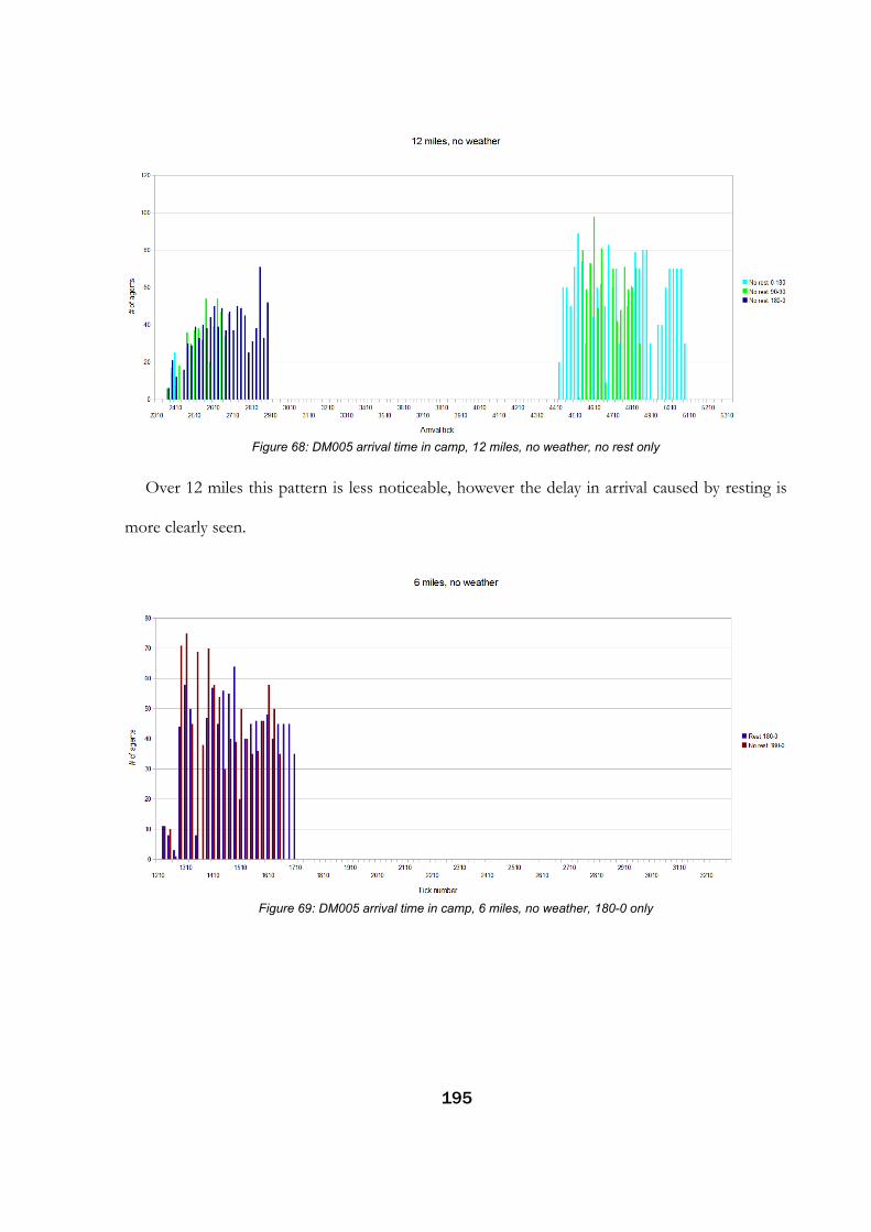
Over 12 miles this pattern is less noticeable, however the delay in arrival caused by resting is

more clearly seen.

195

Figure 69: DM005 arrival time in camp, 6 miles, no weather, 180-0 only

Figure 68: DM005 arrival time in camp, 12 miles, no weather, no rest only

196

Figure 70: DM005 arrival time in camp, 6 miles, no weather, 90-90 only

Figure 71: DM005 arrival time in camp, 6 miles, no weather, 0-180 only

197

Figure 72: DM005 arrival time in camp, 12 miles, no weather, 180-0 only

Figure 73: DM005 arrival time in camp, 12 miles, no weather, 90-90 only

4.10.4 DM005 ConclusionsIn many ways the DM005 scenarios have provided little useful data. The end result however is

a model with more functionality and the same robust nature as that used in previous tests.

Although the model has been run here with less than 2000 agents, it scales up with no functional

problems. As the speed of the agents and the time of day are all translatable to real world units

and the shape of the camp and organisation of the army's movement are more in line with the

information provided in the military treatises we can now use the ABM to investigate real world

scenarios.

4.11 DM006 – The Limits of a Single Column

4.11.1 IntroductionHaving grounded the ABM in real world measurements and ensured there is a plausible

movement model, the model can be used to determine at what point the limits of single column

marching can be reached. It is clear from The Art of Marching that the benefits of marching an

army over multiple routes were well known to military planners. Using the plausible movement

198

Figure 74: DM005 arrival time in camp, 12 miles, no weather, 0-180 only

speed, organisation and behaviours of the agents we can determine at what point the last agent

arriving at camp gets there too late. “Too late” is of course dependent on a variety of variables.

Although we can calculate the amount of daylight on any particular day at any point in Anatolia,

the total amount of daylight is not necessarily the total amount of march time. The Art of

Marching makes clear the ideal situation, that soldiers should have enough sleep and then enough

time both before and after a march to feed themselves and their animals and take care of their

equipment. Nevertheless, for these experiments the maximum time has remained at that of the

previous Day's March scenarios, 12809 ticks representing 13 hours and 16 minutes.

All scenarios were run over either 6 or 12 miles with a variety of numbers of agents from

5301 to 30901. Several aspects were varied for the DM006 scenarios.

4.11.1.1 Army CompositionInitial scenarios were run with all cavalry forces, all infantry (except the central camp sector's

troops representing the Emperor's household), and with cavalry as 20%, 25% and 30% of the

main force.

4.11.1.2 Setting Off DelaysMost scenarios were run with gaps between units setting off of 3, 9 and 483 ticks as described

above. 4 scenarios were run with gaps of 1, 1 and 10 respectively to investigate the effects of

these gaps compared to a situation with virtually no delays between units setting off.

4.11.1.3 Cavalry SpeedIn most scenarios the cavalry speed varied with cavalry units alternating between trotting,

walking and leading their horses. 8 scenarios were run in which cavalry units always travelled at

the trot.

4.11.1.4 March SpacingIn most scenarios, unit leader's attempt to leave a gap of 2 cells (10m) between themselves

199

and the leader of the unit in front. As infantry squads take up less room than cavalry squads it is

possible to reduce this gap to 1 cell (5m) for infantry units. This was done in 4 scenarios.

4.11.2 Work Required

4.11.2.1 Setting OffIn DM005 each unit waited until the preceding unit was closer to the first waypoint by a set

distance before setting off itself. This served to stagger the setting off of the units in order to

avoid crowding outside the camp. In reality this is an unrealistic way of handling the initial

movement of units. In DM006 a unit sets off a set number of ticks after its preceding unit.

There are 3 different delays able to be set, as in DM005. Each of the 5 sectors of the camp have

a delay between the setting off of the last unit and the setting off of the first unit of the next

sector. Each unit itself will have a much smaller gap between it and the unit ahead. In between

there is an intermediate gap that is inserted every X units where X is a number assigned in the

initialisation file. For DM006, each unit sets off 3 ticks after the preceding unit, a delay of around

10 seconds. The first unit of each of the 4 sectors following the central sector will wait 483 ticks

after the last unit of the preceding sector has set off, a delay of 30 minutes. In between these

there is a gap of 9 ticks every 10 units, a gap of about a minute.

200

4.11.3 Results

201

Table 33: DM006 scenario data

Comparing different scenarios is made more complicated due to the difference in squad size

between cavalry and infantry. Cavalry squads consist of an CavalryOfficer and four

CavalrySoldiers whereas infantry squads contain an Officer and nine Soldiers.

This is partly practical as the increased space taken up by cavalry mean that squads with similar

numbers of men would need different flocking parameters for cavalry and infantry. The fact that

100 squads of infantry will consist of twice as many agents as the same number of squads of

cavalry means that another way of comparing arrival times rather than just the average of all

agents was needed. For this reason the average arrival time of officers only was added. As

flocking rules are quite tight this can be taken as an average arrival time of each squad. This

compensates for the increased numbers of agents in infantry squads.

4.11.3.1 Army CompositionExcluding the scenarios dealing with the two extremes of all cavalry and all infantry, it is clear

that the maxim of an army marching as quickly as the speed of its slowest element appears to be

true on a macro scale. Over the course of a day the final arrival time of a force where 25% of

the squads of the main army is comprised of cavalry differs very little from forces composed of

20% or 30% cavalry.

% of squads of main force are cavalry

Last arrival tick

Last arrival time

Average Officer arrival

time

20 12314 18:56 7382

25 12293 18:55 7329

30 12272 18:53 7259

Table 34: Last arrivals in a force of 2000 squads over 6 miles

202

As the number of squads is the same and the setting off delay between each squad is the same

in each scenario the only difference will be due to the speed difference between cavalry and

infantry and will determine how many squads arrive earlier and how many arrive later. This is

illustrated in Figure 75.

4.11.3.2 Setting Off DelaysAs part of DM006 some scenarios have been run with reasonable sounding delays

between each unit setting off and some with hardly any. The ones with hardly any delay result in

massive crowding and consequently take quite a while to run, one having been left running for

over three weeks before being cancelled. This is a quick comparison between the one scenario

that finished compared to the one that's otherwise identical but with a more staggered start.

203

Figure 75: Officer arrival time with 20% cavalry vs 30% cavalry

As part of the regular DM006 scenarios, each unit waits for 3 ticks (10 seconds) after its

preceding unit sets out of camp before it sets out itself. Every 10 units this delay is increased to 9

ticks (30 seconds) to indicate a slightly longer gap between larger organisations of units. Between

each of the 5 sectors of the camp there is a gap of 483 ticks (30 minutes), representing the gap

between the largest organisation of units. This results in an orderly withdrawal from camp with

plenty of space for the delays and holdups expected in an actual army column. By way of

comparison some scenarios were started where the gap between units setting off was 1 tick,

except between the 5 sectors where it was 10 ticks. The results are below.

As can be seen, the scenario with the larger gaps between units arrives later, both on average

and when comparing the last unit to arrive. Looking at the arrival times of the individual agents

we can see a significant difference, even the crowding that resulted is not enough to stop the

agents arriving earlier when there are much smaller gaps between units setting off (red bars =

larger gaps).

204

Table 35: DM006 setting off delays

PC Officers Cavalry Infantry S1 S2 S3 Agents Proc Time

CN22 12 50 50 250 750 3 9 483 Variable 9051 10599 17:09 644 7939 7206 23965 229CN24 12 50 50 250 750 1 1 10 Variable 9051 8414 14:53 715 6396 5901 27627 412

Distance (miles)

Officer Cavalry

Cavalry Speed

Time of Last Arrival

Last Agent to arrive

Time (UTC + 3)

Average arrival time

Average arrival time

(officers only)

Average distance travelled

Average rest ticks

The down side to setting off with smaller gaps between the units can be seen in both the

average distance travelled and the average rest ticks. The units are actually on the road for longer

in scenarios with smaller gaps between units. Crowding makes them cover more ground and, as

they're on the road for longer they accumulate more rest ticks, the 5-10 minutes in every hour's

marching that they spend resting. So reducing the gap between units setting out does mean they

arrive at the following camp earlier, but results in a longer day on the march and more ground

covered. That's all time that could be better spend having a leisurely breakfast, as George

Armand Furse is keen to point out in The Art of Marching.

It is clear from the DM006 scenarios though that once the setting off delays reach the level

where they drastically reduce crowding, particularly just outside the starting camp, then any extra

is for the purposes of the model superfluous and add to the average arrival time in a fairly linear

way. The difference between the model and the real world is that ensuring the army's column was

punctuated by gaps did not just work to avoid crowding but also to cope with any unexpected

delays, something not modelled in DM006.

205

Figure 76: DM006 arrival tick of all agents, different setting off delays

4.11.3.3 Cavalry SpeedAs part of the DM006 scenarios, the movement speed of cavalry is determined by a rota

whereby they spend a certain amount of every hour moving at the trot, a certain amount at the

walk and a certain amount out of the saddle leading their horses. In order to investigate the

effects that movement speed has on the speed of the army as a whole some scenarios have been

run in which the cavalry spend all their time moving at the trot. The agents still spend 5-10

minutes every hour resting in each set of scenarios.

4.11.4 Data

4.11.4.1 The Effects of Increased Cavalry Speed in Cavalry-Only ForcesIncreasing the speed of cavalry agents in a cavalry-only force has the expected effect on both

the average and last arrival time of the agents. Over 6 miles, a force of 5301 cavalry agents will

arrive on average about 420 ticks before agents moving at variable speed. The last agent arrives

518 ticks earlier, just over half an hour. The average arrival time improves by about 10% even

though the average speed increases by much more than this as some of the time is spent resting

and some is spent waiting to set off.

206

Table 36: DM006 total scenario data

PC Officers Cavalry Infantry S1 S2 S3 Agents Proc Time

CN24 6 50 50 250 750 3 9 483 11.66 9051 8184 14:39 521 5711 5096 11932 96CN21 6 100 100 500 1500 3 9 483 11.66 18101 12257 18:52 1464 8015 7165 11822 91CN22 6 50 50 1000 0 3 9 483 11.66 5301 6819 13:14 454 4260 4181 11903 75CN24 6 100 100 2000 0 3 9 483 11.66 10601 10771 17:20 1181 6363 6249 11945 74CN21 12 50 50 250 750 3 9 483 11.66 9051 10572 17:08 634 7832 7076 23773 215CN21 12 100 100 500 1500 3 9 483 11.66 18101 13521 1656 8917 7807 23791 203CN22 12 50 50 1000 0 3 9 483 11.66 5301 7834 14:17 605 5267 5152 23799 110CN24 12 100 100 2000 0 3 9 483 11.66 10601 11808 18:24 1229 7370 7191 23890 110CN23 6 50 50 250 750 3 9 483 Variable 9051 8224 14:42 523 5750 5207 11728 92CN22 6 100 100 500 1500 3 9 483 Variable 18101 12293 18:55 836 8131 7329 12162 99CN23 6 50 50 1000 0 3 9 483 Variable 5301 7337 13:46 418 4680 4605 11833 76CN22 6 100 100 2000 0 3 9 483 Variable 10601 11320 17:54 1014 6804 6683 12080 76CN22 12 50 50 250 750 3 9 483 Variable 9051 10599 17:09 644 7939 7206 23965 229CN25 12 100 100 500 1500 3 9 483 Variable 18101 13512 1575 9088 8065 24010 230

Distance (miles)

Officer Cavalry

Cavalry Speed

Time of Last Arrival

Last Agent to arrive

Time (UTC + 3)

Average arrival time

Average arrival time

(officers only)

Average distance travelled

Average rest ticks

As we can see from the arrival graph, the pattern is much the same, just shifted to the left

when all agents move at the trot all the time. Negative factors that may result from increased

speed such as increased chance of injury and increased energy expenditure are not modelled in

this scenario.

4.11.5 The Effects of Increased Cavalry Speed in Mixed ForcesLess immediately obvious is the difference in movement that increased cavalry speed makes

on forces combining cavalry and infantry. As the cavalry lead the column and the time that units

set off is dependant on the setting off time of the preceding unit and not the progress made, the

arrival of the infantry units is substantially unchanged by the speed of the cavalry.

207

Figure 77: DM006 effects of increased speed on cavalry-only forces

As before, the cavalry arrive earlier but the infantry arrive at pretty much the same time. In

terms of overall army movement speed no benefit is gained. The increased gap between the

cavalry and infantry may allow more time for problems in the cavalry part of the army to be

sorted out before the infantry are held up but the increased speed will probably result in a higher

chance of delays due to horse or rider injury. The only net gain is that the cavalry spend more

time resting at the destination. This has to be factored against the fatiguing effects of moving

constantly at the trot as mentioned in The Art of Marching.

By way of summary, it's said that an army moves at the speed of its slowest element. This is

true at the macro scale but as far as individual agents in a mixed force are concerned, as long as

the order of march is properly organised an army marches at a variety of speeds. The speed of

the foremost elements, providing they are faster than those at the rear, is probably dictated more

by comfort the desired speed of the army as a whole.

208

Figure 78: DM006 effects of cavalry speed in mixed forces

4.11.5.1 March SpacingThe parameter that specifies the distance between Officers on the march is referred to as

march spacing. On the main part of the march where each unit is merely following the one on

front, each officer checks whether the distance between himself and the preceding Officer

exceeds the march spacing value. If it does, the Officer moves towards the preceding

Officer until he is within the march spacing value (subject to speed constraints, obviously). In

all scenarios prior to DM006 the march spacing value has been set to 2, corresponding to 10m.

This is a reasonable value where cavalry is concerned as a cavalry squad will usually be spread

over 2 cells. Infantry however can comfortably fit in 1 cell and so some scenarios were run in

which infantry used a value of 1 for march spacing, ensuring each infantry Officer attempts

to stay 5m from the preceding Officer. The differences caused by this change were not

obvious from the tabulated data so arrival time graphs were produced (figures 79 & 80).

209

Figure 79: DM006 arrival time over 6 miles

As can be seen, no significant difference exists between the two results, either with 1050 or

2100 squads or over 6 or 12 miles. This can be explained by the generous nature of the setting

210

Figure 80: DM006 arrival time over 12 miles

Figure 81: DM006 column of infantry units with march spacing = 1

off delays. As the gaps between units ensure there is no significant crowding, the reduction in

march spacing manifests itself mainly as a desire for each Officer to be closer to the one in

front. Without the ability to alter its speed, however, all the Officer can do is keep pace with

the preceding unit until a rest period. As each rest period allows each Officer to catch up with

the Officer in front (providing that Officer is not also doing the same and ends up taking

the minimum amount of rest) this then causes problems for the Officer behind. Looking at

the Blender files created by these scenarios it seems that reducing the march spacing without also

reducing the setting off delays results in more clumping of the army column but no increase in

throughput (figures 81 & 82).

Looking at both these columns it seems that if the units set out with smaller gaps between

them then more units should be able to be marched in a single column in a day under the

211

Figure 82: DM006 The same tick with the same parameters except march spacing = 2

conditions of the DM006 scenarios.

4.11.6 DM006 ConclusionUnder the conditions of the DM006 scenarios the army composition, providing it is within

historically plausible values, will have an insignificant effect on the overall speed of the army. This

is because the last units to arrive will, providing sufficient gap is left to cope with crowding or

holdups, only be able to move at a certain speed, not constrained by preceding, faster, units.

Obviously this is provided the slowest units will be at the rear of the column but the benefits of

this approach seem so obvious that it must have been the norm where practically possible. The

composition of the army merely dictates how many units arrive earlier than the infantry. This

raises a broader point regarding historical accounts, when a writer mentions that an army arrives

at a particular time or even on a particular day, who exactly are they talking about? It is not hard

to envisage from the results so far that a Byzantine army of 40,000 - 70,000 will have spent a

certain amount with some sections travelling a day or two (or even three or four) behind the head

of the column. Taking stragglers into account, the tail of the army may well have stretched some

way behind on the route.

From a technical point of view, the scenarios run with virtually no gaps between the units

didn't perform well. One crashed, two ran so slowly that one had to be cancelled to make room

for other scenarios, the other was left running and just over halfway to completion 17 days after it

was started. It's clear that the model doesn't cope with extreme crowding well. The one scenario

that did run emphasised the point that in a situation where the army moves as a single column,

one unit abreast, some sort of system to introduce gaps between units is essential. Further

scenarios are needed in order to distinguish some variation between the apparently generous gaps

of the majority of DM006 scenarios and the unworkable free for all that results from having

212

hardly any gaps at all.

The stated aim of DM006 was to find the maximum number of agents able to travel in a

single column on a single day. What has actually been achieved is a more complete understanding

of the factors involved in moving the maximum number of people in a single day. It is clear that

the gaps between units setting off has a clear effect on the arrival time of units. March spacing is

only important if the gaps between units are small enough for there to be enough of a backlog to

enable units to march closely to each other. We have seen from previous sets of scenarios though

that the closer the units are to each other the more chance of crowding and the resulting increase

in travel time and distance. So there is a direct tradeoff between the number of troops able to

travel in a single column on a single day and the ease of that journey. A subsequent set of

scenarios is planned to establish an absolute theoretical maximum for a day's march in a single

column, using the maximum amount of daylight found on the route.

4.12 DM006a – The Limits of a Single Column

4.12.1 IntroductionThis document details the planned experiments for DM006, the Day's March scenarios that

will attempt to determine at which point in the model the limits of the single column method of

marching are reached. This is a supplement to the scenarios in DM006 as, while being

informative in many areas, they did not highlight the specific limits of the single column over a

number of march distances with variable army sizes. Where all agents arrived in camp before

sunset in our 13 hour and 16 minute day, the amount of excess time represents the amount of

time between sunrise and the first agent setting out plus the amount of time between the final

agent arriving and sunset.

213

4.12.2 Data

214

Table 37: DM006a total scenario data

4.12.3 Results

4.12.3.1 6 MilesOnce again the value given to cavalry spacing had little effect on the results of the model.

Over 6 miles, all sizes of armies finished well within the allotted time. 27151 agents completed

the 6 mile march with 2041 ticks to spare, representing about 2 hours and 6 minutes. Given that

some time would be required before and after the march of the army to allow the first units to

have breakfast and the final units to set up their tents and cook food, this represents the practical

limits of moving the modelled army via a single column over 6 miles.

4.12.3.2 12 MilesOver 12 miles, the last arrival in the model with 18101 agents was at a similar time to that of

the 6 mile march with 27151 agents. 18101 agents marched 12 miles in a single column with 2

hours and 20 minutes to spare, a similarly plausible amount of spare time during our typical 13

hour 16 minute day. Taking things to their absolute maximum, 26211 agents were able to make it

to their camping locations before sunset although this assumes a daybreak start and an arrival at

215

Figure 83: DM006a last time of arrival

sunset.

4.12.3.3 15 MilesOver 15 miles, 18101 agents were able to make it to camp, but with only 1071 ticks to spare.

This represents 1 hour and 6 minutes, just within the limits of plausibility for the total spare time

in a day's march. It is more likely that, unless circumstances dictated otherwise, a longer gap was

required and 18101 agents would be above the number commonly attempted to be marched on a

single column during a day. A special run of the model was completed with 27151 agents over 15

miles with a maximum number of ticks representing the amount of daylight at Sebastea in the

middle of June, 14449 ticks. The army in this model finished with 260 ticks to spare, just 16

minutes. This represents a good theoretical maximum for an army marching using our rules over

15 miles.

4.12.4 DM006a ConclusionsThere are significant differences between our model and an actual army on the march. There

are no mules or pack animals in this series of scenarios. The single column movement

represented here does not allow for two units walking abreast, a situation that may have been

possible in open ground or on major roads. There is also no account made for the bank and ditch

that would have surrounded the camp. These factors must be taken into account when

interpreting these results. Nevertheless, these scenarios give a rough indication of how many

agents could be moved within a single day under different circumstances.

4.13 DM007 – Multiple Columns

4.13.1 IntroductionThe DM007 scenarios will model a system whereby the army is split into two or three

216

columns and require these to use separate routes to march to the next camp. This will allow us to

examine the circumstances in which splitting the army may be beneficial to the army as a whole.

All multiple column scenarios were processed with cavalry spacing set to 2 and with gaps of 2, 5

and 200 as per most of the DM006a scenarios.

4.13.2 Work RequiredThe only differences between this model and the DM006a model is that it is possible to set

the number of columns that the army can split itself into. When the number of columns is set at

1 the model behaves exactly the same as DM006a. When the number of columns is set to two or

three then the model separates the army into two or three different columns. The first column

will have the ColumnLeader agent at its head, the other one or two will have an ordinary

Officer agent who, for the purposes of route planning, behaves like a ColumnLeader. The

army is broken down by sector with each sector heading for a waypoint outside camp depending

on the overall direction of travel and the number of columns. The second waypoint is always

closer to the destination camp than the third so the new routes become longer as the number of

columns increases. As can be seen from the following figures, having five sectors to the camp

does not result in an even number of squads in each column but this is likely to have been the

case in reality as the organisational structure would have been kept in place and the columns built

around that, rather than the other way round. As they use different waypoints outside the camp,

each column can set off at the start of the day, it does not have to wait until any of the other

columns has moved out before it moves itself. Within each column the same movement rules

apply as in previous models, where each unit, collection of units and sector has a gap set between

its own setoff time and that of the unit preceding it.

217

218

Figure 84: 2 columns with the overall direction of travel being east. The numbers indicate the order

in which the sectors set out.

Figure 85: 3 columns travelling East

The leader of each column plans a route to the corresponding waypoint outside the

destination camp, as seen in Figure 88.

219

Figure 86: 2 columns travelling South East

Figure 87: 3 columns travelling South East

This selection of waypoints helps ensure that the separate columns do not cross each other

unless the terrain forces columns to use the same route. Due to the relatively flat terrain between

Nikaia and Malagina no such situation exists in the DM007 scenarios. The same distribution of

units was used as in DM006a, with the central sector of the camp consisting of the

ColumnLeader, a number of Officers equal to 5% of the total squads in the main part of

the army and a number of Officer cavalry squads also equal to 5% of the total squads of the

main part of the army. The numbers of agents corresponds to the following numbers of squads.

Total number of squads Number of agents

1100 9051

2200 18101

3300 27151

Table 38: Conversion between number of squads and number of agents

220

Figure 88: The selection of destination waypoints

4.13.3 Data

221

Table 39: DM007 total scenario data

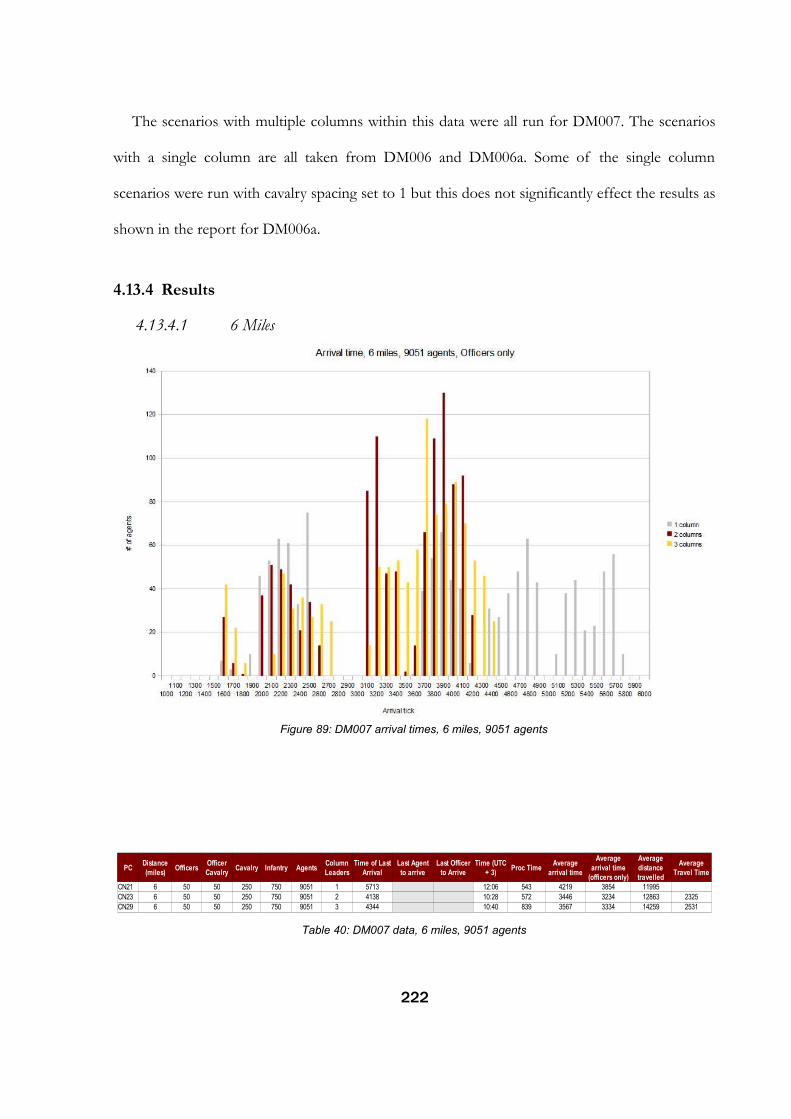
The scenarios with multiple columns within this data were all run for DM007. The scenarios

with a single column are all taken from DM006 and DM006a. Some of the single column

scenarios were run with cavalry spacing set to 1 but this does not significantly effect the results as

shown in the report for DM006a.

4.13.4 Results

4.13.4.1 6 Miles

222

Table 40: DM007 data, 6 miles, 9051 agents

PC Officers Cavalry Infantry Agents Proc Time

CN21 6 50 50 250 750 9051 1 5713 12:06 543 4219 3854 11995CN23 6 50 50 250 750 9051 2 4138 10:28 572 3446 3234 12863 2325CN29 6 50 50 250 750 9051 3 4344 10:40 839 3567 3334 14259 2531

Distance (miles)

Officer Cavalry

Column Leaders

Time of Last Arrival

Last Agent to arrive

Last Officer to Arrive

Time (UTC + 3)

Average arrival time

Average arrival time

(officers only)

Average distance travelled

Average Travel Time

Figure 89: DM007 arrival times, 6 miles, 9051 agents

As can be seen from the arrival time with 9051 agents over 6 miles (Figure 89), using both two

and three columns have advantages over just one column. They both result in the last agent

arriving before the last agent in the single column model. With only one column the whole force

still arrives at the destination camp before half of the available daylight is gone though. With this

amount of wiggle room, it would be down to the individual commander to decide whether the

extra complication of using two or three columns was worth any benefits to be gained from the

earlier arrival time. As can be seen from the graph, splitting the army into two columns results in

a faster overall arrival than splitting into three columns. This is a result of more agents taking a

suboptimal route and therefore travelling further. The extra distance travelled by the third column

pushes the average distance travelled up by over a kilometre.

223

Figure 90: DM007 arrival times, 6 miles, 18101 agents

If the number of agents is doubled then we see real benefits towards splitting the army into

separate columns (Figure 90). The final agent arrives in around two thirds the time as if one

column was used, more than two and a half hours' difference. In this set of scenarios the

difference between 2 and 3 columns is less that with 9051 agents, the added size of the army

making splitting into more columns more worthwhile. The one column army still arrives in plenty

of time though, although it would take fewer unforeseen holdups along the way to cause the final

few agents to arrive close to sunset.

224

Table 41: DM007 data, 6 miles, 18101 agents

PC Officers Cavalry Infantry Agents Proc Time

CN22 6 100 100 500 1500 18101 1 8316 14:47 1460 5725 5188 12187CN21 6 100 100 500 1500 18101 2 5564 11:56 1447 4142 3909 12774 2363CN25 6 100 100 500 1500 18101 3 5457 11:50 1520 4189 3927 14051 2590

Distance (miles)

Officer Cavalry

Column Leaders

Time of Last Arrival

Last Agent to arrive

Last Officer to Arrive

Time (UTC + 3)

Average arrival time

Average arrival time

(officers only)

Average distance travelled

Average Travel Time

Figure 91: DM007 arrival times, 6 miles, 27151 agents

With 27151 agents the situation becomes more complicated (Figure 91). The scenario with

two columns has a much earlier last time of arrival than the three column force, something

unexpected if the overall pattern were to be that the larger the force the more useful three

columns would become. The reason for this is clearly seen in the tabular data. There is a large

increase in the average distance travelled with three columns. There may be something about the

third route that makes it prone to crowding once a certain number of agents is sent down it. One

benefit of this is that there is less of a concentration of squads arriving at the same time, as seen

in the massive spike of the two column data around tick number 5700.

4.13.4.2 12 Miles

225

Table 42: DM007 data, 6 miles, 27151 agents

PC Officers Cavalry Infantry Agents Proc Time

CN25 6 150 150 750 2250 27151 1 10768 17:20 3846 7223 6524 12291CN22 6 150 150 750 2250 27151 2 6851 13:16 3564 4918 4674 12717 2489CN24 6 150 150 750 2250 27151 3 7939 14:24 4818 5266 5018 15242 3147

Distance (miles)

Officer Cavalry

Column Leaders

Time of Last Arrival

Last Agent to arrive

Last Officer to Arrive

Time (UTC + 3)

Average arrival time

Average arrival time

(officers only)

Average distance travelled

Average Travel Time

Figure 92: DM007 arrival times, 12 miles, 9051 agents

Over 12 miles we see a similar pattern to that over 6 miles (Figure 92), having two columns

shows an improvement over having 3 columns. Due to the increased time taken to march 12

miles the benefits of splitting the army into multiple columns starts to be felt even with smaller

numbers of troops. Over 12 miles there is less difference between the second and third routes in

length. This can be explained by the 12 mile camps being more aligned with the diagonal

organisation of the waypoints than the 6 mile camps which are off centre.

226

Table 43: DM007 data, 12 miles, 9051 agents

PC Officers Cavalry Infantry Agents Proc Time

CN21 12 50 50 250 750 9051 1 7935 14:24 776 6344 5845 24052CN23 12 50 50 250 750 9051 2 6534 12:57 624 5675 5314 24997 4407CN25 12 50 50 250 750 9051 3 6665 13:05 664 5800 5467 25807 4665

Distance (miles)

Officer Cavalry

Column Leaders

Time of Last Arrival

Last Agent to arrive

Last Officer to Arrive

Time (UTC + 3)

Average arrival time

Average arrival time

(officers only)

Average distance travelled

Average Travel Time

Figure 93: DM007 arrival times, 12 miles, 18101 agents

Over 12 miles, 18101 agents show a distinct preference for three columns with 449 ticks

between the last agent to arrive in the three column model compared to the two column model

(Figure 93). That's still only around 28 minutes but as arrival times are approaching the end of

the day the possibility of hold ups making those minutes more important increases.

227

Table 44: DM007 data, 12 miles, 18101 agents

PC Officers Cavalry Infantry Agents Proc Time

CN22 12 100 100 500 1500 18101 1 10548 17:06 1562 7864 7182 24011CN29 12 100 100 500 1500 18101 2 8246 14:43 4760 6539 6213 25259 4667CN23 12 100 100 500 1500 18101 3 7797 14:15 1580 6417 6093 25571 4756

Distance (miles)

Officer Cavalry

Column Leaders

Time of Last Arrival

Last Agent to arrive

Last Officer to Arrive

Time (UTC + 3)

Average arrival time

Average arrival time

(officers only)

Average distance travelled

Average Travel Time

Table 45: DM007 data, 12 miles, 27151 agents

PC Officers Cavalry Infantry Agents Proc Time

CN21 12 150 150 750 2250 27151 1 26211 3206 4203 9204 8360 24196CN21 12 150 150 750 2250 27151 2 9690 16:13 5979 7492 7182 25292 4999CN25 12 150 150 750 2250 27151 3 8937 15:26 3753 7102 6790 25685 4919

Distance (miles)

Officer Cavalry

Column Leaders

Time of Last Arrival

Last Agent to arrive

Last Officer to Arrive

Time (UTC + 3)

Average arrival time

Average arrival time

(officers only)

Average distance travelled

Average Travel Time

Figure 94: DM007 arrival times, 12 miles, 27151 agents

When 3300 squads are used, multiple columns become the only way all agents can arrive at the

destination camp before sunset (Figure 94). The difference between the last arrivals of the two

and three column scenarios is 753 ticks (nearly 47 minutes). Also noticeable are the peaks where

at times over 160 squads are arriving in camp in a 100 tick period. That equates to 1600 infantry

agents within six minutes, surely causing some organisational problems within camp.

4.13.4.3 15 miles

Over 15 miles with 9051 agents the difference in speed between cavalry and infantry shows

itself almost as clearly with multiple columns as it does with a single column (Figure 95). The

longer the march, the more capacity there is for route planning to extend the difference in

journey lengths. All agents are still arriving well within the available daylight for marching,

228

Table 46: DM007 data, 15 miles, 9051 agents

PC Officers Cavalry Infantry Agents Proc Time

CN24 15 50 50 250 750 9051 1 9129 15:38 618 7501 6948 30064CN22 15 50 50 250 750 9051 2 7767 14:13 612 6908 6571 30820 5663CN21 15 50 50 250 750 9051 3 7830 14:17 664 6866 6516 31349 5713

Distance (miles)

Officer Cavalry

Column Leaders

Time of Last Arrival

Last Agent to arrive

Last Officer to Arrive

Time (UTC + 3)

Average arrival time

Average arrival time

(officers only)

Average distance travelled

Average Travel Time

Figure 95: DM007 arrival times, 15 miles, 9051 agents

whichever model is used 15 miles seems a perfectly reasonable marching distance for a force of

this size given the conditions within the model.

A similar situation exists within this set of scenarios as in the largest scenarios with a 6 mile

march (Figure 96), some crowding exists in the three column model that increases the average

distance travelled and final arrival time. Once again the three column scenario exhibits a more

regular pattern of arrival, possibly leading to fewer crowding problems in the destination camp.

229

Table 47: DM007 data, 15 miles, 18101 agents

PC Officers Cavalry Infantry Agents Proc Time

CN23 15 100 100 500 1500 18101 1 11731 18:20 1734 9041 8337 30147CN23 15 100 100 500 1500 18101 2 9015 15:31 1766 7671 7334 30789 5788CN21 15 100 100 500 1500 18101 3 9388 15:54 2162 7701 7343 31992 6006

Distance (miles)

Officer Cavalry

Column Leaders

Time of Last Arrival

Last Agent to arrive

Last Officer to Arrive

Time (UTC + 3)

Average arrival time

Average arrival time

(officers only)

Average distance travelled

Average Travel Time

Figure 96: DM007 arrival times, 15 miles, 18101 agents

Whatever crowding problems there are with the third route they aren't severe enough to make

up for the lack of bandwidth in the two column scenario (Figure 97). The average distance

increases with three columns but the time of last arrival is still earlier, albeit only by 19 minutes.

By this point it is clear that splitting the army into separate columns is the only way to get 27151

agents over 15 miles in our representative day. Barring unforeseen events it would just be possible

to move such a force with enough time to make breakfast in the morning and set up camp in the

evening.

4.13.5 DM007 ConclusionsWhile the army is still modelled at a fairly abstract level, the DM007 scenarios allow us to draw

conclusions regarding the movement of the army in separate columns. There is clearly a benefit

230

Table 48: DM007 data, 15 miles, 27151 agents

PC Officers Cavalry Infantry Agents Proc Time

CN24 15 150 150 750 2250 27151 1 20771 2662 9545 8645 30189CN22 15 150 150 750 2250 27151 2 10423 16:58 4464 8529 8226 30963 6042CN23 15 150 150 750 2250 27151 3 10106 16:39 5651 8250 7900 31732 6030

Distance (miles)

Officer Cavalry

Column Leaders

Time of Last Arrival

Last Agent to arrive

Last Officer to Arrive

Time (UTC + 3)

Average arrival time

Average arrival time

(officers only)

Average distance travelled

Average Travel Time

Figure 97: DM007 arrival times, 15 miles, 27151 agents

to splitting the army into columns when looking at the last agent to arrive in the following day's

camp. Only if the second or third routes were much longer or more arduous would the last agent

arrive later than it would with a single column. This may be the case in mountainous areas but

not in the relatively flat terrain between Nikaia and Malagina. The time of arrival of the last

agent, while important, is not the only factor to be considered when deciding how many columns

to split the army into.

Marching in a single column may result in later arrival times but it also ensures that excessive

numbers of agents do not arrive at the destination camp at the same time. There is a real density

about the arrival times of both the two and three column models that is absent from the single

column scenarios. Properly organised this would not necessarily cause problems at the

destination camp as the camping locations would be suited to the direction from which the units

are arriving. However this would make actions within camp such as watering the horses and

digging the surrounding bank and ditch more difficult with arriving units possibly getting in the

way. The single column model with agents arriving via a single direction would make organisation

of tasks within camp simpler. One of the other advantages of splitting the army into separate

columns is that the army is quicker at forming up into battle order. That this is likely to be the

case can be seen quite easily from the arrival graphs. This however is not a factor on the

Manzikert march as the Seljuks were thought to be too far away to pose a threat even up to the

Byzantines' arrival at Manzikert.

Another pattern apparent from the results is that with the army split into multiple columns the

gap between the cavalry and infantry's arrival is less pronounced. This is due to the infantry not

having to wait in the starting camp until the cavalry set off. This may manifest itself in a greater

feeling of equality between the cavalry and infantry units. In the MWGrid ABM the cavalry head

231

the column, this is to ensure the slower moving infantry do not unduly hold up the cavalry. When

marching in a single column this may generate a certain amount of bad feeling within the infantry

units, especially the ones arriving in camp earliest, when they see the cavalry already camped, fed

and rested. This feeling will no doubt be magnified if the infantry have had to march through the

heat of the day because they had to wait for the cavalry to leave. It is also likely that it is the

infantry that will have to dig the bank and ditch surrounding the camp, the cavalry being of

generally higher status. The earliest infantry units to arrive are more likely to have to bear the

greatest burden in constructing the camp.

This gap between cavalry and infantry is less pronounced in the scenarios with multiple

columns as the infantry can start straight away, the only gap being caused by the difference in

speeds and the length of route. Furse notes in The Art of Marching (Furse 1901) that when

splitting columns the infantry should go via the shortest route and the cavalry by the longer. This

is not modelled here but would cut the gap between the cavalry and infantry even further, maybe

even ensuring the infantry arrive first if the difference between route lengths is enough. Although

this may increase any crowding issues with arriving at camp it would surely improve the morale

of the infantry.

In reality, splitting the army can happen over the course of a day or for much longer. Splitting

the army for more than a day would create a series of parallel single column armies that would

have to join up at some later point on the route. This will be considered in the DM008 scenarios.

In addition to the historical factors, one significant technological aspect of splitting the army

into camps is worth mentioning. The size of the processed tickfile is increased as more agents

can be on the move at the same time. Whereas with a single column it is unlikely to have a

processed tickfile of over 800Mb, the ones containing multiple columns are all over 1Gb. This

232

not only increases required storage space but also results in longer Blender processing times and

larger Blend file sizes (see DM003).

4.14 DM008 – The March to Manzikert

4.14.1 IntroductionThe Day's March 008 scenarios deal with the specific context of the Byzantine army's march

across Anatolia to the fortress at Manzikert in AD 1071. In order to use the model to examine

the specific circumstances of the army's march to Manzikert the relatively generic models used so

far will have to deal with specific information about the campaign. As detailed in chapter 1, we

do not know the size of the Byzantine army but a plausible hypothetical force and route of

march have been supplied by John Haldon and detailed below. It is this force that will be used for

the DM008 scenarios. These scenarios will provide new evidence of the organisation required to

move the army over 700 miles as the crow flies in around 6 months. Although there is

insufficient time to model the army on each day of it's march, three sample points of the route

are used to illustrate the issues faced by the army at different points along the route. The model

still lacks some important factors, the army is modelled without any baggage or baggage handling

mechanisms for example. This will, however, give an optimistic estimate, a null hypothesis against

which we can compare reality. If the hypothetical army without baggage cannot reach its

destination in time, what hope for the real-world Byzantine army with mules, extra horses and the

like?

The setting off delays between units have been set to the reasonably generous 3/9/483 ticks

used in DM006.

233

4.14.2 Work Required

4.14.2.1 RouteA hypothetical route for the Manzikert campaign based on the fragments of information

contained in historical accounts, the Tabula Imperii Byzantini maps and other relevant sources has

already been produced (Haldon 2006, 9). This is the route that will be assumed for the purposes

of our model. It starts at Nicomedia based on an assumption that sea travel would have been

used from Constantinople up until that point. It then passes through Nikaia, Malagina,

Dorylaion, Ankyra, Charsianon, Sebastea and Theodosiopolis before arriving at Manzikert

(Figure 98). This route totals around 1,110 miles in length and encompasses a wide variety of

elevations (Table 51).

4.14.2.2 Army CompositionThe Byzantine army was made up of a variety of different troop types in differing

proportions and any attempt to produce precise numbers will necessarily be highly speculative.

Working from data provided by John Haldon a hypothetical army has been produced, consisting

of different types of troops joining the campaign at different locations (Table 49).

234

Figure 98: The hypothetical route of the Byzantine army to Manzikert

Within this hypothetical army, the following units join at the following locations:

Constantinople - The units from the palace leave Constantinople with the Emperor. These

are the Hetaireia, Scholai, Stratelatai and the Varangians.

Nicomedia - Pecheneg mercenaries and Balkan allies.

Malagina - Frankish mercenaries under Roussel de Bailleul, German and Oghuz mercenaries,

units from Bulgaria the thematic tagmata from Bithynia and the five tagmata of the west.

Dorylaion - Thematic tagmata from the Anatolikon theme.

Charsianon - Thematic tagmata from Cilicia.

Sebastea - Thematic tagmata from Cappadocia, Koloneia, Charsianon, Armeniakon along

with the Armenian infantry.

Theodosiopolis - Thematic tagmata of Chaldia plus the tagmata from Syria.

In addition to this, the German mercenaries were sent back at Krya Pege, between Dorylaion

and Charsianon, and the army was split in two between Theodosiopolis and Manzikert with half

the force being sent to Khliat.

Leg of route Distance (km) Cavalry Infantry

Constantinople - Nicomedia boat 3,000 -

Nicomedia - Malagina 90 5,000 2,000

Malagina - Dorylaion 114 9,000 10,000

Dorylaion - Charsianon 699 9,250 10,750

Charsianon - Sebastea 128 9,500 11,500

Sebastea - Theodosiopolis 552 10,500 16,500

Theodosiopolis - Manzikert 204 11,250 20,750

Table 49: DM008 hypothetical army with route distances

Nomadic and Frankish mercenaries would have differed from Byzantine units with the

235

Emperor's household being of a different character than the thematic tagmata. Within the model

we have assumed that Frankish and nomadic troops are represented solely by cavalry along with

the Emperor's household. Other Byzantine troops have 25% cavalry and 75% infantry. Armenian

and Balkan troops comprise solely of infantry. The number of Officers in the central sector is

represented by 5% of the number of squads in the army as a whole. This covers high ranking

officers and bureaucratic elements along with their servants.

4.14.2.3 Weather and DaylightThe amount of daylight within which the army had to move would have differed as it crossed

Anatolia. Although the differences in latitude are fairly minor, the march took almost 6 months

and would have resulted in considerable variation in the number of daylight hours. The values

recorded in Table 50 are based on data from the Australian Government

(http://www.ga.gov.au/geodesy/astro/sunrise.jsp) and are for dates in AD 2010.

4.14.2.4 TimingThere are few fixed temporal points on the Manzikert campaign. We know that the Emperor

left Constantinople in late February or early March, had reached Theodosiopolis by late June and

fought the battle at Manzikert on August 26th, very soon after arrival. If we take the 1st of

March as the start date and the 30th June to represent late June we have 122 days from leaving

Constantinople to arriving at Theodosiopolis and 56 days from that point to arriving at

Manzikert on the day before the battle. It seems almost certain that the army spent some time at

Theodosiopolis as Skylitzes Continuatus records a major strategic discussion at which the

decision to move on to Manzikert was made (Friendly 1981, 171). He also records that the order

was given to gather 3 months worth of supplies. Engels' work shows (1978, 20) that this cannot

have included food for the whole three months but it does at least indicate that the stop at

Theodosiopolis was more than just a flying visit.

236

Location Co-ordinates Date Sunrise (UTC +3)

Sunset (UTC +3)

Minutes of daylight

Ticks @ 3.729 secs/tick

Nicomedia (Izmit)

40° 46'N, 29° 55'E 01/03/10 07:35:00 18:51:00 676 10877

Ankyra (Ankara)

39° 52'N, 32° 52'E 15/04/10 06:11:00 19:27:00 796 12809

Ankyra (Ankara)

39° 52'N, 32° 52'E 15/05/10 05:34:00 19:57:00 863 13886

Sebastea (Sivas)

39° 45'N, 37° 01'E 01/06/10 05:06:00 19:54:00 888 14288

Sebastea (Sivas)

39° 45'N, 37° 01'E 15/06/10 05:04:00 20:02:00 898 14449

Theodosiopolis (Erzurum)

39° 54'N, 41° 16'E 01/07/10 04:51:00 19:48:00 890 14320

Theodosiopolis (Erzurum)

39° 54'N, 41° 16'E 01/08/10 05:14:00 19:29:00 855 13757

Manzikert (Malazgirt)

39° 48'N, 42° 19'E 26/08/10 05:34:00 18:53:00 799 12856

Table 50: Sunrise and sunset times used in DM008

237

Figure 99: The size of the hypothetical army as it progresses towards Manzikert

Location Environment Co-ordinates

Elevation (m above sea level)

Nicomedia 34600,27200 6

Nikaia 30000,34500 74

Malagina 35800,37200 221

Dorylaion 44200,49400 799

Ankyra 85400,45600 964

Charsianon 139000,49900 1166

Sebastea 155800,50500 1244

Theodosiopolis 232900,46400 1885

Manzikert 250000,63900 1478

Table 51: The location of settlements visited by the army using the ABM's environmental co-ordinate system

4.14.2.5 Movement CostsUp until now the cost of moving was calculated based on the 2D distance between two

points, even though the actual distance travelled was calculated in three dimensions. This had the

effect that agents would travel comparatively quicker on slopes than they did on flat terrain. This

would not have caused significant inaccuracy in scenarios run up until this point due to the flat

nature of the terrain between Nikaia and Malagina, although it certainly would do in the more

undulating areas to be modelled.

4.14.2.6 HealthThe number of kilocalories expended by movement during the model is now being calculated

for each agent. This is updated every minute of simulation time as the equations used to calculate

this are based on millilitres of O2 per kilogram of body weight per minute. Each minute the

ABM calculates the distance travelled within that minute. It also compares the current height with

the previous height. It applies these to the equation detailed in chapter 2. The calculations for

infantry are exactly as described previously. A further step was required to remove a source of

variability in the data for riding horses.

238

Rider Walk - VO2

(litres per minute)

Trot - VO2

(litres per minute)

Weight (kg)

Walk (ml per kg per min)

Trot (ml per kg per min)

1 1 1.85 77 12.99 24.03

2 0.56 1.4 54 10.37 25.93

3 0.72 1.55 58 12.41 26.72

4 0.6 1.17 48 12.5 24.38

5 0.64 1.43 54 11.85 26.48

Mean 0.7 1.48 58.2 12.02 25.51

Table 52: Energy expenditure of horse riders and the conversion to ml/kg/min (after Devienne and Guezennec 2000)

These values specified in chapter 2 are in litres of O2 per minute and already have the weight

of the rider taken into account. The weight of the rider does make a difference though. As can

be seen in Table 52, considerable variability exists between riders. I have added the weights of the

individual riders and from this, calculated VO2 in millilitres per kilogramme of rider weight per

minute. By extracting ml/kg/min figures from the l/min averages given in the paper, it is possible

to remove the variability caused by the rider's weight. For this reason the mean of the ml/kg/min

figures will be used instead of the mean of litres per minute.

Within the source data there also exists considerable variability between horses with some

requiring more energy to be expended by the rider than others (Devienne and Guezennec 2000,

501). As there is no study which allows us to estimate the implications of this to the MWGrid

ABM it has been omitted but is noted here for completeness.

239

4.14.2.7 Nicomedia to MalaginaThe journey between Nicomedia and Malagina would only have been around 55 miles (90 km)

and would have been broken into two sections at Nikaia, "one of the greatest Byzantine cities"

(Kazhdan et al. 1991, 1463). It is obviously impractical to travel all the way from Nicomedia to

Malagina in a day, but our model indicates that even Nicomedia to Nikaia, a distance of 27 miles

along the road, would have been a challenge for our hypothetical army. The army of 7061 agents

was marched from Nicomedia to a point halfway between it and Nikaia. Both 1 column and 3

columns were tried and the data recorded below.

240

Figure 100: North West Anatolia, with the hypothetical route marked in blue

As can be seen, the last agent in the three column army reaches its destination at tick number

8197, approximately three quarters of the way through the available daylight. This represents a

sensible movement distance given the need for some time at the start of the march to ensure

everyone gets packed up and has something to eat. With only one column, likely considering the

probability of a good road between Nicomedia and Nikaia, the infantry are just arriving at the

destination camp as the sun sets. As this is the first day's march of the whole Manzikert campaign

the distance attempted may have contained more than a measure of guesswork although the size

241

Table 53: Aggregate data from Nicomedia heading towards Nikaia

1 column 3 columns

Average arrival time 7792.2 6446.21 6581.8Average distance covered 24823.62 27009.46 25761.91Average arrival time (Officers only) 7166.73 6156.22 6471.52Last arrival tick 10877 8197 10797Squads 1260 1260 1061Agents 7061 7061 5071Column Leaders 1 1 1Cavalry Officers 1060 1060 1060Infantry Officers 200 200 1Cavalry Soldiers 4000 4000 4000Infantry Soldiers 1800 1800 9

Average Calories Expended 1423.32 1480.98 1394.4

Average travel time 4038.72 4876.69 3902.28

Column Leader cals 1225 1037.36 1225

Cavalry Officer average cals 1354.1 1252.1 1354.1Cavalry Officer high cals 1508 1467.06 1508Cavalry Officer low cals 1193 1056.64 1193

Cavalry Soldier average cals 1404.23 1288.15 1404.23Cavalry Soldier high cals 1598 1447.48 1598Cavalry Soldier low cals 1191 1087.22 1191

Infantry Officer average cals 1496.13 1983.8 1749Infantry Officer high cals 1749 2041 1749Infantry Officer low cals 1260 1948 1749

Infantry Soldier average cals 1498.53 1988.64 1750Infantry Soldier high cals 1750 2110 1750Infantry Soldier low cals 1271 1956 1750

# of agents on last arrival tick 1287 9 9# of agents on last arrival tick – 1 624 0 0# of agents on last arrival tick – 2 60 0 0# of agents on last arrival tick – 3 19 0 0

1 column without

unfinished

of the force at this point will most likely have been one which the Emperor would have had

experience dealing with.

So although the three column model provides the army with plenty of time to arrive at a camp

halfway between Nicomedia and Nikaia comfortably before sunset it is more likely that either

three days were taken to reach Nikaia or the infantry had to put up their tents in the dark. Figure

102 shows that even if 3 columns were practical, it would have resulted in around 3000 agents

arriving in camp within 300 ticks, less than 20 minutes of real time. The three column model also

represents a much increased average travel time (Figure 103) even without taking into account the

fact that the Sea of Marmara would have effectively blocked one of the routes taken in this

model requiring an even longer route to be taken.

242

Figure 101: DM008 Nicomedia - Nikaia arrival time, Officers only

243

Figure 102: DM008 Nicomedia - Nikaia arrival time, all agents

Figure 103: DM008 Nicomedia - Nikaia travel time, Officers only

With this in mind, and considering the likelihood of picking up supplies at Nikaia, it seems

reasonable to assign 3 days for the journey from Nicomedia to Nikaia, a day of rest and resupply,

then another 3 days from Nikaia to Malagina where, in our model, new troops would have been

waiting. This seven day travel time actually coincides with that taken by First Crusade forces

between Nikaia and Dorylaion (Bachrach 2006, 59), albeit for a force of unknown size.

It is interesting to note that the distance as the crow flies from Nicomedia to Nikaia is 43km

and the distance via the hypothetical route is 44.5km yet the average travel distance for this half

journey is 27km for the 3 column model and 25.7km for the single column. This represents the

actual distance moved when taking into account exiting the camp, entering the destination camp

and any increase from crowding and is an increase of 15% over the distance of the hypothetical

route in the single column model and 21% in the three column model. Expanded over the course

of the route, this would make a large distance to the actual distance travelled by the agents.

Nicomedia to Manzikert as the crow flies is around 700 miles, our hypothetical route is around

1,110 miles but the actual distance covered on the march way well include the extra 15-21%

implied in this scenario.

Although the average calories expended is higher for the infantry of the 3 column model

reflecting the longer and possibly less optimal route of the second and third columns the average

calorie expenditure for the cavalry is less. This can be explained by a reduction in the amount of

crowding, a mechanism that can cause unnecessary movement in the cavalry agents. This may

indicate a tendency to overestimate the number of calories used by cavalry agents within the

model.

4.14.2.8 Malagina to DorylaionThe journey from Malagina to Dorylaion along our hypothetical route covers a distance of 71

244

miles or 114 km (Figure 100) and involves travelling from 221m above sea level up to 799m. At

Malagina the hypothetical force increases from around 7,000 troops to around 19,000 with the

addition of the Frankish, German and Oghuz mercenaries and the five tagmata of the west,

among others. There would have to have been at least a day for these forces to be introduced into

the army's organisational structure. The supply situation at Malagina will almost certainly have

been affected by how long the troops joining here will have been in the area. Initially the route

between Malagina and Dorylaion was broken into four day's march but this proved to be beyond

the capabilities of the modelled army completely, regardless of organisation. Splitting the route

into eight resulted in more success.

4.14.2.8.1 Cross Section of the Day's March

As can be seen from the cross section of the day's march (Figure 104), the route to the first

day's camp out of Malagina is uneven but does not contain any extreme increases of height.

245

Figure 104: Malagina towards Dorylaion for 5.75 miles

4.14.2.8.2 Data

Although the one and two column scenarios do not result in all agents arriving in camp before

nightfall, the three column model does, with just over an hour to spare. Although this would

indicate that the army could march from Malagina to Dorylaion in eight days, horses and baggage

animals would need at least one day's rest during that journey. As there would have been a day or

two's rest at Malagina to incorporate the new troops into the army and another day to pick up

supplies and new troops at Dorylaion only one day should be required. This would also provide a

valuable opportunity to allow any stragglers to catch up to the main body of the army. This

indicates a total of nine days from leaving Malagina to arriving at Dorylaion is a sensible time

period for our hypothetical force.

246

Table 54: DM009, Malagina to camp #1

4.14.2.9 Charsianon to SebasteaBy the time the army arrived at Charsianon, around halfway between Nicomedia and

Manzikert, it had climbed in total over 1km from sea level to the Central Anatolian Plateau.

The army size is similar to that between Malagina and Dorylaion as, although thematic

tagmata from the Anatolikon and Cilician themes had joined, the German mercenaries had been

sent back between Dorylaion and Charsianon. This leaves our hypothetical army at 20,000 agents.

247

Figure 105: The route between Charsianon and Sebastea

4.14.2.9.1 Cross Section of the Day's March

The day's march modelled here heads straight out of Charsianon eastwards toward Sebastea.

As can be seen, the march is undulating but contains no steep changes of altitude.

248

Figure 106: Cross section of the march out from Charsianon

4.14.2.9.2 Data

The maximum number of ticks has been set to 13886, representing the amount of daylight

available on the 15th of May at Ankyra, the nearest reference point. As can be seen (Table 55),

the single column model failed to arrive in time while the double and triple column models

arrived with over 4,000 ticks to spare. This represents a comfortable amount of daylight in which

to break and set up camp, around 4 hours. With this in mind it is likely that longer marches could

be considered, especially where suitable camp locations were available. The army would of course

by now be well practiced in breaking and making camp. The Imperial party may also have split

249

Table 55: Day's march east from Charsianon, 6 miles

itself off as mentioned by Attaleiates (1853, 146).

Considering the circumstances and the fact that the army increased in size at Sebastea by over

25%, it may well have been that this section of the march across the relatively flat plains between

Charsianon and Sebastea was among the most efficient on the march, where the 6 miles per day

typical of previous sections could be increased for a time.

4.14.2.10 Theodosiopolis to Manzikert

The journey from Theodosiopolis to Manzikert (Figure 107) represents one of the most

interesting parts of the journey across Anatolia. In the ABM's hypothetical army, as in the real

army, the time between leaving Theodosiopolis and the split of the army into two parts

represents the army at its largest.

250

Figure 107: The route between Theodosiopolis and Manzikert

Figure 108 shows the aggregated data from the single column model, with all agents in the left

hand spreadsheet column and only those who arrived in camp before the end of the day in the

right hand. The length of day was set to 13757 ticks as per the amount of daylight on the 1 st

August. This reflects the uncertainty regarding the amount of time spent at Theodosiopolis, a

topic dealt with in Chapter 5. As can be seen, just under half the force was able to arrive at the

251

Figure 108: DM008 first march out of Theodosiopolis

camp before sunset. Energy expenditure seems within reasonable limits, a fact maybe reflecting

that the Theodosiopolis - Manzikert leg of the campaign is the only one in which the destination

is lower than the starting point. The failure of the second half of the army to arrive would seem

to rule out a single column march over 6 miles. Some of the agents had not even set off from

their starting camp outside Theodosiopolis by the end of the day.

The choices for the Emperor are limited in this situation. He can shorten the daily march even

further, marches of around 3 miles are recorded for other campaigns in history (Furse 1901,

237). He can split the army into different columns, an organisational mechanism discussed above.

He can also split the army along the same route with one group travelling a day behind the other.

This may well have been the case as, although close to the Seljuk army by this point, this was a

fact unknown to Romanos IV Diogenes. The column did in fact split at some point on the road

to Manzikert with half the army heading off to Khliat, after which point it seems a 6 mile march

per day is not unreasonable. This was widely claimed to be for strategic reasons though, (Friendly

1981, 173) and there is no suggestion that logistical considerations played a part in the decision.

If the army was still travelling in a single group it must have been a relief to both portions of the

army to be suddenly much easier in their day to day movements. If there were two sections

travelling one a day behind the other then the diversion of one section to Khliat would have

made movement no easier and the rear group would have been responsible for their own

fortification each day again.

4.14.3 DM008 ConclusionsIt can clearly be seen from the results that the infantry used more calories on the march than

the cavalry, even without taking into account tasks involved in setting up the camp, a burden

likely to have fallen heavier upon the infantry. Of course demonstrating that cavalry used less

252

calories on the march does not prove that they had access to or ate less food. The reverse may

even be the case, food is not merely a tally of calories inwards but a source of pleasure and a

denoter of status. Certainly officers, bureaucrats and other high status persons were likely to have

had access to more, richer food than those further down the hierarchy who actually expended

more energy.

Even taking into account the mountainous terrain and the size of the army, 56 days to travel

from Theodosiopolis to Manzikert is excessive. This must have included quite a stay at

Theodosiopolis and may even add evidence to the claim that large amounts of supplies were

collected. Even though it would be impractical to move the 3 months worth of supplies claimed,

there may still have been a significant amount of food collected. The time possibly spent at

Theodosiopolis indicates that maybe these supplies were gathered from an extended area around

the town. This storing of supplies for the rest of the campaign added to the time the army stayed

in the area during which they had to be fed, all on top of any losses to Turkish raiders which

would have left the town denuded of resources in a way not likely to have been experienced by

any other settlement on the route.

4.15 DM009 - Supply

4.15.1 IntroductionThe purpose of DM009 is to investigate the relationship between the conditions of the

march and the calories consumed during its course. This will also enable the modelling of the

effects of the army's march on the settlements through which it passed in greater detail. The

equation used to calculate energy expenditure is easily modified to accomodate the carrying of

supplies by infantry troops. The weight specified for each individual is their body weight

253

combined with any clothing and carried objects. In DM008 the weight of each agent plus their

clothing was assumed to be 70kg. If this is taken to still be the case, any carried supplies can be

added to this value to determine a total weight for each agent. The model has been modified so

that the weight of each agent is specified in the initialisation file, allowing scenarios in which the

same group of agents can traverse the same terrain carrying different weights of supplies.

In the DM009 scenarios we return to the area around Nikaia, as used in DM001 - DM007.

Clark & Haswell (1970, 202 – 205) give 80lbs (36kg) as the maximum amount of weight in excess

of ordinary clothing that a human can comfortably carry for a long distance. This is taken as the

maximum extra supplies that an agent will carry in these scenarios. In addition to the standard

70kg of our hypothetical infantryman plus clothing, an intermediate value of 18kg of extra

supplies has also been calculated. Armies of 3 different compositions are marched over either 6

miles or 9 miles with either no extra supplies, 18kg of extra supplies or 36kg of extra supplies.

The hypothetical force from the DM008 scenarios is marched in both single column and double

column configurations to assess any difference that the splitting of the army may create. The

differences in calorie expenditure are noted and compared with the extra amount of food that

the extra carrying capacity allows. This only applies to infantry troops. Although there exists in

the equation the capability of doing the same thing for cavalry, that would assume any extra

supplies were carried by the rider and not the horse, an unlikely situation. The ability to calculate

animal energy expenditure has not yet been programmed into the model.

254

Troop Type Small Medium 'Historical'

Officers 25 50 60

Officer Cavalry Squads 25 50 300

Cavalry Squads 100 250 700

Infantry Squads 100 750 200

Table 56: DM009 army sizes

4.15.2 Data

255

256

Table 57: DM009 6 miles march data

257

Table 58: DM009 9 miles march data

4.15.3 Cross Section of the March

As can be seen from the profile of the march, the 6 mile march is largely flat (Figure 109),

climbing only just over 200 metres over the course of around 12km. The second column takes a

much less optimal route, rising almost 600m at one point. Over 9 miles the two routes are more

similar in character (Figure 110).

258

Figure 110: DM009 9 mile cross section

Figure 109: DM009 6 mile cross section

4.15.4 SuppliesEngels states that 1kg of wheat ultimately provides 2025 kcals of digestable energy (1978,

123). Within the 'historical' army size, the 2000 infantry would therefore be able to carry a

combined total of 145,800,000 kcals of wheat between them. This would cost them an extra

1,006,270 kcals to transport over 6 miles and 1,214,849 kcals to transport over 9 miles (Table 59).

As these calories are merely the calories expended on the march, these values ignore any calories

spent on any activities in camp or indeed the calories needed to keep the body functioning when

idle. If these are added to the equation then moving 2 days at 9 miles per day will become more

efficient than moving 3 days at 6 miles per day. The energy expended in digging the ditch around

the camp or even just lounging around on that extra third day is all energy that would not have

been expended if two days had been taken instead.

Nevertheless, taking the value for the 9 mile march with no extra load carried by the infantry,

the energy expended on the march by our hypothetical army would have equated to over 1337 kg

of wheat for the infantry alone. If the number of calories used by each agent for all non-

marching activities is set at 2000 kcals per day, the whole army on this day would use 19,218,912

kcals. It would take 9490 kg of wheat to make enough bread to replace these calories at just over

1.3kg of wheat consumed per person. This equals pretty much exactly Donald Engels' estimate

of 3lbs (1978, 125). If each infantryman carries 36kg of supplies the total energy expenditure of

the army over a 9 mile march increases to 20,244,381 kcals. This adds an extra 506kg to the

weight of the wheat required and would have a knock-on effect on the weight carried the

following day. Obviously wheat is not the only food available to the Byzantine army, it is used

here merely as an indicator of the complexity of the relationship between energy in and energy

out.

259

When looking at the effect that the passage of the army might have had on the settlements

through which it passed, the start of the march from Nicomedia to Malagina would seem to be

the area of least concern. Large settlements such as Nicomedia, Nikaia, Malagina and Dorylaion

would all have had access to ample food stocks to feed their own population and the army at this

point would have been comparatively small and fast moving. The timing of the march is

important though, the march from Nicomedia to Dorylaion would probably have taken place in

March, just after the winter and long before the harvest. There may also have been the need to

start collecting extra food in order to have some spare for when the much larger army arrives at

the less hospitable areas further east.

4.15.5 DM009 ConclusionsAs can be seen, the relationship between supplies and the carrying capacity of the army is a

complex one. The single computer ABM used here is only able to run a day's march in a

reasonable timescale but supply issues are more longer term than that. The Byzantine army on

the march to Manzikert will be constantly consuming and collecting resources, both at variable

rates. To add further complexity, meat can be brought along on the hoof. This will cause

crowding and organisational problems but will remove the need for the members and baggage

animals of the army to carry this valuable source of food. When required the baggage animals

themselves can be used to feed the members of the army.

The movement of an army over a day will affect the food required to keep them healthy

which will in turn affect the amount of supplies carried which will feed back into the movement

260

Table 59: DM009 Calories consumed on the march

Total Infantry kcals 1 column 2 columns Increase in kcals by splitting into 2 columns

70kg 88kg 106kg 70kg – CL2 88kg – CL2 106kg – CL2 70kg 88kg 106kg6 miles 1863318 2380740 2869588 1619678 2320685 2987298 517422 1006270 701007 1367620 -243640 -60055 1177109 miles 2708263 3312614 3923112 2911391 3717792 4603881 604351 1214849 806401 1692490 203128 405178 680769

Increased kcals by

carrying 18kg

Increased kcals by

carrying 36kg

Increased kcals by carrying

18kg

Increased kcals by carrying

36kg

of the following day. The army is not just a complex system, it layers complex systems on top of

complex systems. The daily total of energy expended is a result of the interactions of the agents

on the march, the terrain to be crossed and the distance marched. The food expended then

affects the calories expended on the following day's march so both the micro and macro level

movement introduce complexity into the system. As can be seen from chapters 2 and 3,

mechanisms exist for this to be modelled but a single computer lacks the processing resources to

run the model within a practical timescale. The distributed infrastructure currently under

development will allow larger scale models of more than a single day's duration in order to

investigate this complex set of interdependancies.

4.16 SummaryThe 244 scenarios used in DM001 - DM007 have taken 196,720 processing minutes which

equals over 3278 hours, over 136 days, over 19 and a half weeks or over 4 months. This

represents a mammoth processing task and highlights the need for a distributed infrastructure to

spread the load from individual PCs to clusters or even cloud computing resources. As can be

seen from these scenarios, by comparing the results of models in which only limited factors

having changed, we can draw conclusions regarding the march of the Byzantine army across

Anatolia to the Battle of Manzikert. The effects of crowding on overall speed and the comfort

of the individual participants can be shown. The implications of different organisational

mechanisms can be demonstrated along with the effects of differing army sizes and

compositions. Some of these conclusions can also be applied to other pre-industrial armies on

the march. The majority of work done in scenarios DM001 to DM007 is applicable to similarly

sized armies in similar conditions and highlights the model's ability to be used in other situations.

In the following chapter we will review the project, determine any new evidence it has brought to

261

the subject and suggest further work.

262

5 Conclusions

5.1 IntroductionThe differences between the work presented here and previous attempts to examine the

practicalities of pre-modern military logistics are profound. Whereas top-down systemic

approaches have done much to introduce quantitative values to the subject of military logistics,

ABM can provide much finer detail while examining the complexity of moving large numbers of

people. An army on the march is a complex system and should be treated as such, to do

otherwise is to ignore important details that can dramatically affect any conclusions. ABM

provides a method for creating 'what if ?' scenarios that can allow hypotheses to be tested and

actual quantitative data to be produced. This can then be used to add detail to debates that have

previously relied on historical sources alone, sources that often give misleading quantitative values

or simply omit them altogether. The replicable nature of computer modelling then allows these

hypotheses to be modified, expanded and retested by others, all while being able to be visualised

in a variety of forms to specialists and non-specialists alike.

This chapter contains a summary of the project and its results, demonstrating that the project

does deliver new evidence and new insights into the movement of pre-industrial armies. Ways are

suggested in which the model can be improved to be both more accurate and more expansive.

Situations are identified in which the modelling principles could be used in other places and in

eras across the pre-industrial world. The conclusions of the research, both intended and

unintended, are outlined with specific attention given to new evidence created by the models for

the march of the Byzantine army across Anatolia to Manzikert.

5.2 The Art of MarchingOne of the biggest helps to the project has been the discovery, via the kind advice of

263

Professor Gary Sheffield, of Colonel Furse's book, The Art of Marching. Where there existed gaps

in the historical records and no framework could be found to provide a plausible model, Furse

would have an answer and a series of historical examples. It seems clear from conducting the

highly practical task of modelling an army on the march that the information contained within

The Art of Marching is derived from personal experience and/or the sound study of the records

of others with personal experience of moving large bodies of people on a military campaign.

Although it cannot be demonstrated that the Byzantine army used such methods as regular rests

to compact the column or sending the cavalry ahead of the infantry, their utility can be

demonstrated by modelling.

In general, the assumptions made during the making of the model are reinforced, or at least

not contradicted by The Art of Marching. The current Day's March model's assumption that the

troops will exit the camp to form up at the start of the day's march, then commence is borne out

by Furse (1901, 333). He was well aware of the principal of the performance of the system being

the result of the interactions between its individual elements long before ABM became a

computer simulation technique. It may well be that the lessons learned on the Manzikert

campaign were new to the people in charge but it surely would not have taken long for

procedures to be put into place to avoid the chaos that might result from disorganised

movement.

5.3 ReuseAlthough the modularity of ABM and the portable nature of Java allow the model to be used

by other researchers the practicality of this must be addressed. There is a reasonable library of

archaeological ABMs produced since the 1970s yet only rarely are they rechecked, despite this

being one of the supposed main advantages of computer modelling, Janssen's (2009) re-

264

evaluation of the modelling of Anasazi settlements (Dean et al. 2000) being a rare case. The

structure of the MWGrid ABM lends itself to some minimal reuse, any start or end location in

Central and Northern Anatolia can be specified in the initialisation file along with any size of

army. To alter any agent behaviour requires access to the source code and a level of Java

programming knowledge. The agents remain generic enough to represent any pre-industrial army

but this generic nature reduces their application in specific instances. Any new types of agent or

behaviours would require alterations to the source code. To facilitate any reuse of the project's

code, the entire Java source code will be archived at the Archaeology Data Service and will be

freely available for download.

5.4 Applicability of the Project to Other Places and TimesReusing the model for other military campaigns would be possible due to the generic nature

of the movement rules and the agent characteristics. The height data would be directly reusable

in any simulation that dealt with the same geographic area such as the first Crusade or the

journey to Myriokephalon in 1080. To a certain extent the results of the Day's March scenarios

can be used to provide a quantitative framework for other military expeditions, or even

movement of civilian populations. Generic models have their limitations though, and context is

still important in agent-based modelling (Edmonds 2011).

5.5 Class WarfareWithin the structure of ABM, with its multiplicity of autonomous agents creating emergent

behaviours, lies the ability to shed some light on the lives of people who were not considered

important enough to have them recorded at the time. Although the agents within the model do

not correspond to any actual individuals, the path of an agent through the model can tell us

something about the experiences of individuals within the Byzantine army. Care must be taken to

265

avoid over extrapolation, but differences in experience between individuals with different roles

within the army can be plausibly detected.

We have seen in the results of DM007 that there exists the strong possibility of a disparity in

comfort between cavalry and infantry within the Byzantine army. Attaleiates identifies certain

events that hint of a lack of concord on the march, the hostility towards the Armenians at

Sebastea and the harsh punishment of a soldier for stealing a donkey being two instances

(Norwich 1991, 347). It is also noted that the Emperor split his baggage train off from the main

body of the army just beyond the Halys, although this is not modelled within the scenarios.

Clearly things were not going well. It is easy to see from the results obtained how the

organisation of the army on the march can either promote unity or increase division. Some parts

of the column will have had easier times under certain circumstances than others. In dry

conditions, being at the head of the column has the advantage of not having the dust of the road

kicked into your face by preceding troops (Rogers 2007, 76). If the overall length of the march is

short enough, being at the back leaves time for a good breakfast yet raises the possibility that

arrival at the destination camp will be when the majority of the surrounding ditch is dug. The

disparity of experiences available means that an astute commander will give everyone a share of

the benefits whereas an inconsiderate or malicious commander may put the same burdens on the

same, steadily more disillusioned, troops.

One problem with measuring marching efficiency under ideal conditions is that the people

making the decisions regarding march length and organisation are not the ones at the rear of the

column. It is possible to assume everything is working acceptably simply because the people at

the top of the hierarchy arrive at the following day's camp in plenty of time. Either the

information regarding the arrival of later members of the army may not filter all the way up to

266

the leaders or they may simply not care. We have tended to assume during the Day's March

scenarios that the goal is to get everyone into the destination camp with enough time to set up

before nightfall. This is not necessarily a sound assumption, however the models are there to act

as a null hypothesis against which we can compare theories. We cannot prove that the people

making the decisions regarding the length of march cared whether those at the rear arrived in

camp before sunset but we can say something about the conditions in which that might happen.

Modelling is an aid to historical analysis, not a substitute for it.

5.6 What Effect Did the Supply of the Army Have on the Settlements Through Which it Passed?

When examining the design, implementation and results of the MWGrid ABM it is important

to remember the project's main research questions.

• What effect did the supply of the army have on the settlements through which it passed?

• How did the army organisation affect the overall speed?

• How do the size and composition of the army affect the overall speed?

In order to summarise the success or otherwise of the project it will be necessary to review

the progress made towards answering these questions. If ABM has been able to provide new

evidence and insight into a historical problem such as the Manzikert campaign it would be

possible to suggest that the technique is applicable to other times, places and conflicts.

Work on the food requirements of an army on the march needs more fine detail but an

important first step has been made to provide the complexity needed to understand the

relationship between movement and supplies. Engels assumed a daily calorie intake of 3600

(1978, 123), Roth sets the daily allowance at 3000 kcals per day (1999, 67) while Rogers records a

267

generous food allowance of 4300 kcals for a Frankish force (2007, 11). There is enough data

from the Day's March models to show that this kind of static assumption of calorie usage can be

improved upon with ABM. The DM009 scenarios provide an appreciation of the factors

involved, specifying the energy expended in a variety of situations. Engels says "the army's

consumption rate (the weight of food and water consumed per individual per day) ... remains

constant" (1978, 3), a conclusion that is a product of his top-down systemic approach. It is

apparent from the model that, even without taking into account calories burned when resting or

setting up camp or digging the camp's surrounding ditch, an infantryman can quite easily burn

2000 kcals on a relatively short march. The role of the gradient of march in the energy

calculations makes it easy to see how soldiers can become exhausted in difficult terrain, as was

recorded by Leo the Deacon in the 10th century (Talbot and Sullivan 2005, 41:105). With this in

mind, previous work on the supplies required by the army must be called into question. Did the

army reduce speed and increase rest days in difficult terrain in order to keep supply levels

reasonably constant or did they increase the amount of food they carried, with the associated

increase in carrying capacity? Certainly Romanos IV Diogenes had pushed his men to exhaustion

before, marching them through difficult terrain to the point where men and beasts died during

the campaigns of the late 1060s (Attaleiates 1853, 119).

The lack of an accurate way to calculate an individual's complete calorie usage in any given

day, not just that burned on the march, introduces uncertainty over food requirements. Along

with the number of variables that could possibly contribute to determining a settlement's surplus

food stocks, this means that any conclusions regarding the effect of the army on the settlements

passed through can only be comparative at this stage. If anywhere felt the effects of the army it

would have been Theodosiopolis where the army was at its largest and where it was likely to have

stayed the longest. It was here that the army were supposedly told to store up on food for the

268

coming part of the campaign too, so it may well have resulted in a very hard winter for the

residents of the town and its hinterland compounded by the increase in Turkish raiding that

would probably have accompanied the collapse of the Byzantine military presence in Anatolia.

The gaps in our knowledge can be partially filled with further modelling though, the model

provides the ability to start modelling historical food consumption and overall nutrition from a

bottom-up basis focussed on individuals rather than using a top-down systemic approach.

5.7 How Did the Army Organisation Affect the Overall Speed?It is clear from the Day's March scenarios that the organisational mechanisms used in the

march of the army can dramatically affect both the overall speed and the ease with which the

march is conducted. In fact the results of the scenarios run so far show that the way the army's

movement is organised influences the total speed more than the size or composition of the army

itself. Factors such as the gap between each unit setting off and the number of columns can have

a massive effect on total movement during a day. For instance, DM006 and DM007 show that

with reasonable setting off delays, 18,000 - 27,000 agents can march 15 miles in a day depending

on number of columns and amount of daylight. With the larger but still plausible setting off

delays in DM008 a force of just over 7,000 agents can only march the 13.5 miles from Nicomedia

to the halfway point to Nikaia if it is split into multiple columns, as a single column unit it fails.

Setting off delays, number of columns and amount of daylight can all play as large a part in the

speed of the overall army as size does. The composition of the army, providing it is a mix of

cavalry and infantry, may affect the soldier's experience of life on the march but it will not affect

the overall speed of the army.

Although organisation has more of an effect on movement speed than size does, it's

important to remember that these two aspects are inextricably linked. As Furse states, “The

269

march of a division conducted with little order and discipline may result disastrously, but the

march of an army corps under similar conditions would not be brought to a completion at all”

(1901, 206). One of the main mechanisms by which the march can be made more orderly is that

of introducing a delay between the setting off of individual units. The model only simulated

three levels of organisation, the sector, the individual unit and an arbitrary intermediate number

of units, which represents fewer levels of organisational hierarchy than the Byzantine army

would have possessed. Nevertheless this mechanism introduced an order and robustness in the

column that would have been valuable in the event of unforeseen stoppages. The gaps between

units would serve as a buffer when any one unit had to stop unexpectedly. As the models did not

introduce unexpected stoppages it was the setting off delay that had the most effect on the

arrival time of the final unit in a single column march. The shorter these delays, the sooner the

army arrived but the less tolerance for stoppages there would have been. This would have been a

balancing act in which there were no correct answers, with trial and error probably being the rule.

Another organisational mechanism with a potentially large effect on overall speed is the

splitting of the army into separate columns. On the campaign the practicality of this measure

would have depended on the terrain and transport infrastructure. In mountainous regions it may

have been the case that only one practical route existed. Nevertheless, despite the increase in

numbers of units arriving at the destination camp at the same time, the splitting of the army

when it might otherwise not arrive before sunset has showed itself to be a very valuable tool.

When this was not possible it was possible that the army split into several columns and either

travelled completely separate routes for a number of days or even weeks as the Muscovites often

did when travelling large distances over poorly supplied terrain (D. L. Smith 1993, 37). They may

also have travelled the same route separated by a day or two. This has been recorded within

similar contexts, Frederik Barbarossa's army of the Third Crusade being extended over 3 days

270

(Nesbitt 1963, 178). Multiple columns sharing the same route and using the previous day's camp

of the column in front has the advantage that only the first unit needs to fortify the camp each

night. Maurice's Strategikon recommends that the rearguard travel 15-20 miles behind the main

body of the army. Unless the army was very small this would make it at least a day behind

(Dennis 2001, 100). Furse's sample army corps occupies a column of over 27 miles (1901, 298–

302), a distance it would have no hope of covering within a day. The main problem with this

approach is the increased time taken to form up the army in the event of a threat but this

possibility may well have been discounted on the Manzikert campaign due to the Emperor's

ignorance of the proximity of the Turkish force.

5.8 How Our Results Compare With Records of Armies MarchingUltimately we cannot know how many days were spent without marching at all as these may

well be motivated by factors outside the scope of logistics. Nesbitt records a march of the

Crusades where only 59 out of 89 days were spent on the road (1963, 172). As can be seen from

the model's results, size makes a big difference to the distance an army can travel each day and

the sizes of historic forces is not usually known. Context is incredibly important and the

information required to understand the events is sometimes completely absent. For instance

Furse notes how Napoleon marched 120 miles in 4 days to Dresden in 1813 on bad roads in

heavy rain (1901, 228). He also states that the cavalry of Charles XII in the early 18th century

marched from the Vistula to the Oder in pursuit of the Saxon army, doing 30 miles a day for nine

consecutive days. The force was numerous, and the roads were bad (Furse 1901, 226). Yet there

are also situations in which much slower progress was made with insufficient information to be

able to explain the difference in the situation. Warren's division in the Boer War took six days to

cross a ford, unopposed by the enemy, and to accomplish marches that should have been done in

271

two, by not marching far enough in a day and by having slow transports (Furse 1901, 115).

Wellington states in a letter, " The order for the march yesterday was sent by Reynett who

reported that he had delivered it at 20 minutes to 11 ; the whole distance to be marched was not

five miles, and yet the head of the column did not reach its ground till sunset" (Furse 1901, 117).

A table of sample march lengths shows great variation, with marches as short as 2.3 miles in a

day recorded (Figure 111). Yet it is obvious that much more impressive feats could be

accomplished with proper organisation, "Wellington marched with 100,000 men 600 miles in 6

weeks, passed six great rivers, gained one decisive battle, invested two fortresses, and drove

120,000 veteran troops out of Spain" (Furse 1901, 14). It is clear that, although the MWGrid

ABM has provided new evidence into the kind of situations that might create these situations,

more work is required.

Figure 111: Analysis of 7 campaigns and their marches (from Furse 1901, p237)

5.9 How Do the Size and Composition of the Army Affect the Overall Speed?

It is clear from our preliminary investigation that the question "How big was the Byzantine

army?" can very easily be answered with the statement "It depends on when you mean". The

army fluctuated in size as it moved across Anatolia, usually increasing in size but sometimes

272

decreasing as at Krya Pege and between Theodosiopolis and Manzikert. As can be seen from the

Days March scenarios, the size of the army has a significant effect on the overall speed of the

army. The main effect of the size of the army was felt when leaving the starting camp and

gathering outside prior to embarking on the main leg of the march. This was another area in

which the size of the setting off delays were directly inversely proportional to the problems

caused by crowding. These were mitigated by splitting the army into separate columns but in

certain circumstances it may not have been possible to have these columns exiting the camp in

different directions. In this case the benefit of splitting the army would have been drastically

reduced.

In comparison the composition of the army has much less of an effect on the overall speed

of the army. The army as a whole marches at the speed of its slowest element so increasing the

percentage of cavalry compared to infantry would not make the army as a whole move any

quicker. It would, however, affect the provisioning required for the army. Cavalry use fewer

calories on the march compared to infantry and therefore would have required less food to stay

in healthy condition. This would however been offset by the requirements of the horses.

A common feature of the early stages of model development was that the rules used to move

small numbers of agents often broke down when larger numbers were applied. This may well be

a true reflection of the real problems with moving large numbers of people. The mechanisms

that work with small numbers of agents needed alteration when scaled up. Once the basic model

showed problems with crowding, the mechanism introducing setting off delays had to be added.

In many ways the problems encountered in scaling up the model would have been encountered

scaling up the army. Romanos IV Diogenes had been a successful general but had probably not

commanded an army as large as the one on the Manzikert campaign, even during the 1068-9

273

campaigns against the Turks. It would have been a learning experience for him and his generals as

well as for the inexperienced members of the army. In this respect, the steady build up of forces

along the route would have eased the army into the routine of movement.

As can be seen from the earlier comparison of this work to that of Engels and Pryor, using

ABM to examine military logistics represents a significant increase in complexity and flexibility

on what has gone before. This is not solely true of the study of military logistics, no other ABM

project has tried to simulate organised human movement at such a small spatial scale over such

long durations. Previous use has focussed on hazard situations of limited duration or crowds

with no overall goal. Previous historical ABM work has modelled movement in quite a crude or

small scale manner, either dealing with low numbers of agents or avoiding situations such as

crowding. As a consequence, novel methods for simulating movement were required. Due to the

unique challenges presented, requiring plausible movement over long and short distances, a

whole new way of using a standard tool, A* route planning, was developed. The result is that this

project is of interest to agent-based modellers and computer scientists as well as military

historians.

As can be seen from the results, the movement of an army in a single column has real limits

and those limits can be found with ABM. There are a maximum number of personnel able to

travel a single route within a single day. When the size of an army increases to a certain point, the

length of a day's march drops to under reasonable levels. The models show that armies of

around 10,000 struggle to march 10 miles in a day. DM008 had 5,000 agents struggling to march

around 13 miles. Once the size reaches the plausible values for the most difficult parts of the

Manzikert campaign then 2 or 3 miles becomes a problem unless measures are taken to ease the

issues of crowding.

274

5.10 Problems EncounteredIn the early stages of the project a design was produced that involved a single simulation of

the whole march to Manzikert. Modelling a duration of almost 6 months with each tick

representing about 5 seconds and including night time patrols, foraging and the language

differences between the various mercenary contingents, it managed to be both technically

impossible given the time constraints and needlessly complex given the project's aims. Some time

was spent preparing the way for this gargantuan model and mechanisms for modelling and

manipulating individual objects such as tents, hand mills and firewood were developed and tested.

Such a model could not have been completed on time and may well have taken more time to run

than the actual campaign itself. Thankfully the majority of the behaviours contained within it

could be abstracted out without affecting the goals of the project. Some useful work still remains

to be done however, and the ABM can be extended to examine other aspects of the Manzikert

campaign.

5.11 Future WorkThere are still important aspects of the Manzikert campaign that can be modelled within the

MWGrid ABM. The baggage carrying capacity of the army is dependent on how many beasts of

burden are available and to what extent the human and animal members of the army are willing

and able to also carry food and equipment. As can be seen in the DM009 scenarios, the amount

of food carried and the energy used to carry that food is a relationship best examined by

modelling subsequent day's marches to see how changing loads affect calorie requirements and

vice versa. Many new elements could be added to the ABM, such as differing agent weights,

animal health and wider or narrower marching columns. The advantage of the modular nature of

the model is that each of these can be introduced separately and the results compared with the

same model absent them.

275

Running the model in a distributed computing environment is intended via the PDES-MAS

infrastructure but another form of distribution such as that used by the SETI@Home project

((Anderson et al. 2002)) would allow members of the public to download the ABM and run

individual day's marches with parameters fed from a central server. Although each run of the

model would be no faster than using a dedicated machine, if enough people were to participate

many parallel Manzikert campaigns could be run simultaneously on machines around the world

with the end state of a day's march fed back to a central server and used as the start data of the

following day's march. It would take months at the ABM's current speed to run a whole

campaign but with a sufficient number of different campaigns running at the same time they

could exceed the throughput of a high speed dedicated cluster over time.

5.12 SummaryTo conclude, a new tool has been created which can offer valuable and unique insights into

the movement of armies across the pre-industrial landscape. Agent-based modelling offers real

benefits to the study of military logistics by providing new evidence and testing hypotheses that

were untestable by less technologically advanced techniques. The scope of the technique is

currently limited, both by the data available to be modelled and the hardware available to run the

models on. Nevertheless it is already providing quantitative data and testable hypotheses

regarding military logistics. Maybe more importantly it is providing retestable hypotheses by

being based on a portable piece of software.

The models themselves will become more robust with reuse by testing them in other locations

and eras. The models represented here will hopefully be surpassed by more accurate, accessible

and complex models capable of taking into account many more factors than have been described

here. This will enable the conclusions drawn here to be themselves tested with other models and

276

further refined so that the actions of individuals and their effect on the actions of systems can be

better understood.

277

6 GlossaryDouble - A double precision 64-bit floating point number.

Integer - A whole number between -2,147,483,648 and 2,147,483,647 inclusive.

Location - A class defined in the middleware. Consists of two integers, the first giving the x

co-ordinate in environment cells and the second giving the y co-ordinate in environment cells. 0,0

is at the top left of the ABM environment area.

Singleton - A Singleton is an object that is restricted to only one instantiation across a system.

It is used in the MWGrid ABM to ensure that all users of a data source are using the same copy.

String - A series of text characters.

Tagmata - The field armies of the Byzantine Empire, consisting mainly of professional

soldiers and mercenaries.

Thematic troops - Troops levied from the individual themes of the Byzantine Empire.

278

7 List of ReferencesAldenderfer, M.S. 1981. ‘Computer Simulation for Archaeology: An Introductory Essay’.

Simulations in Archaeology: 11–49.Anderson, D. P., J. Cobb, E. Korpela, M. Lebofsky, and D. Werthimer. 2002. ‘SETI@ Home: An

Experiment in Public-resource Computing’. Communications of the ACM 45 (11): 56–61.Aston, M. 1997. Interpreting the Landscape: Landscape Archaeology and Local History. Psychology Press.Attaleiates, M. 1853. ‘Historia, Nşr. I. Bekker’. Corpus Scriptorum Historiae Byzantinae.Bachrach, B. S. 2006. ‘Crusader Logistics: From Victory at Nicaea to Resupply at Dorylaion’. In

Logistics of Warfare in the Age of the Crusades: Proceedings of a Workshop Held at the Centre for Medieval Studies, University of Sydney, 30 September to 4 October 2002, 43–62.

Balado, Donna. 1995. ACSM’s Guidelines for Exercise Testing and Prescription. 5th Revised ed. Lippincott Williams and Wilkins.

Barker, G. 1995. A Mediterranean Valley: Landscape Archaeology and Annales History in the Biferno Valley. Leicester University.

Belke, K., and N. Mersich. 1990. ‘Phrygien Und Pisidien (Tabula Imperii Byzantini 7)’. Osterreichische Akademie Der Wissenschaften, Philosophisch-historische Klasse, Denkschriften 211.

Box, G.E.P. 1979. ‘Robustness in the Strategy of Scientific Model Building’. Robustness in Statistics. Academic Press, New York.

Box, G.E.P., and N.R. Draper. 1987. Empirical Model-building and Response Surfaces. John Wiley & Sons.

Bryennios, N. ‘Histoire, Ed. and Trans’. P. Gautier (Brussels, 1975).Carpenter, Thorne Martin. 2010. Tables, Factors, and Formulas for Computing Respiratory Exchange and

Biological Transformations of Energy: Prepared by Thorne M. Carpenter. Nabu Press.Cheynet, J.C. 1980. ‘Mantzikert: Un Desastre Militaire?’’. Byzantion 50: 410–438.Cioffi-Revilla, C., S. Luke, D.C. Parker, J.D. Rogers, W.W. Fitzhugh, W. Honeychurch, B. Frohlich,

P. Depriest, and C. Amartuvshin. 2007. ‘Agent-based Modeling Simulation of Social Adaptation and Long-term Change in Inner Asia’. In Advancing Social Simulation: The First World Congress in Social Simulation, Edited by T. Terano and D. Sallach. Tokyo, New York, and Heidelberg: Springer Verlag.

Clark, Colin. 1970. The Economics of Subsistence Agriculture. 4th ed. London: MacMillan.Conway, J. 1970. ‘The Game of Life’. Scientific American 223 (4): 4.Corning, P. A. 2002. ‘The Re-emergence of “emergence”: A Venerable Concept in Search of a

Theory’. Complexity 7 (6): 18–30.Dagron, G. 2002. ‘The Urban Economy, Seventh-twelfth Centuries’. The Economic History of

Byzantium: From the Seventh Through the Fifteenth Century. Dumbarton Oaks Research Library and Collection, Washington, DC.

Dean, J.S., G.J. Gumerman, J.M. Epstein, R.L. Axtell, A.C. Swedlund, M.T. Parker, and S. McCarroll. 2000. ‘Understanding Anasazi Culture Change Through Agent-based Modeling’. Dynamics in Human and Primate Societies: Agent-based Modeling of Social and Spatial Processes: 179–205.

Dennis, G.T. 1985. Three Byzantine Military Treatises. Dumbarton Oaks, Research Library and Collection.

———. 2001. Maurice’s Strategikon: Handbook of Byzantine Military Strategy. Univ of Pennsylvania Pr.

———. 2010. The Taktika of Leo VI. Vol. 12. Dumbarton Oaks Pub Service.Devienne, M.F., and C.Y. Guezennec. 2000. ‘Energy Expenditure of Horse Riding’. European

279

Journal of Applied Physiology 82 (5): 499–503.Dijkstra, E. 1959. ‘Two Problems in Connection with Graphs’. Numer. Math 1: 269–271.Doran, J. 1970. ‘Systems Theory, Computer Simulations and Archaeology’. World Archaeology 1:

289–298.Dostourian, A.E. 1972. ‘The Chronicle of Matthew of Edessa: Translated from the Original

Armenian, with a Commentary and Introduction’. Rutgers University.Edmonds, Bruce. 2011. ‘Context in Social Simulation: Why It Can’t Be Wished Away’.

Computational and Mathematical Organization Theory (November 4). doi:10.1007/s10588-011-9100-z. http://www.springerlink.com/content/5618506785628848/.

Engels, D.W. 1978. Alexander the Great and the Logistics of the Macedonian Army. Univ of California Pr.

England, A., W.J. Eastwood, C.N. Roberts, R. Turner, and J.F. Haldon. 2008. ‘Historical Landscape Change in Cappadocia (central Turkey): a Palaeoecological Investigation of Annually Laminated Sediments from Nar Lake’. The Holocene 18 (8): 1229.

Epstein, J.M., and R. Axtell. 1996. Growing Artificial Societies: Social Science from the Bottom Up. The MIT Press.

French, DH. 1981. Roman Roads and Milestones of Asia Minor: Kücük Asya® Daki Roma Yolları Ve Miltaşları. BAR (Oxford, England).

Friendly, A. 1981. The Dreadful Day: The Battle of Manzikert, 1071. Hutchinson.Furse, G.A. 1901. The Art of Marching.Gaffney, V.L., and M. Tingle. 1989. The Maddle Farm Project: An Integrated Survey of Prehistoric and

Roman Landscapes on the Berkshire Downs. Vol. 200. BAR.Gilbert, G.N., and K.G. Troitzsch. 2005. Simulation for the Social Scientist. Open Univ Pr.Gillings, M., D.J. Mattingly, and J. Dalen. 1999. Geographical Information Systems and Landscape

Archaeology. 3. Oxbow Books.Goldstein, J. 1999. ‘Emergence as a Construct: History and Issues’. Emergence 1 (1): 49–72.Goodchild, H. 2006. ‘Modelling Agricultural Production. A Methodology for Predicting Land

Use and Populations’. General Issues in the Study of Medieval Logistics: Sources, Problems, Methodologies. Brill, Leiden.

Gosling, J. 2000. The Java Language Specification. Prentice Hall.Graham, S. 2009. ‘Behaviour Space: Simulating Roman Social Life and Civil Violence’. Digital

Studies/Le Champ Numérique 1 (2).Haldon, J.F. 1990. ‘Constantine Porphyrogenitus’. Three Treatises on Imperial Militarg expeditions.

(Corpus Fontium Historiae Byzantinae. Series Vindo: 560.———. 1999. Warfare, State and Society in the Byzantine World, 565-1204. Routledge.———. 2006. General Issues in the Study of Medieval Logistics. Brill.———. 2008. The Byzantine Wars. The History Press.Hay, BJ. 1994. ‘Sediment and Water Discharge Rates of Turkish Black Sea Rivers Before and

After Hydropower Dam Construction’. Environmental Geology 23 (4): 276–283.Hild, F., and H. Hellenkemper. 1990. Kilikien Und Isaurien. Vol. 2. Verlag der Österreichischen

Akademie der Wissenschaften.Hillenbrand, C. 2007. Turkish Myth and Muslim Symbol: The Battle of Manzikert. Edinburgh Univ Pr.Holland, John H. 1998. Emergence: From Chaos to Order. Addison-Wesley Longman Publishing Co.,

Inc., Boston, MA.Janssen, M.A. 2009. ‘Understanding Artificial Anasazi’. Journal of Artificial Societies and Social

Simulation 12 (4): 13.Johnson, S. 2002. Emergence: The Connected Lives of Ants, Brains, Cities, and Software. Scribner.

280

Kazhdan, A.P., A.M. Talbot, A. Cutler, T.E. Gregory, and N.P. Sevcenko. 1991. ‘The Oxford Dictionary of Byzantium’ 2.

Koder, J., and F. Hild. 1976. ‘Tabula Imperii Byzantini’. Hellas Und Thessalia (Vienna, 1976), 205f.Kohler, T.A. 2010. ‘A New Paleoproductivity Reconstruction for Southwestern Colorado, and Its

Implications for Understanding Thirteenth-Century Depopulation’. Leaving Mesa Verde: Peril and Change in the Thirteenth-century Southwest 5: 102.

Kohler, T.A., M.D. Varien, A. Wright, and K.A. Kuckelman. 2008. ‘Mesa Verde Migrations New Archaeological Research and Computer Simulation Suggest Why Ancestral Puebloans Deserted the Northern Southwest United States’. American Scientist 96: 146–153.

Kramer, J. 2007. ‘Is Abstraction the Key to Computing?’ Communications of the ACM 50 (4): 36–42.

Lansing, J.S. 2002. ‘“Artificial Societies” and the Social Sciences’. Artificial Life 8 (3): 279–292.Lees, M., B. Logan, R. Minson, T. Oguara, and G. Theodoropoulos. 2005. ‘Distributed Simulation

of MAS’. Multi-Agent and Multi-Agent-Based Simulation: 25–36.Van Lent, M., J. Laird, J. Buckman, J. Hartford, S. Houchard, K. Steinkraus, and R. Tedrake. 1999.

‘Intelligent Agents in Computer Games’. In Proceedings of the National Conference on Artificial Intelligence, 929–931. https://www.aaai.org/Papers/AAAI/1999/AAAI99-143.pdf.

Luttwak, E.N. 1993. ‘Logistics and the Aristocratic Idea of War’. Feeding Mars: Logistics in Western Warfare from the Middle Ages to the Present, Hg. V. JA Lynn (= History and Warfare), San Francisco: 3–9.

McGeer, E. 1991. ‘Tradition and Reality in the“ Taktika” of Nikephoros Ouranos’. Dumbarton Oaks Papers 45: 129–140.

———. 1995. ‘Sowing the Dragon’s Teeth: Byzantine Warfare in the Tenth Century (Dumbarton Oaks Studies)(33)’. Dumbarton Oaks: Washington DC.

Murgatroyd, P. 2008. ‘Appropriate Levels of Detail in 3-D Visualisation: The House of the Surgeon, Pompeii’. Internet Archaeology 23.

Nareyek, A. 2001. ‘Review: Intelligent Agents for Computer Games’. Computers and Games: 414–422.

Nesbitt, J.W. 1963. ‘The Rate of March of Crusading Armies in Europe: A Study and Computation’. Traditio 19: 167–181.

Von Neumann, J. 1951. ‘The General and Logical Theory of Automata’. Cerebral Mechanisms in Behavior : 1–41.

Norwich, J.J. 1991. Byzantium: The Apogee. Viking.Ostrogorsky, G. 1969. ‘History of the Byzantine State, Trans’. J. Hussey (Oxford, 1956): 481–82.Premo, L.S. 2010. ‘Equifinality and Explanation: Thoughts on the Role of Agent-Based Modeling

in Postpositivist Archaeology’. In The Uncertain Future of Simulating the Past.Pryor, J.H. 2006. Logistics of Warfare in the Age of the Crusades: Proceedings of a Workshop Held at the

Centre for Medieval Studies, University of Sydney, 30 September to 4 October 2002. Ashgate Pub Co.

Psellus, M. 1966. Fourteen Byzantine Rulers: The Chronographia. Vol. 169. ePenguin.Resnick, M. 1997. Turtles, Termites, and Traffic Jams: Explorations in Massively Parallel Microworlds. The

MIT Press. http://books.google.co.uk/books?hl=en&lr=&id=K8P1rX8T4kYC&oi=fnd&pg=PR9&dq=resnick+turtles&ots=xlzLh7ot59&sig=3v1SrbdsWM__cq4YZKH5ZfLcqyE.

Reynolds, Craig W. 1987. ‘Flocks, Herds and Schools: A Distributed Behavioral Model’. In , 25–34. ACM Press. doi:10.1145/37401.37406. http://portal.acm.org/citation.cfm?doid=37401.37406.

281

Richardson, K.A. 2003. ‘On the Limits of Bottom-up Computer Simulation: Towards a Nonlinear Modeling Culture’. In System Sciences, 2003. Proceedings of the 36th Annual Hawaii International Conference On, 9–pp.

Rogers, Clifford J. 2007. The Middle Ages. Greenwood Press.Roth, J.P. 1999. The Logistics of the Roman Army at War (264 BC-AD 235). Brill Academic Pub.Runciman, S. 1951. History of the Crusades, Volume 1: The First Crusade. Cambridge University Press.Russell, S.J., and P. Norvig. 2010. Artificial Intelligence: a Modern Approach. Prentice hall.Schulz, R., and J. A. Reggia. 2002. ‘Predicting Nearest Agent Distances in Artificial Worlds’.

Artificial Life 8 (3): 247–264.Smith, D.L. 1993. ‘Muscovite Logistics, 1462-1598’. The Slavonic and East European Review: 35–65.Smith, E.A., and J.K. Choi. 2007. ‘The Emergence of Inequality in Small-scale Societies: Simple

Scenarios and Agent-based Simulations’. The Model-based Archaeology of Socionatural Systems: 105–20.

St Popović, M. 2009. ‘The Project Tabula Imperii Byzantini (TIB) of the Austrian Academy of Sciences’. Ostkirchliche Studien 58 (2): 267–272.

Tachikawa, T., M. Hato, M. Kaku, and A. Iwasaki. 2011. ‘The Characteristics of ASTER GDEM Version 2’. In .

Talbot, A.M., and D.F. Sullivan. 2005. The History of Leo the Deacon: Byzantine Military Expansion in the Tenth Century. Vol. 41. Dumbarton Oaks Pub Service.

Thalmann, Daniel, and Soraia Raupp Musse. 2007. Crowd Simulation. 1st ed. Springer.Thompson, P.A., and E.W. Marchant. 1995. ‘A Computer Model for the Evacuation of Large

Building Populations’. Fire Safety Journal 24 (2): 131–148.Treadgold, W. 1998. Byzantium and Its Army, 284-1081. Stanford Univ Pr.Varien, M.D., S.G. Ortman, T.A. Kohler, D.M. Glowacki, and C.D. Johnson. 2007. ‘Historical

Ecology in the Mesa Verde Region: Results from the Village Ecodynamics Project’. American Antiquity 72: 273–299.

Vratimos-Chatzopoulos, A. 2005. ‘The Two Expeditions of the Byzantine Emperor Romanos IV Diogenes in 1068 and 1069’. Cardiff University.

Wilkinson, TJ, JH Christiansen, J. Ur, M. Widell, and M. Altaweel. 2007. ‘Urbanization Within a Dynamic Environment: Modeling Bronze Age Communities in Upper Mesopotamia’. American Anthropologist 109 (1): 52–68.

282

8 Appendix 1

8.1 ManzikertDaysMarchSPManzikertDaysMarchSP is the main class of the MWGrid ABM, the class that starts and runs

the simulation. It is described in detail in Chapter 2.

package mwgrid.manzikert;import java.io.BufferedWriter;import java.io.File;import java.io.FileWriter;import java.io.IOException;import java.util.ArrayList;import java.util.List;import java.util.logging.Logger;import mwgrid.environment.ExpandedSingletonInitFile;import mwgrid.environment.Weather;import mwgrid.environment.Weather.WeatherType;import mwgrid.manzikert.ContextSingleton.CampNeighbours;import mwgrid.manzikert.agent.HumanAgent;import mwgrid.middleware.distributedobject.Location;public class ManzikertDaysMarchSP {

private static final Logger LOG = Logger.getLogger(ManzikertDaysMarchSP.class.getPackage()

.getName());private BufferedWriter fOutputTickFile;private BufferedWriter fOutputDayFile;private List<HumanAgent> fAllAgents;public static ExpandedSingletonInitFile initFile = null;public static ContextSingleton initContext = null;public static Weather weather = null;public int radiusOfLargestSquare;public int radiusOfOuterSectors;public int radiusOfOfficerSector;public int agentObjectID;public int unitID;public int largestSector;public int colLdrNumber;

public ManzikertDaysMarchSP(final String pInitFile) {LOG.info("Read init file");initFile = ExpandedSingletonInitFile.getInstance(pInitFile);weather = Weather.getInstance(WeatherType.HOT);

LOG.info("Initialising output files");try {

this.fOutputTickFile =new BufferedWriter(new FileWriter(new File(

initFile.getResourceLoc()+

ExpandedSingletonInitFile.getOutputTickFilename())));this.fOutputDayFile =

new BufferedWriter(new FileWriter(new File(initFile.getResourceLoc()+

ExpandedSingletonInitFile.getOutputDayFilename())));} catch (final IOException e) {

LOG.severe("IOException caught while initialising output file");e.printStackTrace();System.exit(1);

283

}

final int officers = ExpandedSingletonInitFile.getOfficers();final int officersquads= ExpandedSingletonInitFile.getOfficerCavalrySquads();final int officersquadsize =

ExpandedSingletonInitFile.getOfficerCavalrySquadSize();final int campspacebetweensquads =

ExpandedSingletonInitFile.getCampSpaceBetweenSquads();

int officerCount = 0;int officerSquadCount = 0;int spacing = 0;int outsideTotal = ExpandedSingletonInitFile.getCavalrySquads() +

ExpandedSingletonInitFile.getInfantrySquads();

LOG.info("Creating agents");this.fAllAgents = new ArrayList<HumanAgent>();agentObjectID = 1;unitID = 1;

LOG.info("Calculating largest sector");if (officers + officersquads > (outsideTotal / 4)) {

largestSector = (int) (officers + officersquads);} else {

largestSector = (outsideTotal / 4);}

radiusOfLargestSquare = (int) ((0.5 * Math.sqrt(largestSector)) * campspacebetweensquads);

radiusOfOuterSectors = (int) ((0.5 * Math.sqrt((outsideTotal / 4))) * campspacebetweensquads);

LOG.info("Radius of each camp spot is "+ radiusOfLargestSquare);

LOG.info("Creating Officer Sector");int radiusOfOfficerSector = (int) ((0.5 * Math.sqrt(officers + officersquads +

1)) * campspacebetweensquads);LOG.info("Radius of Officer sector is " + radiusOfOfficerSector);int startX = ExpandedSingletonInitFile.getStartLocation().getX();int startY = ExpandedSingletonInitFile.getStartLocation().getY();LOG.info("Creating Officer agents");for (int locX = startX + radiusOfOfficerSector; locX >= startX -

radiusOfOfficerSector; locX = locX - (int) campspacebetweensquads) {for (int locY = startY + radiusOfOfficerSector; locY >= startY -

radiusOfOfficerSector; locY = locY - (int) campspacebetweensquads) {if (agentObjectID == 1) {

LOG.info("Adding ColumnLeader at loc " + locX + ":" + locY);

this.fAllAgents.add(LocalObjectFactory.createColumnLeader(new Location(locX, locY),ExpandedSingletonInitFile.getDestinationLocation(), agentObjectID));

agentObjectID++;} else {

if (officerCount < officers) {LOG.finest("Adding Officer at loc " + locX + ":" +

locY);if (unitID %

ExpandedSingletonInitFile.getSecondaryUnitSize() == 0) {spacing =

ExpandedSingletonInitFile.getSecondarySetoffSpacing();} else {

spacing = ExpandedSingletonInitFile.getSetoffSpacing();

}

this.fAllAgents.add(LocalObjectFactory.createCavalryOfficer(new Location(locX, locY), unitID, agentObjectID, spacing, 0));

agentObjectID++;

284

unitID++;officerCount++;

} else if (officerSquadCount < officersquads) {LOG.finest("Adding Cavalry Squad Officer at loc "

+ locX + ":" + locY);if (unitID %

ExpandedSingletonInitFile.getSecondaryUnitSize() == 0) {spacing =

ExpandedSingletonInitFile.getSecondarySetoffSpacing();} else {

spacing = ExpandedSingletonInitFile.getSetoffSpacing();

}

this.fAllAgents.add(LocalObjectFactory.createCavalryOfficer(new Location(locX, locY), unitID, agentObjectID, spacing, 0));

agentObjectID++;for (int j = 1; j <= officersquadsize; j++) {

LOG.finest("Adding Officer Cavalry Squad Soldier at loc " + locX + ":" + locY);

this.fAllAgents.add(LocalObjectFactory.createCavalrySoldier(new Location(locX, locY),

unitID, agentObjectID));agentObjectID++;

}officerSquadCount++;unitID++;

}}

}}

CampNeighbours direction = ContextSingleton.getCampDirection(ExpandedSingletonInitFile.getStartLocation(), ExpandedSingletonInitFile.getDestinationLocation());

colLdrNumber = 2;

int sectorTot = outsideTotal / 4;int[] inf = new int[4];int[] cav = new int[4];int cavsofar = 0;for (int i = 0; i < 4; i++) {

inf[i] = 0;cav[i] = 0;if (cavsofar < ExpandedSingletonInitFile.getCavalrySquads()) {

if (cavsofar + sectorTot <= ExpandedSingletonInitFile.getCavalrySquads()) {

cav[i] = sectorTot;cavsofar = cavsofar + sectorTot;

} else {cav[i] = ExpandedSingletonInitFile.getCavalrySquads() -

cavsofar;inf[i] = sectorTot - cav[i];cavsofar = ExpandedSingletonInitFile.getCavalrySquads();

}} else {

inf[i] = sectorTot;}

}

if (direction == CampNeighbours.RIGHT) {if (ExpandedSingletonInitFile.getColumns() == 1) {

createSector(0, cav[0], inf[0], 3);createSector(0, cav[1], inf[1], 4);createSector(0, cav[2], inf[2], 1);createSector(0, cav[3], inf[3], 2);

} else if (ExpandedSingletonInitFile.getColumns() == 2) {

285

createSector(0, cav[0], inf[0], 3);createSector(0, cav[1], inf[1], 1);createSector(1, cav[2], inf[2], 4);createSector(0, cav[3], inf[3], 2);

} else if (ExpandedSingletonInitFile.getColumns() == 3) {createSector(1, cav[0], inf[0], 4);createSector(0, cav[1], inf[1], 2);createSector(1, cav[2], inf[2], 3);createSector(0, cav[3], inf[3], 1);

}} else if (direction == CampNeighbours.DOWN_RIGHT) {

if (ExpandedSingletonInitFile.getColumns() == 1) {createSector(0, cav[0], inf[0], 3);createSector(0, cav[1], inf[1], 4);createSector(0, cav[2], inf[2], 1);createSector(0, cav[3], inf[3], 2);

} else if (ExpandedSingletonInitFile.getColumns() == 2) {createSector(0, cav[0], inf[0], 3);createSector(0, cav[1], inf[1], 4);createSector(1, cav[2], inf[2], 1);createSector(0, cav[3], inf[3], 2);

} else if (ExpandedSingletonInitFile.getColumns() == 3) {createSector(1, cav[0], inf[0], 3);createSector(0, cav[1], inf[1], 1);createSector(1, cav[2], inf[2], 4);createSector(0, cav[3], inf[3], 2);

}} else if (direction == CampNeighbours.DOWN) {

if (ExpandedSingletonInitFile.getColumns() == 1) {createSector(0, cav[0], inf[0], 4);createSector(0, cav[1], inf[1], 3);createSector(0, cav[2], inf[2], 2);createSector(0, cav[3], inf[3], 1);

} else if (ExpandedSingletonInitFile.getColumns() == 2) {createSector(0, cav[0], inf[0], 4);createSector(0, cav[1], inf[1], 3);createSector(1, cav[2], inf[2], 2);createSector(0, cav[3], inf[3], 1);

} else if (ExpandedSingletonInitFile.getColumns() == 3) {createSector(1, cav[0], inf[0], 4);createSector(0, cav[1], inf[1], 3);createSector(1, cav[2], inf[2], 2);createSector(0, cav[3], inf[3], 1);

}} else if (direction == CampNeighbours.DOWN_LEFT) {

if (ExpandedSingletonInitFile.getColumns() == 1) {createSector(0, cav[0], inf[0], 4);createSector(0, cav[1], inf[1], 2);createSector(0, cav[2], inf[2], 3);createSector(0, cav[3], inf[3], 1);

} else if (ExpandedSingletonInitFile.getColumns() == 2) {createSector(0, cav[0], inf[0], 4);createSector(0, cav[1], inf[1], 3);createSector(1, cav[2], inf[2], 2);createSector(0, cav[3], inf[3], 1);

} else if (ExpandedSingletonInitFile.getColumns() == 3) {createSector(1, cav[0], inf[0], 4);createSector(0, cav[1], inf[1], 3);createSector(1, cav[2], inf[2], 2);createSector(0, cav[3], inf[3], 1);

}} else if (direction == CampNeighbours.LEFT) {

if (ExpandedSingletonInitFile.getColumns() == 1) {createSector(0, cav[0], inf[0], 2);createSector(0, cav[1], inf[1], 1);createSector(0, cav[2], inf[2], 4);createSector(0, cav[3], inf[3], 3);

} else if (ExpandedSingletonInitFile.getColumns() == 2) {createSector(0, cav[0], inf[0], 2);createSector(0, cav[1], inf[1], 1);createSector(1, cav[2], inf[2], 4);

286

createSector(0, cav[3], inf[3], 3);} else if (ExpandedSingletonInitFile.getColumns() == 3) {

createSector(1, cav[0], inf[0], 1);createSector(0, cav[1], inf[1], 3);createSector(1, cav[2], inf[2], 2);createSector(0, cav[3], inf[3], 4);

}} else if (direction == CampNeighbours.UP_LEFT) {

if (ExpandedSingletonInitFile.getColumns() == 1) {createSector(0, cav[0], inf[0], 2);createSector(0, cav[1], inf[1], 1);createSector(0, cav[2], inf[2], 4);createSector(0, cav[3], inf[3], 3);

} else if (ExpandedSingletonInitFile.getColumns() == 2) {createSector(0, cav[0], inf[0], 2);createSector(0, cav[1], inf[1], 4);createSector(1, cav[2], inf[2], 1);createSector(0, cav[3], inf[3], 3);

} else if (ExpandedSingletonInitFile.getColumns() == 3) {createSector(1, cav[0], inf[0], 2);createSector(0, cav[1], inf[1], 4);createSector(1, cav[2], inf[2], 1);createSector(0, cav[3], inf[3], 3);

}} else if (direction == CampNeighbours.UP) {

if (ExpandedSingletonInitFile.getColumns() == 1) {createSector(0, cav[0], inf[0], 1);createSector(0, cav[1], inf[1], 2);createSector(0, cav[2], inf[2], 3);createSector(0, cav[3], inf[3], 4);

} else if (ExpandedSingletonInitFile.getColumns() == 2) {createSector(0, cav[0], inf[0], 2);createSector(0, cav[1], inf[1], 4);createSector(1, cav[2], inf[2], 1);createSector(0, cav[3], inf[3], 3);

} else if (ExpandedSingletonInitFile.getColumns() == 3) {createSector(1, cav[0], inf[0], 1);createSector(0, cav[1], inf[1], 2);createSector(1, cav[2], inf[2], 3);createSector(0, cav[3], inf[3], 4);

}} else if (direction == CampNeighbours.UP_RIGHT) {

if (ExpandedSingletonInitFile.getColumns() == 1) {createSector(0, cav[0], inf[0], 1);createSector(0, cav[1], inf[1], 3);createSector(0, cav[2], inf[2], 2);createSector(0, cav[3], inf[3], 4);

} else if (ExpandedSingletonInitFile.getColumns() == 2) {createSector(0, cav[0], inf[0], 2);createSector(0, cav[1], inf[1], 4);createSector(1, cav[2], inf[2], 3);createSector(0, cav[3], inf[3], 1);

} else if (ExpandedSingletonInitFile.getColumns() == 3) {createSector(1, cav[0], inf[0], 1);createSector(0, cav[1], inf[1], 2);createSector(1, cav[2], inf[2], 3);createSector(0, cav[3], inf[3], 4);

}} else {

LOG.info("Direction ERROR!");}

initContext = ContextSingleton.getInstance(fAllAgents);

LOG.info("Starting simulation");for (int i = 1; i <= ExpandedSingletonInitFile.getEndTime(); i++) {

LOG.info("Starting step " + i);ContextSingleton.step(i);for (HumanAgent thisAgent : fAllAgents) {

thisAgent.step(i);

287

}for (HumanAgent thisAgent : fAllAgents) {

collectReport(thisAgent);}

}LOG.info("End of simulation");

}

private void createSector(final int pColLdrs, final int pCavSquads, final int pInfSquads, final int pSector) {

int startX;int startY;int cavcount = 0;int infcount = 0;int spacing = 0;int columnleaders = pColLdrs;final int gapbetweensectors = ExpandedSingletonInitFile.getGapBetweenSectors();final int campspacebetweensquads =

ExpandedSingletonInitFile.getCampSpaceBetweenSquads();

switch (pSector) {case 1:

LOG.info("Creating Sector1 (North)");startX = ExpandedSingletonInitFile.getStartLocation().getX();startY = (int) (ExpandedSingletonInitFile.getStartLocation().getY() -

radiusOfLargestSquare - gapbetweensectors - radiusOfOuterSectors);break;

case 2:LOG.info("Creating Sector2 (West)");startX = (int) (ExpandedSingletonInitFile.getStartLocation().getX() -

radiusOfLargestSquare - gapbetweensectors - radiusOfOuterSectors);startY = ExpandedSingletonInitFile.getStartLocation().getY();break;

case 3:LOG.info("Creating Sector1 (East)");startX = (int) (ExpandedSingletonInitFile.getStartLocation().getX() +

radiusOfLargestSquare + gapbetweensectors + radiusOfOuterSectors);startY = ExpandedSingletonInitFile.getStartLocation().getY();break;

case 4:LOG.info("Creating Sector4 (South)");startX = ExpandedSingletonInitFile.getStartLocation().getX();startY = (int) (ExpandedSingletonInitFile.getStartLocation().getY() +

radiusOfLargestSquare + gapbetweensectors + radiusOfOuterSectors);break;

default:startX = 0;startY = 0;

}

LOG.info("Creating sector " + pSector + " agents");for (int locX = startX + radiusOfOuterSectors; locX >= startX -

radiusOfOuterSectors; locX = locX - (int) campspacebetweensquads) {for (int locY = startY + radiusOfOuterSectors; locY >= startY -

radiusOfOuterSectors; locY = locY - (int) campspacebetweensquads) {if (cavcount < pCavSquads) {

LOG.finest("Adding Cavalry Squad Officer at loc " + locX + ":" + locY);

if (cavcount == 0) {spacing =

ExpandedSingletonInitFile.getSectionSetoffSpacing();} else if (cavcount %

ExpandedSingletonInitFile.getSecondaryUnitSize() == 1) {spacing =

ExpandedSingletonInitFile.getSecondarySetoffSpacing();} else {

spacing = ExpandedSingletonInitFile.getSetoffSpacing();

}

288

if (columnleaders != 0) {this.fAllAgents.add(LocalObjectFactory.createCavalryOfficer(new Location(locX, locY),

unitID, agentObjectID, spacing, colLdrNumber));agentObjectID++;colLdrNumber++;columnleaders = 0;

} else {this.fAllAgents.add(LocalObjectFactory.createCavalryOfficer(new Location(locX, locY),

unitID, agentObjectID, spacing, columnleaders));agentObjectID++;

}

for (int j = 1; j <= ExpandedSingletonInitFile.getCavalrySquadSize(); j++) {

LOG.finest("Adding Officer Cavalry Squad Soldier at loc " + locX + ":" + locY);

this.fAllAgents.add(LocalObjectFactory.createCavalrySoldier(new Location(locX, locY), unitID,

agentObjectID));agentObjectID++;

}cavcount++;unitID++;

} else if (infcount < pInfSquads){LOG.finest("Adding Infantry Officer at loc " + locX + ":"

+ locY);if (pCavSquads == 0 && infcount == 0) {

spacing = ExpandedSingletonInitFile.getSectionSetoffSpacing();

} else if ((pCavSquads + infcount) % ExpandedSingletonInitFile.getSecondaryUnitSize() == 1) {

spacing = ExpandedSingletonInitFile.getSecondarySetoffSpacing();

} else {spacing =

ExpandedSingletonInitFile.getSetoffSpacing();}

if (columnleaders != 0) {this.fAllAgents.add(LocalObjectFactory.createOfficer(new Location(locX, locY), unitID,

agentObjectID, spacing, colLdrNumber));agentObjectID++;colLdrNumber++;columnleaders = 0;

} else {this.fAllAgents.add(LocalObjectFactory.createOfficer(new Location(locX, locY), unitID,

agentObjectID, spacing, columnleaders));agentObjectID++;

}

for (int j = 1; j <= ExpandedSingletonInitFile.getInfantrySquadSize(); j++) {

LOG.finest("Adding Infantry Squad Soldier at loc " + locX + ":" + locY);

this.fAllAgents.add(LocalObjectFactory.createSoldier(new Location(locX, locY), unitID,

agentObjectID));agentObjectID++;

}infcount++;unitID++;

}

289

}}

}

public static void main(final String[] pArguments) {new ManzikertDaysMarchSP(pArguments[0]);

}

public void collectReport(final HumanAgent pAgent) {final String[] splitReport = pAgent.report().split(NullHandling.SEPARATOR);try {

this.fOutputTickFile.write(splitReport[0]);this.fOutputTickFile.newLine();this.fOutputTickFile.flush();

} catch (final IOException e) {LOG.severe("IOException caught while writing to output file");e.printStackTrace();System.exit(1);

}if (DMTimeHandling.isLastTickOfSimulation(pAgent.getTime())) {

try {this.fOutputDayFile.write(splitReport[1]);this.fOutputDayFile.newLine();this.fOutputDayFile.flush();

} catch (final IOException e) {LOG.severe("IOException caught while writing to output file");e.printStackTrace();System.exit(1);

}}

}}

290

9 Appendix 2

9.1 HumanAgentHumanAgent contains all the basic behaviours for each agent in the simulation. It is described

in detail in Chapter 2.

package mwgrid.manzikert.agent;import java.util.ArrayList;import java.util.List;import java.util.logging.Logger;

import mwgrid.environment.Environment;import mwgrid.environment.EnvironmentVariables;import mwgrid.environment.ExpandedSingletonInitFile;import mwgrid.environment.PartEnvHeightOnlyImplementation;import mwgrid.manzikert.CampHandling;import mwgrid.manzikert.ContextSingleton;import mwgrid.manzikert.DMTimeHandling;import mwgrid.manzikert.NullHandling;import mwgrid.manzikert.ClassType;import mwgrid.manzikert.action.Action;import mwgrid.manzikert.action.Move;import mwgrid.manzikert.action.GiveOrder.Order;import mwgrid.manzikert.action.PlanMacroRouteTo;import mwgrid.manzikert.messages.OrderLocationMessage;import mwgrid.manzikert.planning.PlanStructure;import mwgrid.middleware.distributedobject.Location;import mwgrid.middleware.distributedobject.Message;import mwgrid.middleware.distributedobject.Value;import mwgrid.middleware.distributedobject.Location.Neighbours;

public abstract class HumanAgent {private static final Logger LOG = Logger.getLogger(HumanAgent.class

.getPackage().getName());protected Location fLocation;public Location fStartLocation;public PlanStructure fPlanStructure;private ClassType fClass;private int fStuckTicks;protected int fRestTicks;private HumanAgent fSuperior;public HumanAgent fPreceder;public HumanAgent fSuccessor;private List<Message> fMessageInbox;protected int fSize;protected int fUnitID;public long fLastTickMoved;private long fObjectID;private long fTime;protected Location fDestination;protected double fDistTravelled;public double fMovePoints;public double fMaxSpeed;public long fStartOfMarchTick;public int fCampOffsetX;public int fCampOffsetY;public long fFirstTickMoved;public int fColumnLeader;

291

public double fCaloriesExpended;public int lastMinHeight;public double lastMinDistance;private static final Environment ENVIRONMENT =

PartEnvHeightOnlyImplementation.getInstance();

public HumanAgent(final ClassType pClassType, final int pCampId,final Location pLocation, final PlanStructure pPlanStructure,final int pSize, final int pObjectID) {

HumanAgent.LOG.finest("Constructor");this.fClass = pClassType;this.fSize = pSize;this.fLastTickMoved = 0;this.fTime = 0;this.fLocation = pLocation;this.fStartLocation = pLocation;this.fPlanStructure = pPlanStructure;this.fMessageInbox = new ArrayList<Message>();this.fSuperior = null;this.fObjectID = pObjectID;this.fUnitID = pCampId;this.fDestination = Location.NULL_LOCATION;this.fDistTravelled = 0;this.fRestTicks = 0;this.fStartOfMarchTick = 0;this.fMovePoints = 0;this.fCampOffsetX = pLocation.getX() -

ExpandedSingletonInitFile.getStartLocation().getX();this.fCampOffsetY = pLocation.getY() -

ExpandedSingletonInitFile.getStartLocation().getY();this.fFirstTickMoved = 0;this.fColumnLeader = 0;this.lastMinDistance = 0;final Value<?> thisHeightVal =

ENVIRONMENT.getEnvironmentValue(this.getLocation(),EnvironmentVariables.HEIGHT);

this.lastMinHeight = (Integer) thisHeightVal.get();}

public ClassType getClassType() {return fClass;

}

public int getClassTypeID() {return fClass.ordinal();

}

public int getUnitID() {return fUnitID;

}

public String getUnitIDString() {return Integer.toString(this.getUnitID(), 5);

}

public void setUnitID(final int pUnitID) {this.fUnitID = pUnitID;

}

public int getSize() {return fSize;

}

public Message getMessage() {if (fMessageInbox.size() > 0) {

return fMessageInbox.remove(0);}

292

else {return NullHandling.NULL_MESSAGE;

}}

public void receiveMessage(final Message pMessage) {fMessageInbox.add(pMessage);

}

public Message viewMessage() {if (fMessageInbox.size() > 0) {

return fMessageInbox.get(0);}else {

return NullHandling.NULL_MESSAGE;}

}

public void setDistTravelled(double pDistTravelled) {fDistTravelled = pDistTravelled;

}

public double getDistTravelled() {return fDistTravelled;

}

public int getStuckTicks() {return fStuckTicks;

}

public void setStuckTicks(final int pStuckTicks) {this.fStuckTicks = pStuckTicks;

}

public long getObjectId() {return fObjectID;

}

public void setObjectId(long pObjectID) {this.fObjectID = pObjectID;

}

public void setTime(final long pTime) {this.fTime = pTime;

}

public long getTime() {return fTime;

}

public boolean isCavalry() {if (this instanceof CavalryOfficer || this instanceof CavalrySoldier || this

instanceof ColumnLeader) {return true;

}return false;

}

public Location getDestination() {return fDestination;

}

public void setDestination(final Location pDestination) {LOG.fine("Destination of agent " + this.getObjectId() + " is being set to " +

pDestination);this.fDestination = pDestination;

}

public void resetStuckTicks() {setStuckTicks(0);

293

}

public HumanAgent getSuperior() {return fSuperior;

}

public void setSuperior(final HumanAgent pSuperior) {this.fSuperior = pSuperior;

}

public Location getLocation() {return fLocation;

}

public void setLocation(final Location pLocation) {this.fLocation = pLocation;

}

protected Location randomEmptyNeighbour() {List<Location> usedneighbours = new ArrayList<Location>();while (usedneighbours.size() < 8) {

Location thisneighbour = CampHandling.randomNeighbour(getLocation());if (ContextSingleton.hasSpace(thisneighbour, this.isCavalry())) {

return thisneighbour;} else {

usedneighbours.add(thisneighbour);}

}return Location.NULL_LOCATION;

}

protected void shuffle() {LOG.finest("On step " + this.getTime() + " Agent " + this.getObjectId() + " is

shuffling");Location shuffleloc = this.randomEmptyNeighbour();if (!shuffleloc.equals(Location.NULL_LOCATION)) {

fPlanStructure.addActionPlanToPlanList(new Move(shuffleloc));LOG.finer("Shuffling from " + this.getLocation() + "to " + shuffleloc);

}}

public void insertShuffle() {LOG.finest("On step " + this.getTime() + " Agent " + this.getObjectId() + " is

shuffling");Location shuffleloc = this.randomEmptyNeighbour();if (!shuffleloc.equals(Location.NULL_LOCATION)) {

fPlanStructure.insertActionPlanToPlanList(fPlanStructure.getCurrentPlan().getSymbolic());fPlanStructure.insertActionPlanToPlanList(new Move(shuffleloc));fPlanStructure.clearCurrentPlan();LOG.finer("Shuffling from " + this.getLocation() + "to " + shuffleloc);

}}

protected Location getNearestNeighbour(final Location pLocation) {List<Location> emptylocs = ContextSingleton.getEmptyNeighbours(pLocation,

this.isCavalry());Location nearestloc = Location.NULL_LOCATION;double nearestdist = 99999999;for (Location thisloc : emptylocs) {

if (thisloc.distanceTo(pLocation) < nearestdist) {nearestloc = thisloc;nearestdist = thisloc.distanceTo(pLocation);

}}return nearestloc;

}

294

protected Location flockNeighbour(final Location pLocation) {final int FLOCKFACTOR = 4;Location tl = this.getLocation();Location fl = pLocation;boolean xbigger = false;boolean ybigger = false;Neighbours neighbour;int xdiff = tl.getX() - fl.getX();LOG.finest("xdiff = " + xdiff);int ydiff = tl.getY() - fl.getY();LOG.finest("ydiff = " + ydiff);int absx = Math.abs(xdiff);int absy = Math.abs(ydiff);if (xdiff > 0) {

xbigger = true;LOG.finest("so xbigger = " + xbigger);

}if (ydiff > 0) {

ybigger = true;LOG.finest("so ybigger = " + ybigger);

}if (ybigger && absx * FLOCKFACTOR < absy) {

LOG.finest("Setting UP");neighbour = Neighbours.UP;

} else if (!ybigger && absx * FLOCKFACTOR < absy) {LOG.finest("Setting DOWN");neighbour = Neighbours.DOWN;

} else if (xbigger && absy * FLOCKFACTOR < absx) {LOG.finest("Setting LEFT");neighbour = Neighbours.LEFT;

} else if (!xbigger && absy * FLOCKFACTOR < absx) {LOG.finest("Setting RIGHT");neighbour = Neighbours.RIGHT;

} else if (xbigger && ybigger) {LOG.finest("Setting UPLEFT");neighbour = Neighbours.UP_LEFT;

} else if (!xbigger && ybigger) {LOG.finest("Setting UPRIGHT");neighbour = Neighbours.UP_RIGHT;

} else if (xbigger && !ybigger) {LOG.finest("Setting DOWNLEFT");neighbour = Neighbours.DOWN_LEFT;

} else {LOG.finest("Setting DOWNRIGHT");neighbour = Neighbours.DOWN_RIGHT;

}LOG.finest("Agent " + this.getObjectId() + " loc = " + tl + " and officerloc =

" + fl + " so dest = " + neighbour);return neighbour.getLocation(tl);

}

protected Location flockNeighbour(final Location pStartLocation, final Location pDestLocation) {

final int FLOCKFACTOR = 4;Location tl = pStartLocation;Location fl = pDestLocation;boolean xbigger = false;boolean ybigger = false;Neighbours neighbour;int xdiff = tl.getX() - fl.getX();LOG.finest("xdiff = " + xdiff);int ydiff = tl.getY() - fl.getY();LOG.finest("ydiff = " + ydiff);int absx = Math.abs(xdiff);int absy = Math.abs(ydiff);if (xdiff > 0) {

xbigger = true;LOG.finest("so xbigger = " + xbigger);

}if (ydiff > 0) {

ybigger = true;

295

LOG.finest("so ybigger = " + ybigger);}if (ybigger && absx * FLOCKFACTOR < absy) {

LOG.finest("Setting UP");neighbour = Neighbours.UP;

} else if (!ybigger && absx * FLOCKFACTOR < absy) {LOG.finest("Setting DOWN");neighbour = Neighbours.DOWN;

} else if (xbigger && absy * FLOCKFACTOR < absx) {LOG.finest("Setting LEFT");neighbour = Neighbours.LEFT;

} else if (!xbigger && absy * FLOCKFACTOR < absx) {LOG.finest("Setting RIGHT");neighbour = Neighbours.RIGHT;

} else if (xbigger && ybigger) {LOG.finest("Setting UPLEFT");neighbour = Neighbours.UP_LEFT;

} else if (!xbigger && ybigger) {LOG.finest("Setting UPRIGHT");neighbour = Neighbours.UP_RIGHT;

} else if (xbigger && !ybigger) {LOG.finest("Setting DOWNLEFT");neighbour = Neighbours.DOWN_LEFT;

} else {LOG.finest("Setting DOWNRIGHT");neighbour = Neighbours.DOWN_RIGHT;

}LOG.finest("Agent " + this.getObjectId() + " loc = " + tl + " and officerloc =

" + fl + " so dest = " + neighbour);return neighbour.getLocation(tl);

}

public void stuck(Action pAction) {resetStuckTicks();

}

protected Location getSoldiersOfficerLocation() {return getSuperior().getLocation();

}

public void step(final long pTime) {HumanAgent.LOG.finest("Tick is " + this.getTime());if (fMovePoints > fMaxSpeed * 2) {

fMovePoints = fMaxSpeed * 2;} else if (fMovePoints < 0 - (fMaxSpeed * 2)) {

fMovePoints = 0 - (fMaxSpeed * 2);}// Handle messagesMessage message = NullHandling.NULL_MESSAGE;message = this.viewMessage();if (message != NullHandling.NULL_MESSAGE) {

LOG.fine("Agent " + this.getObjectId() + " has a message on tick " + this.getTime());

if (this.processMessage(message)) {message = this.getMessage();

}}

boolean actionSuccessful = true;while (fMovePoints >= 0 && actionSuccessful && !fPlanStructure.isEmpty()) {

if (fPlanStructure.getCurrentPlan().isEmpty() || fPlanStructure.getPosition() >= fPlanStructure.getCurrentPlan().size()) {

fPlanStructure.getNextPlanFromPlanList();}

if (!fPlanStructure.getCurrentPlan().isEmpty()) {Action action =

fPlanStructure.getCurrentPlan().get(fPlanStructure.getPosition());actionSuccessful = this.processAction(action);

296

if (actionSuccessful) {fPlanStructure.setPosition(fPlanStructure.getPosition() +

1);this.resetStuckTicks();

} else {this.fStuckTicks++;if (fStuckTicks >=

ExpandedSingletonInitFile.getMaxStuckTicks()) {this.stuck(action);

}}

}}fMovePoints = fMovePoints + fMaxSpeed;

//work out cals expendedif (this.getTime() % DMTimeHandling.ticksPerMinute() == 0) {

if (fDistTravelled != lastMinDistance) {double dist = fDistTravelled - lastMinDistance;if (!isCavalry()) {

final Value<?> thisHeightVal =ENVIRONMENT.getEnvironmentValue(this.getLocation(),

EnvironmentVariables.HEIGHT);final Integer thisHeight = (Integer) thisHeightVal.get();int heightdiff = thisHeight - lastMinHeight;fCaloriesExpended += caloriesExpended(dist, heightdiff,

70);lastMinHeight = thisHeight;

} else {fCaloriesExpended += cavCaloriesExpended(dist);

}lastMinDistance = fDistTravelled;

}}

}

public double cavCaloriesExpended(final double dist) {double vo2;if (dist > (ExpandedSingletonInitFile.getCavalryWalk() *

DMTimeHandling.ticksPerMinute())) {LOG.finest("Cavalry trotting");vo2 = 25.51;

} else {LOG.finest("Cavalry walking");vo2 = 12.02;

}return vo2ToCals(vo2, 70);

}

public double caloriesExpended(final double pDist, final int pHeightM, final int pWeightKg) {

double R = 3.5;double H = 0.1 * pDist;double length = Math.sqrt((Math.pow(pDist, 2)) - Math.pow(pHeightM, 2));double grade = pHeightM / length;if (grade < 0) {

grade = 0;}double V = 1.8 * pDist * grade;double vo2 = (int) (R + H + V);LOG.finest("pDist=" + pDist + " height = " + pHeightM + " weight=" + pWeightKg

+ " H="+ H + " R=" + R + " V=" + V + " grade=" + grade + " vo2=" +

vo2);return vo2ToCals(vo2, pWeightKg);

}

public double vo2ToCals(final double vo2, final int pWeightKg) {double vo2weight = vo2 * pWeightKg;

297

double vo2l = vo2weight / 1000;double cals = (int) (vo2l * 5.047);LOG.info("Weight=" + pWeightKg + " vo2=" + vo2 + " vo2w=" + vo2weight + "

vo2l=" + vo2l + " cals=" + cals);

return cals;}

public String report() {final StringBuilder report = new StringBuilder();final long time = this.getTime();report.append(time);report.append(" ");final long objectId = this.getObjectId();report.append(objectId);report.append(" ");final int classTypeId = this.getClassTypeID();report.append(classTypeId);report.append(" ");final Location location = this.getLocation();report.append(location.getX());report.append(" ");report.append(location.getY());report.append(NullHandling.SEPARATOR);if (DMTimeHandling.isLastTickOfSimulation(time)) {

report.append(objectId);report.append(" ");report.append(classTypeId);report.append(" ");final long timeArrived = this.fLastTickMoved;report.append(timeArrived);report.append(" ");final int distTravelled = (int) this.getDistTravelled();report.append(distTravelled);report.append(" ");report.append(fCaloriesExpended);report.append(" ");report.append(fFirstTickMoved);

}return report.toString();

}

protected boolean processAction(final Action pAction) {return pAction.performAction(this);

}

protected boolean processMessage(final Message pMessage) {LOG.info("Agent number " + getObjectId()

+ " is processing a message");if (pMessage.getType().equals(

OrderLocationMessage.class)) {LOG.info("Processing OrderLocationMessage. String = "

+ pMessage.convertToString());final OrderLocationMessage thisOLMessage =

(OrderLocationMessage) pMessage;if (thisOLMessage.getOrder().equals(Order.GO_TO_CAMP_LOCATION)) {

LOG.info("Agent " + this.getObjectId()+ " processing GTCL order.");

fPlanStructure.addActionPlanToPlanList(new PlanMacroRouteTo(thisOLMessage.getLocation(), false, true, false));

LOG.info("Going to " + thisOLMessage.getLocation());} else if (thisOLMessage.getOrder().equals(Order.GO_TO_POINT)) {

LOG.info("Agent " + this.getObjectId()+ " processing GTP order.");

fPlanStructure.addActionPlanToPlanList(new PlanMacroRouteTo(thisOLMessage.getLocation(), true, true, false));

LOG.info("Going to " + thisOLMessage.getLocation());}

} else {LOG.info("Didn't process message. Type = " + pMessage.getType());LOG.info("Message = " + pMessage.convertToString());

298

return false;}return true;

}}

299