Medical Image Set Compression Using Wavelet and Lifting ...
256
Louisiana State University LSU Digital Commons LSU Historical Dissertations and eses Graduate School 2001 Medical Image Set Compression Using Wavelet and Liſting Combined With New Scanning Techniques. Rahman Tashakkori Louisiana State University and Agricultural & Mechanical College Follow this and additional works at: hps://digitalcommons.lsu.edu/gradschool_disstheses is Dissertation is brought to you for free and open access by the Graduate School at LSU Digital Commons. It has been accepted for inclusion in LSU Historical Dissertations and eses by an authorized administrator of LSU Digital Commons. For more information, please contact [email protected]. Recommended Citation Tashakkori, Rahman, "Medical Image Set Compression Using Wavelet and Liſting Combined With New Scanning Techniques." (2001). LSU Historical Dissertations and eses. 321. hps://digitalcommons.lsu.edu/gradschool_disstheses/321
Transcript of Medical Image Set Compression Using Wavelet and Lifting ...
Louisiana State UniversityLSU Digital Commons
LSU Historical Dissertations and Theses Graduate School
2001
Medical Image Set Compression Using Waveletand Lifting Combined With New ScanningTechniques.Rahman TashakkoriLouisiana State University and Agricultural & Mechanical College
Follow this and additional works at: https://digitalcommons.lsu.edu/gradschool_disstheses
This Dissertation is brought to you for free and open access by the Graduate School at LSU Digital Commons. It has been accepted for inclusion inLSU Historical Dissertations and Theses by an authorized administrator of LSU Digital Commons. For more information, please [email protected].
Recommended CitationTashakkori, Rahman, "Medical Image Set Compression Using Wavelet and Lifting Combined With New Scanning Techniques."(2001). LSU Historical Dissertations and Theses. 321.https://digitalcommons.lsu.edu/gradschool_disstheses/321

INFORMATION TO USERS
This manuscript has been reproduced from the microfilm master. UMI films
the text directly from the original or copy submitted. Thus, some thesis and
dissertation copies are in typewriter face, while others may be from any type of
computer printer.
The quality of this reproduction is dependent upon the quality of the
copy submitted. Broken or indistinct print, colored or poor quality illustrations and photographs, print bleedthrough, substandard margins, and improper
alignment can adversely affect reproduction..
In the unlikely event that the author did not send UMI a complete manuscript
and there are missing pages, these will be noted. Also, if unauthorized
copyright material had to be removed, a note will indicate the deletion.
Oversize materials (e.g., maps, drawings, charts) are reproduced by
sectioning the original, beginning at the upper left-hand comer and continuing
from left to right in equal sections with small overlaps.
Photographs included in the original manuscript have been reproduced
xerographically in this copy. Higher quality 6" x 9” black and white
photographic prints are available for any photographs or illustrations appearing
in this copy for an additional charge. Contact UMI directly to order.
ProQuest Information and Learning 300 North Zeeb Road, Ann Arbor, Ml 48106-1346 USA
800-521-0600
Reproduced with permission of the copyright owner. Further reproduction prohibited without permission.

Reproduced with permission o f the copyright owner. Further reproduction prohibited w ithout permission.

MEDICAL IMAGE SET COMPRESSION USING WAVELET AND LIFTING COMBINED WITH NEW SCANNING TECHNIQUES
A Dissertation
Submitted to the Graduate Faculty of the Louisiana State University and
Agricultural and Mechanical College In partial fulfillment of the
requirements for the degree of Doctor of Philosophy
in
The Department of Computer Science
byRahman Tashakkori
M.S. Louisiana State University, Baton Rouge, LA 1995 M.S. Louisiana State University, Baton Rouge, LA 1994
B.S. Shahid Chamran University, Ahwaz, Iran 1987 May, 2001
Reproduced with permission of the copyright owner. Further reproduction prohibited without permission.

UMI Number. 3016584
UMI*UMI Microform 3016584
Copyright 2001 by Bell & Howell Information and Learning Company. All rights reserved. This microform edition is protected against
unauthorized copying under Title 17, United States Code.
Bell & Howell Information and Learning Company 300 North Zeeb Road
P.O. Box 1346 Ann Arbor, Ml 48106-1346
Reproduced with permission of the copyright owner. Further reproduction prohibited without permission.

To my parents, my wife, and my children
ii
Reproduced with permission of the copyright owner. Further reproduction prohibited without permission.

ACKNOWLEDGMENTS
I am deeply appreciative of my advisor, Dr. John Tyler, for his support,
continuous encouragement, and contributions throughout the years of my graduate
studies in the Department of Computer Science at Louisiana State University. He was
always patient and generous in contributing his time to my research papers, in general,
and to this dissertation, in particular.
I would like to thank my entire graduate committee members, Dr. Fereydoun
Aghazadeh, Dr. S. S. Iyengar, Dr. Warren Johnson, Dr. Aiichiro Nakano, and Dr.
Steve Seiden. They have provided me experience and support during the term of this
study.
I wish to express my appreciation to Dr. A. Fazely, Dr. D. Bagayoko, Dr. C. H.
Yang, Dr. Saleem Hasan of the Department of Physics at SUBR, Mr. Ben Phillips at
the LSU Pennington Biomedical Research Center, and all my colleagues in the
Department of Computer Science at the Appalachian State University.
I am grateful to Dr. Morteza Naraghi-Pour of the Department of Electrical
Engineering at LSU and Dr. Oleg Pianykh of the Radiology Department at the New
Orleans Medical Center for the significant advice that they provided me during the
term of this research.
My special thanks go to my best friends and colleagues, Dr. E. Khalaf, Mr. G.
Tonsmann, and Mr. G. Martinez for providing me significant assistance in getting this
dissertation to this point. I have been blessed for having their support and friendship
during the years of my study at LSU. Also, I would like to thank Mrs. X. Qi for her
support and valuable suggestions.
111
Reproduced with permission of the copyright owner. Further reproduction prohibited without permission.

My deepest thanks go to my family, especially my father for being a spiritual
logo in my life, in particular, and that of the graduate school. Without his and my late
mother’s sacrifices, I would not have made it to college.
I have to thank my brother Abbas and my brother-in-laws Akbar and Ahmad,
for being great role models and for being supportive. Without them, my graduate
studies would not have been possible. My family members have always provided me
with moral support during the course of this study.
I wish to thank my dear wife Sharareh, my son Sina, and my daughter Parisa
for their support and patience. The amount of support I have received from my wife
during the years of graduate studies is such that I need many pages to list it. I have
been blessed with so many sacrifices she has made throughout the course of my
graduate studies. Sharareh has had a role at every moment of this research. Without
her being there, I wouldn’t have made it this far. This dissertation carries a major
contribution made by my wife.
Most importantly, I thank God for providing me the opportunity to do this
research and for always providing me significant support through my advisor, my
committee members, my colleagues and friends.
iv
Reproduced with permission of the copyright owner. Further reproduction prohibited without permission.
TABLE OF CONTENTS
DEDICATION........................................................................................................... ii
ACKNOWLEDGMENTS........................................................................................ iii
ABSTRACT............................................................................................................... viii
CHAPTER1 COMPRESSION AND PREDICTION FOR MEDICAL IMAGES 1
1.1 Introduction................................................................................................. I1.2 Digital Images and Image Compression................................................... 21.3 Image Compression Using Wavelets........................................................ 51.4 Compression Techniques........................................................................... 6
1.4.1 Lossy Compression..................................................................... 71.4.2 Lossless Compression................................................................. 9
1.5 Conclusions................................................................................................. II
2 FILTER BANKS AND WAVELET THEORY............................................. 122.1 Introduction................................................................................................. 122.2 The Discrete Fourier Transform (DFT) ................................................... 122.3 Filters.......................................................................................................... 182.4 Filter Banks................................................................................................. 192.5 W avelets...................................................................................................... 202.6 Multiresolution Analysis............................................................................ 222.7 The Wavelet Presentation.......................................................................... 25
3 THE LIFTING SCHEME............................................................................... 293.1 Introduction .............................................................................................. 293.2 Lifting Operations (Split, Predict, and Update)...................................... 303.3 Building Other Wavelet Transforms....................................................... 353.4 Polyphase Representations....................................................................... 383.5 The Euclidean Algorithm......................................................................... 453.6 Factoring Complementary Filters (h,g) into Lifting Steps..................... 463.7 Haar Wavelets.......................................................................................... 483.8 Biorthogonal Cohen-Daubechies-Feauveau Wavelets.......................... 49
3.8.1 CDF ( l ,x ) .................................................................................... 493.8.2 CDF (2,x ) ................................................................................... 493.8.3 CDF (3,x ) .................................................................................... 503.8.4 CDF (4,x).................................................................................... 513.8.5 CDF (5,x ) .................................................................................... 513.8.6 CDF (6,x)................................................................................... 523.8.7 CDF (2 + 2 ,2 ) ............................................................................. 533.8.8 Symmetric Biorthogonal Transform(9-7)................................. 54
v
Reproduced with permission of the copyright owner. Further reproduction prohibited without permission.

3.8.9 D 4 .............................................................................................. 543.9 Two-dimensional Lifting...................................................................... 55
4 IN-PLACE COMPUTATION OF LIFTING AND A NEW SINGLE IMAGE SCANNING METHOD................................................................... 564.1 Introduction.............................................................................................. 564.2 The In-place Calculation for Lifting........................................................ 56
4.2.1 The CDF (2,2) Lifting................................................................. 574.3 A New Single Image and Set Image Scanning Method.......................... 60
4.3.1 Boundary Value Estimation........................................................ 614.3.2 Spiral Scanning........................................................................... 64
5 EXPERIMENTAL RESULTS: DETERMINATION OF BEST WAVELET BASIS........................................................................................ 755.1 Introduction.............................................................................................. 755.2 The es MRI-Set....................................................................................... 77
5.2.1 Mean Square Error (MSE)......................................................... 775.2.2 Peak Signal to Noise Ratio (PSNR).......................................... 805.2.3 Entropy........................................................................................ 84
5.3 The eb MRI-Set....................................................................................... 875.3.1 Mean Square Error...................................................................... 875.3.2 Peak Signal to Noise Ratio......................................................... 905.3.3 Entropy......................................................................................... 93
5.4 The et MRI-Set......................................................................................... 965.4.1 Mean Square Error....................................................................... 965.4.2 Peak Signal to Noise Ratio......................................................... 995.4.3 Entropy........................................................................................ 103
5.5 The cc CT-Set.................................................................................... 1065.5.1 Mean Square Error...................................................................... 1065.5.2 Peak Signal to Noise Ratio........................................................ 1095.5.3 Entropy........................................................................................ 113
5.6 The si CT-Set .......................................................................................... 1165.6.1 Mean Square Error...................................................................... 1165.6.2 Peak Signal to Noise Ratio......................................................... 1195.6.3 Entropy......................................................................................... 122
5.7 Comparison of the Entropy of the Original Images and Entropy of Wavelet Coefficients................................................................................ 125
6 EXPERIMENTAL RESULTS: PREDICTION OF MEDICAL IMAGES USING WAVELETS.................................................................................... 1286.1 Introduction.............................................................................................. 1286.2 Pearson’s Correlation............................................................................... 1296.3 Results...................................................................................................... 130
6.3.1 Comparison of Correlated Factors.......................................... 1316.4 Image Prediction Using Linear Regression............................................ 132
vi
Reproduced with permission of the copyright owner. Further reproduction prohibited without permission.

7 EXPERIMENTAL RESULTS: SET COMPRESSION USING LIFTING ASSOCIATED WITH THE NEW SCANNING TECHNIQUES 1527.1 Introduction.............................................................................................. 1527.2 Compression of Lifting Schemes and Scanning Methods..................... 152
8 THE OPTIMAL WAVELET BASIS: AN OVERVIEW OF A THEORETICAL APPROACH..................................................................... 1648.1 Introduction.............................................................................................. 1648.2 Construction of Compactly Supported Orthogonal Wavelets................ 1658.3 Optimal Discrete Wavelet Basis.............................................................. 1708.4 Algorithms for Finding an Optimal Wavelet Basis................................ 1748.5 Results....................................................................................................... 175
9 SUMMARY AND FUTURE DIRECTIONS............................................... 195
BIBLIOGRAPHY .................................................................................................. 201
APPENDIX A IMAGE ENTROPY.................................................................. 207A.l Introduction.............................................................................................. 207A.2 Signal to Noise Ratio............................................................................... 210A.3 Mean Square Error.................................................................................. 211
APPENDIX B MRI AND CT IMAGES USED.................................................. 212
APPENDIX C HOTELLING TRANSFORM..................................................... 220
APPENDIX D STATISTICAL ANALYSIS TO DETERMINE THE IMAGESAMPLE SIZE............................................................................. 228
D.l Introduction ............................................................................................ 228D.2 Random Sample...................................................................................... 228D.3 The Central Limit Theorem..................................................................... 229D.4 Confidence Interval................................................................................. 230D.5 Calculating Sample Sizes........................................................................ 232D.6 Random Effects....................................................................................... 233D.7 A Case Study............................................................................................ 235D.8 Results..................................................................................................... 235
VITA ...................................................................................................................... 242
vii
Reproduced with permission of the copyright owner. Further reproduction prohibited without permission.
ABSTRACT
Today, hospitals are desirous of better methods for replacing their traditional
film-based medical imaging. A major problem associated with a “film-less hospital”
is the amount of digital image data that is generated and stored. Image compression
must be used to reduce the storage size. This dissertation presents several techniques
involving wavelet analysis, lifting, image prediction and image scanning to achieve an
efficient diagnostically lossless compression for sets of medical images.
This dissertation experimentally determines the optimal wavelet basis for
medical images. Then, presents a new wavelet based prediction method for prediction
of the intermediate images in a similar set of medical images. The technique uses the
correlation between coefficients in the wavelet transforms of the image set to produce
a better image prediction compared to direct image prediction.
New methods for scanning similar sets of medical images are introduced in
this dissertation. These methods significantly reduce the image edges needed for
compression with wavelet lifting. Lifting plus new scanning methods have the
following advantages:
a) images in the set do not have to be the same size,
b) additional compression is obtained from the continuous image background,
and
c) lifting produces better compression.
The scanning techniques, introduced in this dissertation, reduce the number of edges.
These scanning techniques separate the diagnostic foreground from the continuous
background of each image in the set.
viii
Reproduced with permission of the copyright owner. Further reproduction prohibited without permission.

A theoretical approach for determining an optimal orthogonal wavelet basis
with compact support is presented and then demonstrated on medical images.
Orthogonal wavelet bases were constructed with this theoretical approach and then
another algorithm was used to determine the optimal wavelet basis for each medical
image set.
One result of this research is that the new image scanning techniques plus
lifting and standard compression methods resulted in improved and better compression
of medical image sets than achieved by the standard compression alone.
ix
Reproduced with permission of the copyright owner. Further reproduction prohibited without permission.

CHAPTER 1
COMPRESSION AND PREDICTION FOR MEDICAL IMAGES
1.1 Introduction
Medical imaging is very important in patient treatment. Doctors, in general,
and surgeons, in particular, are very interested in seeing detail images of the part of
body that has a problem before making a final decision. Digital images along with
some analysis techniques can provide more details from an image. The basic idea
behind digital imaging is to represent medical images in a form that is easier to
transfer and archive. It also provides a mean for enhancement and volume rendering
of these type of images [Wong 95]. Although, digital images have provided a “new
vision” to medical imaging, they have also created a problem because of the amount of
“disk” space needed to store them. In addition, there are some difficulties in
transferring digital images over a network. Several approaches have been made to
reduce the required disk space for storing digital medical images. Wavelets are used
for lossless compression of medical image sets (“studies”) and some wavelets are
better than others [Tashakkori 98]. Some wavelet compression methods used for
medical images save the difference of wavelet transform coefficients for the images to
achieve compression [Yang 99][Nijim 96]. Other methods use quantization (lossy)
which compromises precision to reduce entropy and achieve compression [Marpe 97].
Methods using the difference of wavelet transform coefficients do not provide
significant compression and those with quantization result in the loss of information,
which is negatively viewed for medical images. Other methods require dividing each
1
Reproduced with permission of the copyright owner. Further reproduction prohibited without permission.

image of a procedure into smaller blocks and finding the best correlation between
those blocks. These methods produce good compression only if the neighboring
images have common objects. Thus, the common objects should only change position
slightly in each image [Wang 96]. This does not occur in a medical image set.
Wavelet-based techniques that are used in image compression are covered in many
publications [Strang 97],[Munteanu 99],[Dewitte 97],[Oktem 00],[Wang 96],[Vetterli
95] and [Calderbank 98]. Wavelet-based compression has success for lossy and
lossless image compression. A successful example of wavelet compression is the
method used for the FBI fingerprint compression [Birslawn 95],[Birslawn 96], and
[Bradley 96].
1.2 Digital Images and Image Compression
A digital image is an image that is represented digitally. Digital imaging, plus
a hospitals’ desire for better methods to replace their traditional film-based methods,
provides the basis for “film-less hospitals” in the future. Currently, digital systems are
used in Computerized Tomography (CT), Magnetic Resonance Imaging (MRI),
Photon Emission Tomography (PET), Single Photon Emission Computerized
Tomography (SPECT), and Ultrasound Imaging (USD- Each of these modalities
provides different medical information. For example, PET is used for physiological
processes while CT and MRI are used for anatomical structures. In order to obtain
more detailed information, one can combine information from images in different
modalities.
The images obtained from these systems can be saved in a variety of formats.
Common formats used for this purpose are: ASCII, GIF, PPM, PGM, Binary, PCX,
Reproduced with permission of the copyright owner. Further reproduction prohibited without permission.

3
Medvision, Network Common Data Form (NETCDF), and DICOM. Medical images
are available at different resolutions depending on the scanning system and bits/pixel
obtained.
As previously stated, the huge amount of data generated by digital medical
images creates a major problem. MRI or CT images require an average of 5 to 12
Mbytes each and a single X-ray image may require as much as 24 Mbytes. The
amount of digital medical images collected per year in the United States is on the
order of 1015 bytes [Wong 95]. This critical problem intensifies when large numbers
of images are stored, retrieved, analyzed, teleprocessed, etc., at each site using the
image data. Thus, an efficient and lossless compression technique is desired to reduce
the storage size and the network traffic. Picture archiving and communication systems
(PACS) and teleradiology are the two major applications that could use an efficient
compression method [Wang 96].
The following table summarizes some of the disk storage requirements for
medical images in different formats [Sharman 97].
Table ( l- l) - Disk space requirements for medical images
Type Dimension Gray Scale (bits/pixel)
Average number of images per exam
AVGsizeMbytes/exam
CT 512x512 12 30 16MRI 256x256 12 50 6.6DSA 1024x1024 8 20 20Ultrasound 512x512 6 36 9.5SPECT 128x128 8 or 16 50 .8 or 1.6PET 128x128 16 62 2
Reproduced with permission of the copyright owner. Further reproduction prohibited without permission.

4
Image compression is used to reduce the number of bytes needed to store the
enormous amount of data in digital images. Image compression techniques are based
on removing redundant data in an image. Common methods for image compression
are Run Length Coding (RLC), Huffman Encoding (HE), Arithmetic Coding (AC),
Fractals, Discrete Cosine Transform (DCT), etc. All of these are based on redundancy
in an image and then using this redundancy to obtain a compressed form. Most current
image compression methods were developed for compression of individual images. A
new Set Redundancy Compression (SRC) technique was developed at LSU
[Karadimitriou 96] to increase lossless compression in sets of similar images. Due to
the existence of additional redundancy between pixels of the images in a similar set
than that between pixels of each image in the set, the set redundancy produces better
compression. Compression of a medical image set can be achieved by:
1) eliminating the redundancy of pixels representing the image set (Set
Redundancy Compression), and
2) predicting some of the images from similar images of the set.
Regardless of the compression method used, medical image set compression must
satisfy the following three requirements:
1) must be lossless,
2) must extract the maximum amount of similarities from the set, and
3) must be computationally efficient and inexpensive.
There are several methods introduced for medical image set compression. Some of
the most common set compression methods are: the Set Redundancy Compression
(SRC) [Karadimitriou 96], the image set prediction [Pianykh 98], Vector Quantization
Reproduced with permission of the copyright owner. Further reproduction prohibited without permission.

5
(VQ) [Nasrabadi 88][GozaIes 92][Vetterli 95], and the Hotelling transform [Gonzales
92][Vetterli 95].
Fingerprints and face recognition use minimal sets of orthogonal features to
represent and compress their respective images. Wavelet analysis, principal
component analysis, and statistical recrimination can be successfully used to optimally
denote image differences and achieve efficient image compression of similar sets of
images. Wavelets, in particular, can be successfully used for this purpose.
1.3 Image Compression Using Wavelets
The compression of signals and/or images is facilitated with wavelet
transforms. Wavelets and filter banks are closely associated and are used as
representations of one another. The channels of a filter bank are often called subband
coding [Vetterli 95], Transforming an image with wavelets, decorrelates its pixels. In
general, transforming an image via subband coding may not result in any compression.
However, it is usually more efficient to encode the image in the transformed domain
than in the pixel domain, and this often yields compression. Transforming a similar
set of images into the wavelet domain, plus encoding produces compression. Huffman
coding is the most common encoding procedure used for this purpose [Vetterli 95]. It
is possible to extend the 2-D wavelet transform process to three dimensions for images
of a similar set and this is sometimes referred to as a 3-D wavelet decomposition
[Wang 96]. In fact, wavelet transforms can be “many” dimensional but 3 dimensions
are all that were needed for this research.
There are many different wavelets that can be used for medical image
compression. The wavelet choice needs to be determined because some wavelets
Reproduced with permission of the copyright owner. Further reproduction prohibited without permission.
6
produce better compression than others on a particular set of images. A reasonable
question is, “Which wavelet basis will be best suited for medical images?” The FBI
chose a symmetric biorthogonal wavelet known as (9,7) for the compression of
fingerprints [Birslawn 95], [Birslawn 96], and [Bradley 96]. There is evidence that
this wavelet does not produce the best compression, but provides compression and
accuracy while being easy to implement. Similarly, the type of wavelet that “best”
describes medical images can have several meanings. However, at this time, any
wavelet basis used for medical image compression must produce lossless compression.
Many wavelet transforms have floating point coefficients. When the input data
is a sequence of integers, as it is the case for (medical) images, the resultant wavelet
coefficients are no longer integers [Calderbank 96]. A new generation of wavelet
transforms take sequences of integers and produce wavelet coefficients that are
integers. The new generation wavelet transforms are obtained by using a schqme
often referred to as lifting.
A brief review of some compression techniques used in this dissertation
follows.
1.4 Compression Techniques
There are two types of compression: Lossy and Lossless. Despite some recent
work using lossy compression for medical imaging [Zhao 98], lossy compression is
usually considered undesirable in medical imaging because of possible legal
considerations.
Reproduced with permission of the copyright owner. Further reproduction prohibited without permission.

7
1.4.1 Lossy Compression
In lossy compression some information is removed from the original image
with the analysis bank. With this loss of image data, the exact image will not be
obtained with the synthesis bank, i.e., there cannot be perfect reconstruction. In
general, an image compressed produces better compression if a lossy method was used
compared to a lossless method. The limit for lossy compression usually depends upon
how much information can be removed before the quality of the image is destroyed.
The quantization step in lossy compression replaces sets of image pixel values
with a representative value that may not be the same as the image value. Quantization
is not reversible and after quantization, original image values cannot be recovered.
There are two primary types of quantization: scalar and vector. Scalar Quantization
(SQ) has many values mapped to one value. For instance, fewer bits of an original
image pixel value may represent the quantized value. In Vector Quantization (VQ)
values are replaced with index values selected from a codebook. The codebook design
can also be a major implementation problem. VQ is more difficult to implement but
usually produce better quality images than SQ. A major problem with this method is
that the same index may be used to represent arrays with very slight differences
resulting in an edge distortion [Vatterli 95].
Reversible-linear transforms such as a Fourier transform can be used to map an
image into a resultant set of coefficients. This set of coefficients can be quantized and
encoded. The “quality” of this transformation can depend upon the amount of
information (energy) that the transform “packs” into each resultant transform
Reproduced with permission of the copyright owner. Further reproduction prohibited without permission.
8
coefficient. The quantization step can be used to selectively remove the smaller
resultant coefficients that also contain the least information.
The Discrete Cosine Transformation (DCT) is a very efficient transform
method. Standard JPEG image compression uses DCT [Wallace 91]. DCT uses real
arithmetic, has less computational complexity, and can use fast DCT algorithms and
DCT chips. These all are advantages of this method. This method is used by most
practical transform coding systems. One major disadvantage is the appearance of
tiling (blocking) artifacts at high compression ratios [Gonzales 92].
In subband coding an image is frequency filter banked. The filter banks divide
the input image into a number of frequency subbands. This results in several sub
images in different frequency ranges that can be compressed more efficiently than the
original image. This is because each sub-image has restricted frequency ranges that
allow encoding with fewer bits. This subband coding usually does not produce tiling
(blocking) artifacts and provides flexibility for adaptive compression. Wavelet
transformations can be viewed as subband coding [Strang 97].
Wavelet-based methods have become an important part of image and signal
compression, noise suppression, and feature extraction [Harpen 98]. The dilation and
translation of a mother wavelet produces the wavelet basis with good localization
properties in scale and translation. A wavelet transform has compact support which is
very desirable for some applications. It also permits one to view the function in scale
and translation domain.
Reproduced with permission of the copyright owner. Further reproduction prohibited without permission.

9
1.4.2 Lossless Compression
In lossless compression, no information is lost. Compression-decompression
will result in exactly same image, i.e., the process is perfectly reversible.
Huffman coding is a very popular method for removing redundancy [Gonzales
92]. It uses statistics to represent the symbols of an “alphabet” that depend on the
probability of the symbol occurrence. Huffman coding generates a tree from the
bottom-up. Huffman coding creates an optimal code for a set of symbols and
probabilities with the constraint that symbols be coded one at a time [Gonzales 92].
The process can be summarized as follows:
1) Assign each symbol to a tree with a single node, and a weight equal to the
frequency of the occurrences of the symbol, then repeat the following two
steps until all symbols are covered.
2) Merge the two nodes with the smallest weights (probabilities) and equate
their weight to the sum of their weights.
3) Label the left branch with a I bit and the right as branch with a 0 bit. The
Unix command pack uses Huffman coding to compress data.
Arithmetic coding, similar to Huffman coding, is based on statistics. This
method is more efficient than Huffman coding [Gonzales 92]. Unlike Huffman
coding, arithmetic coding does not require the codeword to be at least one-bit.
Implementation of this method requires a large amount of computation. The basic
idea is to divide the interval between 0 to 1 into a number of smaller intervals
corresponding to the positions of the symbols being encoded. Then, the first input
symbol will select an interval among these intervals. The next step divides this interval
Reproduced with permission of the copyright owner. Further reproduction prohibited without permission.

10
into smaller intervals. The next symbol selects one of these intervals and the
procedure continues until all symbols are in an interval. As this procedure continues
the selected interval becomes smaller as each symbol is processed. The final number
generated is used as the message [Gonzales 92].
Lempel-Ziv compression refers to LZ77 [Ziv 77] and LZ78 [Ziv 78]. LZ77
uses a dynamic dictionary which is sometimes called a “sliding window.” Using this
approach, any string of symbols previously encountered is replaced by a pointer
consisting of {position,length} that points back to the existing string. LZ78 does not
use a “sliding window”. Instead, it constructs a dynamic dictionary from the input
file. Later each string of data observed in the file will be replaced by their index in the
dictionary. In addition to these two versions of Lempel-Ziv method, there is another
known as LZW developed by Welch [Welch 84]. This method is based on LZ78. The
difference is in the reconstruction of the dictionary by starting from single letters and
expanding to the new strings during the compression process.
The Run Length Encoding replaces image data by a {length, value] pair. The
“value” is the repeated image values and “length” is the total number of these
repetitions. This compression method is very effective for the bi-level images where a
string of data consists of zeros followed by small packs of nonzero values [Vetterli
95].
Some of the other lossless compression methods are: Differential Pulse Code
Modulation (DPCM), Hierarchical Interpolation (HINT), Laplacian Pyramid (LP),
Multiplicative Autoregression (MAR), Bit-plane Encoding, and Contour Encoding.
Reproduced with permission of the copyright owner. Further reproduction prohibited without permission.

11
1.5 Conclusions
There are four common techniques that are currently used for image set
compression; Set Redundancy Compression SRC [Karadimitriou 96], Predictive
Image Compression [Pianykh 96], Vector Quantization (VQ), and Hotelling
Transforms. These methods have their advantages and disadvantages.
The Set Redundancy Compression SRC [Karadimitriou 96] is an efficient
method for compressing a similar set of medical images. This method is predictive and
stores the difference between pixels and the minimum or maximum images, whichever
results in a smaller value, instead of the original pixel values. This method divides
the range between the minimum and maximum images into N levels. Then, similar to
the Scalar Quantization, the predicted values are represented as the level number. A
predictive compression method uses similar sets and based on the similarity between
corresponding pixels of the images of the set, improves compression for SRC
[Pianykh 98]. Predictions for similar sets of images can be done better using
wavelets [Tashakkori 00]. The VQ method eliminates the redundancy in the codebook
rather than in the images of the set. This method may result in the loss of data because
pixel values usually form similar vectors instead of identical vectors. The Hotelling
transform is an optimal method for decorrelating the images of a similar set.
However, it requires creating both covariance and eigenvector matrices, which is
inefficient and computationally expensive. In addition, this method is image
dependent.
Reproduced with permission of the copyright owner. Further reproduction prohibited without permission.

CHAPTER 2
FILTER BANKS AND WAVELET THEORY
2.1 Introduction
The name “wavelets” is relatively new but the basic idea has been around for a
long time in signal processing. Wavelets have successfully brought similar ideas from
different disciplines together [Sweldens 96a]. Wavelets are localized waves. Wavelet
functions always decay to zero rapidly, i.e., they all have compact support. Wavelets
can be obtained from the theory associated with the iteration of filters. To better
present what wavelets provide, a brief presentation of Discrete Fourier Transforms
(DFT) follows. Parts of this chapter use [Ogden 97] as a model and some of the
figures are taken from that book.
2.2 The Discrete Fourier Transform (DFT)i
A wavelet transform of a function is similar to the Fourier Transform (FT) of
the same function. At the beginning of the 19th century, a physicist Jean-Baptiste
Fourier showed that any periodic function could be expressed as an infinite sum of
periodic complex exponential functions. Later his ideas were generalized to first non
periodic functions and then to discrete time signals.
The logical beginning for discussing the wavelet transform is to study what a
Fourier transform does. Fourier transforms are widely used to approximate periodic
functions. Here, we will only consider functions that are defined on the interval [-
7C,Jt\. If a function g(x) is defined on a different interval, say [l,h\, we can transform
it to using:
12
Reproduced with permission of the copyright owner. Further reproduction prohibited without permission.

13
/(x ) = S ( -^ 7 [2 x -(A +/)]). 2.1h - l
Fourier transforms apply to square-integrable functions which must satisfy the
following:
where f(x) s Lr[a,b]. Fourier showed that any square-integrable function can be
written as:
1 **f i x ) = - a 0 + £ [ a ; cos(yx) + b; sin(/x)], 2.32 ,=.
where aj and bj are defined by:
aj =~j= \ f (-<)cos{ jx)dx, 2.4
I *|/U )s in (;x )d x ;y = l,2,3.---,“ . 2.5
It is worth noting that the equality defined in Equation (2.3) is only true in the context
of L2 and it can be shown that:
j [ f(x )}zdx= ^ a 0 + Y d[aJcosijx)+bJsinijx)]}2dx. 2.6-It -It “ 7=1
Also, this equality may not hold at the discontinuity points [Odgen 97]. But with the
analyzing functions in L2 space, this problem will be neglected here. The summation
in (2.3) is infinite. We can approximate (2.3) as a finite sum with a large enough
upper limit J. In this case the sum can be re-written:
J 7
Sj (x) = - a 0 + £ [ a y cosijx) + bs sin( jx )]. 2.7- 7=1
Reproduced with permission of the copyright owner. Further reproduction prohibited without permission.

14
The limit of Sj when J—>°° is the Fourier series oifix) defined in (2.3). Fourier series
are used to describe the solution of various physical problems, where the solutions are
oscillatory, e.g., signal processing.
The Fourier series representation of a function allows approximation of any L2
function in terms of sines and cosines. The set of functions (sin(j), cos(j),forj = 1 to
<*>}, is a complete basis for the function space l}[-7t,n]. Figure (2.1) shows some of
these basis functions.
o
o
SoI®
e4 4 •» 0 t 2 3
Qe
I"e
•3 4 -t 0 1 2 3•3 4 - 1 0 1 2 3 • 3 - 2 0 0 1 2 3
o
e
I se
4 - 2 - « 0 » 2 33
Figure (2.1) - The first three basis functions for the truncated Fourier seriesapproximation
This also shows that by increasing the index j, the frequency increases. An example of
a function and its approximation by truncated Fourier series, where the function being
approximated is defined in Equation (2.7), follows. The result is shown on Figure
(2.2). It can be seen that as / increases, more terms are included and the
reconstruction becomes a better approximation to the original function. It is obvious
Reproduced with permission of the copyright owner. Further reproduction prohibited without permission.

15
that by using the first three basis functions, we were able to obtain a good
approximation for the original function.
f i x ) =x+ n , - n < x < - n ! 2
n i l , - iz l2 < x < + n l2 n - x , n l2 < x < n
2.8
The calculation of the coefficients, for j > 1, are computed by taking the inner
product of the function fix) and the corresponding basis functions. To compute a; or bj
Oj = ^ {/(x),cos(./x)) = -^ J/(.t)cos(/*)<&, ;' = 1,2,—,7 2.9
b, = — (/(x),sin (;x)) = — J/(x)sin(y.r)dLr, ; = 1 ,2 ,---,/. 2.10
4
Soe ^ 4- 10 1 2 3a
3O4
4 4 > 1 0 1 2 9 4 4 *10 1 2 3
Figure (2.2) - The example function (2.8) and its Fourier representations.
The “frequency” of the function f(x) at a level of resolution j is represented in
coefficients a}, bj. In this example, all bjs obtained were zero because the function is
an even function. Thus, the inner product of fix) with each sine function is odd and
hence zero. Also, coefficients with even j for the cosine function are also zero
Reproduced with permission of the copyright owner. Further reproduction prohibited without permission.

16
wherever j >4 and for odd j these coefficients are a} - Note that a /s become
smaller as j increases, which means the frequency contents at low frequencies are
more pronounced. The Fourier coefficients for this example are:
3n 2 -1 2 2 2a 0 = ~ T ~ ’ a i = — - f l 3 = r - ’ f l 4 = ^ ’ a 5 = - - ' a 6 - 0 ’ a 7 = , Q _ = 0 ’ a 9 =4 7T 9tt 25 it 49itbx = ... = 6, =0.
It is apparent that the most significant coefficients are ao , a i , a j . and «.?. Thus, the
(J=3) construction represents the function very well. Of course, by increasing J the
approximation improves but the convergence is “slow”.
Definition 2.1: Two functions f g € L2[a,b]are said to be orthogonal i f < f g>=0.
The orthogonality of the Fourier basis means:
(sin(mx),sin(nx)) = Jsin(mx)sin(nx)dr = j ^ ^ 2.11—ft \
n(sin(mx),cos(nx)) = Jsin(mx)cos(/tx)d!x = 0 fo r all m ,n> 0 2.12
it(cos (mx), cos(/tr)) = jcos(tftr) cos(/tr)aLr =
0, m * n,n ,m = n >0 2.132n.m = n = 0
Definition 2.2 : A set { f } o f functions is said to be orthonormal on the interval [a,b] if
the set is orthogonal a n d \\ f || = 1 for all j.
The sine and cosine functions are orthogonal. Defining:
gj(x) = -j= sin(jx) for j = 1,2, •••,/!, 2.14
and:
Reproduced with permission of the copyright owner. Further reproduction prohibited without permission.

17
cos (jx) for y' = l,2 ,--,n 2.15
and the constant function M x ) - ( 2 n f 5 for x produces an orthonormal set of
functions. This allows the Fourier representation of the function fix) as:
f ( x ) = ( f , h 0 )h0 (x ) + Y d( { f , g J) gJ (x) + (f>hj )hj (x)). 2.16
Definition 2.3 : A set o f functions {fj} is said to be a complete orthonormal basis i f the
f / s are orthogonal, || f || = 1 for each j, and the only function orthogonal to each ft is
the zero function.
Based on this definition, {h} and {g} are a complete orthogonal basis for
Assume that a collection of m paired data points [xy , v,} is given with the
elements in pairs equally partitioned on the interval [-7t,7il\
If this is not the case, a simple linear transformation will translate the data to this
interval.
The determination of the constants is simplified by the fact that the set Sj is
orthogonal with respect to summation over equally spaced discrete points {x] }™=0 on
the interval
L2[a,b], Fourier basis are complete orthogonal basis.
2.17
Sj (x) = + £ [a, cos (jx) + bj sin(/x)].2 ,=i
2.18
W here:
Reproduced with permission of the copyright owner. Further reproduction prohibited without permission.

18
•j mak = — £ y , cos(kXj) k =0,1,"-, J , and 2.19
m y=0
bk = — sinCfcc ) fc = 0 ,1 ,- - , / . 2.20m /=0
Evaluation of these coefficients can be done with the Fast Fourier Transform
(FFT) [Sayood 96]. There is another modification of this called the Discrete Cosine
Transform (DCT) that is used in many signal processing problems.
The key is that instead of evaluating a* and bk in (2.19) and (2.20), the FFT
computes the complex coefficients:
m 2njk
ct = X y j e ” k= 0 X -- ,m. 2.21/*o
Once the constants c* have been determined, a* and bk can be recovered by:
= a k + ibk. 2.22m
The computation reduction of FFT results from this calculation of the c*
coefficients plus, making the total number of discrete points a power of 2. FFT has
the same functionality as DFT and produces the same results. The difference between
the two is in their complexities. FFT and DFT have time complexities of O(nlogn)
and 0(n2) respectively [Bracewell 86]. Such a reduction in time complexity of FFT
significantly improves its computation [Gonzales 92]. There also exists a fast wavelet
transform (FWT) discussed in detail in [Vetterli 95] and [Strang 97].
2.3 Filters
Filters are linear time-invariant (LTI) operators [Strang 97]. Filters isolate
certain frequency components of the input signal [Sayood 96]. They act on input
Reproduced with permission of the copyright owner. Further reproduction prohibited without permission.
19
vectors x to generate output vectors y, which are the convolution of x with a fixed
vector h. Where, h represents the filter coefficients, h(0),h(l),---,h(n) and t - nT,
where n is an integer and T the sampling period is a constant. If the sampling period
T is assumed to be one, t = n. Then one can write the output y(n) in terms of inputs
x(n) at all times t = 0, ± 1,±2,±3, • • •, as:
y(n) = £ h(k)x(n - k ) . 2.23t
This is the convolution h*x in the time domain. An input x = (• -,0,1,0,•••)represents
a unit impulse at t = 0, where x(n-k) = 0 for all values except n = k. The sum (2.23)
has one term, x(0) = 1 and for the unit impulse y(n) = h(n). The convolution with the
vector h in the frequency domain is represented by multiplication of a function H.
The foundation to signal processing is the action of the filters in time and frequency
domains [Strang 97].
2.4 Filter Banks
A filter bank is a set of filters. Filters used in the analysis bank for signals are
commonly composed of lowpass and highpass filters. Lowpass and highpass analysis
bank filters separate the input signal into frequency bands. The resulting subsignals
can be compressed much more than the original signal. This process is sometimes
referred to as “subband coding” [Sayood 96] and [Strang 97].
The output of the analysis filter bank done directly is downsampled.
Downsampling is the process of removing the even components of the lowpass and
highpass filters. Two or more filters in a filter bank are required to achieve frequency
banding that is impossible to achieve with a single filter. Medical image compression
currently demands “perfect reconstruction” and this restriction means the use of Finite
Reproduced with permission of the copyright owner. Further reproduction prohibited without permission.

20
Impulse Response (FIR) filters. A synthesis bank of filters reconstructs the original
image from the subbands.
Each filter producing the subbands is LTI; however, the downsampling
operation is not time-invariant. The output filtered signal is changed, which is
reflected by all components being delayed by one time unit. Moreover, the output
subsamples have different “phases.” Since, downsampling alters phase, this can
produce aliasing [Strang 97] and [Vetterli 95].
2.5 Wavelets
Wavelets can be basis functions Wjrft) in continuous time. A basis is a set of
linearly independent functions that can be used to represent admissible functions fit):
/ ( ' ) = 2 > , 2. 24j.k
The wavelet basis Wjrft) is constructed from a single mother wavelet, w(t).
The mother wavelet is a short lived wave that normally starts at time t = 0 and ends at
t = N. A wavelet basis is generated by the shifting and scaling of the mother wavelet:
wjk (x) = 2j n w(21t - k ) . 2.25
The shifted wavelets wok start at t = k, and end at t = k + N. The rescaled wavelets, wjo,
start at t - 0 and end at t - N/2f. The mother wavelet generates the entire family of
wavelets by dyadic dilation and inteeer translation. In (2.25), j is the index for
dilation (compression) and k is the index representing the translation (shifting). Each
wavelet, generated from the mother wavelet, is indexed by j and k. The larger j, the
more compressed the wavelet becomes with respect to the x-axis and k translates the
wavelet with respect to the x-axis [Ogden 97] and [Strang 97].
Reproduced with permission of the copyright owner. Further reproduction prohibited without permission.

21
To demonstrate the use of wavelets, Haar wavelets will be used. Haar wavelets
are the simplest basis that can be used to explain wavelet concepts. The first Haar
wavelet is defined:
w{x)~
1, 0 < r < —2
-1 , - < f <19 2.26
0, otherwise.
The first Haar wavelet is shown in Figure (2.3). Some of the dilated and translated
Haar wavelets are shown in Figure (2.4).
Figure (2.3) - The first Haar wavelet
M
O
N
T
Figure (2.4) - Other Haar wavelets
Many wavelets are orthogonal, i.e., their “inner products” are:
«•
(Odf = CJK6 jjSue ' 2.27
3.k-M
2
H>.lvO
k•13
i
—
|
0.0 0.2 0.4 a s 0.8 t.0
Reproduced with permission of the copyright owner. Further reproduction prohibited without permission.
22
Where S$j and Sue are Kronecker delta functions and C jk is constant. Orthogonal
wavelets form a basis and can be used to represent admissible functions, fit). The
coefficients, bjn, used in this representation for fit), can be computed as follows:
f n t ) w JK(t)dt
J(wJK(t)Y-dt
A “low-pass filter” leads to a scaling function (fit) while the “highpass filter” leads to
the wavelet function w(t). The set of orthogonal wavelets {w,.* ,j,k e Z\ is a complete
basis and can be made orthonormal for L2 functions.
2.6 Multiresolution Analysis
Multiresolution analysis is an important property of wavelets. At a given
resolution of an image or signal, the set of scaling functions <fi2ft - k) represents the
trend of the image or signal. The new details, at level j , are represented by the
wavelets w(2!t - k). The level is set by j and the time steps at that level are 2V. The
multiresolution analysis of the signal at a finer level j + 1 is the trend (fis, local
averages) plus the details (w's, local differences) at level j. The trends are represented
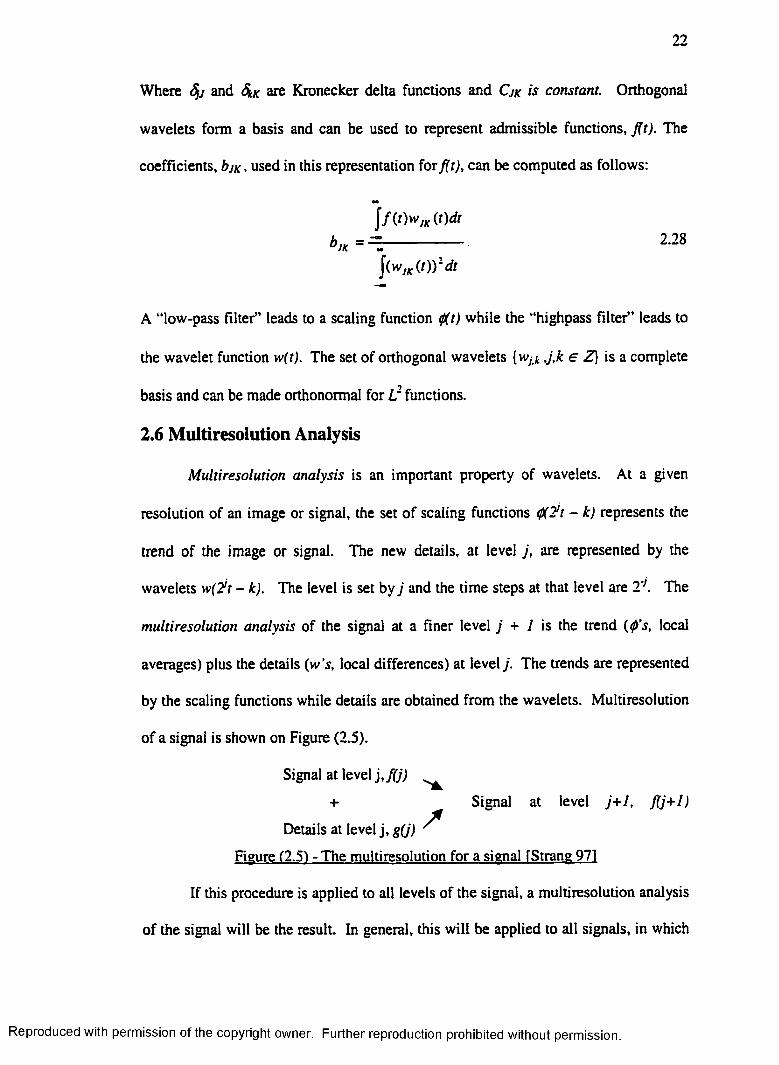
by the scaling functions while details are obtained from the wavelets. Multiresolution
of a signal is shown on Figure (2.5).
Signal at level ),f(j)
+ Signal at level j+1, fij+1)
Details at level j, g(j) ^
Figure (2.5) - The multiresolution for a signal fStrane 971
If this procedure is applied to all levels of the signal, a multiresolution analysis
of the signal will be the result. In general, this will be applied to all signals, in which
Reproduced with permission of the copyright owner. Further reproduction prohibited without permission.
23
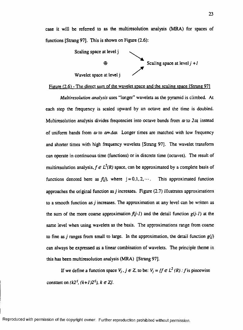
case it will be referred to as the multiresolution analysis (MRA) for spaces of
functions [Strang 97]. This is shown on Figure (2.6):
Scaling space at level j
Figure (2.6) - The direct sum of the wavelet space and the scaling space fStrane 971
Multiresolution analysis uses “longer” wavelets as the pyramid is climbed. At
each step the frequency is scaled upward by an octave and the time is doubled.
Multiresolution analysis divides frequencies into octave bands from (o to 2(0, instead
of uniform bands from oo to an-Act). Longer times are matched with low frequency
and shorter times with high frequency wavelets [Strang 97]. The wavelet transform
can operate in continuous time (functions) or in discrete time (octaves). The result of
multiresolution analysis, / e L2(R) space, can be approximated by a complete basis of
functions denoted here as flj), where j = 0,1,2,•••. This approximated function
approaches the original function as j increases. Figure (2.7) illustrates approximations
to a smooth function as j increases. The approximation at any level can be written as
the sum of the more coarse approximation flj-l) and the detail function g(j-l) at the
same level when using wavelets as the basis. The approximations range from coarse
to fine as j ranges from small to large. In the approximation, the detail function g(j)
can always be expressed as a linear combination of wavelets. The principle theme in
this has been multiresolution analysis (MRA) [Strang 97].
If we define a function space V j , j e Z , to be: Vj = ( f e Lr (R) : / i s piecewise
constant on (k2'j, (k+l)2'j), k e Z/.
© Scaling space at level j +1
Wavelet space at level j
Reproduced with permission of the copyright owner. Further reproduction prohibited without permission.

24
n
o
0 0 0 2 0 4 0 6 0 1 tJ) 0 0
M
O
Figure (2.7) - A function with approximations with increasing resolution of 1/2
Then as j increases, the sequence of spaces Vj(j €z) represents a ladder of subspaces of
increasing resolution. Since each subspace Vj consists of piecewise constant functions
over intervals of exactly twice the length of those for V;./. This sequence of subspaces
has the following properties:
1. ...cV .jC V l, c v ^ c v ; c V , c . . .
2- as j - > ~ 2 M
3- f e V , iff / ( i ) 6 V
4. / € V0 implies f i t - k ) e V 0 for all k s Z .
The third property means each space Vj is a scaled version of the original space Vo.
Each approximation can be written as the sum of a coarse approximation and a detail
function. If we define the best approximation of a function/in space Vj as P(j)f then:
P(jif=P(j-Df+g(j-lK 2.30
The detail function g(j-I) which is representative of the residual between two
approximations, can be written:
P i M = P U - l ) / + ! ( / . » ' , - u h - u • 231tez
Reproduced with permission of the copyright owner. Further reproduction prohibited without permission.

25
Where {wjtk , keZ} is a set of functions that are orthogonal to V, but not a complete
orthonormal system [Odgen 97]. The decomposition process can be done recursively:
The multiresolution analysis with wavelets is possible because there is a
sequence of 0 for j e Z that satisfies the properties (2.29) plus the following:
5. There exists a Reisz basis o f function 0 E Vq such that the set {0o.k = <t( t-k),
keZ} constitutes an orthogonal basis for Vo.
With property 5, the functions are wavelets (Wjk) such that (2.31) is always true.
In the case of the Haar example, we can chose 0(.t):
Where / represents the functions of the set [0,1). The function 0 is the scaling
function. The dilates and translates of the scaling function constitutes an orthonormal
basis for all Vj subspaces. These are simply scaled versions of V0.
2.7 The Wavelet Presentation
We conclude from the previous section that for any arbitrary scaling function
0, which creates a sequence of subspaces Vj that satisfy these five properties, a wavelet
function Wjrft) can be constructed such that (2.32) applies. To demonstrate this, using
the previous Haar example the Haar wavelet will be obtained. The following equation
will be used as the scaling function :
j -1
2.32l=7o *
2.33
0iMt) = 2!/20(2!t-k) 2.34
Reproduced with permission of the copyright owner. Further reproduction prohibited without permission.

26
where each Vj is the span of the set of functions { fa*, keZJ. The projection of an L2(R)
function, / , onto space Vj can be written as a linear combination of the dilated and
translated scaling functions:
« . /> / = 2.35t
The set {fat, keZ} is an orthonormal basis for Vj, thus, the scaling function
coefficients are computed:
m
= ( / . * « ) - [/(')*>„(')<*. 2.36
The mother wavelet w(t) can be determined using multiresolution analysis and a
scaling function 0(t), where 0 e Vo and also 0 e Vj. Since [0\x , k e Z} is a basis for
Vi, 0 c m be expressed as a linear combination of the 0ix's. For the Haar example this
is:
0(t) = ± 0 lo(t) + -j=0u (t) 2.37
The Haar wavelet associated with this scale function is:
W(r) = - L 0 io( t ) - - L 0 u (r). 2.38V 2 v2
From (2.32), the approximation o f /a t any resolution level j is composed of the
trend at the next lower level and the detail at that same lower level. The trend at level
j can be expressed as a linear combination of the scaling functions {0ix , k e ZJ. The
detail can be expressed as a linear combination of the wavelet functions (wj-i.k, k e Z}.
Since these Wjk functions are orthonormal, it is possible to define a space for which the
set of wavelets, with a single dilation index, forms an orthonormal basis :
Reproduced with permission of the copyright owner. Further reproduction prohibited without permission.

27
Wj = spanf\Vj.i k . k e Z}. 2.39
This produces the multiresolution property:
Vj = VH ® Wj.,. 2.40
The ® is used to represent the direct (orthogonal) sum of two subspaces. If the w,
subspaces are wavelets, they have property 3 (2.29) for the multiresolution analysis:
Equations (2.41) and (2.31) represent much of the formal value of wavelet analysis to
this research. Using these two equations, one can construct approximations with
increasing levels of resolution. These resolution levels are linear combinations of
dilations and translations of a scaling function <t>. The differences at each level of
these approximations are expressed in terms of linear combinations of dilations and
translations of a wavelet w. The relation between approximation (trend) and detail
spaces are shown in Figure (2.8).
Figure (2.8) - Relation between approximation and detail spaces
Two spaces R and S are said to be orthogonal, R±S, if every element of R is
orthogonal to every element of 5. With inter-space orthogonality, (2.40) extended:
fit) e Wj if and only i f fi2t) e Wj+i. 2.41
...
Vj = Vj.2 © Wj.2 © Wj.,. 2.42
Continuing for any arbitrary integer j:
V , = V ® @ W .J Jo / . . *
2.43
for j > jo\ for all j e Z, we have :
Reproduced with permission of the copyright owner. Further reproduction prohibited without permission.

28
2.44
hence
£/(/?) = ®W, .jez 12.45
The Haar example, in this context is shown on Figure (2.9) to illustrate the
approximation. Each approximation is written as a linear combination of the
appropriate basis functions The coefficients are found by taking the inner product
of/w ith the corresponding basis function:
c jjt = ( / ’ (x )dx- 2A 6
The scaling function coefficients and the wavelet coefficients provide information
about the function, similar to information provided by Fourier coefficients. The
difference being information in scaling or wavelet coefficients is more localized and
localization is controlled by the dilation index j.
3
3 O0•4 4 I 4PioiictnntorK
- * 4 0 2 4 4 0 2 4
Figure 2.9 - The Haar example function and its constant approximations
Reproduced with permission of the copyright owner. Further reproduction prohibited without permission.

CHAPTER 3
THE LIFTING SCHEME
3.1 Introduction
The development of lifting was inspired by the earlier work of Donoho
[Donoho 92] and Lounsbery et al [Lounsberry 97]. Donoho wanted to interpolate
wavelet transforms. Lounsbery et al. used a wavelet transforms of meshes that is
algebraically a special case of lifting [Sweldens 96a]. The Lifting scheme is an
efficient implementation of the wavelet transform. This scheme improved the
traditional wavelet transform and added several specific properties to it [Sweldens 95]
[Utterhoeven 97]. This scheme uses a simple relationship between multiresolution
analyses with the same scaling function. In the process the degrees of freedom are
isolated after fixing the biorthogonality relationship [Sweldens 96b]. Traditional
wavelets rely on Fourier analysis while the lifting scheme introduces wavelets without
using the concept of Fourier transforms. An important feature of lifting is that all
constructions are in the spatial domain. There are several advantages in working in
the spatial domain:
1) unlike the traditional wavelet transform, it does not require the mechanisms
of Fourier Transforms,
2) it leads to algorithms that can be generalized to complex geometrical
situations, and
3) it can be done by mapping integers to integers [Sweldens 96a].
29
Reproduced with permission of the copyright owner. Further reproduction prohibited without permission.

30
3.2 Lifting Operations (Split, Predict, and Update)
The wavelet transform of a signal is a multiresolution representation of that
signal [Strang 97]. Wavelets are functions that decorrelate the signal at each
resolution level [Daubechies 97]. The decorrelation of the signal at each level is
accomplished by splitting the frequency of the low pass part (trend) into a high and a
low-pass part at the next level. The lifting scheme is an efficient way to do this
process. In lifting the construction is entirely spatial and can be done without using
Fourier analysis [Sweldens 96a]. The following is an example that illustrates the
lifting method. For simplicity and convenience, we refer to this as lifting.
A Haar wavelet is the simplest and most convenient illustration of lifting.
Here, the steps in the Haar wavelet transform and lifting are summarized. The
integer version of the Haar transform will be referred to as the S transform
[Calderbank 96]. Suppose we have a signal (s = (s0l )teZ) with st e R . If the original
signal so.i has a length of 2", the discrete set representing the signal can be defined:
S = J„J ={s0j |0 < /< 2 - } . 3.1
Using the Haar wavelet, the average (trend) and the difference (detail) sequences can
be computed using the following relationships:
S j . 2 l + S j . 2 t + l j j 1 o
V l J = --------------2------------- d j - U = S J . 2 l + l - S i . 2 l ' 3 2
where, j denotes the level of decomposition and I =0,l,2,-- -,2"'7are the indices of the
elements in the signal. It is evident that with this transform, the signal is divided into
two disjoint “polyphase” components, i.e., the Sj.jj part with 2n'j'1 elements of discrete
pair averages and the dj.ij part with the same number of elements (+ one when total
Reproduced with permission of the copyright owner. Further reproduction prohibited without permission.

31
number of elements is odd) consisting of the pair difference. We use the notation in
[Daubechies 97] and refer to the even index elements as “evens” (se) and to the odd
indexed elements as “odds” ( S o ) . When the neighboring samples are highly correlated
the absolute value of the differences approach zero. This procedure can be applied to
the coarser part of the signal (trend) over and over until we exhaust all sample pairs.
Using Equation (3.2) one can reconstruct the original signal using the “odd” and
“even” sequences as follows:
Now, consider the Haar transform using lifting. First let’s address the auxiliary
memory locations. This process can be computed such that all needed computations
are done in-place. In lifting, the averages once computed, are stored in the even
sequence locations and the differences are stored in the odd sequence locations. Using
lifting, each difference is computed first and stored in the odd location. Then,
correspondingly the average is computed and stored, i.e.:
A computational procedure similar to this one for the Haar transform can be developed
and extended to more complex wavelets. In general for lifting, the original signal s is
split into two disjoint “polyphase” components, the “odds” and the “evens”. Due to
the existence of a correlation between “odds” and “evens” in the sequence s, one can
often construct a good predictor P to predict one from the other. This predictor is not
always exact and may necessitate adding a detail, d, to obtain an exact prediction,
where this detail is defined:
S j . 2 l ~ S j - U d ] - u / - a n d S j .2l+\ ~ S J - U + d j - u f ~ . 3.3
3.4
- n<1) S j - l . 2 l ~ S j .2l 3.5
Reproduced with permission of the copyright owner. Further reproduction prohibited without permission.

32
d = s , - P ( s 0). 3.6
The “evens” can be reconstructed once the detail d and the “odds” are obtained as:
se =P(s0)+ d . 3.7
The detail d is an approximate sparse set when P is a good predictor. This scheme
results in a lower first order entropy with d than that with So [Daubechies 97].
Perhaps the simplest predictor for an “odd” component is the average of its two
even neighbors:
= 3.8
Then the detail coefficients can be computed as:
d j - \ . k - S j . Z M ~ ( S j . 2 t + S /.2J+l ) ! - • 3 . 9
When the signal is locally linear, the average will be an exact prediction and the detail
will be zero. This process of prediction plus keeping the detail is lifting. Lifting
relates closely to wavelets, but wavelets require some separation in the frequency
domain. Lifting transforms (se,s0) to (se,d) which yield
poor quality frequency separation. This poor quality frequency separation is caused
by:
1) the aliasing produced as a result of subsampling se in the computations, and
2) inequality of the averages of the original samples s and the moving average
of se.
To correct this problem another lifting step is added [Daubechies 97] and [Calderbank
96]. The added step replaces the “evens” with smoother values (s) using an update
operator U defined as:
Reproduced with permission of the copyright owner. Further reproduction prohibited without permission.
33
s = sc +U (d). 3.10
Like prediction, this step is also invertible, i.e., se can be reconstructed from a given
(s,d) as:
se = s-U (d). 3.11
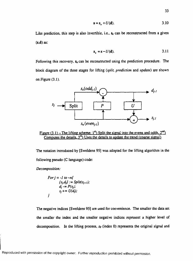
Following this recovery, s0 can be reconstructed using the prediction procedure. The
block diagram of the three stages for lifting (split, prediction and update) are shown
on Figure (3.1).
S p lit
Figure (3.1) - The lifting scheme: 1st) Split the signal into the evens and odds. 2nd) Computes the details. 3rd) Uses the details to update the trend (coarse signal)
The notation introduced by [Sweldens 95] was adopted for the lifting algorithm in the
following pseudo (C language) code:
Decomposition:
For j = -1 to -n{fsj,dj} := Split(sJ+i); dj -= P (Sj);Sj += U(dj);
}
The negative indices [Sweldens 95] are used for convenience. The smaller the data set
the smaller the index and the smaller negative indices represent a higher level of
decomposition. In the lifting process, so (index 0) represents the original signal and
Reproduced with permission of the copyright owner. Further reproduction prohibited without permission.

34
the s.j and dLi terms represent its two parts after the first splitting. In summary, the
forward lifting process can be written [Sweldens96a]:
• Split: The original signal is split into even indexed samples, spi, and the odd
index samples, Sjji+i. This splitting process is called the Lazy wavelet transform.
• Predict: The odd and even subsets are often highly correlated (if the signal has a
local correlation structure). Thus, it is possible to predict one from the other
d = se - P ( s 0). 3.12
• Update:
s = se + t/(d ). 3.13
The inverse transform operations are done by reversing the operations shown
on Figure (3.1), i.e., change the plus sign to minus and the minus to plus. The block
diagram of the three stages of the inverse lifting process (undo update, undo predict,
merge) are shown on Figure (3.2). A pseudo (C language) procedure for the inverse
lifting can be written:
Reconstruction:
For j = -n to - I f sj-= U(dj); d j + = P (Sj);
sj+i := Join(Sj,dj);}
In summary, the inverse lifting transform can be written [Sweldens 96a]:
• Undo update: Given d and se at each level one can recover the even samples at
the lower level by subtracting the update:
Reproduced with permission of the copyright owner. Further reproduction prohibited without permission.

35
s0 = s-U (d ) . 3.14
• Undo Predict: Given the even and the odd parts, one can reconstruct the odd
samples by adding the prediction:
d = s ,+ P (s 0) . 3.15
• Merge: Merge the even and odd samples to reconstruct the original signal:
M erge
Figure (3.2) - The inverse lifting scheme: 1st) undo the update, and recover the even samples. 2nd') add the prediction to the details and reconstruct the odd sample. 3rd)
merge to get the signal at the lower level
3.3 Building Other Wavelet Transforms
In the case of Haar transform, if the signal is constant the predictor is correct
and eliminates the 0th order correlation, i.e., the order of predictor is said to be one. If
the update operator preserves the average (the 0th order moment), then it is also
considered to have order one. In many cases, predictors that have higher order
moments are desirable.
A predictor of order two will be built. This predictor is exact when the original
signal is linear and the update preserves the average and the first moment. The
Reproduced with permission of the copyright owner. Further reproduction prohibited without permission.
36
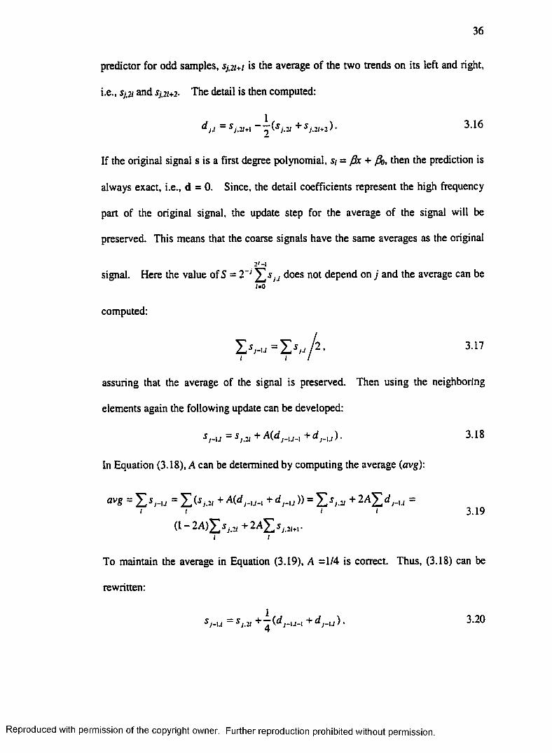
predictor for odd samples, s,.2/+/ is the average of the two trends on its left and right,
i.e., Sj'2i and s^m - The detail is then computed:
d j j = S j . 2 l +1 + S j . 2 l * Z ^ ’ ^ . 1 6
If the original signal s is a first degree polynomial, s i - fix ■¥ fio, then the prediction is
always exact, i.e., d = 0. Since, the detail coefficients represent the high frequency
part of the original signal, the update step for the average of the signal will be
preserved. This means that the coarse signals have the same averages as the original
2'-Isignal. Here the value ofS = 2 does not depend on j and the average can be
1=0
computed:
3 1 7/ / /
assuring that the average of the signal is preserved. Then using the neighboring
elements again the following update can be developed:
s h j = s , . v + M d J.u_l + dMJ). 3.18
In Equation (3.18), A can be determined by computing the average (avg):
^ 8 = Z s j- u = Z (sj.x + A(rf7-u-i + d j-u » = Z s d HJ =i i i i 3.19
(1 — 2A ) ^ Sj y + 2 A ^ Sj 2J+I. i i
To maintain the average in Equation (3.19), A =1/4 is correct. Thus, (3.18) can be
rewritten:
sj-u = sj.zi +~^(dj-|j_i +dj_u ) , 3.20
Reproduced with permission of the copyright owner. Further reproduction prohibited without permission.

37
and because of the symmetry in the update operator, we also preserve the first order
moment:
I ' ^ - U • 3 21i - i
The inverse can be done by computing the even and the odd components of the
original signal:
51.21 = s]-u +d j-u) 3.22
sj.ziH ~ d iJ +~^(sj.2! + 3.23
The lifting scheme for this example is shown on Figure (3.3).
- 1/2- i /2 - 1/2
> 1/4 + 1/4
Figure 3.3 - Illustration of lifting scheme for biorthoeonal Cohen-Daubechies- Feauveau (CDF 2.2) wavelet. Arrows marked ? are coming from/going to edges and
must be properly determined.
In this process, sometimes an element does not exist. For example, dj.u.i does
not physically exist at the left edge. Edges have not been discussed but will be in the
next chapter. A simple solution for treating the edges is to assume that the signal is
either periodic or infinite. The inverse of this lifting scheme (CDF(2,2)) can be easily
Reproduced with permission of the copyright owner. Further reproduction prohibited without permission.

38
done by simply reversing the arrows and changing the sign of the coefficients, on
Figure (3.3).
3.4 Polyphase Representations
The z-transform of a signal s is defined:
s(z) = X J 3.24
The z-transform of the subsampled s, i.e., v = ( i 2)s, is:
V(z) = -U (z 1/2) + s (-z ,/I)],and 2
the z-transform of the u = ( t 2 )(i 2)s is [Strang 97]:
U(z) = (T 2)V(z) = V ( z z) = U s ( z ) + s(-z) ) .
3.25
3.26
Subsampling a signal and keeping only the even “samples” yields se=fs2kf• The z-
transform of even “samples” is:
3-27
Similarly, the z-transform of the odd samples can be written:
*o(z) = Z ‘,S2*+l -* 3.28
5(0
Figure (3.4) - Splitting and reconstruction without Filtering fStrane 971
Reproduced with permission of the copyright owner. Further reproduction prohibited without permission.

39
Splitting and reconstruction in the z domain are shown on Figure (3.4). Note that the
(4 2)s(z) is exactly se(z).
The z-transform of the original signal s can be written in terms of these in the
following form [Strang 97] and [Daubechies 97]:
s(z) = se( z2) + z~ls0( z z). 3.29
Where, the se(z2) and s0(z2) are defined as:
, 2x [s(z) + s(-z)] J , [^(z) — 2)] , , nS ' i z ) = and s„(z ) = --------------- • 3.30
The z-transform of a finite impulse response (FIR) filter with filter coefficients /it can
be written:
Kz) = t i hkz ' k . 3.31*»*»
Where kt and h represent respectively the smallest and the largest k for which ft* is
non zero. The degree of Laurent polynomial h(z) is:
\h\=kt - k b, 3.32
which results in a filter length of \h\ + 1. Note that the degree of zero for the Laurent
polynomial is defined differently from that of the regular polynomial, in this case the
Laurent polynomial zf has a degree 0, while as a regular polynomial it would have
degree p. Here, we have set the Laurent polynomial of degree -<», to 0 [Daubechies
97].
A signal s filtered by h in the z-domain is:
q(z) = h(z)s(z). 3.33
The wavelet or subband transform of a signal s in z-domain is shown on Figure (3.5).
Reproduced with permission of the copyright owner. Further reproduction prohibited without permission.

40
© - >
H P
L P
Figure (3.5) - Discrete Wavelet Transform (DWT) in ^-domain IPaubechies 971
The forward transform uses the low-pass, h , and the high-pass, g , analysis filters
followed by subsampling. The inverse transform begins with upsampling and uses the
low-pass, h, and high-pass, g , synthesis filters. In general filters used for this purpose
are FIR. Thus, the conditions for perfect reconstruction is given by [Daubechies 97]:
h(z)h(z~l) + g(z)g(z~l) = 2, and 3.34
h(z)h(-z- ') + g (z )g (-z - ')= 0 . 3.35
The modulation matrix is defined:
M(z) =Kz) K -z ) gU) g(-z)
3.36
Using the modulation matrix the condition for perfect reconstruction can be written:
M (z '') r Af(z) = 2I. 3.37
Where I is the identity matrix. In the case of orthogonal wavelet transforms,
h - h ,g = g , and M (z) = M (z)is >/2 *1.
The polyphase representation of a filter h is:
h(z) = he(z2) + z-'hn(z2). 3.38
where, the subscripts e and o denote the even and odd elements respectively. These
elements are:
Reproduced with permission of the copyright owner. Further reproduction prohibited without permission.

41
he{z) = Y<h2kZk and A0(z) = ^ A 2t+Iz"*k k
This also can be written as:
The polyphase matrix then becomes:
P(z) =
This results in:
3.39
3.40
he(z) ge(z)
M z ) 8o(z)3.41
P(z z)t =^-M (z)1 z 1 - z
3.42
The polyphase representation of wavelet transforms is shown on Figure (3.6).
-►l - * c
P ( Z ~ 1) T P( z ) K
z z 1
Figure (3.6) - Polyphase representation of wavelet transform fDaubechies 971
The perfect reconstruction property can be expressed:
P(z)P(z~')T = 1 . 3.43
Where, both P(z) and P(z) contain only Laurent polynomials. This only possible if
the determinant of P(z) is monomial in z, i.e.,
|P(z)| = Cz', 3.44
where P(z) and P(z) are invertible matrices:
P (z)e G L(2;R[z,z‘])and P (z)e G L(2;R [z,z‘]). 3.45
Reproduced with permission of the copyright owner. Further reproduction prohibited without permission.
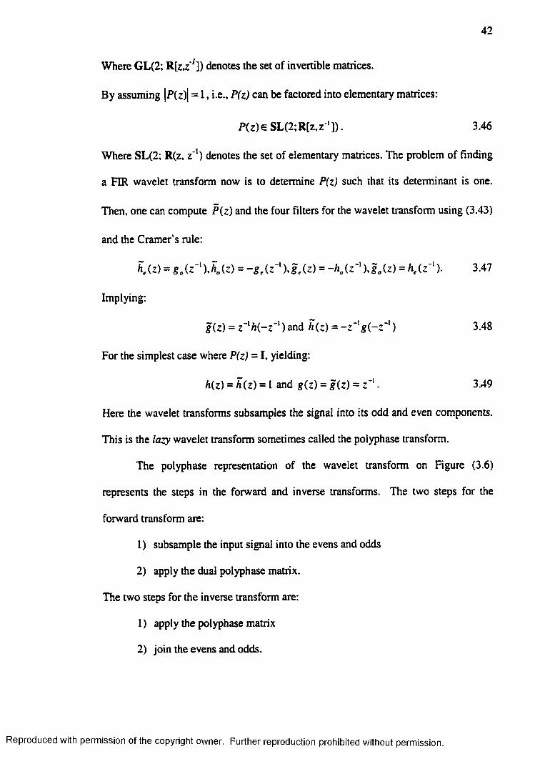
42
Where GL(2; R[z^'7]) denotes the set of invertible matrices.
By assuming |P(z)| = 1, i.e., P(z) can be factored into elementary matrices:
P(z)e SL(2;R[z,z1]). 3.46
Where SL(2; R(z, z '1) denotes the set of elementary matrices. The problem of finding
a FIR wavelet transform now is to determine P(z) such that its determinant is one.
Then, one can compute P(z) and the four filters for the wavelet transform using (3.43)
and the Cramer’s rule:
he (z) = g0 ( z '1 )Ji„ (z) = - g , ( z '1), g , (z) = -h a ( z - ), g„(z) = ht (z"‘ )• 3.47
Implying:
g(z) = z-lh ( -z -1) and h(z) = 3.48
For the simplest case where P(z) = I, yielding:
h(z) = h(z) = I and g(z) = g(z) = z‘‘ • 3.49
Here the wavelet transforms subsamples the signal into its odd and even components.
This is the lazy wavelet transform sometimes called the polyphase transform.
The polyphase representation of the wavelet transform on Figure (3.6)
represents the steps in the forward and inverse transforms. The two steps for the
forward transform are:
1) subsample the input signal into the evens and odds
2) apply the dual polyphase matrix.
The two steps for the inverse transform are:
1) apply the polyphase matrix
2) join the evens and odds.
Reproduced with permission of the copyright owner. Further reproduction prohibited without permission.

43
Definition 1. The synthesis filter pair (ft.g) is complementary when the determinant of
the polyphase matrix P(z) is 1. If (h,g) is complementary then the analysis filter
pair (ft, g) is also complementary. This will allow us to state the lifting scheme
[Daubechies 97].
Lifting uses complementary finite impulse response filter pairs (ft,g) to obtain a
new finite filter complementary to either g or ft. The new filter has some specific
properties [Daubechies 97]. Lifting is called primal lifting or dual lifting.
Theorem 1 (Primal lifting) : (ft,g) are complementary and another finite filter gnew
complementary to ft can be written:
The determinant of the new polyphase matrix does not change with this process.
Lifting relates ft and ft :
where s(z) is a Laurent polynomial and the dual polyphase matrix is given by:
g new(z) = g(z) + h(z)s(z2). 3.50
where s(z) is a Laurent polynomial [Daubechies 97].
Proof. The polyphase components of h(z)s(z2) are he(z)s(z) for even and for odd
hdz)s(z). After lifting the new polyphase matrix can be written:
3.51
h ntw(z) = h (z ) -g (z ) s ( z -1). 3.52
- 1 0 P ntw(z) = P M
UJ U - s l z " ) I3.53
Figure (3.7) shows the lifting scheme.
Reproduced with permission of the copyright owner. Further reproduction prohibited without permission.

44
h ( z-i - » Q — ► Q - » | h(z )
s(z)A A
(zA - Tm A
s(z) &-► HP © - ► g (z) l i
Figure (3.7) - The lifting Scheme: 1st) a classical subband filter scheme. 2nd) lifting the low-pass subband using the high-pass subband IDaubechies 971.
Theorem 2 (Dual lifting): If the finite filter pair (h,g) are complementary, then any
other finite filter hnew complementary to g can be written:
h™(z) = h(z) + g(z)t(z : ) , 3.54
where t(z) is a Laurent polynomial and after dual lifting the new polyphase matrix is
given by [Daubechies 97]:
P™(z) = P(z)1 0
t(z) I3.55
Dual lifting creates a new g :
g ntwU) = g ( z ) -h ( z ) t ( z -2) 3.56
The dual lifting is shown on Figure (3.8).
— r — <► l p j -*■ © - *
Kz) t(z)
K z )
&► © - * © — *-HP
Figure (3.81 - The dual lifting Scheme: Ist) a classical subband filter scheme, 2nd) lifting the high-pass subband using the low-pass subband IDaubechies 971.
Reproduced with permission of the copyright owner. Further reproduction prohibited without permission.

45
3.5 The Euclidean Algorithm
The Euclidean algorithm widely used to find the greatest common divisor
(gcd) of two natural numbers and can be extended to factor Laurent polynomials. The
gcd of two Laurent polynomials is defined up to a factor zp. Two Laurent polynomials
with a constant gcd are said to be relatively prime, i.e., p=0.
Theorem 3. Suppose we have two Laurent polynomials a(z) and b(z) * 0 where
| a(z) |>| b(z) | . Let adz) = a(z) and bo(z)=b(z), and iterate starting from i = 0:
ai+lU) = bi(z) and 6I+1(z) = al(z)mod(bl(z)) .
Then we can show that:
anC2> = gc:d(aCz).£>(z)),
3.57
3.58
where n is the smallest number for which b„(z) -0.
Proof. Since 161+1 (z) j<| bt (z) | , we can find a k such that | bt (z) |= 0 , thus the process
will end at an index value n - k + l . The number of steps in this process is bounded by
n <| b(z) | +1. If we define the quotient qi+i(z) = aizVbiz), then we can write:
an(z)0
As a result we can also write:
i=n 0 I T a ( l)
1 - ? , U ) I U ( z )3.59
o(z)b{z)
n=ni=i<ite) m K cz)
1 o o3.60
and a„(z) divides both a(z) and b(z). If an(z) is a monomial, then a(z) and b{z) are said
to be relatively prime [Daubechies 97].
Reproduced with permission of the copyright owner. Further reproduction prohibited without permission.

46
3.6 Factoring Complementary Filters (h,g) Into Lifting Steps
How are any pair of complementary filters (h,g) factored into lifting steps?
Here the Laurent polynomials he(z) and h0(z) have to be relatively prime, otherwise
any common factor would also divide the det(P(z)) because the det(P(z)) = 1. For any
complementary filter pair (h,g), it can be shown there always exists Laurent
polynomials s,[z] andr,[z] for 1 < i < k and a non-zero constant K>0 such that:
p w = n(=i
i s,(z) I i oT a: o 'o l I t ' U ) iJ[o 1 IKprimal dual scaling
3.61
Thus, every finite filter wavelet transform can be obtained by starting with the lazy
wavelet followed by k lifting and k dual lifting steps followed by a scaling. The
forward and inverse transforms are shown on Figures (3.9) and (3.10) respectively.
The dual polyphase matrix is [Daubechies 97]:
1 o' *1 ~t ' l / K o'- 5,(2'') 1 _0 1 0 Kp<->= n
i*i
In the orthogonal case {P(z) = P{z) ) we have 2 different factorizations.
3.62
LPl/K
HP
Figure (3.9) - The forward wavelet transform using lifting: lst~) lazy wavelet transform, then m primal and dual lifting steps, and at last scaling
Reproduced with permission of the copyright owner. Further reproduction prohibited without permission.

47
L P
uz) r ~ t,iz) —l— X Sm(z) l— = — J/(z)
^ T j)>
Figure (3.101 - The inverse wavelet transform using lifting: 1st) scaling, then the alternating m dual and primal lifting steps, and last the meree (inverse lazy transform)
Computing the wavelet transform using lifting is done in several stages. In general, m
primal and dual lifting steps follow the lazy wavelet transform. The lazy transform
splits the signal into its even and odd indexed components: s0l =s0 2l and d0l =s0 2lH .
A dual lifting applies a filter to the even components and subtracts the result from the
odd components:
3.63
and the primal lifting does the opposite, i.e., applies a filter to the odd components and
subtracts the result from the even components:
SJ J = S H J - ' Z Ui.kS,.t-k- 3-Wt
These (after m pairs of primal and dual lifting steps) become the low-pass and the
high-pass coefficients respectively up to a scaling factor K:
smJ = smJIK and dml = Kdml. 3.65
The inverse transforms are obtained by reversing the operations and flipping the signs
[Calderbank 97]. The forward and the inverse transforms are shown on Figures (3.9)
and (3.10) respectively.
Reproduced with permission of the copyright owner. Further reproduction prohibited without permission.

48
3.7 Haar Wavelets
The z-transform of the filter coefficients for the Haar wavelets are:
, - ih(z) = l + z~
g(z) = - l /2 + l/2 z’1
h(z) = 1/2 + 1/2 z' 1
g(z) = - l + z' 1
These are not normalized. Using the Euclidean algorithm, the polyphase matrix:
3.66
'1 - 1/ 2' ri o iri - 1/ 2'_! 1/2 ; d c 1
3.68
P (z)= " 7 . " = ' ' II : " “ , 3.67
is obtained and the resultant inverse is:
. - f 1 1/ 2II 1 0- w < ) - [ 0 , JL_l ,
The original signal is [sQJ}. The forward transforms for these are:
s-u = so.n
d-ij = O.a+t
djj = d,-u ~ Sj-\j
s j j = 5 j - u + 0 ’ t 2 ) d j - u
where j represents the level of decomposition and I represents the elements. The
inverse for (3.69) becomes, respectively:
3.69
s j + u ~ s j j
dj+U — dji + Sjj3.70
•Viz+i — d-u
S 0 .21 ~ S - U *
where the inverse process begins from j = m the maximum level of decomposition
[Uytterhoeven 97] and [Calderbank 97].
Reproduced with permission of the copyright owner. Further reproduction prohibited without permission.

3.71
49
3.8 Biorthogonal Cohen-Daubechies-Feauveau Wavelets
The biorthogonal Cohen-Daubechies-Feauveou (CDF) wavelets are denoted
with (N , N ) , where N and N represent the number of vanishing moments for the high
pass synthesis filter g and the high-pas* analysis filter g respectively. The following
examples are taken from [Uytterhoeven 97] and [Calderbank 97].
3.8.1 CDF(l,x)
g(l,x): (l,-l)v i
h (1,1): - ( 1,1)
£(1,3) ^ ( - l , 1,8,8,1,-1)16yfl
h (1,5): — (3-3-22,22,128,128,22-22-3,3).256
Using the factoring algorithm, the lifting steps are:
djj = djj ~ su
CDF(1,1) : Sjj = S j j+ ~ d /A
CDF(1,3): Sjj = Sjj " - %d ji + d /tU)
C D F (U ):s ,J = s iJ - 2 d,_u - 1 2 8 + 2 2 d ,.u - 3 d „ u )
The normalization factors for the CDF(l,x) are: nL = yfl and nH = - J l / l .
3.8.2 CDF( 2,x)
|( 2 , x): ^ ( 1 - 2 ,1 )
S(2,2, 4 ( - U 6.2,- l ,o
3.72
Reproduced with permission of the copyright owner. Further reproduction prohibited without permission.

50
sft (2,4): —— (3,-6-16,38,90,38,-16,-6,3)
128P)
ft (2,6): — (-5,1034 -78,-123,324,700,324,-123 -7834,10,-5) 1024
V2ft (3,1): —— (-133,-1)
4
ft (3,3): — (3-9-7 ,45 ,45 ,-7 ,-93)64Pi
ft (3,5):— (-5,15,19,-97,-26,350,350,-26,-97,19,15,-5). 512
The lifting steps are:
1 ,
■*;./ “ ^ >~U
CDF (3,1): +—djU
3.73
The lifting steps are:
djj = djj + sj+u)
C D F(2,2):^J - s l l - ^ ( - d M J- d , J)
C D F (2 A )sll = s„ — O dr -u -1M ^.U - t9 r fw + 3</„u ) 3.740 4
C D F ( 2 ,6 ) : s , j - s , , - j ^ { - 5 d I_u +29d,.,J - i6 2 d lAJ -162d tJ *
39d]+u ~5d ;+:j).
The normalization factors for the CDF(2,x) is, nL =-Jl and nH = V2 /2 .
3.8.3 CDF( 3,x)
V2|(3 ,x ) : -(-1 ,3 ,-3 ,1)8
3.75
Reproduced with permission of the copyright owner. Further reproduction prohibited without permission.

51
CDF(3,3): s „ = s ;J - ^ ( - 3 4 ,_ „ -1 6 4 ,, + 34,.,,)36 3.76
CDF(3,5)-.J„ = s „ * 34d,-.J - 128rf,J +34<i,.u
For this case the normalization factors are: nL = 3V2/2 and nH = V2 /3 .
3.8.4 CDF(4,x)
g (4 ,x ) : ^ - ( - 1 ,4 - 6 ,4 - 1 )16
£(4,2): — (3,-12,5,40,5,-12,3)32J 2
£(4,4): -(-10 ,40 ,-2 ,-192,140,560,140,-192,-2 ,40 ,-10) 3.77512
£(4,6): -— -(35,-140,-55,920,-557,-2932.2625,8400,2625,-2932,8192
-557,920,-55,-140,35).
The lifting steps are:
s jj = sjj +dj.t)
d jj ~ d ,j ~ ( sjj +5/+ij)
CDF(4,2) )16 3.78
CDF(4,4): = s„ - - 2 ^ ,- u - 294,, + « , . u )
CDF(4,6): j „ = j „ - ( - 3 5 4 , . , , + 2654,.,, -9984 ,.,, -9984 ,, +
2654,.,, -3 5 4 ,.,,) .
The normalization factors are: nL = 2-Jl and nH = V2 /4 .
3.8.5 CDF(5,x)
J 2g (5 ,x ) :^ - ( l , -5,10,-10,5,-1)
32
Reproduced with permission of the copyright owner. Further reproduction prohibited without permission.

52
ft (5,1) :■^(3,-15,20,20 -15,3)16R
ft (5,3): -^(-5,25,-26,-70,140,140,-70,-26,25,-5) 3
v ?ft (5,5): - (35,-175,120,800,-1357,-1575,4200,4200,
4096-1575,-1357,800,120,-175,35).
The lifting steps are:
^ = ^ - ^ ( 1 5 ^ + 5 ^ )
di! = d ;J - — (15i;J +9s;, u )
C D F W - . ^ j ^ s ^ + ^ d ' j 3.80
CDF(SJ ) : slU = s ;J - ( -5 < * ,-u " + 5<i„u )
CDF(5,5) = = J ,, - ^ j ( 3 5 ^ -2 3 0 d ,.u -7 6 M ,, +
230^,.,, -35</Jt;J).
The normalization factors are: nL = 3-^2 and nH = V2/6 .
3.8.6 CDF(6,x)
V2g (6 ,x ): -^(1,-6,15,-2045,-6,1)64
V I/i (6,2): — (-5,30,-56,-14,154,-14,-56,30,-5)64J ?
ft (6,4): - — -(35,-210,330,470,-1827,252,3948,252,-1827,2048
470,330,-210,35)
ft (6,6): —— — (-63378,-476,-1554,4404,1114,-13860,4158, . c .16384 4.81
28182,4158,-138604114,4404,-1554,-476,378,-63).
Reproduced with permission of the copyright owner. Further reproduction prohibited without permission.

53
The lifting steps are:
d j j = d j j
S,J = S,j ~ ^ 9dn<J + M ,j)
* ,l = d ,i + 4s ,.u>
CDF( 6 , 2 ) : = s tJ ~ ( - H fU - 5 d ;J) 3.82
CDF(6,4): j„ , = s tJ - 195</,.u - 19M,, + 3M ,.U)
CDF(.6,6) : SjJ = «w ~ + 4 6 9 ^ -1686</,.U -
1686djj +469d;tU -6 3 d JtU).
The normalization factors for this case are: nL = 4-Jl and nH = V2 /8 .
3.8.7 CDF(2+2,2)
This wavelet is built with one extra lifting step forming a new transform with 4
vanishing moments in the high pass analyzing filter using CDF(2,2). This transform
was inspired by the Split (S) plus Prediction (P) transform known as the S+P
transform. Since the new transform is not the same as CDF(4,2) it is denoted
CDF(2+2,2). The lifting steps for this transform are:
d , j - d j j + s j +\ j )
s iu ~ sjj +~(d j-u 3 83
d , j ~ a ( ~ ~ ^ s i - u + s j . i ~ ~ ^ s j + u ) + + s j * u ~ ~ ^ s j + i j ) +
tfj+u
To obtain 4 vanishing moments:
S/3 + 3y = l 4a + 4 0 + y = l.
3.84
Reproduced with permission of the copyright owner. Further reproduction prohibited without permission.

54
Some possible values [Calderbank 98] [Calderbank 96] are:
(a) ar = 7 ’^ = 0>J' = To J
(b) a = , /8 = , r = 0 3.85o o
(c) a = j , / J = ~ , y = l4 4
3.8.8 Symmetric Biorthogonal Transform (9-7)
The symmetric biorthogonal transform (9-7) is very popular and was used by
[Birslawn 95],[BirsIawn 96],[Bradley 96] for FBI finger print compression. The high-
pass filter has 7 coefficients and low-pass filter has 9 coefficients. Both the analysis
and synthesis high pass filters have 4 vanishing moments. The lifting factorization
steps for the input transform are:
Step( 1):
d a = dtj + (x{ Sj j + sj+2j )
S j j = s , j + 0 V i j + d HJ ) 3g6
Step(2):
d jj = + /(Sjj + Sj+U)
s,j = s1u+ #(d j j + d,-u)-
W herea = -1.586,^ =-0.053,y = 0.883,(5’= 0.444and the normalization factor K =
1.149604398.
3.8.9 D4
Finally the orthogonal transform, Daubechies 4 (D4). The lifting steps for this
are:
Step( 1):
d jji ~ d jj ~ )
Reproduced with permission of the copyright owner. Further reproduction prohibited without permission.

55
Step( 2):
s tj = s » +(:j d i j+ ^ r ' ‘l ‘-u ) 3-87
dj j - dj j + s j+u
The normalization factor for D4 is: K = >/3 + l/>/2 = 1.577.
It should be noted that in these examples, no rounding was used. In general,
the terms in the brackets are rounded to an integer. In this dissertation, the values that
appear in the parenthesis in the above equations are rounded to the closest integer by
adding 1/2 to the bracket term and then truncating the result to this integer.
3.9 Two-dimensional Lifting
The most common approach for lifting in 2 dimensions is to lift the rows then
columns. This will produce 4 subbands similar to those obtained by a 2D wavelet
transform. It is essential that the normalization factor be properly determined for the
process. At each level of decomposition 4 subbands, LL, HL, LH, HH, are obtained
and the normalization factor must be computed for the subband being computed. The
general normalization factor AT has the following pans [Uytterhoeven 97]:
Kll - riiJiu Kut = nL.riH, Khl - nH-nb and Khh — »»•«//•
In the next chapter new methods for 2-D lifting of a 2-D image will be
presented.
Reproduced with permission of the copyright owner. Further reproduction prohibited without permission.

CHAPTER 4
IN-PLACE COMPUTATION OF LIFTING AND A NEW SINGLE AND SET IMAGE SCANNING METHOD
4.1 Introduction
In this chapter the treatment of images will be discussed. We will also
demonstrate in-place calculations with the order of assignment of the indexes of a 1-D
array to properly store the pixels of a 2-D image, and perform the lifting steps. The
treatment of the edges introduces several techniques developed in this research that
scan the image as a 1-D array in a specified format. These new scanning methods
reduce the number of edges and improve their treatment.
4.2 The In-place Calculation for Lifting
The in-place calculation for lifting a 2-D image requires careful arrangement of
the indexes of the 1-D signal that represents the 2-D image. Each element array
representing the image in the pixel domain or transformed domain is denoted as sJJC.
Where, j denotes the lifting step and k the element in the array. For a signal of size
2n, j and k have the following values:
-1 > j> - n and 0 < k < 2"*1. 4.1
Note that the index j representing lifting steps is a negative number which simplifies
the implementation. The array used at each lifting step for the trends is s and the
details is d. The trends and the details after the first split are: = s0 2iand
du = s0 Zk+l, with k from 0 to 2n+J. For illustration, an array of 8 elements is used as
' 56
Reproduced with permission of the copyright owner. Further reproduction prohibited without permission.

57
the original signal, s = {Sjk|y = 0, 0 < k < l }. One may think of this as a column or a
row of an 8x8 pixel image.
The CDF(2,2) is the Cohen-Daubechies-Feauveou biorthogonal wavelet with 2
vanishing moments for the high-pass synthesis filter (g) and 2 vanishing moments for
the high-pass analysis filter (g) [Uytterhoeven 97][Calderbank 97]. We begin with
the Haar lifting steps with rounding:
Where, j_ J denotes adding — inside the brackets of the detail and the trend for
CDF(2,2) in (3.60) then truncating to an integer. To compute (4.2) and (4.3) in-place,
we write the steps using s, the original signal. Table (4-1) demonstrates the in-place
lifting for the CDF(2,2) wavelet with array s. The following is the in-place calculation
process for trends and details:
(4.4) represents the details and (4.5) represents the trends. In lifting the details (4.4)
are computed first, then the trends. The lifting steps for CDF(2,2) will be illustrated
with the sample signal s.
4.2.1 The CDF(2,2) Lifting
4.2
sj.t ~ + ^ (4j.k-i + d jJc) + ^ 4.3
s[2_;"‘ +2*' *Jfc]=42' ' ' 1 + 2 ~J * * ] - |( s [ 2 - ' *k] + s[2'1 + 2 '1 * k ]) 4.4
j[2' ; */t] = j[2*; */t] + - ( 5[2' y * k - 2 - J-i] + s[2'1 *k + 2 'J~1])4
4.5
Reproduced with permission of the copyright owner. Further reproduction prohibited without permission.
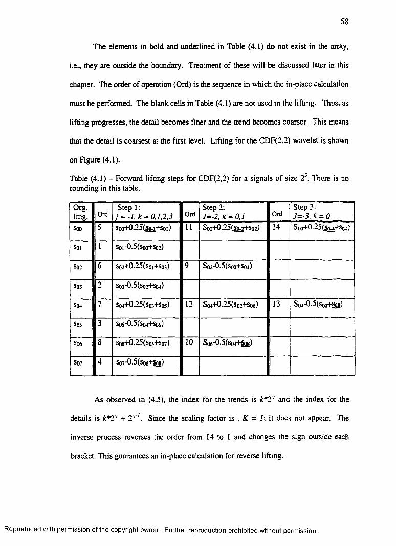
58
The elements in bold and underlined in Table (4.1) do not exist in the array,
i.e., they are outside the boundary. Treatment of these will be discussed later in this
chapter. The order of operation (Ord) is the sequence in which the in-place calculation
must be performed. The blank cells in Table (4.1) are not used in the lifting. Thus, as
lifting progresses, the detail becomes finer and the trend becomes coarser. This means
that the detail is coarsest at the first level. Lifting for the CDF(2,2) wavelet is shown
on Figure (4.1).
Table (4.1) - Forward lifting steps for CDF(2,2) for a signals of size 2J. There is no rounding in this table.
Org.Img. Ord
Step I:j = - l .k = 0,1,2,3 Ord
Step 2:J--2, k = 0,1 Ord
Step 3: J=-3. k = 0
Soo 5 Sqo+ 0 .2 5 (S o. i + sqi) 11 S qo+ 0 .2 5 (S q.2+So2) 14 S qo+ 0 .25(S (m ~<-S(u )
Soi 1 So|-0 .5 (S oo+S02)
S02 6 S02+0,25(Soi+So3) 9 S o2*0.5(Soo+So4)
S03 2 So3*0.5(So2+S{)4)
S04 7 So4 + 0 .2 5 (so3+Sos) 12 S o4+ 0 .25 (S o2+S<)6) 13 S o4-0.5(S qo+Sjj8)
So5 3 So5-0.5(So4+So6)
S06 8 So6 + 0 .2 5 (S os+S07) 10 So6-0.5(so4+Sgg)
S07 4 Sq7-0.5(S06+Sqs)
As observed in (4.5), the index for the trends is k*2'J and the index for the
details is k*l'J + 2'J‘/. Since the scaling factor is , K = /; it does not appear. The
inverse process reverses the order from 14 to I and changes the sign outside each
bracket. This guarantees an in-place calculation for reverse lifting.
Reproduced with permission of the copyright owner. Further reproduction prohibited without permission.

59
In this demonstration of lifting, we used an array of 8 elements. For an image
with an array of 256x256 pixels, there are 256 rows and 256 rows. The most common
method of lifting for a 2-D image is to lift the rows then the columns [Daubechies 97].
Several scanning techniques that decorrelate the image so that it can be viewed as a 1-
D signal will be presented later. The in-place lifting computation for several other
wavelets have also been obtained. These lifting steps are implemented in C.
Original:
(So) © © ) (© © ) (© (© (©Step 1:
*c.................
.W ldia) (S) v W U h
K .
vS06/l Vd 13> A'’-A A ^ ^ hr Ar
(© (© © ) ( © Q (© (©
Step 2:I---------
( © © ) © )^ J © )
' * © © © © © © © ©
Figure (4.11 - Illustration of lifting for the CDF(2.2) wavelet on an arrayof 8 elements. Dashed arrows need additional consideration.
Reproduced with permission of the copyright owner. Further reproduction prohibited without permission.

60
43 A New Single Image and Set Image Scanning Method
The pixels at the edges of the signals (rows and columns of a 2-D image) must
be treated differently than the internal pixels. To fix this edge problem, an image or
signal is often assumed to be either periodic or infinite [Sweldens 96b]. Assuming a
periodic image means that the pixels at one edge of the image are assumed to be
followed by the pixels at the other edge. This can be imagined as the image being on a
cylinder. Thus, lifting often uses values from one edge of the signal for the
“boundary” pixels at the opposite edge. In medical images, the edges (left, right, top,
and bottom) are usually the background which surrounds the diagnostic part(s) of
medical interest and adopts well to either periodic or infinite “image” treatment.
In the infinite image method, the edges may be treated in two different ways:
1) Assume that the image continues with the same intensity as the last or first♦
pixel depending on the edge of the signal that is being considered, or
2) Assume the same rate of change for the points before or after the first and
the last pixels respectively. In either case the method works well due to the
presence of the background.
In some cases the elements before the beginning and after the end of the signal are set
to zero. Regardless of the method used, a prefect reconstruction is possible only if the
treatment of the “edges” produce exactly the same signal in the reconstruction as the
original signal.
Although techniques may result in perfect reconstruction, they may result in
different values at the edges. When one studies an the image in an transformed
domain (wavelet and lifting domains), the accuracy of edge treatment is very
Reproduced with permission of the copyright owner. Further reproduction prohibited without permission.

61
important. An incorrect representation of the edges is misleading. For example,
suppose the pixel value on an edge is 200 and the pseudo point outside the edge is
zero. The average of these two points is 100 with the Haar transform. This procedure
in reconstruction obtains the exact pixel value. However, when we use different
values to represent the pseudo pixels outside the boundaries, the results are different in
the transformed domain. In the previous example, if instead of zero 200 is used for
the pseudo pixel the average is 200. In the transformed domain the same pixel has 2
different values that depend on the pseudo pixel.
The edge problem is more pronounced with multiple edges, e.g., 2-D medical
images where lifting is usually performed rows followed by columns [Calderbank 96].
In this case each row or column is treated as a signal with two edges (ends).
Depending on the lifting for an M*N image, it has M rows and N columns, or 2* M*N
edges. The treatment of edges has even more effect on transforms when an entire set
of similar images is being transformed. In the following sections several new
scanning techniques for 2-D single images and a set of images are presented. These
new techniques reduce the number of edges and improve transformed results.
4.3.1 Boundary Value Estimation
There are several common methods to handle signal boundaries. The following is the
summary of different methods commonly used:
1) Boundary Value Padding Method (BVPM):
In this method, the pixel at the boundary is used for pixels before or after the
boundary. That is:
A.j = Ao and Am*n = Am*/v-/,
Reproduced with permission of the copyright owner. Further reproduction prohibited without permission.

62
where j = 1,2,—k represents the index of pixels located before (pixel 0) or after (pixel
M-l). This method is shown on Figure (4.2).
Pixel Value
M M +l Pixel No.
edgeM -l
Figure (4.2) - The Boundary Value Padding Method (BVPM)
2) Reflective Boundary Method (RBM):
In this method, pixels outside the boundary are assumed to be a reflection of the pixels
in the image. Figure (4.3) illustrates the reflective boundary method.
Pixel Value
■ €(> #
M M+l Pixel No.edgeM-l
edge(boundary)
... .. * A m *N-3 A m *N-2 A m *N-I 1 A m *N-I A m *N-2 A m *N-3 ... ...
Figure (4.3) - Illustration of the Reflective Boundary Method
This is:
Reproduced with permission of the copyright owner. Further reproduction prohibited without permission.

63
A.j = Aj and Am*n+j — Am'n-^
where j = l,...k represents the pixels being reflected.
3) Symmetric Extension Boundary Method (SEBM):
This method extends the images in a continuous way at the boundaries [Strang
97]. Usually, an extrapolation technique predicts the values of the pixels outside the
boundary using the points in the boundary. The extrapolation technique may vary
depending on the pixel values in the image next to the boundary (edge). This method
is shown on Figure (4.4). The values for pixel M and M+l were obtained by
extrapolation.
Pixel Value
J
edge M M+l Pixel No.M-l
Figure (4.41 - Illustration of the Symmetric Extension Boundary Method (SEBM)
4) Zero Padding Method (ZPM):
The pixels outside the boundary are set to zero. This method often results in a
sharp jump at the boundary (edge) when the pixel value at the boundary (edge) is not
zero [Strang 97]. In grayscale medical images with black backgrounds, the ZPM is
suitable. This method is widely used in wavelet decomposition of a signal to extend
the signal when its length is not divisible by the length of the filter. MATLAB
supports this method [Misiti 97].
Reproduced with permission of the copyright owner. Further reproduction prohibited without permission.

64
4) Wrap-around Boundary Method (WBM):
This method is also referred to as circular convolution [Strang 97]. Using this
method one can view the image as being on a cylinder. Thus, the values from one
edge of the signal are used for the pixels outside the boundary at the opposite edge.
This method also works very well with the grayscale medical images that have a
continuous background. This method is shown on Figure (4.5).
same edge
Am»n-i I Ap Am-N-2 Am»N-| t Ap...A1
Figure (4.5) - Illustration of the Wrap-around Boundary Method (WBM)
Using this method, the edges of the signal merge. This method is widely used in
wavelet decomposition when the number of data points is not divisible by the number
of filter coefficients [Press 96].
4.3.2 Spiral Scanning*
%
Spiral scanning scans the continuous-background of each image of the set as a
“rectangular spiral.” The continuous-background is made up of all the pixels in a
single pixel width path around the image with values less than a predetermined
threshold. The determination of the continuous-background with a “rectangle spiral”
is referred to as background isolation. In medical grayscale images the background
pixel intensities are almost always nearly zero. Therefore, the lifting scheme is only
applied to the foreground of each image in the set. Each image’s foreground isn
considered to be 1-ESfor processing. As shown on Figure (4.6), background isolation
starts with the pixel located at the upper-left-hand comer of each image and is
Reproduced with permission of the copyright owner. Further reproduction prohibited without permission.

65
processed as a rectangular spiral, pixel by pixel, until the threshold is exceeded (Figure
(4.9), top row). The threshold was determined statistically using different values to
isolate:
1) the background of each image that surrounds its diagnostic foreground, and
2) any “padded” background that is added to make the image a specified size
(256x256 in our case).
The “padded” and digitized background pixels are very close to zero, but not zero. A
threshold of 50 was determined to be appropriate for both backgrounds. The address
of the pixel where the threshold is exceeded is saved in a Tag array. There is one
entry in the Tag array for each image in the set. The N*M -TagfimJ remaining pixels
of each image, im, are also scanned as a rectangular spiral and added into array, b. The
scanning proceeds from image to image until all images in the set are processed. An
example of this scanning technique is shown on Figure (4.7).
Ao • ----
A, a 2 An-2 An-1
An An+i An+2 . . . . . . A2N-2 A2N-1
Ain
— ? ►A3N-1
. . . . . .
. . . . . .
A(M-2)N A (M-l)N-t
A(M-i)N A(M-t)N+l A(M-l)N+2 . . . . . . AmN-2 ^MN-I
Figure (4.61 - Spiral scanning of a single image
Reproduced with permission of the copyright owner. Further reproduction prohibited without permission.

66
in [i [<i11
K H IB ! 23 56
14
14
i i B S E S K a i a -
i1) is i ; u, ss 4
1 4
is41 4
background
Data
1( a ) - T ;st image CK)V
11_______ 1i- ’L8— -15— U . . . _5L_____ _J3__ - 4 \
n~3~ 8 9 23 56 121 i61 B~5~ 23! 56 _87 __129 C231 y i~0~ “
16!1 67 8 ty 1*40i >
' \ 2i& |» i
~T~ 6 ; 57 j 45J
n 1 1 <2 /1 8 !
_17!.. 19 J L . 16 J ii 9 ! 1
2 “5 17 A 5 3 8 9/»— i
19 |
( b ) - Test image (2) /
4 14
5 1
m 9 23
23 56 87
” 16“
67 [ 1 80 „
~b~_
57 j 45
~TF “ 19 18
i ; ii 4 12
saE 9 B S 1 K 9 |s
u r a n■ B ilB B ilM f i<>
E I U Q -g a a a a 11
4 S 4 14
background
^ s
Data
background
Data
(c ) -T e s t image (3)Figure (4.7) - An example of spiral scanning technique
Reproduced with permission of the copyright owner. Further reproduction prohibited without permission.

67
The pseudo code for spiral scanning method is:
Begin: j - 0 ;Loop over images, im, 0<im< nimages.
Re-write the current 2-D image in a clockwise rectangle spiral format in a 1-D array
A [].Start from the first pixel, A[0], read pixels A[i] until A[i] > threshold i = 0;
whilefAfi] < threshold){
i++:}Taglim] = i;Add the pixels from Tag[im] after the last pixel in the 1-D array b[]: whilefi < number o f pixels in image im)f
b[j++]=a[i++];}End loopLift the 1-D array b[]Apply to £>[] lossless compression: Huffman, LZ, LZW, ...Include image size sequence, nm[0] nm[l] ... nm[nimage-l], and image Tag sequence, Tag[0] Tag[lJ ... Tag[nimage-1], in compressed data
End.
The foreground spiral scanning is presented in the middle row on Figure (4.9).
The spiral scanning always proceeds clockwise for both the background isolation and
the lifting.
In an effort to improve scanning and isolate the image background better,
several modifications of spiral scanning will be presented next.
The difference for the first modification of the spiral scanning presented is in
the foreground scanning as it proceeds from image to image. Previously, the
foreground scanning proceeded from the center pixel of one image to the tag pixel of
the next image in the set. Here it proceeds from image to image starting at the
location of the last pixel scanned in the previous image. So, if scanning ended at the
Reproduced with permission of the copyright owner. Further reproduction prohibited without permission.

68
center of the image doing a clockwise rectangle spiral, it begins at the center of the
next image and does a counter clockwise rectangular spiral terminating at the tag pixel
of the next image. An example of this technique is presented on Figure (4.8).
s is Id o I i 14 r
EHBHSSSSHH / ] t a i E a ^ i i a
>) i:
i: is4 / r i o i s i ; u> s o
: / s is i: S 0 l ‘»
( a ) - t ? s t image (1)
B
( b ) - Test image (2) /
10 14 10 IS 11 0
s IS 10 0
EHBiPliPIBSliBm m iiBBina■ B m a i a i a i a
S 17 17 S 0 l 1)
background
data
background
data
background
\\I
/
data
( c ) - Test image (3)
Figure (4.8’) - An example of modified spiral scanning technique
Reproduced with permission of the copyright owner. Further reproduction prohibited without permission.

69
This new technique is shown on Figure (4.9) below the original spiral scan for
comparison.
*
Taglf)/ Tagl i ft
f Tag[2] Tag[31 1
Spiral Background Isolation Method (SBIM), setting Tags
♦
The Image Set Spiral Scanning Method
, [ » &
The Enhanced Image Set Spiral Scanning Method
Figure (4.9) - Illustration of the spiral scannine method and the modified scanningmethod for a medical image set.
The pseudo code for the enhanced spiral scanning method is:
Begin: j = 0;Loop over images, im, 0 < im < nimagesRe-write the current 2-D image in a clockwise spiral format in a 1-D array
A[J.Start from the first pixel, A[0], read pixels A[i] until A[i] > threshold:
i = 0;while(A[i] < threshold){
/++,*}Tag[im] = i; ifim is odd){
Add the pixels from Tag[im] after the last pixel in the 1-D array b[J: while(i < number o f pixels in image im)I
b[j++)=a[i++J;}
Reproduced with permission of the copyright owner. Further reproduction prohibited without permission.

70
else{Add the pixels from the last to Tag[im] to the b[J: i = npixels; while(i > Tagfim]){
b[j++]=a[i~];}
}End loopLift the 1-D array b[]Apply to b[] lossless compression Huffman, LZ, LZW, ...Include nimages, image size sequence, nm[0] nm[l] ... nm[nimage-l], andimage Tag sequence, Tag[0J Tag[l] ... Tag[nimage-1], in compressed data
End.
Two more modifications were studied because the background is frequently
not evenly distributed around the diagnostic foreground of an image. Because of this,
a rectangular spiral may not be the best to isolate the background. The difference
between these two modifications is that one initiates scanning from the sides (Figure
4.10) and the other from the top/bottom of image (Figure 4.12).
In the first of these two, scanning the background was done on both sides of
each image in an up-down manner and is referred to as vertical isolation. Vertical
isolation determines two pixel addresses where the threshold is exceeded on the left
and the right side of an image. These addresses are stored in Tagl[im] on the left and
Tag2[im] on the right. The vertical background isolation process is presented on
Figure (4.11). The pixels between Tagl[im] and Tag2[im] are vertically scanned and
added to the 1-D array b used for lifting after the scanning.
The second initiates its scanning at the top of the image in a left to right
manner until the threshold is exceeded. This pixel address is Tagl[imJ. Then it
jumps to the last pixel in the image and scans backward until the threshold is
Reproduced with permission of the copyright owner. Further reproduction prohibited without permission.

71
exceeded. This pixel address is Tag2[im], This method of scanning and determining
the background pixels is referred to as the horizontal scanning. This horizontal
scanning process is shown on Figure (4.13). In the scanning process, the foreground
pixels between the two tags are also horizontally scanned and added to the 1-D array
b.
Ao ^> A, a 2 An-2 An-1
An An+i An+2 • • •• A2n-2 A2N-1
A2N A 3N-1
.. . . . .
.. . . . .
Am -’)!' A (M-l)N-l
A(M-l)!' (M-DN+l A(M-l)N+2 • • •• A m N-2 > M N-I
Figure (4.10)-Vertical scanning of a single image
IT vy \
UlKOjA
Vertical Background Isolation Method (VBIM), setting Tags, the (eft bullets: tag[intjand right bullet: tag2(iml.
Image Set Vertical Scanning Method
Figure (4.11) - Illustration of the vertical scanning technique
Reproduced with permission of the copyright owner. Further reproduction prohibited without permission.

. A o A , a 2 A n -2 A n - i
A n A n + i A n +2 . . . . . . A 2N-2 A 2N-1
A 2N ^ A 3N-1
A(M-2)N 4 (M -l)N-l
A ( m - dn A ( m - d n + i A (M -l)N +2 . . . . . . A m n -2 A m n - i
Figure (4.12)- Horizontal scanning of a single image
Horizontal Background Isolation Method (HBIM). setting Tags, the top bullet: tagfimj and bottom bullet: tag2[iml.
Horizontal 3-D Scanning Method (H3DSSM)
Figure (4.13) - Illustration of the horizontal scanning technique
Reproduced with permission of the copyright owner. Further reproduction prohibited without permission.

73
Figures (4.14 and 4.15), respectively, presents examples of the vertical and horizontal
scanning process.
19 __13__
10 9
23 56
i 87 129
67 80 140 O
37 45 24 p A ™ ™
19 18 13 , 16
17 12 3 I 8 !— ™/
( a ) -T es t /m a g e ( l )
19 L _13,
10|/ s 9 i,23. / 1 56!
56^1 ►87| 1291 $
67 ! 80!11 4
>A2P
57!1 45!1 24! , • :
24l119; 18; 16;
17! 12! 3/ L 8 !
>» i:14 171 (> I S
» 74
i: i (ii: isS ')
') i >)
( b ) - Test .image (2)
background
Data
mbackground
Data
background
Data
( c ) - Test image (3)
Figure (4.141 - An example of vertical scanning technique
Reproduced with permission of the copyright owner. Further reproduction prohibited without permission.

S 1-1 10 0 I i 14
JUL,5 1- 23 56 ii
r!
°° Ji __129_ 123 _9_ J 2 J0 «- —14— -43— -80— -440- -420- -42- -1 4 -
ID _24„
n
._24~ .-12.- -JL8.J
( a ) -ATest image (1)
1 ■ ■.18—
5 23 56 87 129 123 9 24
0 ! 16 67 80 140 120 __12_ .16—
■ 57 45 24 24 12 18
Bs mB
background 1II
IL >
Data
background »-------
Data
( b ) - Test image (2)
H u a ■ I B B11 _ _8___ 15 10 9 J & k B HI3 ! 1 8 9 23 56 121 16 18
5 23 56 87 129 123 9 12 !
o i I 16 67 80 140 120 12 16
H I'5 7 " - 4 5 " - I f " ~ T f~ ~
ic( n n i
D Hi n aHI
background
Data
( c ) - T e s t image (3)
Figure (4.15) - An example of horizontal scanning technique
Reproduced with permission of the copyright owner. Further reproduction prohibited without permission.
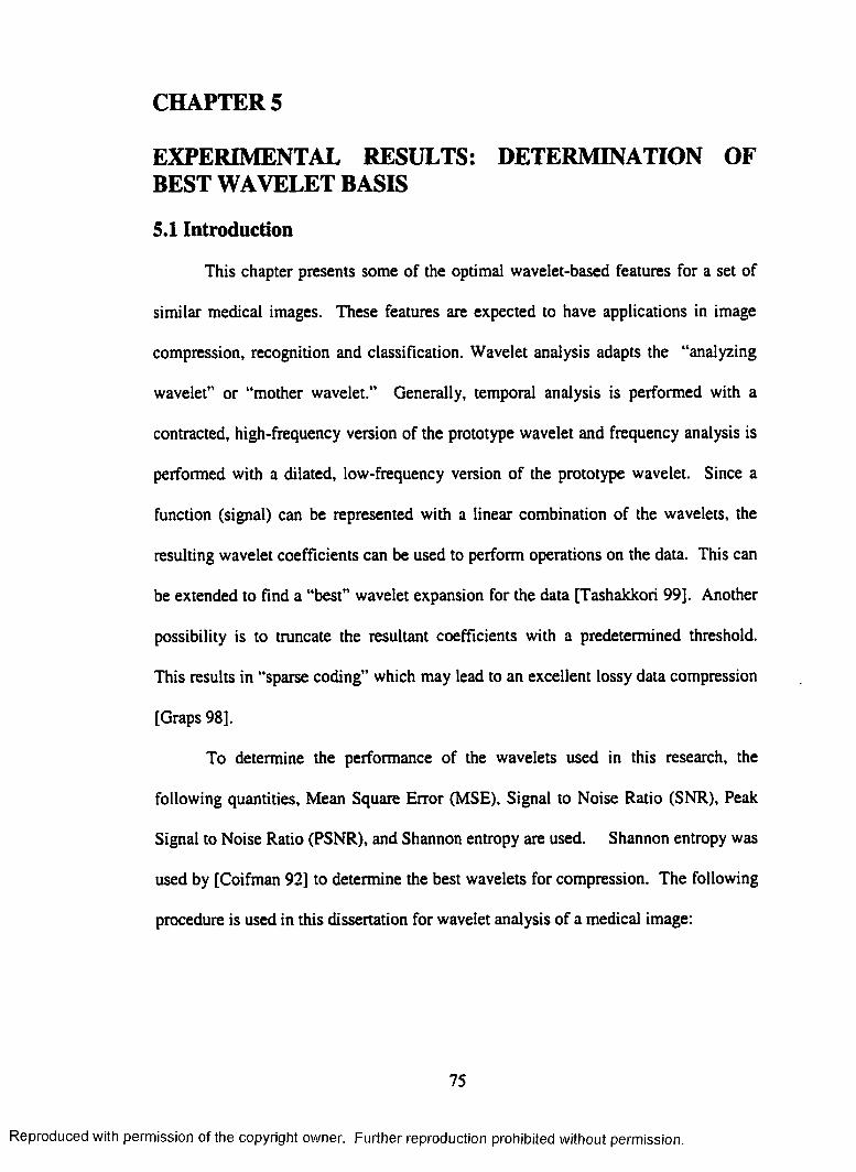
CHAPTERS
EXPERIMENTAL RESULTS: DETERMINATION OF BEST WAVELET BASIS
5.1 Introduction
This chapter presents some of the optimal wavelet-based features for a set of
similar medical images. These features are expected to have applications in image
compression, recognition and classification. Wavelet analysis adapts the “analyzing
wavelet” or “mother wavelet.” Generally, temporal analysis is performed with a
contracted, high-frequency version of the prototype wavelet and frequency analysis is
performed with a dilated, low-frequency version of the prototype wavelet. Since a
function (signal) can be represented with a linear combination of the wavelets, the
resulting wavelet coefficients can be used to perform operations on the data. This can
be extended to find a “best” wavelet expansion for the data [Tashakkori 99]. Another
possibility is to truncate the resultant coefficients with a predetermined threshold.
This results in “sparse coding” which may lead to an excellent lossy data compression
[Graps 98].
To determine the performance of the wavelets used in this research, the
following quantities. Mean Square Error (MSE), Signal to Noise Ratio (SNR), Peak
Signal to Noise Ratio (PSNR), and Shannon entropy are used. Shannon entropy was
used by [Coifman 92] to determine the best wavelets for compression. The following
procedure is used in this dissertation for wavelet analysis of a medical image:
75
Reproduced with permission of the copyright owner. Further reproduction prohibited without permission.
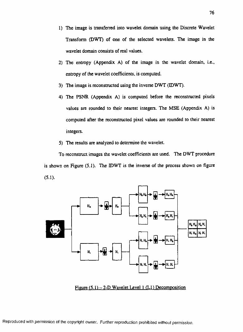
76
1) The image is transferred into wavelet domain using the Discrete Wavelet
Transform (DWT) of one of the selected wavelets. The image in the
wavelet domain consists of real values.
2) The entropy (Appendix A) of the image in the wavelet domain, i.e.,
entropy of the wavelet coefficients, is computed.
3) The image is reconstructed using the inverse DWT (EDWT).
4) The PSNR (Appendix A) is computed before the reconstructed pixels
values are rounded to their nearest integers. The MSE (Appendix A) is
computed after the reconstructed pixel values are rounded to their nearest
integers.
5) The results are analyzed to determine the wavelet.
To reconstruct images the wavelet coefficients are used. The DWT procedure
is shown on Figure (5.1). The IDWT is the inverse of the process shown on figure
(5.1).
He
HeH,
tfcH.
t
h i
H e H » n
HeH -
H,
H.H,
H.H.
H>Ho H.H,
H, He H.H.
Figure (5.1) - 2-D Wavelet Level 1 (LP Decomposition
Reproduced with permission of the copyright owner. Further reproduction prohibited without permission.

77
In this chapter, several sets of MRI and CT medical images are analyzed. The
results for MRI brain image sets in sagittal plane (es image set), in transverse plane (et
image set), and in coronal plane (eb image set) are presented. The results for two CT
image sets, one of the brain and the other of the spleen are also presented.
5.2 The es MRI-Set
The Mean Square Error (MSE), Peak Signal to Noise Ratio (PSNR), and
entropy analysis for the MRI-Set in sagittal plane follow.
5.2.1 Mean Square Error (MSE)
This set consists of 22 MRI images in sagittal plane. The results of MSE
analysis of the images at 5 different levels of decomposition are shown on Figures
(5.2) through (5.6). These Figures compare the MSE between the image reconstructed
with different wavelets and the original image. Figure (5.2) represents the MSE when
the image is reconstructed after one level of decomposition. Similarly, Figure (5.3)
through (5.6) represent, respectively, the MSE when the images are reconstructed after
2.3 ,4 , and 5 levels of decomposition.
For all Figures presented in this chapter, dbN denotes the Daubechies wavelet
with N coefficients, coN denotes the Coiflet with N coefFicients, biNM denotes the
biorthogonal wavelet with N vanishing moments for the high-pass synthesis Filter and
M vanishing moments for the high-pass analysis Filter, and syN denotes the Symlet
with N coefficients.
Reproduced with permission of the copyright owner. Further reproduction prohibited without permission.

78
0.004 0.0035
0.003 0.0025
$ 0.002 0.0015
0.001 0.0005
0 I0 1 2 3 4 5 6 7 8 9 10 11 12 13 14 15 16 17 18 19 20 21 22
Image Number
Figure (5.21 - Mean square error between the original and reconstructed images of the es set after i level of decomposition.
*
0.015
0.01
0.005
0 1 2 3 4 5 6 7 8 9 10 11 12 13 14 15 16 17 18 19 20 21 22
Image Number
Figure (5.3) - Mean square error between the original and reconstructed images of the es set after 2 levels of decomposition.
—e —db04 — db08 db12 db16 db20 - e — coOl —<— co02
■ co03 —— co04 —e— coQ5 sy04 sy08 sy12 sy16
bit 3 bi15 b i2 2 ---b i 2 4 bi26 bi28 — bi31
bi35 —* — bi39 bi44 —I— bi55 bi68
—e— db04 db08 db12 - db16 —m— db20 - e — co01 —t— co02—■— co03 - co04 co05 sy04 sy08 sy12 sy16
bi13 bi15 —-— b i2 2 bi24 bi26 bi28 bi31bi35 -Ha— bi39 bi44 —i— bi55 bi68
Reproduced with permission of the copyright owner. Further reproduction prohibited without permission.
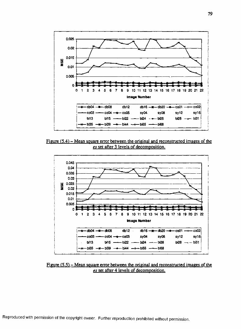
79
0.025
0.02
0.015
0.01
0.005
0 *
Image Number
db08co04
bi15
bi39
co02
sy16
bi31
db04
co03db12co05
bi22
bi44
db16
sy04
bi24
bi55
db20
sy08
bi26
bi68
co01
sy12
bi28
bi35
Figure (5.4) - Mean square error between the original and reconstructed images of the es set after 3 levels of decomposition.
0.0450.04
0.0350.03
iu 0.025 (0S 0.02
0.015 0.01
0.005
Image Number
db04
co03
bi13
bi35
db08co04
bi15
bi39
db12
co05
db20
sy08
co01
sy12
bi28 —^— bi31
co02
sy16
db16 sy04
bi22 bi24 — bi26
bi55 — bi68bi44
Figure (5.5) - Mean square error between the original and reconstructed images of the es set after 4 levels of decomposition.
Reproduced with permission of the copyright owner. Further reproduction prohibited without permission.
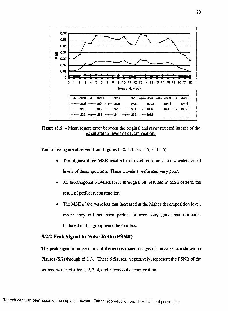
80
0.07
0.06
0.05
$ 0 04 * 0.03
0.02
0.01
! ■ i — 1 ■ * i 1 -1 4 i — a i i
Im age Number
co02{
sy16
db04
co03 — — co04 bi13
bi35
db06 db12 db20
syOS
co01
sy12 bi28 bi31
db16
co05 sy04bi15 bi22 bi24 bi26
b(39 bi44 bt55 bi68
Figure (5.6) - Mean square error between the original and reconstructed images of thees set after 5 levels of decomposition.
The following are observed from Figures (5.2, 5.3, 5.4,5.5, and 5.6):
• The highest three MSE resulted from co4, co3, and co5 wavelets at all
levels of decomposition. These wavelets performed very poor.
• All biorthogonal wavelets (bi 13 through bi68) resulted in MSE of zero, the
result of perfect reconstruction.
• The MSE of the wavelets that increased at the higher decomposition level,
means they did not have perfect or even very good reconstruction.
Included in this group were the Coiflets.
5.2.2 Peak Signal to Noise Ratio (PSNR)
The peak signal to noise ratios of the reconstructed images of the es set are shown on
Figures (5.7) through (5.11). These 5 figures, respectively, represent the PSNR of the
set reconstructed after 1, 2 ,3 ,4 , and 5 levels of decomposition.
Reproduced with permission of the copyright owner. Further reproduction prohibited without permission.
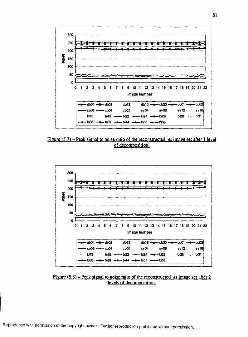
0 1 2 3 4 5 6 7 8 9 10 11 12 13 14 15 16 17 18 19 20 21 22
(mage Number
— db04 —■— db08 db12 db16 —* — db20
— ■— co03 -------co04 co05 sy04 sy08bi13 bi15 -------bi22 -------bi24 — bi26
—*— bi35 — bi39 —• — bi44 —I— bi55 — bi68
-co01 •
sy12
bi28
-co02
sy16
bi31
Figure C5.7) - Peak signal to noise ratio of the reconstructed es image set after 1 level of decomposition.
4- » . f - 1 — 1 1 1 1 4 " •(■ t - I— H t - i —1
• • _ • - - • - . — — - ■ - - _ (r- — - • _• _ • • • •_=
I , , 10 1 2 3 4 5 6 7 8 9 10 11 12 13 14 15 16 17 18 19 20 21 22
Im age Number
I—• — db04 —e — db08 db12 db16 db20 co01 —1— co02i
— — c o 0 3 — ■— co04 co05 sy04 sy08 sy12 sy16
j - bi13 bi15 ------- bi22 ------- bi24 — bi26 bi28 bi31 |
j—94— bi35 bi39 — bi44 —i— bi55 b6fi |
Figure (5.8) - Peak signal to noise ratio of the reconstructed es image set after 2 levels of decomposition.
Reproduced with permission of the copyright owner. Further reproduction prohibited without permission.
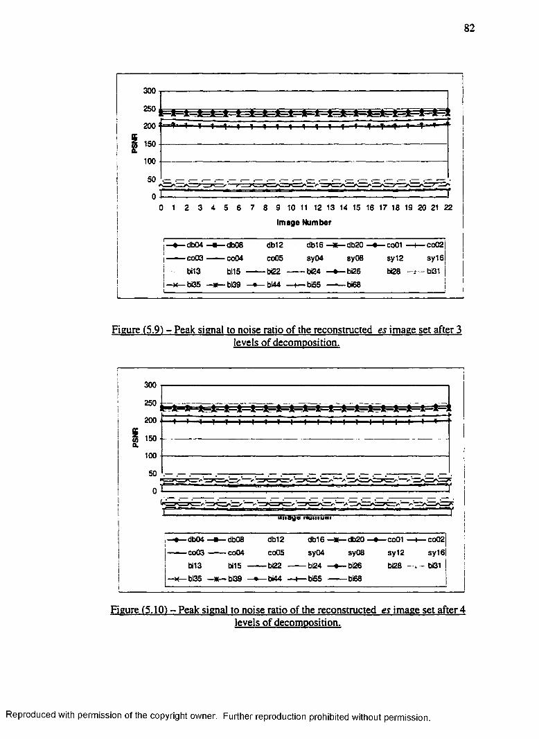
0 1 2 3 4 5 6 7 8 9 10 11 12 13 14 15 16 17 18 19 20 21 22
Im age Number
♦— db04 —* — db08 db12 db16 db20 - * - c o 0 1 —*— co02
j— — co 0 3 — ■— co04 co05 sy04 sy08 sy12 sy16
j bi13 bi15 bi22 bi24 — bi26 bi28 — — bi31
I—**— bi35 bi39 —•— bi44 —i— bi55 — — bi68 j1____________________________________________________ J
Figure (5.9) - Peak signal to noise ratio of the reconstructed es image set after 3levels of decomposition.
i
j 300 i--------------------------------------------------------------------------------------------------------------
200 . < f 1 - 1 — 1 —1— T1 —1— 1— 1 - I--. I — H--I— 1-—I - I - I - ■!■ ■■ I 1 — •
| 150--------------------------------------------------------------------------------------------------------------a.
1 0 0---------------------------------------------------------------------------------------------------------------
50
00 1 2 3 4 5 6 7 8 9 10 11 12 13 14 15 16 17 18 19 20 21 22
Image Number
—♦ — db04 db08 db12 db16—* — db20 —e— co01 — I— co02
— ■— co03 -------co04 co05 sy04 sy08 sy12 sy16bi13 bi15 ------- bi22 -------bi24 —• — bi26 bi28 - bi31
— — bi35 —* — bi39 — bi44 —I— b<55 ------- bi68
Figure (5.10) - Peak signal to noise ratio of the reconstructed es image set after 4levels of decomposition.
i t ~ t — t — I — f c A 1 - 1 —1 - t H - 1 — t■ t i —i—1—i—1- 1—i —i —i—)— 1 ■ i i
Reproduced with permission of the copyright owner. Further reproduction prohibited without permission.
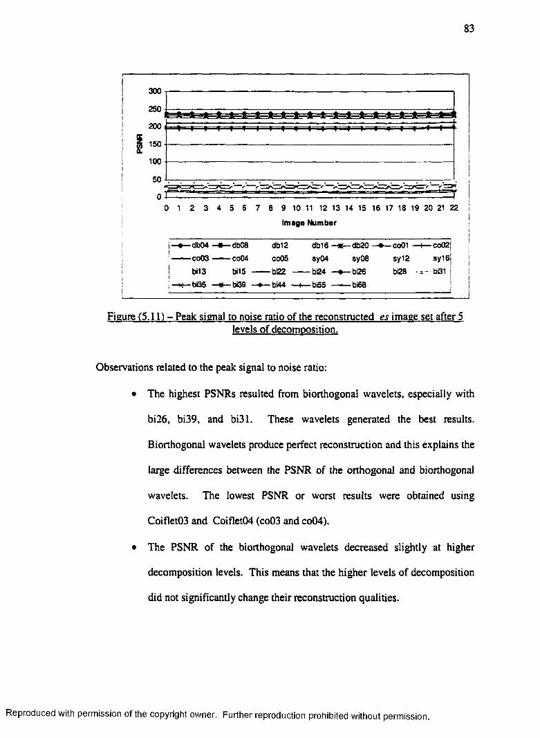
83
300
250
200 iI A 'ft IrrJL JL_ft* 1— ^
-<i-=*=T 4- T ~r 1-4 1- -T f- ? V 1 ~4 I f r 1" 1' <■150
100
0 1 2 3 4 5 6 7 8 9 10 11 12 13 14 15 16 17 18 19 20 21 22
Image Number
-db04-co03
bi13-bi35
•db08
-co04
bi15
-bi39
db12
co05
■bi22-bi44
db16 ■
sy04
- bi24 ■
-b£5
-db20
sy08
-bi26-bi68
-co01 —l— co02|
sy12 sy16
bi28 -* --b i3 1
Figure (5.11) - Peak signal to noise ratio of the reconstructed es image set after 5levels of decomposition.
Observations related to the peak signal to noise ratio:
• The highest PSNRs resulted from biorthogonal wavelets, especially with
bi26, bi39, and bi31. These wavelets generated the best results.
Biorthogonal wavelets produce perfect reconstruction and this explains the
large differences between the PSNR of the orthogonal and biorthogonal
wavelets. The lowest PSNR or worst results were obtained using
Coiflet03 and Coiflet04 (co03 and co04).
• The PSNR of the biorthogonal wavelets decreased slightly at higher
decomposition levels. This means that the higher levels of decomposition
did not significantly change their reconstruction qualities.
Reproduced with permission of the copyright owner. Further reproduction prohibited without permission.

84
5.2 J Entropy
The entropy of the es image set is presented in this section. Figures (5.12) through
(5.16), respectively, present the entropy of wavelet coefficients at levels 1 through 5.
0 1 2 3 4 5 6 7 8 9 10 11 12 13 14 15 16 17 18 19 20 21 22 j
Image Number !
— db04 —e— db08 db12 db16 db20 —e— co01 —t— co02—— co03 ------ co04 co05 sy04 sy08 syl2 sy16—e— bi13 —*— bi15 — bi22 — bi24 - - bi26 bi28 - A —bi31
bi35 — bi39 —• — bi44 —(— bi55 -------b(68
Figure (5.12) - Entropy of es set in the wavelet domain after the 1st level ofdecomposition.
0 1 2 3 4 5 6 7 8 9 10 11 12 13 14 15 16 17 18 19 20 21 22
Image Number
—e—db04 — db08 db12 db16 db20 — C001 —1— co02— — CO03 ------ co04 co05 sy04 sy08 sy12 syi6—e— bit3 —*—bi15 -------bi22 ------ bi24 - * - bi26 bi28 —e —bQi— bi35 —K—bi3S —•— b»44 —♦— bi55 -------bi68
Figure (5.13) - Entropy of es set in the wavelet domain after the 2nd level ofdecomposition.
Reproduced with permission of the copyright owner. Further reproduction prohibited without permission

85
5.4
4.8
4.4
4.2
Image Number
—• — d b 0 4 - * — db08 db12 db16 — db20 co01 —t— co02
— ■— co 0 3 co04 co05 sy04 sy08 sy12 sy16
—e— bi13 —*— bi15 bi22 bi24 —•— bi26 bi26 — bi31
—x— bi35 —x— bi39 bi44 —f —bi55 bi68
Figure (5.14) - Entropy of es set in the wavelet domain after the 3rd level of decomposition.
5.4
5.2
4.8
4.4
4.2
Image Number
db12
co05
bi22bi44
db16sy04
bi24
bi55
db04c o 0 3 co04
bi13 —*— bilS bi35
db08 db20
sy08bi26
bi68
co02
sy16bQ1
co01sy12
bi28
Figure (5.15) - Entropy of es set in the wavelet domain after the 4th level of decomposition.
Reproduced with permission of the copyright owner. Further reproduction prohibited without permission.

86
5.4
5.2
a 4.801 4.6
4.4
4.2
Image Number
db04 db08
co03 — — co04
bi13
bi35
db16 — db20
sy08
- bi26
bi55 --------b(68
db12
co05 sy04bi15 — — bi22 --------b(24
bi39
co01
sy12
bi28
bi44
Figure C5.16) - Entropy of es set in the wavelet domain after the 5th level ofdecomposition.
The following observations are related to the entropies of the image sets.
• The lowest entropies (best results) were obtained with biorthogonal
wavelets bi44, bi55, and bi68 at the 5th level of decomposition. The
highest entropies were obtained with bi 13 and bi 15 at the 1st level of
decomposition.
• Entropy decreased as the level of decomposition increased up to the 5th
level. The lowest entropy for all wavelets used in this research was
obtained at the 5th level of decomposition.
• A close relationship exists between the entropy and the size of the
diagnostic region in the image. The first and last images of this set have a
smaller diagnostic region than other members of the set (see Appendix C).
Reproduced with permission of the copyright owner. Further reproduction prohibited without permission.

The same relationship between entropies and the size of background
surrounding the diagnostic area can be observed. Thus, it seems that
larger background area resulted in a lower entropy.
5.3 The eb MRI-Set
The Mean Square Error (MSE), Peak Signal to Noise Ratio (PSNR), and
entropy analysis for the eb MRI-Set (23 MRI images) in the coronal plane follow.
5.3.1 Mean Square Error
The MSE analysis of the images at 5 different levels of decomposition are
presented on Figures (5.17) through (5.21). These Figures compare the MSE between
the image reconstructed by different wavelets and the original image. These Figures,
respectively, represent the MSE when the images are reconstructed after 1, 2, 3 , 4,
and 5 levels of decomposition.
0.005 0.0045
0.004 0.0035
0.003ill« 0.0025
0.002 0.0015 0.001
0.0005 0
0 1 2 3 4 5 6 7 8 9 10 11 12 13 14 15 16 17 18 19 20 21 22 23
Image Number
db04 db08 db12 db16 db20 —e— co01 —(— co02j
— co03 — co04 co05 sy04 sy08 sy12 sy16bi13 bi15 — — b i2 2 bi24 — bi26 bi28 - bi31
— bi35 bi39 bi44 —I— bi55 bi68
Figure (5.17) - Mean square error between the original and reconstructed images of the eb set after 1 level of decomposition.
permission of the copyright owner. Further reproduction prohibited without permission.

88
0.016
0.014
0.012
0.01
0.008
0.006
0.004
0.002
Image Number
co02sy16
i— db20
sy08
- bi26
— b»6S
db04
co03
bi13
bi35
db08co04
db12
co05
db16
sy04
bi22 bi24
bi55
co01
sy12
bi28bi15
b«39 —* — bi44
Figure (5.18) - Mean square error between the original and reconstructed images of ________________ the eb set after 2 levels of decomposition._______________
0.03
i0.025
0.02!
« 0.015
0.01
0.005
I0 1 2 3 4 5 6 7 8 9 10 11 12 13 14 15 16 17 18 19 20 21 22 23
Image Number
— db04 - e — db08 db12 db16 db20 co01 — co02
——- co03 —— co04 co05 sy04 sy08 sy12 sy16
bi13 bi15 bi22 bi24 — bi26 bi28 - » • - bi31—* -b i3 5 - * — bi39 — bi44 —t— bS5 --------bt68
Figure (5.19) - Mean square error between the original and reconstructed images of the eb set after 3 levels of decomposition.
Reproduced with permission of the copyright owner. Further reproduction prohibited without permission.
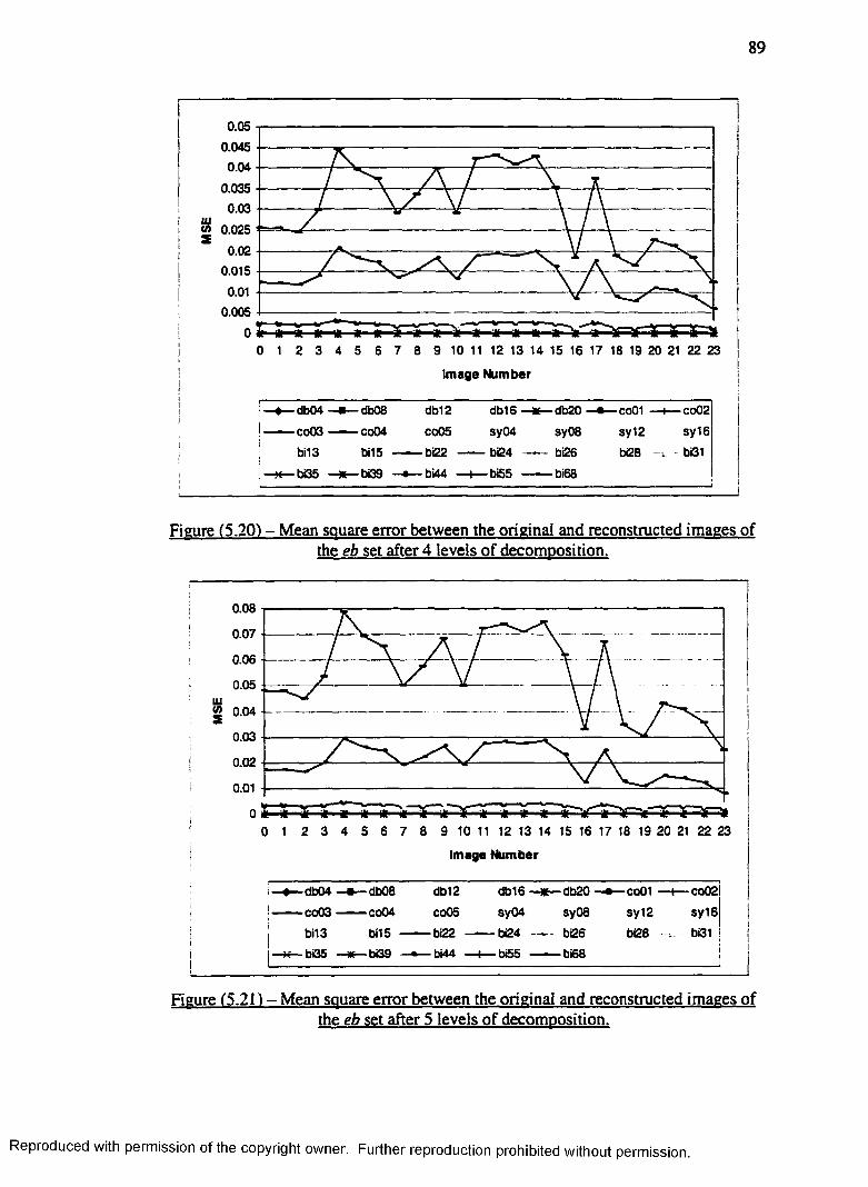
89
0.05 t—0.045 ----
0.04 - —
0.035----0 .0 3 ----
0.025 ’ ^
0.02 ----0.015----
0.01 ■ —
0.005 —
Im age Number
j — db04 —e— db08 db12 db16 db20 — co01 —*— co02
j— ■— co03 —— co04 co05 sy04 sy08 sy12 sy16
j bi13 bi15 bi22 bi24 bi26 bi28 . - bi31
j—x— bi35 bi39 bi44 —I— bi55 bl68
Figure (5.20) - Mean square error between the original and reconstructed images of the eb set after 4 levels of decomposition.
0.08
0.07
0.06
0.05
S2 0.04 ■ —
0.03
0.02
0.01
o lit * - i ~«~V
Image Num ber
db08co04
bi15bi39
db12
co05
bi22bi44
db16sy04
bi24bi55
db20
sy08bt26
bi68
co02
sy16bi31
db04co03
bi13bi35
co01
sy12bi28
Figure (5.21) - Mean square error between the original and reconstructed images of the eb set after 5 levels of decomposition.
Reproduced with permission of the copyright owner. Further reproduction prohibited without permission.

90
Observations related to Figures (5.17,5.18,5.19,5.20, and 5.21):
• The largest three MSEs were produced by Coiflets co4, co3, and co5 at all
levels of decomposition; they performed poorly.
• Biorthogonal wavelets, bil3, bil5, bi22,. . . , bi68 produced a MSE of zero
which is attributed to producing perfect reconstruction.
• The MSE increased at the higher decomposition levels for wavelets that
produced high MSE at lower levels of decomposition. The higher levels
of decomposition do not improve the quality of reconstruction.
5.3.2 Peak Signal to Noise Ratio
The peak signal to noise ratios of the reconstructed images of the es set are
shown on Figures (5.22) through (5.26). These images present, respectively, the
PSNR of the reconstructed set after 1 ,2 ,3 ,4 , and 5 levels of decomposition.
J 300
250
200
150
100
50
0
Figure (5.22) - Peak signal to noise ratio of the reconstructed eb image set after 1level of decomposition.
0 1 2 3 4 5 6 7 8 9 10 11 12 13 14 15 16 17 18 19 20 21 22 23
Image Number
db04 —• — db08 dbi2 db16 db20co03 — —C0G4 CO05 sy04 sy08bi13 bins ------ bi22 -----bi24 —e— bi26bi35 — bi39 —• — W44 —t— b»55 —— bi68
-co01 —i— co02! Isy12 syl6j 1
bi28 bi3l i
Reproduced with permission of the copyright owner. Further reproduction prohibited without permission.

91
300
250
200
150
100
»—»--t * t | t ~T~ 1 ■ — t —«=»■
0 1 2 3 4 5 6 7 8 9 10 11 12 13 14 15 16 17 18 19 20 21 22 23
Im age Number
-db04 —a— db08 db12 db16 db20 - e — co01 —<— co 0 2 -------- co03
co05 sy04 sy08 sy12 sy16 - - bi13 bi15 - bi22
-bi26 bi28 ~r. - bi31 — — bi35 bi39 bi44 —I— bi55 --------- b«68
Figure (5.23) - Peak signal to noise ratio of the reconstructed eb image set after 2 levels of decomposition.
300
250
200
150
100
50
>-#—» i i v 4 - 1 1 4 - 1 1 t n 1 -4- +■ <? 1 1 1 ' •
J0 1 2 3 4 5 6 7 8 9 10 11 12 13 14 15 16 17 18 19 20 21 22 23
Im age Num ber
-db04-co03
bi13-bi35
-db08-co04bi15
-bi39
db12co05
-bi22-bi44
db16sy04
-bi24-bi55
-db20sy08
-bi26-bi68
• co01 — i— co02 sy12 sy16 bi28 - i - bi31 j
Figure (5.24) - Peak signal to noise ratio of the reconstructed eb image set after 3levels of decomposition.
Reproduced with permission of the copyright owner. Further reproduction prohibited without permission.

92
300
250
200
I i -»' 100
! 50
! 0 1 2 3 4 5 6 7 8 9 10 11 12 13 14 15 16 17 18 19 20 21 22 23
j Im age Numberi
j i — db04 db08 db12 db16 db20 - e — cooTI ■ — -— co03 co04 co05 sy04 sy08 sy12
j bi13 bi15 bi22 — -b i2 4 bi26 bi28i bi35 bi39 bi44 —I— bi55 -------- b£8
Figure (5.25) - Peak signal to noise ratio of the reconstructed eb image set after 4 levels of decomposition.
j "" ~ ' ‘ ■ |
300 -------------------------------------------------------------------------------------------------------------
250 ---------------------------------------------------------------------------------------------------------------------------------s.--------------- It — i — t — i — - A j
j 200 a 1- 1— > - I - H— )— 1— 1—- I - 1 - 4 - 1 '1— 4— 1— 1— I— 1 • |
! \ 1 5 0 ---------------------------------------------------------------------------------------------------------------------ia. !
I1 0 0 -------------------------------------------------------------------------------------------------------------------- I
I
5 0 ...................................................r . • : ■ • ■
! Q
I 0 1 2 3 4 5 6 7 8 9 10 11 12 13 14 15 16 17 18 19 20 21 22 23
j Im age Number
i —e— db04 —e— db08 db12 db16 db20 - e — coOl"I| - c o 0 3 co04 co05 sy04 sy08 sy12| bi13 bi15 bi22 bi24 bi26 bi28| bi35 bi39 bi44 —I— bi55 bi68
Figure (5.26) - Peak signal to noise ratio of the reconstructed eb image set after 5 levels of decomposition.
—i— co02 sy 1 6 ;
— b(31 |
|—i . 1—I -I- H—)—1—1—-I- 1 -4 -1 '1—4—1—1—I—
X I ' ----------
—I— co02j syi61 bi31 |
Reproduced with permission of the copyright owner. Further reproduction prohibited without permission.

Observations related to Figures (5.22, 5.23,5.24, 5.25, and 5.26):
• The PSNR produced by biorthogonal wavelets was the largest (best
results). In particular, bi26, bi39, and bi31 had larger PSNR than the other
biorthogonal wavelets. Again, this can be attributed to biorthogonal
wavelets having perfect reconstruction. A large difference exists between
the PSNR of the orthogonal and biorthogonal wavelets. The lowest PSNR
(the worst results) were obtained with Coiflets (03 and 04).
• The PSNR of the biorthogonal wavelets slightly decreased at the higher
levels of decomposition. The higher levels of decomposition do not
significantly change the quality of reconstruction.
5.3.3 Entropy
The entropy of the images of the eb set in the wavelet domain is presented on
Figures (5.27 through 5.31). These figures, respectively, present the entropy of
wavelet coefficients at level 1 ,2 ,3 ,4 , and 5.
5.5
CL
3.5
(m a g * K i m b i r
—• — db(M - COQ3
1*13 —w— bi35
- • — <*>08--------CO04—• — <*15
1*39
db12co05
-------- 0(220 * 4
<*>16 sy04
— b<24 — 1— 0(55
—* — <*>20 sy06
- 0(26 — 0(68
• coO t sy 1 2 OfiB
— <— coQ2 sy16
—*— 0(31
Fieure (5.27) - Entropy of eb set in the wavelet domain after 1 level ofdecomposition.
permission of the copyright owner. Further reproduction prohibited without permission.

94
aowfi
0 1 2 3 4 5 6 7 8 9 10 11 12 13 14 15 16 17 18 19 20 21 22 23
Im age Number
— db04 db08 db12 db16 — db20 —e— co01 —i— co02— ■— co03 -------co04 co05 sy04 sy08 sy12 sy16
bi13 —■— bil 5 -------bi22 — bi24 ------bi26 bi28 bi31bi35 —*— bi39 —•— bi44 —l— bi55 — ■— bi68
Figure (5.28) - Entropy of eb set in the wavelet domain after 2 level of
4.5
3.5
Image Number
-co 0 2sy16j
- bi31
db04co03bi13bi35
db08co04bi15bi39
db12co05bi22bi44
db16sy04bi24bi55
(— db20 sy08 bi26
— bi68
coOlsy12bi28
Figure (5.29) - Entropy of eb set in the wavelet domain after 3 levels of decomposition.
Reproduced with permission of the copyright owner. Further reproduction prohibited without permission.

95
0 1 2 3 4 5 6 7 8 9 10 11 12 13 14 15 16 17 18 19 20 21 22 23
Image Number
-db04 •co03 bi13 ■
-bi3S
-db08•co04•bi15•bi39
db12 db16co05 sy04
-bi22 bi24.bi44 —i— bi55
db20 —e— co01 sy08 sy12bi26 bi28b68
-co02 sy i$ b01 i
Figure (5.30) - Entropy of eb set in the wavelet domain after 4 levels of ________________________ decomposition.________________________
0 1 2 3 4 5 6 7 8 9 10 11 12 13 14 15 16
Image Number
17 18 19 20 21 22 23
db04 —■— db08 db12 db16 db20 —e— co01 — i— co02i1 — —-co03 -------co04 coOS sy04 sy08 sy12 sy ld
bi13 —« -b i1 5 — -— bi22 -------bi24 bi26 bi28 bi311j—K— bi35 bi39 bi44 —1— bi55 ------- bi68 j
Figure (5.31) - Entropy of eb set in the wavelet domain after 5 levels of decomposition.
Reproduced with permission of the copyright owner. Further reproduction prohibited without permission.
96
The observations related to Figures (5.27,5.28,5.29,5.30, and 5.31):
• The lowest entropies (the best results) were obtained with biorthogonal
wavelets bi44, bi55, and bi68 at the 5th level of decomposition. The
highest entropies (worst results) were also obtained with biorthogonal
wavelets bil3 and bil5 at the 1st level of decomposition.
• Entropy continued to decrease with higher levels of decomposition up to
the 5th level. In fact, for all the wavelets used, the lowest entropy for each
was obtained at their 5th level of decomposition.
• The entropy has a close relationship to the size of the diagnostic part in the
image. As one can observe (Appendix C) that the first and last images of
the set have a smaller diagnostic area than other images in the set while
the other images have larger diagnostic areas. The same behavior and
order exists for their entropies. The opposite relationship exists for the
entropies and their background size surrounding the diagnostic area.
Thus, the larger background size for an image the lower its entropy.
5.4 The et MRI-Set
The Mean Square Error (MSE), Peak Signal to Noise Ratio (PSNR), and
entropy analysis for the (22 MRI images) et MRI-Set in transverse plane follow:
5.4.1 Mean Square Error
The results of MSE analysis of the images at 5 different levels of
decomposition are shown on Figures (5.32 through 5.36). These figures, respectively,
represent the MSE after 1 ,2 ,3 ,4 , and 5 levels of decompositions.
Reproduced with permission of the copyright owner. Further reproduction prohibited without permission.

97
0.004
0.0035
0.003
0.0025 | 0.002 0.0015
0.001 0.0005
00 1 2 3 4 5 6 7 8 9 10 11 12 13 14 15 16 17 18 19 20 21 22
Im age Number
!—• — db0 4 —«— db08 db12 - db16 db20 co01 —t— co02
j — — co03 - co04 co05 sy04 sy08 sy12 sy16
| bi13 bi15 bi22 bi24 —♦— bi26 bi28 bi31
| —K— bi35 bi39 bi44 —f— bi55 ---------b68
Figure (5.32) - Mean square error between the original and reconstructed images of the et set after 1 level of decomposition.
0.015
0.01
0.005
Im age Number
Figure (5.33) - Mean square error between the original and reconstructed images of the et set after 2 levels of decomposition.
db04 - e — db08 db12 db16 — db20 e co01
co03 — ■— co04 —♦— co05 sy04 sy08 sy12
bi13 bi15 ------- bi22 ------ bi24 bi26 bi28
bi35 bi39 —• — bi44 —I— bS5 ------- bi68
-co02
sy16bi31
Reproduced with permission of the copyright owner. Further reproduction prohibited without permission.

98
0.025
0.02
0.015
0.01
0.005
Im age Number
db04
co03
bi13
bi35
db08 co04 bil 5
bi39
db12 - db16
co05
bi22 b)44
db20 co01
sy12bi28
co02|
sy16bi31
sy04
bi24 — bi26
bi68
sy08
Figure (5.34) - Mean square error between the original and reconstructed images of the et set after 3 levels of decomposition.
0.035
0.03 -
0.025
0.02
0 .0 1 5 ------>
0.01 ■ —
0.005
Im age Number
— db04 db08 d b l i db16 — db20 - e — co01 —t— co02
- co03 - co04 ♦ co05 sy04 sy08 sy12 sy16
bi13 bil 5 bi22 b i 2 4 bi26 bi28 bi31——bi35 bi39 bi44 —I—bi55 —— bi68
Figure (5.35t - Mean square error between the original and reconstructed images of the et set after 4 levels of decomposition.
Reproduced with permission of the copyright owner. Further reproduction prohibited without permission.

0.07
0.06
0.05
SK 0 04* 0.03
0.02
0.01
! i- I ■* t - - i 1 i — t - t - 1 - i — t - i - 1 — 1 t0
Image Number
— db04 —■— db08 db12 db16 — db20 —• — co01 —I— co02—— CO03 -------co04 —♦— co05 sy04 sy08 sy12 sy16
bi13 bi15 -------bi22 ------ bi24 bi26 bi28 bi31—K— bi35 — bi39 bi44 —1— bi55 -------bi68
Figure (5.36) - Mean square error between the original and reconstructed images of the et set after 5 levels of decomposition.
Observations related to Figures (5.32,5.33,5.34, 5.35, and 5.36):
• The largest three MSEs were produced by co4, co3, and co5 at all levels of
decomposition; they perform very poorly.
• Biorthogonal wavelets, bi 13 bi68 produced a MSE of zero which is
attributed to producing perfect reconstruction.
• The MSE increased at the higher decomposition levels for wavelets that
produced high MSE at lower levels of decomposition. The higher levels
of decomposition did not improve the quality of reconstruction.
5.4.2 Peak Signal to Noise Ratio
The peak signal to noise ratios of the reconstructed images of the et set are
presented on Figures (5.37 through 5.41). These images present, respectively, the
PSNR of the reconstructed set after 1 ,2 ,3 ,4 , and 5 levels of decomposition.
with permission of the copyright owner. Further reproduction prohibited without permission.

100
300
250
200
150
100
50
0
« < ..n ir i ir -n n i i i t t i i i i i *—*■
0 1 2 3 4 5 6 7 8 9 10 11 12 13 14 15 16 17 18 19 20 21 22
Image Number
|—♦— db04 —«— db08 db12 db16 —K— db20 —e— co01 — i— co02
| — — co03 — — co04 co05 sy04 sy08 sy12 sy16j bil 3 bi15 -------bi22 — — bi24 bi26 bi28 - t bi31— bi35 —Xf— bi39 —* — bi44 —+— bi55 — bi68
Figure (5.37) - Peak signal to noise ratio of the reconstructed et image set after 1 level of decomposition.
300
250
200
150
100
50
ot0 1 2 3 4 5 6 7 8 9 10 11 12 13 14 15 16 17 18 19 20 21 22
Image Number
i- db04 —e— db08 db12 db16 - * t— db20co03 ------- co04 co05 sy04 sy08
bi13 bi15 -------bi22 -------bi24 —e— bi26
bi35 bi39 bi44 —I— bi55 ------- bi68
-co01 •
sy12
bi28
-co02j
sy16
b01
Figure (5.38) - Peak signal to noise ratio of the reconstructed et image set after 2 levels of decomposition.
Reproduced with permission of the copyright owner. Further reproduction prohibited without permission.

, 0 1 2 3 4 5 6 7 8 9 10 11 12 13 14 15 16 17 18 19 20 21 22
Im age Number
db04 —e— db08 db12 db16 db20 —e— co01 — i— co02
c o 0 3 -------co04 co05 sy04 sy08 sy12 sy16
bi13 bi15 ------- bi22 -------bi24 — bi26 bi28 — bi31
bi35 — bi39 —• — bi44 —1— bS5 -------bi68
Figure (5.39) - Peak signal to noise ratio of the reconstructed et image set after 3 levels of decomposition.
300
250i & t - J l — 1 — t t — & — & — %—k—l— & — & — & — < !
.h—j —f i—i" i - 1—1- 4- ■!—t—f I * i t r - *- •s(0a.
0 1 2 3 4 5 6 7 8 9 10 11 12 13 14 15 16 17 18 19 20 21 22
Image Number
-db04 —e— db08
-c o 0 3 -------co04
bil 3 bi15 --bi35 —*— bi39
db12
co05
-bi22 -bi44 ■
db16
sy04
bB4
-bB5
-db20 ■
sy08
-bi26 -bi68
-co01 ■
sy12
bi28
-co02
sy16
bi31
Figure (5.401 - Peak signal to noise ratio of the reconstructed et image set after 4 levels of decomposition.
Reproduced with permission of the copyright owner. Further reproduction prohibited without permission.

102
300
250
200
150
100
Im age Number
db04
co03
bi13
db08CO04
db12CO05 sy04
bi15 bi22 —— bi24bi39
db16 db20
sy08
bi26
bS5 bi68
co01sy12bi28
co02|
sy16|
bi31 |
Figure (5.41) - Peak signal to noise ratio of the reconstructed et image set after 5levels of decomposition.
Observations related to Figures (5.36,5.37,5.38, 5.39, and 5.41):
• The PSNR produced by biorthogonal wavelets was the largest (best
results). In particular, bi26, bi39, and bi31 had larger PSNR than the other
biorthogonal wavelets. Again, this can be attributed to biorthogonal
wavelets having perfect reconstruction. A large difference exists between
the PSNR of the orthogonal and biorthogonal wavelets. The worst results
were obtained with Coiflets (03 and 04).
• The PSNR of the biorthogonal wavelets decreased slightly at the higher
levels of decomposition. The higher levels of decomposition do not
significantly change the quality of reconstruction.
Reproduced with permission of the copyright owner. Further reproduction prohibited without permission.

103
5.43 Entropy
The entropy of the images of the et set in the wavelet domain is presented on
Figures (5.42, 5.43, 5.44, 5.45, and 5.46). These figures, respectively, present the
entropy of wavelet coefficients at levels 1, 2, 3,4, and 5.
5.9
£ 5.8
5.6
5.5
5.4
Image Number
♦ ■ db04 —e— db08 db12 db16 — db20 —e — co 0 1 — i— co02|
— ■— co 0 3 co04 co05 sy04 sy08 sy12 sy16|
—e— bi13 —*— bi15 — — bi22 —-— bi24 bi26 bi28 bi31 !
— — bi35 bi39 bi44 —I— bi55 --------bi68 1
Figure (5.421 - Entropy of et set in the wavelet domain after the 1st level ofdecomposition.
The observations related to Figures (5.42, 5.43,5.44,5.45, and 5.46):
• The lowest entropies (the best results) were obtained with biorthogonal
wavelets bi44, bi55, and bi68 at the 5th level of decomposition. The
highest entropies (worst results) were obtained with biorthogonal wavelets
bil3 and bil5 at the 1st level of decomposition.
Reproduced with permission of the copyright owner. Further reproduction prohibited without permission.
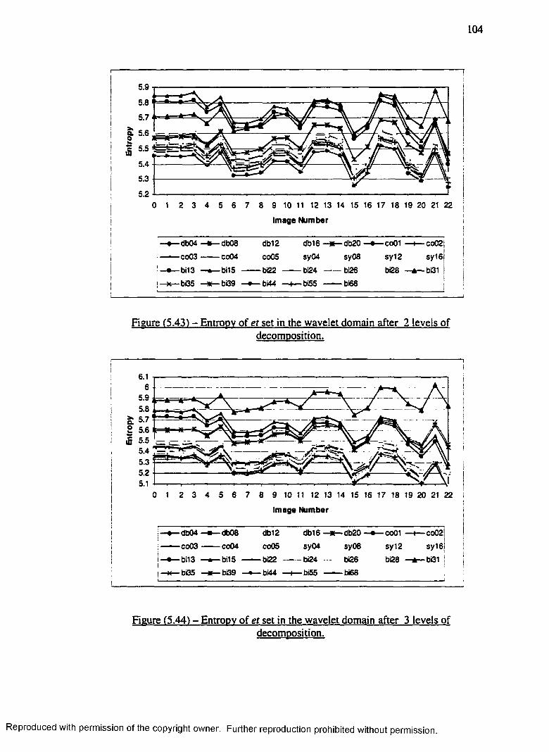
104
5.2 ---------------------------------- — I0 1 2 3 4 5 6 7 8 9 10 11 12 13 14 15 16 17 18 19 20 21 22 j
Image Number
— db04 —e— db08 db12 db16 db20 —e— co01 —i— co02—■— cc03 —— co04 co05 sy04 sy08 sy12 sy 16—• — bi13 —*— bi15 -------bi22 ------ bi24 ----- bi26 bi28 —*—bi31
bi35 bi39 —•— bi44 —(— bi55 ------ bi68
Figure (5.43) - Entropy of et set in the wavelet domain after 2 levels ofdecomposition.
0 1 2 3 4 5 6 7 8 9 10 11 12 13 14 15 16 17 18 19 20 21 22 I
Image Number
db04 —« — db08 db12 db16 — db20 —e— co01 — I— co02
co03 -------co04 co05 sy04 sy08 sy12 syi6
bi13 — bi15 ------- bi22 ------ bi24 — bi26 bi28 —A— bQ1bi35 bi39 —•— bi44 —1— bi55 -------bi68
i
Figure (5.44) - Entropy of et set in the wavelet domain after 3 levels ofdecomposition.
Reproduced with permission of the copyright owner. Further reproduction prohibited without permission.

105
0 1 2 3 4 5 6 7 8 9 10 11 12 13 14 15 16 17 18 19 20 21 22
Image Number
db04 - m — db08 db12 db16 —X— db20 — co01 — I— co02co03 ------- co04 co05 sy04 sy08 sy12 sy16bil 3 —6— bil 5 -------bi22 -------bi24 — — bi26 bi28 —A— bQ1 Ibi35 —M— bi39 —• — bi44 —I— bi55 -------bi68
Figure (5.45) - Entropy of et set in the wavelet domain after 4 levels of decomposition.
0 1 2 3 4 5 6 7 8 9 10 11 12 13 14 15 16 17 18 19 20 21 22
Image Num ber
— db04 db08 db12 db16 — db20 —e — co01 — co02
— ■— co 0 3 —-— co04 co05 sy04 sy08 sy12 sy16
—e— bi13 —*— bi15 -------- bi22 —— bi24 - - bi26 bi28 —A— bi31—K— b(35 — bi39 b(44 —I— bi55 bi68
Figure (5.461 - Entropy of et set in the wavelet domain after 5 levels of decomposition.
Reproduced with permission of the copyright owner. Further reproduction prohibited without permission.

• Entropy continued to decrease with higher levels of decomposition up to
the 5th level. For all wavelets used, the lowest entropy for each was
obtained at their 5th level of decomposition.
• The entropy has a close relationship to the size of the diagnostic part in the
image. As one can observe (Appendix C) the first images of the set have
larger diagnostic area while the last images have smaller diagnostic area.
The same behavior and order exists for their entropies. The opposite
relationship exists for the entropies and their background size surrounding
the diagnostic area. Thus, the larger the background size of an image the
lower its entropy.
5.5 The cc CT-Set
The Mean Square Error (MSE), Peak Signal to Noise Ratio (PSNR), and
entropy analysis for the (20 CT brain images) cc CT-Set follows.
5.5.1 Mean Square Error
The MSE analysis of the images at 5 different levels of decomposition are
presented on Figures (5.47 through 5.51). These figures, respectively, represent the
MSE between the original set and the reconstructed set after 1, 2, 3, 4, and 5 levels of
decomposition.
Observations related to Figures (5.47,5.48, 5.49,5.50, and 5.51):
• The largest three MSEs were produced by co4, co3, and co5 at all levels of
decomposition; they performed very poorly.
• Biorthogonal wavelets, bil3, ..., bi68 produced a MSE of zero which is
attributed to producing perfect reconstruction.
Reproduced with permission of the copyright owner. Further reproduction prohibited without permission.
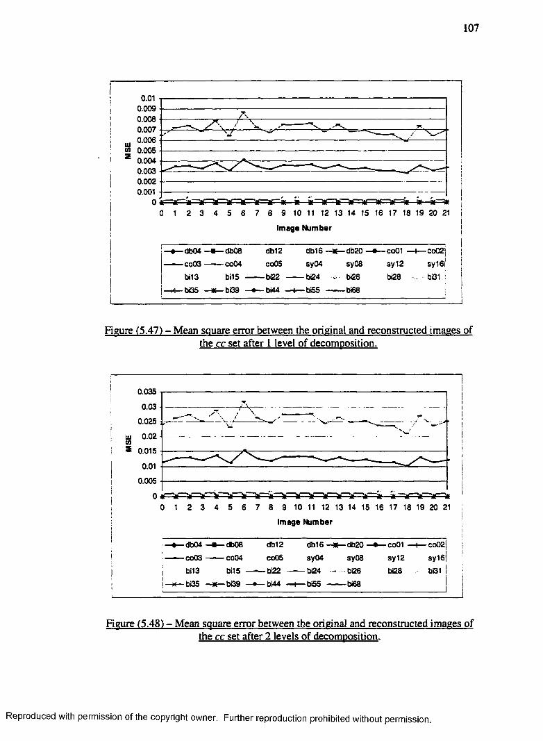
107
0.010.0090.0080.0070.0060.0050.0040.0030.0020.001
Image Number
— db04 —■— db08 db12 db16 db20 —• — co01 — — co02|— — co03 —— co04 co05 sy04 sy08 sy12 sy16|
bi13 bi15 ------- bi22 ------ bi24 bi26 bi28 . bi31 !
bi35 — bi39 —• — bi44 —+— bi55 ------- bi68 |
Figure (5.47) - Mean souare error between the original and reconstructed images of the cc set after 1 level of decomposition.
0.035
0.03
0.025
0.020.015
0.01
0.005
* at ■*
Image Number
db04 — db08 db12 db16 — db20 • coOl —i— co02]
co03 — — co04 co05 sy04 sy08 sy12 sy16|bi13 bil 5 — — bi22 — — bi24 ------bi26 bi28 , bi31
bi35 bi39 — bi44 — I— bi55 ------- bi68 I
Figure (5.48) - Mean square error between the original and reconstructed images of the cc set after 2 levels of decomposition.
Reproduced with permission of the copyright owner. Further reproduction prohibited without permission.

108
0.07
0.06
0.05
Uj 0.04
* 0.03
0.02
0.01
0 1 2 3 4 5 6 7 6 9 10 11 12 13 14 15 16 17 18 19 20 21
Image Num ber
j—♦— d b 0 4 - « — db08 d b i l - db16 db20 - e — co01 —f— co02[— co 0 3 co04 co05 sy04 sy08 sy12 sy16!
bil 3 bi15 bi22 bi24 —*-— bi26 bi28 bi31 |
— bi35 — bi39 — bi44 — i— bi55 bi68 j
Figure (5.49) - Mean sauare error between the original and reconstructed images of the cc set after 3 levels of decomposition.
0.12
0.1
0.08 — j v
0.06
0.04
0.02
0 *0 1 2 3 4 5 6 7 8 9 10 11 12 13 14 15 16 17 18 19 20 21
Image Num ber I— db04 - a — dt>08 db12 db16 db20 —e— co01 —i— co02|
- co03 ------- co04 co05 sy04 sy08 sy12 sy16jbi13 bits -------bi22 -------bi24 — bi26 bi28 - . - bi31 !Ibi35 —* — bi39 —• — b(44 —t— bi55 ------- bi68 I
Figure (5.50) - Mean square error between the original and reconstructed images of the cc set after 4 levels of decomposition.
Reproduced with permission of the copyright owner. Further reproduction prohibited without permission.

109
0.180.160.140.12
0.080.060.040.02
Image Number
dt>04 —m— db08
— ■— co 0 3 co04
bi13
—*— bi35
db12 db16
co05 sy04
b i1 5 bi22 bi24b(44
!— db20
sy08 - bi26
bt55 — bi68
coOl
sy12
co02
sy16
bi39
Figure (5.51) - Mean square error between the original and reconstructed images of the cc set after 5 levels of decomposition.
e The MSE increased at the higher decomposition levels for wavelets that
produced high MSE at lower levels of decomposition. The higher levels
of decomposition do not improve the quality of reconstruction.
5.5.2 Peak Signal to Noise Ratio
The peak signal to noise ratios of the reconstructed images of the et set are
presented on Figures (5.50 through 5.54). These images, respectively, present the
PSNR of the reconstructed set after 1 ,2 ,3 ,4 , and 5 levels of decomposition.
Reproduced with permission of the copyright owner. Further reproduction prohibited without permission.

110
fc-X— X— X— X— X— X— X—X—X—X— X—X— X— X— X—X—X—X— X—X—
I0 1 2 3 4 5 6 7 8 9 10 11 12 13 14 15 16 17 18 19 20 21
Image Number
— db04 —e— db08 db12 db16 — db20 — co01 —h— co02
— ■— c o 0 3 -------co04 co05 sy04 sy08 sy12 — sy16
| bi13 bil5 -------bi22 —— bi24 - - bi26 bi28 -bi31 j
bi35 —* — bi39 bi44 —I— bi55 — bi68 |
Figure (5.52) - Peak signal to noise ratio of the reconstructed cc image set after 1level of decomposition.
250x — a t — x — x — x — x — x — x — x — x — x — x — x — x — x — x — x
0 1 2 3 4 5 6 7 8 9 10 11 12 13 14 15 16 17 18 19 20 21
Image Number
- d b 0 4
•cc03bi13
-bi35
-db08
-co04
bi15 ■
-bt39
db12
co05
-bi22 -bi44 ■
db16 ■
sy04
■ bi24
-bi55 ■
-db20 •
sy08
bi26
•bi68
•coOl
sy12
bi28
—f -c o 0 2 |
—A—syisj - - bi31 I
Figure (5.53) - Peak signal to noise ratio of the reconstructed cc image set after 2levels of decomposition.
Reproduced with permission of the copyright owner. Further reproduction prohibited without permission.
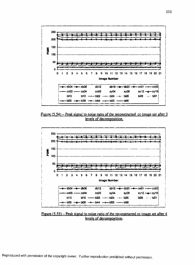
I l l
250
200
g 150 at
100
50
0
i x — x — x — x — x—x—i —k—i —t ■ * k—x—x—i.ii—'t — ^ i— * — * — 4— * — ^ — 4- - » — * — * — # — 4 — i n 4 -
0 1 2 3 4 5 6 7 8 9 10 11 12 13 14 15 16 17 18 19 20 21
Im age Number
db04 —e— db08 db12 db16 —Me—db20 —e — coOl — (— co02|
co03 -------co04 co05 sy04 sy08 sy12 —A— syiej
bi13 bil 5 -------bi22 -------bi24 bi26 bi28 - r - bi31
bi35 —X— bi39 — bi44 —t— bi55 -------bi68I
i
Figure (5.54) - Peak signal to noise ratio of the reconstructed cc image set after 3levels of decomposition.
2504C— X—X— X— X—!*—X— X=-X— X— X— X— Xr=X—X— X— X—X— X— X— X-rX
200 f - | r V T " T 1 I T 1 " - t 1" I '! 4 4 - f— 1 1— 4 1—+
150
° * 100
50
c =T0 1 2 3 4 5 6 7 8 9 10 11 12 13 14 15 16 17 18 19 20 21
Image Number
Figure (5.55) - Peak signal to noise ratio of the reconstructed cc image set after 4levels of decomposition.
Reproduced with permission of the copyright owner. Further reproduction prohibited without permission

Image Number
db04 db08 db12 db16 — db20 —• — co01
co03 -------co04 co05 sy04 sy08 sy12
bi13 bit 5 — ■— bE2 — bi24 bi26 bi28
bi35 bi39 —• — bi44 —4— b65 -------bi68
-co02|
-sy16! b(31 I
Figure (5.56) - Peak signal to noise ratio of the reconstructed cc image set after 5levels of decomposition.
Observations related to Figures (5.52,5.53,5.54,5.55, and 5.56):
• The PSNR produced by biorthogonal wavelets was the largest (best
results). In particular, bi26, bi39, and bi31 had larger PSNR than the other
biorthogonal wavelets. Again, this can be attributed to biorthogonal
wavelets having perfect reconstruction. A large difference exists between
the PSNR of the orthogonal and biorthogonal wavelets (the worst results)
were obtained with coiflets (03 and 04).
• The PSNR of the biorthogonal wavelets slightly decreased at the higher
levels of decomposition. The higher levels of decomposition do not
significantly change the quality of reconstruction.
permission of the copyright owner. Further reproduction prohibited without permission.

113
5.5.3 Entropy
The entropy of the images of the et set in the wavelet domain is presented on
Figures (5.57, 5.58, 5.59, 5.60, and 5.61). These figures, respectively, present the
entropy of wavelet coefficients at levels 1, 2 ,3 ,4 , and 5.
4-5
a4
3.5
Image Number
db04 db08
co03 — — co04
bil 3
bi35
db12
co05bi15 bi22
bi39
db16 co01
sy12bi28
co02|
sy is l bi31 !
sy04
b i 2 4 bi26
bi55 --------b68
sy08
Figure (5.571 - Entropy of cc set in the wavelet domain after 1 level ofdecomposition.
The observations related to Figures (5.57, 5.58,5.59, 5.60, and 5.61):
• The lowest entropies (the best results) were obtained with biorthogonal
wavelets bi44, bi55, and bi68 at the 5th level of decomposition. The highest
entropies (worst results) were also obtained with biorthogonal wavelets bil3
and bil 5 at the 1st level of decomposition.
Reproduced with permission of the copyright owner. Further reproduction prohibited without permission.

114
4.5
*• 3.5aotof i 3
2.5
0 1 2 3 4 5 6 7 8 9 10 11 12 14 15 16 17 18 19 20 21
Image Number
db04 db08 db12 - - db16 —K— db20 —• — co01 —l— co02
co03 — ■— co04 co05 sy04 sy08 sy12 sy16
bi13 —a —bi15 ------- bi22 -------bi24 —<— bi26 bi28 bi31bi35 —*— bi39 — bi44 —I— bS5 ------- b£8
Figure (5.58) - Entropy of cc set in the wavelet domain after 2 levels ofdecomposition.
4.5
3.5 - f t
2.5
Im age Number
co02
sy16
bi31
db04
co03
bi13bi35
dt>08
co04
bi15bi39
d b 1 2 db16
co05 bi22
bi44
db20
sy08
coOl
sy12
bi28sy04
b i 2 4 bi26
bS5 --------b£8
Figure (5.591 - Entropy of cc set in the wavelet domain after 3 levels ofdecomposition.
Reproduced with permission of the copyright owner. Further reproduction prohibited without permission.

115
4.5
3.5
Im age Number
!—• — db04 — db08 db12 db16 db20 — co01 —I— co02
|— — co 0 3 -------- co04 co05 sy04 sy08 sy12 sy16
i—- — bi13 — bi15 — bi22 bi24 —*-bc26 bi28 - bi31
i —K— bi35 — bi39 bi44 — I— bi55 bi68
Figure (5.60) - Entropy of cc set in the wavelet domain after 4 levels ofdecomposition.
4.5
nr3.5
2 *■
Im age Number
db04
co03bi13bi35
db12
co05bi22
bi44
db16
sy04bi24
bi55
db08
co04
bi15bi39
db20sy08
bi26
b£8
co01
sy12
bi28
— co02
sy16
— bi31
Figure (5.61) - Entropy of cc set in the wavelet domain after 5 levels ofdecomposition.
Reproduced with permission of the copyright owner. Further reproduction prohibited without permission.
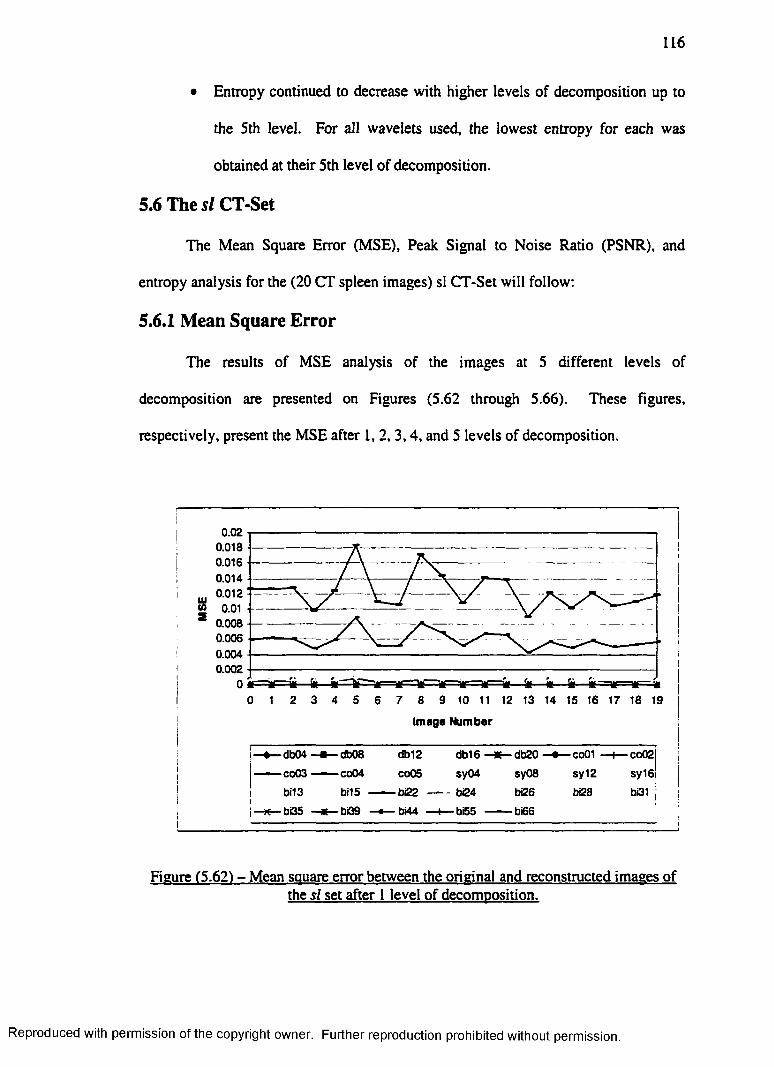
116
• Entropy continued to decrease with higher levels of decomposition up to
the 5th level. For all wavelets used, the lowest entropy for each was
obtained at their 5th level of decomposition.
5.6 The si CT-Set
The Mean Square Error (MSE), Peak Signal to Noise Ratio (PSNR), and
entropy analysis for the (20 CT spleen images) si CT-Set will follow:
5.6.1 Mean Square Error
The results of MSE analysis of the images at 5 different levels of
decomposition are presented on Figures (5.62 through 5.66). These figures,
respectively, present the MSE after 1, 2 ,3 ,4 , and 5 levels of decomposition.
0.020.0180.0160.0140.0120.01
0.0080.0060.0040.002
Image Number
co01
sy12
bi28
co02
sy16 bi31 !
— db04
—■— co03 —-— co04
bi13
— bi35
db12 db16
co05 sy04
bi15 b i2 2 bi24bi39
db20
sy08 bi26
bBS bi66bi44
Figure (5.62) - Mean square error between the original and reconstructed images of the si set after 1 level of decomposition.
Reproduced with permission of the copyright owner. Further reproduction prohibited without permission.

117
0.07
0.06
0.05
0.04
0.03
0.02
0.01
Image Number
db04
co03
bi13
bi35
db08
co04
bi15
bi39
db16
sy04
bi24
bS5
i—db20
sy08
— bi26
■— bi66
co02
sy16
bi31
db12
co05
bi22bi44
coOl
sy12
bi28
Figure (5.631 - Mean square error between the original and reconstructed images of the si set after 2 levels of decomposition.
0.14
0.12
0.1
0.08
0.06
0.04
0.02
Image Number
db16 db20sy08
bi26
bB6
co02
sy16
db04
co03
bi13bi35
db08co04
bi15
bi39
db12 co01
sy12co05 sy04
bi22 bi24
bi44 —h— b>55
Figure (5.641 - Mean souare error between the original and reconstructed images of the si set after 3 levels of decomposition.
Reproduced with permission of the copyright owner. Further reproduction prohibited without permission.

118
020.180.160.140.12
0.10.080.060.040.02
Image Number
db16
sy04
bi24
bi55
co02
sy16
db04
co03
bi13
bi35
db08
co04
bi15
bi39
db12
co05
bi22
bi44
db20
sy08
bi26bB6
co01
sy12
bi28 bi31
I__________________________________________________________________I
Figure (5.65) - Mean square error between the original and reconstructed images of the si set after 4 levels of decomposition.
0.35
0.3
0.25
SJ 02* 0.15
0.1
0.05
« — m !a~ ^y~ !a la k *
Image Number
i I—e— db04 db08 db12 db16 db20 co01 —t— co02j
—— co03 — co04 co05 sy04 sy08 sy12 sy16j
bi13 bi15 bi22 — b i2 4 bi26 bi28 . - bi31 j
! bi35 bi39 - ^ b i 4 4 —t— b65 --------bi66 !
Figure (5.661 - Mean square error between the original and reconstructed images of the si set after 5 levels of decomposition.
Reproduced with permission of the copyright owner. Further reproduction prohibited without permission.

119
Observations related to Figures (5.62,5.63,5.64,5.65, and 5.66):
• The largest three MSEs were produced by co4, co3, and co5 at all levels of
decomposition; they perform very poorly.
• Biorthogonal wavelets, bil3, ..., bi68 produced a MSE of zero which is
attributed to producing perfect reconstruction.
• The MSE increased at the higher decomposition levels for wavelets that
produced high MSE at lower level of decomposition. The higher levels of
decomposition do not improve the quality of reconstruction.
5.6.2 Peak Signal to Noise Ratio
The peak signal to noise ratios of the reconstructed images of the et set are
presented on Figures (5.67 through 5.71). These images, respectively, present the
PSNR of the reconstructed set after 1 ,2 ,3 ,4 , and 5 levels of decompositions.
ii300 -i
:— £— i — *— I — 1 — i — £— £— x— i — I — I — 1 — 1:— £— *— i — i —300 •
1*50
100
50
0 . . .................0 1 2 3 4 5 6 7 8 9 10 11 12 13 14 15 16 17 18 19
Im age Number
♦ - db04 e db06 db12 db16 —* — db20 —• — coOl —t— co02|
— ■— co03 —— co04 co05 sy04 sy08 sy12 sy16j
bil 3 bi15 bi22 — bi24 — bi26 b i2 8 bi31 i
—H— bi35 bi39 bi44 —i— bi55 —— bi66 \
Figure (5.61) - Peak signal to noise ratio of the reconstructed si image set after 1 levelof decomposition.
Reproduced with permission of the copyright owner. Further reproduction prohibited without permission.

120
300
250
200 1
150
100
1 i " t
X X X . X X X x - .
t=0 1 2 3 4 5 6 7 8 9 10 11 12 13 14 15 16 17 18 19
Image Number
-db04
*co03 ■
bi13
-bi35
-db08
-co04
bi15
-bi39
db12
co05
■b<22■bi44
db16sy04
bi24
-bB5
db20
sy08bi26
bi66
-co01
sy12
bi28
-co02
sy16bi31
Figure (5.681 - Peak signal to noise ratio of the reconstructed si image set after 2levels of decomposition.
300
250 ;
200 '
150
100
50
0 1 2 3 4 5 6 7 8 9 10 11 12 13 14 15 16 17 18 19
Im age Number
-db04
-co03 •
bi13
-bi35
-db08
•co04
bi15 •
•bi39
db12
co05-bi22-bi44
db16 ■
sy04 -bi24 •
•bB5 ■
•db20
sy08
-bi26
-bi66
•co01
sy12
bi28
-co02|
sy16|
bi31 jI
Figure (5.69) - Peak signal to noise ratio of the reconstructed si image set after 3levels of decomposition.
Reproduced with permission of the copyright owner. Further reproduction prohibited without permission.
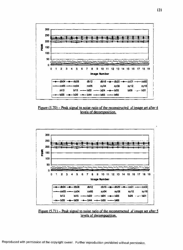
121
s(0a.
300
250;
200 i
150
100
50
0
- y r - T j . - » r j " 1 ' I» 1 ■ 1 - 4 - 1 1 1 1 I
= ■ * - ' , i ■ — ' = T
0 1 2 3 4 5 6 7 8 9 10 11 12 13 14 15 16 17 18 19
Image Number
-db04
-co03 •
bi13 ■bi35 •
-db08 • co04
bi15 ■
-bi39
db12
coOS -bi22 -bi44 •
db16 ■ sy04
-bi24 ■
-b65 ■
-db20 ■
sy08
■bi26
■bi66
-co01 •
sy12
bi28
-co02
sy16
bi31
Figure (5.70) - Peak signal to noise ratio of the reconstructed si image set after 4levels of decomposition.
300
250
200
150
100
50
0
1 ------ 4 — T ■ n ■» <r * ■•+ ~-4~
[—e— db04 —■— db08 db12 db16 —* — db20
1------- co03j — ■— co04 co05 sy04 sy08
j bi13 bi15 -------bi22 -------bi24 - e — bi26
! — — bi35 bi39 —•— bi44 —I— bi55 ------- bi66
0 1 2 3 4 5 6 7 8 9 10 11 12 13 14 15 16 17 18 19
Im age Number
-co01 — i— co02|
sy12 sy16|
bi28 —=— bi31
Figure (5.71) - Peak signal to noise ratio of the reconstructed si image set after 5levels of decomposition.
Reproduced with permission of the copyright owner. Further reproduction prohibited without permission.

Observations related to Figures (5.67,5.68,5.69,5.70, and 5.71):
• The PSNR produced by biorthogonal wavelets was the largest (best
results). In particular, bi26, bi39, and bi3I had larger PSNR than the other
biorthogonal wavelets. Again, this can be attributed to biorthogonal
wavelets having perfect reconstruction. A large difference exists between
the PSNR of the orthogonal and biorthogonal wavelets. The worst results
were obtained with Coiflets (03 and 04).
• The PSNR of the biorthogonal wavelets slightly decreased at the higher
levels of decomposition. The higher levels of decomposition do not
significantly change the quality of reconstruction.
5.63 Entropy
The entropy of the images of the et set in the wavelet domain is presented on
Figures (5.72, 5.73, 5.74, 5.75, and 5.76). These figures respectively present the
entropy of wavelet coefficients at levels 1 ,2 ,3 ,4 , and 5.
5.5-1-----5.3 -pA5.1 —4.9
>. 4 .7 + " -! i 4.5 £= = ifi 4.3 I— 1
4. 1 ------3. 9 ------3 .7 ------3 .5 ------
(mage Numbar
co02
sy16dbOSCO04
CO01 sy12
bS8 bi31
db04
co03bi13bQ5
db12co05 —•— sy04
bi15 — — b i2 2 bi24bt44 — i— bi55
Figure (5.721 - Entropy of si set in the wavelet domain after 1 level of decomposition.
permission of the copyright owner. Further reproduction prohibited without permission.

123
4.5
>•o
3.5
0 1 2 3 4 5 6 7 8 9 10 11 12 13 14 15 16 17 18 19
Im age Num ber
— db04 dt>08 db12 db16 —HE— db20 —e — co01 —I—-co02
—— co03 — ■— co04 co05 —•— sy04 sy08 sy12 sy16|
—• — bi13 — bi15 — bi22 -------bi24 —•— bi26 bi28 bi31 |
— bi35 —* — bQ9 ~ ^ b i 4 4 —I— bi55 ------- b£6
Figure (5.73) - Entropy of si set in the wavelet domain after 2 levels ofdecomposition.
4.5
>>o£ 3.5
2.50 1 2 3 4 5 6 7 8 9 10 11 12 13 14 15 16 17 18 19
Im age Number
I—♦— db04 —■— db08 db12 db16 db20 co01 — co02
— - - co03 — ■— co04 co05 —•— sy04 sy08 sy12 sy16
| —• — bi13 —■— bi15 bi22 —— bi24 — - bi26 bi28 bi31
| — — bi35 — bi39 — bi44 —I— bi55 bi66
Figure (5.74) - Entropy of si set in the wavelet domain after 3 levels ofdecomposition.
Reproduced with permission of the copyright owner. Further reproduction prohibited without permission.

124
4.5
2.50 1 2 3 4 5 6 7 8 9 10 11 12 13 14 15 16 17 18 19
Image Number
—♦ — db04 —a— db08 db12 db16 —K—db20 —e— co01 -—i— co02
- co03 —— co04 co05 —■— sy04 sy08 sy12 sy16
—• — bi13 — bi15 — ■— bi22 ------ bi24 - bi26 bi28 bi31
—X— bi35 —me— bi39 —• — bi44 —1— bi55 -------bi66
Figure (5.75) - Entropy of si set in the wavelet domain after 4 levels ofdecomposition.
4.5
>»oifi 3.5
2.50 1 2 3 4 5 6 7 8 9 10 11 12 13 14 15 16 17 18 19
Im age Number
db04 —m— db08 db12 db16 — db20 - e — co01 —t— co02
!— — co 0 3 co04 co05 —•— sy04 sy08 sy12 sy16
! - • — bi13 — bi15 — bi22 bi24 bi26 bi28 - . bi31
! —*6— bi35 bi39 bi44 —I— bi55 bi66I____________________________________________________________
Figure (5.76) - Entropy of si set in the wavelet domain after 5 levels ofdecomposition.
Reproduced with permission of the copyright owner. Further reproduction prohibited without permission.

125
The observations related to Figures (5.72,5.73,5.74,5.75, and 5.76):
• The lowest entropies (the best results) were obtained with biorthogonal
wavelets bi44, bi55, and bi68 at the 5th level of decomposition. The
highest entropies (worst results) were also obtained with biorthogonal
wavelets bil3 and bil5 at the 1st level of decomposition.
• Entropy continued to decrease with higher levels of decomposition up to
the 5th level. For all wavelets used, the lowest entropy for each was
obtained at their 5th level of decomposition.
5.7 Comparison of the Entropy of the Original Images and Entropy of Wavelet Coefficients
Figures (5.77 and 5.78) present the comparison of the entropy of the original
set and the set after reconstruction.
i6.5
6
5.5
5
4.5
40 1 2 3 4 5 6 7 8 9 10 11 12 13 14 15 16 17 18 19 20 21 22
Im age Number
—e — bi13 e— bi31 x bi35 — bi39 — - org
Figure (5.771 - Comparison of the entropy of the es original set and the wavelet coefficient of the best and worst wavelets at level 1
Reproduced with permission of the copyright owner. Further reproduction prohibited without permission.

126
Figures (5.77 and 5.78), respectively, present the comparison of the entropy of the
original image and the image reconstructed by the worst and best wavelets after 1 and
5 levels of decomposition.
6.5
6
x 5.5
5
4.5
40 1 2 3 4 5 6 7 8 9 10 11 12 13 14 15 16 17 18 19 20 21 22 |
IImage Number
— bi31 - ♦ bi44 —I— bi55 — ■— bi68 — org
Figure (5.78) - Comparison of the entropy of the es original set and the coefficient matrix of the best and worst wavelets at level 5
The observations related to the Figure (5.77 and 5.78):
• Irrespective of the type of wavelet and the level of decomposition, for wavelets
used in this research, entropy of wavelet coefficients was always lower than that of
the original image. Thus, the image in wavelet domain has a lower entropy than
the original image.
• For the image sets used in this research, the average image always generated a
lower entropy both in the wavelet and pixel domains.
Reproduced with permission of the copyright owner. Further reproduction prohibited without permission.

127
• Entropy has a relationship with the size of the diagnostic area of the image.
Images with larger diagnostic area introduced larger entropy in both wavelet and
pixel domains.
Reproduced with permission of the copyright owner. Further reproduction prohibited without permission.
CHAPTER 6
EXPERIMENTAL RESULTS: PREDICTION OF MEDICAL IMAGES USING WAVELETS
6.1 Introduction
The correlation between images and their wavelet coefficients are presented in
this chapter. The correlation between wavelet coefficients was found to be higher than
the correlation between the original images in a similar set. A better image prediction
can be obtained in the wavelet domain for the set. The correlation coefficient has
often been used to represent the similarity between two images. However, this
similarity may not be the "pixel-to-pixel" similarity desired. For example, the two
highly correlated images may have very similar averages but this does not always
mean that the two images are similar.
It is a common practice to visually confirm the existence of similarity between
two or more images. Different people can have very different and subjective opinions
about the similarity of images. For example, the similar images shown on Figure (6.1)
are often divided into two sets with (b), (c), (d), and (e) in one similar set and (a) and
(f) in another. The first [(b), (c), (d), and (e)] consists of MRI images and the second
[(a) and (0] are CT images. Humans usually see similar images when the shapes are
similar. In medical images, MR images of the brain are similar. Similarity is often
based upon the modality of medical images and not necessarily on what the image
presents. Thus, one criteria for similar medical images is their modality. If similar
medical images have the same modality, then images (b) and (e) are similar. These
two images are also more similar in shape and size than the others.
128
Reproduced with permission of the copyright owner. Further reproduction prohibited without permission.

129
In this research, two highly correlated images are also similar if strong linear
dependencies exists between them. Strong linear dependency produces better
compression because it produces better image prediction for a similar image set.
Pearson’s correlation was used to determine the linear dependency between images in
the image set.
t/ /
( a ) ( b ) ( c )
( d )
it ^ ^ \t ' ' . '
( e )
o r /( f )
Figure (6.11 - Sample images used to demonstrate image similarity, (b). (c). (d). and (e) are MRI brain images, and fa) and (f) are CT spleen images.
6.2 Pearson’s Correlation
Pearson’s correlation was used as the measure of the linear relationship
between two images, x = (x,) and y = (y,). Where x, and y, represent the pixels of
images x and y respectively. The formula for computing correlation is:
Reproduced with permission of the copyright owner. Further reproduction prohibited without permission.

where N is the number of samples , x and y are the means, and Sx and S y are the
standard deviations of the two sets. It is a common practice to examine a scatterplot
for each pair of images for outliers, nonlinearity, and the presence of subpopulations
that might mask the possible relationship or falsely enhance such relationship. If
signals .t and y are highly correlated, then one can use linear regression to predict y
from x as:
y = A> + P\X + £ 6.2
where Px =r*[syj s t ), fi0 is the intersect of the line approximating the correlation
and v access, and £ is the error. This error is usually the least square error.
Linear regression helps us with the prediction of missing or removed image(s),
and also allows us to determine how well the new image can be explained in terms of
the existing images, and which image from a set is most suitable for predicting the
others. Finally, predicting image y from the highly correlated image .t leads to an
efficient similar image compression scheme, where /?o * A and £ . the error provides a
lower entropy than .t and y , are encoded instead of y , and equation 6.2 is used to
recover y from the given x .
6.3 Results
Several different MRI and CT image sets were used to obtain the results in this
section. For demonstration purposes the correlation matrices of a MRI and a CT
image set are shown in the Tables (6-1) through (6-12). The first six tables consist of
the correlation values for the 20 MRI brain images of the set ca (Appendix C). The
Reproduced with permission of the copyright owner. Further reproduction prohibited without permission.

131
second six tables are obtained using the 20 images of the CT image set cc (Appendix
C). For both cases the first tables represent the correlation matrix for the original
images followed by 5 tables representing the correlation matrices obtained at levels 1,
2 ,3 ,4 , and 5 of the selected wavelet decompositions.
6.3.1 Comparison of Correlation Factors
Comparison of the original images and the image in the CDF(5,5) wavelet
domain after 5 different levels of decomposition is shown on Figure (6.2) and Figure
(6.3). Figure (6.2) shows the comparison of the correlation factors between the first
image of the set ca (caOO) and the rest of the images of the set. Figure (6.3) illustrates
the comparison of correlation factors between the first image of the CT set and the rest
of the images of the same set. One can observe the following trends :
a) The wavelet coefficient series of a set of similar images are more correlated than
the images (pixel series) themselves. This distinction becomes more obvious at
higher wavelet decomposition levels. In terms of linear image prediction
(regression) this means that it is more efficient to predict the wavelet expansion of
one image from the wavelet expansion of another image in the similar image set,
than attempt to do this prediction on the original pixel level.
b) In a similar image set, the average image generally produces better correlation
(prediction) quality, both in the original (pixel) and transformed (wavelet)
domains.
c) Another important behavior is the effect of the level of decomposition on
interimage prediction. Results for this part are shown on Figures (6.2 and 6.3).
Reproduced with permission of the copyright owner. Further reproduction prohibited without permission.
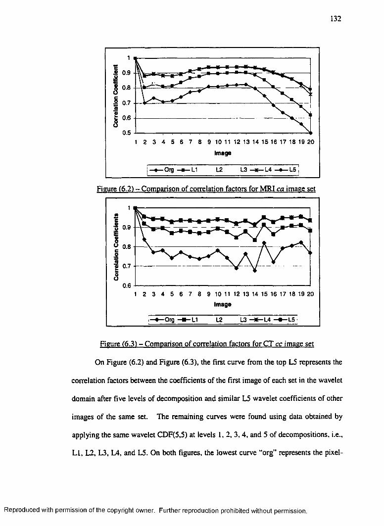
132
JS 0.9
0.8
5 0.7
0.6
0.5
Im age
Org L4
Figure (6.2) - Comparison of correlation factors for MRI ca image set
0.9
° 0.8
e 0.7
0.6
Im age
Org L3 - * - L 4 L5
Figure (6.3) - Comparison of correlation factors for CT cc image set
On Figure (6.2) and Figure (6.3), the first curve from the top L5 represents the
correlation factors between the coefficients of the first image of each set in the wavelet
domain after five levels of decomposition and similar L5 wavelet coefficients of other
images of the same set. The remaining curves were found using data obtained by
applying the same wavelet CDF(5,5) at levels 1, 2, 3, 4, and 5 of decompositions, i.e.,
LI, L2, L3, L4, and L5. On both figures, the lowest curve “org” represents the pixel-
Reproduced with permission of the copyright owner. Further reproduction prohibited without permission.

133
based correlation between the first image of the set and other images of the set. It can
be observed that L5 resulted in the highest correlation, and the lowest correlations
were obtained with the original images. It is also evident that for this set of images,
the worst biorthogonal wavelet curve LI resulted in a better correlation than that
between original images. Also, observed on these figures is the higher correlation
factors resulted with the higher decomposition levels.
d) Wavelet coefficients at higher levels of decomposition of similar images appear to
be more correlated than those at the lower levels. This means that it is more efficient
to predict the wavelet expansion of an image from the wavelet expansion of another
image at the higher levels of decomposition. The effect of the level of decomposition
is less significant when going from level 4 to level 5. This is even more significant
between levels 5 and 6. Thus, for this set of images, 5th level decomposition is
reasonable for image prediction.
6.4 Image Prediction Using Linear Regression
For image prediction, the correlation matrices for the image sets were
computed to determine the linear relationships between these images. Some of the
correlation matrices are shown on Table (6-1) through Table (6-12). The main idea is
to predict any missing or removed image(s) from the set using other images of the
same set. The correlation matrix for the images and the wavelet coefficients obtained
with the CDF(5,5) at level 5 are presented in Table (6-6) and Table (6-12) for the MRI
and CT sets respectively. The CDF(5,5) at decomposition level 5, had in the best
result. Table (6-1) and Table (6-7) present the correlation matrices of the MRI and CT
images respectively.
Reproduced with permission of the copyright owner. Further reproduction prohibited without permission.

Table
(6
-1)
- Co
rrela
tion
matr
ix for
the
ca M
RI-
set
134
05>—8
oin
inCM
00inCM
COCMCM
COCM
opCM
0505CM
00CMcq
p icq
pCOcq
COp .cq
CMPcq
CM00cq
CO00cq
o05cq
CMCOcq
COCOcq
pCMcq
CMT“cq -
00
8
COioin
00CM
CMinCM
CO05CM
inCMcq
05CMcq
Incq
COmcq
COo•or
p .op
o
S
05o■o;
pop
COop
COop
COCOcq
0005cq
opcq -
CMcq
P
8
CO05in
oCMCO
in
3O)
3
05 00T*"CO
05incq
cScq
CO■M
o■O’p ;
p »CMo ;
COpr
CMOP
CO05cq
pCMP
CMpcq
▼—os
pCMCO
<o
8
CDeoCD
COCOp
COmp
©CO
8cq
incq
CO
3
p
3PCOp
inCOp
p«.5
po■p
05cq
COinp
COPcq -
CMPcq
CO05cq
COCOcq
>o
8
CO00cq
o00in
opin
r—CO CO
pCOCO
05PCO
COCOcq
oCOCMM
pCMp
00oTP
pp
0500p
CO05cq -
COpcq
pCMP
COCOcq
CMCOcq
*«•*8
oinP
CO
3—
cqCOCOin
COCOin
00oin
00PP
COp ;
2JGO OPP
inp .p
0505P
tin
CMCMP
T—CO05cq
COinp
CO05cq
COop
o05cq
CO*«•*8
p05P
oo>
pinin
CO05in
05r*cq
pO)in
Ps
ocq
8cq
CO00in
CO05in
o■O’cq -
CM 0500p
05cq
8p
COop
CO00cq
<M**•8
pCMCO
tn CO00p
ooin
CO05in
r~COcq
op .
pCMp
oi t
COCOP ;
COi t
00CM00 - CO
P ;tin
pp
pop
00 1F-P
pop
CM00cq
8
CMCMCO
sP
05inp
oinp
COoin
COCMcq
05P
pCOp
8CO
COCOCO
CO05aq -
00CMCO
ocS
0505p
00op
pp
PCMP
05OP
CMpcq
ca10 00
5PCMp
COp ;
oCOo ;
00pp
■O’pm
8COCMCO i
CO05 -
CO0500
COi t
CO05in
inpp
pCMp
inCOp
OPP
oCMP
COpcq
88
Ooq
inCMp .
05COp
pr-P
sM
COinin s
COMCO
05CO05 -
T—CO05
COCO00
COCOp .
COCOin p
COCMp
8p
PCOp
Pop
pCOcq
§8
CMCO
COCOp
CO5
CMP
PinM
COCOin
op
05CO -
05CO05 £
COCO
«
oi t
CMocq
CM00P
8p .
pp
CMCMP
00op
pcq
PO8
COCOp
CMinp
mp
sTP
COCOp
inCOin
sp . - 05
cqCO3
COCM00
sP-.
pocq
COp
COCOcq
pcScq
COincq
COCMcq
§8
pp_
©pinP
COin
COCOin
pinp -
opp
op i
Scq §
05 — P
r—op .
pcq
00pp
05cq
COpcq
05incq
incq
0505CM
ca05 CO
PP
p5
p00P
pCMcq
r -o00 T-
pmp
inCOin
COCOin
COinin
COCMcq
scq
p05in
00oin
acqincq
COcq
05CMcq
opCM
z8
inp
COpp
CMmin
inCOp
T— o00
CO00in
COCOp
p .ino r
pinp
COp .P
COoin
CO05in
05cq
COCOin
np
pCOcq
05ocq
inCMcq
COpCM
88
op
COCOin
o-
in
£
p .CMcq
COT—in
sp
CMP
p . oCOp ;
oin■o;
ooin
0005in
COCDin
00p
p05cq
05pcq
CO05CM
COCMCM
88
M'COp
Sp -
oCMP
8in
00o ;
pin■or
3p
COP ;
05COP
COpp
05in■»p
CO00p in CO
opin
00inp
in
3.
CMmCM
00mCM
58
COoP - cS
pCOCOin
COpp
p
P
T—op
CMin
COCOp
inCM•or
pCMTP •o;
inpp
o05P
COpin
o00in
COCOp
8cq
00CM
mCM
88
-COoP
3p
©p
inP
COi t i t
p .COCOP
CMCO
oCO
0000
CMCM00
pCM00
P05P ;
oinP ;
CO00cq
COCOcq
0005in
00inin
oin
.188
CO8
88
88
s8
88
88
po8
88
88
o>•»8 8
CM
8
COT—8
p
8
«5
8
<oT -8
p
8
CO
8
05
8
Reproduced with permission of the copyright owner. Further reproduction prohibited without permission.
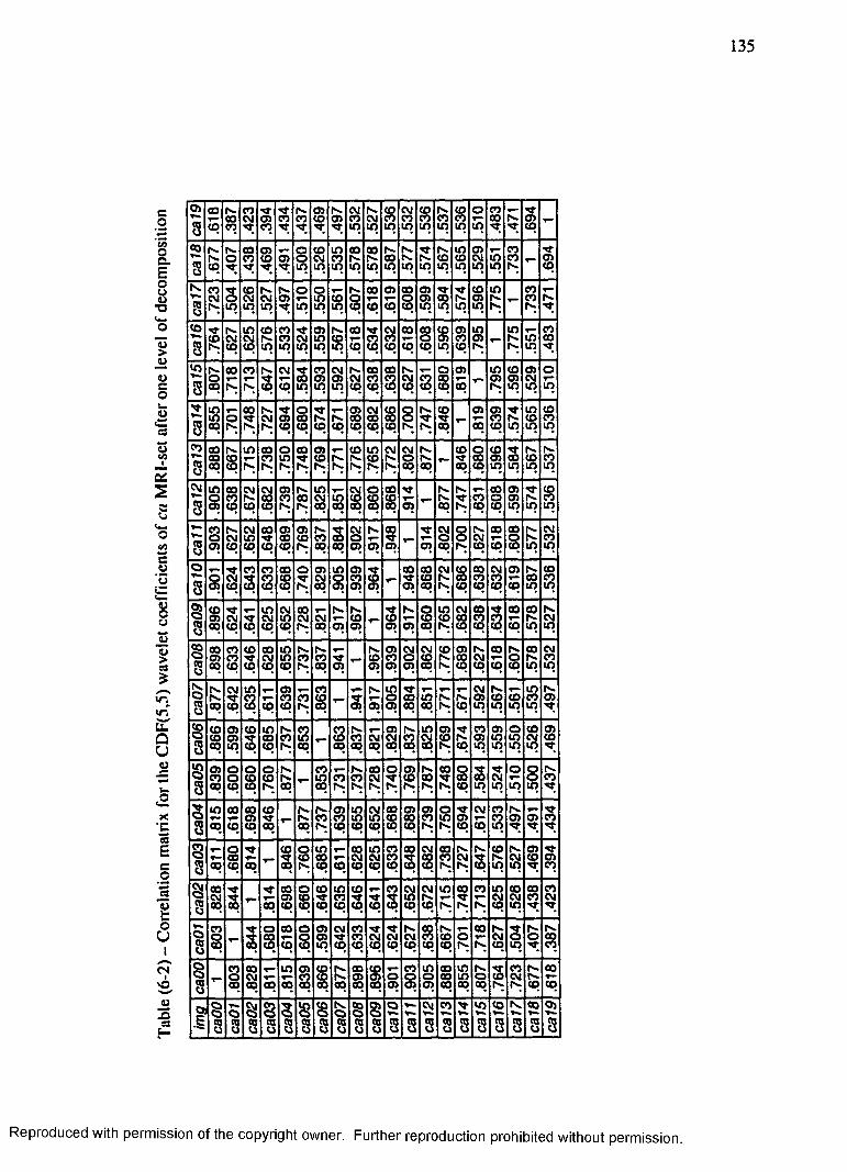
Tabl
e (6
-2)
- Co
rrela
tion
matr
ix for
the
CDF(
5,5)
wav
elet
coe
ffici
ents
of ca
MRI
-set
afte
r on
e lev
el of
deco
mpo
sitio
n
135
OJ 00 IS CO s s rs OJ IS CM IS CO CM CO r s CO o CO ^Ton CM cn CO CO CO OJ CO CM CO eo eo CO CO oo IS OJ
.4 CO CO CO ■s sT M in in in m m in in in O’ COo * * • • * •03 |S oo o> r— o CO in oo 00 i s r s IS in OJ CO
S o CO CO O) o CM CO r s IS OO s r s CO <o CM in eo 1_ OJ8 cq s r ■O’ s • s in in in in in in in in in in IO in IS. cq
IS* CO CO (s. is. o o IS 00 OJ 00 OJ 2 Tf CO in COCM o CM CM o> in CO o o OJ 00 r^ OJ IS T_ eo |S
*4 |s» CO cn CO ■s to in in CO CO CO CO in in in in IS r s• • * •
CO |s cn CO eo M OJ IS oo 3 CM 00 oo CO OJ in in COCO cm CM s . CO CM in CO T“ CO CO T— o OJ CO OJ IS in 00
>4 IS. CO CO O in in in in CO CO CO CO CO in CO IS r s in •To • • * * • * ’|S. CO CO is. CM CO CM IS 00 OO IS o OJ in CO OJ oo S 00 OJ OJ CM CO eo CM CO oo OJ OJ CM T-
8 00 IS. [S. cq cq in in in CO cq cq cq cq cq oq is. in in in
■o- co 00 IS. s f o sT OJ CM CO o IS CO OJ OJ O’ in COcn o CM O) oo i s IS oo 00 00 o O’ CO IS CO CO
8 00 IS. IS. |s- cq cq cq cq cq cq cq rs. rs. oq 00 cq in in in
CO 00 r s CO OO o oo OJ CO in CM CM IS CO o CO O’ r s IS00 CO CO CO ST CO IS r s CO IS o IS 00 OJ 00 CO CO
8 cq cq rs. f s r s is. r s IS. rs. IS. oq 00 00 cq in in in IT)
CNI CO 00 CM CM OJ IS in CM o oo M IS IS 00 OJ ’M’ COo CO rs. OO CO oo CM in CO CO CO r s O’ CO o OJ IS CO
8 Ol cq cq cq is. rs. 00 oq 00 CO 00 OJ cq is. cq cq in in in
CO [s. CM oo OJ OJ r s sT CM IS 00 •O’ CM O IS 00 oo |s CMO CM cn oo CO CO CO O O’ o O CM Y— o |S CO
14 o> CO CO CO CO r s 00 CO OJ OJ OJ OJ 00 is CO CO CO in inO * • * • • • * • • * *o eo CO 00 o OJ in OJ oo oo CM CO 00 CM OJ r s CO
Q CM CO CO s t CM o CO CO •T CO IS 00 CO CO T-* oo CO8 OJ CO cq cq cq i s 00 OJ OJ CJ OJ oq r s cq cq cq cq in in
CO cn CM CO i s i s i s o in CM 00 o r oo oo ISCj O) CM •S' CM in CM CM CO !_ CO CO CO 00 eo CO IS CM8 00 CO cq cq cq rs. 00 OJ CJ OJ OJ 00 rs. cq cq cq CO in in
00 CO CO oo in IS |s rs OJ CM CM CO OJ i s CO r s 00 CMo j o> CO ■s CM in CO CO sT 1_ CO CO o CO IS oo CM o IS CO«4 00 CO CO CO CO r s 00 OJ OJ OJ OJ 00 is CO CO CO CO m ino * • * • * * *
k (s. CM co cn CO r s in r* CM IS m ISo fs. CO CO CO CO 1_ o oo in r s IS OJ CO CO CO OJr4 00 CO CO CO CO IS 00 OJ OJ OJ oo 00 IS CO in in in mCj * * * • * *
5R CO CD CO co rs. CO CO is T“ OJ IS in OJ O’ CO OJ o CO OJCO o j s CO CO in 1_ CO CO CM CM CO CM CO IS OJ in in CM CO
r4 00 CO co CO |S 00 CO CO CO 00 oo oo IS CO in m m inCj * • * * * * • • *o> o o o is. CO r s CO o OJ r s CO o M o o r s
O CO o CO CO rs 1_ m CO CO CM co oo O’ 00 CO CM T- o a8 CO cq cq IS. 00 00 IS. r s r s IS IS is. is. cq in in in in
cn 00 00 CO r s IS OJ in CM CO OJ OJ o CM CO r s y- rtG o j S t __ |S eo CO in in CO CO CO in OJ r—CO OJ OJ CO*4 00 CO CO CO 00 IS CO CO CO CO CO IS i s CO CO in ’M’ -M-u * * • • • * *
o ■s CO o in 00 in CO 00 CM 00 IS IS CO IS OJ ■fl-G CO ( . 5 CO CO CM CM CO 00 CO CM O’ IS CM CO OJ8 cq cq 00 oo rs cq cq cq cq cq cq cq IS. IS cq in in ■*r cq
a CO 00 o CO in CO CO CM CM in CO CO in CO eo COG cm M OJ CO ST CO ■*T t in IS ■O’ CM CM CO CM14 00 00 00 CO CO CO CO CO CO CO CO CO r s IS IS CO tn sT MCj * • • * *
CO — o CO o OJ CM CO O ' O’ IS 00 r s OO r s 2 i s r so o l_ CO o OJ ■O' CO CM CM CM CO CO o T1- CM o O 00{4 CO CO CO CO m CO CO CO CO CO CO CO IS r s CO in T eoCj • * * * * • • ’ •£> CO oo to o j CO IS 00 CO CO in oo in IS ^T CO i s 00G T _ o CM CO CO IS OJ OJ o o o oo in o CO CM i s T*8 00 oq 00 00 00 00 CO 00 00 OJ OJ OJ oq cq 00 fs. IS cq CO
CJ T . CM CO in CO IS 03 o> Q CM co O’ MJ CO IS 00 osS J o o e> CJ o o o o o o s .
.§ cn cn cn cn in cn CM cn m cn ns cn so cn JO jo SO S°u o cl o CJ 0 6 CJ CJ CJ CJ CJ o u CJ CJ CJ o CJ Cj
Reproduced with permission of the copyright owner. Further reproduction prohibited without permission.
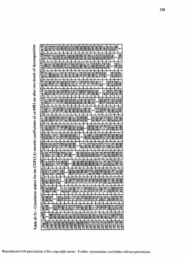
Table
(6
-3)
- Co
rrela
tion
matr
ix for
the
CDF(
5,5)
wav
elet
coe
ffici
ents
of ca
MRI
-set
afte
r tw
o lev
els
of de
com
posi
tion
136
05
s
i ni nc q
c n?
0 0f v
c ni nTT
0 50 0•M;
S i0 5■M;
CMCMi n
c nmi n
CO0 0i n
CM0 0i n
0 50 0in
i n0 0i n
o0 5in
o0 5i n
0 00 0i n
3i n
t vc ni n
3i n
o oc nIV -
ca18 c o
£c nIV c n
oi n
CMc ni n
0 5-M-i n
r vmi n
CM0 0in
-M-0 5i n
COc nc q
COc nc q
3c q
c nc q
re nc q
•M-CMCO
c nCMc q
CM0 5i n
oCMc q 0 0IV t —
0 0c nt v
8
( 0CO1 ";
CMIVi n
0 5i n
0 00 5i n
0 5COi n
0 5 c nc q
COCMc q
oIVCO
oo oc q
5c q
Vc q
c nCOc q
o■ nc q
t vTTc q
3c q
0 5CMc q - 3IV
r »c ni n
< o
8
CMCO
0 0COc q
T—0 5c q
i nc q
oc q
3c q
•m -c nc q
in3
0 5c q
3IVc not v
o0 5c q
3c q
0 5t vc q
i nCMt v
oi nCD -
0 5CMCD
OCMc q
t vc ni n
« n
8
e omc o
0 5COIV
or vV
COr v
CM0 0CO
CMCOc q
■M"c q
0 5
6 f v0 5f v
0 5f v
CMf v
oCMtv COt v
IVo o -
oi nc o
•O ’r vc q
CM0 5i n
3i n
•m -
8
t vCT>o q
i nCOt v
CMO0 0
CM0 0t v
i ni nt v
0 03
IVr v 3|V
c nIVv
0 0COt v
o|vV
CM0 0IV S i
0 0CM0 50 0 - 0 0
i nCM|V
tvTTc q
c nCMc q
o o0 0i n
ca13 CM
c not v
0 5|vV
0 5t v
i n0 5IV
oo0 0
CMCM0 0
3CO 3
3o q
O3
CMCO0 0
CM0 5 -
CM0 50 0
CO|V0 5
6
oi nc q
■m-CMc q
©0 5i n
ca12 o
c nC 5 £
i n■*rt v
i nmt v
0 50 0r v
IVCM0 0
oCO0 0
o0 50 0
CMo0 5
o0 5
COo0 5
c n0 5 -
CM3
CMCM0 0
oCMt v 3
c qc nCOc q
r—c nc q
o0 5i n
8
COCM0 5
0 00 5c q
0 0CMt v
0 5CMt v
i nm|v
i nCO
COCOo q
t vo0 5
c nCM0 5
COc n0 5
0 0i n0 5 - c n
0 5CMCO0 0
CMo oIV
CMT“(V
o0 5c q
3c qc nc q
mo oi n
ca10 i n
S I0 5i n< 5CO
OCMt v
0 0r v
CMM -IV
CO
£
c nCOCO
CMCM0 5
IVT f0 5
CO0 5 -
0 0i n0 5
COo0 5
O3
oIVt v
0 5f v
c not v
3c q
'T3 .
0 50 0i n
§8
CMS i0 5
t v0 5c q
0 5r v r v
0 5CMr v
0 0
£
COino q
Oc n0 5
£0 5 -
IVCO0 5
COc n0 5
o0 5
3c q
0 0COt v
0 5f v 3IV
o0 0c q
COc nc q
CM0 0i n
ca08 CD
S i0 5i not v
-M-CM|v
c nf v
c nc n|V
mS
COCOo q
0 5TT0 5 - f ^
0 5t vTT0 5
c nCM0 5
CMO0 5 3
c nr v|V f v 3
c qoIVc q
COc nc q
COo oi n
r vo8
mo0 5
•<rf v
e n3
0 00 5c q
0 0? v
t v0 0t v
i no oo q -
0 5TT0 5
oc n0 5
CMCM0 5
t vo0 5
o0 50 0
30 0
i nIV
0 5t vc q
i nc q
COCMc q
-M-0 5i n
c ni ni n
88
0 5o q
CMIVc q
t vf v
i nmt v
CO0 5t v
o0 00 0 -
ino o0 0
COCO0 0
COi nc q
c nCOCO
COCO° o
OCOo q
CMCM0 0
i vt v
m -CO
•* rc nc q
c nCO
CM0 0i n
CMCMi n
§8
ot vo q
t vc q
CMc nt v
r v0 0
O0 5 -
oOO0 0
IV0 0t v
i n0 5t v
0 00 0t v
CO0 5IV
i nCD
tvCM0 0
oo0 0
o oIV
CMCOCC
TToc q
0 5t vi n
t v■ ni n
CM0 5'T
38
i n° o
m00c q
t vi nt v
IVr vc q - o
0 5CO0 5IV
00f v
c nc n|V
0 5CMt v
CMt v
i ninIV
0 5o oIV
i n0 5t v
i nmi v
CMCOc q
oc q
0 5COi n
0 5TTi n
0 5o o
88
CMmc q
0 5c nIV
oi n00 -
t vf vc q
tv00
i nmr v
000 5c q
c n£ f v
0 0f v
0 5CMt v
i nintv 3r v
S i0 0t vCOf v
3c q
0 00 5i n
CMc ni n
c ni n
88
COc no q
ot v0 0 -
oi n0 0
t vi nIV
CMc nIV
t vr v
c ni v
CMt v0 5f v
OS i
CDCMIV
int v
0 5IVIV 3
oo.ot vt v
3c q
0 5i n
c noi n
o oIV*ar
o8
COc nc q -
ot vCO
0 5c nt v
i n00c q
■<rIVc q
CMIVCO 3
i nor v
IV0 5c q
i n0 5c q
o o0 5CO f v
OTTt v
i nCOIV
0 5COIV
COCDc q
CMIVi n
c nIV■M;
c nM 'TT
§8 -
COc noq
c nCO00
CMi nc q
i n00o 0 5
oqt no0 5
c nCM05
CMCM05
mS i0 5
COS i0 5
Oc n0 5
r~CM0 5
IV0 5oq
c ni noq
CM00
COCOf v
COf v
i ni nc q
I §8
^— o2
S i8
§8
32
88
35
t vCO8
38
32
O
8IV8
CM
8c n
8■o-
8i n
8CO
2t v
80 0Y«*8
0 5
8
Reproduced with permission of the copyright owner. Further reproduction prohibited without permission.

Table
(6
-4)
- Co
rrela
tion
matr
ix for
the
CDF(
5,5)
wav
elet
coe
ffici
ents
of ca
MRI
- se
t af
ter t
hree
levels
of
deco
mpo
sitio
n
137
o j
5 .69
7
.50
5
.53
9 COY“in 54
2.5
45 CM
rxin .6
03
.63
5
.63
2
.63
9
.63
6 CMXTcq
CM
cq
CM
cS
oCMcq
o
cq .62
2
.79
8
Y-
00 CM oo OJ 00 CO xT 00 IX IX XT IX CO CM CO CM CM CO ooCO x r rx OJ o Y— CT XT 00 00 OJ 00 oo 00 00 IX CT OJ
w |x CO in in CO CO CO CO CO CO CO CO CO CO CO CO IX 00 IXo * * * *
|x 00 o XT OJ CO 00 00 CO 00 o IX T CT CT o CO CMM- |Xx |x . x r xT IX 00 CM CT CT CT CM CM CT CO rx 1_ CT CM
8 cq cq cq cq cq cq c q c q |x . tx IX. |X IX. IX IX. IX. oq 00 cq
co CO in rx OJ XT 00 o OJ 00 OJ Y- in Y- CT o CM oCO xt in CM 00 00 o CM in CO c o CO co CO o 00 IX 7—
8 CO fx. |x . |x- cq c q |x . IX IX rx rx rx. IX. IX. 00 CO 00 IX cq
in in 00 CO in 00 00 XT o 00 oo 00 in CT CT CM ocn o IX M CT xT in 00 OJ OJ 00 OJ CM OJ _ 00 CO |x CM
8cq 00 00 IX IX. |x . IX. rx rx IX. rx. IX IX 00 00 00 IX. cq cq
xt CO rx IX v— in O CM o CO OJ 00 CO 00 in CT CO CMCM o eo OJ cn O Y - CT CM CM CT CO o Y_ OJ o CT oo TOJ 00 00 00 |x |X 00 00 00 00 00 oo 00 OJ 00 00 IX CO CO
u * * • * • * * • • * * *
CO (X OJ oo CO OJ CO OJ in CT 00 CM s OJ 00 00 in XT CM CMCO 00 r* CM T~ CM CO fx CO IX 00 o CM CO CM oo XT
8 OJ N co CO oo 00 oo 00 cq 00 00 00 OJ OJ 00. IX. IX cq cq
CM CM CO •O' M- CO 00 xT o CM CM ■M' CO OJ CO 00 Y- IX CO CMCO OJ OJ x f IX o Y* CT CO OJ c o CM oo xgr
o> |X rx. IX 00 oq 00 OJ OJ OJ OJ OJ OJ °o IX IX. tx . cq cq
cn OJ s O |x in 00 CM CO CO oo CO XT oo 00 Y- o IX COCO in 00 00 OO CT fx CM CT in CT 00 CT 00 co CT oo CT
8 o> |X |x . IX IX. 00 00 OJ OJ CJ_ OJ OJ oq 00 |X» fx rx cq cq
o OJ in 00 M' o in CO OJ 00 00 XT CM OJ OJ oo XT OJCO in rx IX oo CM IX CM xT CO in IX CM OJ CO CT OJ CT
!4 cn rx IX. |X IX 00 00 OJ OJ OJ OJ OJ 00 oo rx rx rx CO COVJ • • * * * * * • • • • • •
CO CO CO OJ OJ CT T“ 00 CO CM 00 CO o 00 CO IX CMO eo in rx CO rx CO CT |x Y» CO CT Y— CO CM OJ CO CT 00 CT
OJ rx rx IX IX 00 00 OJ OJ OJ OJ OJ 00 00 IX IX IX CO COO * * • • • • * *
8 (X. CM Y- CM x f OJ rx o Y_ OJ CO CM CT o OJ oo IX inqa CO CO 00 rx IX rx in __ rx XT CM Y— IX CT 00 in CM 00 CTr4 OJ IX. rx rx 00 00 OJ OJ OJ OJ OJ oo oo IX rx rx CO COvJ * * • * * * * * * *
CO CM oo o CM in o CT CO CM o in CM 00 o CO oo CTO CM rx rx. in CO OJ ^_ in CT CM o CO Y- in CM oo T o8 OJ rx. IX. IX. IX 00 oq OJ OJ OJ OJ OJ 00 00 IX rx. c q cq cq
8 CO in y » o OJ OJ in IX OJ in oo XT OJ Q CO 00 CO XT CMw O CO rx. o OO . OJ IX CO IX IX IX XT o XT o tx CT IX8 OJ r x IX. oq 00 cq c q cq 00 00 00 00 oq 00 rx. IX. c q cq in
|x CM xT OJ OJ CM OJ XT o in 00 CO in XT OJ Y- inO CO CO oo M 1 o 1_ 00 CM CT XT CM OJ CT 00 XT Y-r 4 CO r - rx. OO OJ 00 00 00 00 00 00 00 00 IX fx CO CO CO inU • • *
s CO CO ct OJ OJ o XT IX CO OJ Y u j OJ 3 CO CM|X eo CJJ OJ o Y— CO rx rx 00 00 OJ XT 00 xT o
8 c q rx (X. 00 OJ 00. IX. IX. IX. IX. IX CO 00 IX IX. c q c q c q in
OJ CM CM « xT o 00 CM OJ • ^ o XT CT rx CO IX Y_ CO COO fx 00 IX. OJ o in IX CO IX 00 OJ CM v— IX CM IX OJr 4 CO r - 00 00 00 00 IX IX IX r x IX IX 00 00 rx IX CO in inU • • * * •
OJ CM CO Y“ Y - CM CO 00 < r XT 00 IX XT in o OJ OJo CO 00 IX. cn 00 IX IX 00 rx IX 00 cn CT in |X IX CT8 00 00 CO |x . rx. IX. IX IX. rx IX. IX IX. oq cq 00 IX. cq in in
T»* oo c r CM CO CM in CT CM CO in OJ oo OJ n CO CO oo 00 inQ CO oo OO CO CT CT rx CO in in in CO oo o o XT xT o8 oq cq |x IX. rx. rx. rx. IX. IX. IX. px rx. IX. oq oo rx c q in UJ
s> 00 cn OJ Y~ rx CO f x CO OJ OJ CM rx XT in IX CM IXCj CO 00 IX IX 00 o CM CT CT CT CT XT CT CM OJ CO CO O J8
00 oq 00 00 c q OJ OJ OJ OJ OJ OJ OJ O J OJ oq 00 CO IX. c q
o Tx Sit cn in CO rx QQ OJ © Y~ CM CT XT VJ CO IX CO OJs CJ c s CS o o CS o CS CS o X X »— X . Y* X£ CQ CQ CQ CQ CQ CQ CQ CQ CQ CQ CQ f® CQ f® J® CQ s® <0 J ® 5®CJ CJ CJ o CJ CJ CJ CJ CJ o CJ CJ CJ o CJ CJ o CJ o
Reproduced with permission of the copyright owner. Further reproduction prohibited without permission.

Tabl
e (6
-5)
- Co
rrela
tion
matr
ix
for t
he CD
F(5,
5) w
avel
et c
oeffi
cien
ts of
ca M
RI-s
et a
fter
four
lev
els o
f de
com
posi
tion
138
o>
8
OJinrx
oOJin
OJ
cq
x fOJin
CM
cq
CM
cq
COeocq
OJincq
0000cq
IX00cq .6
93 OJcq .6
98.7
03 CM£ .7
08 OJorx
x r
r ^ 00 -
eo OJ OJ on o CM in CO o CM CM OJ CO OJ CO CM o o CO x rCO CO rx rx rx OJ x r xT x r x r x r m CO in IX in CO
8 CO cq cq cq cq cq cq IX. IX. IX. |X rx |X IX IX |X |x oq cq
N . T“ CM x r CO rx CM O O m OJ in CO CO CO 00 O CO x rCO CO CM o o eo in 00 CO OO 00 CO CO 00 OJ ao y y inCO rx |x . rx IX rx IX rx rx |X IX rx |x IX rx |X 00 00 rx
vJ * * * * • * • *CO rx OJ CO XT OJ OJ o CO OO CM O OJ OJ rx o o OJ
00 fx . oo in CO CM m CO o o o O o OJ 00 00 IX o8 00 fx. |x . N . rx |X tx rx oq cq 00 CO 00 IX 00 co oq IX IX
«o tx eo IX. CO in CO IX IX o CO in O CO in x r IX 00 O 00o CM CM OJ rx CO IX CO T- CO OJ 00 OJ m o
8 OJ 00 00 IX rx. rx. IX IX. 00 co 00 00 ao oq 00 CO rx IX IX
x r rx CO CM OJ CM x r x f rx CM in s in x r OJ CO CM CMCM t— x r CO o ▼— CM CO CO CO xT CO o 1__ OJ ao CO
8 OJ °q 00 00 00 00 oq ao oq oq 00 00 oq OJ cq cq tx IX rx
00 ix 00 CO CO eo in s in in OJ CM CO in in cn CO CO COCO cn CM CO eo CO in CO rx CO CO CO T— o eo OJ 00 lO o
8 OJ tx. oo 00 oq oq oq cq 00 00 cq CO OJ OJ 00 IX rx IX IX
cvi CO x r T . CO in 00 OJ 00 00 r~ x r CO CO o CO OJ 00XT oo cb o CM in rx OJ o o ▼— cn CO T - o 00 x r OJ
8 OJ rx. 00 00 00 00 00 oq OJ OJ OJ. OJ OJ 00 co 00 tx IX cq
CM CO tx. CO IX X t x r in |x s CM y - o CM in CO y -
xT 00 OJ 00 OJ oo CM CO m CO 00 x r t— o 00 x r OJ8 OJ rx. IX. rx. rx oq oq OJ OJ OJ OJ OJ cq 00 °q 00 rx rx cq
o CM CM CM CO IX 00 OJ rx rx OJ m in 00 OJ OJ COS 00 OJ 00 OJ CM rx CM x r CO in T“ 59 CO .— o 00 x r OJ
8 OJ IX. |x . IX. IX 00 00 OJ OJ OJ OJ OJ CO 00 00 00 IX tx cq
OJ rx © T* S rx in 00 in CM CO CO in CM rxCj CO oo OJ IX 00 CM IX CO rx CO eo o CO CO T - o 00 XT 008 OJ rx. rx. IX. IX. 00 00 OJ OJ OJ OJ OJ 00 00 00 CO rx rx cq
o CO in o CO CO o o T“ OJ x r CO IX o o o CM ooO x r 00 OJ 00 CO CM 00 m IX x r CM o IX CO T - o ao x r 00OJ rx. |x IX |x 00 oo OJ OJ OJ OJ OJ CO ao ao 00 rx IX COu ’ • * • • • • *
K . IX CM rx S x r CM o x r oo x r OJ m OJ o o OJO CM OJ 00 rx IX CM o in CO CM r - OJ CO CM 00 CO in y— in8 OJ rx. ix . IX. IX. 00 OJ OJ OJ OJ OJ 00 oq oo IX IX rx IX cq
CO CM m co in ■O’ CM o y— rx r — oo x r |x y - CM CO eoW CO 00 o CM OJ 1_ O 00 IX rx 00 rx in rx in eo OJ eot\ OJ rx rx oo CO 00 OJ oo ao ao ao 00 00 oo rx rx rx CO COVJ * * * * * * * •
in 00 eo in CO x t x r CO o CO y - in m CM CO OJ |x m CMo OJ in OJ o OJ CM CM CM CM in CO CO CM o r x T *8 00 fx. tx . oq OJ CO 00 00 CO 00 t o oq oq cq rx |x IX cq cq
o in in x r CO |X CO CO OJ in x r CO CM CMO oo CO OJ 1__ o CM rx oo OO OJ OJ CM eo o IX eo o rx T*00 IX. 00 00 OJ oo |X IX IX IX |x oo CO 00 |X rx IX CO COu * * * • * • • *■ • •
p in OJ IX in in CO o |x CM CO y - CO CM CO CO o XTO oo OJ rx 1__ OJ XT o IX CO IX 00 ao o eo CO OJ m CM rx OJ8 00 |x . oq 00 00 cq IX. rx. IX. |X rx 00 aq 00 IX IX IX cq in
IX cn rx o eo in IX m CM rx x r CO CO rx y - ao OJCj OJ oo (_ rx OJ oo ao OJ OJ OJ OJ o CM x r CM ao co COW 00 00 00 00 rx IX rx rx rx IX rx 00 00 00 ao rx rx CO COVJ * * * * * * * *
CO CO OJ oo CM CM CO CO x r 00 eo OJ CM OJ oCj CO r 00 OJ CO in CO OJ CO 00 ao ao 00 OJ CM rx T~ co OJ8 oq oq IX. rx rx ix. IX rx IX IX rx rx IX 00 00 fx IX cq in
?! eo |x in l_ in CO rx o OJ CM CM eo rx rx rx rx OJ OJx> 00 OJ oo oo OJ CM x r CO v x r x r CO CM o 00 COoo 00 CO 00 CO OJ OJ OJ OJ OJ OJ OJ OJ OJ OJ oo CO COu * ’ * ■ ■ o
CJ Tx CM co IT) £ rx 55 OJ o Tx CVl CO x r •n CO rx CO OJ2 CJ CJ CJ o Cj O 5 o o Xx Tx Tx Tx Tx Tx Tx Tx TX Tx
F m m cn co cn cn cn cn cn cn cn cn cn cn S* 50 5° cn focj Cj 0 CJ CJ o ci o CJ CJ CJ CJ CJ CJ CJ CJ CJ CJ CJ CJ
Reproduced with permission of the copyright owner. Further reproduction prohibited without permission.

Tabl
e (6
-6) -
Corre
latio
n m
atrix
for t
he CD
F(5,
5) w
avel
et c
oeffi
cien
ts of
ca M
RI-s
et a
fter
five
levels
of
deco
mpo
sitio
n
139
ca19
1CM05P-;
oCOcq COcq 5cq
05incq 8cqCOCOcq
CO05cq CM
P-.
oCM|v
p -CMp .
in53Pv
mCOPv
COCO|v .
CO CO
£p .oPv
COCMCO -
00s
pvCMCO
3cq05r-cq
05Is-cq
COCOcq
o05cqCOf -
mp-.
ininp-.
ininPv
CMCOIV
inPv
05inPv
CO|v
inCOPv
inR
ininPv
COr rcq -
COCMcq
P -
8
COin°qrv
£COCMr-;
COIV.
sr05cqCMoP*;
inCOp -
COinPv
05p -|v
spv
CO00Pv
CO|v
COIV
COp -Pv
COp -p -
CMCOp -
05CO00 - CO
00P -o|v
<o8
oCOcq
CM
s05Is-IV.
05■M"P-
mS.
COCMP-
05•O’P-
COCOr-
CO05P -
0505P-;
0505Pv
c*d05p -
0500Pv
COCOp -
oCO
mIV00 -
05COcq
inm|v
CO
£V)V—8
CMo05
inCMcq
Is-CMCO
05|v-CMIVP -
oCOPv
COP-P -
00p -
0505Pv
COocq 3000505tv
Y-ocqcoCMCO
inCOcq - in
PvcqCMpv
in|v
00CM|v
■o-8
CMCM05
o00
CO■cCO
COCOCO
O00
p -
805ocq
cor~~eoCOCMCO
CMcq CM00CMCOcq
mincqCO05CO T*in
COcqTto00
COPvP-;
inCOtv
00CO|v
CO
8305
CO05P -
CMCM00
COCOcq
05COCO
3cqCMinCO
!ncq scqinincq
oCO00
■M-P -CO
o05 -
CO0500COCM00
COCOp
COPvpv
COPv
inCOrv
CM
8505
OCO|V
0505(V;
oocqoCOcq
P-incq05IVCO
in05cqCMo05
805
in§>
oCO05 -
o05
inincqr—oCO
05COpv
aPv
05inPv
COpv
*•>»8
O05
00rvp -
05p -
CMCOIV.
p -05IV
CO
3 COcqCM05
oCM05
CO05
305
T—oCO05
■<PP -00
CMCOcq
0505pv
CO05P-.
T—COp^
p»in|v
inCMP>;
calO o
05inIs-rv s
Is-.
COrv(v.
O05P-.
COCMcq
05rvcqPv
§>CO05
COCO05 T“
Tfin05 805oCOcq
'pCMcq §00
0505P-
COCO|V
CMCOPv
PvCMPv
ca09 p -
CO05
inp -p -
COCO|v.
COPvP-
5Pv
KCO
COp -co 305
©Pv05 - CO
CO05
5305 105
inincq CM00COo00
0505pv
sIV
inmPv
oCMpv.
ca08 CO
CO05r -p -Is-
in00Pv
mrv|v
eoCO|v
COCMcq 5cq
00■<r05 T“
opv05
COV05
oCM05 805 COcq
COCMco
0505IV
CO05Pv
05rvpv
ininPv
CM|v
P -Q
8|vCM05
os
p»Is-r -
p -cop -
inP-Pv
inCMcq o05 -
0005
CO05
P-CM05
CM05
in05cqP-tncq
COao 5
PvCOCOPv
COin|V
i—COrv
CO05cq
§8
inO)
8Is-
RIs-
0005P-
COCMcq 0500 Y - O
05CO00
COCO
05PvCO
300 RcqCMinCO
05ocqCOPvPv
05■M-Pv
inCOP»
CO
£COCOCO.
§8
05CO
Is-
R05Is-|v.
oCOco
oo05 r — 05CO
inCMcq
COCMCO §
COCM°q
CO
CO
p -mcqTPCO00
P-OcqOS
COCMPv
CMopv
o05cqoCOcq
58 CO
COinIs-
OoCO
inCO00 - OO05
COCMCO
inP -p -
COCOpv
Y—00pv
O05IV
IV05Pv
oCOcq
05CO00
oCO
CMPvPv
inCMp-.
Tf<5cqCOCOcq
05inCO.
§8
xf00CO
'*•05P-COIs-co- ■n00cq
OCOco
CO05P -
P-coPv
inp -pv Rpv
COPvIV
CMCOP-.
oocqCOCOCO
COCO00
SP05Pv
05u-|v
COr-
05Pvcq cq
£8
■*r05CO
CMCOCO
T- COPvcq
oo0005PvPv Rpv
IVr -Pv
inCO|V
CO
sTTCOPv
05rv0505P -
CMCMCO
COcq
P -CMCO
05Pvpv
COCMp -
05pvCO
CMCOcq
o8 CO
CO -CMCOCO
05P -
inIV
P -
RCMin|v
oCO|v
IVp -r v
inP -p -
inPvp -
COpvrv
oR
CO05Pv
oCO
inCMcq
CMCOPV
p -
p -Mincq
oCOcq
§8 -
r—CO00
Tf05CO
COCO
COcq G>00in05
P -CM05
00CO05
P -CO05
o05
o■M"05 §>
VCO05
CMSI05CMo05
OCOcq
COincqr -CMcq
CM05Pv
S 88
>-o8
88
88
88
88
88
IVO8
88
§8
O—8
V -
8CM
8COV—8
■M-8
in ——
8co8
p -T—8
ao8
058
Reproduced with permission of the copyright owner. Further reproduction prohibited without permission.

Tabl
e (6
-7)
- Co
rrela
tion
matr
ix for
the
CDF(
5,5)
wav
elet
coe
ffici
ents
of the
fir
st 20
imag
es
of the
cc
CT-
set
140
058
aoCOIs*; V CMrv
05rv
oCOrv05O00
CO05rvy05rv
00orvIVin|v
0505IV(VCO|V
05o0000 cyo00
o 00IV|vCO|vv
cy05|V -00 COCOy c\r CM CO00 o 05 05 cy 00 cy in cy cyCMy T*" COr—V CO V s cy *—cy cy y cy 05 T_ 05b 00 00 00 00 IV 00 rv rv 00 r rv IV 00 rv 00 IV00 00 IV
in y o oo 05 o rv IV o o COcy o 00 O 05 cy COo o 00 oo CO00 00 00 COV m cy 05 COo V 05 05 V%00 00 rv rv rv rv rv rv rv rv rv IVrv cq 00 |v IV 00 rv<o cy 05 CMCO00 COo 05 CMin 05 cy y. Y“ rv 05 in 00o> *—00 o CMV COCO00 05 V cy CO05 00 cy 05 cy Vb |V 00 tv 00 |V rv rv rv rv rv tv IVrv cq rv IV |v ao rvV) 05 IV CMCOIV 00 m COO CO05 in |v o cy oCMCOCMCO V y in COo COCMcy COCOn cy V y yb |v |v tv IV|v rv tv rv rv rv rv |V i". cq rv rv IViv |Vy o> y CMCOy CM05 (Vrv 05 in o y 05 IV IVCO00 cylO V oo 00 05 V m 05 CO05 IV in ao o St ob 00 00 IV V rv rv rv V IVrv rv rv 00 co IVIV00 00 oo* * * • • • • • • • * *05 COCMCMCMCO00 o 05 00 CO05 cy rv 05 in o cy ooIVo O IVy CO00 00 COCO05 o o IVCO05 COcy y& cq rv rv cq cq IVcq cq cq cq IVrv IV cq cq COcq rv rvcy 00 rv COCVI rv 00 m o CO05 ■« y IVy 05 y- cy 05 05COin m rv V rv 05 IV00 in 05 o y—COco 05 ▼—ob rv IVIV rv V 00 rv rv rv rv rv rv |V ao IVtv IV00 00* • * * • * * • • • * * * * *
00 in O) © COCO COo y o y cy o COcy ao 05 rv00 CMrv rv COCMin 00 CO05 in 05 o 05 cy cy cy cy COb cq rv cq cq tv iv IV rv cq cq rv IVrv rv IVrv rv rv tv
CM00 CMCOy in 05 COCMrv o y 05 in o 05 o CO05y in COCMy in rv 00 y 05 y_ m in 05 COcy rv in co 05b Iv rv rv rv rv tv rv IV tv tv rv IV IVtv rv tv |V IVIV
CO05 in oo COCO CO rv y 05 CO05 COm o o IV00 rv rv T—rv 05 00 in y 05 05 00 CO05 CO05 IV |v inb rv IVrv oo rv tv rv IVrv rv cq IV cq IVrv |V |V rv rvs> r- COor rv y COy COcy o CO00 rv in cy IV00 ooin 00 rv 05 CO O y y COIV00 in o 00 COT—ob rv rv 00 rv cq rv IV rv IV rv cq IVcq rv rv rv |v 00 rv
rv in COo y o y 05 05 o 05 tv 00 05 y- 05 yCOy CMto CO o to 00 00 05 COIV CO05 00 CO05b rv rv tv rv 00 rv 00 IVrv tv tv |v cq IVrv rv rv IVrv
$ 00 00 COCMo in O 05 05 y in o 05 IVo rv T* 05y in CMCO CO CO ao IV m rv 00 05 in CO00 rv 05b |V rv IV|V 00 |v 00 |V rv rv rv rv cq IVrv rv rv rv rv
$ CMCOCOCMin in T—COCOin CO00 ao cy COCOo cy 05iv 00 COrv y COCOCO05 in cy CO00 y IVao oiv rv n. rv rv IV rv rv rv IVrv oo rv rv IVrv rv 00 aoVJ * • * * * * *T“ 00 COin in O y y 00 y 05 rv 05 y cy ao 05 cy oy CO00 CO y T* CM05 rv y 05 rv y ao IVcy COSP COrv IVCOrv IV00 00 COIVIVrv IV COrv IVIVrv rv IVVJ ■ • * • • • • • *
S? O oo in CMCMo rv m COo cy cy COy- 05 00 0500 in COy^ COtv CO rv cy rv rv IVIV05 o 00 t—b rv |V rv rv IVIV IV|V 00 rv cq tv COrv IV00 rv cq rv
co oo COCOCOCOCM05 cy 05 05 cy cy rv cy o co cytv 05 1_ 00 oo COCMT“ IV05 rv in o m cy 00 00 y—rv IV rv COrv rv rv 00 rv rv COrv rv IVIVIVrv GOrvu * * * • • * *00 COo oo COCOm 05 05 oo m rv cy y 05 05 y COIVCj CO 05 in CO00 m y COrv m cy m o 05 y—o rv
b 00 IVrv rv IVrv rv rv |V IVtv |V |V 00 rv 00 00 00 rvs> 00 T“ CM00 rv cy ao COCO05 y_ cy in T- 00COrv COy IVy 05 in ao y ao COIVy—cy 05 o CVJ COb 00 rv rv tv tv rv rv rv rv IV cq tv cq 00 rv iv cq GO|V
o CMco y »n CON co 05 O cy 05 y COrv 00 05s o Q Cl o © C5 © C5 C5 o T..5 u u (5 Ci CJ o C5 15 ti o U u p p P P p p po u O u O u o u u o o u u o u u u o o
Reproduced with permission of the copyright owner. Further reproduction prohibited without permission.

Table
(6
-8) -
Corre
latio
n ma
trix
for t
he CD
F(5,
5) w
avel
et c
oeffi
cien
ts of
cc CT
-set
afte
r on
e lev
el of
deco
mpo
sitio
n
141
cc19
1 C O0 00 0t f lo o0 0
mi n0 00 3m0 0
C O| vo q o0 3r v0 30 0
0 00 3c q0 08
C OI VC O 80 3C O0 00 0
0 30 30 0C MS o o0 3 S o
| V0 0G OC OC O0 0
i n0 30 0 -0 0T —
8 0 3C MC M0 3
0 3o0 30 3o0 3
0 0| v° qC Oo0 3
mo o0 0o8 o0 3
mC O0 0C O0 30 0
C MC Oc q 20 3 8c qi n2 &
0 * 32
0 32 -
i n0 3c qi v8
O Oo0 3 20 3C OO )00 §
t v0 0o o0 3C O0 0
oo0 3i n0 3c q
r vo o0 0 S i0 30 00 30 0c o Rc q
t v0 30 00 3C Mc q
0 3o0 30 * 30 3C O O0 3 -
0 32
C OC O0 0
cc16 0 00 30 0
o0 3
C O0 3C O 20 3 C O0 0 2C OC M0 0c q
o0 0 0 30 0 §0 3 S i0 30 0
COCOc q0 0S o
C M8
C O0 3C OCOC OC O -
T “o0 3C O2
| vC O0 0M 38
T fC O0 00 3C Oc q
C M| v0 0 RC O 0 30 0oi vo q
C Oo o0 0o0 3C O 2o q S i0 3c q
0 3C OC OC M C O
8COCO0 0 i -
COCDCO0 * 30 30 0
r -I Vc q Ro q
8C OS i
i vo0 3 C Oo qm0 3c q
C O0 30 0C O8
C Oo0 3 0 3C O R0 0 o0 30 08 s0 0 o0 3
i n0 * 30 0 - 20 0C O0 30 0
0 3O0 3i nT “0 3
T —o0 30 0
8 20 0 i i nc qmC Oc q
• O '0 0
0 3C O
0 3C O0 0C M2
0 0c * >CDco8 S i0 0
i ni nc qC O3 - 8
0 * 30 * 30 0 20 3S i0 0 80 0
C Mr vC O
CC12 0 3f vo q
C Or v0 0C OC O
C OC Oc oi n0 0c q
i no0 3C OC Oc q 2C O i 2C O
C OI Vc qC OC Oc q - C O
2 o0 3C OC O0 0
C O5
I V0 30 0 20 30 30 3C O
8 2 C O0 0T —2
or vc q0 3i n0 0
i nC O0 0C O0 30 0 8Q O 2C O
C O0 0c q - C OC Oc qi ni n0 0 800 §
0 * 30 0 R0 0
C MC OC OC OC OC O
cc10 r0 0
o0 0c q R0 0C M| vC O 5
C O0 0
0 00 3c qC O0 3C O RC O Rc q - C O
8 RC O S i0 0 8c q0 3COCOsi0 3C O
O O00C OC O0 3C O 80 3
§8
0 3C OC OC Oo q
I V0 30 0 0 3 S io >G Om£h •
£C O0 3I VCOR0 0 -
r vI V0 0 2c qT~0 3C O
0 * 3e * 30 0 iC M0 30 0 80 3
C M0 30 0i no oc q
C OS o
II Or vC O
o0 30 0 0 3 0 300 sr va o
i nmc qr v2 , - I V0 0
to( VC O0 3S io q 2o q 8C O sC O 20 0 2o q
I V8
0 3o0 30 08
N .1
q sC Oc qor vo q
oC Oo q0 0i n0 0
i n0 3
i nr vc qi nC O0 3 -
t v2
0 3I V0 00 00 30 0
C O0 3c q 2o q %r-0 3C O
o0 3C OoS o
i n0 3c qo0 00 0
C O0 3o q
cc06 C Or v0 0
C Or v0 0 C Oc q Ro q0 0o0 3
0 0r vc q -i nC O0 3
i ni nC 0t v0 30 0
000 30 0i n8
< oo oo q0 3C O0 0 s0 3
C O0 00 0 8C O 80 3i nC Oc o
I V0 3C O
\cc0
5 C M0 00 0i vC OC O
0 3« §
mC Oc q -C OC O
i nI Vc o Ro qm0 3C O R0 0
0 3i nC Oi no0 3
0 3 0 00 00 0ot vC O i
C O0 0C OC * 3o0 3 o0 3
!0 3C O0 0 2c o I
©r -c q - i nC Oc qC Oo0 3
i n0 3 2 Si0 3° q R0 0
oS o
i no o0 0* r2 8o q 0 30 0
T —C O0 0 80 0S o
C OI VC O
1C O0 3C O
C Oi v0 0 0 3 - oC O 2c q RC O 80 0 § >
■ M -2 S i0 0 2 8C O
i nC OC O 20 30 0 RC O 20 3 o0 30 3o0 3 i n0 0
io0 30 0
0 30 3o q - 1i0 3r v0 0
r vC O0 0 §Q O 0 3t v8 R0 0 2
C Ot vc q 2o q 20 0 £c q 0 3C OC O0 3C O
0 3O0 3i ni no q
1ow0 3 - 0 30 3C O
mr »c q 2C O £0 00 0 RC O
O0 3C O 8COoC O0 0 2C O
COI Vc qr r2
I V8
0 3C Oc qo2
T To0 3C M0 3
i nCOc q
I -o3
o0 30 0C O0 3ao
0 3C Oc qC M0 0C O
C OS o
0 3C OC Oi nI VC O 2o o i
| v 0 3I V0 0 2o qto2 2c q 20 3o q
C Oo0 3 20 * 30 0o q
I IS8 i I 2
8 i 1IV
11!o
8 8C MV *
8C * 3
8 8M 3
8c o
8IV
8Q )
80 3
8
Reproduced with permission of the copyright owner. Further reproduction prohibited without permission.

Table
(6
-9)
- Co
rrela
tion
matr
ix for
the
CDF(
5,5)
wav
elet
coe
ffici
ents
of cc
CT-s
et a
fter
two
levels
of
deco
mpo
sitio
n
142
cc19
\
CMo>
CO05
O05CO
20500
&05
tvCM05 .9
24
.92
6 CM0000
s05
|vCM03
CO05 .9
24
.90
3
.92
6
.90
4 in05
CO05 .9
22
-
00 in 2 CO CO CO CO CO o 2 CO CO 2 fv tv CO CO tv CM CMCO CO CO o CM CM 05 CM 00 CO o CO 2 CM
b 03 05 05 05 05 05 05 05 03 03 05 cq 03 00 05 03 03 05 03
IS. s r CO 05 CO CO CO CO 00 o CO CO CO tv in CO CM COCO CO CM CM CM CM CM o CM CO CO CM CM 2
b 05 05 05 05 05 05 05 05 05 05 05 05 05 cq 05 05 03 03 05
co CO in 2 00 CO CO CO CM 05 2 2 tv fv CO CO CO IV inCM CO CM CM 05 O CM CM 03 O IV CM 05 CM CO T"
b 05 05 05 05 CO 05 05 05 05 05 03 CO 03 oq 05 CO 05 05 05
o CO 05 CO O O T“ in in o CO CO CM CO 2o o o o CM O CM 05 CM o o IV 05 CM o ob 05 05 05 05 05 05 05 05 CO 05 03 05 05 CO 05 CO 05 05 05
2 (s. CM CO CO O in CO O o 05 IV 05 CM s — CO CO in S9 COCO CO CM CM CM CM CM 05 CO fv CM CO CM05 05 05 05 05 05 05 05 05 03 03 00 05 CO 03 03 03 05 05
• * * * * * * *co O CO CM |v CO IV CO 05 in IV o IV fv fv CO
rv rv CO iv in O r s |v IV CO o 05 tv IV iv tv CO CO oH CO CO CO CO CO 05 CO CO 00 CO 03 00 CO 00 CO 00 OO CO 05vj * * *c \| CO CO CO in CO 05 CO IV CO |v IV CM in fv CO IV 2
o o o r—T“ CM CM v— o 05 IV CO y— o CM CM CMb 05 05 03 05 05 05 05 03 05 05 03 cq cq 05 05 03 05 03 05
>** S t CO CM is. CM T* 2 in CO CO IV fv 05 m 2 CO 2 COCO 05 CO is. O 05 CM CO CO T“ 05 05 05 o 03 o 05 T—
u CO CO OO 00 05 CO 05 05 CO CO 03 00 CO CO 05 CO 05 00 05• * * * * * * * * * ' *■ *O 05 05 in CO IV 2 in CO 52 |v CO in IV y - y - CO CO fv
o r — o o o O CM CM o o o o o CM CM CMa 05 05 05 05 05 05 05 05 03 05 03 05 05 03 05 05 03 03 05
o CO 2 CO o o CO 05 2 <6 CO |v 05 05 2 o CO IVCM CM CO CM CM CM o © © CO T—CO CM CM CM CM yyy O05 05 05 05 05 05 05 05 05 05 CO 05 CO 05 05 03 05 05 05u • * * * * * * * • *
00 05 is . o CO IV tv o 2 CO CO CO O o 05 CO 2 CMp» O CO CM tv O CO CO © o CO tv 05 T“ y— CO 00
05 05 05 05 CO 05 CO CO 03 05 00 o> CO 05 CO 03 03 05 00VJ * * • * * * • *fv CO CM 2 CO 05 2 CO o 03 in in IV © o CM CO O CO
O O 05 05 CO o in 00 O CM CM (M fv CM CM O CM CMb 05 05 CO CO 05 05 05 cq 05 05 05 o> CO 05 03 05 05 05 03
CO |v CO $ CM in CO fv CO 2 2 CO CO CO CO CO CO CO 2o o 05 o CO o in 00 CM CM IV CM y — CM T— CM05 05 00 05 05 05 05 00 05 05 03 O) CO 05 05 05 05 03 05
* • • • * * * * • *
m 05 CO in in 2 fv O IV T_ 03 IV in y - CO CO CO IVy — O 05 o o o CM O 05 CM o O CM CM
H 05 05 05 05 CO 05 05 05 03 05 00 03 05 05 05 03 03 03 05* * * * *
O in 05 m CM 03 CO O CO CM CO O CO CO 52 IVo c5 05 is . o r 05 CO CO IV CM O O in CM CM 05 o OH 05 CO 00 05 00 05 05 00 05 05 05 05 CO 05 05 CO 03 03 05
* * •
in CO 05 CO CO o CO m IV in CM CO 05 CO 05 CO 2o CM o CM 1_ o T— o 05 CM CO o tv |V CM O CM CM CO 05VJ 05 05 05 05 05 05 CO 05 05 05 00 05 00 05 05 05 05 05 CO
* ■ • * *
SH 05 is . 05 05 05 CO 2 IV 2 05 CM 2 CO $2 2 CO CO oo CM __ CM is. O 05 05 CO CM O CO o CO yyy © CM CM CO 03b 05 05 05 CO 05 cq CO 05 03 03 00 05 00 05 05 05 05 05 CO
r s CO in m IV CM 05 CO CO CO CO CM CO in y ~ 2 COo 2 1_ CM O 05 o o 05 o IV CO O CO CO 2b 05 05 05 CO 05 05 05 03 03 05 cq 05 CO 05 05 05 05 05 05
o 05 in o CO CO CO O 05 2 00 o tv o CO 2 in CMT_ 2 CM o C3 o O CM O CO o fv CO o CM CO CO ▼—
b 05 05 05 05 05 05 05 05 05 03 CO 03 00 05 05 05 05 05 05
8T sC5 S I 8 X 8 8
Ivo 8 8
COs .T . CVI COT . 2 S s CO tv 05V
p C1 CJ C5 o o C3 C5 o o u p p p p p P p p p pCJ CJ O o o u o o o CJ CJ u cj CJ U O o CJ
Reproduced with permission of the copyright owner. Further reproduction prohibited without permission.

Table
(6
-10)
- Co
rrela
tion
matr
ix
for t
he CD
F(5,
5) w
avel
et c
oeffi
cien
ts of
cc CT
-set
afte
r thr
ee
levels
of
deco
mpo
sitio
n
143
o>*•»
8 .92
8
.92
9 o05
■O’v—05
VCMG.
CMV05 .9
40
.94
0
.90
6 inSIft
CM2ft .9
33
.93
9
.92
4
.94
0
.92
2
.93
2
.93
2
COf t
00 00 2 r- CO CO 2 a o in CMCO CO CMo G CMG CO IVTf uS 2 V CMV CO CM2 CO CO T—2 CM in CO
8 05 05 05 05 05 05 05 05 f t ft ft ft f t f t f t f t f t f t f t
IV iv CMCO CMCMCMIV 2 o CMo G CO G COCO CO CM’» 2 2 CO CO 2 COCO 2 CO CMCO 05 CO T_ in CO
8 o> 05 05 05 05 05 05 05 f t f t f t f t f t f t f t f t f t f t f t
to C\J 00 O COCM o in O CD CO in o IV CO G CM2 2 2 r- CO CO CMCO 2 CO CMo •O' CO
8 05 05 05 05 05 05 G, 05 f t f t f t f t f t f t f t f t f t f t f t
to O 2 |v tv o CD CO G ft CO r_ ■*r CO iv 00 f t f tCMCMCMCMCO CMCO CO CO CMCMCO G CO CO CMCM8 O) 05 05 05 05 05 G 05 f t f t f t f t f t f t f t f t f t f t f t
•o- CO 2 O 05 CO 2 tv G in 2 a in in CO G G oTJ- 2 CO CO n CO V COCM2 c o 2 G T_ CO M
8 05 05 05 05 G, 05 05 05 f t f t f t f t f t f t f t f t f t f t f t
CO CO in in IV CO tv CD CO CO CO CO in u- Q CO O05 O o 05 IV CMG O G G CM G G G 3 G CM
H 00 05 05 a o a o G CD G a a o G G CO a COG CD G G* * * * * * *
CMCO 2 CM CO CD IV 2 in 00 m y - in G CMGCMCMCMCO CO 2 CO COCMc o CM G COCMCO CO
8 05 05 05 05 05 05 05 f t f t f t f t o> f t f t f t f t f t f t f t
in O 0 0 O co CMG a in 2 CO CD COCO o CO COo O g CM c o 2 CD o CO T_ CMT—CM CO
H 05 05 g a o G G G 05 a G G G G G G G G G G• • • * * * • * * *
o 00 CO IV COG tv r— G in in in CD 2 f t CD CM00 CMCMCMCMCM CM2 2 CM CO CMCMCO CMCO CO CO M-05 05 g 05 G G G G G G 0) G G G G G G G G
• • • * * * * *
CO O o CO<o in G tv CO in a 2 CO in G O O CMinCO CO 2 in COCO CO CMCM CMo 0*> G CO 2 •O’ CO CM
805 05 05 05 05 05 05 f t f t f t f t f t f t f t f t f t f t f t f t
|v CO oo in Tf <o tv CM CO G G IV CD G CO in 2 in CDp CMCO 2 CO G CMO O CM CO CMG CM CO CO •*• o
O) 05 g G a o G G G G G 0 0 G 00 G G G G G G* * * * • * * *
IV G CM2 CM2 CMrv CMCD T—IV CD o IV a OCMCM in CMCO O CM2 2 CO o CO COCMCO ft05 05 g O i G G G G G G G G G G G G G G G
* • * * * * * • *rv in a o V COCO tv G CO IV 2 2 T- CM O
rf CMCM CM2 CM (D O CO 2 CO CO G CO eo ■M- CO V8 05 05 05 05 05 05 f t f t f t f t f t f t f t f t f t f t f t f t f t
CO CMa o O 2 CO CMCO in tv CO CO CO o T - CM2 CMCMCO CMCO __ CMCMCMCO CMy—2 CMCO CMCO CO •O’
8 05 05 05 o> 05 05 f t f t f t f t f t f t f t f t f t f t f t f t f t
2; |v CO © a> 2 CO 2 CD G o IV 2 IV CMCMCO ■M-ft T“ 3 _ r- V in G CO CMCOIV COCO COCMCM8 05 05 05 05 05 05 f t 0 0 f t f t f t f t f t f t f t f t f t f t f t
P O in 2 G O 2 V in CO CO ao CMin G |v CO CD COft CM2 1_ CO CMT— CO in CMG CO05 COCM M8 05 05 05 05 05 05 f t f t f t f t CO f t f t f t f t f t f t f t f t
S! in 2 O a o a o CMCOo tv r - in o ■M- o CM|v OCj CO 2 2 3 CMT- CMo CMo CO CM2 •V8 05 05 05 05 05 05 f t f t f t f t f t f t f t f t f t f t f t f t f t
in CO CMin O CD o a o o •Jf ao •*• 2 Gft in 2 CVI CO CMCMCO CO CM*—CMo CM2 in CM
05 G G G G G G 05 G G G G G G G G G G Gu • • * • * * *
ft in o |V a rv tv CO CO in CD CO COO CM|v a COft n_ in CO 2 CMCMCMCMCO CMa CMG CM2 •O’ CM8 05 05 05 05 05 05 f t f t f t f t f t f t f t f t f t f t f t f t f t
£ § Cl S 8 ?: 8 gtv© § §
o CO •O’T-.
in to IV 00 05
.§ Ci C5 Ci Cl C5 C.5 p o (3 CJ CJ CJ U O p F1 p p Po O C5 U O U u u CJ CJ CJ CJ CJ CJ u u o u u U
Reproduced with permission of the copyright owner. Further reproduction prohibited without permission.

Table
(6
-11)
- Co
rrela
tion
matri
x for
the
CDF(
5,5)
wav
elet
coe
ffici
ents
of cc
CT-s
et a
fter
four
lev
els o
f de
com
posi
tion
144
>*«»8
inCOCT)IsCO03 a!03
mCM03COCO03
CO•*f03fs■M-03
CO03
|s03 303
COo03 o03■O'■O'03
COCO03Is03 5503
oO'q ftq V”
008
3q00in03 IS03 s03 303
oin03O-M-03
COCO03Oin03
CM03
COO'03COCM03
03V03inCM03
inin03COCO03
ininq00inq - I
cc17 in03
Is•O'0303Tf03
COin03O03 sf-03
03'M'03CO-M-03
O03
0003 •o03 5503
CO3 03 303
in'«■0303O'q -
COinq q
cc16 00
03CMin03
CO5 5503
•CM03o03
COCO0303CM03
CM■O’03CO03
COO'03COCM03 303
in03
CO03
03CM03 -03q
ininqoq
cc15 00CM03 SiCO03 03
COCO03COM03 5503
CO03
CO03
inSi03
in03
COCO03COCO03
03CO03CM03
o■M-03 -03Siq
in COSq 3q
*•>»8
In030303
o03
inV03CMM03
o•O'03Oin03
CM03 ISCO03
03M03 50300CM03
Oin03CMT“03 T“ OM03
COq 3q
ininqis.q
CO*<•»8
03o03in03 503 03
CO03CO1in03
is03
CO03
T“03 SSCO03
COCM03 03 -CMr-03
CM'T—03inq 03
inSiq
COCOq
cc12 inCO03 5503
COCO03 303COCO03 s03
T“03
Tf■O’03 «03in03
COCO03IsCM03 - t-03
Oin0303CO03 3q
CO■oq03q 3q
8is03 CM03
Is03
CO03
CMCO03mSi03 503
00if03 s03COSi03
COO'03 -is.CM03
COCM03COCM03
COCO03CO03 55q
COSiq
T“TfqoY***8
COCO03inCO03
IsCO03COCO03 CO03
in203
is■O’03CO■M"03
03Si03
COCO03CO03
COCO03COCO03 303
COCO03COMq 5q
COq
00«
cc09 CMTf03
03CO03003 Sn03
-M-Tf03inS
03"O’0303CO03
COCO03 T~ coCO03COCM03
inTf03T™03
03Tf03in03
00q
00q
CMoq 3q
1TTCO03 503 303
CM•'T03 55CO03
0303
CO03 -
COCO030303
•'fO03Is-co03
CO03 ISCO03
mCM03CMMq
oO'qomq
Is-03
N.1
00CM0303CM03 Si03
COCM03inin03
COCO03COCO03
CO03
03CO03COo03
CO03 ■r03
Is03 303
CO03
03CMqCOoq
COCOqCOM-q
cc06 inCO03 303 CO03
inCO03COin03
CO03 -
COCO030303
03•O'03|sq 503 503
in55
Oin03CO■O'03
00COq03oq
ooq
isq
\cc0
5\ COCO03O03
03CO0300CO03
COCM03 T—COCO03
COCO03COCO03
in mCO03inCM03
Oin03COCO03
oTT03 5503ooq oq
oinqCOq
I CO§?
inCM03CO03 CO03 -
00Si03
COin03inin03 03 503
r-eo03CMCO03
COCO03CO0300
CM03
COO'03MCMq
ooq 3q
COCOq
1 03MCO03
CMin03 - 550300203
inCO03COCM03
CMM03 in03COCO03
CO03 503
T“03
in■O'03
COCO03 inqCOinq 3q
inCMq
i 03|s03 -
CMin03CO03
03CO03 5503 CM03•'*'in03
00■o03
ISco03Is-03
COCO03 303O• -03 303
00oq
03oq
omq•O'CMq
o8
COin03 -|s•*•03 303
inSI03
o03 303
03CM03 •o-0303CO03
inCO03 CM03 5503in03
0303
CMCO03CMinq
Is-oq
COinqISCOq
I -COm03
Tf•O’03 03
COCM03COco03
inCO03CO■o-
203CM■o03
COCO03Is-03
inCO0303o03 5503
COCMq00oq 55q 3q
inCOq
1I!i 1!i 88
IS.
1i 1C3
8 8CM8
CO
8■M-T—
8 8CO
8f s
8008
03
8
Reproduced with permission of the copyright owner. Further reproduction prohibited without permission.

Table
(6
-12)
- Co
rrela
tion
matr
ix
for t
he CD
F(5,
5) w
avel
et c
oeffi
cien
ts of
cc CT
-set
afte
r fiv
e lev
els
of de
com
posi
tion
145
o>8
£05COCO05
COCM05rvCM05
COCO05 05 305rvM05
oCM05 805oo$
305inxT05
mCO05rvXT05 305 05
COxr05 3 -oo*■»8
toto0500tn05
inin05 305 80505xT05
CMxr05.
rvCO05CMin05 305
IV05
CO2105
05 00CM05inin05
tnCO05 80505in05
xrxr05
cc17 oto05
00xr050505
CMin05COXT05
CMxr0505M05
in05 505 305
COxr05COCO05 $05
CO05
COin05in05
05XT05 -05in05
CD05
<0Y-»8
05xr05COtn05
fvXT05 V)05052105
O3
OM05CMCO05
CMM0505XT05
inxT05©CO05
COCO05 305COT05 305 -
05xr05COin05
CM3
VI*•«*8
fv2i05
CMCO05tnCO05
COCO05CO3 305
CO05
COxT05inCM05
COxr05COCO05
inCO05 050005
T—M05 - 305
inxr05inCO05 305
8to05
0505
oxr05 305xr05
Oxr05 305CO3
8050505
CO05
CMCO05Oin05
0505 T—305
COxr05COin05
intn05IV05
co8
to05
0005
CO2!05
0505
00o0505CO05
COCM05COCM05
0005 gj05
rvCO05 CM05 305 -0505
CO05 §
CO3
002105
inCO05
S!8
305 21CO05rvCO05 505 3 s05
CM05
in05
00CO050005
COCO05OCO05 -
XT2!05
Oin05 305COCO05
CO05
05xr05inxr05
8O05
tn2105 Si05 305 305
00CM05 505fvxr05 s05
05CM05CO05 r* OCO05
IV2105
CMCO05inCO05
OCO05COCO05
00CM05 305
cc10 COCO05
rvCO0500CO05
COCO05£CO05 CO05
05xT05IV3
COCO05Oxr05 -
COxr05 805IVCO05
COxT05COCO05
inM05COxr05
rvxr05
00xr05
!305
053
305COm05
inxr0500xr05 305 3
COCO05 -o05
052105
COXT05 30505*
COxr050505
00xr05xrxr05
00CO05
itoCO05 305
CMin05COxr05
003
rvCO05tnCM05
00T—05 -COCO05
COCO0505O05
COCO050005 05
inCM05CMxr05 305
CMin05oCM05
ioCO05 S.
rvCM0500gj05
inin05COCO05 CO05 -
CO05 305
rvM’05rv■o-05
in05
COCM05CO"S’05
COxr05CMCO05
inxr05IVCO05
rv05
cc06 IOCO05
COCO05 305IV
8305
00CO05 - CO05inCM05 305
053
Y“~M'05CMXT05
COCM05 305CO05
oxr0505xr05
CMxr0500xr05
cc05 COCO05
oXT05o3
O3 CO05 T» COCO05
COCO05IVco05
OOxr05 CO05OOCM05
Otn0505CO05
o3 CO05
Oxr05CMxr05
053
tvxr05
i052!05
053
Si05 805 - CO05 305inin05
0005
in3 CO05 CO05 305
00O05 305COV05
05CM05CO05 0505
COCO05
1COxr05 305
i—in05COCO05
o05
rvCO05CO2105
CO3 805
COCO05 305 3050505 05
COCO05 305CMin05 305
IVCM05cvjxr05
CO3 - 505
CMCM05o05
XTeo05rv2105
CMin05CDxr05
00CO05 Si05rvCO05
COCM05O05
tnCO05(Vxr05
05xr05tnin05
COCM05
1COin05 T“ COxr05 305
052105
o3
COCO05 305CMXT05
05m05 805in2105 21CO05
CO3
053
CMCO05COin05
0005
00in0500CO05
i -COin05
CMxr05COM05
05CM05 805inCO05
OCO05inCO05 I
COCO05©CM05
xrCO05in3 305
rvCM0505xr05
Otn05intn05
rvCO05
s 1v*
1 1 1 i I 1 ! i !o8 8
CM8
COV-8
•o-
8inXv8
CO8
rv8
008
058
Reproduced with permission of the copyright owner. Further reproduction prohibited without permission.

146
To determine how well linear regression fits the relationship between images
of the selected sets, some of the scatter plots of the wavelet coefficients and images
are shown on Figure (6-3). Images on the left side of Figure (8), i.e., (a), (c), and (e),
show the scatter plots for wavelet coefficients of caOl using CDF(5,5) wavelets at
level 5 vs. wavelets coefficients of ca02, ca04, and ca06 with the same wavelet at the
same decomposition level. Images on the right side of Figure (8), i.e., (b), (d), and (f)
show the scatter plots of caOl vs. ca02, caOl vs. ca04, and caOl vs. ca06, all in the
pixel domain. Observed in these plots:
a) Scatter plots for wavelet coefficients show that the linear relationships
between wavelet coefficients of caOl and other images are more significant
in the wavelet coefficient domain. Thus, in predicting an image of the set
based on caOl, the wavelet coefficients instead of images themselves
should be used.
b) Wavelet coefficients corresponding to images in the set closer to caOl have
a much stronger linear relationship to caOl wavelet coefficients than those
corresponding to images farther from caOl.
c) Most wavelet coefficients fall in a small interval between - I to I. These
coefficients appeared as a region with a high intensity of points.
d) Wavelet coefficients corresponding to images in the set closer to caOl have
a much stronger linear relationship to caOl wavelet coefficients than those
corresponding to images farther from caOl.
Reproduced with permission of the copyright owner. Further reproduction prohibited without permission.
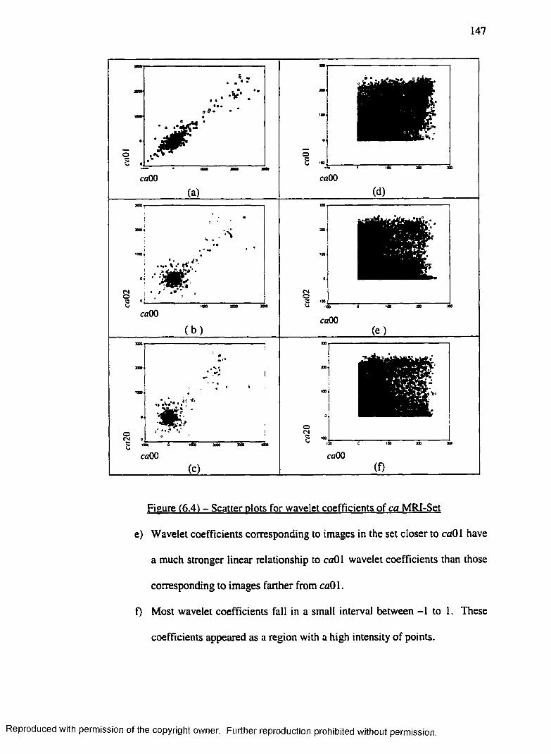
147
caOO
(a)
©
caOO
(d)
caOO
( b )
eso2
caOO(e)
ofN
caOO(C)
OCN5 too
caOO(f)
Figure (6.41 - Scatter plots for wavelet coefficients of ca MRI-Set
e) Wavelet coefficients corresponding to images in the set closer to caOl have
a much stronger linear relationship to caOl wavelet coefficients than those
corresponding to images farther from caOl.
f) Most wavelet coefficients fall in a small interval between -1 to 1. These
coefficients appeared as a region with a high intensity of points.
Reproduced with permission of the copyright owner. Further reproduction prohibited without permission.

148
xfo
ccOO(a)
ccOO
( d )
<N%
ccOO ccOO( b ) ( e )
"ToSo"
ccOO ccOO( c ) ( f )
Figure (6.5) - Scatter plots for wavelet coefficients of cc CT-Set
Using these scatter plots, it is clear that linear regression fails when applied to
the original pixel-based images to predict the removed or missing image(s). The result
of prediction of the images of the MRI and CT set from the first image of their
respective set is shown in Table (6-13) and Table (6-14) respectively.
Reproduced with permission of the copyright owner. Further reproduction prohibited without permission.

149
Table (6-13) - Prediction of ca MRI images from the first image of the set (caOO) using linear regression analysis of the wavelet coefficients
Img. A P r fo oP correlation R /?"caOl 9.619*10" 1.004 0.089 0.002 0.881 0.894 0.777ca02 -6.32*10" 1.058 0.087 0.002 0.894 0.894 0.800ca03 -4.17*10*" 0.863 0.075 0.002 0.884 0.884 0.781ca04 -8.4*10*" 0.906 0.080 0.002 0.881 0.880 0.771ca05 -1.49*10*^ 0.955 0.079 0.002 0.894 0.894 0.800ca06 7.423*10'" 1.116 0.081 0.002 0.915 0.915 0.837ca07 7.647*10" 1.026 0.068 0.002 0.927 0.927 0.860ca08 4.589*10*" 1.068 0.065 0.002 0.938 0.938 0.879ca09 1.510*10"* 1.006 0.061 0.001 0.937 0.937 0.879ca 10 2.893*10*" 1.134 0.068 0.002 0.940 0.940 0.884c a ll 8.379*10" 1.151 0.069 0.002 0.940 0.940 0.884ca 12 3.723*10*" 1.158 0.068 0.002 0.941 0.941 0.886cal3 4.868*10*" 1.120 0.071 0.002 0.934 0.934 0.872ca 14 -1.92*10" 1.064 0.074 0.002 0.922 0.922 0.849ca 15 -1.5*10" 1.056 0.083 0.002 0.902 0.902 0.813ca 16 1.071*10*" 0.970 0.086 0.002 0.880 0.880 0.775ca 17 -4.45*10*" 0.928 0.092 0.002 0.856 0.856 0.733c a l8 -2.52*10"* 0.702 0.079 0.002 0.827 0.827 0.683ca 19 -6.5*10'" 0.719 0.091 0.002 0.792 0.792 0.627
Reproduced with permission of the copyright owner. Further reproduction prohibited without permission.

150
Table (6-14) - Prediction of cc CT images from the first image of the set (ccOO) using linear regression analysis of the wavelet coefficients
Img P. P oPo oP correlation R Rf
ccOl -3.07*10'" 0.961 0.073 0.001 0.956 0.956 0.913cc02 -3.44* 10"1 0.968 0.085 0.001 0.942 0.942 0.888cc03 0.94*10" 0.930 0.081 0.001 0.943 0.943 0.889cc04 3.4* 10'2 0.985 0.096 0.002 0.929 0.929 0.864cc05 1.23*10" 0.887 0.082 0.001 0.936 0.936 0.877cc06 2.23*10" 1.031 0.096 0.002 0.935 0.935 0.874cc07 1.24*10'" 0.938 0.910 0.001 0.930 0.930 0.864cc08 3.23* 10° 0.909 0.085 0.001 0.935 0.935 0.873cc09 -3.88*10'" 0.969 0.085 0.001 0.941 0.886 0.941cclO 7.22*10'" 0.963 0.089 0.001 0.936 0.936 0.877ce ll 0.137 0.955 0.100 0.002 0.920 0.920 0.846ccl2 7.068*10° 0.912 0.086 0.001 0.934 0.934 0.872ccl3 9.075*10" 0.935 0.101 0.002 0.915 0.915 0.837ccl4 5.548*10'" 0.933 0.075 0.001 0.951 0.951 0.904cc!5 6.199*10'" 0.918 0.091 0.001 0.927 0.927 0.860ccl6 -5.64*10'" 0.909 0.075 0.001 0.949 0.949 0.900cc!7 9.371*10'" 0.985 0.080 0.001 0.950 0.950 0.902cc l8 5.525* 10'j 0.968 0.074 0.001 0.955 0.955 0.911ccl9 7.008*10° 0.846 0.078 0.001 0.937 0.937 0.877
The following conclusions for this chapter are limited to the wavelets used:
1. The wavelet coefficient series of a set of similar images is more correlated than the
images (pixel series) themselves. Thus, prediction of missing or removed images
can be done more accurately using the wavelet coefficients of a similar image set.
2. Using CDF(5,5) with the level 5 of decomposition was sufficient for prediction of
the brain images of the set used in this study.
3. The linear regression between images and wavelet coefficients showed that linear
regression can be used on the wavelet transform coefficients obtained by CDF(5,5)
to predict the missing or removed image(s) of a medical similar image set.
Reproduced with permission of the copyright owner. Further reproduction prohibited without permission.

151
In a similar image set, the average image generally produces better correlation
(prediction) quality both in the original (pixel) and transformed (wavelet) domain.
Reproduced with permission of the copyright owner. Further reproduction prohibited without permission.

CHAPTER 7
EXPERIMENTAL RESULT: SET COMPRESSION USING LIFTING ASSOCIATED WITH THE NEW SCANNING TECHNIQUES
7.1 Introduction
In Chapter (5), a result for the selection of a best wavelet basis was presented.
In Chapter (6) the result of prediction of some images of a similar set from an image in
the set was presented. In both chapters the analysis was done on the wavelet
coefficients representing the images of the image sets. These were the real values
used to reconstruct the original images. The reconstructed images were real and were
rounded to integers to obtain the original image. The rounding process can result in a
loss of data. In this chapter, a lifting scheme is used with scanning techniques to
address the problem of data loss. The first phase determines the lifting schemes that in
conjunction with the scanning methods generate the lowest entropy. Such a
combination should improve the compression of the medical image set.
7.2 Comparison of Lifting Schemes and Scanning Methods
The five image sets used in Chapter (5) are used to determine the best lifting
scheme. Figure (7.1) through Figure (7.5) present the results for different lifting
schemes in conjunction with scanning techniques. These figures were obtained by
computing the entropy of the coefficients for the wavelets after lifting the images of
the es, eb, et, si, and cc sets respectively. The images after lifting are represented as
integers. The lifting schemes and scanning methods used are shown in Table (7-1).
152
Reproduced with permission of the copyright owner. Further reproduction prohibited without permission.

153
Table (7-1) - List of lifting schemes and the scanning techniques
No. Wavelet Lifting/Scanning No. Wavelet Lifting/Scanning
WO Haar W21 (9,7) / vertical scanning
W1 CDF(2,2) W22 (9,7) / diagonal scanning
W2 CDF(2,2) / spiral scanning W23 CDF(2+2,2)(1)/ spiral scanning
W3 CDF(2,2) / horizontal scanning W24 CDF(2+2,2) (1)/ horizontal scanning
W4 CDF(2,2) / vertical scanning W25 CDF(2+2,2) (1)/ vertical scanning
W5 CDF(2,2) / diagonal scanning W26 CDF(2+2,2) (1)/ Diagonal scanning
W6 CDF(2,2) / rows then columns, xy W27 CDF(2+2,2) (2)/ spiral scanning
W7 CDF(4,2) / spiral scanning W28 CDF(2+2,2) (2)/ horizontal scanning
W8 CDF(4,2) / horizontal scanning W29 CDF(2+2,2) (2)/ vertical scanning
W9 CDF(4,2) / vertical scanning W30 CDF(2+2,2)(2)/ Diagonal scanning
W10 CDF(4,2) / diagonal scanning W31 CDF(2+2,2)(3)/ spiral scanning
W ll CDF(6,2) / spiral scanning W32 CDF(2+2,2)(3)/ horizontal scanning
W12 CDF(6,2) / horizontal scanning W33 CDF(2+2,2)(3)/ vertical scanning
W13 CDF(6,2) / vertical scanning W34 CDF(2+2,2)(3)/ Diagonal scanning
W14 CDF(6,2) / diagonal scanning W35 CDF(4,2) / rows then columns, xy
W15 D4 / spiral scanning W36 CDF(4,4) / spiral scanning
W16 D4 / horizontal scanning W37 CDF(4,4) / horizontal scanning
W17 D4 / vertical scanning W38 CDF(4,4) / vertical scanning
W18 D4 / diagonal scanning W39 CDF(4,4) / Diagonal scanning
W19 (9,7) / spiral W40 CDF(4,4) / rows then columns, xy
W20 (9,7) / horizontal scanning
Reproduced with permission of the copyright owner. Further reproduction prohibited without permission.
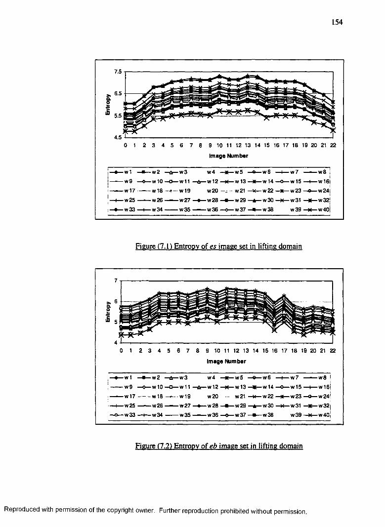
154
0 1 2 3 4 5 6 7 8 9 10 11 12 13 14 15 16 17 18 19 20 21 22
Im age Number
w 1 —■— w2 —&— w3 w4 —*— w5 - a -w 6 —1— w7 — ■— w8w9 —o— w 10 - o — W11 w12 — w13 —*— w 14 —o— w 15 —I— w16w17 — — w18 w19 w20 — - w21 —* - w 2 2 —* — w23 —o ■ w24
w25 -------w26 ------- w27 —♦— w28 w29 —6— w30 w31 K w32
w33 — I— w34 -------w35 — -w 36 —o— w37 —e— w38 w39 - K w40J
Figure (7.1) Entropy of es image set in lifting domain
— w l ■ w2 —a - w3 w4 —«6— w5 —e - w6 —I— w7 ■ - w8
1-------w9 —0— w10 -O — W11 —A—w12 - K — w13 MC w14 —o— w15 —(— w16
i - w17 -------w 18 — w19 w20 - w21 - M— w22 w23 - o — w24
i—♦— w25 -------w26 — w27 w28 ■ w29 —A— w30 - X - w31 —m— w32! - o — w33 —1— w34 -------w35 ------- w36 —0— w37 —• — w38 w39 —H— w40
Figure (7.2) Entropy of eb image set in lifting domain
Reproduced with permission of the copyright owner. Further reproduction prohibited without permission.
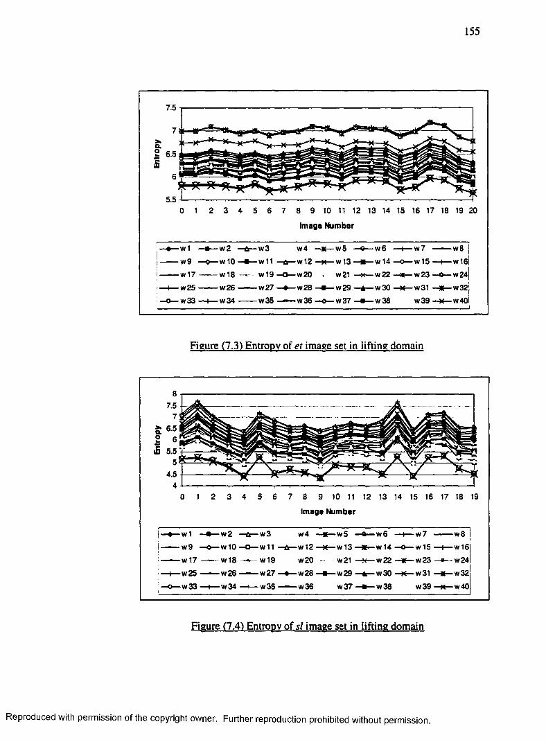
155
7.5
0 1 2 3 4 5 6 7 8 9 10 11 12 13 14 15 16 17 18 19 20
Image Number
1 w l —■— w 2 —tx— w3 w4 w5 —e — w6 —I— w7 — — w81____ w9 —0— w 10 w11 —A— w 12 - X — w13 —* — w 14 —o— w 15 —I— w16l
w17 — w18 w19 —o — w20 , w21 -K— w22 ■X— w23 —o— w24
w25 ------- w26 — — w27 » w28 —• — w29 —A— w30 —*t— w31 - M w32
— ° — w33 —I— w34 -------w35 -------w36 —O— w37 —e — w38 w39 - x — w40
Figure (7.31 Entropy of et image set in lifting domain
0 1 2 3 4 5 6 7 8 9 10 11 12 13 14 15 16 17 18 19
Image Number
| w 1 —e — w 2 w3 w4 —* — w5 —a— w6 —i— w 7 — w8 I! t— w9 —> — w 1 0 —O— w11 - A -w12 - K - w13 HK w 1 4 —o— w 1 5 —I— w16
i - w 1 7 ------ w 1 8 —— w19 w20 - w21 —x— w22 —* — w23 —•— w24i:— I— w25 — ■— w26 —— w27 ♦ w28 —• — w29 A w30 K- w31 * w32
—o— w 3 3 —(— w 3 4 —i— w35 — w36 w37 —■— w38 w39 K w40I_________
Figure (7.4) Entropy of si image set in lifting domain
Reproduced with permission of the copyright owner. Further reproduction prohibited without permission.

156
0 1 2 3 4 5 6 7 8 9 10 11 12 13 14 15 16 17 18 19 20
Im age Number
w 1 —■— w2 w3 w4 w5 -® — w6 —1— w7 — ■— w8w9 —O— W10 —a— w11 -A —w12 —X—w 13 —*—W14 - o — w15 —1— w16w17 ------w18 - - - w19 w20 —x - w21 k ■ w 22 — w23 - o — w24w25 -------w26 — —w27 - w28 w29 * w30 w31 IK ■ w32
w33 —1— w34 —*— w35 ------- w36 —O— w37 —■— w38 w39 K w40
Figure (7.5) Entropy of cc image set in lifting domain
The following observations can be made with respect to lifting and
scanning:
• The CDF(2,2), CDF(4,2), and CDF(4,4) applied to each row then column
in a 2-D image generated the lowest entropy for each set. The worst result
occurred for CDF(2+2,2) with option (3) coefficients in Equation 3.85.
• CDF(2,2) uses fewer coefficients than CDF(4,2) and CDF(4,4), and is a
better choice.
Two sets, CT-Set with 20 CT images of the spleen, and MRI-Set with 20 MRI
images of the brain were used for testing. All images are 256x256, grayscale, and
shown in Appendix B. Before the lifting, one background isolation technique (spiral.
Reproduced with permission of the copyright owner. Further reproduction prohibited without permission.

157
vertical, or horizontal) is selected to determine the background. The results for these
determinations are presented as an approximate percentage of the whole image that is
background on Figure (7.6) and Figure (7.7). For the CT-Set, the horizontal isolation
determined the highest percentage of background pixels (29.4% of the image set),
spiral (11.4%) and vertical isolation (6.4%). For the MRI-Set, vertical isolation had
the largest percentage of background pixels (33.5%), spiral isolation (28.8%) and
horizontal isolation (20.4%).
30000
25000
20000
15000 -
10000
5000
Image
□ SBIM(11.47%) ■ VBIM(6.4%) DHBIM(29.4%) ;
Figure (7.6) - Comparison of the background isolation techniques on the spleenCT-Set
On Figure (7.6) and Figure (7.7) the percentage of background varies
depending on the shape and the scanning of an image. For the CT-Set on Figure (7.6),
the lowest percentage background was determined for image “s/03” with spiral
isolation. The highest percentage background was determined for image “s/05” with
horizontal isolation. The results for the MRI-Set on Figure (7.7) show that, the lowest
Reproduced with permission of the copyright owner. Further reproduction prohibited without permission.

158
percentage of background is determined for image “e/03” with spiral isolation, and the
largest isolated background was obtained for image “e/20” with spiral isolation also.
M«X£■oe
oam
40000
35000
30000
25000
2000015000
te 10000 -2E3z
5000
0
t i t
— m in<5 9 9D U O
r»9u
— cou o
ino
r~o
e>o
Image
□ SBIM(28.8%) ■VBIM(33.5%) □HBIM(20.4%)
Figure (7.7) - Comparison of the background scanning techniques on the brainet MRI-Set
The variation in the percentage of background depends upon the scanning
technique. For example on Figure (7.8) the “continuous” background near the top of
image “e/03” has a protrusion in the diagnostic foreground near the top of the image.
The presence of this protrusion terminates the scanning of the “continuous”
background - because pixel intensities in that part exceed the threshold. This same
image with vertical isolation obtains a better background percentage for compression
purposes. Due to the existence of variations in the shapes of images, different
scanning methods are used to determine the approximate percentage of background.
On Figure (7.8), the diagnostic foreground of image “e/20” is a small part of the image
Reproduced with permission of the copyright owner. Further reproduction prohibited without permission.

159
and this results in effectiveness for spiral isolation. So, for each image depending on
the shape of the background and the diagnostic foreground, one scanning may work
better than the others.
One objective is to determine the amount of disk each image set requires
after being transformed by one type of lifting and compressed with a lossless
foreground compression. To obtain these results, we separated the “continuous”
background of the set from the set and applied lifting to the remaining foreground of
the set using 5 different lifting schemes. The wavelets used in the lifting were chosen
because of their popularity. The CDF(N, N ) wavelets are biorthogonal Cohen-
Daubechies-Feauveau wavelets with N and N representing the number of vanishing
moments for the high-pass synthesis and low-pass analysis filters respectively
[Calderbank 96]. D4 refers to the Daubechies wavelets with 4 vanishing moments.
The Bi(9,7) is a symmetric biorthogonal wavelet used in the FBI Fingerprint
et03 er20
Figure (7.8) - The et03 and et20 MRI Images
Reproduced with permission of the copyright owner. Further reproduction prohibited without permission.

160
compression that has 9 low-pass and 7 high-pass coefficients. We also used Huffman
coding, LZ77, and LZW, on the lifted coefficient sets. The compression ratio was
obtained by dividing the disk space required by the transformed images by that of the
original images. Comparison of different scanning methods and different compression
techniques are shown on Figures (7.9) and (7.10) for the CDF(2,2) wavelet. For the
MRI-Set the vertical scanning together with the LZW yielded the smallest
compression ratio. For the CT-Set the modified spiral scanning together with LZW
generated the best result.
0.9 0.8 0.7
5 0.6 I 0.5
0.4 0.3 0.2 0.1
21 3 4
Scanning Method
Original —■— Isolated image LZWHuffman LZ77
Figure (7.9) - Comparison of the disk space taken bv the spleen CT-Set scanned by: 1) spiral. 2) modified spiral. 3) horizontal, and 4) vertical scanning methods.
Reproduced with permission of the copyright owner. Further reproduction prohibited without permission.

Scanning Method
■ Original —■— Isolated Image ■ a LZWHuffman —* — LZ77
Figure (7.10) - Comparison of the disk space taken bv the brain MRI-Set scanned by: 1) spiral. 2) modified spiral. 3) horizontal, and 4*1 vertical scanning methods.
The minimum disk space required for the sets by different lifting schemes are
shown in Table (7-2) and Table (7-3). The smallest disk requirement for the CT-Set
was obtained with modified spiral scanning and CDF(4,4) or CDF(2,2) lifting on the
1-D array representing the foreground area, b, and LZW for compression. Table (7-2)
presents a compressed image set that is 5.56 times smaller than the original set. Table
(7-3) presents the least disk required for the MRI-Set. This was obtained with vertical
scanning with CDF(6,2) lifting on array b, and LZW. This compresses the set
approximately 4.35 times. It is noted that the best compression is achieved by the
best combination of scanning method, lifting procedure, and coding technique. This
Reproduced with permission of the copyright owner. Further reproduction prohibited without permission.

162
means that the scanning method that produced the best determination of the
background may not necessarily result in the best compression. For example: Figure
(7.9) and Figure (7.10) may be used to select a scanning technique for determining
background pixels, but that scanning technique does not necessarily generate the most
friendly signal for the lifting and/or coding technique.
Table(7-2) - Comparison of minimum disk space obtained by different lifting schemes for the spleen CT-Set (JPEG-LS = 2.99 ratio)
LiftingScheme Compression
ScanningMethod
CompressionMethod
CDF(2,2) 5.56 Modified Spiral LZWCDF(4,4) 5.56 Modified Spiral LZWCDF(6,2) 5.52 Modified Spiral LZWBi(9,7) 5.27 Modified Spiral LZWD4 4.82 Spiral LZW
Table(7-3) - Comparison of minimum disk space obtained by different lifting schemes for the brain MRI-Set (JPEG-LS = 1.48 ratio)
LiftingScheme Compression
ScanningMethod
CompressionMethod
CDF(2,2) 4.34 Vertical LZWCDF(4,4) 4.11 Vertical LZWCDF(6,2) 4.35 Vertical LZWBi(9,7) 4.31 Vertical LZWD4 4.13 Vertical LZW
The decomposition was done on an SGI Origin 2000 using C. The elapsed
time for isolation and lifting of the CT-Set and MRI-Set were 5.35 secs and 9.8 secs
respectively. JPEG-LS [Winberger 99] required 0.7 secs for the CT-Set and 1.2 secs
Reproduced with permission of the copyright owner. Further reproduction prohibited without permission.

163
for the MRI-Set. The JPEG-LS time was obtained by adding the individual
compression time for each image of the set.
The scanning techniques in this dissertation significantly reduce the number of
edges. Lifting was used on sets of similar images with different diagnostic
foregrounds. The lifting scheme applied to the 1-D signal used on the CT-Set resulted
in a maximum compression of 5.56 with CDF(4,4) lifting with both the spiral
scanning and modified spiral scanning techniques. For the MRI-Set, the minimum
disk space was achieved with CDF(2,2) lifting and vertical scanning. JPEG-LS
[Winberger 99] compression of the CT-Set was 2.99 and for the MRI-Set 1.48. The
conclusion is the scanning method plus an appropriate lifting scheme can be used to
improve the diagnostically “lossless” compression of a set of medical images.
Reproduced with permission of the copyright owner. Further reproduction prohibited without permission.

CHAPTER 8
THE OPTIMAL WAVELET BASIS: AN OVERVIEW OF A THEORETICAL APPROACH
8.1 Introduction
The optimal wavelet basis selection presented in Chapter 5 was based upon
experimental approach to determine an optimal basis from a selection of known
wavelets for particular sets of medical images. In reality, the optimal basis found for
one set of medical image may not necessarily be optimal for other medical images. In
addition, there are practically an infinite number of wavelets from which to choose.
The question then would be, how to determine the optimal basis for all medical
images. If we could construct a set of medical images of an organ that covers almost
every reasonable-possible radiological study of that organ. Then we could argue thati
since the result was optimal for the set of almost every reasonable-possible
radiological study, it could be assumed to be optimal by rational argument. The
difficulty with this procedure is that constructing an image set that consists of almost
every reasonable-possible radiological study is very difficult to do and probably
impractical. Another approach would be to find or develop a theoretical method that
applies to the medical image sets of interest and determine their optimal wavelet basis.
In recent years, there has been a substantial amount of research to find optimal
wavelet bases. One task to finding an optimal wavelet basis is determining an
appropriate parameterization and an adequate performance measure. In addition, the
accurate interpretation of physical phenomena has a major role [Zhuang 94a][Zhuang
94b]. A method introduced by [Tewfik 92] and [Jorgensen 93] is based upon
164
Reproduced with permission of the copyright owner. Further reproduction prohibited without permission.

165
minimization of an upper bound of the L2 norm of the error in approximating a signal,
up to the desired scale. An entropy based algorithm for determining an optimal
wavelet basis has been presented [Coifman 92] where the optimal basis is selected
from a library of wavelets. In more recent work, [Zhuang 94a][Zhuang 94b], the
optimal orthonormal discrete wavelet basis with compact support was generated
directly. This algorithm constructs the optimal wavelet basis based on the signal. In
this chapter, the method of constructing an orthogonal wavelet basis is presented, then
the optimal orthogonal wavelet basis will be theoretically determined and
demonstrated on medical images used in this research. In general, the goal is to
determine an optimal basis for medical images.
8.2 Construction of Compactly Supported Orthogonal Wavelets
Most of the material in this section is based on and taken from the theory in
Chapter 7 of [Chui 92]. Suppose there exist two sequences {p*/ and {qij 6 Lr such
that;
<t>(x) = ' £ p k0 { 2 x -k ) 8.1k
and,
i/f(x) = ' £ q l 0 ( 2 x - k ) , 8.2k
for all .re/?. These two formulas are called "two-scale relations" of scaling and
wavelet functions respectively. There is a relationship between the scaling function
and wavelet;
i y ( x ) £<7*^2 x - k ) 8.3k e Z
where.
Reproduced with permission of the copyright owner. Further reproduction prohibited without permission.

166
8.4
Also, we can write the following;
yfJ t (x) = 2 j,z iy(2Jx - k ) , j , k e Z 8.5
This means that we can construct an orthogonal wavelet y / , by constructing its
corresponding orthogonal scaling function <f>. For simplicity, we only consider real
valued two-scale sequences {prf. The need is to identify a Laurent polynomial S(z),
corresponding to any given positive integer N, such that the following conditions are
satisfied:
Where P , the two-scale symbol of some scaling function <f>, is a Laurent series in
Wiener Class, i.e. the two-scale sequence belongs to I1. We are interested in those P
that can be expressed as:
where N is some positive integer, and S s W satisfies S(l) = 1.
All Laurent series satisfy < 00 for some e > 0. That means that we
only need to Find those S’s that satisfy 8.7 and the bounds:
P(l) = /, and
IP^I2 +\P(-z)\2 =1, |z|=/•
8.6
8.7
8.8
5 := max|SU)| < 2 * '1. 8.9
Then for any S in 8.8, we can write:
S{z) = Y , s kz k;i 8.10
B max | S(z) |. 1=1=1
Reproduced with permission of the copyright owner. Further reproduction prohibited without permission.

167
The goal is to find a useful condition to factor S such that P is guaranteed to be a two-
scale symbol of some orthogonal scaling function, <p. Then, the infinite product:
g w - n p r ' - )*=l
8.11
will converge to g e C(R) n Ll(R )n L r(R ) everywhere, and <j> e LZ(R) , with 0 = g is
an orthogonal scaling function that generates a multi-resolution analysis (MRA) of
LZ(R).
To translate 8.7 into a relation that involves S(z), we take advantage of the fact
that S is a Laurent polynomial with real coefficients, | S(e~'“ ) |2= R (cos co), where R
is some algebraic polynomial with real coefficients. Using the following change of
variables:
1-co sty . •,.(!).■r = ---- = stn*(—);
R(x) = R(cosco) = R( 1 - 2jc),8.12
we will obtain for 8.7:
l + e" l-e~2N
1 |: = I, 8.13
which can also be written is terms of x:
( l - x ) A'K(;c) + .t*K(l-x) = l. 8.14
The general solution to this equation is:
(x) = £l k r +x ^ 8.15
where T is a polynomial with T(l-x) = - T(x). For any Laurent polynomial that
satisfies both 8.10 and:
Reproduced with permission of the copyright owner. Further reproduction prohibited without permission.

f t - 2*^then for some odd polynomial T0 (*) := 71— , the Laurent polynomial can be
wntten:
l+ z = 817
in which 5(1) is chosen to be 1. 5(1) is the two-scale symbol of some compactly
supported orthogonal scaling function $ that generates an MRA for L:(R). This
results in:
ir ( x ) ~ ' £ { - l ) kp_k, l<t>(2x-lc), 8.18k
which is a compactly supported orthogonal wavelet. If 5 satisfies 8.16, then
|S(l)|: = I for co = 0 , thus the condition 5(1) = I is achieved. The family of all odd
polynomials Ro(x), i.e., |.r| < -^, in 8.16 provides some freedom in constructing an
orthogonal $ . If by choosing Ro ~ 0, we do not violate 8.8, then the corresponding <p
will have the smallest support among all the Laurent polynomials obtained by 8.16.
The condition in 8.10 is satisfied by the choice of Ro = 0.
Suppose, 5(z) is a Laurent polynomial with real coefficients that satisfies:
£ 1 1 J 2for any positive integer N such that S(l)=l. Then, S(z) is the two-scale symbol of a
compactly supported orthogonal scaling function 0 and wavelet i ff. Therefore, to
Reproduced with permission of the copyright owner. Further reproduction prohibited without permission.

169
construct a compactly supported orthogonal wavelet, we solve 8.19 for S(z). The
following theorem proves that such a solution exists.
Theorem 8.1. Suppose we have a sequence aQ,ax,---,aN e R with aN * 0 such that:
8.20A (ty).- — + coska) > 0, a>eR.~ *=» i
Then there will be a polynomial:
= 8-21*=»o
with real coefficients and degree N that satisfies:
| B{z) |2= A{(0 ), z = e-"°. 8.22
Proof: Let’s consider the algebraic polynomial:
8-23- k=-N
which corresponds to the cosine polynomial A(af). In 8.23, Pa will satisfy:
PA(z) = z “A(at), z = and 8.24
nPa ( z ) = V n Pa \ -
\ z jz e C . 8.25
By assuming aN * 0 , we will have PA * 0, then, in 8.25, all the zeros of Pa occur in
reciprocal pairs. Moreover, any zero on the unit circle is required to have even
multiplicity. Then, since coefficients PA are real and the complex zeros of Pa also
occur in conjugate pairs, PA can be written as:
? a (z) = | 'aN j l l 1 ~ rt ~ rt l ) |:* j n 1 ~ z i )(z ~ l i Xz ~ z 7 K z ~ z 7‘ > j’ 8-26
where rl ,rz, --,rK € R \ {0},z, , e C \ R , and AT+27=M Thus, using:
Reproduced with permission of the copyright owner. Further reproduction prohibited without permission.

170
| ( Z - Z j )(z- zjl) H Z; r u - Zj r . z = , 8.27
and by applying 8.22,8.24,8.26, and 8.27, we will obtain:
i n i '- ." i n u , r *t=t 7=1
K Jn^-onb-^xz-z,)*=l 7=1
8.28
where z = e'“° . Thus, the polynomial:
B(z) =
I
\\as i n i r*_ti n i r2 4n(z^)n(z-z,)(z-z;)l 8.291 »=< .=t j i * = i 7=1 j*=1 7=1
will satisfy 8.22 and has degree N=K+2J.
This equation can be used in conjunction with 8.19 to obtain the scaling
function.
8 J Optimal Discrete Wavelet Basis
Several methods for finding the optimal wavelet basis are presented in
[Coifman 92][Ramchandran 96][Chen 95][Zhuang 94a], and [Zhuang 94b].
The method presented in [Coifman 92] relies on building a library of wavelet
functions of orthogonal bases relative to which a given signal or collection of signals
has the lowest information cost. The method basically targets bases with O(NlogN)
transformation algorithms with natural dyadic tree structure that provides O(NlogN)
search algorithms for finding the optimal basis. The libraries are constructed without
storing the analysis or synthesis parts. This method relies on the orthogonality
properties of the new libraries. Since the selected orthogonal transformation that
Reproduced with permission of the copyright owner. Further reproduction prohibited without permission.

171
represents the signal is a nonlinear function of its own optimal basis, the compression
via the optimal basis is not significantly affected by noise.
The method presented in [Ramchandran 96] achieves the lowest overall cost by
making the transformation vary with the signal type. Since there are an infinite
number of options, minimizing the cost for all possible transforms is not feasible.
Thus, a very large (but finite) library of useful transforms is selected. Then, to make
the method more effective, the library is organized in such a way that the search for
the optimal base is easier.
The method presented by [Chen 94] is a new criteria, "wavelet transform
coding gain" that is based on the relationship between scalar quantization error and
vector quantization error of the applied coding scheme. The method optimizes the
quantizer with different bit allocation. This technique investigates the cross
correlation among subbands to improve the coding efficiency by efficiently employing
the dependencies among subbands. The method exploits these dependencies among
subbands by examining the maximum directional variation in each small block of
base-band images and the maximum wavelet amplitude in the corresponding block of
upper band images.
Although the above techniques had some success in determining an "optimal"
wavelet basis, none generated the optimal wavelet basis. There are two algorithms
proposed [Zhuang 94a], [Zhuang 94b] to obtain an optimal wavelet basis. They are
inspired by the work done by Coifman et. al. This proposed process for finding an
optimal wavelet basis is to first find a parameter set {c*} such that an additive
information measure, in this research it’s entropy, is minimized. Once the set {c*}is
Reproduced with permission of the copyright owner. Further reproduction prohibited without permission.

172
determined, the scaling function <f> and wavelet base ^can be derived. Before
presenting these two algorithms, we define additive information measure.
Definition 8.1: An additive information measure is defined as a non-negative map M
from a sequence [/!} to R if M(0) = 0 and M (^ \ f t).
Definition 8.2: For a fixed vector x e R N and the collection of all orthogonal bases of
dimension N, B, a basis Be Bis optimal if M(Bx) is minimal for all bases in B with
respect to the vector x. The Shannon entropy is defined:
XX
This represents a measure of the information content of a random variable X.
Definition 8.3: In a Hilbert space defined as an orthogonal direct sum:
in 8.32 and it is the equivalent probability measure in the decomposition entropy. The
maximum entropy corresponds to a signal with uniform energy distribution in its
frequency domain. On the other hand, a lower entropy value means a higher
8.30
8.31
the decomposition entropy is defined as:
8.32
for v€ //,||v|| * 0 , such that:
v © £ v , , v,e H,, 8.33
and (p)log(p)=0, where p=0.
In 8.32, the is the stochastic approximation of Shannon entropy defined
Reproduced with permission of the copyright owner. Further reproduction prohibited without permission.

173
concentration of the signal energy over certain frequencies. To find an optimal
wavelet basis for a set of images, one needs to find a wavelet for that class of image
which results in a higher energy concentration over a certain frequency band.
In Chapter (1), we showed that any square integrable function
f ( x ) E L(RZ) can be represented as:
f (x) = '£tWjjV'Jj W - 8-34jj
By choosing M and N as the appropriate positive integers, we can write 8.34 as:
/(*)= Z 8-35l = - N
over a mesh size of (2M+1)(2N+1). The goal is to find the optimal wavelet basis
function y/{t) for a given signal fix) such that the additive information is minimal.
There is still one problem to be resolved; the decomposition entropy is a good measure
of ’’distance", but is not an additive type of map because the norm||v|| is used to scale
the vector. Thus, we introduce a new function:
A(<F,v) = - £ | |v j - lo g |v J’ . 8.36j
This relates to the decomposition entropy:
*(v,¥0 =||v|r2A(0,v) + log||v||2(2M +1). 8.37
This is an additive measure. Since both 8.36 and 8.37 share the same set of minimal
points, we minimize A(#,v) to find the optimal wavelet basis.
The sensitivity gradient - ■ ■ of the component iff ,d of the wavelet basisoc*
with respect to the parameter c* is given by:
Reproduced with permission of the copyright owner. Further reproduction prohibited without permission.

174
See Lemma 3.1 [Zhuang 94b] for the proof.
Since, we use A from 8.36 and 8.37 as the additive information measure, we
compute the sensitivity of the additive measure with respect to c*:
where [0,K] is the compact support for {c*} and V7 corresponds to the wavelet basis
formed by dilations and shifts of the wavelet if/it) . In equation 8.39, f(t) is a fixed
signal in L2(R), see Theorem 3.1 [Zhuang 94b] for the proof.
8.4 Algorithms for Finding an Optimal Wavelet Basis
The goal is to find a set of parameters {c*} such that the additive information
measure A is minimized. Once the set {c*} is determined, we can derive both the
scaling function 0 and the wavelet function if/ . The following is the first algorithm
presented in [Zhuang 94a] and [Zhuang 94b].
Algorithm 8.1: Determining the optimal wavelet basis as presented in [Zhuang 94a]
Step 0: Set i = I,4> = 0,
Step 2:
Step 3:
mesh parameters M, N;Initialize vector co;Input f[t)If d does not satisfy the constraint, then modify Cj and repeat Step 2.
a = c,./ + — .
Step 4 Step 5 Step 6
Compute 0 and iff. Compute A .lf\At - A,., | > e , i — i + 1 ,
Reproduced with permission of the copyright owner. Further reproduction prohibited without permission.

175
goto Step 2.Step 7: Output the optimal basis iff and stop.
The parameters M and N can be predetermined by the time and frequency localization
property of the desired signal. We can also use an adaptation scheme to appropriately
generate the system. The following is an algorithm for a variable mesh size.
Algorithm 8.2: Determining the optimal wavelet basis with variable mesh size from
[Zhuang 94a]:
Step 0: Set i - 1,^ o = 0,mesh parameters M, N;
Initialize vector co;Input fit).
Step 2: If Ci does not satisfy the constraint, then modify Ci and repeat Step 2.e , WStep 3: ci - a .j + p,_, - — •oc,_.Step 4: Compute and if/.Step 5: Compute X .Step 6: If \Xt - \ > £,
i = i +7 ,M = M +l,N = N+I ,
goto Step 2.Step 7: Output the optimal basis yr and stop.
This algorithm starts from an initial mesh size and adjusts the mesh size until
the error tolerance is met, while it updates the values of {c, }.
8.5 Results
To obtain the optimal wavelet basis, a computer program was written:
• to construct compactly supported orthogonal wavelets for a given medical
image set, then
• to determine the optimal wavelets for that set.
Reproduced with permission of the copyright owner. Further reproduction prohibited without permission.

176
Stepl: Construction of the compactly supported orthogonal wavelets
The compactly supported orthogonal wavelets were constructed using the
procedure presented in section 8.2. A summary of programmed calculations follows:
■> 1 — cos(ty)• 8.16 was written in terms of the cos(gj) using [sin (^ )]‘ = ----- .
• Then, Theorem 8.1 was used to find:
anA, = + a, cos(ty) + ••• + <*, cos'" (<y).
• A, is used to construct Ay
A, = a m+ an_i cos (a)) + am_2 cos z{qj) + ■■■
+ -cosm{(o) + a l cosm+l (cti)+ -- + am cosZm(a)).
• Then, the roots of A2W, a polynomial in jc = cos(ty), are determined.
• 8.29 is formed using only the roots from A: that satisfy jc;| > 1.
• The Laurent polynomial S(z) - C * B(z) is computed, where C is defined
with S(l) = /, initially.
• Finally, 8.8 obtains the new wavelet coefficients, wn, with "wavelet order"
n = l,2 ,-,10 .
Step 2: Determination of the Optimal Wavelet Basis
• The images are read and stored in an array.
• This array is transformed using one of the wavelets, wn, generated in Step
1 to create the wavelet coefficients.
• The resulting coefficients are compressed using thresholding.
Reproduced with permission of the copyright owner. Further reproduction prohibited without permission.

I l l
• The optimal wavelet basis is determined by calculating the lowest mean-
square fit corresponding to a selected range of wavelet parameter vectors T,
i.e., from [r0,* , , • • • , This vector can be of any dimension, i.e.,
T = [1,2,-**, ATI, or empty T= [ ] which is equivalent to T = [0,0,- -,0].
• The percent recovery is generated to determine how accurately the selected
wavelet reconstructs the image set.
For illustration, three examples of the many plots that have been generated in
Step 2 are presented on Figures (8-1), (8-2), and (8-3). Figure (8-1) presents the
percent recovery of the et MRI-set with w2 when 2 levels of decomposition are used.
Figure (8-2) and (8-3) present similar results for the db set with vv2-level 2 and cc
combined with the si set with w4-level 4, respectively.
W».9r-------------- 1-------------- 1----------------------------- 1------- \
99 8 - -
99 . 7- J
9 9 6 - '■
99 5 - / : -
99 4 - ■ '
i
99.3 \\ ' ,
!99 2 - -
9 9 1 - \
9 9 r1
QA * . . . i . . l ... •-------- J 1QA Q i i •
1 2 3 4 5 6 7 8 9 10
t
Figure (8-1) - Percent recovery of the et MRI-set using wavelet w2 which has 2levels of decomposition.
Reproduced with permission of the copyright owner. Further reproduction prohibited without permission.

178
100 p
t
99.8 rIj
9 9 6 rII
%99 4 h
99 2 r
98.8
986
■./•1
\ / v
1 2 3 4 5 6 7 8 9 10
Figure (8-2) - Percent recovery of the db MRI-set using wavelet w4 which has 4 levels of decomposition.
100-
99.951-
T ""I1\ I i
f
%
99.9-
99.85 r
99.81-
i99.75)-
99.7-4 -3 -2 -1
Figure (8-3) - Percent recovery of the si and cc CT-set combination, using wavelet w4 which has 4 levels of decomposition.
Reproduced with permission of the copyright owner. Further reproduction prohibited without permission.

179
On Figure (8-2), the w4 orthogonal wavelet with 4 levels of decomposition
produces perfect reconstruction at t = 7, 9, and 10. The optimal wavelet coefficients
are obtained at t = 10. None of the t values shown on Figures (8-1) and (8-3) resulted
in perfect reconstruction. The optimal wavelet coefficients are obtained at t = 2 for
both these cases.
Additional results obtained from these calculations are presented in Tables (8-1
through 8-11) and Figures (8-1 through 8-9).
Table (8-1) presents the wavelet coefficients of the optimal wavelet basis,
wl, vv2, vv3, • • •, w9, obtained at the decomposition level 2 for the db MRI-set. For
illustration, the optimal basis, wl,w2, w3,---,w9, obtained at a decomposition level 2
using the db MRI-set, are shown on Figures (8-4) through (8-8).
1 r0.80.6
cft 0.4Osr 0.28 0 -o -0.2 -
-0.4 --0.6 -L
8o
2
1
0
1
-2N
Figure (8-4) - Coefficients of the optimal wavelet basis: (Left) w l at decomposition level 2 and (Right) w2 at decomposition level 2.
Reproduced with permission of the copyright owner. Further reproduction prohibited without permission.
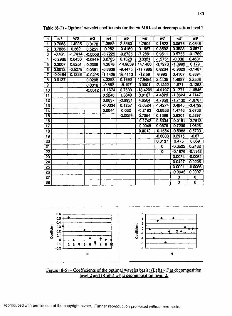
180
Table (8-1) - Optimal wavelet coefficients for the db MRI-set at decomposition level 2
n w 1 W 2 w 3 w 4 w5 w 6 w 7 w 8 w 9
1 0.7088 1.4925 0.3178 1.3682 2.5383 1.7604 0.1823 0.0678 0.03482 0.7836 0.362 0.5251 -0.282 -0.4159 0.1667 0.8592 0.3523 -0.05713 -0.461 -1.7414 -0.0008 -3.7229 -9.2725 -7.2861 0.9511 0.5755 -0.17694 -0.2985 0.6458 -0.0919 3.2763 6.1628 3.3321 -1.5751 -0.036 0.46315 0.3007 0.6251 0.2309 4.3678 -14.9659 14.1486 -3.7273 -1.0992 0.1796 0.0012 -0.5078 0.0381 -5.6639 -9.4475 -11.7885 0.8204 -0.9622 -0.14877 -0.0484 0.1238 -0.0496 -1.1426 16.4113 -12.59 6.992 0.4107 0.83948 0.0137 0.0298 4.3288 0.1692 17.9454 2.4435 1.4987 2.25089 0.0018 -0.862 -8.197 3.0001 -7.1222 1.571 -3.126310 -0.0012 -1.1674 2.7633 -13.4209 -4.9197 0.1771 -1.054511 0.5248 1.3849 3.8187 4.4823 -1.8624 4.714712 0.0037 -0.9931 4.6564 4.7858 -1.7132 -1.876713 -0.0334 0.1257 -3.0524 -1.4274 0.4845 -3.479914 0.0044 0.032 -0.2183 -2.5858 1.4746 3.670615 -0.0059 0.7054 0.1396 0.8301 0.589716 -0.1742 0.8334 -0.0181 -2.761817 -0.0048 0.0379 -0.7209 1.062818 0.0012 -0.1554 •0.5988 0.879319 -0.0083 0.2915 -0.8720 0.0137 0.475 0.05921 0 -0.0522 0.246222 0 -0.1876 -0.114823 0.0034 -0.006424 0.0427 0.020625 0.0001 -0.006626 -0.0045 0.000727 0 028 0 0
C©0
1
0.60.50.40.30.20.1
0- 0.1- 0.2
8 9—1
64
I 01 -2 O .4
-6-8
i -H— t3-
Fiaure (8-5) - Coefficients of the optimal wavelet basis: (Left! w3 at decomposition level 2 and (Right) w4 at decomposition level 2.
Reproduced with permission of the copyright owner. Further reproduction prohibited without permission.

181
-10-15-20
O
2015105O'
-5-10-15
*-1 1 ! 1 1 ■
-3— 5— 7 ■ 9— 14- 15-17-
Fieure (8-6) - Coefficients of the optimal wavelet basis: (Left) w5 at decomposition level 2 and (Right) w6 at decomposition level 2.
r
♦♦
-10N
3 5 .7 9 1113151^1921232527
Figure (8-7) - Coefficients of the optimal wavelet basis: (Left) vv7 at decomposition level 2 and (Right) wg at decomposition level 2.
6
4cSi 2 Si
-2
-4
8 0(% S . - ' r -<*.° ' 3 5 7 9*l1J31517ft21 232527
Figure (8-8) - Coefficients of the optimal wavelet basis of w9 at decomposition level7
Reproduced with permission of the copyright owner. Further reproduction prohibited without permission.

182
The image shown on Figure (8-9) presents the w2 decomposition of et 10 at
level 2 and Figure (8-10) presents the reconstructed image. These demonstrate the use
of one of the optimal wavelet basis.
Figure (8-9) - The w2 level 2 decomposition of erlO
Figure (8-101 - The reconstructed erlO
Reproduced with permission of the copyright owner. Further reproduction prohibited without permission.
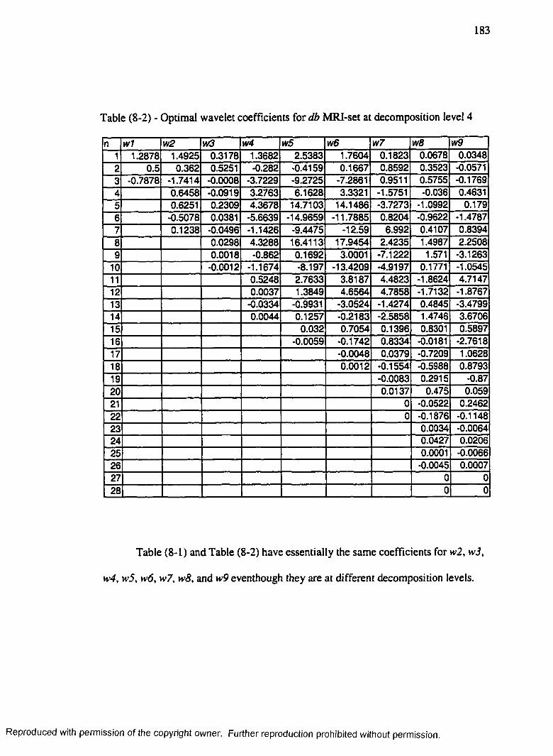
183
Table (8-2) - Optimal wavelet coefficients for db MRI-set at decomposition level 4
n w 1 w 2 w 3 W 4 w 5 w 6 w 7 w 8 w 9
1 1.2878 1.4925 0.3178 1.3682 2.5383 1.7604 0.1823 0.0678 0.03482 0.5 0.362 0.5251 -0.282 -0.4159 0.1667 0.8592 0.3523 -0.05713 -0.7878 -1.7414 -0.0008 -3.7229 -9.2725 -7.2861 0.9511 0.5755 -0.17694 0.6458 -0.0919 3.2763 6.1628 3.3321 -1.5751 -0.036 0.46315 0.6251 0.2309 4.3678 14.7103 14.1486 -3.7273 -1.0992 0.1796 -0.5078 0.0381 -5.6639 -14.9659 -11.7885 0.8204 -0.9622 -1.47877 0.1238 -0.0496 -1.1426 -9.4475 -12.59 6.992 0.4107 0.83948 0.0298 4.3288 16.4113 17.9454 2.4235 1.4987 2.25089 0.0018 •0.862 0.1692 3.0001 -7.1222 1.571 -3.1263
10 -0.0012 -1.1674 -8.197 -13.4209 -4.9197 0.1771 -1.054511 0.5248 2.7633 3.8187 4.4823 -1.8624 4.714712 0.0037 1.3849 4.6564 4.7858 -1.7132 -1.876713 -0.0334 -0.9931 -3.0524 -1.4274 0.4845 -3.479914 0.0044 0.1257 -0.2183 -2.5858 1.4746 3.670615 0.032 0.7054 0.1396 0.8301 0.589716 -0.0059 -0.1742 0.8334 -0.0181 -2.761817 -0.0048 0.0379 -0.7209 1.062818 0.0012 -0.1554 -0.5988 0.879319 -0.0083 0.2915 -0.8720 0.0137 0.475 0.05921 0 -0.0522 0.246222 0 -0.1876 -0.114823 0.0034 -0.006424 0.0427 0.020625 0.0001 -0.006626 -0.0045 0.000727 0 028 0 0
Table (8-1) and Table (8-2) have essentially the same coefficients for w2, w3,
w4, w5, w6, w7, w8, and w9 eventhough they are at different decomposition levels.
Reproduced with permission of the copyright owner. Further reproduction prohibited without permission.

184
Table (8-3) and (8-4) present the wavelet coefficients of the optimal wavelet
basis, >vl, w2, w3, • • •, w9, obtained at the decomposition levels 2 and 4 for the e t MRI-
set. Again the wavelet coefficients are essentially the same; however they are very
different from the wavelet coefficients shown on Tables 1 and 2.
Table (8-3) - Optimal wavelet coefficients for e t MRI-set at decomposition level 2
n w 1 w 2 w 3 W 4 w 5 w 6 w 7 w 8 w 9
1 1.1924 0.7489 0.3125 0.5993 2.5972 1.7676 1.4849 0.8833 0.02062 0.5 0.8409 0.511 0.2642 -0.4659 0.1648 -0.043 2.0195 0.01693 -0.6924 -0.6008 -0.0096 -1.492 -9.4716 -7.315 -5.4711 -3.9547 -0.1354 -0.3941 -0.0795 0.4387 6.4256 3.3512 4.8441 -9.8828 -0.06815 0.4592 0.249 2.2735 14.9097 14.1934 7.563 12.4882 0.43386 0.0199 0.037 -0.993 -15.4315 -11.8343 -15.7601 27.3662 0.08587 -0.1073 -0.0554 -1.2912 -9.3852 -12.612 2.835 -29.5229 -0.85178 0.0334 0.0336 1.0556 16.7282 17.9855 20.6442 -50.6607 0.06579 0.0034 0.4198 -0.0588 2.9863 -20.0122 54.9431 1.089210 -0.0025 -0.2716 -8.1971 -13.419 -7.1428 68.3152 -0.354211 -0.0093 2.8693 3.8318 23.683 -79.1803 -0.906612 0.0062 1.2942 4.6308 -10.2808 -67.8184 0.521913 -0.9773 -3.0457 -10.3634 88.9205 0.458314 0.1496 -0.2044 12.9414 49.3177 -0.418915 0.0166 0.6956 -1.0387 -76.9477 -0.103516 -0.003 -0.1752 -5.3688 -24.6772 0.195117 -0.002 2.415 50.6912 -0.018118 0.0005 0.5547 7.0181 -0.047819 -0.5957 -24.5337 0.016320 0.1111 0.2577 0.003721 0.0002 8.2808 -0.002822 0 -1.1235 0.000423 -1.7399 024 0.4268 025 0.172226 -0.058727 -0.000128 0
Reproduced with permission of the copyright owner. Further reproduction prohibited without permission.

185
Table (8-4) - Optimal wavelet coefficients for et MRI-set at decomposition level 4
n W1 w2 w3 w4 w5 w6 w7 w8 w91 1.1924 0.7489 0.3125 0.5993 2.5972 1.7676 1.4849 0.8833 0.02062 0.5 0.8409 0.511 0.2642 -0.4659 0.1648 -0.043 2.0195 0.01693 -0.6924 -0.6008 -0.0096 -1.492 -9.4716 -7.315 -5.4711 -3.9547 -0.1354 -0.3941 -0.0795 0.4387 6.4256 3.3512 4.8441 -9.8828 -0.06815 0.4592 0.249 2.2735 14.9097 14.1934 7.563 12.4882 0.43386 0.0199 0.037 -0.993 -15.4315 -11.8343 -15.7601 27.3662 0.08587 -0.1073 -0.0554 -1.2912 -9.3852 -12.612 2.835 -29.5229 -0.85178 0.0334 0.0336 1.0556 16.7282 17.9855 20.6442 -50.6607 0.06579 0.0034 0.4198 -0.0588 2.9863 -20.0122 54.9431 1.089210 -0.0025 -0.2716 -8.1971 -13.419 -7.1428 68.3152 -0.354211 -0.0093 2.8693 3.8318 23.683 -79.1803 -0.906612 0.0062 1.2942 4.6308 -10.2808 -67.8184 0.521913 -0.9773 -3.0457 -10.3634 88.9205 0.458314 0.1496 -0.2044 12.9414 49.3177 -0.418915 0.0166 0.6956 -1.0387 -76.9477 -0.103516 -0.003 -0.1752 -5.3688 -24.6772 0.195117 -0.002 2.415 50.6912 -0.018118 0.0005 0.5547 7.0181 -0.047819 -0.5957 -24.5337 0.016320 0.1111 0.2577 0.003721 0.0002 8.2808 -0.002822 0 -1.1235 0.000423 -1.7399 024 0.4268 025 0.172226 -0.058727 -0.000128 0
The coefficients for the et set are different from those for the db image set.
Thus, two different medical image sets do not have the same optimal wavelet basis.
Reproduced with permission of the copyright owner. Further reproduction prohibited without permission.
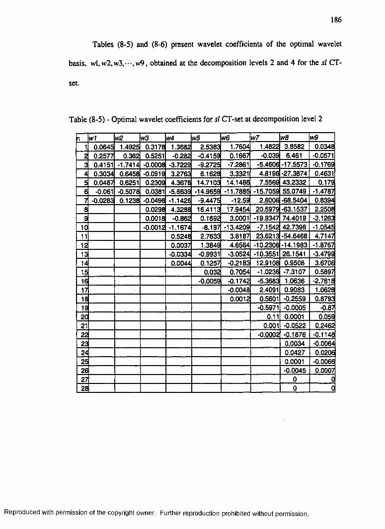
Tables (8-5) and (8-6) present wavelet coefficients of the optimal wavelet
basis, wl,w2,w3,---,w9, obtained at the decomposition levels 2 and 4 for the si CT-
set.
Table (8-5) - Optimal wavelet coefficients for si CT-set at decomposition level 2
n W1 w2 w3 W4 w5 w6 w7 w8 w91 0.0645 1.4925 0.3178 1.3682 2.5383 1.7604 1.4822 3.8582 0.03482 0.2577 0.362 0.5251 -0.282 -0.4159 0.1667 -0.039 6.461 -0.05713 0.4151 -1.7414 •0.0008 -3.7229 -9.2725 -7.2861 -5.4606 -17.5573 -0.17694 0.3034 0.6458 -0.0919 3.2763 6.1628 3.3321 4.8196 -27.3874 0.46315 0.0487 0.6251 0.2309 4.3678 14.7103 14.1486 7.5569 43.2332 0.1796 -0.061 -0.5078 0.0381 •5.6639 -14.9659 -11.7885 -15.7059 55.0749 -1.47877 -0.0283 0.1238 -0.0496 -1.1426 -9.4475 -12.59 2.8006 -68.5404 0.83948 0.0298 4.3288 16.4113 17.9454 20.5979 -63.1537 2.25089 0.0018 •0.862 0.1692 3.0001 -19.9347 74.4019 -3.1263
10 -0.0012 -1.1674 -8.197 -13.4209 -7.1542 42.7398 -1.054511 0.5248 2.7633 3.8187 23.6213 -54.6468 4.714712 0.0037 1.3849 4.6564 -10.2308 -14.1983 -1.876713 -0.0334 -0.9931 -3.0524 -10.3551 26.1541 -3.479914 0.0044 0.1257 -0.2183 12.9108 0.9508 3.670615 0.032 0.7054 -1.0236 -7.3107 0.589716 -0.0059 -0.1742 -5.3683 1.0636 -2.761817 -0.0048 2.4091 0.9083 1.062818 0.0012 0.5601 -0.2559 0.879319 -0.5971 -0.0005 -0.8720 0.11 0.0001 0.05921 0.001 -0.0522 0.246222 -0.0002 -0.1876 -0.114823 0.0034 -0.006424 0.0427 0.02062d 0.0001 -0.006626 -0.0045 0.000727 0 028 0 0
Reproduced with permission of the copyright owner. Further reproduction prohibited without permission.

187
Table (8-6) - Optimal wavelet coefficients for si CT-set at decomposition level 4
n W1 w2 w3 w4 W5 w6 w7 w8 w91 1.2878 1.4925 0.3178 1.3682 2.5383 1.7604 1.4822 3.8582 0.03482 0.5 0.362 0.5251 -0.282 -0.4159 0.1667 -0.039 6.461 -0.05713 -0.7878 -1.7414 •0.0008 -3.7229 -9.2725 -7.2861 -5.4606 -17.5573 -0.17694 0.6458 -0.0919 3.2763 6.1628 3.3321 4.8196 -27.3874 0.46315 0.6251 0.2309 4.3678 14.7103 14.1486 7.5569 43.2332 0.1796 -0.5078 0.0381 -5.6639 -14.9659 -11.7885 -15.7059 55.0749 -1.47877 0.1238 -0.0496 -1.1426 -9.4475 -12.59 2.8006 -68.5404 0.83948 0.0298 4.3288 16.4113 17.9454 20.5979 -63.1537 2.25089 0.0018 -0.862 0.1692 3.0001 -19.9347 74.4019 -3.126310 -0.0012 -1.1674 -8.197 -13.4209 -7.1542 42.7398 -1.054511 0.5248 2.7633 3.8187 23.6213 -54.6468 4.714712 0.0037 1.3849 4.6564 -10.2308 -14.1983 -1.876713 -0.0334 -0.9931 -3.0524 -10.3551 26.1541 -3.479914 0.0044 0.1257 -0.2183 12.9108 0.9508 3.670615 0.032 0.7054 -1.0236 -7.3107 0.589716 -0.0059 -0.1742 -5.3683 1.0636 -2.761817 -0.0048 2.4091 0.9083 1.062818 0.0012 0.5601 -0.2559 0.879319 -0.5971 -0.0005 -0.8720 0.11 0.0001 0.05921 0.001 -0.0522 0.246222 -0.0002 -0.1876 -0.114823 0.0034 -0.006424 0.0427 0.020625 0.0001 -0.006626 -0.0045 0.000727 0 028 0 0
Again, the optimal wavelet coefficients obtained for the si image set at the
decomposition levels 2 and 4 are the same for all wavelets except for those for wl.
And, the optimal coefficients from this set differ from the optimal wavelet
coefficients of db and et. These three different medical image sets result in mostly
different optimal wavelet bases. An exception is the w9 wavelet coefficients for the
db and si sets which are the same.
Reproduced with permission of the copyright owner. Further reproduction prohibited without permission.

188
Tables (8-7) and (8-8), present results for six additional different sets of MRI
images {db, ds, dt, eb, es, et), which are combined and treated as a single set.
Table (8-7) - Optimal wavelet coefficients for db, ds, dt, eb, es, and et MRI-sets at decomposition level 2
n w1 w2 w3 w4 w5 w6 w7 w8 w91 0.0645 1.4925 0.3178 1.3682 2.5383 1.7604 1.4822 0.0678 0.03482 0.2577 0.362 0.5251 -0.282 -0.4159 0.1667 -0.039 0.3523 -0.05713 0.4151 -1.7414 -0.0008 -3.7229 -9.2725 -7.2861 -5.4606 0.5755 -0.17694 0.3034 0.6458 -0.0919 3.2763 6.1628 3.3321 4.8196 -0.036 0.46315 0.0487 0.6251 0.2309 4.3678 14.7103 14.1486 7.5569 -1.0992 0.1796 -0.061 -0.5078 0.0381 -5.6639 -14.9659 -11.7885 -15.7059 •0.9622 -1.47877 -0.0283 0.1238 -0.0496 -1.1426 -9.4475 -12.59 2.8006 0.4107 0.83948 0.0298 4.3288 16.4113 17.9454 20.5979 1.4987 2.25089 0.0018 -0.862 0.1692 3.0001 -19.9347 1.571 -3.126310 -0.0012 -1.1674 -8.197 -13.4209 -7.1542 0.1771 -1.054511 0.5248 2.7633 3.8187 23.6213 -1.8624 4.714712 0.0037 1.3849 4.6564 -10.2308 -1.7132 -1.876713 -0.0334 -0.9931 -3.0524 -10.3551 0.4845 -3.479914 0.0044 0.1257 -0.2183 12.9108 1.4746 3.670615 0.032 0.7054 -1.0236 0.8301 0.589716 -0.0059 -0.1742 -5.3683 -0.0181 -2.761817 -0.0048 2.4091 -0.7209 1.062818 0.0012 0.5601 -0.5988 0.879319 -0.5971 0.2915 -0.8720 0.11 0.475 0.05921 0.001 -0.0522 0.246222 -0.0002 -0.1876 -0.114823 0.0034 -0.006424 0.0427 0.020625 0.0001 -0.006626 -0.0045 0.000727 0 028 0 0
Reproduced with permission of the copyright owner. Further reproduction prohibited without permission.

189
Table (8-8) - Optimal wavelet coefficients for db, ds, dt, eb, es, and et MRI-sets atdecomposition level 4
n w1 w2 w3 w4 w5 w6 w7 w8 w91 1.2878 1.4925 0.3178 1.3682 2.5383 1.7604 1.4822 0.0678 0.03482 0.5 0.362 0.5251 -0.282 -0.4159 0.1667 -0.039 0.3523 -0.05713 -0.7878 -1.7414 -0.0008 -3.7229 -9.2725 -7.2861 -5.4606 0.5755 -0.17694 0.6458 -0.0919 3.2763 6.1628 3.3321 4.8196 -0.036 0.46315 0.6251 0.2309 4.3678 14.7103 14.1486 7.5569 -1.0992 0.1796 -0.5078 0.0381 -5.6639 -14.9659 -11.7885 -15.7059 •0.9622 -1.47877 0.1238 -0.0496 -1.1426 -9.4475 -12.59 2.8006 0.4107 0.83948 0.0298 4.3288 16.4113 17.9454 20.5979 1.4987 2.25089 0.0018 -0.862 0.1692 3.0001 -19.9347 1.571 -3.126310 -0.0012 -1.1674 -8.197 -13.4209 -7.1542 0.1771 -1.054511 0.5248 2.7633 3.8187 23.6213 -1.8624 4.714712 0.0037 1.3849 4.6564 -10.2308 -1.7132 -1.876713 -0.0334 -0.9931 -3.0524 -10.3551 0.4845 -3.479914 0.0044 0.1257 -0.2183 12.9108 1.4746 3.670615 0.032 0.7054 -1.0236 0.8301 0.589716 -0.0059 -0.1742 -5.3683 -0.0181 -2.761817 -0.0048 2.4091 -0.7209 1.062818 0.0012 0.5601 -0.5988 0.879319 -0.5971 0.2915 -0.8720 0.11 0.475 0.05921 0.001 -0.0522 0.246222 -0.0002 -0.1876 -0.114823 0.0034 -0.006424 0.0427 0.020625 0.0001 -0.006626 -0.0045 0.000727 0 028 0 0
The optimal wavelet coefficients obtained for the combination of these medical
image sets at the decomposition levels 2 and 4 are the same for all wavelet coefficients
except for wl. The optimal coefficients of most wavelets from this set differ from the
corresponding coefficients of the db and et. These three different sets resulted in
essentially three different optimal wavelet bases. However, this combination of six
Reproduced with permission of the copyright owner. Further reproduction prohibited without permission.

190
sets generated the same result as the si image set. The coefficients for the w9 wavelet
is the same as for db.
Tables (8-9) and (8-10) present results for the combination set of all MRI
image sets used in this research.
Table (8-9) - Optimal wavelet coefficients of the db, ds, dt, eb, es, et, as, at, bs, and bt MRI-sets at decomposition level 2
n w1 w2 w3 w4 w5 w6 w7 w8 w91 0.0645 1.4925 0.3178 1.3682 2.5383 1.7604 0.3805 0.0678 0.03482 0.2577 0.362 0.5251 -0.282 -0.4159 0.1667 0.7811 0.3523 -0.05713 0.4151 -1.7414 -0.0008 -3.7229 -9.2725 -7.2861 -0.7681 0.5755 -0.17694 0.3034 0.6458 -0.0919 3.2763 6.1628 3.3321 -1.5208 -0.036 0.46315 0.0487 0.6251 0.2309 4.3678 14.7103 14.1486 2.2763 -1.0992 0.1796 -0.061 -0.5078 0.0381 -5.6639 -14.9659 -11.7885 2.3384 -0.9622 -1.47877 -0.0283 0.1238 -0.0496 -1.1426 -9.4475 -12.59 -3.2622 0.4107 0.83948 0.0298 4.3288 16.4113 17.9454 -1.5928 1.4987 2.25089 0.0018 -0.862 0.1692 3.0001 3.3081 1.571 -3.126310 -0.0012 -1.1674 -8.197 -13.4209 0.4932 0.1771 -1.054511 0.5248 2.7633 3.8187 -2.0075 -1.8624 4.714712 0.0037 1.3849 4.6564 0.0984 -1.7132 -1.876713 -0.0334 -0.9931 -3.0524 0.6671 0.4845 -3.479914 0.0044 0.1257 -0.2183 -0.1262 1.4746 3.670615 0.032 0.7054 -0.0944 0.8301 0.589716 -0.0059 -0.1742 0.0287 -0.0181 -2.761817 -0.0048 0.0002 -0.7209 1.062818 0.0012 -0.0001 •0.5988 0.879319 0.2915 -0.8720 0.475 0.05921 -0.0522 0.246222 -0.1876 -0.114823 0.0034 -0.006424 0.0427 0.020625 0.001 -0.006626 -0.0045 0.000727 0 G28 0 0
Reproduced with permission of the copyright owner. Further reproduction prohibited without permission.

191
Table (8-10) - Optimal wavelet coefficients of the db, ds, dt, eb, es, et, as, at, bs, andbt MRI-sets at decomposition level 4 (146 images)
n w1 w2 w3 W4 w5 w6 w7 w8 w91 1.2878 1.4925 0.3178 1.3682 2.5383 1.7604 0.3805 0.0678 0.03482 0.5 0.362 0.5251 -0.282 -0.4159 0.1667 0.7811 0.3523 -0.05713 -0.7878 -1.7414 -0.0008 -3.7229 -9.2725 -7.2861 -0.7681 0.5755 -0.17694 0.6458 -0.0919 3.2763 6.1628 3.3321 -1.5208 -0.036 0.46315 0.6251 0.2309 4.3678 14.7103 14.1486 2.2763 -1.0992 0.1796 -0.5078 0.0381 -5.6639 -14.9659 -11.7885 2.3384 -0.9622 -1.47877 0.1238 -0.0496 -1.1426 -9.4475 -12.59 -3.2622 0.4107 0.83948 0.0298 4.3288 16.4113 17.9454 -1.5928 1.4987 2.25089 0.0018 -0.862 0.1692 3.0001 3.3081 1.571 -3.126310 -0.0012 -1.1674 -8.197 -13.4209 0.4932 0.1771 -1.054511 0.5248 2.7633 3.8187 -2.0075 -1.8624 4.714712 0.0037 1.3849 4.6564 0.0984 -1.7132 -1.876713 -0.0334 -0.9931 -3.0524 0.6671 0.4845 -3.479914 0.0044 0.1257 -0.2183 -0.1262 1.4746 3.670615 0.032 0.7054 -0.0944 0.8301 0.589716 -0.0059 -0.1742 0.0287 -0.0181 -2.761817 -0.0048 0.0002 -0.7209 1.062818 0.0012 -0.0001 -0.5988 0.879319 0.2915 -0.8720 0.475 0.05921 -0.0522 0.246222 -0.1876 -0.114823 0.0034 -0.006424 0.0427 0.020625 0.001 -0.006626 -0.0045 0.000727 0 028 0 0
The optimal coefficients on Table (8-10) are the same as the coefficients on
Table (8-9). These three different sets of medical images result in three different
optimal wavelet bases.
Reproduced with permission of the copyright owner. Further reproduction prohibited without permission.

192
Table (8-11) presents similar results for the cc CT image set at decomposition
level 4.
Table (8-11) - Optimal wavelet coefficients for cc CT-set at decomposition level 4
n W1 w 2 w 3 w 4 w 5 w 6 w 7 w 8 w 9
1 1.2878 1.4925 0.3178 1.3682 2.5383 1.7604 1.4822 0.0678 0.03482 0.5 0.362 0.5251 -0.282 -0.4159 0.1667 -0.039 0.3523 -0.05713 -0.7878 -1.7414 -0.0008 -3.7229 -9.2725 -7.2861 -5.4606 0.5755 -0.17694 0.6458 -0.0919 3.2763 6.1628 3.3321 4.8196 -0.036 0.46315 0.6251 0.2309 4.3678 14.7103 14.1486 7.5569 -1.0992 0.1796 -0.5078 0.0381 -5.6639 -14.9659 -11.7885 -15.7059 •0.9622 -1.47877 0.1238 -0.0496 -1.1426 -9.4475 -12.59 2.8006 0.4107 0.83948 0.0298 4.3288 16.4113 17.9454 20.5979 1.4987 2.25089 0.0018 -0.862 0.1692 3.0001 -19.9347 1.571 -3.126310 -0.0012 -1.1674 -8.197 -13.4209 -7.1542 0.1771 -1.054511 0.5248 2.7633 3.8187 23.6213 -1.8624 4.714712 0.0037 1.3849 4.6564 -10.2308 -1.7132 -1.876713 -0.0334 -0.9931 -3.0524 -10.3551 0.4845 -3.479914 0.0044 0.1257 -0.2183 12.9108 1.4746 3.670615 0.032 0.7054 -1.0236 0.8301 0.589716 -0.0059 -0.1742 -5.3683 -0.0181 -2.761817 -0.0048 2.4091 -0.7209 1.062818 0.0012 0.5601 -0.5988 0.879319 -0.5971 0.2915 -0.8720 0.11 0.475 0.05921 0.001 -0.0522 0.246222 -0.0002 -0.1876 -0.114823 0.0034 -0.006424 0.0427 0.020625 0.0001 -0.006626 -0.0045 0.000727 0 C28 0 C
The cc CT medical image set generates the same coefficients as those shown
on Tables (8-9) and (8-10). The cc CT-set, si CT-set, and the combined MRI-sets
generated similar results for w2, w3, w4, w5, w6, w7, vv8, and w9 as their optimal
wavelets coefficients.
Reproduced with permission of the copyright owner. Further reproduction prohibited without permission.
193
All results presented are for compactly supported orthogonal wavelets only. If
wavelets other than orthogonal wavelets are considered for an optimal basis for
medical image sets, the construction of wavelet coefficients is more complicated.
However, once the non-orthogonal wavelet coefficients are computed for a medical
image set, Algorithm 8.2 can be used to determine the optimal wavelet coefficients.
A polynomial can be constructed similar to what was used to generate the initial
wavelet coefficients. In fact, known non-orthogonal wavelets could also be used as
the initial input to Algorithm 8.2. Then one method would be to vary one of the initial
wavelet coefficients with the variable mesh and determine its effect on the other
wavelet coefficients. The resultant new wavelet coefficients would be used to
determine the resultant entropy. Then another coefficient would be selected and
changed, etc. This method should determine a non-orthogonal optimal set for the
medical image set used at this mesh size. Then another mesh would be constructed
and the method repeated. After several iterations varying both the wavelet coefficients
and the mesh size, a convergence to an optimal wavelet is expected. This set of
coefficients would be varied until a predetermined error tolerance is met. An optimal
additive cost measure would be used to determine optimal basis as described [Zhuang
94a][Zhuang 94b]. If the error tolerance is not met, the iteration process may be
stopped by a maximum number of iterations. In this case the initial coefficients may
be optimal.
The following observations were made:
Reproduced with permission of the copyright owner. Further reproduction prohibited without permission.

194
• The direct approach for determining an optimal compactly supported
orthogonal wavelet for medical images resulted in a different set of optimal
wavelet coefficients for each different type of medical image.
• Figure (8-1) shows that sometimes the optimal wavelet coefficients
generated a perfect reconstruction, there were many other cases where
perfect reconstruction resulted.
• The optimal wavelet basis, using the method presented, tended to converge
to the same optimal wavelet coefficients as number of images increased.
This is shown by the optimal wavelet coefficients for the combination of
all the MRI images, Table (8-10), and the holistic CT set, Table (8-11).
• In addition, the compression threshold was changed by using a soft
threshold and this did not change the optimal wavelet coefficients with the
cases selected.
Reproduced with permission of the copyright owner. Further reproduction prohibited without permission.
CHAPTER 9
SUMMARY AND FUTURE DIRECTIONS
As hospitals replace their traditional film-based medical images with digital
images, they are desirous of better compression techniques. A major problem
associated with a "film-less hospital" is the amount of digital image data that is
generated and stored. Any image compression used on medical images must reduce
the storage size while being lossless. In recent years, wavelet-based lossless medical
image compression methods have become increasingly important. Wavelet and
wavelet lifting are used for lossless medical image compression and some wavelets
work better than others. In addition, compression techniques that use similar image
set redundancy instead of inner image (pixel-based) redundancy can be used to
efficiently compress medical images. This research:
• experimentally determined the optimal wavelet basis for medical images used,
• introduced a prediction method based on the correlation between wavelet
coefficients,
• introduced new scanning methods that reduce the image edges needed for
compression with wavelet lifting, and
• presented a method for constructing orthogonal wavelet basis with compact
support, then theoretically determined the optimal orthogonal basis for the sets of
medical images used.
In this research, different orthogonal and biorthogonal wavelets, were studied.
It was demonstrated that some wavelets are better than others for medical image
195
Reproduced with permission of the copyright owner. Further reproduction prohibited without permission.

196
compression. Since a function (signal) can be represented with a linear combination of
wavelets, the resulting wavelet coefficients can be used for other operations on the
data. This can be extended to find a “best” wavelet expansion for the data. The initial
criteria for selecting the wavelet basis was its ability to generate a perfect
reconstruction of the image. Thus, only wavelets that resulted in perfect
reconstruction were selected. Then the entropy of this wavelet representation was
used to determine the "best basis", i.e., the one with the lowest entropy (the best
compression). Initially, our study also included wavelets that were not lossless. That
is, in the process of finding a best basis, some of the orthogonal wavelets produced
lossy compression. In this case, the mean square error (MSE) between the original
image and the reconstructed image, and the peak signal to noise ratio (PSNR) of the
reconstructed image were used to judge the lossy wavelet. PSNR and MSE do not
provide meaningful information in perfect reconstruction. Some observations made
on the best basis selection are:
• The highest three MSE resulted using Coiflets03, 04, and 05 at all levels of
decomposition. Coiflets perform very poorly on these medical images.
• All biorthogonal wavelets used (bi 13 through bi68), resulted in an MSE of zero,
i.e., had perfect reconstruction.
• Wavelets for which the MSE increased at higher decomposition levels did not
have perfect or even very good reconstruction. This group included Coiflets.
• For lossy wavelets, the highest PSNRs resulted with biorthogonal wavelets,
especially bi26, bi39, and bi31. The lowest PSNR or worst results were obtained
using Coiflet03 and 04 (co03 and co04).
Reproduced with permission of the copyright owner. Further reproduction prohibited without permission.

197
• The lowest entropies (best results) were obtained with biorthogonal wavelets bi44,
bi55, and bi68 at the 5th level of decomposition. The highest entropies were
obtained with bil3 and bil5 at the 1st level of decomposition.
• Entropy decreased as the level of decomposition increased up to the 5th level. The
lowest entropy for all wavelets used in this research was obtained at the 5th level
of decomposition.
• A close relationship exists between the entropy and the size of the diagnostic
region in the image. An image with a smaller diagnostic region has wavelet
coefficients of lower entropy. There is also a relationship between entropies and
the size of background surrounding the diagnostic area. Images with larger
background areas resulted in lower entropies.
• Based on the analysis in Chapter 5, biorthogonal wavelets, bi44, bi55, and bi68
have the best results with 5 levels of decompositions. In all three wavelets, the
number and magnitude of the coefficients for high-pass and low-pass have
approximately the same magnitude.
• Irrespective of the type of wavelet and the level of decomposition, the entropy of
the wavelet coefficients was always lower than that of the original image. Thus, in
general, for the wavelets used in this research, the image in the wavelet domain
has lower entropy than the original image.
• For the image sets used in this research, the average image always generated lower
entropy in both the wavelet and pixel domains.
• The wavelet coefficients of a set of similar images are more correlated than the
images themselves. Thus, prediction of any missing images in a similar set can be
Reproduced with permission of the copyright owner. Further reproduction prohibited without permission.

198
done very accurately using the wavelet coefficients for the other images in this
similar image set.
• Using the biorthogonal wavelet (bi55) at the 5th level of decomposition, proved to
be a good predictor of MRI and CT sets for the brain, and CT-sets for the spleen.
• Linear regression between the images and their wavelet coefficients was used to
show that bi55 was the most accurate wavelet used in this research to predict the
missing or removed image(s) from a similar set of medical images.
• The average image for a similar set of images generally produces better correlation
(prediction) in both the original (pixel) and transformed (wavelet) domains.
This research used image scanning plus wavelet lifting to produce an improved
representation for medical images. Four different scanning methods with different
starting points were used to scan the medical images. Lifting (integer-to-integer based)
was used and this eliminates any loss that may result from rounding in the
computations associated with wavelet transformations. Some other advantages are:
1) Lifting does not require the mechanisms of Fourier Transforms.
2) Lifting facilitates computation in complex geometrical situations.
3) Lifting maps integers to integers.
• The variation in the percentage of isolated background has a dependence upon the
initiation point and the pattern of the scan for the image. This is caused by
variations in the shapes of images. Different scanning points of initiation and the
scan pattern had an effect on the approximate percentage of the image that was
viewed as background in this research. Thus, for each image in a set of images, the
Reproduced with permission of the copyright owner. Further reproduction prohibited without permission.

199
amount of image treated as background and the foreground diagnostic area, one
scanning may work better.
• Also, the scanning that produces the most background may not result in the most
compression because the compression also depends upon lifting and coding
techniques.
• The scanning done in this research significantly reduces the number of image
edges. The similar set of images used had different sizes of diagnostic
foregrounds. The lifting was applied to 1-D signals that represent the image (I
signal per image) and this resulted in a significant compression improvement.
Finally, a theoretical approach was used to determine optimal wavelet bases for the
medical images used in this research. Since a database of images of an organ that
covers almost every reasonable-possible radiological study is not available and
probably impractical, the results of this theoretical approach are very valuable. The
goal for this theoretical approach is to determine an optimal basis for medical images.
The following results were obtained:
• This approach for determining an optimal-compact supported orthogonal wavelet
for medical images produced a different set of optimal wavelet coefficients for
each different medical image set.
• Sometimes, the optimal orthogonal wavelet coefficients determined would also
result in perfect reconstruction. Perfect reconstruction is very important for
medical images.
• The optimal bases, tend to converge to the same wavelet coefficients as number of
images used increases.
Reproduced with permission of the copyright owner. Further reproduction prohibited without permission.

200
• In addition, the compression threshold was changed to a soft coefficient threshold
and this did not change the optimal wavelet coefficients for the cases considered.
In this dissertation research only medical images were used. However, other
images with significant similarities can use these results and methods. Examples are
satellite images, astronomical images, face images, etc. There are currently very large
databases of these images. The compression methods in this dissertation can be
applied to these databases without loss of any information.
The theoretical approach for determining optimal orthogonal wavelets for
medical images can be extended to non-orthogonal wavelet bases by adding the
changes detailed in Chapter 8.
Pearson's correlation and linear regression provide a powerful prediction tool
for medical images.
The scanning alone resulted in some compression. Further compression was
achieved through lifting the ID array that represents the diagnostic part of each image
in the set and by applying Huffman and entropy coding to this result. More extensive
studies of coding techniques may result in even more compression.
Reproduced with permission of the copyright owner. Further reproduction prohibited without permission.

BIBLIOGRAPHY
[Acheroy 94] Acheroy M., and Grandjean, S., “METEOSTAT Image Compression Using the Wavelet Transform”, Technical Report, Royal Miltary Academy, Electrical Engineering Department, Belgim, Mar. 1994.
[Ansari 98] Ansari, Rashid, Memon, Nasir, Ceran, Ersan, “Near-Lossless Image Compression Techniques”, Journal of Electronic Imaging, Vol. 7, No. 3, P. 486-494, July 1998.
[Birslawn 95] Birslawn, Christopher, “Fingerprint Go Digital”, Notices of American Mathematical Society, Vol. 42, No.l I, P. 1278-1283, Nov. 1995.
[Birslawn 96] Birslawn, Christopher, “Classification of Nonexpansive Symmetric Extension Transforms for Multirate Filter Banks”, Applied and Computational Harmonic Analysis”, Vol. 3, P. 337-357, 1996.
[Bracewell 86] Bracewell, R., ‘The Fourier Transform and its Applications”, McGraw-Hill, New York, 1986.
[Bradley 96] Bradley, Jonathan, and Birslawn, Christopher, ‘The FBI Wavelet/Scalar Quantization Standard for Gray-scale Fingerprint Image Compression, SPEE Proceedings, Visual Information Processing II, Orlando, FL, Vol. 1961, P. 293-304, 1993.
[Calderbank 96] Calderbank, A. R., Daubechies, Ingrid Daubechies, Sweldens, Wim, Yeo, Boon-Lock, “Wavelet Transforms that Map Integers to Integers”, Mathematics Subject Classification, 42C15,94A29, 1996.
[Calderbank 98] Calderbank, A. R., Daubechies, Ingrid Daubechis, Sweldens, Wim, Yeo, Boon-Lock, “Lossless Image Compression Using Integer to Integer Wavelet Transforms”, Journal Applied and Computational Harmonic Analysis, 5(3), P. 332-369,1998.
[Castleman 96] Castleman, K., “Digital Image Processing”, Prentice Hall, Englewood Cliffs, New Jersey, 1997.
[Chen 95] Chen, Chien-Chih, Chen, Tom, "Wavelet Transform Coding with Linear Prediction and the Optimal Choice of Wavelet Basis", Department of Electrical Engineering, Colorado State University, Fort Collins, Colorado.
[Chui 92] Chui, Charles, "An Introduction to Wavelets", Academic Press, Inc. 1992.
[Coifman 92] Coifman, R., Ronald, Wickerhauser Victor, "Entropy-Based Algorithms for Best Basis Selection", IFFF. Transactions on Information Theory, Vol. 32, P. 712- 718, March 1992.
201
Reproduced with permission of the copyright owner. Further reproduction prohibited without permission.

202
[Daubechies 92] Daubechies, Ingrid, ‘Ten Lectures on Wavelets”, CBMS-NSF Regional Conference Series in Applied Mathematics, Vol. 61. SIAM Journal of Mathematics, Philadelphia, PA, 1992.
[Daubechies 96] Daubechies, Ingrid, and Wim Sweldens, “Factoring Wavelet Transforms into Lifting Steps”, Technical report, Bell Laboratories, Lucent Technologies, 1996.
[Dewitte 97] Dewitte, Steven, Comelis, Jan, “Lossless Integer Wavelet Transform”, IEEE Signal Processing Letters, Vol. 4, No. 6, June 1997.
[Donoho 92] Donoho, D. L., “Interpolating Wavelet Transform”, Preprint, Department of Statistics, Stanford University, 1992.
[Gonzales 92] Gonzales, Rafael C., and Woods, Richard E., “Digital Image Processing”, Addison-Wesley Publishing Co., 1993.
[Gopinath 91] Gopinathe, R. A., and Burrus, C. S., “Wavelets and Filter Banks”, Wavelets: A Tutorial and Applications, C. K. Chui, Academic Press, September 30, 1991.
[Gopinathe 93] Gopinathe, R. A., and Burrus, C. S., “A Tutorial Overview of Filter Banks, Wavelets and Intercorrelations”, IEEE Proceedings of ISCAS, 1993.
[Graps 98] Amara Graps, “Amara’s Wavelet Page”, http://www.amara.com/current/ wavelet.html. June 1998.
[Harpen 98] Harpen, Michael D., “An Introduction to Wavelet Theory and Application for the Radiological Physics”, Medical Physics, Vol. 25, No. 10, 1998.
[Heller 95] Heller, P. N., Shapiro, J., "Image Compression Using Optimal Wavelet Basis”, Wavelet Applications for Dual-Use, SPIE Proceedings, Vol. 2491, 1995.
[Jorgensen 93] Jorgensen P., "Choosing Discrete Orthogonal Wavelets for Signal Analysis and Approximation", IEEE International Conference on Acoustic, Speech and Signal Processing", P.308-311, Minnesota, Minneapolis, April 22-30, 1993.
[Karadimitriou 96] Karadimitriou, Kosmas, “Set Redundancy, The Enhanced Compression Model, and Methods for Compressing Sets of Similar Images”, Dissertation, LSU, 1996.
[Kim, Won-Ha] Kim, Won-Ha, Hu, Yu-Hen, Nguyen, Truong, "Adaptive Wavelet Packet Basis for Entropy-Constrained Lattice Vector Quantixer (ECLVQ)", International Conference on Image Processing, Proceedings (ICIP ’97), 1997.
Reproduced with permission of the copyright owner. Further reproduction prohibited without permission.

203
[Lounsberry 97] Lounsberry, M., DeRose, T. D., and Warren J., “Multiresolution Surface of Arbitrary Topological Type”, ACM Transactions on Graphics, Vol. 16, No. 1, P. 34-73,1997.
[Marpe 97] Marpe, Detlev, and Cycon, Hans, “Very Low Bit Rate Video Coding Using Wavelet-Based Techniques”, Picture Coding Symposium ‘97, Berlin, Germany,1997.
[Misiti 97] Michel Misiti, Yves Misiti, Georges Oppenheim, Jean-Michel Poggi, “Wavelet Toolbox for Use with MATLAB”, User Manual, MathWorks Inc.
[Munteanu 99] Munteanu, Adrian, Comelis, Jan, “Wavelet-Based Lossless Compression of Coronary Angiographic Images”, IEEE Transactions on Medical Imaging, Vol. 18, No. 3, March 1999.
[Nasrabadi 88] Nasrabadi, N. M., and King, R.A., “Image Coding Using Vector Quantization: a Review”, IEEE Transactions on Communication, Vol. 36, No. 8, P. 957-971, Augest 1998.
[Newbury 96] Newbury, P. F., Kenny, P. G., Wenham, M. J. G., Prutton, I. R., Barkshire, I. R., “Multiresolution Image Compression Using Karhunen-Loeve (Hotelling) Transforms”, Proceeding of the Ist International Symposium on Digital Signal Processing, P. 10-15, July 1996, London, UK.
[Nijim 96] Nijim, Y. W., Steams, S. D., and Michael, W. B., “Differentiation Applied to Loss-less Compression of Medical Images, IEEE Transactions on Medical Images, Vol. 15, No. 4, P. 555-559, August 1996.
[Ogden 97] Ogden, R. Todd, “Essential Wavelets for Statistical Applications and Data Analysis”, Birkhauser, 1997.
[Oktem 00a] Oktem, Rusen, Oktem, Levent, Egiazarian, Karen, “Wavelet Based Image Compression by Adaptive Scanning of Transform Coefficients”, SPEE Journal of Electronic Imaging, April 2000.
[Oktem 00b] Oktem, Rusen, Oktem, Levent, Egiazarian, Karen, “A Wavelet Packet Transform Based Image Coding Algorithm”, Proceedings, NORSIG 2000, June 13-15, Sweden.
[Pianykh 98] Pianykh, Oleg, “Lossless Compression of Correlated Information”, Dissertation, LSU, 1994.
[Pianykh 98] Pianykh, Oleg, Tyler John M., and Sharman Raj, “Nearly-Lossless Autoregressive Image Compression”, Pattern Recognition Letters, No. 20, P. 221-228,1998.
Reproduced with permission of the copyright owner. Further reproduction prohibited without permission.

204
[Press 96] Press, William H., Teukolsky, Saul A., Vetterling, William T., Flannery, Brian P., “Numerical Recipes in C The Arts of Scientific Computing”, 2nd Edition, Cambridge University Press, 1996,
[Ramchandran 96] Ramchandran, Kannan, Vetterli, Martin, and Herley, Cormac, “Wavelets, Subband Coding, and Best Bases”, Proceedings of the IEEE, Vol. 84, No. 4, P. 541-550, April 1996.
[Ruttimann 98] Ruttimann, Urs E., Rawlings, Robert R., Ramsey, Nick F., Mattay, Venkata S., Hommer, Daniel W., Frank, Joseph A., Weinberger, Daniel R., “Statistical Analysis of Functional MRI Data in the Wavelet Domain", IEEE Transactions on Medical Imaging, Vol. 17, No. 2, April 1998.
[Sayood 96] Sayood, Khalid, “Introduction to Data Compression”, Morgan Kaufmann Publishers, Inc., 1996.
[Sharman 98] Sharman, Raj, "Wavelet Based Registration of Medical Images”, Dissertation, LSU, 1998.
[StatSoft 99] StatSoft, Inc. "Electronic Statistics Textbook", Tulsa, Ok: StatSoft. WEB: httD.7/www.statsoft.com/textbook/stathome.htm!.
[Strang 97] Strang, Gilbert, and Truong Nguyen, “Wavelets and Filter Banks", Wellesley- Cambridge Press, 1997.
[Sweldens 95] Sweldens, Wim, ‘The Lifting Scheme: A New Philosophy in Biorthogonal Wavelet Construction”, Wavelet Applications in Signal and Image Processing m, P. 68-79, Proceeding 2569, SPIE Conference, 1995.
[Sweldens 96a] Sweldens, Wim, “Building Your Own Wavelets at Home”, Wavelets in Computer Graphics, ACM SIGRAPH Course Notes, 1996.
[Sweledens 96b] Sweldens, Wim, “The Lifting Scheme: A Custom-design Construction of Biorthogonal Wavelets”, Journal of Applied and Computational Harmonic Analysis, Vol. 3, P. 186-200, 1996.
[Tashakkori 99] Tashakkori, Rahman, Tyler, John M., Pianykh, Oleg S., “Construction of Optimal Wavelet Basis for Medical Images”, Proceedings, SPIE Conference, Vol. 3723, P. 163-171, April 1999.
[Tashakkori 00] Tashakkori, Rahman, Tyler, John M., Pianykh, Oleg S., “Prediction of Medical Images Using Wavelets”, Proceedings, SPIE Conference, Vol. 4056, P. 332-340, April 2000.
[Utterhoeven 97] Uytterhoeven, Geert, Roose, Dirk, Bultheel, Adhemar, “Wavelet Transform Using the Lifting Scheme”, Technical Report, ITA-Wavelets-WPl.l,
Reproduced with permission of the copyright owner. Further reproduction prohibited without permission.
205
Katholeke Universiteit Leuven, Department of Computer Science, Heveriee, Belgium, April 28,1997.
[Vetterli 95] Vetterli, Martin, and Jelena Kovacevic, “Wavelets and Subband Coding”, Prentice Hall PTR, 1995.
[Vetterli 99] Vetterli, Martin, “Wavelets, Approximation and Compression: A Review”, SPIE Conference, Vol. 3723, P. 28-30, Orlando, April 1999.[Vining 98] Vining, Geoffrey G., "Statistical Methods for Engineers", Duxbury Press,1998.
[Wallace 91] Wallace, G. K., “The JPEG Still Picture Compression Standard”, Communication, ACM, Vol. 34, No. 4, P. 30-44, April 1991.
[Wang 96] Wang, Jun, Huang, H. K., “Medical Image Compression by Using Three- dimensional Wavelet Transformation”, IEEE Transactions on Medical Imaging, Vol. 15, No. 4, P. 347-554, August 1996.
[Wei 95] Wei, D., Burrus, C. S., "Optimal Wavelet Thresholding for Various Coding Schemes", IEEE International Conference on Image Processing", Proceedings, Vol. I, p. 610-613, October 1995, Washington DC.
[Welch 84] Welch T. A., “A Technique for High Performance Data Compression”, THEE Computer, Vol. 17, No. 6, P. 8-19, June 1984.
[Winberger 99] Winberger, M., Seroussi, G., Sapiro, G., "The LOCO-I Lossless Image Compression Algorithm: Principles and Standardization into JPEG-LS", Hewlett- Packard Laboratories Technical Report No. HPL-98-193R1, Nov. 1998, revised October 1999.
[Wong 95] Wong, Stephen, Zaremba, Loren, Gooden, David, and Huang, H. K., “Radiologic Image Compression - A Review”, Proceedings of the IEEE, Vol. 83, No. 2, February 1995.
[Yang 99] Yang, Wu, Xu, Hui, “A Three-dimensional Compression Scheme Based on Wavelet Transform”, Proceedings, SPIE Conference, Vol. 3723, P. 172-182, 1999.
[Zhao 98] Zhao, Binsheng, Schwarz, Lawrence H., Kijewski, Peter K., “Effects of Lossy Compression on Lesion Detection: Predictions of the Nonprewhitening Matched Filter, Medical Physics, Vol. 25, No 9,1998.
[Zhuang 94a] Zhuang Y., Baras J. S., "Existence and Construction of Optimal Wavelet Basis for Signal Representation", Technical Research Report (CSHCN T.R. 94-9)(ISR T.R. 94-28), Center for Satellite and Hybrid Communication Networks, 1994.
Reproduced with permission of the copyright owner. Further reproduction prohibited without permission.

206
[Zhuang 94b] Zhuang Y., Baras J. S., "Optimal Wavelet Basis Selection for Signal Representation", Technical Research Report (CSHCN T.R. 94-7)(ISR T.R. 94-3), Center for Satellite and Hybrid Communication Networks, 1994.
[Ziv 77] Ziv J., and Lempel A., “A Universal Algorithm for Sequential Data Compression”, IEEE Transaction on Information Theory, Vol. IT-23, No. 3, P. 337- 343, May 1977.
[Ziv 78] Ziv J., and Lempel A., “Compression of Individual Sequences via Variable- Rate Coding”, IEEE Transaction on Information Theory, Vol. 24, No. 5, P. 530-536, September 1978.
Reproduced with permission of the copyright owner. Further reproduction prohibited without permission.

APPENDIX A
IMAGE ENTROPY
A.1 Introduction
Image entropy in information theory is the amount of information that an
image contains. This "information content" establishes a limit to the maximum
compression that can be achieved by symbol encoding the image. For example, if a
given image has information content of 1,000 units and its representation uses 20,000
units of information, then an optimum encoding scheme could achieve a 20:1 lossless
compression. This also implies that this image cannot be stored or represented with
less than 1,000 units of information without losing some of its information content.
The entropy of an image can often be reduced by the use of an appropriate
quantization. An appropriate quantization can sometimes transform a given image
into another image with less entropy and have better compressibility than the original
image but some data is always lost. Quantization can achieve a better result, but only
with the loss of some information [Karadimitriou 96].
Image entropy is calculated [Gonzalez 93] by considering an information
source S which generates a random sequence of symbols. If there are (n+1) possible
symbols (ao, a/,..., an) in the source; the set of symbols is a source alphabet and its
elements are letters or simply symbols. The source produces every symbol aj with
probability Pr(aj), where :
£ p r ( a ; ) = 1.0. A .l,=o
207
Reproduced with permission of the copyright owner. Further reproduction prohibited without permission.

208
Symbols generated from the source S can be considered to be a random event. In
general, a random event E which occurs with probability PifE) contains 1(E) units of
information, where:
I(E)= -log Pr(E). (A.2)
The base of the logarithm in this equation determines the units used to measure
information. If the base is 2, then the unit is a bit. The average information from this
source can be defined as ;
H = Pr(a y) log, Pr(as), (A.3)
and it corresponds to the entropy of the source S. H is a measure of the information
content associated with this source. The larger the value of the entropy H for a given
source, the more information it can deliver. The entropy is maximized when the
source symbols have equal probability of occurrence, that is:
Pr(ao) = Pr(aj) - ... - Pr(a„) <=> H is maximum.
Every 8-bit gray-level image can be assumed to be the output of an imaginary 8-bit
gray-level source with alphabet (0, 1, 2,..., 255). The image entropy would be equal
to the entropy of the source. This entropy can be calculated when the probabilities
Pr(0), Pr(7)....... Pr(255) are known. However, in general, these probabilities are
unknown. The only known output from this imaginary source is its corresponding
image. If this image is assumed to be a good statistical indicator of the behavior of the
source, then one can model the probabilities of the source symbols using a gray level
histogram of the image. For example, consider an image with the following gray level
values:
Reproduced with permission of the copyright owner. Further reproduction prohibited without permission.

209
20 5 30 24 305 24 5 30 20
30 5 5 24 55 24 20 20 20
30 24 30 20 30
For this image, the probabilities are:
Gray Level # of pixels Probability5 7 7/25 = 0.2820 6 6/25 = 0.2424 5 5/25 = 0.2030 7 7/25=0.28
Total: 25 25/25=1.00
The entropy is defined as :
H=- (0.28 log2(0.28) + 0.24 log2(0.24) + 0.20 log2(0.20) + 0.28 log2(0.28)) = 1.9.
Note that the maximum possible entropy for a gray-level image with 256 gray levels
is:
H max ~ 8.0.
The entropy can be used to estimate the minimum number of bits per pixel that are
required to represent the image. For this simple image, H = 1.9, the image can be
coded with a minimum of 1.9 bits/pixel, if the entropy model is correct.
The computation of the entropy using this method is called the first-order
entropy estimate. Note that it does not take into account interpixel spatial relations
(correlation), which in general decrease the information content (entropy) of an image.
This results in an entropy estimate larger than the minimum value. Higher-order
entropy estimates can be used for more accurate results. For a second-order estimate,
instead of individual pixel frequencies the relative frequencies of 2-pixel blocks are
Reproduced with permission of the copyright owner. Further reproduction prohibited without permission.
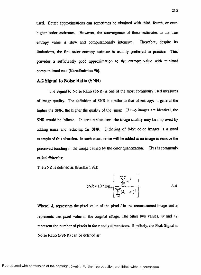
210
used. Better approximations can sometimes be obtained with third, fourth, or even
higher order estimates. However, the convergence of these estimates to the true
entropy value is slow and computationally intensive. Therefore, despite its
limitations, the first-order entropy estimate is usually preferred in practice. This
provides a sufficiently good approximation to the entropy value with minimal
computational cost [Karadimitriou 96].
A.2 Signal to Noise Ratio (SNR)
The Signal to Noise Ratio (SNR) is one of the most commonly used measures
of image quality. The definition of SNR is similar to that of entropy; in general the
higher the SNR, the higher the quality of the image. If two images are identical, the
SNR would be infinite. In certain situations, the image quality may be improved by
adding noise and reducing the SNR. Dithering of 8-bit color images is a good
example of this situation. In such cases, noise will be added to an image to remove the
perceived banding in the image caused by the color quantization. This is commonly
called dithering.
The SNR is defined as [Brislawn 92];
SNR = 10* logeio
n . i * n t
S V
~ a , ) :i = i
A.4
Where, a, represents the pixel value of the pixel i in the reconstructed image and a,
represents this pixel value in the original image. The other two values, nx and ny,
represent the number of pixels in the x and y dimensions. Similarly, the Peak Signal to
Noise Ratio (PSNR) can be defined as:
Reproduced with permission of the copyright owner. Further reproduction prohibited without permission.
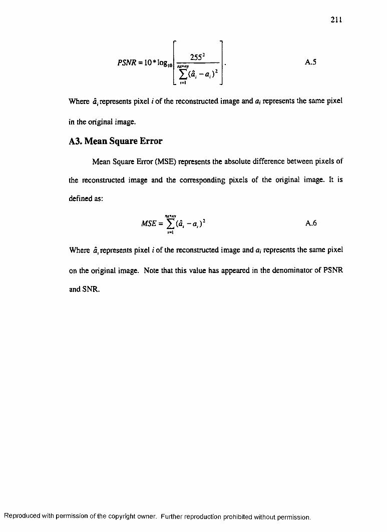
211
PSNR = 10* log 10 A.5nx*ny
Where ai represents pixel i of the reconstructed image and a, represents the same pixel
in the original image.
A3. Mean Square Error
Mean Square Error (MSE) represents the absolute difference between pixels of
the reconstructed image and the corresponding pixels of the original image. It is
defined as:
Where <5, represents pixel i of the reconstructed image and a, represents the same pixel
on the original image. Note that this value has appeared in the denominator of PSNR
and SNR.
M S E = £ ( a t - a t ) z A.6
Reproduced with permission of the copyright owner. Further reproduction prohibited without permission.

APPENDIX B
MRI AND CT IMAGES USED
0
t * v *
Figure (B.l) - The ca MRI brain images
■
Figure (B.2) - The cs MRI brain images
212
Reproduced with permission of the copyright owner. Further reproduction prohibited without permission.

213
o
Figure (B.3) - The bs MRI brain images
:
Figure (B.4) - The bt MRI brain images
Reproduced with permission of the copyright owner. Further reproduction prohibited without permission.

Figure (B.5) - The as MRI brain images
Figure fB.6) - The at MR I brain images
Reproduced with permission of the copyright owner. Further reproduction prohibited without permission.

215
Figure (B.71 - The eb MRI brain images
Figure (B.8) - The es MR I brain images
Reproduced with permission of the copyright owner. Further reproduction prohibited without permission.
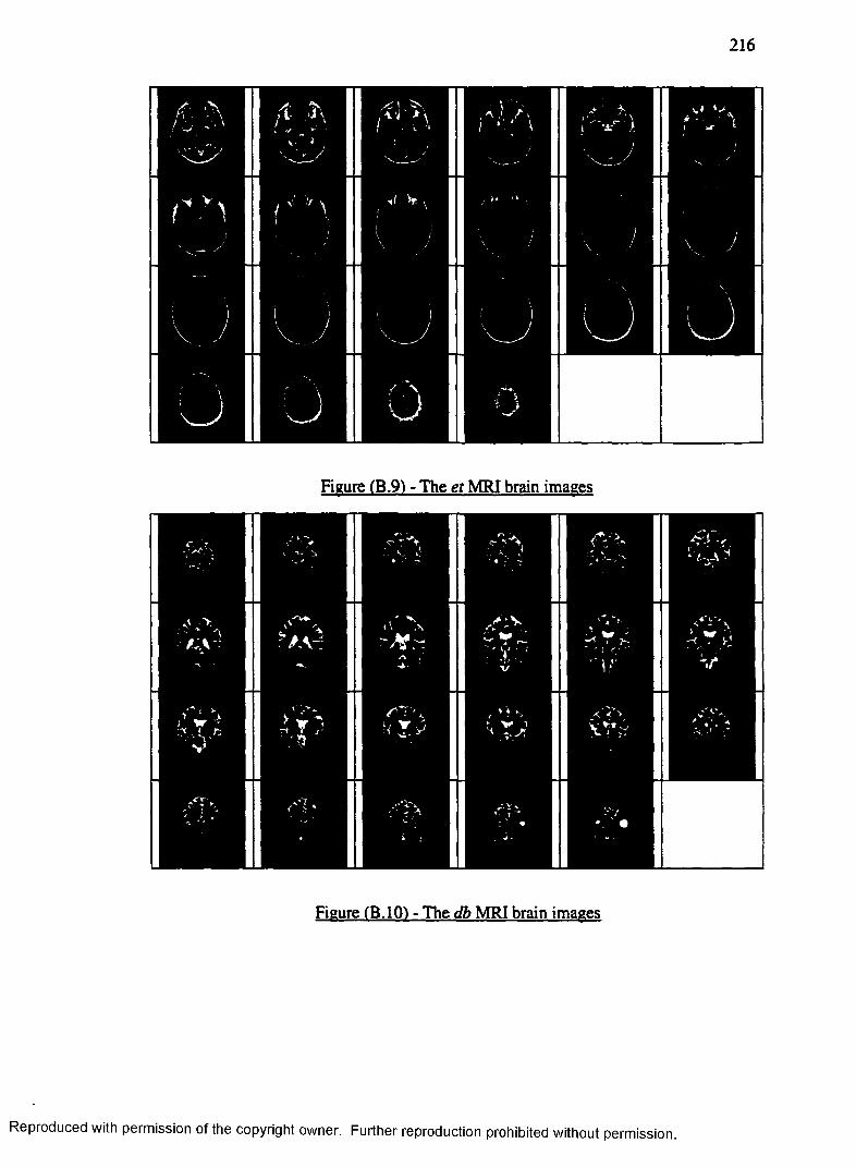
I .
H
i
n
Figure (B.9) - The et MRI brain images
i‘- 7~ ^
< ' Nv w ' i r<- ^'./*
' *
Figure (B.10) - The db MRI brain images
Reproduced with permission of the copyright owner. Further reproduction prohibited without permission.

217
Figure (B.l 1) - The ds MRI brain images
*\
v _ y
\
U
Figure (B.12) - The dt MRI brain images
Reproduced with permission of the copyright owner. Further reproduction prohibited without permission.

218
/, . o^.
" V ’ *. ' .*•
a* A+ , < V-" - -
< u ?
s
/s,4
>< \ 3„
V . /
"J
w -
"1 -- '
— /
B 9fl
M
1
'V A o ’ ")
*v S '
, I 1'
f H
m■■BBB1BB3B1BBKjH■
■ i '
A. S
<r. ,?v
'v
\
Figure (B.13) - The cc CT brain images
Reproduced with permission of the copyright owner. Further reproduction prohibited without permission.
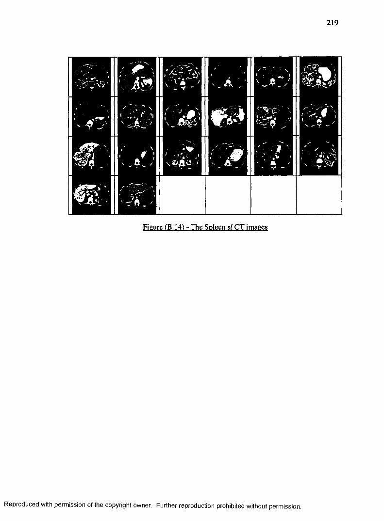
219
'
Figure (B.14) - The Spleen si CT images
Reproduced with permission of the copyright owner. Further reproduction prohibited without permission.

APPENDIX C
HOTELLING TRANSFORM
Hotelling Transform is often referred to as Principal Component Analysis
(PCA), Discrete Karhunen-Loeve transform, or the eigenvector transform [Gonzalez
92]. This transform can represent a set of images as a set of orthonormal principal
component images. These image components contain a specific uncorrelated contrast
mechanism [Newbury 96]. This transform is based on statistical properties of vector
representations. Due to its unique properties, this transform plays an important role in
image processing. Suppose we have a set of N images written as one dimensional
arrays, .t/,X2 xs, in the following form:
The average pixel value of the /th pixel of N images of the set (mean /th pixel value, or
expected value for the /th pixel) can be computed as;
N
XX = C.l
M x = £ { * } = ----* M
C.2
The covariance matrix of the set of images is defined as;
Cx = E [ ( X - M x ) ( X - M x )T} = C.3N
220
Reproduced with permission of the copyright owner. Further reproduction prohibited without permission.

221
Cx is an N*N matrix. In these matrices, the ciy represents the covariance between
pixels x t and x, of the images in the set. In general, Cx is real and symmetric, thus for
the two uncorrelated pixels, x, and Xj the covariance is zero: c,y = cy, = 0.
Since Cx is real and symmetric, there always exists a set of N orthonormal
eigenvectors. Suppose e, are the eigenvectors and A,,i = 1,2 N , are the
corresponding eigenvalues of Cx. These eigenvalues and eigenvectors satisfy the
following:
Ce, =^,e, fori = 1,2,3 N. C.3
The eigenvalues are arranged in an descending order so that;
for y = l,2......... N - 1 C.4
Suppose, A is a matrix with the eigenvectors Cx on its rows. These rows are
ordered in such a way that the eigenvector corresponding to the largest eigenvalue is
on the first row and that of the smallest eigenvalue is on the last row. Suppose A is
used in the following transformation matrix to map the x’s into new vectors denoted as
v’s. This transformation is known as the Hotelling transform and results in a new
coordinate system with the origin at the center of the set and its axes in the direction
of the eigenvectors of Cx, see Figure (C-la). Thus, the transformation is a rotational
transformation that aligns the data with the eigenvectors. This is basically the
mechanism of decorrelating the data, see Figure (C-lb).
The concept of aligning a 2-D image with its principal eigenvectors plays an
important role in image processing. The computer techniques used for image
recognition are sensitive to object rotation. Thus, aligning the image with its principal
Reproduced with permission of the copyright owner. Further reproduction prohibited without permission.

222
eigenvectors, is an effective method for removing the rotational effects from the image
processing procedure.
* ‘I
y i
Fieure(C-D - fa) an rectangle with its principal axes (eigenvectors): (b) rectangle rotated bv using the above transform.
Y = A ( X - M x ) C.5
It can be shown that the mean of Y, E(Y) - My - 0 and the covariance matrix
of y’s can be computed as:
CY = ACxAr . C.6
The eigenvalues are the elements along the diagonal of the diagonal matrix Cx'.
' 4
Cy =A, C.7
In this matrix, CV, all the off diagonal elements are 0, so the elements of the matrix Y
are uncorrelated. It should be noted that both Cx and Cy have the same eigenvalues
and eigenvectors.
Reproduced with permission of the copyright owner. Further reproduction prohibited without permission.

223
A very important application of the Hotelling transform is in the reconstruction
of X from Y Since the rows of A are orthonormal vectors , A'1 is the same as AT.
Thus, any image X can be reconstructed from its corresponding Y. The reconstruction
process is shown as:
X = A t Y + M x . C.8
If all the eigenvalues are used in the above process, perfect reconstruction will result.
However, when fewer eigenvalues, commonly the largest, are used, some error will be
introduced. Suppose, the K largest eigenvalues are used, then eigenvectors of Cx form
the Ax matrix with K eigenvectors. The transformation matrix becomes a K*N matrix
and the Y vector becomes K dimensional. The reconstruction process will not result
in the exact reconstruction of X and can be written as:
X = A tkY + M x . C.9
The mean square error between jcand x is given by:
1 4 • c .iot s l i= l t= K+\
It is observed that the error can be reduced by selecting the K eigenvectors associated
with the largest eigenvalues. It is also evident that this error would be zero when all
eigenvectors are considered.
Example:
Reconstruction of images of a set using the most significant eigenvectors is a good
example for Hotelling transform applications. For this purpose six brain MRI images
shown in Figure (C-2) are used. These six images have 256x256 resolution and will
make a the X matrix of 65536x6 size.
Reproduced with permission of the copyright owner. Further reproduction prohibited without permission.
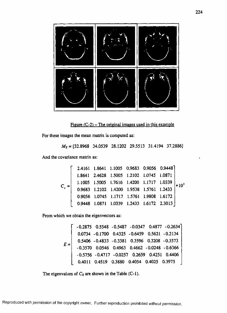
Figure (C-2) - The original images used in this example
For these images the mean matrix is computed as:
Mx = [32.8968 34.0539 28.1202 29.5513 31.4194 37.2886]
And the covariance matrix as:
2.4161 1.8641 1.1005 0.9683 0.9056 0.94481.8641 2.4628 1.5005 1 .2 1 0 2 1.0745 1.08711.1005 1.5005 1.7616 1.4200 1.1717 1.03390.9683 1 .2 1 0 2 1.4200 1.9538 1.5761 1.24330.9056 1.0745 1.1717 1.5761 1.9808 1.61720.9448 1.0871 1.0339 1.2433 1.6172 2.3013
From which we obtain the eigenvectors as:
-0.2875 0.5548 -0.5487 -0.0347 0.4877 -0.26340.0734 -0.1700 0.4325 -0.6459 0.5621 -0.21340.5406 -0.4833 -0.3381 0.3596 0.3208 -0.3573-0.3570 0.0546 0.4963 0.4662 -0.0248 -0.6366-0.5756 -0.4717 -0.0257 0.2659 0.4251 0.44060.4011 0.4519 0.3880 0.4054 0.4025 0.3975
The eigenvalues of Cx are shown in the Table (C-l).
Reproduced with permission of the copyright owner. Further reproduction prohibited without permission.

* 225
Tabe (C-l) - Eigenvalues for the 6 images
•3 *4 •5
250.6 365.7 617.9 1084.3 2153.3 8404.5
Note the dominance of the last 3 eigenvalues. Using (C.9) we have generated the Y
vectors corresponding to the X vectors. Then, we obtained the six principal
component images. The first component image was formed from all the yt
components of the transformed images, and so on for the other images of the set. In
this process, v/ is obtained by performing the inner product of the first row of A with
• .4 V r v
A v . ' /
Figure (C-3) - The six principal component images
the column vector (X - Af*)T. The last row of the matrix A is the eigenvector
corresponding to the largest eigenvalue of the covariance matrix of the image set.
Reproduced with permission of the copyright owner. Further reproduction prohibited without permission.

226
Figure (C-41 - Reconstructed images using all eigenvalues
Figure (C-5) - Reconstructed images using 3 largest eigenvalues
This eigenvalue gives the variance of the gray levels of the last transferred image. The
image transferred using the highest eigenvalue should have the highest contrast. This
Reproduced with permission of the copyright owner. Further reproduction prohibited without permission.

is evident on the Figure (C-3) where the last image has the highest contrast. Note that
when all eigenvalues are used, perfect reconstruction was possible, see Figure (C-4).
However, when the last 3 highest eigenvalues were used the result was different.
Figure (C-6 ) shows the difference between the original image and the reconstructed
image using 3 highest eigenvalues.
Figure (C-6 ) - Difference between the original images and estimated images using 3highest eigenvalues
Reproduced with permission of the copyright owner. Further reproduction prohibited without permission.

APPENDIX D
STATISTICAL ANALYSIS TO DETERMINE THE IMAGE SAMPLE SIZE
D .l Introduction
In science and engineering, there are times that one needs to estimate the
parameters used in a experiment. In such cases, a random sample of the desired
parameter will be used to represent the actual population of the parameter. This
process is often referred to as a random sampling process [Breiman 73]. Reasonable
questions are: "Where can we use this method?" and "What is a good sample size?"
D.2 Random Sample
A random sample is one in which all the observations are statistically
independent under the same distribution. In statistical techniques, a random sample is
usually a sample in which all the observations are statistically independent and
identically distributed [Vining 98].
Suppose we are taking a series of random samples of size n from some
population of y’s. We can compute the sample mean, y :
i . v .y = — d . i
n n tl*
When a large number of samples, n, is used, the sample mean is a good estimate of the
true y and allows us to answer some questions about y. In D.l, since y's are random
variables, then y's are also random variables. The standard deviation for the original
population is denoted as a and standard deviation of sampling distribution of y's is
228
Reproduced with permission of the copyright owner. Further reproduction prohibited without permission.

229
denoted as G-. The second standard deviation <yy is usually referred to as standard
error of the mean. It can be shown that:
a - = 4 = - D.2V f n
The expected value of these samples must be the same as the population mean:
E{y) = n . D.3
When the original population has a normal distribution, then y also follows a normal
distribution with mean (i and standard error <x?. In real life, we may not see a
population in its entirety. As a result, the parameter that describes the important
features of a population is never truly known. However, we can appeal to the Central
Limit Theorem [Vining 98].
D.3 The Central Limit Theorem
Suppose we have a series of random samples each with n observations from a
population with mean n and variance g ~ . If n is sufficiently large, then the sampling
distribution of yis approximately normal. This distribution has a mean of ju and
standard error of G /J n . Using this for a sufficiently large n, we will have:
l z £ = y ^ L ' DA(Ty <j/Vn
This follows a standard normal distribution and for a normal distribution, n=l is
sufficiently large. For a “well behaved” distribution, when the population is
symmetric and have a single peak and the tails die out rapidly, then n = 3 or 5 is a
sufficiently large number. Some literature suggest that n = 6 to 12 are sufficiently
large for a uniform distribution. A uniform distribution does not have a peak, but it is
Reproduced with permission of the copyright owner. Further reproduction prohibited without permission.

230
symmetric and its tails die rapidly, so we still use the Central Limit Unit for it. Some
texts suggest that rt > 30 is a sufficiently large number to assume the Central Limit
Theorem. In general, there are counterexamples to this argument. It is always true
that the more the shape of the distribution deviates from the bell-shaped curve, the
more sample size, n, is required to assume Central Limit Theorem [Vinimg 98].
D.4 Confidence Interval
By assuming a random sample from a normal distribution, it can be shown that
the sample mean, y , and the sample variance, s2, are the most precise unbiased
estimators of fi and c r , respectively. Since y and s2 estimate the specific values for
H and <r2, respectively, they are called point estimators. Since the point estimators
estimate only the specific “point”, they suffer a significant limitation. For instance,
since y is a continuous random variable, we have:
This means that the chance the point estimate, y , represents the true value, pt,
is zero. As a result, statisticians prefer an interval estimate for the parameter. In an
ideal case, the width of an interval represents:
1) The confidence that we have in the interval, and
2) The variability that we may observe in the estimator.
If the sample size, n, is sufficiently large, then y follows a normal distribution
with mean n and standard error a ly fn . Suppose we randomly select two y ’s from
the distribution, then we can construct an interval:
P ( y = M) = 0 . D.5
a D.6
Reproduced with permission of the copyright owner. Further reproduction prohibited without permission.

231
where za denotes the z-value associated with the "tail" area of the standard
normal distribution. For example z002J means z : P(z < z0 02J) = 1.0 - 0.025 = 0.975.
The two possibilities for yare shown on Figure (D.l). In general, only a *100% of
the time one may find// in the lower interval. Under a wide range of conditions, the
population variance:
D . lsf-Jn
follows a /-distribution. The basic confidence interval, ( l-a )* l0 0 % , for//can be
computed:
t — frf/.a/l) — P(~t<lf.al2 — I— —S / j i t
s w ! - r > D-8Vn v«
= P ( y - ' d f .an. ~ r= - y ~ m - y + t * * , 2 ~~r= ^Vn yJn
V
V
Figure (D.l) - Illustration of Confidence Intervals TVining 981
Reproduced with permission of the copyright owner. Further reproduction prohibited without permission.

232
The factor /^ ff/; is the value from the /-table corresponding to a right-hand tail area of
a ! 2 for a /-distribution with d f degrees of freedom. Most statistics books include a
/-table. After repeating this process an infinite number of times with ( 1 - a ) * 100 %
chance, the interval:
y ± W ~ r 0 9vn
would contain the true value for / / . Thus, a (1 - a) * 100% confidence interval for// is:
y ± w f - 0 1 0Vn
The width of this interval reflects:
1) The confidence that we have in the interval through tdf al2, and
2) The variability that the estimator presents through s t j n .
In the case that we know <r: , zrf/ a /: is essentially z0/;and the interval can be defined
as:
7 ± w r D U
The confidence interval represents a reasonable or plausible range of values for the
desired parameter [Vining 98].
D.5 Calculating Sample Sizes
In science and engineering, sometimes we collect data to estimate a parameter
within a given precision. In such cases, a reasonable question is: How many samples
do we use to obtain the desired precision? Using the above procedure, we can find the
sample size only if we have a reasonable idea of the populations standard deviation,
Reproduced with permission of the copyright owner. Further reproduction prohibited without permission.

233
a . Once we have a we can use D.l 1 to compute n. As one can observe in D. 11, the
known), then by changing n we can change the width of the interval. Suppose we set
the mean to be within ± D units, then we can write:
This entire procedure assumes that n is sufficient for the Central Limit
Theorem . Thus, we need the shape of the distribution before determing the
appropriate sample size. Often, the baseline data are used to obtain an estimate fora .
The normal probability plot of the baseline data will provide significant information
about an appropriate sample size required for the Central Limit Theorem. In general,
our samples rarely a have true normal distribution, but for a large enough sample size,
we can still apply to this theorem.
D.6 Random Effects
In experiment-based research, we may have several independent variables
affecting the dependent variable(s). Sometimes, for some independent variables the
levels or the changes are determined by values that are set by the experimenter.
These parameters are said to have fixed effects. There is another class of variables
whose levels are assumed to be randomly selected from an infinite population of
possible levels. These variables are said to have random effects. Researchers are
interested in the random effects and most studies have been done to determine these
term <7 / Vn controls the width of this interval. But, since O’is fixed (assumed to be
D.12
From D.12, n can be computed:
D.13
Reproduced with permission of the copyright owner. Further reproduction prohibited without permission.

234
effects [StatSoft 99]. In this dissertation, we have some dependent variables
(responses) which are affected by independent variables (inputs). In order to
determine where/ how a statistical method could be used these, variables must be
examined.
An objective is to find an optimal wavelet basis to better represent medical
images. Initially, measures of quality for our selection were the Peak Signal to Noise
Ratio (PSNR), Mean Square Error (MSE), and entropy. PSNR and MSE were
measured after the image was reconstructed and entropy was computed from the
wavelet coefficient set representing the image. Because wavelets are used to represent
medical images and this must result in perfect reconstruction of these images, many
wavelets had to be eliminated. Only wavelets, that produce perfect reconstruction,
can be used, i.e., MSE = 0. Since MSE is the denominator of PSNR, PSNR is infinite.
Only the entropy can be the measure of quality and becomes the dependent variable.
We did not use a statistical (random) process for the wavelet basis selection. This
selection was deterministic and based on which wavelets resulted in perfect
reconstruction. Then the best wavelet selection was based on only the entropy, also
deterministic. Once a wavelet was determined, the only independent variable that
affects the entropy is the image. The entropy of wavelet coefficients for different
images varies. In summary, the number of wavelets that produce perfect
reconstruction are not a large enough sample to assume a normal distribution. This
wavelet selection process is not statistical but based solely on the perfect
reconstruction criteria. The only other known parameter for statistical analysis is the
image. This can determine a sample size (number of images) required to produce a
Reproduced with permission of the copyright owner. Further reproduction prohibited without permission.

235
mean entropy value within a specific interval with confidence. A sample size, using
this method, does not produce the number of images required to determine the best
basis. A process for selecting the best basis is presented in Chapter (5).
D.7 A Case Study
Suppose, we have a large enough number of images that have been wavelet-
transformed and we want to determine the number of images, n, required to observe
the entropy in a particular interval with a certain level of confidence. To determine
the sample size, we assume that we have already determined the wavelet w that
produces perfect reconstruction. We further assume this wavelet vv has transformed a
set of MRI brain images producing wavelet coefficient sets, X, for these images.
Assuming the size of set X is large enough, then we can statistically determine the
number of images required such that by some a% confidence, the mean entropy is
within some interval. To demonstrate how this method can be used to find a sample
size for the purpose of illustration, but not to determine the best wavelet nor the
number of images, follows.
D.8 Results
In order to create a sample for this experiment, three MRI-sets (Appendix C:
eb, es, and et) with a total of 69 images were used. Table (D-l), Table (D-2), Table
(D-3), and Table (D-3) present this data.
Reproduced with permission of the copyright owner. Further reproduction prohibited without permission.

236
Table(D-l) - Entropy of wavelet coefficients (perfect reconstruction - best entropy)
Bi44 Bi55 Bi68 Bi44(cont) Bi55(cont) Bi68(cont)4.024285 4.020769 4.046535 4.274402 4.315882 4.3004454.024285 4.020769 4.046535 4.347369 4.392579 4.3743274.150840 4.154868 4.182512 4.205028 4.226751 4.2351904.381064 4.399401 4.411104 3.783106 3.817428 3.8114104.375966 4.377408 4.406029 4.154171 4.199832 4.1885234.485085 4.485926 4.507977 3.713814 3.760834 3.7480304.493417 4.490915 4.523466 3.581121 3.625106 3.6106534.548332 4.545401 4.576327 3.838539 3.878956 3.8545144.536735 4.544195 4.564221 3.799371 3.846564 3.8294684.511857 4.508926 4.545236 3.835537 3.878418 3.8660844.690402 4.695478 4.726795 3.700794 3.735699 3.7347444.652747 4.652764 4.681400 5.331828 5.334608 5.3572974.649533 4.645641 4.683998 5.331828 5.334608 5.3572974.708627 4.707720 4.748346 5.314903 5.317164 5.3448384.629831 4.630384 4.659896 5.337865 5.345398 5.3612004.396842 4.387383 4.426648 5.254790 5.263620 5.2887844.449785 4.446968 4.478289 5.340888 5.340635 5.3597114.477911 4.473964 4.497778 5.176018 5.177321 5.2023504.496702 4.509885 4.527786 5.163643 5.168395 5.1927224.438446 4.434695 4.460828 5.180043 5.174532 5.2113024.276708 4.271671 4.307801 5.239443 5.228885 5.2623314.189906 4.189629 4.216303 5.247498 5.245592 5.269538 .3.648751 3.683130 3.673319 5.173116 5.165596 5.1892103.648751 3.683130 3.673319 5.302807 5.306518 5.3271953.615239 3.656180 3.652879 5.313137 5.299219 5.3355863.794795 3.819029 3.815674 5.267427 5.262200 5.2914764.129997 4.161516 4.162088 5.059032 5.056463 5.0807274.135265 4.164475 4.169713 5.131509 5.107919 5.1523354.113546 4.147572 4.155557 5.317391 5.313519 5.3396874.067583 4.116548 4.108604 5.296671 5.286374 5.3183634.245484 4.276780 4.288502 5.136178 5.123652 5.1512944.432425 4.480376 4.475336 5.049643 5.030255 5.0677234.136822 4.177055 4.169986 5.212450 5.202651 5.2279334.303726 4.341145 4.345753 4.976873 4.966710 4.9905694.310810 4.331901 4.340558
Table (D-l) was generated using the entropy of images obtained by three
different perfect reconstruction wavelets. The wavelets presented in Table (D-l)
generated the lowest entropy for all image sets (Chapter (5)). The 69 MRI brain
Reproduced with permission of the copyright owner. Further reproduction prohibited without permission.

237
images used here are images of different "slices" from three different angles and are
from different locations. Table (D-2) presents the statistics of Table (D-1).
Table (D-2) - Statistics for the entropy in Table (D-l)
Wavelet Minimum Maximum Mean STD ( a ) VarianceBi44 3.581121 5.340888 4.544358 0.55507048 0.308Bi55 3.625106 5.345398 4.555992 0.54040657 0.292Bi6 8 3.610653 5.361200 4.572318 0.55236757 0.305
As expected and our results in Chapter (5) showed that these three wavelets
produce similar result. We will use the a from Table (D-l) to estimate the sample
size.
Sample Calculation (1 ): (Bi44 wavelet is used in this part)
Suppose we want to determine the number of MRI brain images in a set such
that with 90% confidence, the mean entropy of the set is in the: 4.544358 ±0.5
interval. This is the same as saying, we want to generate a 90% confidence interval
with a width of ±0.5. Using D .l3 and the z values provided in Appendix (2) [Vining
98]:
n 2 ^ 6 4 5 ^ 5 0 7 0 4 8 3 33
Thus, a sample size of 4 or more images is required to generate the desired confidence
interval. Let’s repeat the same calculation for a confidence interval of 90% with the
smaller width of ±0.2, i.e., intervals of 4.544358 ±0.2. This time we have a
different value for the interval size and :
f 1.645*0.55507048 n> ---- = 20.8 ,0.2
Thus, a sample of 21 or more images is needed to generate this confidence interval.
Reproduced with permission of the copyright owner. Further reproduction prohibited without permission.

238
In the next two examples, we will use a higher confidence level of 98% with
the above two widths. Since the confidence level has changed, we have to use a new z
value corresponding to 98% confidence. For the first case (width ± 0.5):
Thus, with a sample size of 7 or more images, we are able to generate a 98%
confidence interval with a width of ±0.5, i.e., intervals of 4.544358 ±0.5. Similarly,
we can show that:
Thus, with a sample size of 42 or more images, we generate the 98% confidence
interval of 4.544358 ± 0.2.
Sample Calculation (2): (Bi31 wavelet is used in this part)
Table (D-3) presents the entropy of wavelet coefficients for the wavelets that
resulted in perfect reconstruction but the highest entropy. For the illustration purpose,
bi31 wavelet with the highest STD is selected. Since STD appears as the numerator
of D .l3, a larger STD results in a larger sample size. This sample size calculation is
similar to that of the Sample Calculation (1) with a new wavelet. In this case, We
used the statistics provided in Table (D-4) to determine the sample size for the same
interval sizes and confidence levels as those in the previous example. For a 90%
confidence interval with a width of ±0.5: the sample size, n, is:
2.326*0.55507048
f 2.326* 0.55507048 V n > ----------------------- =41.67
1.645*0.67671650
Reproduced with permission of the copyright owner. Further reproduction prohibited without permission.

239
Thus, a sample size of 5 or more images is needed to generate this confidence interval,
i.e., 90% confidence interval for the 5.207654 ±0.5 intervals.
Table(D-3) - Entropy of wavelet coefficients (perfect reconstruction - worst entropy)
Bil3 Bil5 Bi31 Bil3(cont) Bil5(cont.) Bi31(cont)4.379069 4.430151 4.871251 4.802136 4.887201 4.7407074.379069 4.430151 4.871251 4.778417 4.859244 4.7153124.560225 4.620262 4.972686 4.832935 4.910732 4.7952194.849756 4.913314 5.140932 4.686905 4.775200 4.6594074.899639 4.959822 5.096913 4.294822 4.364969 4.2331275.029729 5.085098 5.168891 4.661065 4.734231 4.6084855.038622 5.098197 5.176796 4.220282 4.287312 4.1689395.088439 5.146761 5.223077 4.067629 4.159214 4.0604165.081956 5.152997 5.222972 4.285049 4.362047 4.3244555.050016 5.120349 5.165433 4.233131 4.303348 4.3061125.240058 5.309336 5.370975 4.235038 4.295108 4.3625085.215342 5.284121 5.316204 4.046308 4.119415 4.2841625.199251 5.257512 5.318776 5.746172 5.805668 6.0629885.258077 5.312083 5.376130 5.733561 5.796314 6.0563225.161620 5.223582 5.316609 5.750403 5.827701 6.0824924.933657 5.001229 5.059169 5.660399 5.720887 6.0188034.989996 5.054486 5.109312 5.712933 5.776192 6.1100924.999333 5.059279 5.142894 5.559908 5.606962 5.9513855.014323 5.077599 5.198678 5.549496 5.593971 5.9636534.938874 4.994572 5.153639 5.541899 5.599775 5.9815814.741042 4.799689 5.034823 5.615614 5.685324 6.0368014.592625 4.655317 4.997394 5.608656 5.660113 6.0528124.380873 4.431309 4.884020 5.506454 5.569029 6.0046274.063635 4.126199 4.205608 5.653632 5.706145 6.1292314.063635 4.126199 4.205608 5.654165 5.711994 6.1317664.065755 4.128537 4.137080 5.607700 5.659856 6.1140434.228433 4.294593 4.275524 5.409392 5.472589 5.9114424.573999 4.639157 4.579826 5.465524 5.518778 5.9799904.607298 4.683074 4.575369 5.637889 5.699725 6.1735604.622346 4.690404 4.557779 5.613484 5.664282 6.1628624.563941 4.626338 4.508058 5.425201 5.472534 6.0134874.715820 4.792841 4.677086 5.302451 5.367500 5.9616134.899252 4.975430 4.876488 5.432535 5.489659 6.1950964.627249 4.697908 4.580624 5.165655 5.219322 6.0023224.790817 4.871153 4.749108
Reproduced with permission of the copyright owner. Further reproduction prohibited without permission.

240
Table (D4) - Statistics of the entropy presented in Table (D3)
Wavelet Minimum Maximum Mean STD (<t) VarianceBil3 4.046308 5.750403 4.972668 0.52253343 0.273Bil5 4.119415 5.827701 5.036529 0.51887474 0.269Bi31 4.060416 6.195096 5.207654 0.67671650 0.458
For a 90% confidence interval of width ±0.2, n is:
' 1.645 *0.67671650 Vn > = 30.98,
0.2 JThus, with a sample size of 31 or more, we are able to generate the 90% confidence
interval with 5.207654 ±0.2 intervals.
In the next two examples, we will use a higher confidence level of 98%. To
generate a 98% confidence interval of width ±0.5, we need:
n a r 2.326 ♦ 0^6767 ‘650 ) 3 = g 9
Thus, with a sample size of 10 or more we generate the 98% confidence interval for
the 5.207654 ±0.5 intervals. Similarly, to generate a 98% confidence interval with a
width of ± 0.2, we need a sample size, n:
f 2.326 *0.67671650 V n> ------------------------- =61.9,I 0 .2 J
Thus, with a sample size of 62 or more images we will generate a 98% confidence
interval for 5.207654 ±0.2 intervals.
These results are interesting, however with respect to the objectives of this
dissertation, they may not be significant. Perhaps estimating the entropy of an image
set will be useful in estimating the disk space required for saving the set after an
entropy-based compression. In this dissertation, we have set some criteria to select
Reproduced with permission of the copyright owner. Further reproduction prohibited without permission.

241
some wavelets that better represent medical images. Due to the set criteria (perfect
reconstruction, i.e., MSE = 0, and PSNR = infinity), the selection of wavelet was not a
random process. The only random variables that affect the entropy are the images
themselves. Note that we have used entropy as the measure of quality (dependent
variable) here. The reason for such a selection is that after selecting the wavelets that
generate perfect images both MSE and PSNR no longer vary. Thus, selection of the
best wavelet base from among the remaining wavelets is based on the entropy. In the
2-step selection process, the wavelet that resulted in a better compression from among
the one capable of generating perfect images was selected as the best base to carry on
the research. The 2-step selection process was not a statistical process.
An important observation made in Table (D-i) and Table (D-4) is that, the
overall mean values of entropy for the best wavelets in Table (D-l) are lower than
those of the worst wavelets in Table (D-l). Note that all the wavelets discussed here
resulted in perfect reconstruction. Another interesting observation is that there is not
much difference between the sample sizes predicted by the best and worst wavelets.
Reproduced with permission of the copyright owner. Further reproduction prohibited without permission.

VITA
Rahman Tashakkori was bom on May 24, 1963 in Jahrom, Iran. He received
his high-school diploma from Khajeh-Naseer Tousee high-school in 1981. He
graduated with the bachelor of science degree in physics from Shahid Chamran
University in Ahwaz, Iran, in August, 1987. Rahman received two master of science
degrees from Louisiana State University, the first one in nuclear engineering in May
1994, and the second one in Engineering Science/System Science in December 1995.
He is currently a doctoral degree candidate in the Department of Computer Science at
Louisiana State University.
Rahman is married to Sharareh Nikbakht, and has two children, a girl named
Parisa and a boy named Sina. Rahman is currently working as an instructor in the
Department of Computer Science at the Appalachian State University in Boone, North
Carolina.
242
Reproduced with permission of the copyright owner. Further reproduction prohibited without permission.

DOCTORAL EXAMINATION AND DISSERTATION REPORT
Candidates Rahman Tashakkori
Major Field: Computer Science
Title of Dissertation: Medical Image Set Compression Using Wavelet and L iftin gCombined with New Scanning Techniques
rofesso# and
Graduate School
EXAMINING COMMITTEE:
Date of Krani nation:
April 2, 2001
Reproduced with permission of the copyright owner. Further reproduction prohibited without permission.