MEDEA:

a DSGE Model for the Spanish Economy

Pablo Burriel

Oficina Económica del Presidente

Jesús Fernández-Villaverde

University of Pennsylvania, NBER, and CEPR

Juan F. Rubio-Ramírez

Duke University and Federal Reserve Bank of Atlanta

March 9, 2009

1

1. Introduction

In this paper, we describe a Dynamic Equilibrium Model of the Spanish Economy named

MEDEA (Modelo de Equilibrio Dinámico de la Economía EspañolA). This model was de-

veloped while the authors collaborated with the Economic Office of the President of Spain

(Oficina Económica del Presidente del Gobierno).

MEDEA is a dynamic stochastic general equilibrium (DSGE) model that aims to describe

the main features of the Spanish economy for policy analysis, counterfactual exercises, and

forecast. As such, it is a model for a small open economy that belongs to a currency area,

in this case, the Euro. The open economy aspects are captured by the presence of exporting

and importing firms with incomplete pass-through and by the ability of the agents to save

or borrow on foreing financial assets. The currency area is modelled through a monetary

authority that sets short-term nominal interest rates by following a Taylor rule based on the

economic performance of the whole Euro area.

MEDEA is built in the tradition of New Keynesian models with real and nominal rigidities

(see Christiano, Eichenbaum, and Evans, 2005, Smets and Wouters, 2003, and the book-

length description in Woodford, 2003). The New Keynesian models have demonstrated to be

a flexible framework that can incorporate many different economic mechanisms of interest, to

be rich enough for meaningful policy analysis, and with a good forecasting performance track.

At the kernel of MEDEA, we have a neoclassical growth model with optimizing households

and firms and long-run growth induced by technological change and population growth. On

top of this core, MEDEA has rigidities of prices and wages, a set of adjustment costs (to

investment, to exports, and to imports), a fiscal and monetary authority that determines a

short run nominal interest rate and taxes, and shocks to technology, preferences, and policy

that induce the stochastic dynamics of the economy.

MEDEA, shares many features with other DSGE models developed at policy-making

institutions to use them as an input for their activities. Some examples are the Federal

Reserve Board (Erceg, Guerrieri, and Gust, 2005), the European Central Bank (Christoffel,

Coenen, and Warne, 2007), the Bank of Canada (Murchison and Rennison, 2006), the Bank

of England (Harrison et al., 2005), the Bank of Findland (Kilponen and Ripatti, 2006 and

Kortelainen, 2002), the Bank of Sweden (Adolfson et al., 2005) the Bank of Spain (Andrés,

Burriel and Estrada, 2006), and the Ministerio de Economía y Hacienda (Boscá et al (2007)).

However, it also has many new features, some that are in our opinion interesting advances

for DSGE modelling in general, and some that are important to adapt the model to Spain.

We would like to highlight:

1. MEDEA has stochastic growth coming from three sources: general technological progress,

2

investment specific technological progress and population growth. These will allow us

to capture two relevant characteristics of Spain in the last decade: the low productivity

growth and the large rise in immigration.

2. In comparison with other recent estimated DSGE models, we do not model the foreign

world as an equilibrium outcome beyond the behavior of the European Central Bank

through its the Taylor rule. Spain is too small to be of significant impact to the wold

economy. We prefer to use the extra complexity in other aspects of the model.

3. Fiscal policy. Most of the estimated DSGE models have been developed in central

banks. As it corresponds to their role, central banks have paid particular attention to

issues related with monetary policy but the treatment of fiscal policy has been very

parsimonious. We pay a more detailed attention to the fiscal sector of the economy,

with three different tax tates, on capital income, labor income, and consumption.

4. At a more technical level, we design the solution of the model in such a way that we

will be able to undertake higher order approximations in the middle run in a relatively

simple way. There is a growing body of literature that emphasizes that there is much

to be gained from a nonlinear estimation of the model, both in terms of accuracy and in

terms of identification (see Fernández-Villaverde and Rubio-Ramírez, 2006, Fernández-

Villaverde, Rubio-Ramírez, and Santos, 2006, and An and Schorfheide, 2006, among

several others). In the current version of the model, because of computational reasons,

we solve the model by log-linearizating the equilibrium conditions around a transformed

stationary steady-state.

MEDEA is estimated by Bayesian methods. We follow the Bayesian paradigm because

it is a powerful, coherent, and flexible perspective for the estimation of dynamic models in

economics (see An and Schorfheide, 2006, for an excellent survey). First, Bayesian analysis

is built on a clear set of axioms and it has a direct link with decision theory. The link is

particularly relevant for MEDEA since the model will be used for policy analysis. Many of

the relevant policy decisions require an explicit consideration of uncertainty and asymmetric

risk assessments. Consequently, the Bayesian approach provides a convenient playground

for risk management. Second, the Bayesian approach deals in a transparent way with mis-

specification and identification problems, which are pervasive in the estimation of DSGE

models (Canova and Sala, 2006, and Iskrev, 2007). Third, the Bayesian estimators have

desirable small sample and asymptotic properties, even if they are evaluated by classical cri-

teria (Fernández-Villaverde and Rubio-Ramírez, 2004). Fourth, priors allow us to introduce

presample information and to reduce the dimensionality problem associated with the number

3

of parameters. As Sims (2007) has emphasized, with any model rich enough to fit the data

well, the use of priors is essential to do any reasonable inference. Priors will be especially

attractive for MEDEA because the deep changes in the structure of the spanish economy

over the last decades stops us from using data before the early 1980s, leaving us with a rel-

atively short sample. Finally, Bayesian methods have important computational advantages

over maximum likelihood in large models like MEDEA. Simulating the posterior distribution

of the parameters is a much easier task than to maximize the likelihood.

MEDEA can be employed for two main alternative purposes. First, we can use it to

understand the dynamics of aggregate fluctuations. In this paper we will show a decompose

of the last business cycle among different sources of variation. Second, we can use MEDEA

for policy analysis, including counterfactuals and different experiments.

The structure of this paper is as follows. First, we outline the main structure of the model.

Second, we describe MEDEA’s theoretical framework in detail. Third, we define the equilib-

rium of the economy, we transform this equilibrium into a stationary one by appropriately

changing the variables, and we solve the model by loglinearizing the equilibrium conditions

of the transformed model. Fourth, we build the likelihood of the model. Finally, we estimate

the model with data from 1986:1 to 2007:2 and we report the results of a number of exercises

undertaken with the model.

2. Outline of the Model

The basic structure of the model is as follows:

1. A continuum of households consume, save in domestic and foreign assets, hold money,

supply labor, and set their own wages subject to a demand curve and Calvo’s pricing

with partial indexation.

2. The labor of households is aggregated by a perfectly competitive labor packer who sells

the aggregated labor to the domestic intermediate good producers.

3. The final domestic good is manufactured by a final domestic good producer, which uses

as inputs intermediate domestic goods.

4. The consumption good is packed by a consumption good producer using the final do-

mestic good and the final imported good.

5. Similarly, the investment good is packed by an investment good producer using the final

domestic good and the final imported good.

4

6. Domestic intermediate goods producers rent capital and labor to manufacture their

good and are subject to Calvo’s pricing with partial indexation.

7. The final imported good is packed by a final imported good producer using interme-

diate goods produced by monopolistic competitors from a generic import good, with

incomplete pass-through specified as Calvo’s pricing with partial indexation.

8. The export goods are produced by monopolistic competitors who buy the final domestic

good and differentiate it by brand naming. The exporters exhibit local-currency pricing

that we specify as Calvo’s pricing with partial indexation.

9. There is a monetary authority, the ECB, that implements monetary policy. The ECB’s

monetary policy fixes the one-period nominal interest rate of the Euro area through

open market operations, with the Euro area inflation as target. The weight of the

Spanish economy in this policy target is approximately 10 per cent.

10. There is a government that implements fiscal policy to finance an exogenously given

stream of government consumption with taxes on capital and labor income and on

consumption.

11. Finally, long run growth of per capita income is induced by the presence of two unit

roots, one in the level of neutral technology and one in the investment-specific technol-

ogy. Moreover, there is population growth.

3. The Model

3.1. Households

There is a continuum of households indexed by j ∈ [0, 1]. Each household is composed by Lt

identical workers. The preferences of households are representable by the following lifetime

utility function, which is separable in per capita consumption, cjt, per capita real money

balances, mjt/pt (where pt is the price of the domestic final good), and per capita hours

worked, lsjt (in terms of proportion of the period spent at work):

E0∞Xt=0

βtLtdt

(log (cjt − hcjt−1) + υ log

mjt

pt− ϕtψ

¡lsjt¢1+ϑ

1 + ϑ

)

where E0 is the conditional expectation operator evaluted at time 0, β is the discount factor,h is the parameter that controls habit persistence, and ϑ is the inverse of Frisch labor supply

5

elasticity. The variable dt is an intertemporal preference shock, while ϕt is a labor supply

shock with laws of motion:

log dt = ρd log dt−1 + σdεd,t where εd,t ∼ N (0, 1),logϕt = ρϕ logϕt−1 + σϕεϕ,t where εϕ,t ∼ N (0, 1).

Note that the preference shifters are common for all households. The preference shock dt

will change the intertemporal first order conditions, while the preference shock ϕt will change

the first order conditions affecting labor supply and wage determination. We include the

shock dt to capture the changes in valuations between the present and the future that the

analysis of intertemporal wedges suggests as key for understanding aggregate fluctuations (see

Primeri, Schaumburg, and Tambalotti, 2005). We add the shock ϕt to model the changes

in labor supply that Hall (1997) and Chari, Kehoe, and McGrattan (2005) have pointed out

as responsible for a large proportion of the changes in employment over the business cycle.

We have selected a utility function where consumption appears in logs. Consequently, the

marginal relation of substitution between consumption and leisure is linear in consumption

to ensure the presence of a balanced growth path with constant hours (King, Plosser, and

Rebelo, 1988).

The household’s size, Lt, follows a random walk with drift in logs:

Lt = Lt−1 exp (ΛL + zL,t) where zL,t = σLεL,t and εL,t ∼ N (0, 1).

Thus, the growth of population is given by

γLt =Lt

Lt−1= exp (ΛL + zL,t)

This process induces the first unit root in the model. However, this unit root will only affect

the absolute levels of the variables and not the per capita terms.

Households hold an amount ajt+1 of arrow securities1, an amount bjt of domestic govern-

ment bonds2 that pay a nominal gross interest rate of Rt and an amount in domestic currency

extbWjt of foreign government bonds from the rest of the world, that pay a nominal gross in-

terest rate of RWt Γ (·). The exchange rate, ext, is expressed in terms of the domestic currency

1Households can trade on the whole set of possible Arrow securities, indexed both by the household j(since the household faces idiosyncractic wage-adjustment risk that we will describe below) and by time (tocapture aggregate risk). ajt+1 indicates the amount of those securities that pay one unit of the domestic finalgood in event ωj,t+1,t purchased by household j at time t at a (real) price qjt+1,t.

2These may include government bonds from other countries of EMU.

6

per unit of foreign currency. The function Γ (·) represents the risk premium associated with

buying foreign bonds and it captures the costs for households of undertaking positions in the

international asset market. We will assume that Γ (·) depends on the per capita holdingsof foreign bonds in the entire economy with respect to nominal output of the final domestic

good: ebWt =

R 10bWjt dj

ptydt

Thus, as borrowers, households are charged a premium on the foreign interest rate (i.e., ifebWt < 0 we have Γ³extebWt , ξb

W

t

´< 1) and get a remuneration when they act as lenders.

Moreover, Γ (0) = 1, Γ (·)0 > 0, and Γ (·)00 < 0. Domestic households take ebWt as given when

deciding their optimal holding of foreign bonds. Finally, revenues from the premium are

rebated lump-sum to the foreign agents.3 This cost is introduced to pin down a well-defined

steady-state for consumption and assets in the context of international incomplete markets.4

Since we do not model the rest of the world, the evolution of the RWt is given by:

RWt =

¡RW

¢(1−ρRW ) ¡RWt−1¢ρ

RW e(σRW εRW ,t)

In addition, there is a time varying shock to the risk-premium ξbW

t , with the following process:

log ξbW

t = ρbW log ξbW

t−1 + σbW εbW ,t where εbW ,t ∼ N (0, 1),

With all this structure, the j − th household’s per capita budget constraint is given by:

(1 + τ c)pctptcjt +

pitptijt +

mjt

pt+

bjtpt+

extbWjt

pt+

Zqjt+1,tajt+1dωj,t+1,t

= (1− τw)wjtlsjt +

¡rtujt (1− τk) + μ−1t δτk − μ−1t Φ [ujt]

¢kjt−1 +

1

γLt

mjt−1

pt

+Rt−11

γLt

bjt−1pt

+RWt−1Γ

³extebWt−1, ξbWt−1´ 1

γLt

extbWjt−1

pt+1

γLtajt + Tt +zt

where pt is the price of the domestic final good, pct is the price level of the consumption final

good, pit is the price level of the investment final good, wjt is the real wage in terms of the

domestic final good, rt the real rental price of capital, also in terms of the domestic final

good, ujt > 0 the intensity of use of capital, μ−1t Φ [ujt] is the physical cost of use of capital in

3However, since we do not model the equilibrium behavior of the rest of the world, the way in which thisrebate is distributed is irrelevant for our purposes.

4See Schmitt-Grohé and Uribe (2003) for a detailed discussion on this issue and for alternative modelingchoices.

7

resource terms, μt is an investment-specific technological shock to be described momentarily,

Tt is a lump-sum transfer, zt are the profits of the firms in the economy, and τ c, τw, and τk

are the tax rates on consumption, wages and capital income. Note that the tax on capital

income is defined on the net return of capital after depreciation δ and hence we include a tax

credit μ−1t δτk, expressed in resource terms. Also, note that we divide the per capita holdings

of money and bonds carried into the period by the current population growth to express all

quantities in current population per capita terms. Finally, we assume that Φ [1] = 0, Φ0 and

Φ00 > 0.

Investment ijt induces a law of motion for (per capita) capital of the household:

EtγLt+1kjt = (1− δ) kjt−1 + μt

µ1− S

∙γLt

ijtijt−1

¸¶ijt

where S [·] is an adjustment cost function such that S [Λi] = 0, S0 [Λi] = 0, and S00 [·] > 0 andΛi is the growth rate of investment along the balance growth path. Note our capital timing:

we index capital by the time its level is decided. Also, the amount of per capita capital in

the next period is random because the population next period is also random.

We include an investment-specific technological shock motivated by the evidence of Green-

wood, Herkowitz, and Krusell (1997 and 2000) that have vigorously argued the importance

of this channel to account for growth and aggregate fluctuations. The investment-specific

technological shock follows an autoregressive process:

μt = μt−1 exp (Λμ + zμ,t) where zμ,t = σμεμ,t and εμ,t ∼ N (0, 1)

This process induces a second unit root in the model. The value of μt also determines the

relative price of new capital in terms of the final domestic good:

pitpt

1

μt

Given our description of the household’s problem, the lagrangian function associated with

it is:

E0∞Xt=0

βteγLt

⎡⎢⎢⎢⎢⎢⎢⎢⎢⎢⎣

dt

½log (cjt − hcjt−1) + υ log

mjt

pt− ϕtψ

(lsjt)1+ϑ

1+ϑ

¾

−λjt

⎧⎪⎪⎨⎪⎪⎩(1 + τ c)

pctptcjt +

pitptijt +

mjt

pt+

bjtpt+

extbWjtpt

+Rqjt+1,tajt+1dωj,t+1,t

− (1− τw)wjtlsjt −

¡rtujt (1− τk) + μ−1t δτk − μ−1t Φ [ujt]

¢kjt−1 − 1

γLt

mjt−1pt− Tt −z

−Rt−11γLt

bjt−1pt−RW

t−1Γ³extebWt−1, ξbWt−1´ 1

γLt

extbWjt−1pt− 1

γLtajt

−Qjt

nγLt+1kjt − (1− δ) kjt−1 − μt

³1− S

hγLt

ijtijt−1

i´ijto

8

where eγLt =Yt

i=1γLi and they maximize over cjt, bjt, b

Wjt , ujt, kjt, ijt, mjt, wjt and lsjt; while

λjt and Qjt are the lagrangian multipliers associated with the budget constraint and the

evolution of installed capital, respectively.

The first order conditions of this problem are:

dt (cjt − hcjt−1)−1 − hEtβγLt+1dt+1 (cjt+1 − hcjt)

−1 = λjt (1 + τ c)pctpt

λjt = Etβλjt+1Rt

Πt+1

λjt = Et

⎧⎨⎩βλjt+1RWt Γ

³extebWt , ξb

W

t

´Πt+1

ext+1ext

⎫⎬⎭rt =

μ−1t Φ0 [ujt]

(1− τk)

qjtEtγLt+1 = βEtγLt+1½λjt+1λjt

¡(1− δ) qjt+1 +

¡rt+1ujt+1 (1− τk) + μ−1t+1δτk − μ−1t+1Φ [ujt+1]

¢¢¾pitpt= qjtμt

µ1− S

∙γLt

ijtijt−1

¸− S0

∙γLt

ijtijt−1

¸γLt

ijtijt−1

¶+EtβγLt+1qjt+1

λjt+1λjt

μt+1S0∙γLt+1

ijt+1ijt

¸γLt+1

µijt+1ijt

¶2mjt

pt= dtυ

∙βEtλjt+1

Rt − 1Πt+1

¸−1.

where we have defined the (marginal) Tobin’s Q as qjt =Qjt

λjt, (the ratio of the two lagrangian

multipliers, or more loosely the value of installed capital in terms of its replacement cost),

and substituted the Euler equation into the money balances equation.5

The first order condition with respect to investment has a simple interpretation. If S [·] = 0(i.e., there are no adjustment costs), we get:

qjt =pitpt

1

μt

i.e., the marginal Tobin’s Q is equal to the replacement cost of capital (the relative price of

capital) in terms of the domestic final good. Furthermore, if μt = 1 and pit = pt, as in the

standard neoclassical growth model, qjt = 1.

5We do not take first order conditions with respect to Arrow securities since, in our environment withcomplete markets and separable utility in labor, their equilibrium price will be such that their demand ensuresthat consumption does not depend on idiosyncractic shocks (see Erceg, Henderson, and Levin, 2000).

9

3.1.1. Labor demand and wage decisions:

The first order conditions with respect to labor and wages are more involved. The labor

used by intermediate good producers to be described below is supplied by a representative

competitive firm that hires the labor supplied by each household j, Ltlsjt. The labor supplier

aggregates the differentiated labor types with the following production function:

Ldt = Lt

µZ 1

0

¡lsjt¢ η−1

η dj

¶ ηη−1

= Ltldt (1)

where 0 ≤ η <∞ is the elasticity of substitution among different types of labor and ldt is the

per-capita labor demand (Ldt is the per-household labor demand).

The labor “packer” maximizes profits subject to the production function (1), taking as

given all differentiated labor wages wjt and the aggregate wage wt:

maxljt

wtLtldt −

Z 1

0

wjtLtlsjtdj

whose first order conditions are:

wtη

η − 1

µZ 1

0

¡lsjt¢ η−1

η dj

¶ ηη−1−1 η − 1

η

¡lsjt¢η−1

η−1 − wjt = 0 ∀j

Dividing the first order conditions for two types of labor i and j and integrating over all labor

types we get: Z 1

0

wjtlsjtdj = wit (l

sit)

1η

Z 1

0

¡lsjt¢ η−1

η dj = wit (lsit)

1η¡lsjt¢η−1

η

Using the zero profits condition implied by perfect competition wtldt =

R 10wjtl

sjtdj and solving

we obtain the (per capita) input demand function and aggregate wage:

lsjt =

µwjt

wt

¶−ηldt ∀j

wt =

µZ 1

0

w1−ηjt dj

¶ 11−η

(2)

Idiosyncratic risks come about because households set their wages following a Calvo’s

setting.6 In each period, a fraction 1 − θw of households can change their wages. All other

households can only partially index their wages by past final domestic good inflation. Index-

6We assume that when new workers in the household begin to work they are assigned a wage so that thewage distribution of new entrants replicates exactly the existing wage distribution in the economy.

10

ation is controlled by the parameter χw ∈ [0, 1]. This implies that if the household cannot

change her wage for τ periods her normalized wage after τ periods isτY

s=1

Πχwt+s−1Πt+s

wjt.. The

relevant part of the lagrangian for the household is then:

maxwjt

Et∞Xτ=0

θτwβτeγLτ

(−dt+τϕt+τψ

¡lsjt+τ

¢1+ϑ1 + ϑ

+ λjt+τ

τYs=1

Πχwt+s−1Πt+s

(1− τw)wjtlsjt+τ

)

s.to : lsjt+τ =

ÃτY

s=1

Πχwt+s−1Πt+s

wjt

wt+τ

!−ηldt+τ

All households set the same wage (w∗t = wjt ∀j) because complete markets allow them tohedge the risk of the timing of wage change. Hence, we can drop the jth from the choice of

wages and λjt. The first order condition of this problem is7:

η − 1η

(1− τw)w∗tEt

∞Xτ=0

(βθw)τ eγLτ λt+τ

ÃτY

s=1

Πχwt+s−1Πt+s

!1−η µw∗twt+τ

¶−ηldt+τ =

Et∞Xτ=0

(βθw)τ eγLτ

⎛⎝dt+τϕt+τψ

ÃτY

s=1

Πχwt+s−1Πt+s

w∗twt+τ

!−η(1+ϑ) ¡ldt+τ

¢1+ϑ⎞⎠In order to be able to express this equation recursively we re-label each part of this equality

as f1t and f2t , and add the equality f1t = f2t :

f1t =η − 1η

(1− τw)w∗tEt

∞Xτ=0

(βθw)τ eγLτ λt+τ

ÃτY

s=1

Πχwt+s−1Πt+s

!1−η µwt+τ

w∗t

¶η

ldt+τ

f2t = Et∞Xτ=0

(βθw)τ eγLτ dt+τϕt+τψ

ÃτY

s=1

Πχwt+s−1Πt+s

!−η(1+ϑ)µwt+τ

w∗t

¶η(1+ϑ) ¡ldt+τ

¢1+ϑThen, we express f1t and f2t recursively and since f

1t = f2t , we substitute them by ft, such

that:

ft =η − 1η

(1− τw) (w∗t )1−η λtw

ηt ldt + βθwEtγLt+1

µΠχwt

Πt+1

¶1−η µw∗t+1w∗t

¶η−1ft+1

7Note that for those sums to be well defined (and, more generally for the maximization problem to have

a solution), we need to assume that (βθw)τ eγLτ λt+τ goes to zero faster than

ÃτY

s=1

Πχwt+s/Πt+s−1

!1−ηgoes to

infinity in expectation.

11

and

ft = dtϕtψ

µw∗twt

¶−η(1+ϑ) ¡ldt¢1+ϑ

+ βθwEtγLt+1µΠχwt

Πt+1

¶−η(1+ϑ)µw∗t+1w∗t

¶η(1+ϑ)

ft+1

We need both laws of motion to be able, later, to solve for all the relevant endogenous

variables.

Finally, in a symmetric equilibrium, in every period, a fraction 1− θw of households set

w∗t as their wage, while the remaining fraction θw partially index their price by past inflation.

Consequently, the real wage index evolves:

w1−ηt = θw

µΠχwt−1Πt

¶1−ηw1−ηt−1 + (1− θw)w

∗1−ηt .

i.e., as a geometric average of past real wage and the new optimal wage. This structure is a

direct consequence of the memoriless characteristic of Calvo pricing.

3.2. The Distribution Sector

The distribution sector is composed of two segments. At the end, there is a consumption

good producer and an investment good producer, while at the source, a final domestic good

producer aggregates all domestic intermediate goods to produce the final domestic good.

3.2.1. Final Consumption and Investment Good Producers

At the top of the distribution chain, there is a perfectly competitive consumption and invest-

ment good producer who pack domestic consumption and investment¡cdt , i

dt

¢with imported

consumption and investment baskets¡cMt , i

Mt

¢to generate final consumption and investment

(ct, it) using a technology described by:

ct =h(nc)

1εc

¡cdt¢ εc−1

εc + (1− nc)1εc

¡cMt (1− Γct)

¢ εc−1εc

i εcεc−1

it =

∙¡ni¢ 1εi

¡idt¢ εi−1

εi +¡1− ni

¢ 1εi

¡iMt¡1− Γit

¢¢ εi−1εi

¸ εiεi−1

where there is a home bias in the aggregation, measured by nc and ni, which determine the

steady state degree of openness, and εc (εi) represents the elasticity of substitution between

imported and domestic consumption (investment) goods. In addition, we assume that it is

costly to change the share of imports of consumption and investment in final production.

This is modelled by adding a cost term (Γct and Γit) to changing the import to consumption

12

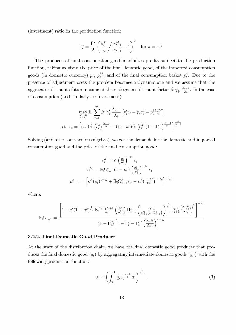
(investment) ratio in the production function:

Γst =Γs

2

µsMtst

ÁsMt−1st−1− 1¶2

for s = c, i

The producer of final consumption good maximizes profits subject to the production

function, taking as given the price of the final domestic good, of the imported consumption

goods (in domestic currency) pt, pMt , and of the final consumption basket pct . Due to the

presence of adjustment costs the problem becomes a dynamic one and we assume that the

aggregator discounts future income at the endogenous discount factor βγLt+1λt+1λt. In the case

of consumption (and similarly for investment):

maxcdt ,c

Mt

Et∞Xτ=0

βτeγLτ λt+τλt

£pctct − ptc

dt − pMt cMt

¤s.t. ct =

h(nc)

1εc

¡cdt¢ εc−1

εc + (1− nc)1εc

¡cMt (1− Γct)

¢ εc−1εc

i εcεc−1

Solving (and after some tedious algebra), we get the demands for the domestic and imported

consumption good and the price of the final consumption good:

cdt = nc³ptpct

´−εcct

cMt = EtΩct+1 (1− nc)

³pMtpct

´−εcct

pct =hnc (pt)

1−εc + EtΩct+1 (1− nc)

¡pMt¢1−εci 1

1−εc

where:

EtΩct+1 =

"1− β (1− nc)

1εc Et

γLt+1λt+1λt

³pctpMt

´Πct+1

µct+1

cMt+1(1−Γct+1)

¶ 1εc

Γc 0t+1(∆cMt+1)

2

∆ct+1

#−εc(1− Γct)

h1− Γct − Γc 0t

³∆cMt∆ct

´i−εc3.2.2. Final Domestic Good Producer

At the start of the distribution chain, we have the final domestic good producer that pro-

duces the final domestic good (yt) by aggregating intermediate domestic goods (yit) with the

following production function:

yt =

µZ 1

0

(yit)ε−1ε di

¶ εε−1

. (3)

13

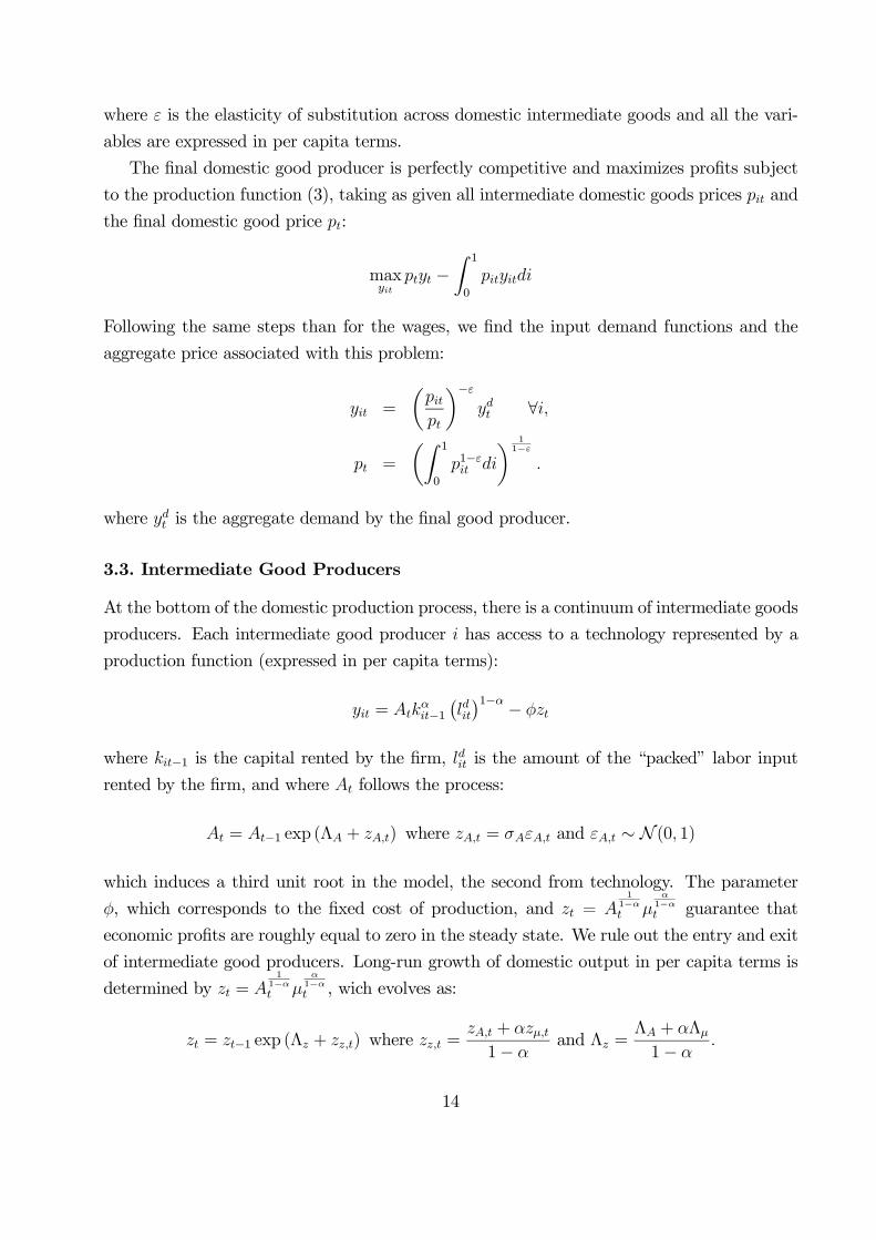
where ε is the elasticity of substitution across domestic intermediate goods and all the vari-

ables are expressed in per capita terms.

The final domestic good producer is perfectly competitive and maximizes profits subject

to the production function (3), taking as given all intermediate domestic goods prices pit and

the final domestic good price pt:

maxyit

ptyt −Z 1

0

pityitdi

Following the same steps than for the wages, we find the input demand functions and the

aggregate price associated with this problem:

yit =

µpitpt

¶−εydt ∀i,

pt =

µZ 1

0

p1−εit di

¶ 11−ε

.

where ydt is the aggregate demand by the final good producer.

3.3. Intermediate Good Producers

At the bottom of the domestic production process, there is a continuum of intermediate goods

producers. Each intermediate good producer i has access to a technology represented by a

production function (expressed in per capita terms):

yit = Atkαit−1

¡ldit¢1−α − φzt

where kit−1 is the capital rented by the firm, ldit is the amount of the “packed” labor input

rented by the firm, and where At follows the process:

At = At−1 exp (ΛA + zA,t) where zA,t = σAεA,t and εA,t ∼ N (0, 1)

which induces a third unit root in the model, the second from technology. The parameter

φ, which corresponds to the fixed cost of production, and zt = A1

1−αt μ

α1−αt guarantee that

economic profits are roughly equal to zero in the steady state. We rule out the entry and exit

of intermediate good producers. Long-run growth of domestic output in per capita terms is

determined by zt = A1

1−αt μ

α1−αt , wich evolves as:

zt = zt−1 exp (Λz + zz,t) where zz,t =zA,t + αzμ,t1− α

and Λz =ΛA + αΛμ

1− α.

14

Intermediate goods producers solve a two-stages problem. In the first stage, taken the

input prices wt and rt as given, firms rent ldit and kit−1 in perfectly competitive factor markets

in order to minimize real cost:

minldit,kit−1

wtldit + rtkit−1

s.to : yit =

(Atk

αit−1

¡ldit¢1−α − φzt if Atk

αit−1

¡ldit¢1−α ≥ φzt

0 otherwise

Assuming an interior solution, the solution is:

ldit : wt = mct (1− α)At

µkit−1ldit

¶α

⇒ ldit = mct (1− α)yitwt

kit−1 : rt = mctαAtkα−1it−1

¡ldit¢1−α ⇒ kit−1 = mctα

yitrt

where mct represents real marginal costs and is the Lagrangian multiplier. Substituting this

solution into the production function and solving we obtain:

mct =

µ1

1− α

¶1−αµ1

α

¶αw1−αt rαtAt

Note that the marginal cost does not depend on i: all firms receive the same technology

shocks and all firms rent inputs at the same price.

In the second stage, intermediate good producers choose the price that maximizes dis-

counted real profits. To do so, they consider that are under the same pricing scheme than

households. In each period, a fraction 1− θp of firms can change their prices. All other firms

can only index their prices by past inflation of the final domestic good price³Πt =

ptpt−1

´.8

Indexation is controlled by the parameter χ ∈ [0, 1], where χ = 0 is no indexation and χ = 1

is total indexation. The problem of the firms is then:

maxpitEt

∞Xτ=0

(βθp)τ eγLτ λt+τλt

(ÃτY

s=1

Πχt+s−1

pitpt+τ

−mct+τ

!yit+τ

)

s.to : yit+τ =

ÃτY

s=1

Πχt+s−1

pitpt+τ

!−εyt+τ

where the marginal value of a dollar to the household, is treated as exogenous by the firm.

Since we have complete markets in securities and the utility function is separable in con-

8There are different possible prices for indexation. Here we pick a simple alternative.

15

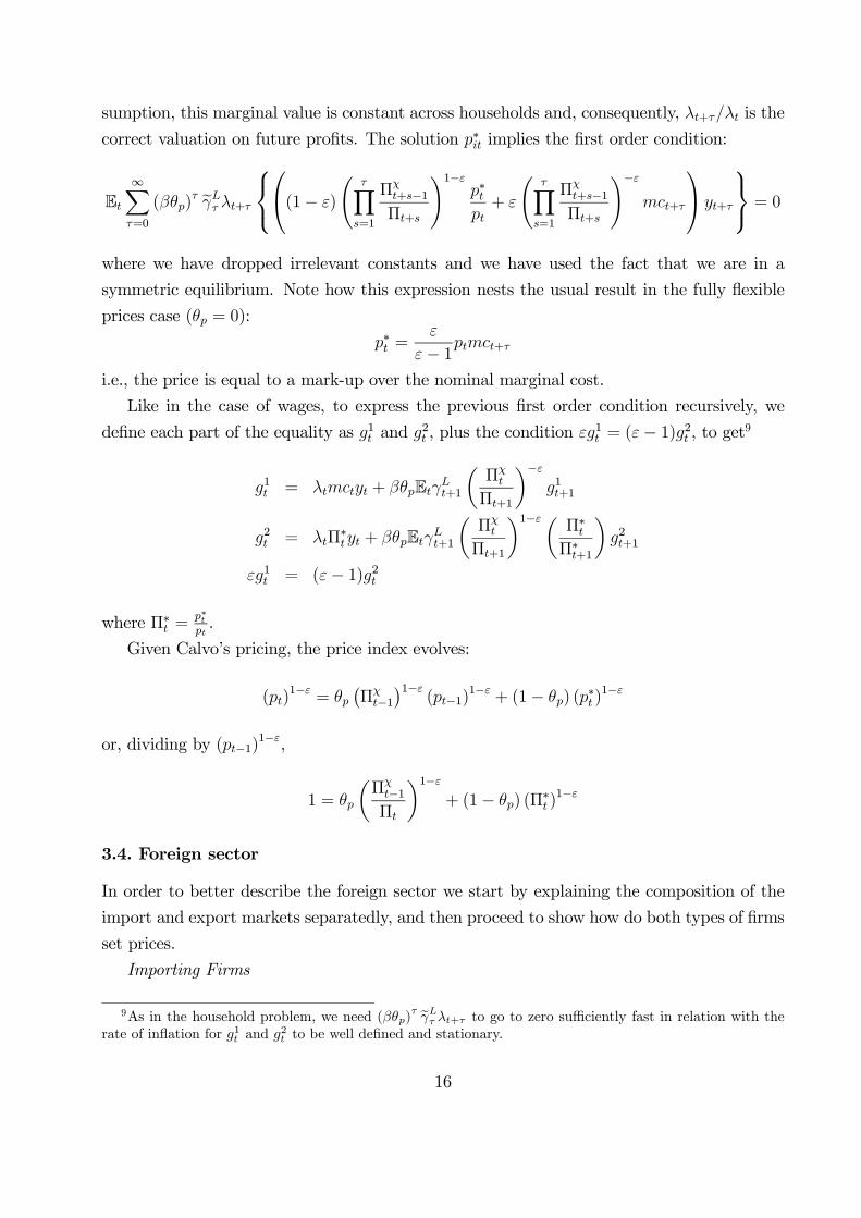
sumption, this marginal value is constant across households and, consequently, λt+τ/λt is the

correct valuation on future profits. The solution p∗it implies the first order condition:

Et∞Xτ=0

(βθp)τ eγLτ λt+τ

⎧⎨⎩⎛⎝(1− ε)

ÃτY

s=1

Πχt+s−1Πt+s

!1−εp∗tpt+ ε

ÃτY

s=1

Πχt+s−1Πt+s

!−εmct+τ

⎞⎠ yt+τ

⎫⎬⎭ = 0

where we have dropped irrelevant constants and we have used the fact that we are in a

symmetric equilibrium. Note how this expression nests the usual result in the fully flexible

prices case (θp = 0):

p∗t =ε

ε− 1ptmct+τ

i.e., the price is equal to a mark-up over the nominal marginal cost.

Like in the case of wages, to express the previous first order condition recursively, we

define each part of the equality as g1t and g2t , plus the condition εg1t = (ε− 1)g2t , to get9

g1t = λtmctyt + βθpEtγLt+1µ

Πχt

Πt+1

¶−εg1t+1

g2t = λtΠ∗tyt + βθpEtγLt+1

µΠχt

Πt+1

¶1−εµΠ∗tΠ∗t+1

¶g2t+1

εg1t = (ε− 1)g2t

where Π∗t =p∗tpt.

Given Calvo’s pricing, the price index evolves:

(pt)1−ε = θp

¡Πχt−1¢1−ε

(pt−1)1−ε + (1− θp) (p

∗t )1−ε

or, dividing by (pt−1)1−ε,

1 = θp

µΠχt−1Πt

¶1−ε+ (1− θp) (Π

∗t )1−ε

3.4. Foreign sector

In order to better describe the foreign sector we start by explaining the composition of the

import and export markets separatedly, and then proceed to show how do both types of firms

set prices.

Importing Firms

9As in the household problem, we need (βθp)τ eγLτ λt+τ to go to zero sufficiently fast in relation with the

rate of inflation for g1t and g2t to be well defined and stationary.

16

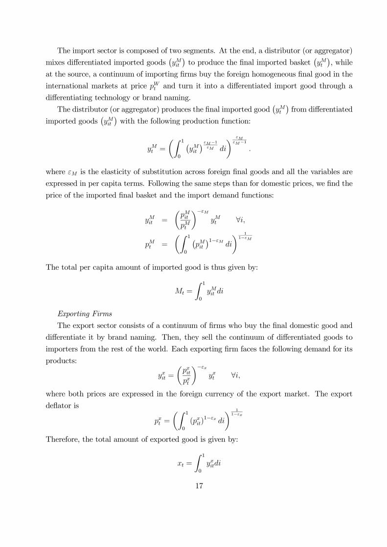
The import sector is composed of two segments. At the end, a distributor (or aggregator)

mixes differentiated imported goods¡yMit¢to produce the final imported basket

¡yMt¢, while

at the source, a continuum of importing firms buy the foreign homogeneous final good in the

international markets at price pWt and turn it into a differentiated import good through a

differentiating technology or brand naming.

The distributor (or aggregator) produces the final imported good¡yMt¢from differentiated

imported goods¡yMit¢with the following production function:

yMt =

µZ 1

0

¡yMit¢ εM−1

εM di

¶ εMεM−1

.

where εM is the elasticity of substitution across foreign final goods and all the variables are

expressed in per capita terms. Following the same steps than for domestic prices, we find the

price of the imported final basket and the import demand functions:

yMit =

µpMitpMt

¶−εMyMt ∀i,

pMt =

µZ 1

0

¡pMit¢1−εM di

¶ 11−εM

The total per capita amount of imported good is thus given by:

Mt =

Z 1

0

yMit di

Exporting Firms

The export sector consists of a continuum of firms who buy the final domestic good and

differentiate it by brand naming. Then, they sell the continuum of differentiated goods to

importers from the rest of the world. Each exporting firm faces the following demand for its

products:

yxit =

µpxitpxt

¶−εxyxt ∀i,

where both prices are expressed in the foreign currency of the export market. The export

deflator is

pxt =

µZ 1

0

(pxit)1−εx di

¶ 11−εx

Therefore, the total amount of exported good is given by:

xt =

Z 1

0

yxitdi

17

Finally, appealing to symmetry and assuming that there is no home bias against our exports

since we represent a negligible part of the world, the world demand of our exports is:

yxt =

µpxtpWt

¶−εWyWt .

Therefore, we have that

yxit =

µpxitpxt

¶−εx µ pxtpWt

¶−εWyWt ∀i.

The evolution of world demand is exogenously given by

yWt =¡yW¢(1−ρyW ) ¡yWt−1¢ρyW e(σyW ε

yW ,t)

and world inflation by:

ΠWt =

¡ΠW

¢(1−ρΠW ) ¡ΠWt−1¢ρ

ΠW e(σΠW εΠW ,t)

Price-setting in the foreign sector:

In order to allow for incomplete exchange rate pass-through to import and export prices

we assume that importing and exporting firms in the foreign sector face price stickiness à

la Calvo. Since the problem faced by both types of firms is similar, we will describe them

together. In particular, in each period, a fraction 1− θM (1− θX) of importing (exporting)

firms can change their prices. All other importing (exporting) firms can only index their

prices by the past inflation of the final imported (foreign) good³ΠMt = pMt

pMt−1

³ΠWt = pWt

pWt−1

´´.

Indexation is controlled by the parameter χM , χX ∈ [0, 1], where χM , χX = 0 is no indexation

and χM , χX = 1 is total indexation.

Since importing (exporting) firms buy the homogeneous foreign (domestic) good at price

pWt (pt) in the world (domestic) market, their real marginal cost, in domestic (foreign) cur-

rency terms, is equal to mcMt = pWt extpMt

(mcxt =pt

extpxt).

The problem of importing (exporting) firm i is then:

maxpfmit

Et∞Xτ=0

(βθfm)τ eγLτ λt+τλt

(ÃτY

s=1

³Πfmt+s−1

´χfm pfmitpfmt+τ

−mcfmt+τ

!yfmit+τ

)

s.to: yfmit+τ =

ÃτY

s=1

³Πfmt+s−1

´χfm pfmitpfmt+τ

!−εfmyfmt+τ for fm =M,x

18

Proceeding like in the case of domestic prices we get:

gM1t =

⎡⎢⎣ λtextpWtpMt

yMt +

βθMEtγLt+1µ(ΠM

t )χM

ΠMt+1

¶−εMgM1t+1

⎤⎥⎦gM2t =

⎡⎣λtΠM∗t yMt + βθMEtγLt+1

áΠMt

¢χMΠMt+1

!1−εM µΠM∗t

ΠM∗t+1

¶gM2t+1

⎤⎦gx1t =

⎡⎢⎣ λtpt

extpxtyxt+

βθxEtγLt+1µ(ΠWt )

χx

Πxt+1

¶−εxgx1t+1

⎤⎥⎦gx2t = λtΠ

x∗t yxt + βθxEtγLt+1

áΠWt

¢χxΠxt+1

!1−εx µΠx∗t

Πx∗t+1

¶gx2t+1

εMgM1t = (εM − 1)gM2

t ; εxgX1t = (εx − 1)gX2

t

where ΠM∗t =

pM∗

t

pMtand Πx∗

t =px∗

t

pxt.

Given Calvo’s pricing, the import and export price indices evolve as:

1 = θM

áΠMt−1¢χM

ΠMt

!1−εM+ (1− θM)

¡ΠM∗t

¢1−εM1 = θx

áΠWt−1¢χx

Πxt

!1−εx+ (1− θx)

¡Πx∗t

¢1−εxEvolution of Net Foreign Assets

To close the foreign sector, we have to determine the evolution of net foreign assets. The

balance of payments, including the risk premium, evolves as follows:Z 1

0

extbWjt dj = RW

t−1Γ³extebWt−1, ξbWt−1´ ext 1γLt

Z 1

0

bWjt−1dj + extpxt y

xt − extp

Wt Mt

where we have use the fact that:Z 1

0

pxityxitdi =

Z 1

0

pxit

µpxitpxt

¶−εxyxt di = (p

xt )

εx yxt

Z 1

0

(pxit)1−εx di = pxt y

xt

19

3.5. The Monetary Authority

Monetary policy is controlled by the European Central Bank (ECB), which sets the nominal

interest rates for the euro area (Rt) according to the Taylor rule:

Rt

R=

µRt−1

R

¶γR

⎛⎝µΠEAt

ΠEA

¶γΠ

⎛⎝ γLEA

tyEAtyEAt−1

exp¡ΛLEA + ΛyEA

¢⎞⎠γy⎞⎠1−γR

exp (ξmt )

through open market operations, where ΠEA represents the Euro Area target level of inflation,

R Euro Area steady state nominal gross return of capital, and Λyd the Euro Area steady state

gross growth rate of yEAt . The term ξmt is a random shock to monetary policy that follows

ξmt = σmεmt where εmt is distributed according to N (0, 1). The presence of the previousperiod interest rate, Rt−1, is justified because we want to match the smooth profile of the

interest rate over time observed in the data. Obviously, the Spanish economy contributes

to Euro Area inflation and output according to its relative size. Note that R is beyond the

control of the monetary authority, since it is equal to the steady state real gross return of

capital plus the target level of inflation.

In practice, it is difficult to solve a DSGE model with such a taylor rule since due the small

weight of Spain in the Euro Area aggregate (10%) the indeterminacy region is very large.

One way to solve this problem is to build a model of a two-country small open monetary

area, like BEMOD. This was not the objective of this work.

Instead, we adopt two alternative approaches depending on the objective of the exercise.

In the first approach we assume the domestic economy has an independent monetary policy

and thus the domestic monetary authority sets the nominal interest rate. This is equivalent to

setting a weight of 1 for Spain’s aggregates in the Taylor rule above. This would correspond

to time before the Euro Area was set up and we use it when estimating the model over the

whole sample period (1986-2007), when doing historical decomposition of shocks or in some

conterfactual exercises. In the second approach, we assume Spain is too small to have a

significant influence on the ECB’s Taylor rule, thus Spain considers the nominal interest rate

to be exogenously set by the ECB and the nominal exchange rate with the rest of the area is

constant. In this case we assume Spain only trades with the rest of the area and ignore the

rest of the world. This is the approach we use when estimating over the most recent period

(1997-2007) or when doing policy analysis related to the current situation.

20

3.6. The Government Problem

The per capita government budget constraint is:

ebt = gtztydt

+Ttydt+

1

γLt ydtΠt

mt−1

pt−1+1

γLtRt−1

R 10bjt−1dj

ptydt

−¡rtujt − μ−1t δ

¢τkkt−1ydt− τwwt

ldtydt− τ c

pctpt

ctydt− mt

pt

1

ydt

where we have redefined the level of outstanding debt as a proportion of nominal output asebt = 10 bjtdj

ptydt.10 The level of real government consumption appears multiplied by zt to keep it

a stationary share of output, which is exogenous and determined according to a stochastic

process:

log gt =¡1− ρg

¢log g + ρg log gt−1 + σgεg,t where εg,t ∼ N (0, 1),

Fiscal policy must be designed to prevent the level of debt to explode. Since all tax rates

are assumed to be constant, we assume that lump-sum taxes as a proportion of output in per

capita terms (Ttyt) respond sufficiently to prevent deviations of the level of debt as a proportion

of GDP (ebt) from target (eb = ³ bpyd

´):

Ttydt= T0 − T1

³ebt −eb´3.7. Aggregation

To close the model we need aggregation conditions for each of the markets considered: goods,

labor, import and export markets.

In the case of goods market, starting from the expression for per capita aggregate

demand of the domestic final good

ydt = cdt + idt + gtzt + μ−1t Φ [ut] kt−1 + xt,

using the equation determining the demand for each intermediate producer’s good (yit =³pitpt

´−εydt ) and the production function (yit = Atk

αit−1

¡ldit¢1−α

), and integrating over all firms

10One can show that the government budget constraint is correct by inserting it into the households budgetconstraint (evaluated at the aggregate level), which implies that all the tax-terms except gt cancel as theyshould.

21

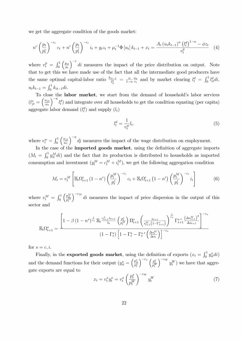
we get the aggregate condition of the goods market:

ncµptpct

¶−εcct + ni

µptpit

¶−εiit + gtzt + μ−1t Φ [ut] kt−1 + xt =

At (utkt−1)α ¡ldt ¢1−α − φzt

vpt(4)

where vpt =R 10

³pitpt

´−εdi measures the impact of the price distribution on output. Note

that to get this we have made use of the fact that all the intermediate good producers have

the same optimal capital-labor ratio kit−1ldit

= α1−α

wtrtand by market clearing ldt =

R 10lditdi,

utkt−1 =R 10kit−1di.

To close the labor market, we start from the demand of household’s labor services

(lsjt =³wjtwt

´−ηldt ) and integrate over all households to get the condition equating (per capita)

aggregate labor demand (ldt ) and supply (lt)

ldt =1

vwtlt. (5)

where vwt =R 10

³wjtwt

´−ηdj measures the impact of the wage distribution on employment.

In the case of the imported goods market, using the definition of aggregate imports(Mt =

R 10yMit di) and the fact that its production is distributed to households as imported

consumption and investment (yMt = cMt + iMt ), we get the following aggregation condition

Mt = vMt

"EtΩc

t+1 (1− nc)

µpMtpct

¶−εcct + EtΩi

t+1

¡1− ni

¢µpMtpit

¶−εiit

#(6)

where vMt =R 10

³pMitpMt

´−εMdi measures the impact of price dispersion in the output of this

sector and

EtΩst+1 =

"1− β (1− ns)

1εs Et

γLt+1λt+1λt

³pstpMt

´Πst+1

µst+1

sMt+1(1−Γst+1)

¶ 1εs

Γs 0t+1(∆sMt+1)

2

∆st+1

#−εs(1− Γst)

h1− Γst − Γs 0t

³∆sMt∆st

´i−εsfor s = c, i.

Finally, in the exported goods market, using the definition of exports (xt =R 10yxitdi)

and the demand functions for their output (yxit =³pxitpxt

´−εx ³ pxtpWt

´−εWyWt ) we have that aggre-

gate exports are equal to

xt = vxt yxt = vxt

µpxtpWt

¶−εWyWt (7)

22

where vxt =R 10

³pxitpxt

´−εxdi.

Finally, by the properties of price indices under Calvo’s pricing mechanism, price disper-

sions evolve according to:

vpt = θp

µΠχt−1Πt

¶−εvpt−1 + (1− θp)

¡Π∗t

¢−εvwt = θw

µwt−1

wt

Πχwt−1Πt

¶−ηvwt−1 + (1− θw) (Π

∗wt )

−η

vMt = θM

áΠMt−1¢χM

ΠMt

!−εMvMt−1 + (1− θM)

¡ΠM∗t

¢−εMvxt = θx

áΠWt−1¢χx

Πxt

!−εxvxt−1 + (1− θx)

¡Πx∗t

¢−εx. (8)

4. Equilibrium and model solution

A definition of equilibrium in this economy is standard. However, since there is growth in

the model induced by technological change, most of the variables are growing on average.11

Before we can solve the model, we need to redefine all the relevant variables to obtain a

system of stationary variables. Hence, we define ect = ctzt, eλt = λtzt, ert = rtμt, eqt = qtμt,ext = xt

zt, ewt =

wtzt, ew∗t = w∗t

zt, ekt = kt

ztμt, emt =

mt

zt, eydt = ydt

ztand the growth rates ezt = zt

zt−1,eAt =

At

At−1, eμt = μt

μt−1, eLt =

LtLt−1

. In addition, we express all the relative prices in terms of the

five relevant ones (pct

pt, pitpt, pMt

pt, extpxt

ptand extpWt

pt). Then, to solve the model we find the steady

state and we can loglinearize the equilibrium conditions around it. The full set of non-linear

and log-linearized equilibrium conditions are included in the appendix.

4.1. The Steady-State

Now, we will find the deterministic steady-state of the model. First, since in the steady-

state the law of one price must hold,³ex pW

p

´= 1. Second, the exchange rate is assumed

to be constant (∆ex = 1), which means that the domestic nominal interest rate is equal

to the world nominal interest rate (R = RW = Πzβ), and the net foreign asset position

is assumed to be equal to zero (expressed in domestic currency), so that nominal exports

equal nominal imports (ex³ex px

p

´= vx

³ex pW

p

´ fM). Third, let ez = exp (Λz), eμ = exp (Λμ),eA = exp (ΛA) and γL = exp (ΛL) Also, given the definition of ec, ext, ewt, ew∗t , and eydt , we have11Population growth does not affect the equilibrium since the variables are already expressed in per capita

terms.

23

that Λc = Λi = Λw = Λw∗ = Λyd = Λz, and u = d = ϕ = 1 and g = g.

In addition, we need to choose functional forms for all the adjustment cost functions in the

model: Φ [·], S [·], Γs [·] and Γ³eb∗´. For Φ [u] we pick: Φ [ut] = Φ1 (ut − 1)+ Φ2

2(ut−1)2. Since

in the steady state we have u = 1, then Φ [1] = 0 and Φ0 [1] = Φ1. The investment adjustment

cost function is ShγLt

itit−1ezti = S

hit

it−1

i= κ

2(γLt

itit−1ezt−Λi)

2. Then, along the balanced growth

path, S£γLez¤ = S [Λi] = S0 [Λi] = 0. Finally, the imports adjustment cost function along the

balanced growth path is Γs = Γs

2

³sM

s

.sM

s− 1´2, thus Γs = Γs 0 = 0. With respect to the

adjustment cost of risk premium, we assume Γ³exteb∗t , ξb∗t ´ = e(−Γ

b∗(extb∗t−exb∗)+ξb∗t ). Since in

the steady state the domestic and world interest rates are the same, R = R∗Γ³exeb∗, 0´, we

have Γ³exeb∗, 0´ = e0 = 1 and Γ0

³exeb∗´ = −Γb∗e0 = −Γb∗.

Therefore, using these results and the equilibrium conditions we can simplify the steady-

state to the following set of equations determining ld, and the rest of variables are recursive

to these: ek = µ α

1− α

ewer ezeμ¶ld = Ωld.

eyd = Azekα ¡ld¢1−α − φ

vp

ei = µγL − (1− δ)eμez¶ek

ec = 1

nc

µpc

p

¶−εc ⎡⎣eyd − niµpi

p

¶εiei− vx

³ex pW

p

´³ex px

p

´ fM − g

⎤⎦

fM = vM

⎡⎢⎣(1− nc)

⎡⎣³pM

p

´³pc

p

´⎤⎦−εc ec+ ¡1− ni

¢⎡⎣³pM

p

´³pi

p

´⎤⎦−εiei

⎤⎥⎦eλ = µez − hβγLez − h

¶1ec (1 + τ c)

pc

p

1− βθwezη(1+ϑ)Πη(1−χw)(1+ϑ)γL

1− βθwezη−1Π−(1−χw)(1−η)γL =ψ¡w∗

w

¢−ηϑ ¡ld¢ϑ

η−1η(1− τw) ew∗eλ

24

Or alternatively, solving we have the following equation on ld:

1− βθwezη(1+ϑ)Πη(1−χw)(1+ϑ)γL

1− βθwezη−1Π−(1−χw)(1−η)γL =ψ¡w∗

w

¢−ηϑ ¡ld¢ϑ

η−1η(1− τw) ew∗

µ ez − hez − hβγL

¶∗

∗

⎧⎨⎩(1 + τ c)

Λc

µpc

p

¶1−εc ⎡⎣ hAzΩα (vp)−1 − Λi³pi

p

´εi ³γL−(1−δ)μz

´Ωild

−φ (vp)−1 − g

⎤⎦⎫⎬⎭Note that this is a nonlinear equation. Therefore we will use a root finder to find ld. Whereew∗, ew,³pc

p

´,³pi

p

´and vp are only functions of parameters, while Π,ΠM are parameters to be

estimated and ΠW , eyW are exogenously given.

5. Estimating the model

We will confront our model with the data using Bayesian methods. The Bayesian paradigm is

a powerful and flexible perspective for the estimation of DSGE models (see the survey by An

and Schorfheide, 2006). First, Bayesian analysis is a coherent approach to inference based on

a clear set of axioms. Second, the Bayesian approach handles in a natural way misspecification

and lack of identification, both serious concerns in the estimation of DSGE models (Canova

and Sala, 2006). Moreover, it has desirable small sample and asymptotic properties, even

when evaluated by classical criteria (Fernández-Villaverde and Rubio-Ramírez, 2004). Third,

the use of priors is a flexible procedure to introduce presample information that the researcher

may have and to reduce the dimensionality problem associated with number of parameters.

Formally, let p(Ψ|m) denote the prior distribution of the vector Ψ ∈ with structural

parameters for some model m ∈ M , and let p(Y T |Ψ,m) denote the likelihood function forthe observed data, Y T = y1, ..., yT, conditional on parameter vector Ψ and model m.

The joint posterior distribution of the parameter vector Ψ for model m is then obtained

by combining the likelihood function for Y T and the prior distribution of Ψ,

p(Ψφ|Y T ,m) ∝ p(Y T |Ψ,m)p(Ψ|m),

where “∝” indicates proportionality.The Bayesian approach combines the likelihood of the model L

¡Y T ;Ψ

¢with a prior

density for the parameters p(Ψ) to form a posterior:

p(Ψ/Y T ) ∝ L¡Y T ;Ψ

¢p(Ψ)

The posterior summarizes the uncertainty regarding the parameters, and it can be used for

25

point estimation. For example, under a quadratic loss function, our point estimates will be

the mean of the posterior.

Since the posterior is also difficult to characterize, we generate draws from it using a

Metropolis-Hastings algorithm. We use the resulting empirical distribution to obtain point

estimates, standard deviations, etc.

5.1. Data

In estimating MEDEA, we use time series for 9 variables (see Figure ??): real GDP³yd,Ot

´,

real private consumption¡cOt¢, total employment in hours

³ld,Ot

´, real compensation per

hour (total compensation/total hours/GDP deflator)¡wOt

¢, consumption deflator inflation³

Πc,Ot

´, total population over 16 years of age

¡LOt

¢, Euro area nominal interest rate

¡ROt

¢,

inflation of Spanish competitors prices³ΠW,Ot

´, Spain’s foreign demand

³yW,Ot

´. All the

time series are taken from National Accounts published by INE, except for the foreign sector

variables and the nominal interest rate which come from the database developed for the REMS

model (BDREMS)12. The sample period ranges from 1986q1-2007Q413. We have excluded

investment from the estimation since it has grown in the last decade at an unprecedented

pace, mainly due to the construction sector, which we believe would be difficult to explain

using a model without a housing and financial frictions.

Empirical variables Since the model incorporates growth, we do not need to transform

the variables for estimation. Instead, in order to take the model to the data, we have to take

into account the fact that the variables observed in the economy are different from the ones

in the model. First, in the log-linearized version of the model all variables are expressed as

log deviations with respect to their steady state value. Second, all variables in the model

are expressed in per-capita terms dividing by the population (Lt). Third, some real variables

in the model are made stationary by dividing by zt. Therefore, we need to add equations

stating the relationship between empirical and model variables. In the case of real per capita

variables, like real GDP per capita, the growth rate of the empirical variable³yd,Ot

´is equal

to the growth rate of the model variable (in per capita terms)¡ydt¢(do not confuse with

the transformed stationary variable eydt = ydtzt) plus population growth (γLt ). However, since

we estimate the stationary log-linearized version of the model, we need to re-express this

definition in terms of stationary variables expressed as log-linear deviations from steady state

12The BDREMS database is available in the following webpage:http://www.sgpg.pap.meh.es/SGPG/Cln_Principal/Presupuestos/Documentacion/BasedatosmodeloREMS.htm13The deep changes in the structure of the Spanish economy stops us from using data prior to 1986.

26

(beyt = log ytzt− log y

z). Finally, we have to remember that in the stationary model we have the

growth rate of technology in log-linear deviations from steady state (bezt = log ztzt−1− log ez).

Overall, the transition equation for output is as follows

4 log yd,Ot = ∆ log yt + γLt = ∆beyt + bezt + bγLt + log ez + γL

An exception is employment in hours, since it is stationary in per capita terms in the model,

we only have to add population growth

4 log ld,Ot = ∆ log ldt + γLt = ∆ logbeyt + bγLt + γL

In the case of nominal variables, like inflation and interest rates, we only have to add the

steady state value to the model variable:

logΠc,Ot = bΠc

t + logΠc

logROt = bRt + logR

Figure 1 compares shows the original and transformed variables for the sample period.

5.2. Calibration and prior distributions

5.2.1. Calibration

The model has 59 parameters, of which 12 are calibrated and the remaining 47 estimated.

The calibration is shown in table 1. Several theoretical and empirical reasons explain why one

may not want to estimate all the parameters of the model. First, some parameters are difficult

to identify with the model structure, like the discount factor β. This parameter is set to be

consistent with an annualised nominal interest rate of 2.5% and an inflation objective of 2%.,

which is set so that the steady state annual nominal interest rate (R = RW = Πzβ) is 4.5%.

Second, other parameters like the depreciation rate δ or the labor share α, are estimated

better using micro data, while other would require adding more data series to the estimation,

like the three tax rates (τ c, τw, τk). Third, there are parameters which are irrelevant for the

model solution, like the coefficient of money demand in the utility function, υ. Finally, the

parameters of the Taylor rule are set equal to the standard estimation results for the Euro

Area. The two fiscal parameters have not yet been included in the estimation and thus are

set to their empirical values.

27

Table 1: Calibrated parameters

value reason value reason

β 0.99 not identified γy 0.125 R.Taylor UE

υ 0.1 irrelevant τ c 0.113 data on taxes

δ 0.0175 micro data τw 0.341 data on taxes

α 0.3621 micro data τk 0.219 data on taxes

γR 0.8 R.Taylor UE g 0.17 —

γΠ 1.7 R.Taylor UE b 0.40 —

5.2.2. Prior distributions:

The first vertical panel in Table 2 summarizes our assumptions regarding prior distributions

for the estimated parameters. Our approach has been to set priors as loose as possible.

Thus, we have chosen Uniform distributions for the priors with a range covering all the

theoretically feasible values for each parameter. In this way, we have set a range of (0, 1),for

the labour supply coefficient, price and wage Calvo and indexation parameters, adjustment

costs parameters, autorregressive coefficients (except the labour supply shock in which we

have chosen (0, 0.9)) and the standard deviations of shocks. In the case of the elasticity of

substitution parameters we have set a range of (6, 10). In a few cases, we have decided to

impose stronger priors, by assuming beta distributions. In particular, the habits coefficient

and the home bias coefficients, because the data wanted to take them to unrealistic parameter

values. Finally, we also set beta distributions for the parameters determining growth in the

model, since it helps to identify them.

5.3. Estimation results

The choice of the sample period over which to estimate the structural parameters is a compli-

cated issue in the Spanish case. There have been significant changes in the Spanish economy

since the mid-nineties. The most important of which was the set up of the euro area, but also

relevant have been the rise in labor force participation, mainly by women, and in inmigration.

Some papers in the literature have thus decided to only use the period since the euro area was

conceived, that is from 1997 onwards to avoid having to deal with structural breaks in the

sample and with the change in the implementation of monetary policy. The drawback is that

the sample becomes fairly small and the estimation will require tighter priors. In addition,

it is not sure that the structural break will not be a problem since the impact of the creation

of the monetary union probably lasted for several years after 1997. Not to forget that the

other changes in the structure of the Spanish economy mentioned above may also have had

28

important effects.

Instead, in this paper we have decide to proceed in two stages. First, we use data for

the full sample 1986-2007, assuming that Spain had an independent monetary policy during

this period. This allows us to set fairly loose priors and let the data speak up as much as

possible. We had to drop the data before 1986 because the changes in the structure of the

Spanish economy in the early eighties were too substantial. Then, we check the stability of

the point estimates by estimating the model separatedly for two subsamples, but maintaining

the assumption of an independent monetary authority: one for the period before the euro area

was set up (1986-1996) and the other from 1997 onwards. Finally, we estimate the model over

the most recent subsample assuming Spain is too small to have any influence on the ECB‘s

decisions to set interest rates, that is, the interest rate is exogenous and the exchange rate is

constant.

The right-hand panel of Table 2 present the estimation results for the full sample (1986Q1-

2007Q4), while the ones in Table 3 present the results for the two subsamples considered

(1986Q1-1996Q4 and 1997Q1-2007Q4) as well as the model with no independent monetary

policy. The entries in the posterior mode column refer to the values of the structural parame-

ters that are obtained by maximising the model’s posterior distribution. The remaining four

columns report the median, standard deviation, the 5th and 95th percentiles of the poste-

rior distribution. All of them are computed using a Metropolis-Hasting algorithm in dynare,

based on a Markov chain with 5 million draws, with 2.5 million draws being discarded as

burn-in draws.

5.3.1. Estimation results using the full sample

First, Figure X showing the draws of the posterior sampling algorithm (to be included) shows

that it has converged for all the estimated parameters, since in all cases the algorithm has

stabilized after x number of draws. 14 Second, Figure 2 shows the smoothed estimates of the

innovation component of structural shocks. All of them are clearly stationary. However, it is

worth noting that the variance of the shocks seems to have fallen in the second part of the

sample, except in the case of the population growth shock, that has increased, in line with

the rise in population growth in Spain over the last decade.

Third, Figures 3-7 compare the prior and posterior distributions of each parameter. Since

we have used uniform distributions for the priors of most parameters, the posterior distrib-

utions are not as well behaved as when other distributions are chosen. Exceptions are the

14We will also provide the other diagnostic checks included in dynare for the final version of the paper. Sofar we are only using one chain of 5 million draws, but dynare only provides these tests for several chains.

29

indexation of import prices, the coefficient of the fiscal rule, the adjustment cost parameter of

the risk premium and imported investment and the autorregressive parameter of the foreign

demand shock, in which we seem to find signs of a twin-peaked posterior distribution (need

to check that in these cases the algorithm has correctly converged). Although for most of

these cases both peaks of the distribution imply fairly similar estimates, which would not

change the properties of the model, more work needs to be done to check their robustness.

Nevertheless, in almost all cases, the observed data is very informative about the posterior

distribution of the parameters. Exceptions are the steady state growth rate of technology

and population, where the data is completely uninformative, since the prior and the poste-

rior are on top of each other. Therefore, we have set fairly tight priors centered around the

sample mean of observed population growth and observed growth of output per capita, which

according to the model is equal to technological growth. Given this result, one should be

cautious when making inferences about the relative importance in the observed data of each

type of technological growth (neutral and investment specific) included in the model.

A number of estimation results are worth noting. First, the estimate of the utility para-

meters are quite standard. The data strongly support a high estimate of habit persistence,

which is not surprising given the persistence of observed consumption. The estimates of the

production side show that the fixed costs of production are very close to zero.

Second, the estimated elasticities of substitution between different types of intermediate

goods produced are relatively similar, implying a mark-up between 13.5% in the case of

domestic goods and 12% in the case of export goods, while the wage mark-up is somewhat

higher, at around 15%. This is not surprising given the rigidities of the Spanish labour

market, where wages are mainly set by insiders with long-term contracts and thus high

bargaining power. With respect to the demand elasticity of substitution between imported

and domestically produced goods the estimates are also similar. In contrast, the adjustment

cost parameters associated with changing the import content of varies substantially across

both types of goods, being much higher for investment. Moreover, the data is very informative

about this.

Third, on the nominal side, we find important differences across sectors of the economy.

The estimate of the calvo parameter is very high for intermediate domestic goods, although

not different from values generally obtained for the euro area (Smets and Wouters (2003)),

but quite low for the import and export intermediate goods, and the same is true for wages. In

contrast, indexation is very close to one for wages,which seems the direct consequence of the

(ex-ante) indexation mechanism inherent in Spanish wage aggreements. However, indexation

is inexistent in prices of domestically produced goods, while indexation is a bit higher in the

import and export sectors. Moreover, these differences across sectors of production and the

30

labour market are strongly supported in the data.

Fourth, the estimates for the home bias in consumption and investment are rather puz-

zling. Although input-output tables indicate that in Spain there is a larger home bias in

consumption than investment (70% versus 50%), this difference is no way near the estima-

tion results. However, the data is very informative about these point estimates, since imposing

beta priors has not changed the results. A posible explanation may be that we are not using

investment data in the estimation, but more work also needs to be done to understand this

issue.

Finally, the point estimates for the autorregressive parameters of shocks processes show

that domestic shocks are very persistent, specially the domestic demand ones, public con-

sumption and preferences. This suggests that the model has difficulty generating the persis-

tence present in the demand data and thus it resources to making these shocks very persistent.

This could also reflect the impact of a structural break in the data. However, as was men-

tioned above, the sample is still too short to test with standard econometric techniques. The

foreign demand and inflation shocks have much lower persistence.

5.3.2. Stability of estimation results across the two subsamples.

Comparing the results across the two subsamples (see Table 3) the point estimates are rather

similar for most structural parameters, suggesting that there is no clear structural break in

the data for this period. The exception are the standard deviation of shocks, which have

all fallen markedly, except for the population shock, which has increased. This was already

noticeable in the graph of the innovations for the whole sample period, as was mentioned

above. In addition, the estimate of the adjustment cost of the import content of consumption

goods is smaller in the most recent sample, while the one on investment is slightly higher.

Finally, the Calvo parameter on imported intermediate goods is a bit lower, while the one on

wages has almost doubled.

5.3.3. Estimation results without independent monetary policy.

The results of estimating the model with an exogenous nominal interest rate and a constant

nominal exchange rate are reported in the third panel of Table 3. (To be completed).

6. Model properties.

In this section we describe the steady state properties of the estimated model and its impulse

response functions. (To be completed).

31

Table 4 shows that the steady state ratios implied by the point estimates, discussed above,

are comparable with the ones observed in the data.

Figures 8-13 show the impulse response functions of some transitory shocks, as well as

the 5% and 95% confidence bands. Since there is growth in the model due to technological

progress and increase in the population, the real variables in the model are expressed in per

capita efficiency units. In some cases, mainly supply-side shocks, the behaviour of variables

defined in this way may seem confusing. Thus, in the simulations we show instead the growth

rates of real variables expressed in the same units as in the data. That is, for example gyobs

is equal to total real GDP growth.

In all cases we show a one standard deviation shock to the corresponding innovation. The

simulation results are very standard.

7. Applications.

7.1. Historical decomposition

MEDEA can be used to ilustrate what have been the driving forces behind the Spanish eco-

nomic growth during the last three decades, by decomposing the observed GDP growth into

the contributions of the structural shocks (see Figures ??-??). To facilitate the presentationwe group the shocks into five categories: technology shocks, labour shocks, demand shocks,

fiscal and monetary policy shocks and foreign shocks.

Looking at the whole period, the main contributors to growth are the labour supply

(mainly population) and demand shocks, explaining each around 40% (1.3 p.p.) of real GDP

growth, while productivity is the third factor in importance explaining over 15% (0.5 p.p.).

The remaining shocks explain little over the long run as one would expect from a neoclassical

growth model. However, things have been different over time. We will divide the analysis

into the three relevant periods: expansion in the late 1980s, the crisis of 1993-95 and the

boom since then until 2007.

The boom of the late eighties was characterized by large productivity growth, but also by

labour supply (mainly population) and positive demand shocks, explaining each about one

third of the real GDP increase, while fiscal policy explained around 5%. Monetary policy

and foreign shocks contributed negatively, limiting GDP growth by around 0.15 and 0.2 p.p.

on average, respectively.

The crisis of the early nineties was characterized by a very strong negative labour supply

shock, mainly due to the large reduction in labour participation that limited growth by

almost 1.9p.p. over this period, and which did not become positive again until 1998. Not

surprisingly, this shock was accompanied by a fairly large negative demand shock, lasting

32

from the end of 1991 until mid 1993, limiting GDP growth by around 1p.p.

In contrast, the long period of continuous real GDP growth experienced since the mid-

nineties was mainly explained by favourable labour supply shocks and demand shocks, while

technology shocks limited growth until 2001, after this moment its contribution has been

positive but very small. In addition, monetary policy shocks and foreign shocks have had

a positive but much smaller contribution. Figure ?? decomposes the contribution of laboursupply shocks into two, labour participation (its a shock to the preferences between work

and leisure, thus a positive contribution means that households are willing to work more

hours per day) and population growth (which means that there are new households in the

economy). The figure suggests that both types of labour supply shocks have been very

important, contributing on average 1.9 percentage points, which represents over 50% of GDP

growth since 1995, reaching in the early 2000s 3.5 p.p., with population growth explaining

on its own over 40% of growth, while labour participation around 10%.

7.2. Counterfactual scenarios.

In this section we analyse several permanent shocks and conterfactual scenarios.

Permanent shocks:

We start by studing the effect of unexpectedly reducing the consumption tax rate by 1%.

First, as shown in Table 5, in the long run this reduction in taxes will have a positive effect

on the Spanish economy, by increasing output per capita in efficient units and hours worked.

Higher labour input pushes up the marginal productivity of capital and increases investment.

On the demand side, the increase in the retribution of capital and the rise real compensation

per worker (the rise in hours compensates the fall in real wages) increase household’s income

and consumption. In order to equilibrate demand and supply, the terms of trade (px/pM) fall

to improve the external position. Figures 17 and 18 draw the transitional dynamics of the

unexpected reduction in consumption taxes (to make the comparison easier, in the charts all

variables are expressed as differences with respect to the initial steady state). Most variable

move fairly to the new steady state. Thus, we see consumption and investment rise thanks

to the increase in total labour compensation and the rental rate of capital, while net exports

expands due to the fall in the terms of trade.

Alternative scenarios:

The historical decomposition of GDP growth showed that population growth has been one

of the important determinants of economic growth during the recent expansion, explaining

around 1.4 pp. of GDP growth (see Table 6). However, this contribution has not been

constant over time. Instead, Figure 19 shows that there has been an important change in the

long-run population growth rate during the sample, increasing from 0.28% on average over

33

the period 1986-96 to 0.35% since then. Therefore, an interesting question is what would

have been GDP growth had this rise in population growth not taken place. This can be

answered with this model. In particular, we would like to see what would have happened

if population growth followed the alternative scenario depicted in Figure 19 (discontinuous

line). That is, we assume that population growth followed a similar path to the historical

one, but shifted downwards, so that the long run mean is equal to the one of the first part

of the sample. Figure 20 and Table 6 show the impact of this alternative scenario. We find

that had population grown at this alternative slower pace, GDP growth would have been

by 0.5pp. lower. That is, the population growth shock experienced in Spain in the current

decade added half a percentage point to economic growth.

8. Conclusions

(To be completed)

34

References

[1] Adolfson, M., S. Laséen, J. Lindé, and M. Villani (2005). “Bayesian Estimation of an

Open Economy DSGEModel with Incomplete Pass-Through.” Sveriges Riksbank Work-

ing Paper Series 179.

[2] An, S. and F. Schorfheide (2006). “Bayesian Analysis of DSGE Models.” Econometric

Reviews, forthcoming.

[3] Andrés, J., P. Burriel, and A. Estrada (2006). “BEMOD: a DSGE Model for the Spanish

Economy and the Rest of the Euro Area.” Documento de Trabajo del Banco de España

0631.

[4] Boscá, J.E., A. Bustos, A. Díaz, R. Doménech, J. Ferri, E. Pérez and L. Puch (2007).

"A Rational Expectations Model for Simulation and Policy Evaluation of the Spanish

Economy." Documento de Trabajo de la Dirección General de Presupuestos D-2007-04.

[5] Boscá, J.E., A. Díaz, R. Doménech, E. Pérez and L. Puch (2008). "The REMSDBMacro-

economic Database of The Spanish Economy." Documento de Trabajo de la Dirección

General de Presupuestos D-2007-04.

[6] Browning, M., L.P. Hansen, and J.J. Heckman (1999). “Micro Data and General Equi-

librium Models.” in J.B. Taylor & M. Woodford (eds.), Handbook of Macroeconomics,

volume 1, chapter 8, 543-633. Elsevier.

[7] Canova, F. and L. Sala (2006). “Back to Square One: Identification Issues in DSGE

Models.” Mimeo, CREI.

[8] Chari, V.V., P. Kehoe and E.R. McGrattan. (2007). "Business Cycle Accounting" Econo-

metrica, 75, 781-836.

[9] Christiano, L., M. Eichenbaum, and C.L. Evans (2005). “Nominal Rigidities and the

Dynamic Effects of a Shock to Monetary Policy.” Journal of Political Economy 113,

1-45.

[10] Christoffel, K., G. Coenen and A. Warne, (2007) “The New Area-Wide Model of the

Euro Area: Specification, Estimation Results and Properties”, mimeo, European Central

Bank.

[11] Christoffel, K., G. Coenen and A. Warne, (2007) “Conditional versus Unconditional

Forecasting with the NewArea-WideModel of the Euro Area”, mimeo, European Central

Bank.

35

[12] Edge, R., M. T. Kiley and J.P. Laforte (2006). "A Comparison of Forecast Performance

Between Federal Reserve Staff Forecasts, Simple Reduced-Form Models, and a DSGE

Model." mimeo, Federal Reserve Board.

[13] Erceg, C., D. Henderson, and A. Levin (2000). “Optimal Monetary Policy with Staggered

Wage and Price Contracts.” Journal of Monetary Economics 46, 281—313.

[14] Erceg, C.J., L. Guerrieri, and Christopher Gust (2006). “SIGMA: A New Open Economy

Model for Policy Analysis.” International Journal of Central Banking 2, 1-50.

[15] Fernández-Villaverde, J. and J. Rubio-Ramírez (2004). “Comparing Dynamic Equilib-

rium Models to Data: a Bayesian Approach.” Journal of Econometrics, 123, 153-187.

[16] Fernández-Villaverde, J. and J. Rubio-Ramírez (2005). “Estimating Dynamic Equilib-

rium Economies: Linear versus Nonlinear Likelihood.” Journal of Applied Econometrics,

20, 891-910.

[17] Fernández-Villaverde, J. and J. Rubio-Ramírez (2007). “Estimating Macroeconomic

Models: A Likelihood Approach.” Review of Economic Studies, forthcoming.

[18] Fernández-Villaverde, J., J. Rubio-Ramírez, and M.S. Santos (2006). “Convergence

Properties of the Likelihood of Computed Dynamic Models.” Econometrica 74, 93-119.

[19] Greenwood, J, Z. Herkowitz, and P. Krusell (1997). “Long-Run Implications of

Investment-Specific Technological Change.” American Economic Review 87, 342-362.

[20] Greenwood, J, Z. Herkowitz, and P. Krusell (2000). “The Role of Investment-Specific

Technological Change in the Business Cycle.” European Economic Review 44, 91-115.

[21] Hall, R. (1997). "Macroeconomic Fluctuations and the Allocation of Time." Journal of

Labor Economics, 15 (1), 223-250.

[22] Harrison, R., K. Nikolov, M. Quinn, G. Ramsey, A. Scott, and R. Thomas (2005). The

Bank of England Quarterly Model. The Bank of England.

[23] Iskrev, N. (2007): “How much do we learn from the estimation of DSGE models? A

case study of identi´rcation issues in a New Keynesian business cycle model,” mimeo,

University of Michigan.

[24] Kai C., G. Coenen and A. Warne (2007). “Conditional and Unconditional Forecasting

with the New Area-Wide Model of the Euro Area.” Mimeo, European Central Bank.

36

[25] Kilponen, J. and Antti Ripatti (2006). “Introduction to AINO.” Mimeo, Bank of Find-

land.

[26] King, R., C. Plosser and Sergio Rebelo (1988). “Production, Growth and Business Cycles

I: The basic neo-classical model" Journal of Monetary Economics 2, 195-232.

[27] Kortelainen, Mika (2002). “EDGE: a Model of the Euro Area with Applications to

Monetary Policy.”, Bank of Finland Studies E:23.

[28] Murchison, S. and A. Rennison (2006). “ToTEM: The Bank of Canada’s New Quarterly

Projection Model.” Bank of Canada Technical Report 97.

[29] Primiceri, G.E., E. Schaumburg and A. Tambalotti (2006). "Intertemporal disturbances.

Mimeo", New York Fed.

[30] Schmitt-Grohé, S. andM. Uribe (2003). “Closing Small Open EconomyModels.” Journal

of International Economics 61, 163-185.

[31] Sims, C.A. (2007). "??" (en página 4 del documento)

[32] Smets, F. and R. Wouters (2003). “An Estimated Stochastic Dynamic General Equi-

librium Model of the Euro Area.” Journal of the European Economic Association, 1,

1123-1175.

[33] Woodford, M. (2003). Interest and Prices: Foundations of a Theory of Monetary Policy,

Princeton University Press.

37

9. Appendix: Equilibrium conditions:

The full set of equilibrium conditions are:

• The first order conditions of the household:

dt

µect − hect−1ezt

¶−1− hEtβγLt+1dt+1 (ect+1ezt+1 − hect)−1 = eλt (1 + τ c)

µpctpt

¶(1)

eλt = Etβeλt+1ezt+1 Rt

Πt+1 (2)

eλt = Et⎧⎨⎩β

eλt+1ezt+1 RWt Γ

³extebWt , ξb

W

t

´Πt+1

ext+1ext

⎫⎬⎭ (3)

ert = Φ0 [ut]

(1− τk)(4)

eqtEtγLt+1 = βEtγLt+1

( eλt+1eλtezt+1eμt+1Ã(1− δ) eqt+1 + ert+1ut+1 (1− τk)

+δτk − Φ [ut+1]

!)(5)

µpitpt

¶= eqtÃ1− S

"γLt

eiteit−1ezt#− S0

"γLt

eiteit−1ezt#γLt

eiteit−1ezt!

+Etβeqt+1 eλt+1eλtezt+1S0"γLt+1

eit+1eit ezt+1#Ã

γLt+1eit+1eit ezt+1

!2(6)

µ emt

pt

¶= dtυ

"βEt

eλt+1ezt+1 Rt − 1Πt+1

#−1(7)

ft =η − 1η

(1− τw) ( ew∗t )1−η eλt (ewt)η ldt + βθwEtγLt+1

µΠχwt

Πt+1

¶1−η µ ew∗t+1ew∗t ezt+1¶η−1

ft+1

(8)

ft = dtϕtψ

µ ew∗tewt

¶−η(1+ϑ) ¡ldt¢1+ϑ

+ βθwEtγLt+1µΠχwt

Πt+1

¶−η(1+ϑ)µ ew∗t+1ew∗t ezt+1¶η(1+ϑ)

ft+1

(9)

• The intermediate domestic firms that can change prices set them to satisfy:

g1t =eλtmcteydt + βθpEtγLt+1

µΠχt

Πt+1

¶−εg1t+1 (10)

g2t =eλtΠ∗t eydt + βθpEtγLt+1

µΠχt

Πt+1

¶1−εµΠ∗tΠ∗t+1

¶g2t+1 (11)

εg1t = (ε− 1)g2t (12)

38

where they rent inputs to satisfy their static minimization problem:

utldtekt−1 = α

1− α

ewtert ezteμt (13)

mct =

µ1

1− α

¶1−αµ1

α

¶α ew1−αt erαt (14)

• The importing and exporting domestic firms that can change prices set them to satisfy:

gM1t = eλt

⎡⎣³extpWtpt

´³pMtpt

´⎤⎦ eyMt + βθMEtγLt+1

áΠMt

¢χMΠMt+1

!−εMgM1t+1 (15)

gx1t = eλt eyxt³extpxtpt

´ + βθxEtγLt+1

áΠWt

¢χxΠxt+1

!−εxgx1t+1 (16)

gM2t = eλtΠM∗

t eyMt + βθMEtγLt+1

áΠMt

¢χMΠMt+1

!1−εM µΠM∗t

ΠM∗t+1

¶gM2t+1 (17)

gx2t = eλtΠx∗t eyxt + βθxEtγLt+1

áΠWt

¢χxΠxt+1

!1−εx µΠx∗t

Πx∗t+1

¶gx2t+1 (18)

εMgM1t = (εM − 1)gM2

t ; εxgx1t = (εx − 1)gx2t (19)

• Wages and prices evolve as:

1 = θw

µΠχwt−1Πt

¶1−η µ ewt−1ewtezt¶1−η

+ (1− θw)

µ ew∗tewt

¶1−η, (20)

1 = θp

µΠχt−1Πt

¶1−ε+ (1− θp)Π

∗1−εt (21)

1 = θM

áΠMt−1¢χM

ΠMt

!1−εM+ (1− θM)

¡ΠM∗t

¢1−εM (22)

1 = θx

áΠWt−1¢χx

Πxt

!1−εx+ (1− θx)

¡Πx∗t

¢1−εx (23)

• Monetary authority follows its Taylor rule

Rt

R=

µRt−1

R

¶γR

⎛⎝µΠt

Π

¶γΠ

⎛⎝ γLtydtydt−1

eztexp

¡ΛL + Λyd

¢⎞⎠γy⎞⎠1−γR

exp (ξmt ) (24)

39

While the government’s policy comprises transfers to households and the level of debt

which are determined by the government’s budget constraint:

ebt =gteydt + eTteydt + emt−1

pt−1

1

γLt eydt eztΠt

+Rt−1ebt−1 eydt−1γLt Πteydt ezt

− (ertut − δ) τkekt−1eydt ezteμt − τw

ewtldteydt − τ c

µpctpt

¶ ecteydt − emt

pt

1eydt (25)

and the fiscal policy rule: eTteydt = T0 − T1³ebt −eb´ (26)

• Net foreign assets evolve as

extebWt = RWt−1Γ

³∆extext−1ebWt−1, ξbWt−1´∆ext

eydt−1γLt eztΠteydt ext−1ebWt−1

+

µextp

Wt

pt

¶εW µextpxtpt

¶1−εW µeyWteydt¶−µextp

Wt

pt

¶ÃfMteydt!

(27)

• Aggregate imports and exports evolve as

fMt = vMt

⎡⎢⎣EtΩct+1 (1− nc)

⎡⎣³pMtpt

´³pctpt

´⎤⎦−εc ect + EtΩi

t+1

¡1− ni

¢⎡⎣³pMtpt

´³pitpt

´⎤⎦−εieit

⎤⎥⎦ (28)

ext = vxt

⎡⎣³extpxtpt

´³extpWtpt

´⎤⎦−εW eyWt (29)

where

EtΩst+1 =

"1− β (1− ns)

1εs Et

γLt+1λt+1

λtzt+1

"pstpt

pMtpt

#Πst+1

µst+1

sMt+1(1−Γst+1)

¶ 1εs

Γs 0t+1(∆sMt+1)

2

∆st+1

#−εs(1− Γst)

h1− Γst − Γs 0t

³∆sMt∆st

´i−εs

40

for s = c, i and the distribution of relative prices of imports and exports

vMt = θM

áΠMt−1¢χM

ΠMt

!−εMvMt−1 + (1− θM)

¡ΠM∗t

¢−εM (30)

vxt = θx

áΠWt−1¢χx

Πxt

!−εxvxt−1 + (1− θx)

¡Πx∗t

¢−εx. (31)

The production of importing and exporting firms are

eyMt = ecMt +eiMt (32)

eyxt =⎡⎣³extpxtpt

´³extpWtpt

´⎤⎦−εW eyWt (33)

while the demands for consumption and investment imported relative to the corre-

sponding domestic components are

ecMtecdt = EtΩct+1 (1− nc)

nc

µpMtpt

¶−εc(34)

eiMteidt = EtΩit+1 (1− ni)

ni

µpMtpt

¶−εi(35)

• Markets clear:

ncµpctpt

¶εc ect + niµpitpt

¶εieit + gt + Φ [ut]ekt−1eμtezt + ext =

At

zt

³utekt−1´α ¡ldt ¢1−α − φ

vpt(36)

where

lt = vwt ldt (37)

vpt = θp

µΠχt−1Πt

¶−εvpt−1 + (1− θp)Π

∗−εt (38)

vwt = θw

µ ewt−1ewtezt Πχwt−1Πt

¶−ηvwt−1 + (1− θw)

µ ew∗tewt

¶−η(39)

and

EtγLt+1ekt − (1− δ)ekt−1ezteμt −

Ã1− S

"γLt

eiteit−1ezt#!eit = 0 (40)

41

Finally, aggregate consumption and investment evolve as

ect = h(nc) 1εc ¡ecdt ¢ εc−1εc + (1− nc)1εc

¡ecMt (1− Γct)¢ εc−1

εc

i εcεc−1

(41)

eit = ∙¡ni¢ 1εi

³eidt´ εi−1εi +

¡1− ni

¢ 1εi

³eiMt ¡1− Γit¢´ εi−1

εi

¸ εiεi−1

(42)

• Relative consumption and investment prices evolve as:

pctpt

=

"nc + ΩcM

t (1− nc)

µpMtpt

¶1−εc# 11−εc

(43)

pitpt

=

"ni + ΩiM

t

¡1− ni

¢µpMtpt

¶1−εi# 11−εi

(44)

• The definitions of inflation rates are the following

Πct =

pctpt

pct−1pt−1

Πt; Πit =

pitpt

pit−1pt−1

Πt

ΠMt =

pMtpt

pMt−1pt−1

Πt Πxt =

extpxt

ptext−1pxt−1

pt−1

Πt

∆ext

ΠWt =

extpWt

pt

ext−1pWt−1pt−1

Πt∆ext

(45)

• The growth rate of technology: ezt = eA 11−αt eμ α

1−αt (46)

10. Appendix: log-linearized equilibrum conditions

The full set of log-linearized equilibrum conditions are:

(1− hβγLez )

µbeλt + (bpct − bpt)¶ = bdt − hβγLez Et bdt+1 − 1 + h2βγL

z2¡1− h

z

¢ bect + hez ¡1− hz

¢bect−1+

βhγLez ¡1− hz

¢Etbect+1 − hez ¡1− hz

¢bezt (1)

beλt = Etbeλt+1 + bRt − bΠt+1. (2)

42

Etbeλt+1 + bR∗t − EtbΠt+1 − Γb

∗³ext +eb∗t´− Γb

∗ξb∗ξb∗

t + Et∆cext+1 − beλt = 0 (3)

bert = Φ2Φ1

ut. (4)

beqt = Et4beλt+1 + β (1− δ)ezeμ Etbeqt+1 + βΦ1ezeμ³pi

p

´Etbert+1. (5)

¡bpit − bpt¢+ κ¡γLez¢2 ³∆beit + bezt + bγLt ´ = beqt + βκ

¡γL¢3 ez2Et∆beit+1 (6)³bemt − bpt´ = bdt −µ R

R− 1

¶ bRt − Etµbeλt+1 − bΠt+1

¶(7)

bft =¡1− βθwγ

Lezη−1Π−(1−η)(1−χw)¢µ(1− η) bew∗t + beλt + ηbewt + bldt¶+βθwγ

LΠ−(1−η)(1−χw)ezη−1Et ³ bft+1 − (1− η)³bΠt+1 − χwbΠt +∆bew∗t+1´´ (8)

bft =¡1− βθwγ

Lezη(1+ϑ)Πη(1+ϑ)(1−χw)¢ ³bdt + bϕt + η (1 + ϑ)

³bewt − bew∗t´+ (1 + ϑ)bldt´+βθwγ

Lezη(1+ϑ)Πη(1+ϑ)(1−χw)Et³ bft+1 + η (1 + ϑ)

³bΠt+1 − χwbΠt +∆bew∗t+1´´ (9)

bg1t = ¡1− βθpγLΠε(1−χ)¢µbeλt + cmct + beydt¶+ βθpγ

LΠε(1−χ)t Et

³bg1t+1 + ε(bΠt+1 − χbΠt)´. (10)

bg2t =¡1− βθpγ

LΠ−(1−ε)(1−χ)¢µbeλt + bΠ∗t + beydt¶

+βθpγLΠ−(1−ε)(1−χ)Et

³bg2t+1 − (1− ε)³bΠt+1 − χbΠt

´−³bΠ∗t+1 − bΠ∗t´´ . (11)

bg1t = bg2t . (12)

but + bekt−1 − bldt = bewt − bert + bezt + beμt. (13)

cmct = (1− α)bewt + αbert. (14)

bgM1t =

³1− βθMγL

¡ΠM

¢εM (1−χM )´µbeλt + ¡cext + bpWt − bpt¢− ¡bpMt − bpt¢+ beyMt ¶+βθMγL

¡ΠM

¢εM (1−χM )t

Et³bgM1

t+1 + εM(bΠMt+1 − χM bΠM

t )´. (15)

43

bgM2t =

³1− βθMγL

¡ΠM

¢−(1−εM )(1−χM )´µbeλt + bΠM∗t + beyMt ¶

+βθMγL¡ΠM

¢−(1−εM )(1−χM ) Et⎛⎝ bgM2

t+1 − (1− εM)³bΠM

t+1 − χM bΠMt

´−³bΠM∗

t+1 − bΠM∗t

´ ⎞⎠ . (16)

bgM1t = bgM2

t . (17)

bgx1t =³1− βθxγ

L¡ΠW

¢−εxχx (Πx)εx´µbeλt + beyxt − (cext + bpxt − bpt)¶

+βθxγL¡ΠW

¢−εxχx (Πx)εx Et³bgx1t+1 + εx(bΠx

t+1 − χxbΠWt )´. (18)

bgx2t =³1− βθxγ

L¡ΠW

¢(1−εx)χx (Πx)−(1−εx)´µbeλt + bΠx∗

t +beyxt¶

+βθxγL¡ΠW

¢(1−εx)χx (Πx)−(1−εx) Et

⎛⎝ bgx2t+1 − (1− εx)³bΠx

t+1 − χxbΠWt

´−³bΠx∗

t+1 − bΠx∗t

´ ⎞⎠ . (19)

bgx1t = bgx2t . (20)

θwΠ−(1−χw)(1−η)ez−(1−η)(1− θw) (Πw∗)1−η

(bΠt − χwbΠt−1 + bΠwt + ezt) = bew∗t − bewt. (21)

θpΠ−(1−ε)(1−χ)

(1− θp) (Π∗)(1−ε)(bΠt − χbΠt−1) = bΠ∗t . (22)

θM¡ΠM

¢−(1−εM )(1−χM )(1− θM) (ΠM∗)(1−εM )

(bΠMt − χM bΠM

t−1) = bΠM∗t . (23)

θx¡ΠW

¢(1−εx)χx (Πx)−(1−εx)

(1− θx) (Πx∗)(1−εx)(bΠx

t − χxbΠWt−1) = bΠx∗

t . (24)

bRt = γR bRt−1 + (1− γR)³γΠbΠt + γy(4beydt + bezt + bγLt )´+ bξmt . (25)

44

bebt + beydt =

µ emp

¶1ebeydΠγLez

³(bemt−1 − bpt−1)− bΠt − bezt − beγLt ´−µ emp

¶1ebeyd³bemt − bpt´

+1

βγL

µbRt−1 +bebt−1 + beydt−1 − bΠt − bezt − beγLt ¶− τw

ewldebeyd³bewt + bldt´

−τk (er − δ)ezeμà ekebeyd

!µbekt−1 − bezt − beμt¶− τkerezeμà ekebeyd

!³bert + but´−τ c

µpc

p

¶µ ecebeyd¶³(bpct − bpt) +bect´+ gebeydbgt + eT0eb beT t (26)

eTeydµbeT t − beydt¶ = −

ÃT1ebT0

!bebt (27)

³ext +eb∗t´ =

1

γLβ

³ext−1 +eb∗t−1´

+

µex pW

p

¶ÃfMeyd!Ã

(1− εW )

"(cext + bpxt − bpt)−¡cext + bpWt − bpt¢

#−cfM t + byWt

!(28)

cfM t = bvMt + beyMt (29)

bext = bvxt − εW£(cext + bpxt − bpt)− ¡cext + bpWt − bpt¢¤+ beyWt (30)

bvMt = θM¡ΠM

¢εM (1−χM ) ³εM(bΠMt − χM bΠM

t−1) + bvMt−1´− ³1− θM¡ΠM

¢εM (1−χM )´ εM bΠM∗t

(31)bvxt = θx¡ΠW

¢−εxχx (Πx)εx³εx(bΠx

t − χxbΠWt−1) + bvxt−1´− ³1− θx

¡ΠW

¢−εxχx (Πx)εx´εxbΠx∗

t

(32)beyMt =

µ ecMecM +eiM¶becMt +

à eiMecM +eiM!beiMt (33)

beyxt = −εW £(cext + bpxt − bpt)− ¡cext + bpWt − bpt¢¤+ beyWt (34)

becMt −becdt = −ac1Et ¡4ecMt −4ect¢+ ac2Et¡4ecMt+1 −4ect+1¢− εc

¡bpMt − bpt¢ (35)

beiMt −beidt = −ai1Et ³4eiMt −4eit´+ ai2Et³4eiMt+1 −4eit+1´− εi

¡bpMt − bpt¢ (36)

(eydvp)³bvpt + beydt´ = eAez ekα ³eld´1−αµbeAt − bezt + α

µbut + bekt−1¶+ (1− α)beldt¶ . (37)

45

eydbeydt = ncµpc

p

¶εc ec³bect + εc (bpct − bpt)´+ niµpi

p

¶εiei³beit + εi¡bpit − bpt¢´ (38)

+gbgt + Φ1ekeμez but + exbext,blt = bvwt + bldt , (39)

bvpt = θpΠε(1−χ)

³ε(bΠt − χbΠt−1) + bvpt−1´− ¡1− θpΠ

ε(1−χ)¢ εbΠ∗t . (40)

bvwt = θwΠη(1−χw)ezη ³η ³bΠt − χwbΠt−1 + bewt − bewt−1 + bezt´+ bvwt−1´−¡1− θwΠ

η(1−χw)ezη¢ η(bew∗t−bewt).

(41)bekt = (1− δ)ezeμγL bekt−1 +µ1− 1− δezeμγL

¶beit − (1− δ)ezeμγL ³bezt + beμt´ . (42)

bect = (nc) 1εc µecdec¶ εc−1

εc becdt +"1− (nc)

1εc

µecdec¶ εc−1

εc

# 1εc becMt (43)

beit = ¡ni¢ 1εi

Ãeidei! εi−1

εi beidt +⎡⎣1− ¡ni¢ 1

εi

Ãeidei! εi−1

εi

⎤⎦1εi beiMt (44)

(bpct − bpt) = µ1− nc

1− εc

¶⎛⎝³pM

p

´³pc

p

´⎞⎠1−εc "

(1− εc)¡bpMt − bpt¢

−ac1Et¡∆ecMt −∆ect¢+ ac2Et

¡∆ecMt+1 −∆ect+1¢

#(45)

¡bpit − bpt¢ = µ1− ni

1− εi

¶⎛⎝³pM

p

´³pi

p

´⎞⎠1−εi "

(1− εi)¡bpMt − bpt¢

−ai1Et³∆eiMt −∆eit´+ ai2Et

³∆eiMt+1 −∆eit+1´

#(46)

bΠct = (bpct − bpt)− ¡bpct−1 − bpt−1¢+Πt (47)

bΠit =

¡bpit − bpt¢− ¡bpit−1 − bpt−1¢+Πt (48)

bΠMt =

¡bpMt − bpt¢− ¡bpMt−1 − bpt−1¢+Πt (49)

bΠxt = (ext + bpxt − bpt)− ¡ext−1 + bpxt−1 − bpt−1¢+Πt −∆cext (50)

bΠWt =

¡bpWt + ext − bpt¢− ¡bpWt−1 + ext−1 − bpt−1¢+Πt −∆cext (51)

bezt = beAt + αbeμt1− α

(52)

bΠWt = bξΠWt (53)

bR∗t = bξR∗t (54)

46

beyWt − bξyWt = 0 (55)

bdt = ρd bdt−1 + σdεd,t (56)

bϕt = ρϕbϕt−1 + σϕεϕ,t (57)

bgt = ρgbgt−1 + σgεg,t (58)

bξmt = σmεm,t (59)

bγLt = σLεL,t (60)beAt = σAεA,t (61)

beμt = σμεμ,t (62)

bξΠWt = ρΠWbξΠW

t−1 + σΠW εΠW ,t (63)

bξyWt = ρyWbξyWt−1 + σyW εyW ,t (64)

bξR∗t = ρR∗bξR∗t−1 + σR∗εR∗,t (65)

bξb∗t = ρb∗bξb∗t−1 + σb∗εb∗,t (66)

ΠOt − logΠ = bΠt (67)

wOt − wO

t−1 − log ez = ³bewt − bewt−1

´+ bezt (68)

ROt − logR = bRt (69)

yd,Ot − yd,Ot−1 − log ez − log eγL = ³beydt − beydt−1´+ bezt + beγLt (70)

cOt − cOt−1 − log ez − log eγL = ³bect −bect−1´+ bezt + beγLt (71)

iOt − iOt−1 − log ez − log eγL = ³beit −beit−1´+ bezt + beγLt (72)

Πc,Ot − logΠc = bΠc

t (73)

Πi,Ot − logΠi = bΠi

t (74)

ld,Ot − ld,Ot−1 − log eγL = ³bldt − bldt−1´ = beγLt (75)

MOt −MO

t−1 − log ez − log eγL = µcfM t −cfM t−1

¶+ bezt + beγLt (76)

xOt − xOt−1 − log ez − log eγL = ³bext − bext−1´+ bezt + beγLt (77)

47

ΠM,Ot − logΠM = bΠM

t (78)

Πx,Ot − logΠx = bΠx

t (79)

ΠW,Ot − logΠW = bΠW

t (80)

R∗,Ot − logR∗ = bR∗t (81)

yW,Ot − yW,O

t−1 − log ez − log eγL = ³beyWt − beyWt−1´+ bezt + beγLt (82)

48

Table 2: Prior and posterior distribution of structural parameters. Full sample (86q1-07q4)

type mean std mean mode std median 5% 95%

Preferenceshabits h beta 0.70 0.10 0.847 0.795 0.010 0.847 0.831 0.864labour supply coef. ψ uniform 0.50 0.25 6.772 6.744 0.010 6.792 6.673 6.847frisch elasticity vartheta uniform 1.55 1.18 1.835 1.970 0.010 1.840 1.648 2.003

Adjustment costsInvestment κ uniform 25.0 217 28.954 28.995 0.010 28.960 28.887 29.016fixed cost of production Φ uniform 0.50 0.25 0.127 0.051 0.010 0.127 0.034 0.223Capital utilization Φ2 uniform 1.00 0.67 0.248 0.461 0.010 0.246 0.219 0.273risk premium ГbW uniform 0.50 0.25 0.832 0.859 0.010 0.827 0.742 0.959import consumption Гc uniform 0.50 0.25 0.449 0.259 0.010 0.440 0.211 0.692import investment Гi uniform 0.50 0.25 0.618 0.647 0.010 0.629 0.538 0.691

Elasticities of substitutiondomestic goods ε uniform 8.00 2.00 8.577 8.480 0.010 8.575 8.396 8.800import goods εM uniform 8.00 2.00 8.787 8.727 0.010 8.778 8.690 8.892export goods εX uniform 8.00 2.00 9.491 9.437 0.010 9.498 9.321 9.622world goods εW uniform 8.00 2.00 6.791 7.300 0.010 6.785 6.689 6.900consumption goods εc uniform 8.00 2.00 7.512 7.671 0.010 7.517 7.441 7.585investment goods εi uniform 8.00 2.00 7.851 8.056 0.010 7.867 7.595 8.108labour types η uniform 8.00 2.00 7.758 7.706 0.010 7.754 7.670 7.865

Price and wage and price settingCalvo dom. prices θp uniform 0.50 0.25 0.898 0.904 0.010 0.898 0.897 0.900Calvo exp. Prices θX uniform 0.50 0.25 0.330 0.327 0.010 0.335 0.272 0.378Calvo imp. Prices θM uniform 0.50 0.25 0.064 0.050 0.010 0.046 0.000 0.147Calvo wages θw uniform 0.50 0.25 0.457 0.235 0.010 0.457 0.417 0.501Indexation dom. prices χp uniform 0.50 0.25 0.004 0.003 0.010 0.003 0.000 0.008Indexation imp. Prices χM uniform 0.50 0.25 0.064 0.287 0.010 0.055 0.000 0.148Indexation exp. Prices χX uniform 0.50 0.25 0.027 0.013 0.010 0.020 0.000 0.062Indexation wages χw uniform 0.50 0.25 0.961 0.967 0.010 0.969 0.919 1.000

Fiscal policyFiscal rule coeff. T1 uniform 0.05 0.02 0.051 0.051 0.010 0.047 0.015 0.100Home biasin consumption nc beta 0.70 0.10 0.962 0.813 0.010 0.962 0.943 0.982in investment ni beta 0.50 0.20 0.072 0.100 0.010 0.071 0.053 0.094

Growth ratesinv. especific tech. Λμ beta 0.004 0.001 0.004 0.003 0.010 0.004 0.002 0.006general technology ΛA beta 0.004 0.001 0.004 0.002 0.010 0.004 0.002 0.006population γL beta 0.004 0.001 0.003 0.003 0.010 0.003 0.002 0.004

Autorregressive coefficients of shocksintertemp. preferences ρd uniform 0.50 0.25 0.978 0.900 0.010 0.978 0.969 0.989hours preferences ρψ uniform 0.45 0.22 0.895 0.800 0.010 0.897 0.889 0.900public consumption ρg uniform 0.50 0.25 0.979 0.978 0.010 0.982 0.967 0.990foreign prices ρπw uniform 0.50 0.25 0.361 0.366 0.010 0.363 0.285 0.422foreign demand ρyW uniform 0.50 0.25 0.033 0.459 0.010 0.025 0.000 0.070World interest rate ρRW uniform 0.50 0.25 0.876 0.963 0.010 0.869 0.802 0.957

Standard deviations of shocksinv. especific tech. σμ uniform 0.50 0.25 0.403 0.300 0.010 0.400 0.347 0.463general technology σA uniform 0.50 0.25 0.009 0.012 0.010 0.009 0.008 0.010population σL uniform 0.50 0.25 0.001 0.001 0.000 0.001 0.001 0.001intertemp. preferences σd uniform 0.50 0.25 0.174 0.933 0.010 0.161 0.109 0.250hours preferences σψ uniform 0.50 0.25 0.266 0.137 0.010 0.262 0.223 0.313public consumption σg uniform 0.50 0.25 0.062 0.076 0.010 0.062 0.047 0.076interest rate σR uniform 0.50 0.25 0.003 0.003 0.010 0.003 0.003 0.004foreign prices σπw uniform 0.50 0.25 0.044 0.044 0.010 0.044 0.038 0.049foreign demand σyW uniform 0.50 0.25 0.145 0.150 0.010 0.144 0.124 0.165World interest rate σRW uniform 0.50 0.25 0.005 0.001 0.010 0.005 0.000 0.009

Parameter Posterior distributionPrior distribution

49

Table 3: Prior and posterior distribution of structural parameters. Subsamples.

mode 5% 95% mode 5% 95% mode 5% 95%

Preferenceshabits h 0.863 0.838 0.886 0.886 0.851 0.911 0.948 0.932 0.966labour supply coef. ψ 6.798 6.720 6.847 6.642 6.541 6.736 6.747 6.701 6.779frisch elasticity vartheta 1.866 1.828 1.920 2.274 2.072 2.437 2.161 2.125 2.201

Adjustment costsInvestment κ 28.905 28.874 28.933 28.964 28.873 29.067 28.902 28.866 28.935fixed cost of production Φ 0.053 0.000 0.111 0.024 0.000 0.058 0.128 0.056 0.204Capital utilization Φ2 0.323 0.234 0.434 0.687 0.637 0.749 0.519 0.493 0.544risk premium ГbW 0.973 0.947 1.000 0.000 0.000 0.001 0.063 0.000 0.274import consumption Гc 0.258 0.228 0.285 0.436 0.249 0.533 0.288 0.254 0.314import investment Гi 0.691 0.613 0.727 0.889 0.828 0.972 0.793 0.646 0.896

Elasticities of substitutiondomestic goods ε 8.528 8.482 8.583 8.947 8.771 9.088 8.670 8.600 8.711import goods εM 8.691 8.620 8.769 8.356 8.291 8.426 8.596 8.535 8.682export goods εX 9.382 9.344 9.433 9.177 9.126 9.216 9.294 9.255 9.348world goods εW 7.220 7.159 7.283 6.649 6.597 6.691 7.126 7.066 7.182consumption goods εc 7.565 7.526 7.597 7.958 7.871 8.038 7.811 7.790 7.834investment goods εi 7.950 7.897 8.007 8.282 8.210 8.327 8.029 7.982 8.071labour types η 7.725 7.681 7.779 8.032 7.982 8.097 7.749 7.668 7.827

Price and wage and price settingCalvo dom. prices θp 0.902 0.900 0.904 0.529 0.490 0.573 0.614 0.582 0.650Calvo exp. Prices θX 0.339 0.302 0.388 0.592 0.486 0.673 0.250 0.182 0.305Calvo imp. Prices θM 0.273 0.191 0.368 0.285 0.254 0.339 0.103 0.051 0.165Calvo wages θw 0.262 0.226 0.319 0.030 0.000 0.075 0.223 0.169 0.265Indexation dom. prices χp 0.007 0.000 0.015 0.031 0.000 0.081 0.032 0.000 0.058Indexation imp. Prices χM 0.220 0.191 0.244 0.028 0.000 0.052 0.138 0.033 0.209Indexation exp. Prices χX 0.012 0.000 0.029 0.180 0.095 0.250 0.038 0.006 0.062Indexation wages χw 0.937 0.885 0.995 0.954 0.921 1.000 0.971 0.945 0.993

Fiscal policyFiscal rule coeff. T1 0.059 0.024 0.100 0.051 0.017 0.091 0.074 0.055 0.100Home biasin consumption nc 0.968 0.955 0.983 0.860 0.809 0.903 0.936 0.905 0.963in investment ni 0.067 0.049 0.081 0.088 0.032 0.140 0.038 0.005 0.065

Growth ratesinv. especific tech. Λμ 0.003 0.001 0.004 0.004 0.002 0.006 0.004 0.002 0.006general technology ΛA 0.002 0.001 0.004 0.004 0.002 0.006 0.004 0.002 0.006population γL 0.003 0.002 0.004 0.003 0.002 0.004 0.003 0.002 0.004

Autorregressive coefficients of shocksintertemp. preferences ρd 0.990 0.989 0.990 0.883 0.816 0.990 0.989 0.988 0.990hours preferences ρψ 0.895 0.887 0.900 0.861 0.831 0.891 0.857 0.818 0.900public consumption ρg 0.967 0.945 0.990 0.974 0.961 0.990 0.967 0.920 0.990foreign prices ρπw 0.338 0.312 0.363 0.030 0.000 0.051 0.013 0.000 0.030foreign demand ρyW 0.197 0.014 0.304 0.025 0.000 0.059 0.029 0.000 0.060World interest rate ρRW 0.927 0.866 0.971 0.954 0.925 0.990 0.976 0.961 0.990

Standard deviations of shocksinv. especific tech. σμ 0.486 0.452 0.521 0.179 0.100 0.268 0.435 0.378 0.528general technology σA 0.013 0.010 0.016 0.012 0.009 0.014 0.012 0.010 0.015population σL 0.001 0.001 0.001 0.001 0.001 0.002 0.001 0.001 0.002intertemp. preferences σd 0.930 0.897 0.975 0.101 0.054 0.222 0.846 0.726 0.966hours preferences σψ 0.175 0.145 0.209 0.072 0.054 0.088 0.176 0.125 0.233public consumption σg 0.079 0.052 0.101 0.598 0.558 0.636 0.520 0.484 0.553interest rate σR 0.004 0.003 0.005 0.143 0.074 0.240 0.015 0.000 0.028foreign prices σπw 0.049 0.041 0.058 0.037 0.031 0.044 0.037 0.030 0.044foreign demand σyW 0.261 0.194 0.322 0.160 0.116 0.196 0.335 0.248 0.401World interest rate σRW 0.010 0.001 0.018 0.001 0.001 0.001 0.011 0.001 0.047

1997Q1 - 2007Q4 (ex MP)Parameter 1997Q1 - 2007Q41986Q1 - 1996Q4

50

Table 4: Steady state ratios

model data model data

k/y 10.1 — ld 0.40 —

c/y 0.62 0.59 R 1.01 —

i/y 0.29 0.25 r 0.03 —

m/y 0.33 0.30 q 1.12 —

x/y 0.29 0.24

T/y 0.24 —

Table 5: Long run effects of a permanent reduction of 1% in the consumption tax rate

initial ss final ss changeyd 1.407 1.415 0.56%c 0.861 0.867 0.66%i 0.408 0.410 0.48%x 0.348 0.350 0.42%M 0.390 0.391 0.36%ld 0.410 0.412 0.57%w 1.996 1.996 -0.03%w*l 0.818 0.822 0.54%r 0.032 0.032 0.05%mc 0.863 0.863 0.00%q 1.109 1.110 0.05%T 0.373 0.356 -4.33%px/pM 0.990 0.990 -0.06%

Table 6: Alternative scenario for population growth

GDPGDP population GDP (alt sce)pulation (alt sc differences

1986-91 3.82% 1.02% 3.72% 0.90% 0.10%1992-94 0.75% 1.27% 0.63% 1.15% 0.12%1995-07 3.57% 1.40% 3.07% 0.91% 0.50%1986-07 3.26% 1.28% 2.91% 0.94% 0.34%

Baseline Alternative scenario

51

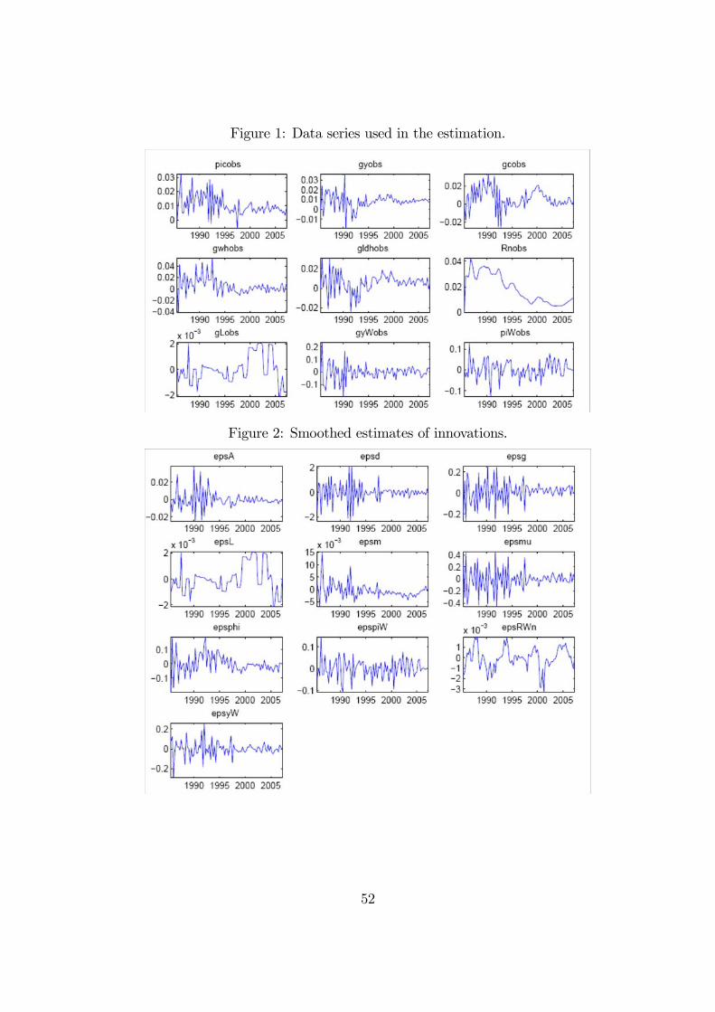
Figure 1: Data series used in the estimation.

Figure 2: Smoothed estimates of innovations.

52

Figure 3: Prior and posterior distributions of the structural parameters.

Figure 4: Prior and posterior distributions of the structural parameters (continued).

53

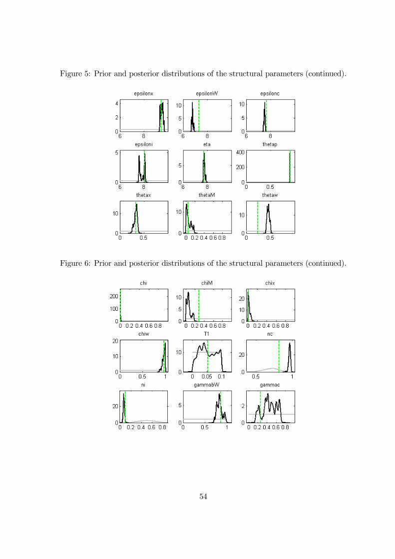
Figure 5: Prior and posterior distributions of the structural parameters (continued).

Figure 6: Prior and posterior distributions of the structural parameters (continued).

54

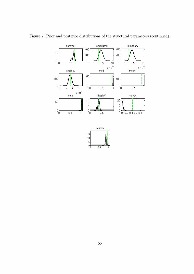
Figure 7: Prior and posterior distributions of the structural parameters (continued).

55

Figure 8: Impulse response function to a transitory general technology shock

Figure 9: Impulse response function to a transitory investment technology shock

56

Figure 10: Impulse response function to a transitory population growth shock

Figure 11: Impulse response function to a transitory labour supply shock

57

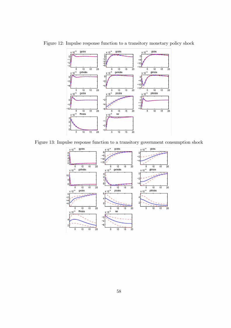
Figure 12: Impulse response function to a transitory monetary policy shock

Figure 13: Impulse response function to a transitory government consumption shock

58

Figure 14: Sources of GDP growth in Spain

-4%

-2%

0%

2%

4%

6%

8%

1986 1988 1990 1992 1994 1996 1998 2000 2002 2004 2006

productivity labourfiscal & monetary policy foreignpreferences GDP

Sources of GDP growth in Spain (in percentage)

Figure 15: Sources of GDP growth in Spain. Labour factor.

-4%

-3%

-2%

-1%

0%

1%

2%

3%

4%

1986 1988 1990 1992 1994 1996 1998 2000 2002 2004 2006

labour supply population labourSources of GDP growth in Spain (in percentage) LABOUR FACTOR

Fuente: INE y Oficina Económica del Presidente

59

Figure 16: Sources of GDP growth in Spain. Technology.

-2%

-1%

0%

1%

2%

3%

1986 1988 1990 1992 1994 1996 1998 2000 2002 2004 2006

investment technology general technology

productivity

Sources of GDP growth in Spain (in percentage) PRODUCTIVITY

Fuente: INE y Oficina Económica del Presidente

Figure 17: Sources of GDP growth in Spain. Foreign factor.

-2%

-1%

0%

1%

2%

1986 1988 1990 1992 1994 1996 1998 2000 2002 2004 2006

world int rate world prices

world demand foreign

Sources of GDP growth in Spain (in percentage) FOREIGN

Fuente: INE y Oficina Económica del Presidente

60

Figure 18: Transitional dynamics after a permanent reduction of 1% in the consumption tax rate.

Figure 19: Transitional dynamics after a permanent reduction in consumption tax rate,

with exogenous monetary policy.

61

Figure 20: Alternative scenario for population growth.

0.0%

0.1%

0.2%

0.3%

0.4%

0.5%

0.6%

1986

1987

1988

1989

1990

1991

1992

1993

1994

1995

1996

1997

1998

1999

2000

2001

2002

2003

2004

2005

2006

2007

population growth (alt esc) population growthsubsamples mean sample mean

Figure 21: Alternative scenario for population growth. Sources of growth.

-4%

-2%

0%

2%

4%

6%

8%

1986 1988 1990 1992 1994 1996 1998 2000 2002 2004 2006

productivity labourfiscal & monetary policy foreignpreferences GDP baselineGDP

Sources of GDP growth in Spain (in percentage)

62