Medchem 528 Biophysical Enzymology and Biopharmaceuticals...

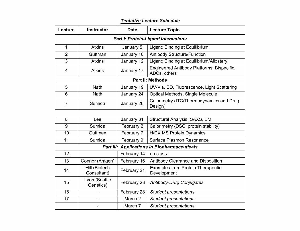
Medchem 528Biophysical Enzymology and Biopharmaceuticals

W, F 3:00 – 4:15 pm

Bill [email protected]

685 0379

Course website:http://courses.washington.edu/medch528

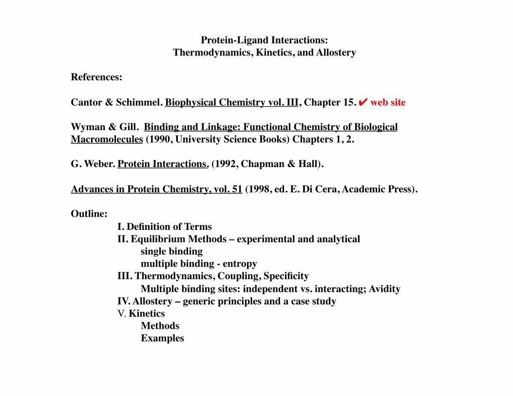
Protein-Ligand Interactions:Thermodynamics, Kinetics, and Allostery

References:

Cantor & Schimmel. Biophysical Chemistry vol. III, Chapter 15. ✔ web site

Wyman & Gill. Binding and Linkage: Functional Chemistry of Biological Macromolecules (1990, University Science Books) Chapters 1, 2.

G. Weber. Protein Interactions. (1992, Chapman & Hall).

Advances in Protein Chemistry, vol. 51 (1998, ed. E. Di Cera, Academic Press).

Outline:I. Definition of TermsII. Equilibrium Methods – experimental and analytical

single bindingmultiple binding - entropy

III. Thermodynamics, Coupling, SpecificityMultiple binding sites: independent vs. interacting; Avidity

IV. Allostery – generic principles and a case studyV. Kinetics

MethodsExamples

I. Ligand Binding: Definition of Terms

The term ‘ligand’ is a problem because of the range of things that must be considered in a unifying theory. ‘Ligands’ include:

electrons

metal ions, other ions

small polar molecules (sugars, nucleotides)

small nonpolar molecules (lipids, steroids)

macromolecules (DNA, proteins, RNA)

‘transition states’

water, a ‘special ligand’

Can there be a general theory for such a broad range of ligands? Something that works for ‘P’ and ‘L’?

I. Definitions (con’t)

units of Ka = liters/mole; units of Kd = moles/liter

for the special case of 1:1 stoichiometry:P + L ⇔ [P • L]

where [L] is free L concentrationFractional occupancy, X is the fraction of total sites occupied by L, and varies with L via a hyperbolic relationship:

and

X varies 0 1 for any stoichiometryvs. ‘number moles L bound/mole protein’ which can be > 1 if multiple binding is present.

Ka =[aAbB][A]a[B]b

aA + bB ⇔ aAbBKd =

1Ka

Kd =[P][L][P • L]

X =[P • L]

[P]+ [P• L]X =

Ka[L]1+ Ka[L]

I. Definitions: thermodynamic terms

For Ka =[aAbB][A]a[B]b

ΔGbind = ΔG°+ -RTlnKa = ΔG°+ RTlnKd

Free energy change for moving reagents from their standard state to the state of comparison; for biochemists, usually pH 7.0, 37 C, but usually ignored.

R = 1.985 calK-1mol-1 = 0.001985 kcalK-1 mol-1

T= temperature in Ke.g. for Kd = 1 micromolar at 37 C, ΔG = (0.001985)(310)ln [1X10-6] = -8.49 kcal/mol.for Kd = 1 nanomolar at 37 C, ΔG = -12.5 kcal/mol. Conversely, 2-fold change in Kd at 37 C is only 0.4 kcal/mol ΔΔG.BIG change in Kd doesn’t require much change in energy.

II. Methods- experimental

The useful parameters that describe the equilibrium are Kd, X, and ΔG.Methods for measuring Kd and X include, but are not limited to:

Partition techniques, in which [L] or [PL] is directly measured (calculate X):

equilibrium dialysis filter binding assays (radiometric) gel filtration

Perturbation Methods, in which a fractional response is measured (Calculate [L]):

absorption, UV-visible spectroscopySurface Plasmon Resonance

fluorescence, CD NMR titration calorimetry

analytical ultracentrifugation

Analytical methods include, but are not limited to, fitting of the data to functions that express X in relation to [L].

hypberbolic plots, Scatchard plots, ‘binding isotherms’, Hill Plots

II. Methods - Analytical Approaches for simple 1:1 binding:Hyperbolic Plot

Scatchard Plots

X

1.0

0

[L]free

0.5

Kd = 1/Ka

X

X =Ka[L]

1+ Ka[L]

X =[P •L]

[P] + [P• L]

X[L]

= Ka − Ka X

X/[L]

X

Slope = 1/-Kd

1.0

these plots tend to distort the data and artificially weight data near the intercepts. Useful qualitatively to seek deviation from linearity, easier than deviation from hyperbola.

II. Methods Analytics “Binding Isotherms”

X

-9 -8 -7 -6 -5 -4 -3

1.0

0

Log Kd

For simple binding, no cooperativity, X = 0.1 to 0.9 spans 1.8 log units.

Preferred method: ΔG is directly proportional to Log [L]. Free energy of the reaction is least ‘sensitive’ to [L] near the Kd. Fractional occupancy is most sensitive in this region,

Log [L]free

Hill PlotsLog [X/(1-X)]

Log [L]free2 0 -2

Log Ka

Log [X/(1-X)] = nLog [L] + Log Ka

Slope = 1 for simple binding where n = 1

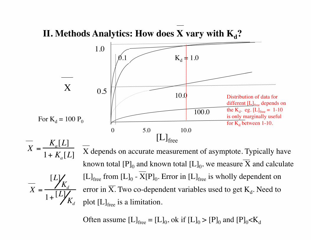
II. Methods Analytics: How does X vary with Kd?

X

[L]free0 5.0 10.0

1.0

0.5

X =Ka[L]

1+ Ka[L]

Kd = 1.00.1

10.0

100.0

X =

[L]Kd

1+ [L]Kd

X depends on accurate measurement of asymptote. Typically have known total [P]0 and known total [L]0, we measure X and calculate [L]free from [L]0 - X[P]0. Error in [L]free is wholly dependent on error in X. Two co-dependent variables used to get Kd. Need to plot [L]free is a limitation.

Often assume [L]free = [L]0, ok if [L]0 > [P]0 and [P]0<Kd

For Kd = 100 P0

Distribution of data for different [L]free depends on the Kd. eg. [L]free = 1-10 is only marginally useful for Kd between 1-10.

II. Analytics and Experimental Design: What determines the experimental range of [L]free or [L]0?

Solubility: Many ligands/proteins are insoluble even in the micromolar range. Limits work at higher concentrations.

Sensitivity: Many techniques are insufficiently sensitive to detect low concentrations. Limits work at low concentrations.

These experimental considerations often oppose each other.

II. Methods Analytics: How does X vary with Kd?Key points:

Experimentally it is critical to use a range of ligand concentrations such that [L]free spans at least two orders of magnitude including data on both sides of Kd, and at least some data need to be at [L]free way above Kd, within ~ 95% of X = 1.0.

Error in X leads to error in both axes of a binding curve – calculation of [L]free from L0 and [PL] is required for the most commonly used analytical expressions but not the most general solution. Error in X can arise if ‘saturation’ is not clearly established – all values on the y-axis are determined by X = 1.0 so if X= 1.0 has error, all y-values have error.

Although [L]free is ‘formally’ required to calculate Kd, at [P0]<< Kd, [L] è [L0]. Total [L] can be a surrogate for decent approximation.

II. Methods:Analytics- Stoichiometric vs. Equilibrium Binding

Consider Kd in terms of what is more easily measurable or known:Kd =

(P0 − [PL])(L0 − [PL])[PL]

0 = [PL]2 − (P0 + L0 + Kd )[PL] + P0L0

( L0P0− X)(1− X) = 0

L0P0

= X

Note symmetrical with respect to L0 and P0, so L and P are ‘interchangeable’

When P0 >> Kd, With algebraic tricks, factoring, substitution, 2 solutions apparent:

That is, the fractional saturation is identical to the molar ratio of L0, P0. The added L binds completely, no [L]free. Plot of X vs. L0 /P0 is linear with slope = 1.

P0, L0 = total protein and total ligand

L0/P0

X

1.0

1.0

P0 = 0.1 Kd

P0 =10Kd

For n = 1, L0/P0 is a max at 1.0. For n > 1, the fraction saturation occurs at L0/P0 = n, the ‘equivalence point’.

Equivalence point yields stoichiometry (n) of binding, but Kd can not be determined directly, because there is no free L. No titration technique can yield both Kd and n from a single experiment. Conditions that yield high precision in Kd have great error in n and vice versa.

Don’t need Lfree, it’s just ‘mathematically’ convenient

II. Methods - analytics for ‘stoichiometric’ binding conditions.

When Kd < P0 the formalism dependent on free [L] breaks down. The full ‘quadratic equation’ resulting from the use of [P]0 - [PL] and [L]0 - [PL] yields the expressions above which when factored yields the new expression for [PL]

Kd =(P0 − [PL])(L0 − [PL])

[PL]

0 = [PL]2 − (P0 + L0 + Kd )[PL] + P0L0

( L0P0− X)(1− X) = 0

L0P0

= X

This ‘general’ equation should be used to calculate Kd if [P]0 > Kd or if there is no way to accurately get [L]free. NOTE: THE QUADRATIC EQUATION Still requires data at low and high [L]0, on both side of the equivalence point.

[P • L] =([P]0 +[L]0 + Kd) − ([P]0 + [L]0 +Kd )

2 − 4[P]0[L]02

II. Methods Analytics: Multiple Binding with Independent Sites: Back to hyperbolic binding: Low [P]Consider a protein with n noninteracting sites, e.g. the IgG or other immunoglobulins. The ‘fractional’ saturation of protein can now be >1. The fractional saturation of protein must be distinguished from fractional saturation of ‘sites.’ More clearly, the number of moles ligand/protein, υ, can be > 1, but the average number of moles ligand/site can still only vary 1 to 0. This has implications for the various analytical solutions, and the information that can be extracted.

fractionalsaturation = υ = n Xii=1

n

∑

υ = nX =nKa[L]1 + Ka[L]

But still a hyperbolic equation! Each of plots above will have the same ’shape’ - can’t detect multiple binding with experiments that measure fractional response. Plots of ‘fractional saturation’ of sites can not yield n directly, n is ‘hidden.’ If you have independent measure of n, can be included to get the real Ka.

Average number of ligands bound/protein

II. Methods Analytics - Multiple noninteracting sites

Lets take a closer look at what contributes to ν

P + L ⇔ PL1

PL1 + L ⇔ PL2

PLn-1 + L ⇔ PLn

K1 =[PL1][P][l]

K2 =[PL2 ][PL1][L]

Kn =[PLn ]

[PLn−1][L]

When n sites/protein, moles L bound/ moles P = ν =

=n i[PLi]i=1∑

[PLi]i= 0

n

∑

=[PL1] + 2[PL2 ] + 3[PL3] + •• •n[PLn ][P] + [PL1] + [Pl2 ] + [PL3] + •••[PLn ]

= nKa[L] 1+Ka[L]

II. Methods- Analytics:Ligand Distribution

When proteins have multiple binding sites, ‘affinity’ or υ are not the only determinants of biological responses to ligands. At subsaturating concentrations of L, their distribution matters. From above we can see that there are multiple ways to distribute, for example, 2 ligands:

Two possibilities that contribute equally to ν

[PL]+[LP] vs. [LPL]

+ +

There are multiple, energetically nondegenerate, ways to distribute a fixed number of ligands. But proteins control this distribution - this is a distinguishing feature of biological systems.

To fully understand ligand distribution we must consider statistical effects, and we must distinguish between macroscopic and microscopic equilibrium constants.

III. Thermodynamics and Statistical Mechanics of Ligand Distribution

Macroscopic vs. Microscopic Equilibrium Constants

How many ways can we arrange ligands among available sites? Consider a protein with 4 identical sites, with 2 ligands to ‘distribute.’:

For n = 4, i = 2, there are 6 species that contribute to [PL2]

From the definition of a binomial distribution in statistics, the number of ways to partition i outcomes with equal probability into n total possible events is:

Ωn,i =n(n −1)(n − 2) ••• (n − i + 1)

i!=

n!(n − i)!i!

III. Thermodynamics of Ligand Binding: Microscopic vs. Macroscopic Binding Equilibria

Consider a diacid, with ionizable groups at either end of an ‘insulating linker’ - so the ends do not ‘sense’ each other:

O-

O

OHOO

O-

OH

O

O

O-O

O-

Ac

OOH

O

OH

Kd1

Kd2

"A"

"AH"

"AH2"

Macroscopic Kd1 = [A]/[AH]

Macroscopic Kd2 = [AH]/[AH2]

Two ways to form AH from A, two ways to lose AH to form AH2

Consider Kd = koff/kon: then

Kd1 = koff/2kon and Kd2 = 2koff/kon

Appears like 4Kd1= Kd2

Statistical effects make Kd1 appear higher affinity even though sites are chemically identical!! Apparent negative cooperativity with respect to proton binding!!

But . . . In an ensemble of proteins with multiple binding sites where we can measure X or ν we can’t see this apparent negative cooperativity. The macroscopic affinity looks uniform, determined by the intrinsic Kd1 = Kd2. Plots are hyperbolic.

X or νAsymptote at 1 or 2

[L]

At low [L] ligands distribute on different P for statistical reasons.

At higher [L], and hence higher X, there is a greater concentration of open sites on P’s already with an L bound. The statistical effect eventually favors binding to the same protein, rather than

different proteins.

III. Thermodynamics, Multiple Binding

III. Thermodynamics - Multiple Binding and entropy as an introduction to the thermodynamics of ligand binding

This statistical effect is an entropic one. The general relationship for n sites is:

Ki =Ω n ,i−1

Ωn ,i

k

S ∝ lnΩ

Here K is the macroscopic dissociation constant for site i, and k is the intrinsic constant. HOMEWORK #1: Calculate the Ki for the 2nd and 3rd ligands binding to a protein with 3 equivalent sites; and for the 2nd, 3rd, and 4th ligands for a protein with 4 equivalent sites. Discuss the result.

Remember that entropy is related to ‘probability.’ Higher entropy of a system at subsaturating ligand is with ligands distributed over many proteins. Entropically unfavorable to ‘park’ many ligands on one protein and none on other proteins.

Entropy works against proteins, by counteracting their ability to control ligand distribution.

S = entropy here (not substrate)

III. Thermodynamics and Ligand Distribution

Consider a ‘ligase’ that joins two substrates, S, into a single larger product. At subsaturating concentrations of S the entropy that favors binding to different proteins results in wasted binding energy. The enzyme population can’t catalyze any reaction if individual enzyme molecules are singly-ligated!

E + S + S [E•S•S] E + S S

But [E•S] + [E•S] can’t do this, only [E • S • S] can. Much of the binding isotherm below saturation would include enzymatically unfunctional complexes. Proteins would be victims of chance (statistics) if they couldn’t control ligand distribution.

The enzyme wants to do this:

Summary of key points so far:•  Parameters needed to describe ligand binding at equilibrium are Kd, X, ΔG.

•  For simple 1:1 binding or for multiple binding at noninteracting sites, Kd should be measured at [P]0<<Kd, using [L]free. Stoichiometry can be measured at [P]0 >> Kd.

•  When [P]0 >> Kd, the Kd must be determined from the ‘quadratic equation’ because there is no [L]free.

•  For multiple noninteracting sites, there is a statistical bias against binding multiple ligands to the same protein molecule, at low [L]. This results from a higher entropic cost.

•  Without a mechanism to control the statistical bias, proteins would be victims of chance at low [L].

III.  Thermodynamics, Coupling Free Energy Consider two distinct ligands L1, L2 with free energy of binding to P, ΔG1 and ΔG2. P can form a ternary complex, and ΔG3 is the free energy of binding L2 to the complex [PL•1] and ΔG4 is the free energy for L1 binding to the complex [PL•2]. We can express this pictorially on a free energy diagram.

P+L1+L2

[P • L1 • L2]

[P•L1]+L2[P•L2]+L1

ΔG1ΔG2

ΔG3ΔG4

ΔG1non+ΔG2non

ΔΔG12

ΔG1+ΔG3 = ΔG2+ΔG4 but no requirement that ΔG1 = ΔG2 or ΔG3 = ΔG4

Required: ΔG4 - ΔG1 = ΔG3 - ΔG2 = ΔΔG12, the coupling free energy

Coupling free energy is the effect that the binding of L1 has on the binding of L2 which must equal the effect that the binding of L2 has on the binding of L1.

P+L1+L2

[P • L1 • L2]

ΔG

III. Thermodynamics, coupling free energy

ΔΔG12

If ΔΔG12 = 0, ligands have no effect on each other, no cooperativity

If ΔΔG12 < 0 , then ΔG of binding two ligands simultaneously is more negative, more favorable, than individual ligands, positive cooperativity.

If ΔΔG12 > 0, then ΔG of binding individual ligands is more positive, less favorable, than binding two ligands simultaneously, negative cooperativity.

P+L1+L2

[P • L1 • L2]

[P•L1]+L2[P•L2]+L1

ΔG1ΔG2

ΔG3ΔG4

ΔG1+ΔG2

P+L1+L2

[P • L1 • L2]

III. Thermodynamics, CouplingThe coupling free energy is critically important in biology - it determines ligand distribution and biological response. It can be considered in another thermodynamic context. The ΔΔG12 is equal to the ΔG for the disproportionation reaction:

[P • L1] + [P • L2] P + [L1 • P • L2] where Keq =[P • L1 •L2][P][L1 •P][P • L2 ]

Consider the case when [L1] and [L2] are adjusted to X1 = X2 = 1/2

If X 1 =

[P• L1] +[P • L1 •L2]P0

X 2 =[P• L2] + [L1 •P • L2]

P0 X 1,2 =

[P • L1 • L2]P0

Then at X 1 = X 2 = 1/2 Keq =[X 1,2 ]2

(1/ 2 − [X 1, 2]) 2

and X 1,2 =

1/ 2 Keq

(1+ Keq )

Knowing that ΔΔG12 = -RTlnKeq we can solve for ΔΔG12 in terms of X12

€

ΔΔG12 = −RT ln2X 1,2

[1− 2X 1,2]

III. Thermodynamics, coupling

for [P • L1] + [P • L2] P + [L1 • P • L2]

A few special features: when ΔΔG12 = 0, no coupling, half the ligands L1 are in [L1P] or [L1PL2] and half the L2 ligands are in [PL2] or [L1PL2], so X1,2 = 0.25 at zero coupling. Note, as coupling is favorable (more negative ΔΔG12) there is an increase in X1,2, the fraction of protein with two ligands bound, and vice versa. Also, using known values of RT, ~90% of P is P or [L1PL2] at -2.75 kcal/mol and 90% is [L1P + PL2] for ΔΔG12 +2.75 kcal/mol.

X1,20 0.5

ΔΔG12

(kcal/mol)

-2.75

0

+2.75

This plot tells us that very good coupling (90% toward one side) can be obtained for small ΔΔG12, on the order of 3 kcal/mol or - 3 kcal/mol. For the price of a hydrogen bond proteins can get very good control of ligand distribution. On the other hand, due to the asymptotic nature of the plot, with respect to ΔΔG12 = 0 and ΔΔG1,2 = 0.5, it is very expensive to get perfect control.

€

ΔΔG12 = −RT ln2X 1,2

[1− 2X 1,2]

0.05 0.45

III. Thermodynamics, coupling

Of course there can be homotropic cooperativity as well, directly analogous to the heterotropic case above.

P+L1+L1

[P • L1 • L1]

[P•L1]+L1ΔG1

ΔG2

ΔG1+ΔG2

P+L1+L1

[P • L1 • L1][P • L1 • L1]ΔG2

Positive cooperativity: ΔG1+ΔG2< 2ΔG1

Negative cooperativity:

ΔG1 +ΔG2 > 2ΔG1

No cooperativity:

ΔG1+ΔG2 = 2ΔG1

III. Thermodynamics, cooperativity and linkageThe previous free energy diagrams emphasize the path-independent nature of the state function ΔG, and hence of binding affinity. They can be recast in the framework of a thermodynamic box.

Because of the path independence, and in relation to the coupling free energy, it is obvious that any effect that L2 has on the binding of L1 must be equal to the effect that L1 has on the binding of L2. This reciprocity was first discussed in the context of hemoglobin, O2, and CO by Hendersen, and Wyman elaborated a theory of thermodynamic ‘linkage’ based on chemical potential (rather than ΔG).

δ(lnX2)/ δX1 = δ(lnX1)/ δX2

L1+P+L2 [L1•P]

[P • L2] [L1 • P • L2]

Kd1

Kd2

Kd3 Kd4

Kd1Kd4 = Kd2Kd3

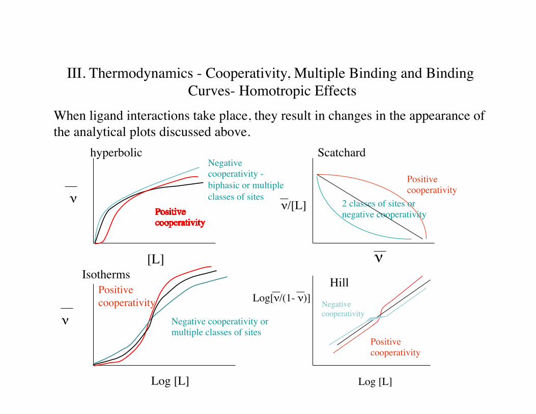
III. Thermodynamics - Cooperativity, Multiple Binding and Binding Curves- Homotropic Effects

When ligand interactions take place, they result in changes in the appearance of the analytical plots discussed above.

ν

[L]

hyperbolicNegative cooperativity -biphasic or multiple classes of sites

ν/[L]

ν

Scatchard

2 classes of sites or negative cooperativity

Positive cooperativity

ν

Log [L]


Negative cooperativity or multiple classes of sites

Isotherms

Log[ν/(1- ν)]

Log [L]


HillNegative cooperativity

III. Thermodynamics and intra-ligand cooperativity: the basis for specificity.

Consider two parts of a single ligand, rather than two separate ligands. Binding of each part is ‘coupled’ to the other parts, and hence binding of the parts is cooperative.

ligand

enzymeΔG1

ΔG2

ΔG3

ΔG4

ΔG2’ ΔG1’

ΔG1+ΔG3 = ΔG2+ΔG4 < ΔG2’ + ΔG1’ due to lower entropy cost, once part of a molecule is bound.

Unfavorable entropy of binding already paid when the first part binds.

III. Thermodynamics, coupling: An example of a therapeutic protein

Enbrel marketed first by Immunex (Seattle) in 1998 is an example of the use of coupling free energy, via bivalency. TNF mediates rheumatoid arthritis. A strategy to reduce systemic TNF was to ‘sponge’ it up with a soluble TNF receptor construct. TNF is a trimer of identical subunits and the TNF receptor (TNFR) was known to bind at a subunit-subunit interface of the trimer. Immunex fused a soluble fragment of TNFR to the Fc region of an IgG, thus resulting in a ‘bivalent’ TNFR. A blockbuster drug!

sTNFR

Fc TNF

Kd = 5 nM

Kd = 45 nM

TNF and Enbrel, structures

enbrel

sTNFR

Fc

Trimeric TNF

sTNFR

Mukai et al, Science Signaling vol 3, 143, 2010

III. Thermodynamics, coupling: Enbrel as an example of bivalency.

ΔG1Kd = 45 nM

Kd =

5 nM

ΔG2

45nM

ΔG2Kd = 45 nM

ΔG1

ΔΔG12

TNF + sTNFR TNF + Enbrel

ΔG3

ΔG1+ΔG2 > ΔG1+ΔG3, positive cooperativity between 2 sTNFR Kd = 45 nM: ΔG = -10.4 kcal/mol

Kd = 5 nM;

ΔG = -11.7 kcal/mol and ΔΔG = - 1.3 kcal/mol

III. Thermodynamics, coupling - bivalent inhibitorsWhile the concept of ‘multivalency’ has been appreciated in drug design circles for a long time, recent advances in high throughput NMR and computational methods have brought into focus as ‘fragment-based drug discovery.’

FBDD uses NMR/computation to screen libraries of ‘small fragments’ that bind simultaneously to a target. Lead Fragments with the best ‘ligand efficiency’ are linked together to create a ‘multivalent’ lead compound. This is exploitation of coupling free energy.

Bcl-xl

III. Thermodynamics, bivalent inhibitors, linker considerations

The ‘entropic advantage’ of multivalency is only realized if the linker is entropically neutral. Both the binding elements (fragments) and linker forfeit conformational, rotational, translational, vibrational degrees of freedom when they bind. If the linker is long and flexible, the entropic cost of binding the linker offsets any advantage from the multivalency. Best linkers are short. For long flexible linkers, their conformational distribution becomes an important design element, and they also contribute directly to enthalpic interactions with the protein.

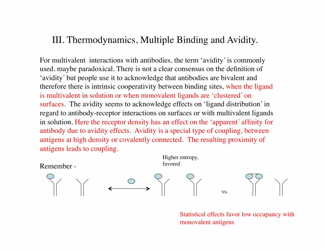
III. Thermodynamics, Multiple Binding and Avidity.

For multivalent interactions with antibodies, the term ‘avidity’ is commonly used, maybe paradoxical. There is not a clear consensus on the definition of ‘avidity’ but people use it to acknowledge that antibodies are bivalent and therefore there is intrinsic cooperativity between binding sites, when the ligand is multivalent in solution or when monovalent ligands are ‘clustered’ on surfaces. The avidity seems to acknowledge effects on ‘ligand distribution’ in regard to antibody-receptor interactions on surfaces or with multivalent ligands in solution. Here the receptor density has an effect on the ‘apparent’ affinity for antibody due to avidity effects. Avidity is a special type of coupling, between antigens at high density or covalently connected. The resulting proximity of antigens leads to coupling.

Remember -

vs.

Higher entropy, favored

Statistical effects favor low occupancy with monovalent antigens

III. Thermodynamics of ‘Avidity’On Surfaces

KdApp = Kd' X Kd"

Kd' = s'k Kd" = s"k

surface bound antigens

if antigen density is appropriate KdApp < Kd' or Kd"

In Solution

KdApp = Kd' X Kd"

n-2n-2

n-2

if antigen antigen density is appropriate KdApp < Kd' or Kd"

With antigens immobilized on surfaces, such as on cells (receptors) or on SPR chips, the antigens now ‘appear’ multivalent. In effect the cell surface or the SPR chip surface is the ‘linker.’ The properties of the surface and the density of antigens can result in apparent increases in affinity (avidity). Thus the measurement of antibody affinity on cells and in SPR experiments can be tricky.

Each part of the step-wise binding process has statistical effects (‘s’ terms) that vary with antigen density. Unlike statistical effects in multivalent proteins with monovalent ligands, the statistical effects can now cause ‘apparent positive cooperativity’ which is conceptually analogous to the multivalent examples above (FBDD).

Similar considerations in solution if antigen is multivalent, as with Enbrel above.

Read: Mack et al. (2012) Thermodynamic Analysis to Assist in the Design of Recombinant Antibodies.Crit Rev Immun 32: 503-527.

IV. Allostery - ‘other site’ Allostery is the useful exploitation of control of ligand distribution for some biological advantage. Although we are now comfortable with the concept of allostery, it was controversial when first proposed in the early 1960’s. A ‘traditional’ analytical approach is the application of the Hill plot, as described above. Whereas we already considered the ‘’stepwise’ nature of multiple ligand binding, Hill considered multiple ligand binding as a two state process, in distinct contrast to all the examples above which explicitly recognize intermediate states of ligation.

P + nL↔ P •nL Ka =[P •nL][P][L]n

X =[P •nL][P]total

=[L]n

[L]n + Kd

log X (1− X )"

# $ %

& ' = logKd + n log[L]

Hill considered the slope, n, as the cooperativity index - a perfectly cooperative system with stoichiometry n would yield a line of slope n. As a result, n, has often mistakenly been used as a measure of stoichiometry. The Hill model is physically unreasonable and no ‘physical’ meaning can be applied to the Hill coefficient. It is however a useful comparator of the degree of cooperativity for a system with known or fixed ‘n’.

Log[X/(1-X)]

Log [L]

Slope n

IV. AllosteryTwo observations initiated the development of allosteric models: 1) for some systems non-hyperbolic binding curves were observed; 2) Some pairs of ligands of Aspartate transcarbamoylase (ATC) acted ‘noncompetitively’ as inhibitors or as activators of one another.

The two most thoroughly studied allosteric systems are Hemoglobin and ATC, which fostered the ‘textbook’ models. These models remain extremely useful although we now know they are imperfect.

Because these models exemplify possible mechanisms by which proteins control ligand distribution and the resulting biological utility, it is useful to briefly review them.

In particular, these models emphasize that ligand binding is coupled to conformational change in the same way multiple ligand binding is coupled. Conformational change provides the coupling free energy that ligands exhibit.

IV. Allostery - Hemoglobin and the Monod-Wyman-Changeux Model

Assumptions of the MWC model:

•  Binding sites are distributed symmetrically, they have equivalent positions within the protein structure.

•  each subunit has separate binding sites for different ligands.

• Protein has two conformational ‘states’ in equilibrium, and ligands have a greater affinity for one state.

•  macroscopic affinity of ligands is a function of the conformational equilibrium.

L L = [T0]

[R0]

Apologize - here L is an equilibrium constant, X is a ligand - the formalism in textbooks is often this way.

R0 T0

L L = [T0]

[R0]

kr =

kr1 = kr2= kr3 = kr4

kt =

kt1 = kt2= kt3 = kt4

R0+X RX1

RX1+X RX2

RX2+X RX3

RX3+X RX4

T0+X TX1

TX1+X TX2

TX2+X TX3

TX3+X TX4

IV. Allostery, hemoglobin and the MWC model, for n = 4

kr ≠ kt, but define ‘c’, ckt = kr, so when c< 1, X binds R0 more tightly than T0

The degree of cooperativity is determined by c, L, n

Intrinsic dissociation constants

High affinity Low affinity

R1 T1

R2 T2

etc

Don’t need to explicitly consider these equilibria, they are defined by c, L in a ‘thermodynamic box sense.’

X =i(Ri ) + i(Ti )

i =1

n

∑i =1

n

∑

n i(Ri) + i(Ti)i =1

n

∑i =1

n

∑"

# $ %

& '

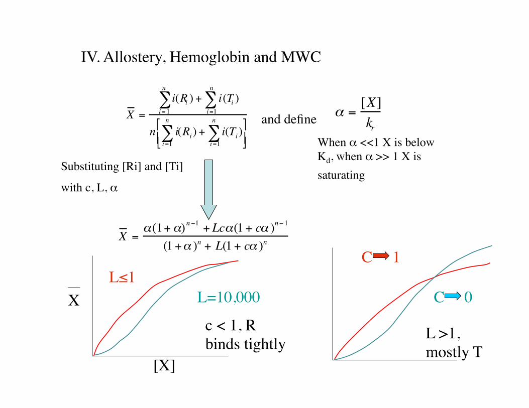
α =[X]kr

X =α(1+α)n−1 + Lcα(1+ cα )n−1

(1+α )n + L(1+ cα )n

and define

When α <<1 X is below Kd, when α >> 1 X is saturating Substituting [Ri] and [Ti]

with c, L, α

X

[X]

c < 1, R binds tightly

L≤1L=10,000

L >1, mostly T

C 1

C 0

IV. Allostery, Hemoglobin and MWC

IV. Allostery- effects of L and c on response

X =α(1+α)n−1 + Lcα(1+ cα )n−1

(1+α )n + L(1+ cα )n α =

[X]kr

ckt = kr ; L = [T0]/[R0]

X

[X]X =

α (1+α)3

(1+α )4 + L

Note: when L = 0, X = α(1 +α)

A hyperbola, when only 1 conformation!

Consider, n = 4, c = 0, L>>1, nearly all T state, which doesn’t bind X:

Case 1: For this case, when α<<1, X approaches α/L, a line of slope 1/L.

Case 2: For the case α ≈ 1<<L,

X =α + 3α 2 + 3α 3 + α4

L

Case 3: For the case α = L>>1

X = (L4)/(L+L4) 1

1.0

Greatest sigmoidicity when L>>1, c<<1, low X and mid X depend on L

α(1+α)3

IV. Allostery, the MWC model

Note that cooperativity is observed even though no ligand affects the affinity (Kd) of any subsequent ligands. kr and kt are constant!

Where is the coupling free energy?

The cooperativity arises because addition of ligand, ‘pulls’ the

R ⇔ T equilibrium towards R, the high affinity state - this increases the concentration of high affinity sites, it doesn’t change their affinity. The coupling energy comes from the linkage between ligand binding and the conformational equilibrium defined by L. For any concentration ratio [T]/[R] along the way the distribution of ligands among the R population and separately among the T population is determined by statistical effects.

IV. Allostery, Limitation of the MWC model

A major shortcoming of the MWC model is its thermodynamic incompatibility with negative homotropic cooperativity.

Any binding of a ligand must result in a greater population of the high affinity form, at the expense of the low affinity form. How could this lead to negative cooperativity?

If kr < kt, Lx must be < L because Lkr = ktLx

Negative cooperativity not possible!

L L = [T0]

[R0]

kr ktIf c = .1, ligand 10 times more likely to bind R. In order to maintain L, more R must be generated - more high affinity sites available.Lx

R0 T0

IV. Allostery, an alternative model: Adair, Koshland, Nemethy, Filmer or the ‘Koshland Model’A less restrictive model is the ‘Koshland’ model or the ‘sequential’ model of allostery, which allows for sequential conformational changes in individual subunits rather than concerted conformational change. No assumptions regarding symmetry are included - negative homotropic cooperativity is allowed.

K1 K2 K3 K4

K1<K2<K3<K4, pure positive homotropic cooperativity

K1>K2>K3>K4, pure negative homotropic cooperativity

Other combinations, mixed cooperativity

All allowed because each state is different from those states on either side.

Note however, that each subunit only exists in two states (pure induced fit).

IV. Allostery, A completely general model: Nested allosteryA more general model allows for multiple subunit conformations in each ligand state. This is particularly relevant for large multisubunit complexes with multiple types of subunits. Ligand binding is coupled to conformational change - this is the entire basis of cooperativity and allostery.

MWC

Koshland

IV. Allostery: Hemoglobin (Hb) as an example of optimized control of ligand distribution.

X

pO2

Tetramer with DPG

dimer

Hb exists as an α2β2 tetramer, of αβ dimers

Dimers have reduced cooperativity, but bind O2 more tightly than tetramers

O2 induced dissociation of Tetramers into αβ dimers in vitro

X-ray structures of oxy vs deoxy Hb reveal 2 quaternary states, R and T with major differences at the α1β1/α2β2 interface

Despite lots of structural info about Hb allostery, the energetics remained uncertain through 1970’s – 80’s.

stripped tetramer

IV. Allostery, Hb as an example: The Symmetry Rule for HbThrough heroic efforts by Ackers et al. and Edelstein et al. combined with x-ray structures the intermediate states of ligation of Hb have been characterized structurally and energetically (thermodynamically). Much of this analysis has exploited the fact that αβ dimers of Hb can be isolated and studied, and exploiting the fact that tetramer dissociation into dimers is coupled to oxygen (ligand) binding.Strategy of calculating ligand binding coupling energy from subunit association data:Take a step back, and consider ligand binding to a homodimer of monomers M: cooperativity of ligand binding to the dimer (ΔG21 - ΔG22) can be obtained from the difference in subunit affinities in the absence and presence of ligand X (ΔG2-ΔG1)

2M + 2X

M2 + 2X

MX + M + X

MX + XM

Liga

nd b

indi

ng to

mon

omer

s

Ligand binding to dimers

M2X + X

M2X2

ΔG11

ΔG11

ΔG0

ΔG1

ΔG2

ΔG0 = energy for monomer association in the absence of X; ΔG21-ΔG11 = energy for monomer association with one X bound; ΔG22-ΔG11 = energy for monomer association with two X bound. ΔG2 - ΔG0 = ΔG21 – ΔG22 – coupling free energy

of ligand binding is equal to coupling free energy of monomer association in the absence vs presence of ligand.

Remember, experimentally difficult to isolate M2X and add X, therefore difficult to measure coupling free energy between ligand binding with ligand titrations. But may be experimentally easy to measure ΔG0 and ΔG2.

ΔG21

ΔG22

This strategy was used by Ackers et al for the heterodimers in tetrameric hemoglobin. Obviously this is even more complicated with heterodimers. They could isolate αβ dimers with either α or β subunits substituted with metalloporphyrins that don’t bind ligand, and they use CN- ion as a tight binding surrogate for oxygen that didn’t rearrange or redistribute. Together this allowed them to know which subunit in the dimer or tetramer was binding ligand (-CN) and to assume that the ligand didn’t ‘hop’ around (no ligand redistribution).

IV. Allostery, Hb as an example: The Symmetry Rule for Hb

heme

α Subunit

β subunit

ligand

ΔGα

ΔGβ

0ΔGa

2ΔGa

ΔGα + ΔGβ + ΔΔG12

Similarly for other arrangements of ligands and: ΔG for dimerization of doubly ligated states differed with distribution of ligands

IV. Allostery, Hb as an example: The Symmetry Rule for HbCollectively the data suggested a model of nested allostery where individual monomers can undergo tertiary rearrangement without global quaternary switching. Global T R switching occurs only after 1 subunit in each αβ dimer binds oxygen. Therefore, Hb does not strictly satisfy the MWC model. In the mid 1990’s, Ackers proposed this symmetry rule. Think about the implications of the nested vs MWC model.

α1 β2

β1 α2T, low affinity

R, high affinity

The cooperativity is not ‘symmetrical. Cooperativity is greater between 2nd and 3rd and 3rd and 4th binding events, than between 1st and 2nd. The first and second binding events are subject to ‘statistical’ effects, whereas the protein controls later stages of binding via cooperativity.

1st binding event does not change dimer interface and hence does not change quaternary structure.

2nd binding event changes quaternary structure if and only if it includes occupancy by at least 1 subunit in each dimer. Statistics control that, including chance of binding to other tetramers.

IV. Allostery, Hb and asymmetric cooperativity: the latest model

Through additional efforts in 2003-2005 Ackers et al revised the symmetry rule. In fact there is positive intradimer cooperativity - the tetramer does not rely on statistical effects other than in the very first binding step.

Cooperativity is symmetric with respect to ligation state- not the caseAsymmetric cooperativity

Homework. Read and summarize (2 pages) the experimental strategy and important results in: Ackers et al. SCIENCE 255: 54-63 (1992)Ackers and Holt, JBC 281: 11441-11443 (2006)

IV. Allostery, Hb cooperativity is asymmetricThe physiologic implications of this remain unclear, other than minor tweeking.

1. The significance of the overall cooperativity is obvious - more efficient unloading of O2 at the O2 concentrations in tissue, after loading in the lungs. Hb has evolved to optimize loading of O2 at its ambient pressure in the lungs and unload it at only a modestly lower (2.5-fold) pO2 in tissue. Compare to a hyperbolic binding curve, wherein a 6-8-fold decrease in [L] to achieve a 2.5-fold decrease in X. ALSO, The asymmetry may promote interactions with other effectors??

2. Indeed as a result of the asymmetric cooperativity, binding curves for Hb are asymmetric. The asymmetry further enhances ability of Hb to ‘unload’ O2 from its saturated state even with only a small drop in ‘ligand concentration’ (pO2). The binding curve is slightly steeper on the high saturation side than on the low saturation side. Hb control of the sequence of events is more subtle, clever, than the symmetry rule implies.

http://www.youtube.com/watch?v=2L1UJgYH6bU

‘A molecular dance in the blood, observed’

Medchem 528 Biophysical Enzymology and Biopharmaceuticals...

Documents

Transcript of Medchem 528 Biophysical Enzymology and Biopharmaceuticals...