Mechanics of viscous wedges: Modeling by analytical and ...

Mechanics of viscous wedges: Modeling by analytical and

numerical approaches

Sergei MedvedevDepartment of Oceanography, Dalhousie University, Halifax, Nova Scotia, Canada

Received 10 January 2001; revised 25 November 2001; accepted 30 November 2001; published 26 June 2002.

[1] Although complex rheological models have been used to study the evolution oforogenic wedges, many features of simple models remain to be fully explained. Here,we analyze the plane strain evolution of model orogenic wedges under simpleboundary and rheological conditions. The uniform linear viscosity wedge is driven bymotion of a basal boundary at a constant velocity. Three main analysis techniques areused: analytical (algebraic analysis of scales involved), semianalytical (thin sheetapproximation), and a complete numerical approach. Application of this variety ofapproaches provides a better understanding of the underlying physics and outlines theadvantages and disadvantages of the different techniques. The evolution of wedges canbe divided into three phases. Initially, wedge growth is mainly vertical andsymmetrical and depends little on the viscosity. The second phase exhibits almost self-similar growth with the appearance of surface extension, within an otherwisecompressional system, and development of asymmetry. The last phase involveswidening of wedge and further development of asymmetry and surface extension, theaverage slope of wedge decreases during this phase. The Ramberg number, the ratio ofcharacteristic gravitational to shear stress, defines the duration of each phase. Severalparameters introduced here (mean surface slope, asymmetry of the wedge, surfaceextension, and near-surface strain history) allow observations from natural wedges tobe linked to the bulk viscosity of the model wedges. Analysis shows that the thinsheet approximation does not correctly describe the initial stages of wedgeevolution. INDEX TERMS: 8020 Structural Geology: Mechanics; 8102 Tectonophysics: Continental

contractional orogenic belts; 8122 Tectonophysics: Dynamics, gravity and tectonics; 8164 Tectonophysics:

Stresses—crust and lithosphere; KEYWORDS: orogenic wedge, thin-sheet approximation, numerical

modelling, scaling analysis, extension, contraction

1. Introduction

[2] The behavior of viscous models of the lithosphere inthe context of plate tectonic convergence provides someinsights into the dynamics of the growth of orogenicwedges. In previous work, viscous material has been usedin analogue models [Buck and Sokoutis, 1994] and variousnumerical [Ellis et al., 1995; Royden, 1996; Willett, 1999;Shen et al., 2001] and analytical [Emerman and Turcotte,1983; Platt, 1986, 1993, 2000; Buck and Sokoutis, 1994;Ellis, 1996] investigations. Several interpretations based onfield studies of accretionary prisms emphasize the relevanceof the viscous model for the internal deformation of wedges[Ring and Brandon, 1999; Feehan and Brandon, 1999].Buck and Sokoutis [1994], Royden [1996], and Willett[1999] demonstrated that a uniform linear-viscous orogenicwedge can exhibit surface extension as the result of theconvergent basal boundary motion, which may explain

normal sense shear features of several orogenic zones (seeexamples from Willett [1999]).[3] Even though many studies have modeled the evolu-

tion of orogenic wedges using more complex rheologies[e.g., Beaumont et al., 1994, 1996, 2000; Ellis et al., 1998],some features of the underlying simple models remainunclear. The purpose of present work is to improve ourunderstanding of the behavior of uniform linear viscouswedges by identifying analytically the key parameterscontrolling their growth.[4] The boundary and initial conditions for the formation

of an asymmetric doubly-vergent wedge (Figure 1a) werechosen for analysis owing to their simplicity and becausethey are the same as those used by Buck and Sokoutis[1994] and Willett [1999]. By choosing uniform linearviscosity and time-invariant boundary conditions we limitthe problem to only a few free parameters listed in the firstpart of Table 1.[5] In simplifying the model some processes that accom-

pany orogenesis, such as isostasy and erosion, have beenneglected. The time range at which the approach can beused is also limited. The boundary conditions chosen also

JOURNAL OF GEOPHYSICAL RESEARCH, VOL. 107, NO. B6, 10.1029/2001JB000145, 2002

Copyright 2002 by the American Geophysical Union.0148-0227/02/2001JB000145$09.00

ETG 9 - 1

preclude direct application of this model to accretionarywedges, where a basal decollement and/or rear backstopsignificantly influence the evolution [e.g., Platt, 1993].Although the complexities of natural systems restrict directquantitative comparison with the model results, qualitativesimilarities exist [e.g., Royden, 1996; Willett, 1999].[6] We investigate the evolution of several wedge proper-

ties that can be compared directly to geological observationsand data, such as shape of the wedge (rate of growth,average slopes, and asymmetry), and the instantaneousand finite surface strains (Figure 1b and Table 1). Severalapproaches are used for analysis and modeling:1. Scaling analysis roughly estimates forces acting in the

system and the mass balance. Two analytical models arepresented in this work: AM1 (section 2.1) and AM2/AM2h(section 3.4).2. Details of the evolution cannot be obtained analyti-

cally; therefore numerical models are needed. The simplestpossible numerical model is based on the thin sheetapproximation, the SS approach (‘‘simple shear,’’ followingclassification presented by Medvedev and Podladchikov[1999a]). Although this approach has been used before todescribe orogenesis [Emerman and Turcotte, 1983; Lob-kovsky and Kerchman, 1991; Buck and Sokoutis, 1994],some new insights into this approach are discussed here(section 2.2).3. The results and conclusions based on the approximate

techniques listed above are tested by reference to a morecomplete numerical model based on the finite elementapproach containing the complete balance of forces, the PSapproach (‘‘plane strain’’ [Fullsack, 1995], section 2.3).

[7] Application of these different approaches not onlyprovides a better understanding the physical processescontrolling the evolution of wedges but also allows insightinto the limitations of different approaches. The mainemphasis here is on the SS approach, which is widely usedin geodynamics. However, the major simplificationsimplicit in this method require a more systematic inves-tigation of the consequent limitations and applicability thanhas been done to date [Royden, 1996; Medvedev andPodladchikov, 1999a, 1999b].[8] The first part of the paper presents approaches used to

investigate the model. The second part concerns the evolu-tion of wedge shape and classification of the differentphases of evolution. The third part presents the evolutionof surface strains and strain rates.

2. Methods

2.1. Analytical Model (AM1): Scaling Analysis

[9] The model described here is based on rough estima-tions of forces and mass balance. The horizontal forcebalance in the wedge for the case of a horizontal base andstress-free upper surface is

�F1 þ F2 � Ft ¼ 0; ð1Þ

where the forces are shown on Figure 2. The forces inequation (1) can be estimated from the bulk stresses in thewedge:

F1 ¼Z h0

0

sxxjx¼1dz � 1

2rgh20;

F2 ¼Z h0þ�h

0

sxxjx¼0dz � 1

2rg h0 þ�hð Þ2 þ 2m

V

leh; ð2Þ

Ft ¼Z x1

0

sxzjz¼0dx � 1

2mVeh l;

where indexed s denotes the components of the stresstensor and eh = h0 + 0.5�h is the average thickness of thewedge assuming a triangular geometry. The averagedhorizontal strain rate can be estimated as V/l, which isthen used to estimate the viscous part of F2.[10] An estimation of basal shear stress used in the

expression for Ft is made as follows. First, the averagedvertical variation of horizontal velocity was estimated as adifference between basal velocity, V, and the averagevelocity at the top surface of the prowedge (V/2). Thisvariation divided by averaged thickness of wedge, eh, andmultiplied by viscosity results in averaged shear stress in theprowedge. As shear stress is zero at the top surface, theshear stress along the base can be estimated as twice theaverage.[11] Substitution of equation (2) into equation (1) gives

rg�hehþ 2mV

ehl� 1

2mV leh ¼ 0;

or ð3ÞFg þ Fn � Ft ¼ 0;

Figure 1. (a) Basic wedge model. Initial and boundaryconditions include stress-free upper surface and basalvelocity, V(x), which is constant (V+ or V�) and hassingularity at x = 0. The base is horizontal and fixed. Lateralboundaries extend beyond the deformation. Initial layerthickness is h0, and layer material has constant vis-cosity, m,and density, r (Table 1). (b) Deformed wedge. Length scaleof deformation, l, is divided to l+ and l� representingscales for two sides of the wedge; wedge shape is measuredby thickness, h(x, t), and maximum uplift,�h = max (h� h0)located at xmax. See Table 1 for other parameters.

ETG 9 - 2 MEDVEDEV: MECHANICS OF VISCOUS WEDGES

where Fg approximates the gravity forces acting in thewedge (this term relates to the gradient of potentialenergy [Jones et al., 1996]); Fn estimates the influence ofhorizontal compressional viscous stresses in the systemdue to advection of mass into the wedge; and Ftrepresents shear stresses acting along the base of thewedge. The dimensionless ratio, the Ramberg number[after Ramberg, 1981; Weijemars and Schmeling, 1986],

Rm ¼ rgh20=mV ð4Þ

is used to relate gravitational stresses acting in the modelto the basal shear stress (see Table 1). Elsewhere, thisratio was termed the Argand number in other basallydriven wedge problems [Buck and Sokoutis, 1994; Willett,1999]. However, the Argand number was introduced byEngland and McKenzie [1982] as ratio of gravitational(buoyancy) to horizontal compressional stresses, not shearstresses. Rm is used here to distinguish the difference inthe physics behind these numbers. To illustrate thisdifference, we also construct the Argand number (Table 1)according to the England and McKenzie [1982] defini-tion, but it is related to a horizontal length scale l, whichcannot be readily estimated from the initial and/orboundary conditions and in further developments we donot refer to values of Ar.

[12] The range of values of Rm used in the furtheranalyses is illustrated in Table 2. Values of Rm higherthan 20 result in very wide wedges, while geologicalsituations with Rm lower than 1 are unlikely. We nowscale all parameters to be dimensionless using the scales

Table 1. Parameters of the Viscous Wedge Problem

Parameter Definition, CommentsSI Units

[Dimensional Scale]Variations Analyzed[Range of Results]

Setup ParametersH* length scale, H* = h0 m 5–40 kmg acceleration due to gravity m/s2 10 m/s2

V* velocity, V* = abs(V+ � V�) m/s 0.1–4 cm/yrm* viscosity Pa s 1020–1023Pa sr* density kg/m3 (2�3.3) 103 kg/m3

Characteristic Valuess*g gravitational stress Pa r*gH*s*t shear stress Pa m*V*/H*s*n normal stress Pa m*V*/lt* convergence time, time needed to converge the system by

horizontal distance of one characteristic length scale (H*)s H*/V*

t*e evolution time (equation (12)) sffiffiffiffiffiffiffiffiffiffiffiffiffiffiffiffiffiffiffiffim*=r*gV*

pDimensionless Complexes

Rm = s*g/s*t Ramberg number, ratio of gravity to shear stresses (equation (4), Table 2) – 1–20Ar = s*g/s*n Argand number, ratio of gravity to normal stresses – –

Variablesa

h(x, t) actual thickness of the layer (Figure 1b) [H*] [1–3]L(t) width of zone of finite extension along the top surface (Figure 11b) [H*] [0–5]t dimensional time [t*], [te*]

t0 = t/t* dimensionless time corresponding to the total convergence in units ofthe initial thickness h0

– 0–30

t0e = t/t*e dimensionless time corresponding to stages of evolution (equation (12),Figure 14)

– 0–30

V(x) basal velocity: V = 0 for x < 0 and V = �V* for x > 0 (Figure 1a) [V*] 0–V*xmax(t) horizontal position of maximum uplift of wedge (Figure 7b) [H*] [0–1]ea(t) tangent of mean slope of wedge (equation (11), Figure 5) – [0–0.3]�h(t) maximum uplift in the system, max(h � h0) (Figure 3b and 3d) [H*] [0–2]e(x, t) surface strain, positive e indicates finite extension – [up to 100%]e(i, t) strain evolution of certain, ith, Lagrangian element (Figure 12) – [up to 100%]l width of wedge, horizontal length scale of deformation (equation (6)) [H*] [2–80]

l+(t), l�(t) widths of prowedge and retrowedge, l+ + l� = l (Figure 7a) [H*]aDimensionless variables are marked by primes. They can be rescaled to dimensional equivalents by multiplying by the dimensional scales from this table.

Figure 2. Horizontal forces acting on the prowedge.Wedge is assumed to be geometrically symmetric (l+ �l� � l/2). Region x � x1 is undeformed; therefore noviscous stresses contribute to force F1. Average thickness ofthe wedge is eh � h0 + �h/2, and mean slope is ~a = �h/l+.

MEDVEDEV: MECHANICS OF VISCOUS WEDGES ETG 9 - 3

presented in the Table 1. For example, the averaged thick-ness of the wedge becomes eh0 = 1 + �0

h/2. Equation (3) thenbecomes

Rm�0

h

l0 þ 2

l0ð Þ2� 1

2 eh0� �2 ¼ 0; ð5Þ

demonstrating the control of the force balance by Rm.[13] Assuming that the wedge has a triangular shape, the

total mass balance can be expressed in dimensional and[dimensionless] forms:

�hl=2 � tVh0; �0hl

0=2 � t0� �

ð6Þ

where dimensionless time t0 characterizes the amount ofadvected material (see Table 1). The system of equations(5) and (6) for the first analytical model, AM1, has twounknowns, l(t) and �h(t) that can be calculated analyti-cally and used to predict the evolution of the most generalproperties such as height and width of the wedge, andaveraged forces acting in the wedge (see section 3.3 andsection 4.2). The main limitation of AM1 is that thegeometry and boundary conditions are symmetric aboutx = 0.

2.2. Thin Sheet Approximation (Model SS):Semianalytical Approach

[14] Semianalytical methods used to investigate the evo-lution of a wedge include so-called thin sheet approxima-tions. These models attempt to calculate analytically thevertical distributions of stresses based on the geometricassumption that the ratio of the vertical to horizontal lengthscales in the model is small.[15] The SS (‘‘simple shear’’) approach is based on the

lubrication approximation to the Stokes equations. Appliedto the problem of this work, Stokes equations of motion indimensionless form give

Rm@P 0

@x 0� @2v 0x

@ z 0ð Þ2� @2v 0x

@ x 0ð Þ2

" #¼ 0

Rm@p0

@z0þ 1

� �� @2v 0z

@ x 0ð Þ2þ @2v 0z

@ z 0ð Þ2

" #¼ 0;

ð7Þ

where primes indicate dimensionless values (Table 1), P isthe pressure, and vx(x, z) and vz(x, z) are horizontal andvertical velocities. Scaling the mass forces (rg) in the secondequation results in the ‘‘1.’’ The SS approach assumes thatvariations in the horizontal direction are much smaller thanin the vertical direction and that the vertical velocity issmaller than horizontal velocity. This results in neglecting

the terms in brackets, which means neglecting the normalviscous stresses in the horizontal balance of forces andassuming pressure to be lithostatic (see complete asymptoticanalysis by Zanemonetz et al. [1976]; Lobkovsky andKerchman [1991]; Medvedev [1993]; and Medvedev andPodladchikov [1999b]). After omitting terms in brackets,equations (7) represent the lubrication approximation[Schlichting, 1979; Emerman and Turcotte, 1983]. Integra-tion of the simplified equations (7) gives a parabolicvariation of horizontal velocity with depth:

v0x x0; z0ð Þ ¼ V 0 � Rmz0 2h0 � z0ð Þ

2

@h0

@x0; ð8Þ

see Table 1 for definition of terms. Combining the integratedvelocity profile with mass conservation results in a simpledescription of wedge evolution by a single equation [e.g.,Buck and Sokoutis, 1994]:

@h0

@t0þ @

@x0V 0h0ð Þ � Rm

@

@x0h0ð Þ3

3

@h0

@x0

!¼ 0: ð9Þ

Note that the form of the SS approach presented byequations (8) and (9) assumes a fixed, flat base (z = 0).The essence of the physics behind this approach is that thegravitational spreading of the wedge is balanced by the shearstress in the layer.[16] Our analytical model AM1 (section 2.1, equation

(5)) includes three types of forces in the balance; gravita-tional, normal viscous, and shear viscous. The SS approachneglects normal viscous stresses. Thus AM1 can be recog-nized as more complete qualitatively but cannot handle anydetailed analysis. Numerical treatment based on the SSapproach can give detailed results, but the implications ofthe assumptions behind this approach should be tested. TheSS approximation is believed to be acceptable if thehorizontal length scale of the problem is much greater thanthe vertical scale [Zanemonetz et al., 1976; Medvedev,1993]. In the next sections we will investigate the accuracyof this assumption.

2.3. Numerical Approach: Plane Strain Finite ElementMethod (PS)

[17] This method is based on the finite element discreti-zation of the complete balance of forces, its formulationdoes not imply any simplifying assumptions. Therefore thismethod is used as a reference, and all our conclusions havebeen tested against this approach.[18] The numerical code involves an arbitrary Lagran-

gian-Eulerian formulation. The finite element calculation ofvelocities is performed on an Eulerian grid that undergoeslittle distortion as the wedge grows. The Lagrangian grid isused to track deformations and to advect material properties[Fullsack, 1995]. This code [Fullsack, 1995] has been testedand used extensively [e.g., Beaumont et al., 1994, 1996,2000; Willett, 1999]. Several types of finite element inter-polations (e.g., bilinear 4 nodes, quadratic 9 nodes, Crou-zeix-Raviart 7 nodes and Pian-Sumihara 4 nodes [Cuvelieret al., 1986; Zienkiewicz and Taylor, 1989]) have beenimplemented and tested against analytical solutions, andresults for different elements were compared to ensure

Table 2. Limiting Parameter Values Used to Calculate Range of

Rm

Rmr,

kg/m3h0,km

V,cm/yr

m,Pa s

Strong crust 1 3100 35 1 1023

Sediments 20 2800 5 1 1020


correctness (P. Fullsack, personal communications, 1999–2000).

3. Results

[19] Results presented here are the solutions for theproblem described by Figure 1 for the asymmetricdoubly-vergent wedge. The ideas and solutions of ana-lytical (AM1 and AM2) and semianalytical (SS)approaches are tested by comparison with numericalresults of the full finite element approach (PS). Figurespresent results obtained by the PS approach unlessotherwise specified.

3.1. Evolution of Wedge Shape: Dependence on Rm

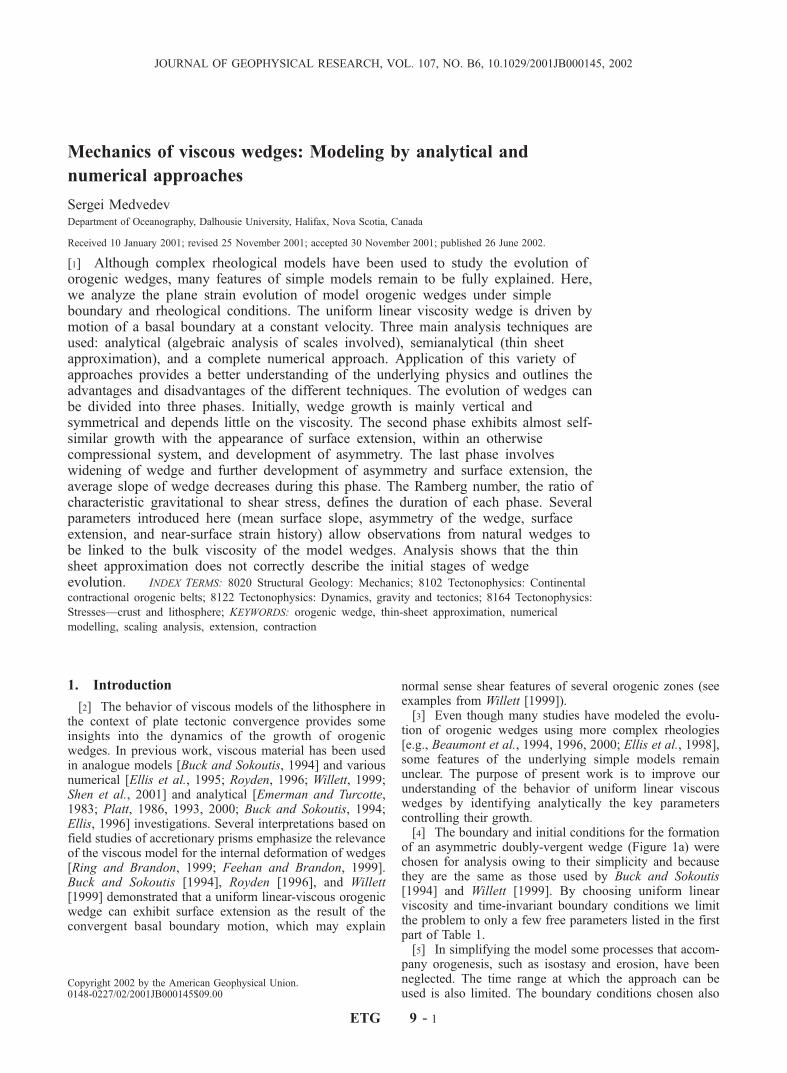
[20] Initially, for small uplift (�h � h0), equation (5)concludes that l is nether much smaller nor much greaterthan h0 and that the first term of equation (5) is muchsmaller than the other two. Thus the solution is onlyweakly dependent on Rm. This conclusion is supportedby the PS numerical results (Figures 3a and 3b). Thisinitial stage is shorter the larger the Rm (equation (5)), andit can be seen (Figures 3b and 3d) that the results aredistinct for the range of Rm used here when t0 � 0.4,where t0 (Table 1) is the dimensionless time. More evolvedmodels (Figures 3c and 3d) exhibit large differences instyles depending on Rm.[21] The width of deformation can be estimated by l0(t)

2t0/�0h (equation (6)) using Figures 3b and 3d. This gives

l � 5h0 for the initial stage (t0 = 0.1 to 0.3) independent of

Rm and with a very low dependence on time (Figure 3a).During the later stages the width, l, varies with time and

Rm. For example, the width ranges from 8h0 to 25h0 at t0 = 4

depending on Rm (Figure 3c).

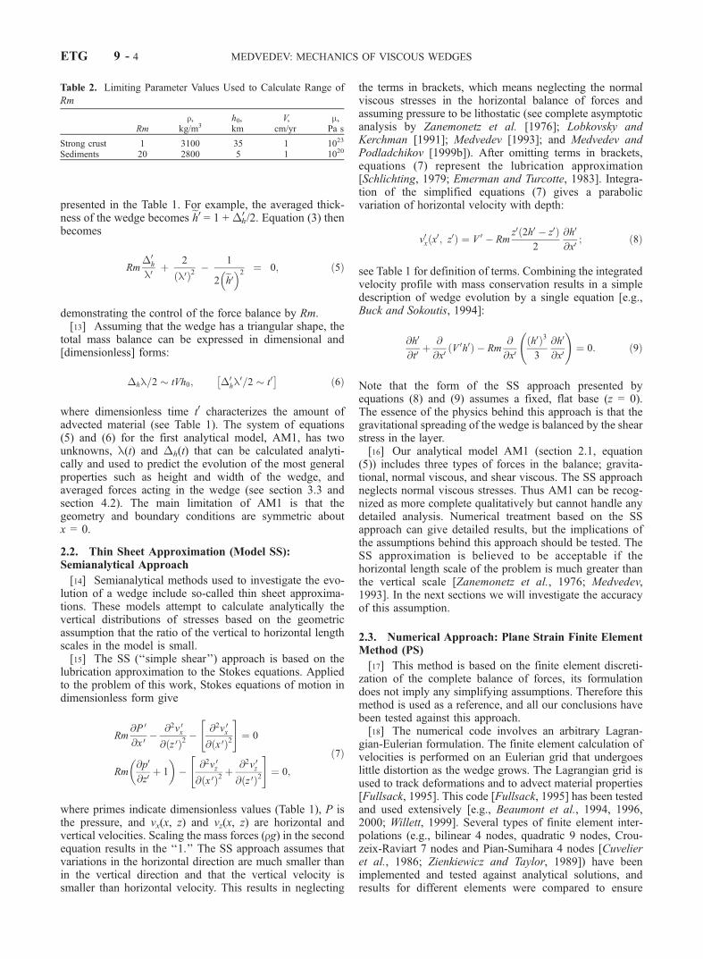
3.2. Comparison With Thin Sheet Approximations

[22] In this section we compare results of the complete PSmodeling approach with results obtained by the SS thinsheet approximation and analyze this comparison usingother approaches. The accuracy of thin sheet approxima-tions is directly related to the smallness of the vertical tohorizontal length-scale ratio [Zanemonetz et al., 1976;Medvedev, 1993], which is usually defined by the initialand/or boundary conditions of a problem. However, theproblem considered here does not have predefined horizon-tal length scale (Figure 1a). To estimate the accuracy, wecompare the AM1 and SS approaches. The term neglectedby the SS approach in the horizontal balance of forces(equations (7)) corresponds to the term Fn from the inte-grated balance included in the AM1 approach (equation(5)). Dividing equation (5) by Fn and using the dimension-less form of equation (6) gives the following form of thehorizontal force balance:

1

2Rm t0 þ 1� l0=2eh0� �2

¼ 0 ð10Þ

Here the term neglected by the SS approach appears as ‘‘1,’’and therefore the SS approximation can be valid only if boththe first and the third terms in equation (10) are muchgreater than 1. The latter condition corresponds to thetraditional criteria for thin sheet approximations that thewidth of deformation is much larger than the height.However, this condition applies to the results of finite

Figure 3. Topography and thickness of wedges with different Rm. In the initial phase (Figures 3a and3b) the dependence on Rm is low, which contrasts with the later phases (Figures 3c and 3d). (a and c)Nondimensional topography versus position at nondimensional time shown by dashed line (Figures 3band 3d). (b and d) Normalized maximum elevation versus time. Note vertical exaggeration (Figures 3aand 3c).


deformation and these length scales are not predefined. Theratio l0/eh0 does, however, grow with time and the accuracyof thin sheet approximation therefore increases (seecomparison for Rm = 1 on Figure 4d).[23] The condition Rm t0 � 1 also results in accuracy

increasing with time but requires special considerationduring the initial phase. When t0 � 0, the SS approxima-tion is inaccurate because the first term of equation (10) isalso �0. This phase is, however, short for high Rm. Hencethe accuracy is poor for low Rm (Rm = 1, Figures 4a, 4b,and 4d) but is good for large Rm (Rm =10, Figures 4c and4d; see also comparison of the SS approach with ananalogue experiment of Buck and Sokoutis [1994] whereRm = 10).

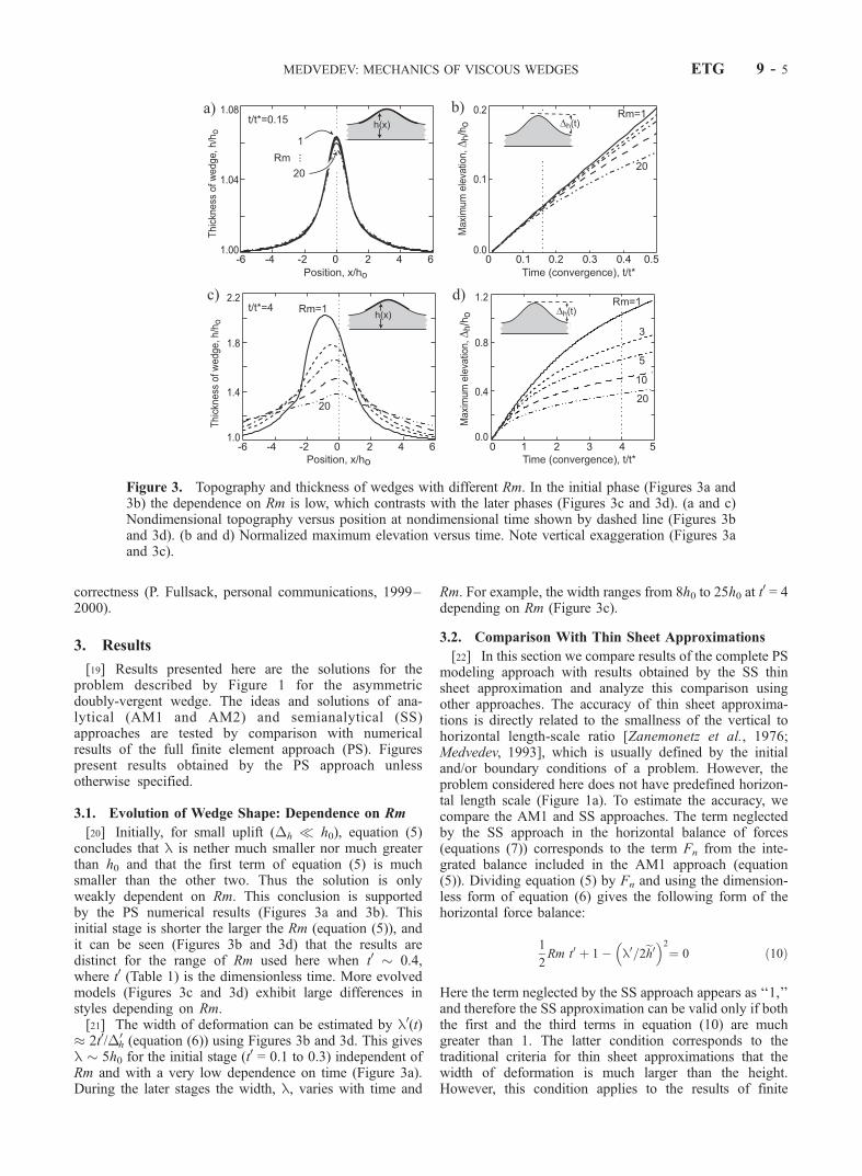
3.3. Evolution of Mean Slope

[24] How slopes of the wedge evolve with convergence isa characteristic property of the wedge. Investigations in thissection are based on the ‘‘mean slope,’’ ea, of the wedge;defined as the ratio of the characteristic uplift of the system,�h, to half of the characteristic width, l/2 (Figures 2 and5a). Using equation (6), ea can be estimated for a symmetricwedge by

ea ¼ �h

l=2¼

�0h

� �2t0

¼ �2h

th0V: ð11Þ

Applying this equation to asymmetric wedges results resultsin ea as an average value of the two slopes in the wedge.

[25] For AM1, equations (5) and (6) can be used toestimate time dependence of the mean slope analytically.The result for Rm = 1 (Figure 5a) shows three phases: I,initially the wedge growth is mostly vertical, therebyincreasing ea; II, wedge growth is almost self-similar withnear constant ea; III, finally, the wedge spreads horizontallyand ea decreases.[26] AM1 results predict that as Rm is increased, the

maximum ea is reached earlier (the same behavior is alsoshown by PS results, Figure 5b). The time when the slope isa maximum, tmax, can be estimated with good accuracyfrom the empirical condition tmax

ffiffiffiffiffiffiffiRm

p const. This allows

us to introduce the characteristic evolution time for thewedge, t*e, as

t*e ¼ t*. ffiffiffiffiffiffiffi

Rmp

¼

ffiffiffiffiffiffiffiffiffiffiffiffiffim*

r*gV*

sð12Þ

and the new dimensionless evolution time, te = t0ffiffiffiffiffiffiffiRm

p.

The robustness of the evolution time is illustrated by thefact that the scaled times of maximum slope (indicated byarrow heads on Figure 5c) for different Rm occur in theinterval te 4.3–5.3. Using the scaling parameters pre-sented in Table 2, the corresponding dimensional time tmax

varies from �1 Myr for ‘‘sediments’’ to �10 Myr for‘‘strong crust’’ models.[27] The SS approach results in monotonically decreasing

mean slope (Figure 5a, the initial part, for t0 < 2, of thiscurve is out of scale of the graph). This slope can, however,

Figure 4. Comparison of wedge results obtained by the PS (solid line) and SS (dashed line) approachesfor different phases of convergence: (a and b) initial and (c and d) developed shown as in Figure 3. ForRm = 1 the SS approach at the initial stages (Figures 4a and 4b) is inaccurate, while it improves for largert0 = t/t* (Figures 4c and 4d). Accuracy of SS also depends on Rm: higher values give better agreementwith accurate PS solutions (Figures 4c and 4d). Note also that in the SS solution the point of maximumuplift is always at x = 0, while the PS solution demonstrates retroward shift.


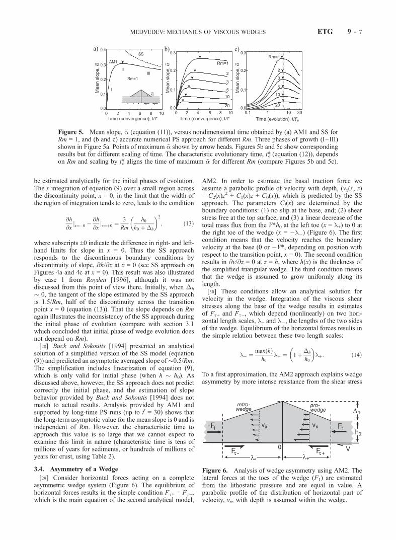
be estimated analytically for the initial phases of evolution.The x integration of equation (9) over a small region acrossthe discontinuity point, x = 0, in the limit that the width ofthe region of integration tends to zero, leads to the condition

@h

@xjx¼�0 �

@h

@xjx¼þ0 ¼

3

Rm

h0

h0 þ�h

� �2

; ð13Þ

where subscripts ±0 indicate the difference in right- and left-hand limits for slope in x = 0. Thus the SS approachresponds to the discontinuous boundary conditions bydiscontinuity of slope, @h/@x at x = 0 (see SS approach onFigures 4a and 4c at x = 0). This result was also illustratedby case 1 from Royden [1996], although it was notdiscussed from this point of view there. Initially, when �h

� 0, the tangent of the slope estimated by the SS approachis 1.5/Rm, half of the discontinuity across the transitionpoint x = 0 (equation (13)). That the slope depends on Rmagain illustrates the inconsistency of the SS approach duringthe initial phase of evolution (compare with section 3.1which concluded that initial phase of wedge evolution doesnot depend on Rm).[28] Buck and Sokoutis [1994] presented an analytical

solution of a simplified version of the SS model (equation(9)) and predicted an asymptotic averaged slope of�0.5/Rm.The simplification includes linearization of equation (9),which is only valid for initial phase (when h � h0). Asdiscussed above, however, the SS approach does not predictcorrectly the initial phase, and the estimation of slopebehavior provided by Buck and Sokoutis [1994] does notmatch to actual results. Analysis provided by AM1 andsupported by long-time PS runs (up to t0 = 30) shows thatthe long-term asymptotic value for the mean slope is 0 and isindependent of Rm. However, the characteristic time toapproach this value is so large that we cannot expect toexamine this limit in nature (characteristic time is tens ofmillions of years for sediments, or hundreds of millions ofyears for crust, using Table 2).

3.4. Asymmetry of a Wedge

[29] Consider horizontal forces acting on a completeasymmetric wedge system (Figure 6). The equilibrium ofhorizontal forces results in the simple condition Ft+ = Ft�,which is the main equation of the second analytical model,

AM2. In order to estimate the basal traction force weassume a parabolic profile of velocity with depth, (vx(x, z)= C2(x)z

2 + C1(x)z + C0(x)), which is predicted by the SSapproach. The parameters Ci(x) are determined by theboundary conditions: (1) no slip at the base, and; (2) shearstress free at the top surface, and (3) a linear decrease of thetotal mass flux from the V*h0 at the left toe (x = l+) to 0 atthe right toe of the wedge (x = �l�) (Figure 6). The firstcondition means that the velocity reaches the boundaryvelocity at the base (0 or �V*, depending on position withrespect to the transition point, x = 0). The second conditionresults in @v/@z = 0 at z = h, where h(x) is the thickness ofthe simplified triangular wedge. The third condition meansthat the wedge is assumed to grow uniformly along itslength.[30] These conditions allow an analytical solution for

velocity in the wedge. Integration of the viscous shearstresses along the base of the wedge results in estimatesof Ft+ and Ft�, which depend (nonlinearly) on two hori-zontal length scales, l+ and l�, the lengths of the two sidesof the wedge. Equilibrium of the horizontal forces results inthe simple relation between these two length scales:

l� ¼ max hð Þh0

lþ ¼ 1þ�h

h0

� �lþ: ð14Þ

To a first approximation, the AM2 approach explains wedgeasymmetry by more intense resistance from the shear stress

Figure 6. Analysis of wedge asymmetry using AM2. Thelateral forces at the toes of the wedge (F1) are estimatedfrom the lithostatic pressure and are equal in value. Aparabolic profile of the distribution of horizontal part ofvelocity, vx, with depth is assumed within the wedge.

Figure 5. Mean slope, ~a (equation (11)), versus nondimensional time obtained by (a) AM1 and SS forRm = 1, and (b and c) accurate numerical PS approach for different Rm. Three phases of growth (I–III)shown in Figure 5a. Points of maximum ~a shown by arrow heads. Figures 5b and 5c show correspondingresults but for different scaling of time. The characteristic evolutionary time, t*e (equation (12)), dependson Rm and scaling by t*e aligns the time of maximum ~� for different Rm (compare Figures 5b and 5c).


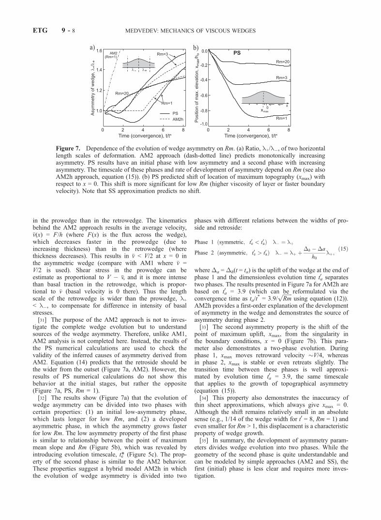
in the prowedge than in the retrowedge. The kinematicsbehind the AM2 approach results in the average velocity,�v(x) = F/h (where F(x) is the flux across the wedge),which decreases faster in the prowedge (due toincreasing thickness) than in the retrowedge (wherethickness decreases). This results in �v < V/2 at x = 0 inthe asymmetric wedge (compare with AM1 where �v =V/2 is used). Shear stress in the prowedge can beestimate as proportional to V � �v, and it is more intensethan basal traction in the retrowedge, which is propor-tional to �v (basal velocity is 0 there). Thus the lengthscale of the retrowedge is wider than the prowedge, l+< l�, to compensate for difference in intensity of basalstresses.[31] The purpose of the AM2 approach is not to inves-

tigate the complete wedge evolution but to understandsources of the wedge asymmetry. Therefore, unlike AM1,AM2 analysis is not completed here. Instead, the results ofthe PS numerical calculations are used to check thevalidity of the inferred causes of asymmetry derived fromAM2. Equation (14) predicts that the retroside should bethe wider from the outset (Figure 7a, AM2). However, theresults of PS numerical calculations do not show thisbehavior at the initial stages, but rather the opposite(Figure 7a, PS, Rm = 1).[32] The results show (Figure 7a) that the evolution of

wedge asymmetry can be divided into two phases withcertain properties: (1) an initial low-asymmetry phase,which lasts longer for low Rm, and (2) a developedasymmetric phase, in which the asymmetry grows fasterfor low Rm. The low asymmetry property of the first phaseis similar to relationship between the point of maximummean slope and Rm (Figure 5b), which was revealed byintroducing evolution timescale, te* (Figure 5c). The prop-erty of the second phase is similar to the AM2 behavior.These properties suggest a hybrid model AM2h in whichthe evolution of wedge asymmetry is divided into two

phases with different relations between the widths of pro-side and retroside:

Phase 1 symmetric; t0e < t0að Þ l� ¼ lþ

Phase 2 asymmetric; t0e > t0að Þ l� ¼ lþ þ�h ��a

h0lþ;

ð15Þ

where�a =�h(t = ta) is the uplift of the wedge at the end ofphase 1 and the dimensionless evolution time t0a separatestwo phases. The results presented in Figure 7a for AM2h arebased on t0a = 3.9 (which can be reformulated via theconvergence time as ta/t

* = 3.9/ffiffiffiffiffiffiffiRm

pusing equation (12)).

AM2h provides a first-order explanation of the developmentof asymmetry in the wedge and demonstrates the source ofasymmetry during phase 2.[33] The second asymmetry property is the shift of the

point of maximum uplift, xmax, from the singularity inthe boundary conditions, x = 0 (Figure 7b). This para-meter also demonstrates a two-phase evolution. Duringphase 1, xmax moves retroward velocity �V/4, whereasin phase 2, xmax is stable or even retreats slightly. Thetransition time between these phases is well approxi-mated by evolution time t0a = 3.9, the same timescalethat applies to the growth of topographical asymmetry(equation (15)).[34] This property also demonstrates the inaccuracy of

thin sheet approximations, which always give xmax = 0.Although the shift remains relatively small in an absolutesense (e.g., 1/14 of the wedge width for t0 = 8, Rm = 1) andeven smaller for Rm > 1, this displacement is a characteristicproperty of wedge growth.[35] In summary, the development of asymmetry param-

eters divides wedge evolution into two phases. While thegeometry of the second phase is quite understandable andcan be modeled by simple approaches (AM2 and SS), thefirst (initial) phase is less clear and requires more inves-tigation.

Figure 7. Dependence of the evolution of wedge asymmetry on Rm. (a) Ratio, l+/l�, of two horizontallength scales of deformation. AM2 approach (dash-dotted line) predicts monotonically increasingasymmetry. PS results have an initial phase with low asymmetry and a second phase with increasingasymmetry. The timescale of these phases and rate of development of asymmetry depend on Rm (see alsoAM2h approach, equation (15)). (b) PS predicted shift of location of maximum topography (xmax) withrespect to x = 0. This shift is more significant for low Rm (higher viscosity of layer or faster boundaryvelocity). Note that SS approximation predicts no shift.


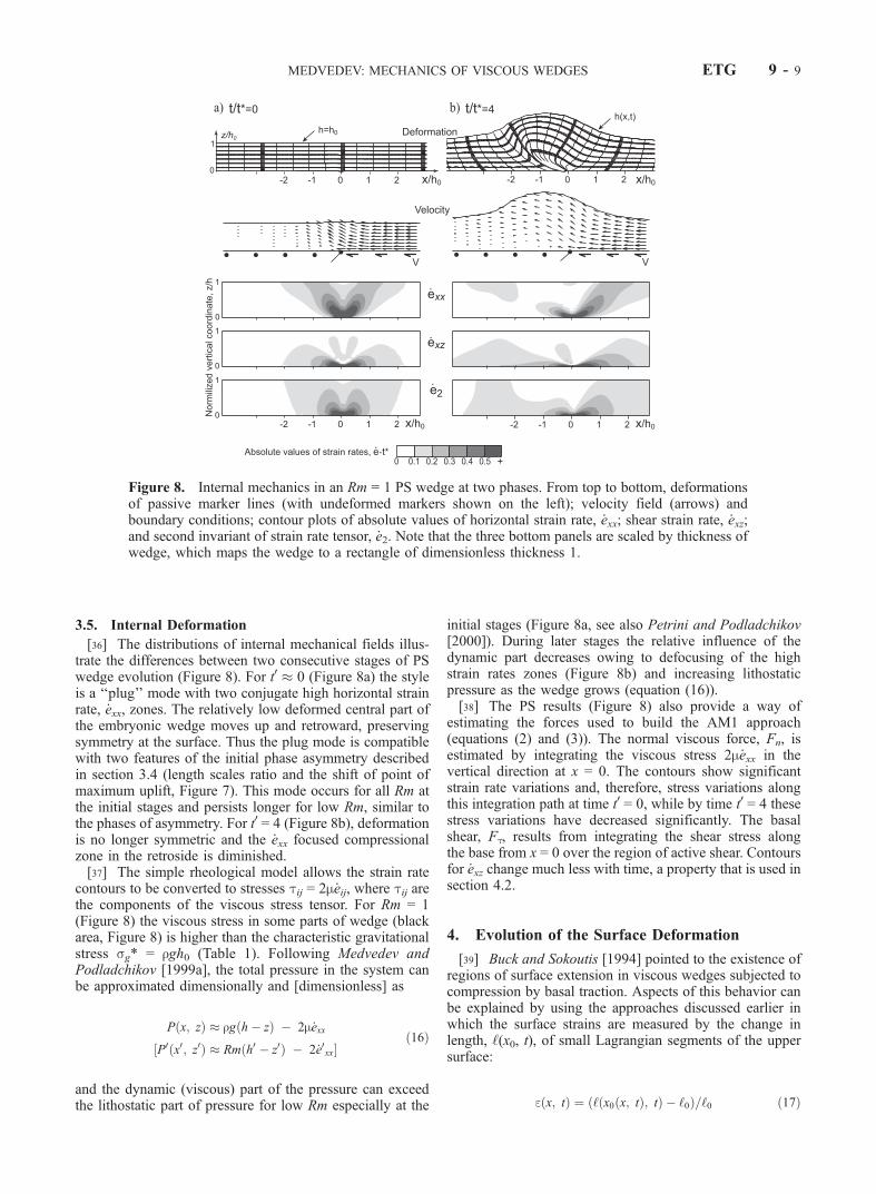
3.5. Internal Deformation

[36] The distributions of internal mechanical fields illus-trate the differences between two consecutive stages of PSwedge evolution (Figure 8). For t0 0 (Figure 8a) the styleis a ‘‘plug’’ mode with two conjugate high horizontal strainrate, _exx, zones. The relatively low deformed central part ofthe embryonic wedge moves up and retroward, preservingsymmetry at the surface. Thus the plug mode is compatiblewith two features of the initial phase asymmetry describedin section 3.4 (length scales ratio and the shift of point ofmaximum uplift, Figure 7). This mode occurs for all Rm atthe initial stages and persists longer for low Rm, similar tothe phases of asymmetry. For t0 = 4 (Figure 8b), deformationis no longer symmetric and the _exx focused compressionalzone in the retroside is diminished.[37] The simple rheological model allows the strain rate

contours to be converted to stresses tij = 2m _eij, where tij arethe components of the viscous stress tensor. For Rm = 1(Figure 8) the viscous stress in some parts of wedge (blackarea, Figure 8) is higher than the characteristic gravitationalstress sg* = rgh0 (Table 1). Following Medvedev andPodladchikov [1999a], the total pressure in the system canbe approximated dimensionally and [dimensionless] as

P x; zð Þ rg h� zð Þ � 2m _exx

P0 x0; z0ð Þ Rm h0 � z0ð Þ � 2 _e0xx½ �ð16Þ

and the dynamic (viscous) part of the pressure can exceedthe lithostatic part of pressure for low Rm especially at the

initial stages (Figure 8a, see also Petrini and Podladchikov[2000]). During later stages the relative influence of thedynamic part decreases owing to defocusing of the highstrain rates zones (Figure 8b) and increasing lithostaticpressure as the wedge grows (equation (16)).[38] The PS results (Figure 8) also provide a way of

estimating the forces used to build the AM1 approach(equations (2) and (3)). The normal viscous force, Fn, isestimated by integrating the viscous stress 2m _exx in thevertical direction at x = 0. The contours show significantstrain rate variations and, therefore, stress variations alongthis integration path at time t0 = 0, while by time t0 = 4 thesestress variations have decreased significantly. The basalshear, Ft, results from integrating the shear stress alongthe base from x = 0 over the region of active shear. Contoursfor _exz change much less with time, a property that is used insection 4.2.

4. Evolution of the Surface Deformation

[39] Buck and Sokoutis [1994] pointed to the existence ofregions of surface extension in viscous wedges subjected tocompression by basal traction. Aspects of this behavior canbe explained by using the approaches discussed earlier inwhich the surface strains are measured by the change inlength, ‘(x0, t), of small Lagrangian segments of the uppersurface:

e x; tð Þ ¼ ‘ x0 x; tð Þ; tð Þ � ‘0ð Þ=‘0 ð17Þ

Figure 8. Internal mechanics in an Rm = 1 PS wedge at two phases. From top to bottom, deformationsof passive marker lines (with undeformed markers shown on the left); velocity field (arrows) andboundary conditions; contour plots of absolute values of horizontal strain rate, _exx; shear strain rate, _exz;and second invariant of strain rate tensor, _e2. Note that the three bottom panels are scaled by thickness ofwedge, which maps the wedge to a rectangle of dimensionless thickness 1.


where ‘0 is the initial length of the small segment. Thisapproach differs from that used by Willett [1999], who onlytake horizontal changes into account. The main difference isseen in the extension for low Rm, which can be negligiblewhen only the horizontal component is used.

4.1. Surface Strain Rates

[40] A necessary condition for finite surface extension isan extensional strain rate along the surface. Variations ofsurface strain rates for conditions similar to those presentedhere and for different rheologies and boundary conditionsare given by Royden [1996] and Willett [1999]. Here weemphasize only one property of the surface (z = h) strainrates derived from the SS approach (equation (8)):

_exxjz¼h ¼ @v0 x; hð Þ@x

: ¼ �Rmh0ð Þ2

2

@2h0

@ x0ð Þ2� Rm h0

@h0

@x0

� �2

;

ð18Þ

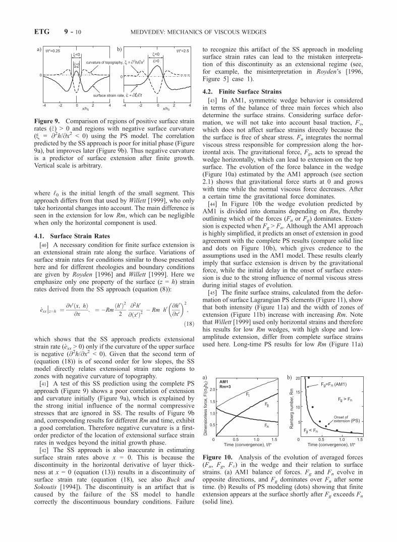
which shows that the SS approach predicts extensionalstrain rate ( _exx > 0) only if the curvature of the upper surfaceis negative (@2h/@x2 < 0). Given that the second term of(equation (18)) is of second order for low slopes, the SSmodel directly relates extensional strain rate regions tozones with negative curvature of topography.[41] A test of this SS prediction using the complete PS

approach (Figure 9) shows a poor correlation of extensionand curvature initially (Figure 9a), which is explained bythe strong initial influence of the normal compressivestresses that are ignored in SS. The results of Figure 9band, corresponding results for different Rm and time, exhibita good correlation. Therefore negative curvature is a first-order predictor of the location of extensional surface strainrates in wedges beyond the initial growth phase.[42] The SS approach is also inaccurate in estimating

surface strain rates above x = 0. This is because thediscontinuity in the horizontal derivative of layer thick-ness at x = 0 (equation (13)) results in a discontinuity ofsurface strain rate (equation (18), see also Buck andSokoutis [1994]). The discontinuity is an artifact that iscaused by the failure of the SS model to handlecorrectly the discontinuous boundary conditions. Failure

to recognize this artifact of the SS approach in modelingsurface strain rates can lead to the mistaken interpreta-tion of this discontinuity as an extensional regime (see,for example, the misinterpretation in Royden’s [1996,Figure 5] case 1).

4.2. Finite Surface Strains

[43] In AM1, symmetric wedge behavior is consideredin terms of the balance of three main forces which alsodetermine the surface strains. Considering surface defor-mation, we will not take into account basal traction, Ft,which does not affect surface strains directly because thethe surface is free of shear stress. Fn integrates the normalviscous stress responsible for compression along the hor-izontal axis. The gravitational force, Fg, acts to spread thewedge horizontally, which can lead to extension on the topsurface. The evolution of the force balance in the wedge(Figure 10a) estimated by the AM1 approach (see section2.1) shows that gravitational force starts at 0 and growswith time while the normal viscous force decreases. Aftera certain time the gravitational force dominates.[44] In Figure 10b the wedge evolution predicted by

AM1 is divided into domains depending on Rm, therebyoutlining which of the forces (Fn or Fg) dominates. Exten-sion is expected when Fg > Fn. Although the AM1 approachis highly simplified, it predicts an onset of extension in goodagreement with the complete PS results (compare solid lineand dots on Figure 10b), which gives credence to theassumptions used in the AM1 model. These results clearlyimply that surface extension is driven by the gravitationalforce, while the initial delay in the onset of surface exten-sion is due to the strong influence of normal viscous stressduring initial stages of evolution.[45] The finite surface strains, calculated from the defor-

mation of surface Lagrangian PS elements (Figure 11), showthat both intensity (Figure 11a) and the width of zones ofextension (Figure 11b) increase with increasing Rm. Notethat Willett [1999] used only horizontal strains and thereforehis results for low Rm wedges, with high slope and low-amplitude extension, differ from complete surface strainsused here. Long-time PS results for low Rm (Figure 11a)

Figure 9. Comparison of regions of positive surface strainrates (_e) > 0 and regions with negative surface curvature(x = @2h/@x2 < 0) using the PS model. The correlationpredicted by the SS approach is poor for initial phase (Figure9a), but improves later (Figure 9b). Thus negative curvatureis a predictor of surface extension after finite growth.Vertical scale is arbitrary.

Figure 10. Analysis of the evolution of averaged forces(Fn, Fg, Ft) in the wedge and their relation to surfacestrains. (a) AM1 balance of forces. Fg and Fn evolve inopposite directions, and Fg dominates over Fn after sometime. (b) Results of PS modeling (dots) showing that finiteextension appears at the surface shortly after Fg exceeds Fn

(solid line).


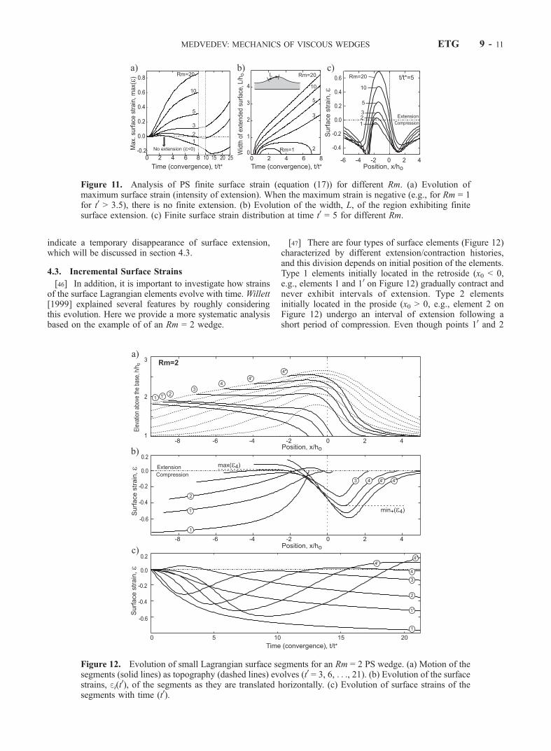
indicate a temporary disappearance of surface extension,which will be discussed in section 4.3.

4.3. Incremental Surface Strains

[46] In addition, it is important to investigate how strainsof the surface Lagrangian elements evolve with time. Willett[1999] explained several features by roughly consideringthis evolution. Here we provide a more systematic analysisbased on the example of of an Rm = 2 wedge.

[47] There are four types of surface elements (Figure 12)characterized by different extension/contraction histories,and this division depends on initial position of the elements.Type 1 elements initially located in the retroside (x0 < 0,e.g., elements 1 and 10 on Figure 12) gradually contract andnever exhibit intervals of extension. Type 2 elementsinitially located in the proside (x0 > 0, e.g., element 2 onFigure 12) undergo an interval of extension following ashort period of compression. Even though points 10 and 2

Figure 11. Analysis of PS finite surface strain (equation (17)) for different Rm. (a) Evolution ofmaximum surface strain (intensity of extension). When the maximum strain is negative (e.g., for Rm = 1for t0 > 3.5), there is no finite extension. (b) Evolution of the width, L, of the region exhibiting finitesurface extension. (c) Finite surface strain distribution at time t0 = 5 for different Rm.

Figure 12. Evolution of small Lagrangian surface segments for an Rm = 2 PS wedge. (a) Motion of thesegments (solid lines) as topography (dashed lines) evolves (t0 = 3, 6, . . ., 21). (b) Evolution of the surfacestrains, ei(t

0), of the segments as they are translated horizontally. (c) Evolution of surface strains of thesegments with time (t0).


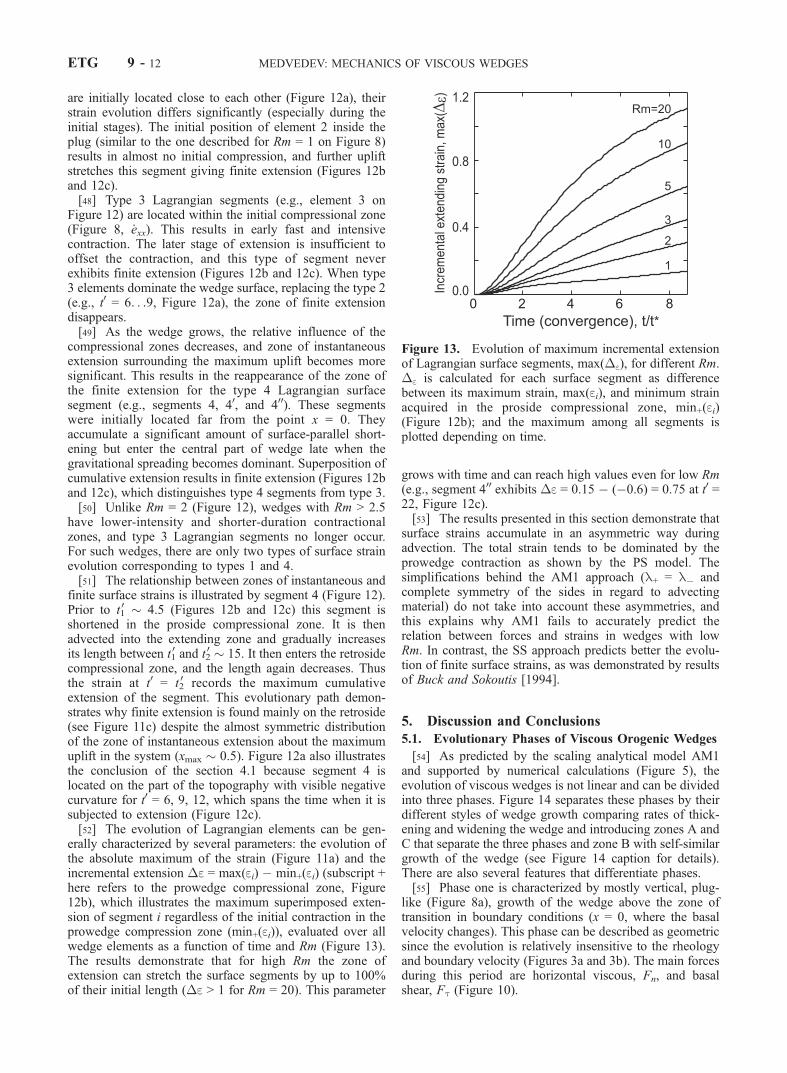
are initially located close to each other (Figure 12a), theirstrain evolution differs significantly (especially during theinitial stages). The initial position of element 2 inside theplug (similar to the one described for Rm = 1 on Figure 8)results in almost no initial compression, and further upliftstretches this segment giving finite extension (Figures 12band 12c).[48] Type 3 Lagrangian segments (e.g., element 3 on

Figure 12) are located within the initial compressional zone(Figure 8, _exx). This results in early fast and intensivecontraction. The later stage of extension is insufficient tooffset the contraction, and this type of segment neverexhibits finite extension (Figures 12b and 12c). When type3 elements dominate the wedge surface, replacing the type 2(e.g., t0 = 6. . .9, Figure 12a), the zone of finite extensiondisappears.[49] As the wedge grows, the relative influence of the

compressional zones decreases, and zone of instantaneousextension surrounding the maximum uplift becomes moresignificant. This results in the reappearance of the zone ofthe finite extension for the type 4 Lagrangian surfacesegment (e.g., segments 4, 40, and 400). These segmentswere initially located far from the point x = 0. Theyaccumulate a significant amount of surface-parallel short-ening but enter the central part of wedge late when thegravitational spreading becomes dominant. Superposition ofcumulative extension results in finite extension (Figures 12band 12c), which distinguishes type 4 segments from type 3.[50] Unlike Rm = 2 (Figure 12), wedges with Rm > 2.5

have lower-intensity and shorter-duration contractionalzones, and type 3 Lagrangian segments no longer occur.For such wedges, there are only two types of surface strainevolution corresponding to types 1 and 4.[51] The relationship between zones of instantaneous and

finite surface strains is illustrated by segment 4 (Figure 12).Prior to t 01 � 4.5 (Figures 12b and 12c) this segment isshortened in the proside compressional zone. It is thenadvected into the extending zone and gradually increasesits length between t 01 and t 02 � 15. It then enters the retrosidecompressional zone, and the length again decreases. Thusthe strain at t0 = t 02 records the maximum cumulativeextension of the segment. This evolutionary path demon-strates why finite extension is found mainly on the retroside(see Figure 11c) despite the almost symmetric distributionof the zone of instantaneous extension about the maximumuplift in the system (xmax � 0.5). Figure 12a also illustratesthe conclusion of the section 4.1 because segment 4 islocated on the part of the topography with visible negativecurvature for t0 = 6, 9, 12, which spans the time when it issubjected to extension (Figure 12c).[52] The evolution of Lagrangian elements can be gen-

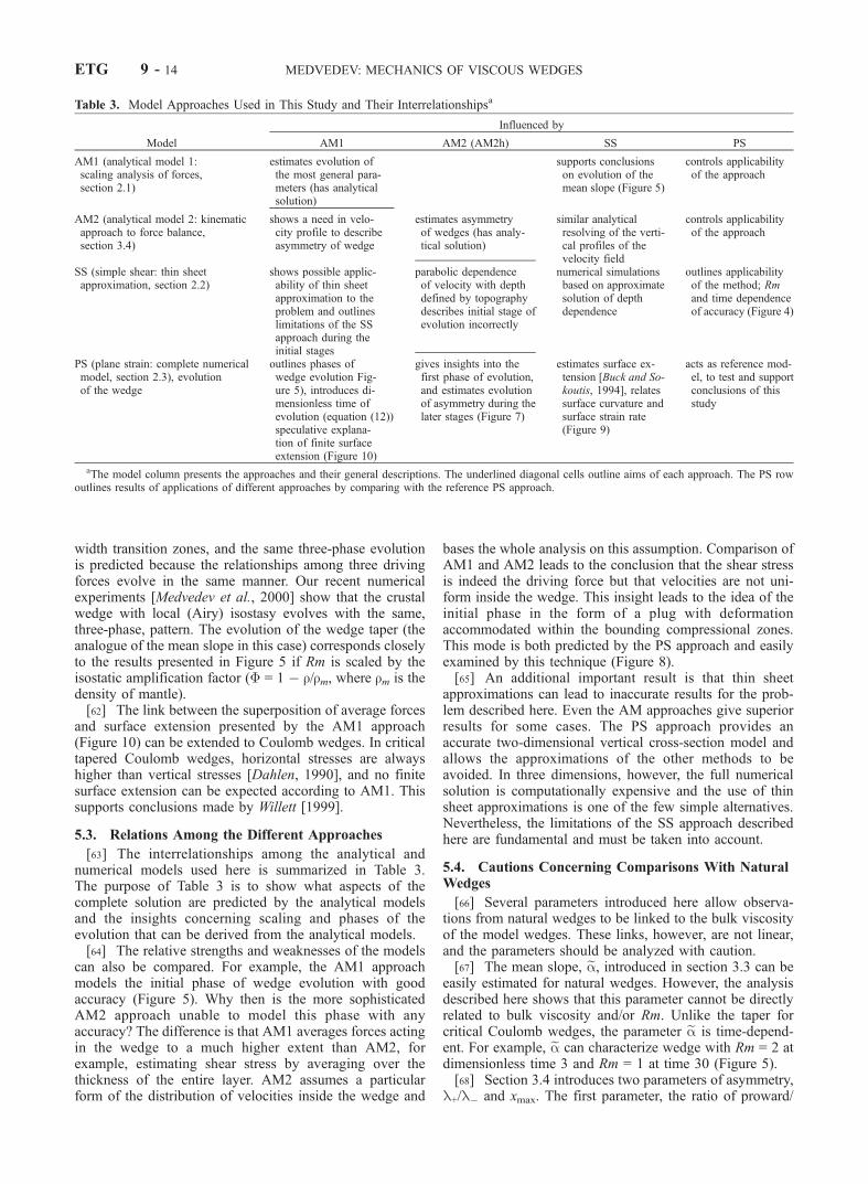
erally characterized by several parameters: the evolution ofthe absolute maximum of the strain (Figure 11a) and theincremental extension �e = max(ei) � min+(ei) (subscript +here refers to the prowedge compressional zone, Figure12b), which illustrates the maximum superimposed exten-sion of segment i regardless of the initial contraction in theprowedge compression zone (min+(ei)), evaluated over allwedge elements as a function of time and Rm (Figure 13).The results demonstrate that for high Rm the zone ofextension can stretch the surface segments by up to 100%of their initial length (�e > 1 for Rm = 20). This parameter

grows with time and can reach high values even for low Rm(e.g., segment 400 exhibits �e = 0.15 � (�0.6) = 0.75 at t0 =22, Figure 12c).[53] The results presented in this section demonstrate that

surface strains accumulate in an asymmetric way duringadvection. The total strain tends to be dominated by theprowedge contraction as shown by the PS model. Thesimplifications behind the AM1 approach (l+ = l� andcomplete symmetry of the sides in regard to advectingmaterial) do not take into account these asymmetries, andthis explains why AM1 fails to accurately predict therelation between forces and strains in wedges with lowRm. In contrast, the SS approach predicts better the evolu-tion of finite surface strains, as was demonstrated by resultsof Buck and Sokoutis [1994].

5. Discussion and Conclusions

5.1. Evolutionary Phases of Viscous Orogenic Wedges

[54] As predicted by the scaling analytical model AM1and supported by numerical calculations (Figure 5), theevolution of viscous wedges is not linear and can be dividedinto three phases. Figure 14 separates these phases by theirdifferent styles of wedge growth comparing rates of thick-ening and widening the wedge and introducing zones A andC that separate the three phases and zone B with self-similargrowth of the wedge (see Figure 14 caption for details).There are also several features that differentiate phases.[55] Phase one is characterized by mostly vertical, plug-

like (Figure 8a), growth of the wedge above the zone oftransition in boundary conditions (x = 0, where the basalvelocity changes). This phase can be described as geometricsince the evolution is relatively insensitive to the rheologyand boundary velocity (Figures 3a and 3b). The main forcesduring this period are horizontal viscous, Fn, and basalshear, Ft (Figure 10).

Figure 13. Evolution of maximum incremental extensionof Lagrangian surface segments, max(�e), for different Rm.�e is calculated for each surface segment as differencebetween its maximum strain, max(ei), and minimum strainacquired in the proside compressional zone, min+(ei)(Figure 12b); and the maximum among all segments isplotted depending on time.


[56] Phase two is transitional and is marked by a changein the orientation of preferred growth from vertical tohorizontal (with some period of close to self-similar growth,zone B on Figure 14) and by a change of the style ofasymmetry development (the separation point between twophases of asymmetry development estimated in section 3.4(Figure 7) is located in proximity to the zone B on Figure14). One of the main characteristics of this phase is theonset of finite surface extension The gravitational potentialenergy grows during the initial phase such that all threeforces described in the AM1 approach (equation (3))become important in phase 2 (Figure 10a).[57] Although the wedge grows continuously, the mean

slope of the wedge decreases during the third phase. Theinfluence of the normal horizontal viscous stress decreasesasymptotically during this phase, and the evolution is drivenby the equilibrium between gravitational spreading andshear traction along the base. By analogy with the modelof wedge evolution presented by Platt [1986], phase 3 canbe described as underthrusting (underplating).[58] Along with the dimensionless convergence time

(Table 1), the evolution time was introduced (equation(12)). The latter parameter includes rheological and boun-dary conditions of wedge evolution, and it demonstrates thescaling between the real time of evolution and the phases ofevolution (Figure 14). Equation (12) shows also that awedge evolves through these phases faster if it is charac-terized by relatively lower viscosity and/or higher conver-gence velocity and/or higher density.[59] Feehan and Brandon [1999] present a conceptual

model of different modes of steady state accretionry

wedges: ‘‘thickening’’ (described by mainly surface con-traction), ‘‘mixed,’’ and ‘‘thinning’’ (described by signifi-cant surface extension). The properties of these modes arelinked to the three phases presented here: the first phase ofwedge evolution is characterized by both rapid thickeningand surface compression; the third (final) stage is charac-terized mainly by widening of the wedge and broadeningthe zone of finite surface extension; the transition phase hasmixed characteristics of the two end phases. Thus the modesof steady state wedges described by Feehan and Brandon[1999] can be a result of reaching the stationary states atdifferent phases of wedge evolution.

5.2. Variations on the Simple Model

[60] The problem considered in this study is highlysimplified, and direct application of the results to tectonicwedges may be limited. However, analyzing the simplemodel can help to understand and even predict some resultsof variations of this model or more complicated models.[61] The boundary conditions used in this study to model

the wedge evolution include a discontinuity in basal veloc-ity at the point x = 0 (Figure 1a) or a corresponding rapidtransition in the PS models. This kind of boundary con-dition corresponds to asymmetric basal subduction orunderthrusting. Although it results in significant simplifica-tion of the analytical models, other boundary conditionsmay also prevail. We have also investigated several numer-ical PS models in which the basal boundary velocity is acontinuous function with broad transition. The results arequalitatively similar to those described earlier. Moreover,the AM1 approach can be extended to models with finite

Figure 14. Phases of viscous wedge growth demonstrated by the evolution of mean slope, ea (equation(11)). The three phases are I, initial, growth is mostly vertical; II, developed, growth is close to self-similar;and III, final, the wedge spreads horizontally. The size of arrows on bottom panels illustrates these relativestyles. These stages are separated by the asymptotic behavior of the growth of �h and l with time. Themass balance (equation (6)) relates these parameters and the convergence time as (�h

0 l0 = 2t0), which canbe rewritten as proportional relation (�h

0 l0 / t0). Thus, if growth of the maximum elevation scales withtime as (�h

0 / (t0)b), the deformations width scales as (l0 / (t)(1 � b)). During the initial phase,�h / t0 andb 1, while l const. Parameter b decreases with evolution of wedge. Zone A separates the first andsecond phases with the condition b 0.83. Zone B represents self-similar growth of the wedge withb 0.5 (note also that condition b = 0.5 is equivalent to condition of maximum mean slope). Zone Cindicates the onset of the third phase with b 0.4. In each of these zones (A, B, and C) the exact match tothe parameter value (b = 0.83, 0.5 and 0.4 correspondingly) is shown by the dashed line.


width transition zones, and the same three-phase evolutionis predicted because the relationships among three drivingforces evolve in the same manner. Our recent numericalexperiments [Medvedev et al., 2000] show that the crustalwedge with local (Airy) isostasy evolves with the same,three-phase, pattern. The evolution of the wedge taper (theanalogue of the mean slope in this case) corresponds closelyto the results presented in Figure 5 if Rm is scaled by theisostatic amplification factor (� = 1 � r/rm, where rm is thedensity of mantle).[62] The link between the superposition of average forces

and surface extension presented by the AM1 approach(Figure 10) can be extended to Coulomb wedges. In criticaltapered Coulomb wedges, horizontal stresses are alwayshigher than vertical stresses [Dahlen, 1990], and no finitesurface extension can be expected according to AM1. Thissupports conclusions made by Willett [1999].

5.3. Relations Among the Different Approaches

[63] The interrelationships among the analytical andnumerical models used here is summarized in Table 3.The purpose of Table 3 is to show what aspects of thecomplete solution are predicted by the analytical modelsand the insights concerning scaling and phases of theevolution that can be derived from the analytical models.[64] The relative strengths and weaknesses of the models

can also be compared. For example, the AM1 approachmodels the initial phase of wedge evolution with goodaccuracy (Figure 5). Why then is the more sophisticatedAM2 approach unable to model this phase with anyaccuracy? The difference is that AM1 averages forces actingin the wedge to a much higher extent than AM2, forexample, estimating shear stress by averaging over thethickness of the entire layer. AM2 assumes a particularform of the distribution of velocities inside the wedge and

bases the whole analysis on this assumption. Comparison ofAM1 and AM2 leads to the conclusion that the shear stressis indeed the driving force but that velocities are not uni-form inside the wedge. This insight leads to the idea of theinitial phase in the form of a plug with deformationaccommodated within the bounding compressional zones.This mode is both predicted by the PS approach and easilyexamined by this technique (Figure 8).[65] An additional important result is that thin sheet

approximations can lead to inaccurate results for the prob-lem described here. Even the AM approaches give superiorresults for some cases. The PS approach provides anaccurate two-dimensional vertical cross-section model andallows the approximations of the other methods to beavoided. In three dimensions, however, the full numericalsolution is computationally expensive and the use of thinsheet approximations is one of the few simple alternatives.Nevertheless, the limitations of the SS approach describedhere are fundamental and must be taken into account.

5.4. Cautions Concerning Comparisons With NaturalWedges

[66] Several parameters introduced here allow observa-tions from natural wedges to be linked to the bulk viscosityof the model wedges. These links, however, are not linear,and the parameters should be analyzed with caution.[67] The mean slope, ea, introduced in section 3.3 can be

easily estimated for natural wedges. However, the analysisdescribed here shows that this parameter cannot be directlyrelated to bulk viscosity and/or Rm. Unlike the taper forcritical Coulomb wedges, the parameter ea is time-depend-ent. For example, ea can characterize wedge with Rm = 2 atdimensionless time 3 and Rm = 1 at time 30 (Figure 5).[68] Section 3.4 introduces two parameters of asymmetry,

l+/l� and xmax. The first parameter, the ratio of proward/

Table 3. Model Approaches Used in This Study and Their Interrelationshipsa

Model

Influenced by

AM1 AM2 (AM2h) SS PS

AM1 (analytical model 1:scaling analysis of forces,section 2.1)

estimates evolution ofthe most general para-meters (has analyticalsolution)

supports conclusionson evolution of themean slope (Figure 5)

controls applicabilityof the approach

AM2 (analytical model 2: kinematicapproach to force balance,section 3.4)

shows a need in velo-city profile to describeasymmetry of wedge

estimates asymmetryof wedges (has analy-tical solution)

similar analyticalresolving of the verti-cal profiles of thevelocity field

controls applicabilityof the approach

SS (simple shear: thin sheetapproximation, section 2.2)

shows possible applic-ability of thin sheetapproximation to theproblem and outlineslimitations of the SSapproach during theinitial stages

parabolic dependenceof velocity with depthdefined by topographydescribes initial stage ofevolution incorrectly

numerical simulationsbased on approximatesolution of depthdependence

outlines applicabilityof the method; Rmand time dependenceof accuracy (Figure 4)

PS (plane strain: complete numericalmodel, section 2.3), evolutionof the wedge

outlines phases ofwedge evolution Fig-ure 5), introduces di-mensionless time ofevolution (equation (12))speculative explana-tion of finite surfaceextension (Figure 10)

gives insights into thefirst phase of evolution,and estimates evolutionof asymmetry during thelater stages (Figure 7)

estimates surface ex-tension [Buck and So-koutis, 1994], relatessurface curvature andsurface strain rate(Figure 9)

acts as reference mod-el, to test and supportconclusions of thisstudy

aThe model column presents the approaches and their general descriptions. The underlined diagonal cells outline aims of each approach. The PS rowoutlines results of applications of different approaches by comparing with the reference PS approach.


retroward length scales, shares properties of the mean slope:it can be directly estimated from topography of naturalorogens, and it is time-/phase-dependent. Figure 7a showsthat model wedges with different bulk rheologies can becharacterized by the same value of l+/l�.[69] The second asymmetry parameter, the shift of the

point of maximum uplift, xmax (Figure 7b), can be estimatedfrom the comparison of the topography with the seismicitydistribution in active orogens [e.g., Cahill and Isacks,1992]. Two characteristics of this parameter make it impor-tant: (1) after a short initial phase it reaches stable valuedirectly related to Rm; and (2) this parameter is a distinctcharacteristics of viscous wedges because frictional-brittlewedges result in xmax � 0 for wedges with the sameboundary conditions [Vanderhaeghe et al., 1998; Willett,1999].[70] The parameters of surface extension discussed in

section 4 can be compared with distribution of normal faultsoften observed along the natural wedges. The strain historyof surface segments considered in section 4.3 clearlyillustrates the zonation of surface strains in orogens. Thesepredictions can be tested by well-established methods ofstructural geology [e.g., Ramsay and Huber, 1983].[71] Although each parameter separately cannot provide

unique link between observations and the model, the set ofparameters presented can draw a clear picture of bulkrheology and dynamic conditions of natural wedges. Oncethe simple model described here becomes clear, morecomplicated models can be built and tested using the similarpattern of descriptive parameters.

[72] Acknowledgments. This work would be impossible withoutgenerous help from other members of Dalhousie Geodynamics Group:Chris Beaumont suggested the problem and significantly improved thepresentation and structure of the manuscript; Olivier Vanderhaeghe sug-gested several topics for consideration; Philippe Fullsack provided his codeand helped with the PS approach. This collaboration allows me to use ‘‘we’’throughout the paper, although any of the errors are mine only. Commentsby Djordje Grujic and two anonymous reviewers were helpful. ThomasFunck is thanked for help in preparation of figures. Research was funded byan NSERC research grant to C. Beaumont.

ReferencesBeaumont, C., P. Fullsack, and J. Hamilton, Styles of crustal deformationcaused by subduction of the underlying mantle, Tectonophysics, 232,119–132, 1994.

Beaumont, C., P. J. J. Kamp, J. Hamilton, and P. Fullsack, The continentalcollision zone, South Island, New Zealand: Comparison of geodynamicalmodels and observations, J. Geophys. Res., 101, 3333–3359, 1996.

Beaumont, C., J. A. Munoz, J. Hamilton, and P. Fullsack, Factors control-ling the Alpine evolution of the central Pyrenees inferred from a compar-ison of observation and geodynamical models, J. Geophys. Res., 105,8121–8145, 2000.

Buck, W. R., and D. Sokoutis, Analogue model of gravitational collapseand surface extension during continental convergence, Nature, 369, 737–740, 1994.

Cahill, T., and B. L. Isacks, Seismicity and shape of the subducted NazcaPlate, J. Geophys. Res., 97, 17,503–17,529, 1992.

Cuvelier, C., A. Segal, and A. A. Steenhoven, Finite Element Methods andNavier-Stokes Equations, 483 pp., D. Reidel, Norwell, Mass., 1986.

Dahlen, F. A., Critical taper model of fold-and-thrust belts and accretionarywedges, Annu. Rev. Earth Planet. Sci., 18, 55–99, 1990.

Ellis, S., Forces driving continental collision: Reconciling indentation andmantle subduction tectonics, Geology, 24, 699–702, 1996.

Ellis, S., P. Fullsack, and C. Beaumont, Oblique convergence of thecrust driven by basal forcing: Implication for length-scales of deforma-tion and strain partitioning in orogens, Geophys. J. Int., 120, 24–44,1995.

Ellis, S., C. Beaumont, R. Jamieson, and G. Quinlan, Continental collisionincluding a weak zone—The vise model and its application to the New-foundland Appalachians, Can. J. Earth Sci., 35, 1323–1346, 1998.

Emerman, S. H., and D. L. Turcotte, A fluid model for the shape of accre-tionary wedges, Earth Planet. Sci. Lett., 63, 379–384, 1983.

England, P., and D. McKenzie, A thin viscous sheet model for continentaldeformation, Geophys. J. R. Astron. Soc., 70, 295–321, 1982.

Feehan, J., and M. Brandon, Contribution of ductile flow to exhumation ofa thrust wedge, San Juan –Cascade nappes, NW Washington State,J. Geophys. Res., 104, 10,883–10,902, 1999.

Fullsack, P., An arbitrary Lagrangian-Eulerian formulation for creepingflows and applications in tectonic models, Geophys. J. Int., 120, 1–23,1995.

Jones, C. H., J. R. Unrih, and L. J. Sonder, The role of gravitationalpotential energy in active deformation in the southwestern United States,Nature, 381, 37–41, 1996.

Lobkovsky, L. I., and V. I. Kerchman, A two-level concept of plate tectonics:Application to geodynamics, Tectonophysics, 199, 343–374, 1991.

Medvedev, S. E., Computer simulation of sedimentary cover evolution, inComputerized Basin Analysis: The Prognosis of energy and MineralResources, edited by J. Harff and D. F. Merriam, pp. 1–10, Plenum,New York, 1993.

Medvedev, S. E., and Y. Y. Podladchikov, New extended thin sheet approx-imation for geodynamic applications I, Model formulation, Geophys.J. Int., 136, 567–585, 1999a.

Medvedev, S. E., and Y. Y. Podladchikov, New extended thin sheet approx-imation for geodynamic applications, II, 2D examples, Geophys. J. Int.,136, 586–608, 1999b.

Medvedev, S., C. Beaumont, O. Vanderhaeghe, P. Fullsack, and R. A.Jamieson, Evolution of continental plateaus: Insights from thermal-me-chanical modeling (abstract), Eos Trans. AGU, 81(48), Fall Meet. Suppl.,Abstract T52B-17, 2000.

Petrini, K., and Y. Podladchikov, Lithospheric pressure-depth relationshipin compressive regions of thickened crust, J. Metamorph. Geol., 18, 67–78, 2000.

Platt, J. P., Dynamics of orogenic wedges and the uplift of high-pressuremetamotphic rocks, Geol. Soc. Am. Bull., 97, 1037–1053, 1986.

Platt, J. P., Mechanics of oblique convergence, J. Geophys. Res., 98,16,232–16,256, 1993.

Platt, J. P., Calibrating the bulk rheology of active obliquely convergentthrust belts and forearc wedges from surface profiles and velocity dis-tributions, Tectonics, 19, 529–548, 2000.

Ramberg, H., Gravity, Deformation and the Earth’s Crust, 2nd ed., 452 p.,Academic, San Diego, Calif., 1981.

Ramsay, J. G., and M. I. Huber, The Techniques of Modern StructuralGeology, vol. 1, Strain Analysis, 307 pp., Academic, San Diego, Calif.,1983.

Ring, U., M. T. Brandon, Ductile strain, coaxial deformation and mass lossin the Franciscan complex: Implications for exhumation processes insubduction zones, in Exhumation Processes: Normal Faulting, DuctileFlow and Erosion, edited by U. Ring et al., Geol. Soc. Spec. Publ., 154,55–86, 1999

Royden, L., Coupling and decoupling of crust and mantle in convergentorogens: Implications for strain partitioning in the crust, J. Geophys. Res.,101, 17,679–17,705, 1996.

Schlichting, G., Boundary-Layer Theory, 7th ed., McGraw-Hill, New York,1979.

Shen, F., L. H. Royden, and B. B. Clark, Large-scale crustal deformation ofthe Tibetan Plateau, J. Geophys. Res., 106, 6793–6816, 2001.

Vanderhaeghe, O., C. Beaumont, P. Fullsack, S. Medvedev, and R. A.Jamieson, Thermal-mechanical modelling of convergent orogens: Therole of rheology, isostasy and temperature, in ECSOOT 73rd TransectMeeting, edited by R. Wardle and J. Hall, 44–85, Lithoprobe Secretariat,Vancouver, B. C., Canada, 1998.

Weijemars, R., and H. Schmeling, Scaling of newtonian and non newtonianfluid dynamics without inertia for quantative modelling of rock flow dueto gravity (including the concept of rheological similarity), Phys. EarthPlanet. Inter., 43, 938–954, 1986.

Willett, S. D., Rheological dependence of extension in wedge models ofconvergent orogens, Tectonophysics, 305, 419–435, 1999.

Zanemonetz, V. B., V. O. Mikhajlov, and V. P. Myasnikov, Mechanicalmodel of block folding formation, Phys. Solid Earth, 12, 631–635, 1976.

Zienkiewicz, O. C., and R. L. Taylor, The Finite Element Method, 4th ed.,1400 pp., McGraw-Hill, New York, 1989.

��S. Medvedev, Department of Oceanography, Dalhousie University,

Halifax, Nova Scotia, Canada B3H 4J1. ([email protected])


Mechanics of viscous wedges: Modeling by analytical and ...

Documents

Transcript of Mechanics of viscous wedges: Modeling by analytical and ...