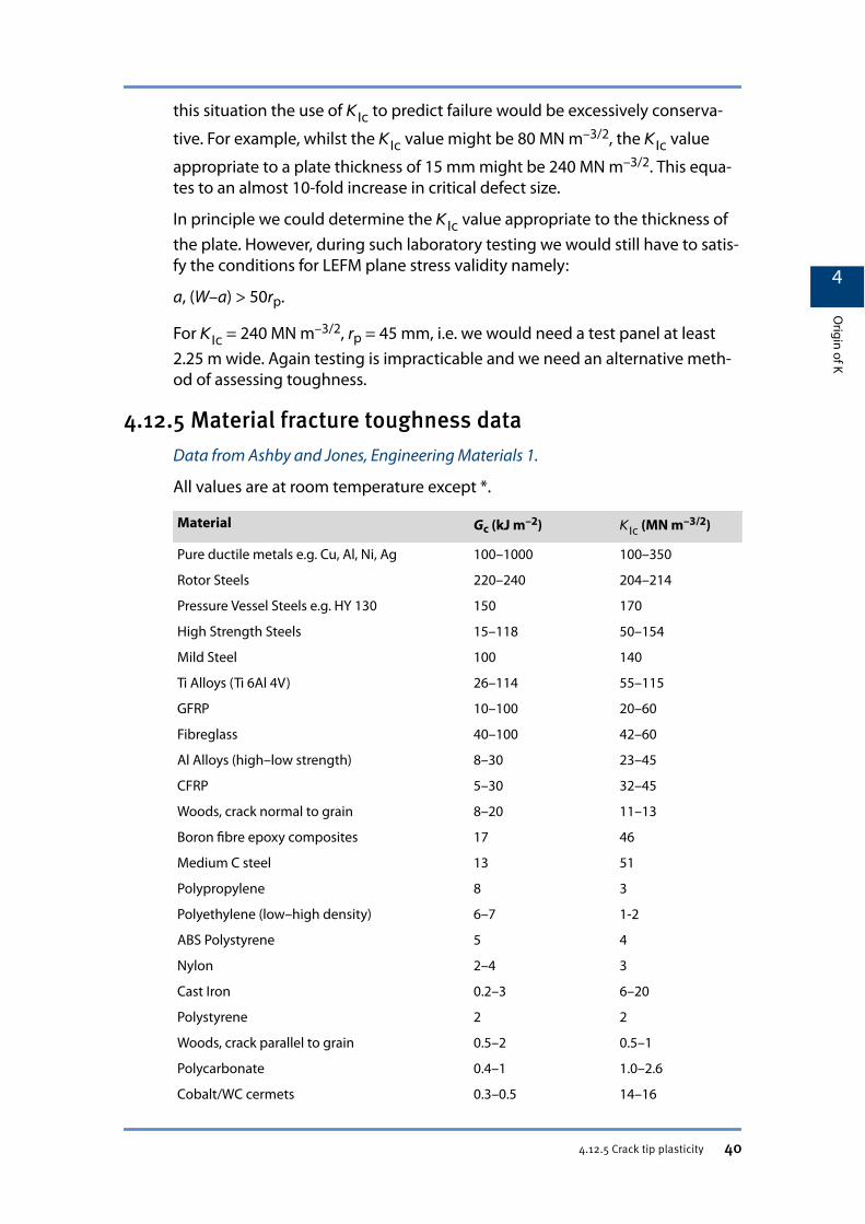
Mechanics ME3 Fundamentals of Fracture - Dr. Brian...
86
ME3 Fundamentals of Fracture Mechanics Lecture notes 2014-15 Shaun Crofton Imperial College London UK
Transcript of Mechanics ME3 Fundamentals of Fracture - Dr. Brian...
ME3 Fundamentals of Fracture Mechanics
Lecture notes 2014-15
Shaun CroftonImperial College London
UK
Introduction● Aims
1. To develop an understanding of the various aspects involved in the areaof fracture mechanics.
2. To develop from first principles the basic ideas and equations needed foran understanding of fracture mechanics
3. To define the advantages and disadvantages of this approach for study-ing the failure of materials and structures.
4. To indicate how the basic principles may be applied to a range of industri-al problems and materials.
5. To lay foundations for the ME4 Advanced Forming and Fracture course.
● Recommended background reading
1. TL Anderson, Fracture Mechanics — Fundamentals and Applications (3rded.). Taylor and Francis (2012),
2. D Broek, Elementary Fracture Mechanics. Martinus Nijhoff (1987).
3. AJ Kinloch and RJ Young, Fracture Behavious of Polymers. Elsevier (1983).
4. JG Williams, Fracture Mechanics of Polymers. Ellis Horwood (1984).
5. D Hull, An Introduction to Composite Materials. Cambridge University Press(1981).
6. FL Matthews and RD Rawlings, Composite Materials: Engineering and Sci-ence. Chapman and Hall (1994).
RELATED LINKS
Link to PDF of TL Anderson, "Fracture Mechanics".
i
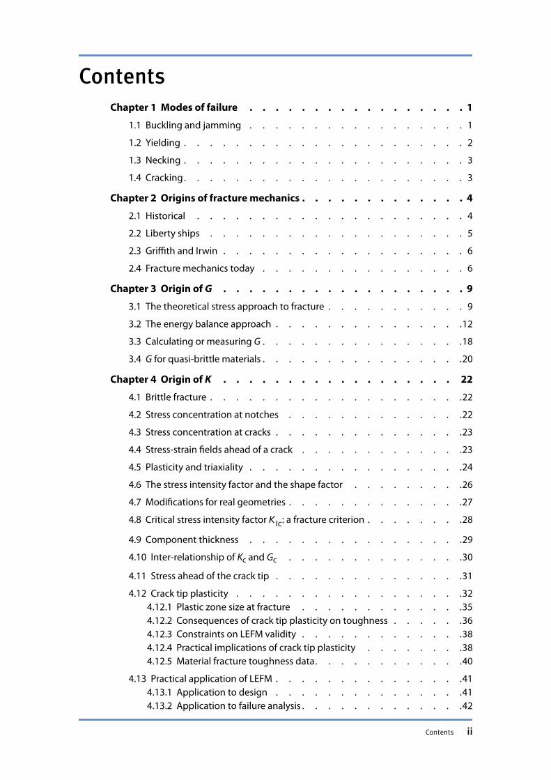
ContentsChapter 1 Modes of failure . . . . . . . . . . . . . . . . . 1
1.1 Buckling and jamming . . . . . . . . . . . . . . . . . 1
1.2 Yielding . . . . . . . . . . . . . . . . . . . . . . 2
1.3 Necking . . . . . . . . . . . . . . . . . . . . . . 3
1.4 Cracking. . . . . . . . . . . . . . . . . . . . . . 3
Chapter 2 Origins of fracture mechanics . . . . . . . . . . . . . 4
2.1 Historical . . . . . . . . . . . . . . . . . . . . . 4
2.2 Liberty ships . . . . . . . . . . . . . . . . . . . . 5
2.3 Griffith and Irwin . . . . . . . . . . . . . . . . . . . 6
2.4 Fracture mechanics today . . . . . . . . . . . . . . . . 6
Chapter 3 Origin of G . . . . . . . . . . . . . . . . . . . 9
3.1 The theoretical stress approach to fracture . . . . . . . . . . . 9
3.2 The energy balance approach . . . . . . . . . . . . . . .12
3.3 Calculating or measuring G . . . . . . . . . . . . . . . .18
3.4 G for quasi-brittle materials . . . . . . . . . . . . . . . .20
Chapter 4 Origin of K . . . . . . . . . . . . . . . . . . 22
4.1 Brittle fracture . . . . . . . . . . . . . . . . . . . .22
4.2 Stress concentration at notches . . . . . . . . . . . . . .22
4.3 Stress concentration at cracks . . . . . . . . . . . . . . .23
4.4 Stress-strain fields ahead of a crack . . . . . . . . . . . . .23
4.5 Plasticity and triaxiality . . . . . . . . . . . . . . . . .24
4.6 The stress intensity factor and the shape factor . . . . . . . . .26
4.7 Modifications for real geometries . . . . . . . . . . . . . .27
4.8 Critical stress intensity factor KIc: a fracture criterion . . . . . . . .28
4.9 Component thickness . . . . . . . . . . . . . . . . .29
4.10 Inter-relationship of Kc and Gc . . . . . . . . . . . . . .30
4.11 Stress ahead of the crack tip . . . . . . . . . . . . . . .31
4.12 Crack tip plasticity . . . . . . . . . . . . . . . . . .324.12.1 Plastic zone size at fracture . . . . . . . . . . . . .354.12.2 Consequences of crack tip plasticity on toughness . . . . . .364.12.3 Constraints on LEFM validity . . . . . . . . . . . . .384.12.4 Practical implications of crack tip plasticity . . . . . . . .384.12.5 Material fracture toughness data. . . . . . . . . . . .40
4.13 Practical application of LEFM . . . . . . . . . . . . . . .414.13.1 Application to design . . . . . . . . . . . . . . .414.13.2 Application to failure analysis . . . . . . . . . . . . .42
Contents ii
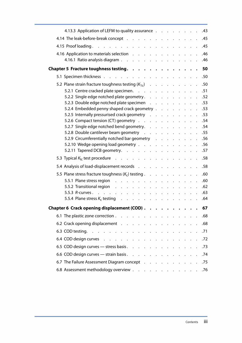
4.13.3 Application of LEFM to quality assurance . . . . . . . . .43
4.14 The leak-before-break concept . . . . . . . . . . . . . .45
4.15 Proof loading . . . . . . . . . . . . . . . . . . . .45
4.16 Application to materials selection . . . . . . . . . . . . .464.16.1 Ratio analysis diagram . . . . . . . . . . . . . . .46
Chapter 5 Fracture toughness testing. . . . . . . . . . . . . 50
5.1 Specimen thickness . . . . . . . . . . . . . . . . . .50
5.2 Plane strain fracture toughness testing (K1c) . . . . . . . . . .505.2.1 Centre cracked plate specimen. . . . . . . . . . . . .515.2.2 Single edge notched plate geometry . . . . . . . . . . .525.2.3 Double edge notched plate specimen . . . . . . . . . .535.2.4 Embedded penny shaped crack geometry . . . . . . . . .535.2.5 Internally pressurised crack geometry . . . . . . . . . .535.2.6 Compact tension (CT) geometry . . . . . . . . . . . .545.2.7 Single edge notched bend geometry. . . . . . . . . . .545.2.8 Double cantilever beam geometry . . . . . . . . . . .555.2.9 Circumferentially notched bar geometry . . . . . . . . .565.2.10 Wedge opening load geometry . . . . . . . . . . . .565.2.11 Tapered DCB geometry. . . . . . . . . . . . . . .57
5.3 Typical KIc test procedure . . . . . . . . . . . . . . . .58
5.4 Analysis of load-displacement records . . . . . . . . . . . .58
5.5 Plane stress fracture toughness (Kc) testing . . . . . . . . . . .605.5.1 Plane stress region . . . . . . . . . . . . . . . .605.5.2 Transitional region . . . . . . . . . . . . . . . .625.5.3 R-curves . . . . . . . . . . . . . . . . . . . .635.5.4 Plane stress Kc testing . . . . . . . . . . . . . . .64
Chapter 6 Crack opening displacement (COD) . . . . . . . . . . 67
6.1 The plastic zone correction . . . . . . . . . . . . . . . .68
6.2 Crack opening displacement . . . . . . . . . . . . . . .68
6.3 COD testing. . . . . . . . . . . . . . . . . . . . .71
6.4 COD design curves . . . . . . . . . . . . . . . . . .72
6.5 COD design curves — stress basis . . . . . . . . . . . . . .73
6.6 COD design curves — strain basis . . . . . . . . . . . . . .74
6.7 The Failure Assessment Diagram concept . . . . . . . . . . .75
6.8 Assessment methodology overview . . . . . . . . . . . . .76
Contents iii
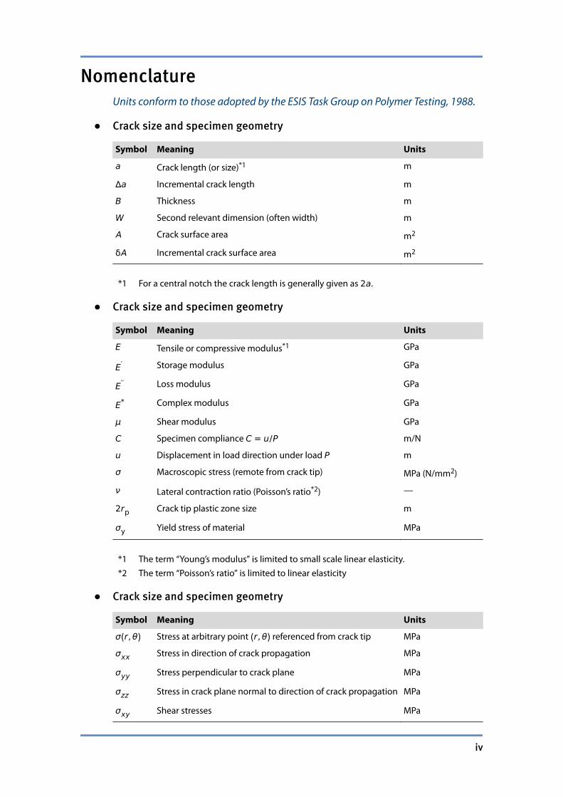
NomenclatureUnits conform to those adopted by the ESIS Task Group on Polymer Testing, 1988.
● Crack size and specimen geometry
Symbol Meaning Units
a Crack length (or size)*1 m
Δa Incremental crack length m
B Thickness m
W Second relevant dimension (often width) m
A Crack surface area m2
δA Incremental crack surface area m2
*1 For a central notch the crack length is generally given as 2a.
● Crack size and specimen geometry
Symbol Meaning Units
E Tensile or compressive modulus*1 GPa
E′ Storage modulus GPa
E′′ Loss modulus GPa
E* Complex modulus GPa
μ Shear modulus GPa
C Specimen compliance C = u/P m/N
u Displacement in load direction under load P m
σ Macroscopic stress (remote from crack tip) MPa (N/mm2)
ν Lateral contraction ratio (Poisson’s ratio*2) —
2rp Crack tip plastic zone size m
σy Yield stress of material MPa
*1 The term “Young’s modulus” is limited to small scale linear elasticity.*2 The term “Poisson’s ratio” is limited to linear elasticity
● Crack size and specimen geometry
Symbol Meaning Units
σ r,θ Stress at arbitrary point r,θ referenced from crack tip MPa
σxx Stress in direction of crack propagation MPa
σyy Stress perpendicular to crack plane MPa
σzz Stress in crack plane normal to direction of crack propagation MPa
σxy Shear stresses MPa
iv
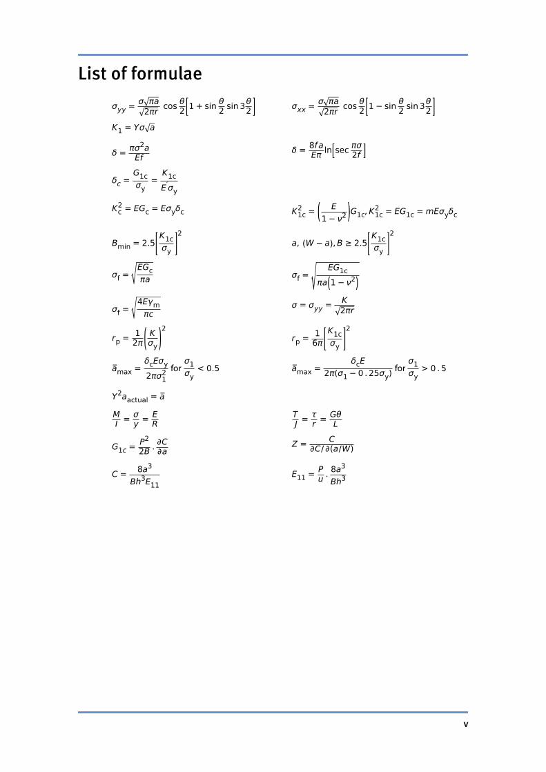
List of formulae
σyy = σ πa2πr cos θ2 1 + sin θ2 sin 3θ2 σxx = σ πa
2πr cos θ2 1− sin θ2 sin 3θ2
K1 = Yσ a
δ = πσ2aEf
δ = 8faEπ ln sec πσ2f
δc =G1cσy
=K1cE′σy
Kc2 = EGc = Eσyδc K1c
2 = E1− ν2 G1c, K1c
2 = EG1c =mEσyδc
Bmin = 2.5K1cσy
2a, W − a ,B ≥ 2.5
K1cσy
2
σf =EGcπa σf =
EG1cπa 1− ν2
σf =4Eγmπc
σ = σyy = K2πr
rp = 12π
Kσy
2rp = 1
6πK1cσy
2
amax =δcEσy2πσ1
2 for σ1σy
< 0.5 amax =δcE
2π(σ1− 0 . 25σy) for σ1σy
> 0 . 5
Y2aactual = a
MI = σ
y = ER
TJ = τ
r = GθL
G1c = P22B . ∂C∂a
Z = C∂C/ ∂(a/W)
C = 8a3
Bh3E11E11 = P
u . 8a3
Bh3
v
Chapter 1 Modes of failureGetting fracture in perspective, as one amongst several distinct failure modes forengineering structures.
Engineering design methodology requires that the designer should be awareof the possible modes of failure of a component or structure, so that the de-sign process can be carried out with a view to ensuring the avoidance of allpossible, relevant, failure modes. In some respects, one of the major skills indesigning is being able to correctly identify the most probable failure mecha-nism. Almost all the classic failure stories from industry relate to machines orobjects where the designer got it wrong, sometimes with tragic consequen-ces.
A classification of the more common failure modes known for structural com-ponents can be made as follows:
• Failure by elastic instability (buckling);
• Failure by excessively large elastic deformations (jamming);
• Failure by gross plastic deformation (yielding);
• Failure by tensile instability (necking);
• Failure by fast fracture (cracking, snapping);
• Failure by environmental corrosion (rusting, rotting).
This course aims to demonstrate and explain the techniques available for ‘de-signing against fracture’. However, a brief study of each one of the failuremodes listed above is given for the following purposes:
1. To put fracture mechanics into context for the design engineer, and
2. To provide some background information on how the development ofmaterials which exhibit good performance in terms of resistance to fail-ure by yielding, effectively encouraged a relatively new type of failure: bycracking.
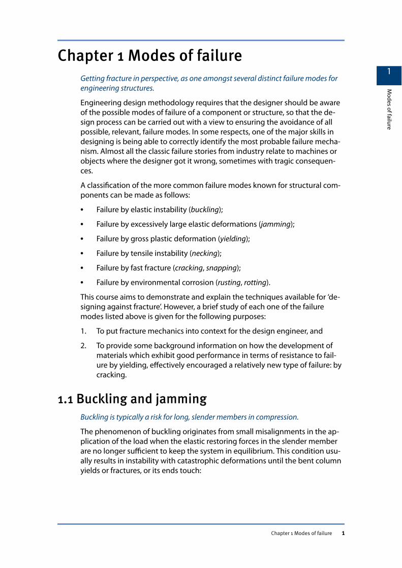
1.1 Buckling and jammingBuckling is typically a risk for long, slender members in compression.
The phenomenon of buckling originates from small misalignments in the ap-plication of the load when the elastic restoring forces in the slender memberare no longer sufficient to keep the system in equilibrium. This condition usu-ally results in instability with catastrophic deformations until the bent columnyields or fractures, or its ends touch:
1
Modes of failure
Chapter 1 Modes of failure 1
Jamming can occur when, as a result of an oversight in design, excessivelylarge elastic deflections take place. It is a risk in the design of engines, for ex-ample, when clearances between components are very small.
Avoidance of both types of failure can be ensured by geometric specifications.
Currently much research is being carried out on the development of highmodulus materials, often containing fibres, to allow high stresses to be ap-plied without the development of high strain values. The reality is that in prac-tice, the available ratios of Young’s Modulus to density (E/ρ) do not offer thedesign engineer a broad spectrum from which to choose.
1.2 YieldingThe engineer understands this term to mean both localised yielding and failure byplastic collapse.
A failure by yielding can occur with general yielding or with the onset of limi-ted plastic deformation in the component in question.
From Knott Fundamentals of Fracture Mechanics:
“A body is said to have undergone general yielding when it is no longer possible totrace a path, across the load bearing section, through elastically deformed materi-al only.”
In the past, design would invariably aim to avoid the onset of any yielding.Current design methods can use localised yielding or plastic collapse as thelimiting criteria in a certain design situations.
Plastic collapse can be used as a safety feature in emergency situations, for ex-ample, in the choice of Armco crash barriers for use as the central reservationof a motorway or around race tracks: large plastic deformation of the barrier isdesirable so that the large forces experienced in an accident can be absorbedwith less risk to the drivers.
Plastic deformation can also be desired and induced in certain situations in or-der to create beneficial residual stresses or to blunt sharp defects.
Examples:
• autofrettaging of tubes;
1
Modes of failure
1.2 Yielding 2
• proof testing of pressure vessels beyond yielding.
In the design against failure by plastic collapse, the engineer is no longer re-stricted to a range of geometries or a limited choice of elastic constants. Awide choice of materials with various yield strengths is available.
RELATED LINKS
Example of Armco barrier installation
1.3 NeckingA risk for tension members subjected to a soft (load-controlled) loading.
Necking can only happen as a result of a gross overload and depends on theinteraction of material properties with the structure’s geometry and the ap-plied stress system.
Assuming that problems with buckling/jamming and necking can be preven-ted by design of the structural member and by limiting tensile stresses thenthe failure mode to guard against is yielding.
In order to design against necking failures, design codes have been developedand the application of safety factors ensures that necking failure is highly un-likely. However, the economic imperative of the last fifty years has led to at-tempts to use higher stresses for a given geometrical configuration requiringmaterials of higher uniaxial strength. The development of these high strengthmaterials and their efficient usage has rendered structures prone to failure byan alternative mode of failure: namely fast fracture or cracking.
1.4 CrackingProgressive separation of a structure into two pieces by the creation of new sur-face area.
Fast fracture is the unstable propagation of a crack in a structure and is almostinvariably produced by applied stresses apparently less than the design stresscalculated with the appropriate design code. The resulting catastrophic natureof these failures led to the development of Fracture Mechanics. These failureswere often described by the term brittle, applied in the macro sense ratherthan as a description of the micromechanisms of crack extension.
A brittle fracture is one in which the onset of unstable crack propagation isproduced by an applied stress less than the general yield stress of the un-cracked ligament remaining when instability first occurs.
These failures are usually associated with gross stress concentrations in largecomponents or structures and with loading systems which don’t relax the ap-plied stresses as the crack extends. Although in steels these fractures happenat low temperatures and/or in thick sections, for both aluminium and steelthey can also take place in very thin sheets.
1
Modes of failure
1.3 Necking 3
Chapter 2 Origins of fracture mechanicsAn account of how and why fracture mechanics emerged as a distinct discipline.
Why do materials fracture ?
To try to answer this question we need to start by answering the more funda-mental question for engineers and society at large — why should we be con-cerned about fracture ?
The answer is hopefully obvious, and intuitively it seems that society was al-ways concerned with fracture.
2.1 HistoricalPreviously exploited to shape hard, strong, natural materials, fracture later be-came a problem for more ductile materials.
In the Stone Age man used a variety of materials as well as stone. Some of thefirst craftsmen to engage in series production of useful items were the flintaxehead makers and they appreciated that flint was a hard, relatively strongbut under some circumstances hopelessly brittle material. Flint axeheadscould be shaped by fracturing flint or other stones to give the rough outlineshape required and this was normally accomplished by judicious hammeringagainst another stone to cause the axehead to fracture along planes of weak-ness.
Useful though they were for crushing the heads of the odd sabre tooth tigerthe flint axehead has a nasty tendency to shatter when struck against theground or rocks — not a very useful property !
Bronze age man improved things no end by developing a material capable ofbeing moulded to virtually any form and possessing the wondrous property ofbeing ductile. However bronze is, if anything, too soft to make good cuttingtools or weapons.
With the dawn of the Iron Age and ensuing centuries the artisans who werethe precursors of the modern day engineer really had a material which pos-sessed a good balance of strength and hardness but still a material with an an-noying propensity to fracture unexpectedly.
Since approximately the beginning of this century engineers plus the oddmetallurgist and physicist have been trying to answer the question “how do Istop it breaking or fracturing?”
The first approach was one still in common usage today. Because nobody real-ly appreciated the mechanism by which materials fractured the approach tak-en was to overdesign the component by accepting the brittle nature of thematerial of construction and limiting the stress on the component to some
2
Origins of fracture m
echanics
Chapter 2 Origins of fracture mechanics 4
small fraction of the tensile strength. At the same time it became common-place to proof test structures and components by subjecting them to a muchlarger load or stress than they would see in service.
Early cannons and muskets were proof tested by inserting an extra largecharge (double or treble charge of gunpowder) and firing the piece. If the gunsurvived in one piece then the chances were very good that it would survive inservice for a reasonable period of time. The bascules of Tower Bridge wereproof tested by parking horse drawn carts filled with large iron weights allover the bridge decking until it was deemed that the load was double thatwhich might be experienced in reality. The recent centenary of Tower Bridgewould indicate that this design philosophy has some merit. The bill for theconstruction of Tower Bridge on the other hand demonstrates the inadequacyof this approach. Safety factors approaching 10 on yield or tensile strength donot make for a cheap construction! Despite this design philosophy and thegenerally low applied stresses utilised, catastrophic fractures continued to oc-cur from time to time in a wide variety of components and structures. Steamboilers and railway equipment were particularly troublesome!
2.2 Liberty shipsA single, notorious case which motivated the modern study of fracture.
It was not until the 1940s when a series of catastrophic failures of steel struc-tures gave sufficient impetus that attention was turned to attempting to an-swer the far more fundamental questions of “why and how does it break?”.
As part of the wartime Lend-Lease agreement between the US and UK it be-came obvious that the UK did not have enough commercial shipping capacityto be able to transport the quantities of materiel required from the US to UKports. Additionally one of our European neighbours was deliberately fractur-ing our ships faster than we could build them. The US government thereforecalled for tenders to build a large number of general purpose cargo ships andtankers with the express purpose of transporting weapons, food and oil fromthe Eastern seaboard of the US to the UK. The tender required that these ves-sels should be built in a matter of a few months rather the years required byconventional riveted plate construction. The majority of N. American shipyardssaid it was impossible but a Californian civil engineer, curiously enough calledKaiser, claimed that he could meet the deadlines using a novel constructionmethod of a ship assembly line and all welded construction. The history ofthese so-called ‘Liberty’ ships is well known. Suffice it to say that of the ~2500ships built, over 140 broke in two and nearly 700 suffered serious crackingproblems, some when lying in port but invariably in cold weather.
At the end of the second world war a commission was set up to try to answerthe question as to why these ships had failed. Tests on plates from the frac-tured ships showed that in order not to fail by catastrophic cleavage fracturethe ships plate had to have a minimum value of Charpy Energy of about 35 J at0°C and exhibit less than 70% crystallinity. It was further determined that all
2
Origins of fracture m
echanics
2.2 Liberty ships 5
the serious cracking was by brittle fracture from either preexistent flaws orstress concentrations in steel plates which did not meet this criterion.
2.3 Griffith and IrwinTwo 20th century researchers on whose work the modern subject of Fracture Me-chanics is constructed.
A far more fundamental piece of research had already been carried out by A.A.Griffiths, a British physicist who, in 1920, had addressed the problem of whyglass fibres fracture at stress levels approximately two orders of magnitudebelow their theoretical strength. Griffiths recognised that the separation ofglass is a fracture dominated process in which fracture is inevitable if the ex-tension of an existing crack lowers the overall energy of the system. This appa-rently very simple concept is an example of an energy balance (thermodynam-ic) approach to fracture in which the decrease in elastic strain energy of thecracked body is counteracted by the energy needed or required to create thetwo new crack surfaces.
The major advance on this earlier theory was due to G.R. Irwin, who in the late1940s pointed out that to apply a Griffith criterion to the fracture of metallicmaterials required that instead of considering the energy balance as being be-tween the strain energy of the body and the surface energy term, as is thecase for a truly brittle material like glass, the energy balance for a metallic ma-terial should be between the elastic strain energy and the surface energy plusthe work done in plastic deformation. Most importantly Irwin also recognisedthat for a metallic material the work done in producing the plastic deforma-tion is invariably orders of magnitude greater than the surface energy term.
Thus the basis for fracture mechanics came about with the definition of a ma-terial property G which is defined as the total energy absorbed during a unitincrement of crack length per unit thickness. Nowadays G is invariably referredto as the strain energy release rate.
Only a few years later Irwin made a further fundamental step by showing thatit was possible to reconcile the concept of a critical stress intensity causingfracture, Kc, with the idea of a critical value of the strain energy release rate,Gc. The realisation that the strain energy and stress intensity approaches tothe prediction of fracture are equivalent led to a rapid development in the dis-cipline of Linear Elastic Fracture Mechanics (LEFM) which allows engineers topredict what defects are tolerable in a given structure under known loadingconditions — the basic goal of Fracture Mechanics.
2.4 Fracture mechanics todayThe analysis and prediction of fracture steadily improve, but materials are loadedever closer to their strength limits.
Curiously enough, as our knowledge of fracture mechanics has improved thenumber of catastrophic fracture incidents has continued to increase in
2
Origins of fracture m
echanics
2.3 Griffith and Irwin 6
absolute terms. However, we are becoming very good at explaining the causeof such catastrophic fractures, albeit after the event. A major reason for this isquite simply the increased usage of high performance materials (HS steels, HSAl alloys, titanium alloys, ceramics etc.) which are more fracture susceptible aswe will see later. A secondary reason may well be due to the fact that the in-creasing complexity of modern structures and machines renders exhaustiveanalysis of all possible loading configurations very difficult and time consum-ing.
This apparent lack of success should not be taken as an indictment of the in-adequacy of our understanding of the causes of fracture events. Brittle frac-ture is sometimes potentiated by financial imperative which drives manufac-turers to try to improve margins by “extending” the operating service enve-lope of components to the extent that intrinsic safety factors become compro-mised in the extreme event. Too often when a major component or structurefails in such a catastrophic manner it becomes apparent during the post mor-tem design review that the original component or structure was not designedusing any form of fracture assessment or prediction techniques.
Despite nearly fifty years of research and development it is a sad fact of lifethat the application and practice of fracture mechanics analysis techniques isstill generally confined to large sophisticated organisations such as aerospacecompanies and bridge builders, both involved with high risk projects. The lackof general awareness of the power and applicability of one or other branchesof fracture mechanics in general engineering is not helped by a curious “Catch22” situation with materials suppliers. It is still customary for metal suppliers tocharge handsomely for supplying fracture mechanics data with a batch of ma-terial, or even to decline to supply any fracture data other than Charpy data.From a design perspective the fracture toughness of a piece of material is al-most as important a material property as the tensile strength although noth-ing like so easy to incorporate in the design. Until this problem is resolved,catastrophic failures and non-catastrophic fractures will continue to occurwith depressing frequency.
One of the subsidiary objectives of this course is to try to demonstrate thatmost fracture events can be predicted through the application of fracture me-chanics with an acceptable degree of certainty and at reasonable cost to themanufacturer or user.
In particular however we want to be able to provide quantitative answers toone or more of the following questions which might be asked of a particulardesign or material:
1. Given that a crack exists in a component or structure what load can beapplied without the crack extending in an unstable manner?
2. Knowing the service loads (design stresses) on a component or structurewhat is the maximum crack size that the component or structure can sus-tain without risk of failure?
2
Origins of fracture m
echanics
2.4 Fracture mechanics today 7
3. For a component with a preexisting crack how long does it take for thatcrack to grow from its initial size to a critical size from which fracture mayoccur?
4. What is the anticipated service life of a component or structure whichcontains preexisting defects of known size arising from manufacturingdefects or material inhomogeneities?
5. For a component or structure with a preexisting defect what frequency ofinspection is appropriate to ensure that this defect does not grow to acritical size during operation?
Some of these questions are inter-related and can be posed in different waysbut in essence the objective of this course is to provide a framework throughwhich you should be able to answer questions similar to those outlined above.
2
Origins of fracture m
echanics
2.4 Fracture mechanics today 8
Chapter 3 Origin of GGriffith approached the understanding of fracture via the concept of surface ener-gy yielding important general results for its analysis.
Energy-based analysis of fracture leads to definition of the strain energy re-lease rate to characterise the loading on a crack and of the critical energyrelease rate as a material toughness property.
3.1 The theoretical stress approach to fractureCalculating the stress needed to separate perfect crystal planes.
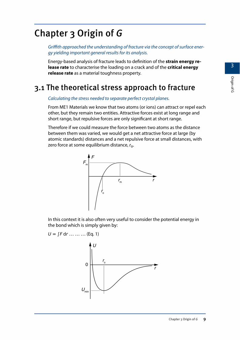
From ME1 Materials we know that two atoms (or ions) can attract or repel eachother, but they remain two entities. Attractive forces exist at long range andshort range, but repulsive forces are only significant at short range.
Therefore if we could measure the force between two atoms as the distancebetween them was varied, we would get a net attractive force at large (byatomic standards) distances and a net repulsive force at small distances, withzero force at some equilibrium distance, ro.
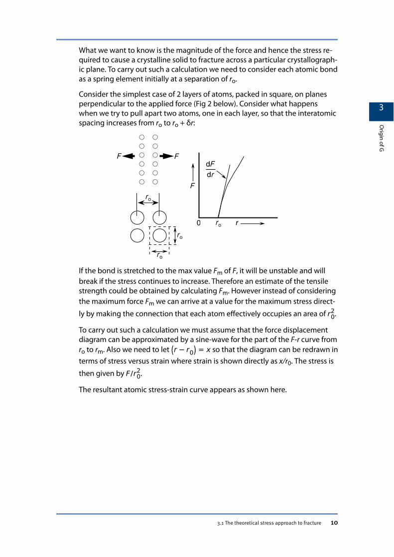
In this context it is also often very useful to consider the potential energy inthe bond which is simply given by:
U = ∫F dr … … … (Eq. 1)
3
Origin of G
Chapter 3 Origin of G 9
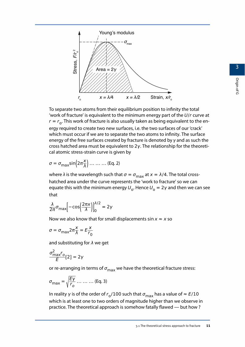
What we want to know is the magnitude of the force and hence the stress re-quired to cause a crystalline solid to fracture across a particular crystallograph-ic plane. To carry out such a calculation we need to consider each atomic bondas a spring element initially at a separation of ro.
Consider the simplest case of 2 layers of atoms, packed in square, on planesperpendicular to the applied force (Fig 2 below). Consider what happenswhen we try to pull apart two atoms, one in each layer, so that the interatomicspacing increases from ro to ro + δr:
r
If the bond is stretched to the max value Fm of F, it will be unstable and willbreak if the stress continues to increase. Therefore an estimate of the tensilestrength could be obtained by calculating Fm. However instead of consideringthe maximum force Fm we can arrive at a value for the maximum stress direct-
ly by making the connection that each atom effectively occupies an area of r02.
To carry out such a calculation we must assume that the force displacementdiagram can be approximated by a sine-wave for the part of the F-r curve fromro to rm. Also we need to let r − r0 = x so that the diagram can be redrawn interms of stress versus strain where strain is shown directly as x/r0. The stress is
then given by F/r02.
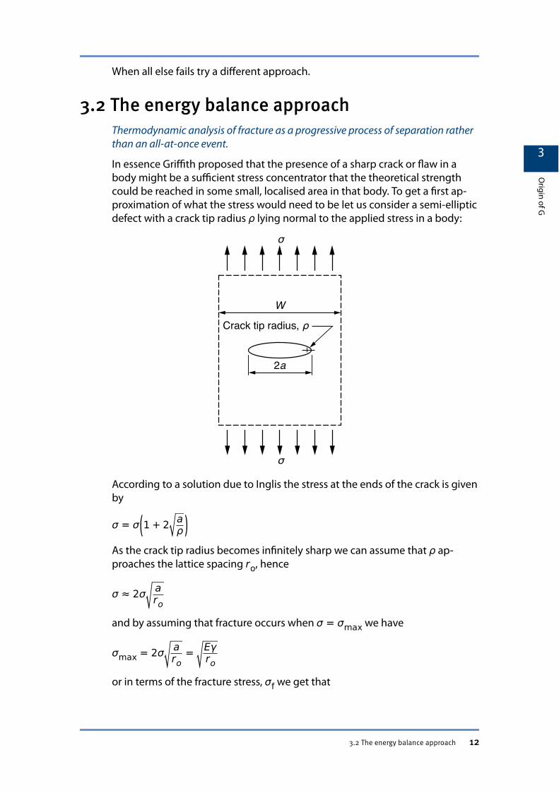
The resultant atomic stress-strain curve appears as shown here.
3
Origin of G
3.1 The theoretical stress approach to fracture 10
To separate two atoms from their equilibrium position to infinity the total‘work of fracture’ is equivalent to the minimum energy part of the U/r curve atr = ro. This work of fracture is also usually taken as being equivalent to the en-ergy required to create two new surfaces, i.e. the two surfaces of our ‘crack’which must occur if we are to separate the two atoms to infinity. The surfaceenergy of the free surfaces created by fracture is denoted by γ and as such thecross hatched area must be equivalent to 2γ. The relationship for the theoreti-cal atomic stress-strain curve is given by
σ = σmaxsin 2πxλ … … … (Eq. 2)
where λ is the wavelength such that σ = σmax at x = λ/4. The total cross-hatched area under the curve represents the ‘work to fracture’ so we canequate this with the minimum energy Uo. Hence Uo = 2γ and then we can seethat
λ2πσmax −cos 2πx
λ 0
λ/2= 2γ
Now we also know that for small displacements sin x ≈ x so
σ = σmax2πxλ = E xr0and substituting for λ we get
σmax2 roE 2 = 2γ
or re-arranging in terms of σmax we have the theoretical fracture stress:
σmax = Eγro
… … … (Eq. 3)
In reality γ is of the order of ro/100 such that σmax has a value of ≈ E/10which is at least one to two orders of magnitude higher than we observe inpractice. The theoretical approach is somehow fatally flawed — but how ?
3
Origin of G
3.1 The theoretical stress approach to fracture 11
When all else fails try a different approach.
3.2 The energy balance approachThermodynamic analysis of fracture as a progressive process of separation ratherthan an all-at-once event.
In essence Griffith proposed that the presence of a sharp crack or flaw in abody might be a sufficient stress concentrator that the theoretical strengthcould be reached in some small, localised area in that body. To get a first ap-proximation of what the stress would need to be let us consider a semi-ellipticdefect with a crack tip radius ρ lying normal to the applied stress in a body:
According to a solution due to Inglis the stress at the ends of the crack is givenby
σ = σ 1 + 2 aρ
As the crack tip radius becomes infinitely sharp we can assume that ρ ap-proaches the lattice spacing ro, hence
σ ≈ 2σ aro
and by assuming that fracture occurs when σ = σmax we have
σmax = 2σ aro
= Eγro
or in terms of the fracture stress, σf we get that
3
Origin of G
3.2 The energy balance approach 12
σf = Eγ4a . … … … (Eq. 4)
If we put a few numerical values in, as before, we can see immediately that adefect length of even a few microns is sufficient to lower the fracture strengthby two orders of magnitude. This approach therefore looks attractive but hasserious limitations in that it assumes too much by taking a totally elastic solu-tion (Inglis) to predict a stress which experience tells us is far from elastic.
Griffith overcame these objections by re-casting this approach in thermody-namic terms in order to get away from having to consider any of the crack tipprocesses.
Consider an infinite plate containing a central, through thickness crack oflength 2a and subjected to a remotely applied uniform tensile stress of σ. Weare in the habit of drawing this configuration as above despite having just sta-ted that the plate is infinite in the x-y plane. What we really mean is that theboundaries of the plate are sufficiently far removed from the ends of the crackthat the fracture process cannot be influenced by the boundaries.
Now consider what happens to the total energy of the system as we extendthe crack by an infinitesimal amount. As the crack extends two new crack sur-faces are created and these surfaces have an associated surface energy of γ/unit area. Thus the energy required to achieve our increment of crack growthis simply 2γ times the area of the new crack surfaces.
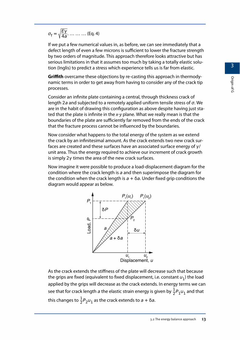
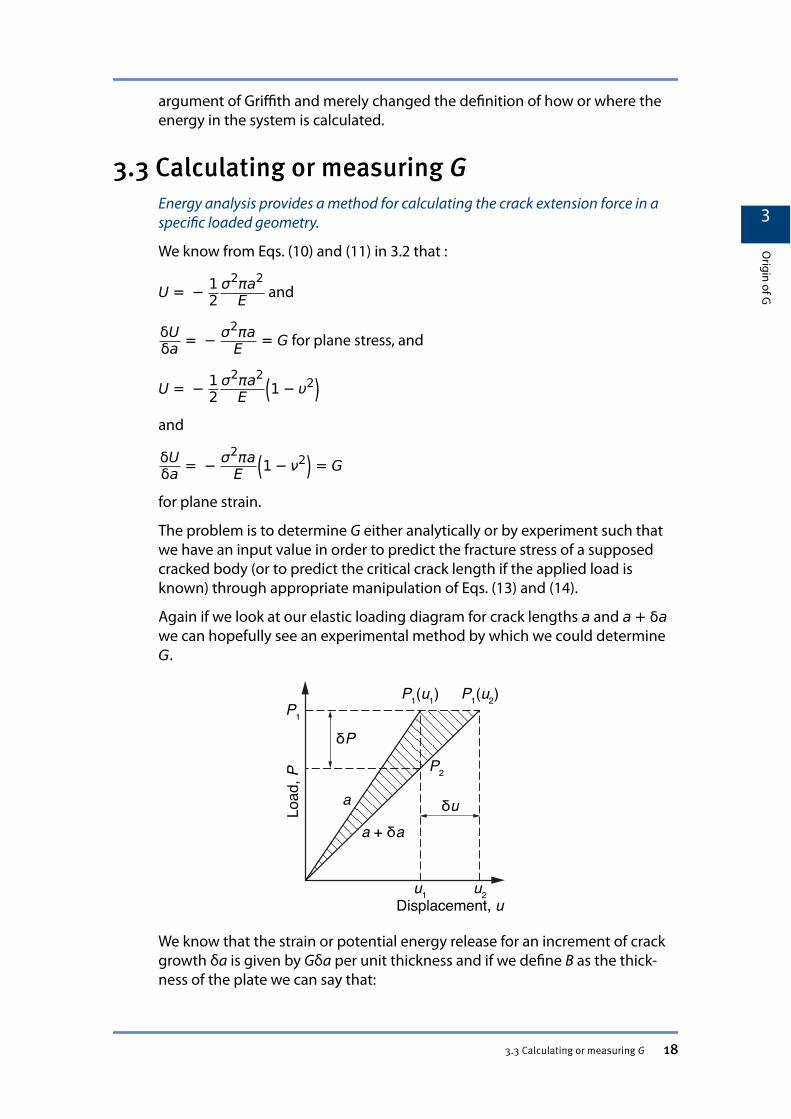
Now imagine it were possible to produce a load-displacement diagram for thecondition where the crack length is a and then superimpose the diagram forthe condition when the crack length is a+ δa. Under fixed grip conditions thediagram would appear as below.
As the crack extends the stiffness of the plate will decrease such that becausethe grips are fixed (equivalent to fixed displacement, i.e. constant u1) the loadapplied by the grips will decrease as the crack extends. In energy terms we cansee that for crack length a the elastic strain energy is given by 12P1u1 and that
this changes to 12P2u1 as the crack extends to a+ δa.
3
Origin of G
3.2 The energy balance approach 13
Hence under fixed grip conditions the extension of the crack from a to a+ δaresults in the release (decrease) of elastic strain energy from the plate equiva-lent to 12 P1− P2 u1.
This release of stored elastic strain energy must go somewhere and intuitivelyit would not seem unreasonable for this energy to be consumed in the work offracture required to create the two new crack surfaces. Before further discus-sing precisely where and how this elastic strain energy is consumed we shouldconsider what happens under fixed loading conditions since this representsthe other end of the spectrum to the assumption of fixed grips or constant dis-placement.
Although a bit more complicated, the same principles apply as for fixed grips.As the crack grows the plate effectively becomes a weaker spring and we needan increase in displacement to keep the load constant. The stored strain ener-gy for the crack of length a+ δa is 12P1u2, which is apparently greater than for
the crack of length a which has an associated elastic strain energy of only12P1u1. However we have to remember that in achieving the increase in crack
length the applied load P has moved through a distance u2− u1 or put anoth-er way we have done work P1 u2− u1 on the system. Thus the overallchange in potential energy of the system is still a decrease expressed as
ΔUE = P1 u2− u1 − 12P1 u2− u1 = 1
2P1 u2− u1 … … … (Eq. 5)
and this quantity of released potential energy is equivalent to the cross hatch-ed area in the load/displacement diagram above.
Now compare the energy released for fixed load with the fixed grip condition.Since we can simplify matters by defining
δu = u2− u1
and
δP = P1− P2
it can be seen that:
strain energy release (fixed grip) = − 12δPu … … … (Eq. 6)
and
potential energy release (constant load) = − 12Pδu … … … (Eq. 7)
Also we need to consider the relationship between load and displacement inthe general case. As for any elastic system the displacement and load are rela-ted through a simple linear equation such that for any given crack length wecan write that
u = CP … … … (Eq. 8)
3
Origin of G
3.2 The energy balance approach 14
where C is a constant referred to as the compliance of the system. (Note that Chas the inverse units to stiffness since compliance is in effect the inverse ofstiffness)
As the increment of crack length δa 0, the value of C will tend to be thesame for a crack of length a and one of length a+ δa. We can therefore re-write Eq. (8) as
δu = CδP … … … (Eq. 9)
and substituting this into Eqs. (6) and (7) we get
− 12δ Pu = − 1
2CP δP
and
− 12Pδu = − 1
2CP δP
In short:
Note
There is no difference in the energy released when an infinitesimally small increment ofcrack growth occurs under conditions of fixed load (potential energy) or conditions of fixedgrips (elastic strain energy).
Griffith made the important connection in recognising that the driving forcefor crack extension is the energy which can be released and that this is usedup as the energy required to create the two new surfaces. This thermodynam-ic description of the fracture process has the huge advantage of removing at-tention from the small area at the crack tip and the precise micromechanismof fracture.
Without going into rigorous detail, Griffith arrived at the following relations forthe change in energy of a body with crack length as follows:
U = − 12σ2πa2E
and
δUδa = − σ
2πaE = G … … … (Eq. 10)
for plane stress and
U = − 12σ2πa2E 1− υ2
and
δUδa = − σ
2πaE 1− υ2 = G … … … (Eq. 11)
for plane strain. The problem is therefore how we get from these equations re-lating energy, applied stress and crack length to some practical relationship
3
Origin of G
3.2 The energy balance approach 15
which predicts the onset of fracture as a function of crack length and appliedstress.
We have seen that δU/δa represents the decrease in potential energy of a sys-tem when a crack extends by a small amount δa under constant load condi-tions.
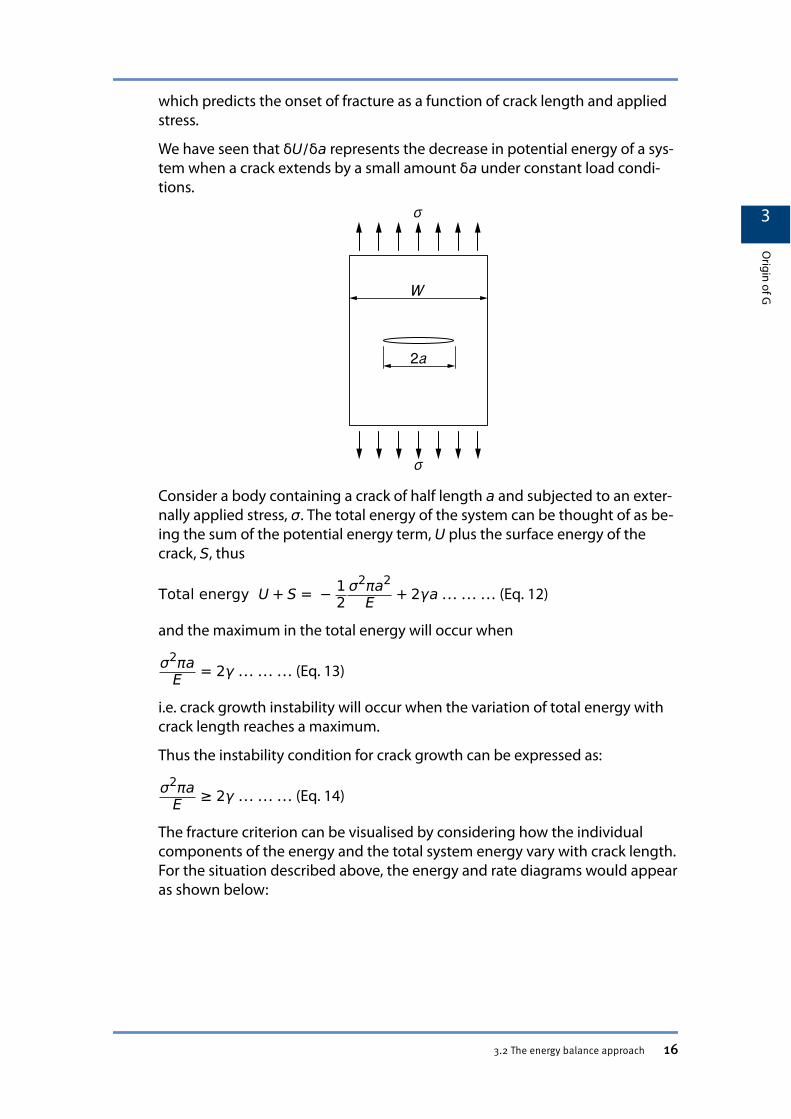
Consider a body containing a crack of half length a and subjected to an exter-nally applied stress, σ. The total energy of the system can be thought of as be-ing the sum of the potential energy term, U plus the surface energy of thecrack, S, thus
Total energy U+ S = − 12σ2πa2E + 2γa … … … (Eq. 12)
and the maximum in the total energy will occur when
σ2πaE = 2γ … … … (Eq. 13)
i.e. crack growth instability will occur when the variation of total energy withcrack length reaches a maximum.
Thus the instability condition for crack growth can be expressed as:
σ2πaE ≥ 2γ … … … (Eq. 14)
The fracture criterion can be visualised by considering how the individualcomponents of the energy and the total system energy vary with crack length.For the situation described above, the energy and rate diagrams would appearas shown below:
3
Origin of G
3.2 The energy balance approach 16
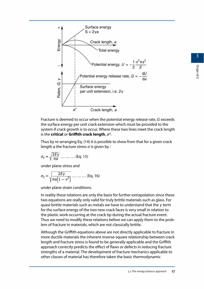
Fracture is deemed to occur when the potential energy release rate, G exceedsthe surface energy per unit crack extension which must be provided to thesystem if crack growth is to occur. Where these two lines meet the crack lengthis the critical or Griffith crack length, a*.
Thus by re-arranging Eq. (14) it is possible to show from that for a given cracklength a the fracture stress σ is given by :
σf = 2Eγπa … … … (Eq. 15)
under plane stress and
σf = 2Eγπa 1− ν2 … … … (Eq. 16)
under plane strain conditions.
In reality these relations are only the basis for further extrapolation since thesetwo equations are really only valid for truly brittle materials such as glass. Forquasi-brittle materials such as metals we have to understand that the γ termfor the surface energy of the two new crack faces is very small in relation tothe plastic work occurring at the crack tip during the actual fracture event.Thus we need to modify these relations before we can apply them to the prob-lem of fracture in materials, which are not classically brittle.
Although the Griffith equations above are not directly applicable to fracture inmore ductile materials the inherent inverse-square relationship between cracklength and fracture stress is found to be generally applicable and the Griffithapproach correctly predicts the effect of flaws or defects in reducing fracturestrengths of a material. The development of fracture mechanics applicable toother classes of material has therefore taken the basic thermodynamic
3
Origin of G
3.2 The energy balance approach 17
argument of Griffith and merely changed the definition of how or where theenergy in the system is calculated.
3.3 Calculating or measuring GEnergy analysis provides a method for calculating the crack extension force in aspecific loaded geometry.
We know from Eqs. (10) and (11) in 3.2 that :
U = − 12σ2πa2E and
δUδa = − σ
2πaE = G for plane stress, and
U = − 12σ2πa2E 1− υ2
and
δUδa = − σ
2πaE 1− ν2 = G
for plane strain.
The problem is to determine G either analytically or by experiment such thatwe have an input value in order to predict the fracture stress of a supposedcracked body (or to predict the critical crack length if the applied load isknown) through appropriate manipulation of Eqs. (13) and (14).
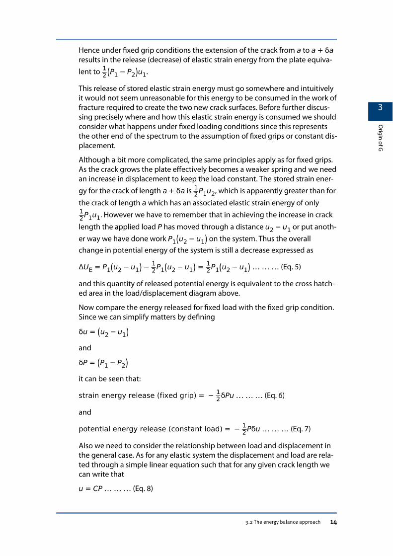
Again if we look at our elastic loading diagram for crack lengths a and a+ δawe can hopefully see an experimental method by which we could determineG.
We know that the strain or potential energy release for an increment of crackgrowth δa is given by Gδa per unit thickness and if we define B as the thick-ness of the plate we can say that:
3
Origin of G
3.3 Calculating or measuring G 18
GδaB = 12Pδu … … … (Eq. 17)
This quantity (the hatched area in the figure) is not easy to measure as δatends to zero, so invoking the compliance relationship in Eq. (6) we can rear-range the relationship as follows:
GBδa = 12P
2δC … … … (Eq. 18)
and as δa tends to zero we have that:
G = P22B∂C∂a … … … (Eq. 19)
and this important relation can be shown to hold for both fixed grip and con-stant load situations.
Hence there are many situations, especially for small test pieces, where G canbe found as a function of crack length by determining the compliance func-tion for the specimen through experiment. A specimen of known dimensionsis initially loaded elastically to measure its compliance at effectively 'zero'crack length. The specimen then has the crack length increased either by ma-chining or through controlled fatigue crack growth and at each increment ofcrack growth the elastic compliance is determined. A graph of compliance as afunction of crack length is then plotted and δC/δa is found for each incrementof crack length either by drawing tangents to the compliance-crack lengthcurve or by numerical techniques.
Compliance,
Load
, P
Displacement, u
Com
plian
ce, C
Crack length, a
at crack lengtha
Caution
Although the tangent method is a tedious procedure, faster numerical methods must berigorously thought through. Most data curve fitting routines use polynomials which cannotbe simply differentiated to give a monotonic function since they are by definition nth orderexpressions which differentiate to n− 1 order expressions.
3
Origin of G
3.3 Calculating or measuring G 19
Norm
alise
d G
func
tion
Normalised crack length, a/W
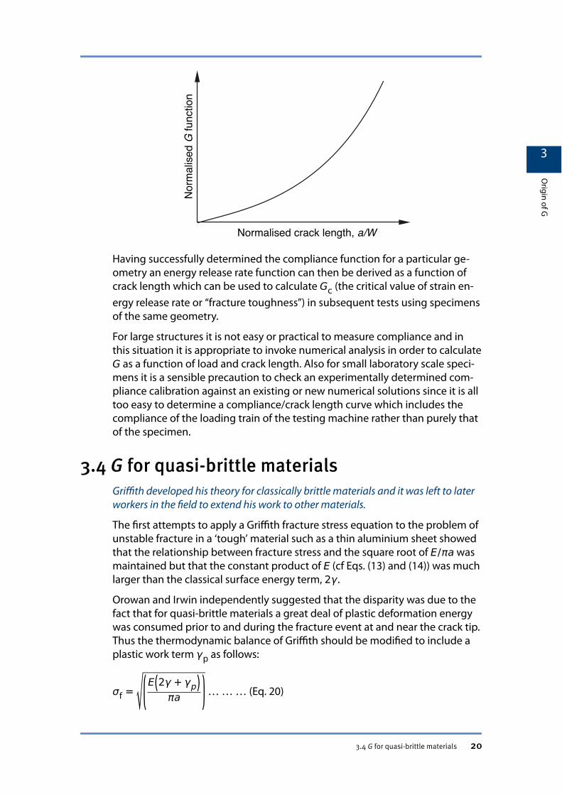
Having successfully determined the compliance function for a particular ge-ometry an energy release rate function can then be derived as a function ofcrack length which can be used to calculate Gc (the critical value of strain en-ergy release rate or “fracture toughness”) in subsequent tests using specimensof the same geometry.
For large structures it is not easy or practical to measure compliance and inthis situation it is appropriate to invoke numerical analysis in order to calculateG as a function of load and crack length. Also for small laboratory scale speci-mens it is a sensible precaution to check an experimentally determined com-pliance calibration against an existing or new numerical solutions since it is alltoo easy to determine a compliance/crack length curve which includes thecompliance of the loading train of the testing machine rather than purely thatof the specimen.
3.4 G for quasi-brittle materialsGriffith developed his theory for classically brittle materials and it was left to laterworkers in the field to extend his work to other materials.
The first attempts to apply a Griffith fracture stress equation to the problem ofunstable fracture in a ‘tough’ material such as a thin aluminium sheet showedthat the relationship between fracture stress and the square root of E/πa wasmaintained but that the constant product of E (cf Eqs. (13) and (14)) was muchlarger than the classical surface energy term, 2γ.
Orowan and Irwin independently suggested that the disparity was due to thefact that for quasi-brittle materials a great deal of plastic deformation energywas consumed prior to and during the fracture event at and near the crack tip.Thus the thermodynamic balance of Griffith should be modified to include aplastic work term γp as follows:
σf =E 2γ + γp
πa … … … (Eq. 20)
3
Origin of G
3.4 G for quasi-brittle materials 20
but since γp ≫ γ the surface energy term can be ignored altogether with nogreat loss of accuracy, hence:
σf =Eγpπa … … … (Eq. 21)
This simplification has attractions since, by carrying out a few simple tests withcracks of differing lengths, a value for γp can be found directly and used as ameans of predicting the onset of brittle fracture under other conditions of ap-plied load and crack length. In practice this type of procedure is rarely carriedout since the conditions under which reproduceable fracture toughness re-sults can be measured are better understood and implemented for the stressintensity factor approach to fracture.
As will be demonstrated later it can be shown that the strain energy releaserate approach to prediction of crack instability through Gc and the comple-mentary idea of the critical value of stress intensity factor are simply relatedand are thus to a large extent interchangeable. If anything, the concept of acritical value of strain (or potential) energy release rate is a more rigorous ap-proach which gives a better model of the fracture process but is rather lesseasy to manipulate than the equivalent idea of a critical value of stress intensi-ty at fracture.
3
Origin of G
3.4 G for quasi-brittle materials 21
Chapter 4 Origin of KThe analysis of fracture can also be approached via elastic stress analysis of theregion around a sharp-tipped crack.
4.1 Brittle fractureThe characteristics of brittle fracture and examples of materials which demon-strate it.
Materials which can exhibit Brittle Fracture
• Mild steel at low temperature
• High strength Fe, Al and Ti alloys
• Glass
• Perspex
• Ceramics
• Concrete
• Fresh Carrots
Characteristic features of a Brittle Fracture
1. Very little general plasticity — broken pieces can be fitted together withno obvious deformation.
2. Rapid crack propagation (Vs/3), eg ‚ ~1000 m/s for steel
3. Low failure load relative to general yield load.
4. Low energy absorption.
5. Usually fractures are flat and perpendicular to maximum principal stress.
6. Fracture always initiates at a flaw or a site of stress concentration.
4.2 Stress concentration at notchesThe dependence of stress concentration factor on notch length and tip radius.
Low stress brittle fractures occur in components which are loaded elasticallybut contain flaws from fabrication or service (eg porosity, fatigue, corrosion,etc). The fracture instability must therefore be associated in some way withthe concentration of stress in the vicinity of the flaw.
The maximum elastic stress at the tip of an elliptical notch of depth a and rootradius ρ is given by the Inglis solution which we have already seen:
σmax = σnom 1 + 2 aρ ≅ 2σnom
aρ … … … (Eq. 1)
4
Origin of K
Chapter 4 Origin of K 22
In traditional engineering design such stress concentrations are denoted bythe stress concentration factor kt:
kt =σmaxσnom
… … … (Eq. 2)
Caution
Do not confuse the stress concentration factor kt with the stress intensity factor K or KIc.Typical situations where stress concentrations arise are changes of section or point loads.For such situations the use of appropriate kt values in design is essential, particularly in fati-gue design. (kt values for all commonly occurring notch geometries are available in Peters-en, Stress concentration factors).
4.3 Stress concentration at cracksFor an infinitely sharp crack the SCF is infinite, and must be redefined.
For a sharp crack the radius of the tip is extremely small (typically 10–3 to 10–5
mm). Equation (1) predicts that σmax ∞ as ρ 0. This suggests that for asharp crack, any applied stress will cause infinitely high stresses at the tip. Alsofor very sharp cracks, this approach cannot distinguish between long andshort cracks whereas experience tells us that failure stress depends on cracklength.
Conclusion: the concept of stress concentration factor breaks down as cracktip radius tends to zero.
Consider instead the product of σmax at the crack tip and the crack tip radius,ρ:
σmax2 πρ … … … (Eq. 3)
(Numerical factors 2 and π are introduced for later convenience). If we substi-tute for σmax from Eq. (1) and allow ρ 0, Eq. (3) reduces to:
σnom πa … … … (Eq. 4)
This remains finite and is formed from the physical quantities σmax and awhich define the problem. This is a definition of the stress intensity factor K.
4.4 Stress-strain fields ahead of a crackShort description.
The preceding loose definition of K results from considering the stress con-centration effect of a crack in somewhat general terms. A more rigorous analy-sis for the stress analysis of a crack is included here for completeness.
The solutions that follow were compiled in 1948 and became known as theWestergaard solutions. The expressions for the stresses are obtained
4
Origin of K
4.3 Stress concentration at cracks 23
neglecting plasticity in the first instance, i.e. a material is assumed which hasno elastic limit.
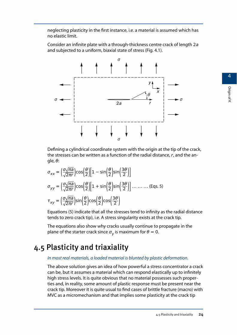
Consider an infinite plate with a through-thickness centre crack of length 2aand subjected to a uniform, biaxial state of stress (Fig. 4.1).
Defining a cylindrical coordinate system with the origin at the tip of the crack,the stresses can be written as a function of the radial distance, r, and the an-gle, θ:
σxx = σ πa2πr cos θ2 1− sin θ
2 sin 3θ2
σyy = σ πa2πr cos θ2 1 + sin θ
2 sin 3θ2
τxy = σ πa2πr sin θ
2 cos θ2 cos 3θ2
… … … (Eqs. 5)
Equations (5) indicate that all the stresses tend to infinity as the radial distancetends to zero crack tip), i.e. A stress singularity exists at the crack tip.
The equations also show why cracks usually continue to propagate in theplane of the starter crack since σy is maximum for θ = 0.
4.5 Plasticity and triaxialityIn most real materials, a loaded material is blunted by plastic deformation.
The above solution gives an idea of how powerful a stress concentrator a crackcan be, but it assumes a material which can respond elastically up to infinitelyhigh stress levels. It is quite obvious that no material possesses such proper-ties and, in reality, some amount of plastic response must be present near thecrack tip. Moreover it is quite usual to find cases of brittle fracture (macro) withMVC as a micromechanism and that implies some plasticity at the crack tip
4
Origin of K
4.5 Plasticity and triaxiality 24
(the very essence of MVC). However, this plasticity also must be somewhatlimited, since cracking occurs before general yield.
The next step is try to describe the extent and geometry of a plastic zonewhich could exist in a stress field described by the Westergaard solutions.
As usual in plasticity analyses, description of the field in terms of principalstresses facilitates visualisation. The principal stresses for the same Wester-gaard field are:
σ1 = σ πa2πr cos θ2 1 + sin θ2
σ2 = σ πa2πr cos θ2 1− sin θ2
… … … (Eq. 6)
Tresca or Von Mises may be used as yield criteria for metals and they are bothindicative of the presence of shear (shear strain energy in the case of Misesand maximum shear stress in Tresca’s case), therefore some assumption mustbe made as to the value of the third principal stress component, σ3. Two possi-bilities are of interest:
1. Plane stress: σ3 = 0;
2. Plane strain: ϵ3 = 0 hence σ3 = ν σ1 + σ2 .
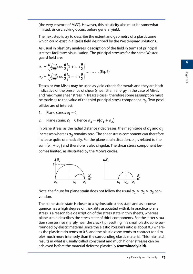
In plane stress, as the radial distance r decreases, the magnitude of σ1 and σ2increases whereas σ3 remains zero. The shear stress component can thereforeincrease quite dramatically. For the plane strain situation, σ3 is related to thesum σ1 + σ1 and therefore is also singular. The shear stress component be-comes limited, as illustrated by the Mohr’s circles.
Note: the figure for plane strain does not follow the usual σ1 > σ2 > σ3 con-vention.
The plane strain state is closer to a hydrostatic stress state and as a conse-quence has a high degree of triaxiality associated with it. In practice, planestress is a reasonable description of the stress state in thin sheets, whereasplane strain describes the stress state of thick components. For the latter situa-tion stresses rise sharply near the crack tip resulting in a small plastic zone sur-rounded by elastic material, since the elastic Poisson’s ratio is about 0.3 where-as the plastic ratio tends to 0.5, and the plastic zone tends to contract (or dim-ple) much more intensely than the surrounding elastic material. This mismatchresults in what is usually called constraint and much higher stresses can beachieved before the material deforms plastically (contained yield).
4
Origin of K
4.5 Plasticity and triaxiality 25
Thick sections are then usually associated with the terms plane strain, highconstraint, high triaxiality, contained yield and higher severity.
Important
The stress analysis of a crack explains how brittle fracture (macro) can occur (regardless ofmicromechanism) when plasticity is contained by an increased level of triaxiality. LARGETHICKNESS implies PLANE STRAIN TRIAXIALITY implies LESS PLASTICITY implies BRITTLEFRACTURE.
4.6 The stress intensity factor and the shapefactor
The definition of a single scaling factor to represent the loading geometry andconfiguration.
Inspection of the equations which describe the stress field ahead of the cracktip indicates that all of the expressions are of the form
12πr(a)
× f θ(b)
× σ πa(c)
• Term (a) represents the singularity since this term ∞ as the radial dis-tance, r 0.
• Term (b) describes the variation with respect to the angle θ and is limited(consider the trigonometric functions).
• Term (c) is a simple function of remote stress σ and crack length a. Thissimple function dictates the intensity or the magnitude of the stress fieldand is called the stress intensity factor, K.
Important
The stress intensity factor, K, is a single parameter which completely specifies the ampli-tude of the stress field in the vicinity of the crack tip.
For the initial case of the infinite plate subjected to uniform stresses, the stressintensity factor is written
K = σ πa … … … (Eq. 9)
which is justifiable since, for an infinite plate, the only known dimension is thecrack length.
In general, the stress intensity factor depends on the geometry of the crackedbody (including the crack length) and it is usual to express it as
K = Yσ a … … … (Eq. 10)
where Y is called the shape factor and is a function of body geometry andcrack length.
4
Origin of K
4.6 The stress intensity factor and the shape factor 26
Caution
The π term is included in the Y factor, but some authorities and textbooks refer to theinfinite plate case (Eq 9) and leave the fundamental σ πa term outside the Y. You will seeboth definitions!
4.7 Modifications for real geometriesShort description.
The above expression for K is applicable to an ideal situation of an infiniteplate containing a centre crack of length 2a. In practice the presence of finiteboundaries and the way in which the crack is loaded affects the value of thestress intensity factor.
● Loading geometry
A crack can be loaded in three ways.
Mode I
has the crack opening under the influence of a stress at right angles tothe crack plane;
Mode II
involves in-plane sliding normal to the crack front under the influence ofa shear stress parallel to the crack plane;
Mode III
involves in-plane sliding parallel to the crack front under the influence ofa shear stress parallel to the crack plane.
Stress intensities can be defined for each type of displacement and are desig-nated KI, KII and KIII. However, the great majority of failures occur under modeI loading and hence most fracture toughness data relate to this mode of load-ing. For mode I loading, the critical stress intensity factor is designated KIc.
● Component geometry
The geometry of the cracked body imposes an effect on the near crack tipstress field and hence modifies the value of the stress intensity factor. For realgeometries K is defined above as:
K = Yσ a
Y is the geometrical factor which is dependent on crack length and specimendimensions.
4
Origin of K
4.7 Modifications for real geometries 27
A commonly encountered Y factor is for a straight-fronted edge crack. If thecrack length a is small in proportion to the component depth, then Y = 1.99,i.e. the open edge allows K to increase by 12%.
1. For a centre cracked plate of finite width:
KI = Yσ a
Y = sec πaW1/2
.
So… given the width W, the applied stress σ and the crack length a, theapplied stress intensity factor KI can be calculated.
2. For an edge notch in tension:
KIc = Yσ a
Y = 1.99 for small cracks, otherwise:
Y = 1.99− 0.41 aW + 18.7 a
W2− 38.48 a
W3 + 53.85 a
W4
.
Y factors for most other crack geometries are available.
4.8 Critical stress intensity factor KIc: a fracturecriterion
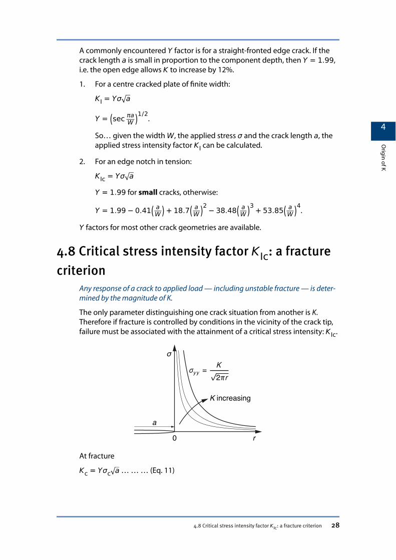
Any response of a crack to applied load — including unstable fracture — is deter-mined by the magnitude of K.
The only parameter distinguishing one crack situation from another is K.Therefore if fracture is controlled by conditions in the vicinity of the crack tip,failure must be associated with the attainment of a critical stress intensity: KIc.
At fracture
Kc = Yσc a … … … (Eq. 11)
4
Origin of K
4.8 Critical stress intensity factor KIc: a fracture criterion 28
In practice we may attain KIc by increasing either σ or a. For a defect of fixedlength a, σf is the critical value of the applied stress for fracture. Alternatively,for a constant applied stress σ, ac is the critical defect size for fracture.
KIc is a macroscopic criterion for failure. It makes no assumptions about theprecise mechanism of fracture.
Note
K is a stress field parameter independent of the material, whereas KIc is a material property,the fracture toughness. (Compare stress σ which can have any value, and σy which is aspecific material property).
The units of K are (stress)√(distance). This may be written most clearly asMPa√m but usually appears as MN m–3/2 or occasionally as N mm–3/2.
Important
The stress used in evaluating the K parameter, and in all fracture mechanics calculations, isthe nominal stress acting on the body in the vicinity of the defect; it must not take into con-sideration any loss of section caused by the presence of the defect.
4.9 Component thicknessDue to crack-tip plasticity, the value of Kc is influenced by component thickness.
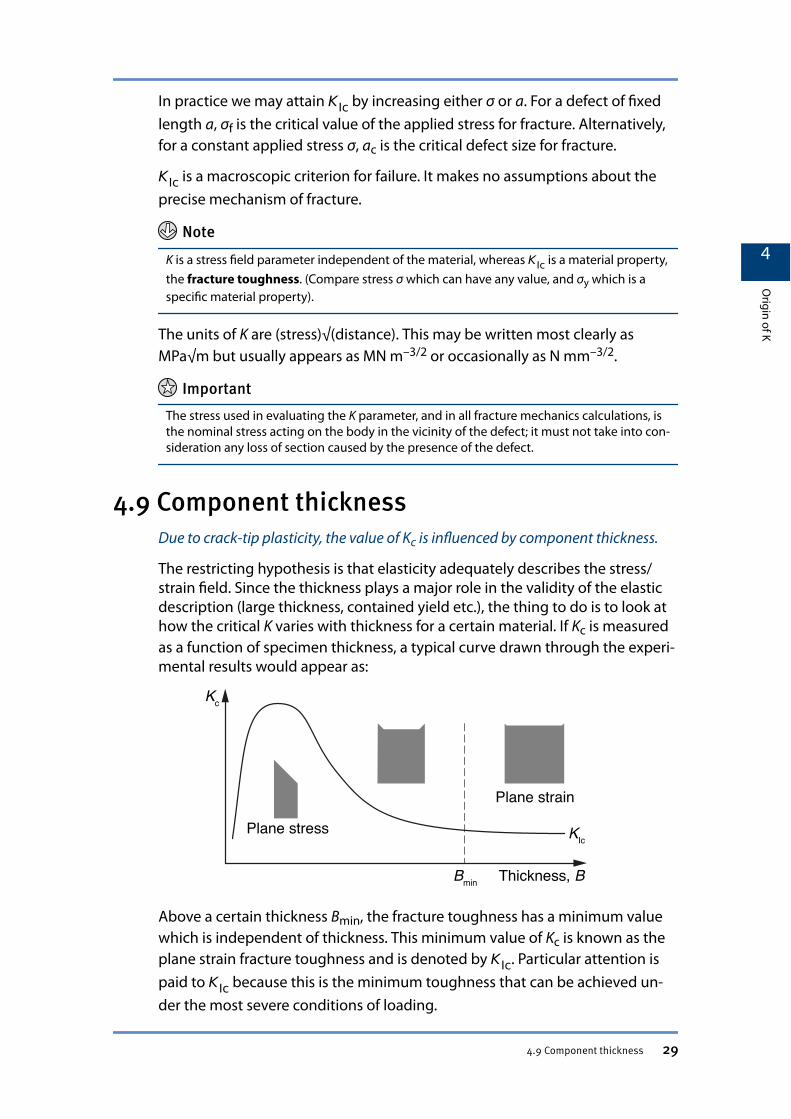
The restricting hypothesis is that elasticity adequately describes the stress/strain field. Since the thickness plays a major role in the validity of the elasticdescription (large thickness, contained yield etc.), the thing to do is to look athow the critical K varies with thickness for a certain material. If Kc is measuredas a function of specimen thickness, a typical curve drawn through the experi-mental results would appear as:
Above a certain thickness Bmin, the fracture toughness has a minimum valuewhich is independent of thickness. This minimum value of Kc is known as theplane strain fracture toughness and is denoted by KIc. Particular attention ispaid to KIc because this is the minimum toughness that can be achieved un-der the most severe conditions of loading.
4
Origin of K
4.9 Component thickness 29
The minimum specimen thickness required to ensure the plane strain condi-tions necessary for KIc is given by:
Bmin = 2.5KIcσy
2 … … … (Eq. 12)
As the specimen thickness decreases from Bmin, the fracture toughness KIc in-creases until a maximum value is attained. This maximum reflects the attain-ment of fully plane stress conditions. Thereafter the toughness again decrea-ses for very small thicknesses.
The changes in KIc with thickness are accompanied by corresponding changesin fracture geometry. In the plane strain regime the fracture surface is orientedat 90° to the direction of loading (ie “square” fracture). As the thickness decrea-ses, 45° “shear lips” appear on either side of a flat central regime. At and belowthe thickness corresponding to the maximum KIc position, the shear lips occu-py the full thickness and one has a 45° “shear” or plane stress fracture.
Note
For any thickness of material, the fracture may be completely brittle in the engineeringsense, irrespective of the fracture surface geometry or whether plane stress or plane strainloading conditions prevail.
4.10 Inter-relationship of Kc and GcShort description.
The strain energy approach to brittle fracture gives:
σf = E2γπa =
EGCπa
for plane stress conditions and
σf = 2Eγπa 1− ν2 =
EG1Cπa 1− ν2
(GIc = plane strain critical strain energy release rate) for plane strain conditions.Substituting for K from Eq. (9) gives the relationship at brittle fracture:
Kc2 = EGc under plane stress loading conditions … … … (Eq. 13)
(or in the general case K2 = EG for plane stress loading) and
K1c2 = EG1C under plane strain loading conditions … … … (Eq. 14)
where
G = πσ2aE
4
Origin of K
4.10 Inter-relationship of Kc and Gc 30
is the elastic energy release rate and is named after Griffith. G has dimensionsof energy per unit area (cracked area).
It follows that a measured value of K1c can be converted to a value of GIc andvice-versa, the main underlying assumption being that linear elasticity de-scribes the stress/strain field adequately. Both GIc and KIc are called the frac-ture toughness of a material.
4.11 Stress ahead of the crack tipThe component of local stress acting across the crack line is singular, but the othercomponents show different forms.
So far we have considered the elastic stress normal to the crack plane, i.e.σyy = K
2πr . Note σyy is in the same direction as σnom and arises from the stress
concentrating effect of the crack.
What about stresses in x and z directions?
● The x-direction
The region of stress intensification is confined to a small region (≈a/10) aheadof crack tip. Outside this region, the material experiences the nominal elasticstress, σnom.
Consider an element of material located within the highly stressed regionwhich is exposed to σyy = K
2πr .
If treated as an isolated, uniaxial tensile specimen, it would extend elastically
to give a strain commensurate with the local stress, ie ϵyy =σyyE and contract
laterally by -υε, the Poisson contraction.
But because the surrounding material in the x direction stops the contraction,ie a σx stress develops due to constraint.
At a blunted crack tip we have a small area of free surface normal to the x di-rection, hence at this position σxx = 0. However, as we enter the crack tipzone σxx tends to σyy.
Ahead of the crack tip‚
σxx = σyy = K2πr
● The z-direction
For thin sheet there is zero stress in the thickness direction, i.e. σzz = 0 butthere will be a thickness strain which manifests itself as a local sucking in or‘notch root contraction’. This condition is known as plane stress.
4
Origin of K
4.11 Stress ahead of the crack tip 31
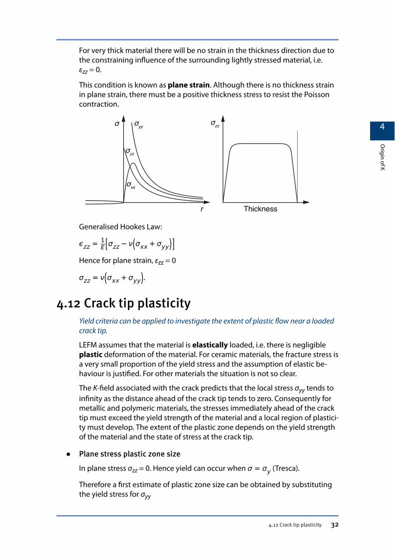
For very thick material there will be no strain in the thickness direction due tothe constraining influence of the surrounding lightly stressed material, i.e.εzz = 0.
This condition is known as plane strain. Although there is no thickness strainin plane strain, there must be a positive thickness stress to resist the Poissoncontraction.
Generalised Hookes Law:
ϵzz = 1E σzz− ν σxx+ σyy
Hence for plane strain‚ εzz = 0
σzz = ν σxx+ σyy .
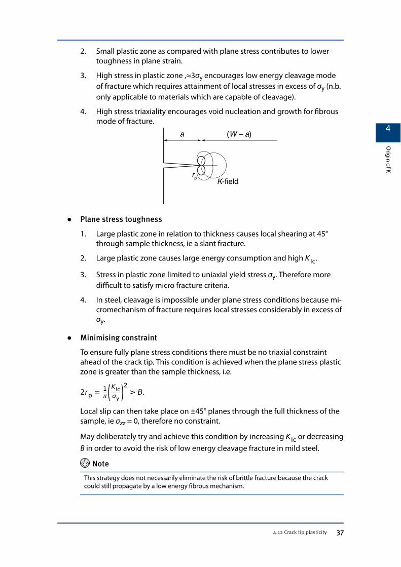
4.12 Crack tip plasticityYield criteria can be applied to investigate the extent of plastic flow near a loadedcrack tip.
LEFM assumes that the material is elastically loaded, i.e. there is negligibleplastic deformation of the material. For ceramic materials, the fracture stress isa very small proportion of the yield stress and the assumption of elastic be-haviour is justified. For other materials the situation is not so clear.
The K-field associated with the crack predicts that the local stress σyy tends toinfinity as the distance ahead of the crack tip tends to zero. Consequently formetallic and polymeric materials, the stresses immediately ahead of the cracktip must exceed the yield strength of the material and a local region of plastici-ty must develop. The extent of the plastic zone depends on the yield strengthof the material and the state of stress at the crack tip.
● Plane stress plastic zone size
In plane stress σzz = 0. Hence yield can occur when σ = σy (Tresca).
Therefore a first estimate of plastic zone size can be obtained by substitutingthe yield stress for σyy
4
Origin of K
4.12 Crack tip plasticity 32
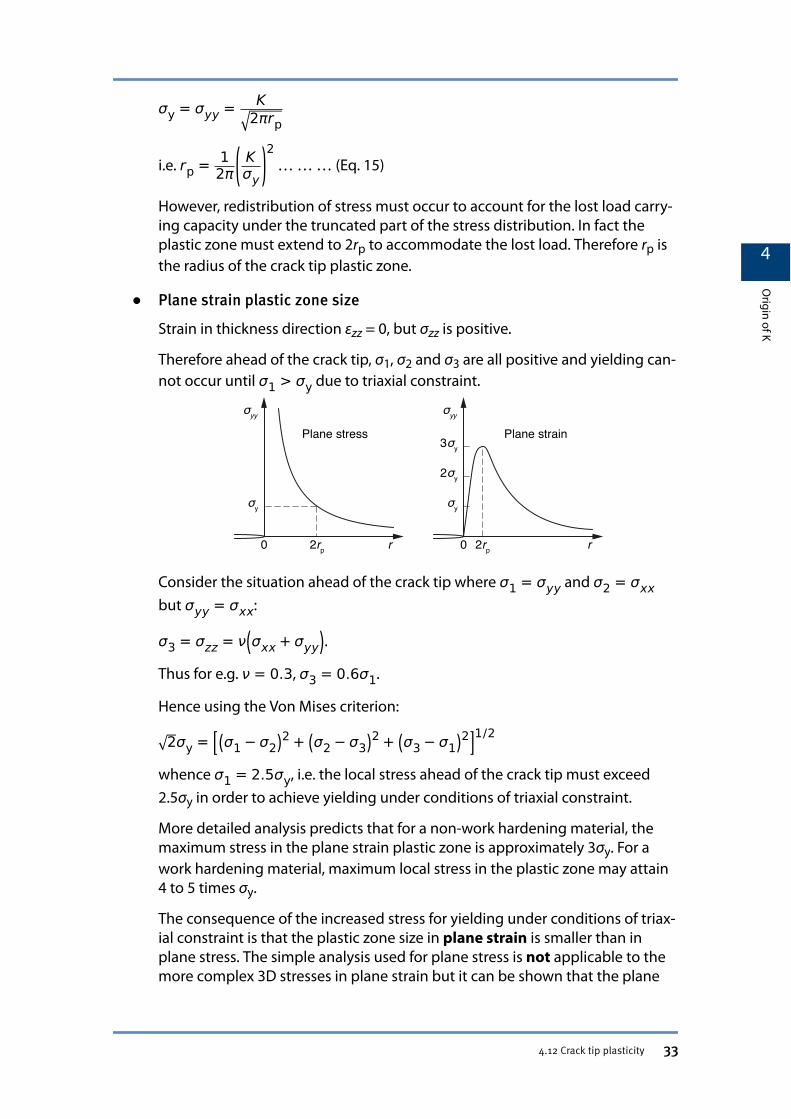
σy = σyy = K2πrp
i.e. rp = 12π
Kσy
2 … … … (Eq. 15)
However, redistribution of stress must occur to account for the lost load carry-ing capacity under the truncated part of the stress distribution. In fact theplastic zone must extend to 2rp to accommodate the lost load. Therefore rp isthe radius of the crack tip plastic zone.
● Plane strain plastic zone size
Strain in thickness direction εzz = 0, but σzz is positive.
Therefore ahead of the crack tip, σ1, σ2 and σ3 are all positive and yielding can-not occur until σ1 > σy due to triaxial constraint.
Consider the situation ahead of the crack tip where σ1 = σyy and σ2 = σxxbut σyy = σxx:
σ3 = σzz = ν σxx+ σyy .
Thus for e.g. ν = 0.3, σ3 = 0.6σ1.
Hence using the Von Mises criterion:
2σy = σ1− σ22 + σ2− σ3
2 + σ3− σ12 1/2
whence σ1 = 2.5σy, i.e. the local stress ahead of the crack tip must exceed2.5σy in order to achieve yielding under conditions of triaxial constraint.
More detailed analysis predicts that for a non-work hardening material, themaximum stress in the plane strain plastic zone is approximately 3σy. For awork hardening material, maximum local stress in the plastic zone may attain4 to 5 times σy.
The consequence of the increased stress for yielding under conditions of triax-ial constraint is that the plastic zone size in plane strain is smaller than inplane stress. The simple analysis used for plane stress is not applicable to themore complex 3D stresses in plane strain but it can be shown that the plane
4
Origin of K
4.12 Crack tip plasticity 33
strain plastic zone size is approximately 1/3 of that in plane stress and is givenby:
rp = 16π
KIσy
2 … … … (Eq. 16)
Note
The above expressions for rp have used K and KI rather than Kc and KIc. This is because therewill be a plastic zone associated with the crack for any applied stress intensity K. When the Kvalue reaches the critical value, Kc, the plastic zone will have achieved its maximum size.Thus for plane strain,
rp = 16π
KIcσy
2 … … … (Eq. 17)
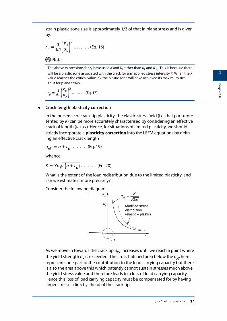
● Crack length plasticity correction
In the presence of crack tip plasticity, the elastic stress field (i.e. that part repre-sented by K) can be more accurately characterised by considering an effectivecrack of length (a + rp). Hence, for situations of limited plasticity, we shouldstrictly incorporate a plasticity correction into the LEFM equations by defin-ing an effective crack length
aeff = a+ rp … … … (Eq. 19)
whence
K = Yσ π a+ rp … … … (Eq. 20)
What is the extent of the load redistribution due to the limited plasticity, andcan we estimate it more precisely?
Consider the following diagram.
As we move in towards the crack tip σyy increases until we reach a point wherethe yield strength σy is exceeded. The cross hatched area below the σyy hererepresents one part of the contribution to the load carrying capacity but thereis also the area above this which patently cannot sustain stresses much abovethe yield stress value and therefore leads to a loss of load carrying capacity.Hence this loss of load carrying capacity must be compensated for by havinglarger stresses directly ahead of the crack tip.
4
Origin of K
4.12 Crack tip plasticity 34
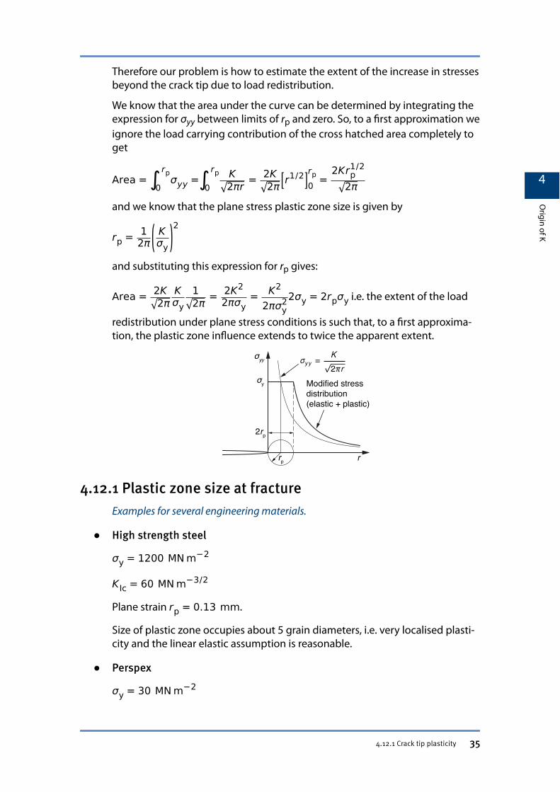
Therefore our problem is how to estimate the extent of the increase in stressesbeyond the crack tip due to load redistribution.
We know that the area under the curve can be determined by integrating theexpression for σyy between limits of rp and zero. So, to a first approximation weignore the load carrying contribution of the cross hatched area completely toget
Area =∫0rpσyy =∫0
rp K2πr = 2K
2π r1/2
0rp =
2Krp1/2
2πand we know that the plane stress plastic zone size is given by
rp = 12π
Kσy
2
and substituting this expression for rp gives:
Area = 2K2π
Kσy
12π = 2K2
2πσy= K2
2πσy22σy = 2rpσy i.e. the extent of the load
redistribution under plane stress conditions is such that, to a first approxima-tion, the plastic zone influence extends to twice the apparent extent.
4.12.1 Plastic zone size at fractureExamples for several engineering materials.
● High strength steel
σy = 1200 MN m−2
KIc = 60 MN m−3/2
Plane strain rp = 0.13 mm.
Size of plastic zone occupies about 5 grain diameters, i.e. very localised plasti-city and the linear elastic assumption is reasonable.
● Perspex
σy = 30 MN m−2
4
Origin of K
4.12.1 Crack tip plasticity 35
KIc = 1 MN m−3/2
Plane strain rp = 60 μm.
Still a very small value in comparison with dimensions of sheet etc. ThereforeLEFM reasonable.
● Alumina
σy = 5000 MN m−2
KIc = 1 MN m−3/2
Plane strain rp = 2 nm.Extent of any plasticity would be comparable with interatomic dimensions, i.e.effectively non-existent.
● Structural steel
σy = 400 MN m−2
Plane strain KIc = 150 MN m−3/2
For thick sections rp = 7.5 mm.
Plane stress Kc = 250 MN m−3/2
For thin sections rp = 60 mm
(Must question whether LEFM assumptions are valid for large plastic zones inlower strength metallic materials).
4.12.2 Consequences of crack tip plasticity on toughnessBecause toughness is related to plastic surface work, its value is partly determinedby yield stress/strain properties.
The development of a plastic zone is by far the major source of energy con-sumption in a fracture process, i.e. crack tip plasticity is the source of tough-ness. This is why ceramics and high strength metals have poor toughness.
Remember that:
• KIc2 = EGIc and GIc = 2γs;
• The true surface energy γs = 2 J m−2; and
• For metallic materials GIc = 2 γs + γp ≈ 104 J m−2.
● Plane strain toughness
1. Small plastic zone in relation to sample thickness causes fracture surfaceto be oriented at right angles to applied stress, i.e. a square fracture.
4
Origin of K
4.12.2 Crack tip plasticity 36
2. Small plastic zone as compared with plane stress contributes to lowertoughness in plane strain.
3. High stress in plastic zone ‚≈3σy encourages low energy cleavage modeof fracture which requires attainment of local stresses in excess of σy (n.b.only applicable to materials which are capable of cleavage).
4. High stress triaxiality encourages void nucleation and growth for fibrousmode of fracture.
● Plane stress toughness
1. Large plastic zone in relation to thickness causes local shearing at 45°through sample thickness, ie a slant fracture.
2. Large plastic zone causes large energy consumption and high KIc.
3. Stress in plastic zone limited to uniaxial yield stress σy. Therefore moredifficult to satisfy micro fracture criteria.
4. In steel, cleavage is impossible under plane stress conditions because mi-cromechanism of fracture requires local stresses considerably in excess ofσy.
● Minimising constraint
To ensure fully plane stress conditions there must be no triaxial constraintahead of the crack tip. This condition is achieved when the plane stress plasticzone is greater than the sample thickness, i.e.
2rp = 1πKIcσy
2> B.
Local slip can then take place on ±45° planes through the full thickness of thesample, ie σzz = 0, therefore no constraint.
May deliberately try and achieve this condition by increasing KIc or decreasingB in order to avoid the risk of low energy cleavage fracture in mild steel.
Note
This strategy does not necessarily eliminate the risk of brittle fracture because the crackcould still propagate by a low energy fibrous mechanism.
4
Origin of K
4.12 Crack tip plasticity 37
4.12.3 Constraints on LEFM validityA summary of the limits within which LEFM assumptions are justifiable.
1. Characterisation of elastic crack tip stresses by K is valid only for the re-gion immediately ahead of the crack tip, i.e. for a/10 ahead of tip.
2. Embedded within the elastic field is the plastic zone:
rp = 12π
Kcσy
2 for plane stress.
3. For events in the plastic zone to be controlled by the surrounding K field,i.e. for crack tip processes to be controlled by K, the plastic zone size mustby less than 20% of the K field, ie . rp < a/50.
4. Similar contraints apply to the next section below the crack (W – a) ierp < W − a /50.
5. Conclude that for LEFM (plane stress and plane strain):
a, (W - a) > 50rp.
6. For plane strain there is an additional requirement that the size of theplastic zone must be less than 1/50 of the thickness B, ie B > 50rp.
rp = 16π
KIcσy
2 for plane strain so that:
a, (W - a), B > 2.5KIcσy
2.
4.12.4 Practical implications of crack tip plasticityThe applicability of LEFM to some specific structural materials.
● High strength and/or brittle materials
For high strength and brittle materials the plastic zone size is small, and themacroscopic fracture behaviour is dominated by the elastic stresses in the ma-terial.
1. High strength aluminium alloyKIc = 25 MN m−3/2
σy = 500 MN m−2
Plane strain rp = 0.13 mm
For LEFM plane strain Bmin = 6 mm.
2. High strength steel
KIc = 60 MN m−3/2
4
Origin of K
4.12.3 Crack tip plasticity 38
σy = 1500 MN m−2
rp = 0.10 mm
For LEFM plane strain Bmin = 5 mm.
3. PMMA (Perspex)
KIc = 1.5 MN m−3/2
σy = 50 MN m−2
rp = 0.05 mm
For LEFM plane strain Bmin = 2.5 mm.Conclusion: for these materials LEFM fracture mechanics works OK.
● Medium strength structural steel
σy = 450 MN m−2
KIc = 80 MN m−3/2
Plane strain rp = 1.7 mm
For LEFM plane strain Bmin = 85 mm.In the light of the large Bmin value necessary for LEFM plane strain validity it isnecessary to consider two different service situations:
● Applications requiring thick sections
Example: Nuclear pressure vessel where the wall thickness may be 200 mm.
LEFM is then appropriate to the service situation and KIc values should beused for the prediction of critical defect sizes and specification of acceptabledefects.
The problem then is how to measure KIc to characterise the fracture tough-ness of the steel used. For the laboratory test we still need to satisfy the condi-tions for LEFM plane strain validity: a, (W – a) and B > 85 mm.
This may be possible but would be highly impracticable and very costly. If weuse a small specimen, we no longer have plane strain conditions, have exten-sive plasticity and the toughness measurement in terms of KIc is no longermeaningful.Conclusion: We need an alternative method of measuring toughness.
● Applications requiring thin sections
Application is such that material is used in sections much thinner than Bmin,e.g. ship’s deck or pipeline where the plate thickness may be say 15 mm. For
4
Origin of K
4.12 Crack tip plasticity 39
this situation the use of KIc to predict failure would be excessively conserva-
tive. For example, whilst the KIc value might be 80 MN m–3/2, the KIc value
appropriate to a plate thickness of 15 mm might be 240 MN m–3/2. This equa-tes to an almost 10-fold increase in critical defect size.
In principle we could determine the KIc value appropriate to the thickness ofthe plate. However, during such laboratory testing we would still have to satis-fy the conditions for LEFM plane stress validity namely:
a, (W–a) > 50rp.
For KIc = 240 MN m–3/2, rp = 45 mm, i.e. we would need a test panel at least2.25 m wide. Again testing is impracticable and we need an alternative meth-od of assessing toughness.
4.12.5 Material fracture toughness dataData from Ashby and Jones, Engineering Materials 1.
All values are at room temperature except *.
Material Gc (kJ m–2) KIc (MN m–3/2)
Pure ductile metals e.g. Cu, Al, Ni, Ag 100–1000 100–350
Rotor Steels 220–240 204–214
Pressure Vessel Steels e.g. HY 130 150 170
High Strength Steels 15–118 50–154
Mild Steel 100 140
Ti Alloys (Ti 6Al 4V) 26–114 55–115
GFRP 10–100 20–60
Fibreglass 40–100 42–60
Al Alloys (high–low strength) 8–30 23–45
CFRP 5–30 32–45
Woods, crack normal to grain 8–20 11–13
Boron fibre epoxy composites 17 46
Medium C steel 13 51
Polypropylene 8 3
Polyethylene (low–high density) 6–7 1-2
ABS Polystyrene 5 4
Nylon 2–4 3
Cast Iron 0.2–3 6–20
Polystyrene 2 2
Woods, crack parallel to grain 0.5–2 0.5–1
Polycarbonate 0.4–1 1.0–2.6
Cobalt/WC cermets 0.3–0.5 14–16
4
Origin of K
4.12.5 Crack tip plasticity 40
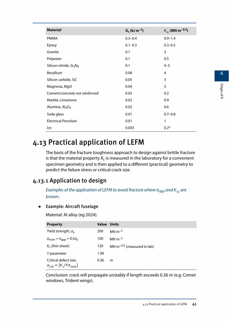
Material Gc (kJ m–2) KIc (MN m–3/2)
PMMA 0.3–0.4 0.9–1.4
Epoxy 0.1–0.3 0.3–0.5
Granite 0.1 3
Polyester 0.1 0.5
Silicon nitride, Si3N4 0.1 4–5
Beryllium 0.08 4
Silicon carbide, SiC 0.05 3
Magnesia, MgO 0.04 3
Cement/concrete not reinforced 0.03 0.2
Marble, Limestone 0.02 0.9
Alumina, Al2O3 0.02 0.6
Soda glass 0.01 0.7–0.8
Electrical Porcelain 0.01 1
Ice 0.003 0.2*
4.13 Practical application of LEFMThe basis of the fracture toughness approach to design against brittle fractureis that the material property Kc is measured in the laboratory for a convenientspecimen geometry and is then applied to a different (practical) geometry topredict the failure stress or critical crack size.
4.13.1 Application to designExamples of the application of LEFM to avoid fracture where σapp and KIc areknown.
● Example: Aircraft fuselage
Material: Al alloy (eg 2024).
Property Value Units
Yield strength, σy 200 MN m–2
σnom = σapp = 0.5σy 100 MN m–2
Kc (thin sheet) 120 MN m–3/2 (measured in lab)
Y parameter 1.99
Critical defect size,acrit = Kc/Yσnom
0.36 m
Conclusion: crack will propagate unstably if length exceeds 0.36 m (e.g. Cometwindows, Trident wings).
4
Origin of K
4.13 Practical application of LEFM 41
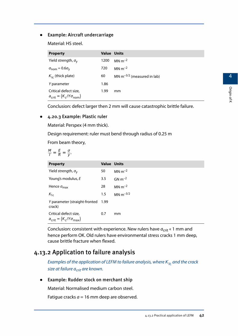
● Example: Aircraft undercarriage
Material: HS steel.
Property Value Units
Yield strength, σy 1200 MN m–2
σnom = 0.6σy 720 MN m–2
KIc (thick plate) 60 MN m–3/2 (measured in lab)
Y parameter 1.86
Critical defect size,acrit = Kc/Yσnom
1.99 mm
Conclusion: defect larger then 2 mm will cause catastrophic brittle failure.
● 4.20.3 Example: Plastic ruler
Material: Perspex (4 mm thick).
Design requirement: ruler must bend through radius of 0.25 m
From beam theory,
MI = E
R = σy .
Property Value Units
Yield strength, σy 50 MN m–2
Young’s modulus, E 3.5 GN m–2
Hence σmax 28 MN m–2
K1c 1.5 MN m–3/2
Y parameter (straight-frontedcrack)
1.99
Critical defect size,acrit = Kc/Yσmax
0.7 mm
Conclusion: consistent with experience. New rulers have acrit « 1 mm andhence perform OK. Old rulers have environmental stress cracks 1 mm deep,cause brittle fracture when flexed.
4.13.2 Application to failure analysisExamples of the application of LEFM to failure analysis, where KIc and the cracksize at failure acrit are known.
● Example: Rudder stock on merchant ship
Material: Normalised medium carbon steel.
Fatigue cracks a = 16 mm deep are observed.
4
Origin of K
4.13.2 Practical application of LEFM 42
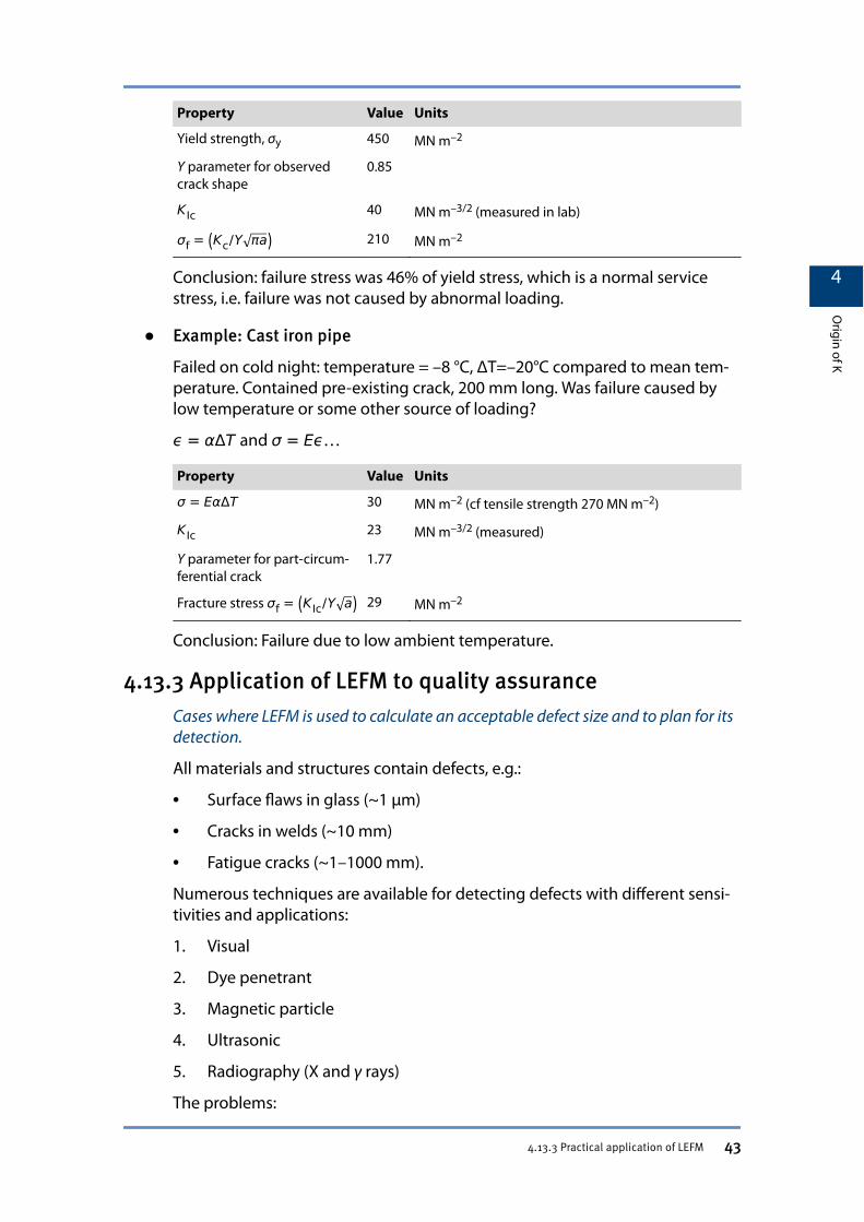
Property Value Units
Yield strength, σy 450 MN m–2
Y parameter for observedcrack shape
0.85
KIc 40 MN m–3/2 (measured in lab)
σf = Kc/Y πa 210 MN m–2
Conclusion: failure stress was 46% of yield stress, which is a normal servicestress, i.e. failure was not caused by abnormal loading.
● Example: Cast iron pipe
Failed on cold night: temperature = –8 °C, ΔT=–20°C compared to mean tem-perature. Contained pre-existing crack, 200 mm long. Was failure caused bylow temperature or some other source of loading?
ϵ = αΔT and σ = Eϵ…
Property Value Units
σ = EαΔT 30 MN m–2 (cf tensile strength 270 MN m–2)
KIc 23 MN m–3/2 (measured)
Y parameter for part-circum-ferential crack
1.77
Fracture stress σf = KIc/Y a 29 MN m–2
Conclusion: Failure due to low ambient temperature.
4.13.3 Application of LEFM to quality assuranceCases where LEFM is used to calculate an acceptable defect size and to plan for itsdetection.
All materials and structures contain defects, e.g.:
• Surface flaws in glass (~1 μm)
• Cracks in welds (~10 mm)
• Fatigue cracks (~1–1000 mm).
Numerous techniques are available for detecting defects with different sensi-tivities and applications:
1. Visual
2. Dye penetrant
3. Magnetic particle
4. Ultrasonic
5. Radiography (X and γ rays)
The problems:
4
Origin of K
4.13.3 Practical application of LEFM 43
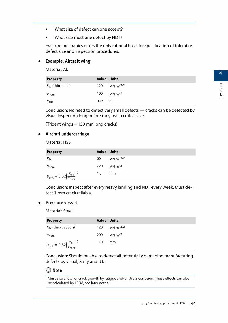
• What size of defect can one accept?
• What size must one detect by NDT?
Fracture mechanics offers the only rational basis for specification of tolerabledefect size and inspection procedures.
● Example: Aircraft wing
Material: Al.
Property Value Units
KIc (thin sheet) 120 MN m–3/2
σnom 100 MN m–2
acrit 0.46 m
Conclusion: No need to detect very small defects — cracks can be detected byvisual inspection long before they reach critical size.
(Trident wings = 150 mm long cracks).
● Aircraft undercarriage
Material: HSS.
Property Value Units
K1c 60 MN m–3/2
σnom 720 MN m–2
acrit = 0.32K1cσnom
2 1.8 mm
Conclusion: Inspect after every heavy landing and NDT every week. Must de-tect 1 mm crack reliably.
● Pressure vessel
Material: Steel.
Property Value Units
K1c (thick section) 120 MN m–3/2
σnom 200 MN m–2
acrit = 0.32K1cσnom
2 110 mm
Conclusion: Should be able to detect all potentially damaging manufacturingdefects by visual, X-ray and UT.
Note
Must also allow for crack growth by fatigue and/or stress corrosion. These effects can alsobe calculated by LEFM, see later notes.
4
Origin of K
4.13 Practical application of LEFM 44
4.14 The leak-before-break conceptA very important concept in the safe design of pressure vessels.
In the pressure vessel example above, acrit = 110 mm.
If wall thickness = 250 mm then acrit < t, i.e. if the crack remains undetectedand grows by fatigue, we will eventually get catastrophic brittle fracture — or,put another way, the vessel will explode.
Alternatively, by appropriate choice of steel toughness, stress and thickness,we can arrange that acrit = 300 mm. For example by increasing the fracturetoughness of the steel to >200 MN m–3/2 the critical crack length can be in-creased to over 300 mm.
Now if an undetected crack undergoes slow growth, it must penetrate the wallthickness before it can achieve a size sufficient for unstable fracture. But pene-tration of the wall will cause leakage of fluid which leads to a loss of pressurewhich in turn reduces the stress and lowers the driving force for failure. i.e. ves-sel leaks before it breaks.
4.15 Proof loadingThe traditional method of testing engineering components and structures.
Put simply, all that is done is to expose the component or structure to stress >service stress. If it survives it is then considered safe for service at the lowerstress.
Can get more information by analysing this process in terms of LEFM. For aservice stress σservice can calculate a critical defect size = acs.
If proof load to σproof and if the structure survives, then you know that no de-fects can be present greater than the critical defect size at σproof i.e. acp.
Now you know the margin of safety in terms of defect size and if necessarycan calculate the time for the defect to grow from the initial size to the criticaldefect size acs. This time then provides the basis for determining the subse-quent inspection intervals.
4
Origin of K
4.14 The leak-before-break concept 45
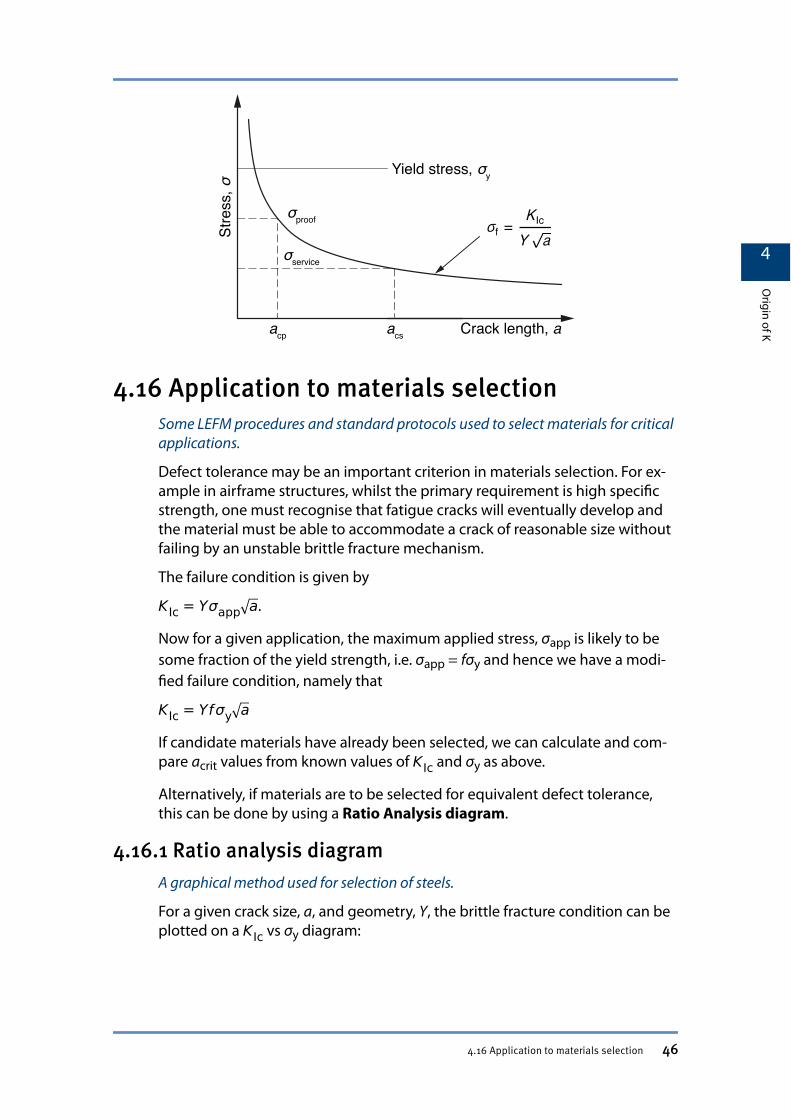
4.16 Application to materials selectionSome LEFM procedures and standard protocols used to select materials for criticalapplications.
Defect tolerance may be an important criterion in materials selection. For ex-ample in airframe structures, whilst the primary requirement is high specificstrength, one must recognise that fatigue cracks will eventually develop andthe material must be able to accommodate a crack of reasonable size withoutfailing by an unstable brittle fracture mechanism.
The failure condition is given by
KIc = Yσapp a.
Now for a given application, the maximum applied stress, σapp is likely to besome fraction of the yield strength, i.e. σapp = fσy and hence we have a modi-fied failure condition, namely that
KIc = Yfσy a
If candidate materials have already been selected, we can calculate and com-pare acrit values from known values of KIc and σy as above.
Alternatively, if materials are to be selected for equivalent defect tolerance,this can be done by using a Ratio Analysis diagram.
4.16.1 Ratio analysis diagramA graphical method used for selection of steels.
For a given crack size, a, and geometry, Y, the brittle fracture condition can beplotted on a KIc vs σy diagram:
4
Origin of K
4.16 Application to materials selection 46
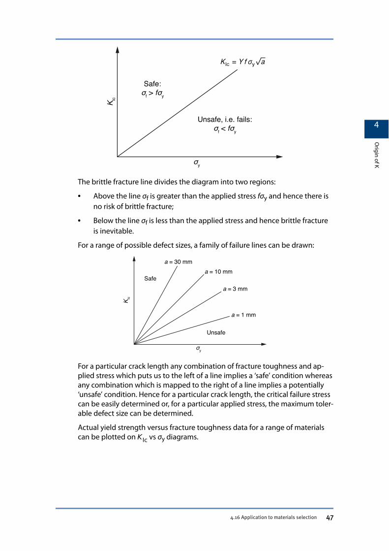
The brittle fracture line divides the diagram into two regions:
• Above the line σf is greater than the applied stress fσy and hence there isno risk of brittle fracture;
• Below the line σf is less than the applied stress and hence brittle fractureis inevitable.
For a range of possible defect sizes, a family of failure lines can be drawn:
For a particular crack length any combination of fracture toughness and ap-plied stress which puts us to the left of a line implies a ‘safe’ condition whereasany combination which is mapped to the right of a line implies a potentially‘unsafe’ condition. Hence for a particular crack length, the critical failure stresscan be easily determined or, for a particular applied stress, the maximum toler-able defect size can be determined.
Actual yield strength versus fracture toughness data for a range of materialscan be plotted on KIc vs σy diagrams.
4
Origin of K
4.16 Application to materials selection 47
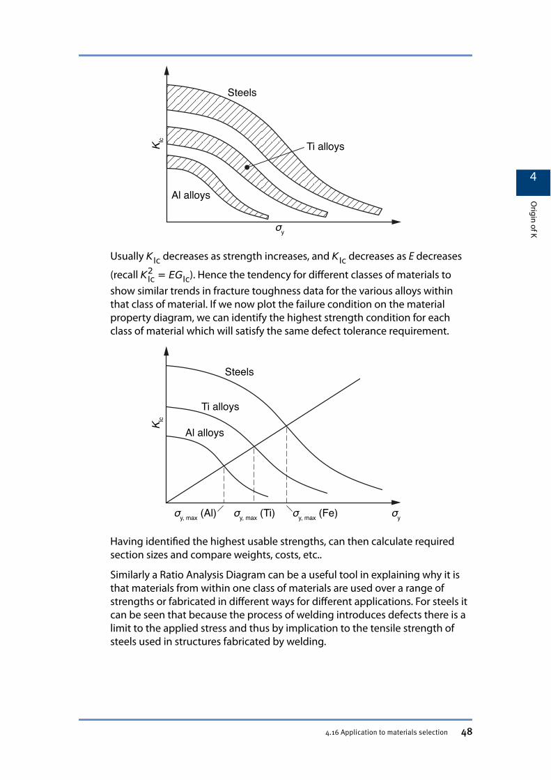
Usually KIc decreases as strength increases, and KIc decreases as E decreases
(recall KIc2 = EGIc). Hence the tendency for different classes of materials to
show similar trends in fracture toughness data for the various alloys withinthat class of material. If we now plot the failure condition on the materialproperty diagram, we can identify the highest strength condition for eachclass of material which will satisfy the same defect tolerance requirement.
Having identified the highest usable strengths, can then calculate requiredsection sizes and compare weights, costs, etc..
Similarly a Ratio Analysis Diagram can be a useful tool in explaining why it isthat materials from within one class of materials are used over a range ofstrengths or fabricated in different ways for different applications. For steels itcan be seen that because the process of welding introduces defects there is alimit to the applied stress and thus by implication to the tensile strength ofsteels used in structures fabricated by welding.
4
Origin of K
4.16 Application to materials selection 48
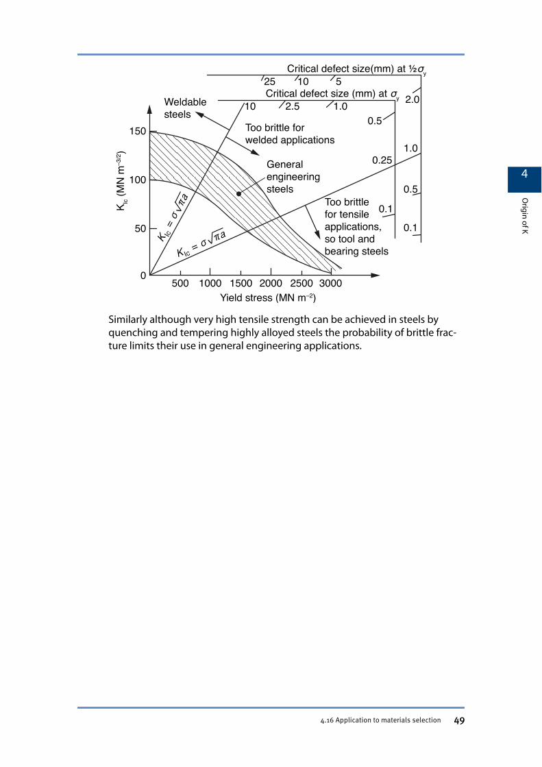
Similarly although very high tensile strength can be achieved in steels byquenching and tempering highly alloyed steels the probability of brittle frac-ture limits their use in general engineering applications.
4
Origin of K
4.16 Application to materials selection 49
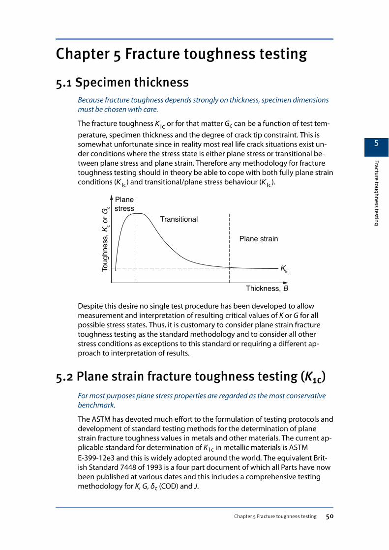
Chapter 5 Fracture toughness testing
5.1 Specimen thicknessBecause fracture toughness depends strongly on thickness, specimen dimensionsmust be chosen with care.
The fracture toughness KIc or for that matter Gc can be a function of test tem-perature, specimen thickness and the degree of crack tip constraint. This issomewhat unfortunate since in reality most real life crack situations exist un-der conditions where the stress state is either plane stress or transitional be-tween plane stress and plane strain. Therefore any methodology for fracturetoughness testing should in theory be able to cope with both fully plane strainconditions (KIc) and transitional/plane stress behaviour (KIc).
Despite this desire no single test procedure has been developed to allowmeasurement and interpretation of resulting critical values of K or G for allpossible stress states. Thus, it is customary to consider plane strain fracturetoughness testing as the standard methodology and to consider all otherstress conditions as exceptions to this standard or requiring a different ap-proach to interpretation of results.
5.2 Plane strain fracture toughness testing (K1c)For most purposes plane stress properties are regarded as the most conservativebenchmark.
The ASTM has devoted much effort to the formulation of testing protocols anddevelopment of standard testing methods for the determination of planestrain fracture toughness values in metals and other materials. The current ap-plicable standard for determination of K1c in metallic materials is ASTME-399-12e3 and this is widely adopted around the world. The equivalent Brit-ish Standard 7448 of 1993 is a four part document of which all Parts have nowbeen published at various dates and this includes a comprehensive testingmethodology for K, G, δc (COD) and J.
5
Fracture toughness testing
Chapter 5 Fracture toughness testing 50
All standardised fracture toughness protocols include the same elements,namely:
• A list of acceptable specimen geometries;
• Standard specimen preparation techniques;
• Standardised testing procedures; and
• A standardised method of determining K or G from the resulting test data.The fact that a particular specimen geometry does not appear in the list of ac-ceptable geometries in e.g. ASTM E-399-12e3 does not preclude its use as avalid means of determining fracture toughness for a particular specimen. Thespecimen geometries which do appear in the standards are those which havebeen found by extensive round-robin testing to give reproducable results indifferent laboratories within about 15%.
● Specimen Geometry
Acceptable specimen geometries are those for which the compliance calibra-tion curve as a function of normalised crack length is well documented andaccepted. Given that most practical or potential brittle fracture problems in-volve fairly large pieces of metal the ASTM and BS both include the CompactTension (CT) and Single Edged Notched Bend specimen (SENB) which will ca-ter for most available material configurations.
Since the test procedure requires that a sharp starter crack in the form of fati-gue crack is present in the specimen the standards also dictate the geometryof the starter notch from which the fatigue crack has to be initiated and grownto a required length. Specifying the geometry of the starter notch ensures thatthe fatigue crack initiates and remains in the mid-plane of the specimen andthat the crack front is symmetric.
● Specimen Size
Plane strain fracture toughness testing is almost unique in requiring that theexperimenter has a good idea of the result before carrying out the test! Sinceone of the main validity restriction for testing of this type is that fully planestrain conditions are developed at the crack tip the specimen must have cer-tain minimum dimensions.
Typical geometries which are or have been used for plane strain fracturetoughness determination are shown below together with their stress intensityfactor solutions and/or G solutions.
5.2.1 Centre cracked plate specimenGeometry and equations for determining K.
5
Fracture toughness testing
5.2.1 Plane strain fracture toughness testing (K1c) 51
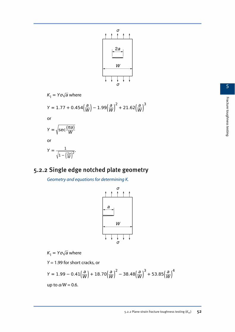
KI = Yσ a where
Y = 1.77 + 0.454 aW − 1.99 a
W2
+ 21.62 aW
3
or
Y = sec πaWor
Y = 11− 2a
W2 .
5.2.2 Single edge notched plate geometryGeometry and equations for determining K.
KI = Yσ a where
Y = 1.99 for short cracks, or
Y = 1.99− 0.41 aW + 18.70 a
W2− 38.48 a
W3
+ 53.85 aW
4
up to a/W = 0.6.
5
Fracture toughness testing
5.2.2 Plane strain fracture toughness testing (K1c) 52
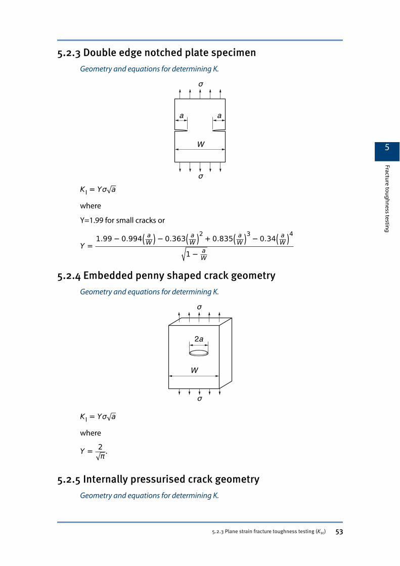
5.2.3 Double edge notched plate specimenGeometry and equations for determining K.
KI = Yσ a
where
Y=1.99 for small cracks or
Y =1.99− 0.994 a
W − 0.363 aW
2 + 0.835 aW
3− 0.34 aW
4
1− aW
5.2.4 Embedded penny shaped crack geometryGeometry and equations for determining K.
KI = Yσ a
where
Y = 2π .
5.2.5 Internally pressurised crack geometryGeometry and equations for determining K.
5
Fracture toughness testing
5.2.3 Plane strain fracture toughness testing (K1c) 53
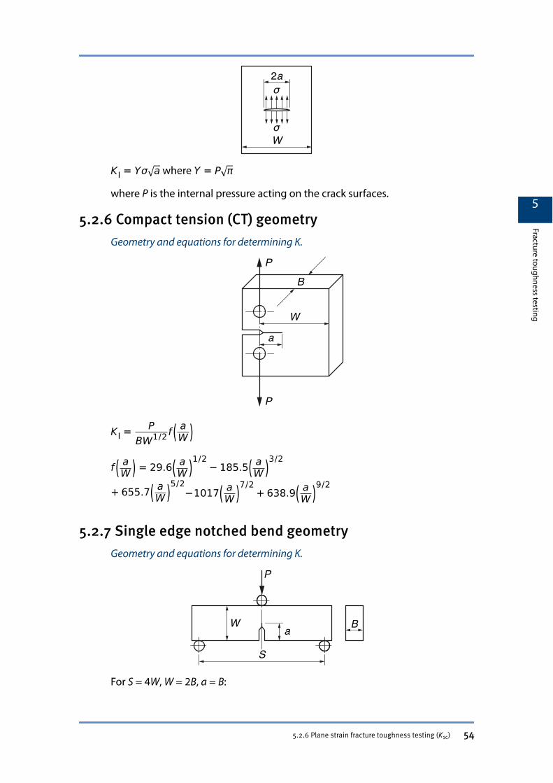
σ
σ
2a
W
KI = Yσ a where Y = P π
where P is the internal pressure acting on the crack surfaces.
5.2.6 Compact tension (CT) geometryGeometry and equations for determining K.
KI = PBW1/2 f
aW
f aW = 29.6 aW
1/2− 185.5 a
W3/2
+ 655.7 aW
5/2−1017 a
W7/2
+ 638.9 aW
9/2
5.2.7 Single edge notched bend geometryGeometry and equations for determining K.
For S = 4W, W = 2B, a = B:
5
Fracture toughness testing
5.2.6 Plane strain fracture toughness testing (K1c) 54
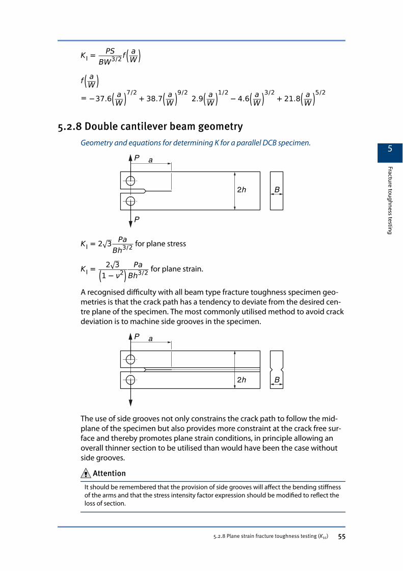
KI = PSBW3/2 f
aW
f aW
= −37.6 aW
7/2+ 38.7 a
W9/2
2.9 aW
1/2− 4.6 a
W3/2
+ 21.8 aW
5/2
5.2.8 Double cantilever beam geometryGeometry and equations for determining K for a parallel DCB specimen.
KI = 2 3 PaBh3/2 for plane stress
KI = 2 31− ν2
PaBh3/2 for plane strain.
A recognised difficulty with all beam type fracture toughness specimen geo-metries is that the crack path has a tendency to deviate from the desired cen-tre plane of the specimen. The most commonly utilised method to avoid crackdeviation is to machine side grooves in the specimen.
The use of side grooves not only constrains the crack path to follow the mid-plane of the specimen but also provides more constraint at the crack free sur-face and thereby promotes plane strain conditions, in principle allowing anoverall thinner section to be utilised than would have been the case withoutside grooves.
Attention
It should be remembered that the provision of side grooves will affect the bending stiffnessof the arms and that the stress intensity factor expression should be modified to reflect theloss of section.
5
Fracture toughness testing
5.2.8 Plane strain fracture toughness testing (K1c) 55
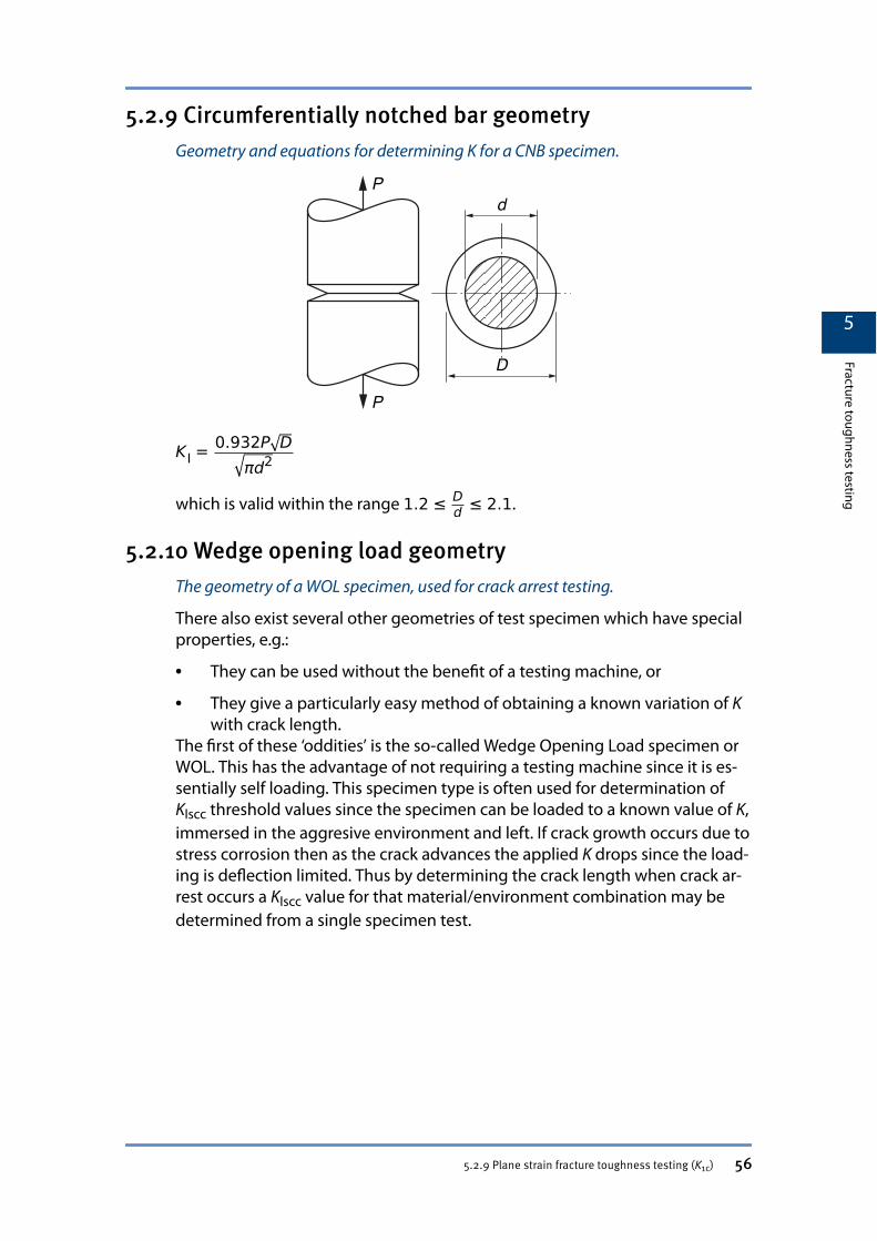
5.2.9 Circumferentially notched bar geometryGeometry and equations for determining K for a CNB specimen.
KI = 0.932P Dπd2
which is valid within the range 1.2 ≤ Dd ≤ 2.1.
5.2.10 Wedge opening load geometryThe geometry of a WOL specimen, used for crack arrest testing.
There also exist several other geometries of test specimen which have specialproperties, e.g.:
• They can be used without the benefit of a testing machine, or
• They give a particularly easy method of obtaining a known variation of Kwith crack length.
The first of these ‘oddities’ is the so-called Wedge Opening Load specimen orWOL. This has the advantage of not requiring a testing machine since it is es-sentially self loading. This specimen type is often used for determination ofKIscc threshold values since the specimen can be loaded to a known value of K,immersed in the aggresive environment and left. If crack growth occurs due tostress corrosion then as the crack advances the applied K drops since the load-ing is deflection limited. Thus by determining the crack length when crack ar-rest occurs a KIscc value for that material/environment combination may bedetermined from a single specimen test.
5
Fracture toughness testing
5.2.9 Plane strain fracture toughness testing (K1c) 56
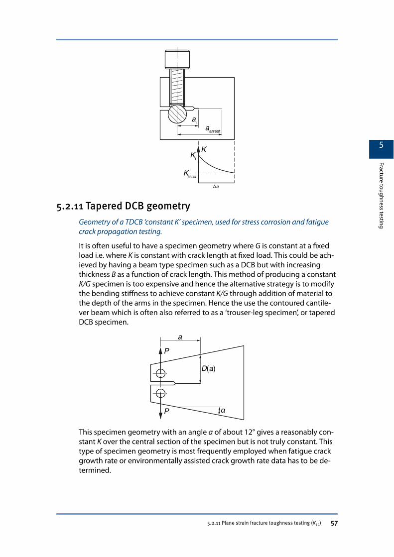
5.2.11 Tapered DCB geometryGeometry of a TDCB ‘constant K’ specimen, used for stress corrosion and fatiguecrack propagation testing.
It is often useful to have a specimen geometry where G is constant at a fixedload i.e. where K is constant with crack length at fixed load. This could be ach-ieved by having a beam type specimen such as a DCB but with increasingthickness B as a function of crack length. This method of producing a constantK/G specimen is too expensive and hence the alternative strategy is to modifythe bending stiffness to achieve constant K/G through addition of material tothe depth of the arms in the specimen. Hence the use the contoured cantile-ver beam which is often also referred to as a ‘trouser-leg specimen’, or taperedDCB specimen.
This specimen geometry with an angle α of about 12° gives a reasonably con-stant K over the central section of the specimen but is not truly constant. Thistype of specimen geometry is most frequently employed when fatigue crackgrowth rate or environmentally assisted crack growth rate data has to be de-termined.
5
Fracture toughness testing
5.2.11 Plane strain fracture toughness testing (K1c) 57
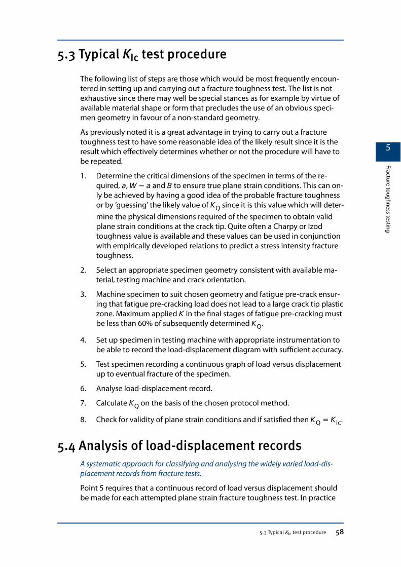
5.3 Typical KIc test procedure
The following list of steps are those which would be most frequently encoun-tered in setting up and carrying out a fracture toughness test. The list is notexhaustive since there may well be special stances as for example by virtue ofavailable material shape or form that precludes the use of an obvious speci-men geometry in favour of a non-standard geometry.
As previously noted it is a great advantage in trying to carry out a fracturetoughness test to have some reasonable idea of the likely result since it is theresult which effectively determines whether or not the procedure will have tobe repeated.
1. Determine the critical dimensions of the specimen in terms of the re-quired, a, W − a and B to ensure true plane strain conditions. This can on-ly be achieved by having a good idea of the probable fracture toughnessor by ‘guessing’ the likely value of KQ since it is this value which will deter-mine the physical dimensions required of the specimen to obtain validplane strain conditions at the crack tip. Quite often a Charpy or Izodtoughness value is available and these values can be used in conjunctionwith empirically developed relations to predict a stress intensity fracturetoughness.
2. Select an appropriate specimen geometry consistent with available ma-terial, testing machine and crack orientation.
3. Machine specimen to suit chosen geometry and fatigue pre-crack ensur-ing that fatigue pre-cracking load does not lead to a large crack tip plasticzone. Maximum applied K in the final stages of fatigue pre-cracking mustbe less than 60% of subsequently determined KQ.
4. Set up specimen in testing machine with appropriate instrumentation tobe able to record the load-displacement diagram with sufficient accuracy.
5. Test specimen recording a continuous graph of load versus displacementup to eventual fracture of the specimen.
6. Analyse load-displacement record.
7. Calculate KQ on the basis of the chosen protocol method.
8. Check for validity of plane strain conditions and if satisfied then KQ = KIc.
5.4 Analysis of load-displacement recordsA systematic approach for classifying and analysing the widely varied load-dis-placement records from fracture tests.
Point 5 requires that a continuous record of load versus displacement shouldbe made for each attempted plane strain fracture toughness test. In practice
5
Fracture toughness testing
5.3 Typical KIc test procedure 58
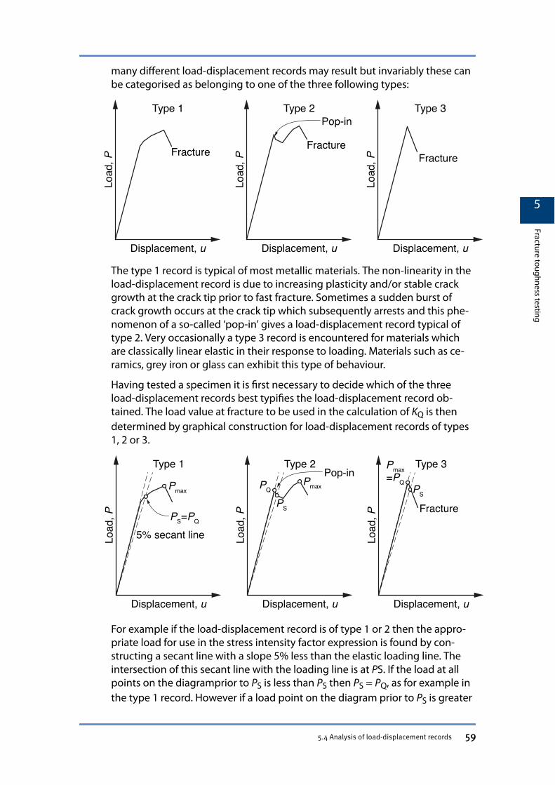
many different load-displacement records may result but invariably these canbe categorised as belonging to one of the three following types:
The type 1 record is typical of most metallic materials. The non-linearity in theload-displacement record is due to increasing plasticity and/or stable crackgrowth at the crack tip prior to fast fracture. Sometimes a sudden burst ofcrack growth occurs at the crack tip which subsequently arrests and this phe-nomenon of a so-called ‘pop-in’ gives a load-displacement record typical oftype 2. Very occasionally a type 3 record is encountered for materials whichare classically linear elastic in their response to loading. Materials such as ce-ramics, grey iron or glass can exhibit this type of behaviour.
Having tested a specimen it is first necessary to decide which of the threeload-displacement records best typifies the load-displacement record ob-tained. The load value at fracture to be used in the calculation of KQ is thendetermined by graphical construction for load-displacement records of types1, 2 or 3.
For example if the load-displacement record is of type 1 or 2 then the appro-priate load for use in the stress intensity factor expression is found by con-structing a secant line with a slope 5% less than the elastic loading line. Theintersection of this secant line with the loading line is at PS. If the load at allpoints on the diagramprior to PS is less than PS then PS = PQ, as for example inthe type 1 record. However if a load point on the diagram prior to PS is greater
5
Fracture toughness testing
5.4 Analysis of load-displacement records 59
than PS then the appropriate load for calculation of KQ is the maximum loadpreceding PS, as for example in type 2.
There is a additional, necessary restriction in that for both types 1 and 2 the
maximum load PmaxPQ
≤ 1.10 this restriction being intended to ensure that too
much stable crack growth has not occurred prior to fracture.
If PmaxPQ
≥ 1.10 the test must either be repeated with a thicker specimen or the
use of a plane strain fracture toughness protocol is inappropriate in whichcase a KIc approach to interpretation of the record should be adopted or analternative measure of fracture toughness should be adopted. Where the load-displacement record conforms to type 3 then the maximum load recorded isthe appropriate value to be used in calculating the provisional fracture tough-ness values.
Further restrictions apply to the shape of the crack front at the onset of brittlefracture which must be reasonably straight fronted to conform to the standardand if these restrictions are satisfied then the deduced value of stress intensityfactor at fracture, KQ is tested to ensure plane strain conditions.
If the dimensions of the specimen tested were such that:
B,W − a,a ≥ 2.5KQσy
2
then KQ = KIc and the value of stress intensity at brittle fracture is the planestrain fracture toughness which can be regarded as a material property in thesame way as yield stress or tensile strength. In practice at least two specimensof the same geometry would be tested and the results should be within 5 to10% for a satisfactory result to be recorded.
5.5 Plane stress fracture toughness (Kc) testingMethods for testing materials when plane strain conditions are inappropriate orpractically unattainable.
5.5.1 Plane stress regionIn this region, toughness increases rapidly with thickness.
In order to describe an appropriate method for non-plane strain fracturetoughness testing reference must again be made to the general toughnessversus thickness relationship for metals.
5
Fracture toughness testing
5.5 Plane stress fracture toughness (Kc) testing 60
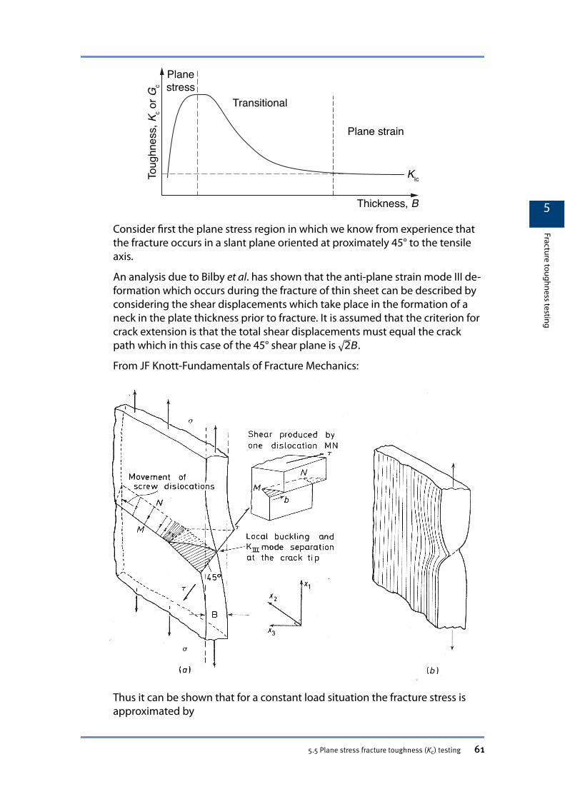
Consider first the plane stress region in which we know from experience thatthe fracture occurs in a slant plane oriented at proximately 45° to the tensileaxis.
An analysis due to Bilby et al. has shown that the anti-plane strain mode III de-formation which occurs during the fracture of thin sheet can be described byconsidering the shear displacements which take place in the formation of aneck in the plate thickness prior to fracture. It is assumed that the criterion forcrack extension is that the total shear displacements must equal the crackpath which in this case of the 45° shear plane is 2B.
From JF Knott-Fundamentals of Fracture Mechanics:
Thus it can be shown that for a constant load situation the fracture stress isapproximated by
5
Fracture toughness testing
5.5 Plane stress fracture toughness (Kc) testing 61
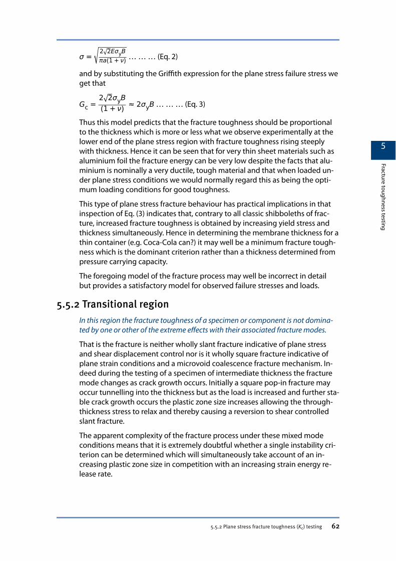
σ =2 2EσyBπa 1 + ν … … … (Eq. 2)
and by substituting the Griffith expression for the plane stress failure stress weget that
Gc =2 2σyB1 + ν ≈ 2σyB … … … (Eq. 3)
Thus this model predicts that the fracture toughness should be proportionalto the thickness which is more or less what we observe experimentally at thelower end of the plane stress region with fracture toughness rising steeplywith thickness. Hence it can be seen that for very thin sheet materials such asaluminium foil the fracture energy can be very low despite the facts that alu-minium is nominally a very ductile, tough material and that when loaded un-der plane stress conditions we would normally regard this as being the opti-mum loading conditions for good toughness.
This type of plane stress fracture behaviour has practical implications in thatinspection of Eq. (3) indicates that, contrary to all classic shibboleths of frac-ture, increased fracture toughness is obtained by increasing yield stress andthickness simultaneously. Hence in determining the membrane thickness for athin container (e.g. Coca-Cola can?) it may well be a minimum fracture tough-ness which is the dominant criterion rather than a thickness determined frompressure carrying capacity.
The foregoing model of the fracture process may well be incorrect in detailbut provides a satisfactory model for observed failure stresses and loads.
5.5.2 Transitional regionIn this region the fracture toughness of a specimen or component is not domina-ted by one or other of the extreme effects with their associated fracture modes.
That is the fracture is neither wholly slant fracture indicative of plane stressand shear displacement control nor is it wholly square fracture indicative ofplane strain conditions and a microvoid coalescence fracture mechanism. In-deed during the testing of a specimen of intermediate thickness the fracturemode changes as crack growth occurs. Initially a square pop-in fracture mayoccur tunnelling into the thickness but as the load is increased and further sta-ble crack growth occurs the plastic zone size increases allowing the through-thickness stress to relax and thereby causing a reversion to shear controlledslant fracture.
The apparent complexity of the fracture process under these mixed modeconditions means that it is extremely doubtful whether a single instability cri-terion can be determined which will simultaneously take account of an in-creasing plastic zone size in competition with an increasing strain energy re-lease rate.
5
Fracture toughness testing
5.5.2 Plane stress fracture toughness (Kc) testing 62
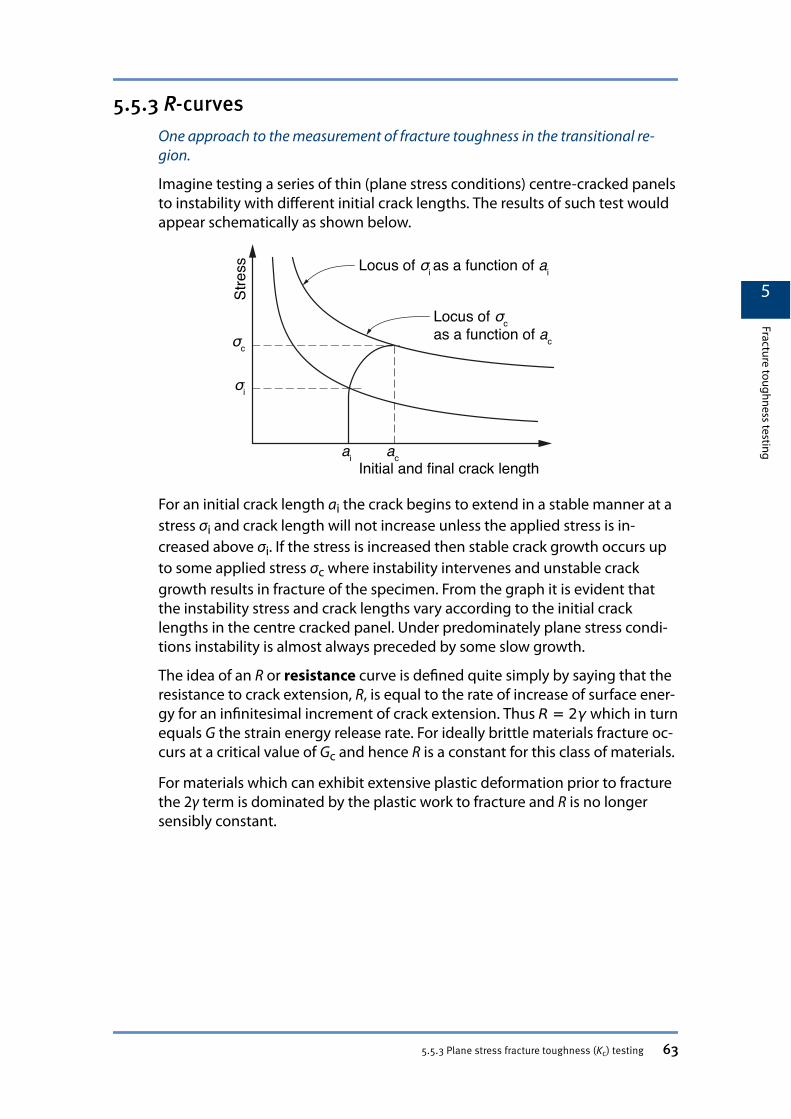
5.5.3 R-curvesOne approach to the measurement of fracture toughness in the transitional re-gion.
Imagine testing a series of thin (plane stress conditions) centre-cracked panelsto instability with different initial crack lengths. The results of such test wouldappear schematically as shown below.
For an initial crack length ai the crack begins to extend in a stable manner at astress σi and crack length will not increase unless the applied stress is in-creased above σi. If the stress is increased then stable crack growth occurs upto some applied stress σc where instability intervenes and unstable crackgrowth results in fracture of the specimen. From the graph it is evident thatthe instability stress and crack lengths vary according to the initial cracklengths in the centre cracked panel. Under predominately plane stress condi-tions instability is almost always preceded by some slow growth.
The idea of an R or resistance curve is defined quite simply by saying that theresistance to crack extension, R, is equal to the rate of increase of surface ener-gy for an infinitesimal increment of crack extension. Thus R = 2γ which in turnequals G the strain energy release rate. For ideally brittle materials fracture oc-curs at a critical value of Gc and hence R is a constant for this class of materials.
For materials which can exhibit extensive plastic deformation prior to fracturethe 2γ term is dominated by the plastic work to fracture and R is no longersensibly constant.
5
Fracture toughness testing
5.5.3 Plane stress fracture toughness (Kc) testing 63
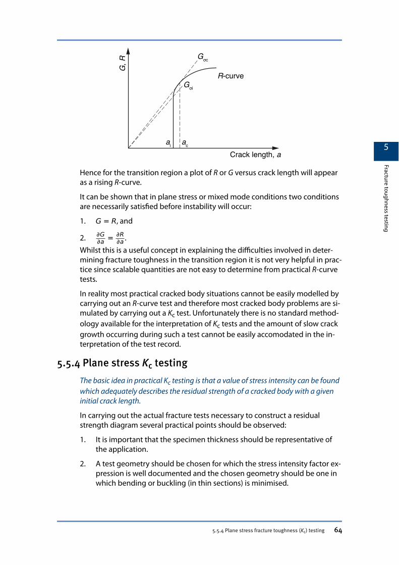
Hence for the transition region a plot of R or G versus crack length will appearas a rising R-curve.
It can be shown that in plane stress or mixed mode conditions two conditionsare necessarily satisfied before instability will occur:
1. G = R, and
2. ∂G∂a = ∂R
∂a .
Whilst this is a useful concept in explaining the difficulties involved in deter-mining fracture toughness in the transition region it is not very helpful in prac-tice since scalable quantities are not easy to determine from practical R-curvetests.
In reality most practical cracked body situations cannot be easily modelled bycarrying out an R-curve test and therefore most cracked body problems are si-mulated by carrying out a Kc test. Unfortunately there is no standard method-ology available for the interpretation of Kc tests and the amount of slow crackgrowth occurring during such a test cannot be easily accomodated in the in-terpretation of the test record.
5.5.4 Plane stress Kc testingThe basic idea in practical Kc testing is that a value of stress intensity can be foundwhich adequately describes the residual strength of a cracked body with a giveninitial crack length.
In carrying out the actual fracture tests necessary to construct a residualstrength diagram several practical points should be observed:
1. It is important that the specimen thickness should be representative ofthe application.
2. A test geometry should be chosen for which the stress intensity factor ex-pression is well documented and the chosen geometry should be one inwhich bending or buckling (in thin sections) is minimised.
5
Fracture toughness testing
5.5.4 Plane stress fracture toughness (Kc) testing 64
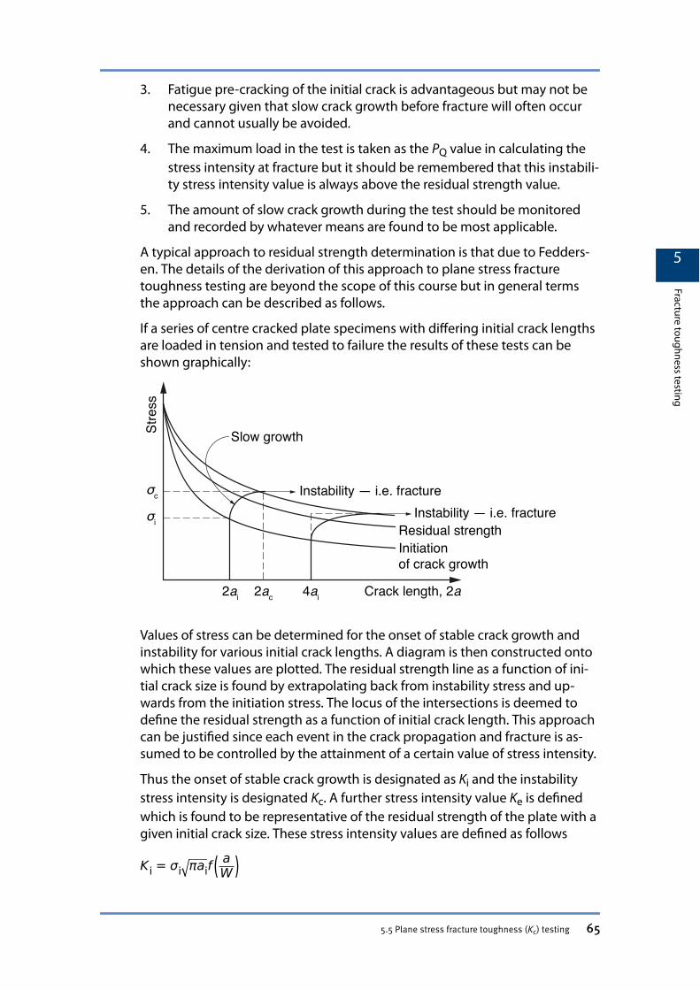
3. Fatigue pre-cracking of the initial crack is advantageous but may not benecessary given that slow crack growth before fracture will often occurand cannot usually be avoided.
4. The maximum load in the test is taken as the PQ value in calculating thestress intensity at fracture but it should be remembered that this instabili-ty stress intensity value is always above the residual strength value.
5. The amount of slow crack growth during the test should be monitoredand recorded by whatever means are found to be most applicable.
A typical approach to residual strength determination is that due to Fedders-en. The details of the derivation of this approach to plane stress fracturetoughness testing are beyond the scope of this course but in general termsthe approach can be described as follows.
If a series of centre cracked plate specimens with differing initial crack lengthsare loaded in tension and tested to failure the results of these tests can beshown graphically:
Values of stress can be determined for the onset of stable crack growth andinstability for various initial crack lengths. A diagram is then constructed ontowhich these values are plotted. The residual strength line as a function of ini-tial crack size is found by extrapolating back from instability stress and up-wards from the initiation stress. The locus of the intersections is deemed todefine the residual strength as a function of initial crack length. This approachcan be justified since each event in the crack propagation and fracture is as-sumed to be controlled by the attainment of a certain value of stress intensity.
Thus the onset of stable crack growth is designated as Ki and the instabilitystress intensity is designated Kc. A further stress intensity value Ke is definedwhich is found to be representative of the residual strength of the plate with agiven initial crack size. These stress intensity values are defined as follows
Ki = σi πaifaW
5
Fracture toughness testing
5.5 Plane stress fracture toughness (Kc) testing 65
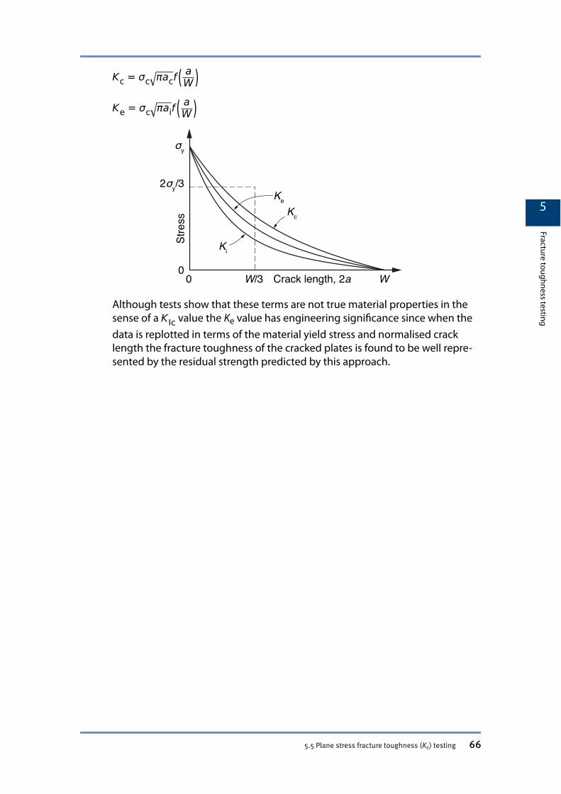
Kc = σc πacfaW
Ke = σc πaifaW
Although tests show that these terms are not true material properties in thesense of a KIc value the Ke value has engineering significance since when thedata is replotted in terms of the material yield stress and normalised cracklength the fracture toughness of the cracked plates is found to be well repre-sented by the residual strength predicted by this approach.
5
Fracture toughness testing
5.5 Plane stress fracture toughness (Kc) testing 66
Chapter 6 Crack opening displacement(COD)
A method of characterising failures which can be classified as ‘fracture’ but are tooductile for LEFM.
The previous parts of this course discussed methods and applications for pre-dicting the onset of fracture in situations where the risk of crack propagationwithout appreciable amounts of plastic behaviour exists. In this situation engi-neering brittle fracture occurs (“breaks before it bends”) and this is a phenom-enon that can be accurately described using LEFM. The fracture criterion de-veloped for the brittle fracture situation requires that:
1. A material property (KIc) can measured for the material in question;
2. The applied stress intensity severity on the cracked component can becalculated from a knowledge of the shape factors plus load and cracklength; and
3. The likelihood of fracture can be assessed by comparing the two.Two situations may arise in which the use of the LEFM parameters becomesimpossible.
1. Problems in measuring the material property. For some materials, theminimum thickness necessary to measure a valid KIc can make the testimpossible to perform either through difficulties with the size of rig re-quired, or due to material being unavailable in the required thicknessrange.
2. Problems arising from the applied stress intensity on the cracked compo-nent. There are situations in which the amount of plasticity near the cracktip invalidates the use of the LEFM approach to describe the applied se-verity.
This section describes a method of characterising failures that can occur bycracking with considerably less overall ductility than expected from a conven-tional tensile test, but with yielding extensive enough to make LEFM inappli-cable. These situations arise typically for structural steels and aluminium alloysof moderate strength, and define the intended scope of Elastic Plastic FractureMechanics (EPFM).
The formal scheme for EPFM follows that of LEFM, in that an attempt is madeto define a single parameter that measures the intensity of the deformationsapplied to a sharp crack. This time, however, the presence of plasticity is ac-knowledged rather than neglected. The material response is measured no-tionally by some critical value of that chosen parameter. So far, two such pa-rameters have emerged:
1. The so-called J-contour integral; and
2. The critical value of crack opening displacement, COD.
6
Crack opening displacement (CO
D)
Chapter 6 Crack opening displacement (COD) 67
The following sections describe approaches used to tackle the problem offracture toughness testing in the presence of plasticity. Initially the plasticzone size correction is discussed as the first attempt to extend LEFM consider-ations and include plasticity effects. Then the crack opening displacementmethod is described in detail and the idea of a fracture assessment diagram(FAD) is introduced in very general terms.
6.1 The plastic zone correctionWhen plasticity which is restricted to a zone near the crack tip, a small adjustmentto LEFM is sufficient.
The problem of determining the size or extent of the plastic zone ahead of acrack is a very complex one. This is due not only to the non-linearity of theplasticity constitutive equations, but also to the incremental nature of plastici-ty. Instead of attempting to completely describe the plastic zone in terms ofshape and extent, a useful simplification is to assume a shape and, given thatshape, to calculate the extent (i.e. a plastic zone size).
As a first attempt to account for plasticity we consider that a small plastic zoneexists ahead of the crack tip and that the global effect of such a zone is tomake the cracked body more compliant (less stiff). This is equivalent to theeffect of having a longer crack. A tentative description of the effect is thenmade by using a virtual, longer crack length. The plastic zone is roughly quan-tified by considering the point where σyy = σy. The value of r for which thathappens is taken as the radius rp of a small plastic zone. From the LEFM stresssolutions this corresponds to:
r = 12π
K2
σy2 = rp … … … (Eq. 1)
and the existing elastic analysis is retained for an effective crack of 2(a + rp)instead of 2a.
Since the whole solution is for elastic situations, only small plastic zones areacceptable and this is good enough for a first order correction factor. The finalresult is a measured G or K which is higher than the pure LEFM one, in agree-ment with the increase in fracture toughness expected due to plastic behav-iour.
However it should be self evident that for larger amounts of yielding the argu-ment does not hold.
6.2 Crack opening displacementCOD can be used to characterise fracture where plastic flow is no longer smallscale, but is restricted to the crack plane.
The concept of crack opening displacement, COD, was introduced in the UK byWells in 1961. Wells argued that, due to the plastic response of a material, the
6
Crack opening displacement (CO
D)
6.1 The plastic zone correction 68
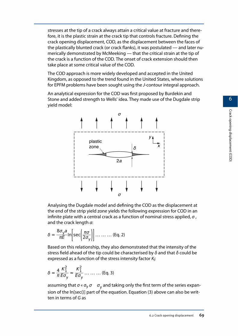
stresses at the tip of a crack always attain a critical value at fracture and there-fore, it is the plastic strain at the crack tip that controls fracture. Defining thecrack opening displacement, COD, as the displacement between the faces ofthe plastically blunted crack (or crack flanks), it was postulated — and later nu-merically demonstrated by McMeeking — that the critical strain at the tip ofthe crack is a function of the COD. The onset of crack extension should thentake place at some critical value of the COD.
The COD approach is more widely developed and accepted in the UnitedKingdom, as opposed to the trend found in the United States, where solutionsfor EPFM problems have been sought using the J-contour integral approach.
An analytical expression for the COD was first proposed by Burdekin andStone and added strength to Wells’ idea. They made use of the Dugdale stripyield model:
Analysing the Dugdale model and defining the COD as the displacement atthe end of the strip yield zone yields the following expression for COD in aninfinite plate with a central crack as a function of nominal stress applied, σ ,and the crack length a:
δ =8σyaπE ln sec πσ
2σy … … … (Eq. 2)
Based on this relationship, they also demonstrated that the intensity of thestress field ahead of the tip could be characterised by δ and that δ could beexpressed as a function of the stress intensity factor KI:
δ = 4πK1
2
Eσy≈K1
2
Eσy … … … (Eq. 3)
assuming that σ « σy σ σy and taking only the first term of the series expan-sion of the ln[sec()] part of the equation. Equation (3) above can also be writ-ten in terms of G as
6
Crack opening displacement (CO
D)
6.2 Crack opening displacement 69
δ = Gσy
… … … (Eq. 4)
within the assumptions of the strip yield model, namely for a state of planestress and for a non-work hardening material. The equation can be rewrittento describe a wider group of materials as
δ = Gmσy
… … … (Eq. 5)
where m is a factor representative of a material for a particular level of con-straint (thickness) and takes values between 1.0 for plane stress and about 2.0for plane strain.
In spite of being restricted to the geometry for which it was developed —wide plate, centre crack — this relationship shows that, in the elastic regime,the COD approach is in accordance with the LEFM predictions. In addition tothis, the COD approach is not intrinsically incompatible with situations beyondlinear elastic limits, as LEFM is, because the occurrence of crack tip plasticity ispart of the model itself.
When using COD in design it is usual to express the COD in a non-dimensionalform φ:
ϕ = δ2πϵya
… … … (Eq. 6),
where a is the crack length and ϵy is the strain at yield (as in σy/E). The use ofthe COD parameter in design is discussed in a later section. The underlyingidea is that the critical value of COD is a fundamental quantity that can betransferred from the test piece on to the real structure and characterises fail-ure even in the presence of plasticity.
The basis of the COD approach to toughness characterisation is that the localprocesses resulting in separation at the crack tip are identical in the nominallyelastic and yielding situations (provided full thickness of material is em-ployed). If this is so, the critical COD, δc should be a characteristic of the mate-rial and the state of stress at the crack tip (i.e. δc is thickness dependent in thesame way as KIc). Hence δc should characterise toughness in a similar mannerto KIc or Gc.
6
Crack opening displacement (CO
D)
6.2 Crack opening displacement 70
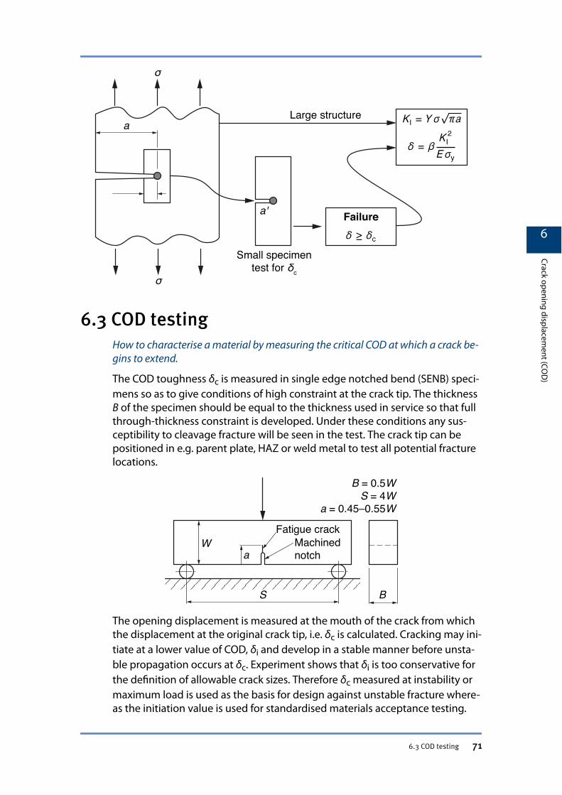
6.3 COD testingHow to characterise a material by measuring the critical COD at which a crack be-gins to extend.
The COD toughness δc is measured in single edge notched bend (SENB) speci-mens so as to give conditions of high constraint at the crack tip. The thicknessB of the specimen should be equal to the thickness used in service so that fullthrough-thickness constraint is developed. Under these conditions any sus-ceptibility to cleavage fracture will be seen in the test. The crack tip can bepositioned in e.g. parent plate, HAZ or weld metal to test all potential fracturelocations.
The opening displacement is measured at the mouth of the crack from whichthe displacement at the original crack tip, i.e. δc is calculated. Cracking may ini-tiate at a lower value of COD, δi and develop in a stable manner before unsta-ble propagation occurs at δc. Experiment shows that δi is too conservative forthe definition of allowable crack sizes. Therefore δc measured at instability ormaximum load is used as the basis for design against unstable fracture where-as the initiation value is used for standardised materials acceptance testing.
6
Crack opening displacement (CO
D)
6.3 COD testing 71
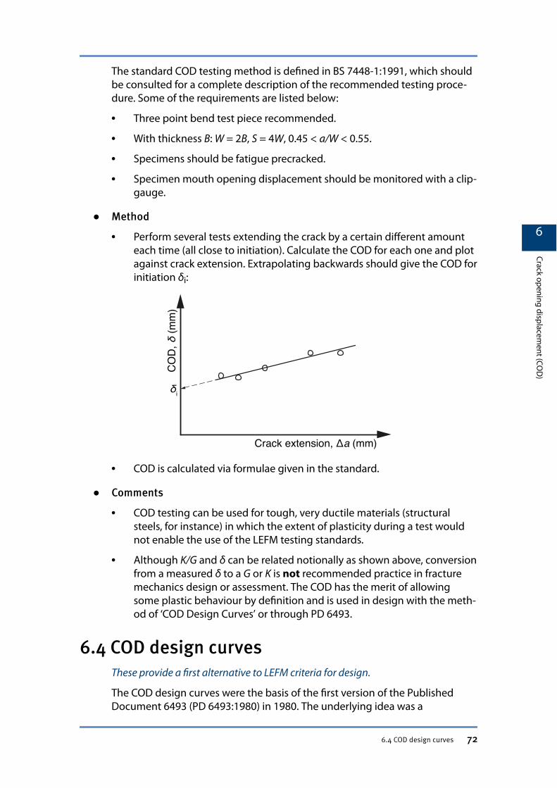
The standard COD testing method is defined in BS 7448-1:1991, which shouldbe consulted for a complete description of the recommended testing proce-dure. Some of the requirements are listed below:
• Three point bend test piece recommended.
• With thickness B: W = 2B, S = 4W, 0.45 < a/W < 0.55.
• Specimens should be fatigue precracked.
• Specimen mouth opening displacement should be monitored with a clip-gauge.
● Method
• Perform several tests extending the crack by a certain different amounteach time (all close to initiation). Calculate the COD for each one and plotagainst crack extension. Extrapolating backwards should give the COD forinitiation δi:
• COD is calculated via formulae given in the standard.
● Comments
• COD testing can be used for tough, very ductile materials (structuralsteels, for instance) in which the extent of plasticity during a test wouldnot enable the use of the LEFM testing standards.
• Although K/G and δ can be related notionally as shown above, conversionfrom a measured δ to a G or K is not recommended practice in fracturemechanics design or assessment. The COD has the merit of allowingsome plastic behaviour by definition and is used in design with the meth-od of ‘COD Design Curves’ or through PD 6493.
6.4 COD design curvesThese provide a first alternative to LEFM criteria for design.
The COD design curves were the basis of the first version of the PublishedDocument 6493 (PD 6493:1980) in 1980. The underlying idea was a
6
Crack opening displacement (CO
D)
6.4 COD design curves 72
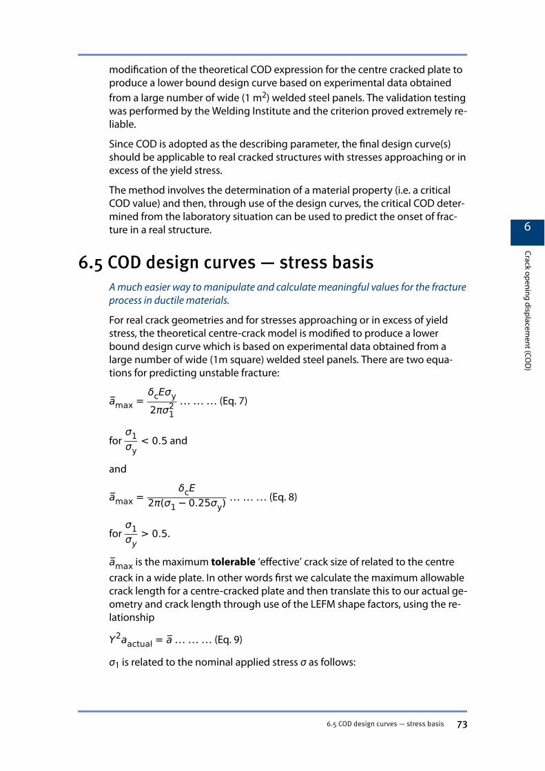
modification of the theoretical COD expression for the centre cracked plate toproduce a lower bound design curve based on experimental data obtainedfrom a large number of wide (1 m2) welded steel panels. The validation testingwas performed by the Welding Institute and the criterion proved extremely re-liable.
Since COD is adopted as the describing parameter, the final design curve(s)should be applicable to real cracked structures with stresses approaching or inexcess of the yield stress.
The method involves the determination of a material property (i.e. a criticalCOD value) and then, through use of the design curves, the critical COD deter-mined from the laboratory situation can be used to predict the onset of frac-ture in a real structure.
6.5 COD design curves — stress basisA much easier way to manipulate and calculate meaningful values for the fractureprocess in ductile materials.
For real crack geometries and for stresses approaching or in excess of yieldstress, the theoretical centre-crack model is modified to produce a lowerbound design curve which is based on experimental data obtained from alarge number of wide (1m square) welded steel panels. There are two equa-tions for predicting unstable fracture:
amax =δcEσy2πσ1
2 … … … (Eq. 7)
for σ1σy
< 0.5 and
and
amax =δcE
2π(σ1− 0.25σy) … … … (Eq. 8)
for σ1σy
> 0.5.
amax is the maximum tolerable ‘effective’ crack size of related to the centrecrack in a wide plate. In other words first we calculate the maximum allowablecrack length for a centre-cracked plate and then translate this to our actual ge-ometry and crack length through use of the LEFM shape factors, using the re-lationship
Y2aactual = a … … … (Eq. 9)
σ1 is related to the nominal applied stress σ as follows:
6
Crack opening displacement (CO
D)
6.5 COD design curves — stress basis 73
Location of crack Weld condition Magnitude of σ1
Remote from stress Stress relieved σ
As-welded σ + σy
At site of stress concentration SCF = kt Stress relieved ktσ
As-welded ktσ + σy
Note
It is possible that σ1 > σy even for plane stress situations. This arises because the COD ap-proach should properly be formulated in terms of strain rather than stress, i.e. σ1 and σyshould be replaced by ϵy and ϵy in the above equations. There is no problem in having ϵygreater ϵy. Usually it is more convenient to use the equations in terms of the equivalent no-tionally elastic stresses.
The design curve is intended to be deliberately conservative. Calculated tol-erable defect sizes are typically a factor of 2 smaller than the actual criticaldefect size. This arises because the use of the Dugdale model assumes planestress conditions which means that yielding is assumed to occur when theequivalent stress reaches σy. In reality most structures will require a higherequivalent stress to be achieved before yielding can occur, because of con-straint. Thus the actual COD will be less than predicted by the design curvewith a commensurately smaller tolerable crack size being predicted.
6.6 COD design curves — strain basisThe origin of the correlation between mouth opening and fracture toughness wasbased originally on strains.
As noted above the original and fundamental derivation of COD was formula-ted in terms of strains. For the sake of completeness it is worth runningthrough the same procedures as in §6.6, but using the non- dimensionalisedform of the COD :
ϕ =δc
2πϵya … … … (Eq. 10)
where ϵy is the strain at yield and a is related to the real crack length by
Important
a = Y2a (when K = Yσ πa) ——— (Eq. 9 again)
In other words an effective crack length is determined from Eq. (9) through theuse of the normal geometry factors which would be appropriate for the crackgeometry and length in the body in the LEFM situation.
The non-dimensional COD is then related to nominal strain, ε, in the absenceof the crack by
ϕ = ϵϵy
2 for ϵϵy
≤ 0.5
6
Crack opening displacement (CO
D)
6.6 COD design curves — strain basis 74
and
ϕ = ϵϵy− 0.25 for ϵϵy
≥ 0.5 … … … (Eq. 11).
• The value of ϵ/ϵy is estimated from nominal elastic theory in the absenceof a crack, i.e. -
• for no stress concentration, ϵ = σ/E;
• for SCF = kt, ϵ = ktσ/E;if the value of ϵ/ϵy exceeds 2, then a more accurate estimate of the strainsis necessary (e.g. by finite element computation).
• If residual stresses exist, as for example in non-stress relieved weldments,the residual stress term, σr , is added if known or must assumed to beequal to the yield stress. In which case
• ϵ = 1E σr + Ktσ .
Thus for a given problem the strain ϵ in the structure is estimated and φ evalu-ated. Either the required material toughness or the critical crack size can becalculated from the relationships above in precisely the same manner as forthe stress based method.
As previously stated the COD design curve is intended to be deliberately con-servative. Calculated tolerable defect sizes are typically a factor of 2 smallerthan the critical defect size. This conservatism is inherent in the formulation ofthe design curves from experimental data. However the COD method is argua-bly the best method for characterising weld metal toughness and several in-ternationally accepted welding standards specify COD testing for quality con-trol in the production of welded structures. In particular the production of thelarge welded jackets for North Sea oil rigs and the associated welded steelpipelines are all controlled through the specification of a minimum value of δcto be attained in the HAZ, weld metal and parent metal.
6.7 The Failure Assessment Diagram conceptFor assessment of a given structure under extreme loading conditions, aFAD helps determine whether EPFM or plastic collapse is the dominantmechanism.
The boundary between EPFM and general yielding is subtle and loosely de-fined. In practice this means that structures loaded close to generalised yieldloads should have a fracture assessment performed in conjunction with a plas-tic collapse assessment.
The concept of the failure assessment diagram (FAD) is so far the best solutionto this problem. A failure assessment diagram is a two-dimensional diagramon which one region is defined as safe (and the remainder as unsafe) by a so-called assessment line. One of the axes of the diagram contains the fractureassessment and the other, the plastic collapse assessment. A particular
6
Crack opening displacement (CO
D)
6.7 The Failure Assessment Diagram concept 75
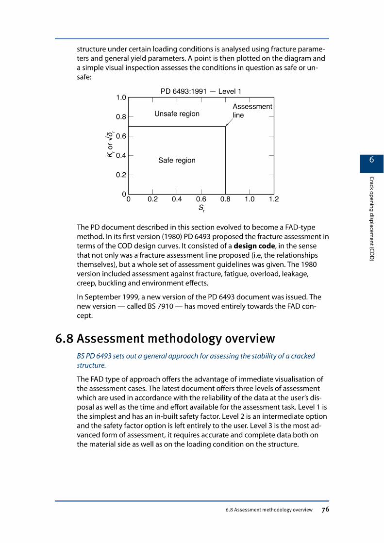
structure under certain loading conditions is analysed using fracture parame-ters and general yield parameters. A point is then plotted on the diagram anda simple visual inspection assesses the conditions in question as safe or un-safe:
The PD document described in this section evolved to become a FAD-typemethod. In its first version (1980) PD 6493 proposed the fracture assessment interms of the COD design curves. It consisted of a design code, in the sensethat not only was a fracture assessment line proposed (i.e, the relationshipsthemselves), but a whole set of assessment guidelines was given. The 1980version included assessment against fracture, fatigue, overload, leakage,creep, buckling and environment effects.
In September 1999, a new version of the PD 6493 document was issued. Thenew version — called BS 7910 — has moved entirely towards the FAD con-cept.
6.8 Assessment methodology overviewBS PD 6493 sets out a general approach for assessing the stability of a crackedstructure.
The FAD type of approach offers the advantage of immediate visualisation ofthe assessment cases. The latest document offers three levels of assessmentwhich are used in accordance with the reliability of the data at the user’s dis-posal as well as the time and effort available for the assessment task. Level 1 isthe simplest and has an in-built safety factor. Level 2 is an intermediate optionand the safety factor option is left entirely to the user. Level 3 is the most ad-vanced form of assessment, it requires accurate and complete data both onthe material side as well as on the loading condition on the structure.
6
Crack opening displacement (CO
D)
6.8 Assessment methodology overview 76
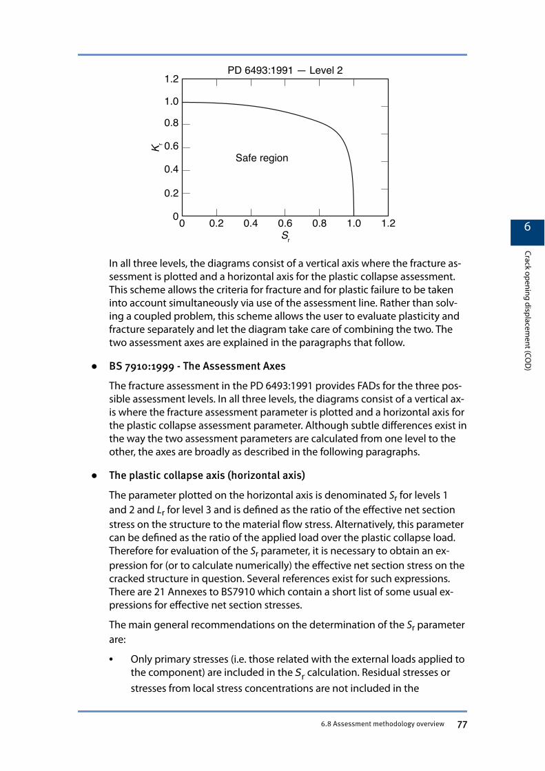
In all three levels, the diagrams consist of a vertical axis where the fracture as-sessment is plotted and a horizontal axis for the plastic collapse assessment.This scheme allows the criteria for fracture and for plastic failure to be takeninto account simultaneously via use of the assessment line. Rather than solv-ing a coupled problem, this scheme allows the user to evaluate plasticity andfracture separately and let the diagram take care of combining the two. Thetwo assessment axes are explained in the paragraphs that follow.
● BS 7910:1999 - The Assessment Axes
The fracture assessment in the PD 6493:1991 provides FADs for the three pos-sible assessment levels. In all three levels, the diagrams consist of a vertical ax-is where the fracture assessment parameter is plotted and a horizontal axis forthe plastic collapse assessment parameter. Although subtle differences exist inthe way the two assessment parameters are calculated from one level to theother, the axes are broadly as described in the following paragraphs.
● The plastic collapse axis (horizontal axis)
The parameter plotted on the horizontal axis is denominated Sr for levels 1and 2 and Lr for level 3 and is defined as the ratio of the effective net sectionstress on the structure to the material flow stress. Alternatively, this parametercan be defined as the ratio of the applied load over the plastic collapse load.Therefore for evaluation of the Sr parameter, it is necessary to obtain an ex-pression for (or to calculate numerically) the effective net section stress on thecracked structure in question. Several references exist for such expressions.There are 21 Annexes to BS7910 which contain a short list of some usual ex-pressions for effective net section stresses.
The main general recommendations on the determination of the Sr parameterare:
• Only primary stresses (i.e. those related with the external loads applied tothe component) are included in the Sr calculation. Residual stresses orstresses from local stress concentrations are not included in the
6
Crack opening displacement (CO
D)
6.8 Assessment methodology overview 77
calculation, since they cannot cause plastic collapse. Due to being de-nominated as primary stresses or loads, the symbol ‘p’ is sometimes usedto describe such stresses or loads.
Note
The terminology for stresses adopted in BS 7910:1999 is based on ASME VIII.
• Evaluation of Sr is usually based upon the value of the flow stress, definedarbitrarily as the average between the yield stress and the ultimate tensilestress (up to a limit of 1.2σy). This value is regarded as more meaningfulthan that of the yield stress, since it implies some allowance for workhardening.
The term ‘collapse load’ as adopted in the document does not correspond tothe strict definition of collapse for a structure as a whole, but more as a ratherlocalised event, where yield spreads through the wall thickness, e.g. for a part-through thickness flaw. For that reason, the term ‘effective net section stress’ ispreferred.
● The fracture axis (vertical axis)
For the fracture assessment, the applied stress system is again subdivided intoprimary stresses (those that can cause collapse) and secondary stresses (suchas residual stresses). The fracture assessment parameter is denominated Krand is defined as the ratio of the total applied stress intensity factor K over thematerial’s failure K. Primary and secondary stresses are treated in a slightly dif-ferent manner, basically due to the assumption that the plasticity associatedwith the primary stresses should be accounted for by the horizontal axis of theassessment diagram. In other words, plasticity from secondary stresses mightcause fracture, even though it might not cause collapse so it must be fully al-lowed for in the fracture assessment.
The applied stress intensity factor K is evaluated just as in LEFM, using the Yshape factors. Unknown residual stresses are assumed to be equal to the valueof the material’s yield stress.
The material KIc value is used if known. It may not be available because of thedifficulties in fracture testing for certain materials. In that case, a plasticitymeasure of toughness must be used — possibly a COD value or a KIcvalue ob-tained indirectly from a J-type test.
● The Assessment Levels
Level…
1. …is the simplest and has a large in-built safety factor.
2. …is an intermediate option where the safety factor is left entirely to theuser.
6
Crack opening displacement (CO
D)
6.8 Assessment methodology overview 78

3. …is the most advanced form of assessment, requiring accurate and com-plete data for both the material properties as well as the loadingconditions on the structure.
6
Crack opening displacement (CO
D)
6.8 Assessment methodology overview 79

80