Contents lists available at ScienceDirect

Mechanical Systems and Signal Processing

Mechanical Systems and Signal Processing 48 (2014) 260–273

http://d0888-32

n CorrE-m

journal homepage: www.elsevier.com/locate/ymssp

Parametric identification of a servo-hydraulic actuatorfor real-time hybrid simulation

Yili Qian a,n, Ge Ou b, Amin Maghareh b, Shirley J. Dyke a,b

a School of Mechanical Engineering, Purdue University, West Lafayette, IN 47907, USAb School of Civil Engineering, Purdue University, West Lafayette, IN 47907, USA

a r t i c l e i n f o

Article history:Received 29 May 2013Received in revised form3 February 2014Accepted 2 March 2014Available online 3 April 2014

Keywords:Servo-hydraulic actuatorsSystem identificationReal-time hybrid simulationGenetic algorithms

x.doi.org/10.1016/j.ymssp.2014.03.00170/& 2014 Elsevier Ltd. All rights reserved.

esponding author. Tel.: þ1 765 409 3430; faail address: ben.yiliqian@gmail.com (Y. Qian

a b s t r a c t

In a typical Real-time Hybrid Simulation (RTHS) setup, servo-hydraulic actuators serve asinterfaces between the computational and physical substructures. Time delay introduced byactuator dynamics and complex interaction between the actuators and the specimen hasdetrimental effects on the stability and accuracy of RTHS. Therefore, a good understanding ofservo-hydraulic actuator dynamics is a prerequisite for controller design and computationalsimulation of RTHS. This paper presents an easy-to-use parametric identification procedurefor RTHS users to obtain re-useable actuator parameters for a range of payloads. The criticalparameters in a linearized servo-hydraulic actuator model are optimally obtained fromgenetic algorithms (GA) based on experimental data collected from various specimen mass/stiffness combinations loaded to the target actuator. The actuator parameters demonstrateconvincing convergence trend in GA. A key feature of this parametric modeling procedure isits re-usability under different testing scenarios, including different specimen mechanicalproperties and actuator inner-loop control gains. The models match well with experimentalresults. The benefit of the proposed parametric identification procedure has been demon-strated by (1) designing an H1 controller with the identified system parameters thatsignificantly improves RTHS performance; and (2) establishing an analysis and computa-tional simulation of a servo-hydraulic system that help researchers interpret systeminstability and improve design of experiments.

& 2014 Elsevier Ltd. All rights reserved.

1. Introduction

Experimental testing is an essential tool for the global evaluation of civil structures, especially when new components arebeing considered to mitigate the destructive effects of natural disasters [1]. To conduct high efficiency and fidelity labtesting, Real-time Hybrid Simulation (RTHS) has been proposed. RTHS allows researchers to concentrate on the critical partsof a larger structure in a cost and time efficient way, while using numerical models to represent the other components andthus define the boundary conditions (Fig. 1) [1–3]. One of the major challenges to acquire reliable RTHS results is to achievesynchronization of boundary conditions between the computational and physical substructure [3].

The ability to reach synchronization of boundary conditions and perform reliable RTHS is often hindered by the time lagcaused by the dynamics of hydraulic actuators and control–structure interaction (CSI) [4]. Horiuchi [5] has shown that thelumped response delay is equivalent to negative damping in a real-time hybrid experiment which creates potential

x: þ1 765 494 0539.).

Fig. 1. RTHS System architecture.

Fig. 2. Block diagram of hydraulic actuator control structure in RTHS.

Y. Qian et al. / Mechanical Systems and Signal Processing 48 (2014) 260–273 261

instability in the system. Early efforts address this issue by approximating the time lag as a constant time delay andincluding compensation in the system [5]. Due to the fact that actuator dynamics (amplitude and phase) are rate dependentand the tracking bandwidth of RTHS (no more than 30 Hz) is usually higher than traditional structural testing methods [1],more complicated controller design methods have been proposed recently [3,6–8]. These controller design methods placean outer-loop controller (known as “controller” in the following text) outside the servo-hydraulic system loop formed by thehydraulic system controller (known as “inner-loop controller” in the following text), the actuator dynamics and the physicalspecimen (Fig. 2). Therefore, a reliable, practical and easy-to-use system identification method to model the entire servo-hydraulic loop is required.

Various servo-hydraulic system models have been considered in the literature. Although servo-hydraulic systems arenaturally nonlinear, experiments have shown that a linearized model is effective to represent the dynamics of the systemwithin its performance capacity [9,10]. Zhao [11] proposed a servo-hydraulic actuator system identification procedure foreffective force testing based on a white-box identification method. Because online measurement of each individualparameter in the hydraulic loop is generally infeasible, they were determined based on manufacturer specifications oreducated estimations. Alternatively, a black-box method was introduced by Jelali and Kroll [10] and is widely used for servo-hydraulic system control in structural testing [1,3,7,12]. However, since the system transfer function is established basedsolely on the measured input and output data sets, they do not have any physical significance and researchers have toconduct re-identification for another set of experimental setting. This process is especially cumbersome in many RTHSexperiments where researchers have to finely tune the inner-loop control gains or physical specimen characteristics (e.g.,magnetorheological damper (MR) control current/voltage). Another widely used identification method in structural testingis gray-box identification [8,13] which offers a compromise between white-box and black-box identification by establishinga parameterized model of the system but leaves specific parameter values to be obtained from an optimization technique[14,15].

However, parametric models presented in the literature are typically for a single experimental setup and the utilizationof these parameters is limited to establishing a transfer function in this specific case. It is thus worthwhile to establish anidentification procedure that could characterize the system's behavior in a range of payloads and inner-loop control gainswhich largely expands the advantages of the parametric model. This achievement would be especially helpful for servo-hydraulic systems in RTHS for the following reasons:

1.

Since the physical substructure in RTHS is usually nonlinear, a thorough understanding of the servo-hydraulic system'ssensitivity with respect to all payload parameters and inner-loop control gains is necessary in order to optimizecontroller design under a range of payload conditions [9]. This sensitivity analysis can be easily carried out with allactuator system parameters identified to decouple the dynamics of CSI and inner-loop feedback.

Y. Qian et al. / Mechanical Systems and Signal Processing 48 (2014) 260–273262

2.

A parametric model facilitates computational simulation of RTHS. The re-usability and independence of hydrauliccomponent parameters allow RTHS users to design optimal hardware and controller settings to prevent potentialinstability, which is common for RTHS, prior to an actual experiment. Computational simulation of RTHS is helpful todesign new RTHS experiments, including test setups where multiple actuators are involved [8].

3.

It enhances the understanding of servo-hydraulic system, including the contribution of each parameter to the overalldynamics. The parametric model and the computational simulation developed by the model could serve as a powerfulresult-interpretation tool [9] and reference [8] for RTHS, especially when instability is observed in the experiment.

4.

The robustness of the designed controller with respect to any realistic parameter identification error can be easily testedin a parametric model.

Herein, a general method is presented to identify the characteristic parameters of a servo-hydraulic actuator withina certain operation range to assist RTHS experiments. This approach will be applicable for modeling the same actuator withdifferent physical specimens and a case-by-case identification is no longer required. During the identification process,experimental data are collected with a series of known mass/spring components loaded to the actuator to analyze system'sbehavior under a range of payload conditions. Adequate knowledge of mechanical properties of these specimens enables usto extract actuator information from the coupled response of the actuator and the specimen. The system identificationproblem then evolves to a global optimization over the continuous parameter space corresponding to specimen variation.An objective function is selected to find the optimal value of each parameter and reflect the physical characteristics of thesystem. Genetic algorithms (GA) [16,17] are applied to efficiently perform the global search for the optimal values. Theproposed method is demonstrated to be effective for the purpose of controller design and computational simulation ofRTHS. It might be applied to other scenarios where the linearized system model is valid.

2. Problem formulation

2.1. Servo-hydraulic system modeling

A servo-hydraulic system is an arrangement of individual components connected to achieve hydraulic power transfer.The basic structure of a servo-hydraulic system consists of a hydraulic power supply, control elements (valves, sensors, etc.)and actuating elements (cylinders, etc.) [10]. Since the force/pressure output demand of a servo-hydraulic actuator for RTHSis typically negligible when compared with the power supply (i.e., pump) in the lab, only the dynamic responses of controland actuating elements will be considered here. The basic structure of the displacement-controlled system is shown inFig. 3. The displacement command generated within a computer through a real-time xPC target machine is transmitted tothe internal controller of the servo-hydraulic system which applies a proportional feedback control scheme to track theactuator performance by controlling the servo-valve to regulate hydraulic flow. The hydraulic flow enables the actuator tomove the target structure as well as sending out real-time displacement measurement from a linear variable differentialtransformer (LVDT) to complete the internal controller feedback loop.

The dashed line in Fig. 3 indicates the natural velocity feedback in the system. The coupling prevent researchers fromcompletely separating dynamic response of the structure and the actuator, and model them as independent components inseries [3]. A critical goal of this system identification study is to extract information related to the servo-hydraulic systemfrom the sampled data and derive its characteristic parameters independent of external loadings within a reasonable range.

The linearized model of each component in the servo-hydraulic system has been widely used in the literature[4,10,11,18–20] and adopted here. The modeling focuses on three stages of the system: servo-valve flow and its controller,actuator pressure dynamics, and test specimen dynamics.

Fig. 3. Block diagram of servo-hydraulic system.

Y. Qian et al. / Mechanical Systems and Signal Processing 48 (2014) 260–273 263

2.1.1. Servo-valve flow and its controllerPilot-stage valve dynamics

τ _QvpþQvp ¼ Kvpvi ð1ÞIn the Laplace domain

GvpðsÞ ¼QvpðsÞviðsÞ

¼ Kvp

τsþ1ð2Þ

where Kvp is the flow gain of the pilot-stage valve and τ is the equivalent time constant of the pilot-stage valve. Qvp is theflow through the pilot stage of the valve. vi is the valve control signal transmitted from the hydraulic system internalproportional controller: vi ¼ Kpxd. xd is the desired displacement sent from the controller.

It is assumed that spool position at main stage is proportional to the flow in the pilot stage, thus Main-stage valvedynamics

xv ¼ KcQvp ð3Þwhere Kc valve pressure gain that relates flow from the pilot stage to spool opening.

2.1.2. Actuator pressure dynamicsActuator pressure dynamics

QL ¼ Ka_PLþClPLþA_x ð4Þ

QL ¼ Kvxv

ffiffiffiffiffiffiffiffiffiffiffiffiffiffiffiffiffiffiffiffi1� xvPL

jxvjPs

sð5Þ

where Ka ¼ Vt=4βe, Vt is the volume of the actuator cylinder and βe is the effective bulk modulus of the fluid. Cl is theleakage coefficient of the piston from one chamber to another. A is the piston area. x is the displacement of the structure. A_xindicates the natural velocity feedback due to control–-structure interaction. PL and QL are the load pressure and flow rate,respectively. Kv is the flow gain of the servo-valve and Ps is the hydraulic supply pressure. When the load pressure isnegligible compared to the supply pressure the equation can be linearized as QL ¼ Kvxv.

2.1.3. Test specimen dynamicsThe load pressure and piston area yield the force applied to the test specimen. The response of the structure for a single-

degree-of-freedom specimen can be represented as

F ¼ PLA¼m€xþc_xþkx ð6Þand, in the Laplace domain, as

GacðsÞ ¼xðsÞPLðsÞ

¼ Ams2þcsþk

ð7Þ

wherem¼m0þmL and c¼ c0þcL;m0 is the mass of the actuator rod and all moving parts, c0 is the equivalent damping ratioof the actuator and mL and cL are the mass and damping of the test specimen, respectively. Since the actuator rod isconsidered to have an infinite stiffness, k is directly the stiffness of the test specimen.

2.1.4. Overall systemWith the dynamic equations for each servo-hydraulic system component, the overall system transfer function can be derived

with x as output displacement measurement and xd as input displacement command. The system can be represented in blockdiagram as shown in Fig. 4. Several important assumptions have been made in this mathematical model: (1) fluid properties

Fig. 4. Block diagram of the servo-hydraulic system in RTHS.

Table 1Servo-hydraulic system parameters in the transfer function.

Kv Valve flow gain Kc Valve pressure gainτ Servo-valve time delay constant c0 Actuator effective damping coefficientCl Piston leakage coefficient A Piston aream0 Actuator initial mass Vt Fluid volumeβe Effective bulk modulus Kvp Pilot stage valve flow gainmL Specimen mass k Specimen stiffnesscL Specimen damping Kp Inner-loop controller gain

Y. Qian et al. / Mechanical Systems and Signal Processing 48 (2014) 260–273264

(density, bulk modulus, etc.) are constant; (2) servo-valves are not saturated; (3) supply pressure is much greater than the loadpressure; (4) friction force can be modeled as viscous damping; and (5) main stage spool opening is proportional to pilot stage flow.These assumptions are acceptable in a typical RTHS setup where the servo-hydraulic system is operating within its nominal rangethat is usually constrained by: (1) the maximum capacity; and (2) the maximum allowable valve speed [10,11] specified by themanufacturer.

A number of parameters that need to be identified are listed in Table 1.Among all these parameters, the piston area is given by the manufacturer (here, 497 mm2), and the internal controller

proportional gain can be adjusted through the controller user interface. The specimen's mechanical properties (i.e. mL, k andcL) can be measured prior to the experiment. All remaining parameters are not available. To simplify the identificationprocess, some parameters are clustered together and defined as follows:

Z0 ¼ KvpKcKvA ð8Þ

Ka ¼ Vt=4βe ð9ÞBy defining these new parameters, the unknown parameters in the transfer function have been reduced to six. The

ultimate form of the system transfer function can be represented by a 4th order transfer function

Gxxd ðsÞ ¼XðsÞXdðsÞ

¼ Z0Kp

p1s4þp2s3þp3s2þp4sþp5ð10Þ

where

p1 ¼ Kaτm ð11Þ

p2 ¼ KaτcþτClmþKam ð12Þ

p3 ¼ KaτkþτClcþKacþA2τþmCl ð13Þ

p4 ¼ τClkþKakþA2þClc ð14Þ

p5 ¼ Z0KpþClk ð15Þ

2.1.5. LimitationsLinearized models similar to the one presented above have been proven experimentally to be quite effective overall in

capturing the salient dynamic characteristics of displacement-controlled, uni-axial and symmetric hydraulic actuators [9].For the majority of proof-of-concept RTHS experiments using actuators of similar size [1–3,18,19], the maximum frequencyof interest is less than 30 Hz and the amplitude is within 15 mm. The nonlinear behavior becomes especially significantwhen the actuator is operating beyond or near its maximum allowable operation range. One significant source ofnonlinearity comes from the valve flow. As the required spool opening increases, the flow gain Kv decreases and theassumption (5) in Section 2.1.4 is no longer valid. A detailed analysis of nonlinear behavior of the servo-valve can be found in[8] where more complicated system models are required.

2.1.6. Transfer function sensitivityTo help understand this linearized system model, we investigate the influence of specimen parameters on the system

transfer function. Specimen mass mL, stiffness k and internal controller gain Kp are the three variables for an experimentsetup [21]. Thus, they were each varied over a range to understand their influence on the transfer function.

Figs. 5–7 show the sensitivity of the system transfer function with specimen mass, stiffness and internal controller gainin numerical simulations. In each of the three cases the parameters (m, k and Kp) varied between 10% to 10 times of theoriginal value. By qualitative observation, internal controller gain variation has the most significant effect on the shape ofthe transfer function. Specimen mass and stiffness variation do not change the transfer function extensively especially interms of phase lag. However, it is worth noticing that innately, the system transfer function would not yield a unit gain due

Fig. 5. System transfer function sensitivity to specimen mass variation. Arrow indicates the increase in mass.

Fig. 6. System transfer function sensitivity to specimen stiffness variation. Arrow indicates the increase in stiffness.

Fig. 7. System transfer function sensitivity to controller gain variation. Arrow indicates increase in gain.

Y. Qian et al. / Mechanical Systems and Signal Processing 48 (2014) 260–273 265

to the Clk in the denominator when the stiffness is not zero. This phenomenon will not affect the functionality of the modelin most cases since Clk is usually relatively small compared to the numerator. When the specimen stiffness is large (e.g., astiff frame) the transfer function needs to be modified to satisfy the static condition. A general procedure to adjust the

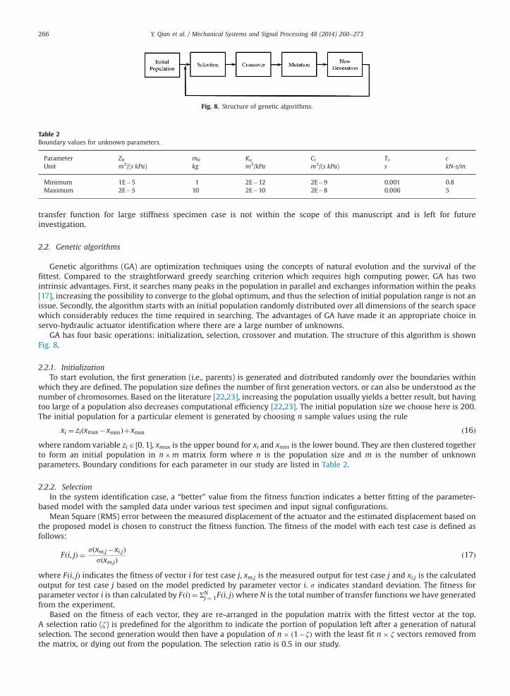
Fig. 8. Structure of genetic algorithms.

Table 2Boundary values for unknown parameters.

Parameter Z0 m0 Ka Cl Tv cUnit m3/(s kPa) kg m3/kPa m3/(s kPa) s kN-s/m

Minimum 1E�5 1 2E�12 2E�9 0.001 0.8Maximum 2E�5 10 2E�10 2E�8 0.006 5

Y. Qian et al. / Mechanical Systems and Signal Processing 48 (2014) 260–273266

transfer function for large stiffness specimen case is not within the scope of this manuscript and is left for futureinvestigation.

2.2. Genetic algorithms

Genetic algorithms (GA) are optimization techniques using the concepts of natural evolution and the survival of thefittest. Compared to the straightforward greedy searching criterion which requires high computing power, GA has twointrinsic advantages. First, it searches many peaks in the population in parallel and exchanges information within the peaks[17], increasing the possibility to converge to the global optimum, and thus the selection of initial population range is not anissue. Secondly, the algorithm starts with an initial population randomly distributed over all dimensions of the search spacewhich considerably reduces the time required in searching. The advantages of GA have made it an appropriate choice inservo-hydraulic actuator identification where there are a large number of unknowns.

GA has four basic operations: initialization, selection, crossover and mutation. The structure of this algorithm is shownFig. 8.

2.2.1. InitializationTo start evolution, the first generation (i.e., parents) is generated and distributed randomly over the boundaries within

which they are defined. The population size defines the number of first generation vectors, or can also be understood as thenumber of chromosomes. Based on the literature [22,23], increasing the population usually yields a better result, but havingtoo large of a population also decreases computational efficiency [22,23]. The initial population size we choose here is 200.The initial population for a particular element is generated by choosing n sample values using the rule

xi ¼ ziðxmax�xminÞþxmin ð16Þwhere random variable ziA ½0;1�, xmax is the upper bound for xi and xmin is the lower bound. They are then clustered togetherto form an initial population in n�m matrix form where n is the population size and m is the number of unknownparameters. Boundary conditions for each parameter in our study are listed in Table 2.

2.2.2. SelectionIn the system identification case, a “better” value from the fitness function indicates a better fitting of the parameter-

based model with the sampled data under various test specimen and input signal configurations.Mean Square (RMS) error between the measured displacement of the actuator and the estimated displacement based on

the proposed model is chosen to construct the fitness function. The fitness of the model with each test case is defined asfollows:

Fði; jÞ ¼ sðxm;j�xi;jÞsðxm;jÞ

ð17Þ

where Fði; jÞ indicates the fitness of vector i for test case j, xm;j is the measured output for test case j and xi;j is the calculatedoutput for test case j based on the model predicted by parameter vector i. s indicates standard deviation. The fitness forparameter vector i is than calculated by FðiÞ ¼ ΣN

j ¼ 1Fði; jÞwhere N is the total number of transfer functions we have generatedfrom the experiment.

Based on the fitness of each vector, they are re-arranged in the population matrix with the fittest vector at the top.A selection ratio (ζ) is predefined for the algorithm to indicate the portion of population left after a generation of naturalselection. The second generation would then have a population of n� ð1�ζÞ with the least fit n� ζ vectors removed fromthe matrix, or dying out from the population. The selection ratio is 0.5 in our study.

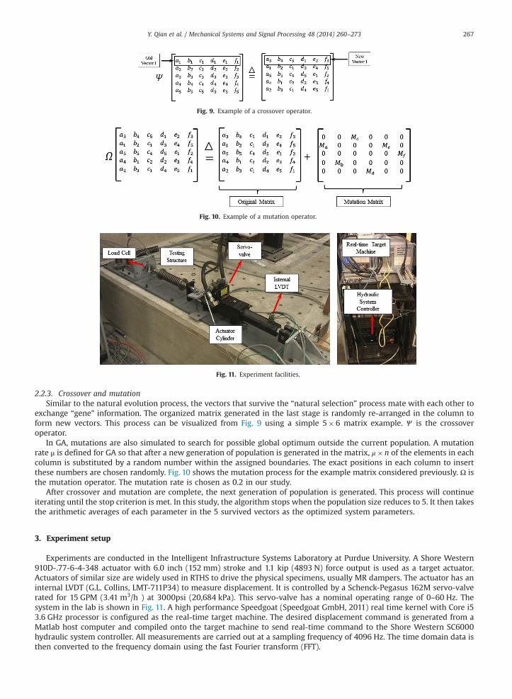
Fig. 9. Example of a crossover operator.

Fig. 10. Example of a mutation operator.

Fig. 11. Experiment facilities.

Y. Qian et al. / Mechanical Systems and Signal Processing 48 (2014) 260–273 267

2.2.3. Crossover and mutationSimilar to the natural evolution process, the vectors that survive the “natural selection” process mate with each other to

exchange “gene” information. The organized matrix generated in the last stage is randomly re-arranged in the column toform new vectors. This process can be visualized from Fig. 9 using a simple 5�6 matrix example. Ψ is the crossoveroperator.

In GA, mutations are also simulated to search for possible global optimum outside the current population. A mutationrate μ is defined for GA so that after a new generation of population is generated in the matrix, μ�n of the elements in eachcolumn is substituted by a random number within the assigned boundaries. The exact positions in each column to insertthese numbers are chosen randomly. Fig. 10 shows the mutation process for the example matrix considered previously. Ω isthe mutation operator. The mutation rate is chosen as 0.2 in our study.

After crossover and mutation are complete, the next generation of population is generated. This process will continueiterating until the stop criterion is met. In this study, the algorithm stops when the population size reduces to 5. It then takesthe arithmetic averages of each parameter in the 5 survived vectors as the optimized system parameters.

3. Experiment setup

Experiments are conducted in the Intelligent Infrastructure Systems Laboratory at Purdue University. A Shore Western910D-.77-6-4-348 actuator with 6.0 inch (152 mm) stroke and 1.1 kip (4893 N) force output is used as a target actuator.Actuators of similar size are widely used in RTHS to drive the physical specimens, usually MR dampers. The actuator has aninternal LVDT (G.L. Collins, LMT-711P34) to measure displacement. It is controlled by a Schenck-Pegasus 162M servo-valverated for 15 GPM (3.41 m3/h ) at 3000psi (20,684 kPa). This servo-valve has a nominal operating range of 0–60 Hz. Thesystem in the lab is shown in Fig. 11. A high performance Speedgoat (Speedgoat GmbH, 2011) real time kernel with Core i53.6 GHz processor is configured as the real-time target machine. The desired displacement command is generated from aMatlab host computer and compiled onto the target machine to send real-time command to the Shore Western SC6000hydraulic system controller. All measurements are carried out at a sampling frequency of 4096 Hz. The time domain data isthen converted to the frequency domain using the fast Fourier transform (FFT).

Fig. 12. Experimental setups for different specimens.

Table 3Test matrix.

No. Mass (kg) Stiffness (kN/m)

1 0 02 0.87 03 0.87 36.34 0.98 67.65 1.76 06 2.67 07 2.67 67.6

Y. Qian et al. / Mechanical Systems and Signal Processing 48 (2014) 260–273268

The physical specimens for system identification are a series of spring-mass sets tabulated in Table 3. These specimensare well-understood and can thus be helpful to separate the information of test specimen from the actuator system.A connector is attached to the actuator rod to make it compatible with various loading configurations. The structuralconfigurations shown in Fig. 12 are applied in our system identification procedure.

For each test specimen, three proportional gain and displacement amplitude values are used in an effort to derive a modelapplicable to a wider range of interest. The proportional gains and amplitudes chosen are Kp¼5,7,10; Amplitude¼0.02,0.05,0.1in (0.51, 1.27, 2.54 mm).

To fully excite system dynamics in all concerned frequency, we choose band-limited white noise (BLWN) with abandwidth of 0–80 Hz as our excitation for system identification.

4. Identification results

4.1. Data evolution

Fig. 13 shows the evolution of GA for two specific system characteristic values plotting over 12 generations: the Z0 valuedefined in Section 2 and the equivalent viscous damping in the actuator, c. As can be observed through the scatters, theinitially randomly scattered data within the boundaries converges to a smaller region of the parameter space as data gothrough the natural selection process. This trend can also be visualized by the evolution cost function value defined by Eq.(17) in Fig. 14. As population generation increases, this value decreases consistently, reaching a stably low value when thealgorithm meets its stop criterion.

4.2. Identification results

The identified parameters of the system transfer function are tabulated in Table 4.Based on the identified Ka value, and a rough estimation of the actuator cylinder volume using piston area and stroke, the

effective bulk modulus of the fluid is estimated as follows:

βe ¼14� Vchamber

Ka¼ 6� 10�4 m3

4� 1:39� 10�10 m3=kPa¼ 1:1� 106 kPa ð18Þ

where Vchamber is an estimation of the chamber volume based on bore diameter and chamber length. A reference value ofbulk modulus for hydraulic oil at the lab temperature is approximately 1.5�106 kPa [24,25] indicating a high fidelity in theidentified parameters.

2 4 6 8 10 12 14 16 18 206

8

10

12

14

16

18

20

22

24

Generation

Cos

t Fun

ctio

n V

alue

(inc

h)

Fig. 14. Fitness function value decreases as generation increases.

Table 4Identified system parameters.

Parameter Physical interpretation Value Unit

Z0 KvpKcKqA (Valve flow gains, pressure gain and piston area) 1.48E�05 m3/(s kPa)τv Valve time delay 0.0036 sCl Piston leakage coefficient 1E�8 m3/(s kPa)c Effective actuator damping 3.2 kN-s/mm0 Actuator initial mass 4.25 kgKa Vt/4βe (Chamber volume and fluid bulk modulus) 1.39E�10 m3/kPa

4 5 6 7 8 9 10

10

15

20

25

30

Actuator Viscous Damping (lb-s/in)

zg0

valu

e (in

3 -s/p

si)

Generation #1

4 5 6 7 8 9 10

10

15

20

25

30

Actuator Viscous Damping (lb-s/in)

Generation #4

4 5 6 7 8 9 10

10

15

20

25

30

Actuator Viscous Damping (lb-s/in)

Generation #8

4 5 6 7 8 9 10

10

15

20

25

30

Actuator Viscous Damping (lb-s/in)

Generation #12

zg0

valu

e (in

3 -s/p

si)

zg0

valu

e (in

3 -s/p

si)

zg0

valu

e (in

3 -s/p

si)

Fig. 13. Evolution of actuator damping c and Z0 value for GA generations 1,4,8 and 12.

Y. Qian et al. / Mechanical Systems and Signal Processing 48 (2014) 260–273 269

5 5.05 5.1 5.15 5.2 5.25 5.3 5.35 5.4 5.45 5.5-0.1

-0.05

0

0.05

0.1

0.15

Time (sec)

Dis

plac

emen

t (in

)

Desired DisplacementMeasured DisplacementModel Predicted Displacement

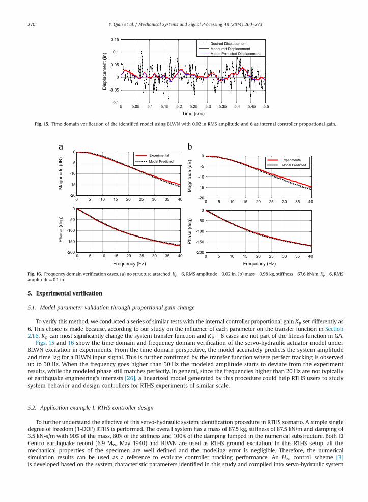
Fig. 15. Time domain verification of the identified model using BLWN with 0.02 in RMS amplitude and 6 as internal controller proportional gain.

0 5 10 15 20 25 30 35 40-20

-15

-10

-5

0

Mag

nitu

de (d

B) Experimental

Model Predicted

0 5 10 15 20 25 30 35 40-200

-150

-100

-50

0

Frequency (Hz)

Pha

se (d

eg)

0 5 10 15 20 25 30 35 40-20

-15

-10

-5

0

Mag

nitu

de (d

B) Experimental

Model Predicted

0 5 10 15 20 25 30 35 40-200

-150

-100

-50

0

Frequency (Hz)

Pha

se (d

eg)

Fig. 16. Frequency domain verification cases. (a) no structure attached, Kp¼6, RMS amplitude¼0.02 in. (b) mass¼0.98 kg, stiffness¼67.6 kN/m, Kp¼6, RMSamplitude¼0.1 in.

Y. Qian et al. / Mechanical Systems and Signal Processing 48 (2014) 260–273270

5. Experimental verification

5.1. Model parameter validation through proportional gain change

To verify this method, we conducted a series of similar tests with the internal controller proportional gain Kp set differently as6. This choice is made because, according to our study on the influence of each parameter on the transfer function in Section2.1.6, Kp can most significantly change the system transfer function and Kp ¼ 6 cases are not part of the fitness function in GA.

Figs. 15 and 16 show the time domain and frequency domain verification of the servo-hydraulic actuator model underBLWN excitation in experiments. From the time domain perspective, the model accurately predicts the system amplitudeand time lag for a BLWN input signal. This is further confirmed by the transfer function where perfect tracking is observedup to 30 Hz. When the frequency goes higher than 30 Hz the modeled amplitude starts to deviate from the experimentresults, while the modeled phase still matches perfectly. In general, since the frequencies higher than 20 Hz are not typicallyof earthquake engineering's interests [26], a linearized model generated by this procedure could help RTHS users to studysystem behavior and design controllers for RTHS experiments of similar scale.

5.2. Application example I: RTHS controller design

To further understand the effective of this servo-hydraulic system identification procedure in RTHS scenario. A simple singledegree of freedom (1-DOF) RTHS is performed. The overall system has a mass of 87.5 kg, stiffness of 87.5 kN/m and damping of3.5 kN-s/m with 90% of the mass, 80% of the stiffness and 100% of the damping lumped in the numerical substructure. Both ElCentro earthquake record (6.9 Mw, May 1940) and BLWN are used as RTHS ground excitation. In this RTHS setup, all themechanical properties of the specimen are well defined and the modeling error is negligible. Therefore, the numericalsimulation results can be used as a reference to evaluate controller tracking performance. An H1 control scheme [3]is developed based on the system characteristic parameters identified in this study and compiled into servo-hydraulic system

Y. Qian et al. / Mechanical Systems and Signal Processing 48 (2014) 260–273 271

controller. The target loop shape of the H1 controller is set as follows:

GdðsÞ ¼1:2� 106

0:008s3þ20s2þ65sþ1200ð19Þ

Using the identified parameters in Section 4.2, the transfer function of the actuator system is

GðsÞ ¼ 12:44

2:129� 10�8s4þ1:181� 10�5s3þ0:703sþ13:98ð20Þ

Eqs. (19) and (20) are used in Matlab to design a H1 controller for the system. Details of this controller design methodcan be found in [3].

Figs. 17 and 18 show the time domain and frequency domain performance of RTHS using model based controller,respectively. With the application of a model based controller, the time lag associated with actuator dynamics, which can beobserved clearly in the un-controlled RTHS case, has largely been removed. The RTHS result is very close to the numericalsimulation result which has high fidelity based on our simple structure selection. The remaining errors and time lags, asmentioned at the beginning, are due to modeling and measurement errors, computation time steps, and integration scheme.The trend becomes more apparent when the data are transferred to the frequency domain in Fig. 18. This model basedcontroller has successfully preserved the amplitude and phase characteristics of the input signal within 30 Hz. The identifiedcharacteristic parameters of this system are used to simulate the dynamic performance of the system in order to tune thebest controller parameters before it is applied to the experiment facilities.

1 2 3 4 5 6 7 8 9 10-0.4

-0.2

0

0.2

0.4

Time (sec)

Dis

plac

emen

t (in

) RTHS with Model-Based ControllerRTHS without Model-Based ControllerNumerical Simulation

4 4.1 4.2 4.3 4.4 4.5 4.6 4.7 4.8 4.9 5-0.4-0.3-0.2-0.1

00.10.20.3

Time (sec)

Dis

plac

emen

t (in

)

Fig. 17. Time domain comparison between RTHS with model-based H1 controller, RTHS without model-based controller and numerical simulation result.The SDOF target structure is simple enough that its numerical simulation response can be considered as an accurate representation of its actual behaviorand can thus be used as a reference.

0 5 10 15 20 25 30-15

-10

-5

0

5

10

Frequency (Hz)

Mag

nitu

de (d

B)

0 5 10 15 20 25 30-120-100-80-60-40-20

020

Frequency (Hz)

Ang

le (D

eg)

RTHS with Model-Based ControllerRTHS without Model-Based Controller

Fig. 18. Frequency domain comparison between RTHS with model-based H1 controller and RTHS without model-based controller.

0 10 20 30 40 500.5

0.6

0.7

0.8

0.9

1

Mag

nitu

de (d

B)

ExperimentalModel Predicted

0 10 20 30 40 50-250

-200

-150

-100

-50

0

Frequency (Hz)

Pha

se (d

eg)

0 10 20 30 40 500.5

1

1.5

2

Mag

nitu

de (d

B)

ExperimentalModel Predicted

0 10 20 30 40 50-250

-200

-150

-100

-50

0

Frequency (Hz)

Pha

se (d

eg)

Fig. 19. Comparison between transfer functions obtained from experimental data and parametric model. (a) Inner-loop gain 2, amplitude 0.08 in; (b) inner-loop gain 3, amplitude 0.04 in.

Y. Qian et al. / Mechanical Systems and Signal Processing 48 (2014) 260–273272

5.3. Application example II: instability interpretation from oil-column resonance

A parametric model of the servo-hydraulic system facilitates the understanding of the contribution of each systemparameter to the overall dynamics and helps establish computational simulation of RTHS. Therefore, it serves as a powerfultool to interpret, predict and remove the unwanted effects in the system.

Here we reinforce the benefits of parametric modeling in a different hardware setup for simple displacement trackingwithout outer-loop controller. We use a Shore Western 910D-.37-4-4-1348 actuator using similar elements and configura-tion as the one we identified in Section 3, the major difference being the actuator piston area changing from 0.77 in2

(496 mm2) to 0.37 in2 (239 mm2) and the stroke changing from 6.0 in (162.4 mm) to 4.0 in (101.6 mm). The test specimen isa one story building model that has an equivalent mass of 2.06 kg and equivalent stiffness of 30.65 kN/m. Undesiredsustained oscillation is observed in the experiments at around 45 Hz (Fig. 19). This oscillation can be easily interpreted withthe parametric model presented in this paper as explained below.

The parametric transfer function (10) shows that actuator volume, the major change in this setup, always appearstogether with the bulk modulus as defined by Ka. Because bulk modulus characterizes the compressibility of the hydraulicfluid, one can easily associate this parameter with the resonance of the hydraulic fluid in the actuator chamber, known asoil-column resonance [8,11]. In fact, it is a common source of instability in RTHS. Zhao [11] has shown that slightly dampedoil-column resonance can easily drive the system unstable on the root-locus plane. Therefore, predicting and decreasing theimpact of oil-column resonance are an important design consideration in RTHS.

In this case study, by changing the parameter values for piston area and chamber volume in the model we deducedpreviously, we can easily obtain a computational simulation for this new servo-hydraulic system setup without conductingsystem identification experiments. Although we use the model here to interpret existing experimental results, the samesimulation can be easily done prior to actual experiment to help researchers predict system behavior and avoid potentialinstability. Furthermore, simulations can shed some light on improving system design. As shown in Fig. 19, reducing inner-loop control gain reduces the effect of oil-column resonance in this case.

6. Conclusion

This paper presents a high fidelity and efficient general procedure to derive a parametric model for servo-hydraulicactuators involved in RTHS. The system transfer function is derived from a fourth-order, component-based linearized modelof the servo-hydraulic system. Known parameters from the design of the actuator and the physical test setup are employedin the model. The remaining parameters in the experimental transfer function are identified using a series of white noiseinputs with varying payloads. Genetic algorithms are used to optimize system characteristic parameters in this transferfunction. Various test specimens are attached to the actuator, and the dynamics in each case is compared with themathematical model to generate a fitness function in GA.

The proposed approach is found to be highly efficient and has fast convergence for this application and the results of theparametric identification are demonstrated to be effective. The resulting model is evaluated using different specimen casesand yields a good match between experimental results and predicted responses. A parametric model helps RTHS users to

Y. Qian et al. / Mechanical Systems and Signal Processing 48 (2014) 260–273 273

better understand the dynamics of the system (especially its sensitivity to each parameter) and establish computationalsimulation of RTHS that helps to select the best experiment setup. The application of the method is demonstrated throughtwo examples: (1) the design and implementation of an H-infinity controller for RTHS, which yielded improved actuatordisplacement control performance in RTHS; (2) a brief system analysis that interprets the oil-column resonance which canbe expanded to predict system behavior and improve experiment design.

Acknowledgment

This project is supported by National Science Foundation Grant number NSF-1136075 and Purdue University SummerUndergraduate Research Fellowship (SURF) program.

References

[1] J.E. Carrion, B.F. Spencer, Model-based Strategies for Real-time Hybrid Testing, The Newmark Structural Engineering Laboratory, Urbana, 2007.[2] X. Shao, A.M. Reinhorn, M.V. Sivaselvan, Real-time hybrid simulation using shake tables and dynamic actuators, J. Struct. Eng. 137 (7) (2011) 748–760,

http://dx.doi.org/10.1061/(ASCE)ST.1943-541X.0000314.[3] X. Gao, N. Castaneda, S.J. Dyke, Real time hybrid simulation: from dynamic system, motion control to experimental error, Earthq. Eng. Struct. Dyn. 42

(6) (2013) 815–832, http://dx.doi.org/10.1002/eqe.2246.[4] S.J. Dyke, B.F. Spencer, P. Quast, M. Sain, Role of control-structure interaction in protective system design, ASCE J. Eng. 121 (2) (1995) 332–338, http:

//dx.doi.org/10.1061/(ASCE)0733-9399(1995)121:2(322).[5] T. Horiuchi, M. Inoue, T. Konno, Y. Namita, Real-time hybrid experimental system with actuator delay compensation and its application to a piping

system with energy absorber, Earthq. Eng. Struct. Dyn. 28 (10) (1999) 1121–1141.[6] C. Chen, J.M. Rickles, Tracking error-based servo-hydraulic actutor adaptive compensation for real-time hybrid simulation, J. Struct. Eng. 136 (4) (2010)

432–440, http://dx.doi.org/10.1061/ASCEST.1943-541X.0000124.[7] B.M. Phillips, B.F. Spencer, Model-based feddforward-feedback actuator control for real-time hybrid simulation, J. Struct. Eng. 139 (2012) 1205–1214,

http://dx.doi.org/10.1061/(ASCE)ST.1943-541X.0000606.[8] N. Nakata, E. Krug, Computational framework for effective force testing and a compensation technique for nonlinear actuator dynamics, Struct. Control

Health Monitor. (2013), http://dx.doi.org/10.1002/stc.1599.[9] J.P. Conte, T.L. Trombetti, Linear dynamic modeling of a uni-acial servo-hydraulic shaking table system, Earthq. Eng. Struct. Dyn. 29 (9) (2000)

1375–1404.[10] M. Jelali, A. Kroll, Hydraulic Servo-System Modeling, Identification and Control, Springer-Verlag, London, 2003.[11] Zhao, J. (2003). Develop of EFT for nonlinear SDOF system (Ph.D. thesis), University of Minnesota.[12] C.N. Lim, S.A. Neild, D.P. Stoten, D. Drury, C.A. Taylor, Adaptive control strategy for dynamic substructuring tests, J. Eng. Mech. 133 (8) (2007) 864–873.[13] T. Tidwell, X. Gao, H.-M. Huang, S.J. Dyke, C. Gill, (2009). Towards configurable real-time hybrid structural testing: a cyber-physical systems approach,

in: Proceeding of IEEE International Symposium on Object, Component, Service-oriented Real-Time Distributed Computing, Tokyo,pp. 37–44, http://dx.doi.org/10.1109/ISORC.2009.41.

[14] H. Garnier, L. Wang, Identification of Continuous-time Models from Sampled Data, Springer-Verlag, London, 2008.[15] B. Boulet, L. Daneshmend, V. Hayward, C. Nemri (1991). System identification and modelling of a high performance hydraulic actuator,in: The Second

International Symposium on Experimental Robotics, Toulouse, France, pp. 505-520.[16] J.H. Holland, Adaption in Natural and Aritificial Systems, University of Michigan Press, Ann Arbor, 1975.[17] K. Kristinsson, G. Dumont, System identification and control using genetic algorithms, IEEE Trans. Syst. Man Cybern. 22 (5) (1992) 1033–1046.[18] B.M. Phillips, B.F. Spencer, Model-Based Servo-Hydraulic Control for Real-Time Hybrid Simulation, University of Illinois at Urbana-Champaign, Urbana-

Champaign, 2011.[19] N. Nakata, Effective force testing using a robust loop shaping controller, Earthq. Eng. Struct. Dyn. 42 (2) (2012) 261–275, http://dx.doi.org/10.1002/

eqe.2207.[20] C. De Silva, Control Sensors and Actuators, Prentice Hall, Englewood Cliffs, NJ, 1989.[21] Gao, X. (2012). Development of a robust framework for real-time hybrid simulation: from dynamical system, motion control to experimental error

verification (Ph.D. thesis), Purdue University.[22] H. Yousefi, H. Handroos, A. Soleymani, Application of differential evolution in system identification of a servo-hydraulic system with a flexible load,

Mechatronics 18 (9) (2008) 513–528, http://dx.doi.org/10.1016/j.mechatronics.2008.03.005.[23] Sarmady, S. (2007). An Investigation on Genetic Algorithm Parameters. School of Computer Science, Universiti Sains Malaysia.[24] S. Kim, H. Murrenhoff, Measurement of effective bulk modulus for hydraulic oil at low pressure, J. Fluid Eng. 134 (2) (2012), http://dx.doi.org/10.1115/

1.4005672.[25] P.J. Pritchard, J.C. Leylegian, Fox and McDonald's Introduction to Fluid Mechanics, John Wiley and Sons, INC, 2011.[26] E.M. Rathje, N.A. Abrahamson, J.D. Bray, Simplified frequency content estimates of earthquake ground motions, J. Geotech. Geoenviron. Eng. 124 (2)

(1998) 150–159, http://dx.doi.org/10.1061/(ASCE)1090-0241(1998)124:2(150).