MECHANICAL PROPERTIES OF INTERLAYERS IN · PDF fileMaster’s Dissertation Structural...

Master’s DissertationStructuralMechanics

CAMILLA FORS

MECHANICAL PROPERTIES OFINTERLAYERS IN LAMINATED GLASSExperimental and Numerical Evaluation

DEPARTMENT OF CONSTRUCTION SCIENCES

DIVISION OF STRUCTURAL MECHANICS

ISRN LUTVDG/TVSM--14/5198--SE (1-52) | ISSN 0281-6679

MASTER’S DISSERTATION

Supervisor: KENT PERSSON, PhD, Div. of Structural Mechanics, LTH, Lund

Examiner: Professor PER JOHAN GUSTAFSSON, Div. of Structural Mechanics, LTH, Lund.

Copyright © 2014 Division of Structural MechanicsFaculty of Engineering (LTH), Lund University, Sweden.

Printed by Media-Tryck LU, Lund, Sweden, October 2014 (Pl).

For information, address:Div. of Structural Mechanics, LTH, Lund University, Box 118, SE-221 00 Lund, Sweden.

Homepage: http://www.byggmek.lth.se

CAMILLA FORS

MECHANICAL PROPERTIES OFINTERLAYERS IN LAMINATED GLASS

Experimental and Numerical Evaluation

AbstractThe architectural and engineering trend leads towards greater use of glass in buildings.Growing safety awareness often requires laminated glass. Laminated glass is formedas a sandwich of two or more sheets of glass and a plastic interlayer. Laminated glasscan for example be used in stairs, floors, roofs, facades and balcony railings.

This thesis deals with the most common interlayer polyvinyl butyral (PVB). Thereare many varieties of PVB and this thesis investigates the mechanical properties ofa variety of PVB. Experimental tensile tests have been conducted on six PVB withvarious properties. The tests have been conducted with different loading rates to takethe time dependency into account. PVB shows time and temperature dependencyand in numerical simulations it is often simplified as a linear elastic material. Byusing the generalized Maxwell model, which is a mechanical model that describes alinear viscoelastic material behaviour, a Prony series have been determined from theexperimental tests. A tensile test has been modelled in the commercial finite elementsoftware Abaqus. The Prony series have been implemented in the Abaqus-modelto create a viscoelastic material model. The model has been created for of one ofthe experimentally tested interlayers, a standard PVB with a thickness of 0.76 mm.Thereafter the viscoelastic model has been used in a laminated glass model to showhow the time of loading affects the structural behaviour.

The results from the experimental tests show that there are differences in all thetested PVB. Some are stiffer, and some are softer. The numerical tensile test modelwas in good agreement with the laboratory results for standard PVB 0.76 mm. Thenumerical application where a laminated glass unit was subjected to long-term andshort-term loads showed a loss in structural resistance due to the time dependentbehaviour. One could see that with longer loading time, an increase in the stressesoccur and the plate behaves more like a layered unit than a monolithic plate. Thisleads to the conclusion that it is important to take into account the time dependentbehaviour when using laminated glass as a structural element.

Keywords: Laminated glass, Interlayers, PVB, Viscoelasticity, Prony series, Gener-alized Maxwell model, FEM, Abaqus, Tensile test

i

SammanfattningTrender inom arkitektur och ett större intresse hos ingenjörer för glas har lett tillett ökat användande av glas i byggnader. Ökat säkerhetsmedvetande kräver ofta attlaminerat glas används. Laminerat glas består av två eller flera lager av glas medmellanskikt av plastfolie. Laminerat glas kan användas i exempelvis trappor, golv,tak, fasader och balkongräcken.

Detta examensarbete studerar den mest vanliga plastfolien polyvinyl butyral (PVB).Det finns många olika typer av PVB och syftet är att undersöka de mekaniska egen-skaperna hos olika PVB. Experimentella dragprov har gjorts på sex PVB med olikaegenskaper. Testerna har gjorts med olika töjningshastigheter för att ta hänsyn tilltidsberoendet hos folien. PVB uppvisar ett tids- och temperaturberoende och fören-klas ofta som ett linjärt elastiskt material i numeriska simulationer. Genom att an-vända sig av den generaliserade Maxwell modellen, som är en mekanisk modell sombeskriver ett linjärt viskoelastiskt beteende, har en Prony-serie bestämts utifrån deexperimentella resultaten. Ett dragprov har modellerats i finita element program-met Abaqus. Prony-serien har implementerats i Abaqus-modellen för att skapa enviskoelastisk materialmodell. Modellen har skapats för ett av de testade mellanskik-ten, standard PVB med tjockleken 0,76 mm. Därefter har en skiva av laminerat glasmodellerats i Abaqus där den viskoelastiska materialmodellen har använts. DennaAbaqus-modell har gjorts för att visa hur lastvaraktigheten påverkar konstruktionensbärförmåga.

Resultaten från dragproven visade att de mekaniska egenskaperna skiljde sig blandde provade plastfolierna. Några av dem var styvare, medan andra var mjukare. Drag-provsmodellen i Abaqus med viskoelastisk materialmodell stämde bra överens med delaborativa värdena för standard PVB 0,76 mm. I den numeriska tillämpningen där enlaminerad glasskiva var belastad med korttids- och långtidslaster uppvisades en förlusti lastförmåga på grund av det tidsberoende beteendet hos folien. Resultatet visade attspänningarna ökade med en längre lastvaraktighet. Det laminerade glaset betedde sigmer som om plastfolien inte fanns, som två glasskivor, än som en monolitisk skiva vidlång lastvaraktighet. Detta leder till slutsatsen att det är viktigt att ta hänsyn till dettidsberoende beteendet när laminerat glas används som bärande element.

Nyckelord: Laminaterat glas, mellanskikt, PVB, viskoelasticitet, Prony-serie, gener-aliserad Maxwell modell, FEM, Abaqus, dragprov

iii

PrefaceFive years have passed since I started my studies at LTH. When I started my studiessomeone told me that you could use glass to build columns. At that time I could notbelieve it was true but I found it very interesting. I have always had an interest inarchitecture and started to think about how glass columns can change the aestheticlook of a building, but I got even more curious about how such a brittle material couldbe used as a structural element.

My studies went on and in my fourth year I went to Germany to study one semesterat Technische Universität München. In Munich I got the opportunity to learn moreabout glass in the course Structural Design of Glass Constructions taught by ProfessorMartin Mensinger. With interesting lectures and an inspiring excursion I got moreinterested in laminated glass. Then a thought started to grow, I wanted to write mymaster thesis about glass.

I am very thankful for having Kent Persson as my supervisor. He always had hisdoor open and helped me with all my questions. So my acknowledgement goes directlytowards Kent Persson at the Structural Mechanics Department for all his help duringthis thesis. I would like to thank Forserum Safety Glass for making it possible to doexperimental tests by delivering interlayers to evaluate. I am also thankful to ZivoradZivkovic at the Solid Mechanics Department for helping me out with the experimentaltests.

Now, my five years have come to an end. Thanks Lund University for all theopportunities you have given me and thanks to all my friends for making these fiveyears such an unforgettable time!

Lund, August 2014

v

Contents

1 Introduction 11.1 Background . . . . . . . . . . . . . . . . . . . . . . . . . . . . . . . . . 11.2 Objective and Method . . . . . . . . . . . . . . . . . . . . . . . . . . . 21.3 Scope and Delimitation . . . . . . . . . . . . . . . . . . . . . . . . . . . 21.4 Thesis Outline . . . . . . . . . . . . . . . . . . . . . . . . . . . . . . . . 2

2 Laminated Glass 32.1 Glass . . . . . . . . . . . . . . . . . . . . . . . . . . . . . . . . . . . . . 3

2.1.1 Manufacturing of Float Glass . . . . . . . . . . . . . . . . . . . 32.1.2 Mechanical Properties . . . . . . . . . . . . . . . . . . . . . . . 42.1.3 Heat-treated Glass . . . . . . . . . . . . . . . . . . . . . . . . . 5

2.2 Laminated Glass . . . . . . . . . . . . . . . . . . . . . . . . . . . . . . 72.2.1 Interlayers . . . . . . . . . . . . . . . . . . . . . . . . . . . . . . 72.2.2 Structural Behaviour of Laminated Glass . . . . . . . . . . . . . 82.2.3 Post-breakage Behaviour . . . . . . . . . . . . . . . . . . . . . . 9

2.3 Current Standards, Guidelines and Design Methods . . . . . . . . . . . 10

3 Experimental Tests 113.1 Performed Tests . . . . . . . . . . . . . . . . . . . . . . . . . . . . . . . 113.2 Test Design . . . . . . . . . . . . . . . . . . . . . . . . . . . . . . . . . 113.3 Stress-strain Diagram . . . . . . . . . . . . . . . . . . . . . . . . . . . . 133.4 Results . . . . . . . . . . . . . . . . . . . . . . . . . . . . . . . . . . . . 143.5 Discussion . . . . . . . . . . . . . . . . . . . . . . . . . . . . . . . . . . 14

4 Material Model 174.1 Mechanical Model . . . . . . . . . . . . . . . . . . . . . . . . . . . . . . 17

4.1.1 Mechanical Models for Viscoelasticity . . . . . . . . . . . . . . . 174.1.2 Application to Standard PVB 0.76 mm . . . . . . . . . . . . . . 19

5 Finite Element Study 235.1 The Finite Element Method . . . . . . . . . . . . . . . . . . . . . . . . 23

5.1.1 Elements in Abaqus . . . . . . . . . . . . . . . . . . . . . . . . 235.2 Finite Element Model . . . . . . . . . . . . . . . . . . . . . . . . . . . . 24

5.2.1 Material Model . . . . . . . . . . . . . . . . . . . . . . . . . . . 255.2.2 Boundary Conditions . . . . . . . . . . . . . . . . . . . . . . . . 255.2.3 Element Type and Mesh . . . . . . . . . . . . . . . . . . . . . . 26

vii

5.2.4 Analysis and Step . . . . . . . . . . . . . . . . . . . . . . . . . . 265.3 Results . . . . . . . . . . . . . . . . . . . . . . . . . . . . . . . . . . . . 265.4 Discussion . . . . . . . . . . . . . . . . . . . . . . . . . . . . . . . . . . 27

6 Numerical Application of the Viscoelastic Model 296.1 FE Model . . . . . . . . . . . . . . . . . . . . . . . . . . . . . . . . . . 296.2 Result . . . . . . . . . . . . . . . . . . . . . . . . . . . . . . . . . . . . 306.3 Discussion . . . . . . . . . . . . . . . . . . . . . . . . . . . . . . . . . . 31

7 Results 33

8 Conclusions and Future Work 358.1 Conclusions . . . . . . . . . . . . . . . . . . . . . . . . . . . . . . . . . 358.2 Future Work . . . . . . . . . . . . . . . . . . . . . . . . . . . . . . . . . 35

A Experimental Test Results 39A.1 Load Rate 200 mm/min . . . . . . . . . . . . . . . . . . . . . . . . . . 39A.2 Load Rate 50 mm/min . . . . . . . . . . . . . . . . . . . . . . . . . . . 42A.3 Load Rate 10 mm/min . . . . . . . . . . . . . . . . . . . . . . . . . . . 45A.4 Load Rate 2 mm/min and 0.5 mm/min . . . . . . . . . . . . . . . . . . 49

B Loads 51B.1 Snow Load . . . . . . . . . . . . . . . . . . . . . . . . . . . . . . . . . . 51B.2 Wind Load . . . . . . . . . . . . . . . . . . . . . . . . . . . . . . . . . 51

viii

Chapter 1

Introduction

1.1 BackgroundThe architectural and engineering trend leads towards greater use of glass in buildings.Growing safety awareness often requires laminated glass. Laminated glass is formedas a sandwich of two or more sheets of glass and a plastic interlayer, see Figure 1.1.Laminated glass can for example be used in stairs, floors, roofs, facades and balconyrailings. The interlayer is typically soft polymers like polyvinyl butyral (PVB), ethylvinyl acetate (EVA) and SentryGlas® (SGP) from the company DuPont. When lam-inated glass shatters, the plastic interlayer keeps the pieces of glass in place. Thisreduces the risk of cuts caused by splinters.

Today there are many interlayers on the market with a large variation in theirproperties. For every project, in different areas of use, it is a challenging task tochoose the most optimal interlayer.

PVB is the most common interlayer used in laminated glass and over the yearsmany new varieties of PVB have been developed. Previous works on the mechanicalproperties of the interlayer have mainly focused on standard PVB. More recent researchhas been done on SGP and the results have been compared to PVB. At this time, noneor little research have been done comparing a variety of PVB.

Glass is a complex material, and so is the behaviour of the viscoelastic materialPVB. Therefore laminated glass is often analysed in a finite element program to capturethe complex behaviour. PVB is often simplified as linear elastic material, this ishowever not the case due to the temperature and time dependent behaviour.

GlassInterlayer

Glass

Figure 1.1: Laminated glass

1

1.2 Objective and MethodThe main objective of this master thesis is to investigate a variety of interlayers ofthe type PVB and their mechanical properties. To evaluate the interlayers tensiletests with different strain rates will be conducted. A method on how to create aviscoelastic model from laboratory test suitable for implementations in a finite elementprogram will be presented. For one of the tested interlayers, standard PVB 0.76 mm, aviscoelastic model suitable for simulations will be proposed as well as the procedure toderive it. A finite element model with a laminated glass unit subjected to short-termand long-term loads will be presented. This model will show how the time of loadingaffects the structural behaviour.

The finite element analyses will be done with the software Abaqus. The experi-mental tests and the numerical analyses will lead to guidelines on suitable interlayersfor different field of applications.

1.3 Scope and DelimitationThe scope of the thesis is to evaluate the time dependent behaviour of the interlayer;however the temperature-dependency will be excluded.

1.4 Thesis OutlineThe thesis is divided into several sections:

• Section 2 gives an introduction to the material glass and more detailed informa-tion about laminated glass.

• Section 3 explains the experimental tests. The results and discussion are alsopresented here.

• Section 4 describes mechanical models and the model used in the finite elementanalysis.

• Section 5 explains the finite element study. Here are also the results and discus-sion presented.

• Section 6 presents a finite element model with a laminated glass unit subjectedto snow and wind load.

• Section 7 presents a summary of the results from the experimental tests and thefinite element study.

• Section 8 discusses and draws conclusions from the results presented in section7. Suggestions to possible further work are presented here.

2

Chapter 2

Laminated Glass

The mechanical properties of the interlayer are of high importance when using lami-nated glass as a structural element. To understand the structural behaviour of lami-nated glass it is also important with knowledge about glass.

In this chapter information of the material glass and laminated glass is provided.The first section treats the basics of glass, the manufacturing of float glass, the mechan-ical properties and post processing of float glass (heat-treated glass). In the secondsection laminated glass is described with information about the structural behaviour,the post-breakage behaviour, the properties of the interlayer and the current standards,guidelines and design methods for laminated glass.

2.1 GlassGlass is a solid material that is hard and brittle. It is an amorphous solid, also calleda non-crystalline solid, which means that the atomic structure is disordered [8]. Glassdoes not have an exact melting point like other materials; instead it transforms froma liquid to a solid state over a certain temperature range, usually around 500°C. Oneimportant property of glass is its high resistance to many chemicals which makes it avery durable material [8].

There are numerous types of glass with varying chemical and physical propertiesdepending on the area of use. The most common glass is the soda-lime glass, also calledsoda-lime-silica glass. Soda-lime glass contains the raw materials sand (contains silica),soda ash and limestone, and also a smaller amount of various additives [8].

2.1.1 Manufacturing of Float GlassFlat glass is the most commonly used glass in laminated glass and is typically madeof soda-lime glass. Flat glass can be produced in different ways; however the so calledfloat glass procedure stands for 90% of the production of flat soda-lime glass [11]. Inthe float process, invented by Pilkington in year 1959, the glass is produced by lettingmolten glass float on a bath of liquid tin, see Figure 2.1. By this procedure the glassgets a flat surface on both sides [8]. The thickness of the float glass is controlled bythe speed of which the glass is drawn off from the tin bath [15]. The glass is then

3

Figure 2.1: The float process [13]

Chemical composition

Manufacturingprocess

Finishing

Glass

Soda-lime glass

Float glass (annealed glass, monolithic glass)

Heat treated glass

Laminated glass

Heat strengthened glass Fully tempered glass

Figure 2.2: Overview of the most important glass products and the steps of processing

cooled down slowly after the tin bath in the annealing lehr, which is a long tunneloven [13, 11]. The annealing process removes the internal stresses in the material bythe controlled cooling process. It is of high importance with a controlled, slow coolingsince uneven cooling can lead to a reduction of the mechanical strength. Anotherterm for float glass is annealed glass. The last steps in the float process is inspectionand cutting of the glass before delivering it to the customer [13]. However, the floatglass can be processed further to produce glass products such as heat-treated glassand laminated glass, see Figure 2.2. The former is described in Section 2.1.3, whilethe latter is treated in Section 2.2.

2.1.2 Mechanical PropertiesGlass is an isotropic and a brittle material at normal room temperature with no in-herent ductility [9, 14]. It deforms elastically under stress and shows no plastic defor-mation before fracture [14]. Consequently is the behaviour of glass deemed as ideallyelastic [9]. The compressive strength is significantly higher than the tensile strength[11]. Glass is sensitive to micro-cracks and flaws. The tensile strength is lower sincestress concentrations develop in the micro-cracks and flaws for tension loading.

The momentary strength for glass is time dependent. The strength decreases withtime when the glass is subjected to a load and was discovered in 1899 by Grenet [9].Glass is sensitive to stress concentration and high stress concentration is for examplecaused by surface flaws. Since glass shows no plastic behaviour there is no stress

4

redistribution to reduce the local stress concentration as in other material such assteel [9].

Flaws or defects play an important role regarding the mechanical strength. Thepractical value for the mechanical strength is always lower due to these defects [11].The theoretical tensile strength, based on molecular forces, is very high, 32 GPa [9],while the practical value is much lower. Common values for the mechanical propertiesof glass is presented in Table 2.1.

Table 2.1: Mechanical properties of glass [8]

Compressive strength 880− 930 MPaTensile strength 30− 90 MPaFlexural strength 30− 100 MPaYoung’s modulus 70− 75 GPa

2.1.3 Heat-treated GlassAs shown in Figure 2.2, laminated glass may be produced from annealed or heat-treated glass, also called tempered glass. The structural performance of laminated glassis dependent on the glass and the interlayer. The main advantage with heat-treatedglass is its improved mechanical strength. Due to the higher strength, tempered glassis a good option when enhanced load-bearing capacity is desired.

Annealed glass may be tempered in two ways; chemically or by a heat treatment.The chemically tempering is made by a process of ion exchange [9]. Chemical temper-ing is rare in structural applications, since this kind of tempering is only effective invery thin glass which are not common in buildings [13].

The mechanical strength of annealed glass may be further improved by a heattreatment, as done in the annealing step [13]. The heat treatment is often referredto tempering whereby the float glass is heated about 100°C above the glass transitiontemperature, approximately 600°C. In contradiction to annealing in the float process,the glass is then cooled down rapidly by jets of cold air, this is called quenching. Theresult of quenching is a glass with the surface in compression and the centre in tension[9].

There are two kinds of heat-treated glass, the fully tempered glass and the heatstrengthened glass. The fully tempered glass is made by the process described above.The latter, the heat strengthened glass, is produced in the same way, but with alower cooling rate [9]. Fully tempered glass breaks into small harmless pieces so it isconsidered as a safety glass. Heat strengthened glass is not regarded as a safety glasssince it breaks into larger pieces [13]. The fracture pattern depends on the energystored in the glass. Due to the high residual stress release in fully tempered glass at thefracture, i.e. high energy, the material breaks into small fragments in contradiction toannealed glass that breaks into large shards [9]. One could say that heat strengthenedglass is a material with properties between those of annealed glass and fully temperedglass. With a lower cooling rate, the mechanical strength is also lower for the heatstrengthened glass. Fully tempered glass is four to five times stronger than annealed

5

Table 2.2: Comparison of heat treated glass to annealed glass

Type of glass Fracture pattern Mechanical strengthFully tempered Small, harmless pieces 4-5 times strongerHeat strengthened Larger pieces than fully 2-3 times stronger

tempered, but smallerthan annealed glass

glass, whereas the heat strengthened glass is two to three times stronger [13]. SeeTable 2.2 for a comparison of the heat-treated glasses.

Any work, such as cutting, drilling or grinding, on heat-treated glass needs to bedone prior to tempering. Another disadvantage with heat-treated glass is its risk forspontaneous breakage, i.e. the glass may shatter for no apparent reason. The causefor the spontaneous failure is nickel-sulphide inclusions in the glass, which is a smallstone or a crystal [14, 13]. There is always a risk for nickel-sulphide inclusions duringthe production. The probability is very low, although not negligible due to the seriousconsequences of a spontaneous failure [9]. Annealed glass can also have nickel-sulphideinclusions but it is only a problem when it is present in heat-treated glass [13]. Dueto the low cooling rate the nickel-sulphide particles are stable in annealed glass [11].When annealed glass is subjected to a heat treatment, the nickel-sulphide particlesincrease in volume by the transformation into another state. This, in combinationwith the high tensile stresses in the glass core, is the cause for spontaneous breakage[9].

Spontaneous failure can occur days, or even years after production of heat-treatedglass. To see which of the glasses that contain nickel-sulphide producers do a so calledheat-soak test. By a heat-soak test the glass is slowly heated up and by maintaining acertain temperature where the transformation of the particles occur, the glasses thatcontain nickel-sulphide break [9]. The other glasses that do not break can be sold.

Heat-treated glass is more expensive due to the tempering process and the heat-soak test. Float glass exhibits very good optical properties and is largely free ofdistortion, but with a heat treatment visual distortion can occur. Therefore heat-treated glass may have inferior optical properties [13]. Tempering leads to a reductionof the time-dependence of the strength [9]. The big advantage with tempered glass is,and may be pointed out twice, the high mechanical strength. Values for the tensilestrength in short-term tests for annealed, heat strengthened and fully tempered glassare presented in Table 2.3.

Table 2.3: Tensile strength in short-term tests

Annealed glass ≈ 30− 90 MPaHeat strengthened glass ≈ 50− 120 MPaFully tempered glass ≈ 100− 160 MPa

6

2.2 Laminated GlassLaminated glass was invented in year 1909 by the French chemist Eduard Benedic-tus [17]. Laminated glass is used in many different fields of applications, such as inbuildings, but also in airplane windows and windscreens in cars.

Laminated glass was in the beginning developed as a product with better load-bearing capacity than monolithic glass [13]. But laminated glass also has other desir-able properties such as enhanced safety, security, fire resistance and sound attenuationproperties [13, 9]. The resistance on impacts, such as bullets, and the resistance toblast loads is higher for laminated glass due to the plastic interlayer [13, 9]. By lami-nating the post-breakage behaviour is enhanced, therefore laminated glass is useful instructural applications [9].

Laminated glass consists, as mentioned before, of two or more sheets of glass bondedtogether by a plastic interlayer [8]. Laminated glass that consist of more than twosheets of glass are called a multiply and these are for example used in glass beams,columns, stair treads and landings [13]. The adhesive contact between the glass andthe interlayer is made by high pressure and heat, around 140 °C. This process generallytakes place in a vessel, the autoclave [8, 13].

The purpose of the interlayer is to retain the fragments after fracture in the lami-nated glass, which eliminate the risk of injury due to glass shards [9, 13]. Laminatedglass may consist of different kinds of glass and interlayers, see Figure 2.3. The thick-ness of the panes may be equal or unequal and the panes can be annealed glass,heat-treated glass or a combination of the two [9, 13].

The interlayer used in laminated glass is for example polyvinyl butyral (PVB),ethyl vinyl acetate (EVA) and SentryGlas® Plus (SGP) from the company DuPont,see Figure 2.3. Laminated glass can also consist of a liquid resin instead of a sheetinterlayer. This is not so common and will not be treated in this thesis [13].

2.2.1 InterlayersThere are a variety of interlayers on the market, which are suitable for different areas ofuse. Interlayers can be used as a decorative effect with tinted or patterned interlayers,which will give the building a different aesthetic look. Some interlayers are addressed

Laminated-glass

Interlayer

Glass

PVB

EVA

SGP

Heat-strengthened-glass

Annealed-glass

Fully-tempered-glass

Combination-of-annealed-and-heat-treated-glass

Figure 2.3: Components of laminated glass

7

to improve the thermal performance, the fire resistance and the safety and securityproperties.

The interlayers in laminated glass works in a wide range of temperatures, since itis usually subjected to different temperatures due to the seasonally changing weather(winter, summer). The interlayers are also subjected to loads with different time spans,such as impacts and permanent loads. Consequently it is important to evaluate themechanical properties at different temperatures and times.

Interlayers used in laminated glass units are polymers with viscoelastic behaviour[5]. Materials with viscoelastic properties are dependent on time, temperature andload. These parameters influence the properties in different ways, for example; thehigher the temperature, the weaker the interlayer. The interlayer creeps with highloads and with long loading time. Therefore it is common to assume that the interlayercreeps for sustained loads, i.e. ignore any shear transfer between the glass panels. Byshort load durations one may assume some shear interaction [9]. PVB, the mostcommon interlayer, can usually transfer full shear stress between the two sheets ofglass at a temperature below 0° C and for shorter times of loading. The ability totransfer shear stress is reduced by higher temperature and longer times of loading [9].The temperature dependency will not be treated in this thesis due to the time limitsof a master thesis, and also due to limitations of the testing equipment.

Interlayers in laminated glass are usually soft polymers like SGP, EVA or PVB.SGP is developed from the company DuPont and is said to have improved propertiescompared to PVB [13]. EVA does not require autoclaving and is for example used inphotovoltaic glass where the laminated glass unit has integrated solar cells in the EVA-interlayer. Autoclaving would have damaged the solar cells so EVA is the appropriateinterlayer for this application [9]. PVB is the most commonly used interlayer [9] andwill be in focus for the thesis. PVB is the first interlayer used in laminated glass andover the years many new varieties of PVB have been developed. Previous works on themechanical properties of the interlayer have mainly focused on standard PVB. Morerecent researches have been done on SGP and the results have been compared to PVB.At this time, none or few researches have been done comparing a variety of PVB. Forsome mechanical properties of PVB, see Table 2.4.

Table 2.4: Properties of PVB [9]

Tensile strength ≥ 20 MPaShear modulus 0-4 GPaPoisson’s ratio 0.45− 0.49

2.2.2 Structural Behaviour of Laminated GlassThe structural behaviour of laminated glass is complicated. There have been manyresearch conducted within this field, mostly research deals with beams and plates ofregular geometries subjected to standard point loads or uniformly distributed loads[7].

One of the first to study the structural behaviour was J.A. Hooper who conducteda study on laminated beams subjected to four-point bending [10]. This study was an

8

Figure 2.4: Stress distribution along cross section; monolithic and layered unit

outcome from when J.A. Hooper did the structural design of the glass walls for SydneyOpera House [10]. The conclusion from the work was that the bending strength isdependent on thickness and modulus of the interlayer. The study also implies thatwhen laminated glass is subjected to sustained loads, such as snow or self-weight load,the laminated glass unit should be considered as two independent glass layers [10].

Two models to describe the structural behaviour are often mentioned in previousworks, the layered glass unit model mentioned by Hooper and a monolithic glassplate model. A monolithic glass plate model is a simple model that consists of amonolithic glass, while the layered glass unit model consists of two sheets of glass andno interlayer, see Figure 2.4. The behaviour of laminated glass units are somewherebetween these two models. The real behaviour may be calculated by the finite elementmethod. One article dealing with this matter was conducted by Behr, Minor, Lindenand Vallabhan in year 1985 [1]. The main objective of the study was to determinewhether the structural behaviour of laminated glass units is best characterised by themonolithic or the layered behaviour. The study was conducted on plates, instead ofbeams as in the work conducted by Hooper. The conclusion from the study was thatthe laminated glass behaved like a monolithic glass plate with equal glass thickness inroom temperature. However, at elevated temperatures it deflects like a layered glassunit having the same thickness [1].

2.2.3 Post-breakage BehaviourLaminated glass has enhanced post-breakage behaviour compared to monolithic glasspanes. The behaviour can be described in three stages, see Figure 2.5, where bothglass sheets are intact in the first stage. In the next stage, stage two, the bottomglass panel is fractured and the top panel is carrying all the loads. In stage three thetop sheet is also fractured; the interlayer is in tension and the glass pieces are lockedtogether in compression [9].

There is a risk for so called dropouts in stage three, for example when laminatedglass is used in ceilings or roofs. Dropouts may happen when both glass plies have

Stage 1

T

T

Stage 3

T

C

Stage 2

T

CC

C

Figure 2.5: Post-breakage stress distribution, T=tension, C=compression [9]

9

broken and the interlayer is carrying the load. The glass panel may then separate fromthe support and fall down [13]. The risk of dropouts is higher for laminated glass unitsmade of fully tempered glass. It is good to avoid fully tempered glass in laminatedglass due to the post-breakage behaviour. However it may be used in combination withannealed or heat strengthened glass. If the laminate consists of one fully temperedglass, it is important that the fully tempered glass pane is located on the tensionedside of the laminated unit [9].

The remaining load-bearing capacity after failure is dependent on the fragmenta-tion of the glass, e.g. which tempering that is used, and type of interlayer. Largerfragments lead to better post-break behaviour of the laminated glass. Due to the frac-ture pattern with very small pieces, the post-failure performance by fully temperedglass is less favourable than that of annealed glass. The fully tempered glass will saglike a wet towel and the post-breakage capacity relies solely on the tensile strength ofthe interlayer in this case. Therefore are the stiffness and the tensile strength impor-tant properties for the post-breakage structural capacity. Accordingly it is importantto choose the right type of glass and interlayer for the application when designinglaminated glass as a structural element, since the remaining load bearing capacity isdependent on these [9].

2.3 Current Standards, Guidelines and Design Meth-ods

The current standards and guidelines for glass is not sufficient since they do not applyto all types of glass configurations, loading and support conditions [9]. Most of theguidelines only cover glass elements of rectangular shape with continuous support andto uniformly distributed out-of-plane loads [9]. In other words, there are no simpleguidelines for designing a structural element made of glass. One design method isexperimental tests, it is however expensive and not a long-term solution to have as adesign method.

In the draft for the European standard (prEN 16612: Glass in building - Deter-mination of the load resistance of glass panes by calculation and testing) the engineeris advised to do finite element simulations or to use a simplified calculation methodto determine the load resistance of laminated glass. It also says that the viscoelasticproperties of the interlayer material shall be considered when calculating the resis-tance to bending of laminated glass. One shall also take into account the variationwith temperature and load duration for the interlayer. The viscoelastic properties ofthe interlayer shall be determined according to prEN 16613. In this standard one shallundertake tensile test to determine the shear modulus. It also prescribes that one shalldo other tests regarding the time dependent behaviour.

10

Chapter 3

Experimental Tests

Experimental tests were performed at the Laboratory for Mechanics of Materials atthe Solid Mechanics Department at LTH. The purpose of the experimental tests wasto determine the mechanical properties of various interlayers. This was done withuniaxial tensile tests with different loading rates.

3.1 Performed TestsTensile test was conducted for six PVB-interlayer with various properties:

• Standard PVB with a thickness of 0.38 mm (PVB_0.38)

• Standard PVB with a thickness of 0.76 mm (PVB_0.76)

• PVB with enhanced acoustic properties with a thickness of 0.76 mm (PVB_0.76Ac)

• Saflex H, storm interlayer, with a thickness of 1.27 mm (DMJ1)

• Vanceva Storm (PVB /pet film / PVB composite) with a measured thickness of0.68 mm (VS02)

• Saflex DG Interlayer (plasticized polyvinyl butyral) with a thickness of 1.27 mm(DG41)

The term storm is used from the producers of interlayers to indicate that these in-terlayers are appropriate in laminated glass in areas with risk for hurricanes, typhoonsand violent storms.

The experiments were done at five different loading rates in order to pay attentionto the time dependence of the mechanical properties and to different loading situations.The performed loading rates were 200 mm/min, 50 mm/min, 10 mm/min, 2 mm/minand 0.5 mm/min.

3.2 Test DesignThe specimens were cut out of the interlayer sheets to the dimension 120 mm x 20 mm.The specimens were marked 30 mm from both ends to easier obtain the distance 60 mm

11

30 mm 60 mm 30 mm

20 m

m

Figure 3.1: Dimension of specimens

in the testing machine. Every specimen was also marked with type of interlayer andload rate, see Figure 3.1. The thickness was measured to be later used in calculations,see Table 3.1.

Table 3.1: Thickness of the interlayers

Interlayer According tothe producer [mm] Measured [mm]

PVB_0.38 0.38 0.43PVB_0.76 0.76 0.80PVB_0.76Ac 0.76 0.81DMJ1 1.27 1.29VS02 Not known 0.68DG41 0.76 0.81

The uniaxial tensile tests were performed in an Instron testing machine with a5000 N load cell. The distance between the lower clamp and the upper clamp wasapproximately 60 mm for all tests. A thermometer was located close to the lowerclamp to measure the temperature. The test setup is depicted in Figure 3.2.

As mentioned above, the tensile tests were conducted with different loading rates.Five specimens of every kind of interlayer were tested for the loading rates 200 mm/minand 50 mm/min. For the loading rate 10 mm/min were three specimens tested andfor 2 mm/min and 0.5 mm/min were one specimen tested, see Table 3.2.

Table 3.2: Number of performed tests for each type of interlayer

Load rate Number of tests200 mm/min 550 mm/min 510 mm/min 32 mm/min 10.5 mm/min 1

The specimens were loaded in tension until rupture. To protect the specimensfrom the uneven hard metal surface in the clamps and to prevent gliding, sandpaperwas placed between the clamps and the specimens. The rupture was almost always

12

Figure 3.2: Testing machine

located close to one of the clamps due to the high stress concentrations there. Thedata measured was force and time and was retrieved with the program LabVIEW. Thesample rate was one per second and the force was sampled with an accuracy of 0.1N. However, for some of the first tests the retrieved data for the force were with anaccuracy of 1 N, for example DG41-200-1 (Interlayer DG41, loading rate 200 mm/min,specimen 1).

3.3 Stress-strain DiagramStress-strain diagrams can be produced by various approaches. The stress and strainscan be calculated either as true stress/strain or engineering stress/strain. True stressand true strain are based upon instantaneous values of cross sectional area and gagelength. Engineering strain and stress are the more simple approach to obtain a stress-strain diagram and is adopted here. The engineering stress is calculated from

σ = F

A(3.1)

where F is the applied load and A is the cross sectional area. The cross sectional areawas calculated with the measured thickness, see Table 3.1. The engineering strain iscalculated from

ε = 4LL

= `− LL

(3.2)

where ε is the engineering strain, L is the original length and ` is the final length ofthe specimen. It was not possible to use an extensometer in the tests; the length wasinstead measured with the loading rate and the time data. By using Equation 3.1 andEquation 3.2 a stress-strain diagram can be produced.

13

3.4 ResultsFor every test setup five, three or one specimens were tested. For the tests where fiveor three specimens were tested a mean value curve was created, which is presentedhere. The results from the experimental tests are shown in Figure 3.3. In Appendix Athe stress-strain diagrams from all tests are presented.

It is evident that the mechanical behaviour for all interlayers is time dependent,since the mechanical properties were dependent on the velocity.

For all six interlayers it can be seen that with a decreasing loading rate, smallerstresses develop. Since the stress-strain diagrams are dependent on the loading rate,the conclusion can be made that the interlayers are time dependent. The thicknessseems to have no influence on the mechanical properties for the standard PVB withthe thickness 0.38 mm respectively 0.76 mm, since the stress-strain diagram are verysimilar. However, if the properties are influenced by the thickness when the interlayeris used in laminated glass cannot be determined from these tests.

The PVB with enhanced acoustic properties is less stiff than the standard PVB.The storm interlayer DMJ1 have similar stress-strain diagram as the standard PVBand PVB Acoustic, however being slightly stiffer. The interlayer DG41 and the otherstorm interlayer, VS02, shows a more stiff behaviour, where stresses of the order 0-15MPa are developed, in comparison to 0-2 MPa for PVB 0.38 mm, PVB 0.76 mm, PVBAcoustic 0.76 mm and DMJ1.

In almost every tensile test, the fracture occurred close, or inside one of the clamps.The elongation before fracture was approximately 200%− 450% and after the tensiletest the specimen almost directly returned to the original length and shape.

3.5 DiscussionBy the calculations to obtain the stress-strain diagrams, the stress has been dividedby the initial cross sectional area. The cross sectional area does not remain the samewhen a load is applied, more correct would have been to use the instantaneous crosssectional area. This was, however not possible, because the area could not be measuredduring the tests.

It would have been desirable to collect data more rapid than one sample per second.It is hard to capture the behaviour for the faster load rates, such as 200 mm/min, withonly one data per second. It was not possible to retrieve data more than one time persecond with the available test instrument.

The correct strain could not be determined from the tests. The reason for this isthat a part of the interlayer in the clamps was pulled out during the measurement.To reduce this and to better determine the elongation, the specimen could have beenshaped as a dog bone and an extensometer could have been used.

14

0 0.2 0.4 0.6 0.8 10

0.5

1

1.5

2

2.5

3PVB Acoustic 0.76 mm

Strain [�]

Str

ess [

MP

a]

200 mm/min

50 mm/min

10 mm/min

2 mm/min

0.5 mm/min

0 0.2 0.4 0.6 0.8 10

0.5

1

1.5

2

2.5

3DMJ1

Strain [�]

Str

ess [

MP

a]

200 mm/min

50 mm/min

10 mm/min

2 mm/min

0.5 mm/min

0 0.2 0.4 0.6 0.8 10

5

10

15

20VS02

Strain [�]

Str

ess [

MP

a]

200 mm/min

50 mm/min

10 mm/min

2 mm/min

0.5 mm/min

0 0.2 0.4 0.6 0.8 10

5

10

15

20DG41

Strain [�]

Str

ess [

MP

a]

200 mm/min

50 mm/min

10 mm/min

2 mm/min

0.5 mm/min

0 0.2 0.4 0.6 0.8 10

0.5

1

1.5

2

2.5

3PVB 0.38 mm

Strain [�]

Str

ess [

MP

a]

200 mm/min

50 mm/min

10 mm/min

2 mm/min

0.5 mm/min

0 0.2 0.4 0.6 0.8 10

0.5

1

1.5

2

2.5

3PVB 0.76 mm

Strain [�]

Str

ess [

MP

a]

200 mm/min

50 mm/min

10 mm/min

2 mm/min

0.5 mm/min

Figure 3.3: Tensile test

15

Chapter 4

Material Model

A viscoelastic material model aimed at numerical simulations is treated here. PVBis often simplified as a linear elastic material, due to the complicated calculations forviscoelastic materials [9]. However, since PVB has time dependent properties withinfluence on the structural behaviour, a viscoelastic model is here proposed.

4.1 Mechanical ModelMechanical model, also called rheological model, describes the behaviour of a material.They are built from basic elements such as a spring and a linear dashpot [6]. The springrepresents a linear elastic material with the stiffness E. The constitutive equation(Hooke’s Law) is stated as

ε(t) = σ(t)E

(4.1)

where the stress-strain relation is linear [4]. For a linear viscous material, whichresponds as a linear dashpot (also called Newtonian dashpot), the constitutive equationis stated as

ε̇ = dε

dt= σ

η(4.2)

where η is the viscosity constant. As evident from the equation the mechanical responseof the dashpot is time dependent, since the stress is linearly proportional to the timederivative of strain. By combining the spring and the linear dashpot mechanical modelscan be created that are time dependent [6].

4.1.1 Mechanical Models for ViscoelasticityTwo models to describe the viscoelastic behaviour are the Maxwell model and theKelvin model. The spring and dashpot are in series in the Maxwell model, in contrastto the Kelvin model where the spring and dashpot are in parallel [6]. In Figure 4.1are the two models schematically exemplified.

17

E E

Maxwell model Kelvin model

Figure 4.1: Rheological models; Maxwell model to the left and Kelvin model to theright

Generalized Maxwell Model

A polymer does not relax with a single relaxation time as predicted by the previousmodels. The long molecular segments relax after much longer time than the shorterand simpler segments. This leads to a distribution of relaxation times, which in turnproduces a relaxation spread over a much longer time than what can be model with asingle relaxation time. A model that considers this is the generalized Maxwell model,also known as the Wiechert model or the Maxwell-Wiechert model.

In this rheological model the relaxation occur at different time scales, each oneassociated with a Maxwell spring-dashpot unit. The model combines in parallel aseries of Maxwell units and a Hookean spring, see Figure 4.2 [2]. The isolated springproduces the recovery of deformation after unloading [3]. The generalized Maxwellmodel is generally used in numerically researches with PVB.

From the rheological model the shear modulus of the linear viscoelastic materialcan be expressed as

G(t) = G0

(1−

n∑i=1

gi

(1− e− t

τi

))(4.3)

where G(t) is the time dependent shear modulus, G0 is the instantaneous shear modu-lus, gi is the i’th Prony constant and τi represents the relaxation times. Series like thisis mathematically known as a Prony series [2]. The bulk modulus may be describedin the same way

η1

G1

σ

i 2

i2

0

Figure 4.2: Rheological model, the generalized Maxwell model [16]

18

κ(t) = κ0

(1−

n∑i=1

κi

(1− e− t

τi

))(4.4)

where κ0 is the instantaneous bulk modulus, κi is the i’th Prony constant and τi

represent the relaxation times.

Determining a Prony Series from test data

The coefficients in a Prony series can be determined from test data with known strain-rate history. By expressing the generalized Maxwell model in stresses instead of theshear modulus the fitting can be made. In the present case, the testing was made withconstant strain rate. It is then easy to fit the test data to the generalized Maxwellmodel if it is rewritten in terms of σ(t). The stresses may be found by integrating theexpression in Equation 4.3 in time, see equations below.

σ(t) =t∫

0

G(t− τ)ε̇(τ) dτ (4.5)

σ(t) = G0ε̇

t∫0

1−n∑

i=1gi

(1− e− t−τ

τi

)dτ (4.6)

σ(t) = G0ε̇[τ −

∑giτ +

∑giτie− t−τ

τi

]t

0(4.7)

σ(t) = G0ε̇(t−

∑git+

∑giτi −

∑giτie− t

τi

)(4.8)

By using two Prony terms (n = 2) in Equation 4.8, the result will be

σ(t) = G0ε̇[(1− g1 − g2) t+ g1τ1

(1− e− t

τ1

)+ g2τ2

(1− e− t

τ2

)](4.9)

Divide both expression above, Equation 4.9, and test data by ε̇ and fit model toexperimental data. The Prony series for the shear modulus and the bulk modulusare assumed equal. The Prony series is also equal for the Young’s modulus, since aconstant Poisson’s ratio (ν) is assumed, i.e. the Prony series is fitted to the Young’smodulus from the experimental tests.

4.1.2 Application to Standard PVB 0.76 mmCurve fitting in MATLAB

In MATLAB the experimental test data for PVB 0.76 mm was fitted to the expressionshown in Equation 4.9 divided by ε̇, see Equation 4.10.

σ(t) = E0

[(1− g1 − g2) t+ g1τ1

(1− e− t

τ1

)+ g2τ2

(1− e− t

τ2

)](4.10)

The stresses with different loading rate were plotted against the time and each one ofthe five curves was divided with the strain rate. By dividing with the strain rate, the

19

Figure 4.3: Curve fitting Tool in MATLAB

curves coincided in one curve as it should for a linear viscoelastic material. This curvewas fitted to Equation 4.10 and E0, g1, g2, τ1 and τ2 was determined, see Table 4.1and Figure 4.3.

Table 4.1: Determined coefficients in Prony Series

E0 g1 g2 τ1 τ22.2 0.5909 0.1 32.36 4164

Numerical Implementation in Abaqus

To implement the Prony series in Abaqus, some adjustments have to be made to theProny series in Table 4.1. The adjustments have to be made since large strains are notaccounted for in the model and since material from the interlayer in the clamps waspulled out during the tensile tests. The values for g1, g2 and G0 had to be adjusted inthe model since Abaqus states that

g1 + g2 < 1 (4.11)Abaqus assumes that the viscoelastic behaviour is defined by a Prony series expansionof dimensionless relaxation modulus [18]

g(t) = 1−n∑

i=1gi

(1− e− t

τi

)(4.12)

The parameters g1 and g2 were made dimensionless, see Equation 4.13 and 4.14. Byinserting the coefficients in the finite element model in Chapter 5, g2 had to changevalue from 0.1 to 0.48 to correspond to the model.

g1 = g1

g1 + g2= 0.5909

0.5909 + 0.48 = 0.5518 (4.13)

20

g2 = g2

g1 + g2= 0.48

0.5909 + 0.48 = 0.4482 (4.14)

E0 = E0 (g1 + g2) · 106 = 2.3560 MPa (4.15)

The parameters are summarized in Table 5.2 in Section 5.2.1.

21

Chapter 5

Finite Element Study

In this chapter the basis of the finite element method is outlined and a finite elementstudy on viscoelastic behaviour is reported.

5.1 The Finite Element MethodThe finite element method is a numerical technique to solve differential equations ap-proximately. A finite element (FE) analysis is required when the differential equationsare too complicated to be solved by analytical methods. Many physical problems aredescribed by partial differential equations. For this reason the finite element methodis a very useful tool. With the FE method an object, called body, is divided intoa large number of small parts, called finite elements, and within these elements anapproximation is made. The approximation may for example be that the variable inthe differential equation varies in a linear way over each element. The finite elementmesh is the name for a body’s total elements and by determine the behaviour for ev-ery element, the whole body’s behaviour can be determined [12]. For a fundamentaldescription of the finite element method, the reader is referred to existing literature,such as for example Ottosen and Petersson (1992).

There are several software available that are based on the finite element method.In this thesis the finite element study was carried out with the FE software Abaqus.

5.1.1 Elements in AbaqusDepending on the element used, different variables will be calculated during an anal-ysis. The degrees of freedom (dof) are the calculated variables during the analysis. Ina stress/displacement simulation the degrees of freedom are the translations at eachnode, meaning that Abaqus are calculating the translation in direction x (1), y (2)and z (3) in every node [18].

There are linear and quadratic elements and these decide the number of nodes foreach element. The linear element have nodes at their corners, see the 8-node brick inFigure 5.1, while the quadratic elements also have nodes along the edges of the brick,see the 20-node brick in the same figure [18].

It is important to know if the elements are linear or quadratic, since the degrees of

23

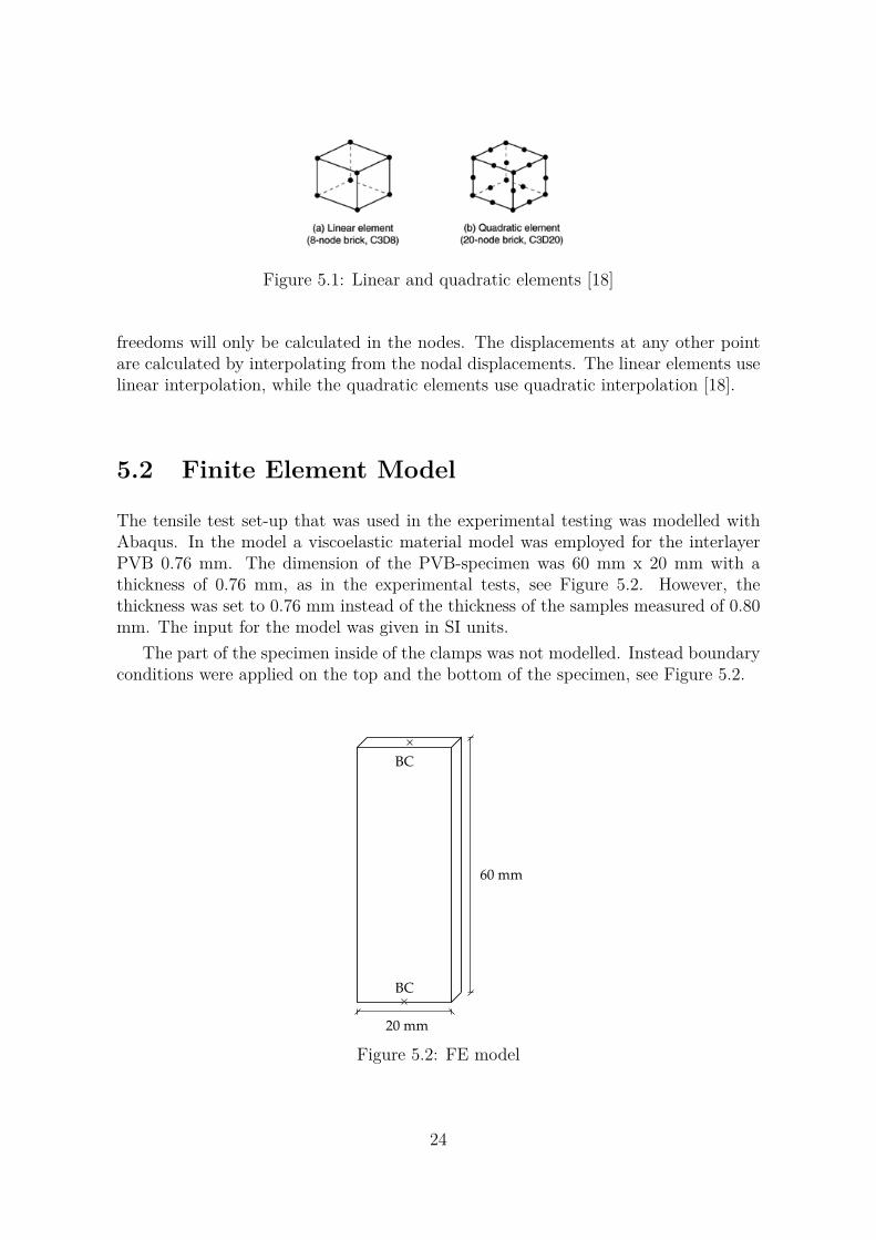
Figure 5.1: Linear and quadratic elements [18]

freedoms will only be calculated in the nodes. The displacements at any other pointare calculated by interpolating from the nodal displacements. The linear elements uselinear interpolation, while the quadratic elements use quadratic interpolation [18].

5.2 Finite Element Model

The tensile test set-up that was used in the experimental testing was modelled withAbaqus. In the model a viscoelastic material model was employed for the interlayerPVB 0.76 mm. The dimension of the PVB-specimen was 60 mm x 20 mm with athickness of 0.76 mm, as in the experimental tests, see Figure 5.2. However, thethickness was set to 0.76 mm instead of the thickness of the samples measured of 0.80mm. The input for the model was given in SI units.

The part of the specimen inside of the clamps was not modelled. Instead boundaryconditions were applied on the top and the bottom of the specimen, see Figure 5.2.

20 mm

60 mm

BC

BC

Figure 5.2: FE model

24

5.2.1 Material ModelTo obtain the viscoelastic behaviour of the PVB, the material was defined by combininglinear elasticity with viscoelasticity. The time dependent variables G(t) and E(t) arecalculated from

G(t) = G0

(1− gi

(1− e− t

τi

))(5.1)

E(t) = E0

(1− ki

(1− e− t

τi

))(5.2)

where G0 and E0 are the instantaneous shear and elastic moduli. In the elastic modelthe PVB has been defined as an isotropic material with a Young’s modulus of 2.36 MPa,a Poisson’s ratio of 0.45 and is specified for the instantaneous response, see Table 5.1.G0 is determined from E0 and ν defined in Table 5.1 using G0 = E0/2(1 + ν).

Table 5.1: Elastic parameters in Abaqus

Young’s Modulus (E0) 2.36 MPaPoisson’s Ratio (ν) 0.45Moduli Instantaneous

Viscoelasticity

The viscoelastic material parameters can be defined by inclusion of for example creeptest data, inclusion of relaxation test data or by direct specification of the Pronyseries parameters [18]. The viscoelastic properties of the PVB have been specifiedin the time domain viscoelasticity by using Prony series, see Table 5.2. The Pronyseries parameters have been determined from the experimental tensile tests data, seeSection 4.1.2. The values for ki (κi) are specified as the same as gi, see Equation 4.3and 4.4.

Table 5.2: Prony series

g_i Prony k_i Prony tau_i Prony1 0.551 0.551 32.362 0.448 0.448 4164

5.2.2 Boundary ConditionsThe specimen is in the experiment clamped in two clamps. This is realized in themodel by applying boundary conditions at the top and bottom surfaces. The boundaryconditions for the lower surface were set to zero in the x-, y- and z-direction for thetranslation (U1, U2, U3=0). For the upper surface where the specimen is drawn intension, the boundary conditions are set to zero as above, except for U2, which is setto 100% elongation (U2=0.06).

25

Figure 5.3: Mesh

5.2.3 Element Type and Mesh

The element type used in this analysis is in Abaqus denoted C3D20R. C3D20R, indi-cates it is a 3D continuum element with quadratic approximation with 20 nodes andreduced integration [18]. For the element type C3D20R the active degrees of freedomare 1, 2 and 3, meaning that Abaqus are calculating the translation in the x-, y- andz-direction in each node [18]. The element size was set to 0.001 x 0.001 m and themesh is depicted in Figure 5.3.

5.2.4 Analysis and Step

A quasi-static stress analysis was made by using the visco step. The analysis was setto take into account the non-linear effects from large displacements and deformations(geometric non-linearity) [18].

5.3 Results

From the FE model the reaction forces and displacements was plotted in MATLABand compared with the experimental results, see Figure 5.4. The data is collected fromwhere the prescribed displacement of 0.06 m is applied.

26

0 1 2 3 4 5 6

x 10−3

0

0.5

1

1.5

2

2.5

3

3.5Abaqus

Displacement [m]

For

ce [N

]

200 mm/min50 mm/min10 mm/min2 mm/min0.5 mm/min

(a) Abaqus, PVB 0.76 mm

0 1 2 3 4 5 6

x 10−3

0

0.5

1

1.5

2

2.5

3

3.5Experiment

Displacement [m]

For

ce [N

]


(b) Experiment, PVB 0.76 mm

Figure 5.4: Comparison of result

5.4 DiscussionThe result from the Abaqus-model is in good agreement with the force-displacementdiagram from the experiment, except for the load rate 200 mm/min. Even though theresult is not in good agreement with the load rate 200 mm/min, the author believesthe viscoelastic model to be valid within the limits of the strain rates performed inthe testing. The deviation is due to the test method, since the data was collected onetime per second. It is shown in Figure 5.5, that the curve for 200 mm/min followsthe curves better after 100% elongation. Please note that Figure 5.4 is expressed inforce-time, while Figure 5.5 in stress-strain.

27

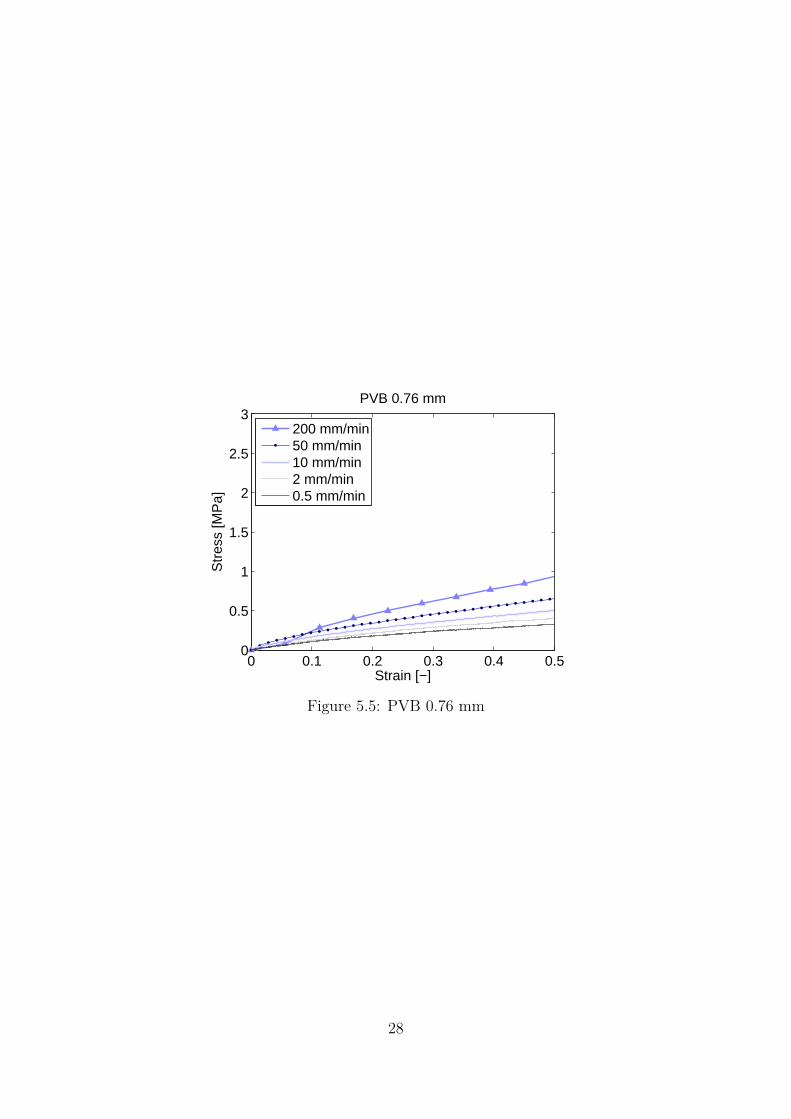
0 0.1 0.2 0.3 0.4 0.50

0.5

1

1.5

2

2.5

3PVB 0.76 mm

Strain [−]

Str

ess

[MP

a]


Figure 5.5: PVB 0.76 mm

28

Chapter 6

Numerical Application of theViscoelastic Model

The time dependency of the interlayer implemented in the viscoelastic model was de-scribed in Chapter 5. To investigate how the creep in the interlayer affects a laminatedglass unit subjected to short-term or long-term loads, a FE model was created sub-jected to various loads. An example of when laminated glass is subjected to a long-termload, such as snow load, is found for laminated glass roofs. Laminated glass facadesare on the other hand more likely designed to resist short-term wind loads instead ofsnow load. The results from the analysis of these two loading conditions show how thetime of loading affects the mechanical strength of the glass structure.

6.1 FE ModelThe study was performed on a quadratic, simply supported laminated glass unit sub-jected to uniform loading. The laminated glass unit consisted of two sheets of glassand an interlayer with the thickness 0.76 mm. The dimension of the plate was 1.5 mx 1.5 m with a thickness of 10.76 mm. Everything in the model was given in SI-units.The supports were two-sided.

The glass was modelled as a linear elastic material with isotropic properties. Thedensity was given as 2500 kg/m3 (soda-lime-silica glass) [9], the Young’s Modulus as75 GPa and the Poisson’s Ratio as 0.21, see Table 6.1.

Table 6.1: Properties of glass used in Abaqus

Density (ρ) 2500 kg/m3 [9]Young’s Modulus (E0) 75 GPaPoisson’s Ratio (ν) 0.21Moduli Long term

The interlayer was modelled as a standard PVB 0.76 mm with the material modelproposed in Section 5.2.1. The density was specified to 1070 kg/m3 to be able to applythe self-weight of the unit [9].

29

z

x

y

uz=0ux=0

uz=0

uy=0

Figure 6.1: Boundary conditions

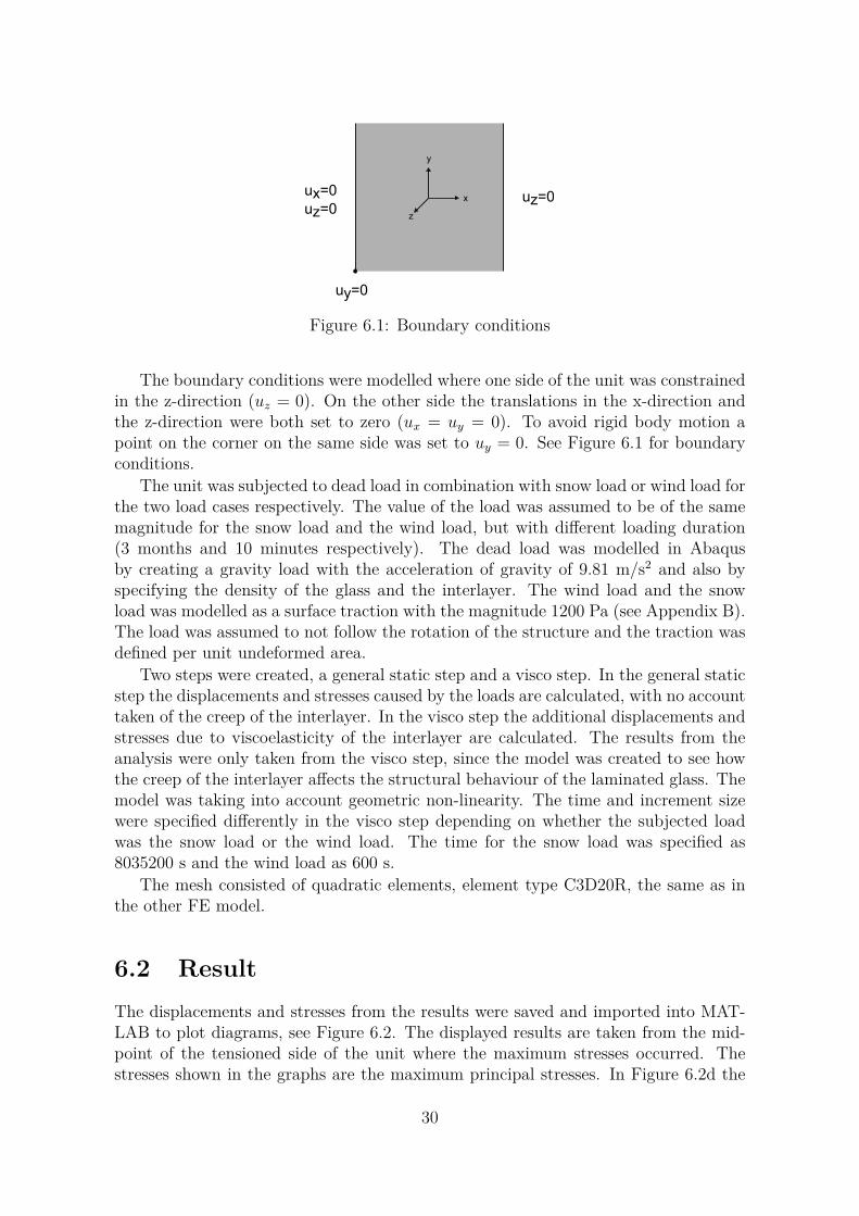
The boundary conditions were modelled where one side of the unit was constrainedin the z-direction (uz = 0). On the other side the translations in the x-direction andthe z-direction were both set to zero (ux = uy = 0). To avoid rigid body motion apoint on the corner on the same side was set to uy = 0. See Figure 6.1 for boundaryconditions.

The unit was subjected to dead load in combination with snow load or wind load forthe two load cases respectively. The value of the load was assumed to be of the samemagnitude for the snow load and the wind load, but with different loading duration(3 months and 10 minutes respectively). The dead load was modelled in Abaqusby creating a gravity load with the acceleration of gravity of 9.81 m/s2 and also byspecifying the density of the glass and the interlayer. The wind load and the snowload was modelled as a surface traction with the magnitude 1200 Pa (see Appendix B).The load was assumed to not follow the rotation of the structure and the traction wasdefined per unit undeformed area.

Two steps were created, a general static step and a visco step. In the general staticstep the displacements and stresses caused by the loads are calculated, with no accounttaken of the creep of the interlayer. In the visco step the additional displacements andstresses due to viscoelasticity of the interlayer are calculated. The results from theanalysis were only taken from the visco step, since the model was created to see howthe creep of the interlayer affects the structural behaviour of the laminated glass. Themodel was taking into account geometric non-linearity. The time and increment sizewere specified differently in the visco step depending on whether the subjected loadwas the snow load or the wind load. The time for the snow load was specified as8035200 s and the wind load as 600 s.

The mesh consisted of quadratic elements, element type C3D20R, the same as inthe other FE model.

6.2 ResultThe displacements and stresses from the results were saved and imported into MAT-LAB to plot diagrams, see Figure 6.2. The displayed results are taken from the mid-point of the tensioned side of the unit where the maximum stresses occurred. Thestresses shown in the graphs are the maximum principal stresses. In Figure 6.2d the

30

peak is reached after one day.

0 2 4 6 8 10 12−26

−25

−24

−23

−22

−21

−20

−19

−1810 Minutes

Time [min]

Dis

plac

emen

t [m

m]

(a) Displacement, 10 Min

0 20 40 60 80 100−60

−50

−40

−30

−20

−103 Months

Time [Days]

Dis

plac

emen

t [m

m]

(b) Displacement, 3 Months

0 2 4 6 8 10 1224

25

26

27

28

2910 Minutes

Time [min]

Max

Prin

cipa

l Str

ess

[MP

a]

(c) Stress, 10 Min

0 20 40 60 80 10025

30

35

40

45

503 Months

Time [Days]

Max

Prin

cipa

l Str

ess

[MP

a]

(d) Stress, 3 Months

Figure 6.2: Stresses and displacements

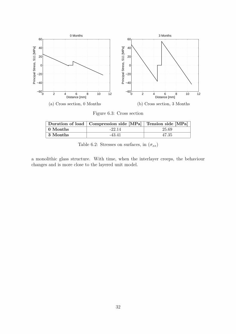
The distribution of the stresses along the cross section are depicted in Figure 6.3for the snow load. The stress in this figure is the principal stress in the x-direction(S11). Please note the differences in stresses on the compression side and the tensionside, see Table 6.2.

6.3 DiscussionIt is shown in the graphs that the stresses and displacements increase in time. Thelaminated glass subjected to snow load is more likely to be broken after three months,see Figure 6.2d. The stress is 48 MPa and according to Eurocode (prEN 16612) thecharacteristic value of the bending strength is 45 N/mm2 for annealed glass.

It is also evident that the presence of the interlayer affects the distribution of thestresses over the cross section. The duration of loading affects the distribution ofstresses. At the start of the loading, the laminated glass unit behaves more close to

31

0 2 4 6 8 10 12−60

−40

−20

0

20

40

600 Months

Distance [mm]

Prin

cipa

l Str

ess,

S11

[MP

a]

(a) Cross section, 0 Months

0 2 4 6 8 10 12−60

−40

−20

0

20

40

603 Months

Distance [mm]

Prin

cipa

l Str

ess,

S11

[MP

a]

(b) Cross section, 3 Months

Figure 6.3: Cross section

Duration of load Compression side [MPa] Tension side [MPa]0 Months -22.14 25.693 Months -43.41 47.35

Table 6.2: Stresses on surfaces, in (σxx)

a monolithic glass structure. With time, when the interlayer creeps, the behaviourchanges and is more close to the layered unit model.

32

Chapter 7

Results

The result from the experimental tests shows that there are differences in all the testedPVB. Some are stiffer, and some are softer. This shows that a PVB have variousproperties and by for example choosing a PVB with enhanced acoustic properties, themechanical strength is lowered. By the knowledge of the differences of the interlayersone can choose the most optimal interlayer for the application.

From the experimental tensile tests a viscoelastic material model can be createdto be used in simulation. The result from the FE study is in good agreement with thelaboratory results for standard PVB 0.76 mm.

The numerical application where a laminated glass unit was subjected to sustainedloads and short-term loads showed the loss in structural resistance due to the timedependent behaviour. One could note that with longer loading time, an increase inthe stresses occurs and the plate behaves more like a layered unit than a monolithicplate. This leads to the conclusion that it is important to take into account the timedependent behaviour when using laminated glass as a structural element.

However, it would be desirable to compare the FE model with the laminated glassunit with experimental results.

33

Chapter 8

Conclusions and Future Work

8.1 ConclusionsThe conclusion from the experimental tests is that PVB with various properties alsoshow different mechanical behaviour. One conclusion which also could be made duringthe study was that a viscoelastic model can be determined from tensile tests withstandard PVB 0.76 mm in good agreement with experimental results. Out of theresults gained in this report the author concludes the importance to consider the timedependent behaviour when using laminated glass as a structural element, since theincrease of stress in the laminated glass is high due to creeping in the interlayer.

8.2 Future WorkFuture work that may be done is to evaluate the other interlayers and create a Pronyserie which can be used in numerical simulations. For a more comprehensive determi-nation of the viscoelastic properties further studies may be done on the temperaturedependency of the material. It would also be of interest to compare the laminatedglass model in Abaqus with experimental research to see how good the model is. Itwould also be interesting to do shear tests with the interlayers bonded together withthe glass. The adhesion of the interlayer to the glass is also of interest when usinglaminated glass as a structural element.

35

Bibliography

[1] R.A. Behr, J.E. Minor, M.P. Linden, and C.V.G Vallabhan. Laminated GlassUnits Under Uniform Lateral Pressure. Journal of Structural Engineering, 1985.

[2] Luigi Biolzi, Emanuele Cagnacci, Maurizio Orlando, Lorenzo Piscitelli, and Gi-anpaolo Rosati. Long term response of glass-PVB double-lap joints. Composites:Part B, Elsevier, 2014.

[3] S. Briccoli Bati, G. Ranocchiai, C. Reale, and L. Rovero. Time-Dependent Be-havior of Laminated Glass. Journal of Materials in Civil Engineering, 2010.

[4] Tzikang Chen. Determining a Prony Series for a Viscoelastic Material From TimeVarying Strain Data. NASA / U.S. Army Research Laboratory, 2000.

[5] COST. COST Action TY0905 Mid-term Conference on Structural Glass. CRCPress, Leiden, The Netherlands, 2013.

[6] Tore Dahlberg. Teknisk hållfasthetslära. Studentlitteratur, Lund, 3 edition, 1990.

[7] Maria Fröling. Strength Design Methods for Glass Structures. Lund University,2013.

[8] Glasforskningsinstitutet Glafo. Boken om glas. Glafo, Växjö, 2nd edition edition,2005.

[9] Matthias Haldimann, Andreas Luible, and Mauro Overend. Structural Use ofGlass. ETH Zürich and International Association for Bridge and Structural En-gineering, Zürich, 2008.

[10] J.A. Hooper. On the Bending on Architectural Laminated Glass. InternationalJournal of Mechanical Sciences, Pergamon Press, 1972.

[11] Eric Le Bourhis. Glass; Mechanics and Technology. WILEY-VCH Verlag GmbH& Co. KGaA, Weinheim, 2008.

[12] Niels Saabye Ottosen and Hans Petersson. Introduction to the Finite ElementMethod. Prentice Hall, London, Great Britain, 1992.

[13] Michael Patterson. Structural Glass Facades and Enclosures. John Wiley & Sons,Inc., Hoboken, New Jersey, 2011.

[14] Carlson Per-Olof. Bygga med glas. Ljungbergs Tryckeri AB, 2005.

37

[15] Pilkington. The float process. http://www.pilkington.com/pilkington-information/about+pilkington/education/float+process/default.htm. Accessed2014-03-19.

[16] Vincent Sackmann. Untersuchungen zur Dauerhaftigkeit des Schubverbunds inVerbundsicherheitsglas mit unterschiedlichen Folien aus Polyvinylbutyral. Tech-nische Universität München, 2008.

[17] Albrecht Schutte and Werner Hanenkamp. Zum Tragverhalten von Verbund- undVerbundsicherheitsglas bei erhöhten Temperaturen unter Einwirkung von statis-chen und dynamischen Lasten, volume 76. Bautechnik, 1999.

[18] Dassault Systems. ABAQUS Analysis User’s Manual 6.12, 2014.

38

Appendix A

Experimental Test Results

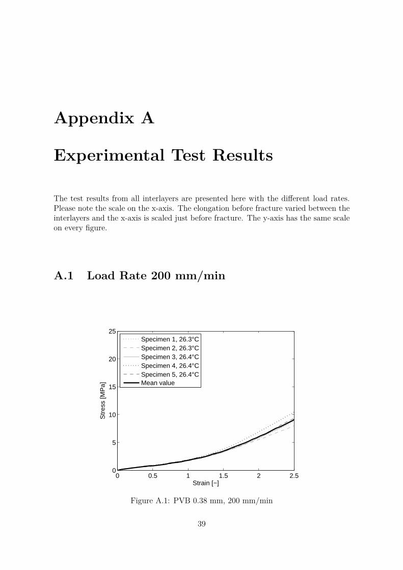
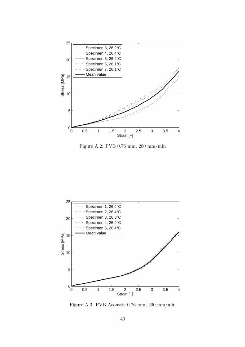
The test results from all interlayers are presented here with the different load rates.Please note the scale on the x-axis. The elongation before fracture varied between theinterlayers and the x-axis is scaled just before fracture. The y-axis has the same scaleon every figure.

A.1 Load Rate 200 mm/min

0 0.5 1 1.5 2 2.50

5

10

15

20

25

Strain [−]

Str

ess

[MP

a]

Specimen 1, 26.3°CSpecimen 2, 26.3°CSpecimen 3, 26.4°CSpecimen 4, 26.4°CSpecimen 5, 26.4°CMean value

Figure A.1: PVB 0.38 mm, 200 mm/min

39

0 0.5 1 1.5 2 2.5 3 3.5 40

5

10

15

20

25

Strain [−]

Str

ess

[MP

a]



0 0.5 1 1.5 2 2.5 3 3.5 40

5

10

15

20

25

Strain [−]

Str

ess

[MP

a]


Figure A.3: PVB Acoustic 0.76 mm, 200 mm/min

40

0 0.5 1 1.5 2 2.5 3 3.50

5

10

15

20

25

Strain [−]

Str

ess

[MP

a]


Figure A.4: DMJ1, 200 mm/min

0 0.5 1 1.5 2 2.50

5

10

15

20

25

Strain [−]

Str

ess

[MP

a]


Figure A.5: VS02, 200 mm/min

41

0 0.5 1 1.5 2 2.50

5

10

15

20

25

Strain [−]

Str

ess

[MP

a]


Figure A.6: DG41, 200 mm/min


0 0.5 1 1.5 2 2.5 30

5

10

15

20

25

Strain [−]

Str

ess

[MP

a]



42

0 0.5 1 1.5 2 2.5 3 3.5 4 4.50

5

10

15

20

25

Strain [−]

Str

ess

[MP

a]



0 0.5 1 1.5 2 2.5 3 3.5 40

5

10

15

20

25

Strain [−]

Str

ess

[MP

a]



43

0 0.5 1 1.5 2 2.5 3 3.50

5

10

15

20

25

Strain [−]

Str

ess

[MP

a]



0 0.5 1 1.5 20

5

10

15

20

25

Strain [−]

Str

ess

[MP

a]



44

0 0.5 1 1.5 2 2.50

5

10

15

20

25

Strain [−]

Str

ess

[MP

a]




0 0.5 1 1.5 2 2.5 3 3.50

5

10

15

20

25

Strain [−]

Str

ess

[MP

a]

Specimen 1, 25.1°CSpecimen 2, 25.4°CSpecimen 3, 25.4°CMean value


45

0 1 2 3 4 50

5

10

15

20

25

Strain [−]

Str

ess

[MP

a]



0 0.5 1 1.5 2 2.5 3 3.5 4 4.50

5

10

15

20

25

Strain [−]

Str

ess

[MP

a]



46

0 0.5 1 1.5 2 2.5 3 3.50

5

10

15

20

25

Strain [−]

Str

ess

[MP

a]



0 0.5 1 1.5 20

5

10

15

20

25

Strain [−]

Str

ess

[MP

a]



47

0 0.5 1 1.5 2 2.50

5

10

15

20

25

Strain [−]

Str

ess

[MP

a]



48

A.4 Load Rate 2 mm/min and 0.5 mm/min

0 0.2 0.4 0.6 0.8 10

0.2

0.4

0.6

0.8

1

Strain [�]

Str

ess [

MP

a]

PVB 0.38 mm

2 mm/min

0.5 mm/min

0 0.2 0.4 0.6 0.8 10

0.2

0.4

0.6

0.8

1

Strain [�]S

tress [

MP

a]

PVB 0.76 mm

2 mm/min

0.5 mm/min

0 0.2 0.4 0.6 0.8 10

0.2

0.4

0.6

0.8

1

Strain [�]

Str

ess [

MP

a]

PVB Acoustic 0.76 mm

2 mm/min

0.5 mm/min

0 0.2 0.4 0.6 0.8 10

0.2

0.4

0.6

0.8

1

Strain [�]

Str

ess [

MP

a]

DMJ1

2 mm/min

0.5 mm/min

0 0.2 0.4 0.6 0.8 10

2

4

6

8

10

Strain [�]

Str

ess [

MP

a]

VS02

2 mm/min

0.5 mm/min

0 0.2 0.4 0.6 0.8 10

2

4

6

8

10

Strain [�]

Str

ess [

MP

a]

DG41

2 mm/min

0.5 mm/min

Figure A.19: Load rate 2 mm/min and 0.5 mm/min for every type of interlayer

49

Appendix B

Loads

The loads are calculated according to Eurocode, SS-EN 1991-1-3.

B.1 Snow LoadThe snow load is calculated according to Eurocode 1: Actions on structures - Part 1-3:General actions - Snow loads (SS-EN1991-1-3).

s = µiCeCtsk (B.1)

whereµi is the form factor for the snow load, assumed µ1 = 0.8 (Table 5.2, 0°≤ α ≤ 30°)sk is the characteristic value of ground snow load, assumed sk = 1.5 kN/m2 (Ap-

pendix NB, Lund)Ce is the exposure factor, assumed Ce = 1.0 (Table 5.1, Normal Topography)Ct is the thermal coefficient, assumed Ct = 1.0The snow load used in simulation is

s = 0.8 · 1.5 · 1.0 · 1.0 = 1200 Pa (B.2)

A typical value for the duration of snow load is 3 Months.

B.2 Wind LoadThe wind load is assumed to be 1200 Pa as well. A typical value for the duration ofwind load is 10 Minutes. Otherwise, how to calculate the magnitude of wind loadscan be seen in Eurocode 1: Actions on structures - Part 1-4: General actions - Windactions (SS-EN 1991-1-4).

51

MECHANICAL PROPERTIES OF INTERLAYERS IN · PDF fileMaster’s Dissertation Structural...

Documents

Transcript of MECHANICAL PROPERTIES OF INTERLAYERS IN · PDF fileMaster’s Dissertation Structural...