MECH 3130: Mechanics of Materials Fall 2015 Laboratory ...htippur/mech7300-16/MECH3130-Vol2 - Fall...

1

MECH 3130: Mechanics of Materials

Fall 2015

Laboratory Manual

Volume – II

Instructor

Dr. Peter Schwartz Dr. Nels Madsen

Lab Teaching Assistants

Quang Nguyen: [email protected] Abhiram Pasumarthy [email protected]

Jing Wu [email protected] Abdullah Fahim [email protected]

2

CONTENTS

1. FINITE ELEMENT ANALYSIS OVERVIEW 3

2. ANALYSIS OF TRUSS – TUTORIAL 12

3. ANALYSIS OF TRUSS – EXERCISE 34

4. ANALYSIS OF BEAM – TUTORIAL 36

5. ANALYSIS OF BEAM – EXERCISE 45

6. 2D STRESS ANALYSIS AND SCF – TUTORIAL 46

7. 2D STRESS ANALYSIS AND SCF – EXERCISE 60

8. ANSYS-CAD INTERFACE & ANALYSIS – TUTORIAL 61

9. ANSYS-CAD INTERFACE & ANALYSIS – EXERCISE 73

3

LAB # 8 Finite Element Analysis Overview

Source: ANSYS documentation

What is Finite Element Analysis (FEA)?

Finite element method is a numerical analysis technique for obtaining approximate solutions to a

wide variety of engineering problems. Usually the problem addressed is too complicated to be

solved satisfactorily by classical analytical methods. The finite element method produces many

simultaneous algebraic equations, which are generated and solved on a digital computer. The finite

element method originated as a method of stress analysis. Today finite element methods are used

to analyze problems of heat transfer, fluid flow, lubrication, electric and magnetic fields, and many

others. Finite element procedures are used in the design of buildings, electric motors, heat engines,

ships, airframes and spacecraft.

The word finite element method was first coined by Clough in 1960 in a paper on plane elasticity

problems. In the years since 1960 the finite element method received widespread acceptance in

engineering. With the advent of the digital computer, it opened a new avenue for solving complex

plane elasticity problems. The first commercial finite element software made its appearance in

1964.

The finite element method works by discretizing (breaking a real object into a large number of

small elements). The behavior of each element is readily predicted by set mathematical equations.

Then the computer adds up all the individual behaviors to predict the overall behavior of the actual

object. The word "finite" in finite element analysis comes from the idea that there are finite

numbers of elements in a model. This is in contrast to the classical approach (differential equation

method) where an infinitesimal element is considered for derivation of the governing equations.

To summarize, the finite element method satisfies the governing equations in an approximate or

average sense whereas classical methods insist on validity of the solution at each and every point

in the domain. The finite element method is employed to solve almost all physical systems.

Structural mechanics (stress analysis)

Mechanical vibration

Heat transfer - conduction, convection, radiation

Fluid Flow - both liquid and gaseous fluids

4

Various electrical and magnetic phenomena

Acoustics

What is a Node?

A node is a coordinate location in space where the degrees of freedom (DOF) are defined. In the

context of stress analysis of structural members, the DOF represent the possible motion of a point

due to loading of the structure. The forces and moments are transferred between two adjacent

elements through a node.

What is an Element?

An element is the basic building block of a finite element model. There are several basic types of

elements. Typically, an element is bounded by the nodal points. Examples are solid brick and

tetrahedron elements for 3 dimensional problems, Quadrilateral and triangular elements for 2

dimensional problems, beam and truss elements are typical line elements. Also the elements may

be straight in shape or curved.

Some General Type of Elements in ANSYS:

1. LINK 1 (or 2-D Spar or Truss):

“LINK 1” is the ANSYS name of the element.

“2-D Spar or Truss” is the type of the element.

LINK1 can be used in a variety of engineering applications. Depending upon the application,

you can think of the element as a truss, a link, a spring, etc. The 2-D spar element is a uniaxial

tension-compression element with two degrees of freedom at each node: translations in the

nodal x and y directions. As in a pin-jointed structure, no bending of the element is considered.

5

LINK1 Input Summary:

Nodes : I, J

Degrees of Freedom : UX, UY

Real Constants : AREA - Cross-sectional area

ISTRN - Initial strain

Material Properties : EX (Young/s Modulus), PRXY (Poisson’s Ratio)

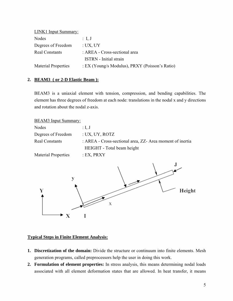
2. BEAM3 ( or 2-D Elastic Beam ):

BEAM3 is a uniaxial element with tension, compression, and bending capabilities. The

element has three degrees of freedom at each node: translations in the nodal x and y directions

and rotation about the nodal z-axis.

BEAM3 Input Summary:

Nodes : I, J

Degrees of Freedom : UX, UY, ROTZ

Real Constants : AREA - Cross-sectional area, ZZ- Area moment of inertia

HEIGHT - Total beam height

Material Properties : EX, PRXY

Typical Steps in Finite Element Analysis:

1. Discretization of the domain: Divide the structure or continuum into finite elements. Mesh

generation programs, called preprocessors help the user in doing this work.

2. Formulation of element properties: In stress analysis, this means determining nodal loads

associated with all element deformation states that are allowed. In heat transfer, it means

6

determining nodal heat fluxes associated with all element temperature fields that are allowed.

3. Assembly procedure: Assemble elements to obtain the global finite element model of the

structure.

4. Apply loads: These are nodal forces and/or moments in stress analysis, nodal heat fluxes in

heat transfer analysis.

5. Impose boundary conditions: In stress analysis, specify how the structure is supported. This

step involves setting several nodal displacements to known values (which are often zeros). In

heat transfer, where typically certain temperature are known, impose all known values of

temperatures.

6. Solution: Solve simultaneous linear algebraic equations to determine nodal degrees of freedom

(Nodal displacements in stress analysis, nodal temperatures in heat transfer analysis).

7. Post Processing: In stress analysis, calculate element strains from the nodal degrees of

freedom and the element displacement field interpolation, and calculate stresses from strains.

Finally calculate additional quantities like strain energy, von-mises stress, etc. In heat transfer,

calculate element heat fluxes from the nodal temperatures and the element temperature filed

interpolation. Output interpretation programs, called Postprocessors, help the user sort the

output and display it in graphical form.

Introduction to ANSYS:

ANSYS finite element analysis software enables engineers to perform the following tasks:

Build computer models or transfer CAD models of structures, products, components, or

systems.

Apply operating loads or other design performance conditions.

Study physical responses, such as stress levels, temperature distributions, or electromagnetic

fields.

Optimize a design early in the development process to reduce production costs.

Do prototype testing in environments where it otherwise would be undesirable or impossible

(for example, biomedical applications).

The ANSYS program has a comprehensive graphical user interface (GUI) that gives users easy,

interactive access to program functions, commands, documentation, and reference material. An

intuitive menu system helps users navigate through the ANSYS program. Users can input data

using a mouse, a keyboard, or a combination of both.

7

Overview of Model Generation:

What Is Model Generation?

In ANSYS terminology, the term model generation usually takes on the narrower meaning of

generating the nodes and elements that represent the spatial volume and connectivity of the actual

system. Thus, model generation in this discussion will mean the process of defining the geometric

configuration of the model's nodes and elements. The ANSYS program offers you the following

approaches to model generation:

Creating a solid model within ANSYS.

Using direct generation.

Importing a model created in a computer-aided design (CAD) system.

Typical Steps Involved in Model Generation within ANSYS:

Begin by planning your approach. Determine your objectives, decide what basic form your

model will take, choose appropriate element types, and consider how you will establish an

appropriate mesh density. You will typically do this general planning before you initiate your

ANSYS session.

Enter the preprocessor (PREP7) to initiate your model-building session. Most often, you will

build your model using solid modeling procedures.

Establish a working plane.

Generate basic geometric features using geometric primitives and Boolean operators.

Activate the appropriate coordinate system.

Generate other solid model features from the bottom up. That is, create key points, and then

define lines, areas, and volumes as needed.

Use more Boolean operators or number controls to join separate solid model regions together

as appropriate.

Create tables of element attributes (element types, real constants, material properties, and

element coordinate systems).

Set element attributes pointers.

Create nodes and elements by meshing your solid model.

Save your model data to Jobname.DB, and exit the preprocessor.

8

Importing Solid Models Created in CAD systems:

As an alternative to creating your solid models within ANSYS, you can create them in your

favorite CAD system and then import them into ANSYS for analysis, by saving them in the IGES

file format or in a file format supported by an ANSYS Connection product. Creating a model using

a CAD package has the following advantages:

Planning Your Approach:

As you begin your model generation, you will (consciously or unconsciously) make a number of

decisions that determine how you will mathematically simulate the physical system: What are the

objectives of your analysis? Will you model all, or just a portion, of the physical system?

How much detail will you include in your model? What kinds of elements will you use? How

dense should your finite element mesh be? In general, you will attempt to balance computational

expense (CPU time, etc.) against precision of results as you answer these questions. The decisions

you make in the planning stage of your analysis will largely govern the success or failure of your

analysis efforts.

Determine Your Objectives:

This first step of your analysis relies not on the capabilities in the ANSYS program, but relies

instead on your own education, experience, and professional judgment. Only you can determine

what the objectives of your analysis must be. The objectives you establish at the start will influence

the remainder of your choices as you generate the model.

Your finite element model may be categorized as being 1-Dimensional, 2-dimensional or 3-

dimensional, and as being composed of point elements, line elements, area elements, or solid

elements. Of course, you can combine different kinds of elements as required (taking care to

maintain the appropriate compatibility among degrees of freedom). For example, you might model

a stiffened shell structure using 3-D shell elements to represent the skin and 3-D beam elements to

represent the ribs. Your choice of model dimensionality and element type will often determine

which method of model generation will be most practical for your problem.

LINE models can represent 2-D or 3-D beam or pipe structures, as well as 2-D models of 3-D

axisymmetric shell structures. Solid modeling usually does not offer much benefit for generating

line models; they are more often created by direct generation methods.

9

2-D SOLID analysis models are used for thin planar structures (plane stress), "infinitely long"

structures having a constant cross section (plane strain), or axisymmetric solid structures. Although

many 2-D analysis models are relatively easy to create by direct generation methods, they are

usually easier to create with solid modeling.

3-D SHELL models are used for thin structures in 3-D space. Although some 3-D shell analysis

models are relatively easy to create by direct generation methods, they are usually easier to create

with solid modeling.

3-D SOLID analysis models are used for thick structures in 3-D space that have neither a constant

cross section nor an axis of symmetry. Creating a 3-D solid analysis model by direct generation

methods usually requires considerable effort. Solid modeling will nearly always make the job

easier.

Coordinate Systems:

The ANSYS program has several types of coordinate systems, each used for a different reason:

Global and local coordinate systems are used to locate geometry items (nodes, key points, etc.)

in space.

The display coordinate system determines the system in which geometry items are listed or

displayed.

The nodal coordinate system defines the degree of freedom directions at each node and the

orientation of nodal results data.

The element coordinate system determines the orientation of material properties and element

results data.

The result coordinate system is the coordinate system in which results are computed and

displayed.

What Are Loads?

The word ‘loads’ in ANSYS terminology includes boundary conditions and externally or internally

applied forcing functions.

Structural: displacements, forces, pressures, temperatures (for thermal strain), gravity.

Thermal: temperatures, heat flow rates, convections, internal heat generation, infinite surface.

Magnetic: magnetic potentials, magnetic flux, magnetic current segments, source current density,

infinite surface.

10

Electric: electric potentials (voltage), electric current, electric charges, charge densities, infinite

surface.

Fluid: velocities, pressures.

Solution:

What Is Solution?

In the solution phase of the analysis, the computer takes over and solves the simultaneous set of

equations that the finite element method generates. The results of the solution are:

Nodal degree-of-freedom values, which form the primary solution and Derived values, which form

the element solution.

An Overview of Post processing:

What Is Post processing?

After building the model and obtaining the solution, you will want answers to some critical

questions: Will the design really work when put to use? How high are the stresses in this region?

How does the temperature of this part vary with time? What is the heat loss across this face of my

model? How does the magnetic flux flow through this device? How does the placement of this

object affect fluid flow? The postprocessors in the ANSYS program can help you answer these

questions and others. Post processing means reviewing the results of an analysis. It is probably the

most important step in the analysis, because you are trying to understand how the applied loads

affect your design, how good your finite element mesh is, etc.

Two postprocessors are available to review your results: POST1, the general postprocessor, and

POST26, the time-history postprocessor. POST1 allows you to review the results over the entire

model at specific load steps and sub steps (or at specific time-points or frequencies). In a static

structural analysis, for example, you can display the stress distribution for load step 3. Or, in a

transient thermal analysis, you can display the temperature distribution at time = 100 seconds.

POST26 helps user to go over all the load steps at a time and observe the variation of quantities

with respect to time or frequency.

11

ANSYS Menu Overview:

The above figure shows the typical ANSYS menu. ANSYS main is divided into preprocessor,

solution, post processor etc. Some of the frequently used options are available in ANSYS pull

down menu as well. Any action that is executed through these menus can also be performed by

typing an equivalent command in the command window. The Pan-Zoom-Rotate menu facilitates

easy visualization of the model in the graphics window.

Note: Save all your work until you get your final grade in your H: drive space. You may be asked

anytime to show your work before the final grading time.

12

LAB # 8

Analysis of Truss - Tutorial

The goal of this tutorial is to guide you through the development of a finite element model for a

practical two-dimensional bridge truss structure. The geometry of the bridge is shown above. The

bridge is constructed from steel members with three unique cross sectional areas (denoted 1, 2, 3,

see Fig. 3). The areas are A1 = 13 cm2, A2 = 42 cm2, A3 = 20 cm2. The bridge is considered to be

loaded by a 3000 kg automobile as it traverses the span from one side to the other. The truss

members will be assumed to be weightless.

13

Cross sectional area: 1 : 13 cm2

2 : 42 cm2

3 : 20 cm2

Boundary Conditions: Node N1 and N5 : Ux = Uy = 0.

14

Problem statement:

Solve the above 2-dimensional truss problem using ANSYS to compute the following:

1. Displacements (Ux and Uy) at all joints (nodes) of the truss in the horizontal and vertical

directions.

2. Support reactions at the joints wherever the structure is supported.

3. Forces in each member (element).

4. Strain in each element.

5. Stress in each element.

6. Whether the structure is capable of withstanding the load?.

7. Where does the maximum displacement occur?.

8. Which element is stressed most?

Data:

1. Dimensions of the truss and cross sectional area are given above.

2. Boundary conditions are as shown in the Fig. 3.

3. Material properties:

Young’s modulus (E) = 211 GPa

Poisson’s ratio (υ) = 0.3

Yield strength = 390 MPa

15

How to save image files for use in a lab report:

To save any picture which is visible at that instance on ANSYS graphics window follow these

guidelines:

In Ansys pull down menu click PlotCtrls. Then click on Hard Copy… It will open a little window

titled PS Hard Copy. Check following options:

Graphics window, Color, JPEG, Landscape and then in Save to option type the file name as

‘filename.JPG’. You can give any file name you want. This will save the picture currently being

displayed on graphics window in .jpg format in your current working directory.

How to save text files for use in a lab report:

To save any text file which is on current displays (text files show words and numbers). Click on

‘file’. Then click on ‘save as’. Then in file name type ‘filename.txt’. You can give any name

instead of filename to save the text file. Later you can even pull the file out on windows. To open

file on window open file with “ WordPad’ ( right click on file icon then ‘open with..’ and then

select word pad. That will show you formatted output).

General guidelines for solving the problem in ANSYS:

1. Open ANSYS window

2. Geometric Modeling

Create Key points

Create Lines

Create areas

Create volumes

3. Finite element modeling

Declare analysis type

Define element type

Define the key options (e.g., Plane stress, plane strain, axisymmetric)

Define element properties (real constants, e.g., thickness, area of cross section)

Define material properties (e.g., E, υ, ρ etc.)

Create nodes and elements (Meshing)

Merge items (if there is any overlapping among the entities)

16

4. Solution

Specify analysis type

Apply boundary conditions (i.e., fixing the structure)

Apply loads

Specify the solution parameters

Solve the problem

5. Post processing

Get the displacements, reaction forces, strains and stresses.

Plot the output variables if needed.

Caution:

ANSYS does not make any distinction between units. It is the user’s responsibility to use correct

and consistent units while solving the problem. If inconsistent units are used, the solution will be

WRONG. For example, if the model is in meter, Young’s modulus must be in N/m2 and forces will

be in Newton, Pressure (if applied) will be in Pascal, mass density in kg/m3 etc. Similarly if model

is in inches, then E in psi, loads are in lb(f) etc.

Step by step procedure to solve the truss problem using ANSYS:

a) Open ANSYS window:

1. Log on to system, and open up Ansys.

2. Change the Simulation environment to Ansys.

3. Set the working directory as your username/fea/truss/tutorial.

4. Type “tutorial” in the menu Job Name as shown in Fig. 6.

5. Click on “run”.

17

Figure 6

b) Geometric modeling:

Creating Key Points:

1. File – Change title

2. Type “ Two dimensional truss problem”

3. OK

4. Preprocessor

5. Modeling

6. Create

7. Keypoints

8. On working plane

9. Type the following numbers in ANSYS input window (Press enter key after typing each

coordinate. Note the values are in meter.)

0, 0

2.5, 0

5.0, 0

18

7.5, 0.0

10.0, 0.0

1.25, 1.25

2.5, 1.25

5.0, 1.25

7.5, 1.25

8.75, 1.25

10. OK

11. File – Save as Jobname.db …

Creating Lines:

12. Modeling – Create – Lines – Lines

13. Straight Line

14. Go on clicking on start point and end point until you get the desired geometry. (You can

unselect any point by clicking right button of the mouse and reselect by clicking left

button.)

15. OK

c) Finite Element Modeling:

Declare analysis type:

1. Main menu

2. Preferences

3. Structural (as shown in Fig. 8)

4. OK

19

Define element type:

5. Preprocessor

6. Element type

7. Add/Edit/Delete

8. Add

9. Link 3D finit stn 180 (as shown in Fig. 9).

10. OK

11. Close

Define Element properties (real constants for truss element):

12. Real constants

13. Add/Edit/Delete

14. Add

15. OK

16. Type 0.0013 in the Field AREA as shown in Fig. 10.

17. OK

18. Add

19. OK

20

20. Type 0.0042

21. OK

22. Add

23. OK

24. Type 0.002

25. OK

26. Close

Figure 9

Figure 10

21

Define Material properties:

27. Preprocessor

28. Material Props

29. Material Models

Structural

Linear

Elastic

Isotropic

EX 211e9 (this is Young’s modulus)

PRXY 0.3 (this is Poisson’s Ratio)

OK

Close the window

Create nodes and Elements (Meshing of Rod elements):

30. Preprocessor – Meshing – Mesh Tool

31. Size Controls: Lines - Set (See Fig. 11)

32. Pick all

33. Ndiv No of Element divisions (enter 1) (see Fig. 11)

34. OK

35. Mesh Attributes

36. Picked Lines

37. Pick all the lines with cross sectional area 13 cm2 (refer page 12).

38. OK

22

Figure 11

39. Check the following attributes for the elements: (Fig. 12)

MAT, Material number =1,

REAL, Real constant set number = 1,

TYPE, Element type number = 1

40. OK

41. Mesh

42. Click on the lines with cross sectional area 13 cm2

43. OK

44. Plot

23

45. Multi-Plots

46. PlotCtrls

47. Numbering

48. Check the Node numbers on (see Fig. 13)

49. Check the Element numbers on in Elements/Attrib numbering (see Fig. 13)

50. OK

51. Repeat the steps from 35 to 45.This time select the lines having cross sectional area of 42

cm2. Assign the REAL, Real constant set number = 2.

Figure 12

24

Figure 13

52. Repeat steps from 35 to 45. This time select the lines having cross sectional area of 20 cm2.

Assign the REAL, Real constant set number = 3.

53. Type the command elist in the Command window and pay attention to Fig. 14 and note

that following are present in your model.

1 thru 17 3D truss elements (link elements)

All elements are of material type 1

Elements 1 thru 8 are having cross sectional area of 13 cm2



54. Type the commands rlist to verify the cross sectional areas you have specified are indeed

present.

55. Type the command mplist to verify the material properties you have specified are indeed

present.

25

Figure 14

d) Solution:

Specify analysis type:

56. Solution

57. Analysis Type

58. New Analysis

59. Static

60. OK

Specify solution parameters:

61. Sol’n Controls

62. Check the following items in the Basic sub menu of solution controls dialog box as shown

in Fig.15.

26

Analysis options - Small displacement static

Time at end of load step – 1

Write items to result file – All solution items

63. OK

Figure 15

Apply Boundary conditions:

64. Solution

65. Define Loads

66. Apply

67. Structural

68. Displacement

69. On Nodes

70. Click on node number 1 and 5 (Bottom left and bottom right nodes)

71. OK

72. Check on “All DOF” (As shown in Fig. 16).

73. OK (A horizontal and a vertical triangle appears indicating that the node is fixed both in x

and y directions.)

27

Figure 16

Apply Loads:

74. Solution

75. Define Loads

76. Apply

77. Structural

78. Force/Moment

79. On Nodes

80. Click on Node no 2

81. OK

82. Check “FY” for Direction of Force/Moment and type a value of -30000 (as shown in Fig.

17 – This is the total weight of the vehicle W (N) = m (kg)*g (m/sec2) = 3000*10 = 30000

N, -ve sign indicates the load is acting downwards).

83. OK

84. Load Step Opts

85. Write LS File

86. Type the number 1 in the field LSNUM

87. OK

88. Define Loads

89. Delete

28

90. Structural

91. Force/Moment

92. On Nodes

93. Click on Node Number 2 (Note: see node figure in problem statement and then click on

your model on that corresponding node , in your model the number might be different)

94. OK

95. Check “ALL” in the Lab field

96. OK

97. Repeat the steps 75 to 87 with the following changes:

Vertical load of -30000 N to be applied on Node no 3

Type the number 2 instead of 1 in step 86.

98. Now delete all the previous loads and ( follow steps 88-96)

99. Repeat the steps 75 to 87 with the following changes:

Vertical load of -30000 N to be applied on Node no 4

Type the number 3 instead of 1 in step 86.

100. File – Save as Jobname.db

Note: Here you have created 3 load steps for 3 different positions of car on the bridge,

i.e. on left side of bridge, in the middle and on right side of bridge and then you’ll solve

for all 3 positions one by one.

Figure 17

Solving the problem:

101. Solution

102. Solve

103. From LS Files ( Note:LS stands for Load Step )

104. Type 1, 3 and 1 for LSMIN, LSMAX and LSINC respectively as shown in Fig. 18.

29

105. OK

106. You are OK if you get a dialog box “Solution is Done”. Otherwise contact instructor.

Figure 18

e) Post Processing the Results:

Read the result file and plot the deformed shape:

107. General Postproc

108. Data & File Opts

109. Check on “All items”, Click on “…” and select the file, “tutorial.rst” as shown in Fig.

19.

110. OK

111. Read Results

112. First Set

113. Plot Results

114. Deformed Shape

115. Check on “Def + undeformed”

116. OK

117. This gives the deformed shape overlapped on undeformed shape for load case 1 (Save it

as a picture: Plotctrls - Hard Copy - To File – Save to - <file.bmp> )

118. Read Results - Next Set and repeat steps 113-115.

119. Read Results - Last set and repeat steps 113-115.

30

Figure 19

Check the reactions:

120. List Results

121. Reaction Solu

122. Check on All items

123. OK

124. Verify whether the reactions are summing up to give the applied load in vertical direction

and zero in horizontal direction (This is an important check).

Plot displacements:

125. Read Results – First Set

126. Plot Results – Contour Plot

127. Nodal Solu

128. Check on “DOF Solution” and “y – component of displacement”

129. OK (Compare your plot Fig. 21)

130. Save this picture.

131. Plotctrls - hard copy - to file – select the format you wish - save to - <file.bmp>

132. OK (The pictures will be stored in the current working directory).

31

Figure 20: Deformed Vs Undeformed plot

Figure 21: Vertical displacement (Uy) of the Truss

List Nodal displacements, Element forces, stresses and strains:

133. List Results

134. Nodal Solution

135. Check on “DOF Solution” and and “Displacement vector sum”

136. OK (Compare your results with those in Fig. 22)

137. Save this file for future reference (File – Save as – <filename.txt>).

138. List Results

139. Nodal Loads

140. Check on “All struc forc F”

141. OK (Compare your results with those in Table 1).

142. List Results

143. Element Solution

144. Check on “Line Elem Results” and “Element Results”

145. OK. Stresses and Strains in Element coordinate system will be listed in this file (FORCE:

axial force in each truss; STRESS: axial stress in each truss. Positive sign of STRESS

means tension and negative compression). See Fig. 23 (Save this file for future reference:

File – Save as - <filename.txt>)

Animation:

146. PlotCtrls

147. Animate

148. Deformed Results

32

149. Check on “DOF” Solution and “UY”

150. OK

Exit:

151. SAVE_DB

152. File – Exit (Quit No Save! OK)

Figure 22: Nodal displacements.

33

PRINT F REACTION SOLUTIONS PER NODE ***** POST1 TOTAL REACTION SOLUTION LISTING ***** LOAD STEP= 0 SUBSTEP= 1 TIME= 1.0000 LOAD CASE= 0 THE FOLLOWING X,Y,Z SOLUTIONS ARE IN THE GLOBAL COORDINATE SYSTEM NODE FX FY FZ 1 22500. 22500. 0.0000 5 -22500. 7500.0 0.0000 TOTAL VALUES VALUE -0.72760E-11 30000. 0.0000

TABLE 1

PRINT ELEM ELEMENT SOLUTION PER ELEMENT ***** POST1 ELEMENT SOLUTION LISTING ***** LOAD STEP 0 SUBSTEP= 1 TIME= 1.0000 LOAD CASE= 0 EL= 1 NODES= 1 2 MAT= 1 XC,YC,ZC= 1.250 0.000 0.000 AREA= 0.13000E-02 LINK180 FORCE= 0.23792E-10 STRESS= 0.18301E-07 EPEL= 0.86736E-19

TEMP= 0.00 0.00 EPTH= 0.0000

Understanding the line element results: EL= 1 element number is 1 NODES= 1 2 nodes 1 and 2 make up element 1 STRESS = 0.18301E-07 axial stress in element 1 made of nodes 1 and 2

34

LAB # 9

ANALYSIS OF TRUSSES - Exercises 1.

The truss, shown in Fig. 1, is made of AL6061-T6. Use E=10e6 psi and Poisson’s ratio =

0.35. Assume a cross-sectional area of 1” for the outer elements (shown by thicker lines)

and ½” for the diagonal elements. (All dimensions in Fig. 1 are in inches). Find the values

of axial stresses in each member of the truss using ANSYS package. Repeat your stress

calculations for the truss by hand and provide an element-by element comparison with Part-

(a).

a) Show a picture showing the loads and boundary conditions on which the element numbers

are shown.

b) Show a picture showing the deformed and undeformed shapes

c) Show a picture of the undeformed shape on which the corresponding stress values of each

link are hand written beside the links.

d) Present the complete hand calculation that you did to find the stress values.

e) Present a table comparing the Ansys and hand calculated results. Use the same element

numbers in the first picture as reference.

35

2. Find the values of axial stresses in each member of the truss shown in Figure 2. Also find

displacements at each node. List the values of the maximum displacement and axial stress in

the truss. Consider the following material and sectional properties to analyze the truss: Young’s

modulus of all elements: 13.6e6 psi. Poisson’s ratio is 0.35. Each member along

AB,CB,AC,BE,BF ,FE,HL( Shown by thick line) has hollow circular cross section With 4.5

inch outer diameter and 2.4 inch inner diameter. Each linking element (shown by thin lines)

has solid circular cross-section with diameter 2 inch.

Note: Use same type of element as tutorial problem for both these exercise problems

a) Show a picture showing the loads and boundary conditions on which the element numbers

are also shown.

b) Show a picture showing the deformed and undeformed shapes

c) Show a picture of the undeformed shape on which the maximum axial stress value and the

maximum y – displacement value are hand written beside the respective link and node.

Note: Do not submit any numerical printed results that are directly output from Ansys.

36

LAB # 10 Analysis of Beam - Tutorial

Analysis of a Bicycle Handlebar

Analyze the bicycle handle bar shown in the Figure 1 (i) without and (ii) with the reinforcement

bar. For both cases find maximum stresses in each of the members and deflections at the end of

the handle. Find the value of maximum stress and its location. Consider the followings while

analyzing the model:

a) Each member of the handle has hollow circular section with 3/4” outer diameter and thickness

1/8”.

b) The reinforcing bar has a hollow circular cross section with outer diameter ½” and thickness

1/8”.

c) Consider the material as steel with Young’s modulus 30E6 psi and Poisson’s ratio 0.3.

d) Assume a distributed load of 100 lb(f) over the shaded regions of the handle.

Note: In this tutorial, the problem is solved with the reinforcement bar. You need to solve without

the reinforcement bar and compare the results in the lab.

37

Step by step procedure to solve the beam problem using ANSYS:

1. Open Ansys in the working directory named “Tutorial” under “Beam”.

a) Geometric modeling:

Creating key points:


3. Type “Analysis of Bicycle handlebar using 2D beam element”

4. OK

5. Preprocessor

6. Modeling

7. Create

8. Key points

9. On Working Plane

10. Type the following numbers in ANSYS input window(Press enter key after typing each

number)

0,0

4,0

6,0

9,-5.196

12,-5.196

15,-5.196

18,0

20,0

24,0

12,-6.196

7.039,-1.8

16.961,-1.8

11. OK

12. Save the file

38

Creating Lines:

13. Lines – Lines

14. Straight line

15. Go on clicking on start point and end point until you get the desired geometry (You can

unselect any point by clicking right button of the mouse)

16. OK (Make sure that you got the geometry shown in Fig. 2.


b) Finite element modeling:


18. Main Menu

19. Preferences

20. Structural

21. OK

Define element type :

22. Preprocessor

23. Element Type

24. Add/Edit/Delete

25. Add

39

26. Beam 2 node 188 (as Shown in Fig. 3.) (OR type command: et, 1, BEAM188 in –

command window) The selection must be displayed in selection display bar.

27. OK

28. Close

Define Element properties (real constants for beam element):

29. Preprocessor

30. Sections

31. Beam

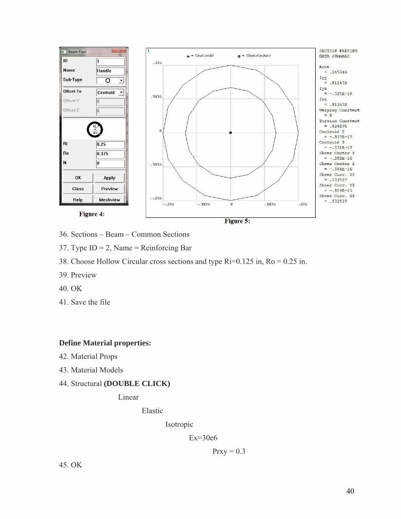
32. Common Sections (a beam tool appears as shown in Fig. 4).

33. Type “Handle” in the Name section, Chose Hollow Circular cross sections

and type 0.25 in for inner radius and 0.375 in for outer radius. Leave ‘N’ blank.

34. Preview (Beam cross sectional properties appear as shown in Fig. 5).

35. OK

40

36. Sections – Beam – Common Sections

37. Type ID = 2, Name = Reinforcing Bar

38. Choose Hollow Circular cross sections and type Ri=0.125 in, Ro = 0.25 in.

39. Preview

40. OK

41. Save the file


42. Material Props

43. Material Models

44. Structural (DOUBLE CLICK)

Linear

Elastic

Isotropic

Ex=30e6

Prxy = 0.3

45. OK

41

46. Material – Exit

47. Save the file

48. Plot – Multi-Plot

Create nodes and Elements (Meshing):

49. Select

50. Entities

51. Check the following items

Lines

By Num/Pick

From Full

OK (Expand window if you don’t see OK button).

52. Mouse pick all the lines except reinforcement bar (long one)

53. OK

54. Select – Everything Below – Selected Lines

55. Plot - Lines


57. Click on Lines Set

58. Pick all

59. Type 5 in NDIV field

60. OK (This is called mesh seeding)

61. Preprocessor – Meshing – Mesh Attributes – Picked lines – Pick all

62. Check the following items and click OK.

Material number 1

Element type number 1 BEAM188

Element section 1 Handle

63. Mesh (on Mesh Tool window. Sometimes Mesh Tool window is hidden behind the main

window and can be found by restoring down the main window)

64. Pick all (This is called meshing)

65. Select - Everything

66. Plot – Multi-Plots

42

67. Repeat the steps from 49 to 55 by selecting only reinforcement bar

68. Repeat the steps from 57 to 60 by typing 10 in NDIV field for reinforcement

bar

69. Repeat 61 to 66 by assigning Element

section = Reinforcement bar

70. Select – Everything

71. Plot – Elements


d) Solution:


73. Solution – Analysis Type – New Analysis – Static

74. OK

75. Sol’n Controls (all defaults)

76. OK


77. Solution – Define Loads – Apply – Structural – Displacement – On Nodes

78. Pick the bottom most node of the supporting rod

79. OK

80. Check on “All DOF”

81. OK

Apply Loads:

82. Solution – Define Loads – Apply – Force/Moment – On Nodes

83. Select (6+6 =12) nodes on the handle (6 on each end. Show nodes by clicking Plot-Nodes

and select 6 nodes starting from very left (right) on each handle).

84. OK

85. Select FY in the field Lab and type a value of -8.33 in the field VALUE (Note: 100 lb

load is uniformly distributed on 12 nodes (8.33 x 12 = 100).).

86. OK (Compare your model with the one in Fig. 6).


43

Figure 6:

Solve the problem:

88. Solution

89. Solve

90. Current LS

91. OK

e) Post Processing the results:

Read the results file and Plot the deformed shape:

92. General Postproc

93. Data & File Opts

94. Highlight on All Items

95. Click … bottom – Select Jobname.rst – Open – OK


97. Plot Results – Deformed Shape (Check on Def + undeformed)

98. OK

99. To save this as a file to be included in report, do the following:

100. Plot Ctrls – Hard Copy – To File

101. Check on Color, Tiff, Tiff compression, Reverse Video, Portrait

102. OK (Compare your plot with the one in Fig. 7)

44

Figure 7:

Check reactions

103. List Results – Reaction Solu (Check on All Items)

104. OK (Verify whether the summation of vertical reactions equal to the applied

load.

Plot displacements

105. General PostProc – Plot Results – Contour Plot – Nodal Solu

106. Check on DOF Solution and y-component of displacement

Animation

118. PlotCtrls – Animate – Deformed Results

119. Check on DOF Solution and UY

120. OK

45

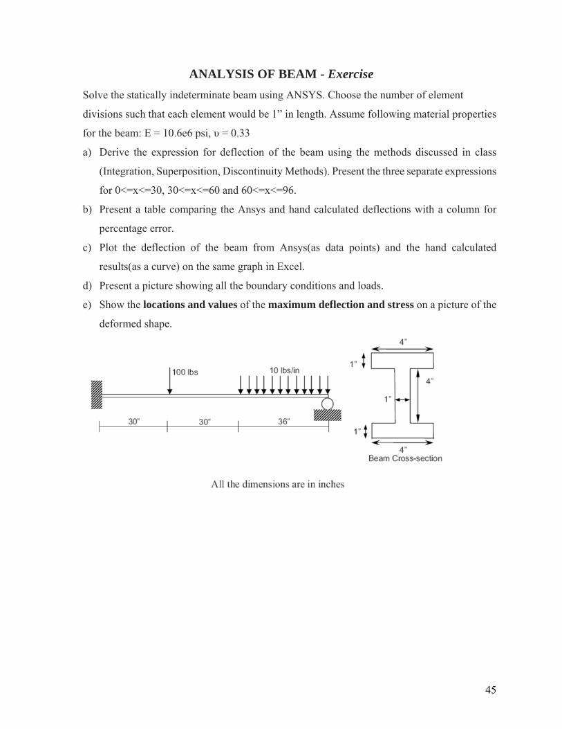
ANALYSIS OF BEAM - Exercise

Solve the statically indeterminate beam using ANSYS. Choose the number of element

divisions such that each element would be 1” in length. Assume following material properties

for the beam: E = 10.6e6 psi, υ = 0.33

a) Derive the expression for deflection of the beam using the methods discussed in class

(Integration, Superposition, Discontinuity Methods). Present the three separate expressions

for 0<=x<=30, 30<=x<=60 and 60<=x<=96.

b) Present a table comparing the Ansys and hand calculated deflections with a column for

percentage error.

c) Plot the deflection of the beam from Ansys(as data points) and the hand calculated

results(as a curve) on the same graph in Excel.

d) Present a picture showing all the boundary conditions and loads.

e) Show the locations and values of the maximum deflection and stress on a picture of the

deformed shape.

46

Lab # 11 2D Stress Analysis – Tutorial

(A note on stress concentration factor)

In engineering practice, the interest is always to know what is the value of maximum stress

occurring for given loading and given structural member geometry. Complex stress

distribution occurs near the point of load application, at locations where member’s cross

sectional area changes and more severely where, there is a defect like a crack. Figure (b) and

(c) shows the actual and average stress distribution across the cross section passing through

the hole (consider the hole as a defect here in a uniaxial test specimen). It is clear that stress at

the boundary of hole (top and bottom) is more than the average stress. The results of this kind

of investigation are usually reported in terms of ‘Stress Concentration Factor’ (SCF) K. We

define K as a ratio of the maximum stress to the average stress action at the smallest cross

section.

47

2D Stress Analysis – Tutorial

Analysis of a Plate with a Hole under uniaxial tension:

Dimensions:

Length of the plate (L) = 20 in

Height of the plate (H) = 10 in

Thickness of the plate (t) = 1 in

Diameter of the hole (D) = 1 in

Loading:

Uniform applied stress applied (p) = 100 psi

Material Properties:

Young’s modulus (E) = 28.6 x 106 psi

Poisson’s ratio (υ) = 0.3

This problem can be solved in ANSYS using 2D plane stress assumption. The symmetry about

both X and Y axis will be exploited and only one quarter of the model will be constructed in

ANSYS. The Closed form solution is available for this classical problem. The nodal stresses

along certain paths will be extracted from the finite element solution and plotted along with

the analytical results for comparison. As you become more familiar with ANSYS, it is better

48

to work in command mode rather than menu driven mode. This approach is much faster, well

suited for routine and repetitive tasks and less prone to errors. The command based approach

uses APDL(ANSYS Parametric Design Language). This powerful feature of ANSYS offers

great help in automating routine tasks while constructing a huge model.

Step by step procedure to solve the problem using ANSYS:

a) Open ANSYS window:


2. Type “Stress concentration in rectangular plate with a central hole”

3. OK

b) Geometric modeling:

4. Preprocessor – Modeling – Create – Keypoints – On Working Plane

5. Type the following numbers in same order in ANSYS input window ( Press

enter key after typing each coordinates)

0,0

0.5,0

0,0.5

0,-0.5

0,5

0,-5

10,5

10,-5

6. Preprocessor- Modeling – Create – Lines – Arcs -By End KPs & Rad

7. Select key point # 2 ( point (0.5,0)) and 3 ((point (0,0.5) )

8. OK

9. Select key point # 1 ( origin point)

10. OK

11. Type 0.5 for RAD as shown in Fig. 2.

12. OK

13. Make the arc between keypoint # 2 (point (0.5,0)) and 4 (0,-0.5)) with center

as kepoint #1 (origin) in same manner as in steps 16 to 21.

49

14. Preprocessor – Modeling – Create –Lines– Straight lines

15. Make lines in following manner to get geometry as in Fig. 3.

Join ‘from’ KP(keypoint) 3 ‘to’ KP 5 ( ‘from’ and ‘to’ must be the same as

shown here)

from KP 4 to KP 6

from KP 5 to KP 7

from KP 6 to KP 8

from KP 7 to KP 8.

16. OK

17. Plot Controls - Numbering

18. Check on Key point numbers and Line numbers

19. OK

20. Plot – Multi-Plots

21. File – Save Jobname.db

22. Modeling – Create – Areas – Arbitary – By line and then Click on all lines.

23. OK

51

c) Finite Element Modeling:


24. Main Menu – Preferences – Structural

25. OK

Define element type and real constants:

26. Preprocessor – Element type – Add/Edit/Delete - Add

27. Choose Structural mass->solid-> Quad 8node82.

28. OK

29. Options

30. Check on Plane strs w/thk

31. OK

32. Close

33. Real Constants – Add/Edit/Delete – Add – OK

34. Type a value of 1.0 in for Thickness

35. OK – Close

36. Plot. ( from pull down menu at top)

37. Lines.

Define Material Properties:

38. Preprocessor – Material Properties – Material Model (Double click)

Structural

Linear

Elastic

Isotropic

- EX 28.6e6

- PRXY 0.3

- OK

- Material

- Exit

Meshing:


40. Size controls: Lines - Set

52

41. Mouse click on Lines 1, 2, ( OR If your line number is different from Fig. 3,click on lines

making hole boundry).

42. Type 16 for NDIV and 1 for SPACE as shown in Fig. 4.

43. OK

44. Size controls: Lines - Set

45. Select lines 3 and 4(leftmost edges).

46. OK

47. Type 16 for No of element divisions and 2 for spacing ratio

48. OK

49. Repeat the steps 40 to 48 for lines 5 and 6.

50. Repeat the steps 40 to 48 for lines 7 (rightmost edge) with NDIV=10, SPACE=1

51. Highlight the following items in the mesh tool as shown in Fig. 5.

52. Mesh (in Mesh Tool window)

53. Pick all

54. Verify whether you got the mesh shown in Fig. 6.

Note: There are several approaches for generating the mesh. This is one of those, and not

necessarily the best one. You are encouraged to try different methods.

54

Figure 5.

55

d) Solution:


55. Solution ( From Main Menu) – Analysis Type – New Analysis – Static – OK


56. Define Loads–Apply–Structural–Displacement – On Lines

57. Click on 3 and 4 (See Fig. 3, leftmost edges)

58. OK

59. Check UX ( and if it doesn’t appear in selection box then type UX in that box) and type 0

in the field of VALUE

60. OK

Apply Loads:

61. Define Loads–Apply–Structural – Pressure – On Lines

62. Click on Line number 7 (rightmost edge see Fig. 3).

63. Type a value of -100 as shown in Fig. 7.

64. Save the file

Solving the problem:

65. Solution – Solve – Current LS

66. OK

56

e) Post Processing: 67. General PostProc (Main Menu)– Data & Result file Opts


69. Plot Results – Contour Plots – Nodal Solu – Stress X-Direction SX

70. OK (Compare your plot with Fig. 8. You can zoom in hole portion and observe where

maximum stress is occurring and by what factor it is greater than applied stress by

looking at color chart at bottom).

71. Plot Results – Deformed Shape – Def + Undeformed OK

72. Plot Results – Contour Plot – Nodal Solution.

73. Select DOF Solution and UX – OK

74. Plot Ctrls – Animate – Deformed Results

75. Highlight Stress and SX

76. OK

57

Plotting Graphs, Extracting table of numbers from ANSYS:

77. General PostProc ( Main menu) – Path Operations – Define Path – By Nodes

78. Select all the nodes along lines 3 in order (starting from the edge of the circular cut-out

all the way up to top edge of the plate, See Fig. 3). – You can zoom in and out during

selection using PlotCtrls – Pan Zoom Rotate.

79. OK

80. Give a name for the path (say p1) and type nSets = 6, nDiv=1 as shown in Fig. 9.

81. OK

82. Path Operations->Map on to path

83. Check Stress X-Direction SX and type a name S_X for Lab as shown in Fig. 10

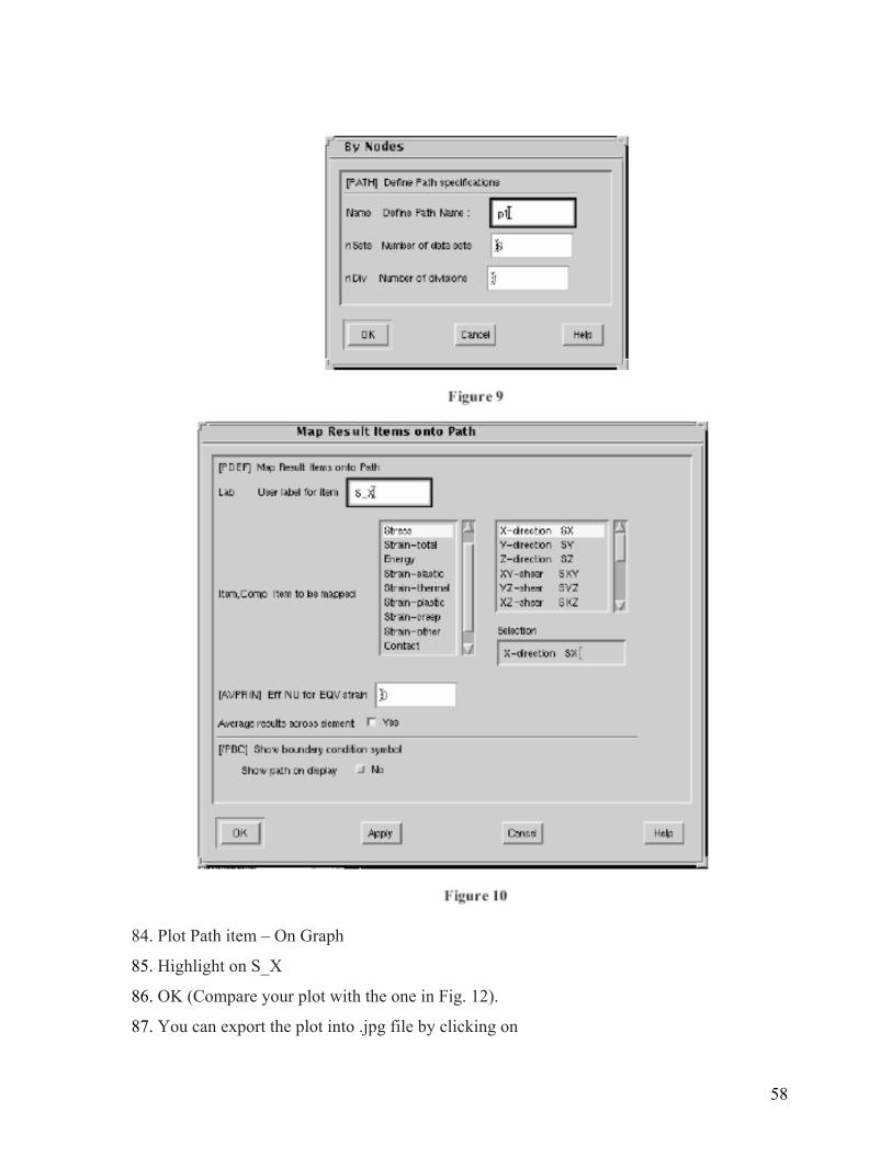
58

84. Plot Path item – On Graph

85. Highlight on S_X

86. OK (Compare your plot with the one in Fig. 12).

87. You can export the plot into .jpg file by clicking on

59

88. PlotCtrls – Hard Copy (check -.graphics window, color, JPEG, landscape, save to)

(you can specify full path name for saving hard copy i.e.,

/home/me_h2/yourid/mech3130/ansys/2dstress/tutorial/graph.jpg )

89. List Path item

90. Highlight on S_X

91. OK

92. Save this ASCII file ( as .txt format) for plotting with other external plotting routines.

60

2D STRESS ANALYSIS & SCF - Exercise

1.

A photo elastic sheet of 1.5 inch width 6 inch length and 0.115 in thickness has a symmetrically

located 0.5 inch diameter circular cut-out. Plot the variation of σx along the line connecting the

top of the hole boundary and the top edge of the plate both from FEA. E=3.2 GPa, υ = 0.34.

Sheet is subjected to a load of 100 psi on the two side boundaries.

2.

A thin sheet of aluminum (AL 6061-T6) is subjected to uniform tension as shown. The sheet

has circular cut-outs as shown in the Figure. Assume that the sheet is 4 inches wide, 18 inches

long, ¼ inch thick, the central cut-out has a diameter of 2 inch, smaller cut-outs have a diameter

of ½ inch and the sheet is subjected to a load of 400 lbs. Your report should include plots of

SCF vs. R/L at (a) the primary hole, (b) the secondary hole. Also, discuss the influence of

eccentricity parameter R/L on the SCF at each location. The various values of L to be used in

the simulations are 3 and 6 inches.

61

Lab # 12

ANSYS™ - CAD IGES INTERFACE AND ANALYSIS - Tutorial

A chair as shown in the figure is subjected to a load of a person sitting on it. Assume that 2/3 of

the person’s load is acting on the seat and the remaining is acting on the back rest of the chair.

Model the given chair in solid edge software and analyze the same in Ansys to find the deformed

shape due to the simultaneous loads.

Assumptions:

1. The weight of the person sitting is 150 pounds.

2. The chair is made up of a material with the following properties

Young’s modulus = 1.34e6 and, Poisson’s ratio = 0.4

3. The rear two legs of the chair have all degrees of freedom constrained and the other two legs

have the z axis displacement constrained.

62

Procedure to solve the problem

Solid edge modeling

1. Open Solid edge software.

2. Click on new model.

3. Click on the sketch icon and select the plane to sketch

Fig 1

4. Click on the line icon(Fig 1)

5. Click at points on the sketching plane to draw lines.

6. Change the dimensions and orientation of the lines to suit.

7. Sketch the cross section of the body of the chair(except the legs)(fig 3)

8. Click on Return.

63

Fig 2

Fig 3

64

9. Select the Sketch 1 from the tree outline and click on the protrude icon.

10. Choose to select from sketch from the drop down menu

11. Now click on the icon.

12. Specify the depth of the protrusion.

13. Click on Return

Fig 4

65

Fig 5&6

66

14. Using the sketch and extrude command in the same way complete the modeling of the

legs of the chair (Fig 5&6, arrive at Fig 7).

15. Select the sides of the chair where you had previously chosen planes.

16. Finish the model and save it in .igs format using the ‘Save as’ command.

Fig 7

Analysis using ANSYS:

Import model to ANSYS:

1. Open the ANSYS window.

2. Click on file – import – IGES

3. Check yes for all options and click OK

4. Click browse on the next window and select the igs file you had saved using Solid Edge

67

Fig 8&9

68

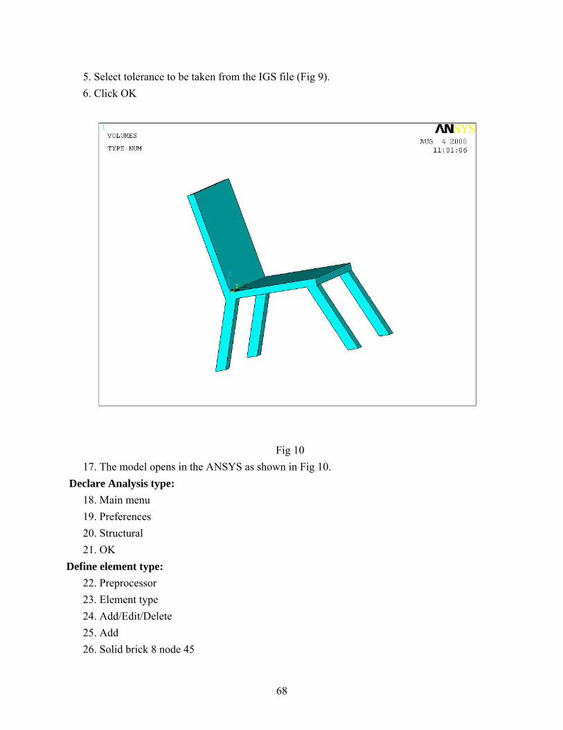
5. Select tolerance to be taken from the IGS file (Fig 9).

6. Click OK

Fig 10

17. The model opens in the ANSYS as shown in Fig 10.

Declare Analysis type:

18. Main menu

19. Preferences

20. Structural

21. OK

Define element type:

22. Preprocessor

23. Element type

24. Add/Edit/Delete

25. Add

26. Solid brick 8 node 45

69

27. OK

28. Close


29. Preprocessor

30. Material Props

31. Material model (double click)

Structural

Linear

Elastic

Isotropic

EX 1.34e6 (this is Young’s modulus)

PRXY 0.4 (this is Poisson’s Ratio)

OK

Close the window

Create nodes and Elements (Meshing of Rod elements):

32. The volume is not in a topology to be divided into perfect 4-6 sided elements.

33. It has to be divided into Volumes suitable for meshing

34. Type the following commands in the ANSYS command prompt.

35. wpstyl,defa

36. vsbw,all

37. wpoffs,0,0,-1

38. vsbw,all

39. Now the chair is divided into 6 volumes viz, four legs, one base and one back part (Fig 11).

40. Click on pre-processor

Meshing

Mesh

Volume

Mapped

4-6 sided

41. Select the four legs and the back of the chair.

42. The base of the chair is still not in the topology for meshing.

70

43. Click on pre-processor

Meshing

Mesh

Volume sweep

Sweep

44. Select the base of the chair.

Fig 11

71

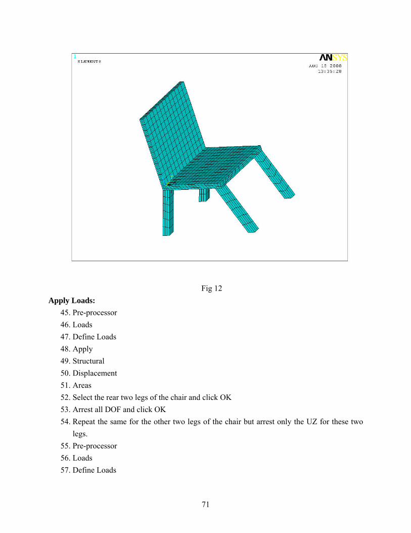
Fig 12

Apply Loads:

45. Pre-processor

46. Loads

47. Define Loads

48. Apply

49. Structural

50. Displacement

51. Areas

52. Select the rear two legs of the chair and click OK

53. Arrest all DOF and click OK

54. Repeat the same for the other two legs of the chair but arrest only the UZ for these two

legs.

55. Pre-processor

56. Loads

57. Define Loads

72

58. Apply

59. Structural

60. Pressure

61. Areas

62. Select the area of the seat of the chair

63. Enter the value of pressure load.(calculate the pressure load from the data given)

64. Repeat the same for the back rest part of the chair

Solve the problem:

65. Solution

66. Solve

67. Current LS

68. OK

Post processing the results:

69. General post processor

70. Plot results

71. Deformed shape(Fig 13)

72. Def + undeformed

73. OK

Fig 13

73

ANSYS™ - CAD IGES INTERFACE AND ANALYSIS - Exercise

1. Model the chair with the following changes to the Dimensions

The thickness of the legs is reduced to1.2” from 1.5 inches.

The thickness of the other portions of the chair is reduced to 0.8” instead of 1”.

The legs and the seat are now perpendicular to each other.(90o instead of the 110o and

114o)

2. Assume the material to be Aluminum (E=10e6 psi and Poisson’s ratio = 0.3).The weight

of the person sitting on the chair is now 200 pounds. The other conditions remain the

same as in the tutorial.

3. Report the deformed shapes for both the cases.(tutorial and exercise).

4. From your analysis which do you think is the safer chair of the two cases and why?

MECH 3130: Mechanics of Materials Fall 2015 Laboratory ...htippur/mech7300-16/MECH3130-Vol2 - Fall...

Documents

Transcript of MECH 3130: Mechanics of Materials Fall 2015 Laboratory ...htippur/mech7300-16/MECH3130-Vol2 - Fall...