Measuring tissue variations in the human brain using ...
172
Measuring tissue variations in the human brain using quantitative MRI Surabhi Sood A thesis submitted for the degree of Doctor of Philosophy at The University of Queensland in 2018 Queensland Brain Institute & Centre for Advance Imaging
Transcript of Measuring tissue variations in the human brain using ...

Measuring tissue variations in the human brain using quantitative MRI
Surabhi Sood
A thesis submitted for the degree of Doctor of Philosophy at
The University of Queensland in 2018
Queensland Brain Institute & Centre for Advance Imaging

1
Abstract
For decades, magnetic resonance imaging has shown overwhelming utility in the
diagnosis and monitoring of diseases and disorders. In the human brain, it has been used
to assess changes in brain structure and function in both healthy and unhealthy individuals
and across patient cohorts. Contrast in structural images has been derived from proton
density, and relaxation based (T1, T2 and T2*) processes. Moreover, methods such as
perfusion, diffusion and functional imaging have provided complementary information in
the assessment of neurodegenerative diseases and disorder affecting the central nervous
system. With the availability of ultra-high field imaging, new contrast mechanisms are able
to provide additional information that can be derived from magnetic resonance imaging
data. In particular, not only the magnitude of the magnetic resonance imaging signal
contains important information, but also the signal phase, which is highly sensitive to
changes in magnetic properties of tissues and the effect scales with field strength. In
quantitative susceptibility mapping, a method that is still under development, phase
images allow the derivation of susceptibility maps. These maps can contain vital
information about iron deposition, calcification, microbleeds, and changes in tissue
microstructure.
The overall aim of my research was to improve the utility of the approach by analysing
quantitative susceptibility maps derived from multi-echo gradient recalled echo magnetic
resonance imaging signals. I made three significant advances. First, I used quantitative
susceptibility mapping at an ultra-high field and studied the temporal trends in magnetic
susceptibility using signal compartmentalisation. I found the trends in magnetic
susceptibility as a function of echo time are influenced by tissue microstructure
differences. This information is potentially useful in identifying changes in tissue
microstructure in the human brain.
Second, I investigated how changes in temporal magnetic susceptibility change as a
function of the magnetic field strength of the MRI scanner. I found the processing pipeline
and field strength to affect signal compartmentalisation, however consistent results can be
generated provided a distinct processing pipeline is used.
Third, I studied how signal compartments could be used to parcellate cortical regions in
the human brain. I examined the use of single and multiple orientation quantitative
susceptibility mapping methods. I found cortical regions can potentially be parcellated
using signal compartmentalisation of the multiple echo gradient recalled echo MRI signal.
My work may lead to full parcellation of the human brain and help explore how parcellated

2
brain regions play a role in brain development and how they change with brain diseases
and disorders.
3
Declaration by author
This thesis is composed of my original work, and contains no material previously published
or written by another person except where due reference has been made in the text. I
have clearly stated the contribution by others to jointly-authored works that I have included
in my thesis.
I have clearly stated the contribution of others to my thesis as a whole, including
statistical assistance, survey design, data analysis, significant technical procedures,
professional editorial advice, financial support and any other original research work used
or reported in my thesis. The content of my thesis is the result of work I have carried out
since the commencement of my higher degree by research candidature and does not
include a substantial part of work that has been submitted to qualify for the award of any
other degree or diploma in any university or other tertiary institution. I have clearly stated
which parts of my thesis, if any, have been submitted to qualify for another award.
I acknowledge that an electronic copy of my thesis must be lodged with the University
Library and, subject to the policy and procedures of The University of Queensland, the
thesis be made available for research and study in accordance with the Copyright Act
1968 unless a period of embargo has been approved by the Dean of the Graduate School.
I acknowledge that copyright of all material contained in my thesis resides with the
copyright holder(s) of that material. Where appropriate I have obtained copyright
permission from the copyright holder to reproduce material in this thesis and have sought
permission from co-authors for any jointly authored works included in the thesis.

4
Publications during candidature
Surabhi Sood, Javier Urriola, David Reutens, Kieran O’Brien, Steffen Bollmann, Markus
Barth, Viktor Vegh, “Echo time dependent quantitative susceptibility mapping contains
information on tissue properties”. Magnetic Resonance in Medicine, 77.5 (2017): 1946-
1958.
Conference abstracts
Surabhi Sood, David Reutens, Shrinath Kadamangudi, Markus Barth and Viktor Vegh,
“Echo time dependence in temporal frequency shift curves at 3T and 7T”. International
society for Magnetic Resonance in Medicine, Paris, 2018.
Qiang Yu, David Reutens, Javier Urriola, Surabhi Sood and Viktor Vegh, “MRI
approaches to map focal cortical dysplasia in focal epilepsy using anomalous diffusion and
magnetic susceptibility”. International society for Magnetic Resonance in Medicine, Paris,
2018.
Surabhi Sood, David Reutens, Steffen Bollmann, Kieran O’Brien, Markus Barth and Viktor
Vegh, “Temporal quantitative susceptibility mapping of cortical regions”. Organization for
Human Brain Mapping, Vancouver, 2017.
Shrinath Kadamangudi, Surabhi Sood, David Reutens and Viktor Vegh,
“Discrete frequency shift signatures explain GRE-MRI signal compartments”. International
society for Magnetic Resonance in Medicine, Honolulu, 2017.
Viktor Vegh, Surabhi Sood, Shrinath Kadamangudi, Kiran Thapaliya, Markus Barth and
David Reutens, “Where can multi-echo gradient recalled MRI signal compartments take
us”. Australian and New Zealand Society for Magnetic Resonance, New South Wales,
2017.
Surabhi Sood, Javier Urriola, David Reutens, Steffen Bollmann, Kieran O’Brien, Markus
Barth and Viktor Vegh, “Echo time based dependence in quantitative susceptibility
mapping”. International society for Magnetic Resonance in Medicine, Singapore, 2016.
Surabhi Sood, Javier Urriola, Steffen Bollmann, Markus Barth, Kieran O’Brien, David
Reutens and Viktor Vegh, “Contribution of cortical layer cytoarchitecture to quantitative
susceptibility mapping”. Organization for Human Brain Mapping, Geneva, 2016.
5
Symposium
Surabhi Sood, David Reutens, Kieran O’ Brien, Markus Barth and Viktor Vegh, “Echo time
based influences on quantitative susceptibility mapping”. Princess Alexandra Hospital
Health Symposium, Brisbane, 2017.
Surabhi Sood, Markus Barth, Kieran O’Brien, David Reutens and Viktor Vegh, “Exploring
echo time dependence in quantitative susceptibility mapping”. The Centre for Advanced
Imaging 3rd Annual Symposium co-hosted with Singapore Bioimaging Consortium,
Brisbane, 2016.
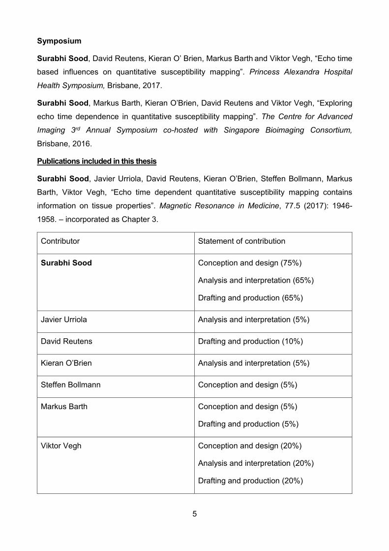
Publications included in this thesis
Surabhi Sood, Javier Urriola, David Reutens, Kieran O’Brien, Steffen Bollmann, Markus
Barth, Viktor Vegh, “Echo time dependent quantitative susceptibility mapping contains
information on tissue properties”. Magnetic Resonance in Medicine, 77.5 (2017): 1946-
1958. – incorporated as Chapter 3.
Contributor Statement of contribution
Surabhi Sood Conception and design (75%)
Analysis and interpretation (65%)
Drafting and production (65%)
Javier Urriola Analysis and interpretation (5%)
David Reutens Drafting and production (10%)
Kieran O’Brien Analysis and interpretation (5%)
Steffen Bollmann Conception and design (5%)
Markus Barth Conception and design (5%)
Drafting and production (5%)
Viktor Vegh Conception and design (20%)
Analysis and interpretation (20%)
Drafting and production (20%)

6
Manuscripts included in this thesis
Surabhi Sood, David Reutens, Shrinath Kadamangudi, Markus Barth and Viktor Vegh,
“Evaluation of 3T and 7T gradient recalled echo MRI signal compartment frequency shifts”.
Scientific Reports, (under revision).
Contributor Statement of contribution
Surabhi Sood Conception and design (75%)
Analysis and interpretation (80%)
Drafting and production (65%)
David Reutens Drafting and production (10%)
Shrinath Kadamangudi Conception and design (10%)
Markus Barth Drafting and production (5%)
Viktor Vegh Conception and design (20%)
Analysis and interpretation (20%)
Drafting and production (20%)
Surabhi Sood, David Reutens, Markus Barth and Viktor Vegh, “Evaluation of multi-echo
gradient recalled echo magnetic resonance imaging towards parcellating the human
cerebral cortex”. Neuroimage, (submitted)
Contributor Statement of contribution
Surabhi Sood Conception and design (80%)
Analysis and interpretation (80%)
Drafting and production (65%)
David Reutens Drafting and production (10%)
Markus Barth Drafting and production (5%)
Viktor Vegh Conception and design (20%)

7
Analysis and interpretation (20%)
Drafting and production (20%)
Conference abstracts
Surabhi Sood, David Reutens, Shrinath Kadamangudi, Markus Barth and Viktor Vegh,
“Echo time dependence in temporal frequency shift curves at 3T and 7T”. International
society for Magnetic Resonance in Medicine, Paris, 2018.
Contributor Statement of contribution
Surabhi Sood Conception and design (85%)
Analysis and interpretation (80%)
Drafting and production (75%)
Shrinath Kadamangudi Analysis and interpretation (5%)
David Reutens Drafting and production (5%)
Markus Barth Drafting and production (5%)
Viktor Vegh Conception and design (15%)
Analysis and interpretation (15%)
Drafting and production (15%)
Qiang Yu, David Reutens, Javier Urriola, Surabhi Sood and Viktor Vegh, “MRI
approaches to map focal cortical dysplasia in focal epilepsy using anomalous diffusion and
magnetic susceptibility”. International society for Magnetic Resonance in Medicine, Paris,
2018.
Contributor Statement of contribution
Surabhi Sood Analysis and interpretation (50%)

8
Qiang Yu Conception and design (65%)
Analysis and interpretation (35%)
Drafting and production (80%)
David Reutens Drafting and production (5%)
Javier Urriola Conception and design (20%)
Viktor Vegh Conception and design (15%)
Analysis and interpretation (15%)
Drafting and production (15%)
Surabhi Sood, David Reutens, Steffen Bollmann, Kieran O’Brien, Markus Barth and Viktor
Vegh, “Temporal quantitative susceptibility mapping of cortical regions”. Organization for
Human Brain Mapping, Vancouver, 2017.
Contributor Statement of contribution
Surabhi Sood Conception and design (70%)
Analysis and interpretation (80%)
Drafting and production (70%)
David Reutens Drafting and production (5%)
Steffen Bollmann Conception and design (5%)
Drafting and production (5%)
Kieran O’Brien Conception and design (5%)
Markus Barth Conception and design (5%)
Drafting and production (5%)
Viktor Vegh Conception and design (15%)
9
Analysis and interpretation (20%)
Drafting and production (15%)
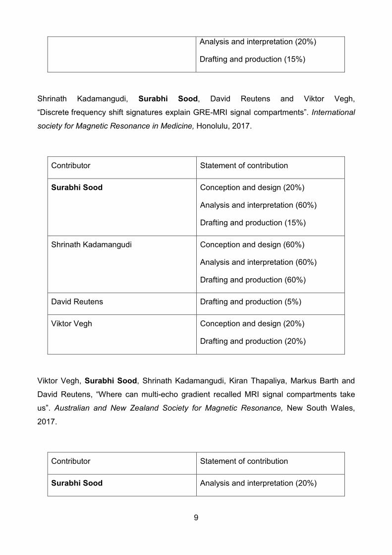
Shrinath Kadamangudi, Surabhi Sood, David Reutens and Viktor Vegh,
“Discrete frequency shift signatures explain GRE-MRI signal compartments”. International
society for Magnetic Resonance in Medicine, Honolulu, 2017.
Contributor Statement of contribution
Surabhi Sood Conception and design (20%)
Analysis and interpretation (60%)
Drafting and production (15%)
Shrinath Kadamangudi Conception and design (60%)
Analysis and interpretation (60%)
Drafting and production (60%)
David Reutens Drafting and production (5%)
Viktor Vegh Conception and design (20%)
Drafting and production (20%)
Viktor Vegh, Surabhi Sood, Shrinath Kadamangudi, Kiran Thapaliya, Markus Barth and
David Reutens, “Where can multi-echo gradient recalled MRI signal compartments take
us”. Australian and New Zealand Society for Magnetic Resonance, New South Wales,
2017.
Contributor Statement of contribution
Surabhi Sood Analysis and interpretation (20%)

10
Drafting and production (10%)
Viktor Vegh Conception and design (75%)
Analysis and interpretation (60%)
Drafting and production (60%)
Shrinath Kadamangudi Conception and design (5%)
Analysis and interpretation (10%)
Drafting and production (15%)
Kiran Thapaliya Analysis and interpretation (10%)
Drafting and production (5%)
Markus Barth Drafting and production (5%)
David Reutens Drafting and production (5%)
Surabhi Sood, Javier Urriola, David Reutens, Steffen Bollmann, Kieran O’Brien, Markus
Barth and Viktor Vegh, “Echo time based dependence in quantitative susceptibility
mapping”. International society for Magnetic Resonance in Medicine, Singapore, 2016.
Contributor Statement of contribution
Surabhi Sood Conception and design (65%)
Analysis and interpretation (60%)
Drafting and production (55%)
Javier Urriola Analysis and interpretation (15%)
David Reutens Drafting and production (10%)
Kieran O’Brien Conception and design (5%)
Steffen Bollmann Conception and design (5%)

11
Analysis and interpretation (5%)
Drafting and production (5%)
Markus Barth Conception and design (5%)
Drafting and production (10%)
Viktor Vegh Conception and design (20%)
Analysis and interpretation (20%)
Drafting and production (20%)
Surabhi Sood, Javier Urriola, Steffen Bollmann, Markus Barth, Kieran O’Brien, David
Reutens and Viktor Vegh, “Contribution of cortical layer cytoarchitecture to quantitative
susceptibility mapping”. Organization for Human Brain Mapping, Geneva, 2016. –
incorporated as Chapter 4.
Contributor Statement of contribution
Surabhi Sood Conception and design (60%)
Analysis and interpretation (60%)
Drafting and production (55%)
Javier Urriola Analysis and interpretation (15%)
Steffen Bollmann Conception and design (5%)
Analysis and interpretation (5%)
Drafting and production (5%)
Markus Barth Conception and design (5%)
Drafting and production (10%)
Kieran O’Brien Conception and design (5%)
David Reutens Drafting and production (10%)

12
Viktor Vegh Conception and design (20%)
Analysis and interpretation (20%)
Drafting and production (20%)
Symposium
Surabhi Sood, David Reutens, Kieran O’ Brien, Markus Barth and Viktor Vegh, “Echo time
based influences on quantitative susceptibility mapping”. Princess Alexandra Hospital
Health Symposium, Brisbane, 2017.
Contributor Statement of contribution
Surabhi Sood Conception and design (70%)
Analysis and interpretation (80%)
Drafting and production (60%)
David Reutens Drafting and production (10%)
Kieran O’Brien Conception and design (5%)
Markus Barth Conception and design (5%)
Drafting and production (10%)
Viktor Vegh Conception and design (20%)
Analysis and interpretation (20%)
Drafting and production (20%)
Surabhi Sood, Markus Barth, Kieran O’Brien, David Reutens and Viktor Vegh, “Exploring
echo time dependence in quantitative susceptibility mapping”. The Centre for Advanced
Imaging 3rd Annual Symposium co-hosted with Singapore Bioimaging Consortium,
Brisbane, 2016.

13
Contributor Statement of contribution
Surabhi Sood Conception and design (75%)
Analysis and interpretation (65%)
Drafting and production (70%)
Marcus Barth Analysis and interpretation (15%)
Kieran O’Brien Conception and design (5%)
David Reutens Drafting and production (10%)
Viktor Vegh Conception and design (20%)
Analysis and interpretation (20%)
Drafting and production (20%)
14
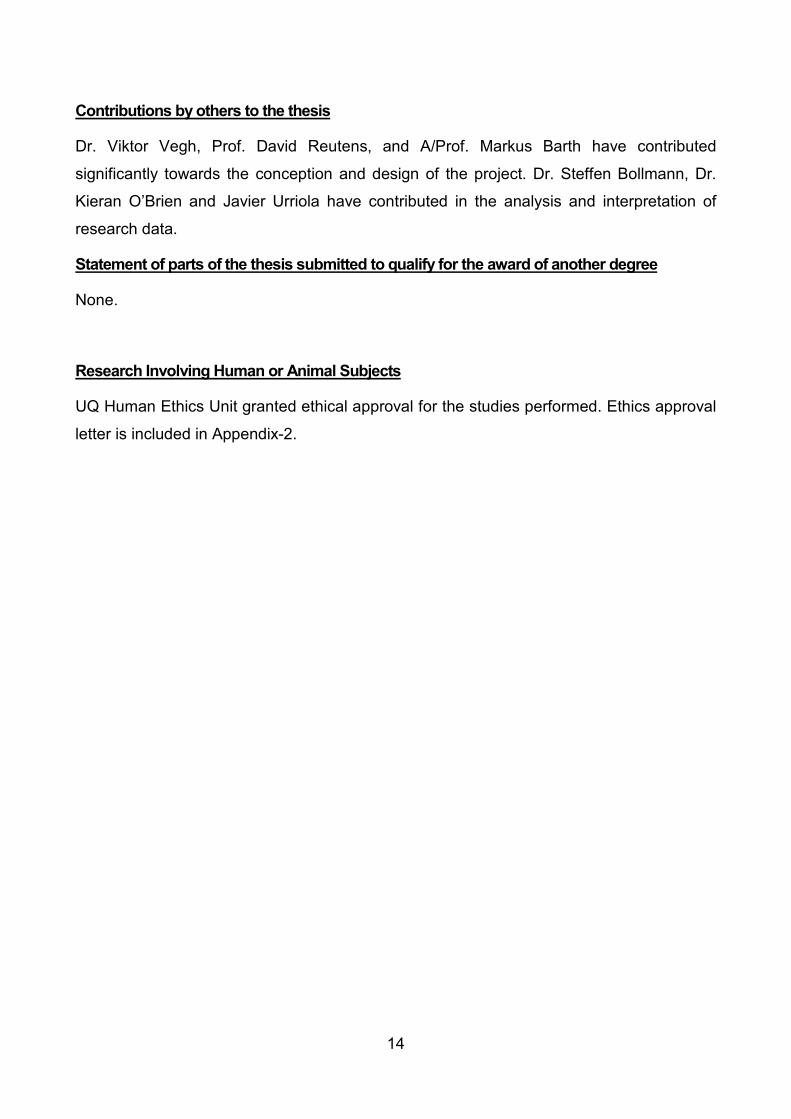
Contributions by others to the thesis
Dr. Viktor Vegh, Prof. David Reutens, and A/Prof. Markus Barth have contributed
significantly towards the conception and design of the project. Dr. Steffen Bollmann, Dr.
Kieran O’Brien and Javier Urriola have contributed in the analysis and interpretation of
research data.
Statement of parts of the thesis submitted to qualify for the award of another degree
None.
Research Involving Human or Animal Subjects
UQ Human Ethics Unit granted ethical approval for the studies performed. Ethics approval
letter is included in Appendix-2.

15
Acknowledgements
I would like to express my gratitude to Dr. Viktor Vegh whose knowledge, support and
encouragement made this dissertation possible. I would also like to thank Prof. David
Reutens and A/Prof. Markus Barth for their mentorship throughout my PhD.
I am grateful to Dr. Steffen Bollmann, Dr. Kieran O’Brien and Javier Urriola for their
technical guidance. I also appreciate Aiman Al-Najjar and Nicole Atcheson for their
contribution in data collection. I recognise the suggestions from my assessors: Dr. Gary
Cowin and Dr. Nyoman Kurniawan. I deeply acknowledge the support of my family and
friends during my PhD journey.
Viktor Vegh and David Reutens acknowledge the National Health and Medical
Research Council (NHMRC Project Grant – APP1104933) for funding our research.
Markus Barth acknowledges funding received for his Australian Research Council Future
Fellowship (FT140100865).

16
Financial support
This research was supported by an Australian Government Research Training Program
Scholarship.

17
Keywords
Ultra-high field MRI, phase imaging, quantitative susceptibility mapping, echo time
dependence, phase unwrapping, orientation in phase imaging.
Australian and New Zealand Standard Research Classifications (ANZSRC)
ANZSRC code: 110903, Central Nervous System, 60%
ANZSRC code: 029903, Medical Physics, 20%
ANZSRC code: 029901, Biological Physics, 20%
Fields of Research (FoR) Classification
FoR code: 1109, Neurosciences, 60%
FoR code: 0299, Other Physical Sciences, 40%
18
Table of Contents
Abstract ............................................................................................................................... 1
Declaration by author .......................................................................................................... 3
Publications during candidature .......................................................................................... 4
Publications included in this thesis ..................................................................................... 5
Contributions by others to the thesis ................................................................................. 14
Statement of parts of the thesis submitted to qualify for the award of another degree ..... 14
Research Involving Human or Animal Subjects ................................................................ 14
Acknowledgements ........................................................................................................... 15
Financial support .............................................................................................................. 16
Keywords .......................................................................................................................... 17
Australian and New Zealand Standard Research Classifications (ANZSRC) ................... 17
Fields of Research (FoR) Classification ............................................................................ 17
Table of Contents ............................................................................................................. 18
List of Figures ................................................................................................................... 22
List of Tables .................................................................................................................... 28
List of Abbreviations .......................................................................................................... 30
Chapter 1 Introduction .................................................................................................... 32
1.1 Magnetic resonance imaging ................................................................................ 33
1.2 Susceptibility Weighted Imaging ........................................................................... 35
1.3 Quantitative Susceptibility Mapping ...................................................................... 36
1.4 QSM at ultra-high field .......................................................................................... 39
1.5 QSM processing ................................................................................................... 40
1.5.1 Phase processing ........................................................................................... 41
1.5.2 Brain masks ................................................................................................... 45
1.5.3 Dipole inversion .............................................................................................. 46
1.6 Compartment modelling using multiple echo time GRE-MRI phase data ............ 48

19
1.7 Utility of ultra-high field MRI .................................................................................. 51
1.8 GRE in cerebral cortex ......................................................................................... 52
1.9 Applications of QSM ............................................................................................. 53
1.9.1 Quantification of iron deposits ........................................................................ 53
1.9.2 Traumatic brain injury ..................................................................................... 55
1.9.3 Multiple Sclerosis ........................................................................................... 56
1.9.4 Brain Tumour ................................................................................................. 57
1.10 QSM reconstruction challenge .......................................................................... 58
Chapter 2 Research aims and hypothesis ...................................................................... 60
Aim 1: Echo-time dependent quantitative susceptibility mapping contains information
on tissue properties - Chapter 3 ................................................................................. 61
Aim 2: Contribution of cortical layer cytoarchitecture to quantitative susceptibility
mapping - Chapter 4 ................................................................................................... 61
Aim 3: Field strength influences on gradient recalled echo MRI signal compartment
frequency shifts - Chapter 5 ........................................................................................ 62
Aim 4: Evaluation of multi-echo QSM in the brain cortex using ultra-high field -
Chapter 6 .................................................................................................................... 62
Chapter 3 Echo-time dependent quantitative susceptibility mapping contains information
on tissue properties ........................................................................................................... 63
3.1 Abstract ................................................................................................................ 63
3.2 Introduction ........................................................................................................... 64
3.3 Methods ................................................................................................................ 66
3.3.1 Data acquisition .............................................................................................. 66
3.3.2 Data reconstruction pipeline ........................................................................... 67
3.3.3 Manual region-of-interest selection ................................................................ 67
3.3.4 Mapping of susceptibility across echo time .................................................... 68
3.3.5 Multi-compartment contributions to susceptibility ........................................... 68
3.4 Results .................................................................................................................. 71

20
3.4.1 tQSM curves .................................................................................................. 71
3.4.2 Parameterisation of signal compartments ...................................................... 72
3.5 Discussion ............................................................................................................ 77
3.5.1 Considerations for QSM studies ..................................................................... 80
3.5.2 Methodological considerations ....................................................................... 81
3.6 Conclusion ............................................................................................................ 82
Chapter 4 Contribution of cortical layer cytoarchitecture to quantitative susceptibility
mapping 84
4.1 Introduction ........................................................................................................... 84
4.2 Methods ................................................................................................................ 84
4.3 Results .................................................................................................................. 85
4.4 Conclusions .......................................................................................................... 87
Chapter 5 Field strength influences on gradient recalled echo MRI signal
compartment frequency shifts ............................................................................................ 89
5.1 Abstract ................................................................................................................ 89
5.2 Introduction ........................................................................................................... 89
5.3 Methods ................................................................................................................ 91
5.3.1 Data Acquisition ............................................................................................. 91
5.3.2 Data Processing ............................................................................................. 92
5.3.3 Regions-of-interest ......................................................................................... 93
5.3.4 GRE-MRI signal compartment fitting .............................................................. 93
5.4 Results .................................................................................................................. 94
5.4.1 Frequency shifts as a function of echo time ................................................... 94
5.4.2 Signal compartmentalisation .......................................................................... 95
5.5 Discussion .......................................................................................................... 103
5.5.1 Previous findings on echo time dependence ................................................ 103
5.5.2 Signal compartments ................................................................................... 104

21
5.6 Conclusion .......................................................................................................... 105
Chapter 6 Evaluation of multi-echo QSM in the brain cortex using ultra-high field ....... 107
6.1 Abstract .............................................................................................................. 107
6.2 Introduction ......................................................................................................... 107
6.3 Materials and Methods ....................................................................................... 109
6.3.1 MRI data acquisition ..................................................................................... 109
6.3.2 Single orientation susceptibility mapping ..................................................... 110
6.3.3 Multiple orientation susceptibility mapping ................................................... 111
6.3.4 Cortical areas ............................................................................................... 112
6.3.5 GRE-MRI signal compartment fitting ............................................................ 113
6.4 Results ................................................................................................................ 114
6.4.1 Trends in temporal frequency shift curves in cortical regions ....................... 117
6.4.2 Difference measure between temporal frequency shift curves ..................... 118
6.4.3 Test of signal compartment model parameters across cortical regions ........ 120
6.5 Discussion .......................................................................................................... 123
6.5.1 Echo time dependent trends in frequency shift curves ................................. 124
6.5.2 Signal compartment model parameter variations ......................................... 124
6.5.3 Multiple versus single orientation data ......................................................... 125
6.5.4 Methodological considerations ..................................................................... 126
6.6 Conclusion .......................................................................................................... 127
Chapter 7 Conclusions and Future directions ............................................................... 128
Reference ....................................................................................................................... 128
Appendices ..................................................................................................................... 143

22
List of Figures
Figure 1.1 Flowcharts of processing steps of SWI (a) and QSM (b). (a) SWI combines both
the magnitude and a filtered phase map in a multiplicative relationship to enhance image
contrast. Minimum intensity projection (MIP) is commonly applied to highlight the veins.
SWI flowchart adapted from Reichenbach et al. (b) There are two major steps involved in
QSM: filtering background phase and solving an inverse problem. ................................... 36
Figure 1.2 Susceptibility source and MR signal phase. ..................................................... 38
Figure 1.3 2D Pulse sequence diagram for gradient recalled echo. RF is (the) radio
frequency pulse, SLICE is (the) slice selection gradient, PHASE is (the) phase encoding
gradient, READOUT is the readout gradient, ADC is the analog-to-digital converter, and
SIGNAL is the signal acquired. The amplitude of the phase encoding gradient is changed
to obtain different k-space lines. ........................................................................................ 39
Figure 1.4 Schematic illustration of the general QSM pipeline used to obtain susceptibility
maps from raw phase images acquired using gradient recalled echo magnetic resonance
imaging sequences. ........................................................................................................... 41
Figure 1.5 Comparison of unwrapped phase images by Catalytic multiecho phase
unwrapping Scheme (CAMPUS), phase unwrapping (PhUN), and the branch cut
algorithms for four normal volunteers. To avoid the cusp artefact observed in the scanner-
combined phase images, these phase images were derived from complex division(s) of
echo 10 by echo 1 to give an effective echo time of 23.67ms. White arrow in (c-4) points to
a few voxels incorrectly unwrapped by CAMPUS due to the violation of slow flow
assumption. The black arrows in row (d) and (e) point to areas where PhUN and the
branch cut algorithms failed to unwrap. Note that the phase images were scaled to the full
gray scale range for better visualization. Source:(32) ........................................................ 43
Figure 1.6 Comparison of the background-removed phase and magnetic susceptibility
obtained using different phase processing methods. (A, B) Tissue phase images obtained
using HARPERELLA [HARmonic (background) PhasE REmovaL using the LAplacian
operator]. (C, D) Tissue phase images obtained using path-based phase unwrapping and
V-SHARP (sophisticated harmonic artefact reduction for phase data with varying spherical
kernel sizes). (E, F) Tissue phase images obtained using path-based phase unwrapping
and PDF (projection onto dipole fields). (G, H) Phase difference between the results
obtained with HARPERELLA and path-based phase unwrapping plus PDF. (I, J)
Susceptibility maps derived from HARPERELLA-processed phase images. (K, L)

23
Susceptibility maps derived from phase images obtained using path-based phase
unwrapping and V-SHARP. (M, N) Susceptibility maps derived from phase images
obtained using path-based phase unwrapping and PDF. (O, P) Difference between the
susceptibility maps obtained with HARPERELLA and path-based phase unwrapping plus
PDF. Source:(30) ............................................................................................................... 45
Figure 1.7 Susceptibility map with streaking artefacts (a) and without streaking artefacts
(b). ..................................................................................................................................... 48
Figure 1.8 (a) The object is scanned at the first position. Then the object is rotated around
the x-axis. (b) The scan is repeated at the second orientation. The rotation-scanning
process repeats until the required number of rotations is reached. Subsequent rotations
are not shown here. (c) The dipole response kernel function in the Fourier domain (fixed
with respect to the object) has zeros located on a pair of cone surfaces (the green pair for
the first sampling and the blue pair for the second sampling). The presence of these zeros
makes the inversion extremely susceptible to noise and they need to be avoided when
possible. Sampling from two orientations is insufficient because these two pairs of cone
surfaces will still intercept, resulting in lines of common zeros. Sampling from an
appropriate third angle can eliminate all the common zeros in the dipole kernels except the
origin, which only defines a constant offset but does not change the relative susceptibility
difference between tissues in the image. Source:(64) ....................................................... 48
Figure 1.9 Correlation of bulk magnetic susceptibility with measured iron concentration.
The line represents the regression of all data points and the dotted lines indicate the 95%
confidence intervals. Source:(53) ...................................................................................... 54
Figure 1.10 Mean ± SEM of average susceptibility in ppm computed by the two methods
(ℓ1-regularized QSM, top; ℓ2-regularized QSM, bottom) for each ROI in the young and
elderly groups. Source: (102) and LEM means standard error from the mean. ................. 55
Figure 1.11 Susceptibility map of a sample severe traumatic brain injury case. Each image
represents a slab 8 mm thick after maximal intensity projection across four slices, each
2 mm thick. Left and right images show different levels of the same brain. Cerebral
microbleeds (solid arrows) demonstrate much brighter signal(s) than surrounding veins
(dashed arrows) and brain tissue. Source:(104) ................................................................ 56
Figure 1.12 Representative R2* maps (top row) and quantitative susceptibility maps
(bottom row) of two 29-year-old individuals, a healthy control subject and an MS patient.
Note increased (more paramagnetic) susceptibility in the basal ganglia in the MS patient.

24
Differences are most evident in the putamen (arrow, 0.049 vs 0.092 ppm). Image window
settings were identical: R2* mapping, from 0 (black) to 40 sec−1(white); QSM, from −0.1
(black) to 0.25 ppm (white). Source:(105) .......................................................................... 57
Figure 1.13 Images of a 42 year old man with a glioblastoma in the right occipital lobe
(patient B1), who was treated with 12 cycles of bevacizumab after completion of
radiochemotherapy(,) are presented in the upper part (a–e). The lower part (f–j) reveals
images of a 46 year old man with a glioblastoma in the frontal lobe (patient B2), who was
treated with 5 cycles of bevacizumab. T1-weighted images before (a,f) and after contrast
agent administration (b,g), FLAIR images (c,h), SW images (d,i) and susceptibility maps
(e,j) are presented for each patient. The patient in the upper part represents SBS that only
correlate(s) with hyperintense areas on the susceptibility maps (arrow heads), whereas the
patient in the lower part reveals additional calcifications indicated by hypointense
correlates of SBS on susceptibility maps (arrows). Source:(106) ...................................... 58
Figure 3.1 Illustration of the pipeline used to compute quantitative susceptibility maps.
Individual channel data were processed using STI Suite and combined into a single image
at the very end. .................................................................................................................. 66
Figure 3.2 Illustration of the location of the ten human brain regions-of-interest used to
assess changes in magnetic susceptibility. ........................................................................ 68
Figure 3.3 tQSM results for (a) caudate, (b) internal capsule, (c) red nucleus and (d)
corpus callosum. Individual plots show the response for each participant (thin solid lines)
along with the group mean (thick solid line) and standard deviation (dashed lines). We
found a trend in susceptibility values with echo time, and the trend varies with (the) region
selected. ............................................................................................................................ 72
Figure 3.4 tQSM results for (a) thalamus, (b) pallidum, (c) substantia nigra, (d) putamen,
(e) fornix and (f) insula. Individual plots show the response for each participant (thin solid
lines) along with the group mean (thick solid line) and standard deviation (dashed lines).
We found a trend in susceptibility values with echo time, and the trend varies with (the)
region selected. ................................................................................................................. 74
Figure 3.5 Shown are tQSM results for sub-regions of the (a) substantia nigra (compact
and reticular), (b) pallidum (internal globus pallidus and external globus pallidus), and (c)
insula (anterior and posterior insula). These regions are known to have different cell
densities and cytoarchitectures, and the susceptibility curve depicts a different pattern for
each case. ......................................................................................................................... 75

25
Figure 3.6 Standard deviation of the mapped magnetic susceptibility within regions across
the ten brain regions plotted over echo time: (a) fornix, (b) caudate, (c) putamen and (d)
internal capsule. Solid line is the mean magnitude signal and dashed lines represent one
standard deviation from the mean. .................................................................................... 77
Figure 3.7 Standard deviation of the mapped magnetic susceptibility within regions across
the ten brain regions plotted over echo time: (a) corpus callosum, (b) red nucleus, (c)
thalamus, (d) insula, (e) pallidum and (f) substantia nigra. (The) Solid line is the mean
magnitude signal and (the) dashed lines represent one standard deviation from the mean.
........................................................................................................................................... 78
Figure 4.1 The primary visual cortex slab: (I) slab orientation, (II) cross section of the slab,
(IIa) zoomed in section of the primary visual cortex. The coloured lines show the voxels
selected across the cortex and the white arrow identifies the line of gennari, and (IIb) (the)
blue colour shows voxels selected along the line of gennari, (while the) red and green
colours show the voxels above and below the line of gennari. Data were averaged along
the red, blue and green lines after the application of the QSM pipeline. ............................ 85
Figure 4.2 The slab cutting across the premotor and primary motor cortices: (I) slab
orientation, (II) cross section of the slab, (IIa) zoomed in section showing coloured lines
across selected voxels in the premotor cortex, and (IIb) zoomed in section showing
coloured lines across selected voxels in the primary motor cortex. Data were averaged on
either side of the top of the cortex (i.e. averaged corresponding locations of the magenta,
yellow and black lines, and averaged corresponding locations of the blue, green, red and
cyan lines). ......................................................................................................................... 86
Figure 4.3 QSM plots of lines selected in the primary visual cortex, corresponding to
Figure 4.1(IIa). A noticeable shift in the curves can be appreciated with a change in
location. ............................................................................................................................. 87
Figure 4.4 Graphs showing plots from the (I, IV) primary visual cortex (granular), and (II, V)
premotor and (III, VI) primary motor cortices (both agranular). In (I-III) each line
corresponds to a different projection perpendicular to the cortex. In (IV-VI) voxel locations
for each line are assessed. Fine lines represent individual measurements and the thick
black line represents the mean of individual measurements computed at each echo time
point. .................................................................................................................................. 88

26
Figure 5.1 Illustration of the brain regions-of-interest used in this study for comparing
temporal frequency shift curves. These are also the regions for which signal
compartmentalisation was performed. ............................................................................... 93
Figure 5.2 Frequency shifts as a function of echo point in the six brain regions obtained
using the Laplacian reconstruction pipeline. Solid lines are the averaged values obtained
for the brain region based on all participants, and the standard deviation of values is
shown using the corresponding colour shaded region corresponds to inter-participant
variability. ........................................................................................................................... 98
Figure 5.3 Frequency shift values as a function of echo point in the six brain regions
obtained using the path-based reconstruction pipeline. Plot description as per Figure 5.2.
........................................................................................................................................... 99
Figure 6.1 Illustration of the Brodmann areas (i.e. regions-of-interest) and orientations of
the two slabs with respect to the scanner field, B0. In (a) cortical regions BA6, BA4, BAV1
and BAV2 are shown over an inflated brain surface, (b) middle slice of the slab acquired in
the axial orientation covering the primary motor cortex, BA4, and premotor cortex, BA6.
Similarly, in (c) the middle slice of the coronal slab used for data acquisition, covering the
primary visual cortex, BAV1, and secondary visual cortex, BAV2, is shown.................... 112
Figure 6.2 ROIs (premotor cortex BA6, primary motor cortex BA4, primary visual cortex
BAV1, and secondary visual cortex BAV2) shown on different slices in (a) coronal, (b)
axial, and (c) sagittal orientation. ..................................................................................... 113
Figure 6.3 Shown are representative images from the 45th slice of the axial slab in the first
participant. Depicted are echo time dependent (A) magnitude images and (B) tissue phase
images in the axial slab, and similarly (C,D) depict the images from the coronal slab. .... 115
Figure 6.4 Weighted average frequency shift curves and corresponding pooled variances
(both in Hz) as a function of echo number are shown for BA6, BA4, BAV1 and BAV2. Plots
have been generated based on three different thresholds (0.06, 0.12 – default, 0.24) in the
TKD method, and using four head positions (normal1, normal2, backward, forward) with
the single orientation data reconstruction pipeline. .......................................................... 117
Figure 6.5 Plots of the Fréchet distance between frequency shift curves for each of the six
participants (P1-P6). The regions between which the Fréchet distance was calculated is
shown on the horizontal axes. Results are provided for three TKD thresholds (0.06, 0.12 –
default, 0.24) and for three orientations (normal1, backward and forward). Note, normal2
results were consistent with normal1 results. ................................................................... 118

27
Figure 6.6 T2* and frequency shift parameter results obtained using a single (N = 1) signal
compartment model based on the TKD data. Depicted are results for the three different
TKD thresholds (0.06, 0.12 – default, 0.24) for the four regions. Error bars represent one
standard deviation from the mean. Significant differences are summarised in Table 6.1.119
Figure 6.7 Results of two compartment (N = 2) model fitting(s) of single orientation
frequency shift curves for each of the regions. Shown are the volume fractions
corresponding to each compartment, and corresponding T2* and frequency shift parameter
values. Error bars correspond to one standard deviation from the mean; 1 and 2 on the
horizontal axes refer to the two signal compartments. Significant differences have been
summarised in Table 6.2. ................................................................................................. 120
Figure 7.1 A connection map of compartment frequency shifts and volume fractions for all
ROI. The akaike information criterion (AIC) -based centroids identified using cluster
analysis are shown on the frequency axis, and the size of the compartments represented
using different sized circles are presented vertically. Each region has been connected to
their respective compartment frequency shift values. The regions have been arranged in
an order which minimizes the number of overlapping lines, simply to assist with the
visualization of signal compartment volume fractions and their frequency shifts. ............ 129

28
List of Tables
Table 1.1 Examples of SWI and QSM protocoles for the brain. Source: (13) .................... 36
Table 3.1Three compartment model fittings results for the ten brain regions. Adjusted R2
represents the quality of fit, and χ is the symbol for magnetic susceptibility and subscripts
denote the three signal compartments. T2* was calculated for the voxel. Values have been
arranged from largest to smallest compartment contribution. ............................................ 75
Table 3.2 Three compartment model fittings for the sub-segmented regions (SN stand for
substantia nigra and GP stands for globus pallidus). Adjusted R2 represents the quality of
fit, and χ provides the calculated value of the magnetic susceptibility across the three
compartments. T2* was calculated for the voxel. Values have been arranged from largest
to smallest compartment contribution. ............................................................................... 76
Table 5.1 Areas (in units of ppb۰ms) spanned by the variations shown in Figure 5.2 and
Figure 5.3, calculated by taking the difference between the upper and lower error bounds
at each echo point and by summing over echo numbers. The variation reduces with
increase in field strength, suggesting that inter-participant variability can be mitigated
through field strength increases. ...................................................................................... 100
Table 5.2 Fréchet distance (in ppb) calculated between 3T and 7T mean curves for the six
brain regions based on both Laplace and path-based reconstruction methods. A value of
zero implies curves completely overlap, whilst increasingly larger values reflect
increasingly larger distances between curves. ................................................................. 100
Table 5.3 Signal compartment parameters computed based on the Laplacian data. Table
summarises Δf7T and Δf3T values which denote 7T and 3T freqeuncy shifts for each of the
signal compartments. Depending on the region, either two or three columns are shown
corresponding to two or three signal compartments for that brain region. Respective
volume fractions, VF7T and VF3T have been tabulated as well. VFfixed refers to volume
fractions when 7T frequency shifts were used to fit 3T data. The standard error of
regression (SER) was calculated based on signal magnitude (M) and phase (P). .......... 100
Table 5.4 Signal compartment parameters computed based on the path-based data.
Description of entries as per Table 5.3. ........................................................................... 102

29
Table 6.1 Two-tailed t-test p-values for the T2* and frequency shift (∆f ) parameters
obtained using the single (N = 1) compartment model applied to the TKD data. Non-
significant values have been italicised. ............................................................................ 121
Table 6.2 Two-tailed t-test p-value results for the T2* and frequency shift (∆f) parameters
obtained using the signal compartment model applied to the single orientation data. The
row and columns define the regions tested. The p-values in the grey shaded region
correspond to the first signal compartment parameters, and the white shaded boxes
correspond to the second signal compartment parameters. Non-significant values have
been italicised. ................................................................................................................. 121

30
List of Abbreviations
3D Three dimensional
3T 3.0 Tesla
7T 7.0 Tesla
AIC Akaike information criterion
CAMPUS Catalytic multiecho phase unwrapping scheme
CMB Cerebral microbleeds
CNR Contrast-to-noise
CSF Cerebrospinal fluid
EPI Echo planar imaging
fMRI Functional magnetic resonance imaging
FLAIR Fluid-attenuated inversion-recovery
HARPERELLA Harmonic phase removal using the laplacian operator
iHARPERELLA iterative Harmonic phase removal using the laplacian operator
iLSQR iterative Sparse linear and sparse least squares
LSQR Sparse linear and sparse least squares
MCPC measured 3D phase offsets
MEDI Morphology enabled dipole inversion
MPRAGE Magnetization-prepared rapid gradient-echo
MP2RAGE Magnetization-Prepared 2 rapid gradient-echo
MRI Magnetic resonance imaging
MTR Magnetization transfer ratio
MS Multiple Sclerosis
MWF Myelin water fraction
MWI Myelin water imaging
NMR Nuclear magnetic resonance
PDF Projection onto dipole fields

31
PhUN Phase unwrapping
QSM Quantitative Susceptibility Mapping
RESHARP Regularization enabled sophisticated harmonic artefact reduction
RF Radiofrequency pulse
ROI Region of interest
SAR Specific absorption rate
SHARP Sophisticated harmonic artefact reduction for phase data
SVD Single value decomposition
SMV Spherical mean value filtering
SNR Signal-to-noise
SWI Susceptibility weighted Imaging
TE Echo time
TBI Traumatic brain injury
UMPIRE Unwrapping multi‐echo phase images with irregular echo spacings
V-SHARP SHARP with varying spherical kernel

32
Chapter 1 Introduction
The advances in magnetic resonance imaging (MRI) have provided several techniques to
investigate physical structures and chemical composition of biological tissue in both health
and disease (1). Contrasts in the MRI images have always been of great interest for
clinicians and researchers. Numerous sequences have successfully been used in clinics
and research to study physiological changes (1). Different parameters in the sequence
can be varied to obtain the desired contrast of the biological tissue (2–5). Sequences
available in clinics and research are: Fluid-attenuated inversion-recovery (FLAIR) (2),
Magnetization transfer (MTR) (6), susceptibility weighted imaging (SWI) (7), diffusion (4)
and perfusion weighted (3) MRI. Differences in tissue were exploited in proton density,
T1-weighted, T2-weighted, and T2*-weighted imaging to generate a contrast in
magnitude data and simultaneous influences in phase data (2,5). These sequences have
been used in assessing fat, measuring MRI contrast agents, estimating iron deposits,
calcification, and lesions (5,8,9).
The complex MRI data acquired from the scanner includes magnitude and phase
information (10). Although both magnitude and phase data have been used to generate
MRI images, phase imaging has gained attention in the last decade with the possibility of
high signal-to-ratio (SNR) ratio in phase images with (a) high resolution (11). Phase data is
sensitive to intrinsic tissue variances and thus can provide intricate details of anatomical
structures (11). Furthermore, at (the) ultra-high field strengths phase information provides
excellent gray-white matter contrast (11). However, there are two limitations associated
with phase data: (a) phase data is non-local, and (b) phase data is geometry and
orientation dependent, making phase data not reproducible (12). Hence, intrinsic tissue
image contrast, magnetic susceptibility measured from phase data which is local and not
geometry and orientation dependent.
Susceptibility-based susceptibility weighted imaging (SWI) uses magnitude and phase
data and resolves for (the) local magnetic field (13). SWI has been used in clinical MRI to
assess traumatic brain injury (TBI), haemorrhagic disorders, multiple sclerosis and other
neurodegenerative diseases (7). Despite gaining acceptance in clinics, SWI is affected
by geometry and orientation dependence with respect to the main magnetic field (12,13).
Quantitative susceptibility mapping (QSM), a quantitative extension to SWI solves

33
geometry and orientation dependence and generates magnetic susceptibility maps from
phase data only (magnitude is used for brain edge information) (12). The QSM maps are
sensitive to tissue composition and structure and have already found applications in
measuring iron deposits, depicting traumatic brain injury (TBI), and in neurodegenerative
diseases such as multiple sclerosis (MS) (12).
1.1 Magnetic resonance imaging
Magnetic resonance imaging senses magnetic moment(s) generated by (a) hydrogen (1H)
nucleus, a single proton with spin and charge (1). (The) Human body has hydrogen atoms
(fat and water) (1). The spinning protons can be considered as small magnets. When an
external magnetic field is applied hydrogen atoms align with the external magnetic field
(14). The precessional frequency of the hydrogen atom is propotional to the magnetic field
applied and can be described by the Larmor equation as mentioned in Equation (1.1).
0Lf Bγ= (2.1)
where Lf is the Larmor frequency, γ is the gyromagnetic ratio, and 0B is the static
magnetic field. Differences in tissue’s composition causes hydrogen atoms to resonate at
different frequencies (12). This is called chemical shift and can be characterized using
Magnetic Resonance Spectroscopy.
When an external field is applied protons are aligned with or against the magnetic field and
generate a net magnetization vector (10). At equilibrium when an external field is applied,
no signal can be detected from tissue (1). A radiofrequency pulse (RF) pulse is applied to
perturb the equilibrium and influence the net magnetization vector (10). When (the) RF
pulse is applied the protons are flipped on an angle called (the) flip angle. With the B0
applied, the time spins take to return to its equilibrium is called T1 relaxation or spin-lattice
relaxation. The dephasing happens in (a) transverse plane called T2 relaxation or spin-
spin relaxation. Another basic image contrast is proton density weighted imaging which
helps to assess the number of protons per volume. Proton density weighted imaging
cannot delineate the tissues, however have high signals in all tissues (1). T1 and T2
relaxations are used to exploit the different tissue properties such as fluid appearing dark
and fat appearing bright on T1-weighted imaging. In T2-weighted imaging both fluid and fat
appears bright. In proton density weighted imaging fluid appears intermediate and fat
appears bright.

34
The time at which spins are back in phase is called echo time (5), TE. The time interval at
which (the) RF field is applied for proton excitation is repetition time, TR.
The measured MR signal’s vector is represented in complex expression (14). It is
quadrature detection, and provides data with (a) 90o phase difference thus forming real
(referred to as Re-In phase) and imaginary data (referred to as Im-Quadrature phase). The
magnitude and phase can be described as in the equation (1.2) and (1.3).
2 2Re Im ,Mag = + (2.2)
1 Imtan ( ),Re
Phase −= (2.3)
An important step in making image(s) from signal(s) is frequency encoding or phase
encoding (1). In frequency encoding, while acquiring the signal, the resonant frequency is
a function of spatial position. In phase encoding the gradient is applied for a specific time
as simultaneously orthogonal direction is used for frequency encoding. When a gradient is
applied it affects (the) frequency and phase. When the gradient is switched off the
frequency will be normal again but a phase shift can be observed. After the frequency and
phase information is recorded through time and space, analog-to-digital (a) converter
digitize(s) the signal (10). The signal is then stored in a k-space. (The) k-space is a
multidimensional grid of complex data. The centre of (the) k-space has low spatial
frequencies which determine the tissue contrast, and higher spatial frequencies towards
outer space determine image detail. Slice selective gradients can be applied across (the)
z-axis, y-axis, and z-axis to generate axial, coronal, and sagittal images respectively (12).
A uniform homogeneous magnetic field is important as it can affect the quality of (the)
image(s) (10). There are two types of shimming: active shimming and passive shimming.
In active shimming current(s) through the coils are used treat any inhomogeneities in the
field. In passive shimming ferromagnetic materials or metals sheets are used inside the
magnet to make the field homogeneous. In a scanner there are shim coils, gradient coils,
radiofrequency coil(s), and patient coils (1). Shim coils are used to improve homogeneity,
gradient coils are used for imaging, RF coils are used to transmit the B1 field (RF field is
referred to as B1 field), and patient coils are used to receive MR signal.
35
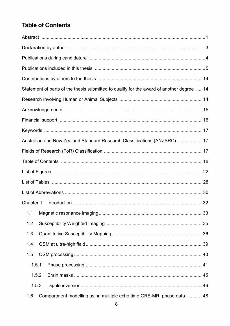
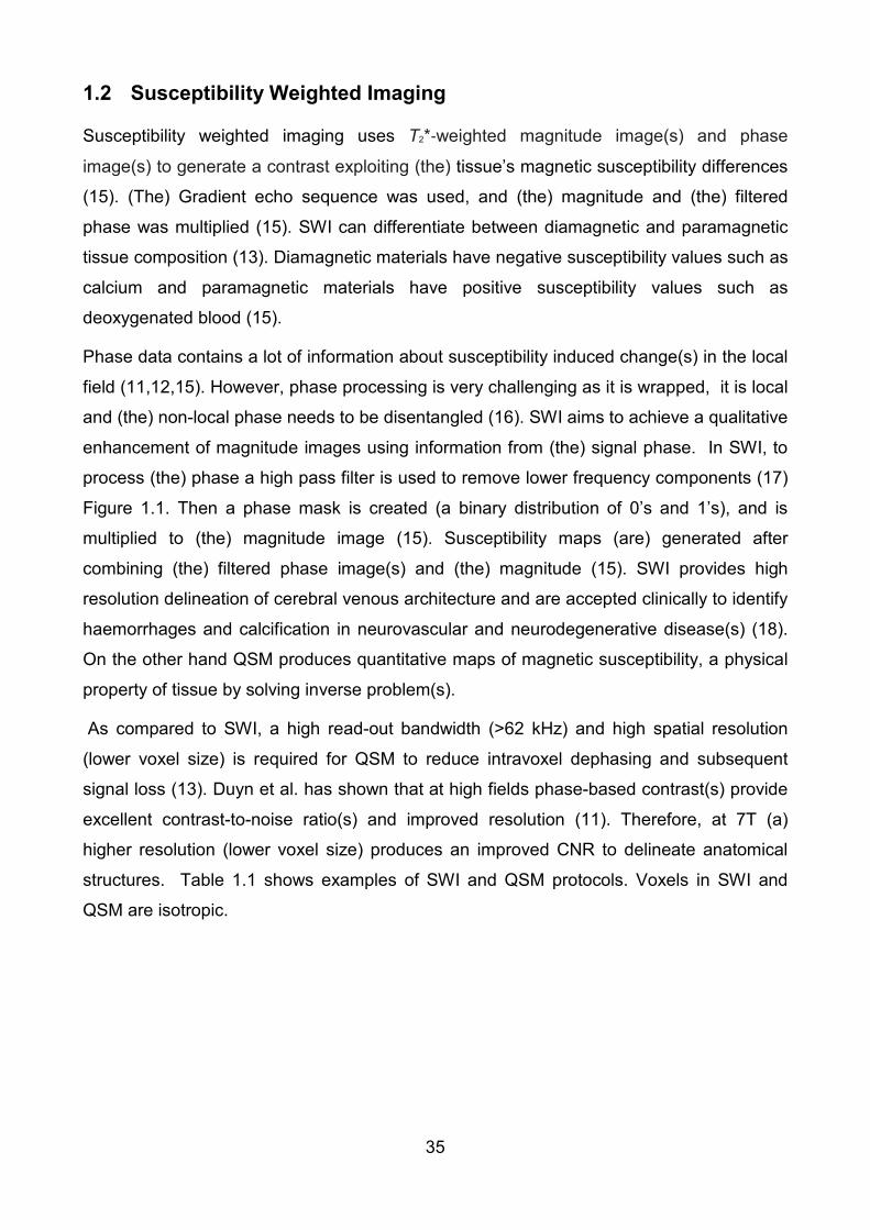
1.2 Susceptibility Weighted Imaging
Susceptibility weighted imaging uses T2*‐weighted magnitude image(s) and phase
image(s) to generate a contrast exploiting (the) tissue’s magnetic susceptibility differences
(15). (The) Gradient echo sequence was used, and (the) magnitude and (the) filtered
phase was multiplied (15). SWI can differentiate between diamagnetic and paramagnetic
tissue composition (13). Diamagnetic materials have negative susceptibility values such as
calcium and paramagnetic materials have positive susceptibility values such as
deoxygenated blood (15).
Phase data contains a lot of information about susceptibility induced change(s) in the local
field (11,12,15). However, phase processing is very challenging as it is wrapped, it is local
and (the) non-local phase needs to be disentangled (16). SWI aims to achieve a qualitative
enhancement of magnitude images using information from (the) signal phase. In SWI, to
process (the) phase a high pass filter is used to remove lower frequency components (17)
Figure 1.1. Then a phase mask is created (a binary distribution of 0’s and 1’s), and is
multiplied to (the) magnitude image (15). Susceptibility maps (are) generated after
combining (the) filtered phase image(s) and (the) magnitude (15). SWI provides high
resolution delineation of cerebral venous architecture and are accepted clinically to identify
haemorrhages and calcification in neurovascular and neurodegenerative disease(s) (18).
On the other hand QSM produces quantitative maps of magnetic susceptibility, a physical
property of tissue by solving inverse problem(s).
As compared to SWI, a high read-out bandwidth (>62 kHz) and high spatial resolution
(lower voxel size) is required for QSM to reduce intravoxel dephasing and subsequent
signal loss (13). Duyn et al. has shown that at high fields phase-based contrast(s) provide
excellent contrast-to-noise ratio(s) and improved resolution (11). Therefore, at 7T (a)
higher resolution (lower voxel size) produces an improved CNR to delineate anatomical
structures. Table 1.1 shows examples of SWI and QSM protocols. Voxels in SWI and
QSM are isotropic.

36
1.3 Quantitative Susceptibility Mapping
The main goal of computing susceptibility maps is to ascertain the sources causing field
perturbation. The field perturbation introduced by biological tissues may aid in
Figure 1.1 Flowcharts of processing steps of SWI (a) and QSM (b). (a) SWI combines both the magnitude and a filtered phase map in a multiplicative relationship to enhance image contrast(s). Minimum intensity projection (MIP) is commonly applied to highlight the veins. SWI flowchart adapted from Reichenbach et al. (b) There are two major steps involved in QSM: filtering (the) background phase and solving an inverse problem.
Table 1.1 Examples of SWI and QSM protocoles for the brain. Source: (13)

37
understanding tissue composition and structure. Quantitative susceptibility mapping is a
technique which resolves the local nuclear magnetic resonance (NMR) of the tissues with
varying magnetic susceptibility (10). Magnetic susceptibility can be defined as the degree
of magnetization an object experiences when placed in an external magnetic field (10).
Magnetic susceptibility can be defined as (19):
,M Hχ= (2.4)
where M is the induced magnetization, H is the applied magnetic field described in Am-
1, χ is the magnetic susceptibility and it is a dimensionless quantity. When an external
magnetic field oB is applied in z-direction to a sample with a magnetic susceptibility ( )rχ ,
the induced magnetization at any point r can be written as (19):
' ' 2 '
3 '05 3' ' '
3 ( )( ) ( )( ) ,4
z zz V
M r z z M rB r d rr r r r
µπ
− ∆ = − − −
∫ (2.5)
Equation (1.5) can be written as a convolution between ( )zM r and dipole response ( )G r :
0( ) ( ) ( ),z zB r M r G rµ∆ = ∗ (2.6)
where ( )G r is the Green’s function (20):
2
3
1 3cos 1( ) ,4
G rrθ
π−
= (2.7)
Lastly, change in (the) measured field is expressed using (a) forward modelling process is
defined as:
{ }10( ) ( ) ( ) ,zB r B FT k G kχ−∆ = ⋅ ⋅ (2.8)
where, ( )kχ is the Fourier transform of ( )rχ (12,19).
The notation can also be expressed as (13):
0 . * ,B B dχ∆ =measured (2.9)
where B∆ measured is measured field, 0 B is the main field strength, χ is the magnetic
susceptibility and d is the convolution kernel. Magnetic susceptibility can be calculated by
performing dipole deconvolution of the signal (16). All biological components such as iron,
myelin, and calcium induce a specific magnetic field perturbation at (a) microscopic level
which is reflected in the measured field (Figure 1.1). The measured field consists of field
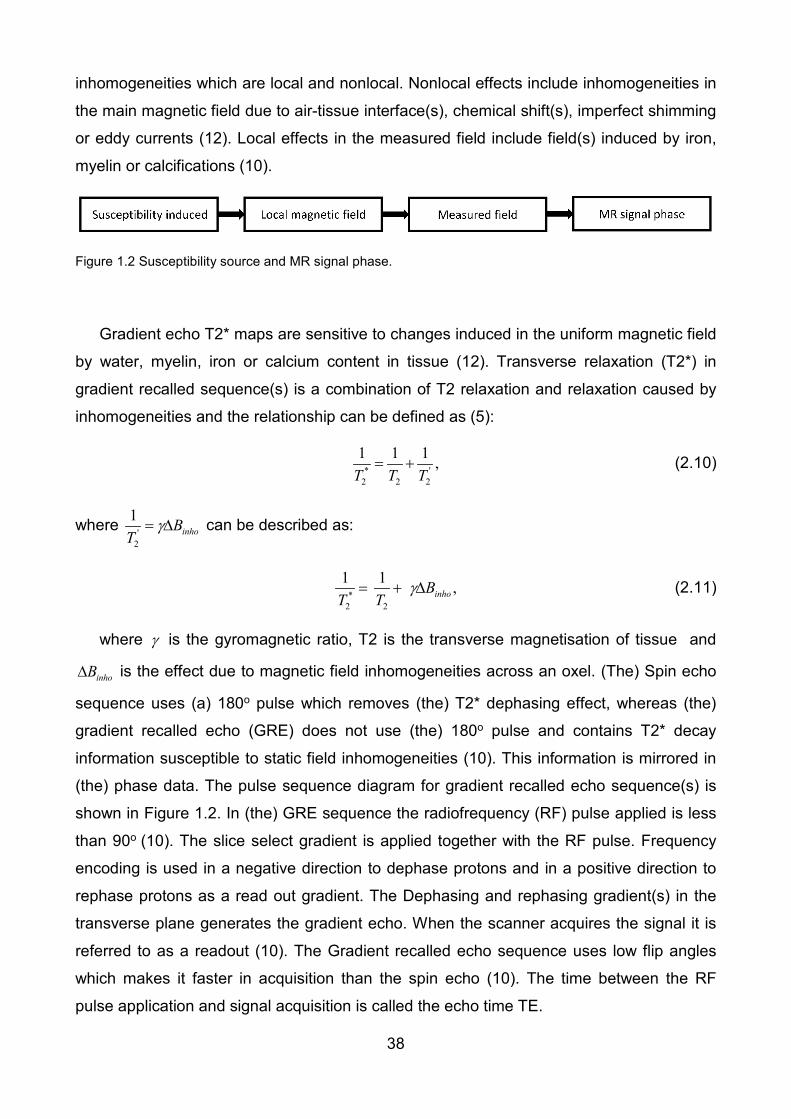
38
inhomogeneities which are local and nonlocal. Nonlocal effects include inhomogeneities in
the main magnetic field due to air-tissue interface(s), chemical shift(s), imperfect shimming
or eddy currents (12). Local effects in the measured field include field(s) induced by iron,
myelin or calcifications (10).
Gradient echo T2* maps are sensitive to changes induced in the uniform magnetic field
by water, myelin, iron or calcium content in tissue (12). Transverse relaxation (T2*) in
gradient recalled sequence(s) is a combination of T2 relaxation and relaxation caused by
inhomogeneities and the relationship can be defined as (5):
* '2 2 2
1 1 1 ,T T T
= + (2.10)
where '2
1inhoB
Tγ= ∆ can be described as:
*2 2
1 1 , inhoBT T
γ= + ∆ (2.11)
where γ is the gyromagnetic ratio, T2 is the transverse magnetisation of tissue and
inhoB∆ is the effect due to magnetic field inhomogeneities across an oxel. (The) Spin echo
sequence uses (a) 180o pulse which removes (the) T2* dephasing effect, whereas (the)
gradient recalled echo (GRE) does not use (the) 180o pulse and contains T2* decay
information susceptible to static field inhomogeneities (10). This information is mirrored in
(the) phase data. The pulse sequence diagram for gradient recalled echo sequence(s) is
shown in Figure 1.2. In (the) GRE sequence the radiofrequency (RF) pulse applied is less
than 90o (10). The slice select gradient is applied together with the RF pulse. Frequency
encoding is used in a negative direction to dephase protons and in a positive direction to
rephase protons as a read out gradient. The Dephasing and rephasing gradient(s) in the
transverse plane generates the gradient echo. When the scanner acquires the signal it is
referred to as a readout (10). The Gradient recalled echo sequence uses low flip angles
which makes it faster in acquisition than the spin echo (10). The time between the RF
pulse application and signal acquisition is called the echo time TE.
Figure 1.2 Susceptibility source and MR signal phase.

39
The phase data captures information on the induced field change (10) . The phase (ϕ )
reflecting inhomogeneities for echo time (TE) is defined as:
. . ,B TEϕ γ= − ∆ (2.12)
where γ is the gyromagnetic ratio and B∆ is the effect due to magnetic field
inhomogeneities. The susceptibility effects captured in the induced field can then be
calculated from equation(1.9). However, computing susceptibility from the equation is an
ill-posed inverse problem as inverse filtering will cause streaking artefacts in the magnetic
susceptibility maps due to zeros present on dipole at magic angle 54.7o. (12) Methods to
improve streaking artefacts are discussed in section 1.3.3.
1.4 QSM at (an) ultra-high field
QSM is a phase imaging technique (21). The tissue-specific magnetic field perturbation
information used to calculate susceptibility maps is reflected in phase data (21). Duyn et
al. has demonstrated that gradient-echo sequence at 7.0 tesla (7T) generates a strong
phase contrast within and between gray and white matter (11). The contrast is attributed to
local field variations in magnetic susceptibility which is potentially mainly due to iron
deposits. It infers that local field variations amplifies at ultra-high field(s) thus generating
strong phase contrasts (10).
Figure 1.3 2D Pulse sequence diagram for gradient recalled echo. RF is the radio frequency pulse, SLICE is the slice selection gradient, PHASE is the phase encoding gradient, READOUT is the readout gradient, ADC is the analog-to-digital converter, and SIGNAL is the signal acquired. The amplitude of the phase encoding gradient is changed to obtain different k-space lines.

40
A study ha(s) shown T2*-weighted images at 7T are more sensitive to susceptibility
contrast(s) as compared to 1.5T and can effectively divulge the details of microvasculature
for human brain tumours (22). It is also demonstrated that 7T is more sensitive to
anatomical details as compared to 3T (23). 7T also provides a higher sensitivity to
susceptibility-induced variations with (a) high SNR and high resolution (24). Therefore,
susceptibility maps calculated from phase data acquired at ultra-high field(s) become more
informative as the maps are more sensitive to human brain structures as compared to
lower fields. In this thesis mainly the motivation behind using the data acquired from ultra-
high field scanner(s) (7T) was high sensitivity to susceptibility-induced variations, high
SNR, and high resolution.
1.5 QSM processing
GRE T2* weighted sequence(s) is (are) used to generate QSM maps (10). QSM is a post-
processing technique and susceptibility maps can be generated by different methods (12).
In a basic processing pipeline (the) GRE phase and magnitude data is used. Mainly, the
susceptibility maps are influenced by (the) GRE phase data and thus categorized as
phase imaging method (16). A simple QSM pipeline shown in Figure 1.4 involved mask
generation(s), phase unwrapping, background field removal (tissue phase) and dipole
inversion(s) (susceptibility map(s)). Complex data is acquired from the scanner and then
separated into phase and magnitude (16). The complex data can be combined with the in-
built scanner coil combination method or can be combined outside the scanner. Magnitude
data can be used to generate mask(s), however it is also plausible to use phase
information for mask generation (10). (The) Mask is used to segment the brain for
background phase removal and susceptibility map generation. Then phase data is
processed to unwrap the phase and remove the background phase to compute tissue
phase (13). It is also plausible to perform phase unwrapping and background phase
removal in one step to obtain tissue phase(16). Finally, susceptibility map(s) is (are)
generated from (the) tissue phase. Phase processing, brain mask generation and dipole
inversion are the main steps in the QSM pipeline and are discussed in the following sub-
sections.

41
1.5.1 Phase processing
Since phase data depends on the bulk susceptibilities of different tissues, phase
processing is a crucial step in (the) QSM pipeline (25). Phase processing includes phase
unwrapping and background phase removal (10). Phase wrapping occurs because of the
phase measurement between +𝜋𝜋 to –𝜋𝜋. Numerous methods have been proposed for
phase unwrapping if implemented separately from background phase removal (12). Phase
unwrapping algorithms can be classified into spatial and temporal domains. In the spatial
phase, unwrapping (of) the phase difference between two neighbouring voxels is
calculated, whereas in the temporal phase unwrapping (the) phase difference between
echo times is utilized. Several spatial phase unwrapping methods are available (12). A
region growing spatial unwrapping path-based algorithm uses separate quality maps for
seed finding and unwrapping, and the quality maps include the information from both (the)
magnitude and (the) phase (26). Unwrapping is performed simultaneously in a number of
regions, and the seed(s) in the region grow outwardly (27). The limitation of this region
growing method is that unwrapping depends on the initial seed point. The initial seed
points are supposed to be in locally smooth regions, otherwise it affects the phase
unwrapping. Another three-dimensional quality map based unwrapping technique unwraps
the most reliable voxels first and the least voxels last (28). This method unwraps (the)
highest quality regions first and (the) lowest quality regions last. This technique relies on of
quality maps for unwrapping and if noisy voxels are chosen as high quality voxels, it can
influence unwrapping. An N-dimensional phase unwrapping method can unwrap the
Figure 1.4 Schematic illustration of the general QSM pipeline used to obtain susceptibility maps from raw
phase images acquired using gradient recalled echo magnetic resonance imaging sequences.

42
phase data of any dimension with an optimized cost function (29). It has been
implemented for 2D and 3D MRI data but can be implemented to any number of
dimensions. This method has been used in echo planar imaging (EPI) unwarping and
rapid, automated shimming applications in functional magnetic resonance imaging (fMRI).
The optimization method used in this approach is stuck in the local minimum after each
iteration. Therefore, this method being fast and easy to implement does not promise the
best solution. Phase unwrapping can also be performed using Laplacian-based methods
(30). In Laplacian-based methods, the Laplacian operator uses only trigonometric
functions of the phase and removes the components which are not part of the brain
following spherical mean value filtering (SMV) for background phase removal (31). This
method is fast and robust but background phase removal could not be performed
efficiently. Another Laplacian based method uses phase Laplacian outside the brain with
L2 norm minimisation (30). This fast and easy to implement method achieved phase
unwrapping and background phase removal effectively in one step. The spatial
unwrapping method fails to work effectively when the phase difference between adjacent
voxels is greater than 𝜋𝜋. Temporal unwrapping has an advantage over spatial unwrapping
in that it works even when the phase difference between adjacent voxels is greater than 𝜋𝜋
(12). The Temporal domain is useful in multi echo data where voxel-by-voxel unwrapping
is performed with short echo spacing (32) or unequal echo spacing (33). The Voxel-by-
voxel unwrapping method catalytic multi echo phase unwrapping scheme (CAMPUS) uses
the information in the multi echo gradient echo sequence with short interecho spacing (32).
The CAMPUS algorithm performed better than PhUN and the branch cut algorithm,
however the flow induced phase contributions can introduce errors in unwrapping as
shown in Figure 1.5 (4c-white arrow). Another voxel-by-voxel unwrapping method
unwrapping multi‐echo phase images with irregular echo spacings (UMPIRE) uses
unequal echo spacing so that no wraps can occur between the echo time and removing
(removes) any phase offsets computed. This method is fast and robust but it does not
when bipolar compensation is used. Ineffective phase unwrapping or any additional noise
originated at this step will be propagated in the QSM pipeline. Therefore, phase
unwrapping is a critical step in the QSM pipeline as it determines the quality of
susceptibility maps.

43
(The) Background field consists of nonlocal and local phase components (10) and the
Background field removal methods remove nonlocal field inhomogeneities. Various
methods have been suggested to remove the background field before or after phase
unwrapping (12). A k-space high pass filtering preserves local phase information but might
not be able to remove the background field effectively with a small filter size whereas
employing a large filter size can fail to detect details in the phase information for large
structures (34). Homodyne filtering can also be used to remove the background phase, but
using a small filter size might not remove the background phase completely and using a
Figure 1.5 Comparison of unwrapped phase images by (the) Catalytic multiecho phase unwrapping
Scheme (CAMPUS), phase unwrapping (PhUN), and the branch cut algorithms (of) four normal volunteers.
To avoid the cusp artefact observed in the scanner-combined phase images, these (phase) images were
derived from (the) complex division of echo 10 by echo 1 to give an effective echo time of 23.67ms. The
White arrow in (c-4) points to a few voxels incorrectly unwrapped by CAMPUS due to the violation of slow
flow assumption. The black arrows in row (d) and (e) points to areas where PhUN and the branch cut
algorithms failed to unwrap. Note that the phase images were scaled to the full gray scale range for better
visualization. Source:(32)

44
large filter size may lead to signal loss (15,35,36). Another method uses the Fourier
transform based field estimation method to evaluate geometry-induced field changes
introduced by air-tissue interface (35). This method is very computationally intensive and
hence the processing time is very long. A polynomial fitting is also used to remove the
background field that does not require phase unwrapping or masking (37). However, for
this method if moving window analytical estimation is not performed correctly it can
generate artefacts. Projection onto dipole fields (PDF) is considered as a reliable method
which is based on the assumption that the background field generated by the background
field dipoles is a harmonic function and the local field is nonharmonic (38). The same
assumption is exploited in a sophisticated harmonic artefact reduction for(of) phase data
(SHARP), using the spherical mean value property (39). There are two improved versions
of SHARP available: regularization enabled SHARP (RESHARP) and the variable radius
of the spherical kernel at the brain boundary (V-SHARP). RESHARP employs Tikhonov
regularization at the deconvolution stage of spherical mean value filtering to reduce noise
levels (40), while SHARP uses truncated single value decomposition (SVD). It was shown
in the results that truncated SVD generates more Gibbs artefacts than Tikhonov
regularization (40,41). V-SHARP uses a spherical filter with a different radius, and it
reduced artefacts close to boundaries as the filter size is small (and) close to boundaries
(41). Our work implemented iterative harmonic phase removal using the Laplacian
operator (iHARPERELLA), an integrated method to unwrap the phase and effectively
remove the background (30). Figure 1.6 shows that consistent results can be obtained
from HARPERELLA, PDF and V-SHARP. iHARPERELLA is easy to implement, fast,
robust and accurate (30).

45
1.5.2 Brain masks
Artefacts from the noisy regions such as air-tissue interfaces impacts the quality of
susceptibility maps (12,15,35). A study has also revealed that areas close to the skull and
background field from blood flow limited the accuracy of susceptibility maps (42). The
background field induced by artefacts can be reduced by masking such regions and
managing them separately (43). Therefore, generating masks is a crucial step as any
errors from local field variations can affect the quality of susceptibility maps. A study
demonstrated that masking out noisy regions can reduce artefacts and improve
susceptibility maps when a haemorrhage is present (44). It infers that masking plays an
Figure 1.6 Comparison of the background-removed phase and magnetic susceptibility obtained using
different phase processing methods. (A, B) Tissue phase images obtained using HARPERELLA [HARmonic
(background) PhasE REmovaL using the LAplacian operator]. (C, D) Tissue phase images obtained using
path-based phase unwrapping and V-SHARP (sophisticated harmonic artefact reduction for phase data with
varying spherical kernel sizes). (E, F) Tissue phase images obtained using path-based phase unwrapping
and PDF (projection onto dipole fields). (G, H) The Phase difference between the results obtained with
HARPERELLA and path-based phase unwrapping plus PDF. (I, J) Susceptibility maps derived from
HARPERELLA-processed phase images. (K, L) Susceptibility maps derived from phase images obtained
using path-based phase unwrapping and V-SHARP. (M, N) Susceptibility maps derived from phase images
obtained using path-based phase unwrapping and PDF. (O, P) The Difference between the susceptibility
maps obtained with HARPERELLA and path-based phase unwrapping plus PDF. Source:(30)

46
important role in computing the susceptibility maps specifically near air-tissue interfaces or
when motion is present.
Brain masking is defined as the region with a spatial distribution of 1’s and 0’s (12). The
area of interest in masking is represented by 1’s and the region outside the area of interest
is represented by 0’s. Masks can be produced by thresholding phase data or magnitude
data (26,45). Masks can be a whole brain mask or a structure specific mask. Masks can
be generated manually using a visualization software such as MIPAV (46) and carefully
referring to an atlas. In our work, while performing manual segmentation for the specific
regions such as caudate, putamen, gray matter or white matter we used an atlas for
anatomical reference (47). Masks can also be generated automatically using the Brain
extraction tool in FSL (FMRIB, University of Oxford) or FreeSurfer (29,48). One important
consideration is the registration of data to the FSL or Freesurface while extracting the
labels. Although Freesurfer is completely automated, manual editing can be performed at
particular steps to ensure the alignment of labels (48). Masks can also be used to perform
computations such as a frequency shift or susceptibility value calculation for the specific
region.
1.5.3 Dipole inversion
Magnetization at the voxel level can be signified as a magnetic dipole and thus the dipole
model is assumed to be representative of the influences within a voxel (49).The
assumption has been tested in phantom studies (50–52). The dipole approximation is
confirmed to work in high iron brain regions (53). The iron concentration showed a
correlation with susceptibility. However, it remains unclear whether the dipole
approximation holds inhomogeneous tissue (WM, GM) (12,54,55). The local field is the
convolution of susceptibility sources with the unit dipole at any point the space (12).
Therefore, magnetic susceptibility can be calculated by deconvolving the local magnetic
field with the magnetic field generated by a unit dipole (Equation(1.9)). A Three-
dimensional susceptibility matrix was Fourier transformed and multiplied element-by-
element (56). Using the Fourier transformation it was faster to compute magnetic
susceptibility as compared to integral-based methods (56). Moreover, complex and non-
local expressions become simple and local when computed in the Fourier domain (20).
The 3D deconvolution is an ill-posed inverse problem due to the presence of zeros on
the edges of the dipole and division by zeros would cause streaking artefacts which is the
biggest challenge for QSM algorithms as shown in Figure 1.7 (12). Several methods have

47
been proposed to solve this ill-posed inverse problem and reduce these steaking artefacts
(12). The QSM algorithms can be classified into single orientation based or multiple
orientation based (21). Several single orientation based methods have been proposed.
One way of reducing streaking artefacts is through regularization techniques.
Regularization techniques use prior information to solve ill-posed inverse problems (51).
The prior information can be extracted from the anatomy provided by an MRI.
Regularization techniques have been used to improve the streaking artefacts such as ℓ1-
regularized susceptibility mapping (57). A different Bayesian regularization approach uses
tissue priors from magnitude images to fill the missing information causing artefacts (54).
Another tissue prior method which uses information from magnitude and phase images to
improve the underestimation of susceptibility distribution is Morphology Enabled Dipole
Inversion (MEDI) (50,58). The limitation of tissue prior methods is its reliance on accurate
prior information. An iterative orthogonal and right triangular decomposition (iLSQR)
method uses the derivative relationship to evaluate susceptibility maps (59). The LSQR is
based on the bidiagonalization described by Golub and Kahan (60). It is shown that the
LSQR generated better results if the problem is ill-conditioned as compared to conjugate-
gradient algorithm (61). This method is fast, robust and easy to implement, and has shown
significant improvement over streaking artefacts. The Threshold-based k-space (TKD)
method applies the threshold in the k-space to reduce the streaking artefacts caused by
the zeros present at the magic angle (62). The TKD approach relies on the value of the
threshold chosen. If the value is too low the streaking artefacts will affect the quality of
susceptibility maps, and if the value is too high the susceptibility maps will show less
contrast (62). We have used Threshold-based k-space (TKD) in our work which includes
information from different angles (63). It is demonstrated that TKD information from two or
three orientations can improve the quality of susceptibility maps as compared to a single
orientation. This method is simple and fast to implement and has also shown a reduction in
artefacts (63).

48
When data is acquired from multiple orientations, oversampling fills the null regions at the
magic angle (54.70) (Figure 1.8) (64). Hence, streaking artefacts can be removed with
multiple orientation acquisition. However, one major limitation of multiple orientation
acquisition is the limited movement of the human head in the scanner which makes it an
impractical approach. The Calculation of susceptibility through multiple orientation
sampling (COSMOS) is considered to be a gold standard as it generates very high quality
susceptibility maps but it requires a minimum of 12 orientations data (64).
1.6 Compartment modelling using multiple echo time GRE-MRI phase data
GRE data has improved gray-white matter contrast by many times in magnitude and
phase (11). The contrast may possibly have originated from deoxyhemoglobin blood
(11,65), myelin (11,66), and iron (11,67,68). Several studies have suggested that contrast
Figure 1.7 Susceptibility map with streaking artefacts (a) and without streaking artefacts (b).
Figure 1.8 (a) The object is scanned at the first position. Then the object is rotated around the x-axis. (b) The
scan is repeated at the second orientation. The rotation-scanning process repeats until the required number
of rotations is reached. Subsequent rotations are not shown here. (c) The dipole response kernel function in
the Fourier domain (fixed with respect to the object) has zeros located on a pair of cone surfaces (the green
pair for the first sampling and the blue pair for the second sampling). The presence of these zeros makes the
inversion extremely susceptible to noise and they need to be avoided when possible. Sampling from two
orientations is insufficient because these two pairs of cone surfaces will still intercept, resulting in lines
of common zeros. Sampling from an appropriate third angle can eliminate all the common zeros in the dipole
kernels except the origin, which only defines a constant offset but does not change the relative susceptibility
difference between tissues in the image. Source:(64)

49
in GRE magnitude and phase images is also related to the orientation and global geometry
of white matter with respect to the main magnetic field at subcellular level (69–73). Another
study has demonstrated that myelin content and microstructure affects T2* maps in white
matter of the human brain at an ultra-high field (74). Moreover, it is also seen that tissue
constituents like iron-rich oligodendrocytes influence the MR phase data in white matter
(75).
Multi-echo GRE sequences have been used to study T2* decay in white matter across
echo time (76–78). Gradient echo multi echo sequences have been used to analyse T2*
decay as it is considered sensitive to capture the water exchange effects at shorter echoes
in white matter. Studies have successfully used T2* decay to evaluate myelin water
fraction (MWF) with a threepool model across echo time at 3T (76,79). The three pool
model consists of myelin water pool (my), myelinated axon water pool (ma), and a mixed
water pool (mx) as shown in Equation(1.13). The three pool model measured T2* decay
within seven parameters. Pool specific T2* ranges were fixed for my, ma and mx pools. A
number of iterations were performed to achieve optimum T2* endpoints with the minimum
error between fitting and the measured signal.
* * *2, 2, 2,( ) ,my ma mx
t t tT T T
my ma mx blS t A e A e A e A− − −
= + + + (2.13)
Where S is the magnitude signal as a function of time, Amy, Ama, and Amx represent the
amplitude of the signals arising from three water pools , Abl represents any residual
baseline signal, and T2*my, T2*ma, T2*mx are the relaxation rate for three water pools. The
limitation of the model was low SNR in MRI data. An improved model was proposed by
Gelderen et al. (Equation(1.14)). The study has also used a three-compartment model and
has indicated that the frequency shift associated with each compartment is induced by
varied myelin structure susceptibilities. It is shown that field strength affects SNR and thus
multi-compartment model values (78) in white matter.
* * *2,1 1 2,2 2,3 32 2
1 2 3( ) ,tR i f t tR tR i f tS t A e A e A eπ π− − − − −= + + (2.14)
Where S is the magnitude signal as a function of time, Ai is the amplitude, fi the off-
resonance frequency (in Hz) and R*2,i the relaxation rate of component i (R*2=1/T2*) . The
multi-compartment, when resolved at the voxel level, provides the compartment specific
(axonal, myelin and extracellular) distinct volume, frequency shifts, and T2* values in white
matter. This study has used single image acquisition which can increase the scan time and
single image acquisitions are more prone to motion artefacts. Sati et al. have investigated

50
how orientation can affect frequency shifts for compartments (80). The model used can be
described as:
*2,3 2
1( ) ,i itR jt f
iiS t Ae π− − ∆
==∑ (2.15)
where S(t) is the complex signal as function of time, j is the imaginary unit, Ai is the
amplitude, Δfi the frequency shift with respect to the local mean resonance frequency as
determined by subtracting the low-pass filtered phase, R*2,i the relaxation rate of the
component i. This model considered two complex valued compartments and one real-
valued compartment. The study concluded that frequency shift compartments are affected
by the magnetic field effect induced by myelin, axonal, and interstitial water with respect to
the main magnetic field. Another complex value based three compartment method was
proposed which did not require the background phase removal method (81). This method
fits complex data to the complex model. The model is as follows:
* * *2, 02, 2,( 1/ 2 ) (2 )( 1/ 2 ) ( 1/ 2 )( ) ( ) ,my my bgax ax ex exT i f t i f t iT i f t T i f t
my ax exS t A e A e A e eπ π ϕπ π− + ∆ ∆ −− + ∆ − + ∆= + + (2.16)
where, An is the amplitude, T2*,n is the relaxation time, Δfn is the frequency shift of
my(myelin), ax(axonal), and ex(extracellular), Δfbg is a background frequency offset term
that originates from the macroscopic (nonlocal) field inhomogeneity, and 𝜑𝜑0 is the phase
offset. The method is robust and the results obtained from this method were more stable
as compared to previous methods. Considering the anisotropic nature of myelin,
Sukstanskii et al. proposed a new three-compartment model which accounts for the
orientation effects of myelinated axons (82). The proposed three compartments are:
axonal, myelin and extracellular, in which axonal and myelin water frequency shifts are
affected by anisotropic magnetic susceptibility, and myelin water is non-monoexponential
(82).
Multi-compartment modelling has been applied to assess the demyelination in multiple
sclerosis. A reduction or complete loss of myelin water has been observed in chronic
demyelinated MS lesions (83,84). Since the three water pools are associated with
particular T2*, multi-compartment fitting of T2* decay (including frequency shift) could
provide information about MS-related abnormalities. A study in MS patients has
implemented a three component model with the following equation (85):
* * *2,1 1 2,2 2 2,3 (2 )( 1/ 2 ) ( 1/ 2 ) ( 1/ )
1 2 3( ) ,gi f tT i f t T i f t T tS A e A e A e e π ϕπ π +− + ∆ − + ∆ −= + + (2.17)

51
where, An is the amplitude, T*2,n is the relaxation time, and Δfn is the frequency shift of
the component n, which is defined relative to the interstitial water frequency fg , and 𝜑𝜑 is
the phase offset. This study established that the three compartment model could
characterize myelin loss based on the frequency shifts. The results exhibited a good
correspondence with clinical findings. Furthermore, performing myelin water imaging
(MWI) at 7T brings additional high SNR gain which is important for in depth myelin
assessment (86).
This suggests that thecomposition and arrangement of microstructure influences the
GRE signal. The compartmentalization of the GRE signal over the echo time may provide
a new diagnostic tool to investigate microstructure on the gradient echo contrast (87).
However, how tissue composition and orientation influences gray matter were not studied
and it is shown that tissue composition influences susceptibility maps such as iron
deposits (53). This thesis focuses on analysing tissue structure influences in gray matter
regions with a multi-compartment model. QSM has been seen as a promising measure for
tissue assessment as compared to phase mapping (88). Therefore, we decided to perform
compartment modelling on susceptibility values. The phase unwrapping, background
phase removal and susceptibility map calculation algorithms were available in STI
Suitev2.0 (30). STI Suitev2.0 is fast and easy to implement. Chapter 3 aims at the multi-
exponential fitting of GRE data in human brain regions across echo time to quantify the
tissue.
1.7 Utility of ultra-high field MRI
Anatomical structural details with high resolution has always been of great interest in both
clinics and research MRIs. T1, T2, and T2* sequences have been widely implemented on
1.5T and 3T (2,5,83,89). With the availability of ultra-high field scanners, it is possible to
obtain a high SNR. Duyn et al. has also demonstrated that the SNR of the GRE phase
signal is improved as the field strength is increased (11).
It is demonstrated that multi-compartment analysis requires a high SNR (79). Geldren
et al. has demonstrated a multi-compartment fitting of T2* decay at 3T and 7T. The study
showed that compartments at 3T were less separable as compared to 7T. The potential
reason could be the lower SNR at 3T (78). 19 echoes were acquired for the study with TE1
= 2.7ms and an echo spacing of 2.35ms. The choice of echo time was made to detect
slow water exchange in white matter in T2* mapping (74). It is not evaluated yet how SNR
affects gray matter compartments for different field strengths. We extended our work from

52
Chapter 3 to analyse multi-compartment fittings at 3T and 7T in Chapter 5 to assess
frequency maps over echo time for both gray and white matter. For this study frequency
shift maps were computed. Frequency shift maps can be computed by scaling multiple
echo phase data with respective echo time but we calculated frequency maps from
susceptibility maps. A recent study has shown that frequency maps when calculated from
susceptibility maps have reduced the effect of local field inhomogeneities effect (90).
Therefore, in Chapter 5 frequency maps assessed are computed from susceptibility maps.
Cronin et al. has proposed that methodological differences can affect susceptibility
maps across echo time (91). He suggested that Laplacian unwrapping fails to perform
around strong susceptibility sources like cerebral microbleeds (CMBs). It is still not clear
how different processing pipelines can affect compartment modelling. Therefore, we
decided to use two different methods to analyse any methodological effects on multi-
compartment modelling. Different phase processing pipelines have been discussed in
section 1.3.1. An integrated Laplacian based method for phase and unwrapping and
background phase removal (iHARPERELLA) (30), and path based phase unwrapping
method were used with iLSQR (61) for susceptibility map calculation at the end. All of the
algorithms are available in STI Suitev2.0.
1.8 GRE in cerebral cortex
As discussed in section 1.3.3, orientation plays an important role in the computation of
susceptibility maps (64). Although multiple orientation yields good quality susceptibility
maps, it is still not feasible to achieve the desired human head rotations in the scanner.
Several single orientation methods have been proposed to reduce the streaking artefacts
caused by the null signal region (see section 1.3.3) (12). Sati et al. has shown that the
orientation with respect to the main magnetic field influences compartment values (80).
However the impact of the orientation in compartments has not been studied for gray
matter.
The orientation effects in gray matter and white matter were studied using two different
methods (threshold-based k-space (TKD) and iLSQR) (61,62). The threshold-based k-
space (TKD) method as discussed in section 1.3.3 uses two or three orientations and
improves the susceptibility maps as compared to the single orientation method (62), while
iLSQR is a single orientation method which removes streaking artefacts significantly (30).
Frequency shifts were computed from the susceptibility maps computed from TKD and
iLSQR it is suggested by Wu et al. that this method reduces nonlocal effects (90).
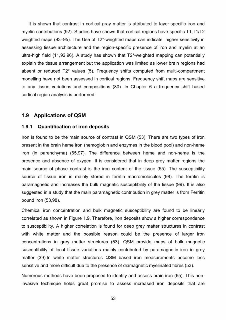
53
It is shown that contrast in cortical gray matter is attributed to layer-specific iron and
myelin contributions (92). Studies have shown that cortical regions have specific T1,T1/T2
weighted maps (93–95). The Use of T2*-weighted maps can indicate higher sensitivity in
assessing tissue architecture and the region-specific presence of iron and myelin at an
ultra-high field (11,92,96). A study has shown that T2*-weighted mapping can potentially
explain the tissue arrangement but the application was limited as lower brain regions had
absent or reduced T2* values (5). Frequency shifts computed from multi-compartment
modelling have not been assessed in cortical regions. Frequency shift maps are sensitive
to any tissue variations and compositions (80). In Chapter 6 a frequency shift based
cortical region analysis is performed.
1.9 Applications of QSM
1.9.1 Quantification of iron deposits
Iron is found to be the main source of contrast in QSM (53). There are two types of iron
present in the brain heme iron (hemoglobin and enzymes in the blood pool) and non-heme
iron (in parenchyma) (65,97). The difference between heme and non-heme is the
presence and absence of oxygen. It is considered that in deep grey matter regions the
main source of phase contrast is the iron content of the tissue (65). The susceptibility
source of tissue iron is mainly stored in ferritin macromolecules (98). The ferritin is
paramagnetic and increases the bulk magnetic susceptibility of the tissue (99). It is also
suggested in a study that the main paramagnetic contribution in grey matter is from Ferritin
bound iron (53,98).
Chemical iron concentration and bulk magnetic susceptibility are found to be linearly
correlated as shown in Figure 1.9. Therefore, iron deposits show a higher correspondence
to susceptibility. A higher correlation is found for deep grey matter structures in contrast
with white matter and the possible reason could be the presence of larger iron
concentrations in grey matter structures (53). QSM provide maps of bulk magnetic
susceptibility of local tissue variations mainly contributed by paramagnetic iron in grey
matter (39).In white matter structures QSM based iron measurements become less
sensitive and more difficult due to the presence of diamagnetic myelinated fibres (53).
Numerous methods have been proposed to identify and assess brain iron (65). This non-
invasive technique holds great promise to assess increased iron deposits that are

54
associated to various neurological disorders such as Alzheimer’s disease, Parkinson’s
disease, and multiple sclerosis (100,101).
Iron accumulation increases over the life span and hence the mean susceptibilities. Figure
1.10 shows that QSM is sensitive to detect the changes in age-related iron deposition with
two different methods (102). Susceptibility values for caudate, putamen, substantia nigra,
red nucleus, and globus pallidus are higher in elderly participants as compared to young
participants, however it is not true for frontal white matter, thalamus and dentate nucleus. It
can therefore be deduced that the susceptibility measure can estimate any age-related
variations in iron distribution for most of the grey matter regions.
Figure 1.9 Correlation of bulk magnetic susceptibility with measured iron concentration. The line represents
the regression of all data points and the dotted lines indicate the 95% confidence intervals. Source:(53)

55
1.9.2 Traumatic brain injury
QSM is sensitive to the paramagnetic property of deoxyhaemoglobin venous abnormality
in Traumatic brain injury (TBI) (16,103). The Phase difference between venous blood spins
Figure 1.10 Mean ± SEM of average susceptibility in ppm computed by the two methods (ℓ1-regularized
QSM, top; ℓ2-regularized QSM, bottom) for each ROI in the young and elderly groups. Source: (102) and
LEM means standard error from the mean.
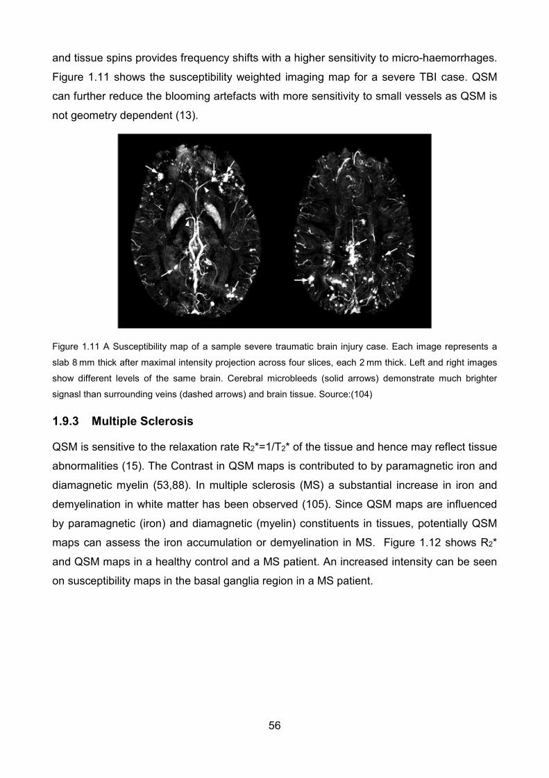
56
and tissue spins provides frequency shifts with a higher sensitivity to micro-haemorrhages.
Figure 1.11 shows the susceptibility weighted imaging map for a severe TBI case. QSM
can further reduce the blooming artefacts with more sensitivity to small vessels as QSM is
not geometry dependent (13).
1.9.3 Multiple Sclerosis
QSM is sensitive to the relaxation rate R2*=1/T2* of the tissue and hence may reflect tissue
abnormalities (15). The Contrast in QSM maps is contributed to by paramagnetic iron and
diamagnetic myelin (53,88). In multiple sclerosis (MS) a substantial increase in iron and
demyelination in white matter has been observed (105). Since QSM maps are influenced
by paramagnetic (iron) and diamagnetic (myelin) constituents in tissues, potentially QSM
maps can assess the iron accumulation or demyelination in MS. Figure 1.12 shows R2*
and QSM maps in a healthy control and a MS patient. An increased intensity can be seen
on susceptibility maps in the basal ganglia region in a MS patient.
Figure 1.11 A Susceptibility map of a sample severe traumatic brain injury case. Each image represents a
slab 8 mm thick after maximal intensity projection across four slices, each 2 mm thick. Left and right images
show different levels of the same brain. Cerebral microbleeds (solid arrows) demonstrate much brighter
signasl than surrounding veins (dashed arrows) and brain tissue. Source:(104)

57
1.9.4 Brain Tumour
QSM can differentiate between tumor-related calcification and blood products (106). It has
also been found to be sensitive to glioblastoma and glioblastoma with oligodendroglial
components (106). Figure 1.13 shows images of a glioblastoma patient with
oligodendroglial components. Figure 1.13(j) shows a hyper intense region indicating blood
components and a hypo intense region representing calcification.
Figure 1.12 Representative R2* maps (top row) and quantitative susceptibility maps (bottom row) of two 29-
year-old individuals, a healthy control subject and a MS patient. Note increased (more paramagnetic)
susceptibility in the basal ganglia in the MS patient. Differences are most evident in the putamen (arrow,
0.049 vs 0.092 ppm). Image window settings were identical: R2* mapping, from 0 (black) to 40 sec−1(white);
QSM, from −0.1 (black) to 0.25 ppm (white). Source:(105)
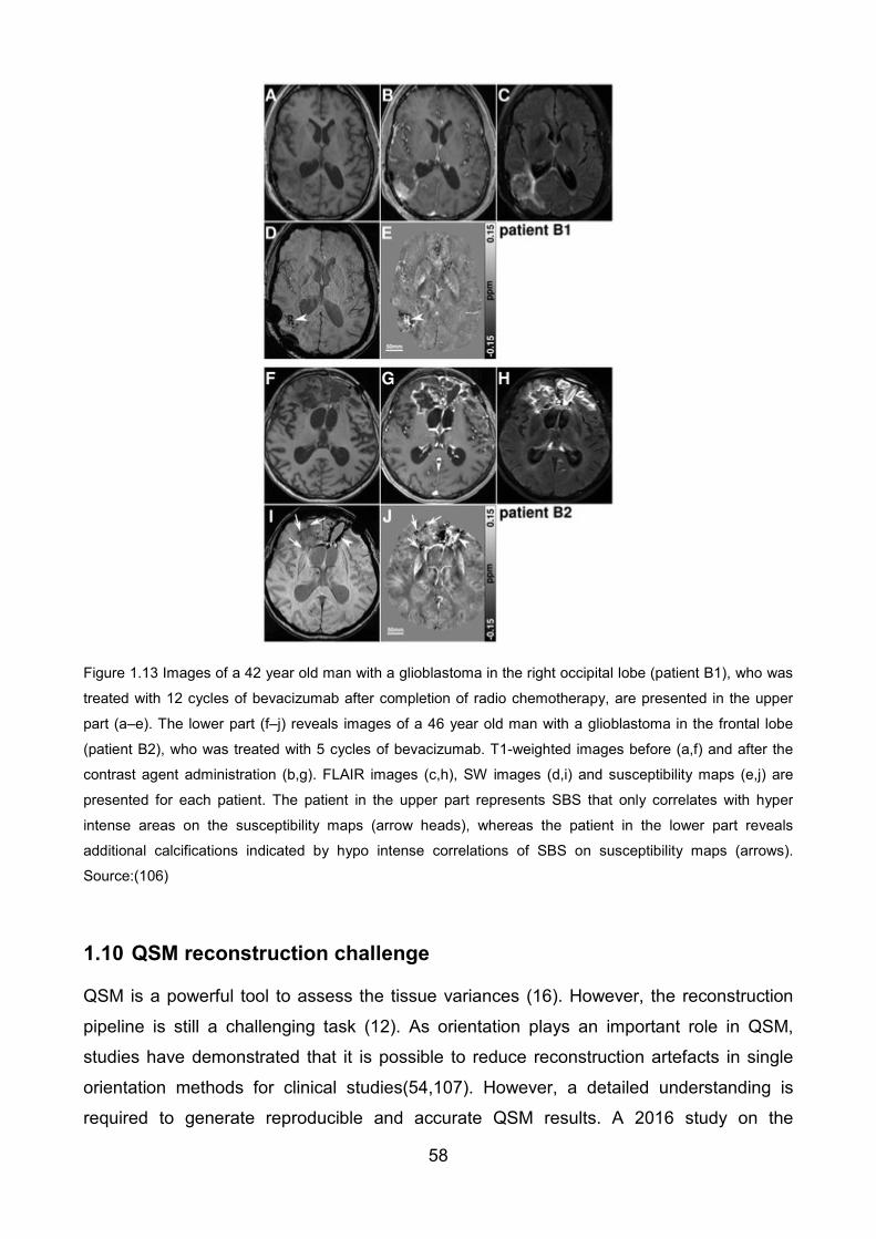
58
1.10 QSM reconstruction challenge
QSM is a powerful tool to assess the tissue variances (16). However, the reconstruction
pipeline is still a challenging task (12). As orientation plays an important role in QSM,
studies have demonstrated that it is possible to reduce reconstruction artefacts in single
orientation methods for clinical studies(54,107). However, a detailed understanding is
required to generate reproducible and accurate QSM results. A 2016 study on the
Figure 1.13 Images of a 42 year old man with a glioblastoma in the right occipital lobe (patient B1), who was
treated with 12 cycles of bevacizumab after completion of radio chemotherapy, are presented in the upper
part (a–e). The lower part (f–j) reveals images of a 46 year old man with a glioblastoma in the frontal lobe
(patient B2), who was treated with 5 cycles of bevacizumab. T1-weighted images before (a,f) and after the
contrast agent administration (b,g). FLAIR images (c,h), SW images (d,i) and susceptibility maps (e,j) are
presented for each patient. The patient in the upper part represents SBS that only correlates with hyper
intense areas on the susceptibility maps (arrow heads), whereas the patient in the lower part reveals
additional calcifications indicated by hypo intense correlations of SBS on susceptibility maps (arrows).
Source:(106)

59
reconstruction challenges in QSM has analysed various QSM algorithms (108). After
comparing various QSM algorithms, it was concluded that different QSM algorithms
exhibited methodological differences and this makes extracting the true susceptibility
values challenging, an implication for clinical translation.

60
Chapter 2 Research aims and hypothesis
The Aim of this thesis is to develop new methods by exploiting the information contained in
susceptibility maps. A study has shown that frequency shifts from multi-echo gradient echo
sequences vary with echo times (69). It is also shown that the GRE phase signal in white
matter consists of frequency shifts from axonal, myelin and extracellular water which can
be identified with a multi-compartment model (80,82). The studies mentioned had three
compartment information which includes the size of the compartment, R2* or T2*, and the
frequency shift. The studies have implemented different compartment models to assess
the influences on gradient echo signals through compartments. The Quality of the fit is
used to evaluate how perfectly the measured data points are explained by the
compartment model. The Different number of compartments can be used in the modelling
techniques.
Compartment modelling has been performed only in the white matter (78,80,82,85). It
is still unknown whether or why the susceptibility or frequency shift (which can be
calculated from susceptibility maps) varies over the echo time. Theoretically, magnetic
susceptibility should not vary over the echo time as it is a physical quantity. Additionally, it
has not been studied whether compartmentalization of susceptibility maps or frequency
maps indicate any influences of tissue composition or arrangement. We analysed how
echo-time dependence in QSM could potentially reveal the tissue variation through
compartmentalization in human brain regions. Parameterization of GRE signals may
possibly reflect the health of tissue which might be useful in detecting any early
abnormalities in neurological and neurodegenerative diseases.
Research has established that phase imaging offers 10-fold improvement in contrast-
noise-ratio (CNR) as compared to GRE and magnetization-prepared rapid gradient-echo
(MPRAGE) magnitude images, and it further improves approximately 100-fold at ultra-
high fields (11). The research gap was to investigate how GRE signal compartments are
influenced by the field strength and how using different processing pipelines affects
compartments. We analysed multi-compartment models in human brain regions at 3T and
7T with two different processing pipelines. This study enables us to decide the usability of
compartments with the field strength and different methodologies.

61
Susceptibility maps computed from a single orientation and multiple orientations differ
in the quality, suggesting orientation plays an important role in QSM (109). The Research
question was to study the influence of the orientation on compartmentalisation. It was
explored how compartments vary with data acquired at different angles in human cerebral
cortex. The Multi-compartment model was used to analyse compartments in different
cortical regions. The Single orientation and TKD (with orientation information from three
acquisitions in different angles) were used to compute frequency shifts. It was analysed if
a single orientation is informative (enough) to implement the multi-compartment model as
compared to multiple orientations.
Aim 1: Echo-time dependent quantitative susceptibility mapping contains information on tissue properties - Chapter 3
Hypothesis
It has been shown in a study that frequency shift maps derived from phases are echo time
dependent in white matter (80,82). A three compartment signal model (interstitial water,
intra-axonal water and myelin water) was used to explain the non-linear trend in
susceptibility (80). The frequency maps or susceptibility maps have not been studied over
the echo time in grey matter. We suggested the susceptibility maps in grey matter regions.
Although compartmental frequency shift contributions have been used to explain the trend
in white matter, the trend in QSM response has not been studied in either gray or white
matter (73,80,82) . We proposed to study the information contained in the temporal trend
by analysing the mapped magnetic susceptibility as a function of echo time from gradient
recalled data acquired at 7T.
Aim 2: Contribution of cortical layer cytoarchitecture to quantitative susceptibility mapping - Chapter 4
Hypothesis
Our results from Chapter 3 suggested that it is possible that chemical composition and
structural arrangement influence susceptibility maps over the echo time. To further study
the effect of tissue composition, we computed magnetic susceptibility maps obtained from
multiple echo time magnetic resonance imaging data over the echo time for series of
voxels selected along the line of gennari, and just above and just below the line of gennari.
The proposition was to analyse how different or similar the susceptibility maps are along
the line of gennari, above the line of gennari and below the line of gennari as the
linecontains highly myelinated axons affecting susceptibility values (110).
62
Aim 3: Field strength influences on the gradient recalled echo MRI signal compartment frequency shifts - Chapter 5
Hypothesis
The Signal to noise ratio is directly proportional to the main magnetic field (11). Field
perturbations are influenced by field strength and are reflected in the gradient recalled
echo magnetic resonance imaging (GRE-MRI) signals (11). Mapping of phase at 7T has
been shown to provide as much as a 10-fold increase in gray-white matter contrast in
comparison to the contrast in magnitude images (11). In Chapter 3 the susceptibility over
the echo time has been explored in human brain regions at 7T. However, the influences of
the magnetic field strength on susceptibility or frequency maps were not clear. Therefore,
in Chapter 5 the impact of field strength is studied in the frequency shifts which are further
compartmentalised in selected human brain regions.
Aim 4: Evaluation of multi-echo QSM in the brain cortex using an ultra-high field - Chapter 6
Hypothesis
Results from Chapter 5 indicated that methodological and field strength differences
influence frequency shift compartments, however consistent results can be generated with
any method or field strength used. We extended our frequency map analysis in the human
Cerebral Cortex in Chapter 6. As it is demonstrated that orientation affects frequency
maps and susceptibility maps (12,69), we planned to assess the effect of orientation in
frequency maps generated from QSM maps, and the measurements were made at
different angles. It was explored how frequency shifts computed from different
methodologies can be used to assess cortical regions.

63
Chapter 3 Echo-time dependent quantitative susceptibility mapping contains information on tissue properties
Magnetic susceptibility has been considered echo time independent. However, this
assumption is not true if the anisotropicity of specific tissues is taken into account. The
field orientation dependent field perturbations will induce an anisotropic magnetic
susceptibility. The effect will vary with the structure, composition and arrangement of the
tissue. However, it is still unclear which factors influence the magnetic susceptibility at the
voxel level. In this chapter we investigated susceptibility maps over echo time, and
analysed if the susceptibility trends reflects any changes in chemical composition and
tissue structure.
3.1 Abstract
Magnetic susceptibility is a physical property of matter that varies depending on chemical
composition and abundance of different molecular species. Interest is growing in mapping
of magnetic susceptibility in the human brain using magnetic resonance imaging
techniques, but the influences affecting the mapped values are not fully understood. We
performed quantitative susceptibility mapping on 7 Tesla (T) multiple echo time gradient
recalled echo data and evaluated the trend in 10 regions of the human brain. Susceptibility
maps were plotted across echo time in the caudate, pallidum, putamen, thalamus, insula,
red nucleus, substantia nigra, internal capsule, corpus callosum, and fornix.
We implemented an existing three compartment signal model and used optimization to fit
the experimental result to assess the influences that could be responsible for our findings.
The susceptibility plots across echo time are different for different brain regions, and sub-
segmentation of specific regions suggests that differences are likely to be attributable to
variations in tissue structure and composition.
Using a signal model, we verified that across echo time a nonlinear behaviour in
experimentally computed susceptibility within imaging voxels may be the result of the
heterogeneous composition of tissue properties. Decomposition of voxel constituents into
meaningful parameters may lead to informative measures that reflect changes in tissue
microstructure.

64
3.2 Introduction
Quantitative susceptibility mapping (QSM) has been developing rapidly as a magnetic
resonance imaging (MRI) tool (12,51,111). In QSM, maps of regional changes in the
physical constant, magnetic susceptibility, are obtained. Although both magnitude and
phase images are known to be influenced by the magnetic properties of tissue, gradient
recalled echo (GRE) phase images have been shown to contain excellent contrast and, at
a field strength as low as 1.5T, can reveal anatomic structures not visible on
corresponding magnitude images (25). QSM relies on acquired phase images to solve for
voxel susceptibilities. At the ultra-high field (7T), as much as a 10-fold improvement in
phase image contrast relative to magnitude image contrast can be achieved (11). Several
studies have verified that QSM-based approaches are sensitive to tissue composition,
resulting in image contrasts that reflect tissue structural changes (31,107). In fact, QSM
has been used to monitor iron deposition (53,112), quantify contrast agent uptake
(113,114), identify multiple sclerosis lesions (105,115), and map cerebral microbleeds
(116) and intracranial calcification (42).
The echo time of GRE-MRI data acquisitions can manually be varied to influence the
phase contrast achieved in GRE-MRI data. Researchers have demonstrated an echo time
of the average of the grey and white matter T2* (transverse relaxation time in the presence
of field inhomogeneities) results in the maximum phase contrast between grey and white
matter in a normal participant (11,117). Additionally, it was shown that white matter
frequency shift maps generated from phase images, the input to the QSM processing
pipeline, are influenced by echo time (69). Constituents such as iron and cellular
constituents such as oligodendrocytes within voxels affect susceptibility isotropically or
anisotropically, and have been suggested to influence the phase response with echo time
in a nonlinear fashion (75). Decades ago Chu et al. showed shifts in the nuclear magnetic
resonance signal frequency due to bulk susceptibility and suggested that complicated
structures with multiple susceptibility compartments are likely the cause of non-intuitive
changes in the signal over the echo time (118). Hence, the pattern of echo time
dependence of QSM maps may provide insight into tissue structure and the effects of
central nervous system disorders on brain tissue constituents.
However, the echo time dependence on various brain regions, particularly grey matter
regions, has not been evaluated as a function of the mapped value of susceptibility. To
study the regional dependence of QSM on echo time, we evaluated the QSM result at an
ultra-high field across a range of echo times. Very short echo spacing GRE-MRI data were

65
used to evaluate susceptibility values in 10 brain regions and in specific sub-regions. We
then sought to parameterise the mapped susceptibility curves over echo time by
compartmentalising the MRI signal into multiple susceptibility constituents. We formulated
signal compartments using the plane wave formulation, as has been done in previous
studies.
Initial work on water-fat separation using MRI data across echo time considered a two
compartment model containing water and fat pools (119,120). In this model a fixed
frequency shift between water and fat was used in the computations. Each compartment
was expressed as a complex valued plane wave having an amplitude, induced frequency
shift and relaxation time. Compartment contributions at the voxel level were obtained
through an optimisation procedure. The approach was adopted in four white matter studies
and considered three instead of two frequency shift compartments associated with myelin
water, restricted water such as those within axons, mobile water such as those in
extracellular spaces and in cerebrospinal fluid (80). The effect of iron has not been
considered in these models, however the plane wave formulation, the basis of each signal
compartment, is theoretically capable of accounting for large amplitude susceptibility
constituents. The first modelling approach considered one real valued compartment
(restricted water) and two complex valued compartments incorporating frequency shifts
due to two susceptibility effects (78). This approach was shown not to be as robust in
fitting white matter frequency shift trends as a model wherein each of the three signal
compartments were allowed to account for separate susceptibilities (80). The three
susceptibility compartment model was recently applied in a multiple sclerosis cohort in
which white matter lesions are known to form and showed a frequency shift change
associated with a so-called white matter lesion compartment (85). A more complicated
expression for myelinated axon contribution has also been developed as a replacement for
the plane wave based expression for myelin contribution, with the aim of expressing signal
dependence on white matter orientation with respect to the imaging field (121). In our work
we opted to investigate the utility of the second model (three susceptibility compartments
and no fibre orientation dependence) as the alignment of myelinated axons with respect to
the imaging field is not necessarily resolvable, or applicable, in all brain regions studied.
Instead of assigning names to compartments, we took the general approach of
investigating how mapped susceptibility compartments vary in various brain regions known
to have differences in cell density, packing arrangements, myelination and iron
accumulation. For example, we considered brain regions such as the pallidum, red

66
nucleus, substantia nigra and putamen known to contain high iron concentrations (65,122),
whereas the caudate and thalamus have not been described to accumulate high levels of
iron. Furthermore, we investigated how susceptibility compartments change in the
substantia nigra and pallidum sub-regions, all of which are known to have different
cytoarchitectures. Our work promotes the use of susceptibility across echo time in brain
studies, thereby we refer to the method as temporal quantitative susceptibility mapping
(tQSM).
3.3 Methods
3.3.1 Data acquisition
Ethics was granted through the University of Queensland human ethics committee. In vivo
brain imaging (five healthy adult volunteers: two females aged 30 and 32, and three males
aged 31, 34 and 41) sessions were conducted on a 7T whole-body MRI research scanner
(Siemens Healthcare, Erlangen, Germany) with a 32 channel head coil (Nova Medical,
Wilmington, USA). A 3D gradient recalled echo non-flow compensated scan was acquired
with the following parameters: TE1 = 2.04ms, echo spacing = 1.53ms, 30 echoes, TR =
51ms, flip angle = 15°, voxel size = 1mm × 1mm × 1mm and matrix size = 210 × 168 ×
144.
Figure 3.1 Illustration of the pipeline used to compute quantitative susceptibility maps. Individual channel data were processed using STI Suite and combined into a single image at the very end.

67
3.3.2 Data reconstruction pipeline
A number of QSM processing pipelines have been developed to extract susceptibility from
GRE-MRI data (102,109,123), which includes phase unwrapping, background phase
removal and the solution to the field-to-source inverse problem. Several phase unwrapping
and background removal techniques have been proposed (38,54,124). Advances have
resulted in improvements in the quality of susceptibility information across the entire brain.
In practice, the field-to-source inverse problem is solved by the deconvolving tissue phase
with a dipole kernel (125–127). The problem is ill-posed due to the presence of zeros in
the kernel, which in the past resulted in unwanted streaking artefacts (64,107). Recently
developed methods have been able to reduce the confounding effects of such artefacts
(50,59).
Data were acquired from 32 channels and each channel was individually processed
prior to combining images (128). The combined images were a weighted average of the
individual channels. The magnitude image of each channel was used to form a channel
mask using the BET tool provided as part of MIPAV (http://mipav.cit.nih.gov/). The result
was read into MATLAB® (The MathWorks, Inc., Natick, Massachusetts, United States)
and binarised. individual channel masks were stored for use in the STI Suite
(http://people.duke.edu/~cl160/) processing package to compute spatial variations in
magnetic susceptibility. STI Suite calculates susceptibilities with respect to the mean
susceptibility of the region studied, which in our case was the whole brain. The QSM
pipeline is schematically illustrated in Figure 3.1 . In brief, individual raw phase data were
processed using iHARPERELLA provided as part of STI Suite (30,31,41). iHARPERELLA
was recently shown to lead to results as good as V-SHARP (129). The combined magnetic
susceptibility map was calculated as the average of individual channel susceptibility maps
using iLSQR available in STI Suite. The iLSQR output was mapped over echo times,
denoted as tQSM.
3.3.3 Manual region-of-interest selection
Manual segmentation was performed using a number of different echo time 7T magnitude
images based on clarity of structures identified in Figure 3.2, namely the caudate,
pallidum, putamen, thalamus, internal capsule, red nucleus, insula, corpus callosum,
substantia nigra and fornix. The segmentation of each ROI was guided by a human brain
atlas (47). The instruction was to segment regions such that segmentation boundaries
were clearly confined to the region, and not touching adjacent brain regions. This

68
approach produces a higher level of confidence for each region. ROIs were drawn using
MIPAV, and saved in the NIFTI format. A Matlab script was used to binarise ROI values,
resulting in region masks.
A second level segmentation was performed on three regions. The pallidum was
segmented into internal and external regions, the substantia nigra was segmented into
compact and reticular regions, and the insula was segmented into anterior and posterior
regions. These sub-regions were chosen as they are known to have different
cytoarchitectures and cell densities.
3.3.4 Mapping of susceptibility across echo time
Segmentation was performed on each hemisphere where relevant. The values were then
averaged across hemispheres and repeated for each echo time. This formed susceptibility
data for each participant over the echo time. Mean susceptibility values are plotted against
echo time, and standard deviations within each region are shown as well.
3.3.5 Multi-compartment contributions to susceptibility
Three models with three signal compartments each have been used to describe the non-
linear nature of the MRI frequency shift in white matter. In other studies signal
compartments have been referred to as contributions from intra-axonal space, myelin and
interstitial space. In the first model two signal compartments contain a frequency shift
Figure 3.2 Illustration of the location of the ten human brain regions-of-interest used to assess changes in
magnetic susceptibility.
69
component and the other accounts for magnitude signal decay only (78). The second
model employs independent frequency shifts for all compartments (80). The third model
incorporates a non-plane wave based function for the myelin contribution (121). The
additional complexity for the myelin signal was developed for white matter and we primarily
deal with grey matter. Therefore, we used the second model, which was recently applied
to multiple sclerosis data (81), and ignored fibre orientation as we primarily deal with grey
matter wherein neuron structure is vastly different to the relatively highly myelinated and
aligned cylindrical axons of white matter. Each signal compartment of an image voxel is
assumed to be describable using an amplitude modulated plane wave formulation:
*2,
( t )( ) ( ) ,
( ) 1, 2, 3,n
in n
tT
n n
S t A t e
A t A e n
ω φ+
−
=
= = (4.1)
where n is the signal compartment, ω defines the angular frequency and φ is a phase
shift. Notably, the induced change in angular frequency is a function of the induced change
in magnetic field, as defined by the Larmor equation ( Bω γ∆ = ∆ , where γ is the
gyromagnetic ratio). Furthermore, the amount of magnetic field change is determined by
the magnetic susceptibility ( χ ) of the substance (notably, 0B Bχ∆ = where 0B is the
reference field or static field of the scanner). The relationship 0B Bχ∆ = in the MRI context
holds only when changes due to susceptibility are confined to a voxel. Since we consider
effects within voxels, which are small spread out constituents with relatively small
susceptibility, we may assume that field change is local and 0B Bχ∆ = holds. We can justify
this in two ways. Firstly, a field produced by a dipole (commonly used susceptibility source
representation in QSM) decays at a rate 1/r2, where r represents distance away from the
centre of the dipole. If we consider microscale effects to be responsible for a change in the
magnetic field, then the extent of these changes decay on the microscale as well.
Secondly, Chen et al. simulated the induced field distribution within voxels and showed an
extent of a few micrometres at most from axonal structures which were less than 5
micrometres in size (130). Hence, we assume field changes due to microscale effects are
contained within millimetre scale voxels, and a dipole representation for individual
compartments can be avoided. With this in mind, Equation (3.1) can be used to define the
measured complex signal:
1 0 2 0 3 0* * *
2,1 2,3 2,31 2 3( ) ,
t t ti B t i B t i B tT T TS t A e A e A e
γχ γχ γχ− − − − − −
= + + (4.2)

70
The formulation of Equation (3.2) has nine parameters: 1A , 2A , 3A , 1 2 3, ,χ χ χ , *2,1T , *
2,2T
and *2,3T . Previously, the 2-norm of the residual formed by subtracting the right-hand-side of
Equation (3.2) from ( )S t was used and minimised based on an initial guess and brute
force searching for an optimal solution within the vicinity of the initial guess was performed
in an iterative manner. We opted for a robust method of optimising for the nine
parameters, thereby we implemented in MATLAB® the global optimisation method called
differential evolution (131), which was used to fit the temporal evolution of QSM curves
after values were averaged across all participants and each of the brain regions studied.
Through empirical testing we found that a cost function based on the argument was able to
produce better fits than the approach adopted in previous work. Hence, we minimised the
following cost function:
* * *2,1 2,2 2,3
* * *2,1 2,2 2,3
2
1 1 1 0 2 2 0 3 3 0
1 0
1 1 0 2 2 0 3 3 0
sin( ) sin( ) sin( )1( ) tan ,
cos( ) cos( ) cos( )
m m m
m m m
t t tT T TM
m m mM m t t t
m m T T Tm m m
A e B t A e B t A e B tf t
B tA e B t A e B t A e B t
γχ γχ γχχ
γγχ γχ γχ
− − −
−
− − −=
+ +
= −
+ +
∑ (4.3)
where 1 2 3 1A A A+ + = , M is the number of echo points of data collected, ( )mtχ are
reconstructed susceptibility values from experimental data at each echo time m output
from iLSQR, and the equation can be derived starting from Equation (3.2), applying Euler’s
formula and calculating the phase based on the expanded equation. The scaling 0 mB tγ
was applied to convert the phase to a susceptibility prior to subtracting it from the mapped
value of susceptibility ( ( )mtχ ). We initialised values for1
A , 2
A and 3
A in (0,1) randomly
and we imposed 1 2 3 1A A A+ + = within the optimisation algorithm. In the differential evolution,
algorithm values for1
, 2
and 3
were constrained to ( 610 , 610 ), that is the magnitude
of the value was not allowed to exceed 1ppm. Via empirical testing, we found
compartment T2* to be quite insensitive to changes across compartments, which is likely
due to how the cost function is formulated (i.e. Equation(3.3)), whilst this was not the case
for the magnetic susceptibility value. Hence, we computed the voxel T2* through an
optimisation procedure by initialising to a random value in the interval (20, 40ms). these
values were not constrained through the iterations, but we did restrict them to take positive
values only. We set the number of initial parameter states to 500 and ran 20,000 iterations,
the scaling factor (F) was set to 0.9 and a 20% cross over (CR) between parameter
estimates was allowed at each iteration using the DE/rand/1/bin variant of the differential
evolution algorithm. We repeated each run 10 times to confirm the convergence to a

71
reproducible estimate of parameters. Careful consideration has been taken to avoid
overfitting, as discussed in our recent work (132).
3.4 Results
3.4.1 tQSM curves
We mapped magnetic susceptibility across the entire brains of five participants from data
acquired on a human 7T MRI scanner and extracted values for ten brain regions.
Supporting Figure III provides example magnitude images and susceptibility maps at echo
times of 3.57ms, 15.81ms and 31.11ms. Figure 3.3 (caudate, internal capsule, red
nucleus, corpus callosum) and Figure 3.4 (thalamus, pallidum, substantia nigra, putamen,
fornix and insula) provide the tQSM curves. The mean values across the five participants
are represented as the thick solid line, and plus and minus one standard deviation bands
are shown using dashed lines. From these results we can conclude that tQSM curves vary
across brain regions. We sub-segmented particular brain regions to study the influence of
tissue cytoarchitecture variations on the tQSM curve.
The substantia nigra consists of compact and reticular parts (133). The compact part
has relatively large multipolar pigmented neurons (diameter in the range 25-45
micrometres; 300,000 to 550,000 neurons) with long and spine poor dendrites extending
into the reticular region. The reticular region consists of large multipolar non-pigmented
neurons (mean diameter around 25 micrometres; 260,000 to 280,000 neurons) having
long thick infrequently branching, aspiny dendrites, which are densely covered with
synaptic contacts. Additionally, it has been shown that the reticular part of the substantia
nigra generally contains more iron than the compact part (133). Figure 3.5 (a) provides the
results for the compact and reticular parts of the substantia nigra. The positive
susceptibility shift present from reticular to compact results may be suggestive of an
increase in neuron density and/or pigmentation, and may also be associated with different
levels of iron. Increased neuron density increases the number of magnetic field
perturbations within imaging voxels, which may be interpreted as increased magnetic
susceptibility constituents within voxels (130).
The pallidum is composed of external and internal segments having different
cytoarchitectures (133). We manually segmented the pallidum into external (containing as
many as 1.46 million neurons) and internal segments (around 310,000-350,000 neurons)
and Figure 3.5(b) provides the result. A positive shift in the susceptibility curve with an
expected increase in neuron density can also be observed.

72
The anterior insula has large pyramidal cell layers and a lack of development of a
granular layer results in a well-defined cytoarchitecture resembling frontal cortical structure
Type I, while the posterior insula has thick and parvicellular granular layers similar to the
parietal cortical structural Type III (134). The anterior and posterior sub-segmentation
results for the insula are provided in Figure 3.5(c). Interestingly, a different trend in the
mapped susceptibility response for the anterior and posterior regions is present in
comparison to sub-regions of the substantia nigra and pallidum (compare Figure 3.5(c) to
Figure 3.5(a) and Figure 3.5(b)). The distinct deviation of the two curves may be caused
by the presence of agranular structures towards the anterior region and granular structures
towards the posterior region. These findings imply tissue cytoarchitecture may play a role
in tQSM curve formation. Such a result may be useful in detecting and monitoring changes
in tissue cytoarchitecture, and measurable changes may play a role in various
neurodegenerative brain diseases and disorders.
3.4.2 Parameterisation of signal compartments
Table 3.1 provides the results for the ten brain regions investigated via fitting of values
used to parameterise the three susceptibility compartments, and Table 3.2 summarises
the results for the pallidum, insula and substantia nigra sub-regions. Supporting Figures I
and II provide the result fitted across echo time which are averaged across all participants.
Figure 3.3 tQSM results for (a) caudate, (b) internal capsule, (c) red nucleus and (d) corpus callosum.
Individual plots show the response for each participant (thin solid lines) along with the group mean (thick
solid line) and standard deviation (dashed lines). We found a trend in susceptibility values with echo time,
and the trend varies with region selected.

73
The adjusted R2 value is representative of the quality of fit achieved. For nine out of the
ten regions studied, the fitting process resulted in an adjusted R2 greater or equal to 0.93,
implying a very good quality of fit. A plot of each fitted curve is provided as supporting
information. For the pallidum a good fit was not obtained (R2 = 0.42). Two reasons are
plausible for this result. Firstly, the three compartment model may not have sufficient
degrees of freedom to be able to explain the trend in the tQSM curve (i.e. require
additional terms). Secondly, the model assumes plane waves can be used to explain each
signal compartment, which may not appropriately describe the signal behaviour observed
in the experimental data. In Table 3.2 results for internal and external regions of the
pallidum are provided with R2 = 0.99 and R2 = 0.82 respectively. Both the internal and
external regions contain a very similar susceptibility compartment (0.074ppm and
0.075ppm, 1.4% difference) and two slightly different susceptibility compartments
(0.033ppm versus 0.036ppm and 0.129ppm versus 0.137ppm resulting in 9.1% and 6.2%
differences). Interestingly, the pallidum has similar compartment susceptibilities as well
(0.080ppm, 0.037ppm and 0.14ppm). This suggests that segmentation of the brain regions
into sub-regions can potentially lead to improved compartment fitting.
Sub-segmentation of the insula into anterior and posterior regions did not result in
better model fitting (adjusted R2 of 1.00 and 0.96 versus 0.99), which is reasonable since
the quality of the fit for the insula was already very good. It may be that tissue
heterogeneity within the insula results in some destructive cancellation of compartment
signals. This is evidenced by vast susceptibility differences across the anterior and
posterior regions, as given in Table 3.2, and these values are also different to those
calculated for the insula. Signal compartments may thereby be decomposable into smaller
and smaller regions, which may result in increasing difficulty in interpreting model
parameters.

74
As already mentioned, the pallidum and substantia nigra contain similar neuronal cell
bodies (133). The largest compartment of the substantia nigra has a susceptibility of
0.03ppm, the value of which is present as the second largest compartment of the internal
region, and as the smallest compartment of the external region of the pallidum.
Furthermore, the second largest compartment of the substantia nigra has a susceptibility
of 0.07ppm, which is present as the largest susceptibility compartment of the internal
region and second largest susceptibility compartment of the external region of the
pallidum.
Figure 3.4 tQSM results for (a) thalamus, (b) pallidum, (c) substantia nigra, (d) putamen, (e) fornix and (f)
insula. Individual plots show the response for each participant (thin solid lines) along with the group mean
(thick solid line) and standard deviation (dashed lines). We found a trend in susceptibility values with echo
time, and the trend varies with region selected.
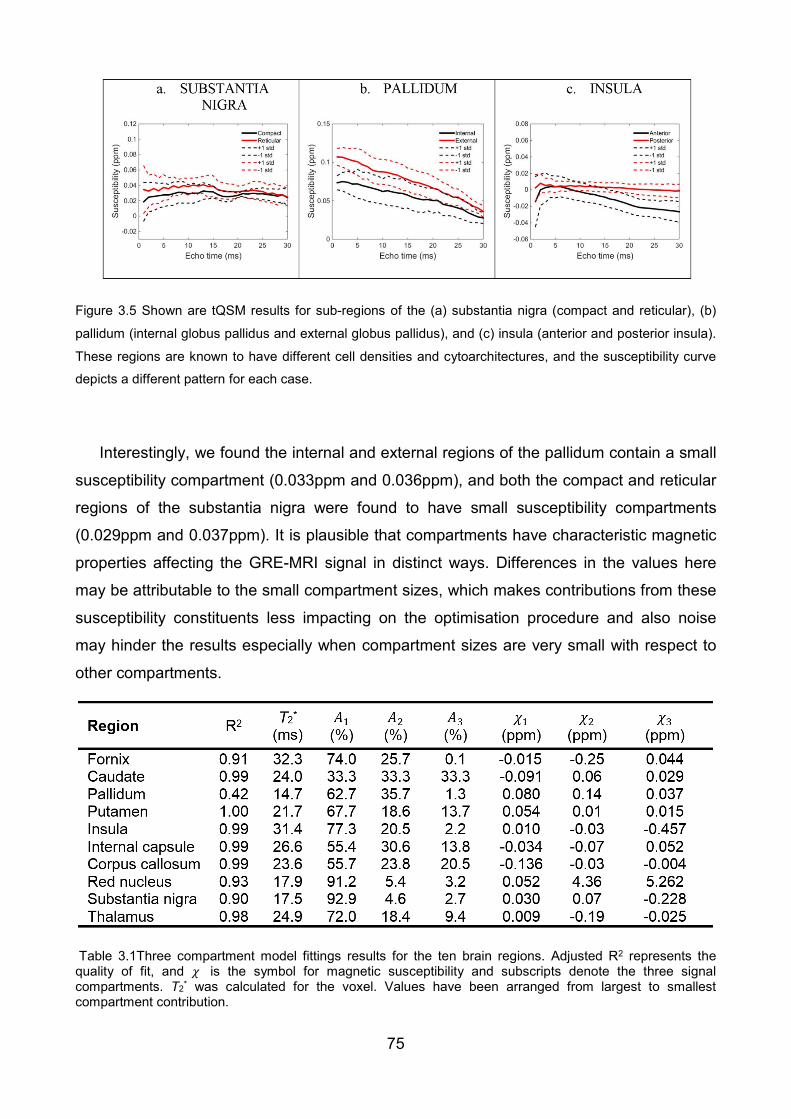
75
Interestingly, we found the internal and external regions of the pallidum contain a small
susceptibility compartment (0.033ppm and 0.036ppm), and both the compact and reticular
regions of the substantia nigra were found to have small susceptibility compartments
(0.029ppm and 0.037ppm). It is plausible that compartments have characteristic magnetic
properties affecting the GRE-MRI signal in distinct ways. Differences in the values here
may be attributable to the small compartment sizes, which makes contributions from these
susceptibility constituents less impacting on the optimisation procedure and also noise
may hinder the results especially when compartment sizes are very small with respect to
other compartments.
Figure 3.5 Shown are tQSM results for sub-regions of the (a) substantia nigra (compact and reticular), (b)
pallidum (internal globus pallidus and external globus pallidus), and (c) insula (anterior and posterior insula).
These regions are known to have different cell densities and cytoarchitectures, and the susceptibility curve depicts a different pattern for each case.
Table 3.1Three compartment model fittings results for the ten brain regions. Adjusted R2 represents the quality of fit, and 𝜒𝜒 is the symbol for magnetic susceptibility and subscripts denote the three signal compartments. T2* was calculated for the voxel. Values have been arranged from largest to smallest compartment contribution.

76
The red nucleus is known to contain large amounts of iron in comparison to the brain in
general (65,122). The threecompartment fitting resulted in susceptibilities of 0.052ppm,
4.369ppm and 5.262ppm in proportions of 91.3%, 5.5% and 3.2% respectively. In
essence, the signal is dominated by a small susceptibility compartment and affected by a
small but high susceptibility compartment (8.7% of the signal component). The size and
sign of the susceptibility implies the presence of a high magnetic susceptibility constituent,
which may be a marker of iron load. High susceptibility compartments within the red
nucleus of 4.36ppm (5.4%) and 5.262ppm (3.2%) can potentially be combined into one
compartment to account for the likely presence of iron.
Figures 3.6 and 3.7 show the standard deviation of magnetic susceptibility computed
based on magnetic susceptibility variations within brain regions. The combined result for
participants is shown after individual variances were pooled prior to calculating the
standard deviation. Figure 3.3, Figure 3.6, and Figure 3.4 and Figure 3.7 , can be
compared directly. We may note that the standard deviation based on participant
differences is generally larger than the standard deviation due to variations in
susceptibilities within the brain regions. Furthermore, the region-based variation appears
to maintain a fairly consistent window (of) echo time (i.e. standard deviations do not fan
out with longer echo times), implying adverse effects such as noise unlikely play a role in
the mean estimate of magnetic susceptibility. The regions which were sub-segmented into
sub-regions (substantia nigra, pallidum and insula in Figure 3.5 and Table 3.2) also show a
larger standard deviation, as more influences contribute to the measurements.
Table 3.2 Three compartment model fittings for the sub-segmented regions (SN stands for substantia nigra
and GP stands for globus pallidus). Adjusted R2 represents the quality of fit, and 𝜒𝜒 provides the calculated
value of the magnetic susceptibility across the three compartments. T2* was calculated for the voxel. Values
have been arranged from largest to smallest compartment contribution.

77
3.5 Discussion
Our work assesses quantitative susceptibility mapping across echo time. By studying ten
brain regions, we have been able to establish that the mapped value of susceptibility
changes with echo time. Interestingly, frequency shift maps are also shown to be a
function of echo time in white matter (69), and recently the presence of iron and
oligodendrocytes were suggested to produce a non-linear response with echo time (75). It
is already explained by Haacke et al. that a change of field (dB0) is not a function of echo
time, only the phase evolves with echo time (15). Therefore, the change in phase reflects
intrinsic tissue variations.
White matter volumes, known as highly myelinated fibres, are present not only in the
fornix, internal capsule, and corpus callosum, but also in the caudate (53,135,136). The
presence of negative valued susceptibilities within these brain regions is possibly a
measure of white matter contribution. This has also been observed in a study on the
corpus callosum exploring changes in frequency shift images across echo time (85).
The fornix, internal capsule and corpus callosum brain regions have echo time
dependent curves which are always negative. Notably, the contribution and magnetic
susceptibility value of each signal compartment influences the amplitude and shape of the
curves, which we deduce by comparing the susceptibility curves from these three brain
regions over the echo time. Wharton and Bowtell studied fibre-orientation contrast in
Figure 3.6 Standard deviation of the mapped magnetic susceptibility within regions across the ten brain
regions plotted over echo time: (a) fornix, (b) caudate, (c) putamen and (d) internal capsule. Solid line is the
mean magnitude signal and dashed lines represent one standard deviation from the mean.

78
gradient echo MRI, wherein they show effects on the frequency shift across echo time
curve due to the angle made between white matter and the magnetic field of the scanner
(69). They showed both a change in amplitude of the frequency shift curve, and also a
change in the shape of the curve. Frequency shifts mapped over echo time did not change
sign, that is, they were consistently negative. Based on our results and those by Wharton
and Bowtell, we can conclude that magnetic field orientation plays an important role in the
values obtained using susceptibility mapping. Since the susceptibility over the echo time
value in white matter is influenced by field orientation, the estimated compartment values
should be influenced as well.
The caudate and the putamen are cytoarchitecturally similar structures with small
neuronal cell bodies (137). It has also been established that the putamen contains larger
amounts of iron than the caudate, and iron deposition increases with age (39,53,98). We
found that both the caudate and putamen have similar susceptibility compartments. The
second largest compartment of the caudate and the largest compartment of the putamen
Figure 3.7 Standard deviation of the mapped magnetic susceptibility within regions across the ten brain
regions plotted over echo time: (a) corpus callosum, (b) red nucleus, (c) thalamus, (d) insula, (e) pallidum
and (f) substantia nigra. The Solid line is the mean magnitude signal and dashed lines represent one
standard deviation from the mean.
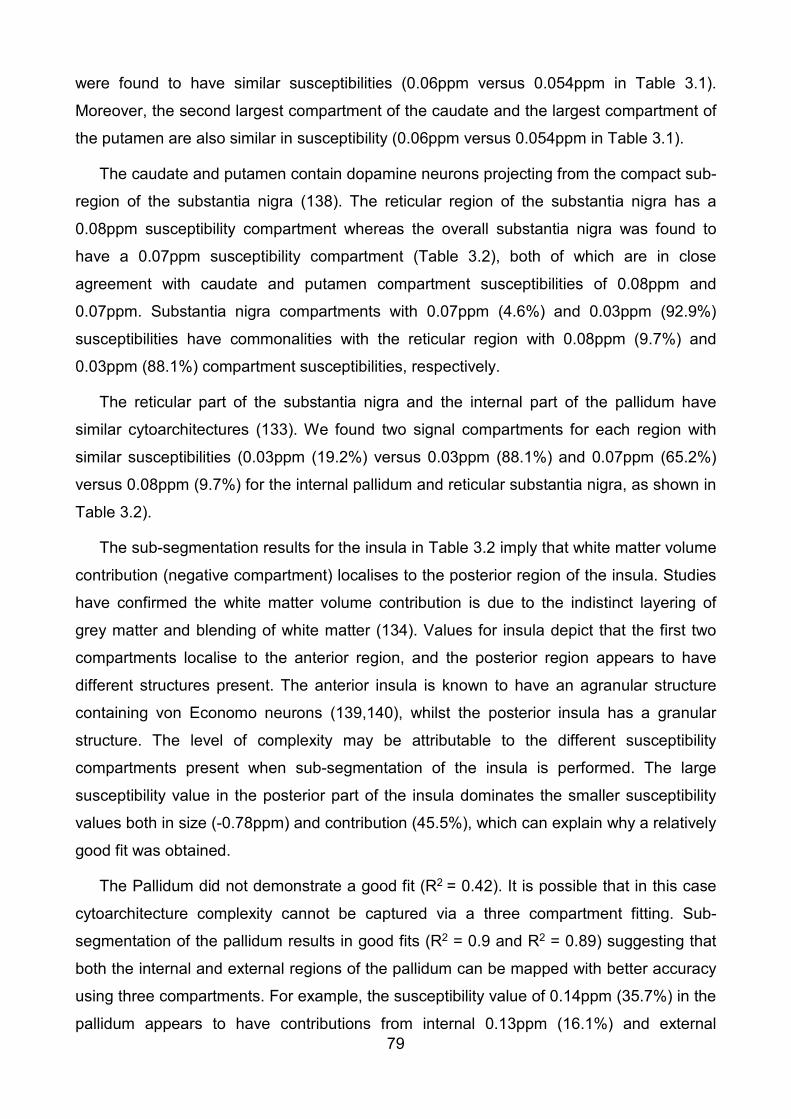
79
were found to have similar susceptibilities (0.06ppm versus 0.054ppm in Table 3.1).
Moreover, the second largest compartment of the caudate and the largest compartment of
the putamen are also similar in susceptibility (0.06ppm versus 0.054ppm in Table 3.1).
The caudate and putamen contain dopamine neurons projecting from the compact sub-
region of the substantia nigra (138). The reticular region of the substantia nigra has a
0.08ppm susceptibility compartment whereas the overall substantia nigra was found to
have a 0.07ppm susceptibility compartment (Table 3.2), both of which are in close
agreement with caudate and putamen compartment susceptibilities of 0.08ppm and
0.07ppm. Substantia nigra compartments with 0.07ppm (4.6%) and 0.03ppm (92.9%)
susceptibilities have commonalities with the reticular region with 0.08ppm (9.7%) and
0.03ppm (88.1%) compartment susceptibilities, respectively.
The reticular part of the substantia nigra and the internal part of the pallidum have
similar cytoarchitectures (133). We found two signal compartments for each region with
similar susceptibilities (0.03ppm (19.2%) versus 0.03ppm (88.1%) and 0.07ppm (65.2%)
versus 0.08ppm (9.7%) for the internal pallidum and reticular substantia nigra, as shown in
Table 3.2).
The sub-segmentation results for the insula in Table 3.2 imply that white matter volume
contribution (negative compartment) localises to the posterior region of the insula. Studies
have confirmed the white matter volume contribution is due to the indistinct layering of
grey matter and blending of white matter (134). Values for insula depict that the first two
compartments localise to the anterior region, and the posterior region appears to have
different structures present. The anterior insula is known to have an agranular structure
containing von Economo neurons (139,140), whilst the posterior insula has a granular
structure. The level of complexity may be attributable to the different susceptibility
compartments present when sub-segmentation of the insula is performed. The large
susceptibility value in the posterior part of the insula dominates the smaller susceptibility
values both in size (-0.78ppm) and contribution (45.5%), which can explain why a relatively
good fit was obtained.
The Pallidum did not demonstrate a good fit (R2 = 0.42). It is possible that in this case
cytoarchitecture complexity cannot be captured via a three compartment fitting. Sub-
segmentation of the pallidum results in good fits (R2 = 0.9 and R2 = 0.89) suggesting that
both the internal and external regions of the pallidum can be mapped with better accuracy
using three compartments. For example, the susceptibility value of 0.14ppm (35.7%) in the
pallidum appears to have contributions from internal 0.13ppm (16.1%) and external

80
0.12ppm (57.3%) regions, since the compartment contributions average to 36.7%, which is
close to the overall contribution within the pallidum (35.7%). The 0.08ppm susceptibility
compartment appears to be present in both internal and external regions as well, with
susceptibilities of 0.07ppm. However, the percentages do not equate here, which may be
due to the largest compartment having a compensating effect as part of the fitting process.
That is, the fitting procedure based on three compartments was not able to obtain a good
fit hence the largest compartment contribution may deviate from reality.
The thalamus contains a heterogeneity of cell nuclei, and the complexity of the
structure can lead to measures appearing isotropic by nature (141). We may therefore
expect to map a smaller amplitude tQSM curve in the thalamus as destructive cancellation
at the voxel level due to induced field changes at the microscale can occur. That is, the
change in magnetic field within a voxel from which susceptibility is indirectly deduced
depends on the complex interactions of microscopic field changes, which is likely to
appear more uniform or isotropic in terms of induced field change as tissue complexity
increases. On the other hand, the more consistently anisotropic the microstructures are
within a voxel, the larger the measurable susceptibility effect that can be expected (102).
The corpus callosum is an example of a highly anisotropic cytoarchitecture, and the
largest signal compartment does have a large negative susceptibility value (Table 3.1).
Hence, the inclusion of many cell types within voxels may artificially lead to a smaller
susceptibility response, even though the actual susceptibility of the tissue compartments
may not change. Effectively, this is because susceptibility is derived from an indirect
measure of field change. It is therefore reasonable that different cellular morphologies and
their arrangement lead to differing changes in the imaging field, which can be mimicked by
changing the size of the magnetic susceptibility along with the amount of compartmental
contribution. A future approach of overcoming this issue is to develop model
compartments catering for cytoarchitecture variations in a discrete manner. Then the
problem boils down to one of choice between different cytoarchitectures, as opposed to
solving an optimisation problem formulated as a continuous problem, as is the case here.
This issue of a continuous problem versus a discrete problem has been recognised in
methods aiming to separate water and fat signals (120,142).
3.5.1 Considerations for QSM studies
As a general rule, the mapped value of magnetic susceptibility as a function of echo time is
not flat in brain regions studied (shown in Figure 3.3 and Figure 3.4). Hence, our results

81
question the reproducibility of QSM findings when changes to the acquisition parameters
are made. This is because a relatively small change to the echo time can lead to a
dramatic change in the mapped value of susceptibility, see for example the pallidum,
putamen and insula plots, all of which are shown in Figure 3.4. For multi-centre QSM
studies, regions exhibiting relatively flat susceptibility responses could be considered as
reference regions (posterior region of the insula and thalamus).
A study conducted on a 7T scanner using a 3D spoiled gradient echo MRI sequence
with 0.7mm isotropic resolution, echo time of 15ms and repetition time of 23ms, mapped
susceptibilities in the pallidum (0.19 ± 0.02ppm), putamen (0.09 ± 0.01ppm), caudate
(0.09 ± 0.01ppm) and thalamus (0.05 ± 0.01ppm) (109). Based on results in Figure 3.3 and
3.4, our findings at the 15ms echo time are different: pallidum (0.085 ± 0.015ppm),
putamen (0.025 ± 0.025ppm), caudate (0.040 ± 0.015ppm) and thalamus
(0.0075 ± 0.013ppm). These differences may be attributed to differences in sequence
parameters used in the studies, such as the repetition time. In another study images were
collected on a 7T neuroimaging optimised MRI scanner with seven echo times starting
at 4.57ms and incremented by 4.89ms. Susceptibilities were computed in the pallidum
(0.117ppm), putamen (0.0586ppm), caudate (0.0599ppm) and thalamus (0.0395ppm)
(143). Notably, the approach used to compute the susceptibility maps was different to our
processing pipeline. Phase images were combined using a multi-channel phase
combination, 3D path phase unwrapping was used, the background phase was removed
using projection onto dipole fields and susceptibility maps were averaged across echo
times. Our mean values for the susceptibility are around 0.075ppm (pallidum), 0.03ppm
(putamen), 0.04ppm (caudate) and 0.005 (thalamus) based on echo times larger than
5ms. Based on these findings, careful consideration should be made as to how QSM
studies are conducted.
3.5.2 Methodological considerations
QSM pipelines used in various studies have combined magnitude and phase data across
all channels prior to QSM processing (31,126). We calculated susceptibility for each
channel then averaged susceptibility maps across channels, as this approach was recently
demonstrated to be more robust in generating a QSM result (128). Masks were derived for
each channel individually, hence we performed susceptibility mapping only on parts of the
brain for each channel. iHARPERELLA was used for background phase removal and
phase unwrapping in a single integrated procedure purely based on the Laplacian
operator. It has been shown to be fast and robust and preserves the low spatial frequency
82
components of the brain tissue phase (30). It is established that iHARPERELLA produces
consistent results in comparison to V-SHARP (129). Susceptibility maps were calculated
using sparse linear equation and the least-squares (iLSQR) method in STI Suite(30,31).
For QSM processing, l1 or l2-norm (102) minimisation with magnitude image priors could
also be applied. These methods have been evaluated against each other in the literature,
and the level of differences we observed due to echo time changes is significantly larger
than those reported for methodological differences. Therefore, we would suggest that
careful consideration should be made to the acquisition parameters used to obtain
quantitative susceptibility maps, and how susceptibility values with echo time are used to
assess brain changes.
In this chapter I have investigated how magnetic susceptibility changes with echo time.
The hypothesis for this study was that susceptibility would vary as a function of echo time,
and the variations would mostly be around small echo times. This is because for small
echo times, the phase has not been allowed to evolve sufficiently to be able to make
accurate magnetic susceptibility maps. Also, I expected a plateau in magnetic
susceptibility values to occur for a window of echo times. Neither of my expectations were
met. Instead, I found that magnetic susceptibility varies as a function of echo time, and this
change in magnetic susceptibility can be explained by tissue compartments in MRI voxels.
Based on the three compartment signal model applied to the GRE-MRI data, I found
compartment model parameters to be distinct across brain regions with some potential
overlap in parameters. This study was performed on five participants and the results may
vary over a larger cohort, however a nonlinear response has been observed in recent
studies (Mathew Cronin, compartments). In later work, we showed that brain regions can
have two or three distinct signal compartments (132).
3.6 Conclusion
Mapping of magnetic susceptibility across echo time in the human brain may provide
important insights into tissue structure which has applications in neurodegenerative
diseases and disorders affecting the central nervous system. Our work shows that the
microstructure of tissue potentially influences the susceptibility response across echo time,
along with magnetic susceptibility compartments. A three compartment model was able to
be used to fit the non-linear susceptibility response over the echo time in nine out of the
ten brain regions studied. In the pallidum, a good fit was not achieved, however sub-
segmentation of the pallidum into internal and external regions resulted in a good fit of
sub-regions. Potentially, models such as the ones used in this study may provide a tool to
83
help develop imaging biomarkers at the MRI voxel scale which are sensitive to changes at
the microscale.
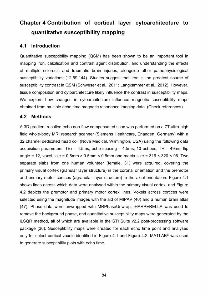
84
Chapter 4 Contribution of cortical layer cytoarchitecture to quantitative susceptibility mapping
4.1 Introduction
Quantitative susceptibility mapping (QSM) has been shown to be an important tool in
mapping iron, calcification and contrast agent distribution, and understanding the effects
of multiple sclerosis and traumatic brain injuries, alongside other pathophysiological
susceptibility variations (12,59,144). Studies suggest that iron is the greatest source of
susceptibility contrast in QSM (Schweser et al., 2011; Langkammer et al., 2012). However,
tissue composition and cytoarchitecture likely influence the contrast in susceptibility maps.
We explore how changes in cytoarchitecture influence magnetic susceptibility maps
obtained from multiple echo time magnetic resonance imaging data. (Check references).
4.2 Methods
A 3D gradient recalled echo non-flow compensated scan was performed on a 7T ultra-high
field whole-body MRI research scanner (Siemens Healthcare, Erlangen, Germany) with a
32 channel dedicated head coil (Nova Medical, Wilmington, USA) using the following data
acquisition parameters: TE1 = 4.5ms, echo spacing = 4.5ms, 10 echoes, TR = 49ms, flip
angle = 12, voxel size = 0.5mm × 0.5mm × 0.5mm and matrix size = 316 × 320 × 96. Two
separate slabs from one human volunteer (female, 31) were acquired, covering the
primary visual cortex (granular layer structure) in the coronal orientation and the premotor
and primary motor cortices (agranular layer structure) in the axial orientation. Figure 4.1
shows lines across which data were analysed within the primary visual cortex, and Figure
4.2 depicts the premotor and primary motor cortex lines. Voxels across cortices were
selected using the magnitude images with the aid of MIPAV (46) and a human brain atlas
(47). Phase data were unwrapped with MRPhaseUnwrap, iHARPERELLA was used to
remove the background phase, and quantitative susceptibility maps were generated by the
iLSQR method, all of which are available in the STI Suite v2.2 post-processing software
package (30). Susceptibility maps were created for each echo time point and analysed
only for select cortical voxels identified in Figure 4.1 and Figure 4.2. MATLAB® was used
to generate susceptibility plots with echo time.

85
4.3 Results
Figure 4.3 shows the susceptibility plots across echo times for the series of voxels
selected along the line of gennari, and just above and just below the line of gennari. The
line of gennari is layer 4B and it is known to contain highly myelinated axons (110). The
dissimilarity in the curves likely indicates different myeloarchitecture across different layers
of the cortex. In Figure 4.4 the cortical structure is assessed. Figure 4.4 (I-III) are
susceptibility plots perpendicular to the cortex, whereas Figure 4.4(IV-VI) are plots along
the cortex. Moreover, Figure 4.4(I) and (IV) are for the primary visual cortex having a
granular structure (145), and the responses for the agranular cortical structure are shown
in Figure 4.4(II) and (V) for the premotor cortex and in Figure 4.4(III) and (VI) for the
primary motor cortex. For the case of the granular structure (compare Figure 4.4(I) and
(IV)), the angle between the line and the reference magnetic field of the scanner appears
to play a larger role in the susceptibility measurement than in the cortical layer, as
evidenced by the larger spread of values. However, the opposite is true for the agranular
structures (compare Figure 4.4(II) and (V) and Figure 4.4(III) and (VI)). The angle between
the reference magnetic field and cortical line taken (Figure 4.4 (I-III) appears to effect the
results in a consistent manner irrespective of whether the cortical structure is granular or
agranular. On the other hand, agranular structures have a larger influence on the
computed susceptibility than the granular structure (Figure 4.4 (IV-VI). In chapter 3, it is
observed that tissue composition and structure can influence the phase and hence
susceptibility maps. The hypothesis was to study the susceptibility maps across the line of
gennari, above and below line of gennari, as the line has a different chemical composition
than the voxels selected above and below. We expected to see different susceptibility
maps for the line of gennari as it is highly myelinated. We observed differences in
Figure 4.1 The primary visual cortex slab: (I) slab orientation, (II) cross section of the slab, (IIa) zoomed in section of the primary visual cortex and coloured lines show the voxels selected across the cortex and the white arrow identifies the line of gennari, and (IIb) blue colour shows voxels selected along the line of gennari, and red and green colours show the voxels above and below the line of gennari. Data were averaged along the red, blue and green lines after the application of the QSM pipeline.

86
susceptibility values for the line of gennari, above and below line of gennari in one
participant. This work is an accepted abstract (Surabhi Sood, Javier Urriola, Steffen
Bollmann, Markus Barth, Kieran O’Brien, David Reutens and Viktor Vegh, “Contribution of
cortical layer cytoarchitecture to quantitative susceptibility mapping”. Organization for
Human Brain Mapping, Geneva, 2016).
.
Figure 4.2 The slab cutting across the premotor and primary motor cortices: (I) slab orientation, (II) cross section of the slab, (IIa) zoomed in section showing coloured lines across selected voxels in the premotor cortex, and (IIb) zoomed in section showing coloured lines across selected voxels in the primary motor cortex. Data were averaged on either side of the top of the cortex (i.e. averaged corresponding locations of the magenta, yellow and black lines, and averaged corresponding locations of the blue, green, red and cyan lines).

87
4.4 Conclusions
Our work has demonstrated that cortical layer cytoarchitecture contributes to quantitative
susceptibility mapping. These results may help in understanding brain diseases and
disorders affecting cortical layering.
Figure 4.3 QSM plots of lines selected in the primary visual cortex, corresponding to Figure 4.1(IIa). A noticeable shift in the curves can be appreciated with a change in location.

88
Figure 4.4 Graphs showing plots from the (I, IV) primary visual cortex (granular), and (II, V) premotor and (III, VI) primary motor cortices (both agranular). In (I-III) each line corresponds to a different projection perpendicular to the cortex. In (IV-VI) voxel locations for each line are assessed. Fine lines represent individual measurements and the thick black line represents the mean of individual measurements computed at each echo time point.
89
Chapter 5 Field strength influences on gradient recalled echo MRI signal compartment frequency shifts
In Chapter 3 the susceptibility maps across echo time were studied in specific brain
regions at 7T. This Chapter is an extension to analyse the temporal effects studied in
Chapter 3. This work is performed on both 3T and 7T field strengths. Frequency is
calculated from susceptibility maps and a multi-compartment model is used to assess
frequency shifts. The Effect of field strengths on frequency shift compartments were
investigated in human brain regions.
5.1 Abstract
Different echo time dependent gradient recalled echo MRI signal trends in different brain
regions have been attributed to signal compartments in image voxels. It remains unclear
how trends in gradient recalled echo MRI signals change as a function of MRI field
strength, and how post-processing may impact signal compartments. We used two popular
quantitative susceptibility mapping methods of processing raw phase images (Laplacian
and path-based unwrapping with V-SHARP) before they were converted to frequency
shifts in six specific brain regions at 3T and 7T. The frequency shift curves varied with
echo time, and a good overlap between 3T and 7T mean frequency shift curves were
present. However, the amount of variation across participants was greater at 3T, and we
were able to obtain better compartment model fits of the signal at 7T. We also found the
temporal trends in the signal and compartment frequency shifts to change with the method
used to process images. The inter-participant averaged trends in gradient recalled echo
MRI signals were similar at 3T and 7T, and the choice of method used to process images
led to consistent results. However, the signal compartment frequency shifts obtained using
different quantitative susceptibility mapping pipelines may not be comparable.
5.2 Introduction
Gradient recalled echo magnetic resonance imaging (GRE-MRI) signals are influenced by
local variations in the magnetic field. At a scale below the size of image voxels, field
inhomogeneity can be caused by variations in tissue microstructure, orientation and
packing (130), and by the magnetic properties of tissue constituents (107). The phase of
the GRE-MRI signal is directly affected by magnetic field inhomogeneity, and can be
converted into maps of tissue phase (in radians or degrees), frequency shift (in Hz) or bulk

90
magnetic susceptibility (generally expressed in parts per billion). The latter, called
quantitative susceptibility mapping (QSM), is the preferred approach as the non-local
tissue phase is converted to a voxel value which can be interpreted directly (69). QSM has
been used to demonstrate physiological and pathological tissue characteristics such as
changes in iron levels (50,53,102) and calcification (54,146), and to measure the
distribution of contrast agents (147,148).
Studies have demonstrated that the temporal GRE-MRI signal phase is influenced by
tissue microstructure and arrangement in white matter (70,73,149). White matter signal
compartments have been defined to correspond to myelin, axonal and extracellular
spaces (80). It has thus been suggested that GRE-MRI signal compartments mapped at
the voxel level may provide important information about tissue structure, composition and
packing (150,151). However, the biological correlates of grey matter signal compartments
remain unclear. Sood et al. recently found that QSM values change as a function of echo
time in a manner that differs between brain regions (151). They were also able to explain
the non-linear relationship between GRE-MRI echo time and QSM values using signal
compartments, and suggest a link with tissue microstructure. Therefore, it seems GRE-
MRI signal compartments are not local to white matter regions, instead they appear to be
observable across the brain.
Although white matter signal compartments have been estimated at 3T (78,81), a
significant improvement in sensitivity can be achieved with the use of ultra-high field
strength (7T) scanners (11,102,112). This gain has been attributed to an increase in
induced field change due to an increase in field strength, leading to increased contrast-to-
noise ratio in phase images (11). In the presence of an external magnetic field,
microarchitectural variations of tissues create local magnetic field perturbations.
Wiggermann et al. has demonstrated a MRI frequency shift effect in multiple sclerosis, a
disease associated with changes in tissue microstructure (152). In particular, they showed
microstructural alterations in focal multiple sclerosis lesions result in MRI frequency shifts,
suggesting the presence of local field perturbations and potentially signal compartments
within image voxels. It is therefore important to understand how frequency shifts are
influenced by different tissue types, i.e. by different brain regions, and to what extent they
can be mapped using different MRI field strengths.
We decided to evaluate echo time dependent non-linear frequency shifts qualitatively
and quantitatively through signal compartmentalisation. We considered different brain
regions, namely the corpus callosum, caudate, putamen, pallidum, cerebrospinal fluid
91
(CSF) and thalamus. We performed our study at two common field strengths, 3T and 7T,
and using two popular QSM pipelines: Laplacian, an integrated method of phase
unwrapping and background field removal, and path-based unwrapping with V-SHARP
background field removal.
5.3 Methods
5.3.1 Data Acquisition
The University of Queensland human ethics committee approved this study and written
informed consent was given by six healthy participants (19, 30 and 60 year old males and
26, 33 and 47 year old females). 3D gradient recalled echo flow compensated scans were
conducted on a 7T ultra-high field whole-body MRI research scanner (Siemens
Healthcare, Erlangen, Germany) equipped with a 32 channel head coil (Nova Medical,
Wilmington, USA) using the following parameters: TE1 = 4.98ms, echo spacing = 3.13ms,
9 echoes, TR = 52ms, flip angle = 15o, voxel size = 0.75 × 0.75 × 0.75 mm, and matrix size
= 242 × 280 × 160. The same participants were scanned using a 3T Siemens Magnetom
Tim Trio scanner (Siemens Healthcare, Erlangen, Germany) using the product 32 channel
head coil with TE1 = 6.29ms, echo spacing = 5.26ms, 9 echoes, TR = 60ms, flip angle =
18o, voxel size = 1 × 1 × 1 mm, and matrix size = 210 × 210 × 120. Magnetization-
prepared rapid gradient echo (MPRAGE) has been widely used to acquire T1-weighted
anatomical images of the human brain to assess brain tissue arrangement (153). At the
ultra-high magnetic field B1 induced inhomogeneities create a bias field affecting the
image quality in MPRAGE sequence. An improved version of MPRAGE, Magnetization
Prepared 2 Rapid Acquisition Gradient Echoes (MP2RAGE) used two inversion pulses to
reduce the B1 induced inhomogeneities (89). It has been demonstrated in the study that
segmentation performed in freesurfer using MP2RAGE generated agreeable results (89).
Freesurfer is a set of software tools which is used to study cortical and subcortical
anatomy (48). Therefore, MP2RAGE data were acquired for segmentation in this study
with the following parameters: TE = 3.44ms, TR = 4550ms, TI1 = 840ms, TI2 = 2370ms,
flip angle1 = 5o, flip angle2 = 6o, voxel size = 0.75 × 0.75 × 0.75 mm, and matrix size =
300 × 320 × 256 at 7T. We used a monopolar readout for both 3T and 7T acquisitions.
Echo times for the 3T and 7T GRE-MRI data took into account the reduction in T2* at 7T
compared to 3T.

92
5.3.2 Data Processing
The 32 channel 3T GRE-MRI data were combined on the scanner as a body transmitter?
coil was used during the data acquisition. Since a 7T body coil is not available, the 32
channel 7T GRE-MRI magnitude and phase data were processed as previously described
(154). Magnitude images were used to create a mask using the brain extraction tool in FSL
(FMRIB, University of Oxford) (155). Maps of frequency shift were generated from phase
data through two different approaches: (i) A Laplacian based technique as implemented in
iHARPERELLA (129) was applied to the phase data; this is an integrated method which
performs phase unwrapping and background phase removal in a single step, and (ii)
MRPhaseUnwrap (28), a path-based phase unwrapping method was used to remove
phase wraps in the raw phase data before V-SHARP (variable radius of the spherical
kernel at the brain boundary) (41) was applied for background phase removal using the
default parameters. Magnetic susceptibility ( χ ) maps were generated using iLSQR (30) in
both cases before they were scaled to a frequency shift using 0f Bγχ∆ = , where
6 -142.577 10 HzTγ = × and 0B is the scanner field strength measured in units of Tesla. We
used the MATLAB® implementation of iHARPERELLA (HARmonic PhasE REmovaL using
the LAplacian operator), MRPhaseUnwrap, V-SHARP and iLSQR (Sparse linear and
sparse least squares) available through STI Suite (http://people.duke.edu/~cl160/). Note
that we opted to compute frequency shifts from susceptibility values by first processing raw
data using the QSM pipeline. This is in view of Wu et. al.’s recent findings, which showed
that using the QSM pipeline a more robust fitting of the signal can be achieved (90).

93
5.3.3 Regions-of-interest
3T GRE-MRI data were registered to the 7T GRE-MRI data using MIPAV (46). FreeSurfer
(156) was used to segment individual brain regions using the 7T MP2RAGE data. Six
regions-of-interest were chosen: caudate, cerebrospinal fluid (CSF), corpus callosum,
pallidum, putamen and thalamus, as shown in Figure 5.1. Regions-of-interest were eroded
(using the erode function in FSL with a threshold of 90%) to reduce partial volume effects
due to adjacent brain regions. MATLAB® (The MathWorks, Natick, MA, USA) scripts were
used to extract region-based values and to produce frequency shift plots. The first echo
time signal was subtracted from all other echo time signals for the purpose of
standardising frequency shift plots. Note that this is necessary as different systems (3T
versus 7T) have different hardware and therefore produce different phase offsets at the
first echo time.
5.3.4 GRE-MRI signal compartment fitting
We used a multi-compartment model which has independent frequency shifts for all
compartments (81):
( )*2,n
1 22
1
nbg
i f tNTi f t
nn
S t e A eπ
π
− + ∆ − ∆
=
= ∑ (6.1)
where 𝐴𝐴𝑛𝑛 are compartment contributions, 𝑇𝑇2,𝑛𝑛∗ is the signal compartment, and ∆𝑓𝑓𝑏𝑏𝑏𝑏
defines the background frequency shift for the 𝑁𝑁 compartment model. In addition to the
QSM pipeline, we used the background offset correction term (i.e. the term with ∆𝑓𝑓𝑏𝑏𝑏𝑏) to
account for any leftover background effects. Instead of presenting results for 𝐴𝐴𝑛𝑛, we
present compartment volume fractions computed by dividing each 𝐴𝐴𝑛𝑛 by the sum of 𝐴𝐴𝑛𝑛’s.
We used a previously established approach to determine the number of signal
compartments for each brain region (157). Notably, the induced change in angular
frequency is a function of the induced change in the magnetic field, as defined by the
Larmor equation ( )γ∆ = ∆f B . We converted magnetic susceptibility to frequency shifts using
0f Bγχ∆ = , where χ is the magnetic susceptibility. The Lorentzian sphere correction requires
the frequency shift to be multiplied by 1/3 (73). This change results in a linear amplification
of frequency shifts presented in the tables but does not change the relationship between
the 3T and 7T findings, nor the Laplacian and path-based results. We did not apply a
Figure 5.1 Illustration of the brain’s regions-of-interest used in this study for comparing temporal frequency
shift curves. These are also the regions for which signal compartmentalisation was performed.

94
correction as it is unclear whether this correction is widely applicable across different brain
regions.
To assist convergence to an optimal solution using the approach described by Nam et
al. (81), we up-sampled our nine echo point complex signal to 17 echo time points (i.e.
inserted one echo time point between all measurements) using the interp1 function in
MATLAB®. Since the frequency shift evolves smoothly as a function of echo time, we may
assume values are continuous and additional points can be added. We found up-sampling
to help with convergence towards a solution. Nam et al. (81) computed myelin water
fraction maps using 16, 24 and 32 echo time points, and found 16 echo time points were
able to produce consistent fitting as measured by parameter variations. For each
segmented brain region we fitted the complex signal as a function of echo time after
averaging data in a single region across participants. We computed the standard error of
regression (SER) as a measure of the quality of fit; a value of < 10% indicates a very good
level of fit and values > 20% indicate a poor fit.
We repeated the 3T GRE-MRI data fitting when frequency shifts were fixed to those
obtained using the 7T data and scaled using the field strength ratio (i.e. 3/7). Thereby, we
provide compartment frequency shift results at 3T (Δf3T) at 7T (Δf7T) and corresponding
volume fractions (VF3T and VF7T), and volume fractions when 3T frequency shifts were
fixed based on 7T values (VFfixed). Additionally, we computed the Fréchet distance
between mean curves to establish how close values are between 3T and 7T
measurements, and to be able to comment on how methodological differences can impact
on the curves. The Fréchet distance takes into account the location and ordering of the
points, making it a suitable measure for our study.
5.4 Results
5.4.1 Frequency shifts as a function of echo time
Figure 5.2 depicts frequency shift curves for each of the six brain regions investigated
using the Laplacian method at the 3T and 7T field strengths. Frequency shifts have been
plotted as a function of echo point. The solid line in each plot corresponds to the mean
frequency shift after averaging voxel values in each region and across participants. The
shaded area matched in colour with the solid line shows the inter-participant variation via
one standard deviation from the mean. Similarly, Figure 5.3 provides results obtained
using the path-based method.

95
Based on results presented in Figure 5.2 and Figure 5.3, three main points can be made.
First, irrespective of the method, a good level of correspondence between 3T and 7T
curves is present. Second, the 3T mean curves have a tendency to oscillate as a function
of echo point more than the 7T curves. Third, the inter-participant variation is larger at 3T
than at 7T. In Table 5.1 a summary of the area spanned by each shaded region in Figure
5.2 and 5.3 is provided. We may note that at 7T the level of inter-participant variation is
approximately halved.
Interestingly, the ordering of the Fréchet distances is comparable between the Laplacian
and path-based methods, suggesting that a fair level of intra-method consistency is
present. In Table 5.2 the Fréchet distance between 3T and 7T curves has been tabulated.
Fréchet distance can be defined as a measure of similarity between the curves. A value
closer to zero implies curves are more similar, whilst larger values suggest less similarity
between curves. However, it should not be confused with only points close to both data
sets. This means the location and ordering of the points are also taken into account. In
other words the fluctuation of data is important. For example, in the corpus callosum for
the Laplacian method, there are two sharp fluctuations at 6th and 8th echoes, whereas in
the path-based method there is no sharp fluctuation. Hence, the Fréchet distances are
7.8ppb and 5.5ppb for the Laplacian and the path-based respectively in the corpus
callosum. Similarly, in CSF there are two major fluctuations observed at the 4th and 6th
echoes for the Laplacian, and no major fluctuation is observed in the path based method.
Thus, the Fréchet distance in the Laplacian is higher than in the path-based method. In the
putamen using the Laplacian method the fluctuation is twice upwards and twice
downwards, which is why despite the curves in the Laplacian being very close, the
Fréchet distance is much higher in the Laplacian, 2.5ppb, as compared to the path-based,
0.9ppb. The Fréchet distance for the caudate is 1.5ppb for the Laplacian and 1.6ppb for
the path-based. It should be noted here that there is no fluctuation or similar shape curves.
Additionally, for the thalamus the fluctuation and shape curve is similar, and hence the
Fréchet distance is similar. In the pallidum, for the Laplacian method there are minor
fluctuations on echoes 2, 5, 6 , 7, and 8 with a change in the shape of the curve, whereas
for the path-based there are minor fluctuations at the 2nd ,4th , and 6th echoes, therefore
explaining the Fréchet distance values.
5.4.2 Signal compartmentalisation
Table 5.3 provides the three compartment fitting results based on the data generated
using the Laplacian method. Similarly, Table 5.4 was generated using the path-based

96
data. Model parameters were obtained by fitting the 3T and 7T multi-echo data, and
frequency shifts have been presented alongside the standard error of regression (i.e.
SERM and SERP calculated based on the signal magnitude and phase, respectively). We
found either two (the putamen, pallidum, CSF and thalamus) or three (the corpus callosum
and caudate) signal compartments. Irrespective of whether the Laplacian or path-based
method was used to generate the data, the number of compartments for a specific region
were the same. Moreover, the 7T data was able to be better fitted than the 3T data (i.e.
SERM and SERP at 7T was less than at 3T). Frequency shifts have been arranged by the
size of the compartment volume fractions, that is from largest to smallest. We should point
out that since we used the model which incorporates the background offset term (see
Equation (5.1)), the presented frequency shifts may be shifted with respect to each other.
In addition, we did not reference frequency shifts with respect to a particular compartment.
For this reason, it is more important to focus on the separation between frequency shifts
than their actual value.
For the corpus callosum, using the Laplacian data, a good level of fit (SER < 10%) was
achieved for all three cases (i.e. 7T, 3T and 3T fixed with 7T frequency shifts). The
compartment frequency shifts were also similar, suggesting that three compartments can
be resolved at both 3T and 7T and the level of variation in frequency shifts between 3T
and 7T is too small to cause a large error in the fit when 7T frequency shifts are used to fit
3T data (SERM = 6.9% and SERP = 8.4%). Hence, the ability to fit the 3T curve does not
deteriorate with the difference between 3T and 7T shifts. Whilst the volume fractions
changed somewhat between 3T and 7T fits, the volume fraction estimated from the 7T
data was recoverable from the 3T data using 7T frequency shifts (compare volume
fractions of 44.7% to 43.0%, 36.1% to 38.3% and 19.2% to 18.7%). The path-based
results showed a similar trend in compartment values, however the volume fractions were
less recoverable based on 3T data.
In the caudate using two compartments and the Laplacian data, we were not able to
obtain a good fit. With the use of the three compartment model, we did achieve low SER
values and we found a third compartment with a high frequency shift and low volume
fraction. The frequency shift obtained using the 7T data was able to better explain the
trends in the 3T data (compare SERM = 0.7% and SERP = 9.8% to SERM = 0.9% and
SERP = 8.5%). Based on the path-based data, the fit did not improve when 3T frequency
shifts were set based on those generated from the 7T data. Otherwise, the overall trends
were similar.
97
For the putamen the Laplacian-based frequency shifts had a larger separation than
those generated from the path-based data. The negative frequency shift in both cases had
a larger volume fraction than the positive shift, and the fit at 3T decreased when fixed 7T
frequency shifts were applied. The trends in the compartment values for the pallidum were
similar to those obtained for the putamen. However, the fit for the pallidum was worse than
that for the putamen (SERP > 10% in the pallidum versus SERP < 10% in the putamen, not
including the fixed result). The thalamus also had two compartments with a negative and
positive frequency shift and the negative frequency shift compartment had a larger volume
fraction. The frequency shift separation between compartments is similar between the
putamen and pallidum (around 40ppb for the Laplacian and around 30ppb for the path-
based), which increases in the thalamus (around 50ppb for both Laplacian and path-
based).
In the CSF a dominant compartment (around 80%) was found with a frequency shift of
around -20ppb irrespective of whether the Laplacian or path-based data were used in the
fitting. The 7T data resulted in a larger frequency shift for the smaller volume fraction
compartment in comparison to what was estimated based on 3T data. Whilst the fit
deteriorated with the fixing of frequency shifts for the 3T fitting, the fitting quality was still
comparable.

98
Figure 5.2 Frequency shifts as a function of the echo point in the six brain regions obtained using the
Laplacian reconstruction pipeline. Solid lines are the averaged values obtained for the brain region based on
all participants, and the standard deviation of values is shown with the corresponding colour shaded region corresponding to inter-participant variability.

99
Figure 5.3 Frequency shift values as a function of the echo point in the six brain regions obtained using the path-based reconstruction pipeline. Plot description as per Figure 5.2.

100
Region Laplace Path-based
3T 7T 3T 7T
Corpus callosum 418 176 292 210
Caudate 351 147 183 90
Putamen 173 72 146 60
Pallidum 251 123 286 122
CSF 212 117 196 91
Thalamus 178 100 189 114
Region Laplace (3T-7T) Path-based (3T-7T)
Corpus callosum 7.8 5.5
Caudate 1.5 1.6
Putamen 2.5 0.9
Pallidum 5.1 2.2
CSF 2.7 1.2
Thalamus 2.6 2.6
Table 5.1 Areas (in units of ppb۰ms) spanned by the variations shown in Figure 5.2 and 5.3, calculated by taking the difference between the upper and lower error bounds at each echo point and by summing over echo numbers. The variation reduces with increase in the field strength, suggesting that inter-participant variability can be mitigated through field strength increases.
Table 5.2 Fréchet distance (in ppb) calculated between 3T and 7T mean curves for the six brain regions
based on both Laplace and path-based reconstruction methods. A value of zero implies curves completely
overlap, whilst increasingly larger values reflect increasingly larger distances between curves.
Table 5.3 Signal compartment parameters computed based on the Laplacian data. This table summarises
Δf7T and Δf3T values which denote 7T and 3T freqeuncy shifts for each of the signal compartments.
Depending on the region, either two or three columns are shown corresponding to two or three signal
compartments for that brain region. Respective volume fractions, VF7T and VF3T have been tabulated as well.
VFfixed refers to volume fractions when 7T frequency shifts were used to fit 3T data. The standard error of
regression (SER) was calculated based on signal magnitude (M) and phase (P).

101
Laplacian
Corp
us c
allo
sum
∆𝒇𝒇7T (ppb) -77.9 59.6 16.7
SERM (%)
SERP (%) ∆𝒇𝒇3T (ppb) -65.6 34.1 5.5
VF7T (%) 44.7 36.1 19.2 7.5 4.1
VF3T (%) 57.3 24.4 18.3 9.1 5.9
VFfixed (%) 43.0 38.3 18.7 6.9 8.4
Caud
ate
∆𝒇𝒇7T (ppb) 7.3 -45.5 106.8
SERM (%)
SERP (%) ∆𝒇𝒇3T (ppb) 3.1 -69.0 143.7
VF7T (%) 64.3 29.2 6.5 0.3 6.3
VF3T (%) 74.2 16.6 9.2 0.7 9.8
VFfixed (%) 66.8 31.2 2.0 0.9 8.5
Puta
men
∆𝒇𝒇7T (ppb) -19.4 19.0
SERM (%)
SERP (%) ∆𝒇𝒇3T (ppb) -19.7 29.8
VF7T (%) 61.6 38.4 0.9 5.1
VF3T (%) 58.8 41.2 1.1 7.5
VFfixed (%) 59.4 40.6 1.5 12.6
Palli
dum
∆𝒇𝒇7T (ppb) -18.4 21.4
SERM (%)
SERP (%) ∆𝒇𝒇3T (ppb) -25.5 16.6
VF7T (%) 78.5 21.5 0.8 13.6
VF3T (%) 66.4 33.6 1.8 16.9
VFfixed (%) 68.8 31.2 1.7 18.6
CSF
∆𝒇𝒇7T (ppb) -15.2 107.0
SERM (%)
SERP (%) ∆𝒇𝒇3T (ppb) -21.5 47.1
VF7T (%) 79.7 20.3 2.0 4.6
VF3T (%) 79.9 20.1 4.3 6.7
VFfixed (%) 84.9 15.1 3.7 8.8
Thal
amus
∆𝒇𝒇7T (ppb) -15.6 37.0
SERM (%)
SERP (%) ∆𝒇𝒇3T (ppb) -25.9 16.0
VF7T (%) 72.6 27.4 0.7 5.7
VF3T (%) 55.3 44.7 0.9 8.4
VFfixed (%) 70.9 29.1 0.8 9.1

102
Path-based Co
rpus
cal
losu
m
∆𝒇𝒇7T (ppb) -60.3 65.8 20.4
SERM (%)
SERP (%) ∆𝒇𝒇3T (ppb) -44.5 55.7 18.3
VF7T (%) 51.4 30.6 18.0 4.8 3.9
VF3T (%) 69.5 21.3 9.2 6.1 5.9
VFfixed (%) 58.2 21.4 12.4 5.9 6.9
Caud
ate
∆𝒇𝒇7T (ppb) 9.6 -37.2 113.3
SERM (%)
SERP (%) ∆𝒇𝒇3T (ppb) 6.1 -62.9 165.8
VF7T (%) 62.1 30.3 7.6 0.2 2.2
VF3T (%) 79.2 16.5 4.3 0.2 6.1
VFfixed (%) 53.2 36.4 10.4 0.3 8.4
Puta
men
∆𝒇𝒇7T (ppb) -13.7 13.5
SERM (%)
SERP (%) ∆𝒇𝒇3T (ppb) -12.0 28.8
VF7T (%) 74.8 25.2 0.6 5.5
VF3T (%) 81.1 18.9 1.8 8.6
VFfixed (%) 66.3 33.7 1.7 11.1
Palli
dum
∆𝒇𝒇7T (ppb) -17.6 18.3
SERM (%)
SERP (%) ∆𝒇𝒇3T (ppb) -85.0 6.8
VF7T (%) 90.5 9.5 2.0 15.7
VF3T (%) 87.3 12.7 4.7 19.9
VFfixed (%) 71.2 28.8 1.7 16.3
CSF
∆𝒇𝒇7T (ppb) -22.2 98.0
SERM (%)
SERP (%) ∆𝒇𝒇3T (ppb) -30.7 53.5
VF7T (%) 80.0 20.0 2.2 4.6
VF3T (%) 75.8 24.2 3.0 6.6
VFfixed (%) 89.5 10.5 3.3 4.7
Thal
a
mus
∆𝒇𝒇7T (ppb) -12.6 40.5
SERM (%)
SERP (%) ∆𝒇𝒇3T (ppb) -7.9 50.3
Table 5.4 Signal compartment parameters computed based on the path-based data. Description of entries
as per Table 5.3.

103
VF7T (%) 77.1 22.9 0.2 5.9
VF3T (%) 96.1 3.9 0.6 9.3
VFfixed (%) 88.2 11.8 0.9 10.0
5.5 Discussion
We studied echo time dependent non-linear frequency shifts in six human brain regions
(corpus callosum, caudate, putamen, pallidum, CSF and thalamus). Frequency shifts were
generated after data were processed using two different QSM pipelines. Our results
suggest four key findings. Firstly, the temporal trend in frequency shift as a function of
echo time varied across brain regions and the trend was observed at 7T and 3T. Secondly,
frequency shifts computed from 7T GRE-MRI data had less variability than those obtained
using 3T data. This is expected because the signal-to-noise ratio increases with scanner
field strength. Thirdly, we found the compartment fitting was generally better at 7T as
opposed to 3T. Finally, compartments can be found irrespective of the field strength and
processing method used.
5.5.1 Previous findings on echo time dependence
Using GRE-MRI data, the frequency shift in white matter voxels varies as a function of
echo time. It has been suggested that this reflects the influence of fibre orientation with
respect to the scanner field on temporal signal formation (69). In a previous study that
simulated the expected frequency shifts as a function of echo time for different white
matter orientations with respect to the scanner field (80), the largest effect was observed
when the fibre orientation was perpendicular to the scanner field. We segmented the
corpus callosum near the mid-sagittal plane where fibre orientation is expected to be
approximately perpendicular to the scanner field. The trend in the frequency shift curve is
present and the overlap between 3T and 7T findings is suggestive of compartmental
influences on 3T and 7T GRE-MRI signals.
Studies have confirmed a non-linear relationship between the GRE-MRI phase signal
and echo time (90,130,151). GRE-MRI data could provide information about the
microstructure of the tissue in white matter by characterizing myelin, axonal and
extracellular compartments on T2* values (78). We recently showed echo time
dependence of frequency shifts and observed different patterns in different brain structures
including the corpus callosum, caudate, internal capsule, fornix, thalamus, putamen,
pallidum, insula, red nucleus and substantia nigra (151). Others have observed a non-
104
linear phase accumulation in the GRE-MRI signal (91). This contributes to temporal
susceptibility trends since susceptibility is derived from phase.
5.5.2 Signal compartments
Echo time dependence has been explained in terms of signal compartmentalisation
(69,78,80). These studies suggest the presence of multiple voxel constituents, which
additively contribute to the complex voxel signal. Whilst myelin and iron have been
identified as the largest contributors to variations in susceptibility, it has also been
suggested that other microscopic contributions, such as packing and organisation, could
affect frequency shift temporally (158).
We used two and three compartment signal models based on previously established
model selection criteria to assess quantitative differences between brain regions. The
signal compartments obtained using the 7T data were able to explain echo time
dependence in specific regions at 3T, suggesting that distinct frequency shifts influence
temporal GRE-MRI signal formation in specific brain regions. For the corpus callosum and
the caudate, three compartments provided a better fit, whereas for the putamen, pallidum,
CSF and thalamus, two compartment signal models fit the data. This was observed
irrespective of whether the Laplacian or path-based method was used.
For the corpus callosum three distinct frequency shift compartments corresponding to
axonal and extracellular water and myelin have been defined in the literature (85). Note
that previous findings have reported myelin T2* values or around 10ms, and myelin has
been shown to have the shortest T2*. Based on this value, we would expect a 53% myelin
signal to be present at 6.29ms (first echo at 3T), 37% at 10ms and 14% at 20ms. Hence,
the shortest T2* compartment should contribute to at least the first four echo points, which
when up sampled, leads to contributions to 7 out of the 17 echo points.
White matter regions and their compartments have been studied in three separate 7T
experiments and they all used a different compartment as reference. This precludes a
direct comparison of values, but it is still possible to compare the frequency shift difference
between compartments. Van Gelderen et al. found compartment frequency shift
separations of 35.8Hz and 7.0Hz in the splenium of the corpus callosum and 31.8Hz and
5.9Hz in the posterior internal capsule (78). Sati et al.’s results have frequency shift
separations of 35.9Hz and 6.1Hz (80), and Li et al. found 32.1Hz and 6.3Hz (85). At 7T the
Laplacian method yielded separations of 28.2Hz (94.6ppb) and 12.8Hz (42.9ppb) and the
path-based result produced separations of 24.0Hz (80.7ppb) and 13.5Hz (45.4ppb).

105
Thapaliya et al. investigated how frequency shifts across the mid-sagittal plane of the
corpus callosum vary and found compartmental separations between 15Hz and 35Hz with
a mean of around 25Hz, and -7Hz to -13Hz with a mean around -9Hz (159). The difference
between our results and those previously published probably relates to differences in the
white matter region assessed, and potentially to the compartment model. We segmented
the corpus callosum between the genu and the splenium with a limited sagittal thickness
(about 4mm), and it has been shown that compartment values can vary across the mid-
sagittal plane of the corpus callosum (159). Thapaliya et al. and this work used the same
compartment model, i.e. one with background offset correction, whereas others did not
use a term for background offset correction. The 3T and 7T Laplacian and path-based
results were consistent, as implied by the fit when frequency shifts at 3T were fixed
according to 7T frequency shifts (taking into account differences in field strength).
Duyn et al. has demonstrated that field strength influences the visualization of
anatomical details (11). Furthermore, it was shown that phase data contains intricate
details which were not present in the magnitude information. Therefore, we decided to
study the influence of field strength on the multi-compartmental model in different brain
regions in six participants. We also planned to investigate frequency shift compartments
using different methods. We expected to see better sensitivity at 7T and we observed a
higher sensitivity at a higher field strength. We also observed that similar compartments
that we found at both 3T and 7T. Methodological differences were also found to influence
compartments.
5.6 Conclusion
We investigated frequency shifts as a function of echo time in six human brain regions
using 3T and 7T GRE-MRI data, and by applying different methods (Laplacian and path-
based) in the QSM pipeline. We performed signal compartmentalisation to quantitatively
characterise changes due to variations in the scanner field strength. In general, we found
the compartment model to better fit the 7T data than the 3T data. We also found a good
agreement between 3T and 7T compartment frequency shifts. Our results suggest that the
method used to process the data can influence compartment frequency shifts, however
consistent results can be generated using either method investigated. Signal
compartmentalisation may lead to the identification of important biomarkers of brain
diseases provided a consistent processing pipeline is used.

106

107
Chapter 6 Evaluation of multi-echo QSM in the brain cortex using ultra-high field
We have advanced the GRE-MRI signal compartments to the human cerebral cortex in
this chapter. As orientation is an important aspect in QSM pipeline, the effect of orientation
is also explored in the chosen Brodmann areas.
6.1 Abstract
The cerebral cortex is formed of different cyto/myelo-architectural regions and, gradient
recalled echo MRI data has been shown to be sensitive to tissue differences at the
microscale. The potential use of multi-echo gradient recalled echo MRI data for cortical
parcellation and the relationship between the derived frequency shift and cortical region
has not been established. Multi-echo gradient recalled echo measurements were
performed on a 7T MRI scanner. Four Brodmann areas were considered: BA6 (premotor
cortex), BA4 (primary motor cortex), BAV1 (primary visual cortex) and BAV2 (secondary
visual cortex). For each region and in six participants, frequency shift curves were
generated using a multi-orientation quantitative susceptibility mapping method (i.e. TKD)
and a single orientation quantitative susceptibility mapping method (i.e. iLSQR). The
Fréchet distance between echo-time dependent frequency shift curves was measured
across cortical regions, and curves were also parameterised using a multi-compartment
signal model. We found echo time dependent frequency shift curves to differ between
Brodmann areas when both multi- and single orientation reconstruction methods were
used to generate curves. The frequency shift parameter of the signal model differentiated
between cortical regions clearly. Our inter and intra-participant analyses suggest the
potential of parcellating the human cerebral cortex using frequency shift based
measurements derived from multi-echo gradient recalled echo MRI data.
6.2 Introduction
Gradient recalled echo (GRE)-MRI data forms the basis of quantitation of tissue T2* and
magnetic susceptibility values. Whilst the former is generated from GRE-MRI magnitude
images, the latter relies on corresponding phase images. With the increased availability of
ultra-high field MRI scanners (i.e. 7T and above), ultra-high field MRI studies have focused
on the evaluation of differences between magnitude and phase images. It has now been

108
established that 7T MRI phase images can delineate anatomical structures with superior
image contrast to magnitude images (11,25). The exquisite phase image contrast
achieved at 7T has been attributed to tissue composition and architecture in relation to
proteins, lipids, non-heme tissue iron, and deoxyhemoglobin at cellular and subcellular
levels (73). These tissue specific MRI image voxel inclusions have been associated with
microscale spatial variations in magnetic susceptibility, which perturb the MRI scanner
field. As GRE-MRI data is highly influenced by magnetic field effects, information on tissue
microstructure and composition is reflected in the voxel signal (69,87,130,150).
Since biological tissue is highly heterogeneous, and different tissues can have different
packing and organisation of microstructural components, the orientation of the magnetic
field of the scanner with respect to tissue orientation/structure induces an orientation
specific change in the field. This has been confirmed through a demonstration of tissue
orientation dependence in GRE-MRI data (69). As such, quantitative susceptibility
mapping (QSM) methods using multiple (e.g. COSMOS (147); TKD (62)) and single
orientation (e.g. iLSQR (30), PDF (38), MEDI (50)) data have been developed. To date,
multiple orientation methods form the standard in terms of mapping tissue susceptibility at
a single echo time as they demonstrate the least dependence on the orientation of the field
with respect to the tissue.
The calculation of susceptibility maps through multiple orientation sampling (COSMOS)
requires data to be acquired with a minimum of three orientations with 60o differences
between rotations (147), and many more with head rotations with angles around 10o.
Therefore, COSMOS is impractical for head imaging applications as data acquisition times
become unreasonably long. Threshold-based k-space division (TKD), a method which can
use as few as two or three head rotations, was developed to overcome scanning
limitations associated with COSMOS (62). Whilst TKD does not perform as well as
COSMOS, it provides an intermediate between single orientation methods and COSMOS.
With single orientation QSM methods the biggest challenge is to address the ill-posed
inverse problem associated with computing a magnetic susceptibility from measured field
perturbations. The ill-posedness associated with missing data (i.e. under sampling) at the
magic angle of 54.7o results in streaking artefacts in reconstructed susceptibility maps.
New reconstruction methods which use regularisation, and magnitude image and tissue
priors in the QSM pipeline have been developed to reduce streaking artefacts (40,50,54).
Whilst a number of single orientation methods are able to produce comparable results, the
iterative sparse linear and sparse least squares (iLSQR) method was shown to be robust

109
(90), and it is routinely used in neuroimaging studies. We should note that multiple
orientation methods inherently oversample, and methods to correct for streaking artefacts
are not needed.
Studies have also investigated the information contained in multiple echo time GRE-
MRI data. It has been proposed that temporal information potentially reflects the
underlying tissue arrangement or composition (87). Several modelling techniques have
been implemented to parameterise the sub-voxel susceptibility effects in white matter
(78,80,85) and grey matter (87). Multi-compartment GRE-MRI signal modelling has been
investigated as a tool to parameterise the variations in tissue microstructure (87,160,161),
and specific model parameters may directly link with distinct biological features of complex
tissues (157). Recently, it was shown that the frequency shift parameter derived from the
GRE-MRI signal model is likely to be informative about tissue composition (132,157).
A major challenge in neuroscience is the parcellation of the cerebral cortex within
individuals into different cyto43myelo-architectural regions (162). Based on existing
findings on the influences on the multiple echo GRE-MRI signal, we decided to evaluate
the utility of multiple echo time GRE-MRI data in differentiating between Brodmann areas
using temporal frequency shift curves generated using multiple (i.e. TKD) and single (i.e.
iLSQR) orientation quantitative susceptibility mapping pipelines. We also sought to
establish how the frequency shift parameter generated using an existing multiple echo
time GRE-MRI signal compartment model varies across specific Brodmann areas.
6.3 Materials and Methods
6.3.1 MRI data acquisition
Imaging protocols were approved by University of Queensland human ethics committee
and informed written consent was obtained from six female participants aged 31, 30, 31,
36, 36, and 34. The ages were chosen based on the brain maturing by the age of 27 (163),
and females in general have thicker cortices than males with a higher number of voxels in
each region (164). A homogeneous cohort was chosen for a cortical study as the cortical
thickness varies with gender and age. Measurements were made with a non-flow
compensated 3D 𝑇𝑇2∗-weighted gradient recalled echo (GRE) sequence on a 7T ultra-high
field whole-body MRI research scanner (Siemens Healthcare, Erlangen, Germany) with a
32 channel dedicated head coil (Nova Medical, Wilmington, USA). A 𝑇𝑇1-weighted
MP2RAGE sequence was also acquired for the same participants with the following
parameters: TE1 = 3.44ms, TR = 4.3s, voxel size = 0.75mm × 0.75mm × 0.75mm, TI1 =

110
840ms, TI2 = 2.37s, α1 = 5o, α2 = 6o, matrix size = 300 × 320 × 256, bandwidth 250 Hz/Px,
acquisition time = 6m 54s, and PAT mode = GRAPPA, acceleration factor = 3. We used
monopolar readouts for 7T acquisitions.
GRE-MRI data for two different fieldsofview (i.e. slabs across the brain in axial and
coronal orientation) were acquired, as in Figure 6.1. The acquisition parameters were: TE1
= 4.5ms, echo spacing = 4.5ms, 10 echoes, TR = 49ms, α = 12, voxel size =
0.5mm × 0.5mm × 0.5mm, matrix size = 316 × 320 × 96, bandwidth 620 Hz/Px, acquisition
time = 9m 50s, and parallel acquisition techniques (PAT) mode = Generalized
autocalibrating partial parallel acquisition (GRAPPA), acceleration factor = 2. For each
slab, data were acquired four times: two normal (normal1 and normal2), one backward and
one forward tilts of the head. We aimed to achieve the maximum comfortable head
rotations (~ 10o) with respect to the normal orientation. Padded neck and head supports
were used to keep the head held in position in each orientation. Scanner generated data
were stored as the magnitude and phase images for each channel, and converted to NIfTI
format via MATLAB® (The MathWorks, Inc., Natick, Massachusetts, United States) scripts.
6.3.2 Single orientation susceptibility mapping
The MP2RAGE dataset was used to segment the brain using Freesurfer. The MP2RAGE
sequence was used as a good quality T1-weighted image is required for processing
procedures in Freesurfer (156). T1-weighted MPRAGE or MP2RAGE can be used for
Freesurfer segmentation, however a better GM/WM contrast is observed in MP2RAGE as
compared to MPRAGE which is important for segmentation (165). MP2RAGE acquires
data rapidly at two points during inversion recovery, and then it combines two volumes to
cancel bias fields, therefore making it useful at an ultra-high field strength (7T).
For cortical reconstruction recon-all command is used in Freesurfer. There are several
steps involved in the reconstruction using recon-all. With the recon-all command, all
reconstruction can be performed in one step or step-wise processing can be done. The
steps involved in recon-all are: Motion Correction, NU (Non-Uniform) Intensity Correction,
Talairach, Normalization, Skull Strip, Automatic Subcortical Segmentation, EM(GCA)
Registration, CA Normalize, CA Register, Remove Neck, EM Registration, with skull, CA
label, Aseg stats, Normalization2, WM segmentation, Cut/Fill, Tessellation, Orig Surface
Smoothing, Inflation, QSphere, Automatic Topology Fixer, Final Surfaces, Cortical Ribbon
Mask, Spherical Inflation, Ipsilateral Surface Registration, Contralateral Surface
Registration, Average Curvature, Cortical Parcellation, and Parcellation Statistics.

111
MP2RAGE data at 7T can cause a bias field and hence Talairach failures. The Talairach
processing steps are therefore not useful and the directive -notal-check can be used to
remove Talairach processing. Another method is to use the bias field correction at 7T
(166).
To create susceptibility maps, phase data were first background phase corrected then
converted to susceptibility maps. Magnetic susceptibility ( χ ) maps were generated using
iLSQR (30) before they were scaled to a frequency shift using 0f Bγχ∆ = , where
6 -142.577 10 HzTγ = × and 0B is the scanner field strength measured in units of Tesla. Note
that we opted to compute frequency shifts from susceptibility values by first processing raw
data using the QSM pipeline. This is in view of Wu et. al.’s recent findings that by using the
QSM pipeline a more robust fitting of the signal can be achieved (90). Background phases
were removed using the iHARPERELLA (i.e. Harmonic phase removal using the Laplacian
operator) method (7), and susceptibility maps were generated using the iLSQR method
(61). The STI Suite version 2 implementations of iHARPERELLA and iLSQR were used
(30). Data from each channel was processed separately and susceptibility maps were
combined using selective combine (167,168). Selective combination of channel data has
been shown to lead to high quality data. The approach was applied to data from each slab
in each orientation.
6.3.3 Multiple orientation susceptibility mapping
Susceptibility maps were also computed using TKD with three different thresholds: 0.06,
0.12 (default) and 0.24 (62). The first echo time susceptibility maps of normal2, backward
and forward orientations in each slab and for each participant were registered onto
normal1 orientation using MIPAV (46). The registration matrix was applied to all other echo
time susceptibility maps. Susceptibility maps (in ppm) were converted to frequency shift
maps (in Hz) at each echo time by multiplying susceptibility images by γB0, where γ =
42.577MHzT-1 and B0 = 7T in our study. The mapping of frequency shift images from
susceptibility maps instead of the mapping of frequency shifts directly from background
phase corrected phase images was justified recently (90). To address method related
baseline differences in phase offsets, the first echo time frequency shift image was
subtracted from each subsequent echo time frequency shift image using MATLAB®.

112
6.3.4 Cortical areas
Four different Brodmann Areas (BA) were chosen based on their microstructural
differences. The premotor cortex (BA6) and primary motor cortex (BA4) are agranular
brain regions, whereas the primary visual cortex (BAV1) and secondary visual cortex
(BAV2) are granular brain regions. Whilst granular regions have a well-developed layer IV,
agranular regions do not develop this layer. Brain regions were segmented using the
Brodmann labels available in Freesurfer (156). Figure 6.2 shows the extent of these
regions throughout the brain. The FreeSurfer Brodmann labels were converted into
volumetric regions-of-interest (ROIs) and transformed to the native MP2RAGE space
using mrilabel2vol. Each region was eroded to reduce any partial volume effects, and then
binarised to form a region mask. The ROIs (obtained after mrilabel2vol) in MP2RAGE
space were then registered onto the normal1 GRE space data using MIPAV (46). For the
purpose of presenting the results, a weighted mean frequency shift value across
participants was computed (since the number of image voxels in a specific region varied
Figure 6.1 Illustration of the Brodmann areas (i.e. regions-of-interest) and orientations of the two slabs with
respect to the scanner field, B0. In (a) cortical regions BA6, BA4, BAV1 and BAV2 are shown over an inflated
brain surface, (b) middle slice of the slab acquired in the axial orientation covering the primary motor cortex,
BA4, and premotor cortex, BA6. Similarly, in (c) the middle slice of the coronal slab used for data acquisition,
covering the primary visual cortex, BAV1, and secondary visual cortex, BAV2, is shown.

113
across participants) and standard deviations were pooled across participants. Differences
between temporal frequency shift curves were established using the Fréchet distance
(169,170). The Fréchet distance is based on the location and ordering of the points of two
curves. A value closer to zero suggests curves to be more similar, whereas large Fréchet
distances imply deviation of curves.
6.3.5 GRE-MRI signal compartment fitting
Parameterisation of echo time dependent signals (S) was performed using an existing
multi-compartment model (171):
( )*2,n
1 22
1,
n Ebg E
i f tNTi f t
E nn
S t e A eπ
π
− + ∆ − ∆
=
= ∑ (6.2)
where tE is echo time, and 𝐴𝐴𝑛𝑛 are water fractions, 𝑇𝑇2,𝑛𝑛∗ are relaxation times and ∆𝑓𝑓𝑛𝑛 are
frequency shifts associated with each compartment. Here, residual background effects not
removed using the susceptibility pipeline are accounted for by ∆𝑓𝑓𝑏𝑏𝑏𝑏 and 𝑁𝑁 defines the
number of signal compartments in the model. Values of 𝐴𝐴𝑛𝑛 are presented as a fraction of
the total signal. The computed frequency shifts were multiplied 1/3, which is the Lorentzian
Figure 6.2 ROIs (premotor cortex BA6, primary motor cortex BA4, primary visual cortex BAV1, and
secondary visual cortex BAV2) shown on different slices in (a) coronal, (b) axial, and (c) sagittal orientation.

114
sphere correction (73). We resampled our 10 echo point data to 19 echo points using the
interp1 function in MATLAB®, simply to aid the convergence rate of the lsqnonlin
optimisation algorithm also in MATLAB®. Differentiability of the data collected can be
assumed at any echo point collected, since magnitude and frequency shifts evolve
smoothly as a function of echo time. Nam et al. computed 𝐴𝐴𝑛𝑛’s based on data with 16, 24
and 32 echo points, and found 16 echo points to be adequate for a three (i.e. N = 3)
compartment model (81).
6.4 Results
An example of the ten echo point GRE-MRI data collected within each of the two slabs are
depicted in Figure 6.3. Any residual phase errors in the cortex were corrected by
calculating phase offsets with the model used by Nam et al. (171). Shown are the 45th slice
magnitude images, TKD and normal1 orientation based frequency shift images in both
slabs. The images confirm the expected loss in signal amplitude in magnitude images with
echo time, and both TKD and single orientation frequency shift maps elucidate variations
with echo time. Based on such data in six participants, we analysed temporal trends in
frequency shift curves in BA6, BA4, BAV1 and BAV2, we measured distances between
curves to establish how systematically curves change within participants and across
regions, and performed signal compartmentalisation to be able to describe how
compartment model parameters vary as a function of region and magnetic field orientation.

115
Figure 6.3 Shown are representative images from the 45th slice of the axial slab in the first participant.
Depicted are echo time dependent (A) magnitude images and (B) tissue phase images in the axial slab, and
similarly (C,D) depict the images from the coronal slab.

116

117
6.4.1 Trends in temporal frequency shift curves in cortical regions
Figure 6.4 provides the frequency shift plots as a function of echo point based on multi
(TKD) and single orientation (normal1, normal2, backward and forward) data. We set three
different threshold values in the TKD method. A higher TKD threshold value results in
lower frequency shift values, but the curves as a function of echo time retain a similar
shape. In fact, their shape is also consistent across brain regions but the curve height is
region dependent. The variation, as measured using the pooled standard deviation across
participants, is relatively high for short echo times and then decreases irrespective of the
TKD threshold set or the region investigated. These results suggest that the longer echo
time TKD results become more consistent across participants.
In terms of the single orientation frequency shift curves, the curves as a function of
echo number tend to vary both as a function of orientation and region. In addition, the
variation across regions is non-systematic, e.g. a forward head rotation leads to a
decrease in frequency shift curve height in BA4 and an increase in BAV1 with respect to
other curves. Whilst these curves show a level of spreading with echo point, both in terms
of the mean and standard deviation, their general trend is consistent within each brain
region. The pooled standard deviation is relatively low for small echo points and increases
with echo time. However, in the case when standard deviations are scaled by the
corresponding echo point means (i.e. coefficient of variation; curves not shown), in BA6 we
consistently obtain a variation in the range of 30% to 50% and larger values occur at larger
echo points. In BA4 the coefficient of the variation as a function of echo point is in the
range of 30% to 40% and for BAV1 and BAV2 the ranges increases to 60% to 120%.
Notably, each region is of different size (i.e. different number of voxels) with different levels
of complexity defined by the amount of cortical folding. In particular, BA6 is the largest
region and an averaging out effect may explain a reduced coefficient of variation. The
statistical significance of these results is established via differences in the signal
compartment model parameters to follow.
Figure 6.4 Weighted average frequency shift curves and corresponding pooled variances (both in Hz) as a
function of echo number are shown for BA6, BA4, BAV1 and BAV2. Plots have been generated based on
three different thresholds (0.06, 0.12 – default, 0.24) in the TKD method, and using four head positions
(normal1, normal2, backward, forward) with the single orientation data reconstruction pipeline.

118
6.4.2 Difference measure between temporal frequency shift curves
Figure 6.5 provides the result based on the distance between frequency shift curves in
individual participants. Two general observations can be made about these results. Firstly,
irrespective of the participant, the Fréchet distance across regions follows the same trend.
This suggests that curves are specific to brain regions investigated. Secondly, the trend in
the Fréchet distance is consistent across participants. That is, frequency shift curves are
systematically different for each participant and greater than zero.
We may also make some more specific observations based on the different
approaches and orientations used to generate frequency shift curves. The largest changes
Figure 6.5 Plots of the Fréchet distance between frequency shift curves for each of the six participants (P1-
P6). The regions between which the Fréchet distance calculated are shown on the horizontal axes. Results
are provided for three TKD thresholds (0.06, 0.12 – default, 0.24) and for three orientations (normal1,
backward and forward). Note that, normal2 results were consistent with normal1 results.

119
in the Fréchet distance were obtained using a TKD threshold of 0.06. However, both the
0.12 and 0.24 TKD threshold frequency shift curves of regions are differentiable. In the
case of the single orientation data, the Fréchet distance is always larger than zero, and the
orientation has a large impact on curve separability (e.g. compare normal1 with Figure
6.5). In addition, the trend across regions is different to those obtained using the TKD
result. With respect to the TKD approach, the most similar frequency shift curves are BA6
and BAV2, and based on single orientation data it is consistently BA6 and BAV1.
However, irrespective of the processing approach, the result suggests that frequency shift
curves are different for the four brain regions investigated.
Figure 6.6 T2* and frequency shift parameter results obtained using a single (N = 1) signal compartment
model based on the TKD data. Depicted are results for the three different TKD thresholds (0.06, 0.12 –
default, 0.24) of the four regions. Error bars represent one standard deviation from the mean. Significant
differences are summarised in Table 6.1.

120
6.4.3 Test of signal compartment model parameters across cortical regions
Based on an information criterion assessment, as used previously (157), a one signal
compartment model was able to explain the trend in the TKD frequency shift curves and,
two signal compartments were required for each of the single orientation frequency shift
curves. In the case of the results shown in Figure 6.6, the TKD threshold was found to
influence both the T2* and frequency shift values. The trend in both parameters as a
function of region remained the same regardless of the TKD threshold. From the t-test
results in Table 6.1 we conclude that T2* is unable to differentiate between all regions and
a higher TKD threshold results in less differentiation. However, the frequency shift
Figure 6.7 Results of a two compartment (N = 2) model fitting of single orientation frequency shift curves for
each of the regions. Shown are the volume fractions corresponding to each compartment, and
corresponding T2* and frequency shift parameter values. Error bars correspond to one standard deviation
from the mean; 1 and 2 on the horizontal axes refer to the two signal compartments. Significant differences
have been summarised in Table 6.2.

121
parameter could be used to differentiate between regions investigated, except when the
TKD threshold was 0.24 (see p-value = 0.059 corresponding to BA4-BAV1).
Similarly, Figure 6.7 summarises the two signal compartment model parameter results
and Table 6.2 depicts findings based on the t-test. Overall, the frequency shift parameters
show lower orientation dependence than volume fractions and T2* values. The data
suggest a shorter and a longer T2* compartment with the short T2* compartment having a
larger volume fraction. Both volume fraction and T2* values are affected by head rotation.
The frequency shift parameter is mostly affected only in the BA4 region, and other regions
remain consistent across orientations. These results are confirmed by the statistical tests
(see Table 6.2). The results suggest that the volume fraction and T2* could not differentiate
all brain regions, whereas the frequency shift parameter is able to distinguish between all
brain regions. Whilst the frequency shift curves in Figure 6.4 are qualitatively different
across cortical regions studied, they can potentially be differentiated using a signal
compartment model based on either multiple or single orientation GRE-MRI data.
𝐓𝐓𝟐𝟐∗ (p-value) ∆𝒇𝒇 (p-value)
TKD-threshold 0.06 0.12 0.24 0.06 0.12 0.24
BA6/BA4 0.014 0.016 0.021 4E-06 1E-05 0.005
BA6/BAV1 0.009 0.009 0.009 0.017 3E-04 0.006
BA6/BAV2 0.004 0.004 1E-06 0.003 0.010 0.004
BA4/BAV1 2E-07 0.491 0.253 4E-05 4E-04 0.059
BA4/BAV2 0.058 0.273 0.115 8E-06 3E-05 0.001
BAV1/BAV2 0.117 0.702 0.127 5E-04 1E-06 6E-04
Volume Fraction (p-value)
ORIENTATION BA6 BA4 BAV1 BAV2
Normal1 BA6 0.780 2E-04 0.003
BA4 0.767 0.001 0.024
Table 6.1 Two-tailed t-test p-values for the T2* and frequency shift (∆𝑓𝑓 ) parameters obtained using the
single (N = 1) compartment model applied to the TKD data. Non-significant values have been italicised.
Table 6.2 Two-tailed t-test p-value results for the T2* and frequency shift (∆𝑓𝑓) parameters obtained using the
signal compartment model applied to the single orientation data. The row and columns define the regions
tested. The p-values in the grey shaded region correspond to the first signal compartment parameters, and
the white shaded boxes correspond to the second signal compartment parameters. Non-significant values
have been italicised.

122
BAV1 2E-04 0.001 0.106
BAV2 0.003 0.024 0.106
Normal2
BA6 0.009 1E-05 0.039
BA4 0.009 4E-05 0.007
BAV1 3E-04 2E-04 0.126
BAV2 0.039 0.007 0.041
Backward
BA6 0.132 1E-05 0.035
BA4 0.132 9E-05 0.060
BAV1 1E-05 1E-04 0.003
BAV2 0.035 0.061 0.003
Forward
BA6 3E-04 5E-04 0.002
BA4 3E-04 0.120 0.619
BAV1 5E-04 0.120 0.276
BAV2 0.002 0.617 0.277
T2* (p-value)
Normal1
BA6 0.387 0.164 0.300
BA4 2E-06 0.091 0.182
BAV1 7E-07 7E-05 0.619
BAV2 2E-06 0.002 5E-05
Normal2
BA6 0.047 0.324 0.111
BA4 6E-06 0.142 0.722
BAV1 2E-08 1E-04 0.418
BAV2 5E-06 0.003 0.001
Backward
BA6 0.647 7E-05 0.457
BA4 9E-05 0.003 0.315
BAV1 5E-09 0.023 0.008
BAV2 2E-05 0.003 0.023
Forward
BA6 0.980 0.980 0.015
BA4 7E-07 0.673 0.050
BAV1 4E-06 2E-06 0.018
BAV2 6E-05 0.001 0.610
∆𝒇𝒇 (p-value)
Normal1
BA6 4E-04 1E-05 6E-06
BA4 0.010 2E-05 1E-05
BAV1 1E-07 5E-05 7E-06
BAV2 2E-07 3E-05 8E-06
Normal2
BA6 0.009 3E-06 2E-06
BA4 0.010 0.009 5E-05
BAV1 4E-06 2E-05 5E-06
BAV2 5E-07 5E-06 5E-07

123
Backward
BA6 5E-04 2E-04 5E-06
BA4 0.002 2E-04 1E-06
BAV1 2E-07 0.001 3E-06
BAV2 2E-07 2E-04 3E-04
Forward
BA6 4E-04 2E-04 8E-06
BA4 2E-05 6E-04 3E-06
BAV1 7E-06 2E-04 9E-06
BAV2 2E-07 3E-05 3E-04
6.5 Discussion
We investigated the potential use of temporal frequency shift curves generated using
multiple and single orientation QSM pipelines for the purpose of parcellating cortical
regions. We found frequency shift curves generated using TKD, the multi-orientation
approach, were able to differentiate between the four Brodmann areas investigated (BA6,
BA4, BAV1 and BAV2). The frequency shift parameter generated from the TKD-based
frequency shift curves using signal compartmentalisation was also specific to brain
regions. The best results were obtained using TKD thresholds of 0.06 and 0.12. We
performed the same analysis on four different head position GRE-MRI data and
reconstructed frequency shift curves using a single orientation quantitative susceptibility
mapping pipeline. Our single orientation method was also able to differentiate Brodmann
areas, both in terms of frequency shift curves and through the frequency shift parameters
obtained from signal compartment modelling of the temporal GRE-MRI signal. Our
analysis suggests that multi-echo GRE-MRI data with signal compartment modelling of
frequency shifts can potentially lead to cortical parcellation.
MRI produces rich soft tissue contrast as signals are a function of multiple factors,
including tissue relaxation times. Studies have investigated the use of T1 (172), a
combination of T1 and T2 (162) and T2* (173) relaxation times to parcellate the cerebral
cortex. Other methods, based on brain connectivity derived from MRI diffusion
measurements have also been applied (174). In general, current methods provide
insufficient sensitivity to be able to parcellate the brain robustly in individuals. Notably, a
recent large-scale effort did result in excellent cortical parcellation in the human brain
(162), however multi-modal data was used in a group study. Thereby, how to parcellate
cortical regions based on individual participant in vivo MRI data remains an open question.
Our frequency shift curve results (refer to Figure 6.4 and 6.5) suggest that multi-echo
GRE-MRI data may lead to cortical parcellation of the human brain in individuals.

124
6.5.1 Echo time dependent trends in frequency shift curves
It has been shown that 7T GRE-MRI frequency shift maps exhibit contrast due to
variations in cortical layering, resulting in an induction in magnetic field changes due to
spatial variations in magnetic susceptibility (2, 30, 31). Based on physical models and
GRE-MRI signal formation, the inclusion of magnetic susceptibility constituents within a
voxel have been proposed to result in non-linear trends in phase evolution with echo time.
Specifically in white matter, the differences in the properties between the extra-cellular,
axonal and myelin spaces have been shown to result in characteristic changes which are
influenced by microstructural variations and orientation with respect to the static field of the
magnet (69,73,78,81). In a different study it was shown that the corpus callosum
microstructure influences frequency shift curves in characteristic ways (159) and in
multiple sclerosis frequency shift curves are affected by lesion formation and potentially
form a biomarker of disease (152). We previously investigated echo time dependence in
quantitative susceptibility mapping in the human brain in general, and found unique curves
for different brain regions (87). Findings of existing studies motivated us to investigate the
existence of unique frequency shift curves in cortical gray matter regions of known
cyto/myelo-architecture differences. Our findings suggest the presence of different
temporal frequency shift curves for different cortical regions. In terms of parcellating the
cerebral cortex, we have shown that a measurement of curve difference (see Figure 6.5)
or parametrising the curves (see Figure 6.6 and Figure 6.7) can potentially advance the
field of in vivo cortical parcellation using GRE-MRI data.
6.5.2 Signal compartment model parameter variations
Whilst we have shown using the Fréchet distance (see Figure 6.5) that the four Brodmann
areas had different characteristic frequency shift curves, they cannot be interpreted in a
straightforward manner. Signal compartment model parameters provide a mechanistic
approach of evaluating differences in frequency shift curves. Previous studies have
demonstrated signal compartment model parameter variations across the human brain
(81,87,157), which were reported to be influenced by variations in tissue microstructure
and voxel constituents. We have previously established, based on single orientation multi-
echo GRE-MRI data, variations in the frequency shift parameters when regions such as
the substantia nigra, pallidum and insula are sub-segmented into sub-regions of different
cyto-architecture (87). Based on such existing findings, we hypothesized that the
differences in cortical cyto/myelo-architecture lead to differences in signal compartment
model parameters. Figure 6.6, generated using multi-orientation data, and Figure 6.7

125
based on four different single orientation data, suggest changes in the frequency shift
parameter with cortical region.
Our findings imply the frequency shift parameters are able to best discriminate regions
in comparison to volume fractions and T2* values. Hence, for cortical parcellation, the focus
should be on mapping spatial variations in frequency shifts. The challenge for the single
orientation approach, however, will be to decide which frequency shift belongs to which
signal compartment (note, two signal compartment models give two frequency shifts for
each voxel). Our results imply a larger and a smaller volume fraction signal compartment,
a potentially useful observation in associating frequency shifts with signal compartments
(refer to Figure 6.7). The T2* value may not be as beneficial in defining compartments,
since BA6 has two relatively small T2* value compartments whilst other regions have a
pronounced difference in T2* values between signal compartments. We should also point
out that compartment models have been shown to be affected by T1 influences (176),
which is not accounted for in the signal compartment model defined in Equation (6.1). T1
effects not modelled may perturb volume fractions along with T2* values, but frequency
shifts remain unaffected.
6.5.3 Multiple versus single orientation data
We considered the use of a practically applicable multiple orientation method (i.e. TKD)
and a commonly used single orientation susceptibility mapping method to generate
frequency shift curves. It has previously been shown that single orientation data is
influenced by the orientation of the static magnetic field of the scanner with respect to, for
example, white matter fibre bundles (80) (69,81). In addition, multiple orientation methods
have been shown to be more robust as the magnetic susceptibility inverse problem based
on a field change is well-posed (12). Nonetheless, it is important to investigate the use of
single orientation methods as data only has to be acquired in one orientation, whereas we
used four data acquisitions in this study for the TKD approach. Note that in other multi-
orientation approaches, such as COSMOS, an even larger number of orientations are
needed when head rotations are limited to about 10o differences (147). Essentially, in this
study the single orientation approach tested required data to be acquired for 9m 50s for a
single slab. The TKD data took four times this amount plus a 6m 54s MRP2RAGE whole
brain scan for registration of the multiple field orientation slabs. With the potential adoption
of a single orientation pipeline, multi-echo GRE-MRI data could be acquired over the entire
brain under 10 minutes (assume 1mm3 isotropic resolution with a repletion time of 45ms
and 10 echo points).

126
6.5.4 Methodological considerations
We should note that both the TKD method and the single orientation QSM pipeline are
post-processing approaches applied to complex GRE-MRI data. In essence, they perform
filtering and mapping of the data to a new space, i.e. spatially resolved maps of magnetic
susceptibility for the voxel, which we then directly convert to an induced frequency shift.
With this in mind, we may consider our comparison as the comparison of two post-
processing methods, which produce different outputs (compare individual curves in Figure
6.4). With this in mind, a previous study suggested that post-processing influences the
trends in the frequency shift curves (177). In our case, this is unlikely to be a problem,
since we sought differences across brain regions, and a consistency in the processing was
maintained. The TKD-based frequency shift plots were able to be fitted using a single
compartment model, and two compartments were needed for the single orientation data
(see Figure 6.6 and Figure 6.7). It is also plausible that the TKD approach loses out on an
extra signal compartment simply due to how the data are processed (note that existing
theoretical work suggests GRE-MRI data are influenced by microstructural variations,
leading to multiple signal compartments for voxels (55)). However, this would have to be
evaluated, which is not within the immediate scope of our work. Whilst studies have used
phase images for the direct generation of frequency shift maps (81,152,159), two works
have pointed out the benefits of using quantitative susceptibility maps and then converting
them to frequency shift maps (111,178). We opted for the later approach based on existing
evidence.
It is established that orientation plays a major role in the computation of susceptibility
maps. It was planned to use two methods to study a multi-compartment model in the
cerebral cortex to confirm the existence of compartments in the cortex and how they are
influenced by orientation. One method included orientation information and the other
method used single orientation data. We found that compartments exist in the cerebral
cortex and they are influenced by orientation. Interestingly, we also found that frequency
shifts can differentiate different cortical regions. A very homogeneous group of six
participants was chosen for the cortical study. A variation in results is expected when more
participants are involved (both male and female).

127
6.6 Conclusion
We set out to investigate the potential use of multiple echo time GRE-MRI data for the
parcellation of the cerebral cortex. We evaluated and compared frequency shift curves
derived from the data in four Brodmann areas and found them to differ across the cortical
regions investigated. In addition, using a signal compartment model, we parameterised the
curves and found the frequency shift parameter to be most differentiating for regions, in
comparison to the MRI voxel volume fractions and T2* values. Our findings suggest that
multiple echo time GRE-MRI data, with the processing of frequency shifts, can potentially
lead to the parcellation of the cerebral cortex in individuals.
128
Chapter 7 Conclusions and Future directions
This thesis focussed on how temporal GRE-MRI signals can inform us about tissue
microstructure and composition. In Chapter 3, it was shown that susceptibility curves over
echo time were specific for each brain region investigated. A multi-compartmental GRE-
MRI signal model was used to assess influences on the GRE-MRI data. The compartment
values may possibly indicate the underlying tissue’s composition and microstructure.
Therefore, parameterisation of image voxel susceptibility compartments may possibly lead
to biologically meaningful measures in both health and disease. This study was published
in Magnetic Resonance in Medicine (87). In this work individual channel data were
processed individually before images were combined. Bollmann et al. has referred to our
work and stated that our approach leads to improved quality of susceptibility maps (168).
Another research group has also cited our work and explained how channel-by-channel
processing preserves details in individual channel phase data (179). Hence, the phase
becomes more sensitive to microstructural changes. We have demonstrated that nonlinear
phase evolution may contain information on tissue properties. A recent study has also
confirmed the nonlinear phase evolution hypotheses over the echo time (180). Referring to
our work, Thapaliya et al. also used signal compartments at voxel level in the GRE-MRI
phase signal in white matter and demonstrated that GRE-MRI compartments indicate
tissue microstructure (159).
In Chapter 5 we investigated how GRE-MRI signals vary as a function of field strength,
and processing pipeline. The frequency shift computed from susceptibility maps exhibited
a good correspondence between 3T and 7T data, however a higher variation in frequency
shifts was present at 3T. We also demonstrated that the data processing pipeline
influences the multi-compartment results, but the results had the same trends.
In Chapter 6 we examined the influence of orientation on the GRE-MRI signal.
Frequency maps from single orientation temporal GRE-MRI data were compared to
frequency maps from TKD, which used data from three different orientations. Although
there were differences in the frequency shift compartments calculated from a single
orientation and TKD, distinct frequency shift compartments were found for structurally
different areas.
The primary work from Chapters 3 to 6 led to a collaborative work titled ‘Frequency
shifts in mGRE-MRI signal compartments reflect underlying tissue microstructure in the
brain’ (159). We used a data driven method to determine the number of compartments and

129
frequency shifts within distinct brain structures studied in Chapter 3. There were five major
frequency shift signal compartments identified across the nine human brain regions. It was
also analysed whether similar compartments exist in different brain regions. As Figure 7.1
shows, five major frequency compartments (-27.5Hz, -8.4Hz, 4.6Hz, 17.5Hz, and 29.5Hz)
were found in gray and white matter regions and CSF. It can be seen in Figure 7.1 that
gray matter structures such as the insula, caudate, putamen, and substantia nigra share
17.8Hz and 4.6Hz frequency compartments, and the white matter structures such as the
internal capsule, corpus callosum and fornix share the -27.5Hz and -8.4Hz frequency shift
signal compartments. Frequency shift compartments in all brain regions reflected their
biophysical origin such as axonal water, proteins, iron concentration, ferritin and transferrin
bound iron. It strengthens our findings that frequency shifts are indicative of varying tissue
microstructure. Therefore, our GRE-MRI signal compartment work is expanding and could
be more sensitive with improved modelling and processing techniques.
Figure 7.1 A connection map of compartment frequency shifts and volume fractions for all ROI. The akaike
information criterion (AIC) -based centroids identified using a cluster analysis are shown on the frequency
axis, and the size of the compartments represented using different sized circles are presented vertically.
Each region has been connected to their respective compartment frequency shift values. The regions have
been arranged in an order which minimizes the number of overlapping lines, simply to assist with the
visualization of signal compartment volume fractions and their frequency shifts.

130
Multi-echo gradient echo sequences have been already implemented in assessing
myelin, axonal and extracellular compartments in white matter architecture and the
compartments have shown to be affected by orientation and tissue microstructure
(70,73,181). Myelin is the main constituent of white matter and variations in myelin have
been associated with neurodegenerative diseases such as Alzheimer’s disease, traumatic
brain injury and multiple sclerosis (182–184). Myelin sheath consists of lipids and proteins
and they induce specific susceptibilities as lipids have higher magnetic susceptibility than
proteins (158,185,186). Hence, tissue specific susceptibilities contribute to induced
magnetic susceptibility in the GRE signal. Largely, magnetic susceptibility is known to be
contributed by iron and myelin (12,65). QSM has been successfully applied in measuring
variation in tissue iron stores (53,102). The induced susceptibility is thus reflected by
composition and structures captured using the GRE-MRI data acquisition. Hence, our work
can potentially be extended to characterize iron deposition, myelin composition, and
vasculature in neurodegenerative and psychiatric diseases.
Another future application of GRE-MRI signal compartments is in the assessment of
the layering of cortical structures in the human brain. Referring to our abstract titled
“Contribution of cortical layer cytoarchitecture to quantitative susceptibility mapping”
(presented in Organization for Human Brain Mapping (OHBM), 2016), the human cortical
structure exhibits a contrast within the cortical layers which is contributed by varying
cytoarchitecture, myeloarchitecture and iron content (92,187). Studies have shown that
using the gradient echo sequence at 7T, susceptibility based imaging (SWI) can assess
the laminar structure of the cortex (188,189). Advancing the SWI based study, we
analysed cortical microstructural influences in quantitative susceptibility distribution across
multiple echo time from gradient recalled data acquired at 7T. The results demonstrated
that heterogeneity in cortical layered structures influences quantitative susceptibility
mapping. This analysis could potentially give an insight into the cortical laminar structure
related disorders.
We identified distinct temporal quantitative susceptibility mapping trends as a function of
the gradient recalled echo MRI echo time in human brain regions and, a compartmental
model was used to interpret the trends in the regions. It was demonstrated that GRE-MRI
signal compartments exist in the human brain regions studied, and model parameters vary
with region. We demonstrated the presence of signal compartments in both 3T and 7T
GRE-MRI data. The methods were applied to elucidate the potential of parcellating the
human cerebral cortex into cyto-myelo-architecturally different regions. In conclusion, we

131
established that GRE-MRI signal compartments are present and are indicative of
underlying variations in tissue microstructure in the human brain. This work could provide
a framework for non-invasively assessing tissue microstructure integrity.

132
References
1. Collins CM. Electromagnetics in Magnetic Resonance Imaging Physical Principles, Related Applications, and Ongoing Developments [Internet]. IOP Publishing; 2016 [cited 2018 Oct 27]. Available from: http://iopscience.iop.org/book/978-1-6817-4083-6
2. Essig M, Hawighorst H, Schoenberg SO, Engenhart-Cabillic R, Fuss M, Debus J, et al. Fast fluid-attenuated inversion-recovery (FLAIR) MRI in the assessment of intraaxial brain tumors. J Magn Reson Imaging. 1998 Jul 1;8(4):789–98.
3. Jahng G-H, Li K-L, Ostergaard L, Calamante F. Perfusion Magnetic Resonance Imaging: A Comprehensive Update on Principles and Techniques. Korean J Radiol. 2014;15(5):554–77.
4. Schaefer PW, Grant PE, Gonzalez RG. Diffusion-weighted MR Imaging of the Brain. Radiology. 2000 Nov 1;217(2):331–45.
5. Chavhan GB, Babyn PS, Thomas B, Shroff MM, Haacke EM. Principles, Techniques, and Applications of T2*-based MR Imaging and Its Special Applications. Radiographics. 2009 Sep;29(5):1433–49.
6. Grossman RI, Gomori JM, Ramer KN, Lexa FJ, Schnall MD. Magnetization transfer: theory and clinical applications in neuroradiology. RadioGraphics. 1994 Mar 1;14(2):279–90.
7. Haacke EM, Mittal S, Wu Z, Neelavalli J, Cheng Y-CN. Susceptibility-Weighted Imaging: Technical Aspects and Clinical Applications, Part 1. Am J Neuroradiol. 2009 Jan 1;30(1):19–30.
8. Zimny A, Zińska L, Bladowska J, Neska-Matuszewska M, Sąsiadek M. Intracranial lesions with high signal intensity on T1-weighted MR images – review of pathologies. Pol J Radiol. 2013;78(4):36–46.
9. Potorac I, Petrossians P, Daly AF, Alexopoulou O, Borot S, Sahnoun-Fathallah M, et al. T2-weighted MRI signal predicts hormone and tumor responses to somatostatin analogs in acromegaly. Endocr Relat Cancer. 2016 Nov 1;23(11):871–81.
10. Haacke EM. Magnetic resonance imaging : physical principles and sequence design [Internet]. New York ; CHichester : J. Wiley & Sons; 1999 [cited 2018 Oct 27]. Available from: https://trove.nla.gov.au/version/35586632
11. Duyn JH, Gelderen P van, Li T-Q, Zwart JA de, Koretsky AP, Fukunaga M. High-field MRI of brain cortical substructure based on signal phase. Proc Natl Acad Sci. 2007 Jul 10;104(28):11796–801.
12. Haacke EM, Liu S, Buch S, Zheng W, Wu D, Ye Y. Quantitative susceptibility mapping: current status and future directions. Magn Reson Imaging. 2015 Jan;33(1):1–25.

133
13. Liu C, Li W, Tong KA, Yeom KW, Kuzminski S. Susceptibility-weighted imaging and quantitative susceptibility mapping in the brain. J Magn Reson Imaging JMRI. 2015 Jul;42(1):23–41.
14. Collins CM. Fundamentals of MRI�fields and basic pulse sequences. In IOP Publishing; 2016.
15. Haacke EM, Xu Y, Cheng Y-CN, Reichenbach JR. Susceptibility weighted imaging (SWI). Magn Reson Med. 2004 Sep 1;52(3):612–8.
16. Reichenbach JR, Schweser F, Serres B, Deistung A. Quantitative Susceptibility Mapping: Concepts and Applications. Clin Neuroradiol. 2015 Jul 22;25(2):225–30.
17. Wang Y, Yu Y, Li D, Bae KT, Brown JJ, Lin W, et al. Artery and vein separation using susceptibility-dependent phase in contrast-enhanced MRA. J Magn Reson Imaging JMRI. 2000 Nov;12(5):661–70.
18. Mittal S, Wu Z, Neelavalli J, Haacke EM. Susceptibility-Weighted Imaging: Technical Aspects and Clinical Applications, Part 2. Am J Neuroradiol. 2009 Feb 1;30(2):232–52.
19. Marques JP, Bowtell R. Application of a Fourier-based method for rapid calculation of field inhomogeneity due to spatial variation of magnetic susceptibility. Concepts Magn Reson Part B Magn Reson Eng. 2005 Apr 1;25B(1):65–78.
20. Deville G, Bernier M, Delrieux JM. NMR multiple echoes observed in solid $^{3}\mathrm{He}$. Phys Rev B. 1979 Jun 1;19(11):5666–88.
21. Wang Y. Quantitative Susceptibility Mapping: Magnetic Resonance Imaging of Tissue Magnetism. Createspace Independent Pub; 2013. 228 p.
22. Paek SL, Chung YS, Paek SH, Hwang JH, Sohn C-H, Choi SH, et al. Early Experience of Pre- and Post-Contrast 7.0T MRI in Brain Tumors. J Korean Med Sci. 2013 Sep;28(9):1362–72.
23. Derix Johanna, Yang Shan, Lüsebrink Falk, Fiederer Lukas Dominique Josef, Schulze‐Bonhage Andreas, Aertsen Ad, et al. Visualization of the amygdalo–hippocampal border and its structural variability by 7T and 3T magnetic resonance imaging. Hum Brain Mapp. 2014 Mar 12;35(9):4316–29.
24. Wattjes MP, Barkhof F. High field MRI in the diagnosis of multiple sclerosis: high field–high yield? Neuroradiology. 2009 May 1;51(5):279–92.
25. Rauscher A, Sedlacik J, Barth M, Mentzel H-J, Reichenbach JR. Magnetic Susceptibility-Weighted MR Phase Imaging of the Human Brain. Am J Neuroradiol. 2005 Apr 1;26(4):736–42.
26. Witoszynskyj S, Rauscher A, Reichenbach JR, Barth M. Phase unwrapping of MR images using ΦUN – A fast and robust region growing algorithm. Med Image Anal. 2009 Apr;13(2):257–68.
27. Xu W, Cumming I. A region-growing algorithm for InSAR phase unwrapping. IEEE Trans Geosci Remote Sens. 1999 Jan;37(1):124–34.

134
28. Abdul-Rahman HS, Gdeisat MA, Burton DR, Lalor MJ, Lilley F, Moore CJ. Fast and robust three-dimensional best path phase unwrapping algorithm. Appl Opt. 2007 Sep 10;46(26):6623–35.
29. Jenkinson M. Fast, automated, N-dimensional phase-unwrapping algorithm. Magn Reson Med. 2003 Jan 1;49(1):193–7.
30. Li W, Avram AV, Wu B, Xiao X, Liu C. Integrated Laplacian-based phase unwrapping and background phase removal for quantitative susceptibility mapping. NMR Biomed. 2014 Feb 1;27(2):219–27.
31. Li W, Wu B, Liu C. Quantitative susceptibility mapping of human brain reflects spatial variation in tissue composition. NeuroImage. 2011 Apr 15;55(4):1645–56.
32. Feng W, Neelavalli J, Haacke EM. Catalytic multiecho phase unwrapping scheme (CAMPUS) in multiecho gradient echo imaging: Removing phase wraps on a voxel-by-voxel basis. Magn Reson Med. 2013 Jul 1;70(1):117–26.
33. Robinson S, Schödl H, Trattnig S. A method for unwrapping highly wrapped multi-echo phase images at very high field: UMPIRE: UMPIRE-Unwrapping Multi-echo Phase Images. Magn Reson Med. 2014 Jul;72(1):80–92.
34. Walsh AJ, Wilman AH. Susceptibility phase imaging with comparison to R2* mapping of iron-rich deep grey matter. NeuroImage. 2011 Jul 15;57(2):452–61.
35. Neelavalli J, Cheng Y-CN, Jiang J, Haacke EM. Removing background phase variations in susceptibility-weighted imaging using a fast, forward-field calculation. J Magn Reson Imaging. 2009 Apr 1;29(4):937–48.
36. Yamada N, Imakita S, Sakuma T, Takamiya M. Intracranial calcification on gradient-echo phase image: depiction of diamagnetic susceptibility. Radiology. 1996 Jan 1;198(1):171–8.
37. Walsh AJ, Eissa A, Blevins G, Wilman AH. Susceptibility phase imaging with improved image contrast using moving window phase gradient fitting and minimal filtering. J Magn Reson Imaging. 2012 Dec 1;36(6):1460–9.
38. Liu T, Khalidov I, de Rochefort L, Spincemaille P, Liu J, Tsiouris AJ, et al. A novel background field removal method for MRI using projection onto dipole fields (PDF). NMR Biomed. 2011 Nov 1;24(9):1129–36.
39. Schweser F, Deistung A, Lehr BW, Reichenbach JR. Quantitative imaging of intrinsic magnetic tissue properties using MRI signal phase: An approach to in vivo brain iron metabolism? NeuroImage. 2011 Feb 14;54(4):2789–807.
40. Sun H, Wilman AH. Background field removal using spherical mean value filtering and Tikhonov regularization. Magn Reson Med. 2014 Mar 1;71(3):1151–7.
41. Wu B, Li W, Guidon A, Liu C. Whole brain susceptibility mapping using compressed sensing. Magn Reson Med. 2012 Jan 1;67(1):137–47.
42. Chen W, Zhu W, Kovanlikaya Ii, Kovanlikaya A, Liu T, Wang S, et al. Intracranial Calcifications and Hemorrhages: Characterization with Quantitative Susceptibility Mapping. Radiology. 2013 Oct 28;270(2):496–505.

135
43. Straub S, Emmerich J, Schlemmer H-P, Maier-Hein KH, Ladd ME, Röthke MC, et al. Mask-Adapted Background Field Removal for Artifact Reduction in Quantitative Susceptibility Mapping of the Prostate. Tomogr Ann Arbor Mich. 2017 Jun;3(2):96–100.
44. Sun H, Kate M, Gioia LC, Emery DJ, Butcher K, Wilman AH. Quantitative susceptibility mapping using a superposed dipole inversion method: Application to intracranial hemorrhage. Magn Reson Med. 2016 Sep 1;76(3):781–91.
45. Pandian DSJ, Ciulla C, Haacke EM, Jiang J, Ayaz M. Complex threshold method for identifying pixels that contain predominantly noise in magnetic resonance images. J Magn Reson Imaging JMRI. 2008 Sep;28(3):727–35.
46. McAuliffe MJ, Lalonde FM, McGarry D, Gandler W, Csaky K, Trus BL. Medical Image Processing, Analysis and Visualization in clinical research. In: 14th IEEE Symposium on Computer-Based Medical Systems, 2001 CBMS 2001 Proceedings. 2001. p. 381–6.
47. Sure U. Henri M. Duvernoy (ed): The human brain: surface, blood supply, and three-dimensional anatomy, 2nd edn, completely revised. Neurosurg Rev. 2006 Dec 20;30(2):165–165.
48. Fischl B. FreeSurfer. NeuroImage. 2012 Aug 15;62(2):774–81.
49. Magnetic Resonance Imaging: Physical Principles and Sequence Design, 2nd Edition [Internet]. Wiley.com. [cited 2018 Oct 25]. Available from: https://www.wiley.com/en-au/Magnetic+Resonance+Imaging%3A+Physical+Principles+and+Sequence+Design%2C+2nd+Edition-p-9780471720850
50. Liu T, Liu J, de Rochefort L, Spincemaille P, Khalidov I, Ledoux JR, et al. Morphology enabled dipole inversion (MEDI) from a single-angle acquisition: Comparison with COSMOS in human brain imaging. Magn Reson Med. 2011 Sep 1;66(3):777–83.
51. Wang Y, Liu T. Quantitative susceptibility mapping (QSM): Decoding MRI data for a tissue magnetic biomarker. Magn Reson Med. 2015 Jan 1;73(1):82–101.
52. Liu T, Xu W, Spincemaille P, Avestimehr AS, Wang Y. Accuracy of the Morphology Enabled Dipole Inversion (MEDI) Algorithm for Quantitative Susceptibility Mapping in MRI. IEEE Trans Med Imaging. 2012 Mar;31(3):816–24.
53. Langkammer C, Schweser F, Krebs N, Deistung A, Goessler W, Scheurer E, et al. Quantitative susceptibility mapping (QSM) as a means to measure brain iron? A post mortem validation study. NeuroImage. 2012 Sep;62(3):1593–9.
54. de Rochefort L, Liu T, Kressler B, Liu J, Spincemaille P, Lebon V, et al. Quantitative susceptibility map reconstruction from MR phase data using bayesian regularization: Validation and application to brain imaging. Magn Reson Med. 2010 Jan 1;63(1):194–206.

136
55. Yablonskiy DA, Haacke EM. Theory of NMR signal behavior in magnetically inhomogeneous tissues: The static dephasing regime. Magn Reson Med. 1994 Dec 1;32(6):749–63.
56. Salomir R, Senneville BD de, Moonen CT. A fast calculation method for magnetic field inhomogeneity due to an arbitrary distribution of bulk susceptibility. Concepts Magn Reson Part B Magn Reson Eng. 2003 Jan 1;19B(1):26–34.
57. Bilgic B, Fan AP, Polimeni JR, Cauley SF, Bianciardi M, Adalsteinsson E, et al. Fast quantitative susceptibility mapping with L1-regularization and automatic parameter selection. Magn Reson Med. 2014 Nov 1;72(5):1444–59.
58. Kressler B, de Rochefort L, Liu T, Spincemaille P, Jiang Q, Wang Y. Nonlinear Regularization for Per Voxel Estimation of Magnetic Susceptibility Distributions From MRI Field Maps. IEEE Trans Med Imaging. 2010 Feb;29(2):273–81.
59. Li W, Wang N, Yu F, Han H, Cao W, Romero R, et al. A method for estimating and removing streaking artifacts in quantitative susceptibility mapping. NeuroImage. 2015 Mar;108:111–22.
60. Golub G, Kahan W. Calculating the Singular Values and Pseudo-Inverse of a Matrix. J Soc Ind Appl Math Ser B Numer Anal. 1965 Jan 1;2(2):205–24.
61. Paige CC, Saunders MA. LSQR: An Algorithm for Sparse Linear Equations and Sparse Least Squares. ACM Trans Math Softw. 1982 Mar;8(1):43–71.
62. Wharton S, Schäfer A, Bowtell R. Susceptibility mapping in the human brain using threshold-based k-space division. Magn Reson Med. 2010 May 1;63(5):1292–304.
63. Wharton Sam, Schäfer Andreas, Bowtell Richard. Susceptibility mapping in the human brain using threshold‐based k‐space division. Magn Reson Med. 2010 Apr 23;63(5):1292–304.
64. Liu T, Spincemaille P, de Rochefort L, Kressler B, Wang Y. Calculation of susceptibility through multiple orientation sampling (COSMOS): A method for conditioning the inverse problem from measured magnetic field map to susceptibility source image in MRI. Magn Reson Med. 2009 Jan 1;61(1):196–204.
65. Haacke EM, Cheng NYC, House MJ, Liu Q, Neelavalli J, Ogg RJ, et al. Imaging iron stores in the brain using magnetic resonance imaging. Magn Reson Imaging. 2005 Jan;23(1):1–25.
66. Annese J, Pitiot A, Dinov ID, Toga AW. A myelo-architectonic method for the structural classification of cortical areas. NeuroImage. 2004 Jan 1;21(1):15–26.
67. Schenck JF. Magnetic resonance imaging of brain iron. J Neurol Sci. 2003 Mar 15;207(1):99–102.
68. Bizzi A, Brooks RA, Brunetti A, Hill JM, Alger JR, Miletich RS, et al. Role of iron and ferritin in MR imaging of the brain: a study in primates at different field strengths. Radiology. 1990 Oct;177(1):59–65.
69. Wharton S, Bowtell R. Fiber orientation-dependent white matter contrast in gradient echo MRI. Proc Natl Acad Sci. 2012 Nov 6;109(45):18559–64.

137
70. Lee J, Shmueli K, Fukunaga M, Gelderen P van, Merkle H, Silva AC, et al. Sensitivity of MRI resonance frequency to the orientation of brain tissue microstructure. Proc Natl Acad Sci. 2010 Mar 16;107(11):5130–5.
71. Denk C, Hernandez Torres E, MacKay A, Rauscher A. The influence of white matter fibre orientation on MR signal phase and decay. NMR Biomed. 2011 Apr;24(3):246–52.
72. Lee J, van Gelderen P, Kuo L-W, Merkle H, Silva AC, Duyn JH. T2*-based fiber orientation mapping. NeuroImage. 2011 Jul 1;57(1):225–34.
73. He X, Yablonskiy DA. Biophysical mechanisms of phase contrast in gradient echo MRI. Proc Natl Acad Sci. 2009 Aug 11;106(32):13558–63.
74. Li Tie‐Qiang, Yao Bing, van Gelderen Peter, Merkle Hellmut, Dodd Stephen, Talagala Lalith, et al. Characterization of T2* heterogeneity in human brain white matter. Magn Reson Med. 2009 Nov 24;62(6):1652–7.
75. Xu T, Foxley S, Miller K. Oligodendrocytes and the role of iron in magnetic susceptibility driven frequency shifts in white matter. In: Proc Intl Soc Mag Reson Med 23. Toronto; 2015. (1699).
76. Hwang D, Kim D-H, Du YP. In vivo multi-slice mapping of myelin water content using T2* decay. NeuroImage. 2010 Aug 1;52(1):198–204.
77. Hwang Dosik, Du Yiping P. Improved myelin water quantification using spatially regularized non‐negative least squares algorithm. J Magn Reson Imaging. 2009 Jun 25;30(1):203–8.
78. van Gelderen P, de Zwart JA, Lee J, Sati P, Reich DS, Duyn JH. Nonexponential T2* decay in white matter. Magn Reson Med. 2012 Jan 1;67(1):110–7.
79. Du YP, Chu R, Hwang D, Brown MS, Kleinschmidt-DeMasters BK, Singel D, et al. Fast multislice mapping of the myelin water fraction using multicompartment analysis of T2* decay at 3T: a preliminary postmortem study. Magn Reson Med. 2007 Nov;58(5):865–70.
80. Sati P, van Gelderen P, Silva AC, Reich DS, Merkle H, de Zwart JA, et al. Micro-compartment specific T2⁎ relaxation in the brain. NeuroImage. 2013 Aug 15;77:268–78.
81. Nam Y, Lee J, Hwang D, Kim D-H. Improved estimation of myelin water fraction using complex model fitting. NeuroImage. 2015 Aug 1;116:214–21.
82. Sukstanskii AL, Yablonskiy DA. On the role of neuronal magnetic susceptibility and structure symmetry on gradient echo MR signal formation. Magn Reson Med. 2014 Jan 1;71(1):345–53.
83. Moore GR, Leung E, MacKay AL, Vavasour IM, Whittall KP, Cover KS, et al. A pathology-MRI study of the short-T2 component in formalin-fixed multiple sclerosis brain. Neurology. 2000 Nov 28;55(10):1506–10.

138
84. Laule C, Vavasour IM, Moore GRW, Oger J, Li DKB, Paty DW, et al. Water content and myelin water fraction in multiple sclerosis. A T2 relaxation study. J Neurol. 2004 Mar;251(3):284–93.
85. Li X, van Gelderen P, Sati P, de Zwart JA, Reich DS, Duyn JH. Detection of demyelination in multiple sclerosis by analysis of relaxation at 7 T. NeuroImage Clin. 2015;7:709–14.
86. Laule C, Kozlowski P, Leung E, Li DKB, MacKay AL, Moore GRW. Myelin water imaging of multiple sclerosis at 7 T: Correlations with histopathology. NeuroImage. 2008 May 1;40(4):1575–80.
87. Sood S, Urriola J, Reutens D, O’Brien K, Bollmann S, Barth M, et al. Echo time-dependent quantitative susceptibility mapping contains information on tissue properties. Magn Reson Med. 2017 May 1;77(5):1946–58.
88. Liu C, Li W, Johnson GA, Wu B. High-Field (9.4 T) MRI of Brain Dysmyelination by Quantitative Mapping of Magnetic Susceptibility. NeuroImage. 2011 Jun 1;56(3):930–8.
89. Marques JP, Kober T, Krueger G, van der Zwaag W, Van de Moortele P-F, Gruetter R. MP2RAGE, a self bias-field corrected sequence for improved segmentation and T1-mapping at high field. NeuroImage. 2010 Jan 15;49(2):1271–81.
90. Wu Z, He H, Sun Y, Du Y, Zhong J. High resolution myelin water imaging incorporating local tissue susceptibility analysis. Magn Reson Imaging. 2017 Oct 1;42:107–13.
91. Cronin MJ, Wang N, Decker KS, Wei H, Zhu W-Z, Liu C. Exploring the origins of echo-time-dependent quantitative susceptibility mapping (QSM) measurements in healthy tissue and cerebral microbleeds. NeuroImage. 2017 Apr 1;149:98–113.
92. Fukunaga M, Li T-Q, Gelderen P van, Zwart JA de, Shmueli K, Yao B, et al. Layer-specific variation of iron content in cerebral cortex as a source of MRI contrast. Proc Natl Acad Sci. 2010 Feb 23;107(8):3834–9.
93. Salat DH, Lee SY, van der Kouwe AJ, Greve DN, Fischl B, Rosas HD. Age-associated alterations in cortical gray and white matter signal intensity and gray to white matter contrast. NeuroImage. 2009 Oct 15;48(1):21–8.
94. Fischl B, Salat DH, van der Kouwe AJW, Makris N, Ségonne F, Quinn BT, et al. Sequence-independent segmentation of magnetic resonance images. NeuroImage. 2004 Jan 1;23:S69–84.
95. Glasser MF, Essen DCV. Mapping Human Cortical Areas In Vivo Based on Myelin Content as Revealed by T1- and T2-Weighted MRI. J Neurosci. 2011 Aug 10;31(32):11597–616.
96. Sati P, Silva AC, van Gelderen P, Gaitan MI, Wohler JE, Jacobson S, et al. In vivo quantification of T2* anisotropy in white matter fibers in marmoset monkeys. NeuroImage. 2012 Jan 16;59(2):979–85.
97. Beard JL, Connor JR, Jones BC. Iron in the brain. Nutr Rev. 1993 Jun;51(6):157–70.
139
98. Hallgren B, Sourander P. The Effect of Age on the Non-Haemin Iron in the Human Brain. J Neurochem. 1958 Oct 1;3(1):41–51.
99. Schenck JF, Dumoulin CL, Redington RW, Kressel HY, Elliott RT, McDougall IL. Human exposure to 4.0-Tesla magnetic fields in a whole-body scanner. Med Phys. 1992 Aug;19(4):1089–98.
100. Berg D, Youdim MBH. Role of iron in neurodegenerative disorders. Top Magn Reson Imaging TMRI. 2006 Feb;17(1):5–17.
101. Khalil M, Langkammer C, Ropele S, Petrovic K, Wallner-Blazek M, Loitfelder M, et al. Determinants of brain iron in multiple sclerosis: a quantitative 3T MRI study. Neurology. 2011 Nov 1;77(18):1691–7.
102. Bilgic B, Pfefferbaum A, Rohlfing T, Sullivan EV, Adalsteinsson E. MRI estimates of brain iron concentration in normal aging using quantitative susceptibility mapping. NeuroImage. 2012 Feb 1;59(3):2625–35.
103. Reichenbach JR, Venkatesan R, Schillinger DJ, Kido DK, Haacke EM. Small vessels in the human brain: MR venography with deoxyhemoglobin as an intrinsic contrast agent. Radiology. 1997 Jul;204(1):272–7.
104. Liu J, Xia S, Hanks R, Wiseman N, Peng C, Zhou S, et al. Susceptibility Weighted Imaging and Mapping of Micro-Hemorrhages and Major Deep Veins after Traumatic Brain Injury. J Neurotrauma. 2015 Mar 19;33(1):10–21.
105. Chen W, Gauthier SA, Gupta A, Comunale J, Liu T, Wang S, et al. Quantitative Susceptibility Mapping of Multiple Sclerosis Lesions at Various Ages. Radiology. 2013 Nov 18;271(1):183–92.
106. Deistung A, Schweser F, Wiestler B, Abello M, Roethke M, Sahm F, et al. Quantitative Susceptibility Mapping Differentiates between Blood Depositions and Calcifications in Patients with Glioblastoma. PLOS ONE. 2013 Mar 21;8(3):e57924.
107. Shmueli K, de Zwart JA, van Gelderen P, Li T-Q, Dodd SJ, Duyn JH. Magnetic susceptibility mapping of brain tissue in vivo using MRI phase data. Magn Reson Med. 2009 Dec 1;62(6):1510–22.
108. Langkammer C, Schweser F, Shmueli K, Kames C, Li X, Guo L, et al. Quantitative susceptibility mapping: Report from the 2016 reconstruction challenge. Magn Reson Med. 2018 Mar 1;79(3):1661–73.
109. Wharton S, Bowtell R. Whole-brain susceptibility mapping at high field: A comparison of multiple- and single-orientation methods. NeuroImage. 2010 Nov 1;53(2):515–25.
110. Wandell BA. Foundations of Vision. Sinauer Associates; 1995. 508 p.
111. Liu S, Mok K, Neelavalli J, Cheng Y-CN, Tang J, Ye Y, et al. Improved MR venography using quantitative susceptibility-weighted imaging. J Magn Reson Imaging. 2014 Sep 1;40(3):698–708.
112. Deistung A, Schäfer A, Schweser F, Biedermann U, Turner R, Reichenbach JR. Toward in vivo histology: A comparison of quantitative susceptibility mapping (QSM)

140
with magnitude-, phase-, and R2⁎-imaging at ultra-high magnetic field strength. NeuroImage. 2013 Jan 15;65:299–314.
113. Liu T, Spincemaille P, de Rochefort L, Wong R, Prince M, Wang Y. Unambiguous identification of superparamagnetic iron oxide particles through quantitative susceptibility mapping of the nonlinear response to magnetic fields. Magn Reson Imaging. 2010 Nov;28(9):1383–9.
114. Wong R, Chen X, Wang Y, Hu X, Jin MM. Visualizing and Quantifying Acute Inflammation Using ICAM-1 Specific Nanoparticles and MRI Quantitative Susceptibility Mapping. Ann Biomed Eng. 2011 Dec 6;40(6):1328–38.
115. Langkammer C, Liu T, Khalil M, Enzinger C, Jehna M, Fuchs S, et al. Quantitative Susceptibility Mapping in Multiple Sclerosis. Radiology. 2013 May 1;267(2):551–9.
116. Klohs J, Politano IW, Deistung A, Grandjean J, Drewek A, Dominietto M, et al. Longitudinal Assessment of Amyloid Pathology in Transgenic ArcAβ Mice Using Multi-Parametric Magnetic Resonance Imaging. PLoS ONE. 2013 Jun 19;8(6):e66097.
117. Wu B, Li W, Avram AV, Gho S-M, Liu C. Fast and tissue-optimized mapping of magnetic susceptibility and T2* with multi-echo and multi-shot spirals. NeuroImage. 2012 Jan 2;59(1):297–305.
118. Chu SC, Xu Y, Balschi JA, Springer CS. Bulk magnetic susceptibility shifts in NMR studies of compartmentalized samples: use of paramagnetic reagents. Magn Reson Med. 1990 Feb;13(2):239–62.
119. Hernando D, Haldar JP, Sutton BP, Ma J, Kellman P, Liang Z-P. Joint estimation of water/fat images and field inhomogeneity map. Magn Reson Med. 2008 Mar 1;59(3):571–80.
120. Hernando D, Kellman P, Haldar JP, Liang Z-P. Robust water/fat separation in the presence of large field inhomogeneities using a graph cut algorithm. Magn Reson Med. 2010 Jan 1;63(1):79–90.
121. Sukstanskii AL, Yablonskiy DA. On the role of neuronal magnetic susceptibility and structure symmetry on gradient echo MR signal formation. Magn Reson Med. 2014 Jan;71(1):345–53.
122. Drayer B, Burger P, Darwin R, Riederer S, Herfkens R, Johnson GA. MRI of brain iron. AJR Am J Roentgenol. 1986 Jul;147(1):103–10.
123. Khabipova D, Wiaux Y, Gruetter R, Marques JP. A modulated closed form solution for quantitative susceptibility mapping — A thorough evaluation and comparison to iterative methods based on edge prior knowledge. NeuroImage. 2015 Feb 15;107:163–74.
124. Liu T, Wisnieff C, Lou M, Chen W, Spincemaille P, Wang Y. Nonlinear formulation of the magnetic field to source relationship for robust quantitative susceptibility mapping. Magn Reson Med. 2013 Feb 1;69(2):467–76.

141
125. Tang J, Liu S, Neelavalli J, Cheng YCN, Buch S, Haacke EM. Improving susceptibility mapping using a threshold-based K-space/image domain iterative reconstruction approach. Magn Reson Med. 2013 May 1;69(5):1396–407.
126. Schweser F, Sommer K, Deistung A, Reichenbach JR. Quantitative susceptibility mapping for investigating subtle susceptibility variations in the human brain. NeuroImage. 2012 Sep;62(3):2083–100.
127. Liu J, Liu T, de Rochefort L, Ledoux J, Khalidov I, Chen W, et al. Morphology enabled dipole inversion for quantitative susceptibility mapping using structural consistency between the magnitude image and the susceptibility map. NeuroImage. 2012 Feb 1;59(3):2560–8.
128. Bollmann S, Zimmer F, O’Brien K, Vegh V, Barth M. When to perform channel combination in 7 Tesla quantitative susceptibility mapping? In HBM proceedings Honolulu; 2015.
129. Li W, Wu B, Liu C. iHARPERELLA: an improved method for integrated 3D phase unwrapping and background phase removal. In: Proc Intl Soc Mag Reson Med 23. Toronto; 2015. (3313).
130. Chen WC, Foxley S, Miller KL. Detecting microstructural properties of white matter based on compartmentalization of magnetic susceptibility. NeuroImage. 2013 Apr 15;70:1–9.
131. Storn R, Price K. Differential Evolution – A Simple and Efficient Heuristic for global Optimization over Continuous Spaces. J Glob Optim. 1997 Dec;11(4):341–59.
132. Kadamangudi S, Reutens D, Sood S, Vegh V. Signal compartments in ultra-high field multi-echo gradient echo MRI reflect underlying tissue microstructure in the brain. NeuroImage. 2018;
133. Brain Mapping: An Encyclopedic Reference. Academic Press; 2015. 2668 p.
134. Economo C von. Cellular Structure of the Human Cerebral Cortex. Karger Medical and Scientific Publishers; 2009. 266 p.
135. Takase K, Tamagaki C, Okugawa G, Nobuhara K, Minami T, Sugimoto T, et al. Reduced white matter volume of the caudate nucleus in patients with schizophrenia. Neuropsychobiology. 2004;50(4):296–300.
136. Li W, Wu B, Batrachenko A, Bancroft-Wu V, Morey RA, Shashi V, et al. Differential developmental trajectories of magnetic susceptibility in human brain gray and white matter over the lifespan. Hum Brain Mapp. 2014 Jun 1;35(6):2698–713.
137. Greenstein B, Greenstein A. Color Atlas of Neuroscience: Neuroanatomy and Neurophysiology. Thieme; 2011. 503 p.
138. R Y Moore, Bloom FE. Central Catecholamine Neuron Systems: Anatomy and Physiology of the Dopamine Systems. Annu Rev Neurosci. 1978;1(1):129–69.
139. Allman JM, Hakeem A, Erwin JM, Nimchinsky E, Hof P. The anterior cingulate cortex. The evolution of an interface between emotion and cognition. Ann N Y Acad Sci. 2001 May;935:107–17.
142
140. Allman JM, Tetreault NA, Hakeem AY, Manaye KF, Semendeferi K, Erwin JM, et al. The von Economo neurons in the frontoinsular and anterior cingulate cortex. Ann N Y Acad Sci. 2011 Apr;1225:59–71.
141. Herrero M-T, Barcia C, Navarro J. Functional anatomy of thalamus and basal ganglia. Child’s Nerv Syst. 2002 Jul 26;18(8):386–404.
142. Hernando D, Haldar JP, Sutton BP, Ma J, Kellman P, Liang Z-P. Joint estimation of water/fat images and field inhomogeneity map. Magn Reson Med. 2008 Mar 1;59(3):571–80.
143. Goubran M, Rudko DA, Santyr B, Gati J, Szekeres T, Peters TM, et al. In vivo normative atlas of the hippocampal subfields using multi-echo susceptibility imaging at 7 Tesla. Hum Brain Mapp. 2014 Aug 1;35(8):3588–601.
144. Duyn J. MR susceptibility imaging. J Magn Reson. 2013 Apr;229:198–207.
145. Brodmann K. Brodmann’s: Localisation in the Cerebral Cortex. Springer Science & Business Media; 2007. 307 p.
146. Schweser F, Deistung A, Lehr BW, Reichenbach JR. Differentiation between diamagnetic and paramagnetic cerebral lesions based on magnetic susceptibility mapping. Med Phys. 2010 Oct 1;37(10):5165–78.
147. Liu T, Spincemaille P, de Rochefort L, Kressler B, Wang Y. Calculation of susceptibility through multiple orientation sampling (COSMOS): A method for conditioning the inverse problem from measured magnetic field map to susceptibility source image in MRI. Magn Reson Med. 2009 Jan 1;61(1):196–204.
148. de Rochefort L, Nguyen T, Brown R, Spincemaille P, Choi G, Weinsaft J, et al. In vivo quantification of contrast agent concentration using the induced magnetic field for time-resolved arterial input function measurement with MRI. Med Phys. 2008 Dec;35(12):5328–39.
149. Xu T, Foxley S, Kleinnijenhuis M, Chen WC, Miller KL. The effect of realistic geometries on the susceptibility-weighted MR signal in white matter. Magn Reson Med. 2018 Jan 1;79(1):489–500.
150. Wharton S, Bowtell R. Gradient echo based fiber orientation mapping using R2* and frequency difference measurements. NeuroImage. 2013 Dec;83:1011–23.
151. Sood S, Urriola J, Reutens D, O’Brien K, Bollmann S, Barth M, et al. Echo time-dependent quantitative susceptibility mapping contains information on tissue properties. Magn Reson Med. 2017 May 1;77(5):1946–58.
152. Wiggermann V, Hernández Torres E, Vavasour IM, Moore GRW, Laule C, MacKay AL, et al. Magnetic resonance frequency shifts during acute MS lesion formation. Neurology. 2013 Jul 16;81(3):211–8.
153. Mugler JP, Brookeman JR. Three-dimensional magnetization-prepared rapid gradient-echo imaging (3D MP RAGE). Magn Reson Med. 1990 Jul 1;15(1):152–7.
154. Vegh V, O’Brien K, Barth M, Reutens DC. Selective channel combination of MRI signal phase. Magn Reson Med. 2016 Nov 1;76(5):1469–77.
143
155. Smith SM. Fast robust automated brain extraction. Hum Brain Mapp. 2002 Nov 1;17(3):143–55.
156. Dale AM, Fischl B, Sereno MI. Cortical Surface-Based Analysis: I. Segmentation and Surface Reconstruction. NeuroImage. 1999 Feb;9(2):179–94.
157. Kadamangudi S, Vegh V, Sood S, Reutens DC. Discrete frequency shift signatures explain GRE-MRI signal compartments. In: Proc Intl Soc Mag Reson Med 25. Honolulu; 2017. (3671).
158. Duyn JH, Schenck J. Contributions to magnetic susceptibility of brain tissue. NMR Biomed. 2017 Apr;30(4).
159. Thapaliya K, Vegh V, Bollmann S, Barth M. Assessment of microstructural signal compartments across the corpus callosum using multi-echo gradient recalled echo at 7 T. NeuroImage. 2017 Nov 26;
160. Lee J, Shmueli K, Fukunaga M, Gelderen P van, Merkle H, Silva AC, et al. Sensitivity of MRI resonance frequency to the orientation of brain tissue microstructure. Proc Natl Acad Sci. 2010 Mar 16;107(11):5130–5.
161. Wiggermann V, Hernández Torres E, Vavasour IM, Moore GRW, Laule C, MacKay AL, et al. Magnetic resonance frequency shifts during acute MS lesion formation. Neurology. 2013 Jul 16;81(3):211–8.
162. Glasser MF, Coalson TS, Robinson EC, Hacker CD, Harwell J, Yacoub E, et al. A multi-modal parcellation of human cerebral cortex. Nature. 2016 Aug;536(7615):171–8.
163. Lebel C, Walker L, Leemans A, Phillips L, Beaulieu C. Microstructural maturation of the human brain from childhood to adulthood. NeuroImage. 2008 Apr 15;40(3):1044–55.
164. Im K, Lee J-M, Lee J, Shin Y-W, Kim IY, Kwon JS, et al. Gender difference analysis of cortical thickness in healthy young adults with surface-based methods. NeuroImage. 2006 May 15;31(1):31–8.
165. Fujimoto K, Polimeni JR, van der Kouwe AJW, Reuter M, Kober T, Benner T, et al. Quantitative comparison of cortical surface reconstructions from MP2RAGE and multi-echo MPRAGE data at 3 and 7 T. NeuroImage. 2014 Apr 15;90:60–73.
166. Van de Moortele P-F, Auerbach EJ, Olman C, Yacoub E, Uğurbil K, Moeller S. T1 weighted Brain Images at 7 Tesla Unbiased for Proton Density, T2* contrast and RF Coil Receive B1 Sensitivity with Simultaneous Vessel Visualization. NeuroImage. 2009 Jun;46(2):432–46.
167. Bollmann S, Zimmer F, O’Brien K, Vegh V, Barth M. When to perform channel combination in 7 Tesla quantitative susceptibility mapping? In Hawaii; 2015.
168. Bollmann Steffen, Robinson Simon Daniel, O’Brien Kieran, Vegh Viktor, Janke Andrew, Marstaller Lars, et al. The challenge of bias‐free coil combination for quantitative susceptibility mapping at ultra‐high field. Magn Reson Med. 2017 Mar 1;79(1):97–107.

144
169. Efrat, Guibas, Har-Peled S, Mitchell, Murali. New Similarity Measures between Polylines with Applications to Morphing and Polygon Sweeping. Discrete Comput Geom. 2002 Nov 1;28(4):535–69.
170. Jiang M, Xu Y, Zhu B. Protein structure–structure alignment with discrete fréchet distance. J Bioinform Comput Biol. 2008 Feb 1;06(01):51–64.
171. Nam Y, Lee J, Hwang D, Kim D-H. Improved estimation of myelin water fraction using complex model fitting. NeuroImage. 2015 Aug 1;116(Supplement C):214–21.
172. Dinse J, Waehnert M, Tardif CL, Schäfer A, Geyer S, Turner R, et al. A Histology-Based Model of Quantitative T1 Contrast for In-vivo Cortical Parcellation of High-Resolution 7 Tesla Brain MR Images. In: Medical Image Computing and Computer-Assisted Intervention – MICCAI 2013. Springer, Berlin, Heidelberg; 2013. p. 51–8. (Lecture Notes in Computer Science).
173. Cohen-Adad J, Polimeni JR, Helmer KG, Benner T, McNab JA, Wald LL, et al. T2* mapping and B0 orientation-dependence at 7T reveal cyto- and myeloarchitecture organization of the human cortex. NeuroImage. 2012 Apr 2;60(2):1006–14.
174. Arslan S. Connectivity-Driven Parcellation Methods for the Human Cerebral Cortex. 2018.
175. Eickhoff S, Walters NB, Schleicher A, Kril J, Egan GF, Zilles K, et al. High-resolution MRI reflects myeloarchitecture and cytoarchitecture of human cerebral cortex. Hum Brain Mapp. 2005 Mar 1;24(3):206–15.
176. Lee H, Nam Y, Kim D-H, Lee H. Effect of T1 on Multi-echo Gradient Echo based Myelin Water Fraction. In: Proc Intl Soc Mag Reson Med 25. Honolulu; 2017.
177. Cronin MJ, Wang N, Decker KS, Wei H, Zhu W-Z, Liu C. Exploring the origins of echo-time-dependent quantitative susceptibility mapping (QSM) measurements in healthy tissue and cerebral microbleeds. NeuroImage. 2017 Apr 1;149(Supplement C):98–113.
178. Nissi MJ, Tóth F, Wang L, Carlson CS, Ellermann JM. Improved Visualization of Cartilage Canals Using Quantitative Susceptibility Mapping. PLOS ONE. 2015 Jul 13;10(7):e0132167.
179. Baxter JSH, Hosseini Z, Peters TM, Drangova M. Cyclic Continuous Max-Flow: A Third Paradigm in Generating Local Phase Shift Maps in MRI. IEEE Trans Med Imaging. 2018 Feb;37(2):568–79.
180. Elkady Ahmed M., Cobzas Dana, Sun Hongfu, Blevins Gregg, Wilman Alan H. Progressive iron accumulation across multiple sclerosis phenotypes revealed by sparse classification of deep gray matter. J Magn Reson Imaging. 2017 Mar 16;46(5):1464–73.
181. Xu T, Foxley S, Kleinnijenhuis M, Chen WC, Miller KL. The effect of realistic geometries on the susceptibility-weighted MR signal in white matter. Magn Reson Med. 2018 Jan 1;79(1):489–500.

145
182. Bejanin A, Desgranges B, La Joie R, Landeau B, Perrotin A, Mézenge F, et al. Distinct white matter injury associated with medial temporal lobe atrophy in Alzheimer’s versus semantic dementia. Hum Brain Mapp. 2017;38(4):1791–800.
183. Lehto LJ, Sierra A, Gröhn O. Magnetization transfer SWIFT MRI consistently detects histologically verified myelin loss in the thalamocortical pathway after a traumatic brain injury in rat. NMR Biomed. 2017 Feb;30(2).
184. Schmierer K, Scaravilli F, Altmann DR, Barker GJ, Miller DH. Magnetization transfer ratio and myelin in postmortem multiple sclerosis brain. Ann Neurol. 2004 Sep;56(3):407–15.
185. Laule C, Vavasour IM, Kolind SH, Li DKB, Traboulsee TL, Moore GRW, et al. Magnetic resonance imaging of myelin. Neurother J Am Soc Exp Neurother. 2007 Jul;4(3):460–84.
186. Lee J, Shmueli K, Kang B-T, Yao B, Fukunaga M, van Gelderen P, et al. The contribution of myelin to magnetic susceptibility-weighted contrasts in high-field MRI of the brain. NeuroImage. 2012 Feb 15;59(4):3967–75.
187. Zilles K, Palomero-Gallagher N. Cyto-, Myelo-, and Receptor Architectonics of the Human Parietal Cortex. NeuroImage. 2001 Jul;14(1):S8–20.
188. Deistung A, Rauscher A, Sedlacik J, Stadler J, Witoszynskyj S, Reichenbach JR. Susceptibility weighted imaging at ultra high magnetic field strengths: theoretical considerations and experimental results. Magn Reson Med. 2008 Nov;60(5):1155–68.
189. Thomas BP, Welch EB, Niederhauser BD, Whetsell WO, Anderson AW, Gore JC, et al. High-resolution 7T MRI of the human hippocampus in vivo. J Magn Reson Imaging JMRI. 2008 Nov;28(5):1266–72.

146
Appendices
Appendix 1.

147
Supporting Figure I The Three-compartment model fit across echo time to acquire data for the ten brain
regions over echo times: (a) fornix, (b) caudate, (c) red putamen (d) internal capsule (e) corpus callosum (f)
red nucleus (g) thalamus (h) insula (i) pallidum and (e) substantia nigra. The Solid line is the fitted curve and
dots represent the measured data.
Supporting Figure II. The Three-compartment model fit across echo time to acquire data for segmented sub-
regions of the (a) compact substantia nigra (b) reticular substantia nigra, (c) internal pallidum, (d) external
pallidum, and (e) anterior insula, and (f) posterior insula over echo times. The Solid line is the fitted curve
and dots represent the measured data.

148
Supporting Figure III. Magnitude images and quantitative susceptibility maps at three different echo times
(TE).
149
Appendix 2.

150
Appendix 3.
It is hypothesized that phase data is non-linear across echo time. The data from Chapter 5
is used to perform linear regression in six regions and at both 3T and 7T. The R2 (R
Square) and y=mx+b (formula for best fitting or regression line, where m is the slope and b
is the intercept) are also computed. R-square is a measure of how close the data is to the
fitted regression line.
Corpus callosum 3T
Corpus callosum 7T
Supporting Figure IV(a). Blue dots represent the data points and the dashed blue line is the linear regression. R2 = 0.59 and y = 3.24x-6.33

151
CSF 3T
CSF 7T
Supporting Figure IV(b). Blue dots represent the data points and the dashed blue line is the linear regression. R2 = 0.32 and y= 2.8x-19.77
Supporting Figure V(a). Blue dots represent the data points and the dashed blue line is the linear regression. R2 = 0.97 and y= -4.9x+0.81
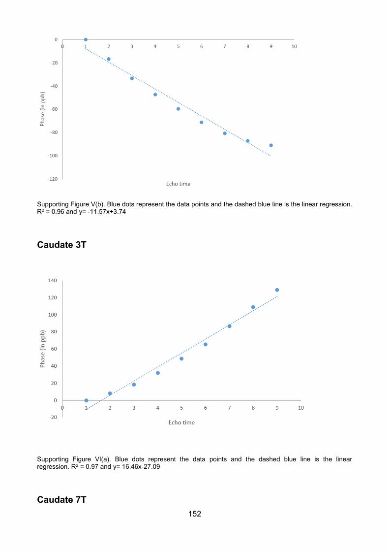
152
Caudate 3T
Caudate 7T
Supporting Figure V(b). Blue dots represent the data points and the dashed blue line is the linear regression. R2 = 0.96 and y= -11.57x+3.74
Supporting Figure VI(a). Blue dots represent the data points and the dashed blue line is the linear regression. R2 = 0.97 and y= 16.46x-27.09
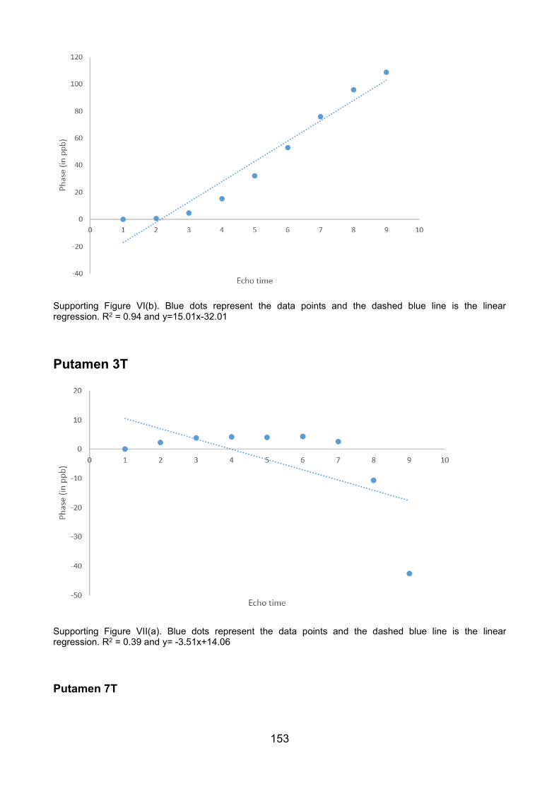
153
Putamen 3T
Putamen 7T
Supporting Figure VI(b). Blue dots represent the data points and the dashed blue line is the linear regression. R2 = 0.94 and y=15.01x-32.01
Supporting Figure VII(a). Blue dots represent the data points and the dashed blue line is the linear regression. R2 = 0.39 and y= -3.51x+14.06

154
Pallidum 3T
Pallidum 7T
Supporting Figure VII(b). Blue dots represent the data points and the dashed blue line is the linear regression. R2 = 0.98 and y= -8.69x+6.22
Supporting Figure VIII(a). Blue dots represent the data points and the dashed blue line is the linear regression. R2 = 0.95 and y= -37.16x+58.75

155
Thalamus 3T
Thalamus 7T
Supporting Figure VIII(b). Blue dots represent the data points and the dashed blue line is the linear regression. R2 = 0.99 and y= -25.89x+21.81
Supporting Figure IX(a). Blue dots represent the data points and the dashed blue line is the linear regression. R2 = 0.90 and y= -21.15x+43.33
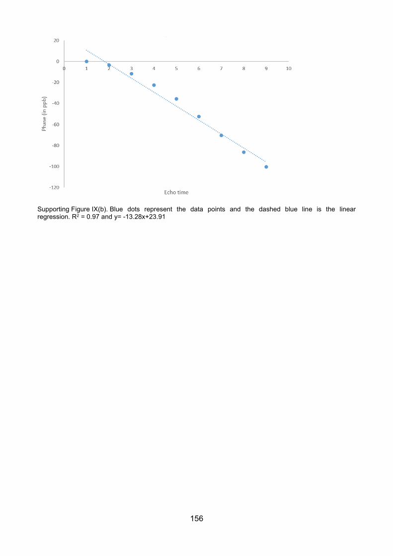
156
Supporting Figure IX(b). Blue dots represent the data points and the dashed blue line is the linear regression. R2 = 0.97 and y= -13.28x+23.91

157
Appendix 4.
As it is already explained in Section 5.3.2 to assist convergence to an optimal solution, we
up sampled our nine echo point complex signal to 17 echo time points (i.e. inserted one
echo time point between all measurements) using the interp1 function in MATLAB®. Nam
et al. (81) computed myelin water fraction maps using 16, 24 and 32 echo time points, and
found 16 echo time points were able to produce consistent fitting as measured by
parameter variations. To further support our findings, the 30 echo data from the study in
Chapter 3 was reduced to 15 echo monopolar data by removing every second echo.
Susceptibility maps were computed for the 15 echoes. 7 more middle echoes were
removed from the 15 echo data set reducing it to an 8 echo data set. An eight echo data
set was up sampled to a 15 echo data set with interp1 function in Matlab®. This up
sampled data is compared to the monopolar data computed earlier. With the assumption
from Nam et al., we found the data evolves smoothly as a function of echo time. We found
up sampled points are highly similar to the monopolar points. The up sampling is
performed in the caudate, internal capsule, red nucleus, corpus callosum, thalamus,
pallidum, substantia nigra, putamen, fornix, and insula as shown below in the figures:
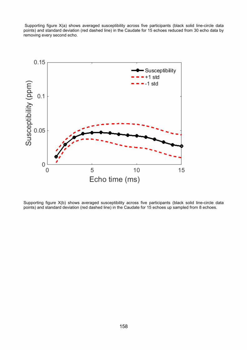
158
Supporting figure X(a) shows averaged susceptibility across five participants (black solid line-circle data points) and standard deviation (red dashed line) in the Caudate for 15 echoes reduced from 30 echo data by removing every second echo.
Supporting figure X(b) shows averaged susceptibility across five participants (black solid line-circle data points) and standard deviation (red dashed line) in the Caudate for 15 echoes up sampled from 8 echoes.
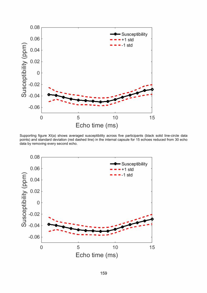
159
Supporting figure XI(a) shows averaged susceptibility across five participants (black solid line-circle data points) and standard deviation (red dashed line) in the internal capsule for 15 echoes reduced from 30 echo data by removing every second echo.

160
Supporting figure XI(b) shows averaged susceptibility across five participants (black solid line-circle data points) and standard deviation (red dashed line) in the internal capsule for 15 echoes up sampled from 8 echoes..
Supporting figure XII(a) shows averaged susceptibility across five participants (black solid line-circle data points) and standard deviation (red dashed line) in the red nucleus for 15 echoes reduced from 30 echo data by removing every second echo.
.
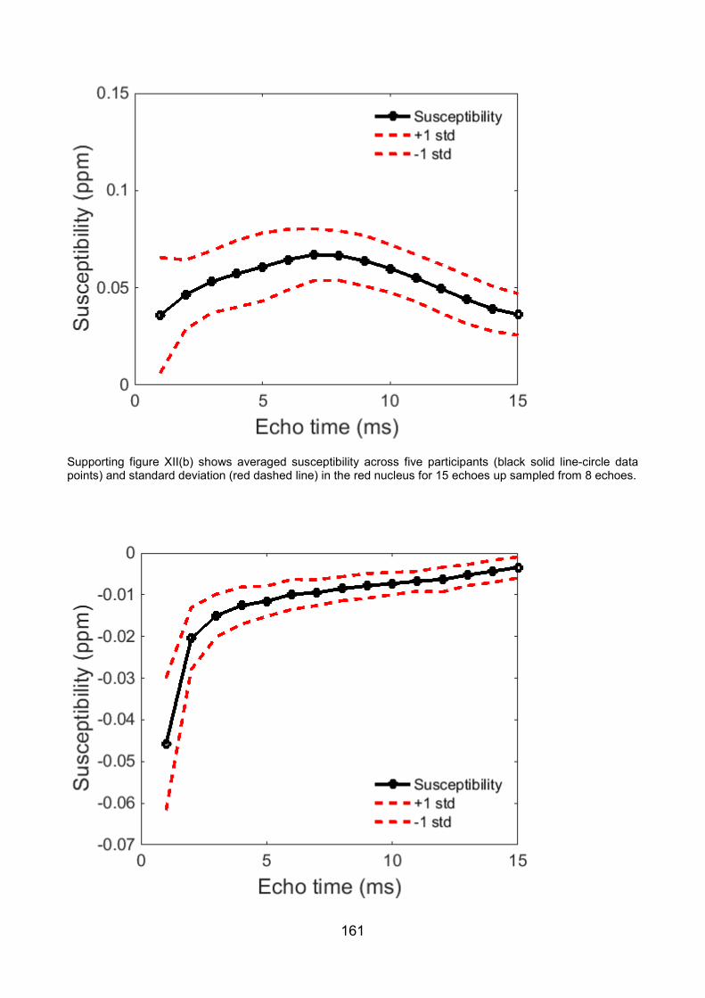
161
Supporting figure XII(b) shows averaged susceptibility across five participants (black solid line-circle data points) and standard deviation (red dashed line) in the red nucleus for 15 echoes up sampled from 8 echoes.

162
Supporting figure XIII(a) shows averaged susceptibility across five participants (black solid line-circle data points) and standard deviation (red dashed line) in the corpus callosum for 15 echoes reduced from 30 echo data by removing every second echo.
Supporting figure XIII(b) shows averaged susceptibility across five participants (black solid line-circle data points) and standard deviation (red dashed line) in the corpus callosum for 15 echoes up sampled from 8 echoes.

163
Supporting figure XIV(a) shows averaged susceptibility across five participants (black solid line-circle data points) and standard deviation (red dashed line) in the thalamus for 15 echoes reduced from 30 echo data by removing every second echo.
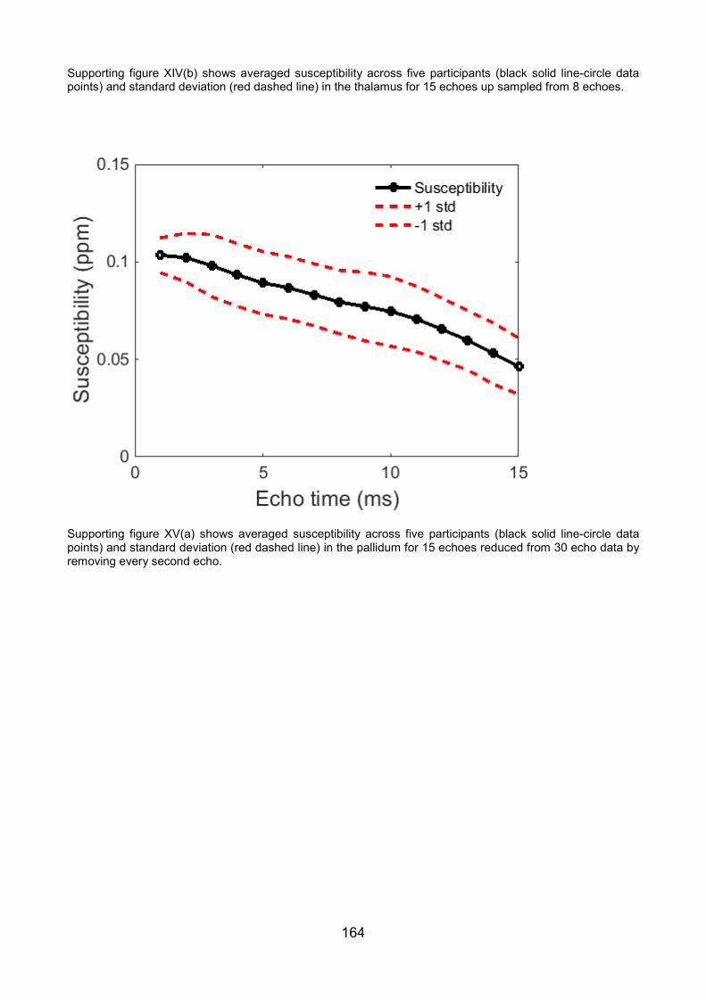
164
Supporting figure XIV(b) shows averaged susceptibility across five participants (black solid line-circle data points) and standard deviation (red dashed line) in the thalamus for 15 echoes up sampled from 8 echoes.
Supporting figure XV(a) shows averaged susceptibility across five participants (black solid line-circle data points) and standard deviation (red dashed line) in the pallidum for 15 echoes reduced from 30 echo data by removing every second echo.

165
Supporting figure XV(b) shows averaged susceptibility across five participants (black solid line-circle data points) and standard deviation (red dashed line) in the pallidum for 15 echoes up sampled from 8 echoes.
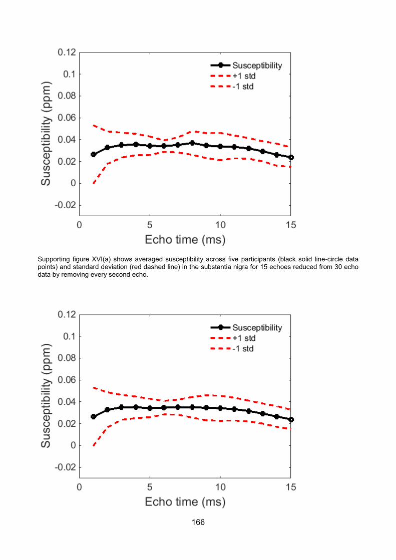
166
Supporting figure XVI(a) shows averaged susceptibility across five participants (black solid line-circle data points) and standard deviation (red dashed line) in the substantia nigra for 15 echoes reduced from 30 echo data by removing every second echo.

167
Supporting figure XVI(b) shows averaged susceptibility across five participants (black solid line-circle data points) and standard deviation (red dashed line) in the substantia nigra for 15 echoes up sampled from 8 echoes.
Supporting figure XVII(a) shows averaged susceptibility across five participants (black solid line-circle data points) and standard deviation (red dashed line) in the putamen for 15 echoes reduced from 30 echo data by removing every second echo.

168
Supporting figure XVII(b) shows averaged susceptibility across five participants (black solid line-circle data points) and standard deviation (red dashed line) in the putamen for 15 echoes up sampled from 8 echoes.

169
Supporting figure XVIII(a) shows averaged susceptibility across five participants (black solid line-circle data points) and standard deviation (red dashed line) in the fornix for 15 echoes reduced from 30 echo data by removing every second echo.
Supporting figure XVIII(b) shows averaged susceptibility across five participants (black solid line-circle data points) and standard deviation (red dashed line) in the fornix for 15 echoes up sampled from 8 echoes.

170
Supporting figure XIX(a) shows averaged susceptibility across five participants (black solid line-circle data points) and standard deviation (red dashed line) in the insula for 15 echoes reduced from 30 echo data by removing every second echo.

171
Supporting figure XIX(b) shows averaged susceptibility across five participants (black solid line-circle data points) and standard deviation (red dashed line) in the insula for 15 echoes up sampled from 8 echoes.