Measuring the Impacts of Teachers II: Teacher Value-Added ... · Measuring the Impacts of Teachers...

Measuring the Impacts of Teachers II: Teacher

Value-Added and Student Outcomes in Adulthood

By RAJ CHETTY, JOHN N. FRIEDMAN, AND JONAH E. ROCKOFF∗

Are teachers’ impacts on students’ test scores (“value-added”) a good

measure of their quality? This question has sparked debate partly be-

cause of a lack of evidence on whether high value-added (VA) teach-

ers improve students’ long-term outcomes. Using school district and

tax records for more than one million children, we find that students as-

signed to high-VA teachers are more likely to attend college, earn higher

salaries, and are less likely to have children as teenagers. Replacing a

teacher whose VA is in the bottom 5% with an average teacher would

increase the present value of students’ lifetime income by approximately

$250,000 per classroom.

How can we measure and improve the quality of teaching in primary schools? One

prominent but controversial method is to evaluate teachers based on their impacts on

students’ test scores, commonly termed the “value-added” (VA) approach.1 School

districts from Washington D.C. to Los Angeles have begun to calculate VA measures and

use them to evaluate teachers. Advocates argue that selecting teachers on the basis of

their VA can generate substantial gains in achievement (e.g., Gordon, Kane, and Staiger

2006, Hanushek 2009), while critics contend that VA measures are poor proxies for

teacher quality (e.g., Baker et al. 2010, Corcoran 2010). The debate about teacher VA

stems primarily from two questions. First, do the differences in test-score gains across

teachers measured by VA capture causal impacts of teachers or are they biased by student

sorting? Second, do teachers who raise test scores improve their students’ outcomes in

∗ Chetty: Harvard University, Littauer Center 226, Cambridge MA 02138 (e-mail: [email protected]); Fried-

man: Harvard University, Taubman Center 356, Cambridge MA 02138 (e-mail: [email protected]); Rockoff:

Columbia University, Uris 603, New York NY 10027 (e-mail: [email protected]).We are indebted to Gary

Chamberlain, Michal Kolesar, and Jesse Rothstein for many valuable discussions. We also thank Joseph Altonji, Josh

Angrist, David Card, David Deming, Caroline Hoxby, Guido Imbens, Brian Jacob, Thomas Kane, Lawrence Katz, Adam

Looney, Phil Oreopoulos, Douglas Staiger, Danny Yagan, anonymous referees, the editor, and numerous seminar par-

ticipants for helpful comments. This paper is the first of two companion papers on teacher quality. The results in

the two papers were previously combined in NBER Working Paper No. 17699, entitled “The Long-Term Impacts of

Teachers: Teacher Value-Added and Student Outcomes in Adulthood,” issued in December 2011. On May 4, 2012, Raj

Chetty was retained as an expert witness by Gibson, Dunn, and Crutcher LLP to testify about the importance of teacher

effectiveness for student learning in Vergara v. California based on the findings in NBER Working Paper No. 17699.

John Friedman is currently on leave from Harvard, working at the National Economic Council; this work does not rep-

resent the views of the NEC. All results based on tax data contained in this paper were originally reported in an IRS

Statistics of Income white paper (Chetty, Friedman, and Rockoff 2011a). Sarah Abraham, Alex Bell, Peter Ganong,

Sarah Griffis, Jessica Laird, Shelby Lin, Alex Olssen, Heather Sarsons, Michael Stepner, and Evan Storms provided out-

standing research assistance. Financial support from the Lab for Economic Applications and Policy at Harvard and the

National Science Foundation is gratefully acknowledged. Publicly available portions of the analysis code are posted at:

http://obs.rc.fas.harvard.edu/chetty/va_bias_code.zip1Value-added models of teacher quality were pioneered by Hanushek (1971) and Murnane (1975). More recent

examples include Rockoff (2004), Rivkin, Hanushek, and Kain (2005), Aaronson, Barrow, and Sander (2007), and Kane

and Staiger (2008).

1

2 THE AMERICAN ECONOMIC REVIEW

adulthood or are they simply better at teaching to the test?

We addressed the first question in the previous paper in this volume (Chetty, Fried-

man, and Rockoff 2014) and concluded that VA measures that control for lagged test

scores exhibit little or no bias. This paper addresses the second question.2 We study

the long-term impacts of teachers by linking information from an administrative dataset

on students and teachers in grades 3-8 from a large urban school district spanning 1989-

2009 with selected data from United States tax records spanning 1996-2011. We match

approximately 90% of the observations in the school district data to the tax data, allowing

us to track approximately one million individuals from elementary school to early adult-

hood, where we measure outcomes such as earnings, college attendance, and teenage

birth rates.

We use two research designs to estimate the long-term impacts of teacher quality:

cross-sectional comparisons across classrooms and a quasi-experimental design based

on teacher turnover. The first design compares the outcomes of students who were as-

signed to teachers with different VA, controlling for a rich set of student characteristics

such as prior test scores and demographics. We implement this approach by regress-

ing long-term outcomes on the test-score VA estimates constructed in Chetty, Friedman,

and Rockoff (2014). The identification assumption underlying this research design is

selection on observables: unobserved determinants of outcomes in adulthood such as

student ability must be unrelated to teacher VA conditional on the observable charac-

teristics. Although this is a very strong assumption, the estimates from this approach

closely match the quasi-experimental estimates for outcomes where we have adequate

precision to implement both designs, supporting its validity.

We find that teacher VA has substantial impacts on a broad range of outcomes. A 1 SD

improvement in teacher VA in a single grade raises the probability of college attendance

at age 20 by 0.82 percentage points, relative to a sample mean of 37%. Improvements in

teacher quality also raise the quality of the colleges that students attend, as measured by

the average earnings of previous graduates of that college. Students who are assigned

higher VA teachers have steeper earnings trajectories in their 20s. At age 28, the old-

est age at which we currently have a sufficiently large sample size to estimate earnings

impacts, a 1 SD increase in teacher quality in a single grade raises annual earnings by

1.3%. If the impact on earnings remains constant at 1.3% over the lifecycle, students

would gain approximately $39,000 on average in cumulative lifetime income from a 1

SD improvement in teacher VA in a single grade. Discounting at a 5% rate yields a

present value gain of $7,000 at age 12, the mean age at which the interventions we study

occur. We also find that improvements in teacher quality significantly reduce the proba-

bility of having a child while being a teenager, increase the quality of the neighborhood

in which the student lives (as measured by the percentage of college graduates in that

ZIP code) in adulthood, and raise participation rates in 401(k) retirement savings plans.

Our second design relaxes the assumption of selection on observables by exploiting

2Recent work has shown that early childhood education has significant long-term impacts (e.g. Heckman et al. 2010a,

2010b, Chetty et al. 2011), but there is no evidence to date on the long-term impacts of teacher quality as measured by

value-added.

LONG-TERM IMPACTS OF TEACHERS 3

teacher turnover as a quasi-experimental source of variation in teacher quality. To un-

derstand this research design, suppose a high-VA 4th grade teacher moves from school

A to another school in 1995. Because of this staff change, students entering grade 4

in school A in 1995 will have lower quality teachers on average than those in the prior

cohort. If high VA teachers improve long-term outcomes, we would expect college at-

tendance rates and earnings for the 1995 cohort to be lower on average than the previous

cohort. Building on this idea, we estimate teachers’ impacts by regressing changes in

mean adult outcomes across consecutive cohorts of children within a school on changes

in the mean VA of the teaching staff.

Using this design, we find that a 1 SD improvement in teacher VA raises the probability

of college attendance at age 20 by 0.86 percentage points, nearly identical to the estimate

obtained from our first research design. Improvements in average teacher VA also in-

crease the quality of colleges that students attend. The impacts on college outcomes are

statistically significant with p < 0.01. Unfortunately, we have insufficient precision to

obtain informative estimates for earnings using the quasi-experimental design.

Our quasi-experimental results rest on the identification assumption that high-frequency

teacher turnover within school-grade cells is uncorrelated with student and school char-

acteristics. Several pieces of evidence support this assumption. First, predetermined stu-

dent and parent characteristics are uncorrelated with changes in the quality of teaching

staff. Second, students’ prior test scores and contemporaneous scores in the other sub-

ject are also uncorrelated with changes in the quality of teaching staff in a given subject.

Third, changes in teacher VA across cohorts have sharp effects on college attendance

exactly in the year of the change but not in prior years or subsequent years.

The long-term impacts of teacher VA are slightly larger for females than males. Im-

provements in English teacher quality have larger impacts than improvements in math

teacher quality. The impacts of teacher VA are roughly constant in percentage terms by

parents’ income. Hence, higher income households, whose children have higher earn-

ings on average, should be willing to pay larger amounts for higher teacher VA. Teach-

ers’ impacts are significant and large throughout grades 4-8, showing that improvements

in the quality of education can have large returns well beyond early childhood.

Our conclusion that teachers have long-lasting impacts may be surprising given evi-

dence that teachers’ impacts on test scores “fade out” very rapidly in subsequent grades

(Rothstein 2010, Carrell and West 2010, Jacob, Lefgren, and Sims 2010). We confirm

this rapid fade-out in our data, but find that teachers’ impacts on earnings are similar to

what one would predict based on the cross-sectional correlation between earnings and

contemporaneous test score gains. This pattern of fade-out and re-emergence echoes the

findings of recent studies of early childhood interventions (Deming 2009, Heckman et

al. 2010b, Chetty et al. 2011).

To illustrate the magnitude of teachers’ impacts, we evaluate Hanushek’s (2009) pro-

posal to replace teachers in the bottom 5% of the VA distribution with teachers of average

quality. We estimate that replacing a teacher whose current VA is in the bottom 5 per-

cent with an average teacher would increase the mean present value of students’ lifetime

income by $250,000 per classroom over a teacher’s career, accounting for drift in teacher


quality over time.3 However, because VA is estimated with noise, the gains from des-

electing teachers based on data from a limited number of classrooms are smaller. The

present value gain from deselecting the bottom 5% of teachers using three years of test

score data is $185,000 per classroom on average.4 This gain is still about 10 times larger

than recent estimates of the additional salary one would have to pay teachers to compen-

sate them for the risk of evaluation based on VA measures (Rothstein 2013). This result

suggests that VA could potentially be a useful tool for evaluating teacher performance if

the signal quality of VA for long-term impacts does not fall substantially when it is used

to evaluate teachers.

We also evaluate the expected gains from policies that pay bonuses to high-VA teachers

to increase retention rates. The gains from such policies are only slightly larger than their

costs because most bonus payments end up going to high-VA teachers who would have

stayed even without the additional payment. Replacing low VA teachers may therefore

be a more cost effective strategy to increase teacher quality in the short run than paying

bonuses to retain high-VA teachers. In the long run, higher salaries could attract more

high VA teachers to the teaching profession, a potentially important benefit that we do

not measure here.

The paper is organized as follows. In Section I, we formalize our estimating equa-

tions and explain how the parameters we estimate should be interpreted using a simple

statistical model. Section II describes the data sources and reports summary statistics as

well as cross-sectional correlations between test scores and adult outcomes. Sections III

and IV present results on teachers’ long-term impacts using the two research designs de-

scribed above. We analyze the heterogeneity of teachers’ impacts in Section V. Section

VI presents policy simulations and Section VII concludes.

I. Conceptual Framework

In this section, we first present a simple statistical model of students’ long-term out-

comes as a function of their teachers’ value-added. We then describe how the reduced-

form parameters of this statistical model should be interpreted. Finally, we show how we

estimate the impacts of teacher VA on long-term outcomes given that each teacher’s true

value-added is unobserved.

Statistical Model. Consider the outcomes of a student i who is in grade g in calendar

year ti (g). Let j = j (i, t) denote student i’s teacher in school year t ; for simplicity,

assume that the student has only one teacher throughout the school year, as in elementary

schools. Let µ j t represent teacher j’s “test-score value-added” in year t , so that student

i’s test score in year t is

(1) A∗i t = βXi t + µ j t + εi t .

3This calculation discounts the earnings gains at a rate of 5% to age 12. The estimated total undiscounted earnings

gains from this policy are approximately $50,000 per child and $1.4 million for the average classroom.4The gains remain substantial despite noise because very few of the teachers with low VA estimates ultimately turn

out to be excellent teachers. For example, we estimate that 3.2% of the math teachers in elementary school whose

estimated VA is in the bottom 5% based on three years of data actually have true VA above the median.


Here, Xi t denotes observable determinants of student achievement, such as lagged test

scores and family characteristics and εi t denotes a student-level error that may be corre-

lated across students within a classroom and with teacher value-added µ j t . We scale µ j t

in student test-score SDs so that the average teacher has µ j t = 0 and the effect of a 1 unit

increase in teacher value-added on end-of-year test scores is 1. We allow teacher quality

µ j t to vary with time t to account for the stochastic drift in teacher quality documented

in our companion paper (Chetty, Friedman, and Rockoff 2014).

Let Y ∗i denote student i’s earnings in adulthood. Throughout our analysis, we focus

on earnings residuals after removing the effect of observable characteristics:

(2) Yi t = Y ∗i − βY Xi t

The earnings residuals Yi t vary across school years because the control vector Xi t varies

across school years. We estimate the coefficient vector βY using variation across stu-

dents taught by the same teacher using an OLS regression

(3) Y ∗i = α j + βY Xi t

where α j is a teacher fixed effect. Importantly, we estimate βY using within-teacher

variation to account for the potential sorting of students to teachers based on VA. If

teacher VA is correlated with Xi t , estimates of βY in a specification without teacher

fixed effects are biased because part of the teacher effect is attributed to the covariates.

See Section I.B of our companion paper for further discussion of this issue.

We model the relationship between earnings residuals and teacher VA in school year t

using the following linear specification:

(4) Yi t = a + κgm j t + ηi t

where m j t = µ j t/σµ denotes teacher j’s “normalized value-added” (i.e., teacher quality

scaled in standard deviation (σµ) units of the teacher VA distribution).

Interpretation of Reduced-Form Treatment Effects. The parameter κg in (4) represents

the reduced-form impact of a 1 SD increase in teachers’ test-score VA in a given school

year t on earnings. There are two important issues to keep in mind when interpreting

this parameter, which we formalize using a dynamic model of education production in

Appendix A.

First, the reduced-form impact combines two effects: the direct impact of having a

higher VA teacher in grade g and the indirect impact of endogenous changes in other

educational inputs. For example, other determinants of earnings such as investments in

learning by children and their parents might respond endogenously to changes in teacher

quality. One particularly important endogenous response is that a higher achieving stu-

dent may be tracked into classes taught by higher quality teachers. Such tracking would

lead us to overstate the impacts of improving teacher quality in grade g holding fixed

the quality of teachers in subsequent grades. In Section V.C, we estimate the degree

of teacher tracking and use these estimates to identify the impact of having a higher VA


teacher in each grade holding fixed future teacher quality, which we denote by κg. The

degree of tracking turns out to be relatively small in our data, and thus the reduced-

form estimates of κg reported below are similar to the net impacts of each teacher κg.5

Although the net impacts κg still combine several structural parameters – such as endoge-

nous responses by parents and children to changes in teacher quality – they are relevant

for policy. For example, the ultimate earnings impact of retaining teachers on the basis

of their VA depends on κg.

Second, κg measures only the portion of teachers’ earnings impacts that are correlated

with their impacts on test scores. As a result, κg is a lower bound for the standard de-

viation of teachers’ effects on earnings. Intuitively, some teachers may be effective at

raising students’ earnings even if they are not effective at raising test scores, for instance

by directly instilling other skills that have long-term payoffs (Jackson 2013). In prin-

ciple, one could estimate teacher j’s “earnings value-added” (µYjt ) based on the mean

residual earnings of her students, exactly as we estimated test-score VA in our first pa-

per. Unfortunately, the orthogonality condition required to obtain unbiased forecasts of

teachers’ earnings VA – that students’ earnings are orthogonal to earnings VA estimates

– does not hold in practice, as we discuss in Appendix A. We therefore focus on es-

timating the effect of being assigned to a high test-score VA teacher on earnings (κg).

Although κg does not correspond directly to earnings VA, it reveals the extent to which

the test-score based VA measures currently used by school districts are informative about

teachers’ long-term impacts.

Empirical Implementation. There are two challenges in estimating κg using (4). First,

unobserved determinants of earnings ηi t may be correlated with teacher VA m j t . We

return to this issue in our empirical analysis and isolate variation in teacher VA that is

orthogonal to unobserved determinants of earnings. Second, teachers’ true test-score

VA m j t is unobserved. We can solve this second problem by substituting estimates of

teacher VA m j t = µ j t/σµ for true teacher VA in (4) under the following assumption.

Assumption 1 [Forecast Unbiasedness of Test-Score VA] Test-score value-added esti-

mates µ j t are forecast unbiased:

Cov(µ j t , µ j t

)V ar

(µ j t

) =Cov

(m j t , m j t

)V ar

(m j t

) = 1.

In our companion paper, we demonstrate that Assumption 1 holds for the VA estimates

that we use in this paper. Equation (4) implies that Cov(Yi t , m j t

)= κgCov

(m j t , m j t

)+

Cov(ηi t , m j t). Hence, under Assumption 1,

Cov(Yi t , m j t

)V ar

(m j t

) = κg +Cov

(ηi t , m j t

)V ar

(m j t

) .

5An alternative approach to identify the direct impacts of teachers in each grade g would be to include teacher VA

in all grades simultaneously in the model in (4). Unfortunately, this is not feasible because our primary research design

requires conditioning on lagged test scores and lagged scores are endogenous to teacher quality in the previous grade.

For the same reason, we also cannot identify the substitutability or complementarity of teachers’ impacts across grades.

See Appendix A for further details.


It follows that we can identify the impact of a 1 SD increase in a teacher’s true VA m j t

from an OLS regression of earnings residuals Yi t on teacher VA estimates m j t ,

(5) Yi t = α + κgm j t + η′i t ,

provided that unobserved determinants of earnings are orthogonal to teacher VA esti-

mates m j t .

Intuitively, we identify κg using 2SLS by instrumenting for true teacher VA m j t with

the teacher VA estimates we constructed in our companion paper. Forecast unbiasedness

of test-score VA implies that the first stage of this 2SLS regression has a coefficient of 1.

Thus, the reduced form coefficient obtained from an OLS regression of earnings on VA

estimates identifies κg.

The remainder of the paper focuses on estimating variants of (5).6

II. Data

We draw information from two databases: administrative school district records and

federal income tax records. This section describes the two data sources and the struc-

ture of the linked analysis dataset. We then provide descriptive statistics and report

correlations between test scores and long-term outcomes as a benchmark to interpret the

magnitude of the causal effects of teachers. Note that the dataset we use in this paper is

identical to that used in our first paper, except that we restrict attention to the subset of

students who are old enough for us to observe outcomes in adulthood by 2011.

A. School District Data

We obtain information on students, including enrollment history, test scores, and teacher

assignments from the administrative records of a large urban school district. These data

span the 1988-1989 through 2008-2009 school years and cover roughly 2.5 million chil-

dren in grades 3-8. For simplicity, we refer to school years by the year in which the

spring term occurs (e.g., the school year 1988-1989 is 1989). We summarize the key

features of the data relevant for our analysis of teachers’ long-term impacts here; see

Section II of our first paper for a comprehensive description of the school district data.

Test Scores. The data include approximately 18 million test scores. Test scores are

available for English language arts and math for students in grades 3-8 in every year

from the spring of 1989 to 2009, with the exception of 7th grade English scores in 2002.

We follow prior work by normalizing the official scale scores from each exam to have

mean zero and standard deviation one by year and grade. The within-grade variation

in achievement in the district we examine is comparable to the within-grade variation

nationwide, so our results can be compared to estimates from other samples.

Demographics. The dataset contains information on ethnicity, gender, age, receipt

of special education services, and limited English proficiency for the school years 1989

6Another way to identify κg is to directly estimate the covariance of teachers’ effects on earnings (µYjt

) and test

scores (µ j t ) in a correlated random effects or factor model. Chamberlain (2013) develops such an approach and obtains

estimates similar to those reported here.


through 2009. The database used to code special education services and limited English

proficiency changed in 1999, creating a break in these series that we account for in our

analysis by interacting these two measures with a post-1999 indicator. Information on

free and reduced price lunch is available starting in school year 1999.

Teachers. The dataset links students in grades 3-8 to classrooms and teachers from

1991 through 2009. This information is derived from a data management system which

was phased in over the early 1990s, so not all schools are included in the first few years

of our sample. In addition, data on course teachers for middle and junior high school

students – who, unlike students in elementary schools, are assigned different teachers

for math and English – are more limited. Course teacher data are unavailable prior to

the school year 1994, then grow in coverage to roughly 60% by school year 1998 and

85% by 2003. These missing teacher links raise two potential concerns. First, our

estimates (especially for grades 6-8) apply to a subset of schools with more complete

information reporting systems and thus may not be representative of the district as a

whole. Reassuringly, we find that these schools do not differ significantly from the

sample as a whole on test scores and other observables. Second, and more importantly,

missing data could generate biased estimates. We address this concern by showing that

our estimates remain similar in a subsample of school-grade-subject cells with little or

no missing data (Appendix Table 7).

Sample Restrictions. Starting from the raw dataset, we make a series of restrictions that

parallel those in prior work to obtain our primary school district sample. First, because

our estimates of teacher value-added always condition on prior test scores, we restrict

our sample to grades 4-8, where prior test scores are available. Second, we exclude the

6% of observations in classrooms where more than 25 percent of students are receiving

special education services, as these classrooms may be taught by multiple teachers or

have other special teaching arrangements. We also drop the 2% of observations where

the student is listed as receiving instruction at home, in a hospital, or in a school serving

solely disabled students. Third, we drop classrooms with less than 10 students or more

than 50 students as well as teachers linked with more than 200 students in a single grade,

because such students are likely to be mis-linked to classrooms or teachers (0.5% of

observations). Fourth, when a teacher is linked to students in multiple schools during

the same year, which occurs for 0.3% of observations, we use only the links for the school

where the teacher is listed as working according to human resources records and set the

teacher as missing in the other schools. Finally, because the adult outcomes we analyze

are measured at age 20 or afterward, in this paper we restrict the sample to students who

would have graduated high school by the 2008-09 school year (and thus turned 20 by

2011) if they progressed through school at a normal pace.7

7A few classrooms contain students at different grade levels because of retentions or split-level classroom structures.

To avoid dropping a subset of students within a classroom, we include every classroom that has at least one student who

would graduate school during or before 2008-09 if she progressed at the normal pace. That is, we include all classrooms

in which mini (12+ school year − gradei ) ≤ 2009.


B. Tax Data

We obtain information on students’ outcomes in adulthood from U.S. federal income

tax returns spanning 1996-2011.8 The school district records were linked to the tax data

using an algorithm based on standard identifiers (date of birth, state of birth, gender,

and names) described in Appendix C of our companion paper, after which individual

identifiers were removed to protect confidentiality. 87.4% of the students and 89.2% of

student-subject-year observations in the sample used to analyze long-term impacts were

matched to the tax data.9 We define students’ outcomes in adulthood as follows.

Earnings. Individual wage earnings data come from W-2 forms, which are available

from 1999-2011. Importantly, W-2 data are available for both tax filers and non-filers,

eliminating concerns about missing data on formal sector earnings. We cap earnings

in each year at $100,000 to reduce the influence of outliers; 1.3% of individuals in the

sample report earnings above $100,000 at age 28. We measure all monetary variables in

2010 dollars, adjusting for inflation using the Consumer Price Index. Individuals with

no W-2 are coded as having 0 earnings. 33.1% of individuals have 0 wage earnings at

age 28 in our sample.

Total Income. To obtain a more comprehensive definition of income, we define “total

income” as the sum of W-2 wage earnings and household self-employment earnings (as

reported on the 1040). For non-filers, we define total income as just W-2 wage earnings;

those with no W-2 income are coded as having zero total income. 29.6% of individuals

have 0 total income in our sample.10 We show that similar results are obtained using

this alternative definition of income, but use W-2 wage earnings as our baseline measure

because it (1) is unaffected by the endogeneity of tax filing and (2) provides a consistent

definition of individual (rather than household) income for both filers and non-filers.

College Attendance. We define college attendance as an indicator for having one or

more 1098-T forms filed on one’s behalf. Title IV institutions – all colleges and universi-

ties as well as vocational schools and other postsecondary institutions eligible for federal

student aid – are required to file 1098-T forms that report tuition payments or scholar-

ships received for every student. Because the 1098-T forms are filed directly by colleges

independent of whether an individual files a tax return, we have complete records on

college attendance for all individuals. The 1098-T data are available from 1999-2011.

Comparisons to other data sources indicate that 1098-T forms capture college enrollment

accurately (see Appendix B).

College Quality. We construct an earnings-based index of college quality based on

data from the universe of tax returns (not just the students from our school district). Us-

ing the population of all current U.S. citizens born in 1979 or 1980, we group individuals

8Here and in what follows, the year refers to the tax year, i.e. the calendar year in which income is earned. In most

cases, tax returns for tax year t are filed during the calendar year t + 1.9We find little or no correlation between match rates and teacher VA in the various subsamples we use in our analysis

and obtain very similar estimates of teachers’ impacts on long-term outcomes when restricting the sample to school-

grade-subject cells with above-median match rates (see Appendix Table 7).10According to the Current Population Survey, 27.2% of the non-institutionalized population between the ages of 25

and 29 was not employed in 2011. The non-employment rate in our sample may differ from this figure because it includes

the institutionalized population in the denominator and applies to a relatively low-income urban public school district.


by the higher education institution they attended at age 20. We pool individuals who

were not enrolled in any college at age 20 together in a separate “no college” category.

For each college or university (including the “no college” group), we then compute the

mean W-2 earnings of the students when they are age 31 (in 2010 and 2011). Among

colleges attended by students in the school district studied in this paper, the average

value of our earnings index is $44,048 for four-year colleges and $30,946 for two-year

colleges. For students who did not attend college, the mean earnings level is $17,920.

In Appendix B, we analyze the robustness of the college quality index to alternative

specifications, such as measuring earnings and college attendance at different ages and

defining the index based on total income instead of W-2 earnings. We find that rankings

of college quality are very stable across cohorts and are robust to alternative specifica-

tions provided that earnings are measured after age 28 (Appendix Figure 1, Appendix

Table 2).

Neighborhood Quality. We use data from 1040 forms to identify each household’s

ZIP code of residence in each year. For non-filers, we use the ZIP code of the address

to which the W-2 form was mailed. If an individual did not file and has no W-2 in a

given year, we impute current ZIP code as the last observed ZIP code. We construct a

measure of a neighborhood’s SES using data on the percentage of college graduates in

the individual’s ZIP code from the 2000 Census.

Retirement Savings. We measure retirement savings using contributions to 401(k)

accounts reported on W-2 forms from 1999-2011. We define saving for retirement as an

indicator for contributing to a 401(k) at age 28.

Teenage Birth. We define a woman as having a teenage birth if she ever claims a

dependent who was born while she was between the ages of 13 and 19 (as of 12/31 in

the year the child was born). This measure is an imperfect proxy for having a teenage

birth because it only covers children who are claimed as dependents by their mothers

and includes any other dependents who are not biological children but were born while

the mother was a teenager. Despite these limitations, our proxy for teenage birth is

closely aligned with estimates based on the American Community Survey (ACS). 15.8%

of women in our core sample have teenage births, compared with 14.6% in the 2003

ACS. The unweighted correlation between state-level teenage birth rates in our data and

the ACS is 0.80.

Parent Characteristics. We also use the tax data to obtain information on five parent

characteristics that we use as controls. Students were linked to parents based on the

earliest 1040 form filed between tax years 1996 and 2011 on which the student was

claimed as a dependent. We identify parents for 94.8% of the observations in the analysis

dataset conditional on being matched to the tax data.11

We define parental household income as mean Adjusted Gross Income (capped at

$117,000, the 95th percentile in our sample) between 2005 and 2007 for the primary

11The remaining students are likely to have parents who did not file tax returns in the early years of the sample when

they could have claimed their child as a dependent, making it impossible to link the children to their parents. Note that

this definition of parents is based on who claims the child as a dependent, and thus may not reflect the biological parent

of the child.


filer who first claimed the child.12 Parents are assigned an income of 0 in years when

they did not file a tax return. We define parental marital status, home ownership, and

401(k) saving as indicators for whether the first primary filer who claims the child ever

files a joint tax return, makes a mortgage interest payment (based on data from 1040’s

for filers and 1099’s for non-filers), or makes a 401(k) contribution (based on data from

W-2’s) between 2005 and 2007. Lastly, we define mother’s age at child’s birth using data

from Social Security Administration records on birth dates for parents and children. For

single parents, we define the mother’s age at child’s birth using the age of the filer who

first claimed the child, who is typically the mother but is sometimes the father or another

relative.13 When a child cannot be matched to a parent, we define all parental charac-

teristics as zero, and we always include a dummy for missing parents in regressions that

include parent characteristics.

C. Summary Statistics

The linked school district and tax record analysis dataset has one row per student per

subject (math or English) per school year, as illustrated in Appendix Table 1. Each

observation in the analysis dataset contains the student’s test score in the relevant sub-

ject test, demographic information, and class and teacher assignment if available. Each

row also includes all the students’ available adult outcomes (e.g. college attendance and

earnings at each age). We organize the data in this format so that each row contains

information on a treatment by a single teacher conditional on pre-determined character-

istics, facilitating the estimation of (5). We account for the fact that each student appears

multiple times in the dataset by clustering standard errors as described in Section III.A.

After imposing the sample restrictions described above, the linked analysis sample

contains 6.8 million student-subject-year observations (covering 1.1 million students)

that we use to study teachers’ long-term impacts.14 Table 1 reports summary statistics

for this sample. Note that the summary statistics are student-subject-year means and

thus weight students who are in the district for a longer period of time more heavily,

as does our empirical analysis. On average, each student has 6.25 subject-school year

observations.

The mean test score in the analysis sample is positive and has a standard deviation

below 1 because we normalize the test scores in the full population that includes students

in special education classrooms and schools (who typically have lower test scores). The

mean age at which students are observed in school is 11.7 years. 77.1% of students are

eligible for free or reduced price lunches.

12Because the children in our sample vary in age by over 25 years whereas the tax data start only in 1996, we cannot

measure parent characteristics at the same age for all children. For simplicity, we instead measure parent characteristics

at a fixed time. Measuring parent income at other points in time yields very similar results (not reported).13We set the mother’s age at child’s birth to missing for 78,007 observations in which the implied mother’s age at birth

based on the claiming parent’s date of birth is below 13 or above 65, or where the date of birth is missing entirely from

SSA records.14For much of the analysis in our first paper, we restricted attention to the subset of observations in the core sample

that have lagged scores and other controls needed to estimate the baseline VA model. Because we do not control for

individual-level variables in most of the specifications in this paper, we do not impose that restriction here.


The availability of data on adult outcomes naturally varies across cohorts. There are

more than 5.9 million observations for which we observe college attendance at age 20.

We observe earnings at age 25 for 2.3 million observations and at age 28 for 1.3 million

observations. Because many of these observations at later ages are from older cohorts

of students who were in middle school in the early 1990s, we were not able to obtain

information on teachers. As a result, there are only 1.6 million student-subject-school

year observations for which we see both teacher VA and earnings at age 25, 750,000 at

age 28, and only 220,000 at age 30. The oldest age at which the sample is large enough

to obtain informative estimates of teachers’ impacts on earnings turns out to be age 28.

Mean individual earnings at age 28 is $20,885, while mean total income is $21,272 (in

2010 dollars).

For students whom we are able to link to parents, the mean parent household income

is $40,808, while the median is $31,834. Though our sample includes more low income

households than would a nationally representative sample, it still includes a substantial

number of higher income households, allowing us to analyze the impacts of teachers

across a broad range of the income distribution. The standard deviation of parent income

is $34,515, with 10% of parents earning more than $100,000.

D. Cross-Sectional Correlations

Appendix Tables 3-6 report coefficients from OLS regressions of various adult out-

comes on test scores. Both math and English test scores are highly positively correlated

with earnings, college attendance, and neighborhood quality and are negatively corre-

lated with teenage births. In the cross-section, a 1 SD increase in test score is associated

with a $7,700 (36%) increase in earnings at age 28. Conditional on the student- and

class-level controls Xi t that we define in Section III.A below, a 1 SD increase in the

current test score is associated with $2,600 (12%) increase in earnings on average.

Appendix Figure 2 presents binned scatter plots of selected outcomes vs. test scores

both with and without controls. The unconditional relationship between scores and

outcomes is S-shaped, while the relationship conditional on prior scores and other co-

variates is almost perfectly linear. We return to these results below and show that the

causal impacts of teacher VA on earnings and other outcomes are commensurate to what

one would predict based on these correlations.

III. Research Design 1: Cross-Class Comparisons

Our first method of estimating teachers’ long-term impacts builds on our finding that

conditioning on prior test scores and other observables is adequate to obtain unbiased es-

timates of teachers’ causal impacts on test scores (Chetty, Friedman, and Rockoff 2014).

Given this result, one may expect that comparing the long-term outcomes of students

assigned to different teachers conditional on the same control vector will yield unbiased

estimates of teachers’ long-term impacts. The next subsection formalizes the identifica-

tion assumption and methodological details of this approach. We then present results for

three sets of impacts: college attendance, earnings, and other outcomes such as teenage

birth.


A. Methodology

We begin by constructing earnings (or other long-term outcome) residuals Yi t = Y ∗i −

βYXi t , estimating β

Yusing within-teacher variation as in (3). We then regress students’

earnings residuals on their teachers’ normalized VA m j t , pooling all grades and subjects:

(6) Yi t = α + κm j t + η′i t

Note that we do not residualize m j t with respect to the controls Xi t when estimating (6).

In a partial regression, one typically residualizes m j t with respect to Xi t because the OLS

regression of Y ∗i on Xi t used to construct earnings residuals yields an estimate of βY that

is biased by the correlation between and m j t and Xi t . This problem does not arise here

because we estimate βY from a regression with teacher fixed effects, so the variation in

Xi t used to identify βY is orthogonal to the variation in VA across teachers.15 Hence,

regressing Yi t directly on m j t identifies the relationship between Yi t and m j t conditional

on Xi t .

Recall that each student appears in our dataset once for every subject-year with the

same level of Yi t but different values of m j t . Hence, κ represents the mean impact of

having a higher VA teacher for a single grade between grades 4-8. We present results on

heterogeneity in impacts across grades and subgroups in Section V.

Estimating (6) using OLS yields an unbiased estimate of κ under the following as-

sumption.

Assumption 2 [Selection on Observables] Test-score value-added estimates are orthog-

onal to unobserved determinants of earnings conditional on Xi t :

(7) Cov(m j t , η

′i t

)= 0.

While we cannot be certain that conditioning on observables fully accounts for differ-

ences in student characteristics across teachers, as required by Assumption 2, the quasi-

experimental evidence reported in the next section supports this assumption. In partic-

ular, quasi-experimental estimates of the impacts of teacher quality on test scores and

college attendance are very similar to the estimates obtained from (6).16 This result sup-

ports the validity of the selection on observables assumption not only for test scores and

college attendance but also for other outcomes as well, as any selection effects would

presumably be manifested in all of these outcomes.

Four methodological issues arise in estimating (6): (1) estimating test-score VA m j t ,

15Teacher fixed effects account for correlation between Xi t and mean teacher VA. If Xi t is correlated with fluctuations

in teacher VA across years due to drift, one may still obtain biased estimates of βY . This problem is modest because only

20% of the variance in m j t is within teacher. Moreover, we obtain similar results when estimating m j t and βY from

regressions without teacher fixed effects and implementing a standard partial regression (Chetty, Friedman, and Rockoff

2011b). We estimate βY using within-teacher variation here for consistency with our approach to estimating teacher VA

in the first paper; see Section 2.2 of that paper for further details.16The test score results are reported in our companion paper. We do not have adequate precision to implement the

quasi-experimental design for earnings or within specific subgroups, which is why the cross-sectional estimates remain

valuable.


(2) specifying a control vector Xi t , (3) calculating the standard error on κ , and (4) ac-

counting for outliers in m j t . The remainder of this subsection addresses these four

issues. Note that our methodology closely parallels that in our companion paper. In

particular, we use the same VA estimates and control vectors and calculate standard er-

rors in the same way. We did not address outliers in our first paper because they only

affect our analysis of long-term impacts, as we explain below.

Estimating Test-Score VA. We define normalized VA m j t = µ j t/σµ, where µ j t is the

baseline estimate of test-score VA for teacher j in year t constructed in our companion

paper.17 We define σµ as the standard deviation of teacher effects for the corresponding

subject and school-level using the estimates in Table 2 of our companion paper: 0.163

for math and 0.124 for English in elementary school and 0.134 for math and 0.098 for

English in middle school. With this scaling, a 1 unit increase in m j t corresponds to a

teacher who is rated 1 SD higher in the distribution of true teacher quality for her subject

and school-level. Note that because µ j t is shrunk toward the sample mean to account for

noise in VA estimates, SD(µ j t) < σµ and hence the standard deviation of the normalized

VA measure m j t is less than 1. We demean m j t within each of the four subject (math vs.

English) by school level (elementary vs. middle) cells in the estimation sample in (6) so

that κ is identified purely from variation within the subject-by-school-level cells.

Importantly, the VA estimates m j t are predictions of teacher quality in year t based on

test score data from all years excluding year t . For example, when predicting teachers’

effects on the outcomes of students they taught in 1995, we estimate m j,1995 based on

residual test scores from students in all years of the sample except 1995. To maximize

precision, the VA estimates are based on data from all years for which school district data

with teacher assignments are available (1991-2009), not just the subset of older cohorts

for which we observe long-term outcomes.

Using a leave-year-out estimate of VA is necessary to obtain unbiased estimates of

teachers’ long-term impacts because of correlated errors in students’ test scores and later

outcomes. Intuitively, if a teacher is randomly assigned unobservably high ability stu-

dents, her estimated VA will be higher. The same unobservably high ability students are

likely to have high levels of earnings η′

i t , generating a mechanical correlation between

VA and earnings even if teachers have no causal effect (κ = 0). The leave-year-out

approach eliminates this correlated estimation error bias because m j t is estimated using

a sample that excludes the observations on the left hand side of (6).18

Control Vectors. We construct residuals Yi t using separate models for each of the four

subject-by-school-level cells. Within each of these groups, we regress raw outcomes

Y ∗i on a vector of covariates Xi t with teacher fixed effects, as in (3), and compute resid-

uals Yi t . We partition the control vector Xi t that we used to construct our baseline

VA estimates into two components: student-level controls XIi t that vary across students

within a class and classroom-level controls Xct that vary only at the classroom level.

17Unless otherwise specified, the independent variable in all the regressions and figures in this paper is normalized

test-score VA m j t . For simplicity, we refer to this measure as “value-added” or VA below.18This problem does not arise when estimating the impacts of treatments such as class size because the treatment is

observed; here, the size of the treatment (teacher VA) must itself be estimated, leading to correlated estimation errors.


The student-level control vector XIi t includes cubic polynomials in prior-year math and

English scores, interacted with the student’s grade level to permit flexibility in the per-

sistence of test scores as students age. We also control for the following student level

characteristics: ethnicity, gender, age, lagged suspensions and absences, and indicators

for grade repetition, free or reduced-price lunch, special education, and limited Eng-

lish. The class-level controls Xct consist of the following elements: (1) class size and

class-type indicators (honors, remedial), (2) cubics in class and school-grade means of

prior-year test scores in math and English (defined based on those with non-missing prior

scores) each interacted with grade, (3) class and school-year means of all the individual

covariates XIi t , and (4) grade and year dummies.

In our baseline analysis, we control only for the class-level controls Xct when estimat-

ing the residuals Yi t . Let Yct = Y ∗c − βCXct denote the residual of mean outcomes Y ∗cin class c in year t , where βC is estimated at the class level using within-teacher vari-

ation across classrooms as in (3), weighting by class size. We estimate the impact of

teacher VA on mean outcomes using a class-level OLS regression analogous to (6), again

weighting by class size:

(8) Yct = α + κC m j t + η′ct

The point estimate κC in (8) is identical to κ in (6) because teacher VA varies only at the

classroom level. Formally, κC = κ because deviations of individual-level controls (XIi t−

Xct ) and outcomes (Y ∗i − Y ∗ct ) from class means are uncorrelated with m j t .19 Omitting

individual-level controls allows us to implement our analysis on a dataset collapsed to

classroom means, reducing computational costs.

Standard Errors. The dependent variable in (6) has a correlated error structure because

students within a classroom face common class-level shocks and because our analysis

dataset contains repeat observations on students in different grades. One natural way

to account for these two sources of correlated errors would be to cluster standard errors

by both student and classroom (Cameron, Gelbach, and Miller 2011). Unfortunately,

two-way clustering of this form requires running regressions on student-level data and

thus was computationally infeasible at the Internal Revenue Service. We instead cluster

standard errors at the school by cohort level when estimating (8) at the class level, which

adjusts for correlated errors across classrooms and repeat student observations within a

school. The more conservative approach of clustering by school increases standard errors

by 30% (for earnings), but does not affect our hypothesis tests at conventional levels of

statistical significance (Appendix Table 7).20

19In practice, the identity κ = κC does not hold exactly because the class means Xct are defined using all observations

with non-missing data for the relevant variable. Some students are not matched to the tax data and hence are missing

Y ∗i

, while other students are missing some of the individual-level covariates XIi t

(e.g., prior-year test scores). As a result,

Xct does not exactly equal the mean of XIi t

within classrooms in the final estimation sample. To verify that the small

discrepancies between Xct and XIi t

do not affect our estimates of κ , we show in Appendix Table 7 that the inclusion of

individual controls XIi t

has little impact on the point estimates of κ by estimating (6) for a selected set of specifications

on the individual data.20In Appendix Table 7 of Chetty, Friedman, and Rockoff (2011b), we evaluated the robustness of our results to other


Outliers. In our baseline specifications, we exclude classrooms taught by teachers

whose estimated VA m j t falls in the top one percent for their subject and school level

(above 2.03 in math and 1.94 in English in elementary school and 1.93 in math and

1.19 in English in middle school). We do so because these teachers’ impacts on test

scores appear suspiciously consistent with testing irregularities indicative of test manip-

ulation. Jacob and Levitt (2003) develop a proxy for cheating that measures the extent

to which a teacher generates very large test score gains that are followed by very large

test score losses for the same students in the subsequent grade. Jacob and Levitt show

that this proxy for cheating is highly correlated with unusual answer sequences that di-

rectly reveal test manipulation. Teachers in the top 1% of our estimated VA distribution

are significantly more likely to show suspicious patterns of test score gains followed by

steep losses, as defined by Jacob and Levitt’s proxy (see Appendix Figure 3).21 We

therefore trim the top 1% of outliers in all the specifications reported in the main text.

We investigate how trimming at other cutoffs affects our results in Appendix Table 8.

The qualitative conclusion that teacher VA has long-term impacts is not sensitive to trim-

ming, but including teachers in the top 1% reduces our estimates of teachers’ impacts on

long-term outcomes by 10-30%. In contrast, excluding the bottom 1% of the VA distri-

bution has little impact on our estimates, consistent with the view that test manipulation

to obtain high test score gains is responsible for the results in the upper tail. Directly

excluding teachers who have suspect classrooms based on Jacob and Levitt’s proxy for

cheating yields similar results to trimming on VA itself. Because we trim outliers, our

baseline estimates should be interpreted as characterizing the relationship between VA

and outcomes below the 99th percentile of VA.

B. College Attendance

We begin by analyzing the impact of teachers’ test-score VA on college attendance at

age 20, the age at which college attendance rates are maximized in our sample. Figure

1a plots residual college attendance rates for students in school year t vs. m j t , the leave-

year-out estimate of their teacher’s VA in year t . To construct this binned scatter plot,

we first residualize college attendance rates with respect to the class-level control vector

Xct separately within each subject by school-level cell, using within-teacher variation

to estimate the coefficients on the controls as described above. We then divide the VA

estimates m j t into twenty equal-sized groups (vingtiles) and plot the mean of the college

attendance residuals in each bin against the mean of m j t in each bin. Finally, we add

back the mean college attendance rate in the estimation sample to facilitate interpretation

forms of clustering for selected specifications. We found that school-cohort clustering yields more conservative confi-

dence intervals than more computationally intensive techniques such as two-way clustering by student and classroom.21Appendix Figure 3 plots the fraction of classrooms that are in the top 5 percent according to Jacob and Levitt’s

proxy, defined in the notes to the figure, vs. our leave-out-year measure of teacher value-added. On average, classrooms

in the top 5 percent according to the Jacob and Levitt measure have test score gains of 0.47 SD in year t followed by

mean test score losses of 0.42 SD in the subsequent year. Stated differently, teachers’ impacts on future test scores fade

out much more rapidly in the very upper tail of the VA distribution. Consistent with this pattern, these exceptionally high

VA teachers also have very little impact on their students’ long-term outcomes.


of the scale.22 Note that this binned scatter plot provides a non-parametric representation

of the conditional expectation function but does not show the underlying variance in the

individual-level data. The regression coefficient and standard error reported in this and

all subsequent figures are estimated on the class-level data using (8), with standard errors

clustered by school-cohort.

Figure 1a shows that being assigned to a higher VA teacher in a single grade raises a

student’s probability of attending college significantly. The null hypothesis that teacher

VA has no effect on college attendance is rejected with a t-statistic above 11 (p < 0.001).

On average across subjects and grades, a 1 SD increase in a teacher’s true test score VA

in a single grade increases the probability of college attendance at age 20 by κ = 0.82

percentage points, relative to a mean college attendance rate of 37.2%.23

We evaluate the robustness of this estimate to alternative control vectors in Table 2.

Column 1 of Table 2 replicates the specification with the baseline control vector Xct in

Figure 1a as a reference. Column 2 replicates Column 1, adding parent controls P∗ct

to the control vector. The parent characteristics P∗ct consist of classroom means of the

following variables: mother’s age at child’s birth, indicators for parent’s 401(k) contri-

butions and home ownership, and an indicator for the parent’s marital status interacted

with a quartic in parent’s household income.24 The estimate in Columns 2 is quite sim-

ilar to that in Column 1. Column 3 of Table 2 replicates Column 1, adding class means

of twice-lagged test scores A∗c,t−2 to the control vector instead of parent characteristics.

Again, the coefficient does not change appreciably.25 Both parent characteristics and

twice-lagged test scores are strong predictors of college attendance rates even condi-

tional on the baseline controls Xct , with F-statistics exceeding 300. Hence, the fact that

controlling for these variables does not significantly affect the estimates of κ supports

the identification assumption of selection on observables in (7).

College Quality. We use the same set of specifications to analyze whether high-VA

teachers also improve the quality of colleges that their students attend, as measured by

the earnings of students who previously attended the same college (see Section II.B).

Students who do not attend college are included in this analysis and assigned the mean

earnings of individuals who do not attend college. Figure 1b plots the earnings-based

index of quality for college attended at age 20 vs. teacher VA, using the same baseline

controls Xct and technique as in Figure 1a. Again, there is a highly significant rela-

tionship between the quality of colleges students attend and the quality of the teachers

they had in grades 4-8 (t = 14.4, p < 0.001). A 1 SD improvement in teacher VA

22In this and all subsequent scatter plots, we also demean m j t within subject-by-school-level groups to isolate variation

within these cells as in the regressions, and then add back the unconditional mean of m j t in the estimation sample.23These and all other estimates reported below reflect the value of a 1 SD improvement in actual teacher VA m j t , as

shown in Section I. Being assigned to a teacher with higher estimated VA yields smaller gains because of noise in m j t

and drift in teacher quality, an issue we revisit in Section VI.24We code the parent characteristics as 0 for the 5.2% of students whom we matched to the tax data but were unable

to link to a parent, and include an indicator for having no parent matched to the student. We also code mother’s age at

child’s birth as 0 for the small number of observations where we match parents but do not have data on parents’ ages, and

include an indicator for such cases.25The sample in Column 3 has fewer observations than in Column 1 because twice lagged test scores are not observed

in 4th grade. Replicating the specification in Column 1 on exactly the estimation sample used in Column 3 yields an

estimate of 0.81% (0.09).


raises college quality by $299 (or 1.11%) on average, as shown in Column 4 of Table 2.

Columns 5 and 6 replicate Column 4 adding parent characteristics and lagged test score

gains to the baseline control vector. As with college attendance, the inclusion of these

controls has only a modest effect on the point estimates.

The $299 estimate in Column 4 combines intensive and extensive margin responses

because it includes the effect of increased college attendance rates on projected earnings.

Isolating intensive margin responses is more complicated because students who are in-

duced to go to college by a high-VA teacher will tend to attend lower-quality colleges,

pulling down mean earnings conditional on attendance. We take two approaches to

overcome this selection problem and identify intensive-margin effects. First, we define

colleges with earnings-based quality above the student-weighted median in our sample

($43,914) as “high quality.” We regress this high quality college indicator on teacher VA

in the full sample, including students who do not attend college, and find that a 1 SD

increase in teacher VA raises the probability of attending a high quality college by 0.72

percentage points, relative to a mean of 13.41% (Column 7 of Table 2). This increase

is most consistent with an intensive margin effect, as students would be unlikely to jump

from not going to college at all to attending a high quality college. Second, we derive

a lower bound on the intensive margin effect by assuming that those who are induced to

attend college attend a college of average quality. The mean college quality conditional

on attending college is $41,756, while the quality for all those who do not attend college

is $17,920. This suggests that at most (41, 756 − 17, 920) × 0.82% = $195 of the

$299 impact is due to the extensive margin response, confirming that teachers improve

the quality of colleges that students attend.

Finally, we analyze the impact of teacher quality on the number of years in college.

Column 8 replicates the baseline specification in Column 1, replacing the dependent

variable with an indicator variable for attending college in at least 4 years between 18

and 22. A 1 SD increase in teacher quality increases the fraction of students who spend

4 or more years in college by 0.79 percentage points (3.2% of the mean).26 While we

cannot directly measure college completion in our data, this finding suggests that higher

quality teachers increase not just attendance but also college completion rates.

Figure 1c plots the impact of a 1 SD improvement in teacher quality on college atten-

dance rates at all ages from 18-28. We run separate regressions of college attendance at

each age on teacher VA, using the same specification as in Column 1 of Table 2. As one

would expect, teacher VA has the largest impacts on college attendance rates before age

22. However, the impacts remain significant even in the mid 20’s, perhaps because of

increased attendance of graduate or professional schools. These continued impacts on

higher education affect our analysis of earnings impacts, to which we now turn.

26The magnitude of the four-year attendance impact (0.79 pp) is very similar to the magnitude of the single-year

attendance impact (0.82 pp). Since the students who are on the margin of attending for one year presumably do not all

attend for four years, this suggests that better teachers increase the number of years that students spend in college on the

intensive margin.


C. Earnings

The correlation between annual earnings and lifetime income rises rapidly as individ-

uals enter the labor market and begins to stabilize only in the late twenties. We therefore

begin by analyzing the impacts of teacher VA on earnings at age 28, the oldest age at

which we have a sufficiently large sample of students to obtain precise estimates. Al-

though individuals’ earnings trajectories remain quite steep at age 28, earnings levels

at age 28 are highly correlated with earnings at later ages (Haider and Solon 2006), a

finding we confirm within the tax data in Appendix Figure 4.

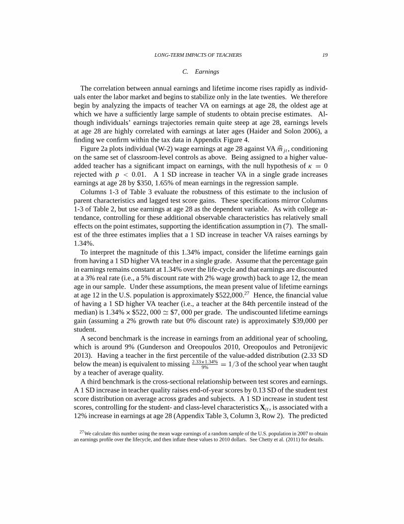
Figure 2a plots individual (W-2) wage earnings at age 28 against VA m j t , conditioning

on the same set of classroom-level controls as above. Being assigned to a higher value-

added teacher has a significant impact on earnings, with the null hypothesis of κ = 0

rejected with p < 0.01. A 1 SD increase in teacher VA in a single grade increases

earnings at age 28 by $350, 1.65% of mean earnings in the regression sample.

Columns 1-3 of Table 3 evaluate the robustness of this estimate to the inclusion of

parent characteristics and lagged test score gains. These specifications mirror Columns

1-3 of Table 2, but use earnings at age 28 as the dependent variable. As with college at-

tendance, controlling for these additional observable characteristics has relatively small

effects on the point estimates, supporting the identification assumption in (7). The small-

est of the three estimates implies that a 1 SD increase in teacher VA raises earnings by

1.34%.

To interpret the magnitude of this 1.34% impact, consider the lifetime earnings gain

from having a 1 SD higher VA teacher in a single grade. Assume that the percentage gain

in earnings remains constant at 1.34% over the life-cycle and that earnings are discounted

at a 3% real rate (i.e., a 5% discount rate with 2% wage growth) back to age 12, the mean

age in our sample. Under these assumptions, the mean present value of lifetime earnings

at age 12 in the U.S. population is approximately $522,000.27 Hence, the financial value

of having a 1 SD higher VA teacher (i.e., a teacher at the 84th percentile instead of the

median) is 1.34%×$522, 000 ' $7, 000 per grade. The undiscounted lifetime earnings

gain (assuming a 2% growth rate but 0% discount rate) is approximately $39,000 per

student.

A second benchmark is the increase in earnings from an additional year of schooling,

which is around 9% (Gunderson and Oreopoulos 2010, Oreopoulos and Petronijevic

2013). Having a teacher in the first percentile of the value-added distribution (2.33 SD

below the mean) is equivalent to missing 2.33×1.34%9%

= 1/3 of the school year when taught

by a teacher of average quality.

A third benchmark is the cross-sectional relationship between test scores and earnings.

A 1 SD increase in teacher quality raises end-of-year scores by 0.13 SD of the student test

score distribution on average across grades and subjects. A 1 SD increase in student test

scores, controlling for the student- and class-level characteristics Xi t , is associated with a

12% increase in earnings at age 28 (Appendix Table 3, Column 3, Row 2). The predicted

27We calculate this number using the mean wage earnings of a random sample of the U.S. population in 2007 to obtain

an earnings profile over the lifecycle, and then inflate these values to 2010 dollars. See Chetty et al. (2011) for details.


impact of a 1 SD increase in teacher VA on earnings is therefore 0.13× 12% = 1.55%,

similar to the observed impact of 1.34%.

Extensive Margin Responses and Other Sources of Income. The increase in wage

earnings comes from a combination of extensive and intensive margin responses. In

Column 4 of Table 3, we regress an indicator for having positive W-2 wage earnings on

teacher VA using the same specification as in Column 1. A 1 SD increase in teacher

VA raises the probability of working by 0.38%. If the marginal entrant into the labor

market were to take a job that paid the mean earnings level in the sample ($21,256),

this extensive margin response would raise mean earnings by $81. Since the marginal

entrant most likely has lower earnings than the mean, this implies that the extensive

margin accounts for at most 81/350 = 23% of the total earnings increase due to better

teachers.

Column 5 of Table 3 replicates the baseline specification in Column 1 using total in-

come (as defined in Section II) instead of wage earnings. Reassuringly, the point esti-

mate of teachers’ impacts changes relatively little with this broader income definition,

which includes self-employment and other sources of income. We therefore use wage

earnings – which provides an individual rather than household measure of earnings and

is unaffected by the endogeneity of filing – for the remainder of our analysis.

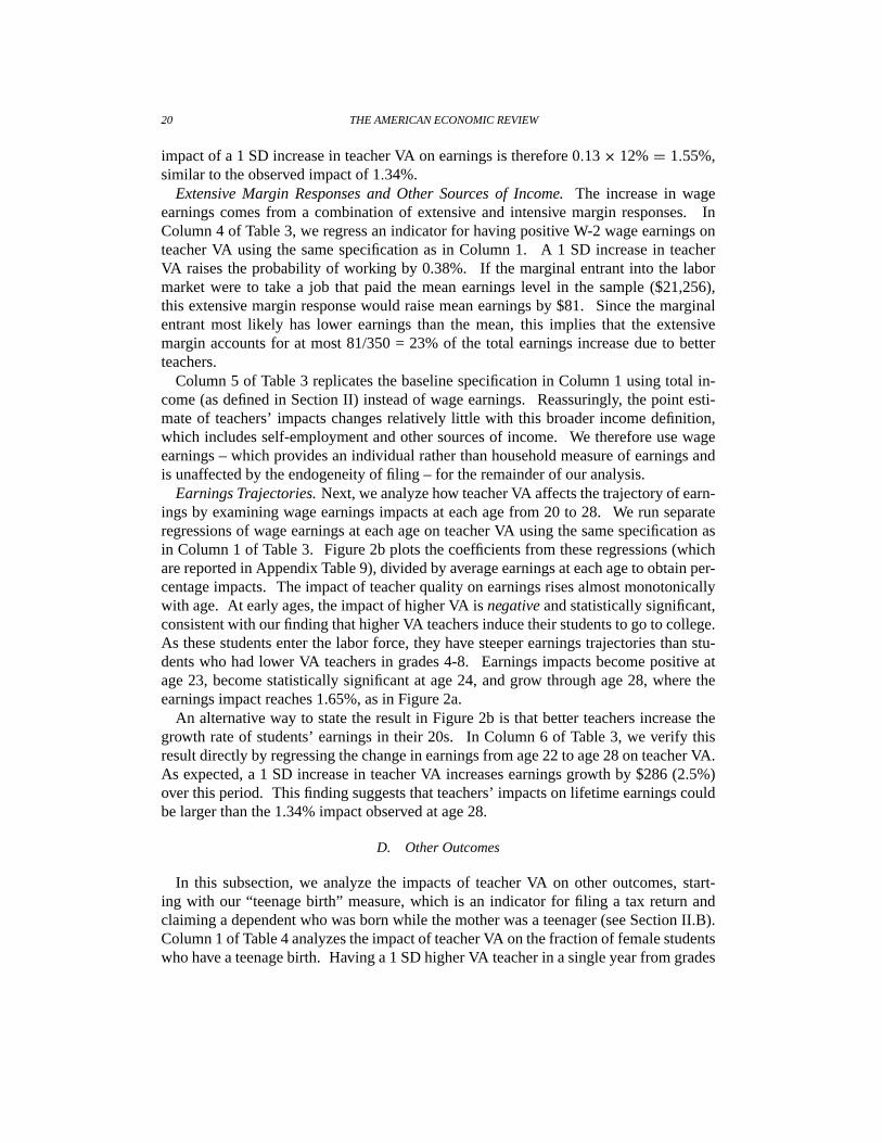
Earnings Trajectories. Next, we analyze how teacher VA affects the trajectory of earn-

ings by examining wage earnings impacts at each age from 20 to 28. We run separate

regressions of wage earnings at each age on teacher VA using the same specification as

in Column 1 of Table 3. Figure 2b plots the coefficients from these regressions (which

are reported in Appendix Table 9), divided by average earnings at each age to obtain per-

centage impacts. The impact of teacher quality on earnings rises almost monotonically

with age. At early ages, the impact of higher VA is negative and statistically significant,

consistent with our finding that higher VA teachers induce their students to go to college.

As these students enter the labor force, they have steeper earnings trajectories than stu-

dents who had lower VA teachers in grades 4-8. Earnings impacts become positive at

age 23, become statistically significant at age 24, and grow through age 28, where the

earnings impact reaches 1.65%, as in Figure 2a.

An alternative way to state the result in Figure 2b is that better teachers increase the

growth rate of students’ earnings in their 20s. In Column 6 of Table 3, we verify this

result directly by regressing the change in earnings from age 22 to age 28 on teacher VA.

As expected, a 1 SD increase in teacher VA increases earnings growth by $286 (2.5%)

over this period. This finding suggests that teachers’ impacts on lifetime earnings could

be larger than the 1.34% impact observed at age 28.

D. Other Outcomes

In this subsection, we analyze the impacts of teacher VA on other outcomes, start-

ing with our “teenage birth” measure, which is an indicator for filing a tax return and

claiming a dependent who was born while the mother was a teenager (see Section II.B).

Column 1 of Table 4 analyzes the impact of teacher VA on the fraction of female students

who have a teenage birth. Having a 1 SD higher VA teacher in a single year from grades


4 to 8 reduces the probability of a teen birth by 0.61 percentage points, a reduction of

roughly 4.6%, as shown in Figure 3a. This impact is similar to the raw cross-sectional

correlation between scores and teenage births (Appendix Table 3), echoing our results

on earnings and college attendance.

Column 2 of Table 4 analyzes the impact of teacher VA on the socio-economic status

of the neighborhood in which students live at age 28, measured by the percent of college

graduates living in that neighborhood. A 1 SD increase in teacher VA raises neigh-

borhood SES by 0.25 percentage points (1.8% of the mean) by this metric, as shown in

Figure 3b. Column 3 of Table 4 shows that a 1 SD increase in teacher VA increases the

likelihood of saving money in a 401(k) at age 28 by 0.55 percentage points (or 2.8% of

the mean), as shown in Figure 3c.

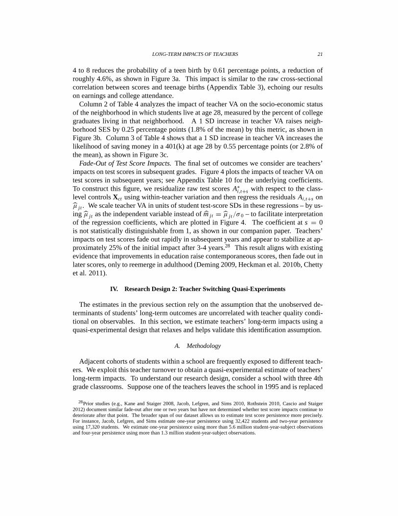
Fade-Out of Test Score Impacts. The final set of outcomes we consider are teachers’

impacts on test scores in subsequent grades. Figure 4 plots the impacts of teacher VA on

test scores in subsequent years; see Appendix Table 10 for the underlying coefficients.

To construct this figure, we residualize raw test scores A∗i,t+s with respect to the class-

level controls Xct using within-teacher variation and then regress the residuals Ai,t+s on

µ j t . We scale teacher VA in units of student test-score SDs in these regressions – by us-

ing µ j t as the independent variable instead of m j t = µ j t/σ 0 – to facilitate interpretation

of the regression coefficients, which are plotted in Figure 4. The coefficient at s = 0

is not statistically distinguishable from 1, as shown in our companion paper. Teachers’

impacts on test scores fade out rapidly in subsequent years and appear to stabilize at ap-

proximately 25% of the initial impact after 3-4 years.28 This result aligns with existing

evidence that improvements in education raise contemporaneous scores, then fade out in

later scores, only to reemerge in adulthood (Deming 2009, Heckman et al. 2010b, Chetty

et al. 2011).

IV. Research Design 2: Teacher Switching Quasi-Experiments

The estimates in the previous section rely on the assumption that the unobserved de-

terminants of students’ long-term outcomes are uncorrelated with teacher quality condi-

tional on observables. In this section, we estimate teachers’ long-term impacts using a

quasi-experimental design that relaxes and helps validate this identification assumption.

A. Methodology

Adjacent cohorts of students within a school are frequently exposed to different teach-

ers. We exploit this teacher turnover to obtain a quasi-experimental estimate of teachers’

long-term impacts. To understand our research design, consider a school with three 4th

grade classrooms. Suppose one of the teachers leaves the school in 1995 and is replaced

28Prior studies (e.g., Kane and Staiger 2008, Jacob, Lefgren, and Sims 2010, Rothstein 2010, Cascio and Staiger

2012) document similar fade-out after one or two years but have not determined whether test score impacts continue to

deteriorate after that point. The broader span of our dataset allows us to estimate test score persistence more precisely.

For instance, Jacob, Lefgren, and Sims estimate one-year persistence using 32,422 students and two-year persistence

using 17,320 students. We estimate one-year persistence using more than 5.6 million student-year-subject observations

and four-year persistence using more than 1.3 million student-year-subject observations.


by a teacher whose VA estimate is 0.3 higher, so that the mean test-score VA of the

teaching staff rises by 0.3/3 = 0.1. If the distribution of unobserved determinants of

students’ long-term outcomes does not change between 1994 and 1995, the change in

mean college attendance rates between the 1994 and 1995 cohorts of students will reveal

the impact of a 0.1 improvement in 4th grade teachers’ test-score VA. More generally,

we can estimate teachers’ long-term impacts by comparing the change in mean student

outcomes across cohorts to the change in mean VA driven by teacher turnover provided

that student quality is stable over time.

To formalize this approach, let m−{t,t−1}j t denote the test-score VA estimate for teacher

j in school year t constructed as in our companion paper using data from all years except

t − 1 and t . Similarly, let m−{t,t−1}j,t−1 denote the VA estimate for teacher j in school year

t−1 based on data from all years except t−1 and t . Let Qsgt denote the student-weighted

mean of m−{t,t−1}j t across teachers in school s in grade g, which is the average estimated

quality of teachers in a given school-grade-year cell; define Qsg,t−1 analogously.29 Let

1Qsgt = Qsgt−Qsg,t−1 denote the change in mean teacher value-added from year t−1 to

year t in grade g in school s. Define mean changes in student outcome residuals 1Ysgt

analogously. Note that because we exclude both years t and t − 1 when estimating

VA, the variation in 1Qsgt is driven purely by changes in the teaching staff and not by

changes in teachers’ VA estimates.30 As above, this leave-out technique ensures that

changes in1Ysgt are not spuriously correlated with1Qsgt due to estimation error in VA.

We estimate teachers’ long-term impacts by regressing changes in mean outcomes

across cohorts on changes in mean test-score VA:

(9) 1Ysgt = α + κ1Qsgt +1η′sgt

Note that this specification is the same as the quasi-experimental specification we used to

estimate the degree of bias in VA estimates in our companion paper, except that we use

long-term outcomes as the dependent variable instead of test scores. The coefficient in

(9) identifies the effect of a 1 SD improvement in teacher quality as defined in (6) under

the following assumption.

Assumption 3 [Teacher Switching as a Quasi-Experiment] Changes in teacher quality

across cohorts within a school-grade are orthogonal to changes in other determinants of

student outcomes 1η′sgt across cohorts:

(10) Cov(1Qsgt ,1η

′sgt

)= 0.

29In our baseline specifications, we impute teacher VA as the sample mean (0) for students for whom we have no

leave-out-year VA estimate m−{t,t−1}j t

, either because we have no teacher information or because the teacher did not

teach in the district outside of years {t − 1, t}. We show below that we obtain similar results when restricting to the

subset of school-grade-subject-year cells with no missing data on teacher VA. See Section V of our companion paper for

additional discussion on the effects of this imputation.30Part of the variation in 1Qsgt comes from drift. Even for a given teacher, predicted VA will change because our

forecast of VA varies across years. Because the degree of drift is small across a single year, drift accounts for 5.5% of the

variance in 1Qsgt . As a result, isolating the variation due purely to teacher switching using an instrumental variables

specification yields very similar results (not reported).


This assumption could potentially be violated by endogenous student or teacher sorting.

In practice, student sorting at an annual frequency is minimal because of the costs of

changing schools. During the period we study, most students would have to move to a

different neighborhood to switch schools, which families would be unlikely to do simply

because a single teacher leaves or enters a given grade. While endogenous teacher

sorting is plausible over long horizons, the sharp changes we analyze are likely driven by

idiosyncratic shocks such as changes in staffing needs, maternity leaves, or the relocation

of spouses. Moreover, in our first paper, we present direct evidence supporting (10) by

showing that both prior scores and contemporaneous scores in the other subject (e.g.,

English) are uncorrelated with changes in mean teacher quality in a given subject (e.g.,

math). We also present additional evidence supporting (10) below.

If observable characteristics Xi t are also orthogonal to changes in teacher quality

across cohorts (i.e., satisfy Assumption 3), we can implement (9) simply by regress-

ing the change in raw outcomes 1Y ∗sgt on 1Qsgt . We therefore begin with regressions

of1Y ∗sgt on1Qsgt and then confirm that changes in observable characteristics Xi t across

cohorts are uncorrelated with 1Qsgt .

B. Results

Figure 5a presents a binned scatter plot of changes in mean college attendance rates

1Y ∗sgt against changes in mean teacher value-added 1Qsgt across cohorts. We include

year fixed effects (demeaning both the x and y variables by school year), so that the esti-

mate is identified purely from differential changes in teacher value-added across school-

grade-subject cells over time. The corresponding regression coefficient, which is based

on estimating (9) with year fixed effects but no other controls, is reported in Column 1

of Table 5a.

Changes in the quality of the teaching staff have significant impacts on changes in

college attendance rates across consecutive cohorts of students in a school-grade-subject

cell. The null hypothesis that κ = 0 is rejected with p < 0.01. The point estimate

implies that a 1 SD improvement in teacher quality raises college attendance rates by

0.86 percentage points, with a standard error of 0.23. This estimate is very similar to the

estimates of 0.71-0.82 percentage points obtained from the first research design in Table

2. However, the quasi-experimental estimate is much less precise because it exploits

less variation.

This analysis identifies teachers’ causal impacts provided that (10) holds. One natural

concern is that improvements in teacher quality may be correlated with other improve-

ments in a school – such as better resources in other dimensions – that also contribute to

students’ long-term success and thus lead us to overstate teachers’ true impacts. To ad-

dress this concern, Column 2 of Table 5a replicates the baseline specification in Column

1 including school by year fixed effects instead of just year effects. In this specification,

the only source of identifying variation comes from differential changes in teacher qual-

ity across subjects and grades within a school in a given year. The coefficient on 1Qsgt

changes very little relative to the baseline estimate that pools all sources of variation.

Column 3 further accounts for secular trends in subject- or grade-specific quality by con-


trolling for the change in mean teacher VA in the prior and subsequent year as well as

cubics in the change in prior-year mean own-subject and other-subject scores across co-

horts. Controlling for these variables has little impact on the estimate. This result shows

that fluctuations in teacher quality relative to trend in specific grades generate significant

changes in the affected students’ college attendance rates.

In the preceding specifications, we imputed the sample mean of VA (0) for class-

rooms for which we could not calculate actual VA. This generates downward bias in our

estimates because we mismeasure the change in teacher quality 1Qsgt across cohorts.

Column 4 of Table 5a replicates Column 2, limiting the sample to school-grade-subject-

year cells in which we can calculate the leave-two-year-out mean for all teachers in the

current and preceding year. As expected, the point estimate of a one SD increase in

teacher quality increases, but the confidence interval is significantly wider because the

sample size is considerably smaller.

Finally, we further evaluate (10) using a series of placebo tests. In Column 5 on

Table 5a, we replicate Column 2, replacing the change in actual college attendance with

the change in predicted college attendance based on parent characteristics. We predict

college attendance using an OLS regression of Y ∗i t on the same five parent characteristics

P∗i t used in Section III.B, with no other control variables. Changes in mean teacher

VA have no effect on predicted college attendance rates, supporting the assumption that

changes in the quality of the teaching staff are unrelated to changes in student quality at

an annual level.

In Figure 6a, we present an alternative set of placebo tests based on the sharp timing of

the change in teacher quality. To construct this figure, we replicate the specification in

Column 1 but include changes in mean teacher VA for the four preceding and subsequent

cohorts as placebo effects (as well as year fixed effects):

(11) 1Y ∗sgt = αt +4∑

n=−4

κn1Qsg,t+n + ϕt

Figure 6a plots the vector of coefficients κ = (κ−4, ..., κ0, ..., κ4), which represent the

impacts of changes in the quality of teaching staff at different horizons on changes in

college attendance rates at time 0. As one would expect, κ0 is positive and highly sig-

nificant while all the other coefficients are near 0 and statistically insignificant. That

is, contemporaneous changes in teacher quality have significant effects on college atten-

dance rates, but past or future changes have no impact, as they do not directly affect the

current cohort of students. The placebo tests in Figure 6a strongly support the view that

the changes in teacher VA have causal effects on college attendance rates.31

31In Figure 3 of our companion paper, we directly use event studies around the entry and exit of teachers in the

top and bottom 5% to demonstrate the impacts of VA on test scores. We do not have adequate power to identify the

impacts of these exceptional teachers on college attendance using such event studies. In the cross-cohort regression that

pools all teaching staff changes, the t-statistic for college attendance is 3.78 (Column 1 of Table 5a in this paper). The

corresponding t-statistic for test scores is 34.0 (Column 2 of Table 5 of the first paper). We have much less power here

both because the college attendance is only observed for the older half of our sample and because college is a much

noisier outcome than end-of-grade test scores.


Figures 5b and 6b and Table 5b replicate the preceding analysis using the earnings-

based index of college quality as the outcome. We find that improvements in teachers’

test score VA across cohorts lead to sharp changes in the quality of colleges that students

attend across all of the specifications. The point estimate in the baseline specification

(Column 1) implies that a 1 SD improvement in teacher VA raises college quality by

$197 (s.e. = $60), which is not statistically distinguishable from the estimates of $266-

$299 obtained using the first research design. We find no evidence that predicted college

quality based on parent characteristics is correlated with changes in teacher quality. In

addition, changes in teacher VA again affect college quality in the year of the change

rather than in preceding or subsequent years, as shown in Figure 6b.

We used specifications analogous to those in Table 5 to investigate the impacts of

teaching quality on other outcomes, including earnings at age 28. Unfortunately, our

sample size for earnings at age 28 is roughly 1/7th the size of the sample available to

study college attendance at age 20. This is both because we have fewer cohorts of

students who are currently old enough to be observed at age 28 in the tax data and

because we have data on teacher assignments for much fewer schools in the very early

years of our school district data. Because of the considerably smaller sample, we obtain

very imprecise and fragile estimates of the impacts of teacher quality on earnings using

the quasi-experimental design.32 Hence, we are forced to rely on estimates from the

cross-class design in Table 3 to gauge earnings impacts. However, given that the cross-

class and quasi-experimental designs yield very similar estimates of teachers’ impacts

on test scores, college attendance, and college quality, we expect the cross-class design

to yield unbiased estimates of earnings impacts as well.

V. Heterogeneity of Teachers’ Impacts

In this section, we analyze whether teachers’ impacts vary across demographic groups,

subjects, and grades. Because analyzing subgroup heterogeneity requires considerable

statistical precision, we use the first research design – comparisons across classrooms

conditional on observables – which as noted above relies on a stronger identification as-

sumption but is bolstered by generating results that are similar to the quasi-experimental

design in the full sample. We estimate impacts on college quality at age 20 (rather than

earnings at age 28) to maximize precision and obtain a quantitative metric based on pro-

jected earnings gains.

A. Demographic Groups

In Panel A of Table 6, we study the heterogeneity of teachers’ impacts across demo-

graphic subgroups. Each value reported in the first row of the table is a coefficient esti-

mate from a separate regression of college quality on teacher VA conditional on controls.

To be conservative, we include both student characteristics Xct and parent characteristics

32For instance, estimating the specification in Column 1 of Table 5 with earnings at age 28 as the dependent variable

yields a confidence interval of (-$581,$665), which contains both 0 and values nearly twice as large as the estimated

earnings impacts based on our first research design.


P∗ct in the control vector throughout this section and estimate specifications analogous to

Column 5 of Table 2 on various subsamples. Columns 1 and 2 consider heterogeneity by

gender. Columns 3 and 4 consider heterogeneity by parental income, dividing students

into groups above and below the median level of parent income in the sample. Columns

5 and 6 split the sample into minority and non-minority students.

Two lessons emerge from Table 6a. First, the point estimates of the impacts of teacher

VA are larger for females than males, although we cannot reject equality of the impacts

(p = 0.102). Second, the impacts are larger for higher-income and non-minority house-

holds in absolute terms. For instance, a 1 SD increase in VA raises college quality by

$190 for children whose parents have below-median income, compared with $380 for

those whose parents have above-median income. However, the impacts are more similar

as a percentage of mean college quality: 0.80% for low-income students vs. 1.25% for

high-income students.

The larger absolute impact for high socioeconomic students could be driven by two

channels: a given increase in teacher VA could have larger impacts on the test scores of

high SES students or a given increase in scores could have larger long-term impacts. The

second row of coefficient estimates of Table 6a shows that a 1 SD increase in teacher VA

raises test scores by approximately 0.13 SD on average in all the subgroups, consistent

with the findings of Lockwood and McCaffrey (2009). In contrast, the cross-sectional

correlation between scores and college quality is significantly larger for higher SES stu-

dents (Appendix Table 5). Although not conclusive, these findings suggest that the

heterogeneity in teachers’ long term impacts is driven by the second mechanism, namely

that high SES students benefit more from test score gains.33 Overall, the heterogeneity

in treatment effects on college quality suggests that teacher quality – at least as measured

by test-score VA – is complementary to family inputs and resources. This result implies

that higher income families should be willing to pay more for high VA teachers.

B. Subjects: Math vs. English

Panel B of Table 6 analyzes differences in teachers’ impacts across subjects. For these

regressions, we split the sample into elementary (Columns 1-3) and middle (Columns 4-

5) schools. This distinction is important because students have the same teacher for both

subjects in elementary school but not middle school.

In Column 1, we replicate the baseline specification in Column 5 of Table 2, restricting

the sample to math classrooms in elementary school. Column 2 repeats this specification

for English. In Column 3, we include each teacher’s math and English VA together

in the same specification, reshaping the dataset to have one row for each student-year

(rather than one row per student-subject-year, as in previous regressions). Because a

given teacher’s math and English VA are highly correlated (r = 0.6), the magnitude of

the two subject-specific coefficients drops by an average of 40% when included together

33Importantly, the relationship between college quality and test scores conditional on prior characteristics Xi t is linear

throughout the test score distribution (Appendix Figure 2b). Hence, the heterogeneity is not due to non-linearities in the

relationship between scores and college outcomes but rather the fact that the same increase in scores translates to a bigger

change in college outcomes for high SES families.


in a single regression for elementary school. Intuitively, when math VA is included

by itself in elementary school, it partly picks up the effect of having better teaching in

English as well.

We find that a 1 SD increase in teacher VA in English has larger impacts on college

quality than a 1 SD improvement in teacher VA in math. This is despite the fact that the

variance of teacher effects in terms of test scores is larger in math than English. In Table

2 of our companion paper, we estimated that the standard deviation of teacher effects on

student test scores in elementary school is 0.124 in English and 0.163 in math. Using the

estimates from Column 3 of Table 6b, this implies that an English teacher who raises her

students’ test scores by 1 SD raises college quality by189/0.124

106/0.163= 2.3 times as much as a

math teacher who generates a commensurate test score gain. Hence, the returns to better

performance in English are especially large, although it is much harder for teachers to

improve students’ achievement in English (e.g., Hanushek and Rivkin 2010, Kane et al.

2013).

We find a similar pattern in middle school. In Column 4 of Table 6b, we replicate

the baseline specification for the subset of observations in math in middle school. We

control for teacher VA in English when estimating this specification by residualizing

college quality Y ∗i t with respect to the student and parent class-level control vectors Xct

and P∗i t as well as m j t in English using a regression with math teacher fixed effects as in

(3). Column 5 of Table 6b replicates the same regression for observations in English in

middle school, controlling for math teacher VA. A 1 SD improvement in English teacher

quality raises college quality by roughly twice as much as a 1 SD improvement in math

teacher quality. Even though teachers have much smaller impacts on English test scores

than math test scores, the small improvements that good teachers generate in English are

associated with substantial long-term impacts.

C. Impacts of Teachers by Grade

We estimate the impact of a 1 SD improvement in teacher quality in each grade g ∈[4, 8] on college quality (κg) by estimating the specification in Column 5 of Table 2 but

interacting m j t with grade dummies. Because the school district data system did not

cover many middle schools in the early and mid 1990s, we cannot analyze the impacts of

teachers in grades 6-8 for more than half the students who are in 4th grade before 1994.

To obtain a more balanced sample for comparisons across grades, we restrict attention to

cohorts who would have been in 4th grade during or after 1994 in this subsection.34

The series in circles in Figure 7 plots the estimates of κg, which are also reported in

Appendix Table 11. We find that teachers’ long-term impacts are large and significant

in all grades. Although the estimates in each grade have relatively wide confidence in-

tervals, there is no systematic trend in the impacts. This pattern is consistent with the

cross-sectional correlations between test scores and adult outcomes, which are also rela-

tively stable across grades (Appendix Table 6). One issue that complicates cross-grade

34Restricting the sample in the same way does not affect the conclusions above about heterogeneity across subjects or

demographic groups, because these groups are balanced across cohorts.


comparisons is that teachers spend almost the entire school day with their students in el-

ementary school (grades 4-5 as well as 6 in some schools), but only their subject period

(Math or English) in middle school (grades 7-8). If teachers’ skills are correlated across

subjects – as is the case with math and English value-added, which have a correlation of

0.6 for elementary school teachers – then a high-VA teacher should have a greater impact

on earnings in elementary school than middle school because they spend more time with

the student. Hence, the fact that high-VA math and English teachers continue to have

substantial impacts in middle school indicates that education has substantial returns well

beyond early childhood.

Tracking and Net Impacts. The reduced-form estimates of κg reported above include

the impacts of being tracked to a better teacher in subsequent grades, as discussed in

Section I. While a parent may be interested in the reduced-form impact of teacher VA

in grade g, a policy that raises teacher quality in grade g will not allow every child to get

a better teacher in grade g + 1. We now turn to identifying teachers’ net impacts κg in

each grade, holding fixed future teachers’ test-score VA.

Because we have no data after grade 8, we can only estimate teachers’ net effects

holding fixed teacher quality up to grade 8. We therefore set κ8 = κ8. We recover

κg from estimates of κg by subtracting out the impacts of future teachers on earnings

iteratively. The net impact of a 7th grade teacher is her reduced-form impact κ7 minus

her indirect impact via tracking to a better 8th grade teacher:

(12) κ7 = κ7 − ρ78κ8,

where ρ78 is the extent to which teacher VA in grade 7 increases teacher VA in grade

8 conditional on controls. If we observed each teacher’s true VA, we could estimate

ρ78 using an OLS regression that parallels (8) with the future teacher’s true VA as the

dependent variable:

(13) m j,ti (8) = α + ρ78m j,ti (7) + γ 1Xct + γ 2P∗ct + ηµct78.

Since true VA is unobserved, we substitute VA estimates m j,ti (8) for m j,ti (8) on the left

hand side of (13). This yields an attenuated estimate of ρ78 because m j,ti (8) is shrunk

toward 0 to account for estimation error (see Section I.B of our companion paper). If

all teachers taught the same number of classes and had the same number of students,

the shrinkage factor would not vary across observations. In this case, we could identify

ρ78 by using m j,ti (8) as the dependent variable in (13) and multiplying the estimate of

ρ78 by SD(m j t)/SD(m j t) = 1/SD(m j t). In the sample for which we observe col-

lege attendance, the standard deviation of teacher VA estimates is SD(m j t) = 0.61.

We therefore multiply the estimate of ρ78 and all the other tracking coefficients ρgg′ by

1/SD(m j t) = 1.63. This simple approach to correcting for the attenuation bias is an

approximation because the shrinkage factor does vary across observations. However, as

we discuss below, the magnitude of the tracking coefficients is small and hence further

adjusting for the variation in shrinkage factors is unlikely to affect our conclusions.

We estimate ρ78 in three steps. First, we residualize m j,ti (8) with respect to the controls


by regressing m j,ti (8) on Xct and P∗ct with grade 7 teacher fixed effects, as in (3). Second,

we run a univariate OLS regression of the residuals on m j,ti (7). Finally, we multiply this

coefficient by 1/SD(m j t) = 1.63 to obtain an estimate of ρ78. Using our estimate of

ρ78, we apply (12) to identify κ7 from the reduced-form estimates of κg in Figure 7.

Iterating backwards, we calculate κ6 by estimating ρ68 and ρ67 and so on until we obtain

the full set of net impacts. We show formally that this procedure recovers net impacts

κg in Appendix C.

The series in triangles in Figure 7 plots the estimates of the net impacts κg. The

differences between the net impacts and reduced-form impacts are modest: the mean

difference between κg and κg is 19.6% in grades 4-7. This is because the tracking

coefficients ρg,g′ are small. A 1 SD increase in current teacher quality typically raises

future teacher quality by about 0.05 SD or less in elementary school and by about 0.25

SD in middle school (Appendix Table 12). The greater degree of tracking in middle

school is consistent with the availability of subject-specific honors classes in grades 7

and 8.

These results suggest that the vast majority of the reduced-form impacts estimated

above reflect a teacher’s own direct impact rather than the impacts of being tracked to

better teachers in later grades. However, we caution that this approach to calculating

teachers’ net impacts has three important limitations. First, it assumes that all tracking

to future teachers occurs exclusively via teachers’ test-score VA. We allow students who

have high-VA teachers in grade g to be tracked to higher test-score VA (m j t ) teachers in

grade g+1, but not to teachers with higher earnings VA µYjt . We are forced to make this

strong assumption because we have no way to estimate teacher impacts on earnings that

are orthogonal to VA, as discussed in Section I. Second, κg does not net out potential

changes in other factors besides teachers, such as peer quality or parental inputs. Hence,

κg cannot be interpreted as the “structural” impact of teacher quality holding fixed all

other inputs in a general model of the education production function (e.g., Todd and

Wolpin 2003). Finally, our approach assumes that teacher effects are additive across

grades. We cannot identify complementarities in teacher VA across grades because our

identification strategy forces us to condition on lagged test scores, which are endogenous

to the prior teacher’s quality. It would be very useful to relax these assumptions in future

work to obtain a better understanding of how the sequence of teachers a child has affects

her outcomes in adulthood.

VI. Policy Analysis

In this section, we use our estimates to predict the potential earnings gains from se-

lecting and retaining teachers on the basis of their VA. We make four assumptions in

our calculations. First, we assume that the percentage impact of a 1 SD improvement in

teacher VA on earnings observed at age 28 is constant at b = 1.34% (Table 3, Column

2) over the lifecycle.35 Second, we ignore general equilibrium effects that may reduce

35We have inadequate precision to estimate wage earnings impacts separately by subject and grade level. We therefore

assume that a 1 SD improvement in teacher VA raises earnings by 1.34% in all subjects and grade levels in the calculations

that follow.


wage rates if all children are better educated. Third, we follow Krueger (1999) and dis-

count earnings gains at a 3% real annual rate (consistent with a 5% discount rate and 2%

wage growth) back to age 12, the average age in our sample. Under this assumption,

the present value of earnings at age 12 for the average individual in the U.S. population

is $522, 000 in 2010 dollars, as noted above. Finally, we assume that teacher VA m j t is

normally distributed.

To quantify the value of improving teacher quality, we evaluate Hanushek’s (2009,

2011) proposal to replace teachers whose VA ratings are in the bottom 5 percent of the

distribution with teachers of average quality. To simplify exposition, we calculate these

impacts for elementary school teachers, who teach one class per day. We first calculate

the earnings gains from selecting teachers based on their true test-score VA m j t and then

calculate the gains from selecting teachers based on VA estimates m j t . Selection on true

VA is informative as a benchmark for the potential gains from improving teacher quality,

but is not a feasible policy because we only observe estimates of teacher VA in practice.

Hence, it is useful to compare the gains from policies that select teachers based on VA

estimates using a few years of performance data with the maximum attainable gain if one

were to select teachers based on true VA.

Selection on True VA. Elementary school teachers teach both math and English and

therefore have two separate VA measures on which they could be evaluated. For sim-

plicity, we assume that teachers are evaluated based purely on their VA in one subject

(say math) and VA in the other subject is ignored.36 Consider a student whose teacher’s

true math VA is 1mσ standard deviations below the mean. Replacing this teacher with

a teacher of mean quality (for a single school year) would raise the student’s expected

earnings by

(14) G = 1mσ × $522, 000× b.

Under the assumption that m j t is normally distributed, a teacher in the bottom 5% of

the true VA distribution is on average 2.063 standard deviations below the mean teacher

quality. Therefore, replacing a teacher in the bottom 5% of the VA distribution with an

average teacher generates a present value lifetime earnings gain per student of

G = $522, 000× 2.063× 1.34% = $14, 500.

For a class of average size (28.2), the total NPV earnings impact from this replacement is

GC = $407, 000. The undiscounted cumulative lifetime earnings gains from deselection

are 5.5 times larger than these present value gains ($80,000 per student and $2.25 million

per classroom), as shown in Appendix Table 13.37 These simple calculations show that

36School districts typically average math and English VA ratings to calculate a single measure of teacher performance

in elementary schools (e.g., District of Columbia Public Schools 2012). In Appendix D, we show that the gains from

evaluating teachers based on mean math and English VA are only 12% larger than the gains from using information based

on only one subject because math and English VA estimates are highly correlated. Therefore, the results we report below

slightly underestimate the true gains from selection on mean VA.37These calculations do not account for the fact that deselected teachers may be replaced by rookie teachers, who

have lower VA. In our sample, mean test score residuals for students taught by first-year teachers are on average 0.05 SD


the potential gains from improving the quality of teaching – whether using selection

based on VA, teacher training, or other policies – are quite large.38

Selection on Estimated VA. In practice, we can only select teachers on the basis of

estimated VA m j t . This reduces the gains from selection for two reasons: (1) estimation

error in VA and (2) drift in teacher quality over time. To quantify the impact of these

realities, suppose we use test score data from years t = 1, ..., n to estimate teacher VA

in school year n + 1. The gain in year n + 1 from replacing the bottom 5% of teachers

based on VA estimated using the preceding n years of data is

(15) G(n) = −E[m j,n+1 | m j,n+1 < F−1

m j,n+1(0.05)

]× $522, 000× b,

where E[m j,n+1 | m j,n+1 < F−1

m j,n+1(0.05)

]denotes the expected value of m j,n+1 con-

ditional on the teacher’s estimated VA falling below the 5th percentile. We calculate

this expected value separately for math and English using Monte Carlo simulations as

described in Appendix D.39

Figure 8a plots the mean gain per classroom GC(n) = 28.2 × G(n), averaging over

math and English, for n = 1, ..., 10. The values underlying this figure are reported

in Appendix Table 13. The gain from deselecting teachers based on true VA, GC =$407, 000, is shown by the horizontal line in the figure. The gains from deselecting

teachers based on estimated VA are significantly smaller because of noise in VA estimates

and drift in teacher quality.40 With one year of data, the expected gain per class is

$226,000, 56% of the gain from selecting on true VA. The gains grow fairly rapidly with

more data in the first 3 years, but the marginal value of additional information is small.

With three years of test score data, the gain is $266,000, but the gain increases to only

$279,000 after 10 years. After three years, waiting for one more year would increase the

gain by $4,000 but has an expected cost of $266,000. The marginal gains from obtaining

one more year of data are outweighed by the expected cost of having a low VA teacher

on the staff even after the first year (Staiger and Rockoff 2010). Adding data from prior

classes yields relatively little information about current teacher quality both because of

decreasing returns to additional observations and drift.41

lower (in units of standardized student test scores) than those taught by more experienced teachers. Given that the median

teacher remains in the district for approximately 10 years, accounting for the effect of inexperience in the first year would

reduce the expected benefits of deselection over a typical horizon by0.05/10

2.063×σ(m j t )= 2%, where σ(m j t ) = 0.14 is the

mean SD of teacher effects across elementary school subjects in our data (see Table 2 of the first paper).38Moreover, these calculations do not include the non-monetary returns to a better education (Oreopoulos and Salvanes

2010), such as lower teenage birth rates.39Without drift, the formula in (15) reduces to r(n)1/2 × 2.063 × $522, 000 × b, where r(n) denotes the reliability

of the VA estimate using n years of data, which is straightforward to calculate analytically. The original working paper

version of our study (Chetty, Friedman, and Rockoff 2011b) used this version of the formula and an estimate of b based

on a model that did not account for drift.40In Panel B of Appendix Table 13, we distinguish these two factors by eliminating estimation error and predicting

current VA based on past VA instead of past scores. Without estimation error, GC (1) = $340, 000. Hence, drift and

estimation error each account for roughly half of the difference between GC (1) and GC .41We also replicated the simulations using VA estimates that do not account for drift. When the estimation window n

is short, drift has little impact on the weights placed on test scores across years. As a result, drift-unadjusted measures

yield rankings of teacher quality that are very highly correlated with our measures and thus produce similar gains. For


Drift in Quality over Subsequent School Years. The values in Figure 8a reflect the

gains in the first year after the deselection of teachers, based on m j,n+1 in school year

n + 1. Now consider the impacts of such a policy on the earnings of students in a

subsequent school year n + m:

G(m, n) = −E[m j,n+m | m j,n+1 < F−1

m j,n+1(0.05)

]× $522, 000× b,

where E[m j,n+m | m j,n+1 < F−1

m j,n+1(0.05)

]denotes the mean VA of teachers in year n+

m conditional on having estimated VA in year n + 1 below the 5th percentile.

The lower series in Figure 8b plots GC(m, 3) = 28.2×G(m, 3), the gains per class in

school year m from deselecting teachers based on their estimated VA for year 4 (m j,4),

constructed using the first 3 years of data. The first point in this series coincides with

the value of $266,000 in Figure 8a reported for n = 3. Because teacher quality drifts

over time, the gains fall in subsequent school years, as some of the teachers who were

deselected based on their predicted VA in school year n would have reverted toward the

mean in subsequent years. Deselection based on VA estimates at the end of year 3

generates an average gain of $184,000 per classroom per year over the subsequent 10

years, the median survival time in the district for teachers who have taught for 3 years.

The upper series in Figure 8b plots the analogous gains when teachers are deselected

based on their true VA m j,4 in year 4 instead of their estimated VA m j,4. The first point

in this series coincides with the maximum attainable gain of $407,000 shown in Figure

8a. The gains again diminish over time because of drift in teacher quality. The average

present value gain from deselection based on true VA over the subsequent ten years is

approximately $250,000 per classroom. This corresponds to an undiscounted lifetime

earnings gain per classroom of students of approximately $1.4 million.

The reason that estimation error and drift do not heavily erode the gains from deselec-

tion of low VA teachers is that very few of the teachers rated in the bottom 5% turn out

to be high-VA teachers. For example, among math teachers in Elementary school, 3.2%

of the teachers whose estimated VA based on 3 years of test score data (m j,4) is in the

bottom 5% have true VA m j,4 above the median. Nevertheless, because VA estimates are

not perfect predictors of m j t , there is still substantial room to use other measures – such

as principal evaluations or student surveys – to complement VA estimates and improve

predictions of teacher quality.42

Costs of Teacher Selection. The calculations above do not account for the costs associ-

ated with a policy that deselects teachers with the lowest performance ratings. First, they

ignore downstream costs that may be required to generate earnings gains, most notably

the cost associated with higher college attendance rates. Second, and more importantly,

they ignore the fact that teachers need to be compensated for the added employment risk

instance, selection based on 3 years of data using VA estimates that do not adjust for drift yields gains that are 98%

as large as those reported above. Hence, while accounting for drift is important for evaluating out-of-sample forecasts

accurately, it may not be critical for practical policy applications for VA.42Of course, these other measures will also be affected by drift and estimation error. For instance, classroom obser-

vations have significant noise and may capture transitory fluctuations in teacher quality (Kane et al. 2013).


they face from such an evaluation system. Rothstein (2013) estimates the latter cost

using a structural model of the labor market for teachers. Rothstein estimates that a

policy that fires teachers if their estimated VA after 3 years falls below the 5th percentile

would require a mean salary increase of 1.4% to equilibrate the teacher labor market.43

In our sample, mean teacher salaries were approximately $50,000, implying that annual

salaries would have to be raised by approximately $700 for all teachers to compensate

them for the additional risk. Based on our calculations above, the deselection policy

would generate NPV gains of $184,000 per teacher deselected, or $9,250 for all teach-

ers on average (because only one out of twenty teachers would actually be deselected).

Hence, the estimated gains from this policy are more than 10 times larger than the costs.

Together with the preceding results, Rothstein’s (2013) findings imply that deselecting

low VA teachers could be a very cost effective policy if the signal quality of VA does not

fall substantially when used for personnel evaluation.44

Retention of High VA Teachers. An alternative approach to improving teacher quality

that may impose lower costs on teachers is to increase the retention of high-VA teachers

by paying them bonuses. Using Monte Carlo simulations analogous to those above, we

estimate that retaining a teacher at the 95th percentile of the estimated VA distribution

(using 3 years of data) for an extra year would yield present value earnings gains in the

subsequent school year of $522, 000×28.2×1.34%×E[m j,n+1|m j,n+1 = F−1

m j,n+1(0.95)

]=

$212, 000. In our data, roughly 9% of teachers in their third year do not return to the

school district for a fourth year. The attrition rate is unrelated to teacher VA, consistent

with the findings of Boyd et al. (2008). Clotfelter et al. (2008) estimate that a $1,800

bonus payment in North Carolina reduces attrition rates by 17%. Based on these esti-

mates, a one time bonus payment of $1,800 to high-VA teachers who return for a fourth

year would increase retention rates in the next year by 1.5 percentage points and gener-

ate an average benefit of $3,180. The expected benefit of offering a bonus to even an

excellent (95th percentile) teacher is only modestly larger than the cost because one must

pay bonuses to (100− 9)/1.5 ≈ 60 additional teachers for every extra teacher retained.

Replacing ineffective teachers is more cost-effective than attempting to retain high

VA teachers because most teachers stay for the following school year and are relatively

inelastic to salary increases. Of course, increasing the salaries of high VA teachers

could attract more talented individuals into teaching to begin with or increase teacher

effort. The preceding calculations do not account for these effects.

VII. Conclusion

Our first paper (Chetty, Friedman, and Rockoff 2014) showed that existing test-score

value-added measures are a good proxy for a teacher’s ability to raise students’ test

43In the working paper version of his study, Rothstein calculates the wage gains needed to compensate teachers for a

policy that deselects teachers below the 20th percentile after 2 years. Jesse Rothstein kindly provided the corresponding

estimates for the policy analyzed here in personal correspondence.44Even if there is erosion, as long as the signal quality of VA is a continuous function of its weight in evaluation

decisions, one would optimally place non-zero weight on VA, because the net gains would fall from the initial level of

$184,000 in proportion to the weight on VA.


scores. This paper has shown that the same VA measures are also an informative proxy

for teachers’ long-term impacts. Although these findings are encouraging for the use

of value-added metrics, two important issues must be resolved before one can determine

how VA should be used for policy.

First, using VA measures to evaluate teachers could induce responses such as teaching

to the test or cheating, eroding the signal in VA measures (e.g., Jacob 2005, Neal and

Schanzenbach 2010).45 One can estimate the magnitude of such effects by replicating

the analysis in this paper in a district that evaluates teachers based on their VA. If behav-

ioral responses substantially reduce the signal quality of VA, policy makers may need to

develop metrics that are more robust to such responses, as in Barlevy and Neal (2012).

For instance, districts may also be able to use data on the persistence of test score gains

to identify test manipulation and develop a more robust estimate of teacher quality, as in

Jacob and Levitt (2003).

Second, one should compare the long-term impacts of evaluating teachers on the basis

of VA to other metrics, such as principal evaluations or classroom observation. One can

adapt the methods developed in this paper to evaluate these other measures of teacher

quality. When a teacher who is rated highly by principals enters a school, do sub-

sequent cohorts of students have higher college attendance rates and earnings? What

fraction of a teacher’s long-term impact is captured by test-score VA vs. other measures

of teacher quality? By answering these questions, one could ultimately estimate the

optimal weighting of available metrics to identify teachers who are most successful in

improving students’ long-term outcomes.

More generally, there are many aspects of teachers’ long-term impacts that remain to

be explored and would be helpful in designing education policy. For example, in this

paper we only identified the impact of a single teacher on long-term outcomes. Are

teachers’ impacts additive over time? Do good teachers complement or substitute for

each other across years? Similarly, it would be useful to go beyond the mean treatment

effects that we have estimated here and determine whether some teachers are especially

effective in improving lower-tail outcomes or producing stars.

Whether or not VA is ultimately used as a policy tool, our results show that parents

should place great value on having their child in the classroom of a high value-added

teacher. Consider a teacher whose true VA is 1 SD above the mean who is contemplating

leaving a school. Each child would gain approximately $39,000 in total (undiscounted)

lifetime earnings from having this teacher instead of the median teacher. With an annual

discount rate of 5%, the parents of a classroom of average size should be willing to pay

this teacher $200,000 ($7,000 per parent) to stay and teach their children during the next

school year. Hence, the most important lesson of this study is that improving the quality

of teaching – whether via the use of value-added metrics or other policy levers – is likely

to have substantial economic and social benefits.

45As we noted above, even in the low-stakes regime we study, some unusually high VA teachers have test score impacts

consistent with test manipulation. If such behavior becomes more prevalent when VA is used to evaluate teachers, the

predictive content of VA as a measure of true teacher quality could be compromised.


REFERENCES

Aaronson, Daniel, Lisa Barrow, and William Sander. 2007. “Teachers and Student

Achievement in Chicago Public High Schools.” Journal of Labor Economics 24(1):

95-135.

Baker, Eva L., Paul E. Barton, Linda Darling-Hammond, Edward Haertel, Helen F.

Ladd, Robert L. Linn, Diane Ravitch, Richard Rothstein, Richard J. Shavelson,

and Lorrie A. Shepard. 2010. “Problems with the Use of Student Test Scores to

Evaluate Teachers.” Economic Policy Institute Briefing Paper #278.

Barlevy, Gadi and Derek Neal. 2012. “Pay for Percentile.” American Economic Review

102 (5): 1805-1831.

Boyd, Donald, Pamela Grossman, Hamilton Lankford, Susanna Loeb, and James

Wyckoff. 2008. “Who Leaves? Teacher Attrition and Student Achievement.”

NBER Working Paper 14022.

Cameron, Colin A., Jonah B. Gelbach, and Douglas Miller. 2011. “Robust Inference

with Multi-way Clustering,” Journal of Business and Economic Statistics 29 (2):

238-249.

Carrell, Scott E. and James E. West. 2010. “Does Professor Quality Matter? Evidence

from Random Assignment of Students to Professors,” Journal of Political Economy

118(3): 409-432.

Cascio, Elizabeth and Douglas Staiger. 2012. “Knowledge, Tests, and Fadeout in

Educational Interventions.” NBER Working Paper 18038.

Chamberlain, Gary. 2013. “Predictive Effects of Teachers and Schools on Test Scores,

College Attendance, and Earnings.” Proceedings of the National Academy of Sci-

ences 110(43).

Chetty, Raj, John N. Friedman, Nathaniel Hilger, Emmanuel Saez, Diane Schanzen-

bach, and Danny Yagan. 2011. “How Does Your Kindergarten Classroom Af-

fect Your Earnings? Evidence from Project STAR” Quarterly Journal of Economics

16(4): 1593-1660, 2011.

Chetty, Raj, John N. Friedman, and Jonah E. Rockoff. 2011a. “New Evidence on the

Long-Term Impacts of Tax Credits.” IRS Statistics of Income White Paper.

Chetty, Raj, John N. Friedman, and Jonah E. Rockoff. 2011b. “The Long Term

Impacts of Teachers: Teacher Value-Added and Student Outcomes in Adulthood.”

NBER Working Paper 17699.

Chetty, Raj, John N. Friedman, and Jonah E. Rockoff. 2014. “Measuring the Impacts

of Teachers I: Evaluating Bias in Teacher Value-Added Estimates.” The American

Economic Review (forthcoming).

Clotfelter, Charles, Elizabeth Glennie, Helen Ladd, and Jacob Vigdor. 2008. “Would

higher salaries keep teachers in high-poverty schools? Evidence from a policy inter-

vention in North Carolina.” Journal of Public Economics 92: 1352-70.

Corcoran, Sean P. 2010. “Can Teachers be Evaluated by Their Students’ Test Scores?

Should they Be? The Use of Value-Added Measures of Teacher Effectiveness in Pol-

icy and Practice.” Report for the Annenberg Institute for School Reform, Education

Policy for Action Series.


Deming, David. 2009. “Early Childhood Intervention and Life-Cycle Development:

Evidence from Head Start.” American Economic Journal: Applied Economics 1(3):

111-134.

District of Columbia Public Schools. 2012. “IMPACT: The District of Columbia Pub-

lic Schools Effectiveness Assessment System for School-Based Personnel.”

Dynarski, Susan, Joshua M. Hyman, and Diane Whitmore Schanzenbach. 2013.

“Experimental Evidence on the Effect of Childhood Investments on Postsecondary

Attainment and Degree Completion.” Journal of Policy Analysis and Management

32(4): 692-717.

Gordon, Robert, Thomas J. Kane, and Douglas O. Staiger. 2006. “Identifying Ef-

fective Teachers Using Performance on the Job,” The Hamilton Project White Paper

2006-01.

Gunderson, Morley K. and Philip Oreopoulos. 2010. “Returns to Education in Devel-

oped Countries ”, in International Encyclopedia of Education, 3rd edition (edited

by E. Barker, M. McGaw and P. Peterson), Elsevier Publishers, USA.

Haider, Steven, and Gary Solon. 2006. “Life-cycle variation in the Association Be-

tween Current and Lifetime Earnings.” American Economic Review 96: 1308-1320.

Hanushek, Eric A. 1971. “Teacher Characteristics and Gains in Student Achievement:

Estimation Using Micro Data.” American Economic Review Papers and Proceedings

61(2): 280-88.

Hanushek, Eric A., and Steven G. Rivkin. 2010. “Generalizations About Using Value-

Added Measures of Teaching Quality.” American Economic Review Papers and Pro-

ceedings 100(2): 267-71.

Hanushek, Eric A. 2009. “Teacher Deselection.” in Creating a New Teaching Profes-

sion, ed. Dan Goldhaber and Jane Hannaway, 165–80. Washington, DC: Urban

Institute Press.

Hanushek, Eric A. 2011. “The Economic Value of Higher Teacher Quality.” Economics

of Education Review 30: 466–479.

Heckman, James J., Seong H. Moon, Rodrigo Pinto, Peter A. Savelyev, and Adam.

Yavitz. 2010a. “Analyzing Social Experiments as Implemented: A Reexamina-

tion of the Evidence from the HighScope Perry Preschool Program.” Quantitative

Economics 1(1): 1-46.

Heckman, James J., Lena Malofeeva, Rodrigo Pinto, and Peter A. Savelyev. 2010b.

“Understanding the Mechanisms Through Which an Influential Early Childhood

Program Boosted Adult Outcomes,” University of Chicago, unpublished.

Internal Revenue Service. 2010. Document 6961: Calendar Year Projections of Infor-

mation and Withholding Documents for the United States and IRS Campuses 2010-

2018, IRS Office of Research, Analysis, and Statistics, Washington, D.C.

Jackson, C. Kirabo. 2013 “Non-Cognitive Ability, Test Scores, and Teacher Quality:

Evidence from 9th Grade Teachers in North Carolina.” NBER Working Paper 18624.

Jacob, Brian A. 2005. “Accountability, Incentives and Behavior: The Impact of High-

Stakes Testing in the Chicago Public Schools.” Journal of Public Economics 89(6):

761–796.


Jacob, Brian A. and Steven D. Levitt. 2003. “Rotten Apples: An Investigation Of

The Prevalence And Predictors Of Teacher Cheating.” The Quarterly Journal of

Economics 118(3): 843-877.

Jacob, Brian A., Lars Lefgren, and David P. Sims. 2010. “The Persistence of Teacher-

Induced Learning Gains,” Journal of Human Resources, 45(4): 915-943.

Kane, Thomas J., and Douglas O. Staiger. 2008. “Estimating Teacher Impacts on

Student Achievement: An Experimental Evaluation,” NBER Working Paper No.

14607.

Kane, Thomas J., Daniel F. McCaffrey, Trey Miller, and Douglas O. Staiger. 2013.

Have We Identified Effective Teachers? Validating Measures of Effective Teaching

Using Random Assignment. Seattle, WA: Bill & Melinda Gates Foundation.

Krueger, Alan B. 1999. “Experimental Estimates of Education Production Functions.”

Quarterly Journal of Economics 114(2): 497-532.

Lockwood, J.R. and Daniel F. McCaffrey. 2009. “Exploring Student-Teacher Inter-

actions in Longitudinal Achievement Data,” Education Finance and Policy 4(4):

439-467.

Murnane, Richard J. 1975. The Impact of School Resources on the Learning of Inner

City Children. Cambridge, MA: Ballinger.

Neal, Derek A. and Diane Whitmore Schanzenbach. 2010. “Left Behind by Design:

Proficiency Counts and Test-Based Accountability,” Review of Economics and Sta-

tistics 92(2): 263-283.

Oreopoulos, Philip and Uros Petronijevic. 2013. “Making College Worth It: A Review

of Research on the Returns to Higher Education,” NBER Working Paper 19053.

Oreopoulos, Philip, and Kjell G. Salvanes. 2010. “Priceless: The Nonpecuniary Ben-

efits of Schooling.” Journal of Economic Perspectives 25(1): 159–84.

Rivkin, Steven. G., Eric. A. Hanushek, and John F. Kain. 2005. “Teachers, Schools

and Academic Achievement.” Econometrica 73: 417–458.

Rockoff, Jonah E. 2004. “The Impact of Individual Teachers on Student Achievement:

Evidence from Panel Data,” American Economic Review 94: 247-252.

Rothstein, Jesse. 2010. “Teacher Quality in Educational Production: Tracking, Decay,

and Student Achievement,” Quarterly Journal of Economics 125(1): 175-214.

Rothstein, Jesse. 2013. “Teacher Quality Policy When Supply Matters,” UC-Berkeley

mimeo.

Staiger, Douglas O., and Jonah E. Rockoff. 2010. “Searching for Effective Teachers

with Imperfect Information.” Journal of Economic Perspectives 24: 97-117.

Todd, Petra E. and Kenneth I. Wolpin. 2003. "On the Specification and Estima-

tion of the Production Function for Cognitive Achievement" The Economic Journal

113(485): F3-F33.

U.S. Census Bureau. 2010. “School Enrollment–Social and Economic Characteristics

of Students: October 2008, Detailed.” Washington, D.C.

http://www.census.gov/population/www/socdemo/school.html.


Online Appendix A: Structural Interpretation of Reduced-Form Parameters

This appendix formalizes how the reduced-form parameters we estimate should be

interpreted in a stylized dynamic model of the education production function. The model

we outline below follows previous work (e.g., Todd and Wolpin 2003), except that we

focus exclusively on the role of teachers, abstracting from other inputs to the education

production function, such as peers or parental investment.

Dynamic Model: Setup

The model is characterized by a specification for scores, a specification for earnings

(or other adult outcomes), and a rule that governs student and teacher assignment to

classrooms.

Classroom Assignment Rule. School principals assign student i in school year t to

a classroom c = c(i, t) based on observed and unobserved determinants of student

achievement. Principals then assign a teacher j to each classroom c based on class-

room and teacher characteristics. For simplicity, we assume that each teacher teaches

one class per year, as in elementary schools.

Test Scores. Let j = j (c(i, t)) denote student i’s teacher in school year t . Let µ j t

represent teacher j’s “test-score value-added” in year t .46 We scale µ j t in student test-

score SDs so that the average teacher has µ j t = 0 and the effect of a 1 unit increase in

teacher value-added on end-of-year test scores is 1. Let ti (g) denote the calendar year in

which student i reaches grade g; ti (0) denotes the year in which the student starts school

(Kindergarten). As in Section I, student i’s test score in year t , A∗i t , is

(16) A∗i t = βXi t + µ j t + εi t

where Xi t denotes observable determinants of student achievement, such as lagged test

scores and family characteristics and εi t is an idiosyncratic student-level error.

Earnings. Earnings are a function of teacher quality over all years in school, up to

grade G = 12. Let τ j t represent teacher j’s “direct earnings value-added,” i.e. the

direct impact of teacher j on earnings holding other factors fixed. We scale τ j t so that

the average teacher has τ j t = 0 and the standard deviation of τ j t is 1. We assume that a

teacher’s direct earnings value-added τ j t is linearly related to her test-score value-added

µ j t :

τ j t = φµ j t + τ⊥j t

where φ measures the relationship between earnings- and test-score VA and τ⊥j t repre-

sents the portion of a teacher’s earnings impact that is orthogonal to her test-score impact.

For a student in grade h, we model earnings Y ∗i as

(17) Y ∗i = βY X i t +

G∑g=h

γ gτ j,ti (g) + εYit

46To simplify notation, we writeµ j(i,t),t asµ j t and always denote by j the teacher who taught student i in the relevant

year t . For instance, µ j,t−s denotes the value-added in year t − s of the teacher j who taught student i in year t − s.

We adopt the same convention with τ j t below as well.


where γ g measures the effect of teacher quality in grade g on earnings. The error term

εYit reflects individual heterogeneity in earnings ability, which may be correlated with

academic ability εi t . The error εYit may also be correlated with µ j t and τ j t because the

principal may systematically sort certain types of students to certain teachers. Account-

ing for such selection is the key challenge in obtaining unbiased estimates of teachers’

causal impacts.

In the statistical model in (3), the teacher fixed effect α j =G∑

g=h

γ gτ j,ti (g) combines the

effects of the current and subsequent teachers. We show how this affects the interpreta-

tion of the reduced-form treatment effects we estimate in the next subsection.

Treatment Effects in the Dynamic Model

We define two notions of a teacher’s treatment effect on earnings: total earnings value-

added and the impact of test-score VA on earnings.

Total Earnings Value-Added. One natural definition of a teacher’s impact on earnings

is the effect of changing the teacher of class c in grade g from j to j ′ in year t on expected

earnings:

µYjt − µ

Yj ′t = EYi t( j (i, t))− EYi t( j ′(i, t))(18)

= γ g

(τ Y

jt − τYj ′t

)+

G∑s=g+1

γ s

(E[τ Y

j,ti (s)| j (i, t)

]− E

[τ Y

j,ti (s)| j ′ (i, t)

]).(19)

Being assigned teacher j instead of j ′ affects earnings through two channels. The first

term in (19) represents the direct impact of the change in teachers on earnings. The sec-

ond term represents the indirect impact via changes in the expected quality of subsequent

teachers to which the student is assigned. For example, a higher achieving student may

be tracked into a more advanced sequence of classes taught by higher quality teachers.

In a more general model, other determinants of earnings such as parental effort or peer

quality might also respond endogenously to the change in teachers. We refer to µYjt as a

teacher’s “total earnings value-added,” or “earnings VA” for short.

In principle, one can estimate teachers’ total earnings VA using an approach identical

to the one we used to estimate teachers’ test-score VA in our first paper. We could predict

a teacher’s earnings VA µYjt in year t based on mean residual earnings for students in

other years with observational data. Such a prediction would yield unbiased forecasts of

teachers’ impacts on earnings if

(20)Cov

(µY

jt , µYjt

)V ar

(µY

jt

) = 1⇒Cov

(εY

it , µYjt

)V ar

(µY

jt

) = 0.

This condition requires that unobserved determinants of students’ earnings are orthogo-

nal to earnings VA estimates. Although conceptually analogous to the requirement for

forecast unbiasedness of test-score VA stated in Assumption 1, (20) turns out not to hold

in practice. Tests for sorting on pre-determined characteristics analogous to those in


Section IV of our first paper reveal that (20) is violated for earnings VA estimates based

on the same control vector (prior test scores and student and classroom demographics)

that we used to estimate test score VA. In particular, we find substantial “effects” of

earnings VA estimates on parent income and family characteristics, indicating that our

baseline control vector is unable to fully account for sorting when estimating earnings

VA.

Why are we able to construct unbiased estimates of test score VA but not earnings VA?

Controlling for lagged test scores effectively absorbs most unobserved determinants of

student achievement on which students are sorted to classrooms, but does not account for

unobserved determinants of earnings. To see how this can occur, let ζ i denote a student’s

academic ability, which affects both test scores and earnings, and ζ Yi denote determinants

of earnings that are orthogonal to academic achievement, such as family connections.

Suppose students are sorted to teachers on the basis of both of these characteristics. The

key difference between the two characteristics is that latent student ability ζ i appears

directly in Ai,t−1, whereas latent student earnings ability ζ Yi does not directly appear

in Ai,t−1. As a result, variation in academic ability ζ i can be largely purged from the

error term ε′i t in the specification for test scores in (16) by controlling for Ai,t−1.47 In

contrast, family connections are not reflected in Ai,t−1 and therefore appear in the error

term εYit in the specification for earnings in (17). Under such a data generating process,

we would be able to identify teachers’ causal impacts on test scores by controlling for

Ai,t−1, but would not be able to identify teachers’ causal impacts on earnings because

there is systematic variation across teachers in students’ earnings purely due to variation

in family connections ζ Yi even conditional on Ai,t−1.

Consistent with this reasoning, we showed in our first paper that the key to obtaining

forecast unbiased estimates of test-score VA was to control for prior test scores, Ai,t−1.

If we observed an analog of lagged scores such as lagged expected earnings, we could

effectively control for ζ Yi and potentially satisfy (20). Lacking such a control in our data,

we cannot identify teachers’ total earnings VA and defer this task to future work.

Impacts of Test-Score VA on Earnings. An alternative objective, which we focus on in

our empirical analysis, is to identify the impacts of teachers’ test-score based VA µ j t on

earnings. Let σµ denote the standard deviation of teachers’ test-score VA. The reduced-

form earnings impact of having a 1 SD better teacher, as measured by test-score VA, in

grade g is

κg = E[Yi t | µ j ′t = µ j t + σµ]− E[Yi t | µ j t ](21)

= γ gφσµ(22)

+G∑

s=g+1

γ s

(E[τ Y

j,ti (s)| µ j ′t

]− E

[τ Y

j,ti (s)| µ j t

]).(23)

47In general, controlling for lagged test scores need not completely account for the variation in ζ i because lagged test

scores are noisy measures of latent ability. The fact that controlling for Ai,t−1 does eliminate bias in practice (as shown

in our first paper) suggests that students are allocated to classrooms based on factors highly correlated with Ai,t−1 and

other factors that directly affect earnings (ζYi

).


The reduced-form impact κg consists of two terms. The first is the direct effect of having

a better teacher in grade g in school year T , which is attenuated by φ =Cov(τ j t ,µ j t )

V ar(µ j t )

because we only pick up the portion of earnings impacts that projects onto test-score VA.

The second is the impact of having different teachers in subsequent grades.

Impacts of Multiple Teachers. Let κg denote the impact of teachers’ test-score VA in

grade g on earnings holding fixed teachers’ test-score VA in other grades. An intuitive

specification to identify κg is to generalize (5) and regress earnings on teacher VA in all

grades simultaneously:

(24) Y ∗i =G∑

g=0

[κgm j,ti (g) + βgXi,ti (g)

]+ εm

i .

Identifying{κg

}in (24) requires the orthogonality condition Cov

(m j,ti (g), ε

mi

)= 0.

This orthogonality condition is violated if we do not include grade g − 1 test scores

Ai,g−1 in the control vector X because teacher assignment is correlated with lagged test

scores and other factors that directly affect earnings, as shown in Appendix Table 2 of

our companion paper. But Ai,g−1 is endogenous to grade g − 1 teacher VA m j,ti (g−1),

implying that we cannot identify κg by directly estimating (24). To address this problem,

we instead estimate the degree of teacher tracking and then recover the net impacts κg

from our reduced form estimates κg using the iterative method in Section V.C.

Conceptually, estimating the effects of multiple teachers requires simultaneous quasi-

random assignment of teachers in multiple grades. Our primary research design, which

requires conditioning on lagged test scores, only yields quasi-random variation in teacher

assignment one grade at a time. This is why we cannot directly estimate (24) and

also cannot identify the substitutability or complementarity of teachers’ impacts across

grades.

Online Appendix B: 1098-T Data and College Quality Index

Quality of 1098-T Data. We evaluate whether the 1098-T data capture college enroll-

ment accurately in three ways.48 First, we find that the correlation between enrollment

counts for students age 18-21 based on 1098-T’s and enrollment counts for colleges

listed in the IPEDS dataset from the Department of Education exceeds 0.95. Second,

the aggregate counts of students enrolled in college are aligned with estimates based on

the CPS. In 2009, 27.4 million 1098-T forms were issued (Internal Revenue Service,

2010). According to the Current Population Survey (US Census Bureau, 2010, Tables

V and VI), in October 2008, there were 22.6 million students in the U.S. (13.2 million

full time, 5.4 million part-time, and 4 million vocational). As an individual can be a

student at some point during the year but not in October and can receive a 1098-T form

from more than one institution, the number of 1098-T forms for the calendar year should

48Legally, colleges are not required to file 1098-T forms for students whose qualified tuition and related expenses are

waived or paid entirely with scholarships or grants. However, the forms appear to be available even for such cases,

perhaps because of automated reporting to the IRS by universities.


indeed be higher than the number of students as of October. Third, two independent

evaluations of the Project STAR class size experiment using data from 1098-T’s (Chetty

et al. 2011) and the National Student Clearinghouse (Dynarski et al. 2013) obtained

nearly identical point estimates of the impacts of class size on college attendance.

College Quality Index. Our index of college quality is based on the average earnings

of the individuals who attend each college. The construction of such an index requires

several choices, including (1) the age at which college attendance is measured, (2) the

age at which earnings are measured, (3) the cohort of students used, and (4) the definition

of earnings. In what follows, we assess the stability of rankings of colleges with respect

to these four choices.

We begin by constructing measures of college quality that vary the four parameters

above. In each case, we first identify all individuals who are U.S. citizens as of February

19, 2013 to remove those who were temporarily in the United States for college and for

whom we do not have post-college earnings data.49 We group individuals by the higher

education institution they attended and by age of attendance, as measured on December

31 of each year.50 We group individuals not enrolled at a higher education institution

at a given age (i.e., those who have no 1098-T form filed on their behalf during the tax

year) in a separate “no college” category. For each college (including the “no college”

group), we then compute earnings of the students at various ages (in real 2010 dollars).

We begin by defining earnings based on individual W-2 wage earnings and then consider

broader income measures. We top code individual earnings at $10 million to reduce

the influence of outliers and we include only those who are alive at the age at which we

measure earnings.

We first evaluate the stability of rankings of college quality with respect to the age at

which we measure earnings. Appendix Figure 1a plots the percentile ranking of colleges

based on earnings measured at age 23 (one-year after most students graduate from 4 year

colleges) and age 27 (five-years post-college) vs. the oldest age at which we can measure

earnings of college graduates in our sample, which is 32 (ten-years post-college). We

hold the age of college attendance constant at 20 and focus on the cohort of students born

in 1979. To construct this figure, we bin colleges into 100 percentiles based on their

ranking using age 32 earnings (without any weighting) and compute the mean percentile

ranking based on earnings at age 23 and 27 within each bin. Rankings at age 27 are very

well aligned with rankings at age 32, but rankings at age 23 are very poorly aligned with

measures based on older data. Colleges that have the highest-earning graduates at age

32 are commonly ranked average or even below-average based on data at age 23.

In Appendix Figure 1b, we extend this analysis to cover all ages from 23-32. This

figure plots the rank correlation between college quality measured at age 32 with college

quality measured using earnings at earlier ages. Each point shows the correlation of an

earnings-based percentile ranking at a given age with the ranking based on earnings at

49Only current citizenship status is recorded in the database. As a result, the date at which we determine citizenship

is simply the date we accessed the data.50We include the small fraction of students who attend more than one college in a single year in the determination of

college quality for each unique institution to which they are matched.


age 32. The correlation is very low at age 23 and rises steeply at first before asymptoting

to 1. At age 28 and after, the correlations are all above 0.95, implying that we obtain

similar rankings irrespective of what age one uses to measure earnings of college grad-

uates beyond this point. The stability of the index starting in the late 20’s is consistent

with evidence from other studies that annual earnings starting in the late 20’s are quite

highly correlated with lifetime earnings (Haider and Solon 2006).

Panel A of Appendix Table 2 presents the rank correlations to corresponding to Ap-

pendix Figure 1b. The rest of Appendix Table 2 studies the rank correlations between

college quality measures as we vary the other parameters. In Panel B, we vary the age

at which we measure college attendance from 18 to 25, holding fixed the age of earnings

measurement at 30 for the cohort born in 1981 (which is the oldest cohort for which we

can measure college attendance at age 18). When we measure attendance between 18

and 22, college quality rankings are very highly correlated with each other. The corre-

lations begin to fall when we measure attendance at later ages. This is intuitive, as ages

18-22 correspond to those at which most students would attend a 4-year college if they

proceed through school at a normal pace.

Panel C of Appendix Table 2 varies the cohort of students included in the measure,

including students born between 1979 and 1981. We hold fixed the ages of college

attendance and earnings measurement at 20 and 30, respectively. The measures are

very highly correlated across cohorts, showing that the reliability of our index of college

quality is quite high.

Finally, Panel D of Appendix Table 2 shows the relationship between college quality

measures based on alternative definitions of earnings. In addition to our baseline mea-

sure of mean W-2 earnings, we consider median W-2 earnings and mean total income

(W-2 wages plus self-employment income from Form 1040). In each case we hold fixed

age in college at 20, age of earnings measurement at 30, and focus on the 1979 cohort.

The correlation between these measures exceeds 0.94, showing that the rankings are not

sensitive to the concept of income used to measure earnings. We view W-2 earnings as

the preferred measure because it is unaffected by marriage and the endogeneity of filing.

Based on these results, we construct our preferred measure of college quality measur-

ing college attendance at age 20 and mean W-2 earnings at age 31. These choices allow

us to combine data from two cohorts — students born in 1979 and 1980 — for whom we

measure earnings in 2010 and 2011, respectively. We code college quality as missing for

a small number of institutions with fewer than 100 students across the two cohorts and

for institutions founded in or after 2001.51 If students attended two or more colleges in

a given year, we assign them the maximum college quality across all colleges attended.

Online Appendix C: Identifying Teachers’ Net Impacts

This appendix shows that the iterative method described in Section V.C recovers the

net impacts of teacher VA, κg, defined as the impact of raising teacher VA in grade g

on earnings, holding fixed VA in subsequent grades. The derivation below assumes that

51As a result, 0.21% of students who attend college at age 20 in our sample are missing information on college quality.


true VA is observed; when using VA estimates instead of true VA, one must account for

attenuation due to shrinkage, as discussed in the text.

To simplify notation, we omit controls in this derivation; in practice, we residualize

all the dependent variables in the regressions below with respect to the standard control

vector. Furthermore, we replace the year subscript t with a grade subscript g, so that

m jg = m j,ti (g).

We begin by estimating the following equations using OLS for g ∈ [4, 8]:

Yig = κgm jg + εmig(25)

m jg′ = ρgg′m jg + ηρigg′∀g′ > g(26)

The first set of equations identifies the reduced-form impact of teacher VA in grade g on

earnings. The second set of equations identifies the impact of teacher VA in grade g on

teacher VA in future grade g′. Note that identification of the tracking coefficients ρgg′

using (13) requires the following variant of Assumption 2:

Assumption 2A Teacher value-added in grade g is orthogonal to unobserved determi-

nants of future teacher value-added conditional on controls:

Cov(

m jg, ηρigg′

)= 0.

After estimating{κg

}and

{ρgg′

}, we recover the net impacts κg as follows. In the

additive model of teacher effects in Appendix A, earnings Yig for a student in grade g

can be written as∑8

g′=4 κg′m jg′ + εmig. Substituting this definition of Yig into (25) and

noting that ρgg′ = Cov(m jg′,m jg

)/V ar

(m jg

)yields

κg =Cov

(∑8g′=4 κg′m jg′ + εm

ig′,m jg

)V ar

(m jg

) =8∑

g′=4

ρgg′ κg′ .

One implication of Assumption 2, the orthogonality condition needed to identify earn-

ings impacts, is that

Cov(m jg′,m jg

)= 0 for g′ < g

since past teacher quality m j (i,g′) is one component of the error term εµigt in (25). Com-

bined with the fact that ρgg = 1 by definition, these equations imply that

κg = κg +8∑

g′=g+1

ρgg′ κg′ ∀g < 8

κ8 = κ8.

Rearranging this triangular set of equations yields the following system of equations,


which can be solved by iterating backwards as in Section V.C:

κ8 = κ8(27)

κg = κg −8∑

g′=g+1

ρgg′ κg′ ∀g < 8.

Online Appendix D: Policy Simulations

Deselection based on Average VA in Math and English. Suppose we deselect the

5% of elementary school teachers with the lowest mean standardized VA across math

and English. Simulating a bivariate normal distribution with a within-year correlation

between m j t across math and English of r = 0.6, we calculate that teachers whose mean

VA across subjects is in the bottom 5% have a standardized VA that is 1mσ = 1.84 SD

below the mean in both math and English.

To calculate the long-term earnings impact of replacing such teachers, we must iden-

tify the impacts of changes in VA in one subject holding fixed VA in the other subject.

Given the between-subject VA correlation of r = 0.6, our earnings impact estimate of

b = 1.34% reflects the effect of a 1 SD improvement in a given subject (e.g. math)

combined with a 0.6 SD improvement in the other subject (English). Under the simpli-

fying assumption that earnings impacts do not vary across subjects, the impact of a 1 SD

improvement in VA in a given subject is bs =b

1+0.6= 0.84%. Therefore, replacing a

teacher with mean VA in the bottom 5% with an average teacher for one school year in

elementary school increases the present value of a student’s earnings by

G ′ = $522, 000× 2× 1.84× 0.84% = $16, 100

and yields total gains of $454, 000 for an average-sized classroom.

Deselection on Estimated VA: Monte-Carlo Simulations. To calculate the integral in

(15), we first construct 6A, the VCV matrix of−→A −t

j , the vector of past class aver-

age scores, using the parameters of the autocovariance vector of test scores reported in

Columns 1 and 2 of Table 2 of our companion paper. We define the off-diagonal elements

of 6A directly based on the autocovariances σ As reported in Table 2 of our first paper,

setting the autocovariance σ As = σ A7 for s > 7. We define the diagonal elements of

6A as the variance of mean class test scores, which we compute based on the estimates

in Table 2 as (Class+Teacher Level SD)2 + (Individual-Level SD)2/28.2, where 28.2 is

the average number of students per class.

We then simulate draws of average class scores from a N (0, 6A) distribution for one

million teachers and calculate m j,n+1 based on scores from the first n periods using the

same method used to construct the VA estimates in our companion paper. Finally, we

calculate the conditional expectation in (15) as the mean test score in year n + 1 for

teachers with m j,n+1 in the bottom 5% of the distribution.


We calculate the gains from deselection based on true VA in Figure 8b using analogous

Monte Carlo simulations, except that we draw scores from the VCV matrix of true VA6µinstead of test scores 6A. The off-diagonal elements of the two matrices are identical,

but the diagonal elements of 6µ reflect only the variance of teacher quality σ 2µ. We use

the quadratic estimates of σµ reported in the last row of Table 2 in our companion paper

for this simulation.

Note that if one’s goal is to maximize expected gains over a teacher’s tenure, one

should deselect teachers after n years based on mean predicted VA over all future years,

discounted by the survival probabilities. We find that this more complex policy increases

gains by less than 1% over 10 years relative to the policy of deselecting teachers based

on VA estimates at the end of year 3 that we simulate in Figure 8b. Intuitively, because

the VA drift process is close to an AR(1) process, the relative weights on average scores

from a teacher’s first three years do not change much when projecting beyond year 4.

The calculations we report in the text assume that VA estimates have zero forecast bias.

While the estimates in our first paper do not reject this hypothesis, the upper bound on

the 95% confidence interval for our quasi-experimental estimate of forecast bias is 9%,

which would imply E[m j,n+1 | m j,n+1

]= 0.91m j,n+1. This degree of forecast bias has

modest impacts on the gains from deselection: for instance, the earnings gains per class

in year 4 based on 3 years of test score data are GC(3) = $242, 000.

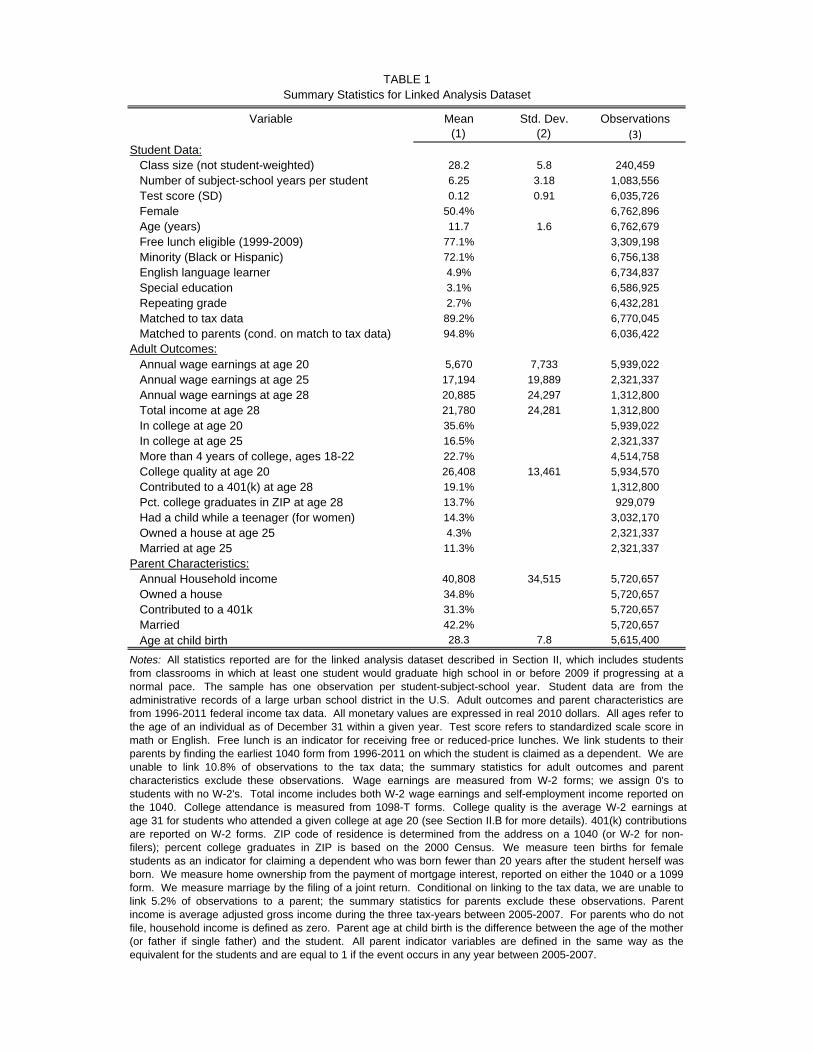
Variable Mean Std. Dev. Observations(1) (2) (3)

Student Data: Class size (not student-weighted) 28.2 5.8 240,459

Number of subject-school years per student 6.25 3.18 1,083,556

Test score (SD) 0.12 0.91 6,035,726

Female 50.4% 6,762,896

Age (years) 11.7 1.6 6,762,679

Free lunch eligible (1999-2009) 77.1% 3,309,198

Minority (Black or Hispanic) 72.1% 6,756,138

English language learner 4.9% 6,734,837

Special education 3.1% 6,586,925

Repeating grade 2.7% 6,432,281

Matched to tax data 89.2% 6,770,045

Matched to parents (cond. on match to tax data) 94.8% 6,036,422

Adult Outcomes: Annual wage earnings at age 20 5,670 7,733 5,939,022

Annual wage earnings at age 25 17,194 19,889 2,321,337

Annual wage earnings at age 28 20,885 24,297 1,312,800

Total income at age 28 21,780 24,281 1,312,800

In college at age 20 35.6% 5,939,022

In college at age 25 16.5% 2,321,337

More than 4 years of college, ages 18-22 22.7% 4,514,758

College quality at age 20 26,408 13,461 5,934,570

Contributed to a 401(k) at age 28 19.1% 1,312,800

Pct. college graduates in ZIP at age 28 13.7% 929,079

Had a child while a teenager (for women) 14.3% 3,032,170

Owned a house at age 25 4.3% 2,321,337

Married at age 25 11.3% 2,321,337

Parent Characteristics: Annual Household income 40,808 34,515 5,720,657

Owned a house 34.8% 5,720,657

Contributed to a 401k 31.3% 5,720,657

Married 42.2% 5,720,657

Age at child birth 28.3 7.8 5,615,400

TABLE 1Summary Statistics for Linked Analysis Dataset

Notes: All statistics reported are for the linked analysis dataset described in Section II, which includes students from classrooms in which at least one student would graduate high school in or before 2009 if progressing at a normal pace. The sample has one observation per student-subject-school year. Student data are from the administrative records of a large urban school district in the U.S. Adult outcomes and parent characteristics are from 1996-2011 federal income tax data. All monetary values are expressed in real 2010 dollars. All ages refer to the age of an individual as of December 31 within a given year. Test score refers to standardized scale score in math or English. Free lunch is an indicator for receiving free or reduced-price lunches. We link students to their parents by finding the earliest 1040 form from 1996-2011 on which the student is claimed as a dependent. We are unable to link 10.8% of observations to the tax data; the summary statistics for adult outcomes and parent characteristics exclude these observations. Wage earnings are measured from W-2 forms; we assign 0's to students with no W-2's. Total income includes both W-2 wage earnings and self-employment income reported on the 1040. College attendance is measured from 1098-T forms. College quality is the average W-2 earnings at age 31 for students who attended a given college at age 20 (see Section II.B for more details). 401(k) contributions are reported on W-2 forms. ZIP code of residence is determined from the address on a 1040 (or W-2 for non-filers); percent college graduates in ZIP is based on the 2000 Census. We measure teen births for female students as an indicator for claiming a dependent who was born fewer than 20 years after the student herself was born. We measure home ownership from the payment of mortgage interest, reported on either the 1040 or a 1099 form. We measure marriage by the filing of a joint return. Conditional on linking to the tax data, we are unable to link 5.2% of observations to a parent; the summary statistics for parents exclude these observations. Parent income is average adjusted gross income during the three tax-years between 2005-2007. For parents who do not file, household income is defined as zero. Parent age at child birth is the difference between the age of the mother (or father if single father) and the student. All parent indicator variables are defined in the same way as the equivalent for the students and are equal to 1 if the event occurs in any year between 2005-2007.

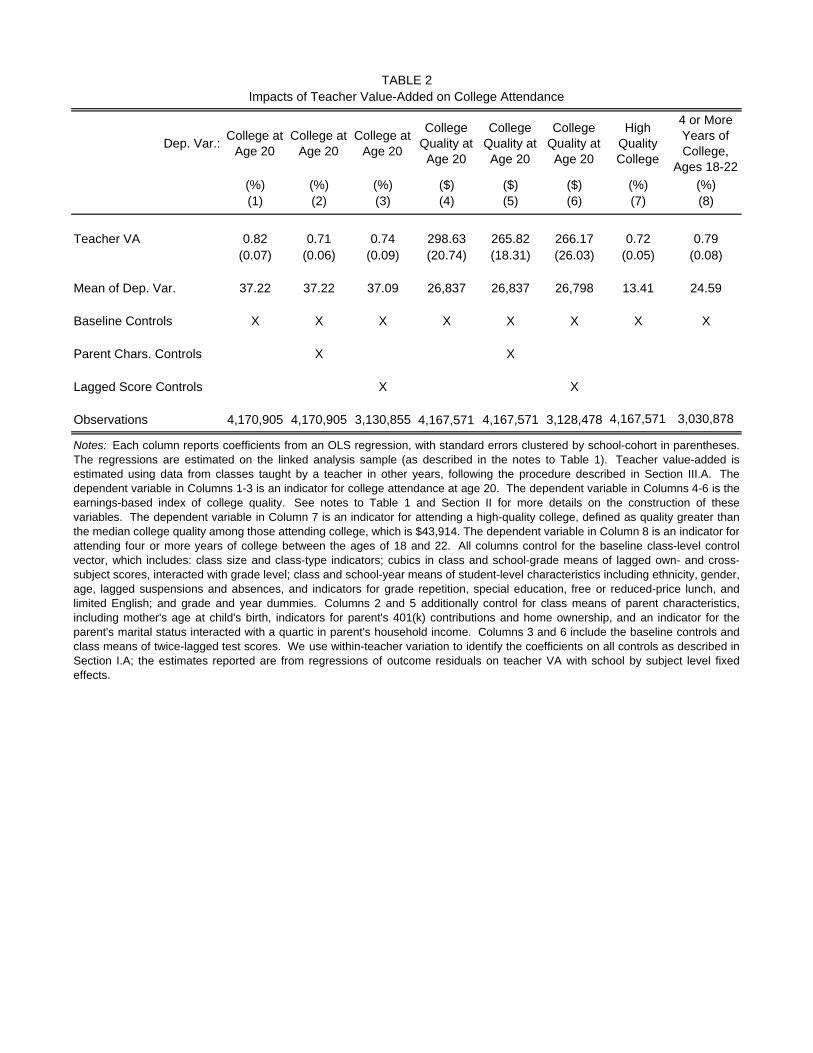
Dep. Var.:College at

Age 20College at

Age 20College at

Age 20

College Quality at Age 20



High Quality College

4 or More Years of College,

Ages 18-22

(%) (%) (%) ($) ($) ($) (%) (%)(1) (2) (3) (4) (5) (6) (7) (8)

Teacher VA 0.82 0.71 0.74 298.63 265.82 266.17 0.72 0.79(0.07) (0.06) (0.09) (20.74) (18.31) (26.03) (0.05) (0.08)

Mean of Dep. Var. 37.22 37.22 37.09 26,837 26,837 26,798 13.41 24.59

Baseline Controls X X X X X X X X

Parent Chars. Controls X X

Lagged Score Controls X X

Observations 4,170,905 4,170,905 3,130,855 4,167,571 4,167,571 3,128,478 4,167,571 3,030,878

Impacts of Teacher Value-Added on College AttendanceTABLE 2

Notes: Each column reports coefficients from an OLS regression, with standard errors clustered by school-cohort in parentheses.The regressions are estimated on the linked analysis sample (as described in the notes to Table 1). Teacher value-added isestimated using data from classes taught by a teacher in other years, following the procedure described in Section III.A. Thedependent variable in Columns 1-3 is an indicator for college attendance at age 20. The dependent variable in Columns 4-6 is theearnings-based index of college quality. See notes to Table 1 and Section II for more details on the construction of thesevariables. The dependent variable in Column 7 is an indicator for attending a high-quality college, defined as quality greater thanthe median college quality among those attending college, which is $43,914. The dependent variable in Column 8 is an indicator forattending four or more years of college between the ages of 18 and 22. All columns control for the baseline class-level controlvector, which includes: class size and class-type indicators; cubics in class and school-grade means of lagged own- and cross-subject scores, interacted with grade level; class and school-year means of student-level characteristics including ethnicity, gender,age, lagged suspensions and absences, and indicators for grade repetition, special education, free or reduced-price lunch, andlimited English; and grade and year dummies. Columns 2 and 5 additionally control for class means of parent characteristics,including mother's age at child's birth, indicators for parent's 401(k) contributions and home ownership, and an indicator for theparent's marital status interacted with a quartic in parent's household income. Columns 3 and 6 include the baseline controls andclass means of twice-lagged test scores. We use within-teacher variation to identify the coefficients on all controls as described inSection I.A; the estimates reported are from regressions of outcome residuals on teacher VA with school by subject level fixedeffects.

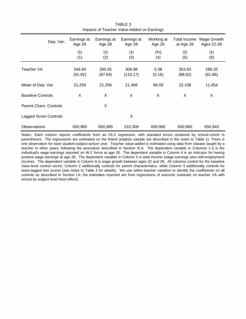
Dep. Var.:Earnings at

Age 28Earnings at

Age 28Earnings at

Age 28Working at

Age 28Total Income

at Age 28Wage Growth Ages 22-28

($) ($) ($) (%) ($) ($)

(1) (2) (3) (4) (5) (6)

Teacher VA 349.84 285.55 308.98 0.38 353.83 286.20(91.92) (87.64) (110.17) (0.16) (88.62) (81.86)

Mean of Dep. Var. 21,256 21,256 21,468 68.09 22,108 11,454

Baseline Controls X X X X X X

Parent Chars. Controls X

Lagged Score Controls X

Observations 650,965 650,965 510,309 650,965 650,965 650,943

Notes: Each column reports coefficients from an OLS regression, with standard errors clustered by school-cohort inparentheses. The regressions are estimated on the linked analysis sample (as described in the notes to Table 1). There isone observation for each student-subject-school year. Teacher value-added is estimated using data from classes taught by ateacher in other years, following the procedure described in Section III.A. The dependent variable in Columns 1-3 is theindividual's wage earnings reported on W-2 forms at age 28. The dependent variable in Column 4 is an indicator for havingpositive wage earnings at age 28. The dependent variable in Column 5 is total income (wage earnings plus self-employmentincome). The dependent variable in Column 6 is wage growth between ages 22 and 28. All columns control for the baselineclass-level control vector; Column 2 additionally controls for parent characteristics, while Column 3 additionally controls fortwice-lagged test scores (see notes to Table 2 for details). We use within-teacher variation to identify the coefficients on allcontrols as described in Section I.A; the estimates reported are from regressions of outcome residuals on teacher VA withschool by subject level fixed effects.

Impacts of Teacher Value-Added on EarningsTABLE 3

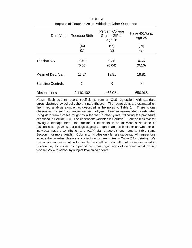
Dep. Var.: Teenage BirthPercent College Grad in ZIP at

Age 28

Have 401(k) at Age 28

(%) (%) (%)(1) (2) (3)

Teacher VA -0.61 0.25 0.55(0.06) (0.04) (0.16)

Mean of Dep. Var. 13.24 13.81 19.81

Baseline Controls X X X

Observations 2,110,402 468,021 650,965

TABLE 4Impacts of Teacher Value-Added on Other Outcomes

Notes: Each column reports coefficients from an OLS regression, with standarderrors clustered by school-cohort in parentheses. The regressions are estimated onthe linked analysis sample (as described in the notes to Table 1). There is oneobservation for each student-subject-school year. Teacher value-added is estimatedusing data from classes taught by a teacher in other years, following the proceduredescribed in Section III.A. The dependent variables in Column 1-3 are an indicator forhaving a teenage birth, the fraction of residents in an individual’s zip code ofresidence at age 28 with a college degree or higher, and an indicator for whether anindividual made a contribution to a 401(k) plan at age 28 (see notes to Table 1 andSection II for more details). Column 1 includes only female students. All regressionsinclude the baseline class-level control vector (see notes to Table 2 for details). Weuse within-teacher variation to identify the coefficients on all controls as described inSection I.A; the estimates reported are from regressions of outcome residuals onteacher VA with school by subject level fixed effects.

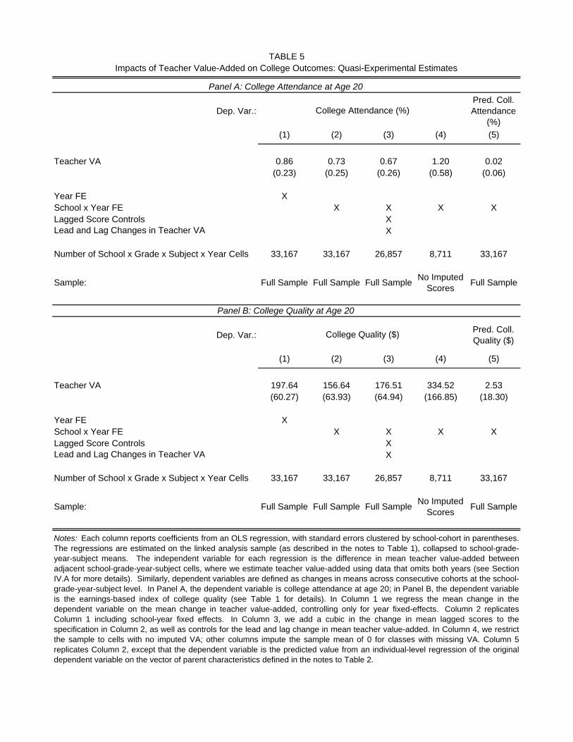
Dep. Var.:Pred. Coll. Attendance

(%)

(1) (2) (3) (4) (5)

Teacher VA 0.86 0.73 0.67 1.20 0.02(0.23) (0.25) (0.26) (0.58) (0.06)

Year FE XSchool x Year FE X X X XLagged Score Controls XLead and Lag Changes in Teacher VA X

Number of School x Grade x Subject x Year Cells 33,167 33,167 26,857 8,711 33,167

Sample: Full Sample Full Sample Full SampleNo Imputed

ScoresFull Sample

Dep. Var.:Pred. Coll.Quality ($)

(1) (2) (3) (4) (5)

Teacher VA 197.64 156.64 176.51 334.52 2.53(60.27) (63.93) (64.94) (166.85) (18.30)

Year FE XSchool x Year FE X X X XLagged Score Controls XLead and Lag Changes in Teacher VA X

Number of School x Grade x Subject x Year Cells 33,167 33,167 26,857 8,711 33,167

Sample: Full Sample Full Sample Full SampleNo Imputed

ScoresFull Sample

Panel A: College Attendance at Age 20

TABLE 5

Panel B: College Quality at Age 20

Notes: Each column reports coefficients from an OLS regression, with standard errors clustered by school-cohort in parentheses.The regressions are estimated on the linked analysis sample (as described in the notes to Table 1), collapsed to school-grade-year-subject means. The independent variable for each regression is the difference in mean teacher value-added betweenadjacent school-grade-year-subject cells, where we estimate teacher value-added using data that omits both years (see SectionIV.A for more details). Similarly, dependent variables are defined as changes in means across consecutive cohorts at the school-grade-year-subject level. In Panel A, the dependent variable is college attendance at age 20; in Panel B, the dependent variableis the earnings-based index of college quality (see Table 1 for details). In Column 1 we regress the mean change in thedependent variable on the mean change in teacher value-added, controlling only for year fixed-effects. Column 2 replicatesColumn 1 including school-year fixed effects. In Column 3, we add a cubic in the change in mean lagged scores to thespecification in Column 2, as well as controls for the lead and lag change in mean teacher value-added. In Column 4, we restrictthe sample to cells with no imputed VA; other columns impute the sample mean of 0 for classes with missing VA. Column 5replicates Column 2, except that the dependent variable is the predicted value from an individual-level regression of the originaldependent variable on the vector of parent characteristics defined in the notes to Table 2.

Impacts of Teacher Value-Added on College Outcomes: Quasi-Experimental Estimates

College Attendance (%)

College Quality ($)

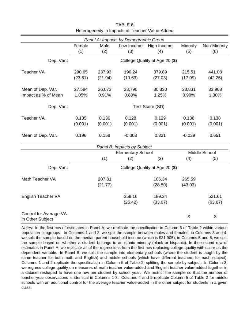
Female Male Low Income High Income Minority Non-Minority(1) (2) (3) (4) (5) (6)

Dep. Var.:

Teacher VA 290.65 237.93 190.24 379.89 215.51 441.08(23.61) (21.94) (19.63) (27.03) (17.09) (42.26)

Mean of Dep. Var. 27,584 26,073 23,790 30,330 23,831 33,968Impact as % of Mean 1.05% 0.91% 0.80% 1.25% 0.90% 1.30%

Dep. Var.:

Teacher VA 0.135 0.136 0.128 0.129 0.136 0.138(0.001) (0.001) (0.001) (0.001) (0.001) (0.001)

Mean of Dep. Var. 0.196 0.158 -0.003 0.331 -0.039 0.651

(1) (2) (3) (4) (5)

Dep. Var.:

Math Teacher VA 207.81 106.34 265.59(21.77) (28.50) (43.03)

English Teacher VA 258.16 189.24 521.61(25.42) (33.07) (63.67)

Control for Average VA in Other Subject

X X

Notes: In the first row of estimates in Panel A, we replicate the specification in Column 5 of Table 2 within variouspopulation subgroups. In Columns 1 and 2, we split the sample between males and females; in Columns 3 and 4,we split the sample based on the median parent household income (which is $31,905); in Columns 5 and 6, we splitthe sample based on whether a student belongs to an ethnic minority (black or hispanic). In the second row ofestimates in Panel A, we replicate all of the regressions from the first row replacing college quality with score as thedependent variable. In Panel B, we split the sample into elementary schools (where the student is taught by thesame teacher for both math and English) and middle schools (which have different teachers for each subject).Columns 1 and 2 replicate the specification in Column 5 of Table 2, splitting the sample by subject. In Column 3,we regress college quality on measures of math teacher value-added and English teacher value-added together ina dataset reshaped to have one row per student by school year. We restrict the sample so that the number ofteacher-year observations is identical in Columns 1-3. Columns 4 and 5 replicate Column 5 of Table 2 for middleschools with an additional control for the average teacher value-added in the other subject for students in a givenclass.

College Quality at Age 20 ($)

Middle School

TABLE 6Heterogeneity in Impacts of Teacher Value-Added

Panel A: Impacts by Demographic Group

Panel B: Impacts by SubjectElementary School

College Quality at Age 20 ($)

Test Score (SD)

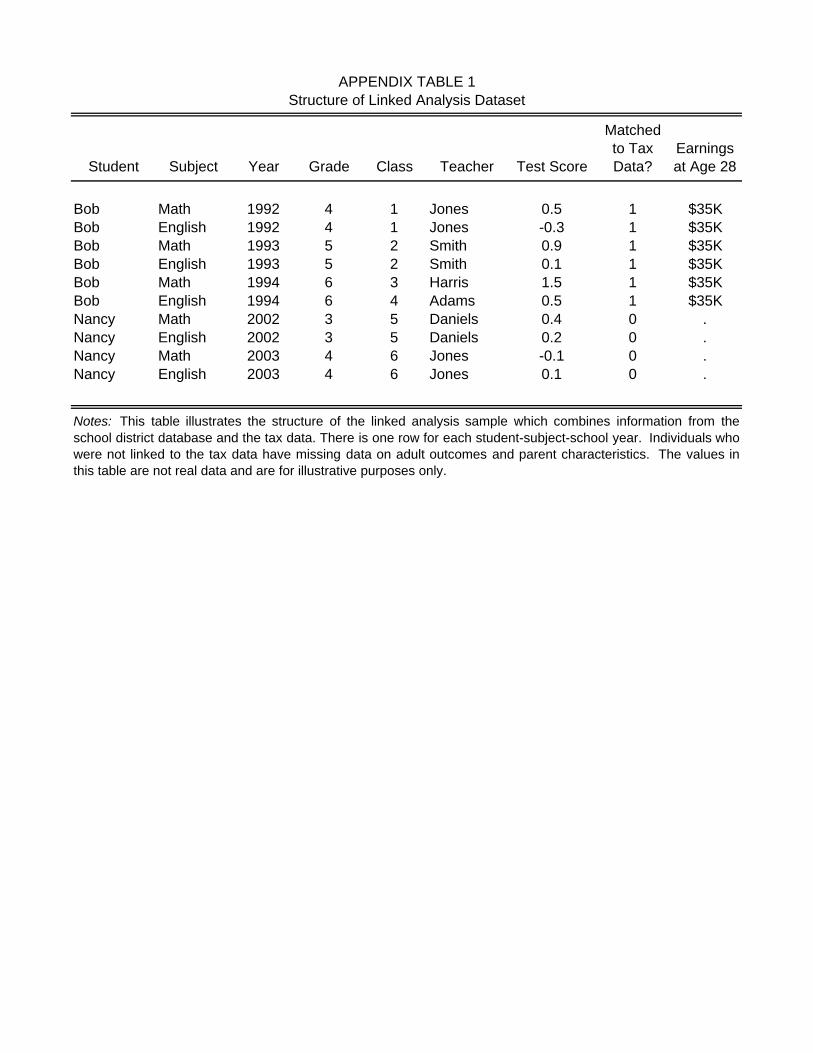
Student Subject Year Grade Class Teacher Test Score

Matchedto TaxData?

Earnings at Age 28

Bob Math 1992 4 1 Jones 0.5 1 $35KBob English 1992 4 1 Jones -0.3 1 $35KBob Math 1993 5 2 Smith 0.9 1 $35KBob English 1993 5 2 Smith 0.1 1 $35KBob Math 1994 6 3 Harris 1.5 1 $35KBob English 1994 6 4 Adams 0.5 1 $35KNancy Math 2002 3 5 Daniels 0.4 0 .Nancy English 2002 3 5 Daniels 0.2 0 .Nancy Math 2003 4 6 Jones -0.1 0 .Nancy English 2003 4 6 Jones 0.1 0 .

APPENDIX TABLE 1Structure of Linked Analysis Dataset

Notes: This table illustrates the structure of the linked analysis sample which combines information from theschool district database and the tax data. There is one row for each student-subject-school year. Individuals whowere not linked to the tax data have missing data on adult outcomes and parent characteristics. The values inthis table are not real data and are for illustrative purposes only.

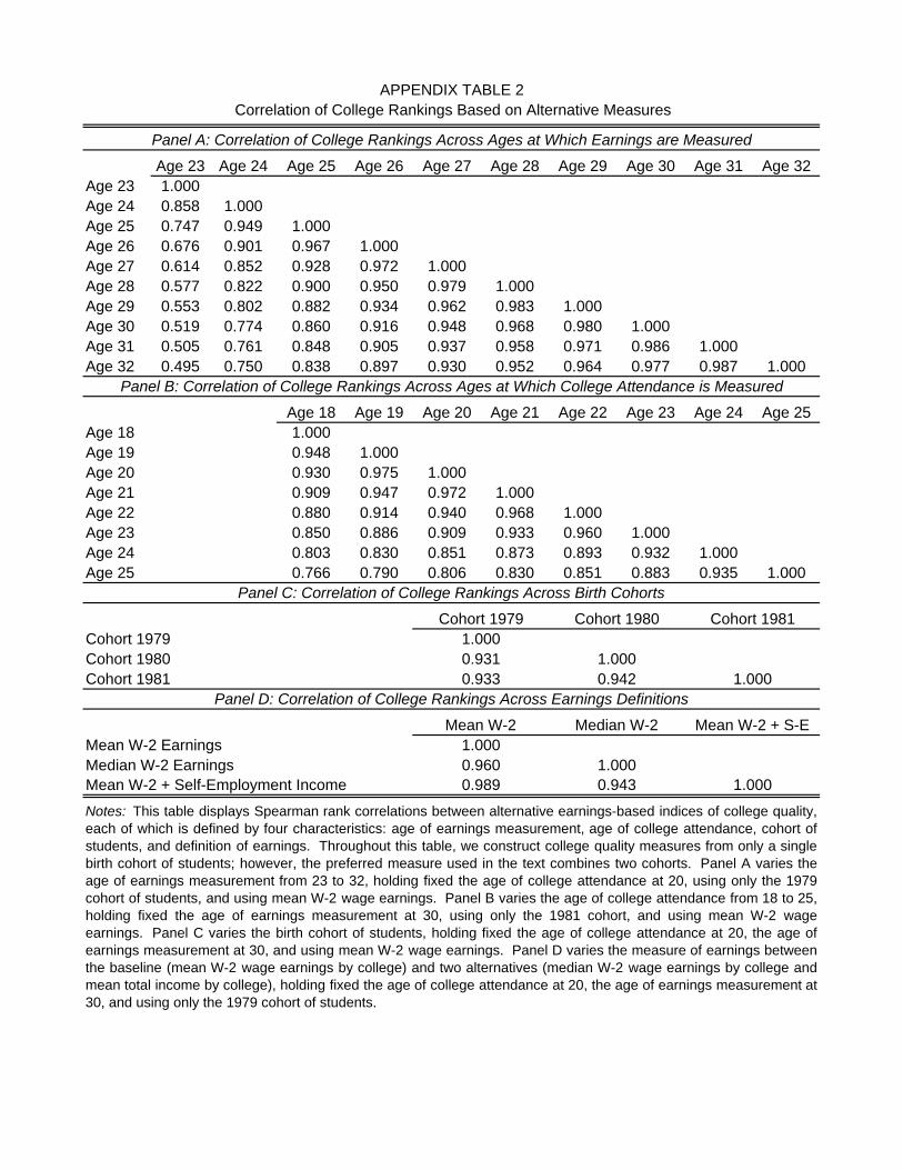
Age 23 Age 24 Age 25 Age 26 Age 27 Age 28 Age 29 Age 30 Age 31 Age 32Age 23 1.000Age 24 0.858 1.000Age 25 0.747 0.949 1.000Age 26 0.676 0.901 0.967 1.000Age 27 0.614 0.852 0.928 0.972 1.000Age 28 0.577 0.822 0.900 0.950 0.979 1.000Age 29 0.553 0.802 0.882 0.934 0.962 0.983 1.000Age 30 0.519 0.774 0.860 0.916 0.948 0.968 0.980 1.000Age 31 0.505 0.761 0.848 0.905 0.937 0.958 0.971 0.986 1.000Age 32 0.495 0.750 0.838 0.897 0.930 0.952 0.964 0.977 0.987 1.000

Age 18 Age 19 Age 20 Age 21 Age 22 Age 23 Age 24 Age 25Age 18 1.000Age 19 0.948 1.000Age 20 0.930 0.975 1.000Age 21 0.909 0.947 0.972 1.000Age 22 0.880 0.914 0.940 0.968 1.000Age 23 0.850 0.886 0.909 0.933 0.960 1.000Age 24 0.803 0.830 0.851 0.873 0.893 0.932 1.000Age 25 0.766 0.790 0.806 0.830 0.851 0.883 0.935 1.000

Panel D: Correlation of College Rankings Across Earnings Definitions

Cohort 1980

1.000

Cohort 19791.0000.9310.933

Cohort 1980Cohort 1981 0.942

Cohort 1981

1.000

Cohort 1979

APPENDIX TABLE 2

Panel B: Correlation of College Rankings Across Ages at Which College Attendance is Measured

Correlation of College Rankings Based on Alternative Measures

Panel C: Correlation of College Rankings Across Birth Cohorts

Panel A: Correlation of College Rankings Across Ages at Which Earnings are Measured

Mean W-2 + Self-Employment IncomeMedian W-2 Earnings

Notes: This table displays Spearman rank correlations between alternative earnings-based indices of college quality,each of which is defined by four characteristics: age of earnings measurement, age of college attendance, cohort ofstudents, and definition of earnings. Throughout this table, we construct college quality measures from only a singlebirth cohort of students; however, the preferred measure used in the text combines two cohorts. Panel A varies theage of earnings measurement from 23 to 32, holding fixed the age of college attendance at 20, using only the 1979cohort of students, and using mean W-2 wage earnings. Panel B varies the age of college attendance from 18 to 25,holding fixed the age of earnings measurement at 30, using only the 1981 cohort, and using mean W-2 wageearnings. Panel C varies the birth cohort of students, holding fixed the age of college attendance at 20, the age ofearnings measurement at 30, and using mean W-2 wage earnings. Panel D varies the measure of earnings betweenthe baseline (mean W-2 wage earnings by college) and two alternatives (median W-2 wage earnings by college andmean total income by college), holding fixed the age of college attendance at 20, the age of earnings measurement at30, and using only the 1979 cohort of students.

1.000

Mean W-2 + S-E

0.989

Median W-2

1.0000.943

Mean W-2

0.960Mean W-2 Earnings 1.000

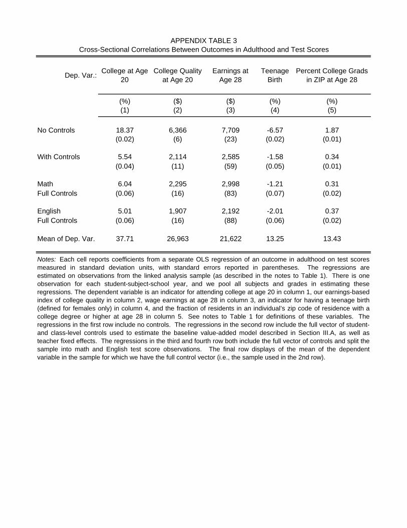
Dep. Var.:College at Age

20College Quality

at Age 20Earnings at

Age 28Teenage

BirthPercent College Grads

in ZIP at Age 28

(%) ($) ($) (%) (%)(1) (2) (3) (4) (5)

No Controls 18.37 6,366 7,709 -6.57 1.87(0.02) (6) (23) (0.02) (0.01)

With Controls 5.54 2,114 2,585 -1.58 0.34(0.04) (11) (59) (0.05) (0.01)

Math 6.04 2,295 2,998 -1.21 0.31Full Controls (0.06) (16) (83) (0.07) (0.02)

English 5.01 1,907 2,192 -2.01 0.37Full Controls (0.06) (16) (88) (0.06) (0.02)

Mean of Dep. Var. 37.71 26,963 21,622 13.25 13.43

APPENDIX TABLE 3Cross-Sectional Correlations Between Outcomes in Adulthood and Test Scores

Notes: Each cell reports coefficients from a separate OLS regression of an outcome in adulthood on test scoresmeasured in standard deviation units, with standard errors reported in parentheses. The regressions areestimated on observations from the linked analysis sample (as described in the notes to Table 1). There is oneobservation for each student-subject-school year, and we pool all subjects and grades in estimating theseregressions. The dependent variable is an indicator for attending college at age 20 in column 1, our earnings-basedindex of college quality in column 2, wage earnings at age 28 in column 3, an indicator for having a teenage birth(defined for females only) in column 4, and the fraction of residents in an individual’s zip code of residence with acollege degree or higher at age 28 in column 5. See notes to Table 1 for definitions of these variables. Theregressions in the first row include no controls. The regressions in the second row include the full vector of student-and class-level controls used to estimate the baseline value-added model described in Section III.A, as well asteacher fixed effects. The regressions in the third and fourth row both include the full vector of controls and split thesample into math and English test score observations. The final row displays of the mean of the dependentvariable in the sample for which we have the full control vector (i.e., the sample used in the 2nd row).

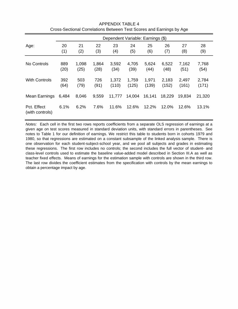
Age: 20 21 22 23 24 25 26 27 28(1) (2) (3) (4) (5) (6) (7) (8) (9)

No Controls 889 1,098 1,864 3,592 4,705 5,624 6,522 7,162 7,768(20) (25) (28) (34) (39) (44) (48) (51) (54)

With Controls 392 503 726 1,372 1,759 1,971 2,183 2,497 2,784(64) (79) (91) (110) (125) (139) (152) (161) (171)

Mean Earnings 6,484 8,046 9,559 11,777 14,004 16,141 18,229 19,834 21,320

Pct. Effect 6.1% 6.2% 7.6% 11.6% 12.6% 12.2% 12.0% 12.6% 13.1%(with controls)

APPENDIX TABLE 4Cross-Sectional Correlations Between Test Scores and Earnings by Age

Dependent Variable: Earnings ($)

Notes: Each cell in the first two rows reports coefficients from a separate OLS regression of earnings at agiven age on test scores measured in standard deviation units, with standard errors in parentheses. Seenotes to Table 1 for our definition of earnings. We restrict this table to students born in cohorts 1979 and1980, so that regressions are estimated on a constant subsample of the linked analysis sample. There isone observation for each student-subject-school year, and we pool all subjects and grades in estimatingthese regressions. The first row includes no controls; the second includes the full vector of student- andclass-level controls used to estimate the baseline value-added model described in Section III.A as well asteacher fixed effects. Means of earnings for the estimation sample with controls are shown in the third row.The last row divides the coefficient estimates from the specification with controls by the mean earnings toobtain a percentage impact by age.

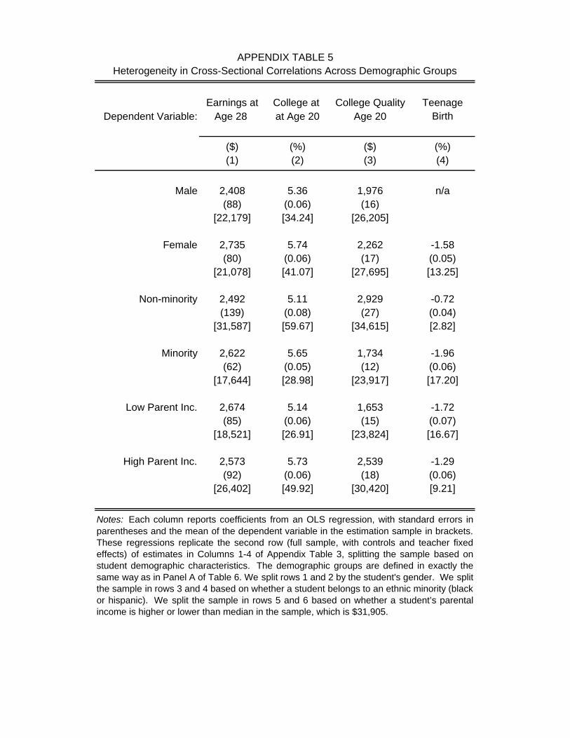
Earnings at College at College Quality TeenageDependent Variable: Age 28 at Age 20 Age 20 Birth

($) (%) ($) (%)(1) (2) (3) (4)

Male 2,408 5.36 1,976 n/a(88) (0.06) (16)

[22,179] [34.24] [26,205]

Female 2,735 5.74 2,262 -1.58(80) (0.06) (17) (0.05)

[21,078] [41.07] [27,695] [13.25]

Non-minority 2,492 5.11 2,929 -0.72(139) (0.08) (27) (0.04)

[31,587] [59.67] [34,615] [2.82]

Minority 2,622 5.65 1,734 -1.96(62) (0.05) (12) (0.06)

[17,644] [28.98] [23,917] [17.20]

Low Parent Inc. 2,674 5.14 1,653 -1.72(85) (0.06) (15) (0.07)

[18,521] [26.91] [23,824] [16.67]

High Parent Inc. 2,573 5.73 2,539 -1.29(92) (0.06) (18) (0.06)

[26,402] [49.92] [30,420] [9.21]

APPENDIX TABLE 5Heterogeneity in Cross-Sectional Correlations Across Demographic Groups

Notes: Each column reports coefficients from an OLS regression, with standard errors inparentheses and the mean of the dependent variable in the estimation sample in brackets.These regressions replicate the second row (full sample, with controls and teacher fixedeffects) of estimates in Columns 1-4 of Appendix Table 3, splitting the sample based onstudent demographic characteristics. The demographic groups are defined in exactly thesame way as in Panel A of Table 6. We split rows 1 and 2 by the student's gender. We splitthe sample in rows 3 and 4 based on whether a student belongs to an ethnic minority (blackor hispanic). We split the sample in rows 5 and 6 based on whether a student’s parentalincome is higher or lower than median in the sample, which is $31,905.

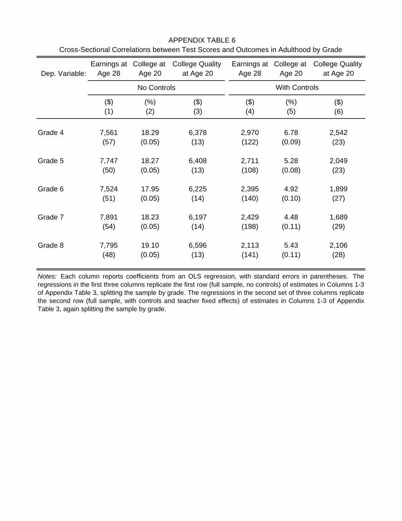
Earnings at College at College Quality Earnings at College at College Quality Dep. Variable: Age 28 Age 20 at Age 20 Age 28 Age 20 at Age 20

($) (%) ($) ($) (%) ($)(1) (2) (3) (4) (5) (6)

Grade 4 7,561 18.29 6,378 2,970 6.78 2,542(57) (0.05) (13) (122) (0.09) (23)

Grade 5 7,747 18.27 6,408 2,711 5.28 2,049(50) (0.05) (13) (108) (0.08) (23)

Grade 6 7,524 17.95 6,225 2,395 4.92 1,899(51) (0.05) (14) (140) (0.10) (27)

Grade 7 7,891 18.23 6,197 2,429 4.48 1,689(54) (0.05) (14) (198) (0.11) (29)

Grade 8 7,795 19.10 6,596 2,113 5.43 2,106(48) (0.05) (13) (141) (0.11) (28)

APPENDIX TABLE 6Cross-Sectional Correlations between Test Scores and Outcomes in Adulthood by Grade

No Controls With Controls

Notes: Each column reports coefficients from an OLS regression, with standard errors in parentheses. Theregressions in the first three columns replicate the first row (full sample, no controls) of estimates in Columns 1-3of Appendix Table 3, splitting the sample by grade. The regressions in the second set of three columns replicatethe second row (full sample, with controls and teacher fixed effects) of estimates in Columns 1-3 of AppendixTable 3, again splitting the sample by grade.

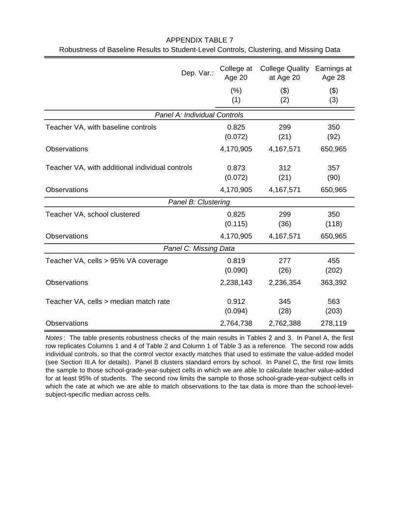
Dep. Var.:College at

Age 20College Quality

at Age 20Earnings at

Age 28

(%) ($) ($)(1) (2) (3)

Teacher VA, with baseline controls 0.825 299 350(0.072) (21) (92)

Observations 4,170,905 4,167,571 650,965

Teacher VA, with additional individual controls 0.873 312 357(0.072) (21) (90)

Observations 4,170,905 4,167,571 650,965

Teacher VA, school clustered 0.825 299 350(0.115) (36) (118)

Observations 4,170,905 4,167,571 650,965

Teacher VA, cells > 95% VA coverage 0.819 277 455(0.090) (26) (202)

Observations 2,238,143 2,236,354 363,392

Teacher VA, cells > median match rate 0.912 345 563(0.094) (28) (203)

Observations 2,764,738 2,762,388 278,119

APPENDIX TABLE 7Robustness of Baseline Results to Student-Level Controls, Clustering, and Missing Data

Notes : The table presents robustness checks of the main results in Tables 2 and 3. In Panel A, the firstrow replicates Columns 1 and 4 of Table 2 and Column 1 of Table 3 as a reference. The second row addsindividual controls, so that the control vector exactly matches that used to estimate the value-added model(see Section III.A for details). Panel B clusters standard errors by school. In Panel C, the first row limitsthe sample to those school-grade-year-subject cells in which we are able to calculate teacher value-addedfor at least 95% of students. The second row limits the sample to those school-grade-year-subject cells inwhich the rate at which we are able to match observations to the tax data is more than the school-level-subject-specific median across cells.

Panel A: Individual Controls

Panel B: Clustering

Panel C: Missing Data

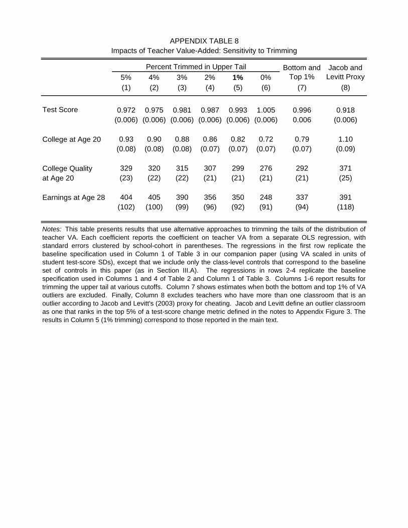
5% 4% 3% 2% 1% 0%(1) (2) (3) (4) (5) (6) (7) (8)

Test Score 0.972 0.975 0.981 0.987 0.993 1.005 0.996 0.918(0.006) (0.006) (0.006) (0.006) (0.006) (0.006) 0.006 (0.006)

College at Age 20 0.93 0.90 0.88 0.86 0.82 0.72 0.79 1.10(0.08) (0.08) (0.08) (0.07) (0.07) (0.07) (0.07) (0.09)

College Quality 329 320 315 307 299 276 292 371at Age 20 (23) (22) (22) (21) (21) (21) (21) (25)

Earnings at Age 28 404 405 390 356 350 248 337 391(102) (100) (99) (96) (92) (91) (94) (118)

Notes: This table presents results that use alternative approaches to trimming the tails of the distribution ofteacher VA. Each coefficient reports the coefficient on teacher VA from a separate OLS regression, withstandard errors clustered by school-cohort in parentheses. The regressions in the first row replicate thebaseline specification used in Column 1 of Table 3 in our companion paper (using VA scaled in units ofstudent test-score SDs), except that we include only the class-level controls that correspond to the baselineset of controls in this paper (as in Section III.A). The regressions in rows 2-4 replicate the baselinespecification used in Columns 1 and 4 of Table 2 and Column 1 of Table 3. Columns 1-6 report results fortrimming the upper tail at various cutoffs. Column 7 shows estimates when both the bottom and top 1% of VAoutliers are excluded. Finally, Column 8 excludes teachers who have more than one classroom that is anoutlier according to Jacob and Levitt's (2003) proxy for cheating. Jacob and Levitt define an outlier classroomas one that ranks in the top 5% of a test-score change metric defined in the notes to Appendix Figure 3. Theresults in Column 5 (1% trimming) correspond to those reported in the main text.

APPENDIX TABLE 8Impacts of Teacher Value-Added: Sensitivity to Trimming

Percent Trimmed in Upper Tail Bottom andTop 1%

Jacob andLevitt Proxy

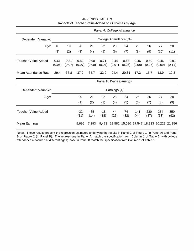
Dependent Variable:

Age: 18 19 20 21 22 23 24 25 26 27 28

(1) (2) (3) (4) (5) (6) (7) (8) (9) (10) (11)

Teacher Value-Added 0.61 0.81 0.82 0.98 0.71 0.44 0.58 0.46 0.50 0.46 -0.01(0.06) (0.07) (0.07) (0.08) (0.07) (0.07) (0.07) (0.08) (0.07) (0.09) (0.11)

Mean Attendance Rate 29.4 36.8 37.2 35.7 32.2 24.4 20.31 17.3 15.7 13.9 12.3

Dependent Variable:

Age: 20 21 22 23 24 25 26 27 28

(1) (2) (3) (4) (5) (6) (7) (8) (9)

Teacher Value-Added -32 -35 -18 44 74 141 230 254 350(11) (14) (18) (25) (32) (44) (47) (63) (92)

Mean Earnings 5,696 7,293 9,473 12,582 15,080 17,547 18,833 20,229 21,256

Panel B: Wage Earnings

Notes: These results present the regression estimates underlying the results in Panel C of Figure 1 (in Panel A) and PanelB of Figure 2 (in Panel B). The regressions in Panel A match the specification from Column 1 of Table 2, with collegeattendance measured at different ages; those in Panel B match the specification from Column 1 of Table 3.

Impacts of Teacher Value-Added on Outcomes by AgeAPPENDIX TABLE 9

College Attendance (%)

Panel A: College Attendance

Earnings ($)

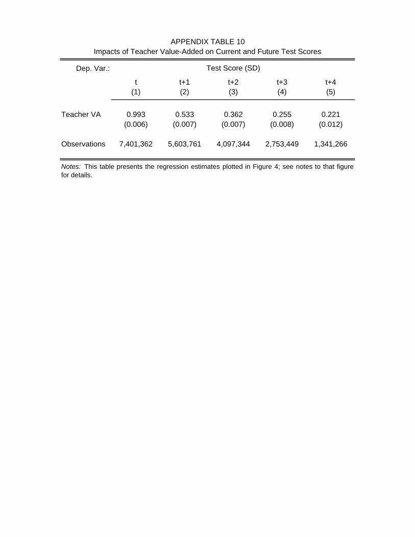
Dep. Var.:

t t+1 t+2 t+3 t+4(1) (2) (3) (4) (5)

Teacher VA 0.993 0.533 0.362 0.255 0.221(0.006) (0.007) (0.007) (0.008) (0.012)

Observations 7,401,362 5,603,761 4,097,344 2,753,449 1,341,266

APPENDIX TABLE 10Impacts of Teacher Value-Added on Current and Future Test Scores

Test Score (SD)

Notes: This table presents the regression estimates plotted in Figure 4; see notes to that figurefor details.

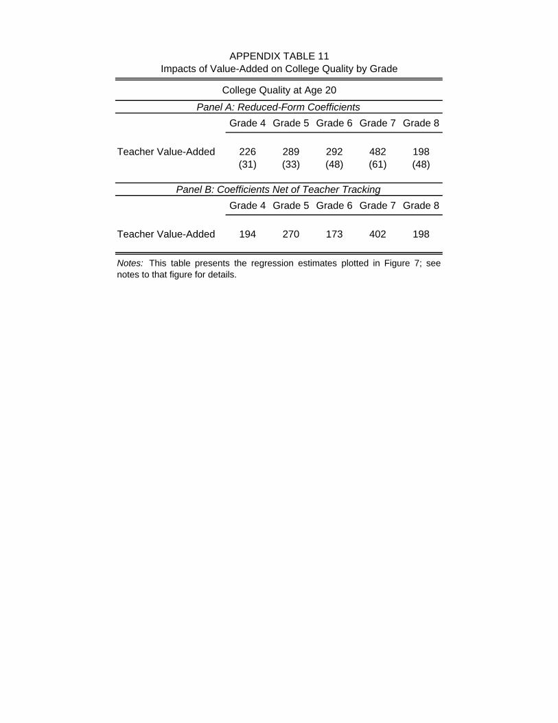
Grade 4 Grade 5 Grade 6 Grade 7 Grade 8

Teacher Value-Added 226 289 292 482 198(31) (33) (48) (61) (48)

Grade 4 Grade 5 Grade 6 Grade 7 Grade 8

Teacher Value-Added 194 270 173 402 198

Notes: This table presents the regression estimates plotted in Figure 7; seenotes to that figure for details.

APPENDIX TABLE 11Impacts of Value-Added on College Quality by Grade


Panel A: Reduced-Form Coefficients

Panel B: Coefficients Net of Teacher Tracking

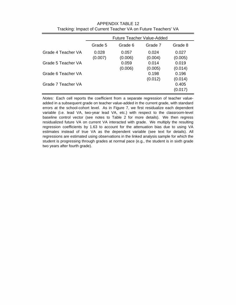
Grade 5 Grade 6 Grade 7 Grade 8

Grade 4 Teacher VA 0.028 0.057 0.024 0.027(0.007) (0.006) (0.004) (0.005)

Grade 5 Teacher VA 0.059 0.014 0.019(0.006) (0.005) (0.014)

Grade 6 Teacher VA 0.198 0.196(0.012) (0.014)

Grade 7 Teacher VA 0.405(0.017)

APPENDIX TABLE 12Tracking: Impact of Current Teacher VA on Future Teachers' VA

Future Teacher Value-Added

Notes: Each cell reports the coefficient from a separate regression of teacher value-added in a subsequent grade on teacher value-added in the current grade, with standarderrors at the school-cohort level. As in Figure 7, we first residualize each dependentvariable (i.e. lead VA, two-year lead VA, etc.) with respect to the classroom-levelbaseline control vector (see notes to Table 2 for more details). We then regressresidualized future VA on current VA interacted with grade. We multiply the resultingregression coefficients by 1.63 to account for the attenuation bias due to using VAestimates instead of true VA as the dependent variable (see text for details). Allregressions are estimated using observations in the linked analysis sample for which thestudent is progressing through grades at normal pace (e.g., the student is in sixth gradetwo years after fourth grade).

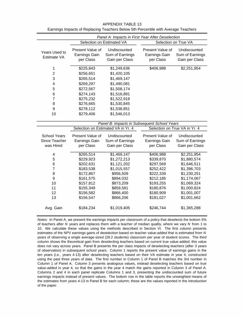
Years Used to Estimate VA

Present Value of Earnings Gain

per Class

Undiscounted Sum of Earnings Gain per Class


per Class


1 $225,843 $1,249,636 $406,988 $2,251,9542 $256,651 $1,420,1053 $265,514 $1,469,1474 $269,297 $1,490,0815 $272,567 $1,508,1746 $274,143 $1,516,8917 $275,232 $1,522,9188 $276,665 $1,530,8459 $278,112 $1,538,851

10 $279,406 $1,546,013

School Years Since Teacher

was Hired


per Class



per Class


4 $265,514 $1,469,147 $406,988 $2,251,9545 $229,923 $1,272,213 $339,870 $1,880,5746 $202,631 $1,121,202 $297,569 $1,646,5117 $183,538 $1,015,557 $252,422 $1,396,7038 $172,867 $956,509 $222,339 $1,230,2519 $161,575 $894,032 $212,185 $1,174,067

10 $157,812 $873,209 $193,255 $1,069,32411 $155,349 $859,581 $180,876 $1,000,82412 $156,582 $866,400 $180,909 $1,001,00713 $156,547 $866,206 $181,027 $1,001,662

Avg. Gain $184,234 $1,019,405 $246,744 $1,365,288

Notes: In Panel A, we present the earnings impacts per classroom of a policy that deselects the bottom 5%of teachers after N years and replaces them with a teacher of median quality, where we vary N from 1 to10. We calculate these values using the methods described in Section VI. The first column presentsestimates of the NPV earnings gains of deselection based on teacher value-added that is estimated from N years of observing a single average-sized (28.2 students) classroom per year of student scores. The thirdcolumn shows the theoretical gain from deselecting teachers based on current true value-added; this valuedoes not vary across years. Panel B presents the per class impacts of deselecting teachers (after 3 yearsof observation) in subsequent school years. Column 1 reports the present value of earnings gains in theten years (i.e., years 4-13) after deselecting teachers based on their VA estimate in year 4, constructedusing the past three years of data. The first number in Column 1 of Panel B matches the 3rd number inColumn 1 of Panel A. Column 3 presents analogous values, instead deselecting teachers based on truevalue-added in year 4, so that the gains in the year 4 match the gains reported in Column 3 of Panel A.Columns 2 and 4 in each panel replicate Columns 1 and 3, presenting the undiscounted sum of futureearnings impacts instead of present values. The bottom row in the table reports the unweighted means ofthe estimates from years 4-13 in Panel B for each column; these are the values reported in the introductionof the paper.

Earnings Impacts of Replacing Teachers Below 5th Percentile with Average TeachersAPPENDIX TABLE 13

Panel B: Impacts in Subsequent School Years

Selection on Estimated VA Selection on True VAPanel A: Impacts in First Year After Deselection

Selection on Estimated VA in Yr. 4 Selection on True VA in Yr. 4

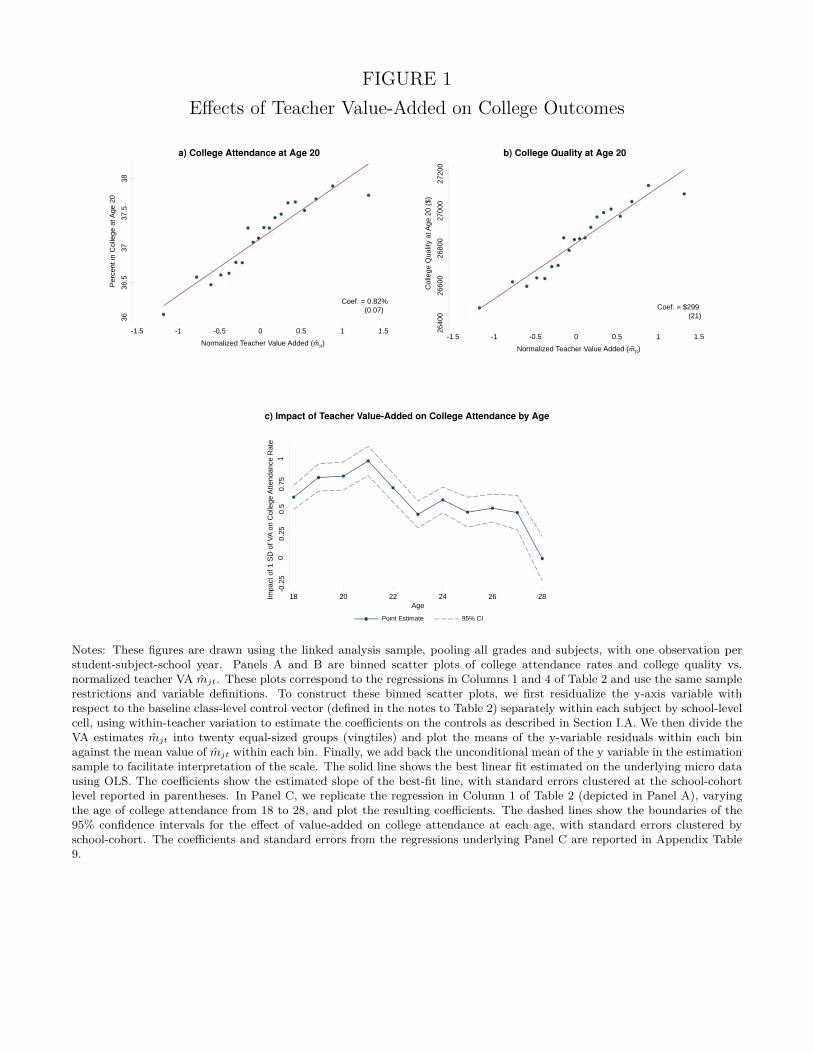
FIGURE 1Effects of Teacher Value-Added on College Outcomes

a) College Attendance at Age 20

3636

.537

37.5

38

Per

cent

in C

olle

ge a

t Age

20

-1.5 -1 -0.5 0 0.5 1 1.5

Normalized Teacher Value Added ( ��)

Coef. = 0.82%(0.07)

b) College Quality at Age 20

2640

026

600

2680

027

000

2720

0

Col

lege

Qua

lity

at A

ge 2

0 ($

)


Coef. = $299(21)

-1.5 -1 -0.5 0 0.5 1 1.5

c) Impact of Teacher Value-Added on College Attendance by Age

-0.2

50

0.25

0.5

0.75

1

18 20 22 24 26 28Impa

ct o

f 1 S

D o

f VA

on

Col

lege

Atte

ndan

ce R

ate

Age

Point Estimate 95% CI

Notes: These figures are drawn using the linked analysis sample, pooling all grades and subjects, with one observation perstudent-subject-school year. Panels A and B are binned scatter plots of college attendance rates and college quality vs.normalized teacher VA mjt. These plots correspond to the regressions in Columns 1 and 4 of Table 2 and use the same samplerestrictions and variable definitions. To construct these binned scatter plots, we first residualize the y-axis variable withrespect to the baseline class-level control vector (defined in the notes to Table 2) separately within each subject by school-levelcell, using within-teacher variation to estimate the coefficients on the controls as described in Section I.A. We then divide theVA estimates mjt into twenty equal-sized groups (vingtiles) and plot the means of the y-variable residuals within each binagainst the mean value of mjt within each bin. Finally, we add back the unconditional mean of the y variable in the estimationsample to facilitate interpretation of the scale. The solid line shows the best linear fit estimated on the underlying micro datausing OLS. The coefficients show the estimated slope of the best-fit line, with standard errors clustered at the school-cohortlevel reported in parentheses. In Panel C, we replicate the regression in Column 1 of Table 2 (depicted in Panel A), varyingthe age of college attendance from 18 to 28, and plot the resulting coefficients. The dashed lines show the boundaries of the95% confidence intervals for the effect of value-added on college attendance at each age, with standard errors clustered byschool-cohort. The coefficients and standard errors from the regressions underlying Panel C are reported in Appendix Table9.

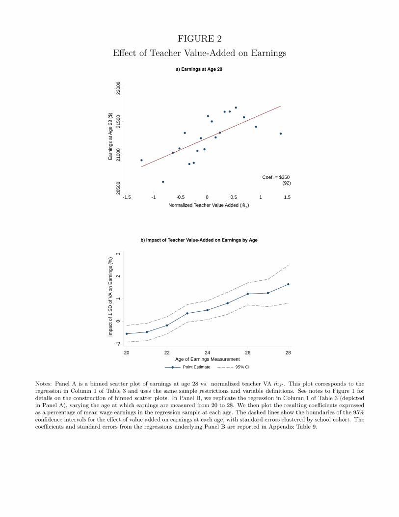
FIGURE 2Effect of Teacher Value-Added on Earnings

a) Earnings at Age 28

2050

021

000

2150

022

000

Ear

ning

s at

Age

28

($)

Coef. = $350(92)


-1.5 -1 -0.5 0 0.5 1 1.5

b) Impact of Teacher Value-Added on Earnings by Age

-10

12

3

Impa

ct o

f 1 S

D o

f VA

on

Ear

ning

s (%

)

20 22 24 26 28Age of Earnings Measurement


Notes: Panel A is a binned scatter plot of earnings at age 28 vs. normalized teacher VA mjt. This plot corresponds to theregression in Column 1 of Table 3 and uses the same sample restrictions and variable definitions. See notes to Figure 1 fordetails on the construction of binned scatter plots. In Panel B, we replicate the regression in Column 1 of Table 3 (depictedin Panel A), varying the age at which earnings are measured from 20 to 28. We then plot the resulting coefficients expressedas a percentage of mean wage earnings in the regression sample at each age. The dashed lines show the boundaries of the 95%confidence intervals for the effect of value-added on earnings at each age, with standard errors clustered by school-cohort. Thecoefficients and standard errors from the regressions underlying Panel B are reported in Appendix Table 9.

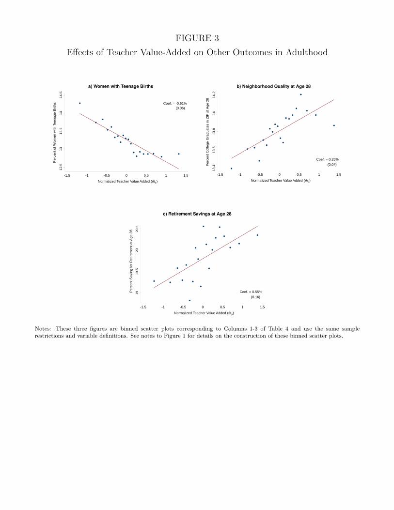
FIGURE 3Effects of Teacher Value-Added on Other Outcomes in Adulthood

a) Women with Teenage Births

12.5

1313

.514

14.5

Per

cent

of W

omen

with

Tee

nage

Birt

hs Coef. = -0.61%(0.06)


-1.5 -1 -0.5 0 0.5 1 1.5

b) Neighborhood Quality at Age 28

13.4

13.6

13.8

1414

.2

Per

cent

Col

lege

Gra

duat

es in

ZIP

at A

ge 2

8

Coef. = 0.25%

(0.04)


-1.5 -1 -0.5 0 0.5 1 1.5

c) Retirement Savings at Age 28

1919

.520

20.5

Per

cent

Sav

ing

for

Ret

irem

enta

t Age

28


Coef. = 0.55%

(0.16)

-1.5 -1 -0.5 0 0.5 1 1.5

Notes: These three figures are binned scatter plots corresponding to Columns 1-3 of Table 4 and use the same samplerestrictions and variable definitions. See notes to Figure 1 for details on the construction of these binned scatter plots.

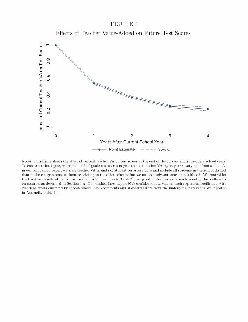
FIGURE 4Effects of Teacher Value-Added on Future Test Scores

00.

20.

40.

60.

81

Impa

ct o

f Cur

rent

Tea

cher

VA

on

Test

Sco

res

0 1 2 3 4Years After Current School Year


Notes: This figure shows the effect of current teacher VA on test scores at the end of the current and subsequent school years.To construct this figure, we regress end-of-grade test scores in year t+ s on teacher VA µjt in year t, varying s from 0 to 4. Asin our companion paper, we scale teacher VA in units of student test-score SD’s and include all students in the school districtdata in these regressions, without restricting to the older cohorts that we use to study outcomes in adulthood. We control forthe baseline class-level control vector (defined in the notes to Table 2), using within-teacher variation to identify the coefficientson controls as described in Section I.A. The dashed lines depict 95% confidence intervals on each regression coefficient, withstandard errors clustered by school-cohort. The coefficients and standard errors from the underlying regressions are reportedin Appendix Table 10.

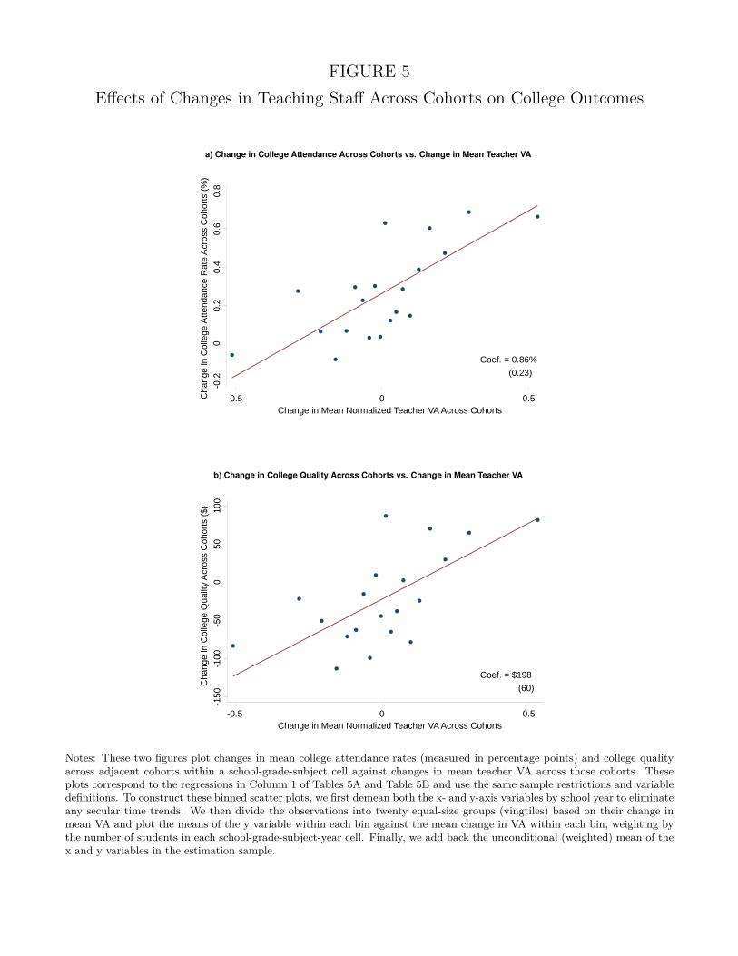
FIGURE 5Effects of Changes in Teaching Staff Across Cohorts on College Outcomes

a) Change in College Attendance Across Cohorts vs. Change in Mean Teacher VA

-0.2

00.

20.

40.

60.

8

-0.5 0 0.5Cha

nge

in C

olle

ge A

ttend

ance

Rat

e A

cros

s C

ohor

ts (

%)

Change in Mean Normalized Teacher VA Across Cohorts

Coef. = 0.86%

(0.23)

b) Change in College Quality Across Cohorts vs. Change in Mean Teacher VA

-150

-100

-50

050

100

Cha

nge

in C

olle

ge Q

ualit

y A

cros

s C

ohor

ts (

$)

Change in Mean Normalized Teacher VA Across Cohorts

Coef. = $198

(60)

-0.5 0 0.5

Notes: These two figures plot changes in mean college attendance rates (measured in percentage points) and college qualityacross adjacent cohorts within a school-grade-subject cell against changes in mean teacher VA across those cohorts. Theseplots correspond to the regressions in Column 1 of Tables 5A and Table 5B and use the same sample restrictions and variabledefinitions. To construct these binned scatter plots, we first demean both the x- and y-axis variables by school year to eliminateany secular time trends. We then divide the observations into twenty equal-size groups (vingtiles) based on their change inmean VA and plot the means of the y variable within each bin against the mean change in VA within each bin, weighting bythe number of students in each school-grade-subject-year cell. Finally, we add back the unconditional (weighted) mean of thex and y variables in the estimation sample.

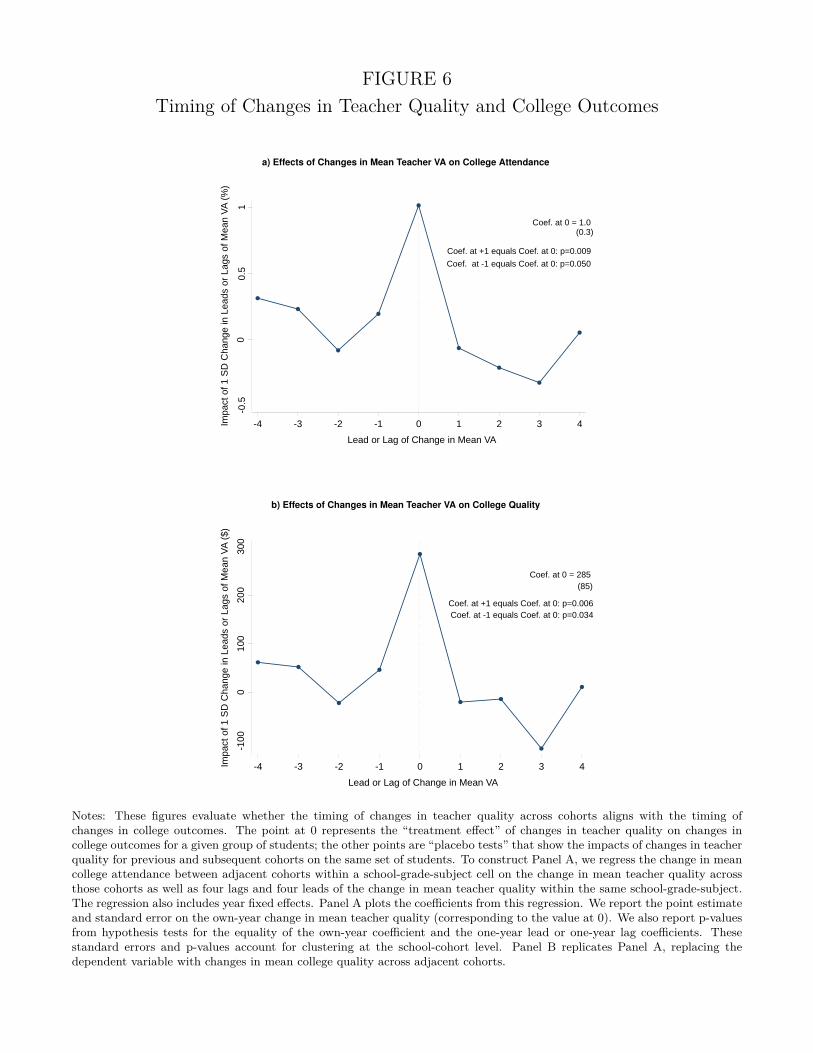
FIGURE 6Timing of Changes in Teacher Quality and College Outcomes

a) Effects of Changes in Mean Teacher VA on College Attendance

-0.5

00.

51

-4 -3 -2 -1 0 1 2 3 4

Coef. at 0 = 1.0(0.3)

Coef. at +1 equals Coef. at 0: p=0.009

Coef. at -1 equals Coef. at 0: p=0.050

Impa

ct o

f 1 S

D C

hang

e in

Lea

dsor

Lag

s of

Mea

n V

A (

%)

Lead or Lag of Change in Mean VA

b) Effects of Changes in Mean Teacher VA on College Quality

-100

010

020

030

0

-4 -3 -2 -1 0 1 2 3 4

Coef. at 0 = 285(85)

Coef. at +1 equals Coef. at 0: p=0.006Coef. at -1 equals Coef. at 0: p=0.034

Impa

ct o

f 1 S

D C

hang

e in

Lea

dsor

Lag

s of

Mea

n V

A (

$)

Lead or Lag of Change in Mean VA

Notes: These figures evaluate whether the timing of changes in teacher quality across cohorts aligns with the timing ofchanges in college outcomes. The point at 0 represents the “treatment effect” of changes in teacher quality on changes incollege outcomes for a given group of students; the other points are “placebo tests” that show the impacts of changes in teacherquality for previous and subsequent cohorts on the same set of students. To construct Panel A, we regress the change in meancollege attendance between adjacent cohorts within a school-grade-subject cell on the change in mean teacher quality acrossthose cohorts as well as four lags and four leads of the change in mean teacher quality within the same school-grade-subject.The regression also includes year fixed effects. Panel A plots the coefficients from this regression. We report the point estimateand standard error on the own-year change in mean teacher quality (corresponding to the value at 0). We also report p-valuesfrom hypothesis tests for the equality of the own-year coefficient and the one-year lead or one-year lag coefficients. Thesestandard errors and p-values account for clustering at the school-cohort level. Panel B replicates Panel A, replacing thedependent variable with changes in mean college quality across adjacent cohorts.

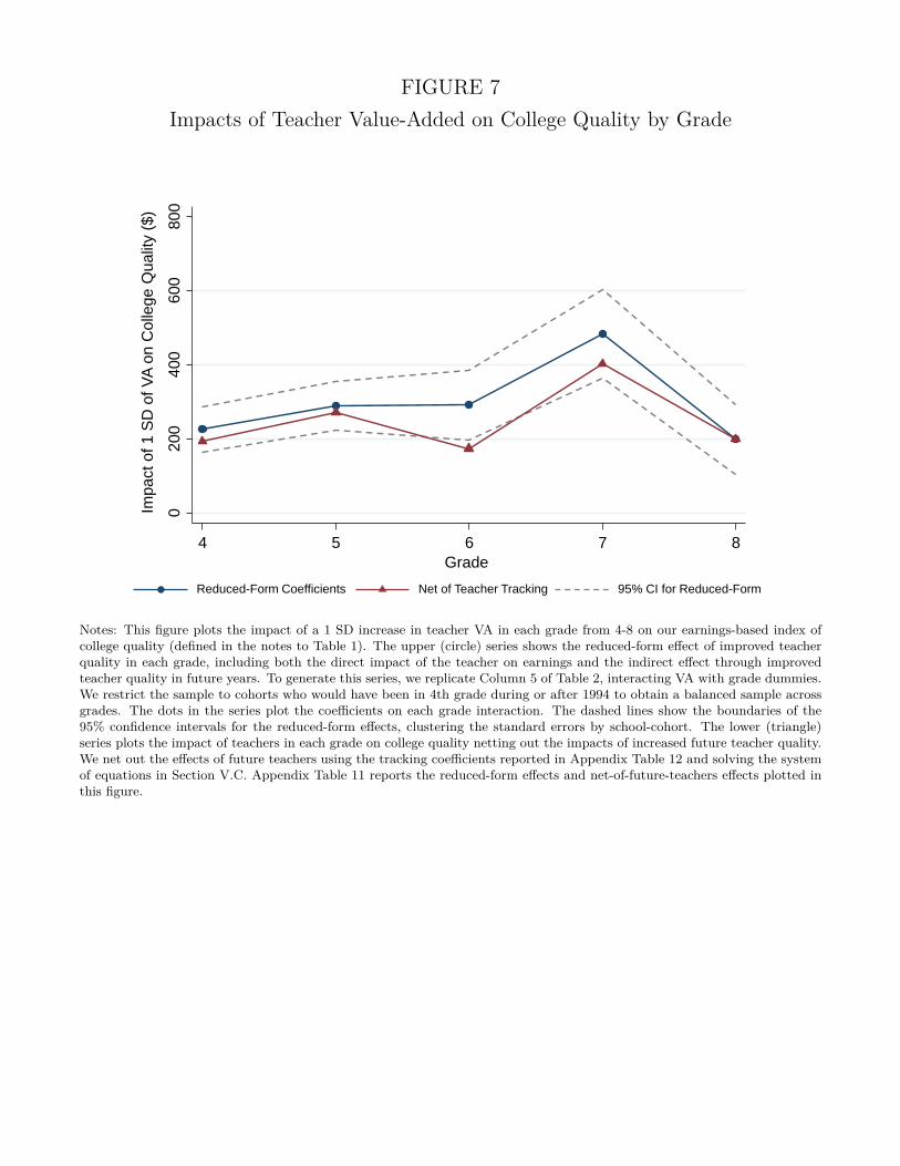
FIGURE 7Impacts of Teacher Value-Added on College Quality by Grade

020

040

060

080

0

4 5 6 7 8

Impa

ct o

f 1 S

D o

f VA

on

Col

lege

Qua

lity

($)

Grade

Reduced-Form Coefficients 95% CI for Reduced-FormNet of Teacher Tracking

Notes: This figure plots the impact of a 1 SD increase in teacher VA in each grade from 4-8 on our earnings-based index ofcollege quality (defined in the notes to Table 1). The upper (circle) series shows the reduced-form effect of improved teacherquality in each grade, including both the direct impact of the teacher on earnings and the indirect effect through improvedteacher quality in future years. To generate this series, we replicate Column 5 of Table 2, interacting VA with grade dummies.We restrict the sample to cohorts who would have been in 4th grade during or after 1994 to obtain a balanced sample acrossgrades. The dots in the series plot the coefficients on each grade interaction. The dashed lines show the boundaries of the95% confidence intervals for the reduced-form effects, clustering the standard errors by school-cohort. The lower (triangle)series plots the impact of teachers in each grade on college quality netting out the impacts of increased future teacher quality.We net out the effects of future teachers using the tracking coefficients reported in Appendix Table 12 and solving the systemof equations in Section V.C. Appendix Table 11 reports the reduced-form effects and net-of-future-teachers effects plotted inthis figure.

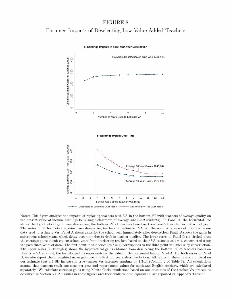
FIGURE 8Earnings Impacts of Deselecting Low Value-Added Teachers

a) Earnings Impacts in First Year After Deselection

Gain from Deselection on True VA = $406,988

010

020

030

040

0

Life

time

Ear

ning

s G

ain

Per

Cla

ss (

$100

0s)

0 2 4 6 8 10

Number of Years Used to Estimate VA

b) Earnings Impact Over Time

Average 10 Year Gain = $184,234

Average 10 Year Gain = $246,744

010

020

030

040

0Li

fetim

e E

arni

ngs

Gai

n P

er C

lass

($1

000s

)

1 2 3 4 5 6 7 8 9 10 11 12 13

School Years Since Teacher Was Hired

Deselected on Estimated VA in Year 4 Deselected on True VA in Year 4

Notes: This figure analyzes the impacts of replacing teachers with VA in the bottom 5% with teachers of average quality onthe present value of lifetime earnings for a single classroom of average size (28.2 students). In Panel A, the horizontal lineshows the hypothetical gain from deselecting the bottom 5% of teachers based on their true VA in the current school year.The series in circles plots the gains from deselecting teachers on estimated VA vs. the number of years of prior test scoredata used to estimate VA. Panel A shows gains for the school year immediately after deselection; Panel B shows the gains insubsequent school years, which decay over time due to drift in teacher quality. The lower series in Panel B (in circles) plotsthe earnings gains in subsequent school years from deselecting teachers based on their VA estimate at t = 4, constructed usingthe past three years of data. The first point in this series (at t = 4) corresponds to the third point in Panel A by construction.The upper series (in triangles) shows the hypothetical gains obtained from deselecting the bottom 5% of teachers based ontheir true VA at t = 4; the first dot in this series matches the value in the horizontal line in Panel A. For both series in PanelB, we also report the unweighted mean gain over the first ten years after deselection. All values in these figures are based onour estimate that a 1 SD increase in true teacher VA increases earnings by 1.34% (Column 2 of Table 3). All calculationsassume that teachers teach one class per year and report mean values for math and English teachers, which are calculatedseparately. We calculate earnings gains using Monte Carlo simulations based on our estimates of the teacher VA process asdescribed in Section VI. All values in these figures and their undiscounted equivalents are reported in Appendix Table 13.

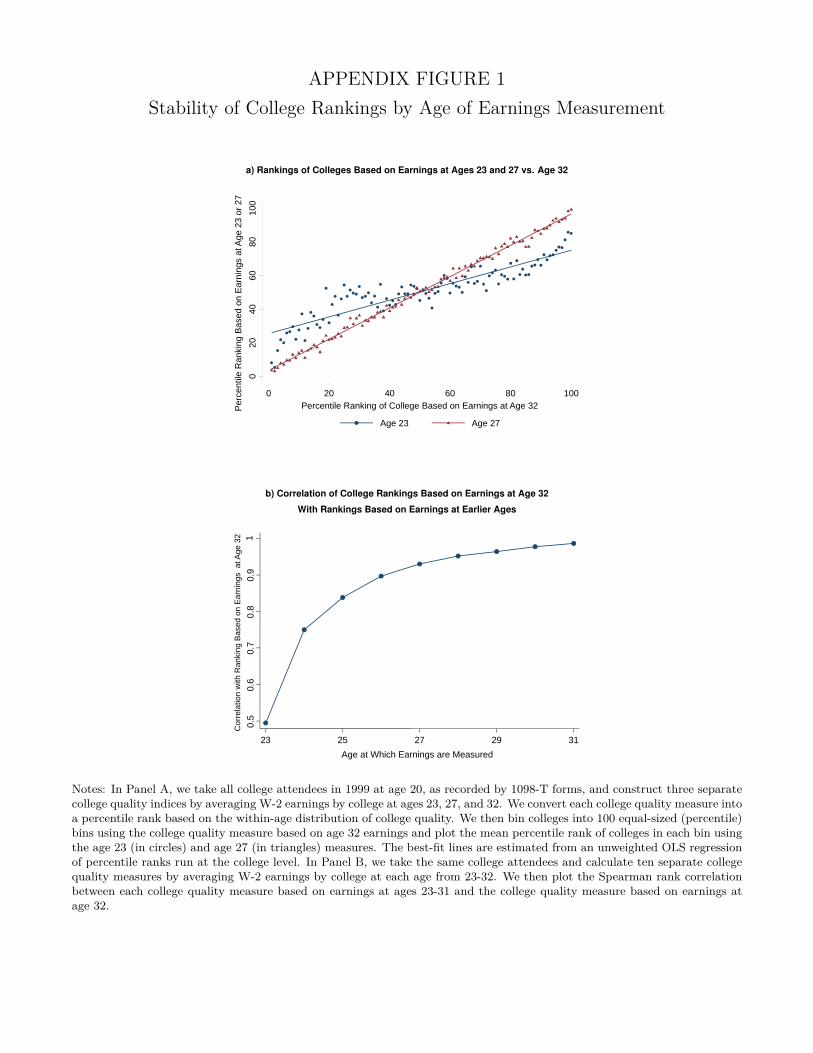
APPENDIX FIGURE 1Stability of College Rankings by Age of Earnings Measurement

a) Rankings of Colleges Based on Earnings at Ages 23 and 27 vs. Age 32

020

4060

8010

0

0 20 40 60 80 100

Per

cent

ile R

anki

ng B

ased

on

Ear

ning

s at

Age

23

or 2

7

Percentile Ranking of College Based on Earnings at Age 32

Age 27Age 23

b) Correlation of College Rankings Based on Earnings at Age 32

With Rankings Based on Earnings at Earlier Ages

0.5

0.6

0.7

0.8

0.9

1C

orre

latio

n w

ith R

anki

ng B

ased

on

Ear

ning

s a

t Age

32

23 25 27 29 31

Age at Which Earnings are Measured

Notes: In Panel A, we take all college attendees in 1999 at age 20, as recorded by 1098-T forms, and construct three separatecollege quality indices by averaging W-2 earnings by college at ages 23, 27, and 32. We convert each college quality measure intoa percentile rank based on the within-age distribution of college quality. We then bin colleges into 100 equal-sized (percentile)bins using the college quality measure based on age 32 earnings and plot the mean percentile rank of colleges in each bin usingthe age 23 (in circles) and age 27 (in triangles) measures. The best-fit lines are estimated from an unweighted OLS regressionof percentile ranks run at the college level. In Panel B, we take the same college attendees and calculate ten separate collegequality measures by averaging W-2 earnings by college at each age from 23-32. We then plot the Spearman rank correlationbetween each college quality measure based on earnings at ages 23-31 and the college quality measure based on earnings atage 32.

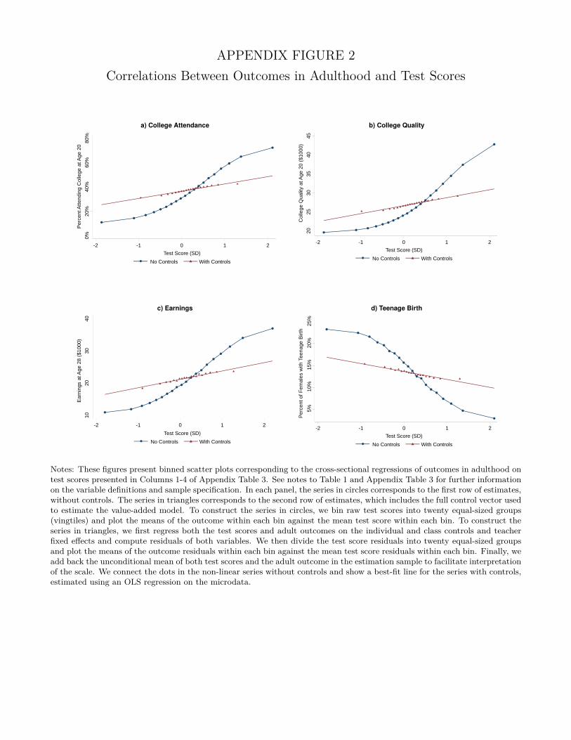
APPENDIX FIGURE 2Correlations Between Outcomes in Adulthood and Test Scores

a) College Attendance

-2 -1 0 1 2

Per

cent

Atte

ndin

g C

olle

ge a

t Age

20


Test Score (SD)

0%20

%40

%60

%80

%

b) College Quality

2025

3035

4045

-2 -1 0 1 2

Col

lege

Qua

lity

at A

ge 2

0 ($

1000

)


Test Score (SD)

c) Earnings

1020

3040

-2 -1 0 1 2


Test Score (SD)

Ear

ning

s at

Age

28

($10

00)

d) Teenage Birth

-2 -1 0 1 2

Per

cent

of F

emal

es w

ithTe

enag

eB

irth


Test Score (SD)

5%10

%15

%20

%25

%

Notes: These figures present binned scatter plots corresponding to the cross-sectional regressions of outcomes in adulthood ontest scores presented in Columns 1-4 of Appendix Table 3. See notes to Table 1 and Appendix Table 3 for further informationon the variable definitions and sample specification. In each panel, the series in circles corresponds to the first row of estimates,without controls. The series in triangles corresponds to the second row of estimates, which includes the full control vector usedto estimate the value-added model. To construct the series in circles, we bin raw test scores into twenty equal-sized groups(vingtiles) and plot the means of the outcome within each bin against the mean test score within each bin. To construct theseries in triangles, we first regress both the test scores and adult outcomes on the individual and class controls and teacherfixed effects and compute residuals of both variables. We then divide the test score residuals into twenty equal-sized groupsand plot the means of the outcome residuals within each bin against the mean test score residuals within each bin. Finally, weadd back the unconditional mean of both test scores and the adult outcome in the estimation sample to facilitate interpretationof the scale. We connect the dots in the non-linear series without controls and show a best-fit line for the series with controls,estimated using an OLS regression on the microdata.

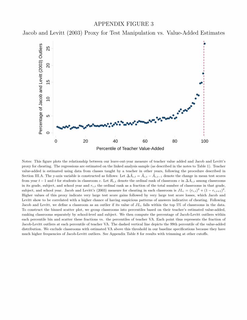
APPENDIX FIGURE 3Jacob and Levitt (2003) Proxy for Test Manipulation vs. Value-Added Estimates

05

1015

2025

Per

cent

age

of J

acob

and

Lev

itt (

2003

) O

utlie

rs

0 20 40 60 80 100

Percentile of Teacher Value-Added

Notes: This figure plots the relationship between our leave-out-year measure of teacher value added and Jacob and Levitt’sproxy for cheating. The regressions are estimated on the linked analysis sample (as described in the notes to Table 1). Teachervalue-added is estimated using data from classes taught by a teacher in other years, following the procedure described inSection III.A. The y-axis variable is constructed as follows: Let ∆Ac,t = Ac,t − Ac,t−1 denote the change in mean test scoresfrom year t− 1 and t for students in classroom c. Let Rc,t denote the ordinal rank of classroom c in ∆Ac,t among classroomsin its grade, subject, and school year and rc,t the ordinal rank as a fraction of the total number of classrooms in that grade,subject, and school year. Jacob and Levitt’s (2003) measure for cheating in each classroom is JLc = (rc,t)2 + (1 − rc,t+1)2.

Higher values of this proxy indicate very large test score gains followed by very large test score losses, which Jacob andLevitt show to be correlated with a higher chance of having suspicious patterns of answers indicative of cheating. FollowingJacob and Levitt, we define a classroom as an outlier if its value of JLc falls within the top 5% of classrooms in the data.To construct the binned scatter plot, we group classrooms into percentiles based on their teacher’s estimated value-added,ranking classrooms separately by school-level and subject. We then compute the percentage of Jacob-Levitt outliers withineach percentile bin and scatter these fractions vs. the percentiles of teacher VA. Each point thus represents the fraction ofJacob-Levitt outliers at each percentile of teacher VA. The dashed vertical line depicts the 99th percentile of the value-addeddistribution. We exclude classrooms with estimated VA above this threshold in our baseline specifications because they havemuch higher frequencies of Jacob-Levitt outliers. See Appendix Table 8 for results with trimming at other cutoffs.

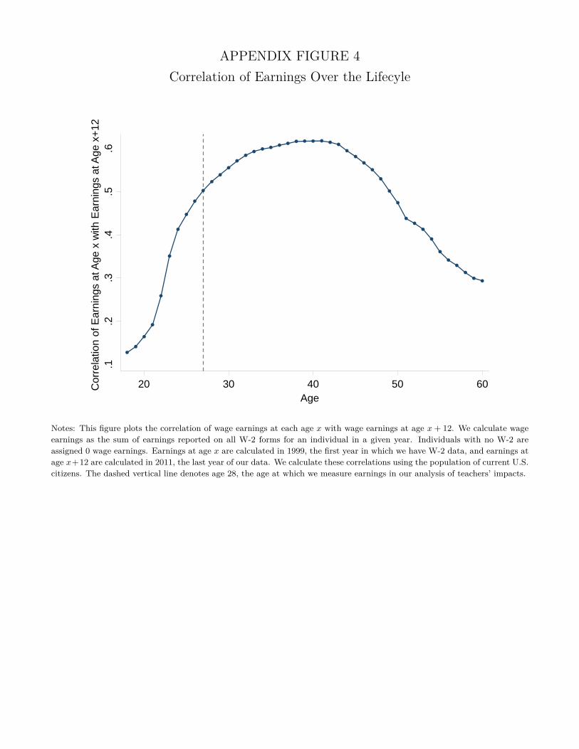
APPENDIX FIGURE 4Correlation of Earnings Over the Lifecyle

.1.2

.3.4

.5.6

Cor

rela

tion

of E

arni

ngs

at A

ge x

with

Ear

ning

s at

Age

x+

12

20 30 40 50 60Age

Notes: This figure plots the correlation of wage earnings at each age x with wage earnings at age x+ 12. We calculate wageearnings as the sum of earnings reported on all W-2 forms for an individual in a given year. Individuals with no W-2 areassigned 0 wage earnings. Earnings at age x are calculated in 1999, the first year in which we have W-2 data, and earnings atage x+12 are calculated in 2011, the last year of our data. We calculate these correlations using the population of current U.S.citizens. The dashed vertical line denotes age 28, the age at which we measure earnings in our analysis of teachers’ impacts.

Measuring the Impacts of Teachers II: Teacher Value-Added ... · Measuring the Impacts of Teachers...

Documents

Transcript of Measuring the Impacts of Teachers II: Teacher Value-Added ... · Measuring the Impacts of Teachers...