Measuring Patient Similarities via A DeepArchitecture with Medical Concept Embedding

Zihao Zhu∗, Changchang Yin∗, Buyue Qian∗, Yu Cheng†, Jishang Wei‡, Fei Wang§∗Xi’an Jiaotong University, Xi’an, Shangxi 710049, China

{zihaozhu,lentery}@stu.xjtu.edu.cnqianbuyue@xjtu.edu.cn

†IBM T. J. Watson Research, Yorktown Heights, NY 10598, USA

chengyu@us.ibm.com‡HP Labs, 1501 Page Mill Rd, Palo Alto, CA 94304, USA

jishang.wei@hp.com§Department of Healthcare Policy and Research, Weill Cornell Medical College, Cornell University

few2001@med.cornell.edu

Abstract—Evaluating the clinical similarities between pairwisepatients is a fundamental problem in healthcare informatics. Aproper patient similarity measure enables various downstreamapplications, such as cohort study and treatment compara-tive effectiveness research. One major carrier for conductingpatient similarity research is the Electronic Health Records(EHRs), which are usually heterogeneous, longitudinal, andsparse. Though existing studies on learning patient similarityfrom EHRs have shown being useful in solving real clinicalproblems, their applicability is limited due to the lack of medicalinterpretations. Moreover, most previous methods assume avector based representation for patients, which typically requiresaggregation of medical events over a certain time period. As aconsequence, the temporal information will be lost. In this paper,we propose a patient similarity evaluation framework based ontemporal matching of longitudinal patient EHRs. Two efficientmethods are presented, unsupervised and supervised, both ofwhich preserve the temporal properties in EHRs. The supervisedscheme takes a convolutional neural network architecture, andlearns an optimal representation of patient clinical recordswith medical concept embedding. The empirical results on real-world clinical data demonstrate substantial improvement overthe baselines.

Index Terms—Patient Similarity, Deep Matching, MedicalConcept Embedding

I. INTRODUCTION

Patient similarity learning has been identified as one of the

key techniques for healthcare transformation. During the past

decade, Electronic Health events (EHRs), including diagnosis

codes, lab results, prescription data, are becoming readily

available for a huge amount of patients. This makes EHRs

a valuable resource for evaluating the clinical similarities

between pairwise patients. Patient similarity, which measures

how similar a pair of patients are according to their historical

information under a specific clinical context, will be the

enabling technique for making various healthcare applica-

tions possible, such as cohort analysis, case based reasoning,

treatment comparison, disease subtyping, and personalized

medicine. In addition, learning patient similarity is a funda-

mental problem in evidence based medicine, which has been

identified as one of the major thrust areas for transforming

healthcare and improving the quality of delivery of care.

Motivation. One of the key challenges to derive patient

similarity measure is how to represent the medical events of

patients effectively without loss of information. Since a great

deal of healthcare analytics applications critically rely upon

patient similarity, the similarity measures need to be both clin-

ically effective and accurate. Though important, there are only

a handful studies on patient similarity learning [1] [2]. Existing

methods have successfully derived the similarity measure from

EHRs data through mapping the medical events into vector

spaces, however, their applicability is limited due to the lack of

convincing explanations for patient representations in medical

domain. There has been some existing work on applying

patient similarity to various applications in medical literatures.

However, there are still significant challenges on learning

effective patient similarities, which, to our knowledge, have

not been systematically addressed. (i) Temporal-Sensitivity:Temporal information is important to medical events, and is

crucial to understand the dynamics of medical expressions.

(ii) High Dimensionality and Sparsity: EHRs includes a wide

range of data (such as diagnosis, medication, lab test) and a

large number of possible medical events (over ten thousands

of diseases and medications), so that EHRs data is usually

represented in a high dimensional space. Besides, EHRs data is

also very sparse, since a record exists if and only if the patient

pays a visit to a specific clinical institute, for a particular

condition. (iii) Limited interpretability: Due to the complexity

of medical data, existing patient representation models are

often weak at the perspective of clinical interpretations, which

if addressed would significantly widen their applicability.

Proposal. Taking into account all challenges mentioned

above, inspired by the idea of words embedding [3], we

propose a method to represent patients and derive a similarity

measure based on it. Unlike previous methods that model

each medical event as a binary event vector over time (one

if the medical event happened and zero otherwise), we derive

2016 IEEE 16th International Conference on Data Mining

2374-8486/16 $31.00 © 2016 IEEE

DOI 10.1109/ICDM.2016.90

749

a fixed-length vector representation from EHRs by medical

concept embedding. In text mining, a particular word can be

predicted based on the context around it [4] [3]. Similarly,

events happened before and after a specific medical event

can be viewed as its medical context, which may be used

to make event predictions in medical domain. Based on the

medical context, each event is compressed into a given length

vector with medical concept embedding. Similar to the word

embedding [3], the event embedding presented in our model

hold its natural medical concept. Furthermore, we adjust the

range of context, with respect to the specific conditions of a

medical event, to achieve an event embedding with temporal

information. By stacking all event embedding vectors together,

each patient is then represented as an embedding matrix.

Note that, compared to describing patients using binary event

vectors, the embedding extracts clinical features of a patient

from EHRs and represent them in a reasonable dimension,

resulting a natural dense embedding matrix for every patient.Based on the embedding matrix representation of patients,

we propose two methods, supervised and unsupervised, to de-

rive the similarity measures. Note that the number of medical

events varies from patients to patients, and both the supervised

and unsupervised approaches are required to measure the

similarity between matrices with different dimensions. As for

the unsupervised method, we adopt the RV coefficient [5]

and dCov coefficient [6], respectively, to measure linear and

non-linear relations between pairwise patients based on the

embedding matrix. In the supervised model, we measure the

patients similarity using the Convolutional Neural Network

(CNN), where the deep medical embedding is obtained from

the intermediate convolutional feature maps. With the given

number of convolutional filters, an event embedding matrix

is mapped to a fixed-length feature vector. The deep medical

concept embedding contributes to improved patients similarity

measures. We shall later in the paper make a comparison

amongst different types of patient representations, including

the binary event matrix representation.Empirical Study. Patient cohort study is the most effective

way to analyze the causes, treatments, and outcomes of

diseases. To evaluate the representations we proposed, we

conduct a cohort analysis based on the obtained measures of

patient similarity. Our model is tested on a real-world EHRs

dataset containing a wide range of medical events over a

long time period. The experimental results demonstrate the

effectiveness of our model in measuring patient similarity.Contributions. Our work makes the following distinctive

technical contributions:

• We adopt a state-of-the-art distributional representation

model to project medical events to fixed-length vectors,

which are then used to measure patient similarity.

• We effectively extract the low-dimensional and dense

representation for patients from EHR data, with the

temporal information preserved.

• We propose two solutions for patient similarity Learning,

unsupervised and supervised. This makes our frame-

work applicable to most similarity-related applications in

healthcare analytics.

The rest of this paper is organized as follows. Section

II introduces related studies. Details about our model are

presented in Section III. The experimental results are reported

in Section IV, and Section V concludes.

II. RELATED WORK

In this section, we first review some related work on

evaluating the clinical patient similarities, and then review

some relevant problems associated with deep learning.

A. Patient Similarity

In healthcare informatics domain, there are a lot of works

focusing on patient similarity. For example, [7] proposed a

patient similarity algorithm named SimSvm that uses Support

Vector Machine(SVM) to weight the similarity measures. [8]

proposed a patient similarity based disease prognosis strategy

named SimProX. This model uses a Local Spline Regression

(LSR) based method to embed these patient events into an

intrinsic space, then measure the patient similarity by the

Euclidean distance in the embedded space. These methods

do not take the temporal information into consideration when

evaluating patient simiarities. Wang [9] presented an One-

Sided Convolutional Matrix Factorization for detection of

temporal patterns. Cheng [1] proposed an adjustable tem-

poral fusion scheme using CNN-extracted features. Based

on patients similarity, plenty of applications are enabled. In

[10], Ng provided personalized predictive healthcare model

by matching clinical similar patients with a locally supervised

metric learning measure. [11] proposed Integrated Method

for Personalised Modelling (IMPM) to provide personalised

treatment and personalised drug design.

There are many research have been conducted on clustring

patients based on machine learning. In order to rate patients

health perceptions, Sewitch [12] make cluster analysis using k-

means to identify the patients groups based on the discovering

the multivariate pattern. To capture underlying structure in the

history of present illness section from patients EHRs, Henao

[13] proposed a statistical model that groups patients based

on text data in the initial history of present illness (HPI) and

final diagnosis (DX) of a patients EHRs. For human disease

gene expression, Huang [14] presented a new recursive K-

means spectral clustering method (ReKS) to efficient cluster

human diseases. Most of these research have demonstrate

effectiveness of their model with real-world experiments, that

convinces us of the applicability of clustering patients on

cohorts discovering.

B. Embedding Learning and Semantic Matching

One of the most important components in our patients

similarity measure is deep distributional medical concept

embedding. Distributional representations has gone through

the long evolution, and shows state-of-the-art results in many

fields recently. [3], [4] proposed continuous Bag-of-Words

model and Skip-gram model to represent words in vector

750

space. The word representations using neural networks pro-

vide state-of-the-art performance on measuring syntactic and

semantic word similarities. Many works as well as ours are

inspired by the words embedding with neural networks. [15]

learned image embedding by concatenating skip-gram linguis-

tic representation vectors with visual concept representation

vectors. [16] encoded a query-document pairs into discriminate

feature vectors using distributional sentence model. Our model

achieves the goal of embedding patients clinical features in the

dense matrices with modest dimensionality.

With medical concept embedding, we look forward to

calculating the similarity amongst patients according to their

EHRs. Considering the representations of patient medical

events do not have a common time dimension, we cannot

compare the patient event matrix directly. [17] provided a

relevant similarity measures between temporal series of brain

functional images belonging to different subjects. Similar to

[17], we adopt the RV coefficient to measure patient similari-

ties. Note, however, that this coefficient only considers linear

relationships between two data sets. To do more systematic

research on measuring similarity of patient, our model also

measures non-linear correlation between two patients using

dCov coefficient. Apart from those unsupervised approach, we

adopt the supervised learning method. We modify the Convo-

lutional Neural Network(CNN) to derive the similarity scores

for pairs of patients. The Convolutional networks models

which are originally invented for image processing have wide

applications in other domains. [16], [18] and [19] respectively

obtains the continuous representations of the sentences or short

texts by a convolutional deep network, then the similarity can

be effectively established.

III. THE PROPOSED METHOD

Accessing patients similarities in EHRs data is a very

challengeable task. In this section, we will fist propose to

learn the contextual embedding of each medical concept.

Then we provide an unsupervised method to estimate the

similarity score, which takes the learned medical concept as

the input. After that we exploit an architecture building with

convolutional neural network to measure the similarity of pair

patient records with some supervision encoded.

A. Contextual Embedding of Medical Concepts

Our goal in this step is to get the contextual embedding

of each medical concept from patient EHRs, which provide a

better representation for medical concepts than general one-

hot encoding representation. By “context around a medical

concept A we really mean the medical events happening

before and after A within the patient EHRs corpus. For each

patient, by concatenating all medical events in his/her EHRs

according to their happening timestamps (for events with the

same timestamp we do not care about the order), we obtained a

paragraph describing the historical condition of him/her. So the

context around a specific medical event is similar to the context

around a word in a paragraph. How to derive effective word

representations by incorporating contextual information is a

fundamental problem in Natural Language Processing (NLP)

and has been extensively studied. One recent advance is the

Word2Vec technique [4] that trains a two-layer neural network

from a text corpus to map each word into a vector space

encoding the word contextual correlations. The similarities

(usually cosine distance) evaluated in such embedded vector

space reflect the contextual associations (e.g., words A and B

with high similarity suggests they tend to appear in the same

context).In NLP, the context around each word is usually identified

as the adjacent words before and after it. In Word2Vec such

context is defined by a sliding window around each word

and the length of the window reflects the scope of the

context. In EHRs, as there is a timestamp associated with

each medical concept, we do not just want to consider the

relative positions when defining the context, but consider the

actual timestamps. For example, we may want to treat event

B happened one year after A differently comparing to event

B happened one week after A. Another factor we need to

consider is the context scope around each event, i.e., the

length of the sliding windows. In Word2Vec models for NLP

every word is assigned with the same window length. In

contrast, for EHRs, we may want medical concepts related to

chronic conditions to have larger scopes while acute condition

concepts to have smaller scopes. Moreover, because of the

variabilities among individual patients, the scope for the same

event could be different for different patients. Therefore we

propose an adaptive way to determine the window length for

an event in the EHRs of a specific patient. Our heuristic is

that chronic conditions are more likely to appear repeatedly

in a patients EHRs and thus have higher frequency, and acute

conditions will be less frequent. Then for medical event i and

patient p,

L(i, p) = f(i, p) ∗ a+ θ (1)

where f(i, p) is the frequency of event i in the EHRs of patient

p. a and θ are constants.

B. Temporal Patient RepresentationAfter the medical concepts embedding step, We expect

that the medical concept representations learned by Skip-gram

will show similar properties so that the concept vectors will

support clinically meaningful vector additions. A straitfoward

representation of a patient p will be as simple as convert-

ing all medical concepts in his medical history to medical

concept vectors, then summing all those vectors to obtain a

single representation vector. However, this representation will

loss the temporal information. Instead, we utilize a temporal

representation: the records of each patient p is represented

as a matrix X with dimension d × Np, where d is the fix

embedding dimension and Np is the total number of visit

patient p has. A single representation vector of one visit is

obtained by summing all the medical vectors in that visit.

Usually, Np varies from patient to patient. Given two patients

pa and pb, calculating the similarity between the record Xa

and Xb is not that intuitive. We propose the method in the

following sections.

751

Figure 1: The overall framework of supervised patient similarity matching. To train the singular neural network, embedding

matrices of pairs of patients Ea,Eb passed through convolutional filters are mapped into feature maps. We build the deep

embedding patients representations Pa,Pb for patients by pooling patients feature maps into the intermediate vectors. With the

rich feature vectors we learn a symmetrical similarity matrix M for measuring the distance between patient a and b.

C. Unsupervised Patient Similarity

In order to calculate the similarity score based on the patient

temporal representation, we provide two alternatives. The first

one is to utilize RV coefficient [] and dCov efficient to estimate

the similarity over the pair of temporal patient representation.

In particularly, given two matrix representations X ∈ Rn×k

and Y ∈ Rm×k, the RV coefficient is defined as:

RV(X,Y) =tr(XX‘YY‘)√

tr(XX‘)2tr(YY‘)2(2)

For the dCov efficient, let’s first define the empirical dis-

tance covariance:

dCov2n(X,Y) =1

n2

n∑i,j=1

(dXij−dXi.−dX.j+dX.. )(dYij−dYi.−dY.j+dY.. )

(3)

where dij() is the Euclidean distance between sample i and

j of random vector xi, di. =1n

∑nj=1 dij , d.j =

1m

∑ni=1 dij ,

d.. =1n

∑m,ni,j=1 dij . The empirical distance correlation (dCov

efficient) is defined:

dCor2n(X,Y) =dCov2n(X,Y)√

dCov2n(X,X)dCov2n(Y,Y)(4)

D. Measure Similarities with Supervision

In order to add some supervision to this procedure, we

proposed a deep learning model. The idea is derived from

semantic matching problem in NLP, which aims to determine

a matching score for two given texts. Deep learning approach

has been applied to this area and most of the models con-

ducts the matching through creating a hierarchical matching

structure built on convoluational neural nets (ConvNets). The

architecture of our model for measure patient pairs is presented

in Figure 1. The models based on ConvNets learn to map input

patient representation to vectors, which can then be used to

compute their similarity. These are then used to compute a

patient similarity score, which together with the representation

vectors are joined in a single representation.

In the following we describe how the intermediate repre-

sentations produced by the ConvNets model can be used to

compute patient similarity scores and give a brief explanation

of the remaining layers, e.g. hidden and softmax, used in our

network.

Single Convolution feature maps: The aim of the convolu-

tional layer is to extract effective patterns, i.e., discriminative

medical concept sequences found within the input record that

are common throughout the training instances. In general, let

xi ∈ Rd be the d-dimensional event vector corresponding to

the i-th time items. A one-side convolution operation involves

a filter w ∈ Rd×h, which is applied to a window of h event

features to produce a new feature. For example, a feature ciis generated from a window of events xi:i+h−1 is defined by:

ci = f(w � xi:i+h−1 + b) (5)

where b ∈ R is a bias term and f is a non-linear function (we

use rectification (ReLU)).

Pooling: The output from the convolutional layer (passed

through the activation function) are then passed to the

pooling layer, whose goal is to aggregate the informa-

tion and reduce the representation. This filter is applied

to each possible window of features in the event matrix

{x1:h, x2:h+1, ..., xn−h+1:n} to produce a feature map c =[c1, c2, ..., cn−h+1], where c ∈ R

n−h+1. We then apply a

max pooling over the feature map and take the average value

c = max{c}. The idea is to capture the most important feature

one with the highest value for each feature map.

752

Matching Matrix: Given the output of our basic for pro-

cessing patient records, their resulting vector representations

xa and xb, can be used to compute a record-record similarity

score. We follow the approach of [20] that defines the simi-

larity between xa and xb vectors as follows:

sim(xa,xb) = xTa MxT

b (6)

where M ∈ Rm×m is a similarity matrix. The similarity

matrix M is a symmetrical parameter of the network and is

optimized during the training.

Softmax: The output of the penultimate convolutional and

pooling layers is flattened to a dense vector x, which is passed

to a fully connected softmax layer. It computes the probability

distribution over the labels.

E. Optimization

For different tasks, we need to utilize different loss functions

to train our model. Taking regression as an example, we can

use square loss for optimization:

L(S1, S2, y) = (y −M(S1, S2))2 (7)

where y ∈ R is the real-valued ground-truth label to indicate

the matching degree between S1 and S2.

All parameters of the model, including the parameters of

word embedding, neural tensor network, spatial RNN are

jointly trained by BackPropagation and Stochastic Gradient

Descent. Specifically, we use AdaGrad [21] on all parameters

in the training process.

Regularization For regularization we employ dropout on

the penultimate layer. Dropout prevents co-adaptation of hid-

den units by randomly dropping outi.e., setting to zeroa pro-

portion p of the hidden units during fowardbackpropagation.

IV. EXPERIMENTS AND EVALUATION

In this section, we evaluate our framework on a real

clinical EHRs dataset. We carry out the cohort studies by

selecting several chronic diseases associated with a range of

comorbidities. There are some reasons for our cohort selection.

First, they are frequently occurred diseases being extensively

analyzed in healthcare applications. Second, these diseases

are highly associated with each other, and their combination

presents many diagnostic challenges. More importantly, due

to the long period progression path of those disease, there are

a great deal of temporal information embedded in the medical

events. Many of medical research based on machine learning

ignored the temporality while our model effectively extract

those features and enrich the patients representations. Based on

patients clinical similarities derived from these representations,

we group patients into clusters by some classical clustering

algorithms. As we focus on matching similar patients, the

clustering evaluations verify the effectiveness of our model.

As testing our model on the real world EHRs, we demon-

strate that our method can effectively represent patients with-

out sacrificing temporal information. With the distributional

continuous representations, we apply deep neural networks to

derive measure of similarities amongst patients in the datasets.

We then make use of the similarity matrix to group patients.

For the evaluations shown in the results, we are convinced

that the deep medical event embedding achieves a significant

improvement in patients representations.

Further more, we demonstrate the robustness of our model

in the cohort studies. As mentioned in [22], the primary

disadvantage of medical cohort study is the limited control

the investigator has over data collection. The existing data

may be incomplete, inaccurate, or inconsistently measured

between subjects [23]. As a result, we process patients EHRs

for constructing two kinds of data sets. One covers the whole

complete patient events for global features analyzing. On

another data set, we remove particular events labeled as cohort

identifers from patients EHRs to provide more natural setting

in clinical cases. We systematically analyze the performance

of our model in the above two settings, and draw some

conclusions through our result discussions.

A. Datasets

Our model is trained on a real world longitudinal EHRs

database of 218,680 patients for the course of over four years.

According to the reasons presented at the beginning of this

section, we select four patient cohorts from the EHRs data,

namely, Chronic Obstructive Pulmonary Disease (COPD),

Diabetes, Heart Failure, and Obesity.

Table I provides a summary of the patient cohorts used in

our experiment. Each cohort consists of a set of case patients

who are confirmed with one of the four diseases according to

their medical diagnosis, and each patient comes with a set of

medical events including diagnosis and medications. In each

patient encounter, we use the International Classification of

Disease-Version 9 (ICD-9) codes to denote the diagnosis of

diseases that a patient suffers from. All the clinical events

about medications are pre-processed to normalize the descrip-

tions based on brand names and clinical dosages.

Cohorts # Patients # Events

COPD 2,000 247,043Diabetes 2,000 259,074Obesity 2,000 211,496Heart Failure 1,135 165,254

Total 7,135 882,867

Table I: Summary of EHRs datasets for patients clustering.

We construct datasets with medical events collected from

patients who were confirmed of having the disease by medical

experts. We develop the criteria that any patients presented

in the datasets has at least forty events. The requirement

is set to ensure that each test case has minimum events of

clinical history that could be used in reasonable analytics

tasks in healthcare. Also, to enable distinctly cluster without

overlapping among cohorts, we remove patients who suffers

from more than one disease in the cohort list. Finally, there

are 8,000 remaining patients and 6,064 distinct clinical events.

Medical event appearing in more than 90% of patients or

753

present in fewer than five patients are removed from the

datasets to avoid biases and noise in the learning process.

In the following experiments, we use two datasets:

DATASET-I uses the complete patients events while

DATASET-II reserves historical events except those labeled

as cohort identifiers. On DATASET-I, we split the dataset into

training and test sets with same number of patients, and other

patients left for validation. As for DATASET-II, we construct

the data sets in accordance with DATASET-I. A few of patients

are filtered out because of the limited number of their medical

events. Table II summaries the two datasets.

Data # Patients # Events

DATASET-ITRAIN 3,211 396,072TEST 3,210 399,804DEV 714 86,991

DATASET-IITRAIN 3,083 373,145TEST 3,080 377,287DEV 685 81,392

Table II: Summary of modeling datasets.

B. Medical concept embeddings

We use word embeddings to represent each medical event

as a vector. We run word2vec on the datasets containing

218,680 patients with around 16.9 million medical event

records. To learn the embeddings, we choose the Bag of Words

model with window size setting to 20 and events filtering with

frequency less than 5. The dimensionality of our embedding

vectors d is set to 20, 30, 50, 200, 500, respectively, for the

comparison purpose, and after a serial practices we select 50

as medical event dimension according to the best performance.

Finally, the resulting event matrix covers around 8,000 events

which are presented using 50-dimensional vectors, and the

event matrix contains all of medical features of patient. Next,

we shall discuss how to use them for representing individuals

and measuring their distances.

C. Experimental Settings

The parameters of our deep learning were as follow: the

width of the convolution filters w is set to 5, 10, 15, 20,

25, and the number of convolutional feature maps m takes

on 50, 100, 150, 200. We use stochastic gradient descent

to optimize the model’s parameters. We train the model

with 50 examples of shuffled mini-batches. We adopt non-

linear rectification (ReLU) activation function and a simple

max-pooling to achieve the intermediate representations. With

regards to overfitting issue we add dropout regularization with

dropout rate setting to 0.5.

To optimize our deep features embedding, we conduct

experiments using several different parameters sets θ ={d, w,m}, which vary in size of word2vec embedding di-

mension, convolution filters width, and the number of convolu-

tional feature maps. In order to find optimal set of parameters,

we compare the performance of clustering with only one

variable of d,w,m varies.

We implement the clustering base on following represen-

tations: (1) One-hot representation. Patient is represented as

an event matrix. The matrices are composed of medical event

columns, the dimension of which is set to 8,000, or the number

of distinct medical events. The event matrix is naturally

sparse, but it simplifies patients descriptions. (2) “Shallow”

embeddings. As described in section IV-B, we make progress

in patients representations with medical event embedding by

word2vec. Similar to One-hot representation, we represent

patients as matrices, but denser and lower dimensional. The

dimension of matrix columns has been reduced, with setting

from 50 to 800. (3) Deep embeddings. To achieve a deep

representation, we combine CNN with distributional medical

events embeddings from word2vec. Based on above event

matrix representations, patients features are filtered through

the convolutional layer of neural network. Feature maps that

represent patients clinical characteristics are then used to

measure patients distances.

With generated representations of each patient, we firstly

calculate the similarity amongst all the test patients. Then, we

group patients cohorts by matching pairs of patients according

to their similarity. Kmeans and Active PCKMeans [24] are

adopted for grouping patients based on the first two repre-

sentations. Also, we compare our model with another metric

learning algorithm that have shown state-of-the-art results in

clustering. Besides deep neural networks we have applied to

learn patients features, we present other two unsupervised

methods for calculating patients distances as complementary.

Specifically, we use RV and dCov coefficient to calculate

correlations of patient feature matrices what derived form

word2vec embedding.

We varify the cohort discover studies by evaluating the

clustering using three popular criteria: Rand index , Purityand normalized mutual information(NMI ).Rand index is frequently used in data clustering, it is

computed as following in [25]:

RI = (TP + TN) /

(n

2

)

where TP counts the number of right decision we have made

on grouping pairs of patients who are in the same cohort into

one cluster, TN is the number of pairs of patients who came

from different cohorts are grouped into dissimilar categories.

In general, bad clusterings have RI values close to 0, a perfect

clustering has a RI of 1.

Purity is one of primary validation measure to evaluate the

cluster quality. We compute Purity as defined in [26]:

Purity (Cluster, Cohort) =1

N

∑I

maxj|pi ∩ qj |

where Cluster = {p1, p2, ..., pI} is the set of clusters,

Cohort = {q1, q2, ...qJ} is the group of classes, or cohorts in

our case. The cohort is identified by the categories of dominant

patients in cluster. Similar to Rand index, the Purity has

upper bound of 1 corresponding to the perfect match between

the partitions and lower bound of 0 that indicates the opposite.

754

NMI measures the information shared by the two cluster-

ings,thus can be adopted as a clusterings similarity measure.

We follow the form defined in [27] to calculate NMI value.

NMI (Cluster, Cohort) =I (Cluster, Cohort)

[H (Cluster) +H (Cohort)] /2

where,

I (X,Y ) =∑x∈X

∑y∈Y

p (x, y) logp (x, y)

p (x) p (y)

is the mutual information between the random variables Xand Y ,

H (X) = −∑x∈X

p (x) log p (x)

is the information entropy of a discrete random variableX .

p (x) , p (x, y) are the probabilities of a object being in cluster

X and in the the intersection of X and Y . The NMI has a

fixed lower bound of 0 and upper bound of 1. In our case,

NMI (Cluster, Cohort) takes its maximum value of 1 when

grouping clusterings are identical to the real cohorts, if the

partition found is totally independent of the real cohorts, then

NMI (Cluster, Cohort) = 0.

There are other popular measures for cluster evaluation,

namely, Precision [28], Recall, and F −measure [29]. We

also validate results by these evaluation.

D. Results and discussion

1) Performance Comparison: Table III summaries the re-

sults of clustering. As we can see, the deep model with feature

embedding is clearly superior to others. On DATASET-I, the

deep embedding model achieves an average Rand index of

0.9887, comparing with the second best one with 0.6796.

Measured by Purity and NMI , it can achieve the per-

formances of 0.9882 and 0.9516, separately, which also

outperforms others with a margin. The superiority of the

model is illustrated in DATASET-II as well, which is a

more difficult task. Measured by Purity and NMI , KMeans1

and Active PCKMeans1 achieve 0.3367, 0.0351 and 0.4410,

0.0682 separately. KMeans2 and Active PCKMeans2 can only

improve 11% and 25% on Purity respectively. However, our

CNN model achieves more than 50% improvement over them.

As a reasonal explanation, we hold that the deep features

learning can be viewed as a two-stage model. During the first

stage, the clinical features of each patients are summarized

in the shallow word2vec embeddings, making progress with

nearly 10% improvement. Next, global features are learned

base on local context features came from word2vec. The

deep learning representation makes continuous improvement,

which leads to a ultimate expression of patients. Figure 2

shows how expressive representations of patients contribute to

match patients cohorts. With a significant 48% improvement

produced, we illustrate the effectiveness of our deep embed-

ding model in expressively representing patients.

One-hot Word embedding Deep embedding

Paitents representations

0.0

0.2

0.4

0.6

0.8

1.0

RandIndex

DATASET-I

DATASET-II

(a)

One-hot Word embedding Deep embedding

Paitents representations

0.0

0.2

0.4

0.6

0.8

1.0

Purity

DATASET-I

DATASET-II

(b)

One-hot Word embedding Deep embedding

Paitents representations

0.0

0.2

0.4

0.6

0.8

1.0

Norm

alizedMutualInform

ation

DATASET-I

DATASET-II

(c)

Figure 2: Performance of different representations.

2) Parameters Optimization: Figure 3 illustrates the opti-

mizations of hyperparameters in our model. The line charts

in one row assess what effects the variation has on grouping

patients. As results summarized in Figure 3a, Figure 3b,

Figure 3c, the dimension of medical event embedding have

little effect on DATASET-I. That because our deep learning

model have successfully obtained the primary features in

the patients representations, achieving nearly perfect 1 of

RI , Purity, and NMI . We make determinations based on

DATASET-II. According to the performance lines shown in the

figures, three clustering evaluations we choose—RI , Purityand NMI achieves the best performance at the same time,

with 50 dimensionality embedding, 100 feature maps, and

755

100 200 300 400 500

Dimension of Word Embeddings

0.5

0.6

0.7

0.8

0.9

1.0

RandIndex

DATASET-Ⅰ

DATASET-Ⅱ

(a)

100 200 300 400 500

Dimension of Word Embeddings

0.5

0.6

0.7

0.8

0.9

1.0

Purity

DATASET-Ⅰ

DATASET-Ⅱ

(b)

100 200 300 400 500

Dimension of Word Embeddings

0.0

0.2

0.4

0.6

0.8

1.0

Norm

alizedMutualInform

ation

DATASET-Ⅰ

DATASET-Ⅱ

(c)

50 100 150 200

Number of Convolution Feature Maps

0.5

0.6

0.7

0.8

0.9

1.0

RandIndex

DATASET-Ⅰ

DATASET-Ⅱ

(d)

50 100 150 200

Number of Convolution Feature Maps

0.5

0.6

0.7

0.8

0.9

1.0

Purity

DATASET-Ⅰ

DATASET-Ⅱ

(e)

50 100 150 200

Number of Convolution Feature Maps

0.0

0.2

0.4

0.6

0.8

1.0

Norm

alizedMutualInform

ation

DATASET-Ⅰ

DATASET-Ⅱ

(f)

2 4 6 8 10 12 14

Width of Convolution Filters

0.5

0.6

0.7

0.8

0.9

1.0

RandIndex

DATASET-Ⅰ

DATASET-Ⅱ

(g)

2 4 6 8 10 12 14

Width of Convolution Filters

0.5

0.6

0.7

0.8

0.9

1.0

Purity

DATASET-Ⅰ

DATASET-Ⅱ

(h)

2 4 6 8 10 12 14

Width of Convolution Filters

0.0

0.2

0.4

0.6

0.8

1.0

NormalizedMutualInformation

DATASET-Ⅰ

DATASET-Ⅱ

(i)

Figure 3: Results on the hyperparameters optimizations. (a), (b), (c) together varify the effect of word embedding dimension

on clustering performance. (d), (e), (f) measures the efficacy of variation on convolution feature maps. (g), (h), (i) make

determinations of convolution feature filters width.

DATASET-I DATASET-IIMethod RI Purity NMI RI Purity NMI

KMeans1 0.5919 0.3538 0.0481 0.5834 0.3367 0.0351Active PCKMeans1 0.6506 0.4801 0.0976 0.6451 0.4410 0.0682KMeans2 0.6627 0.4192 0.1336 0.6547 0.4129 0.1106Active PCKMeans2 0.6796 0.5610 0.1682 0.6794 0.5487 0.1622Matric Learning 0.6732 0.5103 0.1049 0.6475 0.4013 0.1055

Our model(RV ) 0.6679 0.4457 0.2301 0.6285 0.3858 0.1037Our model(dCov) 0.6708 0.4475 0.2361 0.6268 0.3858 0.1048Our model(CNN) 0.9887 0.9882 0.9516 0.7491 0.6894 0.4624

Table III: Evaluations of cohort discovering on DATASET-I, DATASET-II. KMeans1, Active PCKMeans1 groups patients with

One-hot representations, where KMeans2, Active PCKMeans2 adopt the Shallow embeddings to match similar patients pairs.

We contrast the performance of our model at DATASET-I, DATASET-II with the same parameters. Values of RI ,Purity,NMIpresented in the table are average of a group of results.

756

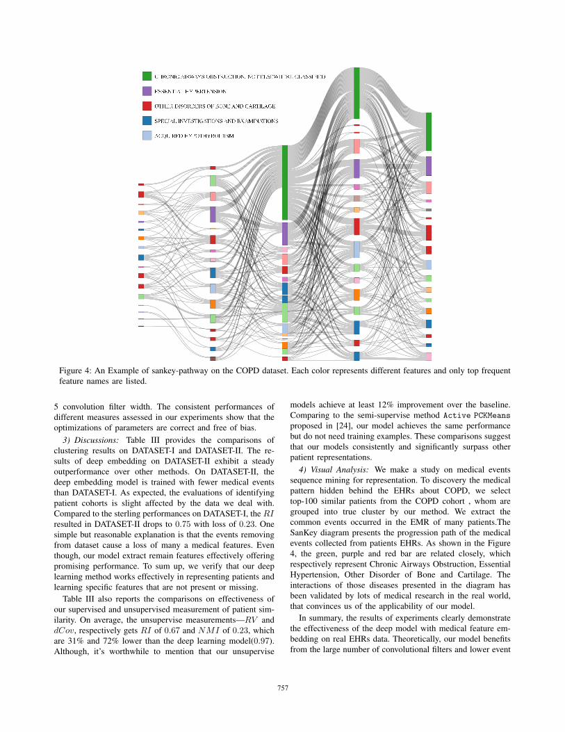
Figure 4: An Example of sankey-pathway on the COPD dataset. Each color represents different features and only top frequent

feature names are listed.

5 convolution filter width. The consistent performances of

different measures assessed in our experiments show that the

optimizations of parameters are correct and free of bias.

3) Discussions: Table III provides the comparisons of

clustering results on DATASET-I and DATASET-II. The re-

sults of deep embedding on DATASET-II exhibit a steady

outperformance over other methods. On DATASET-II, the

deep embedding model is trained with fewer medical events

than DATASET-I. As expected, the evaluations of identifying

patient cohorts is slight affected by the data we deal with.

Compared to the sterling performances on DATASET-I, the RIresulted in DATASET-II drops to 0.75 with loss of 0.23. One

simple but reasonable explanation is that the events removing

from dataset cause a loss of many a medical features. Even

though, our model extract remain features effectively offering

promising performance. To sum up, we verify that our deep

learning method works effectively in representing patients and

learning specific features that are not present or missing.

Table III also reports the comparisons on effectiveness of

our supervised and unsupervised measurement of patient sim-

ilarity. On average, the unsupervise measurements—RV and

dCov, respectively gets RI of 0.67 and NMI of 0.23, which

are 31% and 72% lower than the deep learning model(0.97).

Although, it’s worthwhile to mention that our unsupervise

models achieve at least 12% improvement over the baseline.

Comparing to the semi-supervise method Active PCKMeans

proposed in [24], our model achieves the same performance

but do not need training examples. These comparisons suggest

that our models consistently and significantly surpass other

patient representations.

4) Visual Analysis: We make a study on medical events

sequence mining for representation. To discovery the medical

pattern hidden behind the EHRs about COPD, we select

top-100 similar patients from the COPD cohort , whom are

grouped into true cluster by our method. We extract the

common events occurred in the EMR of many patients.The

SanKey diagram presents the progression path of the medical

events collected from patients EHRs. As shown in the Figure

4, the green, purple and red bar are related closely, which

respectively represent Chronic Airways Obstruction, Essential

Hypertension, Other Disorder of Bone and Cartilage. The

interactions of those diseases presented in the diagram has

been validated by lots of medical research in the real world,

that convinces us of the applicability of our model.

In summary, the results of experiments clearly demonstrate

the effectiveness of the deep model with medical feature em-

bedding on real EHRs data. Theoretically, our model benefits

from the large number of convolutional filters and lower event

757

embedding dimensionality. It is notable that our model has

several important hyper-parameters like word2vec window

size, dimensionality of clinical event vector, the number of

convolutional filters. To be more realistic, we narrow down the

scopes of variations and select the best performance values.

V. CONCLUSIONS

Patient similarity assessment is the enabling technique for

various healthcare applications, such as disease subtyping and

evidence based medicine. However, due to the complexity

of medical data, extracting effective patient representations

confronts distinct challenges. Though useful, most existing

models proposed to discover hidden patterns in EHRs overlook

the temporal information of medical events. In this paper, we

propose a deep learning framework to learn patient representa-

tions for similarity measuring, in which the temporal properties

of EHRs are preserved. The experimental results show that

our model achieves significantly better representations over

the baselines, which enables more accurate patient cohort

discovery. Our next plans include solving the data irregularity

issue by adding the time interval information and applying

this techniques in other domain, such as health visualization.

Besides, it can be observed in the experiments that our unsu-

pervised scheme also succeeded in matching similar patients.

VI. ACKNOWLEDGEMENT

This work is sponsored by ”The Fundamental Theory and

Applications of Big Data with Knowledge Engineering” under

the National Key Research and Development Program of

China with grant number 2016YFB1000903; National Science

Foundation of China under Grant Nos.61428206; Ministry of

Education Innovation Research Team No.IRT13035. The paper

is also supported by Project of China Knowledge Centre for

Engineering Science and Technology. The work of F. Wang

is partially supported by National Science Foundation under

Grant Number IIS-1650723

REFERENCES

[1] Y. Cheng, F. Wang, P. Zhang, and J. Hu, “Risk prediction with electronichealth records: A deep learning approach,” 2016.

[2] J. Sun, F. Wang, J. Hu, and S. Edabollahi, “Supervised patient similaritymeasure of heterogeneous patient records,” ACM SIGKDD ExplorationsNewsletter, vol. 14, no. 1, pp. 16–24, 2012.

[3] T. Mikolov, I. Sutskever, K. Chen, G. S. Corrado, and J. Dean,“Distributed representations of words and phrases and their composi-tionality,” in Advances in neural information processing systems, 2013,pp. 3111–3119.

[4] T. Mikolov, K. Chen, G. Corrado, and J. Dean, “Efficient estimation ofword representations in vector space,” arXiv preprint arXiv:1301.3781,2013.

[5] J. Josse and S. Holmes, “Measures of dependence between randomvectors and tests of independence. literature review,” arXiv preprintarXiv:1307.7383, 2013.

[6] G. J. Szekely, M. L. Rizzo, N. K. Bakirov et al., “Measuring and testingdependence by correlation of distances,” The Annals of Statistics, vol. 35,no. 6, pp. 2769–2794, 2007.

[7] L. Chan, T. Chan, L. Cheng, and W. Mak, “Machine learning ofpatient similarity: A case study on predicting survival in cancer patientafter locoregional chemotherapy,” in Bioinformatics and BiomedicineWorkshops (BIBMW), 2010 IEEE International Conference on. IEEE,2010, pp. 467–470.

[8] F. Wang, J. Hu, and J. Sun, “Medical prognosis based on patientsimilarity and expert feedback,” in Pattern Recognition (ICPR), 201221st International Conference on. IEEE, 2012, pp. 1799–1802.

[9] F. Wang, N. Lee, J. Hu, J. Sun, and S. Ebadollahi, “Towards het-erogeneous temporal clinical event pattern discovery: a convolutionalapproach,” in Proceedings of the 18th ACM SIGKDD internationalconference on Knowledge discovery and data mining. ACM, 2012,pp. 453–461.

[10] K. Ng, J. Sun, J. Hu, and F. Wang, “Personalized predictive modelingand risk factor identification using patient similarity,” AMIA Summits onTranslational Science Proceedings, vol. 2015, p. 132, 2015.

[11] N. Kasabov and Y. Hu, “Integrated optimisation method for personalisedmodelling and case studies for medical decision support,” InternationalJournal of Functional Informatics and Personalised Medicine, vol. 3,no. 3, pp. 236–256, 2010.

[12] M. J. Sewitch, K. Leffondre, and P. L. Dobkin, “Clustering patientsaccording to health perceptions: relationships to psychosocial character-istics and medication nonadherence,” Journal of psychosomatic research,vol. 56, no. 3, pp. 323–332, 2004.

[13] R. Henao, J. Murray, G. Ginsburg, L. Carin, and J. E. Lucas, “Patientclustering with uncoded text in electronic medical records,” in AMIAAnnual Symposium Proceedings, vol. 2013. American Medical Infor-matics Association, 2013, p. 592.

[14] G. T. Huang, K. I. Cunningham, P. V. Benos, and C. S. CHEN-NUBHOTLA, “Spectral clustering strategies for heterogeneous diseaseexpression data,” in Pacific Symposium on Biocomputing. Pacific Sym-posium on Biocomputing. NIH Public Access, 2013, p. 212.

[15] D. Kiela and L. Bottou, “Learning image embeddings using convolu-tional neural networks for improved multi-modal semantics.” in EMNLP.Citeseer, 2014, pp. 36–45.

[16] A. Severyn and A. Moschitti, “Learning to rank short text pairs withconvolutional deep neural networks,” in Proceedings of the 38th In-ternational ACM SIGIR Conference on Research and Development inInformation Retrieval. ACM, 2015, pp. 373–382.

[17] F. Kherif, J.-B. Poline, S. Meriaux, H. Benali, G. Flandin, and M. Brett,“Group analysis in functional neuroimaging: selecting subjects usingsimilarity measures,” NeuroImage, vol. 20, no. 4, pp. 2197–2208, 2003.

[18] B. Hu, Z. Lu, H. Li, and Q. Chen, “Convolutional neural networkarchitectures for matching natural language sentences,” in Advances inNeural Information Processing Systems, 2014, pp. 2042–2050.

[19] Z. Lu and H. Li, “A deep architecture for matching short texts,” inAdvances in Neural Information Processing Systems, 2013, pp. 1367–1375.

[20] A. Bordes, J. Weston, and N. Usunier, “Open question answeringwith weakly supervised embedding models,” in Machine Learning andKnowledge Discovery in Databases. Springer, 2014, pp. 165–180.

[21] J. Duchi, E. Hazan, and Y. Singer, “Adaptive subgradient methods foronline learning and stochastic optimization,” The Journal of MachineLearning Research, vol. 12, pp. 2121–2159, 2011.

[22] J. W. Song and K. C. Chung, “Observational studies: cohort and case-control studies,” Plastic and reconstructive surgery, vol. 126, no. 6, p.2234, 2010.

[23] W. S. Browner, S. B. Hulley, and S. R. Cummings, Designing clinicalresearch: an epidemiologic approach. Lippincott Williams & Wilkins,1988.

[24] S. Basu, A. Banerjee, and R. J. Mooney, “Active semi-supervision forpairwise constrained clustering.” in SDM, vol. 4. SIAM, 2004, pp.333–344.

[25] W. M. Rand, “Objective criteria for the evaluation of clustering meth-ods,” Journal of the American Statistical association, vol. 66, no. 336,pp. 846–850, 1971.

[26] C. D. Manning, P. Raghavan, H. Schutze et al., Introduction to infor-mation retrieval. Cambridge university press Cambridge, 2008, vol. 1,no. 1.

[27] M. Meila, “Comparing clusteringsan information based distance,” Jour-nal of multivariate analysis, vol. 98, no. 5, pp. 873–895, 2007.

[28] Y. Zhao and G. Karypis, “Criterion functions for document clustering:Experiments and analysis,” Citeseer, Tech. Rep., 2001.

[29] C. J. Van Rijsbergen, “Foundation of evaluation,” Journal of Documen-tation, vol. 30, no. 4, pp. 365–373, 1974.

758