Measuring Loss Severity Rates Of Defaulted Residential ... · PDF fileSpecial Comment...

Special Comment

New YorkJian Hu 1.212.553.1653Richard Cantor

Contact Phone

April 2004

Measuring Loss Severity Rates Of Defaulted Residential Mortgage-Backed Securities:

A Methodology

Summary

This Special Comment describes the application of Moody’s approach to measuring loss severity rates to defaulted struc-tured finance securities backed by residential mortgages (RMBS) and home equity loans (HEL). We focus on thesesectors because, compared to other structured finance sectors, RMBS and HEL are relatively homogeneous, havemore rating observations, and have experienced greater numbers of defaults.

Highlights of this study include the following:• The loss severity rate of a defaulted structured finance security is defined as the present value of its lifetime

losses (both interest and principal losses) as a percentage of principal balance, measured at either the origi-nation date or the default date (the former being of primary interest to buy-and-hold investors and the lat-ter being of primary interest to secondary market or distressed-security investors).

• Our data set includes 86 defaulted RMBS and HEL securities that are “uncured,” in the sense that there arelosses outstanding on these securities, and they have “matured,” in the sense that they now have zero bal-ances and have ceased making payments to investors. For these securities, the average final loss severity rateis 44.7% of their original balances and 65.8% of their default-date balances.

• The loss severity rate on these matured securities varies systematically with “static” factors that do notchange over the duration of default. For example, the tranche size at origination strongly affects loss sever-ity rates, with “thinner” tranches sustaining higher loss severity rates. Similarly, senior securities in a deal’scapital structure sustain significantly lower loss severity rates than mezzanine or subordinated securities.

• Our data set also includes 101 defaulted RMBS and HEL securities that are uncured but have not yet“matured,” in the sense that they still have positive balances and they may (or may not) make future pay-ments to investors. Many of these securities defaulted a long time ago but, unlike the matured sample, theirbalances have not yet been reduced to zero.

• Based on our analysis of the time pattern of loss accumulation in the sample of matured defaulted securities,we have found that during the period of loss accumulation after default, ultimate loss severity can be bestpredicted using a “blended” model, which weights both the static factors cited above and “dynamic” factorsthat change during the default period. For the sample of defaulted securities that have not matured, we pre-dict an average final loss severity rate of 25.5% of original balances and 38.8% of default-date balances.

• Based on the entire sample, which contains both matured and non-matured uncured defaults, we estimatethe average final loss severity rate, measured as a percentage of original balances, to be 34.3% and, as a per-centage of default date balances, to be 51.2%.

• Moody’s ratings are highly predictive of expected loss rates, both because they are highly correlated withsubsequent default experience (as shown in Moody’s recent structured finance default study) and because, asshown here, they predict differences in the loss severity rate given default.

• The sample used in this study does not include cured defaults, which by definition have zero outstandinglosses. Neither does it include Ca- or C-rated securities that have not yet sustained losses, or the lossrecords of which are not available to us but are virtually certain to experience substantial losses at somepoint in time. The loss severity rate statistics reported in this study can be used in conjunction with uncuredpayment default rates (or material impairment rates, which include Ca- or C-rated securities that have notyet defaulted) to determine expected loss rates. That topic will be the subject of a future report.

Table Of Contents

Summary ................................................................................................................................................. 1

Introduction ............................................................................................................................................. 3

Defining Defaults And Loss Severities ...................................................................................................... 4

Concerning The Data Sample ................................................................................................................... 5

Realized Loss Severity To Date For Matured And Non-Matured Defaulted Securities ................................ 5Characteristics Of Matured Defaults ..................................................................................................................5Characteristics Of Non-Matured Defaults ..........................................................................................................7

Predicting Final Loss Severity For Non-Matured Defaulted Securities ....................................................... 8Using A Static Model .........................................................................................................................................9Using A Dynamic Model ..................................................................................................................................10Using A Blended Model ...................................................................................................................................11

Final Loss Severity Rates Of All Defaulted Securities .............................................................................. 12By Rating ........................................................................................................................................................12By Tranche Size ..............................................................................................................................................13By Seniority ....................................................................................................................................................14

Concluding Remarks .............................................................................................................................. 15

Appendix 1: Terminology ....................................................................................................................... 16

Appendix 2: Illustrations Of Loss Severity Prediction Models .................................................................. 17

Appendix 3: List Of Defaults Included In This Study ................................................................................ 19

Related Research ................................................................................................................................... 22

2 Moody’s Special Comment

Introduction

In a recent Special Comment,1 Moody’s demonstrated that its structured ratings are strongly predictive of subsequentdefault experience. In this Special Comment, we develop an approach to measuring loss severity, given default, fordefaulted securities. We then examine the relationships between loss severity rates and tranche size, seniority, timefrom origination to default, and credit ratings.

Measuring loss severity in structured finance requires a different approach from that used in corporate finance.2 Moody’stypically measures recovery rates (1 - loss severity rate) on a defaulted corporate instrument as the ratio of the 30-daypost-default bid prices on the defaulted securities relative to their face values. Unfortunately, bid prices on defaultedstructured securities are not generally available or reliable, so the standard corporate approach to measuring loss sever-ity is not applicable for structured finance.

However, for defaulted securities that have “matured” – securities that have had their balance reduced to zero eitherthrough pay-downs, write-downs, or a combination of both and that are no longer making payments to investors – life-time losses can be calculated directly by summing their history of periodic losses – both missed interest and missed princi-pal payments – and discounting them back to a reference date, using the security’s own coupon rate as the discount rate.

Having measured the present value of a security’s total losses, one must select a reference principal balance in orderto calculate a loss severity rate. In this Special Comment, Moody’s focuses on two loss severity rate measures, lifetimelosses as a share of the principal balance at origination and lifetime losses as a share of the principal balance at the date ofdefault inception. The former measure is likely to be of primary interest to buy and hold investors, whereas the latter islikely to be of greater interest to secondary market investors, in general, and distressed security investors, in particular.

It should be noted that while direct comparisons between structured and corporate loss severities on default bal-ances may be appropriate, comparisons of severities based on origination balances are not. This is because corporatebonds rarely amortize and corporate severity estimates rarely differentiate between measures based on default balancesand measures based on origination balances.

Loss severity measured at the default date exceeds loss severity measured at origination, primarily because a structuredsecurity may distribute a substantial portion of its principal to investors prior to its default, and secondarily because thepresent value of lifetime losses is lower at origination than at default due to discounting. By contrast, for a corporatesecurity, the difference between loss severity at origination and loss severity at default is generally less substantial – it islimited to the discounting effect – because its balance at origination is generally equal to its balance at default.

To measure the overall average loss severity on defaulted structured finance securities, it is necessary to adopt a method for esti-mating ultimate loss severity rates on defaulted securities that have not yet matured. The fundamental data for this study comefrom 187 RMBS and HEL securities that defaulted before the end of 2002 and were not “cured.” Among these, definitivelifetime cumulative loss totals are only available for the 86 securities that have subsequently “matured”. Expected lifetimelosses must be estimated for the other 101 defaulted securities that have positive balances and have not yet matured.

One approach – which we call the “static” approach – to estimating lifetime cumulative losses on non-matured securities is toinfer their loss severity rates directly from a small number of characteristic factors at the time of default. These factors provideonly static information about the defaulted security – such as tranche size, seniority, and the number of months fromorigination to default – to infer a loss severity rate on a non-matured security. The static approach, which relies on anestimated relationship between the static factors and final loss severity rates using only matured defaults, is likely toimpart an upward bias on expected loss severities. The reason many securities in the matured sample became mature isbecause they experienced large losses and their balances were rapidly written down to zero. In contrast, the reasonmany of the non-matured securities have not matured is that their loss experience has been less severe.

Another approach – which we call the “dynamic” approach – to estimating lifetime cumulative losses on the non-matured securitiesrelies primarily on the ratio of losses realized to date versus total principal balance reduced since the default date to predict a security’s finalcumulative losses. The total principal balance reduced since the default date includes principal that was lost and principal thatwas paid from default date to the current date. The basic idea is that as a defaulted security’s principal balance declines overtime, the share of this balance that is reduced through losses, as opposed to the share that is reduced through principal distri-bution to investors, reveals the rate at which the security is likely to suffer losses on its remaining balance.

The matured sample indicates that for most defaulted securities, losses on any remaining balance are typicallyincurred at a lower rate than losses on the principal balance to date. Therefore, our dynamic approach incorporates adeceleration in loss accumulation.

1. See “Payment Defaults and Material Impairments of U.S. Structured Finance Securities: 1993-2002”, Moody’s Special Comment, December 2003, where one can also find our definitions of default and losses.

2. Details on recovery rates of defaulted corporate bonds can be found in Moody’s Special Comment, “Recovery Rate of Defaulted Corporate Bonds, 1982-2003”, December 2003.

Moody’s Special Comment 3

A third approach – which we call a “blended” approach – to estimating lifetime cumulative losses on non-matured securitiesplaces weight on both static and dynamic estimates of final loss severity rate, with the relative weight varying over the life of thesecurity. We recommend the blended approach because we can show, using the matured defaulted securities sample asa guide, that the dynamic approach yields more accurate estimates of expected final loss severity rates as defaultedsecurities become more highly seasoned and closer to final maturity over time. The static approach, however, providesa more reasonable forecast than the dynamic approach in the period shortly after the default’s inception. The blendedloss severity rate estimate places weight on both approaches, with the relative weights changing over time.

The results from the static approach suggest that ultimate loss severities on the non-matured defaulted securities willbe slightly lower than the loss severities observed on the matured defaulted securities. The dynamic approach predictsthat the expected ultimate loss severities on the non-matured securities are much lower than those predicted by the staticapproach. Because many non-matured defaulted securities have already been seasoned for many years, the blendedapproach provides loss severity rate estimates similar to the dynamic approach.

Finally, we combine the final loss severity rates from the matured sample with the estimated final loss severity ratesfrom the non-matured sample using the blended approach. Based on the resulting sample of 187 lifetime loss severityrates, we characterize expected loss severity rates by tranche size, seniority class, and rating category. We find, as onemight expect, that loss severity decreases as each of the three variables increases.

Defining Defaults And Loss Severities

Moody’s recent structured finance default study defined a structured security as being in “payment default” if it suf-fered either an interest shortfall or a principal write-down.3 A payment default is called “cured” at a given date if all ofits outstanding interest shortfalls and principal losses are repaid.4 By contrast, a payment default is “uncured” if thereare still interest shortfalls or principal losses outstanding.

In this study, we focus exclusively on uncured payment defaults, since cured defaults are temporary and inconsequentialfor most investors. One can, however, easily estimate an average loss severity rate that includes cured defaults by sim-ply incorporating the additional defaults – with zero loss severity rates — into the calculation.

The loss severity rate (LSR), or loss given default (LGD), is the amount of losses, including both missed interestand principal write-downs, incurred by a defaulted security, as a share of its principal balance. The recovery rate is oneminus the loss severity rate.

Losses on defaulted structured securities typically accrue over time because of additional missed interest andwrite-downs on the securities. Consequently, the amount of final losses is known only for matured defaults, where theterm “mature” means zero outstanding principal balance.5 Final loss severity rates on non-matured defaults – defaultswith positive principal balances outstanding – cannot be known with any certainty.

Unlike corporate bonds, which usually carry the same par balances at origination as their face values due at matu-rity, many structured finance securities amortize over the life of the transaction. As a result, loss severity rate estimatesfor structured finance can vary greatly depending upon which balance is chosen as the basis of comparison – the bal-ance at origination or the balance at the date of initial default or the balance of any other dates of interest.

In this study, we define the loss severity rate to be the discounted present value of periodic losses that include both interestshortfalls and losses of principal using coupon rates as discount rates. Figure 1 presents this definition as a generic formula.

where LSRt stands for loss severity rate as of time t, ISs and LPs denote the amount of net interest shortfalls and netloss of principal in period s, cs is the discount rate for the losses in period s, and Bk is the outstanding principal balanceat time k where k can be one of the following two dates:

• The date of the first default event (default date), denoted by time D;

3. We defined a security to be “materially impaired,” if it sustained a payment default that has not been cured (i.e. no more losses outstanding), or has been rated Ca or C, even though it may not have suffered any losses yet.

4. Some of these cured defaults may have incurred economic losses in the present value sense (since not all structured securities promise interest on interest in the event of default). However, the economic losses on cured defaults are typically extremely small.

5. In some cases, even though the tranche balance has been reduced to zero, money will become available to investors of certain tranches. The amount of such reim-bursement, if any, is typically small.

Figure 1 – Definition Of Loss Severity Rate

LSR = BIS + LP(1 + c ){ }Σ /

t

t

s ss

kss = k


• The date of origination, denoted by time O.Time t – which is the date at which the loss severity to date is measured – can be any date after time k, where k can be

either D or O. Time t can be at or after the bond’s maturity, denoted by time T, which would, of course, also imply thatthe loss severity to date is in fact the final lifetime loss severity. Time t could also be any reporting date, such as the end ofour sample period, when only the loss severity rate to date can be measured. Time s denotes any date between k and t.

Moody’s uses coupon rates as discount rates. For fixed-rate securities, there is a single coupon rate, but for securi-ties with variable coupon rates, discount rates are derived from interest payments. In cases of unusually irregular inter-est payments, discount rates are smoothed using regular discount rates in the neighboring payment periods.

Concerning The Data Sample

In the structured finance default study, Moody’s identified a total of 390 payment defaults on securities issued between1993 and 2002 from three major structured finance sectors – asset-backed securities (ABS), commercial mortgagebacked-securities (CMBS), and RMBS.6 For the purpose of studying loss given default, Moody’s was subsequentlyable to identify 36 more RMBS defaults from pre-1993 vintages, which resulted in a total of 426 payment defaults.

Among these 426 payment defaults, 215 were from the RMBS and the home equity loan (HEL) component of theABS sector. Among these, 187 were uncured, and 28 were cured before the end of 2002. This study focuses exclusivelyon uncured defaults in the RMBS and HEL sectors. Of the 187 uncured defaults, 86 matured before the end of 2002,while 101 did not. The sample includes default and loss information as of the end of 2002.

There are several reasons why this paper focuses exclusively on defaults in the RMBS and HEL sectors. First, theoverwhelming majority of matured defaulted securities are in the RMBS and HEL sectors. There are 100 defaultedsecurities that had matured in the ABS, CMBS and RMBS sectors combined. Of these, 89 were either RMBS or HEL-backed securities.

Second, RMBS with HELs included are the largest asset type within structured finance. At the beginning of 2004,RMBS and HELs, combined, made up about 47% of all structured finance securities rated by Moody’s.7

Third, the collateral underlying both of these security types is composed of mortgage loans; hence RMBS/HEL isa relatively homogenous group. At the beginning of 2004, more than 85% of the HELs were backed by subprime first-lien (B&C) mortgages. The remaining HEL collateral types included high loan-to-value (LTV) mortgages, homeequity lines of credit (HELOCs), home improvement loans, and net interest margins (NIM).

Fourth, the changing nature of RMBS collateral and HELs made it difficult to clearly distinguish these two secu-rity types for a period extending from 1988 to 2002. This is because securities characterized as RMBS of early vintagesare different from recent vintages with regard to the quality of their collateral. A considerable proportion of RMBStransactions of early vintages were backed by mortgages that would now be considered subprime mortgages and thusbe classified as belonging in the HEL sector. This is especially true among defaulted RMBS securities. In contrast,almost all RMBS deals issued in the last three or four years were prime jumbo loans or Alt-A loans, and are of highquality. Few have experienced defaults.

The nature of collateral also changed within the HEL sector during the period in question. In the old days, HELsecuritizations generally came in two types: second-lien mortgages or HELOCs. The overwhelming majority of HELdeals issued in the last three or four years, however, have been collateralized by first-lien subprime mortgage loans.

For all these reasons, Moody’s does not differentiate between securities in the RMBS sector and those in the HELsector for the purpose of this study.

Realized Loss Severity To Date For Matured And Non-Matured Defaulted Securities

Characteristics Of Matured DefaultsWe first examine the sample of 86 matured defaulted securities from 59 deals. Characteristics of these defaulted securi-ties are presented in Figure 2.

6. For more information about these defaults, please refer to the default study cited in footnote 1.7. More discussions on the entire sample of Moody’s rated structured finance securities can be found in Moody’s Special Comment, “Structured Finance Rating Transi-

tions: 1983-2003”, February 2004.


Several interesting observations can be made from Figure 2.First, final loss severity rates were very high among the matured defaults, evidenced by a mean loss severity rate of

65.8% and a median of 89.1%.8 About 48% of matured defaulted securities had sustained loss severities of more than90% of their default date balance as shown in Figure 3, with the mean loss severity rate lower than the median.

Second, the median of principal balances at default was substantially higher than the mean. A substantial portion (about60%) of matured defaulted securities defaulted with an outstanding principal balance of more than 95%, and the rest of thedefaulted securities are distributed almost equally but sparsely in the whole spectrum from 5% to 95% (Figure 4).

These numbers are not surprising given the average time from origination to default of 38 months, the fact that mostdefaults were defaults on subordinated tranches, and the common structure of most HEL and RMBS securitizations, whichsignificantly restricts the amount of principal paid to the subordinated tranches during the first several years of a transaction.

Figure 2 – Characteristics Of Matured Defaults, 1988-2002 Mean Median

Number of Observations 86 86Number of Deals 59 59Final Loss Severity Rate (% of default date balance *) 65.8% 89.1%Final Loss Severity Rate (% of original balance) 44.7% 49.9%Principal Balance at time of Default * (% of original balance) 81.9% 96.5%Time from Origination to Default (months) 38 37Time from Default to Maturity (months) 27 18Tranche Size (% of total deal balance at origination) 13.8% 5.0%Rating at Origination Baa3 Baa3Rating at Default B2 B2

* Note: The principal balance at the time of default, also called default-date balance, is expressed as a percentage of the principal balance at origination (also called original balance).

8. The mean severity rate of all corporate bonds (both secured and unsecured and senior and junior bonds included) from 1982-2003 was about 65% and the median was 69%.

Figure 3 – Distribution Of Loss Severity Rates Of Matured Defaults

Figure 4 – Distribution Of Default Date Balances Of Matured Defaults

0

5

10

15

20

25

30

5% 10%

15%

20%

25%

30%

35%

40%

45%

50%

55%

60%

65%

70%

75%

80%

85%

90%

95%

100%

Loss Severity Rate as a % of Default Date Balance

Num

ber o

f Def

aults

0%

20%

40%

60%

80%

100%

Cum

ulat

ive

Perc

enta

ges

Number of Defaults

Cumulative Percentages

0

10

20

30

40

50

60

5% 10%

15%

20%

25%

30%

35%

40%

45%

50%

55%

60%

65%

70%

75%

80%

85%

90%

95%

100%

Default Date Balance as a % of Original Balance

Num

ber o

f Def

aults

0%10%20%30%40%50%60%70%80%90%100%

Cum

ulat

ive

Perc

enta

ges

Cumulative Percentages

Number of Defaults


Third, the mean and median original ratings were both Baa3, five notches above the B2 rating at the time ofdefault. This means Moody’s had already downgraded these securities to reflect the changes in the credit quality of thesecurities that ultimately went into default.

Finally, Figure 2 highlights that half of the matured defaults were small, with tranche balances at origination lessthan 5% of the total deal balance (i.e. the median is 5%). The mean tranche size, however, is higher (14%) than themedian because there are eight senior defaulted securities and their tranche sizes are all above 80%, and the rest aresecurities of much smaller size.

Characteristics Of Non-Matured DefaultsFor the 101 defaulted securities that had not matured as of the end of 2002, final loss severity rates cannot be yetknown with any certainty.

Figure 5 describes their summary characteristics with loss severity rates measured as of the end of 2002.

Figure 5 reveals several interesting findings.First, the mean and median loss severity rates to date for these securities were markedly lower than those of the

matured defaults in Figure 2. Unlike in Figure 2 where the median loss severity rate was greater than the mean, in Fig-ure 5 the mean is greater than the median. More than 56% of the non-matured defaulted securities have sustained lossseverity rates to date of 25% or less, as shown in Figure 6. As indicated, most non-matured defaulted securities havehad lower loss severity rates to date than the matured securities, as can be seen by the fact that Figure 6’s distribution isskewed strongly to the right.

Second, both the mean and median of default date balances were lower than those in Figure 2, although the over-all distribution of default date balances is similar between matured and non-matured defaults (Figure 7). As indicatedby Figure 7, the proportion of non-matured defaults that had 95% or more principal balance outstanding at the timeof default was about 26%. This is in sharp contrast with the figure of about 59% among matured defaults

Figure 5 – Characteristics Of Non-Matured Defaults, 1988-2002Mean Median

Number of Observations 101 101Number of Deals 92 92Loss Severity Rate to Date* (% of default date balance) 28.0% 21.8%Loss Severity Rate to Date* (% of original balance) 18.3% 12.6%Remaining Principal Balance * (% of original balance) 32.2% 31.1%Maximum Loss Severity Rate** (% of default date balance) 60.1% 65.7%Principal Balance at Time of Default (% of original balance) 76.4% 90.6%Time from Origination to Default (months) 48 45Time from Default to Date * (months) 52 52Tranche Size (% of total deal balance at origination) 22.7% 5.8%Rating at Origination Baa2 Baa3Rating at Default B1 B2

* Note: As of 12/31/2002.**For each defaulter, this is the sum of loss severity rate to date and the discounted present value of remaining principal balance (assuming all will be lost at the end of the sample period).

Figure 6 – Distribution Of Loss Severity Rates To Date Of Non-Matured Defaults

0

2

4

6

8

10

12

14

16

5% 10%

15%

20%

25%

30%

35%

40%

45%

50%

55%

60%

65%

70%

75%

80%

85%

90%

95%

100%


Num

ber o

f Def

aults

0%10%20%30%40%50%60%70%80%90%100%

Cum

ulat

ive

Perc

enta

ges


Third, Figure 5 demonstrates that non-matured defaulted securities experienced their first default event on aver-age about 48 months after origination. This is about 12 months later than the average time to default of matureddefaulted securities. Moreover, the non-matured defaulted securities continued to accumulate losses for an average of52 months following default. In contrast, matured defaults were largely written down within an average of 27 monthsafter default.

Fourth, many non-matured defaulted securities had only a small amount of principal balance remaining, with theaverage and median remaining balances around 30%. About a third of the non-matured defaulted securities had lessthan 10% of their original principal balance remaining (Figure 8).

Fifth, while it is certain that additional losses will accumulate on these defaults, it appears that their final lossseverity rates will be lower than those of matured defaults. This becomes evident when one looks at the maximum lossseverity rates of the non-matured defaults. Figure 5 shows that the average of the maximum loss severity rates is lowerthan the average of final loss severity rates of matured defaults, and the median of maximum loss severity rates is sub-stantially lower that the median of matured defaults.

Sixth, the median ratings were similar for non-matured defaults and matured defaults, but the average rating wasone notch higher for non-matured defaults than it was for matured defaults. That suggests that the overall credit qual-ity of non-matured defaults could be better than that of matured defaults.

Predicting Final Loss Severity For Non-Matured Defaulted Securities

We now examine three methods of predicting final loss severity for defaulted securities that have not yet matured:1. A static model that infers loss severity directly from a combination of default characteristics variables such

as tranche size (measured by the tranche balance as a share of deal balance at origination), time to default (measured by the months from origination to default), and default date balance (measured by the balance at default as a share of original tranche balance, also called tranche factor at default date) based on the sample of matured defaulted securities;

Figure 7 – Distribution Of Default Date Balances Of Non-Matured Defaults

Figure 8 – Distribution Of Remaining Principal Balances Of Non-Matured Defaults

0

5

10

15

20

25

30

5% 10%

15%

20%

25%

30%

35%

40%

45%

50%

55%

60%

65%

70%

75%

80%

85%

90%

95%

100%

Default Date Balance as a % of Original Balance

Num

ber o

f Def

aults

0%

20%

40%

60%

80%

100%

0

5

10

15

20

5% 10%

15%

20%

25%

30%

35%

40%

45%

50%

55%

60%

65%

70%

75%

80%

85%

90%

95%

100%

Remaining Principal Balance as a % of Original Balance

Num

ber o

f Def

aults

0%

20%

40%

60%

80%

100%

Cum

ulat

ive

Perc

enta

ges


2. A dynamic model that estimates a security’s future losses (a)as a share of its remaining principal balance based on the ratio of principal balance reduced to date due to loss versus total principal balance reduction since default date, and (b) the rate at which the pace of loss accumulation historically decelerates (a parameter we will call beta); and

3. A blended model that allows the relative weights (a parameter we will call alpha) assigned to the static and dynamic severity estimates to vary for both relatively recent and relatively seasoned defaulted securities.

Using A Static ModelFor the sample of matured defaulted securities, we searched through a large set of default characteristic variables forthe determinants of the defaulted securities’ final loss severity rates. We found the following variables to be highly cor-related with severity rates: tranche size, time to default, seniority, and default date balance. These variables are staticfactors in the sense that they do not change once a default is identified.

Among matured defaulted securities, we found that larger tranches sustained lower losses. For instance, matureddefaulted securities with tranche balances at origination greater than 70% of their deal balances sustained an averageloss of 5% as a share of original balance, while defaulted securities with a tranche balance of less than 2% of their dealbalances at origination sustained an average loss of roughly 60%.

We also found that senior tranches, on average, have sustained much lower loss severity rates than the non-seniortranches. The average loss severity rate of matured senior defaulted securities was only 10% of the default date bal-ance, while the average of non-senior defaulted securities was about 70%.

In a multi-factor regression framework, we found that tranche size, time to default, and default date balance arejointly significant in differentiating final loss severity rates. The seniority variable, however, was dropped from ourframework because it was highly correlated with tranche size. In fact, all matured senior defaulted securities hadtranche sizes of more than 80%.

Figure 9 shows the static multi-factor regression model. To ensure that estimates of final loss severity rates werebounded between zero and one, we applied a logit transformation9 to final loss severity rates. The transformed lossseverity rate is the dependent variable. The quadratic form associated with the time to default variable indicates a sea-soning pattern similar to seasoning patterns of rating transitions and default rates.10

where LSR represents the final loss severity rate measured as a percent of the default-date balance, time to default ismeasured by the months from origination to default, tranche size is measured by the tranche balance at origination asa percent of total deal balance at origination, and default balance is measured by the principal balance at default overthe principal balance at origination. The model is estimated using the sample of 86 matured RMBS and HEL defaultsand has an R2 of 53%. All coefficients are statistically significant at the 95% confidence level.

The static model in Figure 9 provides a simple method to project final loss severity rates for non-matured defaults.To do this, one simply needs to compute the values of three variables: tranche size, time from origination to default,and default date balance and input them into the equation in Figure 9.

The average of the static estimates of final severity rates for non-matured defaults was found to be 57.8% (as a per-cent of default date balance), which is lower than but close to the average final severity rate of 65.8% from matureddefaults. The static estimate is on average much higher than the loss severity rate to date, which is the minimum, for non-matured defaults. The average of the static estimates of final severity rates is also close to the average of maximum severityrates (60.1%), which is derived under the assumption that these securities will lose all of their remaining principal balance.

The static estimates are likely to overestimate final loss severity rates due to survival biases. The very fact that,unlike the securities in the matured sample, the securities in the non-matured sample have not had their balances writ-ten down to zero suggests that these securities are likely to have lower final loss severities.

9. A logit transformation on a variable x takes the form of log(x/(1-x)). The inverse of this transformation takes a value between 0 and 1.10. The seasoning pattern of rating transitions in structured finance was first reported in Moody’s Special Comment, “Structured Finance Rating Transitions: 1983-2002”,

January 2003. The seasoning pattern of default rates in structured finance was first reported in Moody’s Special Comment, “Payment Defaults and Material Impair-ments of US Structured Finance Securities”, December 2003.

Figure 9 – A Static Multi-Factor Regression Model Of Final Loss Severity Rates

log

0.24 * Time To Default - 0.004 * (Time To Default) - 4.7 * Tranche Size - 1.5 * Default Balance

LSR1 - LSR( )

2

=


Dynamic information about loss accumulation to date and principal balance remaining can, in many cases, be usedto get better estimates of these securities’ ultimate loss severity rates. For example, the loss severity rate to date is typi-cally the minimum of a defaulted security’s final severity rate, while the remaining losses cannot typically exceed theremaining principal balance.11

Using A Dynamic ModelThere are many different ways one can study the accumulation of losses after default, even with just a few variables tostudy such as losses to date, principal paid, time since default, and principal balances reduced since default. In studyingour sample of matured defaulted securities, we found losses to date as a percentage of the principal balance reducedsince default to be the most useful dynamic variable for the projection of future losses. This factor is a measure of theloss accumulation rate to date in the sense that it reflects the amount of losses accumulated per unit of principal bal-ance reduced.

We assume that the remaining loss as a share of the current outstanding balance is a simple multiplier of the lossaccumulation rate to date. This mapping is further assumed to be time invariant from the time of default until matu-rity. Figure 10 gives its mathematical form.

where RLit is the amount of remaining losses at time t for defaulter i, and Bi

t is the amount of remaining principal bal-ance at time t for defaulter i, Li

t is the loss accumulated to time t, and BiD is the principal balance outstanding at the time

of default D, hence BiD – Bi

t is the principal balance reduced from default to time t.12 Parameter beta (ß) specifies the relationship between the rate of future loss accumulation and the rate of historical

loss accumulation to date since default. While one might expect that ß would normally equal one – that losses accumu-late at a constant rate over time – we find that, in fact, the pace of loss accumulation usually decelerates over time in thematured sample. We estimate that ß equals 0.39, based on 2,212 monthly loss observations from the 86 matureddefaults.13

The equation in Figure 10 describes how, knowing ß, one can project the remaining losses as a share of theremaining principal balance. The total final loss is the sum of the estimated remaining losses, RLi

t and the realizedlosses to date, Li

t.. The estimated final loss severity rate as a share of the default date balance is therefore (RLit + Li

t)/BiD .

A graphical illustration of this dynamic loss prediction model appears in Figure 20 of appendix II.The average of final loss severity rate estimates based on the dynamic model is 38%, which is about 10 percentage

points higher than the loss severity rate to date, but much lower than the average of static estimates or the average ofrealized final severity rates on matured defaulted securities.

The simple one-factor dynamic loss prediction model we have outlined suffers from one weakness. When defaultsare relatively young, if say, only a few months have passed since the default was initiated, then the loss relative to theprincipal balance reduced may not yet be sufficiently informative to yield a reliable prediction of the final loss severityrate. For these young defaults, static estimates may produce more reliable loss predictions. To this end, we developed amore comprehensive loss prediction model that takes into account both static and dynamic factors.

11. Static estimates of final severity rates can sometimes fall out of these boundaries.

Figure 10 – A Dynamic Loss Prediction Model

Note: The existence of heteroscedasticity and autocorrelation presents challenges in the estimation of this type of model. Heteroscedasticity exists in a regression where the scale of the dependent variable and the explanatory power of the model vary cross-sectionally. Meanwhile, dependent variables observed over time tend to be correlated. Such autocorrelation will be present in the disturbances across periods. For models with only heteroscedasticity, White t-statistics are widely used for computing statistical significance levels. For models with only autocorrelation, autoregressive or moving averages error models are widely used. When the two problems coexist, especially when the types of heteroscedasticity and autocorrelation are unknown with certainty, the general method of moments (GMM) has proven to be useful in the estimation. This paper uses this method with a Bartlett kernel estimator for the bandwidth function. In addition, boundaries of 0 and 1 were imposed on the dependent variable.

12. Loss of principal was the initial default event for all but one defaulter in the sample of matured defaults. The interest-shortfall defaulter was not included in the model estimation. Overall interest loss as a share of total losses averaged less than 3%.

13. Although the reported standard error of the estimate from the regression is small at 0.024, we know it is biased downward due the presence of multiple observations and overlapping data from the same transaction. The coefficient estimates, nevertheless, should be unbiased estimates.

= β ∗ -RLB

t

t

i Lti

i BtiBD

i


Using A Blended ModelMoody’s has built a blended model that weighs both the static and dynamic severity estimates to generate a single final severity estimate.The model allows relative weights on the static and dynamic estimates to change over different stages of a defaulter’s life. When thedefault is fairly recent, the blended model will assign more weight to the static final severity estimate than to the dynamic final severityestimate. When the default has seasoned, the dynamic severity estimate will be given more weight than the static severity estimate.

Figure 11 presents the mathematical specification of the blended model and Figure 12 shows the average finalseverity rate based on the blended model, compared with all other severity rate estimates for non-matured defaults andrealized severity rates for matured defaults.

where RLit (blended) represents the remaining losses to be estimated from this blended model, RLi

t (dynamic) repre-sents the remaining losses estimated using the dynamic model in Figure 11, RLi

t (static) is the difference between thestatic estimate of the final loss severity rate and the realized losses to date, and a(t) is the relative weight variable.

We considered a wide variety of functional relationships between alpha and time. Based on its analysis of the sam-ple of matured defaults, Moody’s chose the following functional form for alpha:

α(t) = 0.053 * t, if t<=12, or α(t) = 1 if t>12,This form states that the relative weight placed on the dynamic estimate increases over time and, after the twelfth month,

no weight is given at all to the static estimate. A graphical representation of this model is shown in Figure 21 of appendix II.The average of final loss severity rate estimates from the blended-model is about 38.8% (as a percent of default date

balance), slightly higher than the average of dynamic estimates, but much lower than the average of static estimates or theaverage of realized final loss severity rates for matured defaults. Figure 12 summarizes all these loss severity rates.

As indicated in Figure 12, the average severity rate estimate based on the blended model is slightly higher than theloss severity rate estimate from the dynamic model. This is largely because the blended model puts positive weight onthe static estimate only during the first twelve months after default. Many of these non-matured defaults have been indefault for more than 12 months. The blended model uses the dynamic estimate alone to determine the remaininglosses once the security has established a one-year loss record.

For comparison, Figure 12 also shows final loss severity rates measured as a percentage of original balance. Asexpected, overall loss severity rate levels on the basis of the original balance are lower than those measured against thedefault date balance, while the relationships among the estimates are similar between the two severity rate measures.

Finally, we recommend the blended model for the projection of final loss severity rates on non-matured defaults.The blended model takes into account both sets of valuable information – the static and dynamic factors. It utilizes aclear structural framework that separates the static estimate from the dynamic estimate and relies on only two keyparameters – a beta (the loss deceleration parameter) and an alpha (the weight variable). Consequently, the model iseasy to implement and flexible enough to allow for judgment.

Figure 11 – A Blended Model

Note: We impose boundaries 0 and 1 directly on the remaining loss as a share of the outstanding principal balance in this model.

Figure 12 – Comparisons Of Realized And Estimated Final Loss Severity Rates, 1988-2002As a Percent of Default Date Balance As a Percent of Original Balance

Mean Median Mean Median

Matured Defaults(1) (total 86 defaults) 65.8% 89.1% 44.7% 49.9%Non-Matured Defaults (total 101 defaults) Minimum Loss Severity Rates (2) (or Loss Severity Rates to Date) 28.0% 21.8% 18.3% 12.6% Dynamic-Model Estimates (3) 38.0% 36.8% 24.8% 25.5% Blended-Model Estimates (4) 38.8% 37.9% 25.5% 28.2% Static-Model Estimates (5) 57.8% 78.8% 32.2% 35.6% Maximum Loss Severity Rates (6) 60.1% 65.7% 38.0% 46.2%All Defaults(7) (total 187 defaults) 51.2% 52.0% 34.3% 33.0%

Notes: (1) Realized final loss severity rates for the 86 matured defaults.(2) Loss severity rates to date (as of 12/31/2002) for the 101 non-matured defaults. This is the minimum of a defaulter’s final loss severity rate since it is almost certain that its losses are permanent. (3) See Figure 10.(4) See Figure 11.(5) See Figure 9.(6) Maximum final loss severity rates, which is the sum of loss severity rate to date and the discounted present value of the remaining principal balance (assuming all lost at the end of the study period).(7) This combines the blended-model estimates of final loss severity rates of non-matured defaults and the realized final loss severity rates of matured defaults.

+ (1 - (α(t)) *= α(t) *RL (static)

Bt

t

i

iRL (dynamic)

Bt

t

i

iRL (blended)

Bt

t

i

i


Final Loss Severity Rates Of All Defaulted Securities

With realized final loss severity rates from 86 matured defaults and estimated final loss severity rates from 101 non-matured defaults, we can now perform statistical analyses on their final loss severity rates.

By RatingFigure 13 shows average and median final loss severity rates by rating using the entire sample.

As indicated, Moody’s ratings are strongly predictive of loss severity rates given default. Ratings at default are par-ticularly useful indicators of final loss severity rates, but ratings at origination are good predictors as well.

The only element of “non-monotonicity” in Figure 13 is that defaulted securities originally rated Baa sustained anaverage loss severity of about 41% as a share of their original balance, which is greater than the 32% loss severity rateaveraged by securities rated Ba at origination. It should be noted, however, that our previous default study demon-strated that the default rate on securities rated Baa at origination was less than half that of securities rated Ba.

Additionally, Figure 13 shows that within investment-grade rating categories (investment-grade at time ofdefault), the median final loss severity rates are significantly lower than the means. Within speculative-grade ratingcategories (speculative-grade at time of default), the means and medians are similar. Distributions of final loss severityrates of investment-grade defaults and speculative-grade defaults are shown in Figure 14 and 15, respectively.

Figure 13 – Final Loss Severity Rates By Rating, 1988-2002 (Estimates From The Blended Model Used For The Non-Matured Sample)

Percent Of Default Date Balance Percent Of Original Balance

Rating At Default Counts Mean Median Rating At Origination Counts Mean Median

Aaa 1 1.5% 1.5% Aaa 12 2.3% 2.7%Aa 5 4.1% 3.0% Aa 25 8.1% 6.3%A 7 25.4% 15.8% A 15 20.2% 9.9%Baa 21 33.3% 20.4% Baa 66 40.9% 43.2%Ba 41 47.2% 42.4% Ba 32 32.2% 35.6%B 54 59.5% 60.1% B 37 58.3% 66.3%Caa 38 54.0% 55.7%Ca/C 20 74.0% 79.8%Investment-Grade 34 26.4% 14.8% Investment-Grade 118 27.4% 20.2%Speculative-Grade 153 56.8% 58.7% Speculative-Grade 69 46.2% 43.2%All 187 51.2% 52.0% All 187 34.3% 33.0%

Figure 14 – Distribution Of Loss Severity Rates Of All Investment-Grade Defaults

0123456789

5% 10%

15%

20%

25%

30%

35%

40%

45%

50%

55%

60%

65%

70%

75%

80%

85%

90%

95%

100%


Num

ber o

f Def

aults

0%

20%

40%

60%

80%

100%

Cum

ulat

ive

Perc

enta

ges


As illustrated by Figures 14 and 15, the majority of investment-grade defaults have sustained low loss severity rateswith a severity rate distribution substantially skewed to the right, By contrast, the loss severity rates of speculative-grade defaults have been generally diverse and have a severity distribution slightly skewed to the left.

By Tranche SizeFigure 16 shows how loss severity rates vary by tranche size. The groupings by tranche size are the same as thosereported in Moody’s multi-sector collateralized debt obligations rating methodology.14

As depicted, there is strong correlation between tranche size and final loss severity rate – thinner tranches in oursample typically sustained higher loss severity rates. The differences appear to be particularly significant at the 10%cut-off level in Figure 16.

Figure 15 – Distribution Of Loss Severity Rates Of Speculative-Grade Defaults

14. Moody’s Structured Finance Special Report, “Moody’s Approach to Rating Multi-Sector CDOs,” September 2000.

Figure 16 – Median Loss Severity Rates By Tranche Size, 1988-2002

0

5

10

15

20

25

30

5% 10%

15%

20%

25%

30%

35%

40%

45%

50%

55%

60%

65%

70%

75%

80%

85%

90%

95%

100%


Num

ber o

f Def

aults

0%

20%

40%

60%

80%

100%

Cum

ulat

ive

Perc

enta

ges

14% 11%

60% 59%

90%

3% 7%

32%44%

53%

0%

20%

40%

60%

80%

100%

greater than 70% between 10% and70%

between 5% and10%

between 2% and5%

less than 2%

Tranche Size at Origination (% of Total Deal Balance)

% of Original Balance

% of Default Date Balance


The inverse correlation between tranche size and the loss severity rate is generally present even after controllingfor the original rating (Figure 17).

By SeniorityAs expected, seniority plays a prominent role in determining final loss severity rates not only because senior tranchesabsorb losses only after junior tranches have been written down, but also because senior tranches tend to be thickerthan junior tranches. The number of senior defaulted securities in the entire sample is 26, or approximately 14% of alldefaulted securities. Loss severity rates by seniority are shown in Figure 18.

Figure 18 highlights the striking differences between senior and non-senior (including mezzanine and subordi-nated) defaulted securities’ loss severity rates. The average loss severity rate as a percentage of original balances amongsenior tranches is only 7.4% of the average severity rate among non-senior tranches.

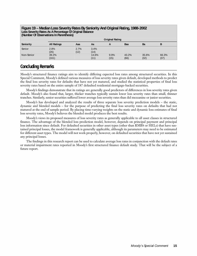
The median loss severity rates by seniority after controlling for the original rating are shown in Figure 19. As illus-trated, senior securities were rated either Aaa or Aa and sustained very low loss severity rates given default. In addition,within non-senior securities, the loss severity rate generally increases as the rating decreases. But there are two excep-tions. Defaulted securities rated Aa at origination had a higher median loss severity rates than did those rated A, andthose rated Baa at origination had a higher median loss severity rate than those rated Ba.

Figure 17 – Median Loss Severity Rates By Tranche Size And Original Rating, 1988-2002Loss Severity Rates As A Percentage Of Original Balance (Number Of Observations In Parenthesis)

Original Rating

Tranche Size at Origination All Ratings Aaa Aa A Baa Ba B

Greater than 70% 2.8% 2.7% 3.4% 1.0% 5.1%(29) (12) (14) (2) (1)

Between 10% and 70% 6.7% 5.7% 5.4% 14.1% 28.2% 3.7%(13) (4) (1) (2) (5) (1)

Between 5% and 10% 32.3% 14.8% 20.9% 43.2% 35.0% 27.5%(53) (7) (7) (34) (2) (3)

Between 2% and 5% 43.7% 9.9% 44.9% 41.2% 58.1%(43) (5) (23) (10) (5)

Less than 2% 53.0% 33.5% 37.9% 70.2%(49) (7) (14) (28)

All 32.3% 2.7% 6.3% 9.9% 43.2% 35.6% 66.3%(187) (12) (25) (15) (66) (32) (37)

Figure 18 – Median Loss Severity Rates By Seniority, 1988-2002

15%

59%

39%

3%

0%

10%

20%

30%

40%

50%

60%

70%

Senior Non-Senior

% of Original Balance

% of Default Date Balance


Concluding Remarks

Moody’s structured finance ratings aim to identify differing expected loss rates among structured securities. In thisSpecial Comment, Moody’s defined various measures of loss severity rates given default, developed methods to predictthe final loss severity rates for defaults that have not yet matured, and studied the statistical properties of final lossseverity rates based on the entire sample of 187 defaulted residential mortgage-backed securities.

Moody’s findings demonstrate that its ratings are generally good predictors of differences in loss severity rates givendefault. Moody’s also found that, larger, thicker tranches typically sustain lower loss severity rates than small, thinnertranches. Similarly, senior securities suffered lower average loss severity rates than did mezzanine or junior securities.

Moody’s has developed and analyzed the results of three separate loss severity prediction models – the static,dynamic and blended models – for the purpose of predicting the final loss severity rates on defaults that had notmatured at the end of sample period. By placing time-varying weights on the static and dynamic loss estimates of finalloss severity rates, Moody’s believes the blended model produces the best results.

Moody’s views its proposed measures of loss severity rates as generally applicable to all asset classes in structuredfinance. The advantage of the blended loss prediction model, however, depends on principal payment and principalloss information since default. For defaulted securities in other asset types (other than RMBS or HELs) that have sus-tained principal losses, the model framework is generally applicable, although its parameters may need to be estimatedfor different asset types. The model will not work properly, however, on defaulted securities that have not yet sustainedany principal losses.

The findings in this research report can be used to calculate average loss rates in conjunction with the default ratesor material impairment rates reported in Moody’s first structured finance default study. That will be the subject of afuture report.

Figure 19 – Median Loss Severity Rates By Seniority And Original Rating, 1988-2002Loss Severity Rates As A Percentage Of Original Balance (Number Of Observations In Parenthesis)

Original Rating

Seniority All Ratings Aaa Aa A Baa Ba B

Senior 2.8% 2.7% 3.4%(26) (12) (14)

Non-Senior 39.2% 14.6% 9.9% 43.2% 35.6% 66.3%(161) (11) (15) (66) (32) (37)


Appendix 1: Terminology

Payment DefaultA structured finance security is in payment default if it has suffered an interest shortfall or a principal write-down. Pre-payment interest shortfalls are not payment defaults.

Cured And Uncured Payment DefaultA payment default is cured as of a given date if there is no more loss outstanding on that date. A default is uncured ifthere are losses outstanding on that date. The cure status of a payment default is defined relative to a reference date,which is typically the end of a study period. This paper focuses on uncured payment defaults.

Material ImpairmentA structured security is in material impairment if it is an uncured payment default, or a Ca- or C-rated security that isnot yet in payment default.

Matured And Non-Matured DefaultsA defaulted security is matured if it has no remaining principal balance outstanding as of a given date. Otherwise, it iscalled non-matured.

Loss Severity Rate (LGD, Loss Given Default)The loss severity rate given default is the discounted present value of lifetime losses (both interest shortfalls and princi-pal losses included) as of a reference date – default date or origination date. One minus the loss severity rate is therecovery rate.

Default-Date Balance And Original BalanceDefault date balance is the outstanding principal balance at the time of default. Original balance is the principal bal-ance at the time of origination.

Tranche SizeTranche size is measured by the tranche principal balance at origination as a percentage of total deal balance at origina-tion.

Time To DefaultTime to default is the number of months from origination to default.

Static ModelThe static loss prediction model refers to a multi-factor regression model that uses only static factors – tranche size,time to default and default date balance – to predict final loss severity rates. These factors are static, in the sense thatthey do not change with the time since default.

Dynamic ModelThe dynamic loss prediction model refers to a single factor regression model that uses a dynamic factor – the ratio ofprincipal reduced to date due to loss versus total principal reduction since default date – and a parameter “beta” to pre-dict the future loss severity rate as a share of the remaining principal balance.

Blended ModelThe blended loss prediction model mixes the static and dynamic loss predictions using a weight variable “alpha” that istime varying after default. The blended model places a larger weight on the dynamic loss severity estimate for seasonedsecurities but a smaller weight on the dynamic loss severity estimate for newly defaulted securities.


Appendix 2: Illustrations Of Loss Severity Prediction Models

In Figure 20, we demonstrate the concepts of the dynamic loss severity prediction model presented in Figure 10.

As illustrated, a security was issued at time O with an original principal balance of PO. The curved line of O-G-H-J represents cumulative principal balance reduction, which is the sum of the amount of cumulative principal paid andthe amount of cumulative loss.

At time D, the security defaulted resulting in a loss to date of HI, or Lt. The cumulative amount of principal paidfrom D to t is represented by IM.

The line segment HM is the total principal balance reduced since default, which is BD – Bt. The right hand sidevariable in Figure 11, Lt/ (BD – Bt), is HI/HM.

The projected remaining loss RLt is represented by the line segment JK. Therefore, the left hand side variable inFigure 11, RLt/Bt, is represented by JK/JN, the projected remaining loss as a percentage of the remaining principalbalance. The dashed line IL, which is parallel to HK, is the projected actual principal payment line; that is, JL is thefinal loss amount (Lt + RLt). The lines HK and IL are assumed to be straight (the first-order approximation) as ourgoal is to estimate the final loss level, not the loss accumulation pattern.

In addition, Figure 20 assumes that the beta in Figure 11 is less than one. In other words, HI/HM, which is theindependent variable, is greater than JK/JN, the dependent variable. If beta is equal to one, the end point of the pro-jected final loss line would be much lower than point L (the end point of the dynamic loss estimate when beta is lessthan 1).

The maximum amount of loss (without discounting for illustrative purposes) is represented by JR, which is thesum of Lt and Bt .

Now let’s examine how the blended model weights the static loss estimate with the dynamic loss estimate (Figure21).

Figure 20 – The Dynamic Loss Severity Prediction Model – An Illustration

time

Cumulative Principal Payment / Cumulative Loss

PO

O(origination date)

D (default date)

t (current date)

T(maturity date)

Final Loss

Default Date Balance B D

Remaining Loss RL t

H

J

K

IG

L

Loss to Date L t

Remaining Principal Balance B t

N

M

Maximum Loss

R


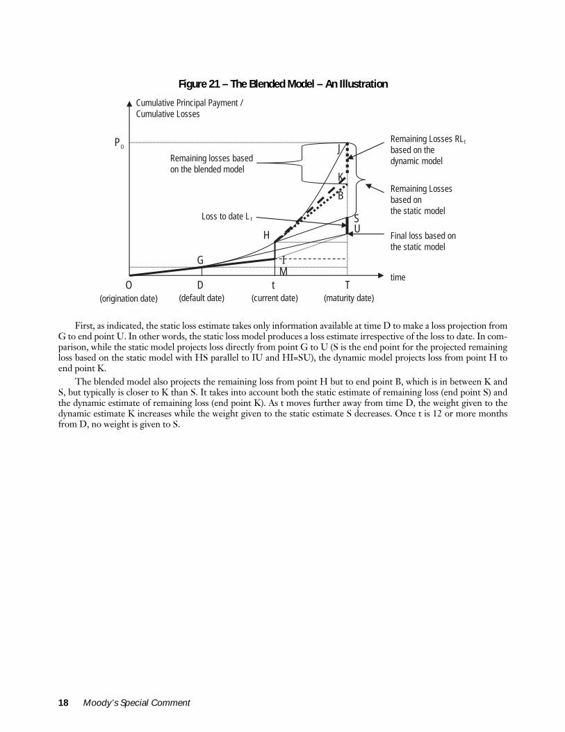
First, as indicated, the static loss estimate takes only information available at time D to make a loss projection fromG to end point U. In other words, the static loss model produces a loss estimate irrespective of the loss to date. In com-parison, while the static model projects loss directly from point G to U (S is the end point for the projected remainingloss based on the static model with HS parallel to IU and HI=SU), the dynamic model projects loss from point H toend point K.

The blended model also projects the remaining loss from point H but to end point B, which is in between K andS, but typically is closer to K than S. It takes into account both the static estimate of remaining loss (end point S) andthe dynamic estimate of remaining loss (end point K). As t moves further away from time D, the weight given to thedynamic estimate K increases while the weight given to the static estimate S decreases. Once t is 12 or more monthsfrom D, no weight is given to S.

Figure 21 – The Blended Model – An Illustration

Cumulative Principal Payment / Cumulative Losses

PO

O(origination date)

D (default date)

t (current date)

T (maturity date)

Remaining Losses RL based on the dynamic model

t

H

J

K

IGM time

Remaining Losses based on the static model

S

B

Remaining losses based on the blended model

Final loss based on the static model

ULoss to date L t


Appendix 3: List Of Defaults Included In This Study

Tranche Name Deal NameOriginal Rating

Asset Type

Default Year.Month

Matured as of 12/31/02

4A American Mtg Trust 1993-04 Ba2 RMBS 1996.09 YESB-3 C-BASS ABS, LLC Trust Certificates, Series 1998-2 B2 RMBS 2002.11 B Citicorp Mtg Sec Inc 1991-05 Baa2 RMBS 1994.09 B-1 Citicorp Mtg Sec Inc 1993-08 Baa3 RMBS 1996.01 B-1 Citicorp Mtg Sec Inc 1993-10 Baa3 RMBS 2002.01 A ComFed Savings Bank 1988-02 Aa2 RMBS 1992.04 A1 ComFed Savings Bank 1988-03 Aa2 RMBS 1992.05 YESA-1 ComFed Savings Bank 1988-06 Aa2 RMBS 1992.06 YESA-3 DLJ Mtg Acpt Corp 1992-Q07 Aa2 RMBS 1998.10 A-3 DLJ Mtg Acpt Corp 1992-Q08 Aa2 RMBS 1998.04 YESB-1 DLJ Mtg Acpt Corp 1992-Q08 Baa2 RMBS 1996.11 YESB-1 DLJ Mtg Acpt Corp 1993-Q03 Baa2 RMBS 1997.12 B-1 DLJ Mtg Acpt Corp 1993-Q06 Baa2 RMBS 1998.05 B-1 DLJ Mtg Acpt Corp 1993-Q13 Baa3 RMBS 1998.05 B-1 DLJ Mtg Acpt Corp 1993-Q16 Baa3 RMBS 1998.03 B-1 DLJ Mtg Acpt Corp 1993-QE01 Baa2 RMBS 1996.12 YESB-1 DLJ Mtg Acpt Corp 1993-QE05 Baa2 RMBS 1996.07 B-1 DLJ Mtg Acpt Corp 1993-QE11 Baa2 RMBS 1996.08 Cl. B-1 DLJ Mtg Acpt Corp 1994-Q12 Baa3 RMBS 2000.02 I B-2 DLJ Mtg Acpt Corp 1994-Q13 B3 RMBS 1997.10 YESII B-1 DLJ Mtg Acpt Corp 1994-Q13 Baa3 RMBS 1999.04 II B-2 DLJ Mtg Acpt Corp 1994-Q13 B3 RMBS 1997.09 YESIII B-1 DLJ Mtg Acpt Corp 1994-Q13 Baa3 RMBS 1997.05 III B-2 DLJ Mtg Acpt Corp 1994-Q13 B3 RMBS 1997.02 YESB-1 DLJ Mtg Acpt Corp 1994-Q14 Baa3 RMBS 1998.03 I B-1 DLJ Mtg Acpt Corp 1994-Q16 Baa3 RMBS 1998.05 II B-1 DLJ Mtg Acpt Corp 1994-Q16 Baa3 RMBS 1996.12 B-1 DLJ Mtg Acpt Corp 1994-QE01 Baa2 RMBS 1997.03 B-2 DLJ Mtg Acpt Corp 1994-QE01 B2 RMBS 1997.01 YESB-1 DLJ Mtg Acpt Corp 1994-QE02 Baa2 RMBS 1997.11 B-1 DLJ Mtg Acpt Corp 1994-QE04 Baa2 RMBS 1997.08 B-2 DLJ Mtg Acpt Corp 1994-QE04 B1 RMBS 1997.01 YESA-1 DLJ Mtg Acpt Corp 1994-QE05 Aaa RMBS 2000.04 YESA-2 DLJ Mtg Acpt Corp 1994-QE05 Aa1 RMBS 1999.04 YESB-1 DLJ Mtg Acpt Corp 1994-QE05 Baa2 RMBS 1997.03 YESB-2 DLJ Mtg Acpt Corp 1994-QE05 B1 RMBS 1996.10 YESA-1 DLJ Mtg Acpt Corp 1994-QE07 Aaa RMBS 1999.04 YESA-2 DLJ Mtg Acpt Corp 1994-QE07 Aa1 RMBS 1998.10 YESB-1 DLJ Mtg Acpt Corp 1994-QE07 Baa1 RMBS 1997.03 YESB-2 DLJ Mtg Acpt Corp 1994-QE07 Ba3 RMBS 1996.11 YESB-1 DLJ Mtg Acpt Corp 1995-Q01 Baa2 RMBS 1998.07 B-1 DLJ Mtg Acpt Corp 1995-Q02 Baa2 RMBS 1997.12 B-2 DLJ Mtg Acpt Corp 1995-Q02 B2 RMBS 1997.08 YESI B-1 DLJ Mtg Acpt Corp 1995-Q03 Baa3 RMBS 1998.10 II B-1 DLJ Mtg Acpt Corp 1995-Q03 Baa3 RMBS 1998.05 B-1 DLJ Mtg Acpt Corp 1995-Q05 Baa3 RMBS 1998.08 B-2 DLJ Mtg Acpt Corp 1995-Q05 B3 RMBS 1997.06 YESB-1 DLJ Mtg Acpt Corp 1995-Q06 Baa3 RMBS 1999.04 B-2 DLJ Mtg Acpt Corp 1995-Q06 B3 RMBS 1997.11 YESB-1 DLJ Mtg Acpt Corp 1995-Q08 Baa3 RMBS 1999.06 B-2 DLJ Mtg Acpt Corp 1995-Q08 B3 RMBS 1998.02 YESB-2 DLJ Mtg Acpt Corp 1995-Q10 Baa3 RMBS 1999.05 B-1 DLJ Mtg Acpt Corp 1995-Q11 Baa3 RMBS 1996.11 YESB-2 DLJ Mtg Acpt Corp 1995-Q11 B3 RMBS 1998.06 YESA-1 DLJ Mtg Acpt Corp 1995-QE01 Aaa RMBS 1999.03 YESA-2 DLJ Mtg Acpt Corp 1995-QE01 Aa2 RMBS 1998.08 YESB DLJ Mtg Acpt Corp 1995-QE01 Baa2 RMBS 1996.12 YESA-1 DLJ Mtg Acpt Corp 1995-QE03 Aaa RMBS 1999.07 A-2 DLJ Mtg Acpt Corp 1995-QE03 Aa1 RMBS 1998.11 YESB DLJ Mtg Acpt Corp 1995-QE03 Baa2 RMBS 1997.03 YESA-1 DLJ Mtg Acpt Corp 1995-QE08 Aaa RMBS 1999.09 A-2 DLJ Mtg Acpt Corp 1995-QE08 Aa2 RMBS 1999.03 YESB DLJ Mtg Acpt Corp 1995-QE08 Baa3 RMBS 1997.06 YESA-1 DLJ Mtg Acpt Corp 1995-QE09 Aaa RMBS 2000.01


A-2 DLJ Mtg Acpt Corp 1995-QE09 Aa2 RMBS 1999.08 YESB DLJ Mtg Acpt Corp 1995-QE09 Baa3 RMBS 1997.09 YESA-1 DLJ Mtg Acpt Corp 1995-QE11 Aaa RMBS 1999.06 YESA-2 DLJ Mtg Acpt Corp 1995-QE11 Aa2 RMBS 1999.02 YESB DLJ Mtg Acpt Corp 1995-QE11 Baa3 RMBS 1997.09 YESB DLJ Mtg Acpt Corp 1995-T07 Baa3 RMBS 1996.09 B-2 DLJ Mtg Acpt Corp 1996-Q1 Baa3 RMBS 2000.01 B-1 DLJ Mtg Acpt Corp 1996-Q2 A2 RMBS 2000.02 B-2 DLJ Mtg Acpt Corp 1996-Q2 Baa3 RMBS 1998.06 YESB-2 DLJ Mtg Acpt Corp 1996-Q4 A3 RMBS 1999.03 B-3 DLJ Mtg Acpt Corp 1996-Q4 Baa3 RMBS 1998.09 YESB-2 DLJ Mtg Acpt Corp 1996-Q5 Baa3 RMBS 1999.04 B-3 DLJ Mtg Acpt Corp 1996-Q5 Ba3 RMBS 1998.12 YESB-2 DLJ Mtg Acpt Corp 1996-Q6 Baa3 RMBS 1999.08 B-1 DLJ Mtg Acpt Corp 1996-QA Baa3 RMBS 1999.02 B-2 DLJ Mtg Acpt Corp 1996-QA B3 RMBS 1998.06 YESB-2 DLJ Mtg Acpt Corp 1996-QB Ba2 RMBS 1999.08 A-1 DLJ Mtg Acpt Corp 1996-QE3 Aaa RMBS 2000.03 A-2 DLJ Mtg Acpt Corp 1996-QE3 Aa2 RMBS 1999.09 YESB DLJ Mtg Acpt Corp 1996-QE3 A3 RMBS 1998.04 YESB-3 DLJ Mtg Acpt Corp 1996-QJ Ba3 RMBS 1999.04 Class A DLJ Mtg Acpt Corp 1997-A Aaa RMBS 2002.04 B-1 Fund America Investors Corp 1993-H Baa2 RMBS 2000.04 YESB-2 Fund America Investors Corp 1993-H B3 RMBS 1996.06 YESB Fund America Investors Corp II 1993-A Ba2 RMBS 1999.05 A-2 Greenwich Capital Acpt 1991-A Aa2 RMBS 1992.12 YESB-1 Greenwich Capital Acpt 1991-B Baa3 RMBS 1994.08 YESB-1 Greenwich Capital Acpt 1992-01 A3 RMBS 1998.01 YESB-2 Greenwich Capital Acpt 1992-01 Baa3 RMBS 1997.03 YESB-1 Greenwich Capital Acpt 1992-LB2 Baa3 RMBS 1996.02 YESB-1 Greenwich Capital Acpt 1992-LB5 Baa3 RMBS 1996.03 YESB-1 Greenwich Capital Acpt 1992-LB6 Baa3 RMBS 1996.06 YESB-1 Greenwich Capital Acpt 1992-LB8 Baa3 RMBS 1996.06 YESB-1 Greenwich Capital Acpt 1993-LB2 Baa3 RMBS 1997.05 YESB-1 Greenwich Capital Acpt 1994-LB3 Baa3 RMBS 1999.08 YESB-1 Greenwich Capital Acpt 1994-LB6 Baa3 RMBS 1999.11 YESB Greenwich Capital Acpt 1996-B Ba2 RMBS 2000.05 A Guardian S&L Assn 1989-11 Aa2 RMBS 1998.08 A Guardian S&L Assn 1989-12 Aa2 RMBS 1997.04 A Guardian S&L Assn 1990-01 Aa2 RMBS 1996.05 A Guardian S&L Assn 1990-03 Aa2 RMBS 1996.02 A Guardian S&L Assn 1990-04 Aa2 RMBS 1992.07 A1 Guardian S&L Assn 1990-05 Aa2 RMBS 1995.04 A-1 Guardian S&L Assn 1990-06 Aaa RMBS 1998.07 A Guardian S&L Assn 1990-07 Aa2 RMBS 1995.02 A-1 Guardian S&L Assn 1990-08 Aaa RMBS 1997.01 A-1 Guardian S&L Assn 1991-01 Aaa RMBS 1995.07 M Housing Securities Inc 1992-9 A2 RMBS 1994.06 YESC3 Imperial CMB Trust 1998-1 B3 RMBS 1999.05 IIB-1 MDC Mtg Funding Corp (Greenwich/Long Beach) 1994-LB7 Baa3 RMBS 1999.06 YESC Morgan Stanley Capital I Inc. Series 1997-P2 B3 RMBS 2001.05 YESA Nomura Asset Capital Corp 1994-01 Aa2 RMBS 1997.10 A-1 PaineWebber Mtg Acpt IV 1991-01 (Coast) Aa2 RMBS 1992.05 YESB-4 Pass-Through Asset Class Execution 1997-I (CWMBS 1997-4) B2 RMBS 2001.08 A Prudential Home Mtg Co 1988-05 Aa2 RMBS 1992.08 B3-1 Prudential Home Mtg Co 1992-A A2 RMBS 1997.10 B3-2 Prudential Home Mtg Co 1992-A A2 RMBS 1997.10 B3-3 Prudential Home Mtg Co 1992-A A2 RMBS 1997.10 B3-4 Prudential Home Mtg Co 1992-A A2 RMBS 1997.10 B4 Prudential Home Mtg Co 1992-A Baa2 RMBS 1995.12 YESB5 Prudential Home Mtg Co 1992-B Ba3 RMBS 1993.06 B-3 Prudential Home Mtg Co 1993-17 Ba2 RMBS 1999.06 YESB-2 Prudential Home Mtg Co 1993-24 Ba2 RMBS 1999.02 YESB3 Prudential Home Mtg Co 1993-F Ba2 RMBS 1997.12 YESB6 Prudential Home Mtg Co 1995-C B3 RMBS 1998.01 YESA RFC Mtg Exchange Corp 1989-SW-1B Aa2 RMBS 1992.02 C-2 Ryland Mtg Sec 1993-06B Baa3 RMBS 2001.06


Asset Type

Default Year.Month



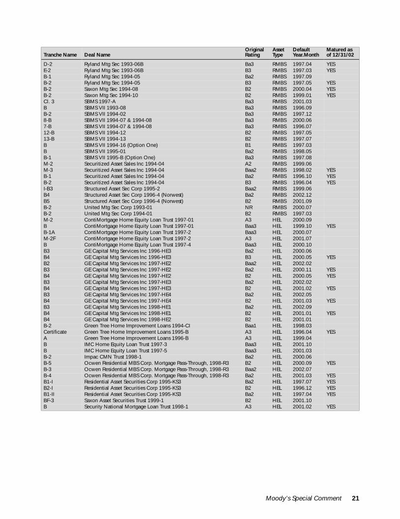
D-2 Ryland Mtg Sec 1993-06B Ba3 RMBS 1997.04 YESE-2 Ryland Mtg Sec 1993-06B B3 RMBS 1997.03 YESB-1 Ryland Mtg Sec 1994-05 Ba2 RMBS 1997.09 B-2 Ryland Mtg Sec 1994-05 B3 RMBS 1997.05 YESB-2 Saxon Mtg Sec 1994-08 B2 RMBS 2000.04 YESB-2 Saxon Mtg Sec 1994-10 B2 RMBS 1999.01 YESCl. 3 SBMS 1997-A Ba3 RMBS 2001.03 B SBMS VII 1993-08 Ba3 RMBS 1996.09 B-2 SBMS VII 1994-02 Ba3 RMBS 1997.12 8-B SBMS VII 1994-07 & 1994-08 Ba3 RMBS 2000.06 7-B SBMS VII 1994-07 & 1994-08 Ba3 RMBS 1996.07 12-B SBMS VII 1994-12 B2 RMBS 1997.05 13-B SBMS VII 1994-13 B2 RMBS 1997.07 B SBMS VII 1994-16 (Option One) B1 RMBS 1997.03 B SBMS VII 1995-01 Ba2 RMBS 1998.05 B-1 SBMS VII 1995-B (Option One) Ba3 RMBS 1997.08 M-2 Securitized Asset Sales Inc 1994-04 A2 RMBS 1999.06 M-3 Securitized Asset Sales Inc 1994-04 Baa2 RMBS 1998.02 YESB-1 Securitized Asset Sales Inc 1994-04 Ba2 RMBS 1996.10 YESB-2 Securitized Asset Sales Inc 1994-04 B3 RMBS 1996.04 YESI-B3 Structured Asset Sec Corp 1995-2 Baa2 RMBS 1999.06 B4 Structured Asset Sec Corp 1996-4 (Norwest) Ba2 RMBS 2002.12 B5 Structured Asset Sec Corp 1996-4 (Norwest) B2 RMBS 2001.09 B-2 United Mtg Sec Corp 1993-01 NR RMBS 2000.07 B-2 United Mtg Sec Corp 1994-01 B2 RMBS 1997.03 M-2 ContiMortgage Home Equity Loan Trust 1997-01 A3 HEL 2000.09 B ContiMortgage Home Equity Loan Trust 1997-01 Baa3 HEL 1999.10 YESB-1A ContiMortgage Home Equity Loan Trust 1997-2 Baa3 HEL 2000.07 M-2F ContiMortgage Home Equity Loan Trust 1997-2 A3 HEL 2001.07 B ContiMortgage Home Equity Loan Trust 1997-4 Baa3 HEL 2000.10 B3 GE Capital Mtg Services Inc 1996-HE3 Ba2 HEL 2000.06 B4 GE Capital Mtg Services Inc 1996-HE3 B3 HEL 2000.05 YESB2 GE Capital Mtg Services Inc 1997-HE2 Baa2 HEL 2002.02 B3 GE Capital Mtg Services Inc 1997-HE2 Ba2 HEL 2000.11 YESB4 GE Capital Mtg Services Inc 1997-HE2 B2 HEL 2000.05 YESB3 GE Capital Mtg Services Inc 1997-HE3 Ba2 HEL 2002.02 B4 GE Capital Mtg Services Inc 1997-HE3 B2 HEL 2001.02 YESB3 GE Capital Mtg Services Inc 1997-HE4 Ba2 HEL 2002.05 B4 GE Capital Mtg Services Inc 1997-HE4 B2 HEL 2001.03 YESB3 GE Capital Mtg Services Inc 1998-HE1 Ba2 HEL 2002.09 B4 GE Capital Mtg Services Inc 1998-HE1 B2 HEL 2001.01 YESB4 GE Capital Mtg Services Inc 1998-HE2 B2 HEL 2001.01 B-2 Green Tree Home Improvement Loans 1994-CI Baa1 HEL 1998.03 Certificate Green Tree Home Improvement Loans 1995-B A3 HEL 1996.04 YESA Green Tree Home Improvement Loans 1996-B A3 HEL 1999.04 B IMC Home Equity Loan Trust 1997-3 Baa3 HEL 2001.10 B IMC Home Equity Loan Trust 1997-5 Baa3 HEL 2001.03 B-2 Impac CMN Trust 1998-1 Ba2 HEL 2000.06 B-5 Ocwen Residential MBS Corp. Mortgage Pass-Through, 1998-R3 B2 HEL 2000.09 YESB-3 Ocwen Residential MBS Corp. Mortgage Pass-Through, 1998-R3 Baa2 HEL 2002.07 B-4 Ocwen Residential MBS Corp. Mortgage Pass-Through, 1998-R3 Ba2 HEL 2001.03 YESB1-I Residential Asset Securities Corp 1995-KS3 Ba2 HEL 1997.07 YESB2-I Residential Asset Securities Corp 1995-KS3 B2 HEL 1996.12 YESB1-II Residential Asset Securities Corp 1995-KS3 Ba2 HEL 1997.04 YESBF-3 Saxon Asset Securities Trust 1999-1 B2 HEL 2001.10 B Security National Mortgage Loan Trust 1998-1 A3 HEL 2001.02 YES


Asset Type

Default Year.Month



Related Research

Rating Methodology:Moody's Approach To Rating Synthetic Resecuritizations, October 2003, #SF27650Special Comment:Default & Recovery Rates of Corporate Bond Issuers 1920-2003, January 2004, #80989Payment Defaults And Material Impairments Of U.S. Structured Finance Securities: 1993-2002, December 2003,#80247Recovery Rates on Defaulted Corporate Bonds and Preferred Stocks, 1982-2003, December 2003, #80272Structured Finance Rating Transitions: 1983-2003, February 2004, #81239Structured Finance Rating Transitions: 1983-2002, January 2003, #77291Special Report:Moody's Approach to Rating Multisector CDOs, September 15, 2000, #SF9050

To access any of these reports, click on the entry above. Note that these references are current as of the date of publication of thisreport and that more recent reports may be available. All research may not be available to all clients.


http://www.moodys.com/moodys/cust/research/venus/Publication/Special%20Comment/noncategorized_number/81239.pdf




http://www.moodys.com/moodys/cust/research/avalon/Publication/Rating%20Methodology/noncategorized_number/SF9050.pdf

http://www.moodys.com/moodys/cust/research/avalon/Publication/Rating%20Methodology/noncategorized_number/SF27650.pdf


PAGE INTENTIONALLY LEFT BLANK

© Copyright 2004, Moody’s Investors Service, Inc. and/or its licensors including Moody’s Assurance Company, Inc. (together, “MOODY’S”). All rights reserved. ALL INFORMATIONCONTAINED HEREIN IS PROTECTED BY COPYRIGHT LAW AND NONE OF SUCH INFORMATION MAY BE COPIED OR OTHERWISE REPRODUCED, REPACKAGED, FURTHERTRANSMITTED, TRANSFERRED, DISSEMINATED, REDISTRIBUTED OR RESOLD, OR STORED FOR SUBSEQUENT USE FOR ANY SUCH PURPOSE, IN WHOLE OR IN PART, IN ANYFORM OR MANNER OR BY ANY MEANS WHATSOEVER, BY ANY PERSON WITHOUT MOODY’S PRIOR WRITTEN CONSENT. All information contained herein is obtained byMOODY’S from sources believed by it to be accurate and reliable. Because of the possibility of human or mechanical error as well as other factors, however, such information is provided “asis” without warranty of any kind and MOODY’S, in particular, makes no representation or warranty, express or implied, as to the accuracy, timeliness, completeness, merchantability or fitnessfor any particular purpose of any such information. Under no circumstances shall MOODY’S have any liability to any person or entity for (a) any loss or damage in whole or in part caused by,resulting from, or relating to, any error (negligent or otherwise) or other circumstance or contingency within or outside the control of MOODY’S or any of its directors, officers, employees oragents in connection with the procurement, collection, compilation, analysis, interpretation, communication, publication or delivery of any such information, or (b) any direct, indirect,special, consequential, compensatory or incidental damages whatsoever (including without limitation, lost profits), even if MOODY’S is advised in advance of the possibility of suchdamages, resulting from the use of or inability to use, any such information. The credit ratings and financial reporting analysis observations, if any, constituting part of the informationcontained herein are, and must be construed solely as, statements of opinion and not statements of fact or recommendations to purchase, sell or hold any securities. NO WARRANTY,EXPRESS OR IMPLIED, AS TO THE ACCURACY, TIMELINESS, COMPLETENESS, MERCHANTABILITY OR FITNESS FOR ANY PARTICULAR PURPOSE OF ANY SUCH RATING OR OTHEROPINION OR INFORMATION IS GIVEN OR MADE BY MOODY’S IN ANY FORM OR MANNER WHATSOEVER. Each rating or other opinion must be weighed solely as one factor in anyinvestment decision made by or on behalf of any user of the information contained herein, and each such user must accordingly make its own study and evaluation of each security and ofeach issuer and guarantor of, and each provider of credit support for, each security that it may consider purchasing, holding or selling. MOODY’S hereby discloses that most issuers of debtsecurities (including corporate and municipal bonds, debentures, notes and commercial paper) and preferred stock rated by MOODY’S have, prior to assignment of any rating, agreed to payto MOODY’S for appraisal and rating services rendered by it fees ranging from $1,500 to $1,800,000.


To order reprints of this report (100 copies minimum), please call 1.212.553.1658.Report Number: 86769

Authors Editor Associate Analyst Production Specialist

Jian Hu Michael D’Arcy Alexandra Neely John TzanosRichard Cantor

Measuring Loss Severity Rates Of Defaulted Residential ... · PDF fileSpecial Comment...

Documents

Transcript of Measuring Loss Severity Rates Of Defaulted Residential ... · PDF fileSpecial Comment...