
Census 2000 PHC-T-4. Ranking Tables for Counties: 1990 and 2000
Demographic Research a free, expedited, online journal of peer-reviewed research and commentary in the population sciences published by the Max Planck Institute for Demographic Research Doberaner Strasse 114 · D-18057 Rostock · GERMANY www.demographic-research.org
DEMOGRAPHIC RESEARCH VOLUME 3, ARTICLE 10 PUBLISHED 7 NOVEMBER 2000 www.demographic-research.org/Volumes/Vol3/10/ DOI: 10.4054/DemRes.2000.3.10
Measuring Local Heterogeneity with 1990 U.S. Census Data
Kenneth W. Wachter
David A. Freedman
© 2000 Max-Planck-Gesellschaft.

Demographic Research - Volume 3, Article 10
Measuring Local Heterogeneity with 1990 U.S. Census Data
Kenneth W. Wachter1
David A. Freedman2
AbstractA sample covering 204,394 blocks from the 1990 U.S. Census permits measurement of residual
heterogeneity from local area to local area after controlling by strati¿cation for demographic char-
acteristics such as race, ethnicity, age, sex as well as geographic characteristics such as region and
place-type. The local areas have populations on the order of 10,000 people. The variables studied
are four indices of enumeration dif¿culty. The results show that variance due to heterogeneity
from area to area is comparable to (if not larger than) variance from stratum to stratum and can be
expected to dominate sampling variance - especially with samples as large as the ones used in the
U.S. Census Bureau’s Post-Enumeration Surveys. These¿ndings constrain the viable estimation
strategies that could be employed for local tallies in the U.S. 2000 Census.
1Professor of Demography and of Statistics, University of California, Berkeley, CA 947202Professor of Statistics, University of California, Berkeley, CA 94720
http://demographic-research.org/Volumes/Vol3/10/ 7 November 2000
Demographic Research - Volume 3, Article 10
1 Introduction
In the United States, census counts are used to apportion congressional seats to states, and to
draw the boundaries of electoral districts within states (“redistricting”). The counts also enter the
formulas for allocating tax funds to states, counties, cities, and smaller jurisdictions. Thus, the
census has some effect on the distribution of power and money [Skerry 2000]. Controversy over
proposed statistical adjustments of population counts from decennial censuses has stimulated an
extended program of demographic research over twenty years [see 4]. These issues have been
brought again to the fore by the current Director of the U.S. Census Bureau, Kenneth Prewitt.
In considering whether to certify adjusted or unadjusted counts as the of¿cial census counts,
Prewitt directs attention to the problem of geographical heterogeneity in quality of coverage, which
limits the accuracy of small-area estimates� he acknowledges the renewed importance of data from
1990, recognizing that decisions will be made before much of the data from the 2000 Census
evaluation process will become available: he favors certifying the adjusted counts, barring some
unforeseen developments when the data are collected and analyzed [Prewitt 2000]. Because the
U.S. Supreme Court ruled that federal law mandates the use of unadjusted population counts for
apportionment, the impact of certi¿cation will be on the use of census data for redistricting within
states, and the allocation of tax funds to state and substate jurisdictions [Brown et al. 1999].
A large data set for studying geographical heterogeneity in quality of coverage for substate
areas as well as for states was assembled around 1990 by the U.S. Census Bureau in its P-12
Evaluation Project. However, most analysis was directed toward state-by-state heterogeneity. In
this paper, we analyze the scale of substate heterogeneity as revealed by the P-12 data, to provide
scienti¿c background for the political decisions at stake in the Prewitt report.
The issue of heterogeneity should be viewed in the broader statistical context of small-area
estimation. Classical statistical sampling theory is about inferences upward from the part to the
whole, from sample to population. Accuracy is limited by the size of the sample, essentially
through the square root of the sample size. In small-area estimation, the situation is different.
The aim is to make inferences sideways from a few parts to all other parts. The plan for the
U.S. Census in 2000 calls for extrapolating sideways from a sample of 12,000 block clusters to
separate estimates of census undercount for tens of thousands of local areas and each of 5 million
inhabited Census blocks. Accuracy is limited not only by sample size but also fundamentally by
the amount of heterogeneity from local area to local area. The square root law ceases to apply -
even if all data-processing can be done without error.
It is standard practice to apply uniform ratio estimators and other small-area techniques only
http://demographic-research.org/Volumes/Vol3/10/ 7 November 2000

Demographic Research - Volume 3, Article 10
after stratifying on available variables like age, sex, and race [Ghosh and Rao 1994]. Through
strati¿cation some heterogeneity is removed, leaving residual heterogeneity which at some point
still imposes diminishing returns on the gains in accuracy achievable from larger sample size.
Before 1990, little was known about levels of residual heterogeneity and the pace of diminishing
returns to sample size. Since then, interest in census adjustment has led to a series of studies in
the United States [see 4], principally focussed on state-to-state heterogeneity in various indices of
enumeration dif¿culty. The U.S. Census Bureau created, in its P-12 Evaluation Project, a unique
data set suitable for studying local as well as state-level heterogeneity. The present study exploits
P-12 to derive the¿rst - albeit somewhat tentative - measurements of residual heterogeneity for
local areas containing on the order of 10,000 people each.
The measurements of heterogeneity in this study provide a benchmark for assessing small-
area undercount estimation in the census. The issues are summarized in [Prewitt 2000], with
extensive references� for another perspective, see [Brown et al. 1999]. An underlying probability
model is useful for distinguishing the effects of geographical heterogeneity treated here from other
components of error [Freedman, Stark and Wachter 2000]. As well as playing a role in discussions
of Census adjustment, the measurements in the present study also bear on the likely accuracy of
small-area estimation in many other applications. They follow, in an American context, on the new
scienti¿c interest in structural properties of geographical heterogeneity kindled by [Le Bras 1993].
Several questions are frequently asked about research in this area. (i) Why study indices of
enumeration dif¿culty rather than undercounts themselves? (ii) Can residual heterogeneity not be
eliminated by¿ner strati¿cation? (iii) What about other datasets?
(i) The Census does not measure its own undercount. Surveys that do measure undercounts, large
as they are, are much too small to measure heterogeneity at any¿ne geographical scale. Problems
with data quality in the 1990 Post-Enumeration Survey (PES) also restrict its usefulness for ap-
praising heterogeneity. Data from the 2000 PES, renamed “Accuracy and Coverage Evaluation”
(ACE), will not be available for some time, and research projects to assess the data quality in ACE
have uncertain completion dates.
(ii) Possibilities for¿ner strati¿cation are limited. For Census Bureau purposes, only variables
recorded for all respondents on Census short forms are usable for strati¿cation. Moreover, there
is little evidence to show that doubling or tripling the number of post-strata would achieve any
marked reduction in heterogeneity� we return to this point, below.
(iii) Other publicly available data sets known to us lack one or another key feature of P-12. The
U.S. Public Use Microdata Samples (PUMS) only identify geographical location down to “Pub-
lic Use Microdata Areas” (PUMAs) with more than 100,000 people each. The Census Bureau’s
http://demographic-research.org/Volumes/Vol3/10/ 7 November 2000
Demographic Research - Volume 3, Article 10
Summary Tabulation Files have precise geography but little cross-classi¿cation by stratifying vari-
ables. The other large U.S. surveys, like the Current Population Survey, are much smaller than
P-12. Similar limitations of one kind or another apply to data sets collected in other developed
countries. The data for Frenchcommunes achieve geographical resolution an order of magnitude
¿ner than P-12, but lack strati¿cation variables [Le Bras 1993].
Every silver lining has its cloud, and P-12 is no exception. The P-12 data were aggregated by
the Bureau in a data-dependent way into “superblocks,” in order to protect the con¿dentiality of
the respondents. Superblocks range in size from a city block in Manhattan to some large swath
of rural Wyoming. The data we have are based on superblocks: our summary statistics show the
heterogeneity in these units, thereby averaging across a full spectrum of more familiar geography.
The data suggest, however, that a typical superblock represents a locality whose order of size is
10,000 inhabitants, and our results are best interpreted on that geographic scale. More formal
arguments are postponed to the Appendix.
http://demographic-research.org/Volumes/Vol3/10/ 7 November 2000

Demographic Research - Volume 3, Article 10
2 Heterogeneity
2.1 The Measure M
This section presents our measure of heterogeneity, and procedures for estimating it from the data.
Throughout this discussion we restrict attention to a single variable (e.g., the proportion of persons
living in multi-unit housing) and to a single demographic group, for example, Hispanic women
aged 20-29. Our object of study is variability from local area to local area within broader areas.
We need some terminology and notation to clarify the distinctions.
Territory is our name for one of the broader areas, and each territory spans many local ar-
eas. The territories are determined by the design of the underlying estimation project and data-
collection effort. In small-area estimation with uniform ratio estimators, all small areas within
one territory are assigned a common “uniform” estimated value, based on aggregating across the
territory� in census applications, estimates are uniform within combinations of territory and de-
mography called “post-strata.” Typically, a territory consists of all places of a particular type
across some regional subdivision of the country. In P-12, the central cities in New England are an
example of a territory.
Each territory is dissected intolocalities: examples might be the Back Bay, North End, or
Beacon Hill in Boston� or Colorado’s Snowmass Mountain Basin, Sangre de Cristos foothills,
etc. The estimation project itself may go down to smaller units than these local areas - Census
undercount estimation goes all the way down to blocks - but we are measuring heterogeneity only
down to the scale allowed by P-12. For any particular variable of interest, each local area has
a value that differs from the territory-wide value, the latter being an average of the former. The
deviations from average are what we call heterogeneity, and it is heterogeneity that we are going
to measure.
In our notation, within a given territory, for a given variable and demographic group:
R� is the true rate for all?� group members in the�th ofu localities�
R 'S
�R�*u is the arithmetic mean of the true local rates.
The quantity whose measurement is the goal of the study is the population-level “variance due to
heterogeneity,” the variance of the true local rates about their mean:
M2 '�
u
[�
ER� � R�2� i�j
This quantity is important because it appears in formulas for estimation error. Let�R be an estimator
http://demographic-research.org/Volumes/Vol3/10/ 7 November 2000

Demographic Research - Volume 3, Article 10
of R. The mean squared error of estimation that results from using �R as the estimate of R� for all
local areas as if they shared a common value is
�
u
[�
ER� � �R�2 ' M2 n ER� �R�2� i2j
The ¿rst term on the right, M2, represents errors due to heterogeneity resulting directly from at-
tributing one common rate to local areas whose true rates vary. The second term represents errors
due to bias and sampling variability in the territory-wide estimator�R. TheM2-term only van-
ishes if the local areas are in fact homogeneous, so that allR� equal each other and hence equalR.
Otherwise,M2 is a contribution to error which cannot be reduced by increasing sample size.
Some¿ne points require mention. To begin with,M2 is centered onR, in order to make straight-
forward the interpretation as a variance due to heterogeneity. Similarly,R is the unweighted mean
of theR�. The P-12 data were aggregated by a procedure that tends to equalize the counts of stratum
members in local areas, so there is little numerical difference between weighted and unweighted
means. Conceptually, however, the weighted mean is the natural target of a ratio estimator obtained
from a numerator and denominator separately aggregated over�. If �R is such an estimator, then the
term ER � �R�2 in i2j includes the squared difference between weighted and unweighted means,
as well as a contribution from sampling error and from “ratio estimator bias,” whose underlying
source is again heterogeneity among theR�. Ratio estimator bias enters throughR � �R, decreases
with sample size, and is a minor part of the story compared toM2 [Freedman, Stark and Wachter
2000].
We now discuss estimation ofM2 from the P-12 sample. Temporarily, we have¿xed a territory
and a variable, and are considering only persons in one demographic group. In our setup, the�th
superblock represents the�th locality, so the number of superblocks coincides with the number of
localities. Let
R� be the rate for the�� sample persons in the�th superblock�
R 'S
�R�*u be the mean of these rates.
A naive estimator ofM2 would be�
u
[�
ER� � R�2� i�j
However, this estimator of variance due to heterogeneity is inÀated by variance due to sampling.
http://demographic-research.org/Volumes/Vol3/10/ 7 November 2000

Demographic Research - Volume 3, Article 10
We therefore de¿ne M by the equation
M2 '�
u
[�
ER� � R�2 � �
u
��� �
u
�[�
R�E�� R��
�� � �� iej
The second term is an approximate correction for sampling variability in R� and R [see Appendix].
2.2 Variables and Strata
Four variables are examined in our study:
(i) The multi-unit housing rateis the proportion of persons residing in multi-unit structures.
(ii) The non-mailback rateis the proportion of people who did not mail back their Census form,
out of all people in the Census who were meant to mail it back.
(iii) The allocation rateis the proportion of persons with at least one of six key characteristics
imputed. The six characteristics are relationship to householder, age, sex, race, Hispanic origin,
and marital status.
(iv) The substitution rateis the proportion of persons whose whole record was imputed or “substi-
tuted” into the Census, typically in households from which no detailed information was obtained.
These variables provide a good variety of cases with which to examine local heterogeneity.
They include one structural variable, one behavioral variable, and two measures of data complete-
ness, all taking values between zero and one. They are four of the¿ve main variables treated in
the Census Bureau’s P-12 Project Report [Kim 1991]: the¿fth variable, the mail universe rate, is
more narrowly administrative in character, and is not considered here.
Documentation of the P-12 data set is to be found in [Thompson 1990, U.S. Bureau of the
Census 1990, Bateman 1991, Kim 1991]. The sample is a strati¿ed cluster sample selected using
essentially the same design as the Census Bureau’s 1990 Post-Enumeration Survey (PES) but with
116,619 block clusters in place of 5293. These clusters include 204,394 blocks compared to 12,964
blocks for the PES.
The strati¿cation is the one proposed for adjusting the 1990 Census. The population is divided
into 116 PSGs (“Post-Stratum Groups”) de¿ned in part by geography and in part by demography.
The geographical classi¿cation is based on census division (9 areas) and place-type (7 types). The
demographic breakdown is by race-ethnicity (4 categories), and renter-owner status (2 groups). In
principle, there could beb� .� e� 2 ' Dfe PSGs, but smaller ones are collapsed and the largest
urban areas are treated differently. In total, there are 116 PSGs: a list can be found in Table A.1 of
Hogan (1993). We exclude the PSG for Indians living on reservations, and deal with the remaining
http://demographic-research.org/Volumes/Vol3/10/ 7 November 2000

Demographic Research - Volume 3, Article 10
115� we also exclude the so-called “residual population” not surveyed by the PES. Each PSG is
broken down by 6 age groups and 2 sexes into 12 “post-strata,” so we have��D � �2 ' ��Hf
post-strata to consider.
Each post-stratum is de¿ned in part by demography (race-ethnicity, renter-owner, age, sex)
and in part by geography (census division, place-type). Three examples give theÀavor of the
post-strata:
(i) Non-minority females age 0-9 living in a central city in New England.
(ii) Black males age 10-19 living in rental units in a central city in a large metropolitan area in the
South Atlantic division (Florida, Georgia, and so forth).
(iii) Black and hispanic females age 60 and over in New England, living either in a central city or
in a metropolitan area but not in its central city
The geography is the “territory” associated with the post-stratum, and the demography can
be considered as providing the strati¿cation within which small-area estimation takes place. In
post-stratum (i), for instance, the territory is central cities in New England� small-area estimation
would be uniform within the part of this territory inhabited by the demographic group consisting of
non-minority females age 0-9. With post-stratum (ii), the territory consists of central cities in large
metropolitan areas in the South Atlantic division, and the demographic group consists of black
males age 10-19 living in rental units. Thus, the boundaries of the territories depend on the post-
stratum, and so will the dissection of each territory into local areas. For groups whose members
are numerous, high resolution is possible and the local areas are small. For groups whose members
are few and far between, the local areas are extended.
As noted above, the speci¿cation of territories, and localities within a territory, is data-dependent.
More speci¿cally, the records in P-12 correspond to unique - and non-overlapping - intersections
of post-strata and superblocks. These records were built up from more basic information for each
post-stratum and sample block. The algorithm used to build up the records required that for any
given post-stratum, a P-12 record must have at least ten post-stratum members� the corresponding
geography must span whole Census block clusters and must not cross state lines. (These three con-
straints could not always be satis¿ed, and we eliminated some 2000 exceptional records.) Given a
post-stratum, a “superblock” is the collection of block clusters put together during the construction
of a record� there is one superblock per record. There is one locality per superblock, consisting of
all the block clusters in the population corresponding to the one block cluster in the sample. Due
to the sample design, this informal idea can be made fairly precise [see Appendix].
The total U.S. population is around 250 million. Our P-12 dataset has about 12,000,000 people,
and we think of it as a 1-in-20 sample� in reality, the sampling fraction varies from one part of
http://demographic-research.org/Volumes/Vol3/10/ 7 November 2000
Demographic Research - Volume 3, Article 10
the country to another. There were 750,000 records, so the average number of sample persons
in a record is 12,000,000/750,000 ' 16: given a typical post-stratum and superblock, about 16
members of the post-stratum will be found in the superblock. This corresponds to roughly 300
post-stratum members per locality, since each sample person represents some 20 people. The
algorithm used to construct the P-12 records tends to equalize the local-area counts.
There are 115 PSGs� these do not overlap, and their average size is around 250 million/115
or 2.2 million people. Each PSG is de¿ned by a combination of geography - the “territory” - and
demography. The territories will have a population that is several times larger than the PSG: 5-10
million people is a representative range, so there must be several hundred localities per territory.
We estimate an average of 6 blocks per superblock, hence, 120 blocks per locality, with 6,000
persons in all demographic groups combined - although this is only an order-of-magnitude calcu-
lation. We have done the P-12 aggregation ourselves on the “Berkeley subset” of census data [see
Appendix], and those simulations suggest a population of 10,000 per locality. In the end, we think
most localities will have populations in the range 2,500-25,000.
The geometry is confusing at¿rst. The superblocks and localities associated with any particular
post-stratum do not overlap. As we move from one post-stratum to another within the same PSG,
the territory remains the same - but due to the aggregation procedure, the superblocks change and
new superblocks overlap the old. (Similar statements apply to the localities.) As we move from
one PSG to another, the territories change and overlap: compare post-strata (i) and (iii) above.
Although details are complicated, the basic picture is straightforward. There are two scales
which govern any measurement of heterogeneity. Variability occurs within some big unit, across
some small units. Here the big unit is a territory encompassing something like 7 million people.
The small units are local areas encompassing some 10,000 people, with about 300 people in each
of 30 demographic groups. On these scales, P-12 allows estimates of residual heterogeneity after
strati¿cation by demographic group. The measurement of heterogeneity within post-strata across
the superblocks of P-12 is relatively unambiguous� tying the results to more familiar geographical
units must be more tentative, due to the complexities of the P-12 data structure.
2.3 Results
Estimates of residual heterogeneity from P-12 are shown in Table 1, along with related values for
comparison. The four columns correspond to the four outcome variables in our study. The values
shown for M and for sampling standard error are root-mean-square (RMS) values calculated over
all post-strata. We reportM rather thanM2 to make units and scale more easily understandable.
http://demographic-research.org/Volumes/Vol3/10/ 7 November 2000

Demographic Research - Volume 3, Article 10
Table 1: Measures of Heterogeneity and Comparative Values
Multi-unit Non- Alloca- Substi-
housing mailback tions tutions
Measures of Heterogeneity
M for local areas 22.3% 10.7% 7.1% 2.3%
Standard error 0.7% 0.3% 0.2% 0.2%
M for states 10.4% 4.3% 2.9% 0.6%
Values for Comparison
Standard deviation of
R across post-strata 23.7% 12.0% 8.0% 0.7%
Mean ofR across post-strata 28.6% 29.7% 19.7% 1.1%
Sampling standard errors ofR
Low estimate 2.6% 3.0% 2.7% 0.7%
High estimate 6.1% 4.2% 3.4% 1.0%
The¿rst row of Table 1 showsMs for local areas in P-12. The¿rst entry is 22.3%, signifying
that within post-strata, the local area-to-area differences in the rates of multi-unit housing are on the
order of 22.3%. In other words, ascribing the overall rate of multi-unit housing to the local areas
within a territory incurs an RMS error due to heterogeneity of 22.3%, even after controlling for the
geographic and demographic variables in the post-strati¿cation. This outcome reveals a remarkable
degree of diversity in the clustering of apartment buildings and multiple-family houses. The other
entries range from 10.7% for the non-mailback rate down to 2.3% for the Census substitution rate.
The calculation of the standard errors is described below [see Appendix]� these are plausible upper
bounds.
If people belonging to the same post-stratum shared the same rates, wherever they resided, the
values ofM2 would all be estimates of zero. ThoughM2 is estimating a non-negative quantity, its
sample values are not constrained to be non-negative. None of the 1380 post-strata have negative
estimates for multi-unit housing or non-mailbacks� ¿ve do for allocations and 50 for substitutions.
The small standard errors and the rarity of negatives both indicate the strong statistical signi¿cance
of the observed heterogeneity, thanks to the large sample size of P-12.
Our formula for M can be applied to measure state-to-state heterogeneity by letting� in the
http://demographic-research.org/Volumes/Vol3/10/ 7 November 2000

Demographic Research - Volume 3, Article 10
de¿nition range over the 50 states plus the District of Columbia. The third row of Table 1 shows
the state-level RMS values ofM across the 1224 post-strata that intersect more than one state. We
see thatM for multi-unit housing only falls to a little less than half its local-level value at this much
larger level of aggregation. For substitutions,M is still one-fourth of its local level. Heterogeneity
is not simply produced by small-scaleÀutters in concentrations: if it were, heterogeneity would
average out at larger scales like states. The values for states in Table 1 are generally only a bit
smaller than the comparable values for states in Table 5 of [Freedman and Wachter 1994], where
a coarser 357-fold post-strati¿cation is used� the value for multi-unit housing is actually bigger.
This suggests that the measures of heterogeneity are somewhat robust to moderate changes in the
post-strati¿cation. Put another way, re¿ning the strati¿cation may not yield much reduction in
heterogeneity.
The practical signi¿cance of the levels of heterogeneity indicated by the¿rst row of Table 1
may be judged by various standards of comparison. One natural comparison is with the standard
deviation of the post-stratum mean ratesR across post-strata, shown in the fourth row of Table 1.
This standard deviation suggests itself when one thinks of the values for, say, the multi-unit housing
rate as entries in a two-way table whose rows are superblocks and whose columns are post-strata.
The index M then measures the residual variability after controlling for column effects, and the
standard deviation over post-strata measures the variability “explained” by the column effects.
Table 1 shows that the residual variability is roughly as large as the explained variability. That is
true for the¿rst three variables. For the fourth, substitutions, the residual variability is three times
as large. For comparable data at the state level and an algebraic treatment that dispels the air of
paradox, see [Freedman and Wachter 1994].
The levels ofM may also be judged by comparison with the sampling standard errors for the
post-stratum mean ratesR. The last two rows of Table 1 show a low and a high estimate of sampling
standard error based on a sample of the size of the PES, the post-enumeration survey for 1990. The
derivation of our two illustrative estimates of standard error is explained below [see Appendix]. It
turns out that the local heterogeneity measured byM is much larger than the sampling standard
error with samples of this size. Even at the state level, heterogeneity is comparable to the sampling
standard errors forR. Obviously, heterogeneity cannot be taken to be negligible in comparison
with sampling variability in any settings like the ones considered here. The numbers in Table 1 are
based on averaging post-strata� however, examination of scatterplots (not presented here) indicates
that the conclusions hold for practically all individual post-strata.
For variables like ours, taking values between zero and one, the mean of the variable imposes
a constraint on the variance due to heterogeneity. Hence we expect the levels ofM to be strongly
http://demographic-research.org/Volumes/Vol3/10/ 7 November 2000
Demographic Research - Volume 3, Article 10
inÀuenced by the post-stratum meansR. For instance, only 1.1% of person-records on average are
Census substitutions while 28.6% correspond to people in multi-unit housing� the correspondingMs are 2.3% and 22.3%. Post-stratum by post-stratum plots ofM2 versusR, not given here, showM tends to vary like a fraction of
sRE�� R�. We call the ratioM*
sRE�� R� the “max-fraction.”
Its median value across the 1380 post-strata is roughly 1/2 for multi-unit housing, 1/4 for the
non-mailback rate, 1/6 for the allocation rate, and 1/5 for the substitution rate.
The “max-fraction” is given its name for the following reason. The maximum amount of
heterogeneity in (say) multi-unit housing is achieved by an all-or-nothing arrangement where a
proportionR of the local areas have nothing but apartments and the remaining� � R of the local
areas have nothing but single-family houses. Under this arrangement,M takes on the maximum
value consistent with an overall mean ofR, namelysRE�� R�. Under any less heterogeneous ar-
rangement,M takes on some fraction of its maximum. The max-fraction, a sample-based estimate
of the population-level quantity, is a measure of heterogeneity standardized for the level ofR. Since
mean max-fractions are sensitive to a handful of outliers, medians may be more descriptive. For
multi-unit housing,M is over half the maximum possible level. By this standardized measure, the
allocation rate shows the least heterogeneity and the multi-unit housing rate the most.
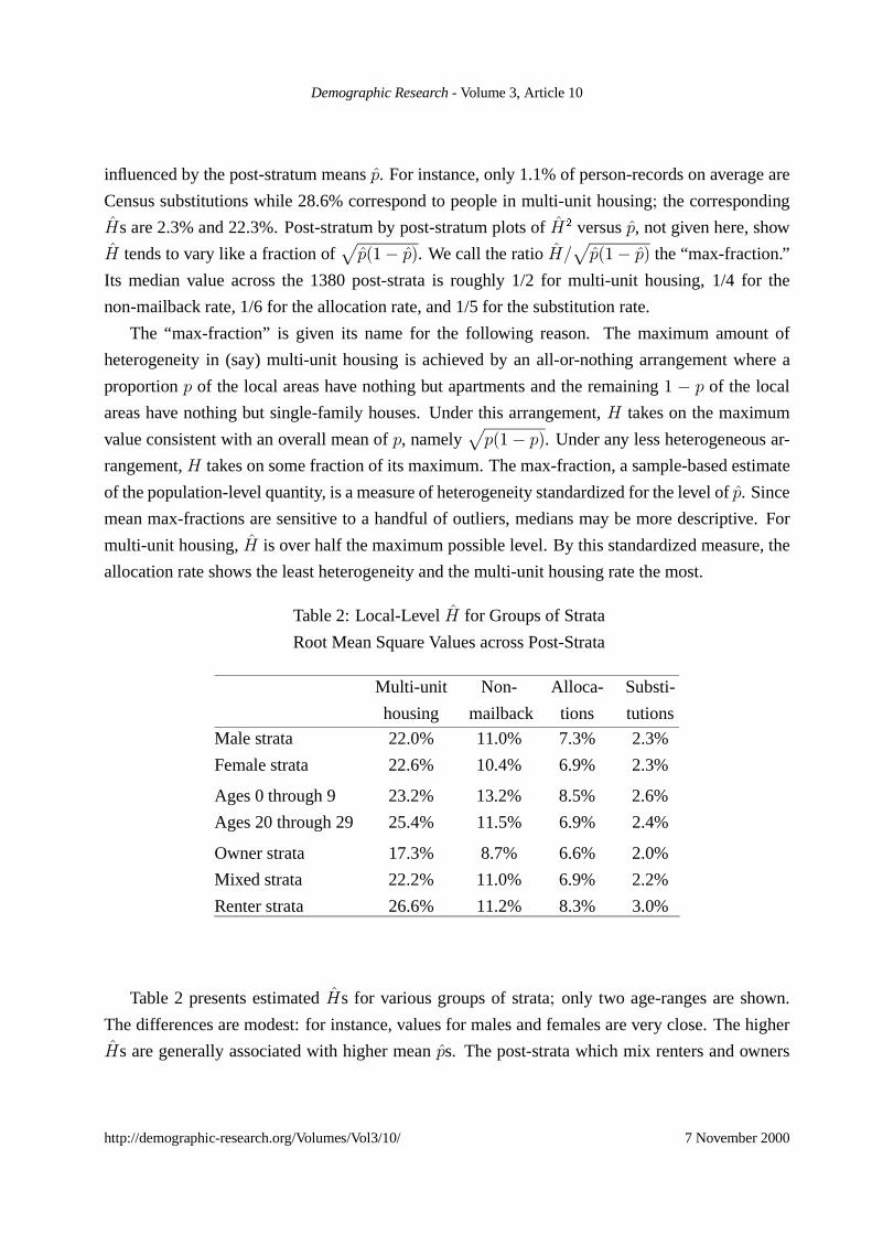
Table 2: Local-LevelM for Groups of Strata
Root Mean Square Values across Post-Strata
Multi-unit Non- Alloca- Substi-
housing mailback tions tutions
Male strata 22.0% 11.0% 7.3% 2.3%
Female strata 22.6% 10.4% 6.9% 2.3%
Ages 0 through 9 23.2% 13.2% 8.5% 2.6%
Ages 20 through 29 25.4% 11.5% 6.9% 2.4%
Owner strata 17.3% 8.7% 6.6% 2.0%
Mixed strata 22.2% 11.0% 6.9% 2.2%
Renter strata 26.6% 11.2% 8.3% 3.0%
Table 2 presents estimatedMs for various groups of strata� only two age-ranges are shown.
The differences are modest: for instance, values for males and females are very close. The higherMs are generally associated with higher meanRs. The post-strata which mix renters and owners
http://demographic-research.org/Volumes/Vol3/10/ 7 November 2000

Demographic Research - Volume 3, Article 10
together do not show more heterogeneity than the post-strata which separate out renters: the latter
strata have the higher meanRs.
Breakdowns by groups, like those in Table 2, show that heterogeneity is pervasive. Hetero-
geneity is not concentrated among post-strata of any particular type. Strata which mix groups like
owners and renters produce similar levels of heterogeneity as strata which separate them. That
outcome is further evidence that dependence on the details of post-strati¿cation is not severe. By
contrast, heterogeneity would be expected to vary with the geographical resolution. Table 3 showsMs from studies with different levels of resolution� the variable used is the allocation rate.
Table 3: Dependence ofM on Geographical Level for Allocations
Geography Data set Post-strata M
States within U.S. P-12 1392 2.9%
States within U.S. 1990 Census 357 3.9%
PUMAs within Oregon 1990 PUMS 120 6.6%
Localities within territories P-12 1392 7.1%
Sources: Table 1 in the present study for lines 1 and 4� [Freedman and Wachter
1994] for line 2� [Rhyne 1999] for line 3.
Table 3 has results for “Public Use Microdata Areas” (PUMAs), which are aggregations of
cities and counties into areas each of which contains at least 100,000 people. The results are due
to Marcey-Jo Rhyne and are quoted by permission. Her post-strati¿cation for the PUMAs follows
the one used in the 1990 PES, to the extent feasible: no distinctions of place-type can be made�
renters are distinguished from owners in all cases, as are blacks, non-black hispanics, Asian and
Paci¿c Islanders, and whites and others. She looked only at allocations. It is interesting that the
heterogeneity across the relatively large PUMA units within one state is nearly as high as the
heterogeneity across the much smaller local areas within larger territorial groupings.
http://demographic-research.org/Volumes/Vol3/10/ 7 November 2000
Demographic Research - Volume 3, Article 10
3 Applications to Census Undercount Estimation
The results of Section 2 provide guidance about the likely size of errors due to heterogeneity in the
Census Bureau’s small-area estimates of undercounts from the 1990 PES. They provide such guid-
ance to the extent that the P-12 variables provide meaningful analogues to undercounts with respect
to place-to-place variability, and to the extent that P-12 resembles the PES in sample design and
post-strati¿cation. The P-12 variables were chosen speci¿cally to provide such analogues. Like
undercounts, they are Census coverage indicators, and the Census Bureau goes so far as to call
them “proxies” or “surrogates” for undercount. The P-12 sample design was chosen to be essen-
tially the same as that for the PES, and the post-strati¿cations are identical. These considerations
all support the idea of taking P-12 as a guide to the effects of heterogeneity on 1990 undercount
estimates.
On the other hand, there is no direct validation of the posited similarity between P-12 variables
and undercounts. The main available comparisons are in terms of overall levels and indices of
dispersion. These are presented in this section. It turns out that undercounts fall well within the
range of alternatives spanned by the four P-12 variables, but no single P-12 variable is a close
match in both level and dispersion.
Net undercounts can be negative (when there is an overcount) but the P-12 variables are always
non-negative. This is an important difference which weakens the analogy. The net undercount
is approximately equal to the difference between two non-negative variables, the rates of “gross
omissions” (e.g., missed persons) and “erroneous enumerations” (e.g., duplicates or fabrications).
The P-12 variables may be better analogues for these two components of undercount than for their
difference, but the overall picture is complicated by the correlations between gross omissions and
erroneous enumerations which extend within post-strata all the way down to Census blocks.
Information on levels and indices of dispersion for undercount variables are shown in Table 4.
They are to be compared to the corresponding rows for P-12 variables in Table 1. In Table 4,
following common Bureau practice, centered adjustment factors are used in place of undercount
rates. The centered adjustment factor for any unit is calculated by taking the estimated true count,
dividing by the Census count, and subtracting one. The centered adjustment factor is close to the
undercount rate itself. The¿rst column in Table 4 pertains to the Bureau’s “smoothed” adjustment
factors, the factors actually used for the Bureau’s calculation of adjusted counts. The second
column pertains to the “raw” adjustment factors. These are dual-system estimates from PES data,
calculated post-stratum by post-stratum. The raw factors were transformed into the smoothed
factors by an empirical Bayes smoothing algorithm [Freedman et al. 1993]. The¿nal two columns
http://demographic-research.org/Volumes/Vol3/10/ 7 November 2000

Demographic Research - Volume 3, Article 10
pertain to the gross omission and erroneous enumeration rates. Neither Table 4 nor Table 1 is
weighted for post-stratum size.
Table 4: Comparative Values for PES Adjustment Factors
Smoothed Raw Gross Erroneous
Factors Factors Omissions EnumerationsStandard deviation
across post-strata 4.1% 7.0% 6.7% 4.5%
Mean of centered factors 2.8% 2.9% 9.7% 6.4%
RMS of Bureau’s
estimated standard errors 2.0% 5.9% unknown unknown
The level and dispersion of a variable undoubtedly affect the numerical values ofM for the
variable, so the comparisons between Table 1 and Table 4 are important indicators of the relevance
of P-12 to undercounts. With one exception, we see that all entries in Table 4 fall between the
corresponding values for substitutions and for allocations in Table 1. The exception is the 5.9%
sampling standard error for the raw factors, which falls above the standard error for allocations
and just below the high estimate of standard error for multi-unit housing. Thus, in terms of the
quantities shown in Table 4, the P-12 variables do span the relevant range, but none matches on all
dimensions.
An important conclusion is suggested by comparing the¿gure of 2.0% in the lower left of
Table 4 with the¿gures in the¿rst row of Table 1. The 2.0% is the RMS of the Bureau’s estimates
of sampling standard error for its smoothed adjustment factors, and it is lower than any of the
RMS values ofM for local areas in Table 1. If the P-12 variables are at all valid analogues, then
the estimated PES sampling variances are evidently dominated by the variance due to heterogeneity
measured byM2. Sampling variance is the contribution to error which the Bureau did include in
its error margins for adjusted local counts [U.S. Bureau of the Census 1991]. Variance due to
heterogeneity is one of the contributions it did not include. The data here suggest that what was
left out is more important than what was put in.
It is likely that some part of the true contribution from sampling variability was also left out.
http://demographic-research.org/Volumes/Vol3/10/ 7 November 2000

Demographic Research - Volume 3, Article 10
The 2.0% ¿gure for sampling standard deviation is believed to be a considerable underestimate
[Fay and Thompson 1993, Freedman et al. 1993]. In principle, sampling variance can be traded
off against variance due to heterogeneity by adopting a coarser or ¿ner post-strati¿cation. But the
variances due to heterogeneity implied by Table 1 are so large that the leeway for such tradeoffs
appears rather slight.
The particular use we are making of P-12, with our concentration on heterogeneity alone and
our direct calculation ofM within post-strata, avoids certain dif¿culties which would confront
more ambitious uses. We are not calculating measures of overall error for local counts or shares.
Thus we are not engaged in assessing the augmentations or cancellations of error that take place
when the positive or negative estimated adjustments for different post-strata in the same local area
are added together to yield the total estimate for the area. We cannot do so with P-12, because
P-12 superblocks for different post-strata do not coincide. Heterogeneity implies error both in
Census counts and in adjusted counts, and the balance between these errors appears to be a delicate
function of patterns of cancellation when post-stratum contributions are summed. We are also not
engaged in studying the interaction between errors in local counts due to heterogeneity and errors
at all levels due to bias in post-stratum-wide adjustment factors. We are studying errors in an
idealized, bias-free setting. This setting would correspond to a PES in which the post-stratum-
wide adjustment factors were known perfectly. Our counterparts of post-stratum-wide factors, that
is, ourRs, are unbiased.
The post-stratum-wide adjustment factors in the real PES are known to be biased. There is,
of course, some ratio-estimator bias. That is a side-effect of heterogeneity, and should be dis-
tinguished from the heterogeneity studied in this report, which affects estimated rates for local
areas within post-strata. There are other, more important, biases in the adjustment factors esti-
mated by the PES. Attempts have been made to measure some of these by quality-control and
followup studies, but only at the level of large aggregations of post-strata. Biases are quanti¿ed
in [Breiman 1994] and in Table 15 of the Census Bureau’s P-16 Project Report. Unfortunately,
this crucial table is omitted from the published version [Mulry and Spencer 1993]. There is also
unmeasured “correlation bias” resulting from the tendency for people missed by the Census to be
more likely to be missed by the PES estimates. Essentially nothing is known about how the mea-
sured biases are distributed among the post-strata, and even less about the size and distribution of
correlation bias. Thus there is not yet a basis on which de¿nitive assessments of the relative accu-
racy of adjusted and unadjusted counts for local areas could be made - unless some rather heroic
assumptions are to be imposed on the data. For recent reviews, see [Brown et al. 1999, Wachter
and Freedman 2000], but those¿ndings seem to be disputed in [Prewitt 2000].
http://demographic-research.org/Volumes/Vol3/10/ 7 November 2000

Demographic Research - Volume 3, Article 10
In short, at the local level, what can be made are assessments of components of error like
heterogeneity, not assessments of relative accuracy. To strengthen the assessments, it would be
valuable to relate P-12 more closely to the PES. The Census Bureau (as far as we can tell) has
not released data suf¿cient to calculate place-to-place correlations between the variables studied
here and undercounts. In principle, substitutions, allocations, non-mailback rates, and multi-unit
housing rates exist along with undercount estimates for the 5392 PES block clusters. Even more
relevant than such cross-correlations would be autocorrelation functions for the variables, calcu-
lated as functions of physical or notional distance between areas. The PES sample size is small for
this purpose, but some insights could be gleaned. At present, the correlations that can be computed
are those that are least relevant - across post-strata. Smoothed adjustment factors correlate 0.60
with non-mailback rates, 0.23 with multi-unit housing rates, 0.18 with substitution rates, and 0.07
with allocation rates, across post-strata. Substitution and allocation rates correlate 0.61 with each
other.
The PES sample is too small to give estimates of heterogeneity of the precision obtained from
P-12. At the local level, the data for anM calculation are not available to us at all for most post-
strata. At the state level, using weighted data by post-stratum and calculating as if the sampling
weights were uniform within post-strata, we¿nd RMS values forM for state-to-state heterogeneity
of 10% for gross omissions and 7% for erroneous enumerations. These¿gures fall near the upper
end of the RMS state-levelM values in Table 1. The PES estimates for single post-strata are
unstable to the extent that about 25% of post-strata come out with negative estimated values ofM2. The RMS values over all 1380 post-strata are bound to be more stable, and the¿gures suggest
that heterogeneity in components of undercount is at least as great as heterogeneity in the P-12
variables.
http://demographic-research.org/Volumes/Vol3/10/ 7 November 2000

Demographic Research - Volume 3, Article 10
4 Prior Literature
Notwithstanding the large literature on methods for small-area estimation, there have been com-
paratively few evaluation studies and even fewer attempts to quantify errors due to heterogeneity.
The literature on methods, building on [Deming 1948], is summarized by [Purcell and Kish 1979,
Platek et al. 1987, Ghosh and Rao 1994]. Uniform ratio estimators like the ones considered in
this study are the oldest and most widespread of all small-area estimators. They are sometimes
themselves called “synthetic estimators,” though that name, coined in [National Center for Health
Statistics 1968], is more properly applied when such estimators have been summed up within areas
over strata or groups.
Parametric evaluations based on variance-component models have been applied and studied
[Battese, Harter and Fuller 1988, Prasad and Rao 1990]. For that work, unlike P-12 and the
PES, each of the small areas for which estimates are needed contains sampled units� parameters
governing heterogeneity are identi¿able without the presence of a census or evaluation sample like
P-12. When direct comparisons and parametric estimates are not feasible, evaluations of small-area
estimates generally take the form of sensitivity analyses and simulation studies.
The literature on evaluation of small-area estimates tends to focus, like our report, on problems
of census adjustment. There is a simulation study of synthetic estimation using two demographic
groups [Schirm and Preston 1987]. The areas are states plus the District of Columbia� the variable
is the 1980 net Census undercounts. Lacking information about levels of heterogeneity of the kind
given in the present report, a stylized model is used. Group-speci¿c state effects are assumed to
be independent and identically distributed lognormal variables, with variances set to levels loosely
suggested by Census Bureau work on 1970 undercounts.
A form of evaluation that has come to be called “arti¿cial population analysis” has been
pursued with 1980 Census data [Isaki et al. 1987]. Related, as yet unpublished, work by Cen-
sus Bureau staff has been conducted with 1990 data. Both “across-the-board” (unstrati¿ed uni-
form ratio estimates) and synthetic estimates have been studied, also with 1980 data [Wolter and
Causey 1991]. The areas are states, counties, and 1980 Census enumeration districts (with typical
populations of a thousand or so). The variable under study is the Census substitution rate (also
studied in P-12), rescaled within strata to match certain 1980 national net undercount estimates.
The “across the board” studies use six strata de¿ned by place-type within New England. The syn-
thetic studies use 24 strata de¿ned by age, sex, and race within the whole United States. Results
are presented in terms of several aggregate “measures of closeness” for adjusted versus unadjusted
values. A discussion of these studies can be found in [Freedman and Navidi 1992].
http://demographic-research.org/Volumes/Vol3/10/ 7 November 2000

Demographic Research - Volume 3, Article 10
Using block-level data for components of undercount from the 1990 PES, within-group hetero-
geneity across blocks has been compared to within-block heterogeneity across groups [Hengartner
and Speed 1993]. In a study of Australian unemployment rates, small-area estimates are evaluated
by a direct comparison with tabulations from a contemporaneous census [Feeney 1987]. Our work
with P-12 is an approximate version of this direct strategy, in which an extra-large sample from
the census plays the role of the census itself.
The Bureau has analyzed the P-12 data, concentrating on the statistical signi¿cance of state-to-
state heterogeneity [Kim 1991, Kim, Blodgett and Zaslavsky 1993]. Several approaches were used,
including log-linear modeling of the P-12 variables, estimating state effects separately for post-
stratum groups. The test statistics measure excess heterogeneity from state to state after dividing
out the observed heterogeneity from local area to local area. This confounds the effects of local
heterogeneity with the effects of sample design. Given the high level of local heterogeneity, this
analytic strategy has little power for detecting state-to-state heterogeneity.
Methods like those of the present study have been applied to measure state-to-state heterogene-
ity in six Census coverage indicators including the four studied here [Freedman and Wachter 1994].
That work is based on the whole Census, not on a sample like P-12, and it uses a post-strati¿cation
with 357 strata instead of the 1392 used here. For various state-by-state tallies, the impact of
heterogeneity on loss-function analyses is quanti¿ed. The impact of other omitted or underesti-
mated sources of error on the Census Bureau’s loss function analyses for 1990 has been reviewed
[Freedman et al. 1994].
Previous investigators have detected residual heterogeneity in probabilities of enumeration by
the 1990 census [Alho et al. 1993]. The investigation focused on minorities in central cities across
the four census regions, and used logistic regression. One explanatory variable was the multi-unit
housing rate, which turned out to be strongly associated with capture in the census, at least in
two regions. Substitutions and allocations were excluded from the model, but were also strongly
associated with capture in the census. Overall, the impact of heterogeneity is estimated as being
roughly half the size of the net undercount. Geographic heterogeneity at state or substate levels
was not explicitly represented: the modeling was done at the level of individuals within broad
groups of post strata, some explanatory variables being de¿ned at the post-stratum level.
Many observers favor census adjustment� illustrative citations are [Schirm and Preston 1987,
Ericksen, Kadane and Tukey 1989, Wolter and Causey 1991, Mulry and Spencer 1993, Zaslavsky
1993, Belin and Rolph 1994, Steffey and Bradburn 1994, Anderson and Fienberg 1999, Cohen,
White and Rust 1999, Prewitt 2000]. Other observers¿nd that census adjustment would introduce
more error than it removes [Freedman and Navidi 1992, Hengartner and Speed 1993, Freedman et
http://demographic-research.org/Volumes/Vol3/10/ 7 November 2000
Demographic Research - Volume 3, Article 10
al. 1993, Breiman 1994, Freedman et al. 1994, Freedman and Wachter 1994, Brown et al. 1999,
Darga 1999, Wachter and Freedman 2000, Skerry 2000, Stark 2000]. There are a priori reasons to
favor adjustment� on the other hand, there are substantial biases in estimated adjustment factors,
and heterogeneity is pervasive. What is dif¿cult to determine from available data is the extent
to which biases reinforce each other or cancel, even at the state level� the bottom-line impact of
heterogeneity on accuracy is another major issue.
On the wider question of amounts of heterogeneity to be expected for variables of various kinds
at local levels, we are aware of no systematic empirical studies. The analysis of local Census data
as a¿eld of study is summed up by [Myers 1992]. Better empirical knowledge about geographical
heterogeneity in demographic behavior is important not only for small-area estimation but also
for the modeling of long-term demographic change. Parish-to-parish variability in English his-
torical data has been analyzed [Wachter 1992]. Stochastic demographic models which recognize
geographic levels of randomness in human population processes are the eventual goal.
http://demographic-research.org/Volumes/Vol3/10/ 7 November 2000
Demographic Research - Volume 3, Article 10
5 Conclusions
In summary, we have introduced a direct measure of heterogeneity, M , and used it to measure het-
erogeneity from local area to local area for four variables related to Census coverage. The source
of the data is the Census Bureau’s P-12 sample from the 1990 U.S. Census. The heterogeneity we
have measured is residual heterogeneity after strati¿cation by age, sex, race and ethnicity, renter-
owner status, place-type and broad geographical division of the country. The local areas are units
with total populations around 10,000. We¿nd that the area-to-area variance within strata - reÀect-
ing geographical heterogeneity - is roughly comparable to the variance from stratum to stratum,
even for this¿ne a strati¿cation.
The variables examined in this study are believed by the Census Bureau to offer meaningful
analogues to Census undercount. If this is true, then our results imply that errors due to hetero-
geneity from local area to local area dominate errors due to sampling variability in the small-area
ratio estimation step of the Bureau’s undercount estimates. The errors treated as negligible in the
calculation of error margins are larger than the errors included in the calculation. It follows that the
Census Bureau’s published margins of error for adjusted Census counts for local areas are likely
to be substantial underestimates.
For strati¿ed small-area ratio estimation, our results suggest that the popular “default option”
of treating residual heterogeneity as negligible is a serious mistake. When direct measures of error
due to heterogeneity are unavailable, a better default option would be to treat residual heterogeneity
as being on a par with the variance explained by the strati¿cation factors.
Variables like the P-12 rates can typically vary by 5, 10 or 20 percentage points from local area
to local area, even for people of the same age, sex, race, and ethnicity living in communities of the
same general size in the same broad areas of the country. In the absence of direct evidence to the
contrary, simulation studies of the ef¿cacy of small-area estimation should allow for substantial lo-
cal heterogeneity. “Diversity” is a byword in America’s political vocabulary. Diversity is certainly
the rule, when one looks from place to place across America with the Census Bureau’s 1990 P-12
sample.
http://demographic-research.org/Volumes/Vol3/10/ 7 November 2000

Demographic Research - Volume 3, Article 10
6 Acknowledgements
We thank the Donner Foundation for its ¿nancial support. The analysis has been carried out by us
with substantial assistance from Daniel Coster, Richard Cutler, Charles Everett, and Mark Hansen.
We are grateful to the U.S. Census Bureau for making the P-12 data available and for many helpful
explanations. We have served as consultants to the Freshpond Institute and as expert witnesses for
the government in litigation over proposed adjustments of the 1980 and 1990 censuses.
http://demographic-research.org/Volumes/Vol3/10/ 7 November 2000

Demographic Research - Volume3, Article10
References
Alho, J.M., M.H. Mulry, K. Wurdeman, and J. Kim (1993). “Estimating Heterogeneity in the
Probabilities of Enumeration for Dual System Estimation.” Journal of the American Statistical
Association, 88: 1130-36.
Anderson, M. and S.E. Fienberg (1999). Who Counts? The Politics of Census-Taking in Contem-
porary America. New York: Russell Sage Foundation.
Bateman, D. (1991). “Speci¿cations for Data Analysis of PES Project P12 Data.” Memorandum
Series #N-3, U.S. Bureau of theCensus, Washington, D.C.
Battese, G., R. Harter, and W.A. Fuller (1988). “An Error-Components Model for Prediction of
County Crop Areas Using Survey and Satellite Data.” Journal of the American Statistical Associ-
ation, 83: 28-36.
Belin, T.R. and J.E. Rolph (1994). “Can WeReach Consensuson CensusAdjustment?” Statistical
Science, 9: 486-508 (with discussion).
Breiman, L. (1994). “The 1990 Census Adjustment: Undercount or Bad Data?” Statistical Sci-
ence, 9: 458-475.
Brown, L.D., M.L. Eaton, D.A. Freedman, S.P. Klein, R.A. Olshen, K.W. Wachter, M.T. Wells,
and D. Ylvisaker (1999). “Statistical Controversies in Census2000.” Jurimetrics, 39: 347-375.
Cohen, M.L., A.A. White, and K.F. Rust, editors (1999). Measuring a Changing Nation: Modern
Methods for the 2000 Census. Washington, D.C.: National Academy Press.
Darga, K. (1999). Sampling and the Census, Washington, D.C.: TheAEI Press.
Deming, W.E. (1948). Statistical Adjustment of Data. New York: John Wiley and Sons.
Ericksen, E.P., J.B. Kadane, and J.W. Tukey (1989). “Adjusting the 1980 Census of Population
and Housing.” Journal of the American Statistical Association, 84: 927-944.
Fay, R. andJ. Thompson (1993). “The1990 Post EnumerationSurvey: Statistical Lessonsin Hind-
sight.” Proceedings of the 1993 Annual Research Conference of the U.S. Bureau of the Census.
Washington, D.C.: 71-91.
Feeney, G.A. (1987). “The Estimation of the Number of Unemployed at the Small Area Level.”
In Platek, R., J. Rao, C. Sarndal, and M. Singh, editors (1987). Small Area Statistics. New York:
John Wiley and Sons.
Freedman, D.A. and W.C. Navidi (1992). “Should We Have Adjusted the U.S. Census of 1980?”
Survey Methodology, 18: 3-74.
http://demographic-research.org/Volumes/Vol3/10/ 7 November 2000

Demographic Research - Volume 3, Article 10
Freedman, D.A., P.B. Stark, and K.W. Wachter (2000). “A Probability Model for Census Ad-
justment.” Mathematical Population Studies, to appear. Technical Report 557, Department of
Statistics, U.C. Berkeley.
Freedman, D.A. and K.W. Wachter (1994). “Heterogeneity and Census Adjustment for the Inter-
Censal Base.”Statistical Science, 9: 476-485, 527-537.
Freedman, D.A., K.W. Wachter, D. Coster, R.C. Cutler, and S.P. Klein (1993). “Adjusting the
Census of 1990: The Smoothing Model.”Evaluation Review, 17: 371-443.
Freedman, D.A., K.W. Wachter, R.C. Cutler, and S.P. Klein (1994). “Adjusting the U.S. Census of
1990: Loss Functions.”Evaluation Review, 18: 243-280.
Ghosh, M. and J.N.K. Rao (1994). “Small Area Estimation: An Appraisal.”Statistical Science, 9:
55-76.
Hengartner, N. and T.P. Speed (1993). “Assessing Between-Block Heterogeneity Within the Post-
strata of the 1990 Post-Enumeration Survey.”Journal of the American Statistical Association, 88:
1119-1125.
Hogan, H. (1993). “The 1990 Post-Enumeration Survey: Operations and Results.”Journal of the
American Statistical Association, 88: 1047-1061.
Isaki, C., G. Diffendal, and L. Schultz (1987). “Report on Statistical Synthetic Estimation for
Small Areas.” Technical Report 87-20, U.S. Bureau of the Census, Washington, D.C.
Kim, J. (1991). “P-12 Project Report.” U.S. Bureau of the Census, Washington, D.C.
Kim, J., R. Blodgett, and A. Zaslavsky (1993). “Evaluation of the Synthetic Assumption in the
1990 Post-Enumeration Survey.” Technical Report, U.S. Bureau of the Census, Washington, D.C.
Le Bras, Hervé (1993).La planète au village. Paris: Editions de l’Aube.
Mulry, M.H. and B.D. Spencer (1993). “Accuracy of 1990 Census and Undercount Adjustments.”
Journal of the American Statistical Association, 88: 1080-1091.
Myers, Dowell (1992).Analysis with Local Census Data. Boston: Academic Press.
National Center for Health Statistics (1968).Synthetic Estimates of Disability. Public Health
Service Publication No. 759, Washington, D.C.
Platek, R., J. Rao, C. Sarndal, and M. Singh, editors (1987).Small Area Statistics. New York:
John Wiley and Sons.
Prasad, N.G.N. and J. Rao (1990). “The Estimation of the Mean Squared Error of Small-Area
Estimators.”Journal of the American Statistical Association, 85: 163-171.
http://demographic-research.org/Volumes/Vol3/10/ 7 November 2000
Demographic Research - Volume 3, Article 10
Prewitt, K. (2000). “Accuracy and Coverage Evaluation� Statement of the Feasibility of Using
Statistical Methods To Improve the Accuracy of the Census 2000.”Federal Register 65, Tuesday
20 June 2000: 38374-38398.
Purcell, N.P. and L. Kish (1979). “Estimation for Small Domains.”Biometrics, 35: 365-384.
Rhyne, M. J. (1999). “Measuring Heterogeneity from Public Use Microdata Samples.” Senior
Thesis, Department of Statistics, U.C. Berkeley.
Schirm, A. and S. Preston (1987). “Census Undercount Adjustment and the Quality of Geographic
Population Distributions.”Journal of the American Statistical Association, 82: 965-983.
Skerry, P. (2000).Counting on the Census. Washington, D. C.: Brookings.
Stark, P.B. (2000). “The 1990 and 2000 Census Adjustment Plans.” Technical Report 550, De-
partment of Statistics, U.C. Berkeley.
Steffey, D.L. and N.M. Bradburn, editors (1994).Counting People in the Information Age. Wash-
ington, D.C.: National Academy Press.
Thompson, J. (1990). “Census Bureau Memorandum N-2 to Arnold Jackson.” U.S. Bureau of the
Census, Washington, D.C.
U.S. Bureau of the Census (1990). “Technical Operational Plans for the 1990 PES.” Washington,
D.C.
U.S. Bureau of the Census (1991). “Census Bureau Releases Re¿ned Estimates from Post- Enu-
meration Survey of 1990 Census Coverage.” Press Release (13 June 1991) CB91-221, Washington,
D.C.
Wachter, K.W. (1992). “Variabilité aléatoire des phenomènes démographiques: enseignements des
séries paroissiales de Wrigley et Scho¿eld.” In A. Blum, N. Bonneuil, and D. Blanchet, editors.
Modèles de la démographie historique. Paris: Institut National d’Etudes Démographiques, Presses
Universitaires de France.
Wachter, K.W. and D.A. Freedman (2000). “The Fifth Cell: Correlation Bias in U.S. Census
Adjustment.”Evaluation Review, 24: 191-211.
Wolter, K. and B. Causey (1991). “Evaluation of Procedures for Improving Population Estimates
for Small Areas.”Journal of the American Statistical Association, 86: 278-284.
Zaslavsky, A.M. (1993). “Combining Census, Dual System, and Evaluation Study Data to Esti-
mate Population Shares.”Journal of the American Statistical Association, 88: 1092-1105.
http://demographic-research.org/Volumes/Vol3/10/ 7 November 2000
Demographic Research - Volume3, Article10
Appendix
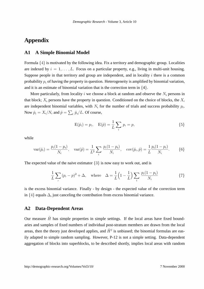
A1 A Simple Binomial Model
Formula iej is motivated by the following idea. Fix a territory and demographic group. Localities
are indexed by � ' �c � � � c u. Focus on a particular property, e.g., living in multi-unit housing.
Suppose people in that territory and group are independent, and in locality � there is a common
probability R� of having theproperty in question. Heterogeneity isampli¿ed by binomial variation,
and it is an estimateof binomial variation that is thecorrection term in i4j.
More particularly, from locality � we choose a block at random and observe the�� persons in
that block� f� persons have the property in question. Conditioned on the choice of blocks, thef�
are independent binomial variables, with �� for the number of trials and success probability R�.
Now R� ' f�*�� and R 'S
�R�*u. Of course,
,ER�� ' R�c ,ER� '�
u
[�
R� ' Rc iDj
while
�@hER�� 'R�E�� R��
��
c �@hER� '�
u2
[�
R�E�� R��
��
c UL�ER�c R� '�
u
R�E�� R��
��
� iSj
Theexpected valueof the naiveestimator i�j is now easy to work out, and is
�
u
[�
ER� � R�2 n{c ��ihi { '�
u
��� �
u
�[�
R�E�� R��
��
i.j
is the excess binomial variance. Finally - by design - the expected value of the correction term
in iej equals{, just canceling thecontribution from excess binomial variance.
A2 Data-Dependent Areas
Our measure M has simple properties in simple settings. If the local areas have ¿xed bound-
aries and samples of ¿xed numbers of individual post-stratum members are drawn from the local
areas, then the theory just developed applies, and M2 is unbiased� the binomial formulas are eas-
ily adapted to simple random sampling. However, P-12 is not a simple setting. Data-dependent
aggregation of blocks into superblocks, to be described shortly, implies local areas with random
http://demographic-research.org/Volumes/Vol3/10/ 7 November 2000

Demographic Research - Volume 3, Article 10
boundaries. The numbers of sampled individuals in these areas are themselves random, not ¿xed,
and that leaves the correction term in the de¿nition of M2 in need of justi¿cation. Sampling block
clusters instead of individuals introduces a term for cluster-level heterogeneity into the expecta-
tions. We sketch our treatment of the data-dependence¿rst and the term for clustered sampling
next.
The data-dependent boundaries turnR� andM into random quantities with expectations, and
the goal is to justify the formulas
,ER�� � ,ER�� @?_ ,E M2� � ,EM2� n�
u
[�
_�`�� iHj
In the display,`� accounts for within-area between-cluster covariance and_� is the analog of
a ¿nite-sample correction factor. Both are de¿ned below. We believe both are small, but our
argument is only heuristic, and that is one reason why our conclusions in this paper are somewhat
tentative.
The Census Bureau’s aggregation process, merging sample blocks into sample superblocks,
may be described as follows [Bateman 1991]. Within each post-stratum, after the P-12 sample
has been drawn, members are pooled together from block after block, following the sequence
of blocks in the sample list, until a minimum of ten members are included or a state boundary
is reached. Post-strata represent a¿ne-grained subdivision of the population along demographic
lines, so most blocks contain at most a handful of people from the same post-stratum. The stopping
rule for superblock completion typically puts half a dozen blocks into a superblock.
The list for the sampling frame snakes its way through the territory spanned by the post-stratum
from place to place among places of the same place type. The sampled blocks amalgamated into
one sample superblock are therefore often but not always drawn from the same contiguous area.
Superblocks are put together separately for each post-stratum and superblocks formed for different
post-strata do not coincide.
For our formal arguments, we use the word “locality” for the local area de¿ned to correspond
to a particular superblock in the following way. Split the ordered list of blocks in the sampling
frame randomly at a uniformly distributed point between the last sampled block in the previous
superblock and the¿rst sampled block in the current superblock. Repeat the procedure between the
current superblock and the succeeding one. That gives two breakpoints. The locality corresponding
to the current superblock is the set of all blocks in the list between the two breakpoints. The
superblock then equals the subset of blocks in the locality selected into the sample.
The order in the sampling frame maintains the integrity of address-register areas and Census
http://demographic-research.org/Volumes/Vol3/10/ 7 November 2000
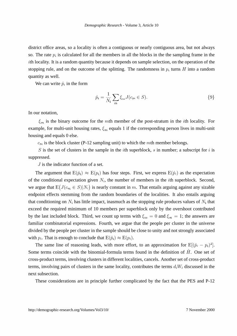
Demographic Research - Volume 3, Article 10
district of¿ce areas, so a locality is often a contiguous or nearly contiguous area, but not always
so. The rate R� is calculated for all the members in all the blocks in the the sampling frame in the
�th locality. It is a random quantity because it depends on sample selection, on the operation of the
stopping rule, and on the outcome of the splitting. The randomness in R� turns M into a random
quantity as well.
We can write R� in the form
R� '�
��
[6
16aES6 5 7�� ibj
In our notation,
16
is the binary outcome for the 6th member of the post-stratum in the�th locality. For
example, for multi-unit housing rates,16
equals 1 if the corresponding person lives in multi-unit
housing and equals 0 else.
S6 is the block cluster (P-12 sampling unit) to which the6th member belongs.
7 is the set of clusters in the sample in the�th superblock,r in number� a subscript for� is
suppressed.
a is the indicator function of a set.
The argument that,ER�� � ,ER�� has four steps. First, we express,ER�� as the expectation
of the conditional expectation given��, the number of members in the�th superblock. Second,
we argue that,�aES6 5 7�m��
�is nearly constant in6. That entails arguing against any sizable
endpoint effects stemming from the random boundaries of the localities. It also entails arguing
that conditioning on�� has little impact, inasmuch as the stopping rule produces values of�� that
exceed the required minimum of 10 members per superblock only by the overshoot contributed
by the last included block. Third, we count up terms with16
' f and16
' �� the answers are
familiar combinatorial expressions. Fourth, we argue that the people per cluster in the universe
divided by the people per cluster in the sample should be close to unity and not strongly associated
with R�. That is enough to conclude that,ER�� � ,ER��.
The same line of reasoning leads, with more effort, to an approximation for,dER� � R��2o.
Some terms coincide with the binomial-formula terms found in the de¿nition of M. One set of
cross-product terms, involving clusters in different localities, cancels. Another set of cross-product
terms, involving pairs of clusters in the same locality, contributes the terms_�`� discussed in the
next subsection.
These considerations are in principle further complicated by the fact that the PES and P-12
http://demographic-research.org/Volumes/Vol3/10/ 7 November 2000

Demographic Research - Volume3, Article10
samples are strati¿ed samples with some variation in sampling weights. Sampling stratum mem-
bership is not indicated in the P-12 dataset. Sampling strata and sampling weights have major
effects in the PES, but we expect their effects in P-12 to be minor for several reasons, including
theabsenceof movers, the lack of non-responsereweighting and special small-block samples, and
the fact that our R and R are not weighted averages but simpleaverages across localities.
A3 Effects of Clustered Sampling
The P-12 sample is a clustered sample primarily because individuals are clustered into blocks
and secondarily because blocks are clustered into block clusters (containing one or two blocks in
most cases). In the presence of clustered sampling, heterogeneity from cluster to cluster within
localities makes a downweighted but nonzero contribution to sampling variability inS
ER� � R�2
and introduces, as we have said, a term of the form _�`� into ,E M2�. The average within-cluster
covariance in theuniverseof membersof the �th locality is given by
`� '� [6�'6�
Ef6 � R��Ef6� � R��aES6 ' S6� 5 L��1�[
S
�SE�S � ���� i�fj
The sums range over all clusters in the �th locality, and �S is the number of members in the Sth
block cluster. The denominator is the number of terms in the numerator. For the contribution to
sampling variability, `� must bemultiplied by _�, where
_� ' ,�[
S
�SE�S � ���1�
��
[S
�S
�� i��j
If members of thepost-stratum werespread out with onemember per cluster, _� would bezero. If
each cluster always had 10 members, forcing �S ' �� ' �f under the stopping rule and creating
single-cluster superblocks, _� would be9/10. (With our notation, if the�th superblock in thesample
has index S in thesampling frame, then�� ' �S.)
The covariance factor `� measures how much more often the outcomes for two members
of the same cluster agree compared to the outcomes for two randomly chosen members of the
whole locality. At the extreme, each cluster could consist entirely of ones or entirely of zeros,
irrespective of size, and then we would have`� ' R�E� � R��, the variance of the outcome for a
single randomly-selected member of the locality. Thedownweighting _� would scale thisvariance
by akind of effectivesamplesizefor theclustered sampling. Usually, however, knowingf6 gives
only limited information about f6�, and`� wil l beclose to zero.
http://demographic-research.org/Volumes/Vol3/10/ 7 November 2000

Demographic Research - Volume3, Article10
The only non-zero contributions to `� come from clusters with two or more members� large
contributions only from clusters with many members. Clusters with many members appear to
be rare. The identity of blocks is erased in the P-12 data set� however, we have detailed census
and PES data for metropolitan areas outside central cities in the Paci¿c division, nicknamed the
“Berkeley dataset.” In thesedata, of theclusters that contain any post-stratum member, about 20%
contain only onesuch person. (Weareaveraging over post-strata.) Another 16% contain 2 people,
and only about 20% contain 7 or more. The_� factors averageout near 1/2.
We cannot measure `� directly from P-12, and the PES sample is much too small for sta-
ble estimates. There is, however, an empirical test of the extreme hypothesis that all or most of
the observed values of M2 are contributed by within-cluster covariances. Under this hypothesis,
`� would not increase as localities and superblocks are merged into superlocalities and supersu-
perblocks, and _� would decrease in accordance with the formula i��j. Values of M have been
inspected under a sequence of mergings for selected post-strata: M falls off substantially more
slowly than its predicted value under this extreme hypothesis. Any other outcome would be sur-
prising� thesmall numbers of post-stratum members per cluster makes thesampling quiteclose to
random sampling of individualsand thus to thecasewhere thewithin-cluster covariancecontribu-
tion is absent.
Bothbetween-locality heterogeneity andbetween-cluster within-locality heterogeneity areforms
of heterogeneity. M remains a measure of heterogeneity whether or not the`� contributions are
small. But between-locality heterogeneity is of primary interest� it is the contribution which di-
rectly affects estimates for whole local areas. The arguments in this section support the view that
in the P-12 data set the approximation ,E M2� � ,EM2� is a workable one, and that the values in
Table1 are principally to be interpreted as evidenceof heterogeneity from locality to locality.
A4 The Standard Errors for Table 1
ThenineCensusdivisions represent, with ahandful of exceptions, disjoint groups in thesampling
schemeand their RMS M2s areessentially independent of each other. Thesquared measureM2 in
Table 1 is the weighted mean of the nine M2s for the divisions, weighting by the number of post-
strata in each division. For our calculation wemaketheassumption that theexpected valuesof the
nine measures for the divisions are all the same (cf. Table 4), while the nine variances differ. We
writedown an unbiased estimator for thevarianceof theoverall measureasaweighted averageof
thesquared deviationsof thedivisional measuresfrom theoverall weighted mean. Theweightsare
functions of the numbers of post-strata in the divisions. This estimate should be something of an
http://demographic-research.org/Volumes/Vol3/10/ 7 November 2000

Demographic Research - Volume 3, Article 10
upper bound, because part of the variability in divisional measures must reÀect small differences
among expected values rather than sampling variability as assumed. We convert to square roots
with a delta-method approximation.
Two alternative estimates for the sampling standard errors inR are given in Table 1. An indirect
approach is required because the identity of the sampling units has been erased by the superblock
aggregation process� to our knowledge, the Census Bureau has not published direct estimates of
standard errors for P-12. The low estimate in Table 1 is obtained by treating individuals as if
they were the sampling units� the sampling variance for a post-stratum-wideR is then computed as
RE� � R�*ES
���. The high estimate treats superblocks as if they were the sampling units. Then
the sampling variance is computed as
�
uEu� ��
[�
ER� � R�2c
whereu is the number of super-blocks associated with the post-stratum in question. These esti-
mates apply to P-12 itself� ¿nally, we rescale in proportion to sample size, as measured by block
clusters.
http://demographic-research.org/Volumes/Vol3/10/ 7 November 2000