Measuring Differential Gain and Phase - Texas … Differential Gain and Phase Randy Stephens Mixed...

Application ReportSLOA040 - November 1999

1

Measuring Differential Gain and PhaseRandy Stephens Mixed Signal Products

ABSTRACT

Standard video signals are based on a system developed in the 1950’s. The colors andbrightness we see on a television screen are encoded within an analog signal. How well anamplifier reproduces this video signal is the foundation for the measurement of differentialgain and phase.

The topic of this discussion is the basic concept of differential gain and phase. This discussionwill then lead to the analysis of the method used by Texas Instruments to measure differentialgain and phase for the high speed amplifier product line—the THS family.

Contents

1 Introduction 2. . . . . . . . . . . . . . . . . . . . . . . . . . . . . . . . . . . . . . . . . . . . . . . . . . . . . . . . . . . . . . . . . . . . . . . . .

2 Differential Gain and Phase Definitions 2. . . . . . . . . . . . . . . . . . . . . . . . . . . . . . . . . . . . . . . . . . . . . . . .

3 Differential Gain and Phase Test Setup 3. . . . . . . . . . . . . . . . . . . . . . . . . . . . . . . . . . . . . . . . . . . . . . . .

4 Testing Differential Gain and Phase 7. . . . . . . . . . . . . . . . . . . . . . . . . . . . . . . . . . . . . . . . . . . . . . . . . . .

5 Summary 11. . . . . . . . . . . . . . . . . . . . . . . . . . . . . . . . . . . . . . . . . . . . . . . . . . . . . . . . . . . . . . . . . . . . . . . . . . .

Appendix A A Primer for the Composite Video Signal 12. . . . . . . . . . . . . . . . . . . . . . . . . . . . . . . . . . . . A.1 Definitions 12. . . . . . . . . . . . . . . . . . . . . . . . . . . . . . . . . . . . . . . . . . . . . . . . . . . . . . . . . . . . . . . . . . . . . A.2 Creating the Composite Video Signal 15. . . . . . . . . . . . . . . . . . . . . . . . . . . . . . . . . . . . . . . . . . . . . .

List of Figures

1 Differential Gain and Phase Test Signal 4. . . . . . . . . . . . . . . . . . . . . . . . . . . . . . . . . . . . . . . . . . . . . . . . . . . . 2 Differential Gain and Phase Test Setup 5. . . . . . . . . . . . . . . . . . . . . . . . . . . . . . . . . . . . . . . . . . . . . . . . . . . . 3 Actual Differential Gain and Phase Results (4 lines = 37.5 Ω) 8. . . . . . . . . . . . . . . . . . . . . . . . . . . . . . . . . 4 Actual Differential Gain and Phase Results (2 lines = 75 Ω) 9. . . . . . . . . . . . . . . . . . . . . . . . . . . . . . . . . . . 5 Base-Line Results After System Calibration 10. . . . . . . . . . . . . . . . . . . . . . . . . . . . . . . . . . . . . . . . . . . . . . . A–1 A Typical 75%-Amplitude, 100%-Saturation Composite Video Signal 12. . . . . . . . . . . . . . . . . . . . . . A–2 Frequency Interleaving Spectrum 14. . . . . . . . . . . . . . . . . . . . . . . . . . . . . . . . . . . . . . . . . . . . . . . . . . . . . A–3 NTSC Composite Video Frequency Spectrum 14. . . . . . . . . . . . . . . . . . . . . . . . . . . . . . . . . . . . . . . . . . A–4 Vector Diagram 18. . . . . . . . . . . . . . . . . . . . . . . . . . . . . . . . . . . . . . . . . . . . . . . . . . . . . . . . . . . . . . . . . . . . . A–5 Chrominance Signal Components 19. . . . . . . . . . . . . . . . . . . . . . . . . . . . . . . . . . . . . . . . . . . . . . . . . . . . A–6 The Construction of an NTSC Composite Video Signal 20. . . . . . . . . . . . . . . . . . . . . . . . . . . . . . . . . .

List of Tables

1 AUT Loads for Measuring Differential Gain and Phase 6. . . . . . . . . . . . . . . . . . . . . . . . . . . . . . . . . . . . . . . A–1 75% Amplitude, 100% Saturation NTSC Color Bars 21. . . . . . . . . . . . . . . . . . . . . . . . . . . . . . . . . . . . . . A–2 100% Amplitude, 100% Saturation NTSC Color Bars 21. . . . . . . . . . . . . . . . . . . . . . . . . . . . . . . . . . . . .

SLOA040

2 Measuring Differential Gain and Phase

1 Introduction

Composite video contains the two parts of the video signal—the subcarrier portion and abroadband portion. The broadband portion of the composite video signal controls the brightness,or luminance, of the picture to be displayed. The subcarrier portion of the composite video signalcontrols the color, or chrominance, of the picture to be displayed. In turn, this color informationhas two parts to it: the amplitude and the phase. Together, all of these constitute what we see onour television or monitor screens. If any part of the signal is not reproduced correctly, the picturewill not be displayed correctly. It could show sunny images as night scenes, or it could show thebright yellow sun as a blue sphere.

One of the most critical factors within a composite video system is how well an amplifierreproduces the composite video signal. A series of tests were conducted to verify if anoperational amplifier is useful for video signals. These are called differential gain and phasetests. Even though this is a standardized specification for all manufacturers data sheets, noteveryone does it the same way.

Because video information can cover a range from 0 Hz to 6 MHz or greater, the amplifier musthave a frequency response of at least 50 MHz to 60 MHz. This precludes the vast majority ofamplifiers, and typically leaves the high-speed amplifier product group as the only viable solutionfor amplifiers within a video system. It may be best to start with the definitions for differential gainand phase.

2 Differential Gain and Phase Definitions

Differential gain is the error in the amplitude of the color signal due to a change in luminance(brightness) level. Basically, the subcarrier reference signal (3.58 MHz or 4.43 MHz) is beingoffset by a low-frequency ramp going from 0 IRE (0 V) to 100 IRE (714 mV). This signal is thenfed through an amplifier configured for a gain of +2 with a fixed load resistance (typically 150 Ω).The change in the amplitude of the subcarrier reference signal being offset by the ramp is calleddifferential gain error. It is usually expressed as a percent error.

Differential gain is important to video signals because if the amplitude of the subcarrier signalchanges with a change in luminance level, then the picture being displayed will have colorsaturation problems. A color with 100% saturation is commonly called a deep color. A deep redball being displayed with bright lights shining on it should not turn dull red when the lights start todim. It may turn dull red if the saturation level of the base color (red) decreases as the luminancelevel decreases.

Differential phase is the error in the phase of the color signal due to a change in luminance(brightness) level. The phase of the color signal is responsible for displaying the proper hue, orbase color. This measurement follows the exact same procedure as the differential gainmeasurement, but only looks for the change in phase of the subcarrier reference signal as theoffset level changes. Differential phase is usually expressed in degrees.

Differential phase is important to video signals because if the phase of the subcarrier signalchanges with a change in luminance level, then the picture being displayed will have colorselection problems. For example, a red ball being displayed with bright lights shining on it shouldnot turn orange when the lights start to dim. It may turn orange if the base color informationstarts to add some green to the image.

SLOA040


Typically, the human eye cannot discern the difference of color saturation if the differential gainerror is 1% or lower. Additionally, the human eye cannot discern a hue error of less than 1%. Ifthis is true, then why would anyone want an amplifier with less than 0.5% differential gain orphase error? The reasoning is that there can be several amplifiers along the video signal path.Cascading multiple amplifiers adds both positive and negative differential gain and differentialphase errors together. A typical video system will consist of the recording equipment, thetransmitter, the receiver, and the display device. So, if there are 20 amplifiers in the entire videosignal chain, with each one having a 0.1% differential gain and phase error, then it is probablethat the total system will have a differential gain and phase error of 20 × 0.1% or 2%. This is waytoo high for a good system, not to mention a studio quality system.

3 Differential Gain and Phase Test Setup

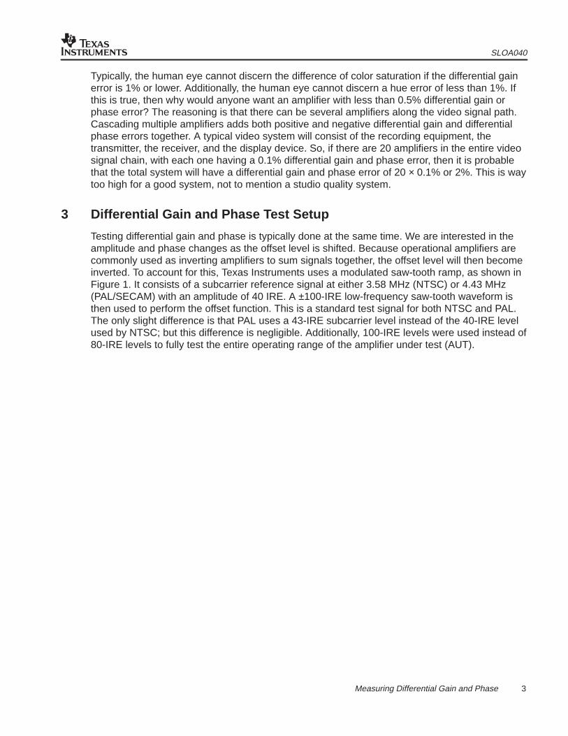
Testing differential gain and phase is typically done at the same time. We are interested in theamplitude and phase changes as the offset level is shifted. Because operational amplifiers arecommonly used as inverting amplifiers to sum signals together, the offset level will then becomeinverted. To account for this, Texas Instruments uses a modulated saw-tooth ramp, as shown inFigure 1. It consists of a subcarrier reference signal at either 3.58 MHz (NTSC) or 4.43 MHz(PAL/SECAM) with an amplitude of 40 IRE. A ±100-IRE low-frequency saw-tooth waveform isthen used to perform the offset function. This is a standard test signal for both NTSC and PAL.The only slight difference is that PAL uses a 43-IRE subcarrier level instead of the 40-IRE levelused by NTSC; but this difference is negligible. Additionally, 100-IRE levels were used instead of80-IRE levels to fully test the entire operating range of the amplifier under test (AUT).

SLOA040


Amplitude = 40 IRE

T = 1.1 Seconds

Subcarrier Signal :NTSC = 3.58 MHz

PAL/SECAM = 4.43 MHz

0 Volts

– 10

0 IR

E+

100

IRE

Figure 1. Differential Gain and Phase Test Signal

Some test setups use a staircase ramp instead of the linear ramp. The problem with a staircaseramp is that it does not measure every point. Differential gain and phase errors are not usuallyproportional to the offset level. In fact, it has been observed on numerous occasions that themaximum errors occurred somewhere between the two end points and not at the ends of theramp. Considering the unpredictability of the amplifier, discrete steps may not give a truerepresentation of the real differential gain and phase errors.

To accomplish the test using this waveform and to perform the analysis of the operationalamplifier, an HP8753D (or E) network analyzer was chosen. An HP3325A function generator isthen connected into the bias input port of the network analyzer (see Figure 2). To keepeverything correctly timed, the sync output of the function generator is connected to the syncinput of the network analyzer. The HP3325A generates the low-frequency saw-tooth waveform,while the HP8753D (or E) applies the high-frequency reference signal (3.58 MHz or 4.43 MHz)on top of the saw tooth. The HP3325A function generator was chosen because it is notinfluenced by the high-frequency signal being generated by the network analyzer. It was foundthat other function-generator outputs would be influenced by the subcarrier frequency and wouldcause the saw-tooth waveform to behave unpredictably.

SLOA040


+

–

AUT

22 µF

0.1 µF

+VCC

0.1 µF

22 µF

–VCC

RL

RG

RF

50 Ω

VOUT

RSVNA

Port 2Port 1

HP8753D (or E)NetworkAnalyzer

HP3325AFunctionGenerator

Sync

Signal

VIN

Figure 2. Differential Gain and Phase Test Setup

The AUT is usually set up with a gain of +2 (RF = RG). This is done because most videosystems, not to mention most transmission-line systems, use double termination on the amplifieroutput. When a double termination is performed, the signal amplitude at the receiving side isreduced by a factor of two. To compensate for this, the driving amplifier is set to a gain of +2.

Although it is realistic to see an amplifier in the inverting configuration, the differential gain andphase tests are done in the noninverting configuration. There are two reasons for this: first, thenoise gain of an amplifier is always referred to the noninverting input; so an amplifier set to again of –1 is equivalent to a gain of +2 configuration when it comes to amplifier noise gain; thesecond reason is that a noninverting configuration should theoretically have worse errors thanan inverting configuration because the input terminals of the amplifier are held at a fixedreference point (a virtual ground for the inverting terminal). But, in the noninverting gain of +2configuration, the amplifier’s input-circuitry voltage fluctuation is directly proportional to theapplied input-signal voltage. If the voltage of the amplifier’s input circuitry changes, there is moreroom for errors to occur due to the reduced common-mode rejection ratio of the op-amp. Forthese reasons, the AUT is tested with a gain of +2 to provide the worst-case conditions for errorsto occur.

SLOA040


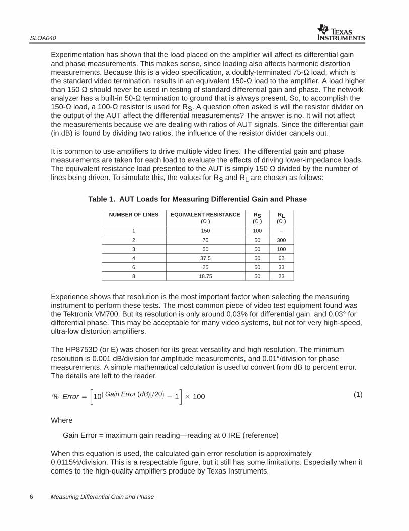
Experimentation has shown that the load placed on the amplifier will affect its differential gainand phase measurements. This makes sense, since loading also affects harmonic distortionmeasurements. Because this is a video specification, a doubly-terminated 75-Ω load, which isthe standard video termination, results in an equivalent 150-Ω load to the amplifier. A load higherthan 150 Ω should never be used in testing of standard differential gain and phase. The networkanalyzer has a built-in 50-Ω termination to ground that is always present. So, to accomplish the150-Ω load, a 100-Ω resistor is used for RS. A question often asked is will the resistor divider onthe output of the AUT affect the differential measurements? The answer is no. It will not affectthe measurements because we are dealing with ratios of AUT signals. Since the differential gain(in dB) is found by dividing two ratios, the influence of the resistor divider cancels out.

It is common to use amplifiers to drive multiple video lines. The differential gain and phasemeasurements are taken for each load to evaluate the effects of driving lower-impedance loads.The equivalent resistance load presented to the AUT is simply 150 Ω divided by the number oflines being driven. To simulate this, the values for RS and RL are chosen as follows:

Table 1. AUT Loads for Measuring Differential Gain and Phase

NUMBER OF LINES EQUIVALENT RESISTANCE(Ω )

RS(Ω )

RL(Ω )

1 150 100 –

2 75 50 300

3 50 50 100

4 37.5 50 62

6 25 50 33

8 18.75 50 23

Experience shows that resolution is the most important factor when selecting the measuringinstrument to perform these tests. The most common piece of video test equipment found wasthe Tektronix VM700. But its resolution is only around 0.03% for differential gain, and 0.03° fordifferential phase. This may be acceptable for many video systems, but not for very high-speed,ultra-low distortion amplifiers.

The HP8753D (or E) was chosen for its great versatility and high resolution. The minimumresolution is 0.001 dB/division for amplitude measurements, and 0.01°/division for phasemeasurements. A simple mathematical calculation is used to convert from dB to percent error.The details are left to the reader.

% Error 10Gain Error (dB) 20 1 100

Where

Gain Error = maximum gain reading—reading at 0 IRE (reference)

When this equation is used, the calculated gain error resolution is approximately0.0115%/division. This is a respectable figure, but it still has some limitations. Especially when itcomes to the high-quality amplifiers produce by Texas Instruments.

(1)

SLOA040


4 Testing Differential Gain and Phase

To properly measure differential gain and phase, the test setup should be calibrated first. This isaccomplished by first adjusting both channels of the HP8753D (or E) network analyzer to thefollowing settings:• Sweep type = CW time• CW frequency = 3.58 MHz (or 4.43 MHz)• Power = –6.9 dBm (40 IRE)• IF = 300 Hz• Number of data points = 401• Averaging factor = 20 (sometimes higher, depending on signal)• Smoothing factor = 1% to 5% (depending on amplitude)• External trigger on sweep

The HP3325A function generator is then adjusted to the following settings:

• Frequency = 0.905 Hz• Amplitude = 1.428 VPP (± 100 IRE)• Offset = 0 V• Function = saw tooth

Once this setup is complete, the output cable on port 1 is connected to the input cable on port 2with a double female SMA adapter. The network analyzer is set to calibrate mode and allowed tocalibrate itself. Then the AUT circuit is place in the test path as shown in Figure 2.

The tests are conducted for both the NTSC subcarrier at 3.58 MHz, and the PAL subcarrier at4.43 MHz. Additionally, the AUT’s power-supply voltages are run at ±15 V and ±5 V at eachsubcarrier frequency. All of these tests are then repeated using the equivalent loads specified inTable 1. The network analyzer is recalibrated whenever the subcarrier frequency is changed toensure reliable measurement results.

Once all of the data is taken, the differential gain and phase numbers are extracted. Becausedifferential gain and phase are measurements of error caused by a change in offset voltage,Texas Instruments looks only for the largest change along each of the ±100 IRE signals with thereference signal level at 0 IRE (0 V). The largest difference on gain may be on the +100-IREmagnitude, and on the –100-IRE magnitude for phase. It does not matter where it is, we aresimply looking for the worst-case condition. The differential gain error is calculated by usingformula (1) for the absolute-maximum difference in gain signal. The differential-phase error iscalculated by simply subtracting the absolute-maximum difference from the reference value.

Depending on the signal coming through the setup, the number of averages may need to beincreased. This is done specifically when the network analyzer is at its highest resolutionsettings (0.001 dB and 0.01°). The signal may be very choppy, and increasing the averages willtend to average out random noise from the system.

For very low distortion amplifiers driving a 150-Ω load, the error signal may still be too hard tosee. This is where the smoothing function plays a role. Smoothing computes a displayed datapoint based on a moving average of several adjacent points. Its function is to reduce relatively-small peak-to-peak noise values in the measured data. The minimum smoothing value is used

SLOA040


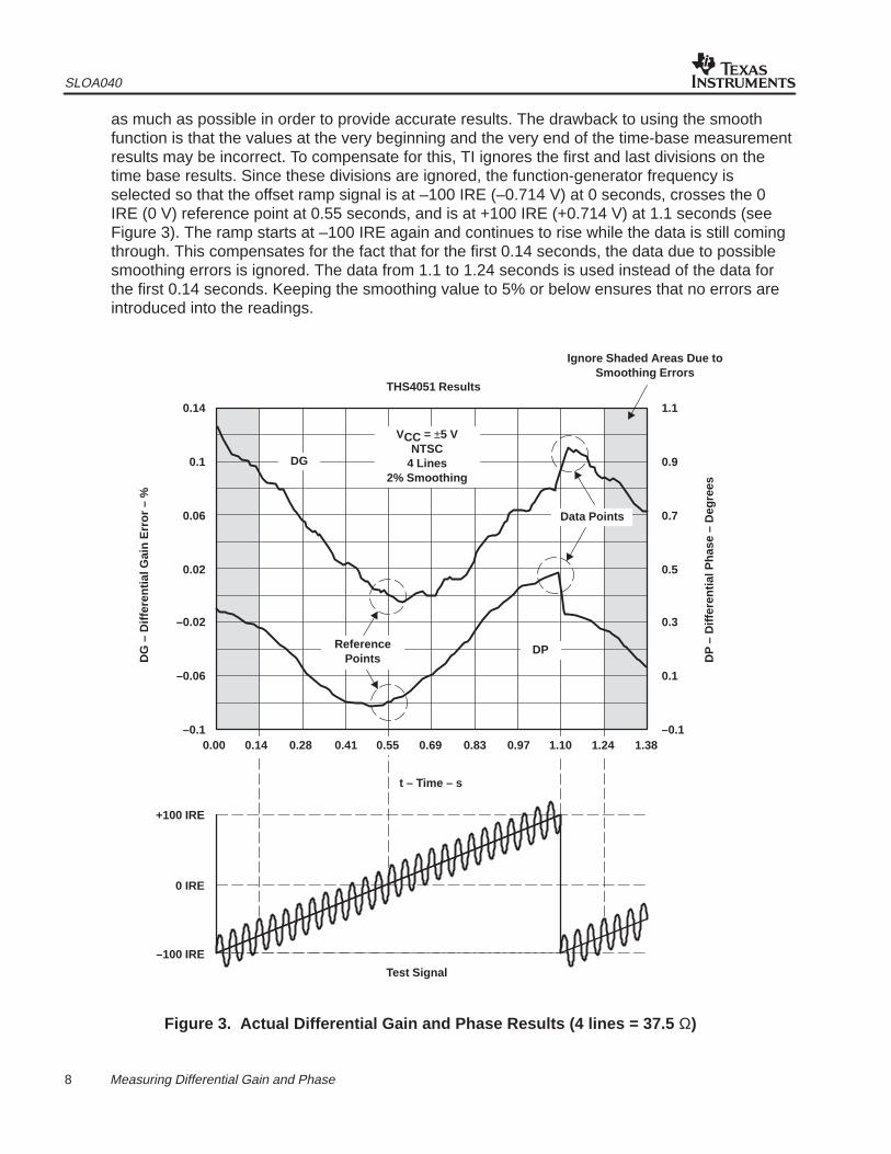
as much as possible in order to provide accurate results. The drawback to using the smoothfunction is that the values at the very beginning and the very end of the time-base measurementresults may be incorrect. To compensate for this, TI ignores the first and last divisions on thetime base results. Since these divisions are ignored, the function-generator frequency isselected so that the offset ramp signal is at –100 IRE (–0.714 V) at 0 seconds, crosses the 0IRE (0 V) reference point at 0.55 seconds, and is at +100 IRE (+0.714 V) at 1.1 seconds (seeFigure 3). The ramp starts at –100 IRE again and continues to rise while the data is still comingthrough. This compensates for the fact that for the first 0.14 seconds, the data due to possiblesmoothing errors is ignored. The data from 1.1 to 1.24 seconds is used instead of the data forthe first 0.14 seconds. Keeping the smoothing value to 5% or below ensures that no errors areintroduced into the readings.

Test Signal

+100 IRE

–100 IRE

0 IRE

t – Time – s

0.00 0.14 0.28 0.41 0.55 0.69 0.83 0.97 1.10 1.24 1.38

VCC = ±5 VNTSC

4 Lines2% Smoothing

ReferencePoints

Data Points

DP

DG

–0.1

–0.06

–0.02

0.02

0.06

0.1

0.14

–0.1

0.1

0.3

0.5

0.7

0.9

1.1

DP

– D

iffer

entia

l Pha

se –

Deg

rees

DG

– D

iffer

entia

l Gai

n E

rror

– %

Ignore Shaded Areas Due toSmoothing Errors

THS4051 Results

Figure 3. Actual Differential Gain and Phase Results (4 lines = 37.5 Ω)

SLOA040


Figure 3 shows the data points used to find the actual differential gain and phase numbers.These include the 0-IRE reference point and the maximum deviation from each reference point,as indicated in the graph. This graph shows that the worst-case differential gain occurred at–100 IRE (0.11%), and the worst-case differential phase occurred at +100 IRE (0.5°). It does notmatter where the maximum error point is relative to the IRE level; only the maximum errorrelative to the reference points is relevant. For example, the same amplifier was tested with only2 lines (75-Ω equivalent load). The maximum differential-gain error just happened to occur at+100 IRE (0.02%), and the maximum differential phase error occurred at +100 IRE (0.075°).

0.00 0.14 0.28 0.41 0.55 0.69 0.83 0.97 1.10 1.24 1.38

VCC = ±5 VNTSC

2 Lines4% Smoothing

DP

DG

–0.04

–0.03

–0.02

–0.01

0

0.01

0.02

–0.1

–0.05

0

0.05

0.1

0.15

0.2

DP

– D

iffer

entia

l Pha

se –

Deg

rees

DG

– D

iffer

entia

l Gai

n E

rror

– %

Ignore Shaded Areas Due toSmoothing Errors

THS4051 Results

Data Points

ReferencePoints

t – Time – s

Figure 4. Actual Differential Gain and Phase Results (2 lines = 75 Ω)

There are two network-analyzer settings that may need additional explanation—the 401 datapoints and the 300-Hz IF bandwidth. The number of data points was selected so that enoughpoints were taken to allow the smoothing factor to average out any random noise within theentire system. If enough data is collected, then random noise should average to a specific level.This level is subtracted from the AUT measurement by the network analyzer after calibration.This subtraction factor should become more consistent from test-to-test as the number of datapoints is increased. Misleading results will occur if the number of data points is too small.

SLOA040


The 300-Hz IF bandwidth was selected to allow the measurement of extremely small errors.Lowering the IF bandwidth from the network analyzer’s default setting of 3,000 Hz will lower thenoise floor of the system by about 10 dB. Additionally, lowering the IF bandwidth is better thanaveraging because it filters out spurious responses, odd harmonics, higher-frequency spectralnoise, and line-related noise. When we are looking at operational amplifiers with differential gainand phase errors better than 0.01% and 0.01°, respectively, any reduction in system noise isextremely valuable. The drawback of lowering the IF bandwidth is a dramatic increase in theamount of time required to make one sweep. But this is a small price to pay for good results.

The base-line data in Figure 5 show the actual results after calibrating the system and bypassingthe AUT. This was taken with 5% smoothing and 25 averages. The maximum differential gainerror shown is 0.0034%, and the maximum differential phase error is 0.0027°.

0.00 0.14 0.28 0.41 0.55 0.69 0.83 0.97 1.10 1.24 1.38

DP

DG

–0.008

–0.006

–0.004

0

0.002

0.004

0.006

–0.004

–0.002

0

0.004

0.006

0.008

0.01

DP

– D

iffer

entia

l Pha

se –

Deg

rees

DG

– D

iffer

entia

l Gai

n E

rror

– %

Ignore Shaded Areas Dueto Smoothing Errors

Test Set-Up Results After Calibration

–0.002 0.002

t – Time – s

Figure 5. Base-Line Results After System Calibration

Due to the random nature of these values and the amount of uncertainty within the networkanalyzer, Texas Instruments will not typically publish numbers less than 0.01% and 0.01°. Eventhough it is quite possible for an amplifier to exhibit better results than these, it would beextremely difficult to prove time-and-time again that the errors are better than 0.01% and 0.01°.Until a new measuring device of higher precision is used, the limits previously shown shallremain a constraint.

SLOA040


5 Summary

The measurement techniques used at Texas Instruments are based on sound engineeringmethodology. The worst-case errors are used to obtain the values published in any TexasInstruments amplifier data sheet. This is the kind of data any designer should look for whenselecting the proper amplifier for a system. Be sure to look at all the test conditions beforemaking any decision on a particular video amplifier. This includes NTSC or PAL subcarrierreference at the 40-IRE amplitude, both +100-IRE and –100-IRE offset tests, proper powersupply voltages for the amplifier, amplifier gain, and the load placed on the amplifier’s output.Failure to do so may result in unpredictable, and possibly unacceptable, system performance.

SLOA040


Appendix A A Primer for the Composite Video Signal

A.1 Definitions

It is often helpful to understand the composite video signal in its entirety. The National TelevisionSystem Committee (NTSC) developed this structure in 1953 with approval by the FederalCommunications Commission (FCC) in 1954. The NTSC stipulated that the color compositevideo signal must occupy the same bandwidth as the existing monochrome video signal (for usewith black-and-white television sets). Because of this constraint, the video signal (with or withoutcolor information) must use the same 0 to 4.2-MHz frequency range. The reasoning is quitesimple: it allows both black-and-white and color television sets to use the exact same videosignal, while the audio information uses the 4.5-MHz subcarrier.

Another video standard is the phase alternation line (PAL) system. Broadcast of the PAL systemin Europe began in 1967. One of the more notable differences was the NTSC use of a 525-line,60-fields/second, 2:1-interlaced system, while PAL uses a 625-line, 50-fields/second,2:1-interlaced system. The other big difference that PAL attempted to overcome was the NTSCrequirement for very high-quality components in-order to reproduce a video signal with highrepeatability. To accomplish this, PAL uses a line-by-line phase reversal of one of the colorsignal components. The human eye will then hopefully average the potential differences in colorlines to reproduce a better picture than NTSC. Despite these differences, both NTSC and PALhave very similar composite video signal wave-shapes and attributes. This primer willconcentrate on the NTSC composite video signal for simplicity sake.

Lum

inan

ce L

evel

White* See Text

ChrominanceInformation

Black* See Text

Subcarrier Signal :NTSC = 3.58 MHz

PAL/SECAM = 4.43 MHz

t = 63.56 µs

ColorBurst

100

IRE

White Level

HorizontalSync

Black LevelBlank Level

20 IRE

40 IRE

20 IRE

7.5 IRE

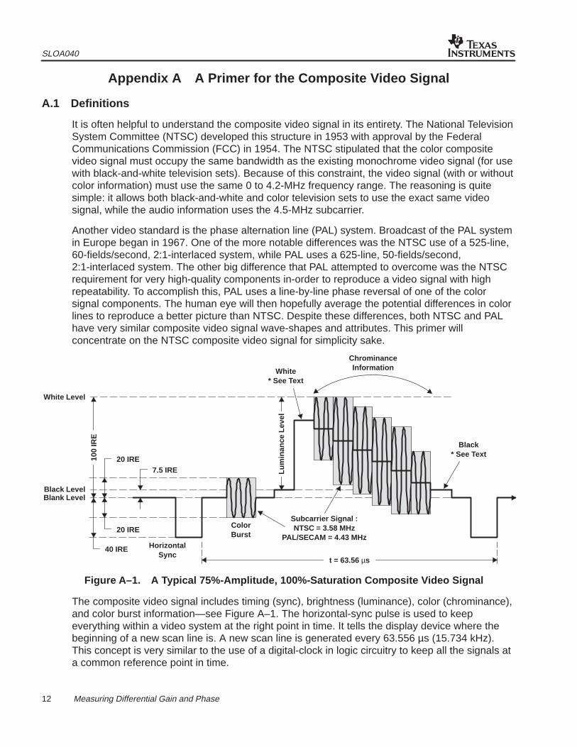
Figure A–1. A Typical 75%-Amplitude, 100%-Saturation Composite Video Signal

The composite video signal includes timing (sync), brightness (luminance), color (chrominance),and color burst information—see Figure A–1. The horizontal-sync pulse is used to keepeverything within a video system at the right point in time. It tells the display device where thebeginning of a new scan line is. A new scan line is generated every 63.556 µs (15.734 kHz).This concept is very similar to the use of a digital-clock in logic circuitry to keep all the signals ata common reference point in time.

SLOA040


The brightness information is the luminance portion of the composite video signal. Because thehuman eye is more sensitive to brightness variations, the entire bandwidth (0 to 4.2 MHz) isallocated to reproducing the luminance information. The brighter (or whiter) the picture is, thehigher the video-signal amplitude. Video signals use the arbitrary IRE unit for amplitudemeasurements. A pure-white signal corresponds to a 100-IRE level, while the blanking level,which is blacker than black, corresponds to a 0-IRE level. Sometimes it is required to relate theIRE measurement to volts. The NTSC standard states that 100 IRE should correspond to 714 ±7mV, while the PAL standard establishes it at 700 ± 7 mV. This difference is generally ignored tokeep things simple. The most common conversion used is 1 VPP = 140 IRE, or 1 IRE = 7.14 mV.

The color information (chrominance) is encoded within a subcarrier frequency. For mostsystems, this subcarrier frequency is 3.579545 MHz ±10 Hz for the NTSC standard, and4.43361875 MHz ±5 Hz for the PAL standard. There are two parts to the color information: hueand saturation. Hue is technically the wavelength of a color. It can be thought of as the basecolor within the whole color spectrum. The other part to the color information, saturation,determines the intensity of a specific color. For example, the color red may look very dull withvery little saturation, or it may look deep red with very high saturation. The fact that its base coloris red still remains.

If the luminance portion takes up the full 0 to 4.2 MHz band, then what is the bandwidth for thecolor portion? To help answer this, we need to know how the color subcarrier came to be. Thefirst thing to realize is that the NTSC color subcarrier was chosen for a reason. The audio carrieris at 4.5 MHz. The 286th harmonic of the already existing 15.75-kHz monochromehorizontal-scan frequency is about 4.5 MHz. In the color system, this 4.5-MHz frequency isdivided by 286 to obtain the new horizontal-scan frequency of 15.743 kHz. This result is withinthe deviation limit originally set by the NTSC monochrome standards. The luminance informationis then based on this 15.743-kHz separation. To minimize the visibility of the color subcarrier, itsfrequency is chosen to be an odd multiple of one-half the horizontal scan rate. This thenperforms frequency interleaving (see Figure A–2). The color information is also allowed to havea 0.6 MHz side band. This leaves a maximum upper frequency of 4.2 MHz (from the luminancebandwidth limit)—0.6 MHz = 3.6 MHz. It was found that the 455th harmonic (5 × 7 × 13 = 455) ofone-half the color scan rate (15.743 kHz/2) is equal to 3.579545 MHz.

SLOA040


15.734 kHz

Sig

nal S

tren

gth

Frequency – MHz

Y

0 1 2 2.28 43.58 4.23

MagnifiedView

I, Q(U, V)

ChrominanceEnergy Density

LuminanceEnergy Density

Y Y

227 228227.5

I, Q(U, V)

227.5 =3.579545 MHz

Figure A–2. Frequency Interleaving Spectrum

Let’s now find the color information bandwidth. As stated earlier, the color information is alloweda 0.6-MHz side band. All three color components are allowed to use the entire bandwidth forlarge objects. For medium-sized objects a 1.3-MHz bandwidth is allowed, but is generally limitedto two colors. The choice of these colors is discussed further in this document. A filter is placedat 4.2 MHz to insure that the 1.3-MHz upper-side band does not interfere with the sound carrier.Most consumer-grade equipment uses only the 0.6-MHz side bands, while studio qualityequipment generally use the fully-allotted spectrum (see Figure A–3).

Sig

nal S

tren

gth

Frequency – MHz

0 1 32.282.282 4 4.23.58

LuminanceY

Subcarrier

I IQ

IQ S

igna

l Str

engt

h

Frequency – MHz

0 1 32.282.282 4 4.23.58

LuminanceY

Subcarrier

UV

UV

Figure A–3. NTSC Composite Video Frequency Spectrum

The last part to a composite-video signal is the color burst. The color burst tells the video circuitcolor decoder how to decode the color information contained within the following line of video. Itensures that the colors displayed match those of the original source material. This isaccomplished by sending 8 to 11 subcarrier cycles. These cycles are sent in phase with thesubcarrier used to record the original picture. The receiving circuitry can then lock this frequencyand phase for its own subcarrier oscillator. Because the color burst is only transmitted with colormaterial, the decoding circuitry can tell if the composite video signal is black-and-white or colorand adjust its compensation accordingly.

SLOA040


A.2 Creating the Composite Video Signal

Now that we know what the composite-video signal components are, let us see how the pictureinformation is encoded. If the signal is purely monochrome, the video signal only has theluminance component and no color subcarrier component. This is quite straightforward andshould be easy to see how a monochrome signal is encoded. The tricky part is getting the hueand saturation components into the composite video signal.

The first and most important part of the composite video signal is the luminance information. Theluminance (or brightness) is derived from the gamma-corrected red (R’), green (G’), and blue(B’) signals. Gamma correction takes into account the fact that the intensity of the display device(typically a cathode-ray tube—CRT) is proportional to the signal voltage raised to some power(typically 2.2 to 2.6). As a result of this relationship, high-intensity images are even brighter, andlow-intensity ones become even darker. To correct for this, the red, green, and blue (RGB)transmitted signal levels are reduced by a factor of 1/2.2 = 0.45. An advantage of this correctionis an increase in the signal-to-noise ratio during transmission. For clarification purposes, thecomponent signals are shown below.

RDISPLAYED RSIGNAL2.2

and RTRANSMIT RSIGNAL0.45

R

GDISPLAYED GSIGNAL2.2

and GTRANSMIT GSIGNAL0.45

G

BDISPLAYED BSIGNAL2.2

and BTRANSMIT BSIGNAL0.45

B

When talking about transmitted color components, the gamma-corrected color components(R’G’B’) are used for all of the signal levels in the composite-video signal.

The luminance information (or brightness) is formed by the basic R’G’B’ color combination.When these signals are set to zero, the luminance information portrays a black color. When thethree signals are set to 100% level, the luminance information portrays a white color. It thenbecomes clear that every other color falling between black and white can be encoded. Thisallows a black-and-white television set to reproduce an image created from a color source.

The formula for luminance is:

Y (luminance) 0.299 R 0.587 G 0.114 B

We can also see that color weighting is used for the transmission of each color. This is becausethe human eye is more sensitive to green than to red, and more sensitive to red than to blue. Itmakes sense to have the dominant portion of the signal be the color that our eyes are mostsensitive to. This naturally brings us to how the rest of the color information is encoded.

The hue and saturation information is encoded by using a color-difference formula. This is doneby running the luminance (Y) information through an inverter to obtain –Y. This signal is thenadded to the R’ and B’ color signals to get:

R Y 0.701 R 0.587 G 0.114 B

B Y 0.299 R 0.587 G 0.886 B

(2)

(3)

(4)

(5)

(6)

(7)

SLOA040


But what about the third color-difference signal, G’ – Y? Because the luminance signalincorporates the G’ component, sending the G’ – Y portion is not required. At the receiver side,to extract the original R’G’B’ components, we simply do the following:

(R Y) Y R

(B Y) Y B

(Y – R – B) × 1.704 G

or

Y 0.510 (R Y) 0.194 (B Y) G

Equations (5) through (11) show that it is only necessary to send two parts of the R’G’B’ signalinstead of all three. To simplify equations (6) and (7) even further, the color-differencecomponents U and V were created

U 0.492 (B Y)

V 0.877 (R Y)

To get back to the R’G’B’ discrete signals using the U and V methodology, use the following:

R Y 1.140 V

B Y 2.032 U

G Y 0.394 U 0.581 V

It is also common to see the I and Q components used in place of U and V. This is donebecause when medium-size objects are displayed on a screen, the eye is more sensitive tocertain colors. These colors are the bluish-greens and the reddish-oranges. Medium-size objectsuse the full 1.3-MHz lower-side band (LSB) of the subcarrier energy distribution (see FigureA–3). However, the Q signal is filtered to show only the 0.6-MHz LSB portion. So, formedium-size objects, the Q-signal amplitude is reduced to zero. On the other hand, the I signalis allowed to use the full 1.3-MHz LSB spectrum. When only the I signal is used, just thesensitive color range from the bluish-greens to the reddish-oranges is shown (see Figure A–4).Hence, the I and Q scheme was created to exploit the sensitivity of the human eye beyond whatthe U and V formulas provide.

I 0.596 R 0.275 G 0.321 B

V cos 33°U sin 33°

0.736 (R Y) 0.268 (B Y)

and

Q 0.212 R 0.523 G 0.311 B

V sin 33°U cos 33°

0.478 (R Y) 0.413 (B Y)

(8)

(9)

(10)

(11)

(12)

(13)

(14)

(15)

(16)

(17)

(18)

(19)

(20)

(21)

(22)

SLOA040


To get back to the R’G’B’ discrete signals using the I and Q methodology, we perform thefollowing:

R Y 0.956 I 0.620 Q

B Y 1.108 I 1.705 Q

G Y 0.272 I 0.647 Q

The I and Q (or U and V) signals are then used to modulate the subcarrier frequency. Using aphase-quadrature mixing scheme produces the chrominance signal. Modulating one signal at asine phase and adding the other signal, which is modulated with a cosine phase, results in thechrominance-signal formulas:

Chrominance signal Q sin (t 33°) I cos (t 33°)

or

Chrominance signal U sin t V cos t

Where ω = 2 π FSUBCARRIER

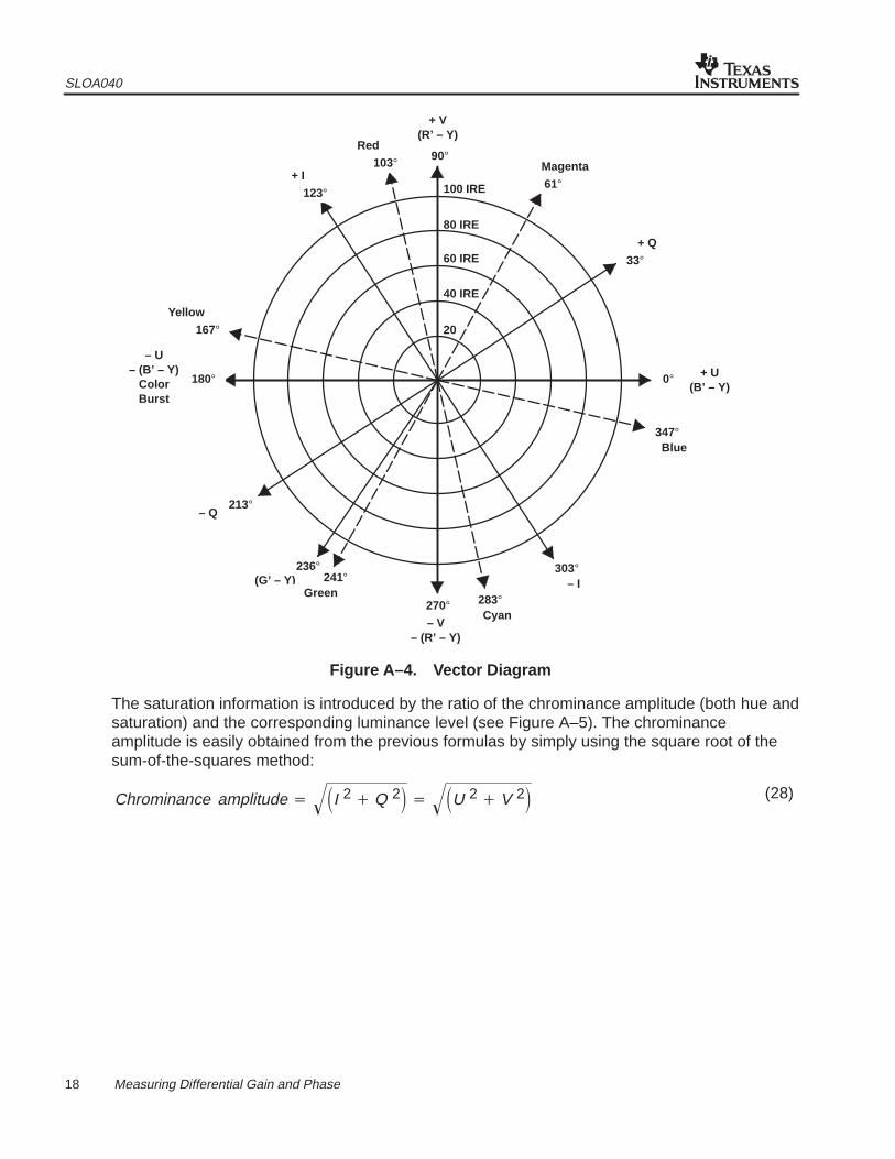
The hue information is introduced into the signal by a phase shift relative to the subcarrierreference signal, as shown in Equations 26 and 27. For example, the color red is at aphase-shift of 103° relative to the sub-carrier, green is at 241° relative to the subcarrier, and blueis 347° relative to the subcarrier. By setting the correct phase relative to the subcarrier referencesignal, any color can be realized on a vector diagram (see Figure A–4). The only thing left toproduce the proper color is to find the proper color saturation.

(23)

(24)

(25)

(26)

(27)

SLOA040


90°

+ V(R’ – Y)

61°Magenta

33°+ Q

270°– V

– (R’ – Y)

0° + U(B’ – Y)

180°

– U– (B’ – Y)

ColorBurst

123°+ I

103°Red

167°Yellow

213°– Q

236°(G’ – Y) 241°

Green283°Cyan

303°– I

347°Blue

100 IRE

80 IRE

60 IRE

40 IRE

20

Figure A–4. Vector Diagram

The saturation information is introduced by the ratio of the chrominance amplitude (both hue andsaturation) and the corresponding luminance level (see Figure A–5). The chrominanceamplitude is easily obtained from the previous formulas by simply using the square root of thesum-of-the-squares method:

Chrominance amplitude I 2 Q 2 U 2 V 2 (28)

SLOA040


Col

or S

atur

atio

n Le

vel

HUE = Phase Difference From Subcarrier(HUE = Color)

(See Vector Diagram)

(Rat

io o

f Sub

carr

ier

Sig

nal

Am

plitu

de to

Lum

inan

ce L

evel

)Luminance Level(Luminance = Brightness)

Figure A–5. Chrominance Signal Components

This chrominance signal is then added to the luminance (Y) signal to create the composite-videosignal shown in Figure A–1. The additional portions to the composite-video signal are added bydifferent means generally not related to the encoding algorithm. These portions include, but arenot limited to, the horizontal sync, color burst, and blanking signals. The exact formula for thecomposite-video signal is:

Chrominance NTSC YQ sin (t 33°) I cos (t 33°)

or

Chrominance NTSC YU sin t V cos t

It may be helpful to note that if no color is encoded, there will be no subcarrier modulation withinthe composite-video signal. This can be seen in the example composite-video line shown inFigure A–1. The first section within the video information portion shows a flat-luminance line,coupled with no subcarrier amplitude and a high IRE level. This will produce the color white on ascreen. Additionally, the last portion shown within the video information with a 7.5 IRE level willshow the color black on the screen.

To see all of these concepts and equations in action, let us look at the standard test patternshown in A of Figure A–6. This represents a single horizontal line being scanned from left toright across the screen. It consists of every combination of the three basic colors; red, green,and blue. B, C, and D of Figure A–6 show the relative saturation levels of the three basic colorsusing 100% as the maximum saturation level. The luminance formula of Equation 5 using thesaturation levels shown results in E of Figure A–6. The next step is to create the I and Q signalsusing Equations 17 and 20, as shown in F and G of Figure A–6. Using Equations 26 and 27results in the 3.58-MHz modulated-subcarrier waveform shown in H and I of Figure A–6. Next,combine the chrominance signal (H and I) with the luminance signal (E). Before the finalcomposite waveform is produced, we should take into account that the black level is at 7.5 IREand not at 0 IRE as mandated by the NTSC. A small correction factor has to be added toaccount for the 92.5 IRE full scale instead of a 100 IRE full scale. The resulting correctedcomposite waveform is shown in J of Figure A–6.

(29)

(30)

SLOA040


Whi

te

Yel

low

Cya

n

Gre

en

Mag

enta

Red

Blu

e

Bla

ck

100

0

%Red

ComponentB

A

100

0

%Green

ComponentC

100

0

%Blue

ComponentD

100

0

IREE

100 8970 59

41 3011 0

Y – LuminanceLevel

+

–

IREF 032 28

60

0

–32–28–60

I Signal

+

–

IREG 0Q Signal

5221 31

0

–31 –21–52

+

–

IREH 0 ChrominanceLevel

–44

4463 59

4463

0

–59 –44–63–63

360

0

Deg.I0

ChrominancePhase

167284 241

61 104

347

0

Horizontal Scan Line

48

131

100

0

IREJCorrectedComposite

Signal

100116

100 94

59

14 7–9

–23

7.5

Figure A–6. The Construction of an NTSC Composite Video Signal

SLOA040


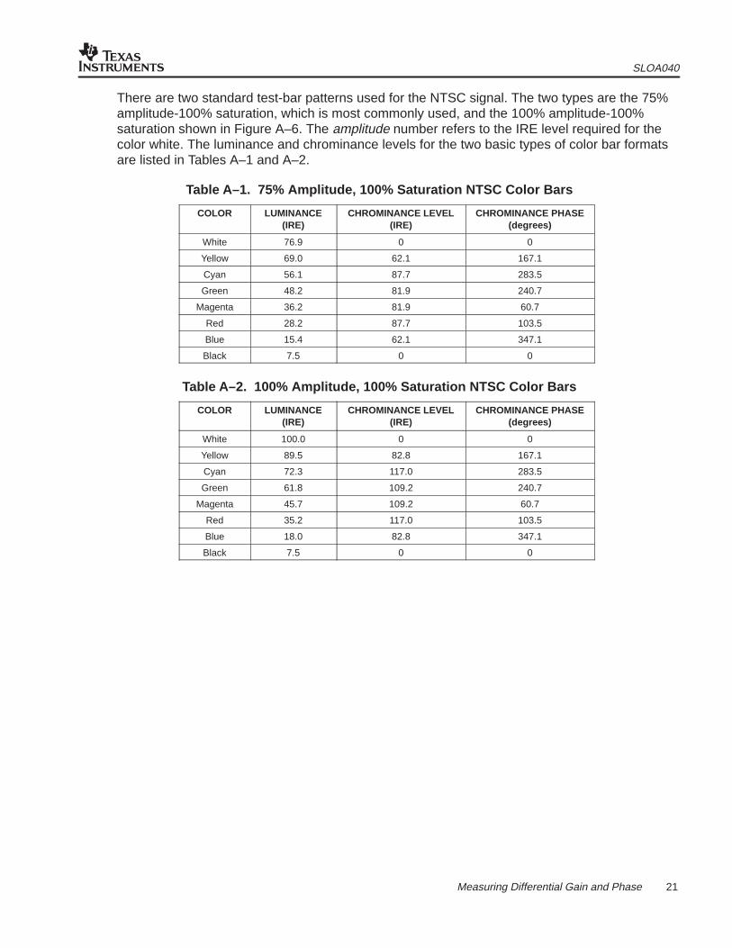
There are two standard test-bar patterns used for the NTSC signal. The two types are the 75%amplitude-100% saturation, which is most commonly used, and the 100% amplitude-100%saturation shown in Figure A–6. The amplitude number refers to the IRE level required for thecolor white. The luminance and chrominance levels for the two basic types of color bar formatsare listed in Tables A–1 and A–2.

Table A–1. 75% Amplitude, 100% Saturation NTSC Color Bars

COLOR LUMINANCE(IRE)

CHROMINANCE LEVEL(IRE)

CHROMINANCE PHASE(degrees)

White 76.9 0 0

Yellow 69.0 62.1 167.1

Cyan 56.1 87.7 283.5

Green 48.2 81.9 240.7

Magenta 36.2 81.9 60.7

Red 28.2 87.7 103.5

Blue 15.4 62.1 347.1

Black 7.5 0 0

Table A–2. 100% Amplitude, 100% Saturation NTSC Color Bars

COLOR LUMINANCE(IRE)

CHROMINANCE LEVEL(IRE)

CHROMINANCE PHASE(degrees)

White 100.0 0 0

Yellow 89.5 82.8 167.1

Cyan 72.3 117.0 283.5

Green 61.8 109.2 240.7

Magenta 45.7 109.2 60.7

Red 35.2 117.0 103.5

Blue 18.0 82.8 347.1

Black 7.5 0 0

IMPORTANT NOTICE

Texas Instruments and its subsidiaries (TI) reserve the right to make changes to their products or to discontinueany product or service without notice, and advise customers to obtain the latest version of relevant informationto verify, before placing orders, that information being relied on is current and complete. All products are soldsubject to the terms and conditions of sale supplied at the time of order acknowledgement, including thosepertaining to warranty, patent infringement, and limitation of liability.

TI warrants performance of its semiconductor products to the specifications applicable at the time of sale inaccordance with TI’s standard warranty. Testing and other quality control techniques are utilized to the extentTI deems necessary to support this warranty. Specific testing of all parameters of each device is not necessarilyperformed, except those mandated by government requirements.

CERTAIN APPLICATIONS USING SEMICONDUCTOR PRODUCTS MAY INVOLVE POTENTIAL RISKS OFDEATH, PERSONAL INJURY, OR SEVERE PROPERTY OR ENVIRONMENTAL DAMAGE (“CRITICALAPPLICATIONS”). TI SEMICONDUCTOR PRODUCTS ARE NOT DESIGNED, AUTHORIZED, ORWARRANTED TO BE SUITABLE FOR USE IN LIFE-SUPPORT DEVICES OR SYSTEMS OR OTHERCRITICAL APPLICATIONS. INCLUSION OF TI PRODUCTS IN SUCH APPLICATIONS IS UNDERSTOOD TOBE FULLY AT THE CUSTOMER’S RISK.

In order to minimize risks associated with the customer’s applications, adequate design and operatingsafeguards must be provided by the customer to minimize inherent or procedural hazards.

TI assumes no liability for applications assistance or customer product design. TI does not warrant or representthat any license, either express or implied, is granted under any patent right, copyright, mask work right, or otherintellectual property right of TI covering or relating to any combination, machine, or process in which suchsemiconductor products or services might be or are used. TI’s publication of information regarding any thirdparty’s products or services does not constitute TI’s approval, warranty or endorsement thereof.

Copyright 1999, Texas Instruments Incorporated

Measuring Differential Gain and Phase - Texas … Differential Gain and Phase Randy Stephens Mixed...

Documents

Transcript of Measuring Differential Gain and Phase - Texas … Differential Gain and Phase Randy Stephens Mixed...