MEASURING CONSUMER AND COMPETITIVE IMPACT WITH

ELASTICITY DECOMPOSITIONS

Thomas J. Steenburgh1

1 Thomas J. Steenburgh is an Assistant Professor at the Harvard Business School. He would like to thank David E. Bell, Sunil Gupta, and Harald van Heerde for comments and suggestions that greatly improved the quality of this manuscript. He also gratefully acknowledges the support of his late thesis advisor, Dick Wittink. The author, of course, is solely responsible for any errors. Address: Harvard Business School, Soldiers Field, Boston, MA 02163 Phone: 617-495-6056 Fax: 617-496-5853 E-mail: tsteenburgh@hbs.edu

MEASURING CONSUMER AND COMPETITIVE IMPACT WITH

ELASTICITY DECOMPOSITIONS

In this article, I discuss three methods of decomposing the elasticity of own-good

demand. One of the methods, the decision-based decomposition (Gupta, 1988), is useful

in determining the influence of changes in consumers’ decisions on the growth in own-

good demand. The other two methods, the unit-based decomposition (van Heerde et al.,

2003) and the share-based decomposition (Berndt et al., 1997), are useful in determining

whether the growth in own-good demand has been stolen from competing goods.

The objective of this article is to provide a clear and accurate method that

attributes the growth in own-good demand to changes in: (1) consumers’ decisions, (2)

competitive demand, and (3) competitive market share. I will accomplish this by settling

some confusion about what the decision- and share-based decompositions mean, by

discussing how each of the decompositions relate to the others, and by discussing the

research questions that each of the decompositions can answer.

1

I. Introduction

Three methods of decomposing the elasticity of demand have been used to study

whether marketing actions expand the market or steal business from rival firms. These

decompositions, when applied to the same problem, produce seemingly contradictory

results. One method, for example, may suggest that all of the demand created by an

incremental advertising investment would be generated by market expansion while

another suggests the same increase would be stolen from rival firms. I will explain why

these apparently contradictory results actually are complementary and provide a more

comprehensive understanding of the investment’s impact.

Consider the following example. Suppose two firms are competing in a market.

Firm A is considering whether to increase its advertising investments by a small amount.

The unit sales and market shares that would be earned by the firms at the two investment

levels are summarized in Table One. Firm A would like to know whether the growth in

its demand comes at the expense of Firm B.

< Insert Table One >

Several methods have been developed to answer this question. The crucial

difference among them lies in how the researchers measure stolen business. Some authors

measure stolen business by the decrease in demand for competing goods (van Heerde et

al., 2003; van Heerde et al., 2004). I will refer to these methods as unit-based

decompositions. In our example, these authors would claim that none of the growth in

Firm A’s demand would come at the expense of Firm B because Firm B’s demand would

not be affected by the advertising investment. This is a reasonable point of view to take.

Other authors measure stolen business by the decrease in market share of

2

competing goods (Berndt et al., 1995; Berndt et al., 1997; Rosenthal et al., 2003). I will

refer to these methods as share-based decompositions. In our example, these authors

would claim that some of the growth in Firm A’s demand would come at the expense of

Firm B because Firm B’s market share would drop by 1.3 percentage points due to the

advertising investment. This too is a reasonable point of view to take.

Despite appearing to offer very similar measures of stolen business, the unit- and

share-based methods can produce strikingly different results. In our example, the unit-

based measure suggests that none of the growth in Firm A’s demand would come at the

expense of Firm B, but the share-based measure suggests that two-thirds of it would.

Firm B would need to earn 1,020 units in the expanded market in order to maintain its

original market share. Since it earns only 1,000 units, the share-based measure classifies

20 units of the 30 unit increase as being stolen from it.

Not only do these decompositions give very different impressions of what is

happening in the marketplace, the share-based method has not been fully understood.

Berndt et al. (1997) write:

We distinguish between two types of marketing: (1) that which concentrates on bringing

new customers into the market (“[market]-expanding” advertising), and (2) that which

concentrates on competing for market shares from these consumers (“rivalrous”

advertising).

This interpretation is misleading. Share-based decompositions classify only a portion of

the market expansion as being primary (or non-rivalrous) demand. In our example, the

share-based decomposition classifies only 10 units of the 30 unit increase in market

demand as primary. By contrast, the unit-based measure defines primary demand to be

equivalent to the market expansion, the full 30 unit increase.

3

A third set of authors study a marketing action’s impact from an entirely different

perspective. They measure the influence of changes in the consumers’ decisions on the

growth in own-good demand (Gupta, 1988; Chiang, 1991; Chintagunta, 1993; Bucklin et

al., 1999; and Bell et al., 1999). I will refer to these as decision-based decompositions.2

These decompositions, contrary to some suggestions otherwise, are insufficient to

determine a marketing investment’s competitive impact because they measure changes

only in own-good demand, not in competitive demand. Nevertheless, I will show how to

extend a decision-based analysis to competing goods by decomposing the elasticity of

cross-good demand.

The objective of this article is to provide a clear and accurate method that

attributes the growth in own-good demand to changes in: (1) consumers’ decisions, (2)

competitive demand, and (3) competitive market share. I will accomplish this by settling

some confusion about what the decision- and share-based decompositions mean, by

discussing how each of the decompositions relates to the others, and by discussing the

research questions that each of the decompositions can answer. From the unit-based

decomposition, a brand manager can learn whether the growth in own-good demand is

due to stolen units. From the share-based decomposition, a manager can learn whether it

is due to stolen market share. From the decision-based decomposition, a manager can

learn which changes in consumer behavior lead to the growth in demand. Used together,

these methods provide a comprehensive understand of a marketing investment’s impact.

The remainder of the paper is organized as follows. In section two, I derive the

relationship between the unit- and share-based decompositions. Contrasting the two

2 I will show that any of the decompositions, even the unit-based one, can be derived from the elasticity of demand. Therefore, I will eschew using the term elasticity decomposition to distinguish the decision-based decomposition from the others.

4

decompositions clarifies the perspective that each method offers and coerces a more

precise interpretation of the share-based method. I illustrate the difference between the

methods using an example based on the empirical results of Berndt et al. (1997). In

section three, I decompose the elasticity of cross-good demand to isolate the impact of

each consumer decision on competitive demand. This analysis resolves the discrepancies

in the coffee example of van Heerde et al. (2003) and clarifies the meaning of decision-

based decompositions. In section four, I derive the relationships between the decision-

based and the unit- and share-based decompositions using the previous cross-good

analysis. This allows me to construct matrices that fully account for how a marketing

action affects both consumers’ decisions and the demand for and market-share of

competing goods. I illustrate the unified decompositions by returning to the coffee

example and discuss a paradox that can arise when the own-good market share is low. I

conclude in section five. All of the decompositions that will be discussed measure an

investment’s contemporaneous effects.

2. Decompositions that Measure Competitive Impact

Let’s begin by comparing the unit- and share-based approaches to studying a

marketing action’s competitive impact. Both methods attribute the growth in own-good

demand to rivalrous and non-rivalrous sources. The unit-based method measures stolen

business by the decrease in demand for competing goods whereas the share-based method

measures stolen business by the decrease in their market share. Neither method requires a

model of the consumers’ decision-making process in order to make this judgment. I will

show that both decompositions accurately depict how a marketing action would affect

competing goods and will explain how to interpret differences in their results.

5

Let’s begin with some notation. Let jq represent the demand for good j,

1

J

j kkk j

Q q−=≠

=∑ represent the demand for competing goods (competitive demand), and

1

J

all kk

Q q=

= ∑ represent the demand for all goods in the market (market demand).

Similarly, let js represent the market share of good j and 1

J

j kkk j

S s−=≠

= ∑ represent the share

of competing goods. Let jm be a marketing instrument for good j. The elasticities of

demand are ,j j

j jq m

j j

q mm q

η∂

= ⋅∂

, ,j j

j jQ m

j j

Q mm Q

η−

−

−

∂= ⋅∂

, and ,all j

jallQ m

j all

mQm Q

η ∂= ⋅∂

and of share

are ,j j

j js m

j j

s mm s

η∂

= ⋅∂

and ,j j

j jS m

j j

S mm S

η−

−

−

∂= ⋅∂

.

2.1 Unit-Based Decompositions

Unit-based decompositions measure stolen business by the decrease in demand

for competing goods. These decompositions are derived from the identity

j all jq Q Q−= − . (1)

Demand for the target good is expressed as the difference between demand for all goods

in the market and demand for competing goods.

The impact of an incremental marketing investment is quantified by taking

derivatives, such that

j jall

j j j

q QQm m m

−∂ ∂∂= −

∂ ∂ ∂. (2)

This equation attributes the growth in own-good demand to two sources. The non-

6

rivalrous source is measured by the increase in market demand, all jQ m∂ ∂ . The rivalrous

source is measured by the decrease in demand for competing goods, j jQ m−∂ ∂ .

Figure One provides a geometric depiction of the unit-based decomposition. As

the result of an incremental marketing investment, the market expands from A to A′ and

the demand for competing goods contracts from B to B′ . Line segment AB represents

the demand for good j prior to the incremental marketing investment and line segment

A B′ ′ represents demand afterwards. Demand for good j grows by A C′ + DB′ units. Of

the growth, A C′ units are generated by market expansion and DB′ units are stolen from

competing goods. Demand for competing goods decreases by DB′ units. For small

j jm mδ ′= − , the quantities represented by the line segments are all

j

QA Cm

δ∂′ = ⋅∂

and

j

j

QDB

mδ−∂

′ = − ⋅∂

.

< Insert Figure One >

Unit-based decompositions can be transformed from derivatives into elasticities

by multiplying all terms by j jm q . This transformation results in

( ) ( ), , ,j j all j j jq m all j Q m j j Q mQ q Q qη η η−−= ⋅ − ⋅ . (3)

The leading term all jQ q simply scales the change in market demand from being

measured relative to the level of market demand to being measured relative to the level of

demand for good j. Similarly, the leading term j jQ q− scales the change in demand for

competing goods from being measured relative to the level of demand for competing

goods to being measured relative to the level of demand for good j.

7

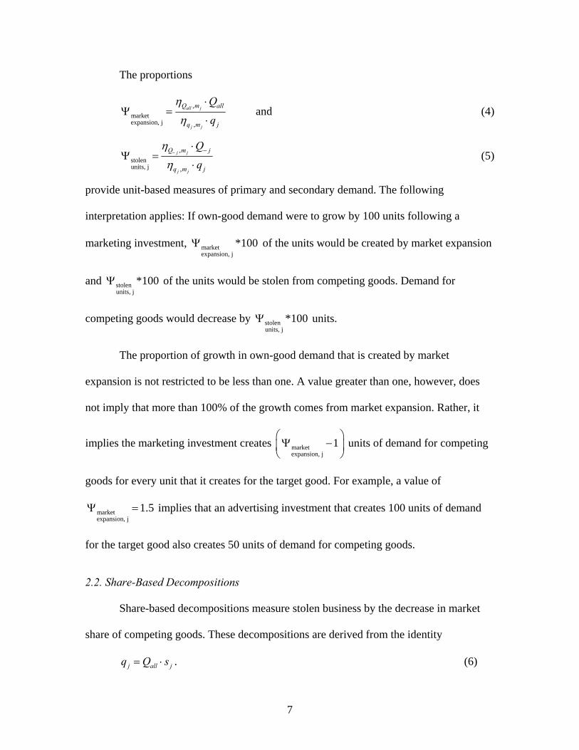
The proportions

,marketexpansion, j ,

all j

j j

Q m all

q m j

Q

q

η

η

⋅Ψ =

⋅ and (4)

,stolenunits, j ,

j j

j j

Q m j

q m j

Q

q

η

η− −⋅

Ψ =⋅

(5)

provide unit-based measures of primary and secondary demand. The following

interpretation applies: If own-good demand were to grow by 100 units following a

marketing investment, marketexpansion, j

*100Ψ of the units would be created by market expansion

and stolenunits, j

*100Ψ of the units would be stolen from competing goods. Demand for

competing goods would decrease by stolenunits, j

*100Ψ units.

The proportion of growth in own-good demand that is created by market

expansion is not restricted to be less than one. A value greater than one, however, does

not imply that more than 100% of the growth comes from market expansion. Rather, it

implies the marketing investment creates marketexpansion, j

1⎛ ⎞Ψ −⎜ ⎟⎝ ⎠

units of demand for competing

goods for every unit that it creates for the target good. For example, a value of

marketexpansion, j

1.5Ψ = implies that an advertising investment that creates 100 units of demand

for the target good also creates 50 units of demand for competing goods.

2.2. Share-Based Decompositions

Share-based decompositions measure stolen business by the decrease in market

share of competing goods. These decompositions are derived from the identity

j all jq Q s= ⋅ . (6)

8

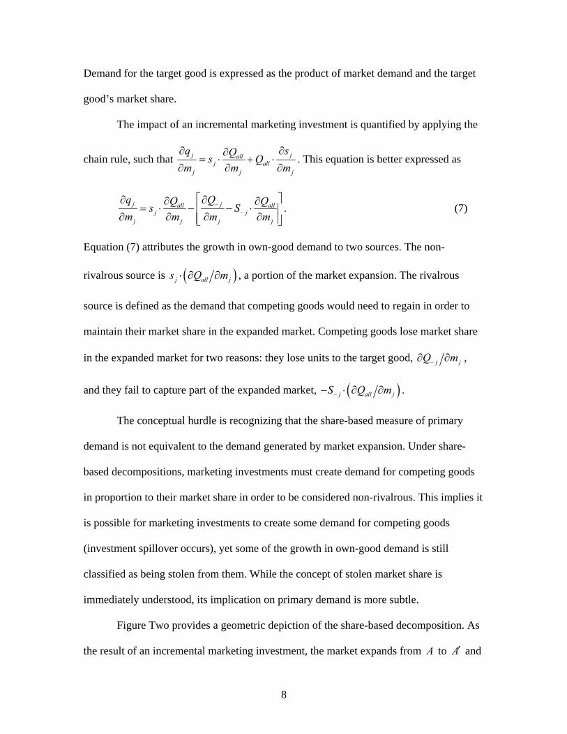
Demand for the target good is expressed as the product of market demand and the target

good’s market share.

The impact of an incremental marketing investment is quantified by applying the

chain rule, such that j jallj all

j j j

q sQs Qm m m∂ ∂∂

= ⋅ + ⋅∂ ∂ ∂

. This equation is better expressed as

j jall allj j

j j j j

q QQ Qs Sm m m m

−−

⎡ ⎤∂ ∂∂ ∂= ⋅ − − ⋅⎢ ⎥

∂ ∂ ∂ ∂⎢ ⎥⎣ ⎦. (7)

Equation (7) attributes the growth in own-good demand to two sources. The non-

rivalrous source is ( )j all js Q m⋅ ∂ ∂ , a portion of the market expansion. The rivalrous

source is defined as the demand that competing goods would need to regain in order to

maintain their market share in the expanded market. Competing goods lose market share

in the expanded market for two reasons: they lose units to the target good, j jQ m−∂ ∂ ,

and they fail to capture part of the expanded market, ( )j all jS Q m−− ⋅ ∂ ∂ .

The conceptual hurdle is recognizing that the share-based measure of primary

demand is not equivalent to the demand generated by market expansion. Under share-

based decompositions, marketing investments must create demand for competing goods

in proportion to their market share in order to be considered non-rivalrous. This implies it

is possible for marketing investments to create some demand for competing goods

(investment spillover occurs), yet some of the growth in own-good demand is still

classified as being stolen from them. While the concept of stolen market share is

immediately understood, its implication on primary demand is more subtle.

Figure Two provides a geometric depiction of the share-based decomposition. As

the result of an incremental marketing investment, the market expands from A to A′ and

9

demand for competing goods contracts from B to B′ . Line segment AB represents

demand for good j prior to the incremental investment and line segment A B′ ′ represents

it afterwards. Demand for good j grows by A EC′ + DB′ units. For market shares to be

preserved, the ratio of A E′ to A C′ is equivalent to the ratio of AB to AF . Of the

growth in demand for good j, A E′ units are defined as non-rivalrous and EC + DB′ units

are generated by stealing share from competing goods. Demand for competing goods

decreases by DB′ units. For small j jm mδ ′= − , the quantities represented by the line

segments are allj

j

QA E sm

δ∂′ = ⋅ ⋅∂

, allj

j

QEC Sm

δ−∂

= ⋅ ⋅∂

, and j

j

QDB

mδ−∂

′ = − ⋅∂

.

< Insert Figure Two >

Expressed in terms of elasticities, the share-based decomposition is

( ) ( ), , , ,j j all j j j all jq m j Q m j j Q m j all j Q ms Q q S Q qη η η η−− −

⎡ ⎤= ⋅ − ⋅ − ⋅ ⋅⎣ ⎦ . (8)

The proportions

( ),

share-preservingmarket expansion, j ,

all j

j j

j Q m all

q m j

s Q

q

η

η

⋅ ⋅Θ =

⋅ and (9)

( ) ( ), ,

stolenshare, j ,

j j all j

j j

Q m j j Q m all

q m j

Q S Q

q

η η

η− − −− ⋅ + ⋅ ⋅

Θ =⋅

(10)

provide share-based measures of primary and secondary demand. These measures are

related to those of the unit-based decomposition through the expressions

share-preserving market market expansion, j expansion, j

jsΘ = ⋅Ψ and (11)

stolen stolen market share, j units, j expansion, j

jS−Θ = Ψ + ⋅Ψ . (12)

This relationship should be expected. Both decompositions attribute the growth in own-

10

good demand to changes in demand for competing goods. The share-based

decomposition, however, attributes the demand competing goods would earn in an

expanded market if they kept their market share, market expansion, j

jS− ⋅Ψ , to the rivalrous source.

The unit- and share-based decompositions are simply different measures of competitive

impact, and one can be recovered from the other without consideration of the consumers’

decision-making process. All information needed to determine these decompositions is

contained in the elasticities of own- and cross-good demand.

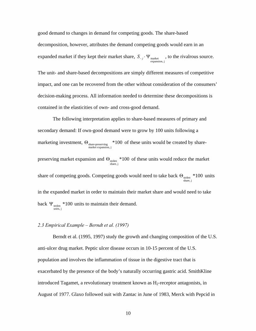
The following interpretation applies to share-based measures of primary and

secondary demand: If own-good demand were to grow by 100 units following a

marketing investment, share-preservingmarket expansion, j

*100Θ of these units would be created by share-

preserving market expansion and stolenshare, j

*100Θ of these units would reduce the market

share of competing goods. Competing goods would need to take back stolenshare, j

*100Θ units

in the expanded market in order to maintain their market share and would need to take

back stolenunits, j

*100Ψ units to maintain their demand.

2.3 Empirical Example – Berndt et al. (1997)

Berndt et al. (1995, 1997) study the growth and changing composition of the U.S.

anti-ulcer drug market. Peptic ulcer disease occurs in 10-15 percent of the U.S.

population and involves the inflammation of tissue in the digestive tract that is

exacerbated by the presence of the body’s naturally occurring gastric acid. SmithKline

introduced Tagamet, a revolutionary treatment known as H2-receptor antagonists, in

August of 1977. Glaxo followed suit with Zantac in June of 1983, Merck with Pepcid in

11

October of 1986, and Lilly with Axid in April of 1988.

Berndt et al. (1995, 1997) estimate a system of two equations to describe

consumer demand for these drugs. They specify a log-linear demand equation to describe

the relationship between the market (industry) demand and the firms’ marketing

investments. They also specify a relative demand equation to describe the relationship

between the firms’ relative market shares and the relative investments made in support of

their drugs. I will use Berndt et al.’s (1997) estimates from the two-product market that

contains Tagamet and Zantac.3 The elasticity of market demand is -0.268 for a change in

the price of Tagamet and -0.804 for a change in the price of Zantac. The own-good

elasticity of demand is -1.154 for Tagamet and is -1.690 for Zantac.

The share- and unit-based measures of primary and secondary demand are given

in Table Two. The results of these methods provide very different impressions of whether

price cuts steal business. Regardless of whether Tagamet or Zantac cuts its price, the unit-

based measure suggests most of the growth in own-good demand comes from primary

demand (92.9% for Tagamet and 63.4% for Zantac) whereas the share-based measure

suggests most of the growth comes from secondary demand (76.8% for Tagamet and

52.4% for Zantac).

< Insert Table Two >

The decompositions, of course, are describing the competitive impact of the same

price cut and should be interpreted as follows: A 1% decrease in Tagamet’s price would

yield a 1.154% increase in its demand. From the unit-based decomposition, we can say

3 Parameter estimates for the market-level equation are found in column 2 of Table 7.1 on p. 301 and estimates for the market-share equation are found in column 4 of Table 7.2 on p. 307 of Berndt et al. (1997).

12

92.9% of the growth in Tagamet’s demand would come from market expansion and 7.1%

would be stolen from Zantac. This implies Zantac would have to take back 0.071 *

0.01154 * Tagametq units from Tagamet in order to maintain its demand. From the share-

based decomposition, we can say Zantac would need to take back 76.8% of the growth in

demand for Tagamet, which amounts to 0.768 * 0.01154 * Tagametq units, in order to

maintain its market share in the expanded market. A similar analysis would apply to the

growth in demand for Zantac if it were to cut its price.

The unit- and share-based methods provide complementary measures of the

marketing action’s competitive impact. The unit-based measure implies that only a small

portion of the growth in Tagamet’s demand would erode Zantac’s demand, but the share-

based measure implies that most of the same growth would erode Zantac’s market share.

One measure may be favored over the other depending on the brand manager’s beliefs

about what would trigger a competitive response from Zantac, lost demand or lost market

share. Used in tandem, however, the measures provide the manager with a more complete

understanding of whether the growth in Tagamet’s demand has been stolen from Zantac.

3. Decompositions that Measure Consumer Impact

Decision-based decompositions measure the relative influence of changes in

consumers’ decisions on the change in demand for goods. Gupta (1988) shows how to

measure the influence of these decisions on own-good demand. I will extend his analysis

to measure their influence on competitive and market demand.

3.1 Decision-Based Decompositions

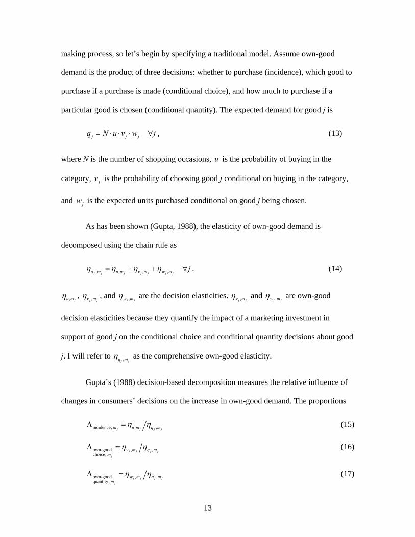
Decision-based decompositions require a model of the consumers’ decision-

13

making process, so let’s begin by specifying a traditional model. Assume own-good

demand is the product of three decisions: whether to purchase (incidence), which good to

purchase if a purchase is made (conditional choice), and how much to purchase if a

particular good is chosen (conditional quantity). The expected demand for good j is

j j jq N u v w j= ⋅ ⋅ ⋅ ∀ , (13)

where N is the number of shopping occasions, u is the probability of buying in the

category, jv is the probability of choosing good j conditional on buying in the category,

and jw is the expected units purchased conditional on good j being chosen.

As has been shown (Gupta, 1988), the elasticity of own-good demand is

decomposed using the chain rule as

, , , ,j j j j j j jq m u m v m w m jη η η η= + + ∀ . (14)

, ju mη , ,j jv mη , and ,j jw mη are the decision elasticities. ,j jv mη and ,j jw mη are own-good

decision elasticities because they quantify the impact of a marketing investment in

support of good j on the conditional choice and conditional quantity decisions about good

j. I will refer to ,j jq mη as the comprehensive own-good elasticity.

Gupta’s (1988) decision-based decomposition measures the relative influence of

changes in consumers’ decisions on the increase in own-good demand. The proportions

incidence, , ,j j j jm u m q mη ηΛ = (15)

own-good , ,choice,

j j j jj

v m q mm

η ηΛ = (16)

own-good , ,quantity,

j j j jj

w m q mm

η ηΛ = (17)

14

summarize the relationship and can be interpreted as follows: Of the growth in own-good

demand, incidence, jmΛ % is generated by consumers buying more frequently in the category,

own-goodchoice, jm

Λ % is generated by consumers choosing the target good more frequently when

they do buy in the category, and own-goodquantity, jm

Λ % is generated by consumers buying in greater

amounts when they do choose the target good.

The influence of changes in consumers’ decisions on the demand for competing

goods can be quantified in a similar manner. The elasticity of demand for a single

competing good is decomposed as

, , , ,k j j k j k jq m u m v m w m k jη η η η= + + ∀ ≠ . (18)

(Proof in appendix.) , ju mη represents the purchase incidence elasticity. The same term

appears in the own-good decomposition, as given in equation (14), because competing

goods benefit just like the target good does if consumers buy more frequently in the

category and their other decisions are held constant. ,k jv mη is the elasticity of conditional

cross-good choice, and ,k jw mη is the elasticity of conditional cross-good quantity.

Traditionally4, it has been assumed that the marketing actions of good j do not affect the

conditional cross-good quantity decisions, which implies , 0k jw m k jη = ∀ ≠ . In keeping

with this assumption, the elasticity of cross-good demand reduces to

, , ,k j j k jq m u m v m k jη η η= + ∀ ≠ . (19)

4 In making this assumption, Van Heerde et al. (2003, p. 489) note that it is… “used in all five major decomposition articles (Bell et al., 1999; Bucklin et al., 1999; Chiang, 1999; Chintagunta, 1993; Gupta, 1988).”

15

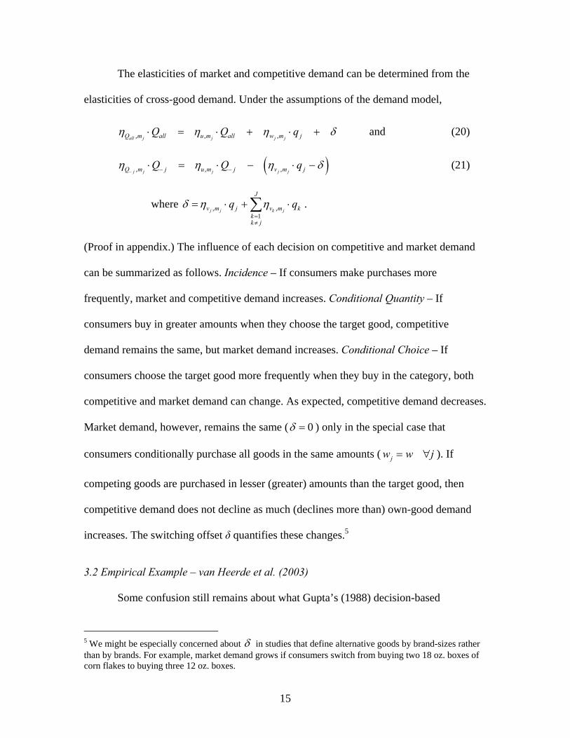
The elasticities of market and competitive demand can be determined from the

elasticities of cross-good demand. Under the assumptions of the demand model,

, , ,all j j j jQ m all u m all w m jQ Q qη η η δ⋅ = ⋅ + ⋅ + and (20)

( ), , ,j j j j jQ m j u m j v m jQ Q qη η η δ− − −⋅ = ⋅ − ⋅ − (21)

where , ,1

j j k j

J

v m j v m kkk j

q qδ η η=≠

= ⋅ + ⋅∑ .

(Proof in appendix.) The influence of each decision on competitive and market demand

can be summarized as follows. Incidence – If consumers make purchases more

frequently, market and competitive demand increases. Conditional Quantity – If

consumers buy in greater amounts when they choose the target good, competitive

demand remains the same, but market demand increases. Conditional Choice – If

consumers choose the target good more frequently when they buy in the category, both

competitive and market demand can change. As expected, competitive demand decreases.

Market demand, however, remains the same ( 0δ = ) only in the special case that

consumers conditionally purchase all goods in the same amounts ( jw w j= ∀ ). If

competing goods are purchased in lesser (greater) amounts than the target good, then

competitive demand does not decline as much (declines more than) own-good demand

increases. The switching offset δ quantifies these changes.5

3.2 Empirical Example – van Heerde et al. (2003)

Some confusion still remains about what Gupta’s (1988) decision-based

5 We might be especially concerned about δ in studies that define alternative goods by brand-sizes rather than by brands. For example, market demand grows if consumers switch from buying two 18 oz. boxes of corn flakes to buying three 12 oz. boxes.

16

decomposition means. To clarify its meaning and to ensure full understanding of its use

in section four, let’s reconsider his decomposition in the context of van Heerde et al.’s

(2003, p. 484) coffee example. Suppose there are 1000 shopping occasions in a given

week for coffee. The probability of purchasing coffee on any of these occasions is 0.20,

and the conditional probability of choosing Folgers given that coffee is purchased is 0.18.

The conditional quantity purchased is 1.0 unit, no matter which brand is chosen. The

elasticity of purchase incidence is , 0.034ju mη = , of conditional choice is , 0.210

j jv mη = ,

and of conditional quantity is , 0.004j jw mη = in response to feature-and-display

promotion. The comprehensive elasticity of own-good demand is , 0.248j jq mη = .

Van Heerde et al. (2003) incorrectly presume that Gupta’s (1988) decomposition

holds market demand constant in order to predict the change in competitive demand.

They write:

If we hold category demand constant at 200 units, then under this promotion the non-

promoted brands together sell 0.782 * 200 = 156.4 units. This represents a gross decline

of 7.6 units from the original sales of 164 units…

Category incidence is not constant, because the incidence probability is now 1.034 * 0.20

= 0.207. This leads to 0.207 *1000 = 207 purchase incidents. According to the model, of

the 7 additional purchase incidents, 78.2% should result in the purchase of non-promoted

brands, leading to an increase of 0.728 * 7 = 5.4 units. Thus, the net change in sales for

non-promoted brands equals -7.6 + 5.4 = -2.2 units (net total sales for the non-promoted

brands is 161.8 units).

Applying similar reasoning to the target good, however, leads to a contradiction.

The sales of Folgers would increase by 7.6 units if the demand for coffee remained the

same. But the demand for coffee would increase, and of the 7 additional purchase

incidents, 21.8% would result in purchases of 1.004 units of Folgers, leading to an

increase of 0.218 * 7 * 1.004 = 1.5 units. Thus, the change in sales of Folgers would be

17

7.6 + 1.5 = 9.1 units.6 This result is problematic, however, because the comprehensive

elasticity predicts that the demand for Folgers would grow by 0.248 * 36 = 8.9 units.

Van Heerde et al’s (2003) reasoning is incorrect for two reasons. Gupta’s (1988)

decomposition predicts how the changes in consumers’ decisions would affect only own-

good demand, not competitive demand. Furthermore, when calculating the influence of

any one decision on the growth in own-good demand, Gupta’s decomposition holds the

consumers’ other decisions constant, but does not hold the market demand constant. The

proper calculation is based on equation (14). The demand for Folgers would increase by

0.034 * 36 = 1.2 units due to consumers buying coffee more frequently, by 0.210 * 36 =

7.6 units due to consumers choosing Folgers more frequently when they do buy coffee,

and by 0.004 * 36 = 0.1 units due to consumers buying coffee in greater amounts when

they do buy Folgers. In total, the demand for Folgers would increase by 1.2 + 7.6 + 0.1 =

8.9 units due to the promotion, which reconciles with calculation based on the

comprehensive elasticity.

Competitive demand must be decomposed in order to determine how the changes

in consumers’ decisions would influence the demand for other coffees. Using equation

(21), the demand for other coffees would decrease by 0.210 * 36 = 7.6 units due to

consumers choosing to buy Folgers more frequently when they do buy coffee. The

switching offset would be zero in this example because the conditional purchase quantity

is assumed to be the same for all goods ( 1jw j= ∀ ). But the demand for other coffees

would increase by 0.034 * 164 = 5.6 units due to consumers buying coffee more

frequently. In total, the demand for other coffees would change by -7.6 + 5.6 = -2.0 units

6 Making matters somewhat more confusing, van Heerde et al. (2003) state the demand for Folgers increases by 9.2 units. This may be a simple arithmetic mistake.

18

due to the promotion, not -2.2 units.

Due to this error, a number of the studies that van Heerde et al. (p.483, Table 2)

quote as having misinterpreted Gupta’s findings actually interpret his findings correctly.

For example, they cite Chiang (1991, p. 309) who writes, “These results are similar to the

ones obtained by Gupta (1998, p. 352), where 84% of the increase is due to brand

switching, 14% by purchase time acceleration, and 2% by increases in quantity.”

Interpretations, like this one, that suggest Gupta’s findings attribute the growth in own-

good demand to changes in consumers’ decisions are correct.

Other studies quoted by van Heerde et al. (2003) do misinterpret Gupta’s findings.

For example, they cite Sethuraman and Srinivasan (2002, p.380) who write, “Gupta

(1988) and Bell, Chiang and Padmanabhan (1999) show that promotions have a relatively

small effect on category expansion compared with brand switching. Therefore, we isolate

and study the profitability due to brand switching only.” This conclusion cannot be drawn

from Gupta’s findings. Holding the consumers’ other decisions constant, greater purchase

frequency can lead to more growth in competitive demand than it would in own-good

demand. (In the example, the demand for other coffees would grow by 5.6 units due to

greater purchase frequency even though the demand for Folgers would grow only by 1.2

units.) Thus, the market expansion is not necessarily small simply because greater

purchase frequency would create a small amount of own-good demand. Combining the

decompositions, as will be done in section four, will make the difference between these

two interpretations even more distinct.

4. Decompositions that Measure Both Consumer and Competitive Impact

It is possible to measure the consumer and competitive impact of a promotion at

19

the same time. Unified decompositions quantify how a marketing action changes the

consumers’ decisions of whether, which, and how much to buy and how the change in

each of these decisions affects the own-good, competitive, and market demand. I will

show how the decision-based decomposition and unit- and share-based decompositions

relate to each other and will return to the coffee example to discuss what can be learned

from combining them.

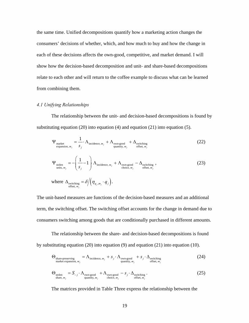
4.1 Unifying Relationships

The relationship between the unit- and decision-based decompositions is found by

substituting equation (20) into equation (4) and equation (21) into equation (5).

market incidence, own-good switchingexpansion, quantity, offset,

1j

j j j

mm m mjs

Ψ = ⋅Λ + Λ + ∆ (22)

stolen incidence, own-good switching units, choice, offset,

1 1j

j j j

mm m mjs

⎛ ⎞Ψ = − − ⋅Λ + Λ − ∆⎜ ⎟⎜ ⎟

⎝ ⎠, (23)

where ( )switching ,offset,

j jj

q m jm

qδ η∆ = ⋅ .

The unit-based measures are functions of the decision-based measures and an additional

term, the switching offset. The switching offset accounts for the change in demand due to

consumers switching among goods that are conditionally purchased in different amounts.

The relationship between the share- and decision-based decompositions is found

by substituting equation (20) into equation (9) and equation (21) into equation (10).

share-preserving incidence, own-good switchingmarket expansion, quantity, offset,

jj j j

m j jm m m

s sΘ = Λ + ⋅Λ + ⋅∆ (24)

stolen own-good own-good switchingshare, quantity, choice, offset, j j j j

j jm m m m

S s−Θ = ⋅Λ +Λ − ⋅∆ . (25)

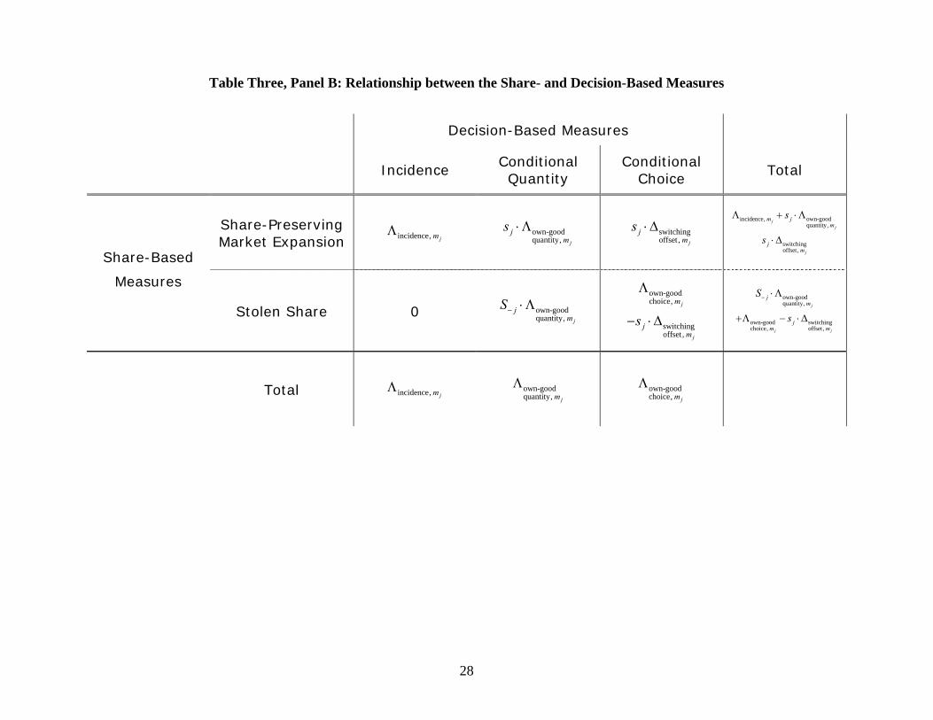
The matrices provided in Table Three express the relationship between the

20

consumer- and competitive-impact decompositions. Panel A depicts the relationship

between the decision- and unit-based decompositions and Panel B depicts the relationship

between the decision- and share-based decompositions. The cross-good elasticity

decomposition is critical to this analysis because it quantifies how changes in each of the

consumers’ decisions influence competitive and market demand.

< Insert Table Three >

The matrices clarify how each of the decompositions accounts for changes in

demand. First, it is interesting to note that the information contained in Gupta’s (1988)

decision-based decomposition is not sufficient to exactly determine the impact of a

marketing action on the demand for competing goods. The switching offset needs to be

determined in addition to the proportions given in equations (15) to (17) in order to

calculate the competitive impact. This is not troubling, however, because the intent of his

decomposition is to measure the relative influence of changes in each of the consumers’

decision on the growth in own-good demand. An analysis of the impact on cross-good

demand, which is required by the competitive-impact decompositions, is not necessary.

Second, strictly speaking, the measure of primary and secondary demand

proposed by Bell et al. (1999) can be given neither a unit- nor a share-based

interpretation. They define primary demand as the sum of the incidence and conditional

own-good quantity proportions, incidence, jmΛ and own-goodquantity, jm

Λ , and secondary demand as the

conditional own-good choice proportion, own-goodchoice, jm

Λ . While their measure of primary and

secondary demand is equivalent to neither of the competitive-impact measures, it does

closely approximate share-based measure when two conditions are met: (1) when the

proportion of own-good demand that is generated by the conditional own-good quantity

21

decision is small, own-goodquantity,

0jm

Λ ≈ , and (2) when the switching offset is small, 0δ ≈ . This

approximation may be useful in interpreting previously published results.

Third, it is easy to determine why the general relationship between the decision-

and unit-based decompositions is simpler in the special case that the conditional own-

good purchase quantity is the same for all goods. Van Heerde et al. (2003) show that if

jw w= j∀ , then

market stolenexpansion, units,

1j jm m

Ψ = −Ψ (26)

stolen incidence, choice onunits, own-good,

1j

j j

jm

m mj

vv

⎛ ⎞−Ψ = − ⋅Λ + Λ⎜ ⎟⎜ ⎟

⎝ ⎠. (27)

These relationships hold because the market share of each good is equivalent to its

conditional choice probability and the switching offset is zero in this special case. These

approximations are useful only when marketing actions have a weak influence on the

consumers’ conditional own-good quantity decisions, , 0j jw mη ≈ j∀ .The conditional

own-good quantities are sure to vary across goods, jw w≠ j∀ , if marketing actions

influence these decisions.

4.2 Coffee Example Revisited

Let’s revisit the coffee example to further illustrate the relationships between the

decompositions. The changes in own-good and competitive demand due to each of the

consumers’ decisions were determined in section three. The change in market demand,

which is also needed, can be constructively determined from equation (20). The demand

for coffee would increase by 0.034 * 200 = 6.8 units due to consumers buying coffee

more frequently and 0.004 * 36 = 0.1 units due to greater amounts of coffee being

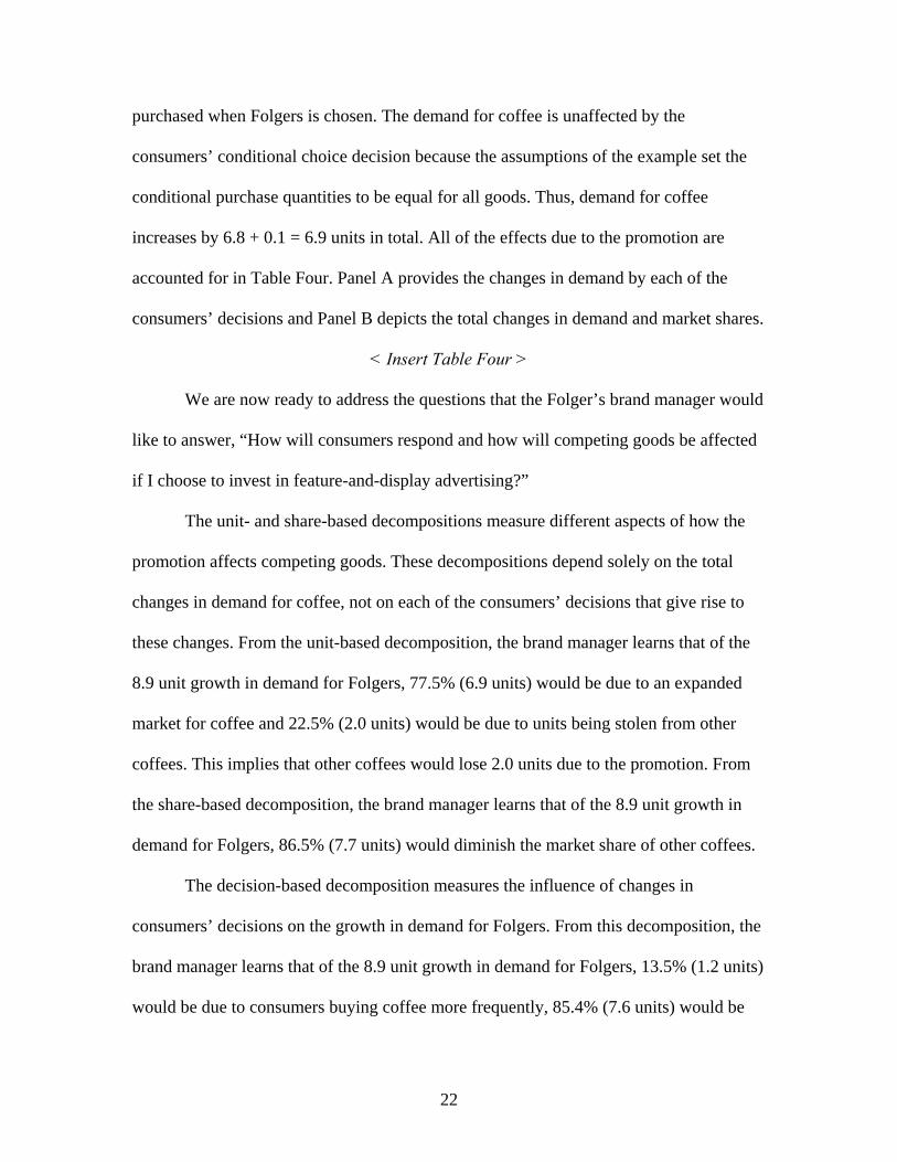
22

purchased when Folgers is chosen. The demand for coffee is unaffected by the

consumers’ conditional choice decision because the assumptions of the example set the

conditional purchase quantities to be equal for all goods. Thus, demand for coffee

increases by 6.8 + 0.1 = 6.9 units in total. All of the effects due to the promotion are

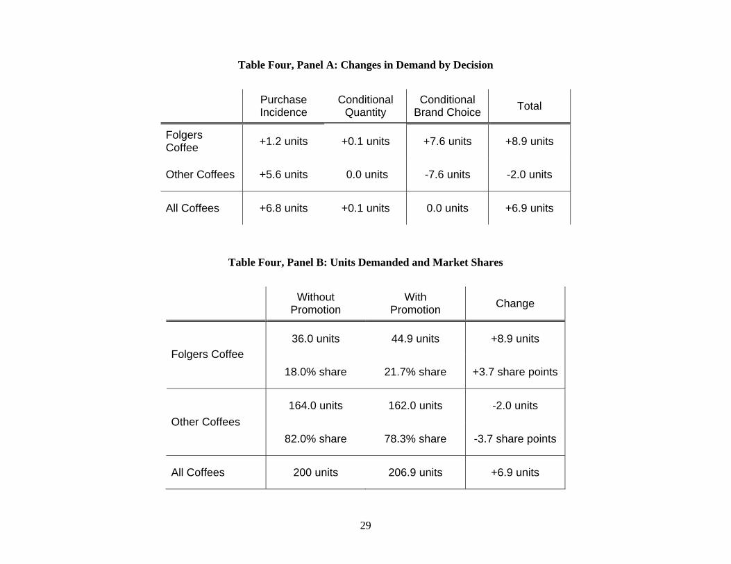
accounted for in Table Four. Panel A provides the changes in demand by each of the

consumers’ decisions and Panel B depicts the total changes in demand and market shares.

< Insert Table Four >

We are now ready to address the questions that the Folger’s brand manager would

like to answer, “How will consumers respond and how will competing goods be affected

if I choose to invest in feature-and-display advertising?”

The unit- and share-based decompositions measure different aspects of how the

promotion affects competing goods. These decompositions depend solely on the total

changes in demand for coffee, not on each of the consumers’ decisions that give rise to

these changes. From the unit-based decomposition, the brand manager learns that of the

8.9 unit growth in demand for Folgers, 77.5% (6.9 units) would be due to an expanded

market for coffee and 22.5% (2.0 units) would be due to units being stolen from other

coffees. This implies that other coffees would lose 2.0 units due to the promotion. From

the share-based decomposition, the brand manager learns that of the 8.9 unit growth in

demand for Folgers, 86.5% (7.7 units) would diminish the market share of other coffees.

The decision-based decomposition measures the influence of changes in

consumers’ decisions on the growth in demand for Folgers. From this decomposition, the

brand manager learns that of the 8.9 unit growth in demand for Folgers, 13.5% (1.2 units)

would be due to consumers buying coffee more frequently, 85.4% (7.6 units) would be

23

due to consumers choosing Folgers more frequently when they choose to buy coffee, and

1.1% (0.1 units) would be due to consumers purchasing coffee in greater amounts when

they choose to buy Folgers. This analysis focuses solely on the growth in demand for

Folgers, not on the changes in demand for other coffees.

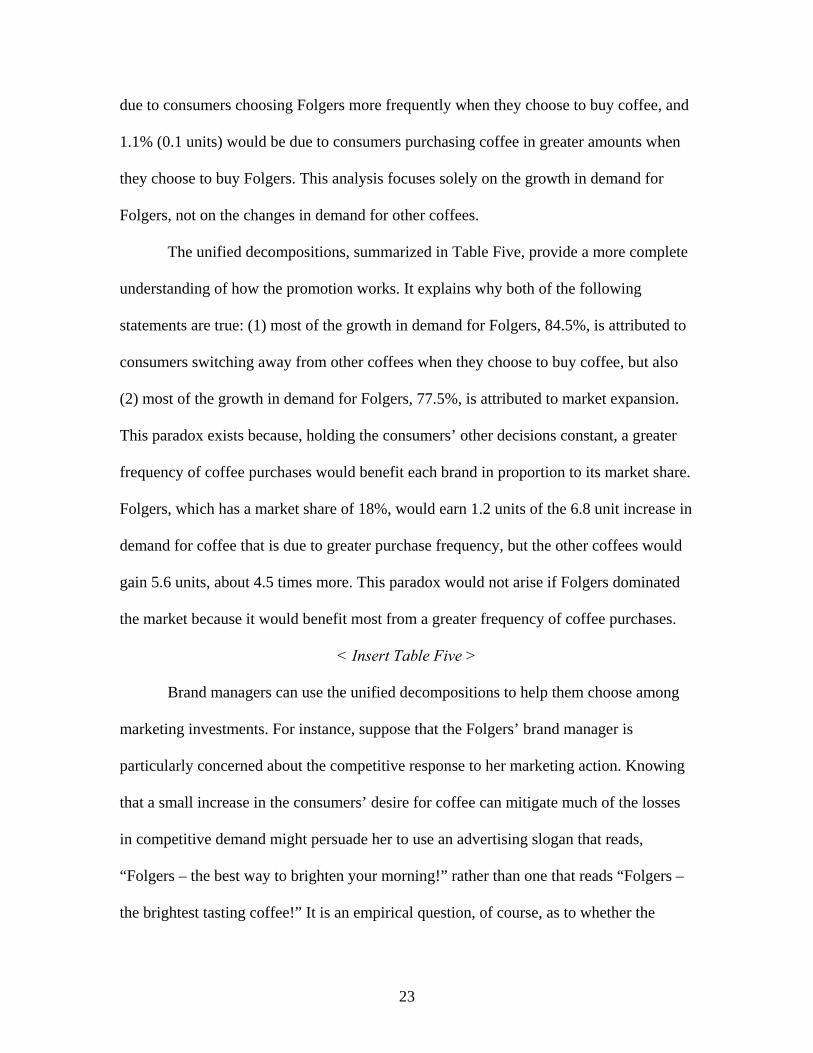
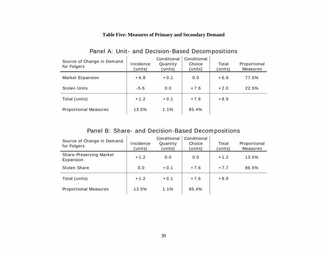
The unified decompositions, summarized in Table Five, provide a more complete

understanding of how the promotion works. It explains why both of the following

statements are true: (1) most of the growth in demand for Folgers, 84.5%, is attributed to

consumers switching away from other coffees when they choose to buy coffee, but also

(2) most of the growth in demand for Folgers, 77.5%, is attributed to market expansion.

This paradox exists because, holding the consumers’ other decisions constant, a greater

frequency of coffee purchases would benefit each brand in proportion to its market share.

Folgers, which has a market share of 18%, would earn 1.2 units of the 6.8 unit increase in

demand for coffee that is due to greater purchase frequency, but the other coffees would

gain 5.6 units, about 4.5 times more. This paradox would not arise if Folgers dominated

the market because it would benefit most from a greater frequency of coffee purchases.

< Insert Table Five >

Brand managers can use the unified decompositions to help them choose among

marketing investments. For instance, suppose that the Folgers’ brand manager is

particularly concerned about the competitive response to her marketing action. Knowing

that a small increase in the consumers’ desire for coffee can mitigate much of the losses

in competitive demand might persuade her to use an advertising slogan that reads,

“Folgers – the best way to brighten your morning!” rather than one that reads “Folgers –

the brightest tasting coffee!” It is an empirical question, of course, as to whether the

24

former slogan entices more consumers to drink coffee in the morning. But the unified

decompositions provide a means of testing how each of these marketing actions would

change consumers’ decisions, and, in turn, how the changes in each of these decisions

influence own-good and competitive demand.

5. Conclusion

Marketing investments are designed to change consumer behavior in ways that

help goods compete in the marketplace. Previous work has focused on how marketing

investments affect either consumer decision making or how they affect competing goods.

Decision-based decompositions attribute the growth in own-good demand to changes in

the consumers’ decision-making process. Unit- and share-based decompositions, on the

other hand, attribute the same growth to either rivalrous or non-rivalrous sources.

Combining the consumer and the competitive points of view in a single decomposition

provides a more complete understanding of the marketing investment’s impact, which

should lead to better managerial decisions. All of the methods that were discussed in this

article study a marketing investment’s contemporaneous effects. Future work might focus

on how the effects of an investment persist over time.

25

Table One: Units Demanded and Market Shares

Without

Incremental Advertising

With Incremental Advertising

Difference

500 units 530 units +30 units Firm A

33.3% share 34.6% share +1.3 share points

1000 units 1000 units No change Firm B

66.7% share 65.4% share -1.3 share points

Market Totals 1500 units 1530 units +30 units

26

Table Two: Comparison of Unit- and Share-Based Decompositions

Unit-Based Measures

Share-Based Measures

Drug Market Share

Primary Demand

Secondary Demand

Primary Demand

Secondary Demand

Tagamet 25% 0.929 0.071 0.232 0.768

Zantac 75% 0.634 0.366 0.476 0.524

Table Three, Panel A: Relationship between the Unit- and Decision-Based Measures

Decision-Based Measures

Incidence Conditional Quantity

Conditional Choice

Total

Market Expansion incidence,1

jmjs⋅Λ own-good

quantity, jmΛ switching

offset , jm∆ incidence, own-good

quantity,

switchingoffset,

1j

j

j

mmj

m

s⋅Λ + Λ

+∆

Unit-Based

Measures

Stolen Units incidence,1 1

jmjs

⎛ ⎞− − ⋅Λ⎜ ⎟⎜ ⎟⎝ ⎠

0 own-good switchingchoice, offset ,j jm m

Λ −∆ incidence,

own-good switchingchoice, offset,

1 1j

j j

mj

m m

s⎛ ⎞

− − ⋅Λ⎜ ⎟⎜ ⎟⎝ ⎠+Λ −∆

Total incidence, jmΛ own-goodquantity, jm

Λ own-goodchoice, jm

Λ

28

Table Three, Panel B: Relationship between the Share- and Decision-Based Measures

Decision-Based Measures

Incidence Conditional Quantity

Conditional Choice

Total

Share-Preserving Market Expansion incidence, jmΛ own-good

quantity, j

jm

s ⋅Λ switchingoffset , j

jm

s ⋅∆ incidence, own-good

quantity,

switchingoffset,

jj

j

m jm

jm

s

s

Λ + ⋅Λ

⋅∆

Share-Based

Measures

Stolen Share 0 own-goodquantity, j

jm

S− ⋅Λ own-goodchoice,

switchingoffset ,

j

j

m

jm

s

Λ

− ⋅∆

own-goodquantity,

own-good switchingchoice, offset,

j

j j

jm

jm m

S

s

− ⋅Λ

+Λ − ⋅∆

Total incidence, jmΛ own-goodquantity, jm

Λ own-goodchoice, jm

Λ

29

Table Four, Panel A: Changes in Demand by Decision

Purchase Incidence

Conditional Quantity

Conditional Brand Choice Total

Folgers Coffee +1.2 units +0.1 units +7.6 units +8.9 units

Other Coffees +5.6 units 0.0 units -7.6 units -2.0 units

All Coffees +6.8 units +0.1 units 0.0 units +6.9 units

Table Four, Panel B: Units Demanded and Market Shares

Without Promotion

With Promotion Change

36.0 units 44.9 units +8.9 units Folgers Coffee

18.0% share 21.7% share +3.7 share points

164.0 units 162.0 units -2.0 units Other Coffees

82.0% share 78.3% share -3.7 share points

All Coffees 200 units 206.9 units +6.9 units

30

Table Five: Measures of Primary and Secondary Demand

Panel A: Unit- and Decision-Based Decompositions

Source of Change in Demand for Folgers

Incidence (units)

Conditional Quantity (units)

Conditional Choice (units)

Total (units)

Proportional Measures

Market Expansion +6.8 +0.1 0.0 +6.9 77.5%

Stolen Units -5.6 0.0 +7.6 +2.0 22.5%

Total (units) +1.2 +0.1 +7.6 +8.9

Proportional Measures 13.5% 1.1% 85.4%

Panel B: Share- and Decision-Based Decompositions

Source of Change in Demand for Folgers

Incidence (units)

Conditional Quantity (units)

Conditional Choice (units)

Total (units)

Proportional Measures

Share-Preserving Market Expansion

+1.2 0.0 0.0 +1.2 13.5%

Stolen Share 0.0 +0.1 +7.6 +7.7 86.5%

Total (units) +1.2 +0.1 +7.6 +8.9

Proportional Measures 13.5% 1.1% 85.4%

Figure One

32

Figure Two

33

References

Bell, David R., Jeongwen Chiang, and V. Padmanabhan (1999), “The Decomposition of Promotional Response: An Empirical Generalization,” Marketing Science, 18, 504-526. Berndt, Ernst R., Linda Bui, David H. Reiley, and Glen L. Urban (1995), “Information, Marketing, and Pricing in the U.S. Anti-Ulcer Drug Market,” American Economic Review, 85, 2, 100-105. Berndt, Ernst R., Linda Bui, David H. Lucking-Reiley, and Glen L. Urban (1997), “The Roles of Marketing, Product Quality and Price Competition in the Growth and Composition of the U.S. Anti-Ulcer Drug Industry,” in The Economics of New Goods, Timothy F. Bresnahan and Robert J. Gordon, eds. Chicago, Illinois: University of Chicago Press, p. 277-328. Bucklin, Randolph E., Sunil Gupta, and S. Siddarth (1998), “Determining Segmentation in Sales Response Across Consumer Purchase Behaviors,” Journal of Marketing Research, 35, 189-197. Chiang, Jeongwen (1991), “A Simultaneous Approach to the Whether, What, and How Much to Buy Questions,” Marketing Science, 10, 297-315. Chintagunta, Pradeep K. (1993), “Investigating Purchase Incidence, Brand Choice, and Purchase Quantity Decisions of Households,” Marketing Science, 12, 184-208. Gupta, Sunil (1988), “Impact of Sales Promotions on When, What, and How Much to Buy,” Journal of Marketing Research, 25, 4, 342-55. Rosenthal, Meredith B., Ernst R. Berndt, Julie M. Donohue, Arnold M. Epstein, and Richard G. Frank (2003), “Demand Effects of Recent Changes in Prescription Drug Promotion,” in Frontiers in Health Policy Research, Volume 6, David M. Cutler and Alan M. Garber, eds. Cambridge, Massachusetts: The MIT Press, p. 1-26. Sethuraman, Raj and V. Srinivasan (2002), “The Asymmetric Share Effect: An Empirical Generalization of Cross-Price Effects,” Journal of Marketing Research, 39, 3, 379-86. Van Heerde, Harald J., Sachin Gupta, and Dick R. Wittink (2003), “Is 75% of the Sales Promotion Bump Due to Brand Switching? No, Only 33% Is,” Journal of Marketing Research, 40, 4, 481-491. Van Heerde, Harald J., Peter S. H. Leeflang, and Dick R. Wittink (2004), “Decomposing the Sales Promotion Bump with Store Data,” Marketing Science, 23, 3, 317-334.

34

Technical Appendix

Proposition: The change in own-good demand can be decomposed as

j jall allj j

j j j j

q QQ Qs Sm m m m

−−

⎡ ⎤∂ ∂∂ ∂= ⋅ − + ⋅⎢ ⎥

∂ ∂ ∂ ∂⎢ ⎥⎣ ⎦.

Proof:

( )

( )

2

1

1

jjall all

j j

j allall

j

j jallall

j all j all

j allj

j j

SsQ Q

m m

Q QQ

m

Q QQQm Q m Q

Q QSm m

−

−

− −

−−

⎡ ⎤∂ −∂⎢ ⎥⋅ = ⋅

∂ ∂⎢ ⎥⎣ ⎦⎡ ⎤∂ −⎢ ⎥= ⋅

∂⎢ ⎥⎣ ⎦⎡ ⎤∂ ∂

= − ⋅ ⋅ − ⋅⎢ ⎥∂ ∂⎢ ⎥⎣ ⎦

⎡ ⎤∂ ∂= − − ⋅⎢ ⎥

∂ ∂⎢ ⎥⎣ ⎦

Thus,

j jallj all

j j j

jall allj j

j j j

q sQs Qm m m

QQ Qs Sm m m

−−

∂ ∂∂= ⋅ + ⋅

∂ ∂ ∂

⎡ ⎤∂∂ ∂= ⋅ − + ⋅⎢ ⎥

∂ ∂ ∂⎢ ⎥⎣ ⎦

Q.E.D.

35

Proposition: Assuming the demand model of equation (13), the cross-good elasticity of

demand is , , , ,k j j k j k jq m u m v m w mη η η η= + + .

Proof:

The demand for good k is

k k kq N u v w for k j= ⋅ ⋅ ⋅ ≠ .

Applying the chain rule yields

k k kk k k k

j j j j

q v wuN v w N u w N u vm m m m∂ ∂ ∂∂

= ⋅ ⋅ ⋅ + ⋅ ⋅ ⋅ + ⋅ ⋅ ⋅∂ ∂ ∂ ∂

.

Thus, the cross-good elasticity is

,

, , ,

k j

j k j k j

jkq m

j k

jk kk k k k

j j j k

j j jk k

j j k j k

u m v m w m

mqm q

mv wuN v w N u w N u vm m m q

m m mv wum u m v m w

η

η η η

∂= ⋅∂

⎛ ⎞∂ ∂∂= ⋅ ⋅ ⋅ + ⋅ ⋅ ⋅ + ⋅ ⋅ ⋅ ⋅⎜ ⎟⎜ ⎟∂ ∂ ∂⎝ ⎠

∂ ∂∂= ⋅ + ⋅ + ⋅∂ ∂ ∂

= + +

Q.E.D.

Proposition: Assuming the demand model of equation (13) and that , 0k jw m k jη = ∀ ≠ ,

, , ,all j j j jQ m all u m all w m jQ Q qη η η δ⋅ = ⋅ + ⋅ + .

Proof:

, ,1

, , ,1

all j k j

j k j k j

J

Q m all q m kkJ

u m v m w m kk

Q q

q

η η

η η η

=

=

⋅ = ⋅

⎡ ⎤= + + ⋅⎣ ⎦

∑

∑

36

, , ,1

, ,

j k j k j

j k j

J

u m all w m j v m kk

u m all w m j

Q q q

Q q

η η η

η η δ=

= ⋅ + ⋅ + ⋅

= ⋅ + ⋅ +

∑

where , ,1

j j k j

J

v m j v m kkk j

q qδ η η=≠

= ⋅ + ⋅∑

Q.E.D.

Proposition: Assuming the demand model of equation (13) and that , 0k jw m k jη = ∀ ≠ ,

( ), , ,j j j j jQ m j u m j v m jQ Q qη η η δ− − −⋅ = ⋅ − ⋅ − .

Proof:

, ,1

, , ,1

j j k j

j k j k j

J

Q m j q m kkk j

J

u m v m w m kkk j

Q q

q

η η

η η η

− −=≠

=≠

⋅ = ⋅

⎡ ⎤= + + ⋅⎣ ⎦

∑

∑

Assuming that , 0k jw m k jη = ∀ ≠ ,

, , ,1

, ,

j j j k j

j j j

J

Q m j u m j v m kkk j

u m j v m j

Q Q q

Q q

η η η

η η δ

− − −=≠

−

⋅ = ⋅ + ⋅

= ⋅ − ⋅ +

∑

where , ,1

j j k j

J

v m j v m kkk j

q qδ η η=≠

= ⋅ + ⋅∑

Q.E.D.