Measuring Consensus in Binary Forecasts: NFL Game Predictions

ChiUng Song

Science and Technology Policy Institute 26F., Specialty Construction Center 395-70

Shindaebang-dong, Tongjak-ku Seoul 156-714, Korea Tel: 822-3284-1773 cusong@stepi.re.kr

Bryan L. Boulier** Department of Economics

The George Washington University Washington, DC 20052

Tel: 202-994-8088 Fax: 202-994-6147 mortile@gwu.edu

Herman O. Stekler

Department of Economics The George Washington University

Washington, DC 20052 Tel: 202-994-6150 Fax: 202-994-6147 hstekler@gwu.edu

RPF Working Paper No. 2008-006 http://www.gwu.edu/~forcpgm/2008-006.pdf

July 8, 2008

RESEARCH PROGRAM ON FORECASTING Center of Economic Research

Department of Economics The George Washington University

Washington, DC 20052 http://www.gwu.edu/~forcpgm

Research Program on Forecasting (RPF) Working Papers represent preliminary work circulated for comment and discussion. Please contact the author(s) before citing this paper in any publications. The views expressed in RPF Working Papers are solely those of the author(s) and do not necessarily represent the views of RPF or George Washington University.

Measuring Consensus in Binary Forecasts: NFL Game Predictions

Keywords: binary forecasts, NFL, agreement, consensus, kappa coefficient ChiUng Song Science and Technology Policy Institute 26F., Specialty Construction Center 395-70 Shindaebang-dong, Tongjak-ku Seoul 156-714, Korea Tel: 822-3284-1773 cusong@stepi.re.kr Bryan L. Boulier** Department of Economics The George Washington University Washington, DC 20052 Tel: 202-994-8088 Fax: 202-994-6147 mortile@gwu.edu Herman O. Stekler Department of Economics The George Washington University Washington, DC 20052 Tel: 202-994-6150 Fax: 202-994-6147 hstekler@gwu.edu

July 8, 2008

**The corresponding author is Bryan L. Boulier.

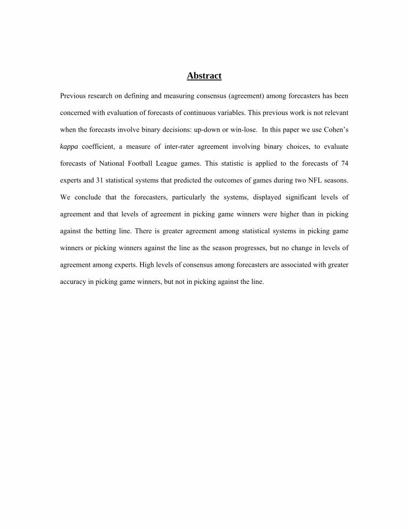
Abstract

Previous research on defining and measuring consensus (agreement) among forecasters has been

concerned with evaluation of forecasts of continuous variables. This previous work is not relevant

when the forecasts involve binary decisions: up-down or win-lose. In this paper we use Cohen’s

kappa coefficient, a measure of inter-rater agreement involving binary choices, to evaluate

forecasts of National Football League games. This statistic is applied to the forecasts of 74

experts and 31 statistical systems that predicted the outcomes of games during two NFL seasons.

We conclude that the forecasters, particularly the systems, displayed significant levels of

agreement and that levels of agreement in picking game winners were higher than in picking

against the betting line. There is greater agreement among statistical systems in picking game

winners or picking winners against the line as the season progresses, but no change in levels of

agreement among experts. High levels of consensus among forecasters are associated with greater

accuracy in picking game winners, but not in picking against the line.

1

Measuring Consensus in Binary Forecasts:

NFL Game Predictions

1. Introduction

Previous research on defining and measuring agreement or consensus among

forecasters has been concerned with evaluations of quantitative forecasts, i.e. GDP will

increase 4%, inflation will go up 2%, etc.. Procedures for determining whether

consensus among quantitative forecasts have evolved over time. Customarily the mean

or median of a set of forecasts had been used as the measure of “consensus”, but

Zarnowitz and Lambros (1987) noted that there was no precise definition of what

constituted a “consensus”. Lahiri and Teigland (1987) indicated that the variance across

forecasters was the appropriate measure of agreement or disagreement, while Gregory

and Yetman (2001) argued that a consensus implied that there was a majority view or

general agreement. Schnader and Stekler (1991) and Kolb and Stekler (1996) went

further and suggested that the methodology for determining whether a “consensus”

actually existed should be based on the distribution of the forecasts.

A number of questions about forecaster behavior have been analyzed using the

dispersion and distributions of these quantitative forecasts. For example, they have been

used to determine whether these data can provide information about the extent of

forecaster uncertainty (Zarnowitz and Lambros, 1987; Lahiri and Teigland, 1987; Lahiri

et al., 1988; Rich et al., 1992; Clements, 2008). Changes in the dispersion of the

2

forecasts have also been used to examine the time pattern of convergence of the forecasts

(Gregory and Yetman, 2004; Lahiri and Sheng, 2008).

To this point, there have been no analyses of the extent of agreement among

individuals who do not make quantitative predictions but rather issue binary forecasts:

up-down or win-lose. Moreover, the previous methodology applied to quantitative

forecasts is not relevant for binary forecasts. Fortunately, there is a statistical measure of

agreement, the kappa coefficient (Cohen, 1960; Landis and Koch, 1977), which can be

used to evaluate these types of binary forecasts. This coefficient is used extensively in

evaluating diagnostic procedures in medicine and psychology.

In this paper we use that coefficient to evaluate the levels of agreement among the

forecasts of 74 experts and 31 statistical systems for outcomes of National Football

League regular season games played during the 2000 and 2001 seasons. This data set is

the same used earlier to analyze the predictive accuracy of these experts and systems

(Song, et al., 2007). The experts and systems made two types of binary forecasts. They

either predicted whether a team would win a specific game or whether a particular team

would (not) beat the Las Vegas betting spread. Song, et al. (2007)concluded that the

difference in the accuracy of the experts and statistical systems in predicting game

winners was not statistically significant. Moreover, the betting market outperformed both

in predicting game winners and neither the experts not systems could profitably beat the

betting line.

In this paper, we are not concerned with the relative predictive accuracy of

experts and statistical systems and thus will not examine their forecasting records. Rather,

we are interested in knowing whether, in making these two types of binary forecasts, the

3

experts and systems generally agreed with one another. We will demonstrate that it is

possible to determine the degree of agreement among forecasters who make binary

forecasts and to test the hypothesis that there is a positive relationship between the extent

of agreement and the accuracy of forecasts.

The paper examines a number of issues relating to these forecasts: (1) whether

there is agreement within groups of forecasters (e.g., do experts agree with each other?),

(2) whether agreement changes as more information becomes available during the course

of a season, and (3) whether there is agreement between groups of forecasters (e.g., do

experts’ forecasts agree with those of systems?). We hypothesize that there is likely to be

considerable agreement among forecasters in forecasting the outcomes of NFL games,

because experts who make judgmental forecasts and statistical model builders share a

substantial amount of publicly available data. In addition, experts have access to many of

the predictions made by statistical systems prior to making their own forecasts. Thus, it

is possible that both experts and statistical systems make similar predictions, and their

forecasts are associated with each other. We also expect that agreement among

forecasters is likely to increase during the course of a season, since information on the

relative strength of teams emerges as the season progresses. Finally, we test the

hypothesis that accuracy is related to the extent of agreement.

Section 2 presents the data that will be analyzed in this study. Section 3 describes

methods for measuring the extent of agreement among forecasts. Section 4 examines the

degree of agreement among experts and statistical systems in (1) picking the home team

or the visiting team to win the game or (2) to beat the betting line. We first compare the

level of agreement among the predictions for an entire season and then examine whether

4

levels of agreement change over the course of a season. Having found that there is

substantial agreement among experts and among statistical systems in predicting the

outcomes of games, we then test whether agreement and accuracy are related.

2. Data

Our data consist of the forecasts of the outcomes of the 496 regular season NFL

games for the 2000 and 2001 seasons. These forecasts include those made by experts

using judgmental techniques, forecasts generated from statistical models, and a market

forecast – the betting line. The forecasts of 74 experts were collected from 14 daily

newspapers, 3 weekly magazines, and the web-sites of two national television networks.

The newspapers include USA Today, a national newspaper, and 13 local newspapers

selected from cities that have professional football teams. The three weekly national

magazines are Pro Football Weekly, Sports Illustrated, and The Sporting News. Two

television networks, CBS and ESPN, have web-sites that contain the forecasts of their

staffs.

Some experts predict game winners directly, while others make predictions

against the Las Vegas betting line. Some experts who pick game winners also predict the

margin of victory (i.e., a point spread). For those who predict a margin of victory, one

can identify their implicit picks against the line by comparing their predicted margin of

victory with the betting spread given by the Las Vegas betting line. The Las Vegas

betting line data were obtained from The Washington Post on the day that the game was

played. Appendix Table A summarizes information on the individual experts represented

in our analysis.

5

Todd Beck (www.tbeck.freeshell.org) collected the point spread predictions made

by 29 statistical models for the 2000 and 2001 NFL seasons. We used these data as well

as the predictions of the Packard and Greenfield systems, which were not included in

Beck’s sample. The point spread predictions allow us to identify both the predicted

winner of a game and the predicted winner against the betting line. The data used to

generate the point spread predictions vary across models, as do the statistical models used

to generate the forecasts. Among the data used to generate the point spread predictions

are the won/loss records of teams, offensive statistics (such as points scored or yards

gained), defensive statistics (such as points or yards allowed per game), variables

reflecting the strength of schedule, and home field advantage. In many of these models,

point spread predictions are based on power rankings of the teams. Appendix Table B

presents names of the statistical models whose forecasts were used in our analysis.

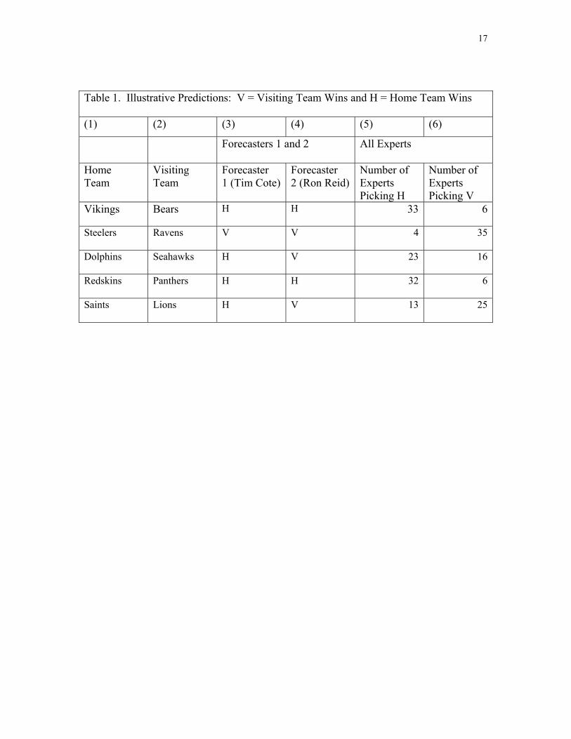
Table 1 gives an example of the kinds of data we are using. Columns (1) and (2)

identify the visiting and home teams for some of the games in the first week of the 2000

season. Columns (3) and (4) give the forecasts of two of the 74 experts in our sample.

Forecaster 1 is Tim Cote of the The Miami Herald and Forecaster 2 is Ron Reid of the

The Philadelphia Inquirer. Columns (5) and (6) summarize the forecasts made by all of

the experts who made predictions for these games. Similar data are available for the 31

systems.

<Table 1 about here>

3. Methods of analysis

To measure the extent of agreement among forecasters, we use the kappa

coefficient. The computation and interpretation of the kappa coefficient can be illustrated

6

using contingency table analysis. Before we present the procedure for calculating kappa

for our full sample of 74 experts and 31 systems, we illustrate our method using data for

two of the experts - Tim Cote (Forecaster 1) and Ron Reid (Forecaster 2).

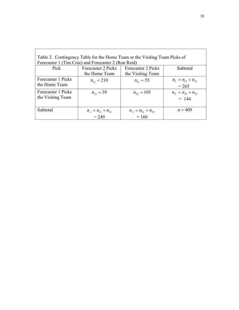
Table 2 is a contingency table that shows the distribution of forecasts of the two

individuals. There were 409 games in which both forecasters made predictions about

whether the home of visiting team would win the game. The elements along the diagonal

indicate the number of times both forecasters made the same predictions: the home

(visiting) team will win. That is, there were 210 games in which both picked the home

team to win and 105 games in which they both picked the away team to win for a total of

315 games for which they predicted the same outcome.

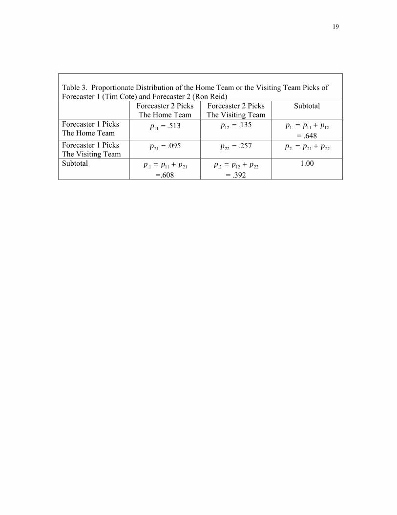
If we divide each entry in Table 2 by the total number of games ( n ), we obtain

the proportionate distribution of picks shown in Table 3, where p denotes the

proportionate distribution in row і and column j. From Table 3, we can determine

whether the picks of the two forecasters are independent or not, but we will need to

undertake further calculations, which are explained below, to see if there is agreement.

ij

<Table 3 about here>

The picks would be considered to be independent if the probability that forecaster 1 picks

the home team to win does not depend on whether forecaster 2 picks the home (or the

visiting) team to win. That is, knowledge of the picks of forecaster 2 provides no

information about predicting forecaster 1’s choices. If the picks are independent, then the

expected proportion, in cell ijep ( )ji, would be ji

eij ppp .. ×=

The hypothesis that the picks are independent can be tested using the chi-square

statistic (Fleiss, et al., 2003; pp. 53):

7

( )∑∑= =

−−=

2

1

2

1 ..

2

..22/1(

i j ji

jiij

pp

npppnχ , (1)

with one degree of freedom. For the data given in Table 2, the 106.59, which is

significantly different from zero at the 0.01 level, indicating that the forecasts are not

independent.

=2χ

Note that the magnitude of measures whether or not there is independence

between the forecasters but

2χ

not the level of agreement. There are two reasons why the

magnitude of does not measure agreement. First, the choices of the two forecasters

may depend upon each other, but reflect disagreement rather than agreement. Consider

two cases. In Table 3,

2χ

78.02211 =+ pp , so that individuals made identical forecasts 78%

of the time. But, suppose the data given in Table 3 were altered by switching the

diagonal and off-diagonal elements. In particular, assume that 135.11 =p ,

095.22 =p

2χ

, , and . With this distribution of forecasts the value of

would remain 106.59, but the individuals would have made identical forecasts only

22% of the time.

513.12 =p 257.21 =p

Second, the size of reflects not only the pattern of disagreement or

disagreement among forecasters but also the number of forecasts. That is, for a given

proportional distribution of forecasts (i.e., the ), the magnitude of is (essentially)

linearly related to the number of forecasts (n). (See equation (1).) Consequently, if one

were to use the as a measure of agreement, one would infer higher levels of

agreement between two forecasters if they make a larger number of forecasts even though

2χ

ijp 2χ

2χ

8

the fraction of forecasts on which they agreed did not change. For example, suppose that

that Forecaster 1 and Forecaster 2 had predicted 818 games rather than 409 and that the

proportionate distribution of forecasts were identical to that shown in Table 3. With 818

forecasts, the size of would double to 213.38, even though the proportion of games

for which they made identical forecasts would remain unchanged at 0.78

2χ

As noted above, to examine the extent of agreement among forecasters, one must

compute the proportion of forecasts that are identical between the forecasters.1 The

proportion of forecasts that are identical is obtained by summing the entries along the

diagonal cells in the contingency tables. That is, the proportion of cases on which the two

individuals made the same forecasts is given by 22110 ppp += . However, there is a

disadvantage of using the simple proportion of picks that are the same as a measure of

agreement. One could obtain a high percentage of picks in common merely by chance

(Fleiss, et al., 2003, pp.602-608). To adjust for the role of chance, one should compare

the actual level of agreement with that based on chance alone.

The expected proportion of agreement (given independence in the picks) is given

by . The difference,( ) 2.1..1 ppppe +×= ( .2p × ) epp −0 , measures the level of agreement

in excess of that which would be expected by chance. Cohen (1960) suggested using the

kappa statistic (κ) as a measure of agreement that adjusts for chance selections2:

e

e

ppp

−−

=1

0κ .

1 As an alternative one could measure the extent of disagreement between the forecasters by summing the off diagonal elements ( ). Swanson and White (1997, p. 544) describe this measure as the “confusion rate”.

21pp12 +

2 The Associate Editor pointed out that the kappa coefficient is identical to the Heidke skill score. The Heidke skill score has been used in evaluating directional forecasts in the weather literature. See C.A. Doswell, et al. (1990) and Lahiri and Wang (2006).

9

For the data shown in Table 2, κ = .509, which is statistically significantly different from

zero at the 0.01 level.

While we have illustrated kappa for the case of two forecasters, it can be extended

to the case of multiple forecasters. (See Fleiss, et al., 2003, pp. 610-617.) Here we use

the kind of data shown in columns (5) and (6) in Table 1 - the number of forecasters who

picked the visiting team to win and the number who picked the home team to win for

each game. Assume there are n games and that the number of forecasters who predicted

the ith game is mi. Note that it is not assumed that the set of forecasters are identical for

each game. Let xi equal the number of forecasters picking the visiting team to win in the

ith game and mi - xi the number picking the home team. Let p equal the proportion of all

forecasts (i.e., all forecasts for all games combined) in which the visiting team is chosen

to win the game and let pq −= 1 be the proportion of all forecasts in which the home

team is picked to win. Finally, let m equal the average number of forecasts per game (i.e.,

the total number of forecasts for all games combined divided by the number of games).

Then, kappa is estimated by the following formula (Fleiss, et al, 2003, p. 610):

qpmnm

xmxn

i i

iii

)1(

)(1

−

−

=∑=κ .

The kappa statistic is sometimes called a measure of inter-rater agreement.

If , then κ = 0 and there is only chance agreement. If κ > 0, then there is

agreement over and above that due to chance, and there is less agreement than expected

by chance if κ < 0. If κ = 1, there is perfect agreement. The magnitude of the standard

epp =0

10

error can also be measured (Fleiss, et al., 2003, pp. 605 and 613), so that one can use this

standard deviation and the value of κ to determine whether κ is statistically significantly

different from zero. However, in comparing values of kappa across samples, we use

bootstrapping to determine whether there are statistically significant differences between

the coefficients (cf., McKenzie, et al, 1996).

What does the magnitude of κ signify? Landis and Koch (1977) suggested

guidelines for interpreting the strength of agreement based on the value of kappa. Their

guidelines are shown in Table 4.

<Table 4 about here>

4. Levels of agreement among experts and statistical systems

In this section, we compare the levels of agreement among experts and statistical

systems in picking the home team or the visiting team (1) to win the game or (2) to beat

the betting line. We first calculate kappa coefficients (κ) for inter-rater agreement for all

games of the 2000-2001 seasons. We then examine whether levels of agreement change

over the course of the season. It might be anticipated, for example, that levels of

agreement would increase as a season progresses, since the accumulation of information

during the course of a season would resolve uncertainties regarding the relative abilities

of teams.

<Table 5 about here>

Table 5 presents these results. The major findings for the two complete seasons

are:

11

(a) All the kappa coefficients are statistically significantly different from zero at

the 0.01 level. According to the Landis-Koch criteria, statistical systems display

moderate agreement, while experts exhibit fair agreement.

(b) There is substantially higher agreement among both types of forecasters in

picking game winners than in picking against the line.

(c) The levels of agreement among statistical systems are considerably higher

than among experts for both types of forecasts. Using a bootstrap procedure with 500

observations to calculate the standard errors of the difference, we find that these

differences are statistically significant at the 0.01 level.

A comparison of forecasts for first and second half games of the two seasons

indicates:

(d) Kappa coefficients calculated for each of the two halves replicate the full

season results reported above.

(e) Among statistical systems, levels of agreement in picking game winners and

picking against the line are higher in second half games than in first half games and these

differences across halves are statistically significantly different from zero at the 0.05

level. In contrast, the second half levels of agreement among experts are not statistically

significantly different from their first half levels. Thus, it would appear that statistical

systems process information in a way that resolves differences among their forecasts as

data accumulates, but that experts do not.3

5. Agreement among consensus forecasts by statistical systems, experts, and the

betting line

3 Of interest is that statistical system forecasts improve over the course of season, while those of experts do not. See Song, et al. (2007).

12

In this section, we measure the extent of agreement among statistical systems,

experts, and the betting line in picking game winners. In the preceding section, we found

that there was considerable agreement among statistical systems and also among experts

in picking game winners. Consequently, we can identify consensus picks for each of the

two sets of forecasters. We do this by selecting the team chosen to win the game by a

majority of the forecasters of each group. If there is no majority (e.g. if the number of

experts favoring the home team equals the number favoring the away team or if the

betting line is zero), we exclude that game from the analysis presented here.

Table 6 reports the values of kappa (1) for pairwise comparisons of the betting

line and consensus picks of statistical systems and experts and (2) of all three methods of

forecasting. These measures are calculated for the combined 2000-2001 NFL seasons

and for the first and second halves of the combined seasons.

<Table 6 about here>

In all cases, the magnitudes of κ are large, indicating substantial agreement, and

statistically significantly different from zero at the 0.01 level. For all games, the extent of

agreement between experts and the betting line is statistically significantly higher at the

0.05 level (two-tail test) than that of statistical experts and the betting line or than that of

statistical systems and experts.

6. The relationship between agreement and accuracy.

To this point we have focused on the degree of consensus among the various

forecasters and have not considered whether there is a relationship between the extent of

the agreement and the accuracy of the predictions. We examine four such relationships

in this section: experts’ and systems’ predictions of (1) game winners and (2) winners

13

against the betting spread. The extent of agreement for a game is measured by examining

the proportion of experts (or systems) agreeing on a winner.4 If 50% of forecasters

favors one team to win a game and 50% favors its opponent to win, then the game is

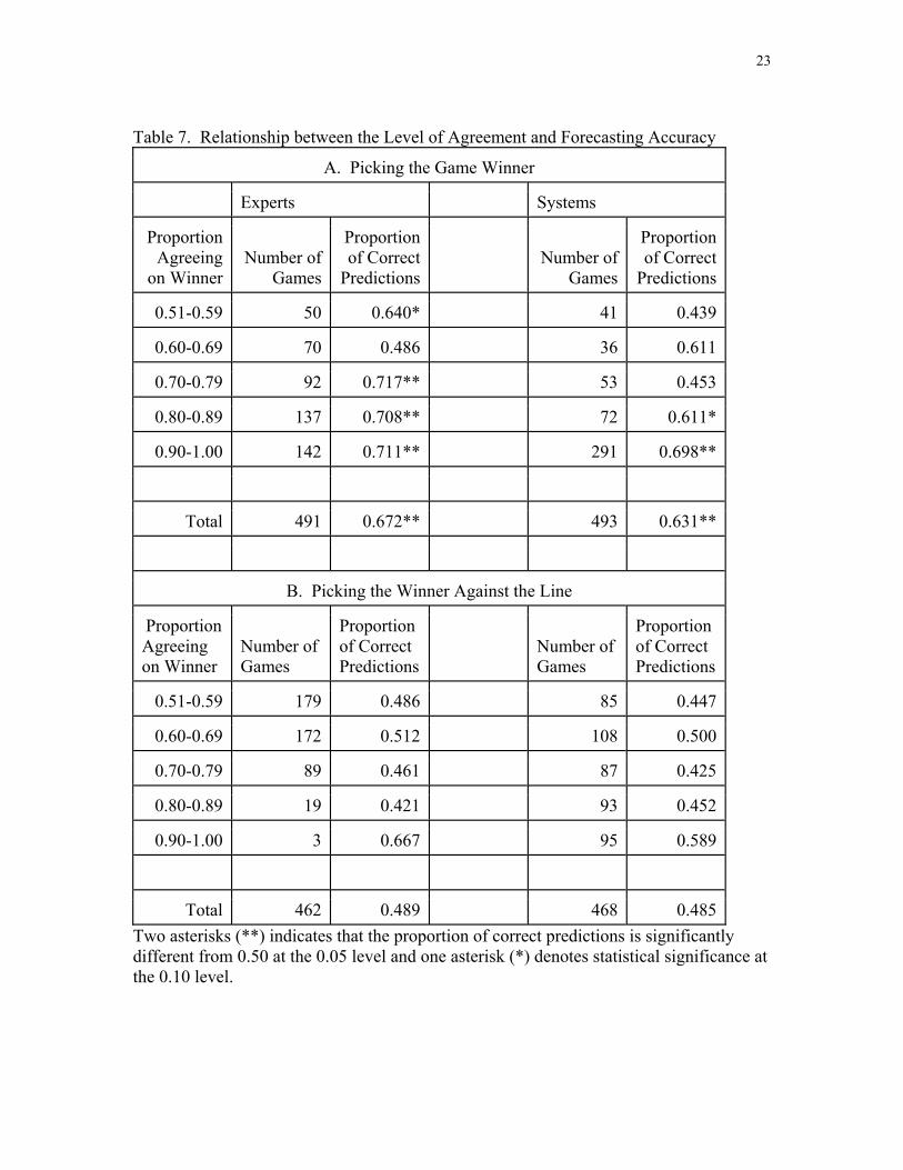
dropped from the sample. The results are presented in Table 7.

<Table 7 about here.>

There is not a monotonic relationship between agreement and accuracy in picking

game winners, although very high levels of agreement are associated with greater

accuracy. Experts have a success rate around 70% when 70% or more of experts are in

agreement (about three-fourths of the games). These success rates are statistically

significantly different from 0.50 at the 0.01 level. When 90% or more of systems agree

on the outcome (about 6 out of 10 games), they also have a 70% success rate, also

statistically significantly different from 0.50 at the 0.01 level.

The results are quite different for picking winners against the line. In order for

bets against the line to be profitable, a 52.4% success ratio is required. Both experts and

systems, however, had success ratios that were usually less than 50%. Moreover, the

success rates of experts in picking against the line do not vary with the extent of

agreement. Even when 70% or more of the experts are in agreement, they only pick

correctly 46% of the winners against the line.5 As for systems, only when 90% or more

of the systems agreed whether a particular team would (not) cover the spread was the

result significant. The accuracy rate of nearly 60% was statistically different (at the 0.05

4 In Table 7, each individual game is an observation. The kappa statistic is useful only when comparing agreement among two or more forecasters for multiple games. 5 A referee suggested that since they were wrong 54% of the time and an accuracy rate of 52.4% is sufficient to be profitable, one might have made money by betting against the experts. Whether this result would hold in another set of games is problematical. A failure rate of 0.54 or larger would occur 22% of the time if the experts’ true inability for picking winners were equal to flipping a coin (one tail test).

14

level) from flipping a coin, but not statistically significantly different, even at the 0.10

level, from the 52.4% rate necessary to bet profitably against the line.

7. Conclusion

In this study, we have compared levels of agreement among experts and statistical

systems in predicting game winners or picking against the line for the 2000 and 2001

NFL seasons using the kappa coefficient as a measure of agreement. We found that

there are highly statistically significant levels of agreement among forecasters in their

predictions, with a higher level of agreement among systems than among experts. In

addition, there is greater agreement among forecasters in picking game winners than in

picking against the betting line.

Finally, high levels of agreement among experts or forecasters are associated with

greater accuracy in forecasting game winners but not against picking winners against the

line. The previous literature that was concerned with the consensus of quantitative

forecasts has not focused on the accuracy of the predictions when there was (not) a

consensus. It would be desirable to do this.

15

References

Clements, M.P. (2008). Consensus and uncertainty: Using forecast probabilities of output declines. International Journal of Forecasting, 24, 76-86. Cohen, J. (1960). A coefficient of agreement for nominal scales, Educational and Psychological Measurement, 20, 37-46. Doswell, C.A., Davies-Jones, R. & Keller, D.L. (1990). On summary measures for skill in rare event forecasting based on contingency tables, Weather and Forecasting, 5, 576-585. Fleiss, J.L., Levin, B. and Paik, M.C. (2003), Statistical methods for rates and proportions, 3rd edition. New York: Wiley Series in Probability and Statistics. Gregory, A. W., Smith, G. W. & Yetman J. (2001). Testing for forecast consensus, Journal of Business and Economic Statistics, 19, 34-43. Gregory, A. W. & Yetman J. (2004). The evolution of consensus in macroeconomic forecasting, International Journal of Forecasting, 20, 461-473. Kolb, R.A. & Stekler, H.O. (1996). Is there a consensus among financial forecasters? International Journal of Forecasting, 12, 455-464. Lahiri, K. & Sheng, X. (2008). Evolution of forecast disagreement in a Bayesian learning model, Journal of Econometrics, 144, 325-340.

Lahiri, K. & Teigland C. (1987). On the normality of probability distributions of inflation and GNP forecasts, International Journal of Forecasting, 3, 269-279.

Lahiri, K., Teigland C. & Zaporowski, M. (1988). Interest rates and the subjective probability distribution of inflation forecasts, Journal of Money, Credit and Banking, 20, 233-248.

Lahiri, K. & Wang, G.J. (2006). Subjective probability: Forecasts for recessions. Business Economics, 41(2), 26-37. Landis, J.R. & Koch, G.G. (1977). The measurement of observer agreement for categorical data. Biometrics, 33(1), 159-174. McKenzie, D.P., et al (1996). Comparing correlated kappas by resampling: Is one level of agreement significantly different from another. Journal of Psychiatric Research, 30(6) 483-492. Rich, R.W., Raymond J. E. & Butler, J. S. (1992). The relationship between forecast dispersion and forecast uncertainty: Evidence from a survey data-ARCH model, Journal of Applied Econometrics, 7, 131-148.

16

Schnader, M.H. & Stekler, H.O. (1991). Do consensus forecasts exist? International Journal of Forecasting, 7, 165-170. Song, C., Boulier, B. & Stekler, H.O. (2007). Comparative accuracy of judgmental and model forecasts of American football games. International Journal of Forecasting, 23, 405-413. Swanson, N.R. & White, H. (1997). A model selection approach to real-time macroeconomic forecasting using linear models and artificial neural networks. The Review of Economics and Statistics, 79(4), 540-550. Zarnowitz, V. & Lambros, L. A. (1987). Consensus and uncertainty in economic prediction. Journal of Political Economy, 95, 591-621.

17

Table 1. Illustrative Predictions: V = Visiting Team Wins and H = Home Team Wins

(1) (2) (3) (4) (5) (6)

Forecasters 1 and 2 All Experts

Home Team

Visiting Team

Forecaster 1 (Tim Cote)

Forecaster 2 (Ron Reid)

Number of Experts Picking H

Number of Experts Picking V

Vikings Bears H H 33 6

Steelers Ravens V V 4 35

Dolphins Seahawks H V 23 16

Redskins Panthers H H 32 6

Saints Lions H V 13 25

18

Table 2. Contingency Table for the Home Team or the Visiting Team Picks of Forecaster 1 (Tim Cote) and Forecaster 2 (Ron Reid)

Pick Forecaster 2 Picks the Home Team

Forecaster 2 Picks the Visiting Team

Subtotal

Forecaster 1 Picks the Home Team

21011 =n 5511 =n 1211.1 nnn += = 265

Forecaster 1 Picks the Visiting Team

3921 =n 10522 =n 2221.2 nnn += = 144

Subtotal

21111. nnn += = 249

22122. nnn += = 160

409=n

19

Table 3. Proportionate Distribution of the Home Team or the Visiting Team Picks of Forecaster 1 (Tim Cote) and Forecaster 2 (Ron Reid)

Forecaster 2 Picks The Home Team

Forecaster 2 Picks The Visiting Team

Subtotal

Forecaster 1 Picks The Home Team

513.11 =p 135.12 =p 1211.1 ppp += = .648

Forecaster 1 Picks The Visiting Team

095.21 =p 257.22 =p 2221.2 ppp +=

Subtotal

21111. ppp += =.608

22122. ppp += = .392

1.00

20

Table 4. Landis and Koch Guideline for Interpreting the Degree of Agreement Signified by the Kappa Coefficient

Kappa Coefficient The Strength of Agreement

0.01 – 0.20 Slight

0.21 – 0.40 Fair

0.41 – 0.60 Moderate

0.61 – 0.80 Substantial

0.81 – 0.99 Almost Perfect

21

Table 5. Levels of Agreement as Measured by Kappa (κ) among Experts and Statistical Systems in Picking Game Winners and Winners against the Betting Line, 2000 and 2001 seasons

A. Picking the Game Winner

Experts Statistical Systems Difference in k

All Games 0.4007** 0.6021** 0.2014**

First Half Games 0.3827** 0.5422** 0.1615**

Second Half Games 0.4199** 0.6622** 0.2423**

Difference between First and Second Half

0.0372 0.1180* _

B. Picking the Winner against the Betting Line

Experts Statistical Systems Difference in k

All Games 0.1415** 0.3113** 0.1698**

First Half Games 0.1297** 0.2704** 0.1407**

Second Half Games 0.1538** 0.3518** 0.1980**

Difference between First and Second Half

0.0241 0.0814* _

Notes: The median number of forecasters for experts is 35, for statistical systems 23. Two asterisks (**) indicates that a statistic is significantly different from zero at the 0.01 level, and one asterisk (*) at the 0.05 level. Standard errors for the differences in kappa between experts and statistical systems or for first and second half forecasts are estimated by bootstrapping with samples of 500 observations.

22

Table 6. Measures of Agreement (κ) in Picking NFL Game Winners: Consensus Selections of Experts, Statistical Systems, and the Betting Line, 2000 and 2001 seasons

Consensus Forecasts All Games First Half

Games Second Half

Games Experts and Statistical Systems 0.6979** 0.6544** 0.7447**

Experts and the Betting Line 0.8276** 0.8430** 0.8114**

Statistical Systems and the Betting Line

0.6966** 0.6494** 0.7474**

Experts and Statistical Systems and the Betting Line

0.7399** 0.7311** 0.7678**

Number of Observations 481 249 232

Note: Two asterisks (**) denote that the kappa coefficient is statistically significantly different from zero at the 0.01 level.

23

Table 7. Relationship between the Level of Agreement and Forecasting Accuracy

A. Picking the Game Winner

Experts Systems

Proportion Agreeing

on Winner

Number of

Games

Proportion of Correct

Predictions

Number of

Games

Proportion of Correct

Predictions

0.51-0.59 50 0.640* 41 0.439

0.60-0.69 70 0.486 36 0.611

0.70-0.79 92 0.717** 53 0.453

0.80-0.89 137 0.708** 72 0.611*

0.90-1.00 142 0.711** 291 0.698**

Total 491 0.672** 493 0.631**

B. Picking the Winner Against the Line

Proportion Agreeing on Winner

Number of Games

Proportion of Correct Predictions

Number of Games

Proportion of Correct Predictions

0.51-0.59 179 0.486 85 0.447

0.60-0.69 172 0.512 108 0.500

0.70-0.79 89 0.461 87 0.425

0.80-0.89 19 0.421 93 0.452

0.90-1.00 3 0.667 95 0.589

Total 462 0.489 468 0.485 Two asterisks (**) indicates that the proportion of correct predictions is significantly different from 0.50 at the 0.05 level and one asterisk (*) denotes statistical significance at the 0.10 level.

24

Appendix Table A. Source of Expert Forecasting Data and the Nature of Predictions

Name of

Publication

Location Seasons of

Prediction

Nature of

Prediction

Number of

Experts

Boston Globe Boston, MA 2000 Against the line

5

CBS National (TV & Web)

2000 2001

Against the line, game winners, point spread

3

Chicago Tribune Chicago, IL 2000 2001

Game winners, point spread

1

Dallas Morning News

Dallas, TX 2000 2001

Against the line, Game winners

7

Denver Post Denver, CO 2001

Game winners 1

Detroit News Detroit, MI 2000 2001

Against the line 4

ESPN National (TV & Web)

2000 2001

Game winners, point spread*

9

Miami Herald Miami, FL 2000 2001

Game winners, point spread

1

New York Post New York, NY 2000 2001

Against the line 7

New York Times New York, NY 2000 2001

Game winners, point spread

2

Philadelphia Daily News

Philadelphia, PA 2000 2001

Game winners 8

Philadelphia Inquirer

Philadelphia, PA 2000 2001

Game winners, point spread

1

Pittsburgh Post-Gazette

Pittsburgh, PA 2000 2001

Game winners, point spread

1

Pro Football Weekly

National (Magazine)

2000 Against the line 7

Sporting News National (Magazine)

2000 2001

Game winners, point spread

8

Sports Illustrated

National (Magazine)

2000 2001

Game winners 1

Tampa Tribune Tampa, FL 2000 2001

Game winners, point spread

5

USA Today National (Newspaper)

2000 2001

Against the line, game winners, point spread

2

Washington Post Washington, DC 2000 2001

Against the line 1

*Among ESPN experts, only C. Mortensen provided point spread predictions.

25

Appendix Table B. Identity of Statistical Systems

Name of Statistical System Seasons of Prediction

ARGH Power Ratings 2000-2001

Bihl Rankings 2000-2001

CPA Rankings 2000-2001

Dunkel Index 2000-2001

Elo Ratings 2000-2001 Eric Barger 2000

Flyman Performance Ratings 2000-2001

Free Sports Plays 2001

Grid Iron Gold 2001

Hanks Power Ratings 2001

Jeff Self 2001 JFM Power Ratings 2000-2001

Kambour Football Ratings 2000-2001

Least Absolute Value Regression (Beck) 2000-2001

Least Squares Regression (Beck) 2000-2001

Least Squares Regression with Specific Home Field Advantage (Beck)

2000-2001

Massey Ratings 2000-2001

Matthews Grid 2000

Mike Greenfield 2001

Monte Carlo Markov Chain (Beck) 2000-2001

Moore Power Ratings 2000-2001

Packard 2000 PerformanZ 2000-2001

PerformanZ with Home Field Advantage 2000-2001

Pigskin Index 2000-2001

Pythagorean Ratings (Beck) 2000-2001

Sagarin 2000-2001

Scoring Efficiency Prediction 2000-2001 Scripps Howard 2000-2001

Stat Fox 2001

Yourlinx 2000-2001