Measuring Argentina’s GDP Growth - ARKLEMS · inflation and GDP, have been subject to political...

WORLD ECONOMICS • Vol. 15 • No. 1 • January–March 2014 1

Ariel Coremberg is the leading researcher and coordinator of the ARKLEMS+LAND project: Productivity and Competitiveness Database for Argentina.

Measuring Argentina’s GDP Growth

Myths and facts

Ariel Coremberg1,2

1 The main results published here have already been presented in several workshops and conferences at ECON2011, AAEP, IARIW, IADB, Harvard University and the University of Buenos Aires. The opinions expressed herein are the author’s, and do not necessarily reflect those of the institutions to which he belongs.

2 This paper has been written as a tribute to Alberto Fracchia who recently died, who was a well-recognised expert on national accounts and statistics of Argentina and Latin America. He was the founder of the National Accounts Bureau in Argentina, and an expert for several Latin American countries. He transmitted to me the ‘love’ of numbers and economic series. After 2007, his pupils had to follow their careers outside the official institutions of Argentina or in other countries.

Key points

• Since 2007, official economic statistics in Argentina, particularly on consumer inflation and GDP, have been subject to political manipulation.

• This paper reproduces Argentine national income from 2007 using standard meth-ods and original sector data and finds that declared GDP is 12.2% higher in 1993 prices due to political intervention.

• The paper finds that the distortion is mainly due to changes in accounting meth-odology across industries and not to changes in inflation estimates.

• The reproduced GDP data dispels the myth that Argentina has been the fastest growing South American economy in recent years.

2 WORLD ECONOMICS • Vol. 15 • No. 1 • January–March 2014

Ariel Coremberg

Introduction

During the last two decades, Argentina has experienced several significant structural changes that have affected its macroeconomic policy regime. The consequent economic instability had a strong impact on the sustain-ability of long-term growth.

Since its last economic depression period (1998–2002), the Argentine economy has experienced an important recovery in its GDP level, which was particularly strong until 2007. This process was partially due to an ini-tially successful ‘mega-devaluation’ of the domestic currency, and to the ‘tail winds’ of the most favourable terms of trade of the last decades. The depres-sion followed the period of the exit of the so-called ‘Convertibility Plan’ (1991–2001), and the economic policy regime shifted dramatically from trade

openness, privatisation, deregulation and supply-side policies to a ‘competi-tive real exchange rate’ and demand-driven policies. But since 2006, in spite of positive external tail winds, populist political interventions such as the freeze of public utilities tar-iffs, restrictions on imports and, later,

extreme exchange rate controls, an acceleration of inflation was generated to an annual double-digit rate, and later to a black market for foreign currency.

At the beginning of 2007, the administration decided to hide inflation by intervening in the construction of the official consumer price inflation (CPI) index estimated by the National Statistics Institute (INDEC). This process continues although, in 2014, INDEC will issue inflation data according to a reformed methodology following censure by the IMF.3 Since the beginning of the intervention, several academic and private analysts have estimated that the actual CPI has been considerably higher than the one reported on the official series. The consequences opened up a ‘Pandora’s Box’, which distorted the measurement of other important economic indicators, such as the poverty rate and income distribution. At present, for example, Argentina has an official poverty rate at a lower level than those of many developed countries such as Sweden, Finland and other Nordic European countries.

3 See http://en.mercopress.com/2014/01/15/argentine-annual-inflation-28.38-according-to-the-congressional-index.

In 2007 the administration decided to hide inflation

by intervening in the construction of the official

consumer price inflation index estimated by the

National Statistics Institute.



The political intervention in the construction of the CPI began in January 2007, but a few months later the wholesale price index (WPI) was also modified, as were the official household and employment, manufac-turing and other surveys. All these interventions had a profound influence on many Argentine economic indicators since the estimations of GDP, employment and inflation are linked in several ways. The only exception to this ‘chain of distortions’ is probably statistics on registered employ-ment, which come from fiscal records. One of the reasons for the political intervention was to reduce the amount of public debt indexed by the CPI ‘to increase public savings’. Paradoxically, at the same time, the positive bias that occurred on GDP growth has generated some substantial ‘extra payments’ of the public debt linked to GDP growth.4

The evidence of the political manipulation of statistics creates both economic and academic incentives to produce alternative ‘non-official’ estimates of GDP in order to estimate and analyse more accurately the country’s growth profile, productivity and competitiveness of Argentina using the ARKLEMS database. ARKLEMS+LAND is a research pro-ject on the measurement, analyses and international comparisons of the sources of economic growth, productivity and competitiveness of the Argentinean economy at macro and industry level.5

The purpose of this paper is to report on the use of the ARKLEMS database to estimate indicators of economic activity that reproduce GDP growth in Argentina from 1993 to 2012 in very high detail,6 following the same traditional sources of information and methodology followed by the Argentine National Accounts System during the 25 years prior to the INDEC intervention. By showing this, we will also be able to measure the macroeconomic and sector-level distortions induced by the intervention.

The paper is structured as follows. Next, we present the framework of the production of national income accounts in Argentina in an inter-national context prior to the INDEC intervention. Then, we explain the

4 The 2005 debt restructuring following the Argentine debt default introduced an innovative GDP-linked warrant. See http://embassyofargentina.us/embassyofargentina.us/en/news/120725debtrestructuring.htm.5 The methodology is based on the KLEMS framework (Capital, Labour, Energy, Material and Service Inputs) in coordination with the WORLDKLEMS Project led by Pr. Dale Jorgenson (Harvard University), Marcel Timmer (Groningen University) and Bart Van Ark (Conference Board and Groningen University). The ARKLEMS+LAND project is organised by a team of Argentinean academics and researchers from the University of Buenos Aires with 15 years’ experience in KLEMS measurement of the sources of growth, national accounts and input–output matrices. The project is audited by a prestigious academic committee.6 Measured by the International Standard Industrial Classification.


Ariel Coremberg

national accounts methodology traditionally employed in the country. After that, we disclose the results derived from the correct replication of that methodology using our database which contains similar and published basic series followed by the original Argentinean national accounts dur-ing the intervention period, and compare reproducible GDP to official figures in aggregate and on a sector-by-sector basis. Next, we discuss the differences between our results (the facts) and investigate several of the myths that have grown up around Argentina’s economic growth. Finally, we present the conclusions.

The production of national accounts in Argentina

Diewert and Fox (1999) have discussed how measurement error can bias the measurement of output and productivity above all in the service sec-tor. However, failures to adjust prices of inputs and outputs as a result of inflation are ‘legitimate’ errors, not manipulations aimed at showing pol-itical results.

Problems existing with official statistics and the creation of ‘Pandora’s Box’ effects to show political results mostly on GDP have been well docu-mented for countries such as China. Maddison and Wu (2008), for example, found several biases when they recalculated China’s GDP in comparison to official estimations, including a clear positive bias on official GDP for the period 1993–2003 (mostly due to distortions in the measurement of non-material services, based on inconsistencies in labour input indicators). Ren (1997), Jorgenson and Vu (2001) and Young (2000) discuss the problems with the official estimates of real GDP and make their own estimates using alternative deflators, which show lower relative economic performance.

Similar issues arise in other countries such as in the recent case of Greece. Sturgess (2010), for example, reports distortions related to the measurement of public debt and public finance indicators, in order to show a deficit figure below the 3% of GDP required to enter the Eurozone. The accumulated consequence of those distortions was dramatic during the European crisis of 2009. In the case of Chile, Streb (2010), Cortázar and Marshall (1980) and Cortázar and Meller (1987) detected discrepancies in the last quarter of 1973 and for the 1976–78 period, while García and Freyhoffer (1970) found underestimations of official inflation in the period 1964–68 – a period where there were price controls.



The political distortion of the Argentinean CPI has been reported in Cavallo (2012).7 Many academics share the view that not only the CPI8 but also real GDP growth has been significantly lower in Argentina than the official publications report, but up to now these differences have not been systematically estimated, verified and reported. This paper demonstrates that Argentina is another example of the consequences of the ‘Pandora’s box’ effects of distorting an economic series to show political results. But in the case of Argentina the problem may be worse since the country was well known in Latin America for the quality and skills of the human capital applied to statistical tasks in its public institutions. The Argentine National Accounts and Statistics Systems background was well recognised for its professionalism, consistency and credibility. Several statistics and national accounts professionals studied and benefited from the experience of Argentine experts from INDEC, and from the Economic Commission for Latin America and the Caribbean (ECLAC) Buenos Aires office until the intervention in 2007.

The background to Argentina’s estimation of GDP based on several ver-sions of the United Nation’s System of National Accounts (SNA) before the intervention is well documented. Since Alberto Fracchia and Manuel Balboa founded the department ‘National Accounts: GDP and Balance of Payments’ in the Central Bank of Argentina at the beginning of the 1950s, Argentina had been a leader in applying the SNA in its official statistics. Several important projects helped to update base years in the last five dec-ades: 1950, 1970, 1986 and, most recently, in 1993.9 The latest experience in updating the base year of the national accounts has been documented in ECLAC (1991), PNUD-BIRF (1992), SNA Argentina (1999), IO97 Argentina (2001) and Coremberg (2009, 2011, 2012a).

The National Accounts Bureau of Argentina has historically been sub-ject to political pressures. It was born as an office of the Central Bank, but moved to the Ministry of the Economy at the beginning of the 1990s, and finally moved to INDEC at the beginning of the 21st century. But, both the National Accounts Bureau and the INDEC had always been independent

7 Another important and methodologically consistent alternative estimation has been made by G. Bevacqua, former Director of the CPI, published as CPI GB and issued by email.8 Since 2007, many consultants and other experts have been fined by the government; the Argentinean justice system has quashed these penalties only recently after more than four years of trials and judicial conflicts.9 See Table A1 in the Appendix for detailed references to the antecedents of National Accounts in Argentina.


Ariel Coremberg

until 2007.10 This independence had been recognised by academia in Argentina and in Latin America as a whole until the intervention in 2007.

Methodology and data compilation

At present, the GDP growth of Argentina is estimated following an old approach: the Laspeyres volume index at 1993 prices. National accounts in most developed countries, and also in several Latin American countries such as Chile, have progressively moved to the so-called ‘chain indices’, such as the Fisher index, the chain Laspeyres index and other superla-tive indexes such as the Tornquist index, which has been used for the case of productivity measurement; OECD (2001); EUKLEMS (2007); Conference Board (Chen et al. 2010); and ARKLEMS+LAND project (Coremberg 2012a).

The National Accounts of Argentina lag behind those of many countries in terms of methodology, in the update of the base year (it uses an old set of relative prices and weights) and mostly now in terms of credibil-ity. Many countries in Latin America, for example, have all updated the base year to more recent post-2000 years, as in the case of Chile (2008), Ecuador (2007), Nicaragua (2006), Colombia (2005), Uruguay (2005), Mexico (2003), Guatemala (2001), Brazil (2000) and Honduras (2000). In addition, Brazil, Chile, Colombia and Guatemala applied chain indices more than five years ago.

However, the official Argentine GDP growth positive bias has neither appeared because the base year is old nor as a consequence of the defla-tion of values by a biased CPI price index.11 The main difference is due to the statisticians in charge of the production of national accounts having withdrawn the traditional methodology that Argentina followed for more than 25 years.

As reported in PNUD-BIRF (1992), SNA Argentina (1999), IO97 Argentina (2001) and Coremberg (2002, 2009, 2012a), most components of Argentine GDP were estimated using volume index indicators and not

10 CPI intervention began in January 2007. Full intervention in the national accounts bureau began during the last quarter 2007.11 The same reasoning could be applied to the case of the CPI. The distortions in the CPI are not because, prior to the intervention, the CPI was of a low quality because it was based on old weights derived from an old Household Expenses and Income Survey. The fact is that the basic price collection process and the publication of aggregates are manipulated. Also the publication of price levels for particular classes of goods was abandoned from 2007.



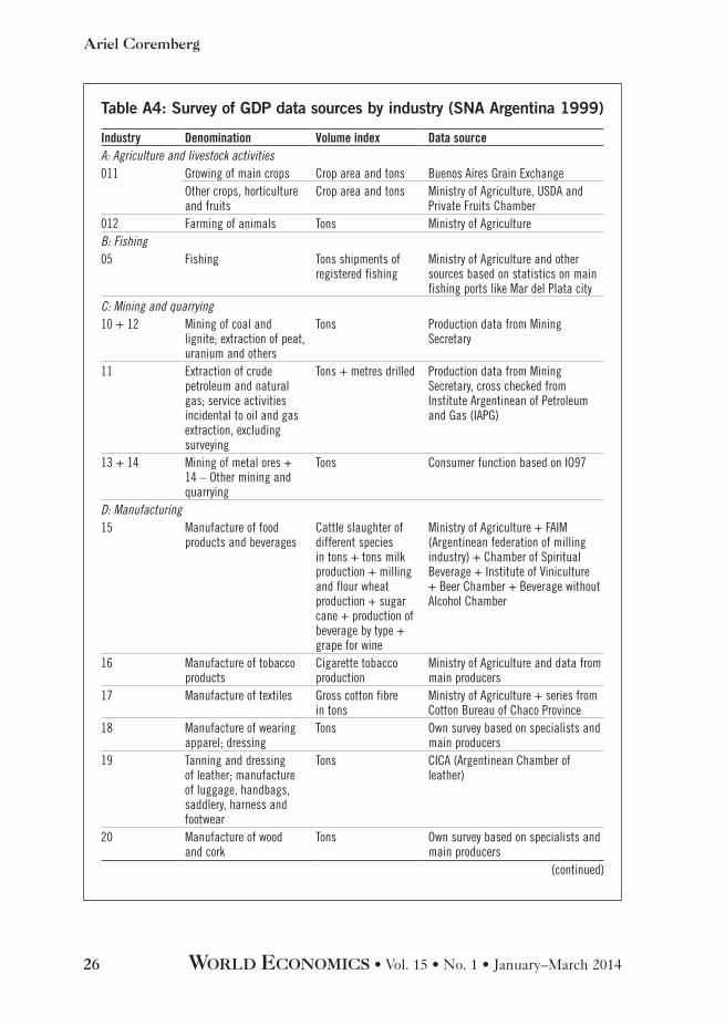
by deflating the value of production or value added at current prices (see Table A4 in the Appendix). This methodology was adopted more than two decades ago, and has been applied to the main basic series constitut-ing the GDP of Argentina. These volume index indicators do not belong to INDEC, but mainly to other more representative public and private surveys carried out by different institutions. Checking the consistency of actual GDP estimations against official GDP data is therefore possible, but a difficult task that demands time as well as a detailed knowledge of the data sources and the methodology used for estimating the GDP figures.

In order to do that checking, we reproduce the GDP of Argentina follow-ing the traditional methodology followed by National Accounts. We com-piled published and public series, which make up every industry’s value added volume index of GDP at the 4–5 digit of the ISIC classification from 1993 up to the present. The series are mostly the same taken into account by the Standard National Accounts according to the published methodol-ogy (SNA Argentina 1999), as cited in Table A2 in the Appendix.

Reproducing Argentina’s GDP: main results

We collected and compiled the same basic industry series, which in total constitute the GDP of Argentina according to published and public indicators before the 2007 statistics intervention, and we applied the traditional methodology to aggregate them.

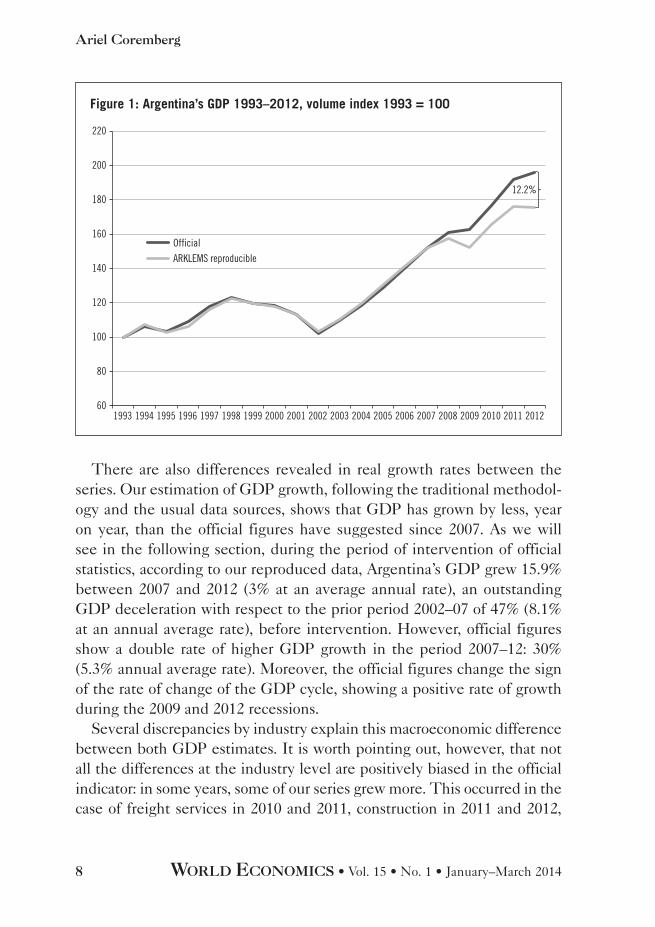
The main result of this procedure is a reproducible GDP series that replicates almost exactly official Argentine GDP growth from 1993 to 2007. After that latter year, however, an important gap appears. This gap accumulates into a substantial difference increasing every year since then, as illustrated in Figure 1.

Official real GDP shows a positive gap of 12.2% for 2012 with respect to reproducible ARKLEMS GDP. This lower level of GDP at constant prices has several implications for mac-roeconomic analyses. Argentina, in fact, has had a more modest growth profile than official data have suggested, as will be ana-lysed in the next section, but also a lower level of non-price competitiveness due to lower capitalisation, and both labour and total factor productivity.

Official real GDP shows a positive gap of 12.2% for 2012 with respect to reproduced GDP by the author.


Ariel Coremberg

There are also differences revealed in real growth rates between the series. Our estimation of GDP growth, following the traditional methodol-ogy and the usual data sources, shows that GDP has grown by less, year on year, than the official figures have suggested since 2007. As we will see in the following section, during the period of intervention of official statistics, according to our reproduced data, Argentina’s GDP grew 15.9% between 2007 and 2012 (3% at an average annual rate), an outstanding GDP deceleration with respect to the prior period 2002–07 of 47% (8.1% at an annual average rate), before intervention. However, official figures show a double rate of higher GDP growth in the period 2007–12: 30% (5.3% annual average rate). Moreover, the official figures change the sign of the rate of change of the GDP cycle, showing a positive rate of growth during the 2009 and 2012 recessions.

Several discrepancies by industry explain this macroeconomic difference between both GDP estimates. It is worth pointing out, however, that not all the differences at the industry level are positively biased in the official indicator: in some years, some of our series grew more. This occurred in the case of freight services in 2010 and 2011, construction in 2011 and 2012,

Figure 1: Argentina’s GDP 1993–2012, volume index 1993 = 100

60

80

100

120

140

160

180

200

220

1993 1994 1995 1996 1997 1998 1999 2000 2001 2002 2003 2004 2005 2006 2007 2008 2009 2010 2011 2012

OfficialARKLEMS reproducible

12.2%



and public administration during the whole period under analysis. This fact shows that our indicator does not create a systematic bias downwards in the level of the GDP, as opposed to the bias generated by the discretional intervention on the official series. Hence, the gap between the two series is mainly due to the withdrawal of the traditional methodology followed in constructing National Accounts in Argentina since the last quarter of 2007.

We compile the same series and apply the traditional methodology as historical national accounts (Table A4 in the Appendix) by industry at the 4–5 ISIC level classification. This procedure reveals the existence of a ‘Pandora’s Box’ effect of accumulation of positive gaps between official GDP series by industry with respect to our indicator. This bias occurs in most individual series (with very few exceptions). This is discussed in the following paragraphs, where we review each sector separately.

Agriculture and livestock

We reproduced this sector at a highly detailed level. We detected that some regional crops and minor livestock activities are no longer included in the official series, but this does not cause any important difference

Figure 2: Argentina GDP growth 2007–2012, annual rates

8.4%

6.3%

1.0%

8.6% 8.6%

2.2%

7.9%

4.1%

–3.1%

8.7%

6.2%

–0.4%

–0.04

–0.02

0

0.02

0.04

0.06

0.08

0.1

2007 2008 2009 2010 2011 2012

Official ARKLEMS reproducible


Ariel Coremberg

with our ARKLEMS estimation (except for a higher variance related to ‘weather effects’ and changes in supply decisions).

Mining

In Argentina, this industry is mostly based on oil and gas extraction (which represents nearly 98% of the Argentine mining sector). We also included metallic production and other mining activities but, taking into account the crisis in oil and gas production that has been ongoing in Argentina since 2000 up to the present, we captured a negative downward trend in the series, which is not reflected by its official counterpart. There is also some evidence that official series include metallic mineral extraction activities at 2004 prices instead of the 1993 base year. This is an incorrect discretionary criterion probably driven by the intention to show a positive growth trend to avoid any reflection of the crisis in oil and gas production.

Electricity, gas and water supply

The official series since the end of 2007 do not reflect the underlying trends that appear in the basic series of the main utility supply indicators.

Manufacturing sector

This sector is a core element in the construction of estimates of GDP of the National Accounts. This is due not only to its direct impact on aggregate GDP (more than 20% of the total at constant prices) but also to the indirect impact on the estimation of other sectors’ value added. This is, for example, the case for trade and transport, whose GDP estimation is directly linked to the manufacturing sector (also it represents another 10% of total GDP).

For the manufacturing sector we compiled original indicators for more than 100 different industries at 4–5 ISIC digits (representative branch), detecting any important gaps since the last quarter of 2007. Our guess is that the official series now takes into account the original INDEC Manufacturing Quarterly Survey, which collects value-of-production data at current prices, and deflates it using the wholesale index prices. As described above, the wholesale price index has been distorted since 2008. This survey has never been taken glob-ally into account in the estimation of value added and gross output of the manufacturing sector in national accounts (ECLAC 1991; SNA Argentina 1999). Using a methodology that takes into account the basic volume series of traditional Argentina national accounts, and not a manufacturing survey



that deflates values at current prices, we find very different figures in our manufacturing sector estimations.

Construction

The traditional methodology measures value added and output as a weighted compounded indicator that takes into account a volume index of construction materials12 and employment. Several years ago (before the political interven-tion), the materials’ indicators methodology was modified: the weights were changed from 1993 to 1997. The basic series have several methodological problems (e.g. cement changed from an output volume indicator to an indi-cator that captures sales to the domestic market). Since 2008, the materials’ indicator was changed and the indicator for the employment in the construc-tion sector was included in national accounts without a clear and systematic methodology. We think that the INDEC should capture total employment from a household survey, but this survey is available only with a lag of several months, so there is no reported evidence about what kind of employment indicator is in fact used in the measurement of national accounts. The GDP series elaborated by us takes into account registered employment and an indicator of materials from the main materials producers (which correlates well with the original INDEC indicator up to 2007). Important differences in the performance of the sector were also detected in 2008 and 2009.

Wholesale and retail trade

There has been a systematic gap between reproducible GDP and official GDP since 2007–08, due to the impact of the application of an adjusted series from agricultural and livestock sector and also from manufacturing.

Hotels and restaurants

There has also been a systematic gap between the two series since 2007–08 in this sector. The case of hotels and restaurants is impressive, especially during 2009: the official INDEC GDP series does not take into account the impact of the H1N1 flu and the negative shock of the international crisis on tourism activity, reflected in the basic series elaborated by the Argentine Department of Tourism. For example, room nights dropped more than 30% at a national level (50% in Buenos Aires city), and most restaurants and

12 It is called ISAC and is a Laspeyres index of cement, iron rods, paintwork, bricks and asphalt.


Ariel Coremberg

cafeterias had to close for several months due to H1N1 restrictions during that year. Nevertheless, the official GDP indicator for tourism grew by 1% (in comparison to a reduction of 4% in our alternative indicator).

Transport and communications

In this sector, there is also a systematic gap due to the impact of the application of commodity flows on adjusted series from agricultural and livestock sector and manufacturing. Our series grew more than the official series during 2010 and 2011, but since 2012 have grown less. The official GDP sector indicator does not take into account the important negative impact of labour union riots on bus and metro transport, and the accident that occurred on the main railroad passenger service on February 2012, which provoked a huge fall in passenger transport activity.

Financial intermediation

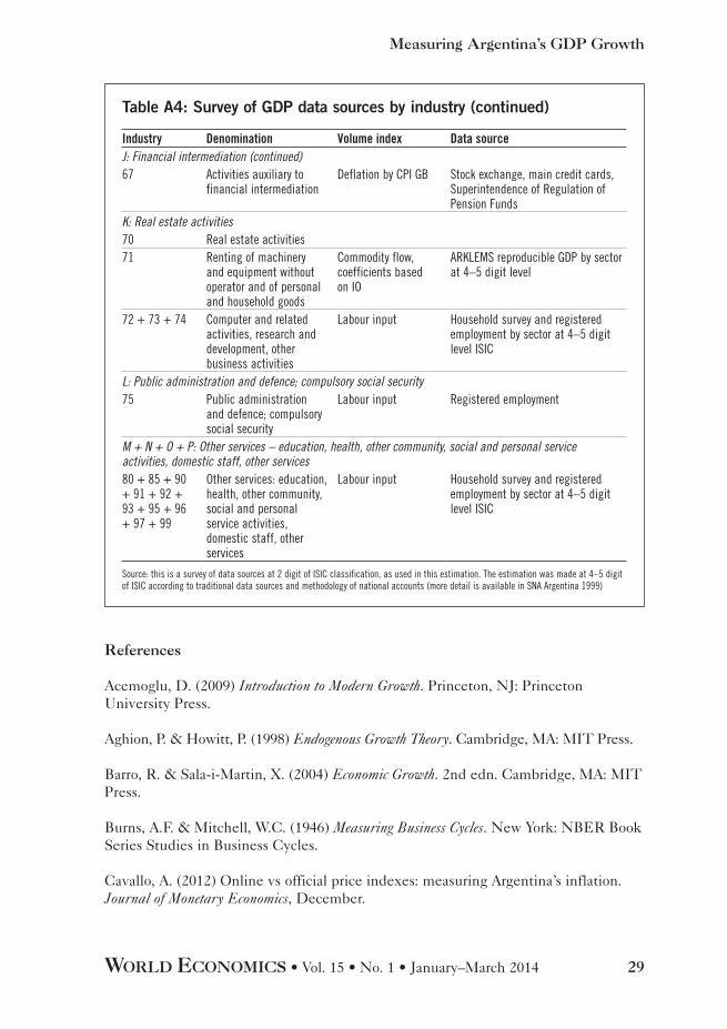
There has been a systematic gap since 2007 and this is the only case inves-tigated where the gap has to do with the deflation of nominal figures by a biased CPI: FSIM,13 bank fees and other activities related to financial intermediation such as insurance, credit cards, private pension fund fees, etc. Besides, the official GDP measurement did not take into account the drop in 2008 in the activity of private pension funds due to nationalisation.

Business and real estate activities

Once again, there has been a systematic gap between the two series since 2007–08. Some evidence of non-systematic approaches on real estate activities with own or leased property prior to intervention also exists, but this does not impact considerably on the sector’s output at 1 ISIC digit. The gap is generated because of inconsistent official measurement through commodity flows of minor sectors such as renting equipment, and incon-sistencies with the original labour input series of professional services.

Public administration

This is the only case where our GDP indicator shows a small positive gap in levels and a moderate growth against the official series, especially since 2007. The official estimation includes a non-public non-reported series

13 Financial intermediation services indirectly measured.



of public administration employment, which supposedly includes labour in public offices at the national, provincial and local levels, together with military employment. Our estimate takes into account registered employ-ment in public administration from fiscal records. This series has the disadvantage of excluding some provinces, but reflects a higher trend of public employment that is not reflected in the national accounts official non-public series. There is strong evidence of a boom in public employ-ment since 2007, and mainly during national election years (2009 and 2011), which is not totally reflected in the official national accounts.

Other services

This sector includes education, health and other services whose original methodology in the annual official series is based on the school enrolment, and hospital and other health centres utilisation indicators. But these indica-tors are not used at the required frequency; quarterly official series follows the employment series14 until 2007. We detected that the original traditional employment basic series included in our GDP estimations didn’t match the official series from 2008 producing a systematic positive bias.

Stylised facts and myths

Political interference in the production of statistics and a general recogni-tion of this problem by academia, the media and public opinion has cre-ated a number of stylised facts about economic growth in Argentina that, on closer inspection, turn out to be myths. These myths can be dispelled using our GDP estimations. Three myths are evaluated below, which we call the methodology myth, Argentina’s resurrection myth and the myth that Argentina is a Latin American growth champion.

The methodology myth: official Argentine GDP data have a positive bias upwards because official INDEC estimation deflates value added at current prices with a manipulated consumer price index

As shown above, official GDP shows a positive bias of 12.2% for 2012 compared to reproducible GDP. Since 94% of the value of GDP before

14 It is worth mentioning that the National Accounts Bureau has not published any annual revision since 1999.


Ariel Coremberg

considering the impact of political intervention is based on volume indi-cators by industry, this means that positive biases in official GDP are not due to a consistent application of a new methodology with distorted price indices, but, worse, to the act of withdrawing the traditional methodology of National Accounts and applying discretionary non-reported criteria. The reproducible GDP revision shows that, using traditional methodology and data sources, only financial intermediation (5% of GDP) is affected by deflation.15

Furthermore analysing the contribution of each sector’s value added finds that financial intermediation explains only 27.9% of the total GDP gap between official and reproducible GDP as is shown in Figure 3.

The largest sectors explaining the total gap, besides financial inter-mediation, are trade (28%) and manufacturing (22%), which explain 50% of the total gap. The rest of services and goods production explains

a smaller share compensated by minor negative gaps from public administration and agriculture.

To summarise, our GDP esti-mations show that the resulting

GDP gap does not depend on official CPI index manipulation, but is mainly due to discretionary intervention in individual industries that imply changing the original national accounts methodology.

The resurrection myth: the recent Argentine GDP growth episode was the highest growth acceleration for many decades

It is important to analyse the GDP cycle to study whether an economy is recovering from a recession or a previous crisis, and whether it restarts a process of growth acceleration. It is also useful to assess whether an econ-omy is growing in the long term beyond a cyclical recovery (Hausmann et al. 2005). This is an old and basic approach, sometimes known as the ‘NBER approach’.16 Its origins date back to a book by Burns and Mitchell (1946) written more than 60 years ago.

15 In the case of restaurants and non-regular passenger transportation, the traditional methodology uses a demand function approach (because there are no direct surveys on those industries), so index prices do not enter directly in the estimation unless through the relative prices of those categories in the CPI. But this methodology was abandoned in 2003, before the beginning of the intervention, based on a unitary income elasticity.16 National Bureau of Economic Research.

The GDP gap depends not on inflation data manipulation

but on changing the original national accounts methodology.



According to Hausmann et al. (2005) the output recovery after a crisis (‘the recovery effect’) could be sustainable in the long term as long as the post-growth output exceeds its pre-episode peak. Generally, GDP peaks coincide with an output level near the potential output, where all pro-duction factors are fully utilised. In general, GDP between cyclical peaks grows at a lower rate than during a recovery phase, because it is more difficult to grow when there is full capacity utilisation. Furthermore, GDP growth rates in the long term (between peaks) are usually lower than GDP growth rates during recoveries, because the former are based on productivity rises and not on changes in the production factors’ uti-lisation rates, as explained by Coremberg (2012a) and Jorgenson (2011).

One of the stylised facts of the commodity price boom that took place between 2002 and 2011 is that the economic growth of Latin America and Argentina occurred after a deep economic depression during the period 1998–2001. How much of the economic growth was really due to the boom and how much was due to a ‘recovery effect’? By how much did GDP

Figure 3: Industry contribution to Argentina’s GDP gap (ratio between official GDP and ARKLEMS reproducible GDP 2012 level – total GDP 2007–2012, gap level = 100% (12.2%)

–1.6

–0.7

0.0

0.5

0.7

0.7

2.3

4.5

8.2

9.0

20.4

27.9

28.0

–5 0 5 10 15

%

20 25 30

Public administration

Agriculture and livestock

Fishing

Transport and communication

Mining and quarrying

Electricity, gas and water supply

Construction

Hotels and restaurants

Real estate and other business services

Other services

Manufacturing

Financial intermediation

Trade

Accumulated GDP gap = 100% (official/reproducible)Total goods production: 23%Total services: 77%


Ariel Coremberg

accelerate, in comparison to the previous positive phase that occurred dur-ing the so-called ‘Washington Consensus period’ in the 1990s? We believe that the answers to these questions depend on the consistency of the GDP series used.

The periods of analysis have been chosen in order to compare the actual boom to that which took place during 1990–98. This period corresponds to the initial positive phase of the reforms put into force after the lost decade of the 1980s. It lasted until the negative shock of 1998 followed by the economic depression period of 1998–2002. Moreover, comparing the crisis phase of 1998–2002 to the following decade, 2002–12, allows an analysis of the impact of the present boom of commodity prices on the recovery after the crisis. We also report data for the periods 2002–07 and for 2007–12, tak-ing into account that 2007 is not technically a cyclical peak, but rather is the year when the political manipulation of official statistics began (espe-cially in the final quarter of that year.

Table 1 shows the GDP performance in the periods previously defined above according to the official INDEC statistics and to our alternative GDP ARKLEMS reproducible estimations.

Measured at annual average growth rates, the most recent growth epi-sode from 2002 to 2012 measured by reproducible GDP is similar to the previous positive phase in Argentine history from 1990 to 1998. However, the official figures show that average annual growth in the recent growth episode is stronger by 1.0% than in the previous one. Therefore, the fig-ures in Table 1 show that there was no GDP acceleration for the period 2002–12 in comparison with the previous positive cycle, 1990–98.

The official and the reproducible GDP estimates show ‘Chinese rates’ of approximately 8% annual growth, only during the period 2002–07 (or 48.3% and 47.6% accumulated, respectively). However, between 2007 and 2012, the reproducible GDP series shows that Argentina suffered a signifi-cant GDP slowdown: 15.9% in accumulated growth (or 3.0% at an annual average rate). The official GDP performance, however, is almost double at an accumulated 29.4% (or a 5.3% annual average rate).

A more formal approach to see if a growth episode qualifies as sus-tainable acceleration is that proposed by Hausmann et al. (2005). This approach classifies growth acceleration episodes and long-term growth in the long term, taking into account GDP per capita instead of GDP, using the following method:



1. gt,t+n >3.5% per annum → Growth is rapid2. ∆gt,n >2.0% per annum → Growth accelerates3. yt+n > max(yi), i ≤ t → Post-growth output exceeds pre-episode peak4. Relevant time horizon is eight years (i.e. n = 7)

where gt,t+n is the growth rate of GDP per capita (y) from t to t + n; ∆gt,n = gt,t+n − gt−n,t or the change in the growth rate at time t is simply the change in the growth over horizon n and yt+n is GDP per capita after the growth horizon.

Table 2 shows the corresponding values for g and ∆g according to the official and alternative GDP estimations.

By comparing the figures that appear in Table 2, it is evident from the reproducible data series that there was no GDP per capita acceleration for the period 2002–12 in comparison with the previous positive cycle of 1990–98. The acceleration occurs only during a period of five years (2002–07), but it does not fulfil all of Hausmann et al.’s (2005) rules for qualifying as a sus-tainable growth episode. Moreover, after 2007, the so-called ‘Chinese rates’ could not be sustained, since both GDP and GDP per capita growth showed a strong slowdown. There is no structural change on the GDP trend either, especially when we compare the trend of GDP per capita between 2002 and 2012, and the one that corresponds to the period 1990–98.

However, this technical classification of macroeconomic data does not deal with the important ‘quality’ differences of the present decade in

Table 1: Argentina GDP growth (1993 prices)

ARKLEMS (%) Official (%)1990–1998 Accumulated growth 56.3 56.3

Annual growth 5.7 5.72002–2012 Accumulated growth 71.1 91.9




Annual growth 2.5 3.4

Source: ARKLEMS; GDP growth at producer prices


Ariel Coremberg

comparison with 1990–98: more job creation, a real wages recovery and the scope of the ‘social safety nets’ in the Argentine economy. The sustain-ability of these changes in the long term, however, has been put into ques-tion. As demonstrated by Coremberg (2011, 2012a), Argentina’s growth profile showed an unsustainable growth from the point of view of source of growth: the growth profile was extensively based on factor utilisation and accumulation, while total factor productivity slowed down during the recent growth episode. As shown previously, the reason is not only unsus-tainable use and the inefficiency of the use of productive factors, but also lower growth performance that it is not recognised in official statistics.

Argentine GDP grew only 2.5% between cyclical peaks according to ARKLEMS estimation (instead of the official figure of 3.4%). One of the main lemmas of the canonical economic growth theory as pointed out by Barro and Sala-i-Martin (2004), Aghion and Howitt (1998) and Acemoglu (2009) is that ‘small numbers matter’: one point of difference of GDP growth can explain a great part of the accumulated differences in GDP per capita level between poor and rich countries in the long term. Argentina can be taken as an example of this lemma: the PPP GDP per capita of 1998 was US$8,273,17 so if the country could grow at a rate of 3.4% for the next 100 years its GDP per capita would reach US$53,559 (6.5 times its initial

17 Measured in 2000 constant price dollars.

Table 2: Argentina GDP per capita growth (1993 prices)

g ∆gARKLEMS (%) Official (%) ARKLEMS (%) Official (%)

1990–1998 Accumulated growth 43.7Annual growth 4.2

2002–2012 Accumulated growth 48.3 38.3 –0.2 1.0Annual growth 4.0 5.2

2002–2007 Accumulated growth 37.7 38.3Annual growth 6.6 6.7 2.4 2.5

2007–2012 Accumulated growth 7.7 20.4Annual growth 1.5 3.8 –2.7 –0.5

1998–2012 Accumulated growth 15.6 29.9Annual growth 1.0 1.8

Source: ARKLEMS; GDP growth at producer prices



GDP per capita level). However, if the growth rate were equal to 2.5%, as our ARKLEMS estimation suggests, then GDP per capita will reach only US$23,115, just 2.8 times the initial level. Of course, the exercise of meas-uring future GDP per capita according to official GDP growth computes ‘freaky numbers’: GDP per capita level could be 53 times higher (official figures of 2002–12) or 600 times using Chinese unsustainable rates (official figures for 2002–07). It is worth pointing out that 2.5% GDP growth and 1.0% GDP per capita growth is nearly what the Argentine growth profile was during the period 1900–2012, according to our estimates.18

The growth championship myth: Argentina is the Latin American country that has had the highest growth acceleration in the region during the last decade

We have already seen that reproducible Argentine GDP growth during the boom from 2002 to 2012 was 71% in accumulated growth, or 5.6% at an average annual rate. This performance can be compared with that regis-tered by other Latin American countries, as shown in Figure 4.

Argentina, Peru and Uruguay are the countries that lead the ranking of accumulated growth, far beyond the regional average for Latin America. The largest countries in the continent (Brazil and Mexico) grew below the region’s trend. According to official figures, Argentina is the ‘growth champion’ in the whole region: its growth accumulated an impressive 99%, which is more than double the region’s average. However, if we use our ARKLEMS GDP estimation instead, the growth performance of Argentina is substantially lower (71%, nearly 30 points less than the official figures), and lies behind those of Peru and Uruguay.

Although Latin America seems to have experienced a significant eco-nomic growth process since 2002, it is important to remember that the region was recovering from a previous economic recession. If one com-pares Latin American growth during 2002–12 (3.8% at an annual average) to the previous growth cycle of 1990–98 (3.4%), the region does not seem to show a differentiated performance between both periods. Even more, if

18 ARKLEMS Tornquist estimations measuring output including composition effects according to a growth accounting and productivity approach show a slightly lower trend of 2.3% between peaks (1998–2012) so GDP per capita would have grown in a century to US$18,206 per capita, which is 2.2 times the initial GDP per capita level (see Coremberg (2012a) for ARKLEMS Source of Growth methodology). Coremberg et al. (2007), conversely, show a GDP growth annual rate of 2.5% between 1950 and 2006. This figure updated would reach nearly 3% if we consider the whole 1900–2012 period.


Ariel Coremberg

one takes into account the period in which the regime of import substitu-tion was in force (1950–80), then Latin America grew at an annual rate of 5.5%. This figure is close to the present growth rates of most Southeast Asian countries (Ocampo 2012).

The beginning of the commodity price boom in 2002 coincided with the end of the great economic depression that had affected Latin America and began in 1998, with large currency devaluations in Brazil and Russia. The crisis was later magnified by so-called ‘flight to quality’ effect during the dotcom crises in the United States, when there was important capital flight outside Latin America. During this period of economic depression from 1998–2002, Latin America grew at an annual rate of only 1.3%, but it is worth pointing out that, while the rest of the region showed average positive but slower growth rates during that period, as shown in Figure 5, Argentina and Uruguay showed an impressive net drop in GDP, followed by Venezuela and Paraguay.

One of the reasons for the depth of the Argentine crisis was a lack of flexibility and the poor ability of its economy to face external shocks due

Figure 4: Latin America’s GDP growth, 2002–2012 (compound rate, %)

Source: ARKLEMS, ECLAC

28.0

42.1

46.0

49.0

54.6

55.0

57.7

58.8

60.6

71.1

77.4

87.2

99.1

0 20 40 60 80 100 120

Mexico

Brazil

Latin America

Paraguay

Bolivia

Chile

Colombia

Venezuela

Ecuador

Argentina ARKLEMS

Uruguay

Peru

Argentina Official



to the strong commitment to the currency exchange rate that the ‘convert-ibility law’ implied (the 1 to 1 parity between the Argentine peso and the US dollar). Similarly, Uruguay faced immediate negative consequences as a result of the crisis at the end of the convertibility law period in Argentina, because of the high interdependence between the two economies.

However, as shown above, Argentina displayed an important resurrec-tion. The exit from the crisis and the recovery of the Argentine economy were due not only to the bailout and the strong devaluation of the domestic currency at the beginning of 2002, but also to the impact of an agricultural product prices increase (especially soybean and corn), which generated a significant increase in exports. In addition, there were also significant wealth effects based on urban real estate and farming land revaluation, which in addition to a bailout helped reduce the financial vulnerability of the private corporate sector (Coremberg 2012b).

However, according to the ARKLEMS measurement, the Argentine GDP recovery was important, but its rate was similar to the one registered in the previous recovery from hyperinflation during the 1980s. According to economic growth theory, we should be able to identify the sustainability of the present growth phase if we can analyse how much of this growth

Figure 5: Latin America’s GDP growth, 1998–2002 (cumulative rate, %)

11.4

9.5

9.3

8.8

7.3

6.8

6.4

2.8

–2.9

–8.1

–17.7

–18.4

–20 –15 –10 –5 0 5 10 15

Mexico

Chile

Peru

Brazil

Bolivia

Ecuador

Latin America

Colombia

Paraguay

Venezuela

Uruguay

Argentina



Ariel Coremberg

is due to a recovery effect and how much has been based on sustainable growth above the maximum GDP level attained by the region before the crisis of 1998. When we look at that, we see that the countries’ growth

ranking substantially changes. Latin America as a whole grew 55% between 1998 and 2012 (which implies a 3.2% annual rate). However, Peru, Ecuador, Chile, Bolivia, Colombia and

Brazil experienced a growth rate that was above the regional average. Argentina’s official GDP also shows a performance above the average of the region, but if we take into account the ARKLEMS reproducible GDP measurement, then Argentina belongs to the group of countries whose growth performance is below the region’s average.

According to our figures, Argentina grew 42% between 1998 and 2012 (20% less than the official figures), and this figure is smaller than those that correspond to Brazil, Uruguay, Paraguay and Venezuela. So Argentina is the lowest growth country of Latin America in the long run.

Figure 6: Latin America’s GDP growth, 1998–2012 (compound rate, %)


42.6

42.2

44.8

45.9

46.0

54.6

55.4

62.0

62.5

65.9

69.7

71.6

104.6

0 20 40 60 80 100 120

Mexico

Argentina ARKLEMS

Paraguay

Venezuela

Uruguay

Brazil

Latin America

Colombia

Argentina Official

Bolivia

Chile

Ecuador

Peru

Argentina grew 42% between 1998 and 2012 (20% less than

the official figures), a rate slower than Brazil, Uruguay,

Paraguay and Venezuela.



These comparative performances allow us to look at another concept that is generally forgotten about in the theory of economic growth: con-tinuous growth. Not only are recovery and growth acceleration important, but also rates of growth must be continuous and sustained. This considera-tion reinforces the need to analyse continuous long-term growth periods without cyclical effects. In conclusion, the impact of the commodity price boom on Argentina allowed a recovery of aggregate demand with respect to that of the crisis period, but this has not been translated into any change in long-term growth trends. Argentina’s recent growth episode, therefore, is a case of normal recovery in terms of the country’s economic history of volatility and irregular growth, which does not seem to have generated a structural change in its long-term growth pattern.

Conclusions

This paper reports on an exhaustive revision of the Argentina National Accounts methodology in order to reproduce GDP series since 1993, and check economic growth after political interventions in the production of official statistics. GDP is estimated using the same traditional series and methodology that had been employed for 25 years up to the intervention of the official statistics in 2007. Our series reproduces Argentina’s GDP growth closely from 1993 up to 2006. Since then, the difference between the official series and ARKLEMS reproducible series accumulates a large positive bias upwards due to intervention.

The divergence between our results and official figures is due to the withdrawal of the traditional GDP measurement methodology in almost every sector of GDP. This paper shows that these distortions are not based on deflating value added by industry at current prices levels with manipu-lated price indices but mainly on discretional intervention in every indus-try component of the GDP, not only in the financial sector but also trade and manufacturing, and the rest of services and goods production sectors, with the objective to be to show a higher GDP growth.

The official series present a picture of GDP growing at higher rates during the recent recovery period (2003–12) than in the previous one (1990–98), and they make Argentina lead the GDP performance of the region. But our research demonstrates that the ARKLEMS reproducible GDP for the recent growth episode had a similar performance to that in


Ariel Coremberg

the previous positive cycle, 1990–98. Technical analyses based on typical National Bureau for Economic Research (NBER) cycle decomposition, updated by Hausmann et al. (2005), shows that Argentina does not have a sustainable growth acceleration.

This paper has shown that Argentina’s recent growth episode 2002–2012 was similar to the previous positive growth cycle period 1990–1998. Argentina was not the growth champion of the Latin America region dur-ing the recent growth episode. Argentina also has some of the highest GDP volatility in the whole region, showing the lowest GDP growth of the region in the long run, less than Brazil and Mexico, when the com-parison is realised between the peaks of the economic cycle (1998–2012). Argentine official GDP could not evade the so-called ‘Pandora’s Box’ effects, caused by the political intervention in official statistics.

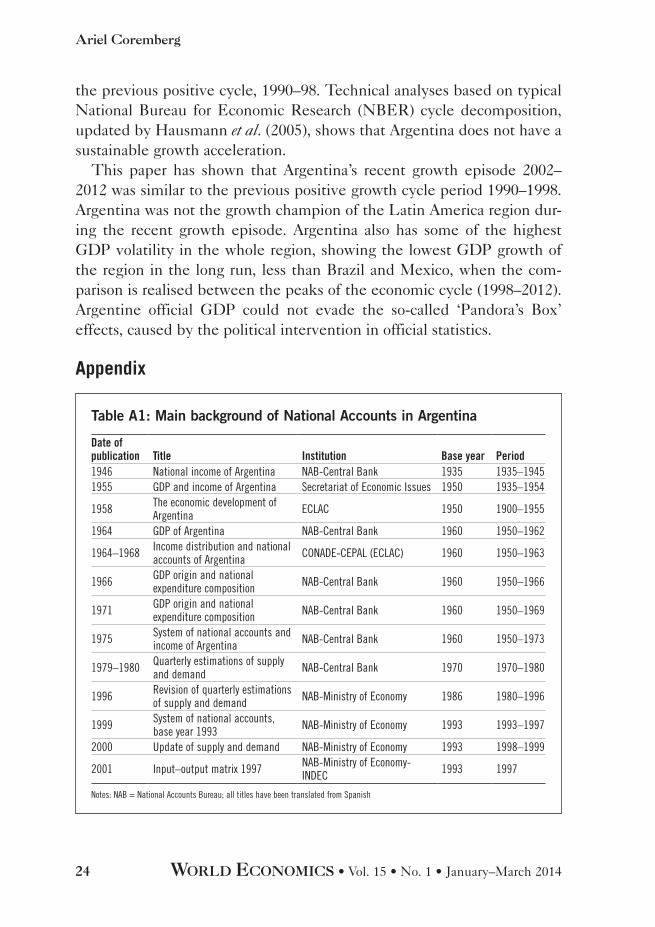
Appendix

Table A1: Main background of National Accounts in Argentina

Date of publication Title Institution Base year Period1946 National income of Argentina NAB-Central Bank 1935 1935–19451955 GDP and income of Argentina Secretariat of Economic Issues 1950 1935–1954

1958 The economic development of Argentina ECLAC 1950 1900–1955

1964 GDP of Argentina NAB-Central Bank 1960 1950–1962

1964–1968 Income distribution and national accounts of Argentina CONADE-CEPAL (ECLAC) 1960 1950–1963

1966 GDP origin and national expenditure composition NAB-Central Bank 1960 1950–1966

1971 GDP origin and national expenditure composition NAB-Central Bank 1960 1950–1969

1975 System of national accounts and income of Argentina NAB-Central Bank 1960 1950–1973

1979–1980 Quarterly estimations of supply and demand NAB-Central Bank 1970 1970–1980

1996 Revision of quarterly estimations of supply and demand NAB-Ministry of Economy 1986 1980–1996

1999 System of national accounts, base year 1993 NAB-Ministry of Economy 1993 1993–1997

2000 Update of supply and demand NAB-Ministry of Economy 1993 1998–1999

2001 Input–output matrix 1997 NAB-Ministry of Economy-INDEC 1993 1997

Notes: NAB = National Accounts Bureau; all titles have been translated from Spanish



Table A2: Author’s estimation of Argentina ARKLEMS reproducible GDP by sector, 2006–2012 (GDP in million pesos at 1993 prices)

2006 2007 2008 2009 2010 2011 2012Agriculture and livestock 17,265 18,515 18,823 14,819 19,392 20,031 17,618Fishing 497 465 484 427 472 511 502Mining and quarrying 5,219 5,162 5,090 4,911 4,932 4,737 4,636Manufacturing 54,975 59,153 60,997 58,081 63,983 66,888 65,522Electricity, gas and water supply 9,023 9,468 9,796 9,698 10,100 10,604 11,067

Construction 20,751 23,118 23,402 21,355 22,596 24,828 24,372Trade 41,587 46,222 48,457 45,037 50,677 54,603 52,462Hotels and restaurants 8,079 8,650 8,802 8,404 8,973 9,364 9,216Transport and communication 33,049 37,561 40,991 42,858 49,233 55,388 56,571

Financial intermediation 14,573 16,794 16,855 15,302 16,184 17,994 18,745Real estate and other business services 43,959 45,992 48,336 48,062 49,608 51,436 52,190

Public administration 15,561 15,957 16,758 17,917 18,762 19,781 20,799Other services 44,603 46,541 48,459 49,556 50,727 52,173 53,025Total 309,140 333,599 347,251 336,426 365,639 388,337 386,725

Source: Author’s estimation of ARKLEMS reproducible GDP by sector based on data source cited in Table A4

Table A3: Official estimation of Argentina GDP by sector, 2006–2012 (GDP in million pesos at 1993 prices)

2006 2007 2008 2009 2010 2011 2012Agriculture and livestock 17,265 19,037 18,523 15,601 20,046 19,557 17,342Fishing 497 465 484 427 472 511 502Mining and quarrying 5,219 5,195 5,250 5,193 5,113 4,933 4,980Manufacturing 54,975 59,153 61,842 61,503 67,547 74,962 74,660Electricity, gas and water supply 9,023 9,541 9,863 9,954 10,567 11,049 11,583

Construction 20,751 22,806 23,641 22,744 23,915 26,085 25,396Trade 41,587 46,219 49,870 49,751 56,245 64,486 65,739Hotels and restaurants 8,079 8,745 9,417 9,486 10,180 10,964 11,137Transport and communication 33,049 37,568 42,129 44,860 49,605 54,231 56,918

Financial intermediation 14,573 17,280 20,279 20,436 22,225 26,944 32,211Real estate and other business services 43,959 46,018 48,902 50,878 52,982 55,661 55,860

Public administration 15,561 16,134 16,758 17,609 18,486 19,220 20,008Other services 44,603 47,050 49,519 51,540 53,513 55,776 57,404Total 309,140 335,211 356,478 359,983 390,896 424,380 433,740

Source: National Statistics and Census Institute (INDEC)


Ariel Coremberg

Table A4: Survey of GDP data sources by industry (SNA Argentina 1999)

Industry Denomination Volume index Data sourceA: Agriculture and livestock activities011 Growing of main crops Crop area and tons Buenos Aires Grain Exchange

Other crops, horticulture and fruits

Crop area and tons Ministry of Agriculture, USDA and Private Fruits Chamber

012 Farming of animals Tons Ministry of AgricultureB: Fishing05 Fishing Tons shipments of

registered fishingMinistry of Agriculture and other sources based on statistics on main fishing ports like Mar del Plata city

C: Mining and quarrying10 + 12 Mining of coal and

lignite; extraction of peat, uranium and others

Tons Production data from Mining Secretary

11 Extraction of crude petroleum and natural gas; service activities incidental to oil and gas extraction, excluding surveying

Tons + metres drilled Production data from Mining Secretary, cross checked from Institute Argentinean of Petroleum and Gas (IAPG)

13 + 14 Mining of metal ores + 14 – Other mining and quarrying

Tons Consumer function based on IO97

D: Manufacturing15 Manufacture of food

products and beveragesCattle slaughter of different species in tons + tons milk production + milling and flour wheat production + sugar cane + production of beverage by type + grape for wine

Ministry of Agriculture + FAIM (Argentinean federation of milling industry) + Chamber of Spiritual Beverage + Institute of Viniculture + Beer Chamber + Beverage without Alcohol Chamber

16 Manufacture of tobacco products

Cigarette tobacco production

Ministry of Agriculture and data from main producers

17 Manufacture of textiles Gross cotton fibre in tons

Ministry of Agriculture + series from Cotton Bureau of Chaco Province

18 Manufacture of wearing apparel; dressing

Tons Own survey based on specialists and main producers

19 Tanning and dressing of leather; manufacture of luggage, handbags, saddlery, harness and footwear

Tons CICA (Argentinean Chamber of leather)

20 Manufacture of wood and cork


(continued)



Industry Denomination Volume index Data sourceD: Manufacturing (continued)21 Manufacture of paper

and paper productsTons Pulp and paper manufacturing

chamber22 Publishing, printing and

reproduction of recorded media


23 Manufacture of coke, refined petroleum products and nuclear fuel

Tons Energy Secretariat

24 Manufacture of chemicals and chemical products

Tons CIFIM, CILFA, Petrochemical Institute, Fertilizer and Agricultural Health Chamber,

25 Manufacture of rubber and plastics products

Tons Rubber Chamber

26 Manufacture of other non-metallic mineral products

Tons Own survey on main glass producers, Cement Association, Tyre Chamber

27 + 28 Manufacture of basic metals and metal products

Tons Centre of Iron and Steel Manufacturers, Aluminium Main producer

29 + 30 + 32 + 33

Manufacture of machinery and equipment, computers, communication and medical, other

Tons CAFMA, AFAT (private chambers on agricultural equipment) + Manufacturers Association of Tools Machines + own survey based on specialists and main producers

34 Manufacture of motor vehicles, trailers and semi-trailers

Tons ADEFA (Chamber of Manufactures of Vehicles)

35 + 36 + 37 Manufacture of other transport equipment + furniture + recycling, others


E: Electricity, gas and water supply40 + 41 Electricity, gas, steam

and hot water supply + water

M3 + kw + ton (water)

Secretary of Energy, Aysa (water supply), CAMMESA (electricity distribution), ENARGAS (gas regulator)

F: Construction45 Construction Weighted average

of labour input and materials indicator

Own indicator of main materials from main producers: weighted average of main materials as painting, bricks, cement, and others + labour input based on household survey and registered employment surveys

(continued)

Table A4: Survey of GDP data sources by industry (continued)


Ariel Coremberg

Industry Denomination Volume index Data sourceG: Trade50 + 51 + 52 Wholesale and retail

trade; repair of motor vehicles, motorcycles, and personal and household goods

Commodity flow on domestic production net of exports + imports by good type based on coefficients of IO

Own estimation based on own estimation of domestic production net of exports + imports (international trade data from Custom House) at 4–5 digit ISIC industry level

H: Hotels and restaurants55 Hotels and restaurants Room nights for

hotels + demand function for restaurants

Room nights (Survey of Tourism Secretariat) + restaurants: consumer demand estimated on Household Consumer Survey and flows of goods and services by type based on own estimation of income at constant prices ARKLEMS reproducible GDP net of non-market sectors at 4–5 digit ISIC

I: Transport, storage and communications61 Land transport; transport

via pipelinesPassengers by transport mode + tons for cargo transport by mode

CNRT (National Commission of Transport Regulation), National Bureau of Aero Transport

62 + 63 Air + water transport Passengers by transport mode + tons for cargo transport by mode

National Bureau of Aero Transport

64 Supporting and auxiliary transport activities; activities of travel agencies

Commodity flow, coefficients of IO

Based on demand activities at disaggregated level of ARKLEMS reproducible GDP at 4–5 digit ISIC

65 Post and telecomunications

Call minutes by type + postal shipments

CNC (National Commission of Telecommunications)

J: Financial intermediation65 Financial intermediation,

except insurance and pension funding

Deflation by CPI GB Publish methodology based on deflation of credits and deposits by unweighted average of CPI and WPI until intervention of National Accounts Bureau in last quarter 2007. If WPI is also distorted, as well as CPI, we adopted CPI GB, which is similar to other alternative private CPI and, more important, CPI of other provinces

66 Insurance and pension funding, except compulsory social security

Deflation by CPI GB Insurance premium according to Superintendence of Insurance activity

(continued)




References

Acemoglu, D. (2009) Introduction to Modern Growth. Princeton, NJ: Princeton University Press.

Aghion, P. & Howitt, P. (1998) Endogenous Growth Theory. Cambridge, MA: MIT Press.

Barro, R. & Sala-i-Martin, X. (2004) Economic Growth. 2nd edn. Cambridge, MA: MIT Press.

Burns, A.F. & Mitchell, W.C. (1946) Measuring Business Cycles. New York: NBER Book Series Studies in Business Cycles.

Cavallo, A. (2012) Online vs official price indexes: measuring Argentina’s inflation. Journal of Monetary Economics, December.

Industry Denomination Volume index Data sourceJ: Financial intermediation (continued)67 Activities auxiliary to

financial intermediationDeflation by CPI GB Stock exchange, main credit cards,

Superintendence of Regulation of Pension Funds

K: Real estate activities70 Real estate activities71 Renting of machinery

and equipment without operator and of personal and household goods

Commodity flow, coefficients based on IO

ARKLEMS reproducible GDP by sector at 4–5 digit level

72 + 73 + 74 Computer and related activities, research and development, other business activities

Labour input Household survey and registered employment by sector at 4–5 digit level ISIC

L: Public administration and defence; compulsory social security75 Public administration

and defence; compulsory social security

Labour input Registered employment

M + N + O + P: Other services – education, health, other community, social and personal service activities, domestic staff, other services80 + 85 + 90 + 91 + 92 + 93 + 95 + 96 + 97 + 99

Other services: education, health, other community, social and personal service activities, domestic staff, other services

Labour input Household survey and registered employment by sector at 4–5 digit level ISIC

Source: this is a survey of data sources at 2 digit of ISIC classification, as used in this estimation. The estimation was made at 4–5 digit of ISIC according to traditional data sources and methodology of national accounts (more detail is available in SNA Argentina 1999)



Ariel Coremberg

Chen, V., Gupta, A., Therrien, A., Levanon, G. & van Ark, B. (2010) Recent productivity developments in the world economy: an overview from the conference board total economy database. International Productivity Monitor, 19, Spring.

Coremberg, A. (2009) Measuring source of growth of an unstable economy: Argentina: productivity and productive factors by asset type and industry. Methods and Series (in Spanish). ECLAC Buenos Aires Office. Estudios y Perspectivas 41.

Coremberg, A. (2011) The Argentine productivity slowdown. The challenges after global financial collapse. World Economics, 12, 4. Available online at: http://www.world-economics-journal.com/Contents/ArticleOverview.aspx?ID=481.

Coremberg, A. (2012a) Measuring productivity in land rich economies. ARKLEMS+LAND Project, WorldKLEMS 2nd Conference, Harvard University.

Coremberg (2012b) Where is the wealth of Argentina? The national balance sheet of unstable and natural resource dependent economy. International Association of Research in Income and Wealth Conference, Boston.

Coremberg, A., Heymann, D., Goldzier, P. & Ramos, A. (2007) Patterns of saving and growth of Argentina 1950–2006. Cepal Santiago.

Cortázar, R. & Marshall, J. (1980) Índice de Precios al Consumidor en Chile: 1970–78. Colección Estudios 4, Cieplan.

Cortázar, R. & Meller, P. (1987) Los dos Chile y las estadísticas oficiales: una versión didáctica. Apuntes 67, Cieplan.

Diewert, W. & Fox, K. (1999) Can measurement error explain the productivity paradox? Canadian Journal of Economics, 32, 2, Special Issue on Service Sector Productivity and the Productivity Paradox, April, pp. 251–280.

ECLAC (1991) Revision of National Accounts and Income Distribution of Argentina. Proyecto Revisión de las Cuentas Nacionales y de la Distribución del Ingreso. Final report. ECLAC Buenos Aires. December.

EUKLEMS (2007) EU KLEMS growth and productivity accounts. Prepared by Timmer, M., van Moergastel, T., Stuivenwold, E., Ypma, G., O’Mahony, M. & Kangasniemi. M. Available online at: http://www.euklems.net.

García, J. & Freyhoffer, H. (1970) La tasa efectiva de inflación en Chile entre 1961 y 1968 y el comportamiento de los agentes económicos. Publicación 118, Instituto de Economía y Planificación, Universidad de Chile.

Hausmann, R., Prichett, L. & Rodrik, D. (2005) Growth accelerations. Journal of Economic Growth, 10, 4, December, pp. 303–329.



IO97 Argentina (2001) Input output matrix 1997 Argentina. Matriz Insumo Producto Argentina 1997. Ministerio de Economía-Secretaría de Programación Económica. Instituto Nacional de Estadísticas y Censos. Ministry of Economy-INDEC.

Jorgenson, D. (2011) Innovation and productivity growth. American Journal of Agricultural Economics, 93, 2, April, pp. 276–296.

Jorgenson, D. & Vu, M. (2001) Productivity Growth in China, 1981–95. Cambridge, MA: Kennedy School of Government.

Maddison, A. & Wu, H. (2008) Measuring China’s economic performance. World Economics, 9, 2, April–June.

Ocampo, J.A. (2012) Let’s be clear: this will not be Latin America’s decade. VoxLACEA. Available online at: http://vox.lacea.org/?q=JoseAntonioOcampo1.

OECD (2001) OECD Productivity Manual: A Guide to the Measurement of Industry-level and Aggregate Productivity Growth. Paris: OECD.

PNUD-BIRF (1992) Studies for design of public policies, national accounts methodological report. Estudio para el Diseño de Políticas Públicas. Tomo 11. Cuentas Nacionales. Informe Metodológico. United Nations Development Program – International Bank for Reconstruction and Development. Buenos Aires.

Ren, R. (1997) China’s economic performance in an international perspective. OECD Development Centre Studies.

SNA Argentina (1999) National accounts system of Argentina. Base year 1993. Quarterly and Annual Series. Ministry of Economy.

Streb, J. (2010) Why citizens tolerate the distortion of the CPI? Colectivo Economico (blog in Spanish, Argentina). Available online at: http://colectivoeconomico.org/2011/03/15/por-que-la-ciudadania-tolera-la-distorsion-del-ipc/#more-515.

Sturgess, B. (2010) Greek economic statistics: a decade of deceit. So how come the rating agencies missed it again? World Economics, 11, 2, April–June.

Young, A. (2000) Gold into base metals: productivity growth in the People’s Republic of China during the Reform Period. Mimeo, University of Chicago.

Measuring Argentina’s GDP Growth - ARKLEMS · inflation and GDP, have been subject to political...

Documents

Transcript of Measuring Argentina’s GDP Growth - ARKLEMS · inflation and GDP, have been subject to political...