FIEF Working Paper Series 2001 ISSN 1651-0852

No. 174

Measures of Technology and the Business Cycle: Evidence from Sweden and the U.S.*

by

Annika Alexius† and Mikael Carlsson††

Abstract Empirical evidence on the cyclical behavior of technology shocks, or the relative importance of technology shocks versus other structural shocks as sources of fluctuations, hinges crucially on the identification of technological changes. In this paper, we study different measures of technology in order to find out (i) to what extent they capture the same underlying phenomenon and (ii) whether the impli-cations for macroeconomic theory vary between the approaches. Several variations of the production function approach and structural VAR models are investigated: the classic Solow residual, the refined Solow residuals of Burnside et al (1995) and Basu and Kimball (1997), large cointegrated VAR models as in King et al (1991) and a small VAR in first differences á la Galí (1999). It turns out that the different measures of technological change are reasonably coherent when applied to US data. However, they are often insignificantly related in the case of Sweden. Furthermore, our results do not support the hypothesis that business cycle fluctuations are primarily driven by changes in technology. Keywords: Technology shocks; Production function approach; Structural VAR models JEL classification: C32; D24; E32 November 15, 2001 _______________________________________________________ *We would like to thank seminar participants at FIEF and Örebro University for helpful

comments and suggestions, and Lennart Berg and Jon Samuels for help with preparing the data.

†Trade Union Institute for Economic Research, SE-111 24 Stockholm, Sweden.

Tel: +46 8 6969915. Fax: +46 8 207313. E-mail: annika.alexius@fief.se ††

Department of Economics, Uppsala University, Box 513, SE-751 20 Uppsala, Sweden. Tel: +46 18 4711129. Fax: +46 18 4711478. E-mail: mikael.carlsson@nek.uu.se .

1 Introduction

The identification of technological change is a crucial element of several areas

of macroeconomics. For example, evidence on the relationship between technol-

ogy shocks and business cycle variables may be used to evaluate the empirical

relevance of different classes of business cycle models. RBC models predict that

hours worked should be positively related to technology shocks, whereas models

emphasizing e.g. price rigidities generally predict a negative contemporane-

ous relationship (see e.g. Basu, Fernald and Kimball (1998) and Galí (2000)).

In recent empirical studies, the contemporaneous response of hours worked to

technology improvements is found to be negative.1

The empirical relevance of different classes of business cycle models can also

be evaluated using structural VAR models. Variance decompositions provide in-

formation about what shocks that have caused the fluctuations in real output at

business cycle frequencies. A finding that technology shocks dominate the cycli-

cal fluctuations of real output can be interpreted as empirical support for RBC

models, while a finding that monetary shocks are more important constitutes

evidence against them.

As all structural shocks, technology shocks are inherently unobservable. Ev-

idence on the relationship between technology shocks and business cycle vari-

ables, or the relative importance of supply versus demand shocks, is therefore

conditioned on the particular method used to identify the technology shocks.

In this paper, we study different measures of technological change in order to

answer two questions: To what extent are the different methods for identifying

technology shocks capturing the same phenomenon? Do the resulting technol-

ogy shocks have similar relationships to business cycle variables such as real

output growth and hours worked, or is the empirical support for e.g. RBC

models a function of the approach used to identify technological change?

The two main techniques used for identifying technology shocks are struc-

tural VAR models and the production function approach. There are consid-1 See e.g. Galí (1999), Kiley (1998), Basu et al. (1998) and Carlsson (2000).

2

erable methodological differences within each category. King, Plosser, Stock

and Watson (1991), Galí (1999) and others impose restrictions on the long-

run effects of shocks within structural VAR models to distinguish technology

shocks from other sources of fluctuations. King et al. (1991) estimate a six-

variable VAR including real output, consumption, investment, the real money

supply, nominal interest rates and inflation. Technology shocks are identified

using the assumption that no other structural shock affects real output in the

long-run. Galí (1999) focuses on a small two-variable VAR model of changes

in labor productivity and hours worked. He separates technology shocks from

non-technology shocks by assuming that only the former have long-run effects

on labor productivity.

Long-run restrictions on VAR models have been used to identify structural

shocks within various fields. Examples are Blanchard and Quah (1989) and King

et al. (1991) for real output, Dolado and Jimeno (1997) for unemployment,

Wehinger (2000) for inflation, and Clarida and Galí (1994) for real exchange

rates. These studies produce conclusions like ”technology shocks cause about

40 percent of the variability of real output at business cycle frequencies” or ”the

bulk of the long-run movements in real exchange rates are due to real demand

shocks”.

Conclusions from VAR studies about the sources of fluctuations in various

variables has had considerable effects on the direction taken by subsequent the-

oretical research. A relevant question is then to what extent structural VAR

models actually capture e.g. true technology shocks. This issue has frequently

been debated but not systematically studied empirically. Stockman (1994) and

Kiley (1998) question the clear-cut distinction between supply shocks and de-

mand shocks, according to which demand shocks do not affect real output in the

long run. They argue that demand shocks can affect real output in the long run,

for instance by inducing a larger capital stock. The use of long-run restrictions

to identify structural shocks has also been questioned by e.g. Faust and Leeper

(1997). Among all, they argue that different types of ”true” shocks can only

be aggregated into a single structural category if they have the same effect on

3

the endogenous variables. King et al. (1991) and Rogers (1999) demonstrate

that the number of variables included in the VAR has a major effect on the

conclusions in terms of variance decompositions. In King et al, the share of

technology shocks on the three-year forecast error variance of output falls from

70 to 40 percent when two nominal variables are added to the VAR. Similarly,

Rogers shows that real demand shocks appear less important to movements in

real exchange rate when more variables are included in the model.

An obvious problem when discussing the VAR approach to identifying dif-

ferent types of shocks is that since structural shocks are unobservable, there

exists no true measure against which the outcome of the VARs can be evalu-

ated. Clarida and Galí (1994) use what they call ”a duck test” to check the

validity of their identification scheme. They plot the demand shocks identified

by their VAR model and discuss whether it is possible to detect the major de-

mand related events of the sample period in the graph. In the words of Clarida

and Galí (1994), ”if it walks like a duck and quacks like a duck, it must be a

duck”. However, technology shocks differ from other structural shocks in the

sense that there exist well-established alternative methods for identifying them.

The most popular approach is variations of the Solow (1957) residual.

Solow (1957) identifies technological change as the residual from a produc-

tion function, taking increases in production factors into account. His orig-

inal method requires perfect competition, constant returns to scale and full

factor utilization. Since deviations from these assumptions introduce cyclical

non-technology related variation, the Solow residual is not likely to be a good

measure of technology at the business cycle frequency. Instead, we rely on the

refinements of Solow’s original method developed in Hall (1988, 1999), Burn-

side, Eichenbaum and Rebelo (1995) and Basu and Kimball (1997) which allows

for these assumptions to be relaxed.

A few authors provide correlations between the technology shocks identified

by their VAR models and some other measure of technology. For instance, King

et al. (1991) report a correlation of 0.48 between their measure and the Solow

residual of Prescott (1986). However, the procedure used by Prescott (1986) is

4

not likely to provide robust estimates of technology movements at business cycle

frequencies since it does not take the phenomena listed above into consideration.

The correlation with the refined Solow residual of Hall (1988), who corrects for

increasing returns to scale and imperfect competition but not for variable factor

utilization, is only 0.19. Furthermore, Kiley (1998) calculate correlations be-

tween his VAR technology shocks and the extended Solow residuals of Basu and

Kimball (1997) and Burnside et al. (1995) for 17 American industries. About

half of the correlations are significantly positive and the cross industry average

is 0.22. These studies compare technology shocks from different approaches for

particular sample periods, and industries in the case of Kiley, but they do not

investigate the concordance of the methods given that they are actually supplied

with identical information.

In this paper, several different methods for identifying technology shocks are

applied to the same data sets. We use the classic Solow residual, the Burnside

et al. (1995) and the Basu and Kimball (1997) approaches using data on en-

ergy and hours per employee, respectively, to correct for factor utilization, large

structural VAR models a’la King et al. (1991) and a small structural VAR as

in Galí (1999). The production function approach requires disaggregate data

(see e.g. Basu and Fernald (1997)), whereas large VAR models are estimated

using aggregate data where variables like the money supply can be assumed

to be endogenous. We study four different data sets consisting of disaggregate

industry observations and aggregate macrodata for the United States and Swe-

den. The purpose of the exercise is two-fold. First, we want to compare the

different measures of technology with each other to investigate whether they

capture the same unobservable phenomenon. Do long-run restrictions on VAR

models produce technology shocks resembling those identified by the production

function approach? Moreover, it is interesting to compare U.S. results to the

results from an small open economy, such as the Swedish. For example, when

applying the production function approach on data for a small open economy

we can use instruments that are not likely to be neither valid nor relevant for

the U.S. economy. Second, because the empirical relationship between technol-

5

ogy on one hand and e.g. labor input on the other can be used to distinguish

between business cycle models, we investigate whether the technology shocks

captured by these different approaches have similar relationships to these other

variables. If the implications for macroeconomic theory are similar across differ-

ent measures of technology, the differences between them are less consequential

than if, for instance, the empirical support for RBC models is a function of the

method used to capture technology shocks.

The paper is organized as follows. Section 2 discusses the data. Section

3 outlines the different approaches to identifying technology shocks, method-

specific estimation considerations and aggregation issues. Section 4 compares

the results for the different approaches. Section 5 discusses the robustness of

the results and section 6 concludes.

2 The Data

We use four different data sets in this paper: quarterly observations on aggregate

data and an disaggregate industry data set on annual frequency for both the U.S.

and Sweden. The reason for using two aggregation levels is that the production

function approach requires disaggregate data (see e.g. Basu and Fernald (1997)),

whereas the large VARs model focus on the endogenous interaction between

macroeconomic aggregates.

The disaggregate U.S. data set is compiled by Dale Jorgenson and Barbara

Fraumeni and consists of a panel of 33 U.S. industries covering the entire U.S.

non-farm private economy for the period 1948 to 1991. Various versions of this

data set has been widely used, e.g. by Basu et al. (1998) and Basu and Fernald

(2001) and is described in detail in Jorgenson, Gollop and Fraumeni (1987).

For comparability with the former two references we focus on the sample period

1950-1989. The Swedish disaggregate data set covers the Swedish non-farm

private economy and is divided into 15 industries (see the data appendix for

all details).2 For the disaggregated Swedish data we use the sample 1968-1993.2 In a closely related paper Carlsson (2000) analyze a subset of this data set, i.e. the

6

The aggregate U.S. data set covers the period 1948:1-1989:4 and are collected

from the BEA, the BLS and the Federal Reserve Board of Governors. The

aggregate Swedish data set is collected from Statistics Sweden and covers the

period 1970:1-1993:4.

The methods used in this paper to estimate technology growth can all be

viewed as decompositions of output, or labor productivity (output/hours) in the

Galí (1999) model, into a technology driven component and a component driven

by other factors. Thus, to make the comparison of technology measures across

aggregation levels and methods meaningful we need to use consistent measures of

output and hours across the data sets. To this end, we use the same population

on both the aggregate and the disaggregate level for output and hours, i.e. the

non-farm private economy. Moreover, the (small) remaining discrepancies are

corrected by adjusting the quarterly observation in the aggregate data set so

that they sum up to the annual observation in the disaggregate data set in each

year.3

3 Identification of Technology Shocks

The two main methods for identifying technology shocks studied here are the

production function approach and structural VAR models. Three baseline VAR

models are used, the six-variable model of King et al. (1991), a Scandinavian

version of the King et al. model and the two-variable model of Galí (1999).

Technology growth can also be estimated as the residuals from a reduced

form production function. This methodology was pioneered by Solow (1957).

Subsequent research has extended Solow’s approach to allow for a variety of

phenomena that are likely to introduce non-technology related cyclical variation

into the technology measure. In addition to the Solow residual, we use the

specifications of Burnside et al. (1995) and Basu et al. (1998), which differ from

manufacturing industries.3 The value of these constants is close to one, i.e. within the range 0.96 to 1.02 in the

Swedish data and 0.92 to 1.09 in the U.S. data. Thus, the remaining differences before thecorrection are small.

7

each other in how cyclical factor utilization is handled.

3.1 The VAR Approach

A measure of technological change can be extracted from structural VAR mod-

els by imposing restrictions on the long-run effects of the structural shocks.

The models of King et al. (1991) and Galí (1999) represent two different em-

pirical strategies. Galí (1999) focuses on the (stationary) first differences of

labor productivity and hours worked within a two-variable VAR. King et al.

(1991) estimate a large, cointegrated VAR with six I(1) variables (real output,

consumption, investment, real money balances, the nominal interest rate and

inflation). We also consider a Scandinavian version of the large VAR model

which treats inflation and money growth as stationary variables.

The idea to use restrictions on the long run effects to identify structural

shocks is due to Blanchard and Quah (1989). King et al. (1991) and Galí (1999)

present theoretical models to motivate their identifying restrictions. However,

the formulation of the long run restrictions is remarkably similar across VAR

studies. Monetary shocks are identified using the long-run neutrality of money,

i.e. by assuming that they have no long-run effect on real variables. Technology

shocks are assumed to be the sole driving force of real output (labor productivity

in the Galí specification) in the long run. In our large VAR models with un-

restricted estimates of the cointegrating vectors, monetary shocks are actually

allowed to affect investment and consumption, but not output, in the long run.

The parameters capturing the effects of monetary shocks on consumption and

investment are however small and often insignificant. In most cases, the restric-

tion that they are either zero or equal with opposite signs for the two nominal

variables is not rejected. All restrictions on the cointegrating space hence imply

that the monetary shocks do not affect investment and consumption in the long

run. The exact formulation of the identifying restrictions differs between the

two VAR specifications.

8

3.1.1 A large VAR-model a’la King et al. (1991)

King et al. (1991) estimate a six variable VAR containing output, y, consump-

tion, c, investment, i, real money balances (m− p), a nominal interest rate, R,and inflation, ∆p, where lower case letters denote the log of the variable and ∆

is the first difference operator. We follow their six variable approach both for

the U.S. and the Swedish aggregate data sets.4

We start with the following n-variable cointegrated VAR:

∆zt = µ+Πzt−1 +pXi=1

Γi∆zt−i + ξt, (1)

where zt = [y, c, i, (m− p), R,∆p]0, µ is a vector of drift terms, Π and Γ arecoefficient matrices and ξt is a vector of white noise disturbances. The existence

of long-run equilibrium relationships (cointegration) among the variables implies

that the system is driven by a reduced number of common stochastic trends.

Common trends models can be analyzed using the framework developed by King

et al. (1991) and refined by Warne (1993) and others. The cointegrated VAR in

(1) can be rewritten as a common trends model (see e.g. Hylleberg and Mizon

(1989)):

zt = z0 + φ (L) vt +Θτ t, (2)

where

τ t = µ+ τ t−1 + ϕt. (3)

Here, z0 denotes a vector of initial conditions, vt is a vector of white noise

disturbances and φ (L) is a matrix lag polynomial. The term φ (L) vt constitutes

the transitory component of zt. The number of cointegrated vectors, r, in (1)

determines the number of independent stochastic trends k in the common trends

model (2) as k = n − r. The stochastic trends are denoted τ t, which is a k-

dimensional vector of random walks with drift µ and innovations ϕt. Thus, the

I(1) component of zt is described by the term Θτ t, where the loading matrix Θ4 Note that our U.S. data set differ somewhat from what King et al. (1991) use.

9

determines how the endogenous variables are affected by the permanent shocks

ϕt in the long run. The permanent shocks are also included in vt, which allows

them to affect the transitory component of zt.

For exact identification of the k structural shocks in ϕt, we need to impose

k(k−1)/2 restrictions (see e.g. Warne (1993)). Economic theory frequently hasimplications that can be translated into restrictions on the loading matrix Θ, the

cointegrating rank of the system and/or the parameter values in the cointegrat-

ing vectors. For instance, the balanced growth conditions imply that the ratios

of consumption to output and investment to output should be constant in the

long run. Consumption and investment should then be cointegrated with out-

put and the parameters in the cointegrating vector should be [1,−1]. Anotherexample is monetary neutrality. If money is neutral in the long run, monetary

shocks only affect nominal variables. The parameters in Θ that capture effects

of monetary shocks on real variables should than be zero.

We estimate the King et al. (1991) specification for Swedish and US ag-

gregate quarterly data. The number of lags p is determined using information

criteria (Akaike, Schwarz, Hannan-Quinn), but chosen sufficiently high to re-

move residual autocorrelation as indicated by the LM test for first and fourth

order autocorrelation, and the multivariate Portmanteau test. We use four lags

in our baseline model for Sweden and two lags for the United States. As up to

six lags can be included in the former case, and up to four lags in the latter, we

also estimate these alternative models to study the robustness of the results.

The main features of the King et al. (1991) specifications, the cointegrat-

ing rank and hence the number of stochastic trends are consistent with their

findings. The cointegrating rank is investigated using the Johansen (1991) mul-

tivariate maximum likelihood approach (see Table 1). There are three cointe-

grating vectors, normalized as long run equilibrium relationships between (i)

consumption, output, inflation and the nominal interest rate, (ii) investment,

output, inflation and the nominal interest rate, and (iii) demand for real bal-

ances, output, inflation and the nominal interest rate.

Most of the parameters of the cointegrating vectors have the expected signs

10

and magnitudes (see Table 2). For instance, the coefficients on real output

in the long-run equilibrium relationships for consumption, investment and real

money are [-0.86, -0.61, -1.19] for the United States, and [-0.65, -2.91, -0.05]

in the case of Sweden. The restriction that these coefficients all equal unity is

rejected for Sweden but not for the United States. Other conceivable restrictions

are that the real variables are not affected by inflation and the interest rate at

all in the long run, or that they are affected only by the real interest rate.

The most restrictive restriction that is not rejected by the data for the King

specification on US data is that the coefficients on real output all equal unity

and the coefficients on inflation and the nominal interest rate are equal with

opposite signs in the two long run equilibrium relationships for consumption

and investment. The latter restriction is imposed on our U.S. baseline version

of the King model.

Following King et al. (1991), we interpret the three stochastic trends as

technology (supply), real interest rate (demand), and a nominal (monetary)

trend. Technology shocks are identified by the assumption that no other shocks

affect real output in the long run. This implies that Θ12 and Θ13 in the loading

matrix equal zero. Long-run monetary neutrality provides the third required

restriction by imposing a zero long-run effect of monetary shocks on the real

interest rate.

3.1.2 A Large Scandinavian VAR Model

The inflation rate is assumed to contain a unit root in the King et al. (1991)

specification, as are the real money supply and the nominal interest rate. For the

United States, inflation is typically considered to be I(1). However, the Swedish

inflation rate is more appropriately modelled as stationary with a shift in the

mean as the Riksbank decided to reduce inflation in the beginning of the 1990s.

Similarly, Swedish real money balances as well as the nominal interest rates is

borderline stationary (the ADF test statistics are —2.01 and -2.45, respectively).

With a mean shift dummy for the 1990s, all three series are clearly stationary,

11

as is money growth. Hence, a better specification of a large, cointegrated VAR

in the case of Sweden is to include the price level and the level of the nominal

money supply as I(1) variables.

Four to six lags can be included in the VAR depending on which informa-

tion criterion and what autocorrelation test and significance level one prefers to

rely on. We use four lags in the baseline model. The five-variable VAR model

with real output, real consumption, real investment, the nominal price level and

the level of the nominal money supply contains three cointegrating vectors (see

Table 1). We normalize the cointegrating vectors to get three long run equi-

librium relationships between (i) consumption, real output, money, and prices

(ii) investment, real output, money, and prices (iii) the nominal money supply,

the price level and real output. Economic theory implies that the consumption

output ratio, the investment/output ratio and the real money balances to out-

put ratio should be stationary. This full set of restrictions is not rejected by the

data.

The two stochastic trends are interpreted as a real technology trend and a

nominal demand trend. Only one identifying restriction is required for exact

identification. Again, we assume that only technology affects real output in the

long run, i.e. that Θ12 is zero (given zt = [yt, ct, it, mt, pt]).

In the US case, ADF tests indicates that inflation is stationary for the full

sample 1947-1989. King et al. (1991) start their sample in 1954, removing the

Korean war and price control period around 1950, which yields the standard

I(1) inflation rate. Real money balances and the nominal interest rate are

clearly I(1). Hence, the King et al. (1991) specification is more appropriate

for the United States than for Sweden. However, since the log difference of

M2 is also borderline stationary, the Scandinavian model can be applied to US

data as well. Two lags are required to remove residual autocorrelation at the

ten-percent level according to the multivariate Portmanteau test. The Johansen

(1991) trace test statistics for cointegrating rank appear in Table 1. Again, there

are three cointegrating vectors which are normalized as above.5 Here, however,5 The cointegrating rank tests are inconclusive in case of the four lag Scandinavian model

12

even the least restrictive theoretical restrictions on the cointegrating space are

rejected by the data in the US case. Hence, we estimate four Scandinavian

models for Sweden (given four and six lags, with and without restrictions on

the cointegrating space) and two for the US (with two and four lags, without

restrictions on the cointegrating space).

3.1.3 A Small VAR-model a’la Galí (1999)

Galí (1999) separates the influence of technology shocks from that of non-

technology shock within a two variable VAR-model containing the first dif-

ferences of hours worked and labor productivity. The identifying assumption

is that only technology shocks affect labor productivity in the long run. The

number of parameters that has to be estimated in the Galí specification is small,

which allows us to estimate the model also on annual industry data.

We estimate a large number of Galí specifications on three different lev-

els of aggregation for Sweden and the United States: The non-farm private

economy, the manufacturing sector and on each industry. The middle level is

added because it can be argued that the production function approach is more

appropriate for the manufacturing sector than e.g. for the service sector. In

particular, we estimate the Burnside et al. (1995) version of the Solow resid-

ual on the manufacturing industries only because energy consumption is a less

appropriate measure of capital utilization outside the manufacturing sector.

Since the log differences of hours and labor productivity are stationary, there

is no cointegration in the Galí model. The preferred number of lags is deter-

mined using information criteria and the binding condition that the residuals

should not be autocorrelated. Because different information criteria indicate

different lag structures, and there is some degree of freedom in terms of what

autocorrelation test and significance level to rely on, we estimate two alter-

native specifications on each data set. In order to obtain comparable results,

for the US. The trace tests indicate r = 4, while the λ-max test indicates no cointegration(r = 0). Since this model is only used to study the robustness of the results, we neverthelessrely on the existence of three cointegrating vectors in this case as well.

13

however, the choices of lag length are not re-optimized for each industry. For

the disaggregate industry data, the Galí model is estimated using one and four

lags. Aggregate manufacturing is a rare case of unanimous choice of lag length

as all information criteria indicate that one lag should be used and there is no

significant autocorrelation in the VAR(1) residuals. The aggregate Swedish Galí

specification requires four or five lags to remove residual autocorrelation depend-

ing on the preferred significance level. Two lags can be used in the aggregate

Galí specification for the United States as there is no significant autocorrelation

in the residuals. However, the Akaike information criterion indicates five lags

and we estimate a four lag model to study the robustness of the results with

respect to variations in the choice of lag length.

3.2 The Production Function Approach

The idea behind the production function approach is that technological change

can be measured as the residual from a production function, taking increases in

production factors into account. We start by assuming the following firm-level

production function:

Yi,t = F (Zi,tKi,t, Ei,tHi,t, Vi,t,Mi,t,Ai,t), (4)

where gross output Y is produced combining the stock of capital K, hours H,

energy V and intermediate materials (less energy)M . The firm may also adjust

the level of utilization of capital, Z, and labor, E. Finally, A is an index of

technology.

Differentiating the log of (4) with respect to time and invoking cost minimiza-

tion yields a gross output version of the standard Hall (1988, 1990) specification

generalized to allow for variable factor utilization. That is:

∆yi,t = ηi[∆xi,t +∆ui,t] +∆ai,t, (5)

where η denotes the overall returns to scale and ∆x and ∆u are cost-share-

weighted growth rates (first log differences) of observable inputs (K,H, V,M)

and utilization (Z,E), respectively. Thus, given measures of ∆yi, ∆xi, ∆ui and

14

an estimate of ηi, the resulting residual∆ai provides a times series of technology

growth for firm i. That is, the standard Solow residual purged of the effects of

increasing returns, imperfect competition and varying factor utilization.

The main empirical problem associated with (5) is that capital and labor

utilization are generally unobservable. A solution to this problem is then to

include proxies of utilization in (5). We follow the approaches of Basu and

Kimball (1997) and Burnside et al. (1995) who include hours per employee and

energy, respectively, to control for cyclical factor utilization. Although these

two specifications differ in how variation in factor utilization are handled, they

both share the basic structure of (5). Thus, the two specifications derived

below yield measures of technology that are robust to imperfect competition

and non-constant returns to scale and, under various conditions, varying factor

utilization.

3.2.1 The Basu and Kimball (1997) Specification

The first approach we consider is to use the restrictions that follow from firms’

optimal behavior to derive a relation between factor utilization and observable

variables. This is the route taken by Basu and Kimball (1997) who derives a

relationship between the growth rate of hours per employee, ∆hpe, and utiliza-

tion growth, ∆u, from the first order conditions of a dynamic cost-minimization

problem. This yields the empirical specification employed by e.g. Basu et al.

(1998), Basu and Fernald (2001) and Basu, Fernald and Shapiro (2001) to esti-

mate technology growth:

∆yi,t = αi + ηi∆bxi,t + γi∆hpei,t + εi,t, (6)

where ∆ denotes first log difference, cJ is the cost share of factor J in total costs,

∆bxt is defined as cK∆kt + cH∆ht + cV∆vt + cM∆m and ∆hpe is the growth

rate of hours per employee.6

6 Expression (6) corresponds to an assumption of (4) being a Cobb-Douglas function.Basu and Kimball (1997) also generalize their approach by including regressors to control forvariation in the rate of capital depreciation (due to varying capital utilization). However,as stated in Basu et al. (2001), ”...including these terms barely affects estimates of technicalchange”.

15

When implementing the Basu and Kimball (1997) specification, and the

Burnside et al. (1995) specification below, we follow the empirical strategy out-

lined by Basu et al. (2001). First, the specifications are regarded as log-linear

approximations around the steady state growth path, i.e. the output elasticities,

ηcJ , are treated as constants. Second, the steady state cost shares are estimated

as the time average of the cost shares. Third, when compiling the cost shares we

assume that firms make zero economic profits in the steady state.7 This allows

us to estimate the cost share of capital as a residual. Finally, the growth rate of

technology, ∆a, is modeled as a random walk with the drift α and the random

shock ². This strategy for modeling the technology process is consistent with

the assumptions underlying the structural VAR approach.

3.2.2 The Burnside et al. (1995) Specification

An alternative approach to identify factor utilization proxies is to make ad-

ditional assumptions directly about the production technology. The approach

employed by e.g. Burnside et al. (1995) employs the idea of Griliches and Jor-

genson (1967), to use energy consumption as a proxy for capital utilization.

This procedure can be legitimized by assuming that there is a zero elasticity of

substitution between energy and the flow of capital services, ZK, which implies

that energy and capital services are perfectly correlated. Adding the assump-

tion that labor utilization is constant, we arrive at the empirical specification

of Burnside et al. (1995):8

∆yi,t = αi + ηi∆exi,t + εi,t, (7)

where input growth ∆ext is defined as (cK+cV )∆vt+cH∆ht+cM∆mt.9 Energy

is however only likely to be a good proxy for the utilization of heavy equipment.7 For U.S. evidence in favor of this assumption see the discussion in Rotemberg and Wood-

ford (1995). For the industries 1 to 9 in the disaggregate Swedish data set we have datato estimate economic profits. Our data implies a time average (1968-1993) for the share ofeconomic profits in the aggregate revenues for these industries of -0.001.

8 Note that the term energy is used in a broad sense in this section. In fact, Burnsideet al. (1995) used electricity consumption as proxy for capital utilization. We will return tothe exact definition of energy that we use in the empirical work when we discuss the data.

9 In Burnside et al. (1995) time varying cost shares are used. Equation (7) rests, however,on the assumption that F (ZK,EH,V,M,A) =

©ASα1 (EL)α2Mα3 , S = min[ZK,V ]

ª, where

16

This specification is therefore less appropriate outside the manufacturing sector.

Since the Burnside et al specification relies on a different set of assumptions than

the Basu and Kimball specification we estimate both approaches as a robustness

test. However, we only use data from the manufacturing sector for the Burnside

et al. specification.

3.2.3 Instrumentation and Estimation

Because the firm is highly likely to consider the current state of technology when

making its input choices, instrumental variable technique are required to credi-

bly identify the residuals from the robust production function specifications as

technology growth. Appropriate instruments to avoid this endogeniety are vari-

ables that are exogenous relative to variation in technology while correlated with

economic activity. The most commonly used instruments in the literature are

variations of the so-called Hall-Ramey instruments and Federal Reserve policy

shocks derived from an identified VAR. The Hall-Ramey instruments consist of

the growth rate of the real price of oil, the growth rate of real defense spending

and a dummy variable for the political party of the president. For the U.S.

disaggregate data set we use the following instrument set: the lagged Federal

Reserve policy shock derived from an estimated reaction function of the Federal

Reserve and the lagged growth rates of the real oil price and real defense spend-

ing. This instrument set yields results that are close to the results presented by

Basu et al. (1998), Basu and Fernald (2001) and Basu et al. (2001).

Because the relevance of real defense spendings and the political dummy

variable in U.S. data has been questioned (see e.g. Wilson (2000) and refer-

ences therein), it is interesting to compare baseline U.S. result to the results

obtained from a different economic environment, allowing for other, potentially

highly relevant, instruments. The main point of studying the Swedish economy

in addition to the United States is that we can reasonably treat it as a small

E denotes the fixed level of effort. Carlsson (2000) experiment with using industrial accidentsas a proxy for effort on Swedish data. This approach does not work well and is not consideredin this paper.

17

open economy. This characteristic legitimize the use of other instruments, such

as foreign demand, as well as strengthen the validity argument for the real oil

price. Moreover, Sweden has maintained a fixed exchange rate regime, with a

small number of discrete devaluations, throughout the sampling period. Thus,

the nominal exchange rate should be a valid instrument. For the Swedish dis-

aggregate data, we use the same instrument set as in Carlsson (2000), i.e. the

current and once lagged growth rate of a foreign demand index, the first and

second lag of the growth rate of a nominal exchange rate index, the current

value of the growth rate of the real oil price and a political dummy variable (see

the data appendix for details).

Following Basu et al. (1998) and Basu and Fernald (2001) we combine in-

dustries into groups. Within each group we allow for fixed industry effect and

heterogenous returns to scale. When estimating (6) we restrict the hours per

employee parameter, γ, to be equal across industries. Each group is then esti-

mated with standard 3SLS methods using the instruments discussed above.

Both the U.S. and the Swedish industries are divided into four groups, i.e.

mining (four industries in the U. S. data/one industry in the Swedish data),

nondurables manufacturing (10/4 industries), durables manufacturing (11/4 in-

dustries) and services and others (8/6 industries). Since the U.S. input data

is divided into capital, labor, energy and other intermediate inputs we use this

broad energy measure when estimating the Burnside et al. specification on U.S.

data.

When estimating the Basu and Kimball specification on Swedish data, we

drop the hours per employee proxy for all groups except for mining and petro-

leum extraction. This is done since the hours per employee parameter is esti-

mated with the wrong sign (negative, but insignificantly so) for these groups. In

fact, hours per employee is generally acyclical in the Swedish data set, whereas

the same variable is generally strongly procyclical in our U.S. data set.10 Since10 The correlation between the growth rate of aggregate hours per employee and aggregate

output growth is -0.07 in the dissagregate Swedish data set, whereas the corresponding corre-lation for the dissagregate U.S. data set is 0.70. One explanation of the difference in cyclicalbehavior of hours per employee in the U.S. and Sweden is differences in labor institutions.

18

the inputs are divided into capital, labor, electricity and other intermediate in-

puts we use electricity consumption as the energy measure when estimating the

Burnside et al. specification on Swedish data.11

In Tables 3 and 4, we present a summary of the results from the production

function regressions. The null hypothesis of the Sargan-test of valid instruments

and a correctly specified model can not be rejected on the five-percent level in

any of the systems. Tables 3 and 4 also present relevance measures of the

instrument sets, i.e. R2:s and partial R2:s (defined as in Shea (1997)) averaged

over industries. In the U.S. case the relevance of the instruments is low and

the results are somewhat sensitive to the exact specification of the instrument

set. This problem is often encountered when estimating production functions

since it is difficult to find good instruments (see e.g. Burnside (1996) for a

discussion). The procedure outlined above yields however results that are close

to previous U.S. studies (see below). In the Swedish case the instrument set

have a quite high explanatory power for the weighted input indices and the

results are more robust to variations in the specification of the instrument set.

The lower relevance for the Swedish instrument set for hours per employee is

due to the fact that the hours per employee variable is generally acyclical in

Sweden, whereas the instrument set is designed to be relevant for the level of

economic activity.

Tables 3 and 4 presents the average of the estimated returns to scale for each

group in the U.S. and Sweden, respectively. For nondurables manufacturing,

durables manufacturing and services and others we can compare our findings

For example, the overtime premium, i.e. the markup on the base wage, was 62 percent in theSwedish manufacturing sector as compared to 43 percent in the U.S. manufacturing sector in1985. Overtime constituted 2.6 percent of total hours worked in Swedish manufacturing during1981-1992, whereas the same fraction for the U.S. manufacturing sector (calculated from BLSdata) was 8.3 percent during the same time period. The Swedish estimates are taken from (orcompiled using the data underlying) Nordström-Skans (2001). The US overtime premium iscalculated using the estimate of the share of overtime workers receiving a premium (0.865) inthe U.S. manufacturing sector presented by Trejo (1993) and by assuming that those workersthat did receive a premium received the time-and-a-half premium as mandated by the FairLabor Standards Act. In the total sample used by Trejo (1993), 95 percent of those whoreceived any type of overtime premium did in fact get the time-and-a-half premium.11 Since electricity expenditure are unavailable for industries outside mining and manufac-

turing, inputs are divided into capital, labor and intermediate inputs in these industries.

19

for the Basu and Kimball specification with the findings of Basu et al. (2001),

although they use a somewhat different time period and methodology. The

results for both the returns to scale and the hours per employee parameter

are quite similar. For the nondurables manufacturing (durables manufacturing)

[services and others], we arrive at an average point estimate of the returns to

scale of 0.69 (1.05) [0.70] and an estimate of the hours per employee parameter

of 1.69 (0.76) [0.70] as compared to 0.78 (1.03) [1.00] and 1.21 (0.74) [1.33] in

Basu et al. (2001). The Swedish manufacturing results are very similar to the

results of Carlsson (2000), who estimate both the Basu and Kimball and the

Burnside et al. specification using a slightly different empirical strategy. For

the Basu and Kimball specification we find an average of the returns to scale

point estimates for nondurables (durables) of 1.26 (1.24) as compared to 1.26

(1.30). For the Burnside et al. specification we find an average of the returns

to scale point estimates for nondurables (durables) of 1.18 (1.17) as compared

to 1.19 (1.18). Thus, overall, our estimation results are in line with previous

studies.

3.3 Aggregation

To compare the results of the different approaches to identify technology growth

we need to aggregate industry-level technology growth series from the produc-

tion function approach to aggregate technology growth. Following Basu et al.

(1998) and Basu and Fernald (2001) we define aggregate technology growth,

∆aA, as:

∆aAt =Pi ωi,t

∆ai,t1− ηi(cV,i + cM,i)

, (8)

where ωi is the industry’s share in aggregate nominal value added. The de-

nominator in (8) converts gross output technology growth to a value added

measure. This conversion allows us to compare the aggregate technology series

from the production function approach to the technology series from the struc-

tural VAR-models which are estimated using value added data. To compare

technology growth series on different frequencies, we convert quarterly series to

20

annual series by summation.

To analyze the cyclical patterns implied by the different technology measures,

we calculate correlations between the technology measures and the growth rates

of aggregate real value added, aggregate total hours worked and an aggregate

primary input index. We define aggregate real value added growth, ∆yAt , as the

first log difference of the sum of real value added across industries.12 Aggregate

total hours growth, ∆hAt , is defined as the first log difference of the sum of total

hours across industries. The aggregate primary input index is defined as:

∆xAt = cAH∆h

At + (1− cAH)∆kAt , (9)

where cAH is defined as the time average of the share of labor expenditures in

aggregate nominal value added and ∆kAt is the first log difference of the sum

of capital across industries. Given the definitions above, the aggregate Solow

residual is conveniently defined as:

SRt = ∆yAt −∆xAt . (10)

The aggregation procedure outlined above is then applied to two levels: the

non-farm private economy and the manufacturing sector.

4 Empirical Results

Although we are not aware of previous systematic studies of whether structural

VAR models capture the same technology shocks as the production function

approach, several authors calculate correlations between different measures of

technological progress. King et al. (1991) report a correlation of 0.48 between

their VAR technology shocks and the Solow residual of Prescott (1986), which

is constructed assuming constant returns to scale, perfect competition and con-

stant factor utilization. Because deviations from these assumptions introduce12 This definition of aggregate value added growth yields an almost identical measure as the

divisia definition discussed in Basu and Fernald (1995) on annual basis. Since we lack datato construct the divisia measure on quarterly frequency we use the definition above.

21

demand related procyclical noise, refined measures are preferable when ana-

lyzing the behavior of technology shocks at business cycle frequencies. The

correlation between the VAR technology shocks of King et al. (1991) and the

Solow residual of Hall (1988), which allows for increasing returns to scale but

not variable factor utilization, is only 0.19.

Kiley (1998) compares his VAR technology shocks for 17 American manu-

facturing industries to the technology measures of Basu and Kimball (1997) and

Burnside et al. (1995), i.e. the approaches for taking variable factor utilization

into account that we use. 7 of the 17 correlations are significantly positive in the

former case and 9 of 17 in the latter. The correlations are however not very high,

0.22 on average and in no case above 0.70. A problem when interpreting these

findings is that it is difficult to know just how high the correlations should be in

order to justify the conclusion that the VAR models do capture the same under-

lying phenomenon as the alternative approaches. Kiley (1998) finds his results

reassuring even though about half of the correlations are insignificant and King

et al. (1991) also consider their correlations of 0.48 and 0.19 between the VAR

technology shocks and two Solow residuals sufficiently high. King et al. (1991)

and Kiley (1998) compare technology shocks derived from different methods for

the same sample periods, and also the same industries in the latter case. We

apply the different techniques for identifying technology shocks to identical data

sets, which allows a more exact comparison of the methods.

To study whether the different methods capture the same unobservable phe-

nomenon, and whether the differences matter in the sense that different ap-

proaches lead to different conclusions about the driving forces of business cycles,

we calculate the correlations (i) between the different technology measures, and

(ii) between the technology shocks and business cycle variables. The results for

Sweden are presented in section 4.1, the results for the United States appear in

section 4.2 and industry-level evidence is presented in section 4.4. The effects

of minor variations in the specification of the VAR models and other robustness

issues are discussed in Section 5.

22

4.1 Swedish Results

Table 5 contains the results for the aggregate Swedish private non-farm econ-

omy. We compare six different technology measures: the Solow approach, the

Basu and Kimball (1997) specification with hours worked as proxy for factor

utilization, the Burnside et al. (1995) approach using energy consumption, the

large, cointegrated six variable VAR of King et al. (1991), the Scandinavian five

variable specification and the small two variable VAR of Galí (1999).

Focusing first on the relationship between the different approaches for iden-

tifying technology growth, we see that the measure from the Galí VAR model is

significantly positively related both to the Basu and Kimball measure and the

Solow residual on the five-percent level. The measures from the Scandinavian

and the King models are, however, unrelated to both the Basu and Kimball

residual and the Solow residual. Hence, only two out of six correlations be-

tween the technology measures from the two main approaches are significantly

positive and the average correlation is 0.33. The two large VAR models, the

King specification and the Scandinavian model, produce similar but not identi-

cal results in terms of technology growth. The correlation between the series is

0.71. The King model utilizes the same data on levels of output, consumption

and investment as the Scandinavian model. It is the treatment of the monetary

side of the economy differs between the two specifications. The Burnside et al.

technology measure is compiled using data from the manufacturing industries

only and can therefore not be compared to the economy-wide measures from the

large VAR models. It is however similar to the Basu and Kimball specification

as the correlation between the series amounts to 0.91.

The correlations between the cyclical variables are in line with what is ex-

pected. Output growth is strongly correlated to both input (0.78) and hours

growth (0.78). Moreover, since hours is by far the most volatile part of the

primary input index, defined in (9), the correlation between hours growth and

the input index is almost unity (0.98).

Turning to cyclical behavior of the different technology measures, it is clear

23

that we replicate the standard finding of a strongly procyclical Solow resid-

ual. The correlation between the Solow residual and output growth amounts to

0.71. The correlation between the Solow residual and hours and input growth is

also positive, although not significantly so. It has been argued that the finding

of a procyclical Solow residual is due to firms endogenous responses to demand

changes in the presence of phenomena such as imperfect competition, increasing

returns to scale and variable factor utilization rather than from truly procycli-

cal technological changes (see e.g. Basu and Fernald (2001) and the references

therein). Our application of the Basu Kimball specification to Swedish data

is robust to imperfect competition and increasing returns to scale but not to

variable factor utilization since we were forced to drop the hours per employee

variable for all groups but the mining industry. Because factor utilization is

assumed to be procyclical, leaving out hours per employee is likely to bias the

technology residual towards a positive correlation between the technology resid-

ual and output, input and hours growth. However, when studying the results

for the Basu and Kimball measure, we find that it is acyclical. The correlation

with output growth is 0.11 and insignificant. Moreover, the correlation between

the Basu and Kimball measure and input and hours growth are significantly

negative on the five-percent level, -0.49 and -0.49, respectively. The Burnside

residual which takes variable factor utilization into account through the firms’

consumption of electricity is even more countercyclical with a zero correlation

with output growth and large negative correlations with input and hours worked

(−0.65 and −0.57, respectively).An interesting finding concerning the results from the VAR models is that

the cyclical pattern of the technology measure derived from the Scandinavian

five variable VAR and the two variable VAR of Galí are very similar to that

of the Basu and Kimball and the Burnside et al. measures. The technology

measure of the Scandinavian specification is acyclical with output growth (-

0.23) and significantly negatively correlated to input (-0.44) and hours growth

(-0.45). The technology measure of the two-variable VAR of Galí is also acyclical

with output growth (-0.04), significantly negatively correlated with input growth

24

(-0.43) and negatively correlated with hours growth (-0.40) but insignificantly

so. Thus, these measures imply that technological improvements are associated

with periods of contractions in input and hours growth while output growth do

not seem to increase to any large extent, at least not contemporaneously. These

results are hard to reconcile with predictions from the standard RBC model,

whereas they are in line with the predictions of e.g. a sticky price model (see e.g.

Basu et al. (1998)). The technology measure from the King et al. specification,

which may be argued to be less appropriate than the Scandinavian specification

for Swedish data, are, however, not significantly correlated to any of the cyclical

variables. It is nevertheless interesting to see that the point estimates for the

correlations between the King et al. measure and input and hours growth are

negative (-0.07 and -0.05, respectively).

4.2 U.S. Results

The correlations between our six different technology measures for the U.S. pri-

vate non-farm economy and their relationship to cyclical variables are presented

in Table 6. A first observation from Table 6 concerns the cross correlations of

the different technology measures. All measures except the one derived from

the Galí model are significantly positively related to the Solow residual on the

five percent level. We also see that the technology measure from the Scandina-

vian model and the Galí model are positively related to the Basu and Kimball

residual on the five-percent level. The correspondence between the two main

approaches for identifying technology shocks is thus higher here than in the

Swedish case. Four out of six correlations are significantly positive and the

average correlation is 0.39.

Another encouraging finding in Table 6 is that all VAR technology measures

are significantly positively related to each other on the five percent-level. The

correlation between the King specification and the Scandinavian model is 0.72.

The correlation between the refined Solow residuals of Basu and Kimball (1997)

and Burnside et al. (1995), estimated using manufacturing data only, is 0.76.

25

Thus, the results from both the refined production function residuals and the

structural VARs seem to be robust to changes in the empirical models.

As for Swedish data, we find the expected relationships between the busi-

ness cycle variables. Input and hours growth are significantly procyclical as

the correlations with output growth are 0.66 and 0.77, respectively, and hours

growth is highly positively correlated to input growth (0.94). We also replicate

the standard finding of the Solow residual being strongly positively correlated to

output growth (0.81). Furthermore, the Solow residual is positively correlated

to hours growth (0.29) and to the input index (0.09), but insignificantly so on

the five-percent level in both cases.

When imperfect competition, increasing returns to scale, and cyclical factor

utilization are allowed, the cyclical behavior of the technology measures from

the production function approach change dramatically. The Basu and Kimball

measure is uncorrelated with output growth (0.16), while significantly negatively

related to both the input index (-0.49) and hours growth (-0.34). The Burnside

et al. energy corrected measure, which is estimated for the manufacturing in-

dustries only, is acyclical with output growth (0.20) and significantly negatively

related to input (-0.43) and hours growth (-0.34).

Table 6 also shows that all three technology series derived from the VAR:s

display a cyclical behavior that is similar to that of the refined Solow resid-

uals. The VAR technology shocks are uncorrelated to output growth on the

five-percent level, and the point estimates of the correlations between these

technology measures and input and hours growth are all negative. The corre-

lation between the Scandinavian VAR model is acyclical with output growth

(0.18) and is negatively correlated to input (-0.29) and hours growth (-0.28) but

not significantly so on the five-percent-level. We see a similar pattern for the

measure derived from the King model. The correlations between the King mea-

sure and output, input and hours growth (0.17, -0.25 and -0.23, respectively).

The Galí measure is also acyclical with output growth (0.01) and negatively

correlated with input (-0.30) and hours growth (-0.35), and significantly so on

the five-percent level in the latter case.

26

Overall, the U.S. evidence on input and hours movement in times of tech-

nology improvements are at odds with the RBC-models prediction of a positive

contemporaneous response of inputs in response to a technology improvement.

Moreover, the similarities in the cyclical behavior and the significantly positive

cross correlations between the measures of the Basu and Kimball specification,

the Scandinavian VAR and the VAR model of Galí leads us to the conclusion

that these measures reflect the same underlying unobservable phenomenon.

4.3 Robustness of the VARs

The choice of various details in the empirical specification of a VAR is rarely

self evident in the sense that there is only one possibility or even one clearly

superior alternative. Different information criteria typically produce different

optimal choices of lag length, different tests or significance levels may indicate

that different number of lags are required to remove residual autocorrelation,

restrictions on the cointegrating space can be imposed or not, and so on. We

therefore study the sensitivity of the technology shocks with respect to the minor

changes in the empirical specification.

We have estimated eight VAR models for the aggregate Swedish economy:

Two King models using four and six lags but without restrictions on the cointe-

grating space (all restrictions suggested by economic theory were rejected by the

data in this case), four Scandinavian models, also with four and six lags with

and without restrictions on the cointegrating space, and two Galí models with

four and five lags. None of the models display obvious signs of misspecification

and they are all optimal choices using at least one criterion. Table 7 shows the

results from this robustness analysis.

Changing the number of lags has a negligible influence of the technology

shocks in case of the King model and the Galí model. These two correlations are

0.91 and 0.93, respectively. For the unrestricted Scandinavian model, the effect

of adding two more lags is slightly larger as the correlation between the two sets

of technology shocks falls to 0.73. Finally, the Scandinavian model with a full

27

set of theoretical restrictions on the cointegrating space is quite sensitive to the

number of lags which is indicated by a correlation of 0.41 between the technology

measures derived from the four and the six lag versions of the model. Imposing

permissible restrictions on the cointegrating space appears to have some effect

on the results as the correlations between the Scandinavian specifications with

the same number of lags, with and without restrictions are 0.62 and 0.50.

Overall, 11 of the 28 correlations between the technology shocks from differ-

ent Swedish VAR specifications are significantly positive on the five-percent

level. The main part of the insignificant correlations are cross correlations

between variations of the Galí model and the large VAR:s. The two large,

cointegrated VAR models produce similar technology shocks except for the re-

stricted Scandinavian specification with six lags. The Swedish sample 1973-1993

is dominated by a few major monetary policy shocks, the large devaluations of

the Swedish krona in 1981 and the deep recession from 1991 to the end of the

sample which was induced by the defence of the fixed exchange rate with the

interest rate hiked up to 500 percent. If the size of the deterministic trend com-

ponent varies between the models, small differences in the extent to which the

technology trends pick up these cyclical movements has a major impact on the

results.13 The qualitative conclusions about the relation between technology

growth and cyclical variables also varies between the specifications of the VAR

models. However, in no case we find a significant positive correlation between

the technology and hours which we would expect in an RBC-world.

Table 8 shows the corresponding robustness results for eight US VARmodels:

Two King specifications with two and four lags, with and without restrictions

on the cointegrating space, the Scandinavian model with two and four lags, and

the small Galí model with three and four lags. The results in Table 8 provide

support for the conclusion that the Scandinavian and the Galí VAR models

reflect the same underlying phenomenon in US data. All cross correlations be-

tween these two measures are significantly positive. Moreover, all correlations13 Variations in the magnitude of the deterministic trend component µ has a similar effect

to varying λ in a Hodrick-Prescott filter, i.e. if µ is large relative to the variance of thetechnology shocks in ϕt, the stochastic trend become more linear.

28

between the measures from the Scandinavian and the King model are signifi-

cantly positive. The results for the correlations between the King and the Galí

measures are more mixed, five out of eight correlations are significantly positive.

Varying the number of lags in the VAR has negligible effects on the technology

shocks as the relevant correlations are above 0.88. Similarly, imposing or not

imposing permissible restrictions on the cointegrating space produces technol-

ogy shocks with correlations of 0.88 and 0.70 for the two and four variable King

specification, respectively.

The Scandinavian and the Galí models also produce similar technology mea-

sures as compared to the Basu and Kimball measure. All four correlations be-

tween these VAR measures and the production function measure from the Basu

and Kimball model are significantly positive. However, non-of the correlations

between the VAR measures derived from variations of the King model and the

Basu and Kimball measure are significantly positive. As in the Swedish case,

the qualitative conclusions about the cyclical behavior of technology growth are

sensitive to the exact specification of the VAR models, although none of the

VAR specifications implies that technology growth has an expansionary short-

run effect on hours worked.

Structural VAR models can be used to obtain Forecast Error Variance De-

compositions (FEVDs) at different horizons. Variance decompositions show how

much of the variance of a variable that stems from a certain structural shock.

At business cycle frequencies, the variance decompositions provide information

about the share of business cycle variations in real output that is caused by

technology shocks. The first column of Table 9 contain the three-year FEVDs

of output for the six different VAR models applied to aggregate Swedish data:

The King specification with four and two lags, and the Scandinavian specifica-

tion with two and four lags, with and without restrictions on the cointegrating

space. It is clear that technology shocks is a minor source of business cycle fluc-

tuations in this data set. Only 7.4 to 15.4 percent of the variations are caused

by technology shocks. While the results differ slightly between the empirical

specifications, the qualitative conclusion remains the same across the variance

29

decompositions for Swedish output growth. This can be interpreted as more

evidence against the real business cycle model, since the standard RBC-model

relies on technology shocks as the primary driving force behind business cycle

movements. Since the correlations between the Swedish VAR technology shocks

were generally to small to convincingly motivate the conclusion that the dif-

ferent specifications capture similar shocks, it is reassuring that the results in

terms of the empirical relevance of business cycle models are robust to various

permutations of the VAR models.

The share of technology shocks in the variance decomposition for US output

growth at the three-year horizon appear in the second column of Table 9. Here,

the different models yield slightly different conclusions. Five specifications ar-

rive at a relative importance of technology shocks in the range of 12.3 to 16.0

percent. The restricted King specification with four lags produce a larger share

of technology induced variations, i.e. 23.4 percent. However, these results do

not support the view that technology shocks constitute the main driving force

of business cycle variation in real output.

4.4 Evidence from industry data

In this section we study the coherence between the industry specific Basu and

Kimball residual and the technology measure from the structural VAR approach

of Galí (1999). To this end, we estimate two small VAR-models a’la Galí on

annual gross output data for each industry, using one lag and four lags for both

Sweden and the U.S. Thus, we supply the Galí model with exactly the same data

as the Basu and Kimball specification. For the manufacturing industries, the

technology measure from the Burnside et al. (1995) approach using consumption

of electricity as proxy for capital utilization are included in the analysis.

Table 10 summarizes the Swedish results from this comparison on industry

data. It also displays the number of significant correlations (on the five-percent

level) as well as the number of significant correlations with a sign opposite to

that of the average correlation. The correlation across the Galí specifications are

30

0.64 on average and all but one of the underlying correlations are significantly

positive. The correlations between the VAR technology measures of Galí and

the Basu and Kimball measure are about 0.3, with about one third of them sig-

nificant. We also present the results for the Burnside et al. specification. These

results are compiled using manufacturing data only. The Burnside measure is

highly correlated with the Basu and Kimball measure on average (0.93) with

all eight correlations significantly positive. Finally, we see that the Burnside

measure is generally uncorrelated with the Galí measures, 0.16 (one lag) and

0.21 (four lags), respectively and only one correlation is significant in the four

lag case and non in the one lag case. Thus, the coherence between the VAR and

the production function measures are quite low also when applied to Swedish

industry data.

Tables 11 presents the U.S. results from the comparison on industry data.

The average correlations between the Galí technology measures with one and

four lags and the Basu and Kimball measure are 0.55 and 0.45, with 27 and

26 out of 31 correlations significantly positive, respectively. Hence, the two

approaches for capturing technology shocks are even more similar at the indus-

try level than for aggregate data when applied to U.S. data. These results are

confirmed when turning to the Burnside measure, using energy consumption

to correct for variable factor utilization. The average correlations between the

Burnside residual and Galí measures are 0.50 and 0.40, with 17 and 14 corre-

lations out of 21 significantly positive, respectively. The coherence within each

approach is also high. The average correlation between the Basu and Kimball

and Burnside et al. series amounts to 0.83, and the average correlation between

the one and four lag measures from the Galí model is 0.78. In both cases all

underlying correlations are significantly positive. These results can be compared

to Kiley (1998) who finds a significant correlation between the Basu and Kim-

ball (Burnside) measure and the Galí measure in 7 (9) out of 17 industries and

an average correlation of 0.23 (0.22).

31

5 Conclusions

We have applied six different techniques to identify technology growth on Swedish

and US data in order to investigate whether they capture the same phenomenon

and whether the implications for macroeconomic theory are robust to the choice

of method. Our results are somewhat mixed. Above all, the US and Swedish

results differ in terms of the cohesiveness between the approaches to identify

technology growth.

For the U.S., a robust finding is that the technology measures derived from

the large Scandinavian VAR, the small VAR of Galí and the production function

approach of Basu and Kimball are significantly positively correlated to each

other. The technology measure derived from the large VAR model of King is

however not related to the Basu and Kimball residual, and the relation to the

Galí measure is not robust. The classic Solow residual is significantly correlated

with all alternative measures except for the Galí measure. Hence, the different

approaches for identifying technology shocks yield reasonably similar results

when applied to US data.

The Swedish results are more dismal. The small Galí VAR model and the

large VAR models do not yield technology series that are significantly corre-

lated. This may be due to that the Swedish sample 1973-1993 is dominated by

a few major demand related events. Small differences in the extent to which the

models identify these cyclical movements as permanent technology shocks cause

large differences in the resulting technology measures. However, the technology

measure from our baseline specifications of the Galí VAR model are significantly

correlated to comparable technology measures derived from the refined produc-

tion function approaches and to the Solow residual. The latter finding turns out

not to be robust to small variations in the baseline VAR. The Solow residual is

not related to any of the measures derived from the large VAR models in the

Swedish case.

Our U.S. industry level evidence on the relationship between technology

shocks from a structural VAR versus the production function approach can be

32

compared to the findings of Kiley (1998). About half of his correlations between

the Galí VAR measure and the Basu and Kimball (Burnside) technology mea-

sures are significantly positive and the average correlation across the industries

is only 0.23 (0.22). When controlling for differences in the data by providing

these three approaches with exactly identical information, we find that different

technology measures are much more similar. Between the Galí and the Basu and

Kimball measures 27 of 33 correlations are significantly positive, and between

the Galí and the Burnside measures 17 of 21 of the correlations are significantly

positive. The average correlations across the industries are also more than twice

as high as in Kiley (1998), 0.55 (0.50) for the Basu and Kimball (Burnside) mea-

sures. The Swedish industry evidence is, however, less encouraging. We find an

average correlation between the Galí VAR measure and the Basu and Kimball

(Burnside) measure of 0.27 (0.16), with 4 (0) out of 15 (8) of the underlying

correlations significantly positive.

We are also interested in whether variations in the specification of the struc-

tural VAR results in small or large changes in the resulting technology measures.

Again, the results differ between the two countries. For the US, all cross correla-

tions between the measures derived from the large VAR models are significantly

positive and also between the large Scandinavian VAR models and the small

Galí VAR models. The results for the correlation between the measures derived

from the large VAR models of King and the small VAR models of Galí are more

mixed, with five out of eight correlations significantly positive. Overall, the

structural VAR approach is remarkable robust in the U.S. case, both to major

and minor variations in the empirical specification. For Sweden, the correlations

between the structural VAR model are less robust.

Turning to the cyclical behavior of the technology shocks, we find similar

patterns in both the refined versions of the Solow residual as well as in the tech-

nology measures derived from the baseline structural VARs. In the Swedish case,

none of the measures derived from the refined Solow residuals or the baseline

VARs are significantly correlated to output growth and 7 of the 10 correlations

with inputs are significantly negative. In the U.S. case none of these measures

33

are significantly correlated with output, whereas 5 out of the 10 correlations with

inputs are significantly negative. Moreover, in both the Swedish and the U.S.

case the point estimates of all of the remaining insignificant correlations with

inputs are negative. Thus, the cyclical pattern that emerges is that technologi-

cal improvements are associated with periods of contractions in inputs, whereas

there is no significant (contemporaneous) increase in output. This finding can

easily be reconciled with e.g. a sticky price model (see e.g. Basu et al. (1998))

but is clearly at odds with the standard RBC-model.

Refining the standard measure of technology by allowing for phenomena

like imperfect competition, increasing returns to scale and cyclical factor uti-

lization or applying a structural VAR model hence has a radical effect on the

cyclical properties of technology growth relative to the stylized facts that re-

fer to the classic Solow residual. More specifically, the correlation with output

growth falls from about 0.75 for the classic Solow residual to about 0.15 for

the Basu and Kimball specification in both the Swedish and the US aggregate

data sets. Furthermore, the refined production function residuals are generally

significantly negatively correlated with input and hours growth. The results

from the structural VARs confirm that the refined Solow residuals constitute a

more appropriate measure of technology at business cycle frequencies since they

produce technology measures with similar cyclical behavior.

Another piece of evidence that points away from technology shocks as the

prime driving force of business cycle fluctuations is the forecast error variance de-

composition presented in the paper. Our baseline VAR models all indicate that

technology shocks account for a small and insignificant fraction of the three-year

variation of output growth, 10.4 to 16 percent, and the largest fraction observed

for all of our variations of the large VAR specifications is 23.4 percent. Overall,

the qualitative conclusions in terms of the empirical validity of different business

cycle models are more robust across our methods for identifying technological

change than the technology shocks themselves.

34

References

Basu, S. and Fernald, J.: 2001, Why Is Productivity Procyclical? Why Do We

Care?, In C. Hulten, D. Edwin and M. Harper, ed., New Developments in

Productivity Analysis, The University of Chicago Press, Chicago, IL.

Basu, S. and Fernald, J.: 1995, Are apparent productive spillovers a figment of

specification errors?, Journal of Monetary Economics 36, 165—188.

Basu, S. and Fernald, J.: 1997, Aggregate productivity and aggregate technol-

ogy, International Finance Discussion Papers No. 593, Board of Governors

of the Federal Reserve System .

Basu, S., Fernald, J. and Kimball, M.: 1998, Are technology improvements

contractionary?, International Finance Discussion Papers No. 625, Board

of Governors of the Federal Reserve System .

Basu, S., Fernald, J. and Shapiro, M.: 2001, Productivity growth in the 1990s:

Technology, utilization, or adjustment?, NBER Working Paper No 8359 .

Basu, S. and Kimball, M.: 1997, Cyclical productivity with unobserved input

variation, NBER Working Paper No 5915 .

Blanchard, O. and Quah, D.: 1989, The dynamic effects of aggregate demand

and supply disturbances, American Economic Review 79, 655—673.

Burnside, C.: 1996, Production function regressions, returns to scale and exter-

nalities, Journal of Monetary Economics 37, 177—201.

Burnside, C., Eichenbaum, M. and Rebelo, S.: 1995, Capital Utilization and

Returns to Scale, In B. Bernanke and J. Rotemberg, ed., NBER Macroeco-

nomics Annual, MIT Press, Cambridge, MA.

Carlsson, M.: 2000, Measures of technology and the short-run responses to

technology shocks: is the rbc-model consistent with swedish manufactur-

ing data?, Working Paper 2000:20, Department of Economics, Uppsala

University .

35

Clarida, R. and Galí, J.: 1994, Sources of real exchange rage fluctuations: How

important are nominal shocks?, Centre for Economic Policy Research, Dis-

cussion Paper: 951 .

Dolado, J. and Jimeno, J.: 1997, The causes of spanish unemployment: A

structural var approach, European Economic Review 41, 1281—1307.

Faust, J. and Leeper, E. M.: 1997, When do long-run identifying restrictions give

reliable results?, Journal of Business and Economic Statistics 15, 345—353.

Galí, J.: 1999, Technology, employment, and the business cycle: Do technol-

ogy shocks explain aggregate fluctuations?, American Economic Review

89, 249—271.

Galí, J.: 2000, New perspectives on monetary policy, inflation, and the business

cycle, Mimeo, Universitat Pompeu Fabra .

Griliches, Z. and Jorgenson, D.: 1967, The explanation of productivity change,

Review of Economic Studies 34, 249—283.

Hall, R. E.: 1988, The relation between price and marginal cost in u.s. industry,

Journal of Political Economy 96, 921—947.

Hansson, B.: 1991, Capital Stock Estimates for Sweden, 1960-88: An Applica-

tion of the Hulten-Wykoff Studies, In Measuring and Modelling Technical

Change, Doctoral dissertation, Department of Economics, Uppsala Univer-

sity.

Hylleberg, S. and Mizon, G. E.: 1989, Cointegration and error correction mech-

anisms, Economic Journal 99, 113—125.

Johansen, S.: 1991, Estimation and hypothesis testing of cointegration vectors

in gaussian vector autoregressive models, Econometrica 59, 1551—1580.

Jorgenson, D., Gollop, F. and Fraumeni, B.: 1987, Productivity and U.S. Eco-

nomic Growth, Elsevier Science Publishers, Amsterdam, The Netherlands.

36

Kiley, M.: 1998, Labor productivity in u.s. manufacturing: Does sectoral co-

movement reflect technology shocks?, Federal Reserve Board Manuscript

.

King, R. G., Plosser, C. I., Stock, J. H. and Watson, M. W.: 1991, Stochastic

trends and economic fluctuations, American Economic Review 81, 819—840.

Mitchell, B. R.: 1992, International Historical Statistics: Europe 1750-1988,

Macmillan Publishers Limited, Basingstoke, The United Kingdom.

Nordström-Skans, O.: 2001, The effects of working time reductions on wages, ac-

tual hours and equilibrium unemployment, Working Paper 2001:08, IFAU

.

Prescott, E. C.: 1986, Theory ahead of business cycle measurement, Federal

Reserve Bank of Minneapolis Quarterly Review 10, 9—22.

Rogers, J.: 1999, Monetary shocks and real exchange rates, Journal of Interna-

tional Economics 49, 269—288.

Rotemberg, J. and Woodford, M.: 1995, Dynamic General Equilibrium Models

with Imperfectly Competitive Product Markets, In T.F. Cooley, ed., Fron-

tiers of Business Cycle Research, Princeton University Press, Princeton,

NJ.

Shea, J.: 1997, Relevance in multivariate linear models: A simple measure,

Review of Economics and Statistics 79, 348—352.

Solow, R. M.: 1957, Technological change and the aggregate production func-

tion, Review of Economics and Statistics 11, 145—155.

Stockman, A.: 1994, Sources of real exchange-rate fluctuations: A comment,

Carnegie Rochester Conference Series on Public Policy 41, 57—65.

Trejo, S.: 1993, Overtime pay, overtime hours, and labor unions, Journal of

Labor Economics 11, 253—278.

37

Warne, A.: 1993, A common trends model: Identification, estimation and infer-

ence, Seminar Paper No. 555, IIES, Stockholm University .

Wehinger, G.: 2000, Causes of inflation in europe, the united states and japan:

Some lessons for maintaining price stability in the emu from a structural

var approach, Empirica 27, 83—107.

Wilson, D.: 2000, Estimating returns to scale: Lo, still no balance, Journal of

Macroeconomics 22, 285—314.

38

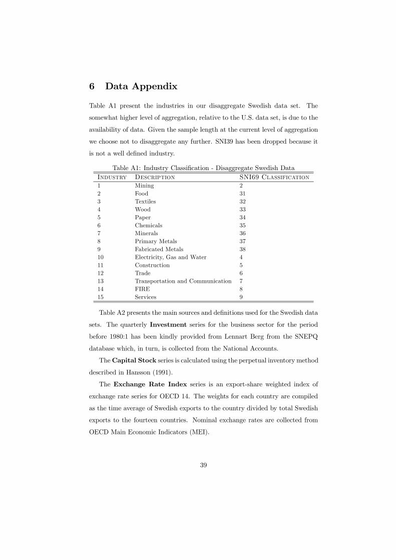
6 Data Appendix

Table A1 present the industries in our disaggregate Swedish data set. The

somewhat higher level of aggregation, relative to the U.S. data set, is due to the

availability of data. Given the sample length at the current level of aggregation

we choose not to disaggregate any further. SNI39 has been dropped because it

is not a well defined industry.

Table A1: Industry Classification - Disaggregate Swedish DataIndustry Description SNI69 Classification1 Mining 22 Food 313 Textiles 324 Wood 335 Paper 346 Chemicals 357 Minerals 368 Primary Metals 379 Fabricated Metals 3810 Electricity, Gas and Water 411 Construction 512 Trade 613 Transportation and Communication 714 FIRE 815 Services 9

Table A2 presents the main sources and definitions used for the Swedish data

sets. The quarterly Investment series for the business sector for the period

before 1980:1 has been kindly provided from Lennart Berg from the SNEPQ

database which, in turn, is collected from the National Accounts.

TheCapital Stock series is calculated using the perpetual inventory method

described in Hansson (1991).

The Exchange Rate Index series is an export-share weighted index of

exchange rate series for OECD 14. The weights for each country are compiled

as the time average of Swedish exports to the country divided by total Swedish

exports to the fourteen countries. Nominal exchange rates are collected from

OECD Main Economic Indicators (MEI).

39

The Political Dummy variable takes on the value one for years with right-

wing governments (1977-1982, 1992-1993) and zero otherwise.

Table A2: Sources and Definitions of Swedish VariablesVariable Source DefinitionY (Ac,f ,Qf ) SM Series N Gross output (A), Value added for non-farm business (Q)M (Ac,f ) SM Series N Value of used intermediary goodsH (A,Q) SM Series N Total hours worked, Total hours worked non-farm business (Q)N (A) SM Series N Number of employeesPHH (A

c) SM Series N Wage sum including collective feesV (A) SOS Industrin Consumption of electricity in gWhPV V (A

c) SOS Industrin Electricity CostI (Ac,f ,Qf ) SM Series N Investments (A), Investments for business (Q)C (Qf ) SM Series N Private consumptionP (Q) SM Series N Consumer price indexR (Q) IFS Three-month Swedish treasury bill rateM (Q) Bank of Sweden M3

.A (Q) denote annual (quarterly) series. Superscript c denotes series in current values and f denotesseries in fixed 1991 prices. SM Series N denotes the Statistics Sweden publication Statistiska Med-delanden Serie N (National Accounts). IFS denotes the IMF publication International FinancialStatistics. OECD MI denotes the OECD publication OECD Main Indicators.

The Foreign Demand Index series is an export-share weighted index of

indices for manufacturing production from MEI for OECD 14. Due to missing

data, an index of total industrial production from the OECD MEI is used as a

proxy for Germany for the period 1967-1991. For Denmark an index of industrial

production, collected from Mitchell (1992) and linked in 1970 to an index of the

production of consumer durable goods, collected from the OECD MEI, is used

as a proxy for manufacturing production.

The Real Oil Price series is compiled by converting the world spot oil price

series, obtained from IFS, to kronor using the exchange rate from the OECD

MEI and deflating using the Swedish GDP deflator from the SM Series N.

The disaggregate US data set is fully described in Jorgenson et al. (1987)

and was downloaded from Dale Jorgenson’s web site. Total hours worked and

employment was kindly provided by Jon Samuels.

40

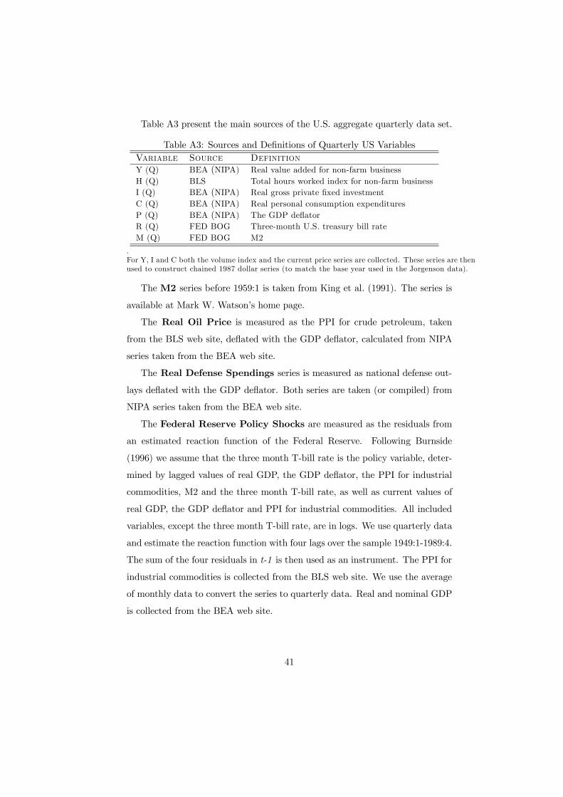
Table A3 present the main sources of the U.S. aggregate quarterly data set.

Table A3: Sources and Definitions of Quarterly US VariablesVariable Source DefinitionY (Q) BEA (NIPA) Real value added for non-farm businessH (Q) BLS Total hours worked index for non-farm businessI (Q) BEA (NIPA) Real gross private fixed investmentC (Q) BEA (NIPA) Real personal consumption expendituresP (Q) BEA (NIPA) The GDP deflatorR (Q) FED BOG Three-month U.S. treasury bill rateM (Q) FED BOG M2

.For Y, I and C both the volume index and the current price series are collected. These series are thenused to construct chained 1987 dollar series (to match the base year used in the Jorgenson data).

The M2 series before 1959:1 is taken from King et al. (1991). The series is

available at Mark W. Watson’s home page.

The Real Oil Price is measured as the PPI for crude petroleum, taken

from the BLS web site, deflated with the GDP deflator, calculated from NIPA

series taken from the BEA web site.

The Real Defense Spendings series is measured as national defense out-

lays deflated with the GDP deflator. Both series are taken (or compiled) from

NIPA series taken from the BEA web site.

The Federal Reserve Policy Shocks are measured as the residuals from

an estimated reaction function of the Federal Reserve. Following Burnside

(1996) we assume that the three month T-bill rate is the policy variable, deter-

mined by lagged values of real GDP, the GDP deflator, the PPI for industrial

commodities, M2 and the three month T-bill rate, as well as current values of

real GDP, the GDP deflator and PPI for industrial commodities. All included

variables, except the three month T-bill rate, are in logs. We use quarterly data

and estimate the reaction function with four lags over the sample 1949:1-1989:4.

The sum of the four residuals in t-1 is then used as an instrument. The PPI for

industrial commodities is collected from the BLS web site. We use the average

of monthly data to convert the series to quarterly data. Real and nominal GDP

is collected from the BEA web site.

41

Table 1: The Johansen (1991) trace test for cointegrating rankSc4 Sw Sc6 Sw K4 Sw K6 Sw Sc2 US Sc4 US K2 US K4 US

r = 0 164.58* 137.88* 124.66* 144.46*r = 1 105.21* 84.19* 77.21* 83.79* 77.49* 75.09* 74.12* 84.30*r = 2 45.35* 47.77* 47.54* 44.08* 49.26* 50.41* 45.48* 50.95*r = 3 26.80* 26.85* 26.55 22.57 29.59* 29.15* 18.21 25.24r = 4 11.66 9.91 13.14 9.83 11.43 13.96* 8.39 10.44r = 5 2.72 2.58 2.87 2.91 0.01 0.06 2.57 4.18

.* denotes significance using the 90-percent level from Osterwald-Lenum (1992).

42

Table 2: Point estimates of the cointegrating vectorsy c i m− p R π m p

Sc(4) Sw -1.061* 1.0 0.0 -0.019 0.019-1.240* 0.0 1.0 0.101 -0.101-2.152* 0.0 0.0 1.0 -1.917*

Sc(6) Sw -0.798* 1.0 0.0 0.008 -0.008-1.028 0.0 1.0 0.046 -0.046-2.992 0.0 0.0 1.0 -2.291

K(4) Sw -0.652* 1.0 0.0 0.0 -0.009 -0.001-2.907* 0.0 1.0 0.0 0.177* 0.015-0.045 0.0 0.0 1.0 -0.036* -0.017*

K(6) Sw -0.720* 1.0 0.0 0.0 -0.004 -0.004-2.909* 0.0 1.0 0.0 0.061* -0.066*0.157 0.0 0.0 1.0 -0.018 0.001

Sc(2) US -1.311* 1.0 0.0 0.104* -0.104*-1.068* 0.0 1.0 0.685* -0.685*-1.332* 0.0 0.0 1.0 -0.886*

Sc(4) US -1.261* 1.0 0.0 0.104* -0.104-0.942* 0.0 1.0 -0.340* 0.340*-2.132 0.0 0.0 1.0 -0.358*

K(2) US -0.863* 1.0 0.0 0.0 0.056* -0.073*-0.608* 0.0 1.0 0.0 0.116* 0.177*-1.193* 0.0 0.0 1.0 -0.007 0.007

K(4) US -0.704 1.0 0.0 0.0 0.025* -0.069*-0.608 0.0 1.0 0.0 0.023 -0.110*-1.193 0.0 0.0 1.0 -0.001 0.009*

.* denotes significance at the 90 percent level.

43

Table 3: Swedish Disaggregate ResultsHours correction Electricity correction

Groups ARTS γ Sargan ARTS SarganMining 1.39 1.12 (0.30) 0.36 − −

Non Durables 1.26 − 0.69 1.18 0.93Durables 1.24 − 0.39 1.17 0.50

Services and Others 1.08 − 0.43 − −NDF Correction DF Correction

Relevance Measures ∆bx ∆hpe ∆ex ∆bx ∆hpe ∆exAverage R2 0.46 0.24 0.51 0.29 0.01 0.36

Average Partial R2 0.41 0.22 0.51 0.23 -0.03 0.36

.Sample 1968-1993. The ARTS column presents the average returns to scale by group. The gammacolumn gives point estimates of the hours per employee coefficient (s.e. in parenthesis). The Sargancolumn presents the p-value of the Sargan-test of overidentfying restrictions. Average R2 and AveragePartial R2 corresponds to averages of R2 and Partial R2:s (defined as in Shea (1997)) across allindustries. DF/NDF indicates if a degrees of freedom correction is done or not, respectively.

Table 4: U.S. Disaggregate ResultsHours correction Electricity correction

Groups ARTS γ Sargan ARTS SarganMining 0.94 0.59 (0.61) 0.42 − −

Non Durables 0.69 1.69 (0.48) 0.50 0.76 0.08Durables 1.05 0.76 (0.36) 0.93 1.02 0.90

Services and Others 0.70 0.70 (0.73) 0.07 − −NDF Correction DF Correction

Relevance Measures ∆bx ∆hpe ∆ex ∆bx ∆hpe ∆exAverage R2 0.16 0.14 0.17 0.09 0.06 0.10

Average Partial R2 0.09 0.08 0.17 0.04 0.03 0.10

.Sample 1950-1989. The ARTS column presents the average returns to scale by group. The gammacolumn gives point estimates of the hours per employee coefficient (s.e. in parenthesis). The Sargancolumn presents the p-value of the Sargan-test of overidentfying restrictions. Average R2 and AveragePartial R2 corresponds to averages of R2 and Partial R2:s (defined as in Shea (1997)) across allindustries. DF/NDF indicates if a degrees of freedom correction is done or not, respectively.

44

Table 5: Correlations - Swedish Private Economy∆yA ∆xA ∆hA S BK Sc(4) K(4)

Output Growth 1Input Growth 0.78* 1Hours Growth 0.78* 0.98* 1Solow 0.71* 0.12 0.15 1BK 0.11 -0.49* -0.49* 0.73* 1Scand (4) -0.23 -0.44* -0.45* 0.12 0.36 1King (4) 0.20 -0.07 -0.05 0.41 0.25 0.71* 1Galí (4) -0.04 -0.43* -0.40 0.42* 0.50* 0.19 0.21BER -0.00 -0.65* -0.57* 0.50* 0.91* - -

.Sample 1972-1993. * denotes correlation significantly different from zero on the five-percent level.The correlations with BER are compiled on aggregates for the manufacturing sector.

Table 6: Correlations - U.S. Private Economy∆yA ∆xA ∆hA S BK Sc(2) K(2)R

Output Growth 1Input Growth 0.66* 1Hours Growth 0.77* 0.94* 1Solow 0.81* 0.09 0.29 1BK 0.16 -0.49* -0.34* 0.59* 1Scand (2) 0.18 -0.29 -0.28 0.47* 0.46* 1King (2) R 0.17 -0.25 -0.23 0.42* 0.31 0.72* 1Galí (3) 0.01 -0.30 -0.35* 0.24 0.43* 0.63* 0.40*BER 0.20 -0.43* -0.34* 0.59* 0.76* - -

.Sample 1955-1989. * denotes correlation significantly different from zero on the five-percent level.The correlations with BER are compiled on aggregates for the manufacturing sector. The R markerdenotes models with restrictions imposed the cointegrating vectors

45

Table 7: Robustness of Correlations - Swedish Private Economy∆yA ∆hA S BK K4 K6 Sc4 Sc6 Sc4R Sc6R G4

K(4) 0.19 -0.03 0.40 0.24 1K(6) 0.32 0.19 0.34 0.04 0.91* 1Sc(4) -0.24 -0.46* 0.12 0.37 0.71* 0.55* 1Sc(6) 0.02 -0.07 0.13 0.09 0.68* 0.73* 0.73* 1Sc(4)R 0.13 0.04 0.19 0.05 0.60* 0.42 0.62* 0.62* 1Sc(6)R 0.29 0.34 0.15 -0.16 0.03 0.15 -0.11 0.50* 0.41 1G(4) -0.08 -0.36 0.34 0.42 0.19 -0.10 0.19 -0.08 0.34 -0.05 1G(5) -0.06 -0.30 0.29 0.35 0.02 -0.20 0.10 -0.10 0.22 0.02 0.93*

.Sample 1973-1993. K denotes the King model , Sc is the Scandinavian model and G is the Galímodel. Number of lags in paranthesis. The R marker denotes models with restrictions imposed onthe cointegrating vectors. * denotes correlation significantly different from zero on the five-percentlevel.

Table 8: Robustness of Correlations - US Private Economy∆yA ∆hA S BK K2 K4 K2R K4R Sc2 Sc4 G3

K(2) 0.39* -0.06 0.60* 0.31 1K(4) 0.43* 0.12 0.50* 0.15 0.88* 1K(2)R 0.23 -0.21 0.50* 0.31 0.88* 0.64* 1K(4)R 0.19 -0.19 0.43* 0.22 0.82* 0.70* 0.92* 1Sc(2) 0.20 -0.28 0.50* 0.46* 0.68* 0.51* 0.73* 0.58* 1Sc(4) 0.26 -0.24 0.57* 0.46* 0.77* 0.58* 0.87* 0.76* 0.90* 1G(3) 0.04 -0.34* 0.29 0.42* 0.40* 0.31 0.39* 0.33 0.63* 0.55* 1G(4) 0.05 -0.33 0.32 0.41* 0.42* 0.33 0.39* 0.35* 0.64* 0.55* 0.98*

.Sample 1956-1989. K denotes the King model , Sc is the Scandinavian model and G is the Galímodel. Number of lags in paranthesis. The R marker denotes models with restrictions imposed onthe cointegrating vectors. * denotes correlation significantly different from zero on the five-percentlevel.

46

Table 9: The Share of the Three-Year FEVD of Aggregate Output Growth Due

to Technology Shocks.∆yA, Sweden ∆yA, U. S.

King (4/2) 15.4 15.3King (6/4) 14.7 14.4King (2) R 16.0King (4) R 23.4Scand (4/2) 10.4 13.1Scand (6/4) 7.4 12.3Scand (4) R 10.9Scand (6) R 11.8

The R marker denotes models with restrictions imposed the cointegrating vectors.

Table 10: Average Correlations Across Industries - Swedish DataBK BER G(1)

BK 1

BER 0.93 1(8/0)

Galí (1) 0.27 0.16 1(4/0) (0/0)

Galí (4) 0.30 0.21 0.64(5/0) (1/0) (15/1)

.Sample 1968-1993. Averages over 15 Industries (8 industries for correlations with BER). Numberof significant correlations on the five-percent level / Number of significant correlations on the five-percent level with other sign than reported for the average correlation in parenthesis.

Table 11: Average Correlations Across Industries - U.S. DataBK BER G(1)

BK 1

BER 0.83 1(21/0)

Galí (1) 0.55 0.50 1(27/0) (17/0)

Galí (4) 0.45 0.40 0.78(26/0) (14/0) (33/0)

.Sample 1953-1989. Averages over 33 Industries (21 industries for correlations with BER). Numberof significant correlations on the five-percent level / Number of significant correlations on the five-percent level with other sign than reported for the average correlation in parenthesis.

47

Working Paper Series/Arbetsrapport FIEF Working Paper Series was initiated in 1985. A complete list is available from FIEF upon request. Information about the series is also available at our website on URL http://www.fief.se/Publications/WP.html. 1999 149. Vartiainen, Juhana, “Job Assignment and the Gender Wage Differential: Theory and Evidence on Finnish Metalworkers”, 24 pp. 150. Gustavsson, Patrik and Nordström, Jonas, “The Impact of Seasonal Unit Roots and Vector ARMA Modeling on Forecasting Monthly Tourism Flows”, 21 pp. 151. Zetterberg, Johnny, “Arbetslöshetstider i Sverige – utvecklingen 1976-97”, 45 s. 152. Hansson, Pär, “Relative Demand for Skills in Swedish Manufacturing: Techno-logy or Trade?”, 36 pp. 153. Lundborg, Per, “Work Morale and Economic Growth”, 25 pp. 154. Agell, Jonas and Lundborg, Per, ”Survey Evidence on Wage Rigidity: Sweden in the 1990s”, 31 pp. 155. Vartiainen, Juhana, “Relative Wages in Monetary Union and Floating”, 20 pp. 156. Persson, Joakim, “Demographic and Per Capita Income Dynamics: A Convergence Study on Demographics, Human Capital, and Per Capita Income for the US States”, 42 pp. 157. Agell, Jonas, Persson, Mats and Sacklén, Hans, “Labor Supply Prediction When Tax Avoidance Matters”, 34 pp. 2000 158. Antelius, Jesper, “Sheepskin Effects in the Returns to Education: Evidence on Swedish Data”, 17 pp. 159. Erixon, Lennart, “The ‘Third Way’ Revisited. A Revaluation of the Swedish Model in the Light of Modern Economics”, 97 pp. 160. Lundborg, Per, “Taxes, Risk Aversion and Unemployment Insurance as Causes for Wage Rigidity”, 16 pp.

161. Antelius, Jesper and Lundberg, Lars, “Competition, Market Structure and Job Turnover”, 27 pp. 162. Johansson, Sten och Sélen, Jan, ”Arbetslöshetsförsäkringen och arbetslös-heten – En reanalys av IFAUs studie”, 46 s. 163. Edin, Per-Anders, Fredriksson, Peter and Lundborg, Per, ”Trade, Earnings, and Mobility – Swedish Evidence”, 28 pp. 164. Strauss, Tove, “Economic Reforms and the Poor”, 25 pp. 165. Strauss, Tove, “Structural Reforms, Uncertainty, and Private Investment”, 31 pp. 2001 166. Hansson, Pär, “Skill Upgrading and Production Transfer within Swedish Multinationals in the 1990s”, 27 pp. 167. Arai, Mahmood and Skogman Thoursie, Peter, “Incentives and Selection in Cyclical Absenteeism”, 15 pp. 168. Hansen, Sten and Persson, Joakim, “Direkta undanträngningseffekter av arbetsmarknadspolitiska åtgärder”, 27 pp. 169. Arai, Mahmood and Vilhelmsson, Roger, ”Immigrants’ and Natives’ Unemployment-risk: Productivity Differentials or Discrimination?”, 27 pp. 170. Johansson, Sten och Selén, Jan, ”Arbetslöshetsförsäkringen och arbetslös-heten (2). Reformeffekt vid 1993 års sänkning av ersättningsgraden i arbetslöshets-försäkringen?”, 39 pp. 171. Johansson, Sten, ”Conceptualizing and Measuring Quality of Life for National Policy”, 18 pp. 172. Arai, Mahmood and Heyman, Fredrik, “Wages, Profits and Individual Unemployment Risk: Evidence from Matched Worker-Firm Data”, 27 pp. 173. Lundborg, Per and Sacklén, Hans, “Is There a Long Run Unemployment-Inflation Trade-off in Sweden?”, 29 pp. 174. Alexius, Annika and Carlsson, Mikael, “Measures of Technology and the Business Cycle: Evidence from Sweden and the U.S.”, 47 pp.