Measurements of thermophysical properties of solid and ...
13
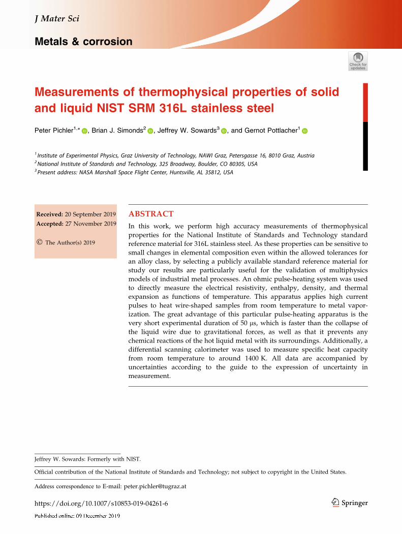
METALS & CORROSION Measurements of thermophysical properties of solid and liquid NIST SRM 316L stainless steel Peter Pichler 1, * , Brian J. Simonds 2 , Jeffrey W. Sowards 3 , and Gernot Pottlacher 1 1 Institute of Experimental Physics, Graz University of Technology, NAWI Graz, Petersgasse 16, 8010 Graz, Austria 2 National Institute of Standards and Technology, 325 Broadway, Boulder, CO 80305, USA 3 Present address: NASA Marshall Space Flight Center, Huntsville, AL 35812, USA Received: 20 September 2019 Accepted: 27 November 2019 Ó The Author(s) 2019 ABSTRACT In this work, we perform high accuracy measurements of thermophysical properties for the National Institute of Standards and Technology standard reference material for 316L stainless steel. As these properties can be sensitive to small changes in elemental composition even within the allowed tolerances for an alloy class, by selecting a publicly available standard reference material for study our results are particularly useful for the validation of multiphysics models of industrial metal processes. An ohmic pulse-heating system was used to directly measure the electrical resistivity, enthalpy, density, and thermal expansion as functions of temperature. This apparatus applies high current pulses to heat wire-shaped samples from room temperature to metal vapor- ization. The great advantage of this particular pulse-heating apparatus is the very short experimental duration of 50 ls, which is faster than the collapse of the liquid wire due to gravitational forces, as well as that it prevents any chemical reactions of the hot liquid metal with its surroundings. Additionally, a differential scanning calorimeter was used to measure specific heat capacity from room temperature to around 1400 K. All data are accompanied by uncertainties according to the guide to the expression of uncertainty in measurement. Jeffrey W. Sowards: Formerly with NIST. Official contribution of the National Institute of Standards and Technology; not subject to copyright in the United States. Address correspondence to E-mail: [email protected] https://doi.org/10.1007/s10853-019-04261-6 J Mater Sci Metals & corrosion
Transcript of Measurements of thermophysical properties of solid and ...
METALS & CORROSION
Measurements of thermophysical properties of solid
and liquid NIST SRM 316L stainless steel
Peter Pichler1,* , Brian J. Simonds2 , Jeffrey W. Sowards3 , and Gernot Pottlacher1
1 Institute of Experimental Physics, Graz University of Technology, NAWI Graz, Petersgasse 16, 8010 Graz, Austria2National Institute of Standards and Technology, 325 Broadway, Boulder, CO 80305, USA3Present address: NASA Marshall Space Flight Center, Huntsville, AL 35812, USA
Received: 20 September 2019
Accepted: 27 November 2019
� The Author(s) 2019
ABSTRACT
In this work, we perform high accuracy measurements of thermophysical
properties for the National Institute of Standards and Technology standard
reference material for 316L stainless steel. As these properties can be sensitive to
small changes in elemental composition even within the allowed tolerances for
an alloy class, by selecting a publicly available standard reference material for
study our results are particularly useful for the validation of multiphysics
models of industrial metal processes. An ohmic pulse-heating system was used
to directly measure the electrical resistivity, enthalpy, density, and thermal
expansion as functions of temperature. This apparatus applies high current
pulses to heat wire-shaped samples from room temperature to metal vapor-
ization. The great advantage of this particular pulse-heating apparatus is the
very short experimental duration of 50 ls, which is faster than the collapse of
the liquid wire due to gravitational forces, as well as that it prevents any
chemical reactions of the hot liquid metal with its surroundings. Additionally, a
differential scanning calorimeter was used to measure specific heat capacity
from room temperature to around 1400 K. All data are accompanied by
uncertainties according to the guide to the expression of uncertainty in
measurement.
Jeffrey W. Sowards: Formerly with NIST.
Official contribution of the National Institute of Standards and Technology; not subject to copyright in the United States.
Address correspondence to E-mail: [email protected]
https://doi.org/10.1007/s10853-019-04261-6
J Mater Sci
Metals & corrosion
Introduction
The National Institute of Standards and Technology
(NIST) standard reference material (SRM) for 316L
stainless steel (1155a) has recently been used for
studies of intense laser light coupling in metal to
provide data for the validation of multiphysics
models of industrial laser processes like welding,
cutting, and additive manufacturing [1]. In order to
reduce the costs associated with empirical trial-and-
error production development, manufacturers are
increasingly looking to multiphysics computer sim-
ulations to more rapidly optimize process parame-
ters. Generally, these models simulate the laser
heating of metal followed by heat flow and fluid
transport of the solid/molten metal system in order
to predict the evolution of the fusion zone and sur-
rounding heat-affected zone. Therefore, in addition to
laser light coupling they also require many thermo-
physical material properties over a very wide tem-
perature range across solid and liquid phases.
Ideally, modelers would be able to find accurate
thermophysical property values with known uncer-
tainties spanning the wide temperature range neces-
sary for the exact alloy composition they are
modeling. However, due to the limited amount of
data available modelers often resort to using values
for materials of similar, but not exact, composition to
that which they are studying, and extrapolate for
values at temperatures not found in the literature.
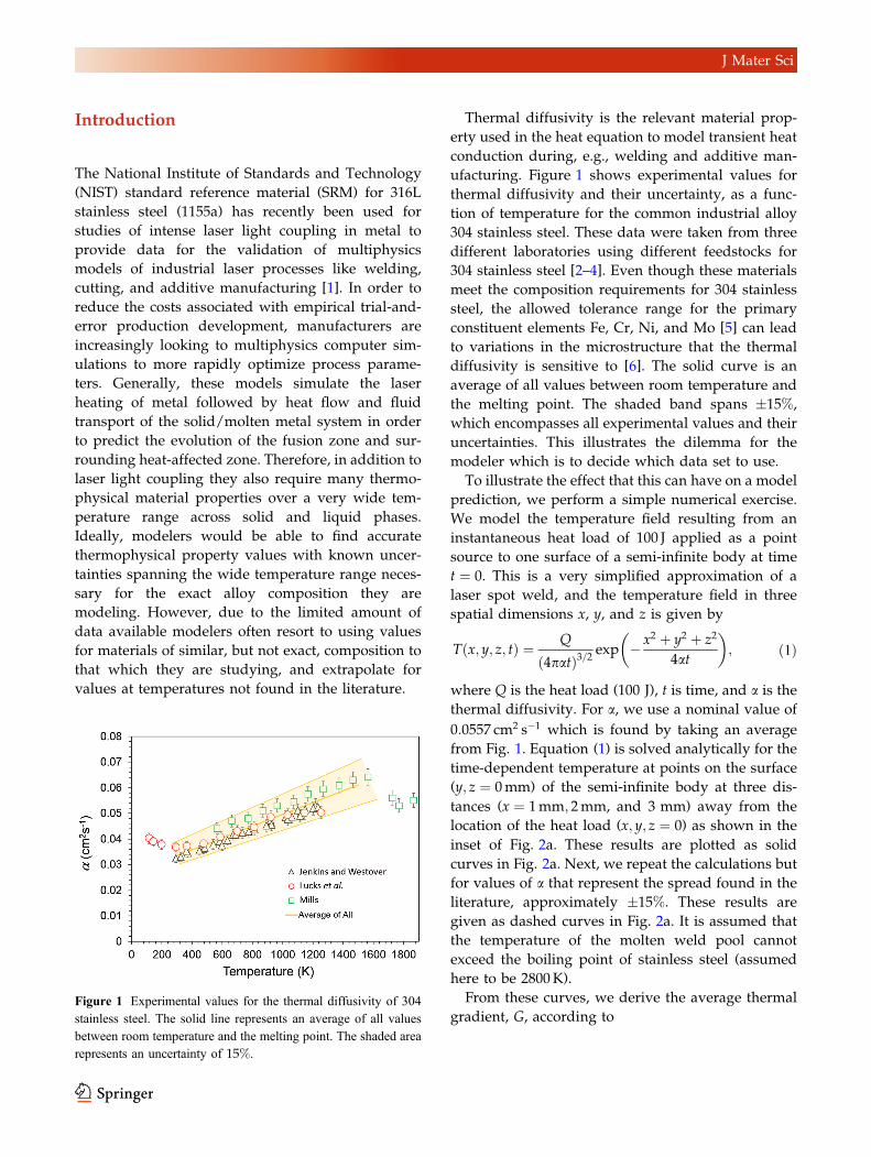
Thermal diffusivity is the relevant material prop-
erty used in the heat equation to model transient heat
conduction during, e.g., welding and additive man-
ufacturing. Figure 1 shows experimental values for
thermal diffusivity and their uncertainty, as a func-
tion of temperature for the common industrial alloy
304 stainless steel. These data were taken from three
different laboratories using different feedstocks for
304 stainless steel [2–4]. Even though these materials
meet the composition requirements for 304 stainless
steel, the allowed tolerance range for the primary
constituent elements Fe, Cr, Ni, and Mo [5] can lead
to variations in the microstructure that the thermal
diffusivity is sensitive to [6]. The solid curve is an
average of all values between room temperature and
the melting point. The shaded band spans �15%,
which encompasses all experimental values and their
uncertainties. This illustrates the dilemma for the
modeler which is to decide which data set to use.
To illustrate the effect that this can have on a model
prediction, we perform a simple numerical exercise.
We model the temperature field resulting from an
instantaneous heat load of 100 J applied as a point
source to one surface of a semi-infinite body at time
t ¼ 0. This is a very simplified approximation of a
laser spot weld, and the temperature field in three
spatial dimensions x, y, and z is given by
Tðx; y; z; tÞ ¼ Q
4patð Þ3=2exp � x2 þ y2 þ z2
4at
� �; ð1Þ
where Q is the heat load (100 J), t is time, and a is the
thermal diffusivity. For a, we use a nominal value of
0:0557 cm2 s�1 which is found by taking an average
from Fig. 1. Equation (1) is solved analytically for the
time-dependent temperature at points on the surface
(y; z ¼ 0mm) of the semi-infinite body at three dis-
tances (x ¼ 1mm; 2mm, and 3 mm) away from the
location of the heat load (x; y; z ¼ 0) as shown in the
inset of Fig. 2a. These results are plotted as solid
curves in Fig. 2a. Next, we repeat the calculations but
for values of a that represent the spread found in the
literature, approximately �15%. These results are
given as dashed curves in Fig. 2a. It is assumed that
the temperature of the molten weld pool cannot
exceed the boiling point of stainless steel (assumed
here to be 2800K).
From these curves, we derive the average thermal
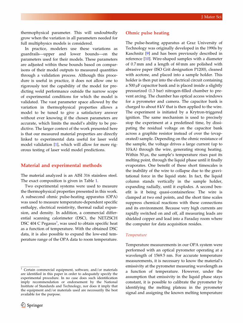
gradient, G, according toFigure 1 Experimental values for the thermal diffusivity of 304
stainless steel. The solid line represents an average of all values
between room temperature and the melting point. The shaded area
represents an uncertainty of 15%.
J Mater Sci
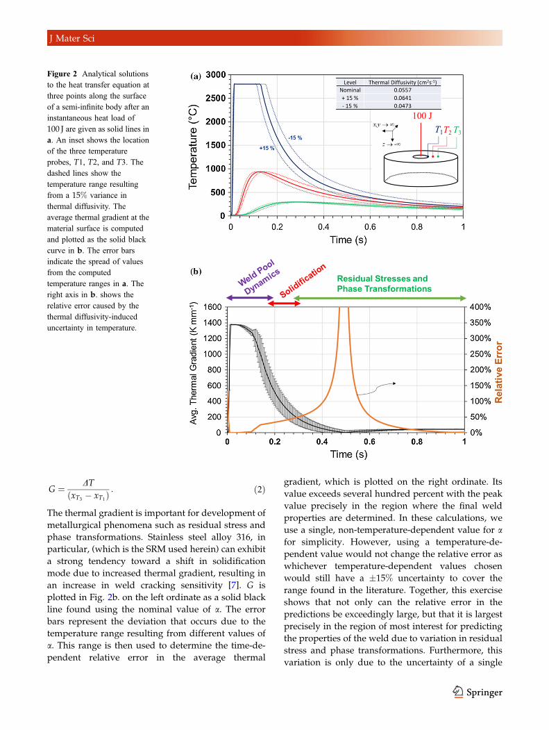
G ¼ DTxT3
� xT1ð Þ : ð2Þ
The thermal gradient is important for development of
metallurgical phenomena such as residual stress and
phase transformations. Stainless steel alloy 316, in
particular, (which is the SRM used herein) can exhibit
a strong tendency toward a shift in solidification
mode due to increased thermal gradient, resulting in
an increase in weld cracking sensitivity [7]. G is
plotted in Fig. 2b. on the left ordinate as a solid black
line found using the nominal value of a. The error
bars represent the deviation that occurs due to the
temperature range resulting from different values of
a. This range is then used to determine the time-de-
pendent relative error in the average thermal
gradient, which is plotted on the right ordinate. Its
value exceeds several hundred percent with the peak
value precisely in the region where the final weld
properties are determined. In these calculations, we
use a single, non-temperature-dependent value for afor simplicity. However, using a temperature-de-
pendent value would not change the relative error as
whichever temperature-dependent values chosen
would still have a �15% uncertainty to cover the
range found in the literature. Together, this exercise
shows that not only can the relative error in the
predictions be exceedingly large, but that it is largest
precisely in the region of most interest for predicting
the properties of the weld due to variation in residual
stress and phase transformations. Furthermore, this
variation is only due to the uncertainty of a single
Figure 2 Analytical solutions
to the heat transfer equation at
three points along the surface
of a semi-infinite body after an
instantaneous heat load of
100 J are given as solid lines in
a. An inset shows the location
of the three temperature
probes, T1, T2, and T3. The
dashed lines show the
temperature range resulting
from a 15% variance in
thermal diffusivity. The
average thermal gradient at the
material surface is computed
and plotted as the solid black
curve in b. The error bars
indicate the spread of values
from the computed
temperature ranges in a. The
right axis in b. shows the
relative error caused by the
thermal diffusivity-induced
uncertainty in temperature.
J Mater Sci
thermophysical parameter. This will undoubtedly
grow when the variation in all parameters needed for
full multiphysics models is considered.
In practice, modelers use these variations as
guardrails—upper and lower bounds—on the
parameters used for their models. These parameters
are adjusted within these bounds based on compar-
isons of their model outputs to measured quantities
through a validation process. Although this proce-
dure is useful in practice, it does not allow one to
rigorously test the capability of the model for pre-
dicting weld performance outside the narrow scope
of experimental conditions for which the model is
validated. The vast parameter space allowed by the
variation in thermophysical properties allows a
model to be tuned to give a satisfactory answer
without ever knowing if the chosen parameters are
accurate, which limits the model’s ability to be pre-
dictive. The larger context of the work presented here
is that our measured material properties are directly
linked to experimental data useful for laser weld
model validation [1], which will allow for more rig-
orous testing of laser weld model predictions.
Material and experimental methods
The material analyzed is an AISI 316 stainless steel.
The exact composition is given in Table 1.
Two experimental systems were used to measure
the thermophysical properties presented in this work.
A subsecond ohmic pulse-heating apparatus (OPA)
was used to measure temperature-dependent specific
enthalpy, electrical resistivity, thermal radial expan-
sion, and density. In addition, a commercial differ-
ential scanning calorimeter (DSC), the NETZSCH
DSC 404 C Pegasus1, was used to obtain specific heat
as a function of temperature. With the obtained DSC
data, it is also possible to expand the low-end tem-
perature range of the OPA data to room temperature.
Ohmic pulse heating
The pulse-heating apparatus at Graz University of
Technology was originally developed in the 1990s by
Kaschnitz [9] and has been previously described in
reference [10]. Wire-shaped samples with a diameter
of 0:7mm and a length of 60mm are polished with
abrasive paper (ISO Grit designation P1200), cleaned
with acetone, and placed into a sample holder. This
holder is then put into the electrical circuit containing
a 500 lF capacitor bank and is placed inside a slightly
pressurized (1.3 bar) nitrogen-filled chamber to pre-
vent arcing. The chamber has optical access windows
for a pyrometer and camera. The capacitor bank is
charged to about 8 kV that is then applied to the wire.
The experiment is initiated by a Krytron-triggered
ignition. The same mechanism is used to precisely
stop the experiment at a predefined time, by dissi-
pating the residual voltage on the capacitor bank
across a graphite resistor instead of over the (evap-
orated) sample. Depending on the ohmic resistance of
the sample, the voltage drives a large current (up to
10 kA) through the wire, generating strong heating.
Within 50 ls, the sample’s temperature rises past its
melting point, through the liquid phase until it finally
evaporates. One benefit of these short timescales is
the inability of the wire to collapse due to the gravi-
tational force in the liquid state. In fact, the liquid
column stands vertically in the sample holder,
expanding radially, until it explodes. A second ben-
efit is it being quasi-containerless: The wire is
clamped at two end points, and the short time scales
suppress chemical reactions with these connections
and its environment. Because very high currents are
rapidly switched on and off, all measuring leads are
shielded copper and lead into a Faraday room where
the computer for data acquisition resides.
Temperature
Temperature measurements in our OPA system were
performed with an optical pyrometer operating at a
wavelength of 1569.5 nm. For accurate temperature
measurements, it is necessary to know the material’s
emissivity at the pyrometer measuring wavelength as
a function of temperature. However, under the
assumption that emissivity in the liquid phase stays
constant, it is possible to calibrate the pyrometer by
identifying the melting plateau in the pyrometer
signal and assigning the known melting temperature
1 Certain commercial equipment, software, and/or materialsare identified in this paper in order to adequately specify theexperimental procedure. In no case does such identificationimply recommendation or endorsement by the NationalInstitute of Standards and Technology, nor does it imply thatthe equipment and/or materials used are necessarily the bestavailable for the purpose.
J Mater Sci
to this value. Due to the sensitivity of the pyrometer
photodiode (InGaAs), it is not possible to measure
surface radiance below a sample temperature of
1100K. Instead, we extend the range to lower tem-
peratures by correlation with DSC results as will be
explained later.
Enthalpy
Because of the short duration of the experiment, heat
losses are negligible, and it is assumed that the elec-
trical energy is completely converted into heat. Thus,
it is possible to determine the supplied specific heat
QSðtÞ by integrating the electrical power according to
QSðtÞ ¼1
m�Z t
0
Uðt0Þ � Iðt0Þ dt0; ð3Þ
where m is the mass of the specimen, Uðt0Þ the volt-
age drop along the specimen at time t0, and Iðt0Þ thecurrent across the specimen at time t0. As pulse
heating is an isobaric process, the specific enthalpy is
given by Eq. (3). The voltage is measured by con-
tacting the sample with two molybdenum knives,
with a distance l between one other, and measuring
two voltage drops to a common ground. The differ-
ence of these voltage drops yields the voltage drop
Uðt0Þ along the specimen. Current is measured
inductively with a Pearson probe [11]. The mass is
determined from the diameter d of the sample at
room temperature measured with a laser micrometer,
the distance between the voltage knives l, and the
density at room temperature.
Electrical resistivity
The resistivity of a conducting material is defined as
qðtÞ ¼ RðtÞ � AðtÞlðtÞ ; ð4Þ
with R(t) the time-dependent resistance, A(t) the
time-dependent specimen cross-sectional area, and
l(t) the time-dependent length of the sample. Note
that because of the high heating rates, the length of
the sample remains unaffected during the experi-
ment, lðtÞ ¼ lðt0Þ ¼ l. According to Ohm’s law, Eq. (4)
further yields
qðtÞ ¼ UðtÞIðtÞ � dðtÞ
2 � p4 � l : ð5Þ
It is useful to define the resistivity according to the
samples initial geometry (IG) by
qIGðtÞ ¼UðtÞIðtÞ � d
2RT � p4 � lRT
; ð6Þ
with dRT and lRT the diameter and distance between
the voltage knives at room temperature (RT),
respectively. Thus, resistivity including considera-
tions of thermal expansion can be defined as
qðtÞ ¼ qIGðtÞ �dðtÞdRT
� �2
: ð7Þ
Thermal expansion and density
Thermal expansion was measured by obtaining sha-
dow images of the expanding wire every 2:5 ls. Toobtain the fast data processing rates for these exper-
iments, a mechanically masked CCD chip was used.
Only 8 pixel-rows (with 384 pixels each) of the chip
were exposed, leaving the remainder of the chip as a
fast buffer storage. Therefore, it was possible to
obtain up to 10 images of a small cross section of the
expanding wire during an experiment. The unheated
wire, with a diameter of 0.7 mm, occupies approxi-
mately 140 pixels per row. The spatial resolution is
approximately 0.6 pixels. Before the experiment was
started, a set of pictures of the cold wire was taken.
Summing over the lines of each obtained picture
produces an intensity profile from which the diame-
ter of the wire was determined by taking the full
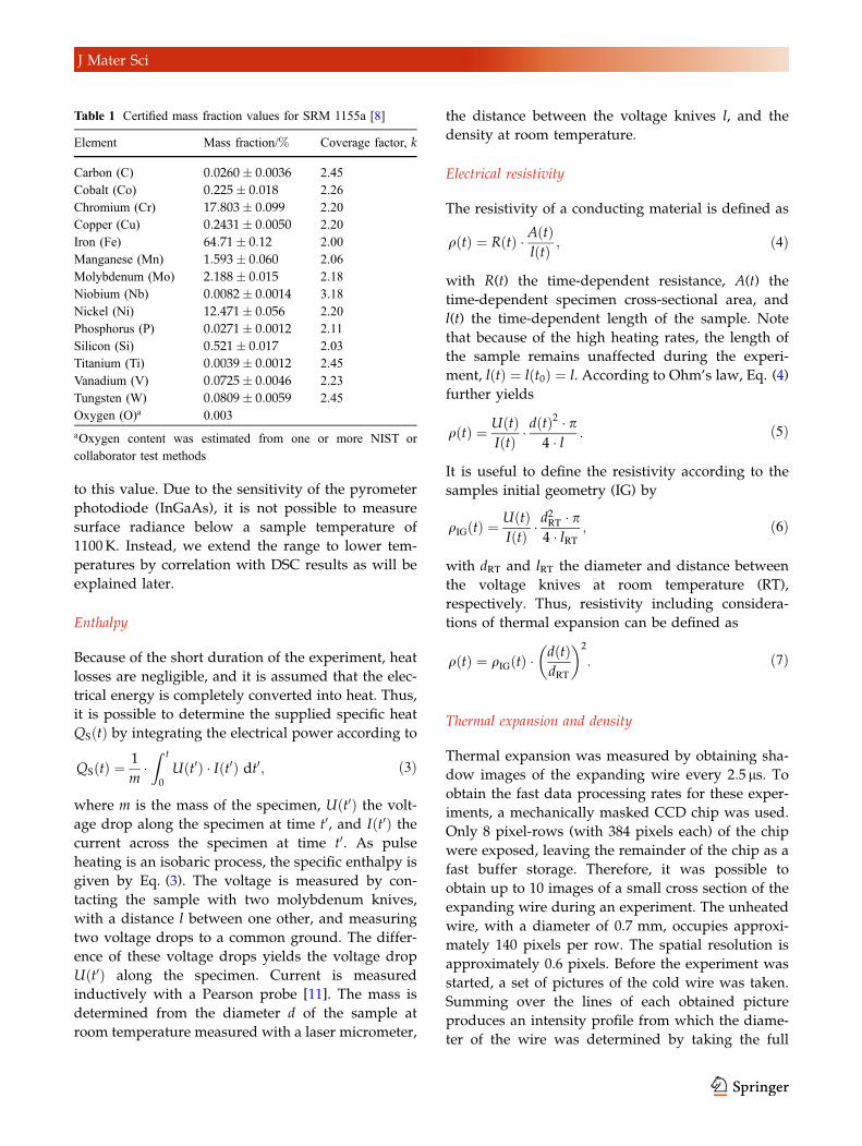
Table 1 Certified mass fraction values for SRM 1155a [8]
Element Mass fraction/% Coverage factor, k
Carbon (C) 0:0260� 0:0036 2.45
Cobalt (Co) 0:225� 0:018 2.26
Chromium (Cr) 17:803� 0:099 2.20
Copper (Cu) 0:2431� 0:0050 2.20
Iron (Fe) 64:71� 0:12 2.00
Manganese (Mn) 1:593� 0:060 2.06
Molybdenum (Mo) 2:188� 0:015 2.18
Niobium (Nb) 0:0082� 0:0014 3.18
Nickel (Ni) 12:471� 0:056 2.20
Phosphorus (P) 0:0271� 0:0012 2.11
Silicon (Si) 0:521� 0:017 2.03
Titanium (Ti) 0:0039� 0:0012 2.45
Vanadium (V) 0:0725� 0:0046 2.23
Tungsten (W) 0:0809� 0:0059 2.45
Oxygen (O)a 0.003
aOxygen content was estimated from one or more NIST or
collaborator test methods
J Mater Sci
width at half maximum (FWHM) of the intensity
profile. All measured quantities shared the same time
basis due to a common trigger pulse, and a temper-
ature was assignable to each of the obtained pictures.
The volume expansion as a function of temperature
was then calculated by the ratio of the FWHM value
of the hot wire at a certain time and temperature,
d(T), to the FWHM value of the cold wire d0
VðTÞV0
¼ dðTÞd0
� �2
: ð8Þ
Equation (8) is only true when longitudinal expan-
sion of the wire is prevented and only radial expan-
sion of the wire occurs. In pulse-heating experiments,
this is the case as shown by Huepf [12].
Density as a function of temperature D(T) can then
be derived by combining the density at room tem-
perature D0 with the volume expansion
DðTÞ ¼ D0 �d0
dðTÞ
� �2
ð9Þ
with a more detailed explanation found in [13].
Differential scanning calorimeter (DSC)
To measure specific heat capacity in the solid phase
and extend the temperature range of the OPA data, a
commercial DSC, the NETZSCH DSC 404 C Pegasus,
was used. The DSC measures the temperature dif-
ference between two crucibles. For one DSC experi-
ment, a total of three measurements were performed:
One with two empty crucibles to determine the
baseline, a run with one empty crucible and a refer-
ence material in the other, and finally a run with one
empty crucible and the sample material. As a result
of the specific heat capacity of the material (reference
or sample), there is a temperature gradient between
the empty crucible and the filled one, when heating
up both equally. By measuring the temperature gra-
dient for a reference material with a known specific
heat capacity, it is possible to determine the specific
heat capacity of the sample under test. Ideally, the
temperature difference between two empty crucibles
would be zero. However, due to minor imperfections
in the alignment of the measuring system and
unequal masses of the crucibles this is not exactly
true. Thus, it is necessary to measure the baseline and
subtract it from both the reference measurements, as
well as the sample measurement. The specific heat
capacity cp;S of the sample was determined by the
equation
cp;SðTÞ ¼ cp;RðTÞ �mR
mS
/S � /B
/R � /B
; ð10Þ
H(t)
ρ (t)0
T(t)
H(T)
ρ(T)
ρ(H)
ε(t)
U(t)
I(t)
J(t)
S0 S1
S3S2
c (T)p T(H) ρ(T)
st1 Step nd2 Step 4th Steprd3 Step
Base Quantities(measured)
Calculated Quantities derived from Base Quantities
Enthalpy
Uncorrected, ElectricalResistivity
Temperature
Enthalpy vs. Temperature
Corrected, ElectricalResistivity vs. Temperature
Corrected, ElectricalResistivity vs. Enthalpy
Normal, SpectralEmissivity
Voltage-Drop
Current
Surface Radiation
4 IndependentStokes-Vectors
Specific Heat Capacity Temperature vs. Enthalpy
Corrected, ElectricalResistivity vs. Temperature
Resistivity vs. TemperatureDSC + Pulse-heating
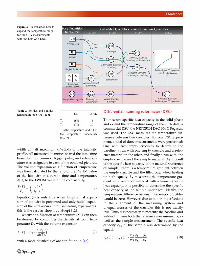
Figure 3 Flowchart on how to
expand the temperature range
for the OPA measurements
with the help of a DSC.
Table 2 Solidus and liquidus
temperature of SRM 1155a T/K DT/K
Ts 1675 15
Tl 1708 30
T is the temperature, and DT is
the temperature uncertainty
(k ¼ 2)
J Mater Sci
500
750
1000
1250
1500
1750
Tem
pera
ture
(K)
(a) DSC enthalpy dataDSC enthalpy fitsolidus temperature
200 400 600 800 1000 1200 1400
Enthalpy (kJ·kg−1)
Arb
itrar
yTem
pera
ture
(b)
pulse-heating datalinear regression
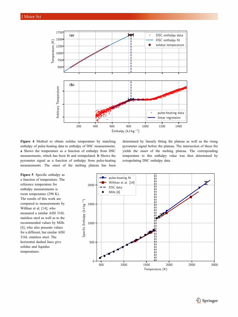
Figure 4 Method to obtain solidus temperature by matching
enthalpy of pulse-heating data to enthalpy of DSC measurements.
a Shows the temperature as a function of enthalpy from DSC
measurements, which has been fit and extrapolated. b Shows the
pyrometer signal as a function of enthalpy from pulse-heating
measurements. The onset of the melting plateau has been
determined by linearly fitting the plateau as well as the rising
pyrometer signal before the plateau. The intersection of those fits
yields the onset of the melting plateau. The corresponding
temperature to this enthalpy value was then determined by
extrapolating DSC enthalpy data.
500 1000 1500 2000 2500 3000Temperature (K)
0
500
1000
1500
2000
Spec
ific
Ent
halp
y(k
J·kg−
1 )
pulse-heating fitWilthan et al. [14]DSC dataMills [4]
Figure 5 Specific enthalpy as
a function of temperature. The
reference temperature for
enthalpy measurements is
room temperature (298 K).
The results of this work are
compared to measurements by
Wilthan et al. [14], who
measured a similar AISI 316L
stainless steel as well as to the
recommended values by Mills
[4], who also presents values
for a different, but similar AISI
316L stainless steel. The
horizontal dashed lines give
solidus and liquidus
temperatures.
J Mater Sci
with T the temperature, cp;RðTÞ the specific heat
capacity of the reference material, mR the mass of the
reference, mS the mass of the sample, and /i the DSC
signals (i ¼ R,S,B; R stands for reference, S for sam-
ple, and B for baseline).
The temperature range of the DSC measurements
starts at 473K. Enthalpy can be calculated from cp;Sby integrating heat capacity with respect to
temperature:
HðTÞ ¼Z T
473K
cp;SðT0ÞdT0 þ ð473K� 298KÞ � cp;Sð473KÞ:
ð11Þ
By obtaining enthalpy as a function of temperature,
H(T), it is then possible to determine the inverse:
Temperature as a function of enthalpy T(H). As
enthalpy data obtained by OPA measurements start
from room temperature, these data can be matched
with the enthalpy data obtained from DSC
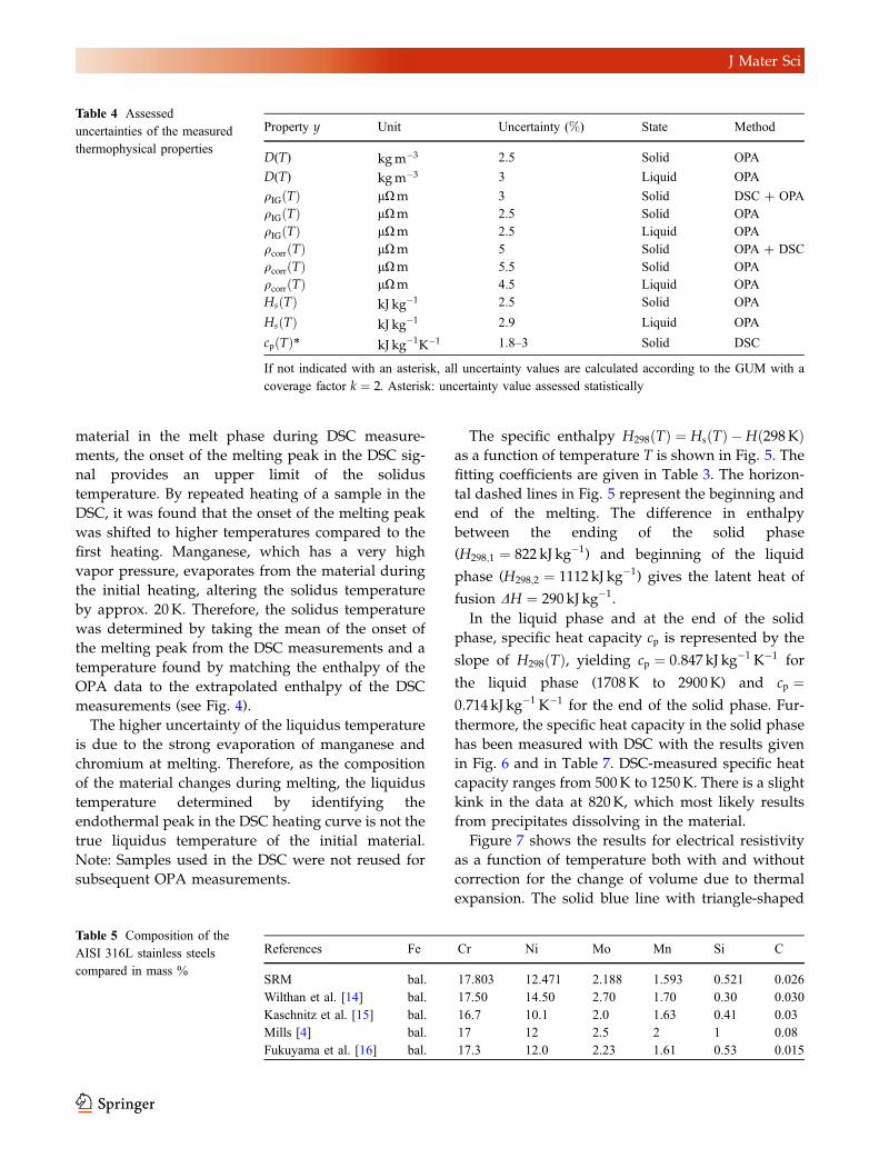
Table 3 Polynomial fit coefficients for the thermophysical properties according to y ¼ aþ bT þ cT2
Property y Unit a b c Range T/K State Method
D(T) kgm�3 8052 � 0.564 500�T�Ts s OPA
D(T) kgm�3 8065 � 0.661 Tl �T� 2900 l OPA
qIGðTÞ lXm 0.624 7:951� 10�4 �2:61� 10�7 500�T� 1250 s DSC ? OPA
qIGðTÞ lXm 1.026 1:477� 10�4 1350�T�Ts s OPA
qIGðTÞ lXm 1.263 2:021� 10�5 Tl �T� 2900 l OPA
qcorrðTÞ lXm 0.977 2:605� 10�4 1350�T�Ts s OPA
qcorrðTÞ lXm 1.154 1:893� 10�4 Tl �T� 2900 l OPA
HsðTÞ kJ kg�1 � 139 0.459 7:16� 10�5 500�T� 1250 s DSC
HsðTÞ kJ kg�1 � 374 0.714 1350�T�Ts s OPA
HsðTÞ kJ kg�1 � 335 0.847 Tl �T� 2900 l OPA
Ts ¼ 1675K, Tl ¼ 1708K, are the solidus and liquidus temperatures, respectively. D is the density, qIG is the electrical resistivity
assuming initial geometry, qcorr is the electrical resistivity corrected for thermal expansion, Hs is the specific enthalpy, and T is the
temperature. S and l denote data in solid and liquid phase
400 600 800 1000 1200Temperature (K)
0.50
0.52
0.54
0.56
0.58
0.60
0.62
0.64
Spec
ific
heat
capa
city
(kJ·k
g−1 ·K
−1)
DSC dataWilthan et al. [14]Kaschnitz et al. [15]
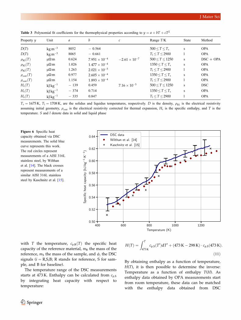
Figure 6 Specific heat
capacity obtained via DSC
measurements. The solid blue
curve represents this work.
The red circles represent
measurements of a AISI 316L
stainless steel, by Wilthan
et al. [14]. The black crosses
represent measurements of a
similar AISI 316L stainless
steel by Kaschnitz et al. [15].
J Mater Sci
measurements to assign a temperature to the
enthalpy data from OPA measurements. This is pre-
sented graphically in Fig. 3.
To determine the density at room temperature,
cylinders with a diameter of d ¼ð10:98� 0:01Þ � 10�3m and a height of h ¼ ð5:19�0:01Þ � 10�3m were machined. The mass of the
cylinder was measured with a Mettler Toledo PB303
balance as m ¼ ð3:883� 0:001Þ � 10�3kg, yielding a
room temperature density of ð7904� 25Þ kgm�3.
Results
Solidus (Ts) and liquidus (Tl) temperatures of the
material were determined by DSC measurements and
are presented in Table 2. Due to evaporation of the
500 1000 1500 2000 2500 3000Temperature (K)
1.0
1.1
1.2
1.3
1.4
1.5
1.6
1.7
1.8
Ele
ctric
alre
sist
ivity
(µΩ·m
)
combined DSC datauncor. pulse-heating fitcorr. pulse-heating fituncorr. Wilthan et al. [14]
corr. Wilthan et al. [14]Kaschnitz et al. [15]
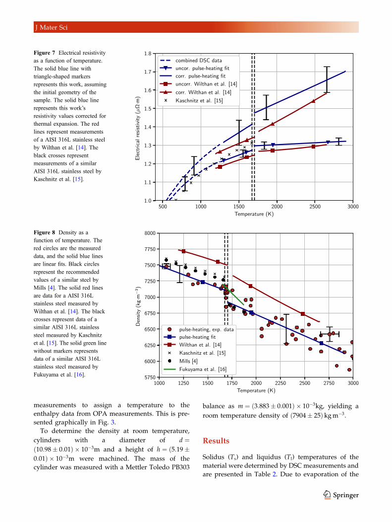
Figure 7 Electrical resistivity
as a function of temperature.
The solid blue line with
triangle-shaped markers
represents this work, assuming
the initial geometry of the
sample. The solid blue line
represents this work’s
resistivity values corrected for
thermal expansion. The red
lines represent measurements
of a AISI 316L stainless steel
by Wilthan et al. [14]. The
black crosses represent
measurements of a similar
AISI 316L stainless steel by
Kaschnitz et al. [15].
1000 1250 1500 1750 2000 2250 2500 2750 3000Temperature (K)
5750
6000
6250
6500
6750
7000
7250
7500
7750
8000
Den
sity
(kg·m
−3)
pulse-heating, exp. datapulse-heating fitWilthan et al. [14]
Kaschnitz et al. [15]
Mills [4]Fukuyama et al. [16]
Figure 8 Density as a
function of temperature. The
red circles are the measured
data, and the solid blue lines
are linear fits. Black circles
represent the recommended
values of a similar steel by
Mills [4]. The solid red lines
are data for a AISI 316L
stainless steel measured by
Wilthan et al. [14]. The black
crosses represent data of a
similar AISI 316L stainless
steel measured by Kaschnitz
et al. [15]. The solid green line
without markers represents
data of a similar AISI 316L
stainless steel measured by
Fukuyama et al. [16].
J Mater Sci
material in the melt phase during DSC measure-
ments, the onset of the melting peak in the DSC sig-
nal provides an upper limit of the solidus
temperature. By repeated heating of a sample in the
DSC, it was found that the onset of the melting peak
was shifted to higher temperatures compared to the
first heating. Manganese, which has a very high
vapor pressure, evaporates from the material during
the initial heating, altering the solidus temperature
by approx. 20K. Therefore, the solidus temperature
was determined by taking the mean of the onset of
the melting peak from the DSC measurements and a
temperature found by matching the enthalpy of the
OPA data to the extrapolated enthalpy of the DSC
measurements (see Fig. 4).
The higher uncertainty of the liquidus temperature
is due to the strong evaporation of manganese and
chromium at melting. Therefore, as the composition
of the material changes during melting, the liquidus
temperature determined by identifying the
endothermal peak in the DSC heating curve is not the
true liquidus temperature of the initial material.
Note: Samples used in the DSC were not reused for
subsequent OPA measurements.
The specific enthalpy H298ðTÞ ¼ HsðTÞ �Hð298KÞas a function of temperature T is shown in Fig. 5. The
fitting coefficients are given in Table 3. The horizon-
tal dashed lines in Fig. 5 represent the beginning and
end of the melting. The difference in enthalpy
between the ending of the solid phase
(H298;1 ¼ 822 kJ kg�1) and beginning of the liquid
phase (H298;2 ¼ 1112 kJ kg�1) gives the latent heat of
fusion DH ¼ 290 kJ kg�1.
In the liquid phase and at the end of the solid
phase, specific heat capacity cp is represented by the
slope of H298ðTÞ, yielding cp ¼ 0:847 kJ kg�1 K�1 for
the liquid phase (1708K to 2900K) and cp ¼0:714 kJ kg�1 K�1 for the end of the solid phase. Fur-
thermore, the specific heat capacity in the solid phase
has been measured with DSC with the results given
in Fig. 6 and in Table 7. DSC-measured specific heat
capacity ranges from 500K to 1250K. There is a slight
kink in the data at 820K, which most likely results
from precipitates dissolving in the material.
Figure 7 shows the results for electrical resistivity
as a function of temperature both with and without
correction for the change of volume due to thermal
expansion. The solid blue line with triangle-shaped
Table 4 Assessed
uncertainties of the measured
thermophysical properties
Property y Unit Uncertainty (%) State Method
D(T) kgm�3 2.5 Solid OPA
D(T) kgm�3 3 Liquid OPA
qIGðTÞ lXm 3 Solid DSC ? OPA
qIGðTÞ lXm 2.5 Solid OPA
qIGðTÞ lXm 2.5 Liquid OPA
qcorrðTÞ lXm 5 Solid OPA ? DSC
qcorrðTÞ lXm 5.5 Solid OPA
qcorrðTÞ lXm 4.5 Liquid OPA
HsðTÞ kJ kg�1 2.5 Solid OPA
HsðTÞ kJ kg�1 2.9 Liquid OPA
cpðTÞ* kJ kg�1K�1 1.8–3 Solid DSC
If not indicated with an asterisk, all uncertainty values are calculated according to the GUM with a
coverage factor k ¼ 2. Asterisk: uncertainty value assessed statistically
Table 5 Composition of the
AISI 316L stainless steels
compared in mass %
References Fe Cr Ni Mo Mn Si C
SRM bal. 17.803 12.471 2.188 1.593 0.521 0.026
Wilthan et al. [14] bal. 17.50 14.50 2.70 1.70 0.30 0.030
Kaschnitz et al. [15] bal. 16.7 10.1 2.0 1.63 0.41 0.03
Mills [4] bal. 17 12 2.5 2 1 0.08
Fukuyama et al. [16] bal. 17.3 12.0 2.23 1.61 0.53 0.015
J Mater Sci
markers represents the linear fits of the pulse-heating
data using the initial sample geometry. The solid blue
lines without markers are the linear fit of the pulse-
heating data corrected for volume expansion. The
dashed blue lines represent the fitted pulse-heating
data with matched temperatures from DSC mea-
surements. The uncorrected resistivity is represented
by the lower line; the corrected resistivity is repre-
sented by the upper line. The coefficients for the
polynomial fits are given in Table 3.
Density as a function of temperature is presented
in Fig. 8. The red circles are actual measurement
points with the solid blue lines the linear fits. The
coefficients and their respective temperature ranges
are given in Table 3.
Uncertainties
The uncertainties of the DSC measurements were
assessed statistically. Other uncertainties were cal-
culated according to the Guide to the Expression of
Uncertainty in Measurement (GUM) [17]. Uncertain-
ties of the fitting coefficients were calculated follow-
ing the guide by Matus [18]. Uncertainty values are
listed in Table 4.
Uncertainty values for the temperature-dependent
density were assessed by evaluating the radii of the
hot and cold wire 10 times to obtain a statistical
uncertainty. As this only accounts for uncertainty in
evaluation, the standard deviation of the obtained
radii was then doubled.
Conclusion
Thermophysical properties of NIST SRM for 316L
stainless steel (1155a), a Cr18–Ni12–Mo2 steel, were
measured by means of ohmic pulse heating in com-
bination with a differential scanning calorimeter
(DSC). These properties include specific heat capac-
ity, specific enthalpy, corrected and uncorrected
electrical resistivity, as well as density, all as a func-
tion of temperature. Our results were compared to
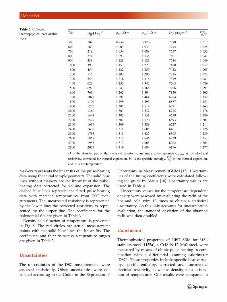
Table 6 Collected
thermophysical data of this
work
T/K HS/kJ kg�1 qIG/lXm qcorr/lXm D(T)/kgm�3 VðTÞ
V0/1
500 109 0.954 0.970 7770 1.017
600 163 1.007 1.033 7714 1.025
700 218 1.054 1.089 7657 1.033
800 274 1.093 1.138 7601 1.041
900 333 1.128 1.183 7544 1.049
1000 393 1.157 1.223 7488 1.057
1100 454 1.182 1.259 7432 1.065
1200 515 1.203 1.290 7375 1.073
1300 554 1.218 1.316 7319 1.081
1400 626 1.232 1.342 7263 1.089
1500 697 1.247 1.368 7206 1.097
1600 769 1.262 1.394 7150 1.105
1700 1042 1.291 1.464 6964 1.132
1800 1190 1.299 1.495 6857 1.151
1900 1275 1.301 1.514 6791 1.163
2000 1360 1.303 1.532 6725 1.176
2100 1444 1.305 1.551 6659 1.189
2200 1529 1.307 1.570 6593 1.201
2300 1614 1.309 1.589 6527 1.214
2400 1699 1.311 1.608 6461 1.226
2500 1783 1.313 1.627 6395 1.239
2600 1868 1.315 1.646 6329 1.251
2700 1953 1.317 1.665 6262 1.264
2800 2037 1.319 1.684 6196 1.277
D is the density, qIG is the electrical resistivity, assuming initial geometry, qcorr is the electrical
resistivity, corrected for thermal expansion, Hs is the specific enthalpy, VðTÞV0is the thermal expansion,
and T is the temperature
J Mater Sci
the literature values of similar steels, as there are no
data available in the literature for this exact SRM.
Enthalpy and uncorrected resistivity are in good
agreement to the literature. Specific heat capacity in
the liquid phase obtained in our work is 7% higher
than reported by Wilthan et al. [14] and 8.5% higher
than reported by Fukuyama et al. [16]. The value for
specific heat capacity in the liquid phase reported by
Mills [4] is 2% lower than the obtained value of this
work. Density in the liquid phase is in good agree-
ment to the values reported by Mills [4]. Our density
data are 5% lower, compared to the data reported by
Wilthan et al. [14]. The density is indirectly propor-
tional to the thermal volume expansion of the mate-
rial (see (9)). Therefore, electrical resistivity, corrected
for thermal expansion, is 5% higher, compared to the
values reported by Wilthan et al. [14]. However, it
has to be noted that the composition of the AISI 316L
steels reported in the literature differs from the
composition of the NIST SRM 1155a. The exact
compositions of the samples are shown in Table 5.
The literature data are reported as comparison values
only. Uncertainty assessment was performed
according to the GUM. Thermophysical property
data obtained in this work are listed in Tables 6 and
7. Coefficients for all fits are given in Table 3. Results
of the uncertainty assessment are listed in Table 4.
Acknowledgements
Open access funding provided by Graz University of
Technology. The authors thank Anna Vaskuri, Boris
Wilthan, and Matthias Leitner for their comments
and careful reading of this manuscript.
Compliance with ethical standards
Conflicts of interest The authors declare that there
is no conflict of interest.
Open Access This article is licensed under a Crea-
tive Commons Attribution 4.0 International License,
which permits use, sharing, adaptation, distribution
and reproduction in any medium or format, as long
as you give appropriate credit to the original
author(s) and the source, provide a link to the Crea-
tive Commons licence, and indicate if changes were
made. The images or other third party material in this
article are included in the article’s Creative Commons
licence, unless indicated otherwise in a credit line to
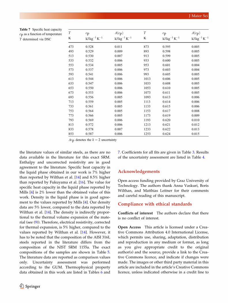
Table 7 Specific heat capacity
cp as a function of temperature
T determined via DSC
T cp DðcpÞ T cp DðcpÞK kJkg�1 K�1 kJkg�1 K�1 K kJkg�1 K�1 kJ kg�1 K�1
473 0.528 0.011 873 0.595 0.005
493 0.529 0.009 893 0.598 0.005
513 0.530 0.007 913 0.599 0.005
533 0.532 0.006 933 0.600 0.005
553 0.534 0.005 953 0.601 0.004
573 0.537 0.006 973 0.603 0.004
593 0.541 0.006 993 0.605 0.005
613 0.544 0.006 1013 0.606 0.005
633 0.547 0.006 1033 0.608 0.005
653 0.550 0.006 1053 0.610 0.005
673 0.553 0.006 1073 0.611 0.005
693 0.556 0.005 1093 0.613 0.006
713 0.559 0.005 1113 0.614 0.006
733 0.561 0.005 1133 0.615 0.006
753 0.564 0.005 1153 0.617 0.008
773 0.566 0.005 1173 0.619 0.009
793 0.569 0.006 1193 0.620 0.010
813 0.572 0.006 1213 0.621 0.012
833 0.578 0.007 1233 0.622 0.013
853 0.587 0.006 1253 0.624 0.015
Dcp denotes the k ¼ 2 uncertainty
J Mater Sci
the material. If material is not included in the article’s
Creative Commons licence and your intended use is
not permitted by statutory regulation or exceeds the
permitted use, you will need to obtain permission
directly from the copyright holder. To view a copy of
this licence, visit https://creativecommons.org/lice
nses/by/4.0/.
References
[1] Simonds BJ, Sowards J, Hadler J, Pfeif E, Wilthan B, Tanner
J, Harris C, Williams P et al (2018) Time-resolved absorp-
tance and melt pool dynamics during intense laser irradiation
of a metal. Phys Rev Appl 10(4):044061. https://doi.org/10.
1103/PhysRevApplied.10.044061
[2] Jenkins R, Westover R (1962) Thermal diffusivity of stain-
less steel from 20� to 1000� C. J Chem Eng Data
7(3):434–437. https://doi.org/10.1021/je60014a038
[3] Lucks C, Deem H (1958) Thermal properties of 13 metals:
thermal properties of 13 metals. ASTM 9:795–795. https://d
oi.org/10.1002/maco.19580091216
[4] Mills K (2002) Recommended values of thermophysical
properties for selected commercial alloys. Woodhead Pub-
lishing, Sswston
[5] Specification for Chromium and Chromium-Nickel Stainless
Steel Plate, Sheet, and Strip for Pressure Vessels and for
General Applications. https://doi.org/10.1520/a0240_a0240
m-17
[6] Mills K, Su Y, Li Z, Brooks R (2004) Equations for the
calculation of the thermo-physical properties of stainless
steel. ISIJ Int 44(10):1661–1668. https://doi.org/10.2355/isi
jinternational.44.1661
[7] Lippold L (1994) Solidification behavior and cracking sus-
ceptibility of pulsed-laser welds in austenitic stainless steels.
Weld J 73(6):129–139
[8] SRM 1155a (2013) AISI 316 Stainless Steel. National
Institute of Standards and Technology; U.S. Department of
Commerce, Gaithersburg, MD
[9] Kaschnitz E, Pottlacher G, Jaeger H (1992) A new
microsecond pulse-heating system to investigate thermo-
physical properties of solid and liquid metals. Int J Ther-
mophys 13(4):699–710. https://doi.org/10.1007/bf00501950
[10] Leitner M, Leitner T, Schmon A, Aziz K, Pottlacher G
(2017) Thermophysical properties of liquid aluminum.
Metall Mater Trans A 48:3036–3045. https://doi.org/10.100
7/s11661-017-4053-6
[11] Pearson Electronics I (2019) Pearson current monitor model
3025. http://www.pearsonelectronics.com/pdf/3025.pdf.
Accessed 05 Apr
[12] Huepf T (2010) Density determination of liquid metals:
Ph.D. thesis, Graz University of Technology
[13] Leitner M, Schroer W, Pottlacher G (2018) Density of liquid
tantalum and estimation of critical point data. Int J Ther-
mophys 39(11):124. https://doi.org/10.1007/s10765-018-24
39-3
[14] Wilthan B, Reschab H, Tanzer R, Schuetzenhoefer W, Pot-
tlacher G (2008) Thermophysical properties of a chromium–
nickel–molybdenum steel in the solid and liquid phases. Int J
Thermophys 29(1):434–444. https://doi.org/10.1007/s10765
-007-0300-1
[15] Kaschnitz E, Kaschnitz H, Schleutker T, Guelhan A Bon-
voisin B (2017) Electrical resistivity measured by millisec-
ond pulse-heating in comparison to thermal conductivity of
the stainless steel AISI 316L at elevated temperature. High
Temp High Press 46
[16] Fukuyama H, Higashi H, Yamano H (2019) Thermophysical
properties of molten stainless steel containing 5 mass% B4C.
Nucl Technol 0(0):1–10. https://doi.org/10.1080/00295450.
2019.1578572
[17] Joint Committee for Guides in Metrology (JCGM/WG 1),
WG (ed) (1993) Guide to the expression of uncertainty in
measurement: BIPM
[18] Matus M (2005) Koeffizienten und Ausgleichsrechnung: Die
Messunsicherheit nach GUM. Teil 1: Ausgleichsgeraden
(Coefficients and adjustment calculations: measurement
uncertainty under GUM. Part 1: best fit straight lines): tm—
Technisches Messen 72(10/2005). https://doi.org/10.1524/te
me.2005.72.10_2005.584
Publisher’s Note Springer Nature remains neutral with
regard to jurisdictional claims in published maps and
institutional affiliations.
J Mater Sci