Applied Scientific Research 56: 191-207, 1996.© 1996 KIIIH'erAcademic PlIhlishers. Printed in the Netherlands.

Measurements of Layer Depth during Baroclinic

Instability in a Two-Layer Flow

JOANNE M. HOLFORD and STUART B. DALZIELDepartmelll of Applied Mathematics and Theoretical Physics. Unil'ersity oj"Camhridge. SilrerStreet. Camhridge CB3 9EW, England

Received 11 September 1995; accepted in revised form 11 April 1996

191

,"

Abstract. This study investigates the baroclinic instability of a two-layer rotating fluid system. Theinstability is generated by releasing a cylinder of buoyant fluid at the surface of ambient fluid. Thebuoyant fluid is dyed so that its depth may be determined from its optical thickness. The system firstadjusts until the horizontal density gradient is balanced by a flow along the front, and the adjustedstate is then unstable to azimuthal waves. Contours of constant upper layer depth are examined,and the perturbation at each azimuthal wavenumber is determined. The initial wavenumber is wellmodelled by simple quasi-geostrophic theory. There is a clear high wavenumber cutoff, and a transferof energy to larger scales with time.

Key words: baroclinic instability, nonlinear evolution, optical thickness, Fourier descriptors

1. Introduction

A front is a region of strong horizontal gradients in fluid properties, and in generalthere is a horizontal density gradient across a front. This density structure can be

maintained in a steady state in a rotating frame if there is a velocity along thefront. The Coriolis force on moving fluid particles balances the horizontal pressure

gradient due to the density field. The system is then said to be in geostrophicbalance.

Fronts are a generic feature of ocean and atmosphere dynamics. In the ocean

they occur at many scales, from local fronts between tidally well-mixed and strat­ified waters to basin-scale fronts related to the currents of the global circulation.

Cross-front transfers of energy and momentum can be considerable, especially ifthe front is unstable, and can contribute significantly to global balances [I]. An

understanding of the dynamics of fronts is crucial to modelling the ocean system.

The flows are highly nonlinear and so expensive to model numerically. Observa­tional data from frontal regions is often hard to interpret, as the motions are relative­

ly small scale and evolve rapidly. Laboratory experiments allow the detailed study

of repeatable flows, and the investigation of a wide parameter regime. With recentlydeveloped video and image processing techniques, the flow can be observed with

good temporal and spatial resolution.

192 J.M. HOLFORD AND S.B. DALZIEL

(I)

A front can be set up on a rotating table in the laboratory by releasing a volume

of buoyant fluid at the surface of a denser fluid, both layers initially being at rest

in the rotating frame. Dyes may be added to visualise features of the flow, giving

qualitative information about the flow structure. In this paper the transparency ofdyed fluid to visible light, sometimes referred to as the optical thickness, is used

to obtain accurate quantitative measurements of the depth of the dyed upper layer.A related technique has been used to measure the average dye concentration in aplume [2]. The tank is illuminated from beneath, and the flow recorded from above

and processed using the image processing software /DJiglmage. Velocities in the

upper layer have been measured separately by the particle tracking technique [3,4], and compare well with geostrophic velocities calculated from the interface data.

The experimental apparatus and image analysis techniques are described further inSection 2.

The initial configuration is not in geostrophic balance, but the flow evolves

to a balanced state, over about two rotation periods, through a process called

Rossby adjustment. The adjusted state can be calculated theoretically, and previous

experimental data [5] agree well with the predictions. The adjustment process isdescribed in Section 3.

The upper layer cannot spread beyond the adjusted position while remaining

axisymmetric. However, as seen in previous experiments [6], !he front is ynstableto azimuthal waves, with a wavelength of approximately 21fRo, where Ro is the

deformation radius. The deformation radius is the smallest scale that is affected bythe rotation of the reference frame. For a two-layer fluid,

'2 g'Vhlh2

Ro = j2 ,

where hI and h2 are typical layer depths, g' is the reduced gravity and f is the

Coriolis parameter (twice the angular frequency of the rotating frame). As the

instabilities grow to finite amplitude, they become asymmetric and break, forminganticyclones of upper layer fluid cut off from the main patch. At the same time

cyclonic vortices form adjacent to the anticyclones, often giving an eddy pair. Waveson the scale of a local deformation radius are seen in many different situations in

the oceans, and in many cases grow to finite amplitude to produce isolated eddies.

Several classes of instability occur in stratified, rotating fluid flows. Barotropicinstability is a shear instability in a rotating frame and develops on horizontal shear

in the basic state. BarocIinic instabilities involve transfers of potential energy, andso develop in flows with a horizontal density gradient, and hence some vertical

shear. Most naturally occurring instabilities will be a mixture of ?oth kinds ofinstability, though one will often dominate. The wavelength of 21fRo seen in the

experiment reported here is typical of barocIinic instability.The simplest model of 'pure' baroclinic instability is the Phillips' model [7],

a two-layer channel flow with no horizontal shear in each layer. Results from the

equivalent linear instability in a cylindrical geometry are given in Section 4.1. Only

MEASUREMENTS OF LAYER DEPTH 193

a range of waves between a high and low wavenumber cutoff are unstable, whichis a feature of baroclinic instability resulting from a resonance of Rossby waves.

In experiments it is only possible to observe finite amplitude effects, which

may not necessarily have the same characteristics as the infinitesimal disturbances

assumed in linear stability theory. At finite amplitude the growing waves alterthe basic state, which then affects the waves themselves. Several earlier studies of

baroclinic instability have suggested that the wave that dominates at finite amplitude

is of a longer wavelength than the most unstable wave from linear theory. Suchbehaviour has been observed in the laboratory experiments of Hart [8], in which a

two-layer fluid system was driven by rotating the lid at a slightly different speed

to the rest of the container. The emergence of waves longer than the most unstablelinear mode is also predicted by weakly nonlinear theories [9, 10], applying to

slightly supercritical flows.The dominant wavenumber was determined by eye (Section 4.2), and the results

are found to be in accord with earlier studies. In the rest of Section 4, further

characteristics of the instability are explored by considering contours of constant

upper layer depth. The magnitudes of different wavenumbers are estimated by

computing the Fourier transform of a single-valued approximation of the contour

in polar coordinates, r(O). The growth rate can be estimated from the increase in(smoothed) contour length with time. The nonlinear evolution of the flow can befollowed using this method of data analysis. Conclusions are drawn in Section 5.

2. Experimental Details

2.1. CALIBRATION OF VISUALISATION SYSTEM

A Panasonic FI5 Super VHS (SVHS) video camera, with a charge couple device

(CCD) sensor, was used to record the experiments on an SVHS Panasonic AG-7330

video tape recorder (VTR). The experimental runs were then analysed by digitisingsequences of images using a Data Translation DT-2862 frame-grabber card in a 486

PC/AT computer, giving pictures with a resolution of 512 x 512 pixels and integerintensity levels 0 ::; I ::;255. Only the monochrome part of the analogue signal,

the image intensity, was recorded. Recording the colour signal as well introducedinterference and provided no additional information.

For a physical model of the absorption properties of the dye to be applicable, it is

necessary to measure a scaled absolute intensity I. The recording system of videocamera, video tape, VTR and the digitiser all distort the absolute intensity that fallson the camera lens, returning some value f(1), say. Therefore the complete system

was calibrated using a transparent grey scale which had previously been measuredby an optical densitometer. For any material subjected to incident light intensity10, resulting in transmitted intensity In, the densitometer reading an is

an = log (J~) .(2)

194

~40

220~I

~OO

t.i; >,IRO

0:;;

.§

160

2140

0120

'"~

CJ

100

~ROc; ~ 60

0Q..

40~O0

6

20 40 60

J.M. HOLFORD AND S.B. DALZIEL

80 100 120 140 160 180 200 220 ~4()

Digitised intcnsity.f(J)

Figure I. The solid line is the mapping used to relate measured intensities f(I) to absoluteintensities gn: it is a fit to the data points shown as crosses.

For these experiments, it is necessary to recover I by fitting an estimate of I-I tosome known data points U(1), 1). The calibrated scale was viewed in front of a

light source, and the digitised intensity recorded for each point on the grey scale.One distortion introduced to the system is that of automatic gain (AG): an almost

linear shift in intensities designed to give the picture a suitable overall brightness.

This was corrected by applying a linear mapping to all pixels to keep the averageintensity of two small 'reference' windows at their initial values.

In order to make the best use of the available intensity scale, digitised intensitieswere mapped onto

9n = K· IO-an')' ,

where rand K are constants. Then

(3)

(4)

a function of the absolute intensity ratio In/Im. Figure I shows 9n against I (In),with K = 275 and r = 2/3. This type of calibration has been rendered less criticalby newer cameras that exhibit a more linear response, and faster hard disk accessthat allows images to be acquired in real time.

MEASUREMENTS OF LAYER DEPTH

2.2. INVESTIGATION OF DYE TRANSPARENCY

195

Once the relationship between measured and actual intensities is known, the trans­

mission response of the dyed fluid can be examined. The dye used in all these

experiments is red Rayners food colouring. Consider light propagating in the zdirection, through a fluid layer in which the concentration varies across the layer

as c(z). Then classical absorption theory gives

dI I

clz - -l(c(z)) ,(5)

where I (c) is the scale depth associated with a concentration of dye c. It was shown,

in the plume studies [11], that the dependence of scale depth on concentration is

I (c) ex IIc. In these experiments we assume the fluid consists of two layers, alower layer with dye concentration c(z) = 0, and an upper layer with concentration

c(z) = co, a constant. An intensity In is incident on the bottom of the tank andintensity IF is the recorded foreground value. Integrating (5) gives

(6)

where cl is the upper layer depth. In practice there is a small amount of mixingbetween the two layers, leading to a more continuous dye distribution. This willnot affect the results, as the vertical integral of dye concentration is preserved, and

d then represents the effective depth of the' upper layer'.

The response of the dye used was checked by a calibration procedure, and a

typical calibration curve is shown in Figure 2. For shallow fluid layers, the behaviourfollows (6), and the scale depth l(c) is given by the slope of the curve at cl = 0, with

l(c) ex I/c. For larger depths, the transmitted intensity falls off less rapidly than

predicted, suggesting a saturation effect. As a result of this departure, the weakmixing noted above will lead to a slight over-estimate of the upper layer depth.The overall consequence of this will be minimal as mixing is largely confined to

the shallowest parts of the upper layer, where (6) holds.The depth measurements are accurate to 2% of the maximum layer depth in

shallow regions, but only to 10% in deeper regions. Larger depths can be resolved

less accurately because of the logarithmic dependence of depth on transmittedintensity. With high dye concentrations and small fluid depths, the resolution is

0.1 cm. The total volume of dye calculated from these measurements is found tobe conserved to better than 5% over 5 minutes. A correction for parallax was not

necessary as the path length of light rays varies by a factor of only 1.04 acrossthe tank. An image of the tank containing undyed fluid was averaged over 10 s toreduce noise, and used as the background image.

J.M. HOLFORD AND S.B. DALZIEL

."" .."' ..,..•.."..-~- - .

-1.0 -0.80

In(l/I/I)

-0.60 -OAO -0,20

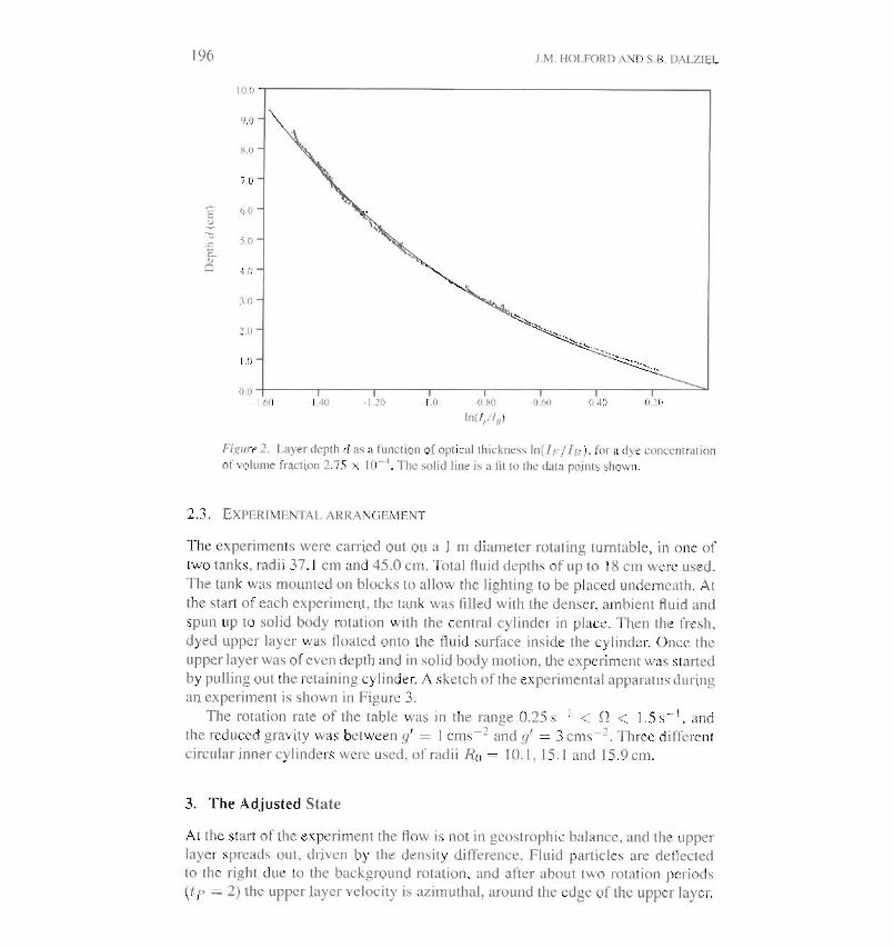
Figure 2. Layer depth If as a function of optical thickness In(I F / I B), for a dye concentrationof volume fraction 2.75 x 10-4. The solid line is a tit to the data points shown.

2.3. EXPERIMENTAL ARRANGEMENT

The experiments were carried out on a I m diameter rotating turntable, in one of

two tanks, radii 37.1 cm and 45.0 cm. Total fluid depths of up to 18 cm were used.

The tank was mounted on blocks to allow the lighting to be placed underneath. Atthe start of each experiment, the tank was filled with the denser, ambient fluid and

spun up to solid body rotation with the central cylinder in place. Then the fresh,

dyed upper layer was floated onto the fluid surface inside the cylinder. Once theupper layer was of even depth and in solid body motion, the experiment was started

by pulling out the retaining cylinder. A sketch of the experimental apparatus duringan experiment is shown in Figure 3.

The rotation rate of the table was in the range 0.25 S-l < 0 < 1.5 s-l, and

the reduced gravity was between g' = I cms-2 and g' = 3 cms-2. Three differentcircular inner cylinders were used, of radii R{) = 10.1, 15.1 and 15.9 cm.

3. The Adjusted State

At the start of the experiment the flow is not in geostrophic balance, and the upperlayer spreads out, driven by the density difference. Fluid particles are deflectedto the right due to the background rotation, and after about two rotation periods

(tp = 2) the upper layer velocity is azimuthal, around the edge of the upper layer.

MEASUREMENTS OF LAYER DEPTH 197

Figure 3. A perspective sketch of the experimental apparatus. The cylinder used to containthe buoyant fluid prior to the start of the experiment is shown, suspended above the tank. Thefour vertical bars support the video camera and related equipment.

Potential energy is released from the mean flow, and the adjusted state is one of

cyclostrophic balance, with the centrifugal component of the flow acceleration aswell as the Coriolis force balancing the horizontal pressure gradient. During the

adjustment, the interface oscillates about the adjusted position, and small-scale

shear waves grow at the edge of the upper layer. In general, these waves have

grown to finite amplitude, broken and mixed the fluid at the edge of the upper layerafter two rotation periods, but in some cases they are still visible as the baroclinicinstability develops. A greyscale image of upper layer depth during the adjustmentin which shear waves can be seen is shown in Figure 4a. Further details of the

adjustment are given in [12],

198

a

b

c

cl

e

f

J.M. HOLFORD AND S.B. DALZIEL

Figure 4. (a), (b) and (c): Greyscale images of upper layer depth at times tp = 0.9.3.3 and5.8. (d), (e) and (f); Corresponding contours at O. 30, 60 and 90% of the original upper layerdepth.

It is possible to calculate the adjusted solution analytically, without calculatingthe details of the transient motions, by using conservation principles that hold

if the flow i~hydro~tatic, The volume of the two layer~ is conserved, as i~ the

MEASUREMENTS OF LAYER DEPTH

0.0

199

-0.20

~'J-:::'-' -OAO

'-'

'-E¥:3

-0.60.~

~~-O.XO

:3 z

,oof-7.0

II

II

II

".,-,.

-6.0 -5.0 -4.0 -3.0 -2.0 -1.0 0.0 1.0 2.0

Non-dimt:nsional radial distance ti·om initial front position

Figure 5. Adjusted interface profile for one experiment. Azimuthally averaged data is takenfrom each of several images at about tp = 1.5, indicated by +. A fit to these data is shown asthe solid line, and the broken line is the theoretical adjusted solution for a circular front in a

two-layer fluid.

angular momentum of each fluid particle. This latter constraint can be rewritten todemonstrate the material conservation of shallow water potential vorticity (PY). A

graph of the adjusted interface position for one experiment is shown in Figure 5.Data is taken from several images around tp = 1.5, and the scatter in the deepest

region is in part due to the interface oscillations mentioned above. The data is fittedby

D(r) = a + btanh(r"/1.2Ro), (7)

for some a and b, and the theoretical adjusted interface position is shown for

comparison. In these experiments the initial PY distribution is modified during

adjustment, by non-hydrostatic processes. Whereas the initial PY distribution is

piecewise constant, the adjusted state has opposing PY gradients in the two layers.There is considerable potential energy stored in the adjusted state, and if theinterface were to become more horizontal, potential energy would be released.

200

4. Baroclinic Instability

J.M. HOLFORD AND S.B. DALZIEL

The adjusted state described in Section 3 develops azimuthal waves around the

edge of the upper layer, which break the axisymmetry and release potential energy.Figures 4b and c show an experiment in which six waves develop, and break to

give localised cyclonic and anticyclonic structures. The presence of opposing PVgradients in the two layers suggests that baroclinic instability through a resonance

ofRossby wave modes is a possibility, and in this section data from the experimentsis compared to a simple model of this instability.

4.1. INSTABILITY MECHANISM AND A SIMPLE MODEL

The simplest two-layer flow in a cylindrical region, radius R, that allows baroclinic

instability is solid body rotation in each layer. Azimuthal velocities are Vi = (},iT/ R,for i = 1,2, the vorticity in each layer is constant and the interface between the

layers is parabolic. There are opposing PV gradients in the two layers whenever

a, -I- 0.2, satisfying a necessary condition for baroclinic instability through aresonance of Rossby waves.

If the layers are shallow and do not vary greatly in depth, the dynamics can be

simplified to the quasi-geostrophic equations. The normal form for the perturbationstream function is

(8)

where n is the azimuthal wavenumber, and c is the angular phase speed. Thesolution is then {;i(T) = In(Nr'l R), where In is the nth Bessel function, and

N is a constant related to c and the initial perturbation amplitudes. An importantparameter is the rotational Froude number, the square of the ratio of domain

radius to the deformation radius, F = f2 R2 / g\/h, 11,2. Solving for c shows that

waves that satisfy N4 < 4# are unstable, although modes n = 0 and I are

excluded because they violate regularity at the origin. The best approximation to

the experimental flow requires that {;i (T) has only one maximum, at the edge of the

fluid region at T = R, which implies that:1: = N is the first turning point of ./n(x).

N is the equivalent, in a cylindrical geometry, to the total horizontal wavenumber

K = vk2 + [2 in a channel geometry. Only wave modes between a high and low

wavenumber cutoff are unstable. In the high wavenumber limit, N '" n + 1/2,F » I, and the wavenumber of maximum growth rate is n ~ 0.9#. In this limit,

the results asymptote to the Phillips' channel model. A

In our experiments the adjusted upper layer radius is given by R{) +pRo, where

p ~ 1.7. For a cylindrical domain of this radius, the model predicts that the mostunstable wavenumber is

n ~ 0.9(VF + p), (9)

MEASUREMENTS OF LAYER DEPTH 201

where now F = f2 R6/ g'~. Typical vertical shears in our experiments are

la, - 0,21;::::;OAJg'ho/ Ro, giving a predicted growth rate of a;::::;0.16f6'/2, where6 is the fractional depth of the upper layer.

4.2. DOMINANT WAVENUMBER

The wavenumber first observed by eye, for 2 < tp < 4, was found to be

n = 0.86( JP + 0.6) ± 1.6, (10)

in reasonable agreement with the theoretical prediction (9), and consistent with themeasurements of earlier investigators [13]. The high scatter in the result is caused

in part by the presence of the shear waves during adjustment. In some experiments

these shear waves do not dissipate before the onset of the later instability, and socan affect its scale.

A feature common to many of the experiments is the reduction of wavenumber

with time. Without any obvious pairing events, some waves grew at the expense ofothers. Similar behaviour has been observed before [13], and it was suggested that

this was due to the increasing importance of baroclinic over barotropic processes.The dominant wavenumberobserved at a later stage in each experiment, at typically

6 < tp < 8, was found to be

n = 0.71(JP + lA) ± 1.7, (11)

showing a decrease in n for all but the smallest values of F. The effective patchradius is now Ro + IARo, since the upper layer has spread by the instability

process.

4.3. AZIMUTHAL MODES FROM DEPTH CONTOUR DATA

The unstable waves were systematically analysed by studying the Fourier decom­

position of contours of constant depth of the upper layer. If the perturbed contour

radius is a single-valued function of angle 0, then it can be written as the sum ofcomplex Fourier components

00

7" = ""' f inOL "ne .n=-oo

( 12)

For small perturbations from the initially circular contours, (n ex: e(a-incr )1., where

a is the growth rate and Cr is the phase speed. At finite amplitudes, nonlinear effectswill alter the exponential growth with time, and the interface perturbation will no

longer be small compared to the interface slope of the basic state. However, the

decomposition (12) can be applied to any contour for which 7"(0) is single-valued,that is, until the waves break. Since 7" is real (12) may be written as

00

7" = L an cos (nO + <Pn),n=O

( 13)

202 J.M. HOLFORD AND S.B. DALZIEL

where the amplitude an and phase rpn are real. The nth term represents a pertur­

bation to a circle that is symmetric under rotations of 27r / 71" equivalently with 71,

axes of reflectional symmetry. Hence even after the initial infinitesimal growth, thisdecomposition still measures the relative importance of different wavenumbers.

Sequences of images were captured, and depth contours found at 0, 10, ... ,

90% of the initial depth. Examples of contours at four depths are shown at threetimes during an experiment, in Figures 4d, e and f. The distances of the curve from

the volume centre of the upper layer, at equally spaced e values, were taken as

the inputs into a fast Fourier transform (FFT) algorithm. The Fourier componentscorrespond to the coefficients (n in (12). Typically 28 points were chosen. The

wavenumber reduction seen visually occurs relatively late on in the experiments,when the waves have broken in the sense that it is no longer possible to define a

single-valued curve r( e). Therefore, when such breaking contours were processed,overlapping regions inside the contour on the downstream side, and outside the

contour on the upstream side, were excised, giving a sudden jump in r at some evalues.

4.4. RANGE OF UNSTABLE WAVENUMBERS

In all the experiments the energy was confined to a restricted band of wavenum­

bers between a high and low wavenumber cutoff, clearly present despite the high

wavenumber noise from the asymmetry of the flow. An example of perturbation

amplitudes against wavenumber is shown in Figure 6, for an instability that wasvisually wavenumber 71, = 6. The energy is confined between 2 ::; 71, ::; 7, and

reasonably evenly distributed within this range.

The upper cutoff is confirmed by an analysis of the relationship between thephases of components in contours at different depths. Figure 7 shows the wavenum­

ber phases corresponding to Figure 6. For wavenumbers 71, :S 7 the phase is gener­

ally well correlated, whereas above this cutoff it appears random.The relative importance of different wavenumbers at different depths can also

be seen in Figure 6. The same wavenumbers are prominent at all depths, but low­er wavenumbers are dominant on the deeper shorter contours. This is consistent

with the predicted Bessel function radial dependence of the instability, since lower

wavenumbers are less confined to the upper layer edge. Physically, high wavenum­bers at the centre would lead to very short scales, rather than the deformation radius

scale typical of this instability.Figure 8 shows the changing importance of the wavenumber amplitudes in

this experiment, for the 20% depth contour. For 4 < tF' < 6, the amplitudes of2 ::; 71, ::; 7 are growing whereas later 71, = 2, 3 and 5 dominate. Counting by eye,

six waves remained visible, although the distribution of waves around the edge ofthe upper layer became increasingly uneven, due to the distortion of the upper layerby the growing lower wavenumber modes.

MEASUREMENTS OF LAYER DEPTH 203

0.90

O.XO0.70'"

0.60

] 0.50} «0.40

0.300.200.100.00

0.0

2.0 4.0 6.0 X.O 10.0 12.0

Wavcnumbcr 11

14.0 16.0 IX.O 20.0

Figure 6. Perturbation amplitude an as a function of wavenumber 11 for one experiment, attp = 3.6, at a range of depths.

10%4.0"'1 ----

~OO,~

30°;.,40~'o5()iYo3.0 "'1 60%

70%SO%2.0

-&

1.0~ ~3:0.0

-1.0-2.0

-3.0

1.0 2.0 3.0 4.0 5.0 ~O 7.0 X~

Wavenumbcr 11

9.0 10.0 11.0 12.0

Figure 7. Perturbation phase CPn as a function of wavenumber 11 for the same experiment, attp = 3.6, at a range of depths.

----I

J.M. HOLFORD AND S.B. DALZIEL

/.- ..",- .....•.. -.-

204

0.340

0.3200.3000.2XO0260~~0.240

'-'0.220't

.~ 0.200c..'"

O.IXO

'tO.IW'-' or. 0.140

t:

0.120c Z 0.100

O.UXU0.0600.0400.0200.0000.0

----- 2

--- ••.. 3

.--.- 4

.- .. - .. - 5

..............6

.------ 7

----------. X---- ~10

11

p

1.0 2.0 3.0

,/

//

4.0 5.0 6.0

Time lp

/

7.0

//

H.D

,/I

9.0 100

Figure 8. Perturbation amplitude an normalised by a, the radius of the circle with the samearea as the contour, as a function of time tp for the same experiment, for the contour at 20%depth.

4.5. INCREASE IN LENGTH OF DEPTH CONTOURS

The increase in length of contours of constant depth has been studied as an indicator

of the overall increase in the magnitude of the disturbance. When the waves have

grown to finite amplitude, several disjoint contours are present for the greaterdepths, as can be seen in Figure 4f. In this case only the length of the longestcontour, encircling the central region of upper layer fluid, is considered.

Small perturbations developing at a growth rate a > 0 cause an initially circularcontour 7'(8) = an to deform to

(14 )

where c( 8) « I, and the phase speed Cr has been assumed to be negligible. It canthen be shown that

l(t) = lo + Ae2at + higher order terms, (15)

where lo = 27rao is the initial contour length. Hence it is predicted that the con­

tour length increases exponentially, with twice the growth rate of the perturbationvelocities and interface displacements.

The length of a contour from a digitised image is sensitive to the amount of

pixel-scale noise. One method of removing this noise without imposing an arbitrary

MEASUREMENTS OF LAYER DEPTH 205

2.40

2.20

~2.00

~D i!'-1.80

='

gisu"01.60u "-

is

1.40Z

1.201.00

1.0

- __ 0%

____ !O%

.• _ •. 20%

.---.30"!"

._ .. _. 40%

............ 50"!"

._._._. 60%-------- 700,'0

2.0 3.0 4.0 5.0 6.0

TimClp

7.0 8.0 10.0

Figure 9. Increase in normalised contour length, l(tp )/lo, with time tp for a range of contoursfrom the same experiment.

smoothing lengthscale is to calculate the Fourier descriptors of the curve and discardthe higher frequencies. A contour of total length I, through points (x, y) is treatedas a curve on the Argand plane, through points z = x + iy. The Fourier descriptorsare the components of the Fourier spectrum computed using .'3/1 as the independentvariable, where .'3 is the distance along the contour from the start point. Convolutedcontours, that would be multi-valued in the (r, B) representation, can be representedaccurately by this method. The contribution from the nth component drops verysharply as n increases, and typically retaining only the 60 lowest componentsproduces a smooth curve of visually identical overall shape to the original. Thelength depends only weakly on this choice of the number of components included.

4.6. GROWTH RATES

For the predicted length I (t) of a contour of given depth, there are three parametersin (15), the growth rate er, the initial amplitude of the perturbations A and the initialcontour length 10. This last parameter is chosen to be the length of a contour of thatdepth in the fitted profile of the adjusted interface depth D( r), given in (7).

The results of this analysis for a typical experiment are shown in Figure 9. Con­tours at 0, 10, ... , 70% of the initial depth are shown, for times 1.5 < t p < 10.0.All contours show an exponential increase in length, and growth rates calculatedfrom least squares fits to these curves lie in the range 0.02 < er < 0.04. Deep-

206 J.M. HOLFORD AND S.B. DALZIEL

er contours exhibit only lower wavenumber instabilities and grow more slowlythan shallower contours. At about ip = 5.0, the deepest contour shows a suddendecrease in contour length, soon followed by decreases in length of the increas­ingly shallow contours, when the upper layer fluid in the growing waves shallowssufficiently to detach from the central region at each depth. This drop is followedby an exponential increase at a similar exponent to the initial increase, showing thatthis growth rate is typical of nonlinear wave dynamics rather than the initial linearprediction. In fact, the predicted linear growth rate is (5 = 0.25, approximately 10times larger than the value measured. Growth rates estimated from particle trackingvelocity data [12] show similar low values, confirming the results from contourlength data reported here.

5. Conclusions

A technique for measuring the depth of a dyed fluid layer by calculating its opticalthickness has been presented. This method can give results of a high spatial andtemporal resolution, and is non-intrusive. The technique is applied to a study ofbaroclinic instability of an adjusted circular front.

The initial dominant wavenumber of the instability agrees well with a simpletheoretical model. The Fourier decomposition of contours of constant upper layerdepth showed that only modes between a high and low wavenumber cutoff wereunstable. The dominant wavenumber decreased slightly with time, and this transferof energy could be seen in the analysis of modes from contour data. The domi­nance of low wavenumbers in finite amplitude instabilities is thought to arise fromnonlinear interactions between the mean flow and the developing waves.

The growth rate of the instabilities was calculated from the increase in lengthof depth contours. The instability grew exponentially, but at a growth rate about10 times slower than the predicted linear growth rate. The growth rate measuredcorresponds to the fully nonlinear phase of the instability, and is probably influencedby the eddy dynamics of the evolving cyclones and anticyclones.

Acknowledgements

The authors wish to thank D.C. Cheesely, D. Lipman and B.L. Dean for technicalsupport during the laboratory work, and to S. Brown for help in preparing themanuscript. We thank Dr P.E Linden for many helpful discussions. Work reportedhere is taken from the first author's doctoral thesis [12], supported by the NaturalEnvironment Research Council.

References

1. Gill, A.E., Green, J.S.A. and Simmons, AJ., Energy partition in the large-scale ocean circulationand the production of mid-ocean eddies. Deep-Sea Res. 21 (1974) 499-528.

2. Bamett, SJ., A vertical buoyant jet with high momentum in a long ventilated tunnel..I. FluidMeek 252 (1993) 279-300.

MEASUREMENTS OF LAYER DEPTH 207

3. Dalziel, S.B., Decay of rotating turbulence: Some particle tracking experiments. Appl. 5ciemijicRes. 49 (1992) 217-244.

4. Dalziel. S.B., Rayleigh- Taylor instability: Experiments with image analysis. Dyn. Atmos. Oceans20 (1993) 127-153.

5. Saunders, P.M., The instability of a baroclinic vortex. J. Phys. Oceanogr. 3 (1973) 61-65.6. Griffiths, R.W. and Linden, P.F., The stability of vortices in a rotating stratified nuid. J. Fluid

Mech. 105 (1981) 283-316.7. Phillips, N.A., Energy transformations and meridional circulations associated with simple baro­

clinic waves in a two-level, quasi-geostrophic model. Tellus 6 (1954) 273-286.8. Hart, J.E., An experimental study of nonlinear baroclinic instability and mode selection in a large

basin. Dyn. Atmos. Oceans 4 (1980) 115-135.9. Hart, J.E., Wavenumber selection in nonlinear baroclinic instability. J. Atmos. 5ci. 38 (1981)

400-408.

10. Pedlosky, JooThe non-linear dynamics of baroclinic wave ensembles. J. Fluid Mech. 102 (1981)169-209.

11. Barnett, SJ., The dynamics of buoyant releases in confined spaces. PhD Thesis, DAMTP, Cam­bridge University (1991).

12. Holford, J.M., The evolution of a front. PhD Thesis, DAMTP, Cambridge University (1994).13. Griffiths, R.W. and Linden, P.F., Laboratory experiments on fronts. Part I: Density-driven bound­

ary currents. Geophys. Astrophys. Fluid Dyn. 19 (1982) 159-187.