Measurements of Central Tendency

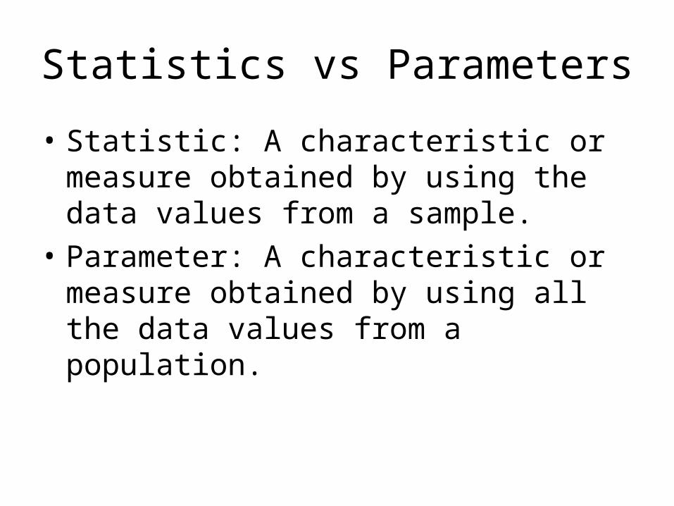
Statistics vs Parameters

• Statistic: A characteristic or measure obtained by using the data values from a sample.

• Parameter: A characteristic or measure obtained by using all the data values from a population.

Notation

• Roman Numerals: Used to denote statistics (from a sample) X

• Greek letters: Used to denote parameters (from a total population ( ) (pronounced mu)

Mean

• The sum of the values in a sample, divided by the total number of values. The symbol represents the sample mean.

• The symbol μ is used to represent the mean of a population.

X

n

x

n

xxxxX n

...321

Rounding rule for the mean

• The mean should be rounded to one more decimal place than occurs in the raw data.

• We are not always given all of the individual data when calculating the mean. Sometimes, we are given a frequency distribution and asked to calculate the mean.

Finding the mean from a frequency distribution

Class Boundaries Frequency

5.5 – 10.5 1

10.5 – 15.5 2

15.5 – 20.5 3

20.5 – 25.5 5

25.5 – 30.5 4

30.5 – 35.5 3

35.5 – 40.5 2

Find the mid point of the classClass Boundaries Frequency Midpoint

5.5 – 10.5 1 (5.5+10.5)/2 = 8

10.5 – 15.5 2 (10.5+15.5)/2=13

15.5 – 20.5 3 (15.5+20.5)/2=18

20.5 – 25.5 5 (20.5+25.5)/2=23

25.5 – 30.5 4 (25.5+30.5)/2=28

30.5 – 35.5 3 (30.5+35.5)/2 = 33

35.5 – 40.5 2 (35.5+40.5)/2=38

Multiply the frequency by the midpoint

Class Boundaries Frequency Midpoint Frequency times Midpoint

5.5 – 10.5 1 (5.5+10.5)/2 = 8 8

10.5 – 15.5 2 (10.5+15.5)/2=13 26

15.5 – 20.5 3 (15.5+20.5)/2=18 54

20.5 – 25.5 5 (20.5+25.5)/2=23 115

25.5 – 30.5 4 (25.5+30.5)/2=28 112

30.5 – 35.5 3 (30.5+35.5)/2 = 33 99

35.5 – 40.5 2 (35.5+40.5)/2=38 76

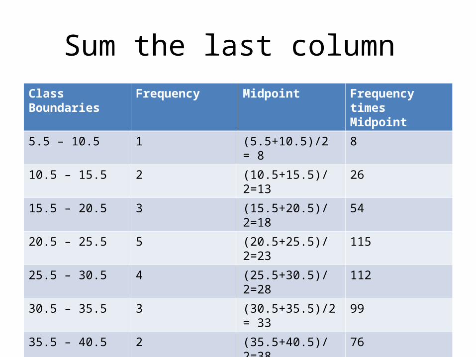
Sum the last column Class Boundaries Frequency Midpoint Frequency times

Midpoint

5.5 – 10.5 1 (5.5+10.5)/2 = 8 8

10.5 – 15.5 2 (10.5+15.5)/2=13 26

15.5 – 20.5 3 (15.5+20.5)/2=18 54

20.5 – 25.5 5 (20.5+25.5)/2=23 115

25.5 – 30.5 4 (25.5+30.5)/2=28 112

30.5 – 35.5 3 (30.5+35.5)/2 = 33 99

35.5 – 40.5 2 (35.5+40.5)/2=38 76

20 490

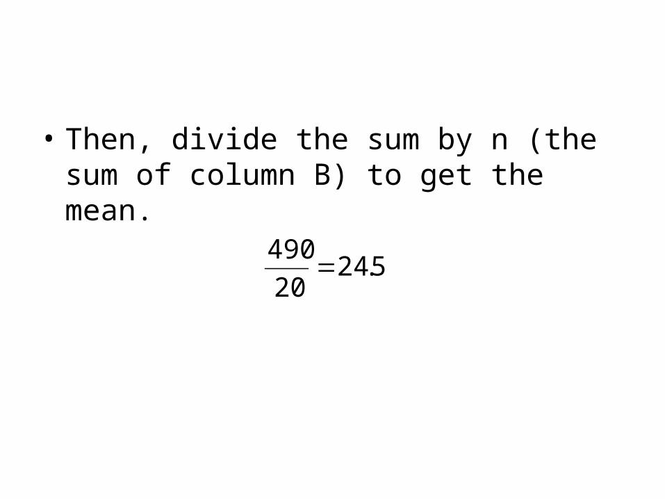
• Then, divide the sum by n (the sum of column B) to get the mean.

5.2420

490

Median

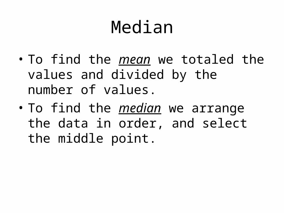
• To find the mean we totaled the values and divided by the number of values.

• To find the median we arrange the data in order, and select the middle point.

Example

• Find the median of 7, 3, 4, 5 , 9• Place in order: 3, 4, 5, 7, 9• Select the middle point

5

• If we have an even number of data in the distribution, find the middle two and add them, then divide by 2, to find the median.

• Example: Find the median of 2, 6, 5, 7, 1, 3• Place in order: 1, 2, 3, 5, 6, 7• Find the middle two points: 3, 5• Add them, divide by 2

42

53

Mode

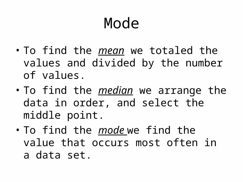
• To find the mean we totaled the values and divided by the number of values.

• To find the median we arrange the data in order, and select the middle point.

• To find the mode we find the value that occurs most often in a data set.

Example

• Find the mode of 3, 2, 4, 6, 7, 2 ,8

• Since the value 2 occurs twice, and the rest only occur once, the mode is 2

Example

• Find the mode of 3, 4, 2, 7, 8

• Each occurs only once, there is no mode

• Note that the mode is not zero, we say that there is no mode.

Example

• Find mode of 2, 3, 4, 4, 4, 5, 6, 7,7, 7, 8

• Observe that both 4 and 7 occur 3 times. • We say that the distribution is bi modal, with

modes 4 and 7

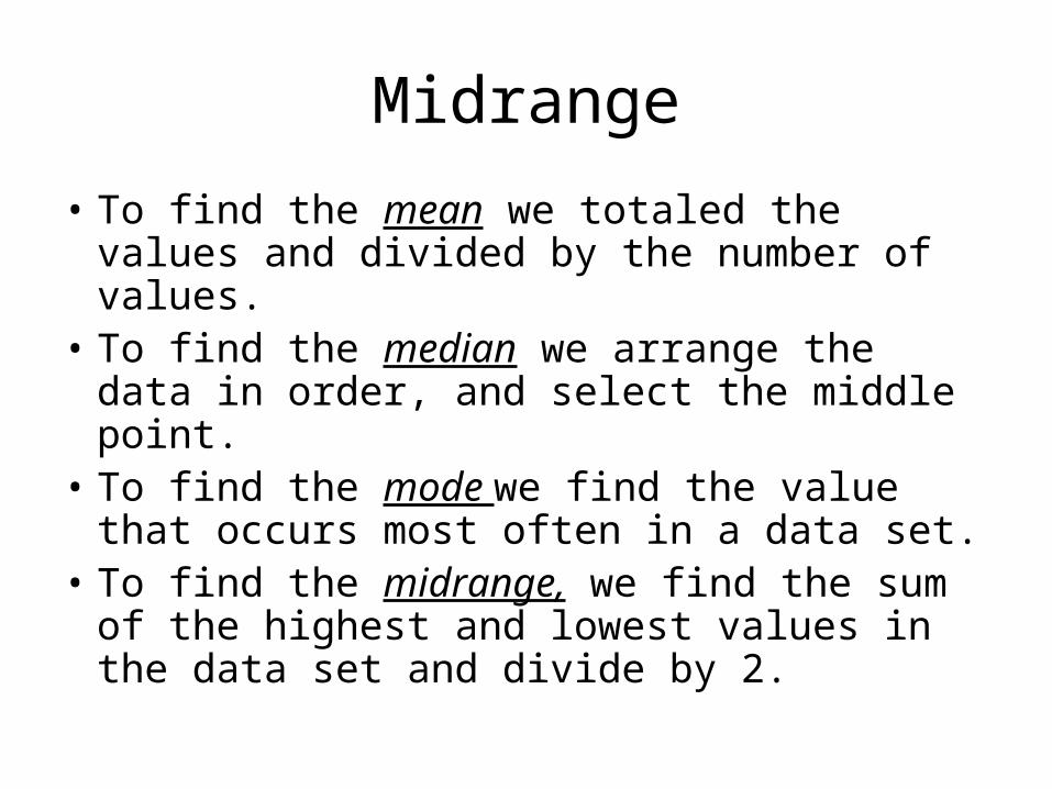
Midrange

• To find the mean we totaled the values and divided by the number of values.

• To find the median we arrange the data in order, and select the middle point.

• To find the mode we find the value that occurs most often in a data set.

• To find the midrange, we find the sum of the highest and lowest values in the data set and divide by 2.

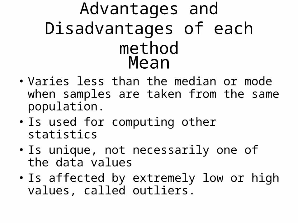
Advantages and Disadvantages of each method

Mean• Varies less than the median or mode when

samples are taken from the same population.• Is used for computing other statistics• Is unique, not necessarily one of the data

values• Is affected by extremely low or high values,

called outliers.

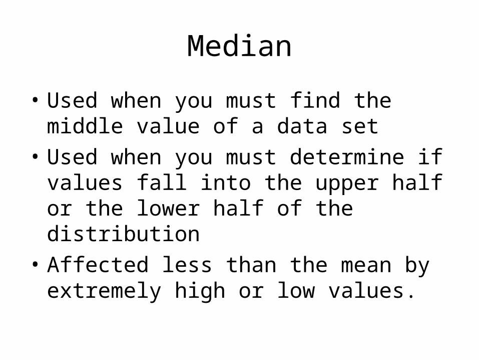
Median

• Used when you must find the middle value of a data set

• Used when you must determine if values fall into the upper half or the lower half of the distribution

• Affected less than the mean by extremely high or low values.

Mode

• Used when the most typical case is desired• Easiest to compute• Used when the data is nominal –political

preference, favorite sports team, and the like• Not always unique, may not exist

Midrange

• Easy to compute• Gives the midpoint• Affected by extremely high or low values in a

data set.

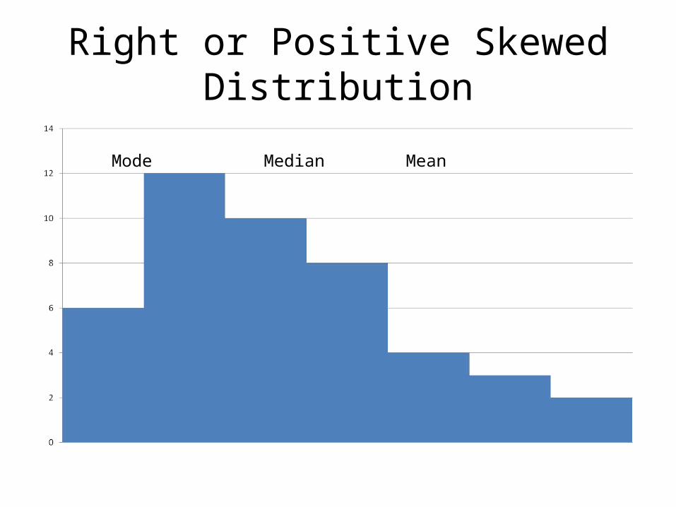
Right or Positive Skewed Distribution

Mode Median Mean

Symmetric

Left or Negative Skew