MEASUREMENT OF URANIUM AND THORIUM ABUNDANCES IN...
218
MEASUREMENT OF NEUTRINO OSCILLATION PARAMETERS AND INVESTIGATION OF URANIUM AND THORIUM ABUNDANCES IN THE EARTH USING ANTI-NEUTRINOS A DISSERTATION SUBMITTED TO THE DEPARTMENT OF PHYSICS AND THE COMMITTEE ON GRADUATE STUDIES OF STANFORD UNIVERSITY IN PARTIAL FULFILLMENT OF THE REQUIREMENTS FOR THE DEGREE OF DOCTOR OF PHILOSOPHY Kazumi Tolich March 2008
-
Upload
truongkhuong -
Category
Documents
-
view
219 -
download
2
Transcript of MEASUREMENT OF URANIUM AND THORIUM ABUNDANCES IN...
MEASUREMENT OF
NEUTRINO OSCILLATION PARAMETERS
AND
INVESTIGATION OF
URANIUM AND THORIUM ABUNDANCES IN THE EARTH
USING ANTI-NEUTRINOS
A DISSERTATION
SUBMITTED TO THE DEPARTMENT OF PHYSICS
AND THE COMMITTEE ON GRADUATE STUDIES
OF STANFORD UNIVERSITY
IN PARTIAL FULFILLMENT OF THE REQUIREMENTS
FOR THE DEGREE OF
DOCTOR OF PHILOSOPHY
Kazumi Tolich
March 2008

UMI Number: 3302880
INFORMATION TO USERS
The quality of this reproduction is dependent upon the quality of the copy
submitted. Broken or indistinct print, colored or poor quality illustrations and
photographs, print bleed-through, substandard margins, and improper
alignment can adversely affect reproduction.
In the unlikely event that the author did not send a complete manuscript
and there are missing pages, these will be noted. Also, if unauthorized
copyright material had to be removed, a note will indicate the deletion.
®
UMI UMI Microform 3302880
Copyright 2008 by ProQuest LLC.
All rights reserved. This microform edition is protected against
unauthorized copying under Title 17, United States Code.
ProQuest LLC 789 E. Eisenhower Parkway
PO Box 1346 Ann Arbor, Ml 48106-1346

© Copyright by Kazumi Tolich 2008
All Rights Reserved

I certify that I have read this dissertation and that, in my opinion, it
is fully adequate in scope and quality as a dissertation for the degree
of Doctor of Philosophy.
(Giorgio Grattaj Principal Adviser
I certify that I have read this dissertation and that, in my opinion, it
is fully adequate in scope and quality as a dissertation for the degree
of Doctor of Philosophy.
\ M ^ Y^JLJU (Martin Breidenbach)
I certify that I have read this dissertation and that, in my opinion, it
is fully adequate in scope and quality as a dissertation for the degree
of Doctor of Philosophy.
(Tsuneyoshi Kamae)
Approved for the University Committee on Graduate Studies.
iii

iv

Abstract
The Kamioka Liquid scintillator Anti-Neutrino Detector (KamLAND) was designed
to detect electron anti-neutrinos from commercial nuclear reactors, z eactorS, and the
Earth, z?geos, via inverse /?-decay. The analysis presented in this thesis measures
the mass-squared difference, A m ^ , and the mixing angle, #12, involved in neutrino
oscillation, using Reactors while simultaneously measuring the Pgeo flux. Ara^ and
812 are two of the fundamental constants of nature, whose values are not currently
predicted by the Standard Model of particle physics. The study of the Earth's interior
by measuring the ugeo flux is a new avenue in geophysics, opened by KamLAND.
This analysis significantly increases the sensitivity to neutrino oscillation parameters
compared to previous KamLAND results. The improvement is achieved by an almost
three-fold increase of statistics, the lowering of the analysis energy range as far as
allowed by the inverse /3-decay threshold, a better overall control of systematics, and
the simultaneous analysis of PreactorS and ^geos.
The null hypothesis of an undistorted Preactor energy spectrum expected in the
absence of neutrino oscillation is definitively rejected at the 99.98 % confidence level.
Instead, the measured energy distribution is consistent with the expectation from
two-flavor neutrino oscillation with sin2 29u = 0.935+O;Q65 and A m ^ = 7.44lo;}g x
10~5eV2. This A m ^ figure is a threefold improvement on the previous KamLAND
result. The so-called "LMAO" and "LMA2" regions, previously disfavored over the
"LMA1" region at the 97.5% and 98.0% confidence levels, respectively, are now dis
favored at the 99.95% and 99.9991% confidence levels. Assuming CPT-invariance,
the sin2 2#i2 estimate is further improved by combining this measurement with the re
sults from other experiments that measure the flux of neutrinos from the sun, yielding
v

sin22012 = 0.90li°;°! and Am221 = 7.46+°;^ x 10"5eV2.
The effective ugeo detection rate, defined as the rate of interactions with protons
in the detector in the absence of detection inefficiency and neutrino oscillation, is
measured to be 1221^5 (1032 proton • year)-1. The detection of Pgeos is confirmed for
the first time at the 99.995 % confidence level.
VI

Acknowledgement s
The KamLAND experiment is supported by the Japanese Ministry of Education,
Culture, Sports, Science and Technology, and under the United States Department of
Energy Office grant DEFG03-00ER41138. The reactor data are provided by courtesy
of the following associations in Japan: Hokkaido, Tohoku, Tokyo, Hokuriku, Chubu,
Kansai, Chugoku, Shikoku and Kyushu Electric Power Companies, Japan Atomic
Power Co. and Japan Nuclear Cycle Development Institute. The Kamioka Mining
and Smelting Company has provided service for activities in the mine.
I would like to thank the entire KamLAND collaboration, my colleagues, friends,
and family members who have supported me while I worked on my research. I am truly
grateful for Masayuki Koga and Kengo Nakamura who supported me in Mozumi. I
enjoyed the friendship of Greg Keefer, Tim Classen, Tommy O'Donnel, and Christo
pher Mauger, who made our collaboration meetings like no other. Brian Fujikawa
taught me how honest physics is done, and I very much enjoyed his friendship. I
would like to thank Lauren Hsu and Glenn Horton-Smith for developing and helping
me with the simulation tools that I use in my analysis, Patrick Decowski for helping
me with computing issues, Bruce Berger for helping me with electronics, and Lindley
Winslow for developing the energy finding algorithm without which I could not have
done my analysis. I would also like to thank Mikhail Batygov and Kouichi Ichimura
for discussions on various issues with the "simultaneous analysis." I really appreciate
the friendship of Sanshiro Enomoto, who also helped me in a variety of subjects, from
trigger electronics related issues to geoneutrino analysis. A huge thank-you goes to
Dan Dwyer for discussions on many aspects of this analysis and giving me many
good ideas. He also made my analysis much easier by developing an analysis tool on
vn

which I based mine. My advisor, Giorgio Gratta, has given me advice, guidance, and
creative ideas for me to explore. He showed me what it takes to be a well-rounded
physicist by example. I enjoyed working with Matt Green, Russell Neilson, Naoko
Kurahashi, Jesse Wodin, Francisco Leport, Andrea Pocar, Sam Waldman, and the
rest of current and previous Gratta group members, who made my study at Stanford
so much fun. I am sincerely indebted to Jason Detwiler for teaching me how to prop
erly conduct analyses, numerous discussions, and his friendship. My husband, best
friend, and mentor, Nikolai Tolich, deserves my deepest appreciation. He trained me
to be the trigger electronics expert for KamLAND. I learned how physics should be
done from the countless discussions I have had with him over the years. He provided
me support, advice, suggestions, and love when I needed. I will be forever indebted
to my mother, Asa Ishii, and sisters, Chiaki and Hiromi Ishii, and rest of my family
for their constant support. I appreciate the encouragement my late father, Hiroaki
Ishii, had given me; his last words to me, "I am looking forward to seeing you succeed
in graduate school," still echo in my heart.
vm
Contents
Abstract v
Acknowledgements vii
1 Introduction 1
1.1 History of Neutrinos 1
1.2 Neutrino Oscillation 2
1.3 Anti-Neutrino Sources 4
1.3.1 Anti-Neutrinos from Nuclear Reactors 4
1.3.2 Anti-Neutrinos from Radioactive Decays in the Earth 8
1.4 Anti-Neutrino Detection with KamLAND 12
1.5 Previous Measurements with KamLAND 15
1.5.1 Oscillation Parameter Measurement 16
1.5.2 i/geo Investigation 18
1.6 Motivation for a Simultaneous Analysis 18
2 Detector 23
2.1 Inner Detector 23
2.2 Outer Detector . 26
2.3 Electronics and Data Acquisition 26
2.3.1 KamLAND Front-End Electronics System 27
2.3.2 Trigger Electronics System 28
2.3.3 DAQ System 30
2.4 Detector Calibration 31
DC
3 Event Reconstruction 33
3.1 Pulse Time and Charge 33
3.2 Position Reconstruction 36
3.3 Visible Energy Reconstruction 40
3.3.1 Visible Energy Reconstruction Bias after Muons 41
3.4 Real Energy and Visible Energy 42
3.5 Muon Track Reconstruction 47
3.6 Event Tag and Multiplets 48
4 Cosmogenic Spallation Products 51
4.1 12B 51
4.2 Neutrons 54
4.3 9Li 58
5 Candidate Selection 61
5.1 Livetime 61
5.2 Number of Target Protons 62
5.3 Candidate Selection Cuts 64
5.3.1 Basic Good Event Cuts 65
5.3.2 Cosmogenic Spallation Cuts 65
5.3.3 Coincidence Selection Cuts 66
5.4 Simulated Delayed Event Distribution 67
5.5 iVMaxiD Threshold Efficiency 69
5.6 Reconstruction Efficiency 71
5.7 Cosmogenic Spallation Cut Efficiency 73
5.8 AR Cut Efficiency 74
5.9 At Cut Efficiency 77
5.10 Ed Cut Efficiency 80
5.11 Efficiency Summary 83
6 Signals and Backgrounds 85
6.1 Anti-Neutrinos from Nuclear Reactors 85
x

6.2 Anti-Neutrinos from the Earth 89
6.3 Random Coincidence Background 92
6.3.1 Random Coincidence Background Cross-Check 95
6.4 13C(a, n) Background 98
6.5 9Li Background 106
6.6 Fast Neutron Background 109
6.7 Atmospheric v Background I l l
7 Likelihood Analysis and Results 113
7.1 Pe Candidates 114
7.2 Likelihood Analysis and Parameters 114
7.2.1 Mode-I Analysis 117
7.2.2 Mode-II Analysis 117
7.2.3 Mode-Ill Analysis 117
7.2.4 Model Parameters 118
7.3 Best-Fits 120
7.4 Goodness-of-Fit 126
7.4.1 Reactor Ep Spectral Distortion 130
7.5 Neutrino Oscillation Parameter Results 132
7.6 J/geo Parameter Results and ugeo Observation 132
7.7 Nuclear Reactor at the Center of the Earth 138
8 Conclusions 143
A Trigger Electronics 147
B Trigger Types 151
B.l ID KamFEE Triggers 151
B.2 MACRO Triggers 152
B.3 Other Triggers 152
C Absolute Time Acquisition System 155
XI
D Event Position Reconstruction Algorithm 159
E Energy Calibration Points 165
E.l 203Hg£vi8 165
E.2 68Ge Evis 165
E.3 65Zn Evis 166
E.4 ^ ( n ^ H £vis 166
E.4.1 241 Am9Be Source Shadowing Estimation 167
E.5 60Co Evi8 168
E.6 12C(n,7)13C Evis . . 168
E.7 214Po a-decay Evis . 169
E.8 212Po a-decay Evis . 171
F Spallation Product Selection Cuts 175
F.l 12B 175
F.2 Neutrons 176
F.2.1 Neutrons for Tcapture,spall Estimation 176
F.2.2 Neutrons for Evia Estimation 177
F.2.3 Neutrons for Position Distribution Estimation 177
G iVMaxID Threshold Efficiency Calculation 179
H Reconstruction Efficiency Calculation 185
I Correlation Coefficient Matrices 188
Bibliography 194
xn

List of Tables
1.1 Estimated 238U and 232Th Concentrations in the Earth 11
3.1 Energy Calibration Points 44
3.2 Fitted Energy Parameters 44
3.3 Event Tags 49
5 - 1 e iVM a x iD for preactorS a n d P g e o S 7 1
5.2 Neutron Capture Targets and Their Cross-Sections 81
5.3 /j,Ed and aEd in Three Different Radius Ranges 82
5.4 vG Detection Efficiencies : 83
5.5 Detection Efficiency Classes 84
6.1 Fitted 210Po a-Decay Activities in Seven Sets of Runs 102
6.2 Estimated Total 210Po a-Decays for Various Background Functions . 103
7.1 Free-Floating Model Parameters 119
7.2 Nuisance Model Parameters 119
7.3 Best-fit Parameter Values 121
7.4 Best-fit Parameter Value Comparison for Mode-Ill Analysis with and
without Georeactor 140
D.l Position Reconstruction Status 162
G 1 ^ M a x I D and aNttmm 181
G.2 Mean and RMS of Evis for A W I D Threshold 181
G.3 eivMaxiD for Various Event Types in Three Radial Regions 181
xiii
G.4 £jvMaxiD for Various Event Types 183
H.4 Cuts for Evaluating £recon, source of "Reasonable Reconstruction" . . . 186
1.1 Correlation Coefficient Matrix for Mode-I Analysis Best-Fit 189
1.2 Correlation Coefficient Matrix for Mode-II Analysis Best-Fit 190
1.3 Correlation Coefficient Matrix for Mode-Ill Analysis Best-Fit 191
1.4 Correlation Coefficient Matrix for Mode-Ill Analysis with Georeactor
Best-Fit 192
xiv

List of Figures
1.1 Energy Spectra of ves from a Nuclear Reactor 5
1.2 Simulated Time Evolution of Fission Rates 7
1.3 Decay Chains of 238U and 232Th 8
1.4 Energy Spectra of i>geos from /^-Decays in the 238U and 232Th Decay
Chains 9
1.5 Density of the Earth 10
1.6 Inverse /?-Decay Cross-Section 13
1.7 Observable Energy Spectra of ves from a Nuclear Reactor 14
1.8 Observable Energy Spectra of z/geos from (3-Decays in the 238U and 232Th Decay Chains 15
1.9 -Ewiliipt Spectrum from the Previous KamLAND Result 16
1.10 Neutrino Oscillation Parameter Inclusion Contours from the Previous
KamLAND Result 17
1.11 Expected ugeo and Candidate Energy Spectra from the Previous Kam
LAND Result 19
1.12 Pgeo Inclusion Contours and A%2 Scan from the Previous KamLAND
Result 20
2.1 Schematic Diagram of the KamLAND Detector 24
2.2 Communications among the Electronics and the DAQ System . . . . 27
3.1 An Example of a Waveform with a Pulse 34
3.2 An Example of the St Distribution 38
xv
3.3 Reconstructed Position Biases and RMS's for Various Radioactive Cal
ibration Source Events 39
3.4 Reconstructed Evis Deviations for the Various Radioactive Calibration
Source Events 41
3.5 Eyis Reconstruction after Muon Events 42
3.6 Evis/Eiea,\ for 7s and as 45
3.7 Evie Reconstruction Resolutions 46
3.8 Distribution of Reconstructed Muon Track Impact Parameter versus
NPEID 48
4.1 12B /3-Decay Decay Time Distribution 52
4.2 12B /3-Decay Evis Spectrum 53
4.3 12B /?-Decay Radial Distribution 54
4.4 Atcapture, span Distribution 55
4.5 Corrected Evis from Spallation Neutrons and 241Am9Be Neutrons . . . 56
4.6 Spallation Neutron Capture Event Radial Distribution 57
4.7 Decay Schematic of 9Li 58
4.8 Time between Shower Muons and Spallation 9Li/?-Decay Events . . . 59
4.9 E^ Spectrum of 9Li /?-Decay Events 60
5.1 / F V VS- Run Number 63
5.2 / F V VS. Evis for 12B /^-Decays • 64
5.3 Delayed Event Distribution of the Simulated Inverse /^-Decays . . . . 68
5-4 eiVM^m^vis) 70
5.5 erecoil!source of the Calibration Source Events 72
5.6 Time Variation of £rreCon, normal 73
5.7 Time Variation of espaii • 74
5.8 AR Distribution and EAR for Simulated Inverse /^-decays 75
5.9 AR Distributions of 241Am9Be Events 76
5.10 241Am9Be Neutron Capture Time Distribution 78
5.11 Simulated r and Neutron Energy 79
xvi

6.1 Expected ^reactor Ep Spectra 88
6.2 Expected z?reactor Detection Rate vs. Time 89
6.3 i/geo Ep PDFs 91
6.4 Ar Distributions for Event-Pairs in Timing Coincidence and Randomly
Paired Events 93
6.5 iVrandom per Livetime for Each Good Run 94
6.6 Random Coincidence Background Ep Spectra and EA PDFs 96
6.7 Random Coincidence Background Estimation Cross-check 97
6.8 210Po a-Decay Peak in the A^axiD Distribution from Run 3888 . . . . 99
6.9 Reconstructed z-Position Distribution of the 203Hg Source Events . . 100
6.10 210Po a-Decay Activities from the Periods in the Seven Sets of Runs . 101
6.11 Expected 1 3C(a,n) Ep PDF 105
6.12 Time between Muons and Spallation 9Li/?-Decay Events 107
6.13 Distance between Muon Tracks and Spallation Neutron Events . . . . 108
6.14 Fast Neutron Candidates Following OD Muons 110
6.15 Eyfe Distribution of Simulated Atmospheric us 112
7.1 Pe Candidate Distributions 115
7.2 Mode-I Analysis Best-Fit Ep Spectra 122
7.3 Mode-II Analysis Best-Fit Ep Spectra 123
7.4 Mode-II Analysis Best-Fit Ed and At Spectra 124
7.5 Mode-II Analysis Best-Fit Time Spectrum 125
7.6 Ep Distributions in Equal Probability Bins 127
7.7 Pearson x2 Distributions for Monte Carlo Data-Sets 128
7.8 Goodness-of-Fit p-Values 129
7.9 Best-fit and Goodness-of-Fit of Unoscillated factor Ep Spectrum . . . 131
7.10 One Dimensional A%2 Scans for A m ^ and sin22#i2 133
7.11 Neutrino Oscillation Parameter Confidence Contours 134
7.12 One Dimensional A%2 Scans for $ g e o s u m and $geodiff 135
7.13 i/geo Parameter Confidence Contours 136
7.14 One Dimensional A%2 Scan for Number of ugeos Detected 137
xvn

7.15 One Dimensional Ax 2 Scan for Effective, georeactor 139
A.l Overview of the Trigger System Components with Trigger Backup
DAQ System 148
A.2 Overview of the Communication between the Trigger Board and the
KamFEE System 149
A.3 Overview of the Trigger Board 149
C.l Schematic of the Absolute Time Acquisition System 156
D . l fRMS, /Peak pulse ratio i and fpeakRMS Distributions 163
E.l Evis Shift from Shadowing of the 241Am9Be Source Capsule . . . . . . 167
E.2 Evis of Spallation Neutron Capture on 12C 168
E.3 214Po a-Decay Candidates 170
E.4 i?ViS Time Variation of 214Po en-Decay Candidates 171
E.5 212Po a-Decay Candidates 172
G.l Correlation between Reconstructed Evis and A^axiD • 180
G.2 Time Variation of Evis at A^axm Threshold 182
H . l Brecon, normal &S a F u n c t i o n of A^MaxID • 187
xvm
Chapter 1
Introduction
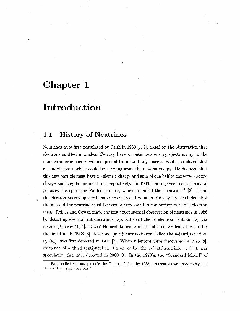
1.1 History of Neutrinos
Neutrinos were first postulated by Pauli in 1930 [1, 2], based on the observation that
electrons emitted in nuclear /3-decay have a continuous energy spectrum up to the
monochromatic energy value expected from two-body decays. Pauli postulated that
an undetected particle could be carrying away the missing energy. He deduced that
this new particle must have no electric charge and spin of one half to conserve electric
charge and angular momentum, respectively. In 1933, Fermi presented a theory of
/3-decay, incorporating Pauli's particle, which he called the "neutrino"1 [3]. From
the electron energy spectral shape near the end-point in /3-decay, he concluded that
the mass of the neutrino must be zero or very small in comparison with the electron
mass. Reines and Cowan made the first experimental observation of neutrinos in 1956
by detecting electron anti-neutrinos, ues, anti-particles of electron neutrino, ue, via
inverse /?-decay [4, 5]. Davis' Homestake experiment detected ues from the sun for
the first time in 1968 [6]. A second (anti) neutrino flavor, called the fx~ (anti) neutrino,
Vn (Vfi), was first detected in 1962 [7]. When r leptons were discovered in 1975 [8],
existence of a third (anti)neutrino flavor, called the r-(anti)neutrino, vT (vT), was
speculated, and later detected in 2000 [9]. In the 1970's, the "Standard Model" of
1Pauli called his new particle the "neutron", but by 1933, neutrons as we know today had claimed the name "neutron."
1
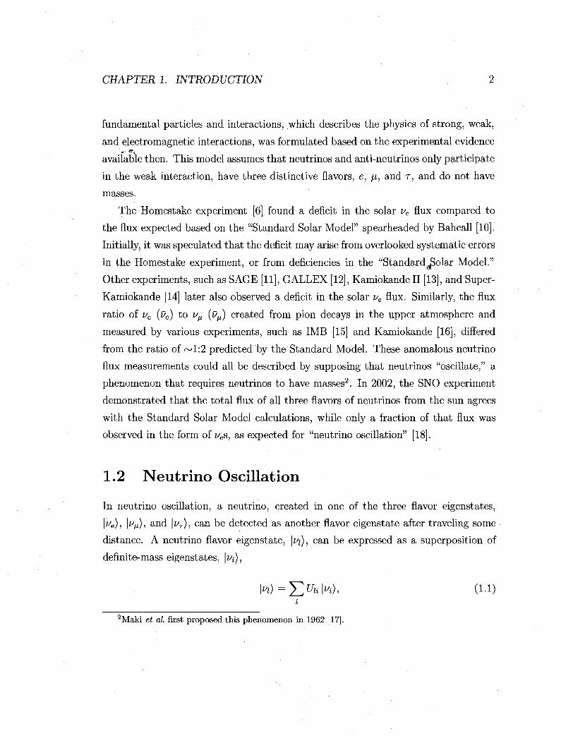
CHAPTER 1. INTRODUCTION 2
fundamental particles and interactions, which describes the physics of strong, weak,
and electromagnetic interactions, was formulated based on the experimental evidence
available then. This model assumes that neutrinos and anti-neutrinos only participate
in the weak interaction, have three distinctive flavors, e, //, and r , and do not have
masses.
The Homestake experiment [6] found a deficit in the solar i/e flux compared to
the flux expected based on the "Standard Solar Model" spearheaded by Bahcall [10].
Initially, it was speculated that the deficit may arise from overlooked systematic errors
in the Homestake experiment, or from deficiencies in the "StandardJ3olar Model."
Other experiments, such as SAGE [11], GALLEX [12], Kamiokande II [13], and Super-
Kamiokande [14] later also observed a deficit in the solar ue flux. Similarly, the flux
ratio of ue (pe) to v^ (z?M) created from pion decays in the upper atmosphere and
measured by various experiments, such as 1MB [15] and Kamiokande [16], differed
from the ratio of ~1:2 predicted by the Standard Model. These anomalous neutrino
flux measurements could all be described by supposing that neutrinos "oscillate," a
phenomenon that requires neutrinos to have masses2. In 2002, the SNO experiment
demonstrated that the total flux of all three flavors of neutrinos from the sun agrees
with the Standard Solar Model calculations, while only a fraction of that flux was
observed in the form of i^es, as expected for "neutrino oscillation" [18].
1.2 Neutr ino Oscillation
In neutrino oscillation, a neutrino, created in one of the three flavor eigenstates,
We), WIJ)I a n d Wr)i c a n be detected as another flavor eigenstate after traveling some
distance. A neutrino flavor eigenstate, Wi)i c a n be expressed as a superposition of
definite-mass eigenstates, Wi),
Wi) = ^UH\ui), (1.1)
i
2Maki et al. first proposed this phenomenon in 1962 [17].

CHAPTER 1. INTRODUCTION 3
where Uu is a unitary mixing matrix that can be parameterized with three mixing
angles, 0i2, 023, and #13, a CP violating phase, <5, and two Majorana phases, a.\ and
(1.2)
f uel
U^x
\uTl
ue2
U„2
UT2
O U& =
/ 1
0
UTS J \0
X
/
I
0
COS 6>23
- sin 023
COS #13
0
— sin 0 i3 e
0 \
sin #23
COS 023 /
0 sin013e"i<5 ^
1 0 s 0 cos013 j
X
cos012 sin 0i2 0 \
- sin 0i2 cos 0i2 0
V 0 o i y
/ eiai<2 0 0 N eia2/2 Q
V 0
0 0 )
In the ultra relativistic limit, the probability of a neutrino created in flavor eigen-
state \vi) to be detected in flavor eigenstate \ui>) after traveling a distance L through
vacuum is given by
PV^V{EV, L)=J2 I W*l2 + * ( E E UuU^U^e 2EV (1.3)
where Ara2j = |ra2 —m2| denotes the magnitude of the difference between the squares
of masses of mass eigenstates \ui) and \UJ), and Eu denotes the neutrino energy.
Using the experimental results indicating that A m ^ ^> A m ^ [19, 20], the ue survival
probability for a case where L is much larger than Ev/ Am%2 can be approximated by
PVe->Ve(E„, L) « sin4 0i3 + cos4 0i3 • 2„„ - 2 / ' l-27Am2 [eV2]L[mV sin2 20i2 sin2 ' 21 L J L J
Ev [MeV] (1.4)
CHAPTER 1. INTRODUCTION 4
Since #i3 is measured to be small [21], Equation 1.4 can be further simplified by the
approximation #13 <g; 1, which yields to zeroth order,
, n r , , . » „ . o /1.27Am2[eV2]L[m]\ P „ e ^ e ( ^ , L ) « l - sin2 2012 sin2 ^ E t /[Me V] J ' ( L 5 )
As one can see in Equation 1.5, neutrino oscillation can occur only if Am2,! is non
zero, i.e., at least one of the mass eigenstates must have a finite mass. Equation 1.5
can also be applied to the ue survival probability assuming CPT invariance. For more
details on the neutrino oscillation formalism, see [22].
1.3 Anti-Neutrino Sources
The two important Pe sources used in this thesis are nuclear reactors emitting ves
( reactors) from /?-decays following nuclear fission and radioactive decays inside the
Earth emitting ues (i>geos) from some /^-decays in the uranium and thorium decay
chains. The production mechanism of Reactors and ^Veo»3 cLI"6 explained in the following
sections.
1.3.1 Anti-Neutrinos from Nuclear Reactors
Nuclear reactors generate heat mostly from nuclear fission. Additional heat is gener
ated as the resulting fission fragments undergo a series of nuclear decays until they
become stable. Along with heat, the /^-decays of the fragments also produce ves.
More than 99.9% of Reactors are produced from the /?-decay following fission of only
four nuclei: 235U, 238U, 239Pu, and 241Pu [26].
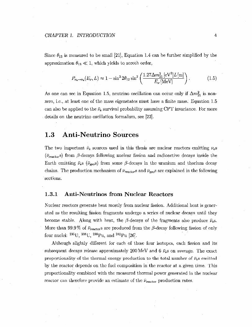
Although slightly different for each of these four isotopes, each fission and its
subsequent decays release approximately 200 MeV and 6 Pes on average. The exact
proport ional i ty of the thermal energy product ion to the to ta l number of v>es emit ted
by the reactor depends on the fuel composition in the reactor at a given time. This
proportionality combined with the measured thermal power generated in the nuclear
reactor can therefore provide an estimate of the i>reactor production rates.

CHAPTER 1. INTRODUCTION 5
^ 2i
§
>
«4H
o
-' J U L
E_ [MeV]
•« 0.6
o
0.2h
- I I I L .
2.5 -J 1 1 L.
3.5 E_ [Mevf
Figure 1.1: Top plot: energy spectra of ves from /3-decays following 2 3 5U (thin solid line) [23], 238U (thick dotted line) [24], 239Pu (thick solid line), and 241Pu (thin dotted line) [25] fission. Bottom plot: energy spectra of ues from 106Rh (solid line) and 144Pr (dotted line) /^-decays.

CHAPTER 1. INTRODUCTION 6
The top plot in Figure 1.1 shows the slight differences in the energy spectra of ves
from 235U, 238U, 239Pu, and 241Pu. The energy spectra of ves from 235U [23], 239Pu, and 241 Pu [25] are extracted from measurements of the /?-decay energy spectra of the fission
fragments after exposing each isotope to a thermal neutron flux for approximately
12 hours. The i>e energy spectrum for a single /?-decay branch is calculated using
the relation that the ue energy plus (3 energy equals the endpoint j3 energy of that
branch. However, neither the actual number of branches nor the amplitudes and
endpoint energies in the measured energy spectra of /^-decays following 235U, 239Pu,
and 241Pu fission are known. Therefore, each of the measured j3 energy spectra from
these isotopes is approximated by a combination of spectra from thirty hypothetical
/?-decay branches with some amplitude and endpoint energy. The Pe spectra from
all thirty hypothetical /?-decay branches are then added. On the other hand, the
energy spectrum of z/es from 238U is calculated theoretically up to 8MeV3 [24]. The
theoretically calculated energy spectra of ves from 235U, 239Pu, and 241Pu agree with
the measured spectra within ~10 %. Therefore a 10 % uncertainty is assumed for the
calculated energy spectrum of 9es from 238U. To calculate the total Reactor energy
spectrum from a nuclear reactor, the spectra from these isotopes need to be added
together and weighted according to the fuel composition of the reactor. The average
reactor flux uncertainty above the inverse /3-decay energy threshold (see Section 1.4)
from the spectral shape uncertainty is estimated to be 2.5 %.
Since the /3-decay energy spectra, from which the 235U, 239Pu, 241Pu ue spectra
are extracted, were measured after ~12 hours of exposure to a thermal neutron flux,
fragments with half-lives greater then a few hours had not yet reached equilibrium,
and therefore were not included in these spectra. Contributions from such "long-
lived" fragments are small, and mostly driven by 106Ru and 144Ce, with half-lives of
373.6 days and 284.9 days, respectively. Although the /^-decays of 106Ru and 144Ce
themselves do not produce i>es with high enough energy to be observed via inverse
/?-decay, the /?-decays of their daughters, 106Rh and 144Pr, do. The bottom plot in
Figure 1.1 shows the energy spectra of Pes produced in these decays.
3The contribution from the "missing" 238U Pe energy spectrum above 8 MeV to the total Preactor spectrum above 8 MeV is small since the fractional contribution of 238U fission in the reactor is typically less than 10 %.
CHAPTER 1. INTRODUCTION 7
o o
03
| l 0 2 0
p..
10
10
10
10
lfl
foooooooooooo
18
n
13
^ u a ^ " " " "
ooooooooo'
. . . . . . . . . . . . . . . . . . . . ooooooooc
235-
238-
239T T u A 2 4 % T 241T
242 'Pu o Pu •
T T T T " " T T T T T T TTTTTTT1
r T T T T TTTTTTTTTT^ r T T T M T » » »
FnannK . m l
a a a a a a u n u ^ ^ a nannaaaa
0 50 100 150 200 250 300 350 400 450 500 Days
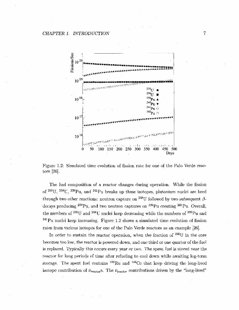
Figure 1.2; Simulated time evolution of fission rate for one of the Palo Verde reactors [26].
The fuel composition of a reactor changes during operation. While the fission
of 235U, 238U, 239Pu, and 241Pu breaks up these isotopes, plutonium nuclei are bred
through two other reactions: neutron capture on 238U followed by two subsequent /3-
decays producing 239Pu, and two neutron captures on 239Pu creating 241Pu. Overall,
the numbers of 235U and 238U nuclei keep decreasing while the numbers of 239Pu and 241Pu nuclei keep increasing. Figure 1.2 shows a simulated time evolution of fission
rates from various isotopes for one of the Palo Verde reactors as an example [26].
In order to sustain the reactor operation, when the fraction of 235U in the core
becomes too low, the reactor is powered down, and one third or one quarter of the fuel
is replaced. Typically this occurs every year or two. The spent fuel is stored near the
reactor for long periods of time after refueling to cool down while awaiting log-term
storage. The spent fuel contains 106Ru and 144Ce that keep driving the long-lived
isotope contribution of PreactorS- The Reactor contributions driven by the "long-lived"
CHAPTER 1. INTRODUCTION 8
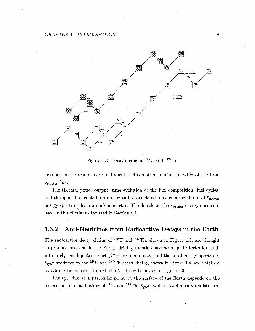
Figure 1.3: Decay chains of 238U and 232Th.
isotopes in the reactor core and spent fuel combined amount to ~ 1 % of the total
^reactor tlUX.
The thermal power output, time evolution of the fuel composition, fuel cycles,
and the spent fuel contribution need to be considered in calculating the total factor
energy spectrum from a nuclear reactor. The details on the Reactor energy spectrum
used in this thesis is discussed in Section 6.1.
1.3.2 Anti-Neutrinos from Radioactive Decays in the Earth
The radioactive decay chains of 238U and 232Th, shown in Figure 1.3, are thought
to produce heat inside the Earth, driving mantle convection, plate tectonics, and,
ultimately, earthquakes. Each /?~-decay emits a ue, and the total energy spectra of
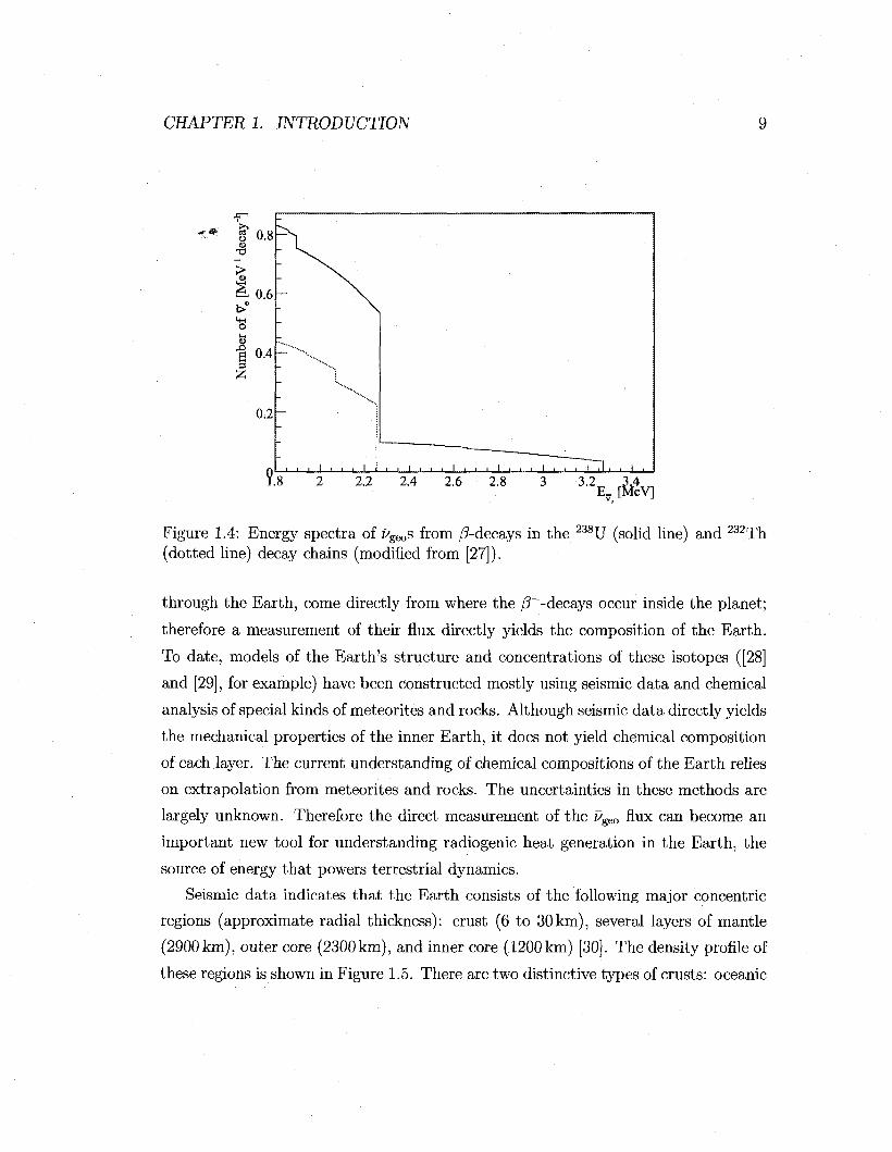
Pgeos produced in the 238U and 232Th decay chains, shown in Figure 1.4, are obtained
by adding the spectra from all the /?~-decay branches in Figure 1.3.
The £>geo flux at a particular point on the surface of the Earth depends on the
concentration distributions of 238U and 232Th. Pgeos, which travel mostly undisturbed
CHAPTER 1. INTRODUCTION 9
<**- I" 0.8 <U
^ 0.6
o t-l
I 0.4
0.2
9.8 ~2 ~2.2 2T4 Z6 ZS ~3~' 3Y 3A^ E_[MeV]
Figure 1.4: Energy spectra of z?geos from /^-decays in the 238U (solid line) and 232Th (dotted line) decay chains (modified from [27]).
through the Earth, come directly from where the /?~-decays occur inside the planet;
therefore a measurement of their flux directly yields the composition of the Earth.
To date, models of the Earth's structure and concentrations of these isotopes ([28]
and [29], for example) have been constructed mostly using seismic data and chemical
analysis of special kinds of meteorites and rocks. Although seismic data directly yields
the mechanical properties of the inner Earth, it does not yield chemical composition
of each layer. The current understanding of chemical compositions of the Earth relies
on extrapolation from meteorites and rocks. The uncertainties in these methods are
largely unknown. Therefore the direct measurement of the ugeo flux can become an
important new tool for understanding radiogenic heat generation in the Earth, the
source of energy that powers terrestrial dynamics.
Seismic data indicates that the Earth consists of the following major concentric
regions (approximate radial thickness): crust (6 to 30km), several layers of mantle
(2900 km), outer core (2300 km), and inner core (1200 km) [30]. The density profile of
these regions is shown in Figure 1.5. There are two distinctive types of crusts: oceanic
fx

CHAPTER 1. INTRODUCTION 10
u ra15
£• "55 c a> Q10
5
°<
"Upper -Mantle
-
. )
Lower Mantle
i
2000
Outer Core
i i I i i
4000
Inner Core
i 6000
Depth [km]
Figure 1.5: Density of the Earth as a function of the depth from the surface [28].
crusts, which are relatively young (~80 million years old) since they are constantly
renewed at the mid-ocean ridges and recycled back into the inner Earth at subduction
zones, and continental crusts, which are ~ 2 billion years old on average. Continental
crusts are thicker than oceanic crusts, and further subdivided into upper, middle,
and lower crusts. Sediment consisting of eroded continental crust and volcanic and
biological materials covers the surface of both the continental and oceanic crusts. The
composition of the sediment covering the continental crust is assumed to be the same
as that of the continental crust.
The chemical composition in each region has been studied with various meth
ods. Direct sampling of crusts is obtained from bore-holes. However, the deepest
bore-hole reaches only 12 km into the crust [31], approximately 0.2%, of the Earth's
radius. "Xenoliths," rock fragments brought up from the mantle to the surface in
lava flows without melting, give an indication of the chemical compositions of the
upper mantle. However, xenoliths are rare, and may not be a good representation
of the average mantle. These bore-hole and xenolith samples suggest that the crusts
and mantle are composed mainly of silica, and the crusts, especially the continental

CHAPTER 1. INTRODUCTION 11
crusts, contain high amounts of 238U and 232Th. A type of meteorite, type I carbona
ceous chondrite [32], is assumed to have the same composition of chemical elements
as the Earth did in its early formation stage, referred to as the "Bulk Silicate Earth
(BSE) [33]," in which the mantle and the crust had not yet been differentiated. The 238U and 232Th contents of the mantle is estimated by subtracting these contribu
tions from the crusts and sediment from the BSE. The core is believe to consist
of mostly iron, in which 238U and 232Th are insoluble4. Hence the concentrations of
these elements in the core are assumed to be negligible. Table 1.1 shows the estimated
concentrations of 238U and 232Th in each region based on the above studies [28]. The
mass ratio of 232Th to 238U, which chemical analyses of rocks and meteorites indicate,
lies between 3.7 and 4.1, more reliably estimated than the absolute concentrations in
each region [34].
Table 1.1: Estimated concentrations of 238U and 232Th in the major Earth regions [28].
Region
Oceanic sediment Oceanic crust Upper continental crust Middle continental crust Lower continental crust Mantle Core BSE
238 U [ppm] 1.68 0.10 2.8 1.6 0.2
0.012 0
0.02
232Th[ppm]
6.91 0.22 10.7 6.1 1.2
0.048 0
0.08
Based on the model, summarized in Table 1.1, the radiogenic power generation
from the decay chains of 238U and 232Th is estimated to be 16 TW. All the other ra
dioactive sources, mostly 40K, contribute an additional ~ 3 TW. On the other hand,
the total power dissipated from the Earth is estimated to be significantly higher than
the estimated radiogenic power generation. The total power dissipation of the Earth
is estimated to be 44.2 ± 1.0 TW by summing the heat flow measurements made
"Being lithophile elements with filled outer electron shells, 238U and 232Th form ionic bonds mainly with oxygen in silicates and oxides while metallic iron tends to bond with other transition metals.
CHAPTER 1. INTRODUCTION 12
in bore-holes and calculations based on empirical estimators derived from the ob
servations for unsurveyed areas and areas with hydrothermal effects5 [35]. A more
controversial approach, using only the heat flow measurements made in bore-holes
without the estimators that corrects for the hydrothermal circulation effects, yields
31 ± 1TW [36]. Although the exact mechanism is not known, the mantle is widely
believed to convect. Models of mantle convection suggest that the radiogenic heat
production rate should be the majority of the contribution to the Earth's heat dissi
pation rate [37, 38, 39]. Therefore if these models are correct, there is a discrepancy
between the total power dissipation estimation (44.2 ± 1.0 TW or 31 ± 1TW) and the
radiogenic power production estimation (~19TW). A measurement of the ugeo flux
can serve as an essential cross-check of the radiogenic power production estimation.
1.4 Anti-Neutrino Detection with KamLAND
KamLAND (Kamioka Liquid Scintillator Anti-Neutrino Detector) is a mineral-oil-
based liquid scintillator detector which detects &es via inverse /3-decay:
ue + p -^ e+ + n. (1.6)
A ue interacts with a proton, p, creating a positron, e+, and a neutron, n. The e+
quickly loses its kinetic energy in the scintillator by ionizing molecules and then an
nihilates with an electron, emitting two 0.511 MeV 7s6. Meanwhile, the n produced
in inverse /?-decay quickly thermalizes and is later captured by another p, creating
a 2.2 MeV 7 and a deuteron. The mean neutron capture time is ~200^s, and the
5 The heat flow measurements from many ocean floor areas are known to be biased too low due to the ocean water circulation removing the measurable heat [35].
6The e+ sometimes combines with an electron forming positronium (Ps) either in the para-Ps or ortho-Ps state [40]. The para-Ps state decays by emitting two 0.511 MeV 7s with a lifetime of 125 ps. In vacuum, the ortho-Ps state decays by emitting three 7s sharing total energy of 1.022 MeV with a lifetime of 140 ns. However, in matter, the majority of ortho-Ps interact with surrounding electrons and decay by emitting two 0.511 MeV 7s with a lifetime of a few ns. The three-7 decays of the ortho-Ps state produce slightly different amount of light in the detector from two-7 decays, which have the same total energy (see Section 3.4). This small effect is ignored, and e+ is always assumed to emit two 0.511 MeV 7s upon annihilation in this thesis.
CHAPTER 1. INTRODUCTION 13
a 1"
U
E* [MeV]
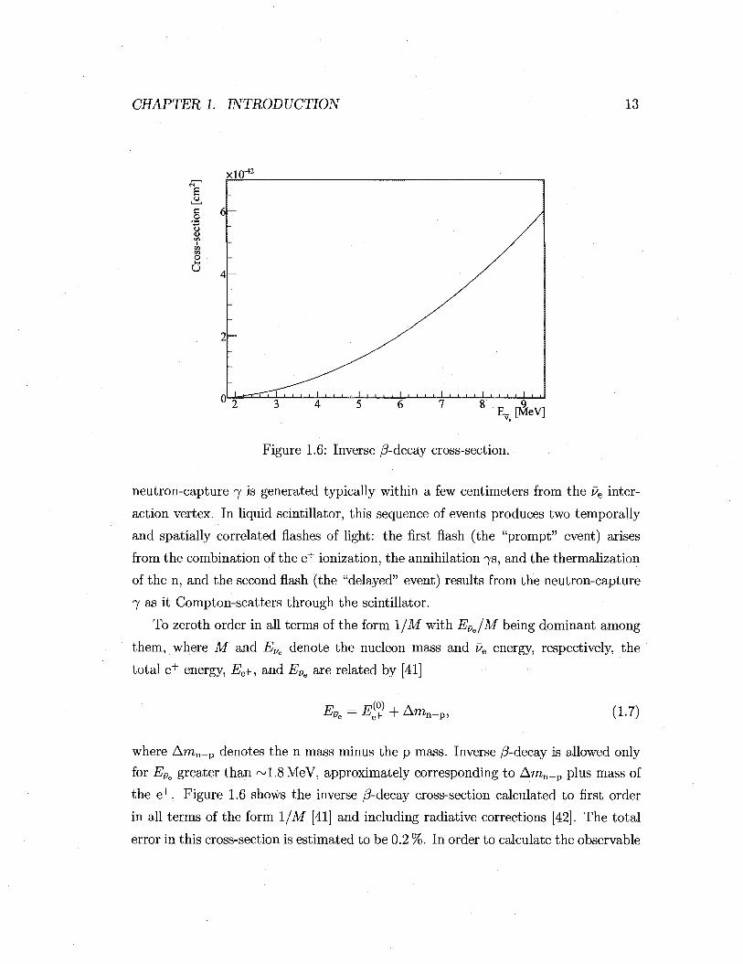
Figure 1.6: Inverse /3-decay cross-section.
neutron-capture 7 is generated typically within a few centimeters from the Pe inter
action vertex. In liquid scintillator, this sequence of events produces two temporally
and spatially correlated flashes of light: the first flash (the "prompt" event) arises
from the combination of the e+ ionization, the annihilation 7s, and the thermalization
of the n, and the second flash (the "delayed" event) results from the neutron-capture
7 as it Compton-scatters through the scintillator.
To zeroth order in all terms of the form 1/M with EPe/M being dominant among
them, where M and EDe denote the nucleon mass and ue energy, respectively, the
total e+ energy, Ee+, and EPe are related by [41]
EB_ = E® + Amn_p, Jve (1.7)
where Amn_p denotes the n mass minus the p mass. Inverse /?-decay is allowed only
for EDe greater than ~ 1.8 MeV, approximately corresponding to Aran_p plus mass of
the e+ . Figure 1.6 shows the inverse /?-decay cross-section calculated to first order
in all terms of the form 1/M [41] and including radiative corrections [42]. The total
error in this cross-section is estimated to be 0.2 %. In order to calculate the observable
CHAPTER 1. INTRODUCTION 14
is 1 /
* * / . ^
** / • " • - • A \ * / N \ •
* /' v \ * * /'' X% \ ** / / \ \ \
* / _ ^ * ^ ^ . x N. *
• / ^ ^v \ X •
*'// X. N-\ *\ •7/ X " \
f ^ X X 1 • • • • ' • • • • i • • • • i . . . . i . . . ^ T ^ ^ - I , !
2 3 . 4 5 6 7 8 _ __9 E_ [MeV]
IS
w 33
j i • •
E- [MeV]
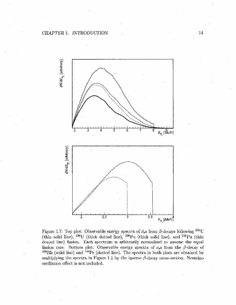
Figure 1.7: Top plot: Observable energy spectra of ves from /3-decays following 235U (thin solid line), 238U (thick dotted line), 239Pu (thick solid line), and 241Pu (thin dotted line) fission. Each spectrum is arbitrarily normalized to assume the equal fission rate. Bottom plot: Observable energy spectra of ves from the /?-decay of 106Rh (solid line) and 144Pr (dotted line). The spectra in both plots are obtained by multiplying the spectra in Figure 1.1 by the inverse /?-decay cross-section. Neutrino oscillation effect is not included.

CHAPTER 1. INTRODUCTION 15
J I I I I I I I I I I I I I I I I I I I I I I I I I I I LU I I L
1.8 2 2.2 2.4 2.6 2.8 3 3.2 3.4 E_ [MeV]
Figure 1.8: Observable energy spectra of ^geos from /^-decays in the 238U (solid line) and 232Th (dotted line) decay chains. This is obtained by multiplying Figure 1.4 by the inverse /?-decay cross-section.
EPe spectrum, this cross-section needs to be multiplied by the EPe spectrum of the
incident Pes. The raw energy spectra of ves produced in a nuclear reactor, shown in
Figure 1.1, and the Earth, shown in Figure 1.4, multiplied by the cross-section result
in the spectra shown in Figures 1.7 and 1.8, respectively.
1.5 Previous Measurements with KamLAND
The KamLAND collaboration published results on measurements of the neutrino os
cillation parameters, Am^ and sin22#i2, in 2003 [43] and 2005 [44], based on the
observation of Preactors from Japanese nuclear reactors. KamLAND separately con
ducted a study of ugeo in 2005 [45]; this was the first time ves were used as a tool for
geophysics.
These analyses were conducted using the "real energy7" spectra of prompt events,
- prompt* which consists of the kinetic energy of e+, two annihilation 7s, and neutron
7For details of real energy, see Section 3.4.
CHAPTER 1. INTRODUCTION 16
80
>
1 ' ' I ' ' " I " ' ' I ' ' ' ' I ' ' ' ' I ' " ' I " " I ' ' — — no-oscillation
accidentals 13C(a,n)160 spallation best-fit oscillation + BG KamLAND data
Ereal ,(MeV) prompt v '
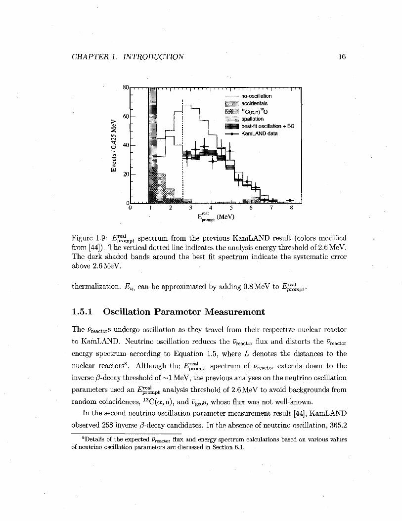
Figure 1.9: E™fmpt spectrum from the previous KamLAND result (colors modified from [44]). The vertical dotted line indicates the analysis energy threshold of 2.6 MeV. The dark shaded bands around the best fit spectrum indicate the systematic error above 2.6 MeV.
thermalization. EPe can be approximated by adding 0.8 MeV to E™fh prompt •
1.5.1 Oscillation Parameter Measurement
The Reactors undergo oscillation as they travel from their respective nuclear reactor
to KamLAND. Neutrino oscillation reduces the Preactor flux and distorts the Reactor
energy spectrum according to Equation 1.5, where L denotes the distances to the
nuclear reactors8. Although the E™fmpt spectrum of Reactor extends down to the
inverse /?-decay threshold of ~ 1 MeV, the previous analyses on the neutrino oscillation
parameters used an E^ t analysis threshold of 2.6 MeV to avoid backgrounds from
random coincidences, 13C(a:,n), and Pgeos, whose flux was not well-known.
In the second neutrino oscillation parameter measurement result [44], KamLAND
observed 258 inverse /?-decay candidates. In the absence of neutrino oscillation, 365.2
8Details of the expected factor flux and energy spectrum calculations based on various values of neutrino oscillation parameters are discussed in Section 6.1.

CHAPTER 1. INTRODUCTION 17
10"
1 0 ° -
-
-
-_ -
1
Solar
95% C.L. —- 99% C.L.
99.73% C.L. » solar best fit
>
~ l l • •
1 1 M i l
W ^ K.miLAND
95% C.L. g | | | 99% C.L.
H H 99.73% C.L. • KamLAND best fit
i i i
IO-1 10
tan26 12
Figure 1.10: Neutrino oscillation parameter inclusion contours at different confidence levels.from the previous KamLAND result (colors modified from [44]). The filled contours are from an analysis using only KamLAND data. The solid, dashed, and dotted lines are from solar ue experiments.
± 23.7 event-pairs, which included 17.8 ± 7.3 background event-pairs, were expected.
This discrepancy between the observed and expected numbers of event-pairs con
firmed the disappearance of Preactor at a confidence level of 99.998%. Disregarding
the normalization, the observed E™^mpt spectrum disagreed with the shape of the
expected E™fmpt spectrum in the absence of neutrino oscillation at a confidence level
of 99.6%. Figure 1.9 shows the E^mpt distribution. The KamLAND data exhibits
a dip around 3 MeV relative to the no-oscillation expected spectrum. The neutrino
oscillation parameters were estimated from the normalization and distortion of the
• prompt spectrum, both of which depend on the absolute time due to the temporal
variation in the nuclear reactor operation.
Figure 1.10 shows the inclusion contour in the neutrino oscillation parameter
space, Amj! and tan2(912. The three regions allowed at the 99.73% confidence level
in the KamLAND-only analysis have been named as LMA0, LMAl, and LMA2 from
CHAPTER 1. INTRODUCTION 18
bottom to top, where LMA stands for Large Mixing Angle9. KamLAND data pre
ferred the LMAl region, and the LMAO and LMA2 regions were disfavored over the
LMA1 region at confidence levels of 97.5% and 98.0%, respectively. When com
bined with neutrino oscillation results of solar ue experiments under the assumption
of CPT invariance, this analysis gave A m ^ = 7 .9^1 x 10~5eV2 (KamLAND alone),
and tan2 012 = 0.40±&#.
1.5.2 i/geo Investigation
The absolute number of Pgeos detected by KamLAND was estimated by fitting the
- prompt spectrum in the low energy region, 0.9 MeV < E^mpt < 2.6 MeV, using the
energy spectral shapes of the expected Pgeos from 238U and 232Th decay chains (see
Figure 1.8). The Pgeos undergo neutrino oscillation as they travel to KamLAND from
where they are produced inside the Earth. Since the production points of vgeos are
spread out within the Earth, the sin2 ( -—JJMMIVI ) * e r m m Equation 1.5 averages
out to 0.5, and hence the Pgeo flux is reduced by 1 — 0.5sin22#i2. The Pgeo energy
spectral shapes do not change appreciably due to neutrino oscillation. Figure 1.11
shows the expected spectra of well as backgrounds. The fitted numbers of
Pgeos from 238U and 232Th decay chains are 3 and 18, respectively.
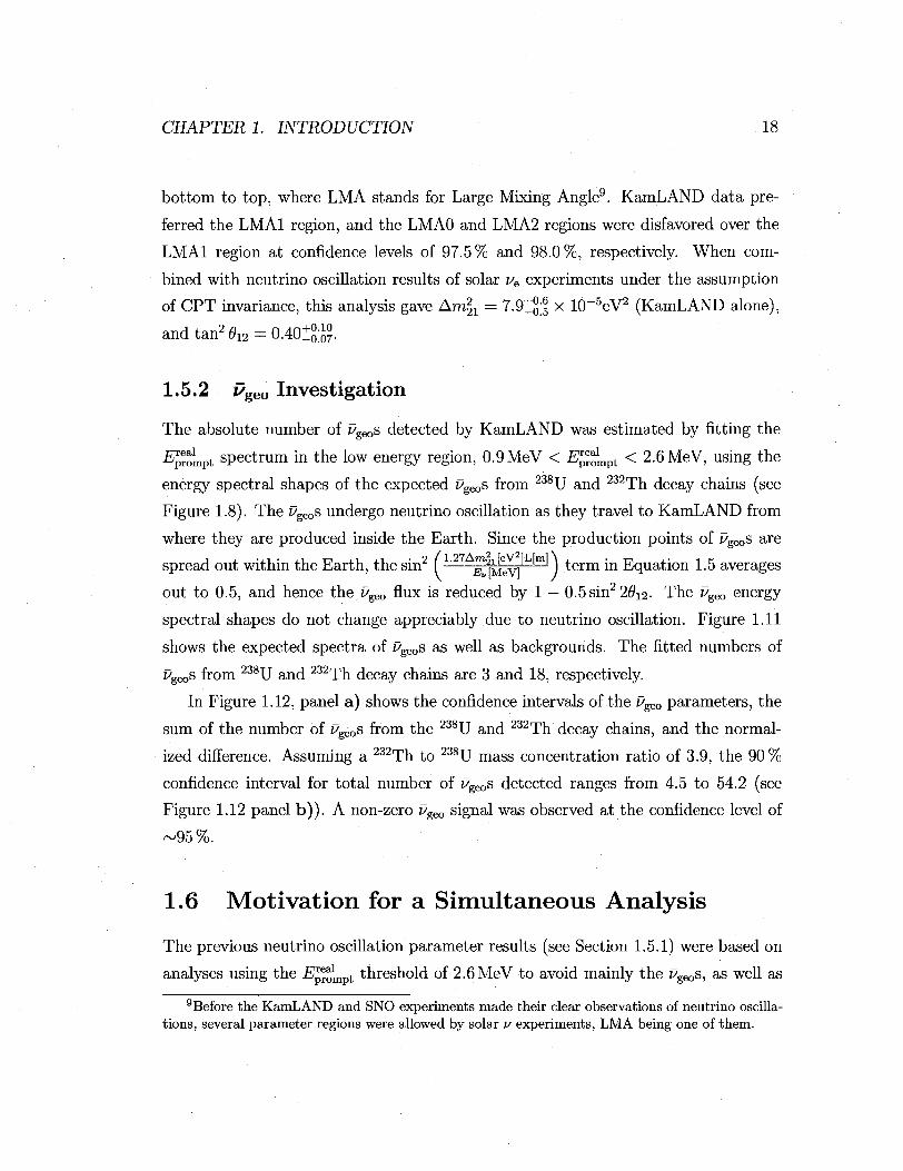
In Figure 1.12, panel a) shows the confidence intervals of the Pgeo parameters, the
sum of the number of Pgeos from the 238U and 232Th decay chains, and the normal
ized difference. Assuming a 232Th to 238U mass concentration ratio of 3.9, the 90 %
confidence interval for total number of Pgeos detected ranges from 4.5 to 54.2 (see
Figure 1.12 panel b)) . A non-zero Pgeo signal was observed at the confidence level of
- 9 5 % .
1.6 Motivation for a Simultaneous Analysis
The previous neutrino oscillation parameter results (see Section 1.5.1) were based on
analyses using the E™fmpt threshold of 2.6 MeV to avoid mainly the Pgeos, as well as
9Before the KamLAND and SNO experiments made their clear observations of neutrino oscillations, several parameter regions were allowed by solar v experiments, LMA being one of them.

CHAPTER 1. INTRODUCTION 19
5 N
2.2 2.4 2.6 2.8 3 Anti-neutrino energy, E (MeV)
Figure 1.11: The expected energy spectra of z/geos from 238U (thick dot-dashed line) and 232Th (thick dotted line) from the previous KamLAND result (colors modified from [45]) are based on the Earth model described in [28]. Expected spectra of factor (long dashed line), 13C(a,n) (thin dotted line), random coincidence (thin dot-dashed line), the total background (thick solid line), and the total events (thin solid line) are also shown. Panel a) shows the Pgeo candidate data (markers with error bars). In panel b), the expected spectra are extended to show the higher energy region.
backgrounds from random coincidences and 13C(o;,n). The separate ugeo study (see
Section 1.5.2), conducted with E™fmpt between 0.9MeV and 2.6MeV, treats Reactors
as background, and fixed the Reactor ^prompt spectral shape based on the neutrino
oscillation parameters obtained previously.
Instead of studying the neutrino oscillation parameters and ugeos separately, these
studies can be conducted simultaneously. Observing the full energy spectrum of
reactor should increase the sensitivity of the neutrino oscillation parameter measure
ment. By determining the factor spectrum more accurately, the Pgeo measurement
should also improve since factors are the largest background to the ugeo measurement.
Finally, a joint analysis will properly take into account for correlations between the
CHAPTER 1. INTRODUCTION 20
x <
1 1
1 1
1 1
1
1
!
I
/ JCL 35.4a
./......ix-sam
.1. jCLfia^a
»- "< -1 -0.5 0 0.5 1
OVny/flVNJ 20 40 60 80
V N T h
Figure 1.12: ugeo parameter results from the previous KamLAND study (colors modified from [45]). Panel a) shows the confidence level contours in the ugeo parameter space floating the ratio of ugeo contributions from 238U and 232Th. Panel b) shows the Ax 2 of the total number of ugeos observed with a fixed 232Th to 238U mass ratio of 3.9, estimated from other geophysical and planetary considerations. The gray boxes in both panel a) and b) indicate the expected Pgeos based on the Earth model described in [28].
fitted neutrino oscillation and vgeo parameters. This thesis pursues such a joint anal
ysis.
The analyses described in Section 1.5 were conducted using different Pe candidate
selection cuts. The candidate selection cuts for the ugeo study were much tighter
because of a large contribution from the random coincidence background at lower
energy. Combining these analyses and performing the fit simultaneously involves
consolidating the different candidate selection cuts.
The quantity E™fmpt used in the previous analyses is a rather unnatural unit
since it assumes that e+s cause the prompt events. However, prompt events from
background signals are not necessarily caused by e+s. These events and e+s would
have the same -Eprompt w n e n they produce the same amount of light in the detector.
A e + wi th no kinetic energy would yield t he minimum allowed £woLpt °f ~ 1 MeV.
Therefore the -E^ompt °f a background event that produces less light in the detector
does not correspond to any physical event involving e+s, and so is not well-defined.
To avoid these problems, the analysis presented in this thesis is conducted in terms

CHAPTER 1. INTRODUCTION 21
of the observable energy based on light yield.

CHAPTER 1. INTRODUCTION 22
Chapter 2
Detector
KamLAND (Kamioka Liquid scintillator Anti-Neutrino Detector) is located in a rock
cavern in the Kamioka mine, ~1000m below the summit of Mt. Ikenoyama in Gifu,
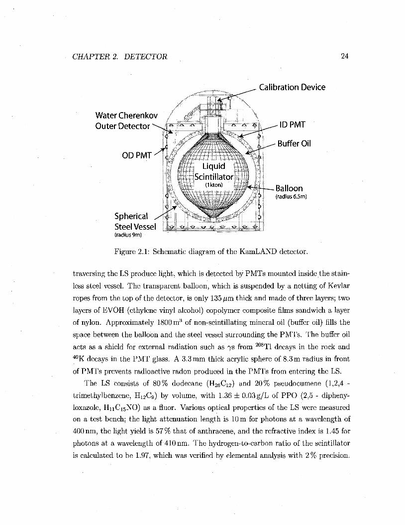
Japan. Mt. Ikenoyama shields the detector from cosmic rays. Figure 2.1 shows a
schematic of the detector, which consists of two major sections, the inner detector
(ID) and the outer detector (OD), separated by a spherical stainless steel vessel of 9 m
radius. The ID section is designed for detection of ues, and the OD section acts as a
cosmic ray active veto while also attenuating 7 radiation from the surrounding rock.
Light produced in the ID and OD is detected by photo multiplier tubes (PMTs), which
convert photons that hit their photo-cathodes into an electrical signal. Waveforms
from the PMTs, readout as voltage as a function of time, are recorded and later used
to reconstruct the energies and positions of events1. To test the performance of the
algorithms in finding the energy and position, radioactive calibration sources with
known energies are deployed at known positions.
2.1 Inner Detector
An approximately spherical balloon of 6.5 m radius is suspended inside the stainless
steel vessel and filled with 1171 ± 25 m3 of liquid scintillator (LS)2. Charged particles
1See Sections 3.2 and 3.3 for details of these algorithms. 2 The total volume of the LS was measured during detector filling.
23
CHAPTER 2. DETECTOR 24
Water Cherenkov Outer Detector ^ j ?
ODPMT
Calibration Device
IDPMT
Buffer Oil
Balloon (radius 6.5m)
Spherical Steel Vessel y„ y *y„„ „yj& v -^ *.y vJ (radius 9m)
Figure 2.1: Schematic diagram of the KamLAND detector.
traversing the LS produce light, which is detected by PMTs mounted inside the stain
less steel vessel. The transparent balloon, which is suspended by a netting of Kevlar
ropes from the top of the detector, is only 135 //m thick and made of three layers; two
layers of EVOH (ethylene vinyl alcohol) copolymer composite films sandwich a layer
of nylon. Approximately 1800 m3 of non-scintillating mineral oil (buffer oil) fills the
space between the balloon and the steel vessel surrounding the PMTs. The buffer oil
acts as a shield for external radiation such as 7s from 208T1 decays in the rock and 40K decays in the PMT glass. A 3.3 mm thick acrylic sphere of 8.3 m radius in front
of PMTs prevents radioactive radon produced in the PMTs from entering the LS.
The LS consists of 80% dodecane (H26Ci2) and 20% pseudocumene (1,2,4 -
trimethylbenzene, H12C9) by volume, with 1.36 ± 0.03 g/L of PPO (2,5 - dipheny-
loxazole, H11C15NO) as a fluor. Various optical properties of the LS were measured
on a test bench; the light attenuation length is 10 m for photons at a wavelength of
400 nm, the light yield is 57% that of anthracene, and the refractive index is 1.45 for
photons at a wavelength of 410 nm. The hydrogen-to-carbon ratio of the scintillator
is calculated to be 1.97, which was verified by elemental analysis with 2% precision.

CHAPTER 2. DETECTOR 25
The LS density was measured to be 0.778 g/m3 at 11.5 °C with 0.01% precision and
varies by 0.1 % due to variation of temperature within the detector. The LS density
is only 0.04% higher than that of the buffer oil (dodecane and isoparaffin) outside the
balloon, making the tension in the ropes and the balloon which enclose the scintillator
manageable. The liquid levels of the LS and the buffer oil are carefully monitored
to keep enough pressure inside the balloon to maintain the appropriate shape. To
reduce background radiation in both the LS and the buffer oil, commercially available
pure mineral oil and LS were purified with water extraction and nitrogen stripping
[46], achieving uranium, thorium, and potassium concentrations of 3.5 x 10~18g/g,
5.2 x 10~17g/g, and less than 2.7 x 10~16g/g, respectively. For more details on the
LS, see [47].
An array of 1325 Hamamatsu RS7250 17-inch-diameter PMTs3 and 554 Hama-
matsu R3600 20-inch-diameter PMTs, is mounted inside the stainless steel vessel
facing the center of the ID. The Hamamatsu RS7250 PMTs have better timing per
formance than the Hamamatsu R3600 PMTs. Also, 6 PMTs with 5-inch-diameter
look down to the ID from the top of the detector. In this analysis, only the data col
lected with the Hamamatsu RS7250 PMTs are used for the ID signal giving a total
photo-cathode coverage of approximately 22 %. These PMTs have a time resolution
of approximately 3 ns, and the quantum efficiency of the PMTs is approximately
20 % for photons with wavelengths between 340 and 400 nm. The observed number of
photo-electrons per MeV per PMT is approximately 0.2, therefore many PMTs ob
serve no photo-electrons for typical events in a few MeV range. For proper operation
of PMTs, a set of compensation coils encompassing the entire detector are used to
reduce the terrestrial magnetic field.
Three thermometers were initially attached at the top, center, and bottom of a
vertical line running slightly off the central axis of the detector. Radioactivity in the
line and especially the three thermometers produced background events; therefore the
line and thermometers were removed on April 19th, 2004. The periods before and
after this date are defined as "period I" and "period II," respectively.
3The diameter of these PMTs is actually 20 inches, but the photo-cathodes are masked down to 17-inch diameter to improve their transit-time spread.

CHAPTER 2. DETECTOR 26
2.2 Outer Detector
The OD is a cylindrical water-Cherenkov cosmic ray veto detector, which surrounds
the stainless steel vessel and contains approximately 3000 m3 of pure water. Hama-
matsu R3600 PMTs detect Cherenkov light produced by muons going through the
OD. The OD also acts as an attenuator for neutrons and 7s by reducing the number
of these particles entering the ID from outside the detector. The water in the OD is
circulated constantly to remove excess heat produced by PMTs in the ID and OD.
The OD has four sections: top, upper, lower, and bottom. The stainless steel
containment sphere separates the top and upper sections from the lower and bottom
sections. The PMTs in the top and bottom sections are attached on the ceiling and
the floor of the OD, facing downward and upward, respectively. The PMTs in the
upper and the lower sections are attached on the wall of the OD facing towards the
cylindrical axis of the detector. The top, upper, lower, and bottom sections contain
50, 60, 60, and 55 PMTs, respectively. Tyvek®4 plastic sheets optically separate each
section of the OD. These sheets are highly reflective and line all inner surfaces of the
OD to optimize light collection by the PMTs in each section.
2.3 Electronics and Data Acquisition
The system to record PMT data consists of three major components: the KamFEE
(KamLAND Front-End Electronics) system, which includes 200 KamFEE boards5,
the trigger system, and the DAQ (Data AcQuisition) system. The main purpose of
these components are that the KamFEE system acquires and digitizes PMT wave
forms, the trigger system decides whether to record the data, and the DAQ system
records the data. These three components communicate with each other as shown in
Figure 2.2. The DAQ system sends various commands to the trigger system, such as
run s ta r t and s top. The DAQ system also separately sends bo th the trigger system
4DuPont Tyvek® is a lightweight and durable material. 5Another set of redundant front-end electronics, called MACRO electronics, also record wave
forms. However, the waveforms recorded with the MACRO electronics are not analyzed in this thesis.
CHAPTER 2. DETECTOR 27
>
Run Conditions
'
Data
Trigger
DAQ Run Conditions
Data
Digitization Command and Clock w
^KamFEE 5
> t
KamFEE Charge
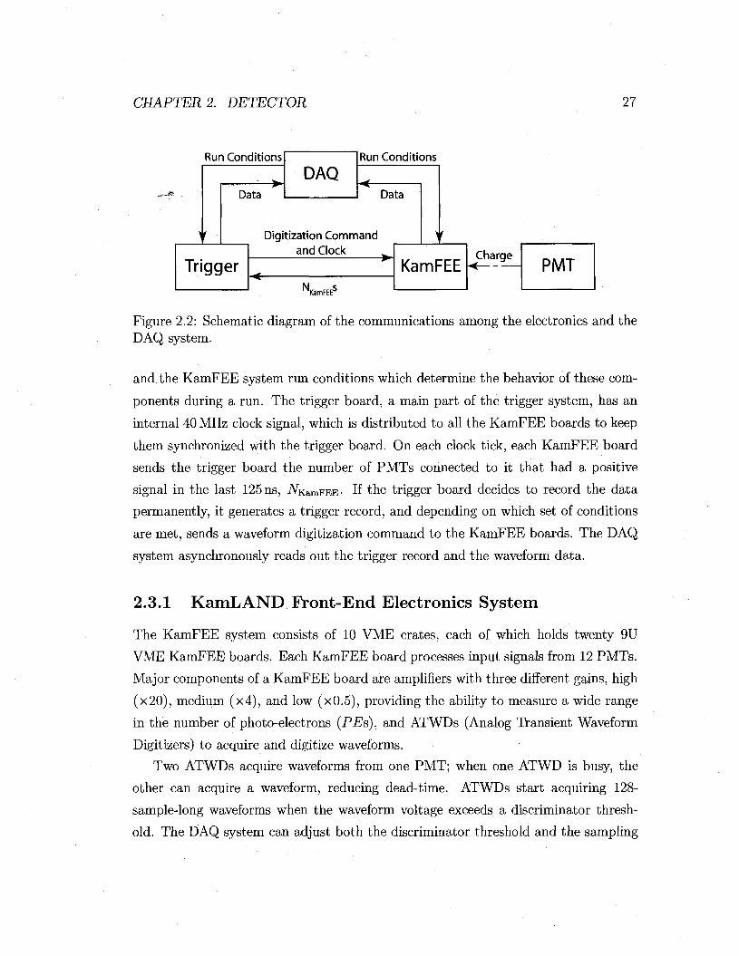
Figure 2.2: Schematic diagram of the communications among the electronics and the DAQ system.
and the KamFEE system run conditions which determine the behavior of these com
ponents during a run. The trigger board, a main part of the trigger system, has an
internal 40 MHz clock signal, which is distributed to all the KamFEE boards to keep
them synchronized with the trigger board. On each clock tick, each KamFEE board
sends the trigger board the number of PMTs connected to it that had a positive
signal in the last 125 ns, A amFEE- If the trigger board decides to record the data
permanently, it generates a trigger record, and depending on which set of conditions
are met, sends a waveform digitization command to the KamFEE boards. The DAQ
system asynchronously reads out the trigger record and the waveform data.
2.3.1 KamLAND Front-End Electronics System
The KamFEE system consists of 10 VME crates, each of which holds twenty 9U
VME KamFEE boards. Each KamFEE board processes input signals from 12 PMTs.
Major components of a KamFEE board are amplifiers with three different gains, high
(x20), medium (x4), and low (x0.5), providing the ability to measure a wide range
in the number of photo-electrons (PEs), and ATWDs (Analog Transient Waveform
Digitizers) to acquire and digitize waveforms.
Two ATWDs acquire waveforms from one PMT; when one ATWD is busy, the
other can acquire a waveform, reducing dead-time. ATWDs start acquiring 128-
sample-long waveforms when the waveform voltage exceeds a discriminator thresh
old. The DAQ system can adjust both the discriminator threshold and the sampling

CHAPTER 2. DETECTOR 28
frequency. The sampling frequency for a normal run is typically set to approximately
0.65 GHz, making the length of a waveform approximately 200 ns. Each ATWD
has 4 inputs and can simultaneously acquire 4 independent waveforms. The three
waveforms from one PMT, after three different amplifications, use three of the four
available ATWD inputs. A sinusoidal waveform derived from the 40 MHz clock signal
feeds the remaining ATWD input and is used to calibrate the sampling time.
After completing the acquisition of waveforms, the ATWDs hold them for a pre
determined duration of time, which is set to be 175 ns during a normal run. By the
end of this time, if the KamFEE boards have not received the digitization command
from the trigger board, the acquired waveforms are erased within approximately 1 fis,
making the ATWDs available to acquire more waveforms. Alternatively, if the Kam
FEE boards receive a digitization command, they digitize the acquired waveforms
with a 10-bit ADC, which takes approximately 30 //s. Waveforms in all three gains
are recorded for high energy interactions such as muons going through the detector
since the amplitudes of the high and medium gain waveforms for such events typically
saturate the 10-bit ADC. On the other hand, only the waveforms in the high gain
ATWD channels are recorded for events with energy in the MeV range, which provides
less than a few photons per PMT. Each waveform is associated with a timestamp of
when the KamFEE board received the digitization command from the trigger board,
where timestamp is the number of clock ticks since the beginning of the run. The
timestamp is used later to associate all the different waveforms and the trigger record
from the same event. Each waveform also has an associated launch offset value, which
is the number of clock ticks between when the ATWD started acquiring a waveform
and when it received the digitization command from the trigger board.
2.3.2 Trigger Electronics System
The main components of the trigger system are a custom-built trigger processor board
(trigger board) and a variety of ancillary components housed in a VME crate (trigger
VME crate). The trigger board communicates with the DAQ system through mod
ules in the trigger VME crate. The trigger command and clock signal are distributed

CHAPTER 2. DETECTOR 29
to the KamFEE boards through other modules also in the trigger VME crate. In
case the main DAQ system becomes overwhelmed due to high data rates, caused by
a supernova explosion6 for example, the trigger record is duplicated and indepen
dently recorded by the trigger backup DAQ system. For more information on the
trigger backup DAQ system and the trigger system VME modules, see Appendix A.
The trigger board also communicates with the absolute-time acquisition system (see
Appendix C). This would be important in order to compare observations by Kam-
LAND with those of other experiments in case of a global event, such as a supernova
explosion.
The trigger board decides whether the data should be recorded. The conditions
on which this decision is made are referred to as the "trigger type." For details on
the various trigger types, see [27] and Appendix B. This decision is based on the
enabled trigger types and thresholds, and the sum of all the ArKampEES in each section
of the detector7: in the ID (Aro)8, OD top (AoDtop), OD upper (AoDupper), OD lower
(A^oDiower), OD bottom (AoDbottom), and the chimney (A5»). When the trigger board
decides to record the data, it produces a trigger record consisting of the timestamp,
the trigger type, and the values of Nm, AODtop, AODupper, A ODiower, AODbottom, and
AV.
During normal data taking, the trigger board sends a digitization command to the
KamFEE boards most often via a "prompt" trigger, defined to occur when AID goes
above a threshold, set to 200 or 180, before and after April 13th, 2004, respectively.
Similarly, the trigger board sends a digitization command to the KamFEE boards for
each section of the OD when AODtoP, AODupper, A0Diower, or AoDbottom goes over their
respective thresholds. The trigger board sends the digitization commands back to
KamFEE boards within ~400 ns from the time KamFEE boards calculate AKamFEES,
on which the trigger board based its decision.. This timing specification ensures the
digitization commands to reach the KamFEE boards before they erase the acquired
6A typical supernova explosion is expected to produce a burst of neutrino events lasting for a few seconds.
7Although most of the decisions to record data are based on A KamFEES, some are strictly based on timing, such as the lpps trigger and GPS trigger. For more details on trigger types, see [27] and Appendix B.
sNir> does not include the number of Hamamatsu R3600 PMTs with a photon-hit in the ID.

CHAPTER 2. DETECTOR 30
waveforms. Some trigger types do not send a digitization command to KamFEE
boards. The trigger board issues a "history" trigger, for instance, when A^D goes
above a history trigger threshold, usually set to 120, and while it remains above
threshold for up to 8 consecutive clock ticks to keep track of the time evolution of iVm.
There are similar "OD history" triggers for each section of the OD. More detailed
information on the trigger electronics system is available in [27], and Appendix A.
2.3.3 DAQ System
The main tasks of the DAQ system are to set run conditions for the trigger system
and the KamFEE system, to readout the data from these systems, to record them
on the data storage disk, and to provide the user interface for run control and config
uration. The DAQ software used for the KamLAND experiment is called KiNOKO
(KiNOKO is Network distributed Object oriented KamLAND Online system). Ki
NOKO is a networked parallel processing system installed on 15 front-end computers,
which asynchronously read data from 15 VME crates (10 for reading out all KamFEE
boards, 1 for the trigger system, and 4 for the MACRO electronics9). The data is
then transfered to a back-end computer which is also controlled by KiNOKO. In this
back-end computer, KiNOKO performs a simple online analysis on the readout data.
The data flow rate from each VME crate, for example, is calculated at this stage.
Another important quantity that KiNOKO calculates is NuaxiD, defined to be the
maximum NiD in the consecutive trigger records obtained via history triggers in an
event. Similarly, KiNOKO also calculates the maximum AoDtop, - ODupper, -NoDiower
and A oDbottom using history triggers for the corresponding OD section. After calcula
tions of these and other quantities, KiNOKO displays them in histograms and graphs,
which can be used to monitor data taking realtime. A detector operator can start
or stop a run through KiNOKO, where a run is a period of continuous data taking
typically lasting 24 hours. During a run start procedure, the electronics devices are
configured through KiNOKO. For more details on KiNOKO, see [28].
9Another set of redundant front-end electronics that are not used in this thesis.
CHAPTER 2. DETECTOR 31
2.4 Detector Calibration
Radioactive sources with known energies are deployed into the ID through a small
opening in the ID chimney. Before December 2005, all deployments were performed
along the central vertical axis (z-axis) of the detector, and the positions of the ra
dioactive sources along this axis were known within a few mm. In December 2005, a
so-called "4-7r" system was commissioned, which can deploy radioactive sources at po
sitions away from the vertical axis. The 4-7r system deploys pole segments connected
to form a straight shaft. The number of pole segments and the angle at which the
pole is deployed can be adjusted. Each pole segment is equipped to hold a radioactive
source. Although the absolute position of the poles, and therefore the sources, are not
precisely known, the distances between the sources in the pole segments are known
to within a few mm.
The energies and types of radioactive sources which have been deployed in the ID
are listed below:
• 203Hg produces 0.279 MeV 7s.
• 68Ge produces e+s, each of which annihilates with an e~ inside the source con
tainment capsule producing two 0.511 MeV 7s.
• 65Zn produces 1.116 MeV 7s.
• 60Co produces two 7s at 1.173 MeV and 1.332 MeV in very short temporal co
incidence.
• 60Co68Ge is a composite source that contains 60Co and 68Ge in the same cap
sule. To reduce the detector dead-time and the risk of introducing radioactive
impurity in the detector due to calibration runs, these sources are combined
and deployed together.
• 241Am9Be produces mainly three types of events [48]:
— Neutrons with kinetic energies between ~5.5 and ~ H M e V .

CHAPTER 2. DETECTOR 32
— Pairs of a 4.439 MeV 7 and a neutron with kinetic energy between ~1.5
and ~6.5 MeV, emitted simultaneously.
— A 4.439 MeV 7, a 3.215 MeV 7, and a neutron with kinetic energy below
~ 3 MeV, emitted simultaneously.
The neutrons produced from the 241Am9Be source in the LS lose their kinetic
energy primarily via elastic scattering with protons. The scattered protons produce
scintillation light in the LS, that is quenched because of the high ionization density
(see Section 3.4). If the neutrons have enough energy, they can also lose energy
via inelastic scattering on 12C in the LS, which produces 4.439 MeV 7s. The free
neutrons eventually capture on protons or 12C, producing 2.223 MeV and 4.945 MeV
7s, respectively.

Chapter 3
Event Reconstruction
The light produced in the ID by scintillation and Cherenkov radiation from ionizing
particles and muons is viewed by the PMTs. The energies and positions of point-like
events or muon tracks must be calculated from these PMT signals. The first step
in reconstructing events is to associate all of the asynchronously read-out waveforms
and the trigger record with the same timestamp as an event. This is performed
offline in software. After all the information from each event is grouped, the pulses
in the waveforms are identified, and their times and charges are calculated. These
times and charges are then used by the position, energy, and muon track finding
algorithms. These algorithms are tested using various methods, typically based on
deployed radioactive sources or naturally occurring radioactivity in the detector.
3.1 Pulse Time and Charge
The arrival time and charge of pulses are extracted from each waveform in an event
using two different methods; the Small Pulse Analyzer (SPA), ideal for waveforms
containing small pulses from low energy events, and the Large Pulse Analyzer (LPA),
ideal for waveforms containing large pulses from muons.
At the beginning of a run, 50 waveforms from all ATWDs are recorded at a
fixed frequency, rather than based on iNfo, and are therefore unlikely to contain
any pulses. From these "empty" waveforms, fixed fluctuations characteristic to each
33
CHAPTER 3. EVENT RECONSTRUCTION 34
§150
100
50
0
0 20 40 60 80 100 120 ATWD sample
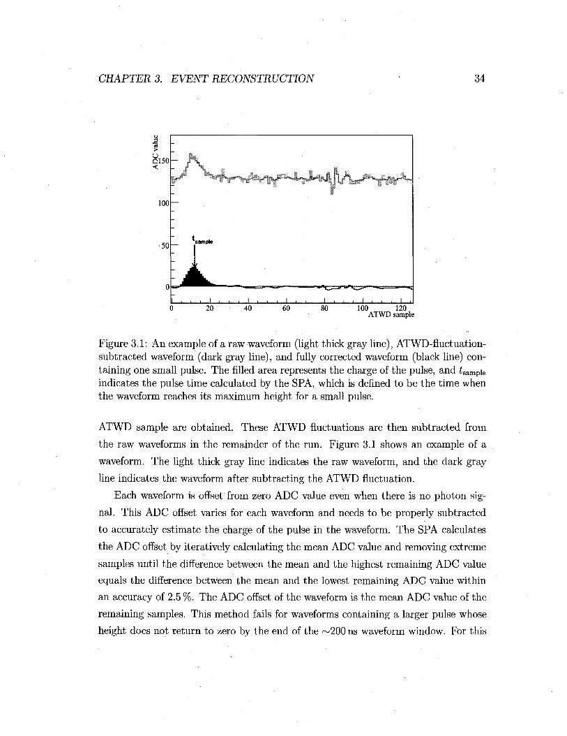
Figure 3.1: An example of a raw waveform (light thick gray line), ATWD-fluctuation-subtracted waveform (dark gray line), and fully corrected waveform (black line) containing one small pulse. The filled area represents the charge of the pulse, and Sample indicates the pulse time calculated by the SPA, which is defined to be the time when the waveform reaches its maximum height for a small pulse.
ATWD sample are obtained. These ATWD fluctuations are then subtracted from
the raw waveforms in the remainder of the run. Figure 3.1 shows an example of a
waveform. The light thick gray line indicates the raw waveform, and the dark gray
line indicates the waveform after subtracting the ATWD fluctuation.
Each waveform is offset from zero ADC value even when there is no photon sig
nal. This ADC offset varies for each waveform and needs to be properly subtracted
to accurately estimate the charge of the pulse in the waveform. The SPA calculates
the ADC offset by iteratively calculating the mean ADC value and removing extreme
samples until the difference between the mean and the highest remaining ADC value
equals the difference between the mean and the lowest remaining ADC value within
an accuracy of 2.5 %. The ADC offset of the waveform is the mean ADC value of the
remaining samples. This method fails for waveforms containing a larger pulse whose
height does not return to zero by the end of the ~200 ns waveform window. For this
< * ™ * * * W * * * W ^ * H ^ ' ~ ~ ' < * ° ~ * * - - « ~ I J $ ^ ^ f l ^s^]rfw*^*"*~**~*««*&n»*~*''*~'"
sample
I . . . I i • • I i . . I . . i I . . . I

CHAPTER 3. EVENT RECONSTRUCTION 35
reason, the LPA calculates the ADC offset by taking the mean of the first 10 ATWD
samples, which are unlikely to contain a pulse. For both the SPA and the LPA, after
the ADC offset is subtracted from the ATWD-fluctuation-subtracted waveform, it is
smoothed using a Savitzky-Golay filter [49], which removes high frequency compo
nents while tending to preserve the maxima, the minima, and the width. The black
line in Figure 3.1 shows an example waveform after all of these corrections are applied.
Next, "pulses" are defined, and their charges and times are extracted. The SPA
defines each contiguous area above zero as a pulse as long as that area is greater
than 15% of the waveform's total area above zero. The 15% cut is chosen to reduce
misidentification of noise as pulses. The LPA defines the entire waveform to be one
pulse.
The area of each pulse gives a measure of its charge, in units of ADC value x
ATWD samples. To avoid underestimating the charge of a pulse by using a waveform
with a truncated amplitude, the charge of a pulse is calculated using the corrected
waveform from the lowest gain recorded for a particular signal. To calculate the
number of PEs, the charge is divided by the 1 PE equivalent charge (q0) of each
ATWD obtained from calibration runs with the 60Co source deployed at the center
of the detector. The q0s are updated every few weeks.
The total PEs in an event is defined as NPE1D, and the RMS of PMT-to-PMT
PE variation, RMSPEYD, is.given by
RMSPEID
\ E ^ -r)] • (3-D
where N denotes the number of PMTs with at least one pulse, PEX denotes the PE
of the ith PMT, and (PE) denotes the average PE for all PMTs with at least one
pulse in the event. These two variables, NPEID and RMSPEID, a r e used to classify
event types, particularly muons (see Section 3.6).
The times of pulses are always calculated from the waveforms from the high gain
since this provides consistency across the wide range of signal amplitudes. The SPA
defines the time of a pulse, Sample, in units of number of ATWD samples from the start

CHAPTER 3. EVENT RECONSTRUCTION 36
of the waveform, to be the peak of the second-order polynomial fit to the corrected
waveform from the lowest gain recorded for a particular signal. On the other hand,
the LPA defines the time of a pulse to be the time when the corrected waveform from
the high gain crosses 50 ADC value. Since each waveform in an event can be recorded
at different time, the pulse time needs to be given with respect to the arrival of the
trigger command, which should be the same for all ATWDs. The sampling durations
differ slightly among all the ATWDs, so actual duration between the beginning of
the waveform and the time of a particular sample differ depending on the ATWDs.
The relative timing of each pulse with respect to the time of the trigger command is
given by
Relative [ns] = 4ampie x psampie [ns/sample] - iViaUnch x 25 ns + t0 [ns], (3.2)
where pSampie denotes the duration of one ATWD sample in ns, Aiaunch denotes the
launch offset (see Section 2.3.1), and to denotes the timing correction for each ATWD
due to the signal travel time differences caused by slight differences in each cable
length or behavior in each KamFEE channel. pSamPie is calibrated for each ATWD at
the start of each run using the 40 MHz clock signal feed into the fourth ATWD input
as described in Section 2.3.1. to for each ATWD is measured with the 60Co source
deployed at the center of the detector and updated every few weeks.
3.2 Position Reconstruction
The event position is reconstructed in two major steps; a rough estimation is made
using the PE distribution among the PMTs, then fine tuning is done using the times
that the photons take to travel in a straight line from the event position to the PMTs.
The times and PEs of the pulses used in these steps are estimated with the SPA.
In the first step, the rough estimation of the event position is calculated from the
average of all the PMT positions weighted by the PEs, and the estimated position
vector from the center of the detector is multiplied by the empirical correction factor of
1.62. The factor 1.62 is chosen by comparing the estimated positions with the actual

CHAPTER 3. EVENT RECONSTRUCTION 37
positions of the 60Co source deployed along the vertical central axis of the detector.
Due to this factor, events at large radius are sometimes estimated to be outside of the
ID by this first step. If the estimated radius exceeds 8.5 m, the estimated position is
forced to the radius of 8.5 m in the same direction with respect to the center of the
ID.
During the second step, the event position is fine-tuned in multiple iterations. The
event position is adjusted using
Ot = tarrival Hraveh V"-'-'/
the difference between the actual photon arrival time, ^arrival, a n d the estimated photon
travel time travel? f° r the current estimated event position, travel is calculated using
the effective speeds of light in the LS and buffer oil of 196.1 mm/ns and 220mm/ns,
respectively. These effective speeds of light are empirically adjusted to minimize
the reconstructed position bias for radioactive sources deployed along the central
vertical axis. The index of refraction measured to be 1.45 as described in Section 2.1
corresponds to a phase velocity of 207mm/ns. However, PMTs detect individual
photons that propagate at the wave-packet group velocity, approximately 195 mm/ns.
This group velocity is close to the adjusted effective speed of light in the LS. The
accuracy of the reconstructed positions is much more sensitive to the effective speed
of light in the LS than that in the buffer oil. The difference between the measured and
the adjusted effective speed of light in the buffer oil might be due to the inaccuracy in
the model used in the position reconstruction algorithm, such as ignoring refraction
at the boundary between the LS and the buffer oil.
The algorithm uses photons most of which reach the PMTs directly, i.e., without
absorption and re-emission, by selecting pulses in a 15 ns window around the peak of
St distribution, as shown in Figure 3.2. During each iteration, the estimated event
position is pushed by a distance in a direction that reduces the width of the 6t
distribution in this 15 ns peak window. The event position reconstruction algorithm
has seven possible exit statuses for each event, "valid" for a successful fit, and six
other statuses for a fit that failed for various reasons, such as too few pulses in the

CHAPTER 3. EVENT RECONSTRUCTION 38
g200|
-100 8t [ns]
Figure 3.2: An example of the 5t distribution for an event. The position finding algorithm uses the pulses between the thin vertical dotted lines. The thick vertical dotted line indicates the mean 6t of these pulses.
event. Most of the events with a failed position reconstruction are caused by very-
low energy point-like events which do not produce enough photons or noise caused by
muons, such as after-pulses in the PMTs and multiple signal reflections in the PMT
cables. For more details on the position reconstruction algorithm, see Appendix D.
The performance of the event position finding algorithm is evaluated with radioac
tive sources, with energies in the range of ~ l M e V to ~5MeV, deployed at various
known positions from -5.5 m to 6 m along the central vertical axis. Figure 3.3 shows
the biases and RMS's of the reconstructed positions in the vertical direction for 68Ge, 65Zn, 60Co, and 241Am9Be. The biases for these sources within a 5.5 m radius along
the vertical axis are less than 5 cm, and the i?MS"s are within 30 cm.
The data from various source deployments off the vertical axis using the 4-7T system
confirm that the reconstructed position biases at various radii and angles from the
center of the detector are all less than ~ 5 cm within the fiducial volume radius of
5.5 m (see Section 5.3.3). For more details on the A-ir calibration results, see [50].
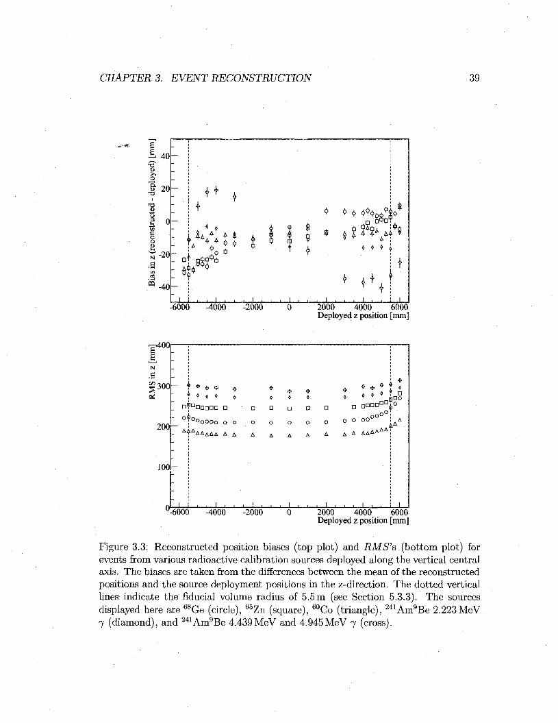
CHAPTER 3. EVENT RECONSTRUCTION 39
£, 40
-4000 2000 4000 6000 Deployed z position [mm]
^400:
N
.a 2300 _ *
2 0 0 -
100
. * « * ^ « 0 0 0 0 0
°i°00OOo O O
- A A AAA AAA A A
_L
* » * f o • * * * o§
o o oo"
A A A A A A AAT
-6000 -4000 -2000 2000 4000 6000 Deployed z position [mm]
Figure 3.3: Reconstructed position biases (top plot) and RMS's (bottom plot) for events from various radioactive calibration sources deployed along the vertical central axis. The biases are taken from the differences between the mean of the reconstructed positions and the source deployment positions in the z-direction. The dotted vertical lines indicate the fiducial volume radius of 5.5 m (see Section 5.3.3). The sources displayed here are 68Ge (circle), 65Zn (square), 60Co (triangle), 241Am9Be 2.223 MeV 7 (diamond), and 241Am9Be 4.439 MeV and 4.945MeV 7 (cross).
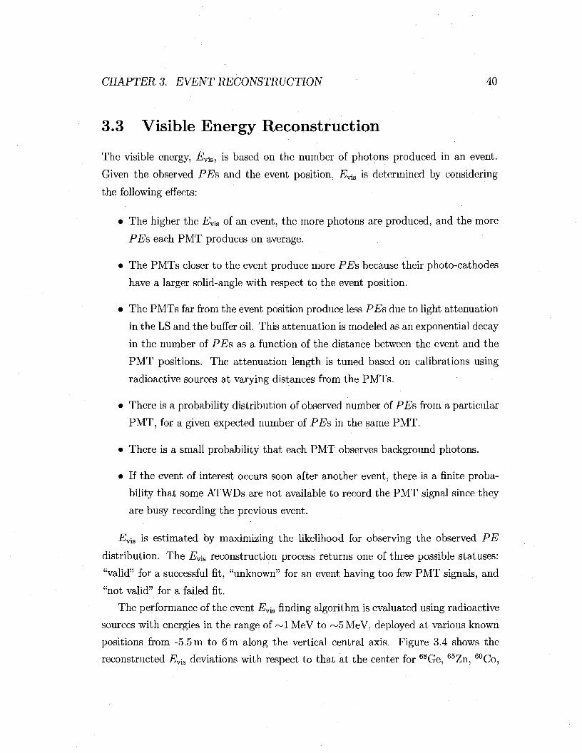
CHAPTER 3. EVENT RECONSTRUCTION 40
3.3 Visible Energy Reconstruction
The visible energy, EV{S, is based on the number of photons produced in an event.
Given the observed PEs and the event position, Evis is determined by considering
the following effects:
• The higher the Evis of an event, the more photons are produced, and the more
PEs each PMT produces on average.
• The PMTs closer to the event produce more PEs because their photo-cathodes
have a larger solid-angle with respect to the event position.
• The PMTs far from the event position produce less PEs due to light attenuation
in the LS and the buffer oil. This attenuation is modeled as an exponential decay
in the number of PEs as a function of the distance between the event and the
PMT positions. The attenuation length is tuned based on calibrations using
radioactive sources at varying distances from the PMTs.
• There is a probability distribution of observed number of PEs from a particular
PMT, for a given expected number of PEs in the same PMT.
• There is a small probability that each PMT observes background photons.
• If the event of interest occurs soon after another event, there is a finite proba
bility that some ATWDs are not available to record the PMT signal since they
are busy recording the previous event.
i?vis is estimated by maximizing the likelihood for observing the observed PE
distribution. The Evis reconstruction process returns one of three possible statuses:
"valid" for a successful fit, "unknown" for an event having too few PMT signals, and
"not valid" for a failed fit.
The performance of the event Ev\s finding algorithm is evaluated using radioactive
sources with energies in the range of ~ 1 MeV to ~5MeV, deployed at various known
positions from -5.5 m to 6 m along the vertical central axis. Figure 3.4 shows the
reconstructed Evia deviations with respect to that at the center for 68Ge, 65Zn, 60Co,
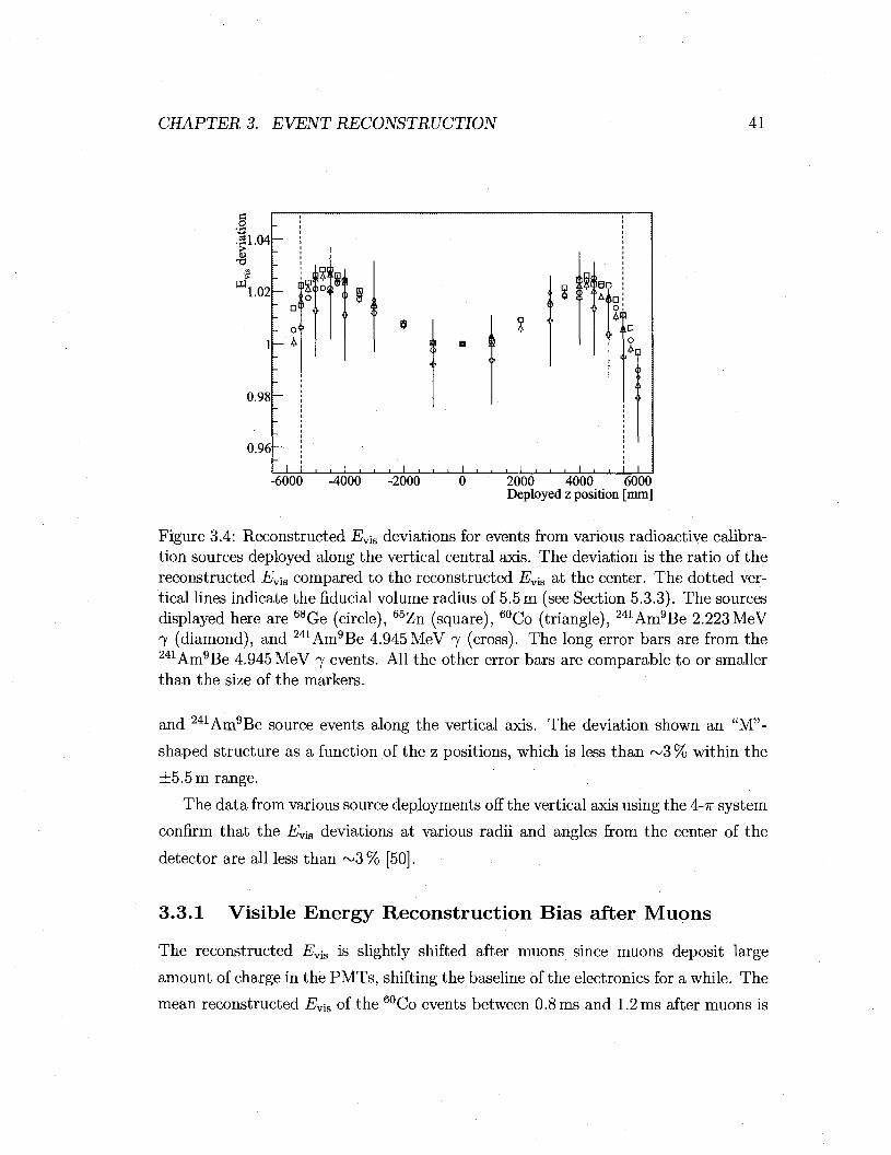
CHAPTER 3. EVENT RECONSTRUCTION 41
.31.04
I PJ 1.02
0.98
0.96
-6000 -4000
St n
Af 4°
o
-2000 _L
2000 4000 6000 Deployed z position [mm]
Figure 3.4: Reconstructed Evis deviations for events from various radioactive calibration sources deployed along the vertical central axis. The deviation is the ratio of the reconstructed Evis compared to the reconstructed Evis at the center. The dotted vertical lines indicate the fiducial volume radius of 5.5 m (see Section 5.3.3). The sources displayed here are 68Ge (circle), 65Zn (square), 60Co (triangle), 241Am9Be 2.223MeV 7 (diamond), and 241Am9Be 4.945MeV 7 (cross). The long error bars are from the 241Am9Be 4.945 MeV 7 events. All the other error bars are comparable to or smaller than the size of the markers.
and 241Am9Be source events along the vertical axis. The deviation shown an "M"-
shaped structure as a function of the z positions, which is less than ~ 3 % within the
±5.5 m range.
The data from various source deployments off the vertical axis using the 4-7T system
confirm that the Evi8 deviations at various radii and angles from the center of the
detector are all less than ~ 3 % [50].
3.3.1 Visible Energy Reconstruction Bias after Muons
The reconstructed Evis is slightly shifted after muons since muons deposit large
amount of charge in the PMTs, shifting the baseline of the electronics for a while. The
mean reconstructed EU. of the 60Co events between 0.8 ms and 1.2 ms after muons is

CHAPTER 3. EVENT RECONSTRUCTION 42
L . . . . . L L i - I — . . . .1 1 — J • • I ' ' • ' I • • ' i I i i i i
2.3 2.4 2.5 2.6 2.7 2.8 Reconstructed E^ [MeV]
Figure 3.5: Reconstructed EYis distribution for 60Co events chosen from 0.8 ms to 1.2 ms after muons (filled marker) and from 100 ms and 1 s after muons (open marker). A Gaussian is fitted to each of the distributions. The fit to the distribution with the filled markers (solid curve) yields a mean and sigma of 2.5427 ± 0.0064 MeV and 1.1866 ± 0.0063 MeV, respectively, and a x2/n.d.f. of 3.5/5. The fit to the histogram with the open markers (dotted curve) yields a mean and sigma of 2.52713± 0.00055 MeV and 0.12341 ± 0.00052 MeV, respectively, and a x*/n.d.f. of 41.9/47.
2.5427 ±0.0064 MeV while that of events more than 100 ms after muons is 2.52713 ±
0.00055 MeV, as shown in Figures 3.5, corresponding to a bias of 0.62 ± 0.25 %. The
reconstructed Evis is more biased if the events that follow muons in shorter times are
included. The mean reconstructed EV-1S of the 60Co events between 0.2 ms and 1.2 ms
after muons is 2.5452 ± 0.0042 MeV, corresponding to a bias of 0.72 ± 0.17%
3.4 Real Energy and Visible Energy
The real energy, Ereai, of a particle is defined to be the total kinetic energy of the
particle. For a positron, Eveai is its kinetic energy plus 1.022 MeV from the two 7s
produced in its annihilation with an electron. The light output from an event with
a given Ereai varies due to the effects of light quenching and Cherenkov radiation.
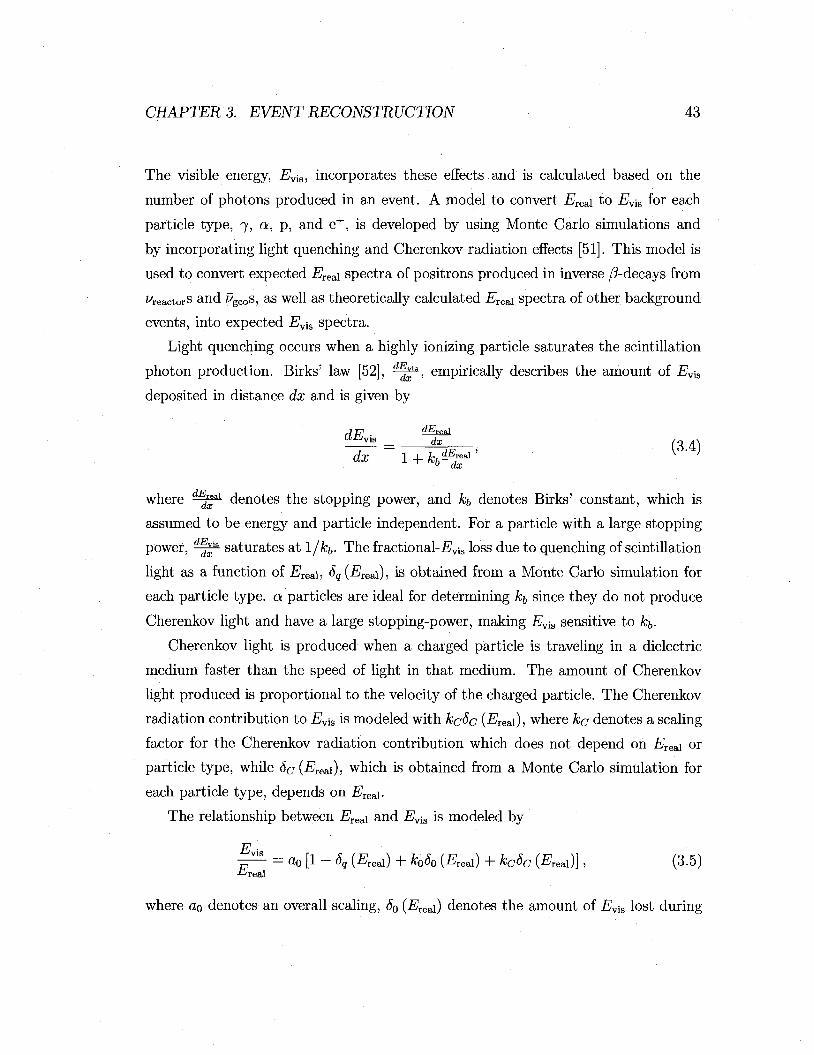
CHAPTER 3. EVENT RECONSTRUCTION 43
The visible energy, _Evig, incorporates these effects and is calculated based on the
number of photons produced in an event. A model to convert ETeai to Evis for each
particle type, 7, a, p, and e+ , is developed by using Monte Carlo simulations and
by incorporating light quenching and Cherenkov radiation effects [51]. This model is
used to convert expected lineal spectra of positrons produced in inverse /^-decays from
Reactors and ^geos, as well as theoretically calculated Eieax spectra of other background
events, into expected Ev[a spectra.
Light quenching occurs when a highly ionizing particle saturates the scintillation
photon production. Birks' law [52], ^ | ^ , empirically describes the amount of Evis
deposited in distance dx and is given by
^ = « L _ (3.4)
where E^x denotes the stopping power, and fc& denotes Birks' constant, which is
assumed to be energy and particle independent. For a particle with a large stopping
power, ^ ^ saturates at l/fc^. The fractional-Ev-i& loss due to quenching of scintillation
light as a function of EreSL\, 8q (ETeai), is obtained from a Monte Carlo simulation for
each particle type, a particles are ideal for determining kf, since they do not produce
Cherenkov light and have a large stopping-power, making Evis sensitive to fc&.
Cherenkov light is produced when a charged particle is traveling in a dielectric
medium faster than the speed of light in that medium. The amount of Cherenkov
light produced is proportional to the velocity of the charged particle. The Cherenkov
radiation contribution to EviS is modeled with kcSc (ETea,i), where kc denotes a scaling
factor for the Cherenkov radiation contribution which does not depend on Eiea\ or
particle type, while 6c(Eieai), which is obtained from a Monte Carlo simulation for
each particle type, depends on Eiea\.
The relationship between i?real and _Evis is modeled by
E •. a0 [1 - 5q (£ rea l) + k080 ( £ w ) + kc5c (£ r e a i)] , (3.5) E, real
where ao denotes an overall scaling, 80 (ETeax) denotes the amount of Evis lost during

CHAPTER 3. EVENT RECONSTRUCTION 44
Table 3.1: Energy calibration points. The central values are measurements at the center of the ID, and the errors include temporal and spatial variations. 68Ge and 60Co produce two 7s in an event, so the Ereai and the E^ for these events are divided by two. Unlike other calibration sources, 12C(n,7)13G, 214Po(0,4He)210Pb, and 212Po(0,4He)208Pb are distributed throughout the ID, and the central values are estimated by selecting only the events reconstructed near the center of the ID. The details of each calibration point measurement are described in Appendix E.
Calibration 203fjg
68Ge 65Zn 1H(n,7)2H (from 241Am9Be) 60Co 12C(n,7)13C 214Po(0,4He)210Pb 212Po(0,4He)208Pb
#real [MeV]
0.2791967 (1.022006)/2
1.115539 2.22457
(2.50572)/2 4.946431 7.68682 8.78486
Reconstructed Evis [MeV] 0.2400 ± 0.0055
(0.923 ± 0.013)/2 1.1031 ±0.0082 2.333 ± 0.025
(2.5057 ± 0.0093) /2 5.407 ± 0.064
0.6201 ± 0.0097 0.814 ±0.014
Table 3.2: Fitted energy parameters.
Parameter a0
h k0
kc
Best-fit value 1.061 ±0.024
0.00971 ± 0.00027gcm"2 MeV"1
0.84 ±0.14 0.43 ±0.11
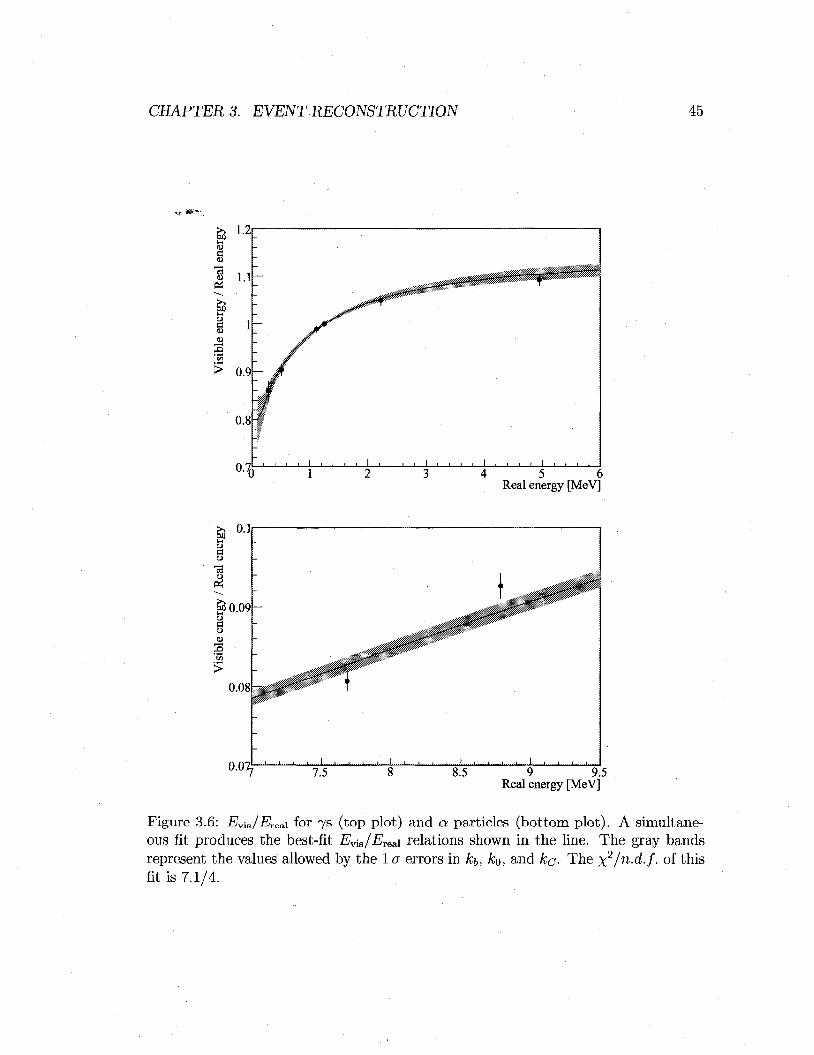
CHAPTER 3. EVENT RECONSTRUCTION 45
« d <u 73 u
g 3
5 6 Real energy [MeV]
s 73
£3 0.09 ID
a u
0.08ba
0 0 7 L_u__x 9.5
Real energy [MeV]
Figure 3.6: EviB/ETeai for 7s (top plot) and a particles (bottom plot). A simultaneous fit produces the best-fit Evis/Erea\ relations shown in the line. The gray bands represent the values allowed by the 1 a errors in kb, k0, and kc- The ^/n.d.f. of this fit is 7.1/4.
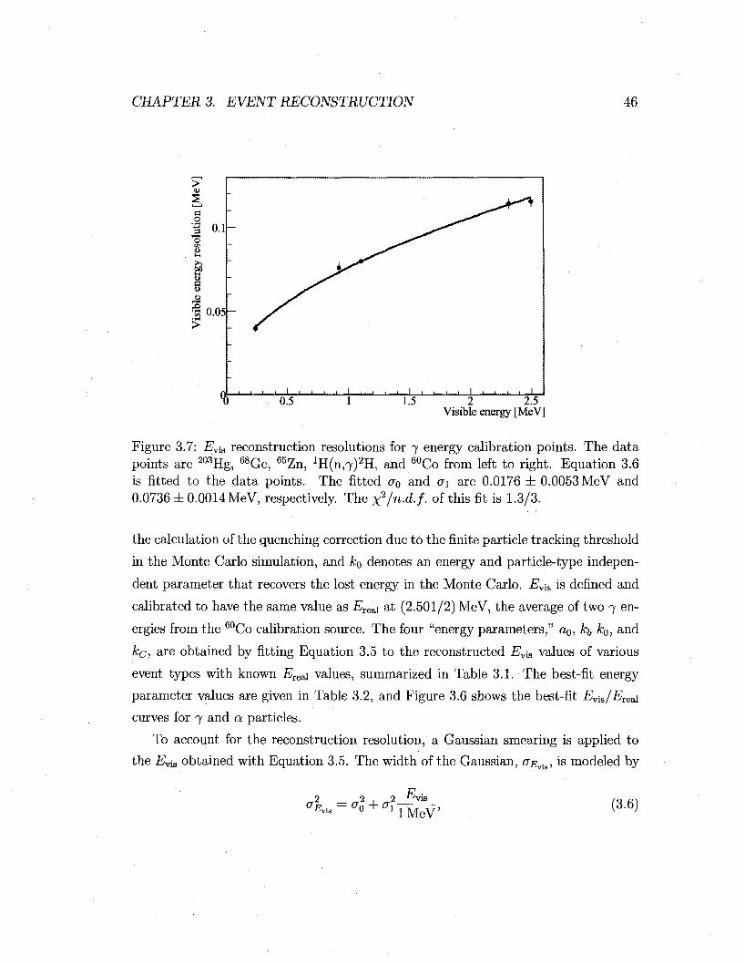
CHAPTER 3. EVENT RECONSTRUCTION 46
d o
'12 0.1
a u u 3 0.05
* 0.5 - J 1 1 l _
1.5 2 2.5 Visible energy [MeV]
Figure 3.7: EviS reconstruction resolutions for 7 energy calibration points. The data points are 203Hg, 68Ge, 65Zn, ^ ( n / y ) 2 ! ! , and 60Co from left to right. Equation 3.6 is fitted to the data points. The fitted a0 and o\ are 0.0176 ± 0.0053 MeV and 0.0736 ± 0.0014 MeV, respectively. The x 2 /n .d . / . of this fit is 1.3/3.
the calculation of the quenching correction due to the finite particle tracking threshold
in the Monte Carlo simulation, and k0 denotes an energy and particle-type indepen
dent parameter that recovers the lost energy in the Monte Carlo. Ev[s is defined and
calibrated to have the same value as ETeai at (2.501/2) MeV, the average of two 7 en
ergies from the 60Co calibration source. The four "energy parameters," a0, kb k0, and
kc, are obtained by fitting Equation 3.5 to the reconstructed E^ values of various
event types with known Ere&\ values, summarized in Table 3.1. The best-fit energy
parameter values are given in Table 3.2, and Figure 3.6 shows the best-fit Evis/Eieax
curves for 7 and a particles.
To account for the reconstruction resolution, a Gaussian smearing is applied to
the Evis obtained with Equation 3.5. The width of the Gaussian, OEV1B, is modeled by
2 F, • = er0 + er. x lMeV
(3.6)

CHAPTER 3. EVENT RECONSTRUCTION 47
where a0 accounts for the background photons, and o\ accounts for the statistical
fluctuations in the number of photons observed from the event of interest, GQ and o\
are estimated using the E^s reconstruction resolutions for 7 energy calibration points
from 203Hg, 68Ge, 65Zn, ^ ( n ^ H , and 60Co, as shown in Figure 3.7. The fitted <r0
and 0-1 are 0.0176 ± 0.0053 MeV and 0.0736 ± 0.0014 MeV, respectively.
3.5 Muon Track Reconstruction
Muons going through the detector produce a large amount of light by scintillation in
the LS and Cherenkov radiation in both the LS and the buffer oil. The muon track
reconstruction algorithm uses the arrival time distribution of the first photons that
hit each PMT. This algorithm uses the times of the pulses estimated by the LPA.
Cherenkov light is emitted at a constant angle, 6, with respect to the muon track,
forming the shape of a forward opening cone. Assuming that muons pass through the
detector at the same speed as that of light in vacuum, 6 is given by [53],
cos0 = i , (3.7) n
where n denotes the index of refraction in the LS and the buffer oil; although the LS
and the buffer oil have slightly different values of n's, for simplicity, a single value of
1.45 is used for both. Although the scintillation light is emitted isotropically, the first
scintillation photons to reach each PMT from a muon track are emitted at the same
angle as the Cherenkov light.
For a given muon track, the arrival time of the first photon, tfirst, that travels
directly from the track is estimated for each PMT. The probability for ith PMT
to have <ftfirstj, the difference between tfirst and the actual first photon arrival time,
-P(^firsti)) is modeled with a Gaussian function with an exponential tail and a 1%
contribution from uncorrelated pulses. The Gaussian function accounts for the jitter
in the direct light arrival times, and the exponential tail accounts for the indirect light
arrival times from the muon. The track is fitted by maximizing the likelihood (L^) for
the observed tfirst distribution. The muon track is rejected if the final x2 — —21ogL^

CHAPTER 3. EVENT RECONSTRUCTION 48
t) 0.2 0.4 0.6 0.8 1 1.2 1.4 1.6 (b [mm]/6500 mm)2
Figure 3.8: Distribution of reconstructed muon track impact parameter, b, versus NPEID- The vertical dotted line indicates the radius of the balloon, assumed to be spherical. The horizontal dotted line indicates the NPEID threshold for LS muon event tag (see Section 3.6).
is poor. The algorithm converges in finding ~99 % of muon tracks with reasonable
X2-
Figure 3.8 shows the distribution of NPEiD and reconstructed muon track impact
parameter, b, defined to be the shortest distance between the muon track and the
center of the ID. Muons with b < 6.5 m go through the LS producing both scintillation
and Cherenkov light, resulting in much larger NPEiD than muons with b > 6.5 m which
produce only Cherenkov light.
3.6 Event Tag and Multiplets
After events are reconstructed, each event is tagged according to the event type
selection cuts using variables, such as AfMaxID, NMaxoD (the sum of maximum iVoDtop>
NoDupper, NoDiower and iVoDbottom, see Section 2.3.3), NPEm, and RMSPEm (see
Section 3.1). An event can be tagged as multiple event types if it satisfies all the
•j5ii.r.: ::i :>;l;:.''i: s::r.v j , - -1 . : : i ' i • i \ r -,?• , I i i : : r ^ l ^ v - ' i - - .:. ;l i ' V :7> I -i:i.V: ;:i i t ft^-i
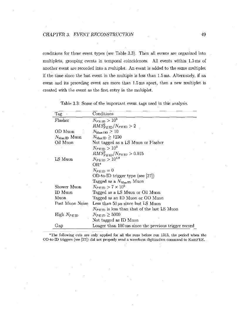
CHAPTER 3. EVENT RECONSTRUCTION 49
conditions for these event types (see Table 3.3). Then all events are organized into
multiplets, grouping events in temporal coincidences. All events within 1.5 ms of
another event are recorded into a multiplet. An event is added to the same multiplet
if the time since the last event in the multiple is less than 1.5 ms. Alternately, if an
event and its preceding event are more than 1.5 ms apart, then a new multiplet is
created with the event as the first entry in the multiplet.
Table 3.3: Some of the important event tags used in this analysis.
Tag Conditions
Flasher
OD Muon A W ID Muon Oil Muon
LS Muon
Shower Muon ID Muon Muon Post Muon Noise
High NPElD
Gap
N PEID >10 3
RMSPElD/NPElD > 2 AMaxOD > 10
iVMaxID > 1250
Not tagged as a LS Muon or Flasher NPEm > 103
RMSPEIJNPEW > 0.015 NPEm > 104-8
ORa
NPEID = 0 OD-to-ID trigger type (see [27]) Tagged as a AMaxiD Muon NPEID > 7 x 10⁵
Tagged as a LS Muon or Oil Muon Tagged as an ID Muon or OD Muon Less than 50 //s since last LS Muon NpEm is less than that of the last LS Muon NPEm > 5000 Not tagged as ID Muon Longer than 100 ms since the previous trigger record
aThe following cuts are only applied for all the runs before run 1313, the period when the OD-to-ID triggers (see [27]) did not properly send a waveform digitization command to KamFEE.

CHAPTER 3. EVENT RECONSTRUCTION 50

.* *
Chapter 4
Cosmogenic Spallation Products
Pions created by cosmic rays in the upper atmosphere decay into muons, which can
reach KamLAND. These muons, having very high energies, can activate the detector
material producing unstable nuclei by spallation processes while going through the
detector. These "spallation products" can represent important background events
to inverse /3-decay detection, but can also be useful to estimate various systematic
errors in this analysis due to their uniform distributions in the ID. If half-lives
are short, they are easily identifiable since they are produced in coincidence with
muons. The detector response for high energy events is studied using 12B /^-decays,
which have a relatively high endpoint energy. Spallation neutrons yield the mean
neutron capture time and the detector response at the neutron capture energy, both
of which are important since neutrons represent the tag for the inverse /?-decay. In
terms of background events, both high energy neutrons produced outside the detector
entering the LS and 9Li /^-decays produce spatially and temporally correlated events
that mimic inverse /3-decays and its subsequent neutron capture.
4.1 12B
Cosmic muons going through the detector produce radioactive 12B through reactions
with 12C in the LS [54]. 12B /^-decays into the stable 12C with a half-life of 20.20
± 0.02 ms and an endpoint energy of 13.4 MeV. These 12B /^-decays can serve as an
51
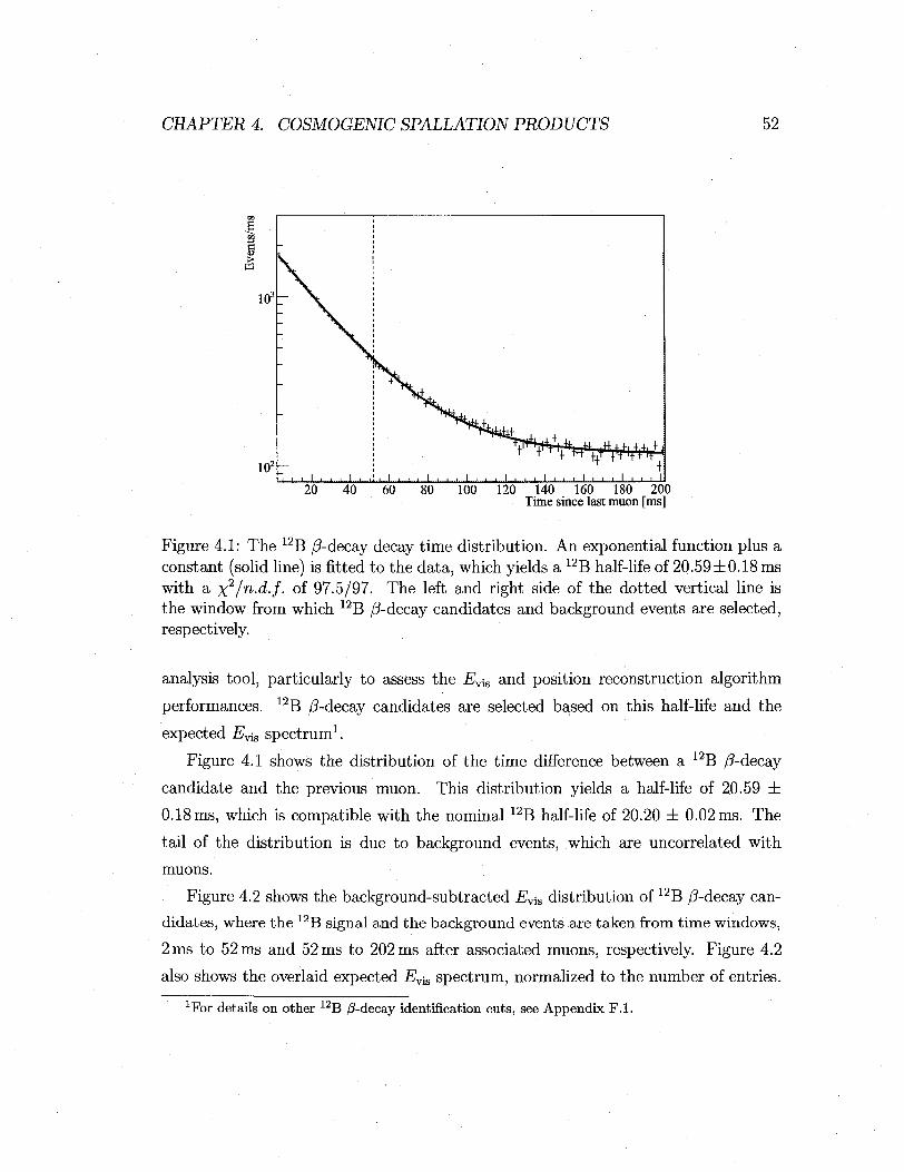
CHAPTER 4. COSMOGENIC SPALLATION PRODUCTS 52
»5
a
>
m
103
102
20 40 60 80 100 120 140 160 180 200 Time since last muon [ms]
Figure 4.1: The 12B /?-decay decay time distribution. An exponential function plus a constant (solid line) is fitted to the data, which yields a 12B half-life of 20.59 ±0.18 ms with a y^/n.d.f. of 97.5/97. The left and right side of the dotted vertical line is the window from which 12B /?-decay candidates and background events are selected, respectively.
analysis tool, particularly to assess the Evis and position reconstruction algorithm
performances. 12B /?-decay candidates are selected based on this half-life and the
expected EV1S spectrum1.
Figure 4.1 shows the distribution of the time difference between a 12B /?-decay
candidate and the previous muon. This distribution yields a half-life of 20.59 ±
0.18 ms, which is compatible with the nominal 12B half-life of 20.20 ± 0.02 ms. The
tail of the distribution is due to background events, which are uncorrelated with
muons.
Figure 4.2 shows the background-subtracted Evis distribution of 12B /?-decay can
didates, where the 12B signal and the background events are taken from time windows,
2 ms to 52 ms and 52 ms to 202 ms after associated muons, respectively. Figure 4.2
also shows the overlaid expected EV1S spectrum, normalized to the number of entries.
1For details on other 12B /3-decay identification cuts, see Appendix F.l.
J I I I 1 I I I I L L I I I I I I I I I I E I I I I I I I I I I I I I I I I—I 1 L
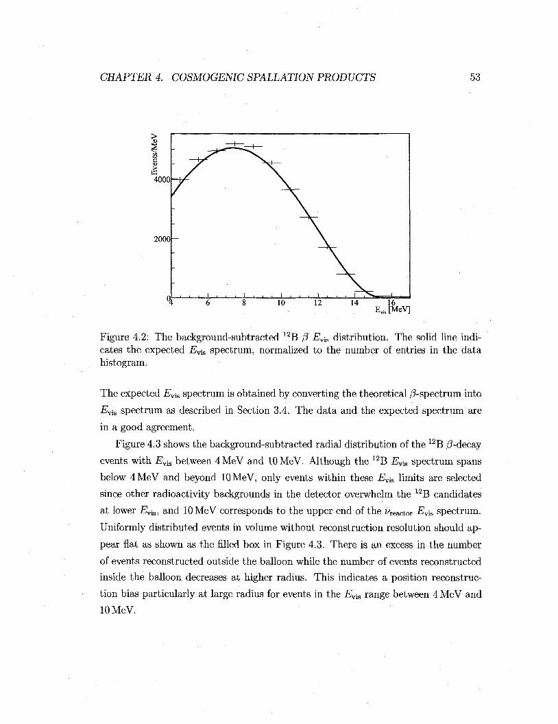
CHAPTER 4. COSMOGENIC SPALLATION PRODUCTS 53
£ 4000
2000H
16 EviJMeV]
Figure 4.2: The background-subtracted 12B /? Evis distribution. The solid line indicates the expected Evis spectrum, normalized to the number of entries in the data histogram.
The expected Ev{s spectrum is obtained by converting the theoretical /^-spectrum into
-Evis spectrum as described in Section 3.4. The data and the expected spectrum are
in a good agreement.
Figure 4.3 shows the background-subtracted radial distribution of the 12B /3-decay
events with Evis between 4 MeV and 10 MeV. Although the 12B Evis spectrum spans
below 4 MeV and beyond 10 MeV, only events within these Ev{s limits are selected
since other radioactivity backgrounds in the detector overwhelm the 12B candidates
at lower Evis, and 10 MeV corresponds to the upper end of the Reactor Evis spectrum.
Uniformly distributed events in volume without reconstruction resolution should ap
pear flat as shown as the filled box in Figure 4.3. There is an excess in the number
of events reconstructed outside the balloon while the number of events reconstructed
inside the balloon decreases at higher radius. This indicates a position reconstruc
tion bias particularly at large radius for events in the Evis range between 4 MeV and
10 MeV.
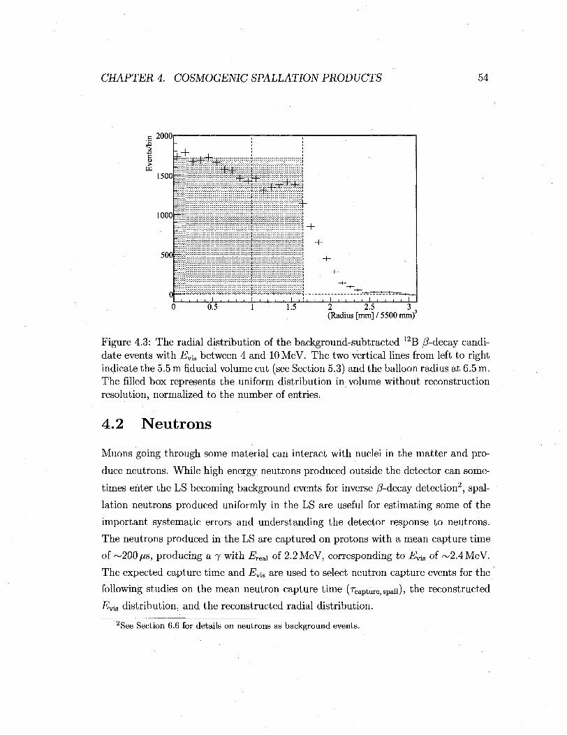
CHAPTER 4. COSMOGENIC SPALLATION PRODUCTS 54
.a 20001
> *nniii 1500
1000
500
0PS
0.5
m m. •K UHI ffl-
_L 1.5 2 2.5 3
(Radius [mm] / 5500 mm)
Figure 4.3: The radial distribution of the background-subtracted 12B /?-decay candidate events with £?vis between 4 and 10 MeV. The two vertical lines from left to right indicate the 5.5 m fiducial volume cut (see Section 5.3) and the balloon radius at 6.5 m. The filled box represents the uniform distribution in volume without reconstruction resolution, normalized to the number of entries.
4.2 Neutrons
Muons going through some material can interact with nuclei in the matter and pro
duce neutrons. While high energy neutrons produced outside the detector can some
times enter the LS becoming background events for inverse /3-decay detection2, spal
lation neutrons produced uniformly in the LS are useful for estimating some of the
important systematic errors and understanding the detector response to neutrons.
The neutrons produced in the LS are captured on protons with a mean capture time
of ~200/xs, producing a 7 with Ereai of 2.2 MeV, corresponding to EYis of ~2.4MeV.
The expected capture time and Ev{a are used to select neutron capture events for the
following studies on the mean neutron capture time (rcapture,spaii)) the reconstructed
Evis distribution, and the reconstructed radial distribution.
2See Section 6.6 for details on neutrons as background events.
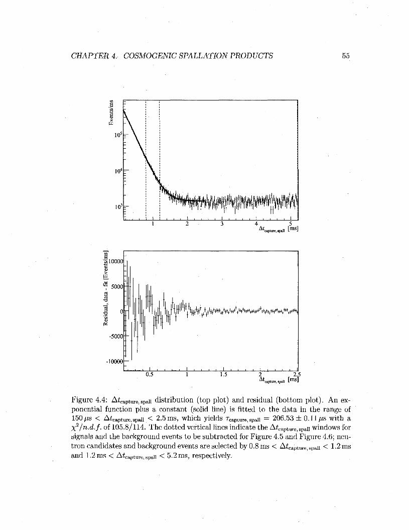
CHAPTER 4. COSMOGENIC SPALLATION PRODUCTS 55
##rtft/^ J__J I i I i L j _ L J I I 1 I L—I I L-
At capture, spall [ms]
"Si 0000 8 >
^ 5000
•3
-5000R-
-lOOOOH
oH
0.5
|tFp,\^^V%WM«^^^rtf ivH i
-' ' i '
1.5 -' ' ' ' 2 At.
_j 1 1 L_
capture, spall
2.5 [ms]
Figure 4.4: A£captUre,spall distribution (top plot) and residual (bottom plot). An exponential function plus a constant (solid line) is fitted to the data in the range of 150/is < Aicapture, spall < 2.5 ms, which yields rcapture, spall = 206.53 ± 0.11/xs with a X2/n.d.f. of 105.8/114. The dotted vertical lines indicate the Atcapturei spaU windows for signals and the background events to be subtracted for Figure 4.5 and Figure 4.6; neutron candidates and background events are selected by 0.8 ms < A£capture) span < 1.2 ms and 1.2 ms < AtCaPture, spall < 5.2 ms, respectively.

CHAPTER 4. COSMOGENIC SPALLATION PRODUCTS 56
T3 u o u o O
2.35H
(Radius [mm] / 5500 mm)
Figure 4.5: The corrected Evis for spallation neutrons and 241Am9Be neutrons. Each of the spallation neutron Evis points is background-subtracted, and then corrected for the reconstructed jE7ViS bias after muon, described in Section 3.3.1. Each of the 241Am9Be neutron EYis points is corrected for the source capsule shadowing, described in Appendix E.4.1. The black dots refer to the spallation neutrons with reconstructed positions in concentric spherical shells. The open circles refer to the spallation neutrons with reconstructed positions in 2 m-radius-cylinders along the vertical central axis of the detector. The open triangles refer to 241 Am9Be neutrons along the vertical central axis.
Figure 4.4 shows the distribution of the time difference between a spallation neu
tron candidate event3 and its previous muon, A£capture,Spaii- An exponential function
plus a constant are fitted to the data in the range of 150//s < Atcapturej span < 2.5 ms.
The lower fit limit of A£capture; spau = 150 /is is chosen to reduce the effect of recon
struction inefficiency and bias caused by large charge deposits of muons that affect
the detector for a while. This fit yields Tcapture, spall =
206.53 ± 0.11 /is. The constant
tail in t he distr ibution is produced by background events t ha t are uncorrelated wi th
muons.
The reconstructed neutron capture £"vis varies slightly depending on the position 3The details of the cuts to select spallaion neutrons for this study are discussed in Appendix F.2.1.
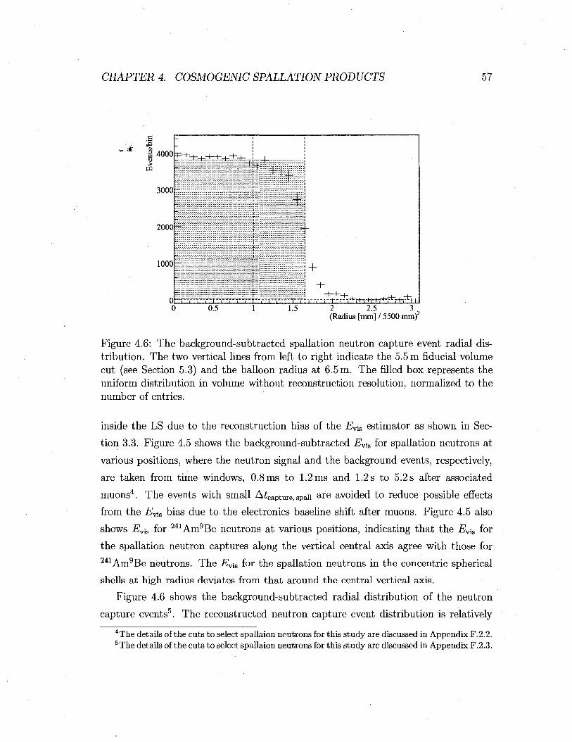
CHAPTER 4. COSMOGENIC SPALLATION PRODUCTS 57
| 4000 e >
3000
2000
1000
htiita
0.5
iBpiiiii
: Y > : : > ; : : : : : ^ : : : V > ^ ^
1 +
T T ? T ? ? ^ r f ? - t - - | " 7 - V r ty i- l -H ±Hd 1.5 2 2.5 3
(Radius [mm] / 5500 mm)
Figure 4.6: The background-subtracted spallation neutron capture event radial distribution. The two vertical lines from left to right indicate the 5.5 m fiducial volume cut (see Section 5.3) and the balloon radius at 6.5 m. The filled box represents the uniform distribution in volume without reconstruction resolution, normalized to the number of entries.
inside the LS due to the reconstruction bias of the Evis estimator as shown in Sec
tion 3.3. Figure 4.5 shows the background-subtracted Ev[s for spallation neutrons at
various positions, where the neutron signal and the background events, respectively,
are taken from time windows, 0.8 ms to 1.2 ms and 1.2 s to 5.2 s after associated
muons4. The events with small A£capture, span a r e avoided to reduce possible effects
from the EY-1S bias due to the electronics baseline shift after muons. Figure 4.5 also
shows .Evis for 241Am9Be neutrons at various positions, indicating that the Ev-ls for
the spallation neutron captures along the vertical central axis agree with those for 241Am9Be neutrons. The Evia for the spallation neutrons in the concentric spherical
shells at high radius deviates from that around the central vertical axis.
Figure 4.6 shows the background-subtracted radial distribution of the neutron
capture events5. The reconstructed neutron capture event distribution is relatively
4The details of the cuts to select spallaion neutrons for this study are discussed in Appendix F.2.2. 5The details of the cuts to select spallaion neutrons for this study are discussed in Appendix F.2.3.

CHAPTER 4. COSMOGENIC SPALLATION PRODUCTS 58
I 9|_i
13.6067
Figure 4.7: Decay schematic of 9Li [55].
flat within the 5.5 m radius from the center of the ID, and drops sharply at the balloon
radius of 6.5 m, indicating that the position reconstruction bias is small at neutron
capture Evia ~2.4MeV.
4.3 9Li
Cosmic muons going through the detector produce radioactive 9Li through reactions
with 12C in the LS [54]. 9Li /^-decays with a half-life of 178.3 ± 0.4 ms, sometimes
decaying to one of several excited states of 9Be, which then decays by neutron emission
as shown in Figure 4.7 [55]. The initial /?-decay and later neutron capture of the
emitted neutron produce two temporally and spatially correlated events, which can
mimic inverse /?-decay and its subsequent neutron capture. However, 9Li /?-decay
is easily identified by correlation with muons, forming triple coincidence events6:
muons, 9Li /^-decays, and neutron captures. An estimate of the expected number
of background event-pairs due to 9Li for Pe detection in this analysis is described in
Section 6.5. The Evis spectrum of the 9Li candidates can also be used to assess the
-Evis reconstruction performance. 6The 9Li candidates are selected by applying the Candidate Selection Cuts described in Sec
tion 5.3, except reversing the Shower/Misreconstructed Muon Cut and the Muon Cylinder Cut.
3% 11.81 _
1% 11.283 \
\v\
'.•4 16% 3.049
V30% 2.4294
9Be
3.0
8Be + n I i ,6654

CHAPTER 4. COSMOGENIC SPALLATION PRODUCTS 59
IS
w
103
102
0.2 0.4 0.6 0.8 1 1.2 1.4 1.6 1.8 2 Time since muons [s]
Figure 4.8: Time between events tagged as Shower Muons (see Section 3.6) and spallation 9Li /?-decay events. The thick line indicates the fit to an exponential function plus a constant, which yields the half-life of 190.2 ± 9.5 ms with a %2/n.d.f. of 25/27. The vertical dotted vertical lines indicate the time-since-muon windows for signals and the background events to be subtracted for Figure 4.9; 9Li /3-decay candidates and background events are selected from 2 ms to 0.5 s and 0.5 s to 1.5 s after associated muons, respectively.
Figure 4.8 shows the time difference between 9Li /3-decay candidates and events
tagged as Shower Muons7, muons which have a high light yield in the LS. Shower
Muons, compared to all the other categories of muons, produce most of 9Li in the LS.
The fitted half-life, 190.2 ± 9.5 ms is just outside of the 1 a error from the nominal 9Li
half-life of 178.3 ± 0.4 ms. Figure 4.9 shows the background-subtracted Ew-m spectrum
of the 9Li /?-decay candidates, where the 9Li /3-decay signal and the background events
are taken from time windows, 2 ms to 0.5 s and 0.5 s to 1.5 s after associated muons,
respectively. This distribution is overlaid with the expected Evm spectrum, normalized
to the number of entries. The expected Evis spectrum is obtained by converting the
theoretical /^-spectrum into EviS spectrum as described in Section 3.4. The data and
the expected spectrum are in reasonable agreement.
7See Section 3.6 for the definition of Shower Muon.
. i . i . i . . . i . . . i . . . i . . . i . : . i . . . i . i .

CHAPTER 4. COSMOGENIC SPALLATION PRODUCTS 60
Evis [MeV]
Figure 4.9: Background-subtracted Eyis spectrum of 9Li /?-decay events. The thick line indicates the expected spectrum normalized to the number of events in the histogram.
Chapter 5
Candidate Selection
The present analysis is based on data collected between April 2002 and April 2007.
After removing the calibration runs and the problematic run periods, the livetime is
calculated to be 1432.090 ± 0.072days (see Section 5.1). This analysis is based on a
spherical "fiducial volume" of radius 5.5 m in order to eliminate the outermost part
of the ID where backgrounds are higher, and event reconstruction algorithms are not
well-calibrated. The number of target protons within the fiducial volume is estimated
to be (4.59 ± 0.18) x 1031 (see Section 5.2).
The ue detection signature, prompt-delayed event-pairs produced by inverse f3-
decays and their subsequent neutron captures, is selected by applying a set of cuts,
described in Section 5.3, to reject backgrounds. The efficiencies of these cuts in
selecting inverse /3-decay are calculated in Sections 5.5 through 5.10.
5.1 Livetime
Extreme care has been taken to maximize the detector livetime1; the detector operates
around the clock taking data, except during the daily run change for a few minutes,
and occasional maintenance work, both of which add up to less than ~5 % of the
time. However, the detector sometimes operates under conditions not optimized for ue
Maximizing the detector livetime is important to increase the probability of detecting unpredictable events, such as a supernova explosion.
61
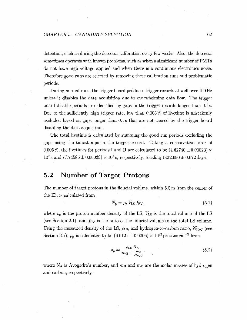
CHAPTER 5. CANDIDATE SELECTION 62
detection, such as during the detector calibration every few weeks. Also, the detector
sometimes operates with known problems, such as when a significant number of PMTs
do not have high voltage applied and when there is a continuous electronics noise.
Therefore good runs are selected by removing these calibration runs and problematic
periods.
During normal runs, the trigger board produces trigger records at well over 100 Hz
unless it disables the data acquisition due to overwhelming data flow. The trigger
board disable periods are identified by gaps in the trigger records longer than 0.1s.
Due to the sufficiently high trigger rate, less than 0.005 % of livetime is mistakenly
excluded based on gaps longer than 0.1s that are not caused by the trigger board
disabling the data acquisition.
The total livetime is calculated by summing the good run periods excluding the
gaps using the timestamps in the trigger record. Taking a conservative error of
0.005%, the livetimes for periods I and II are calculated to be (4.62740 ± 0.00023) x
107s and (7.74585 ±0.00039) x 107s, respectively, totaling 1432.090 ± 0.072 days.
5.2 Number of Target Protons
The number of target protons in the fiducial volume, within 5.5 m from the center of
the ID, is calculated from
WP = P P W F V , (5.1)
where pp is the proton number density of the LS, VLs is the total volume of the LS
(see Section 2.1), and / F V is the ratio of the fiducial volume to the total LS volume.
Using the measured density of the LS, PLS, and hydrogen-to-carbon ratio, JVH/C (see
Section 2.1), pp is calculated to be (6.6121 ±0.0066) x 1022 protons c m - 3 from
PV = , r~o , (5-2) mH + n H / C
where NA is Avogadro's number, and m^ and TUQ are the molar masses of hydrogen
and carbon, respectively.

CHAPTER 5. CANDIDATE SELECTION 63
. 0.65r
0.6h
0.55h
•iiiiiiiiiiiiiiii IMIIIIIIIIIIillllll I |
T ' r
1000 2000 3000 4000 -J L „ I..., I,..
5000 6000 Run number
Figure 5.1: / F V as a function of run number. The values represented by the circular and triangular markers are calculated with spallation 12B /?-decay and spallation neutron capture events, respectively. The gray bands indicate the statistical 1 a error range for /pys calculated from neutrons (top) and 12B (bottom). The thick solid horizontal line indicates the estimated central /FV value. The thick dotted horizontal line indicates the nominal / F V value if the fiducial radius is exactly 5500 mm without a reconstruction bias, and VLS — 1171 m3 (see Section 2.1).
/ F V is estimated using cosmogenic spallation 12B /^-decays and neutrons captures,
which are assumed to be uniformly produced in the LS by muons going through the
detector, /py is given by the number of events whose reconstructed radius is within
5500 mm compared to the total number of events. The estimated / F V using 12B (3-
decays with 4 MeV < Evis < 10 MeV is 0.5735 ± 0.0035, and the estimated / F V using
neutron captures is 0.6129 ± 0.0043. Figure 5.1 shows the / F V estimated with 12B
and neutrons function of run number.
The difference between /py calculated with 12B /^-decays and neutron captures is
not completely understood. It is possible that such difference is due to the dependence
of the position reconstruction algorithm on EY-ls. Figure 5.2 shows /py as a function of 12B (3 -Evis, which is relatively stable between 4 MeV and 10 MeV. However, it appears
that the position reconstruction performance changes between ~2 MeV and ^ 5 MeV
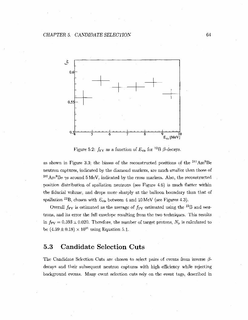
CHAPTER 5. CANDIDATE SELECTION 64
J I I 1 I I I I I I L_J I I I 1 1 I I 1 1 1 i I 1 1 1 1 1 1
5 6 7 8 9 10 Evis [MeV]
Figure 5.2: /Fv as a function of EVjS for 12B /^-decays.
as shown in Figure 3.3; the biases of the reconstructed positions of the 241Am9Be
neutron captures, indicated by the diamond markers, are much smaller than those of 241Am9Be 7s around 5 MeV, indicated by the cross markers. Also, the reconstructed
position distribution of spallation neutrons (see Figure 4.6) is much flatter within
the fiducial volume, and drops more sharply at the balloon boundary than that of
spallation 12B, chosen with Evis between 4 and 10 MeV (see Figures 4.3).
Overall /FV is estimated as the average of /F V estimated using the 12B and neu
trons, and its error the full envelope resulting from the two techniques. This results
in /Fv = 0.593 ± 0.020. Therefore, the number of target protons, Np is calculated to
be (4.59 ± 0.18) x 1031 using Equation 5.1.
5.3 Candidate Selection Cuts
The Candidate Selection Cuts are chosen to select pairs of events from inverse (3-
decays and their subsequent neutron captures with high efficiency while rejecting
background events. Many event selection cuts rely on the event tags, described in
0.6
0.55
CHAPTER 5. CANDIDATE SELECTION 65
Section 3.6.
5.3.1 Basic Good Event Cuts
The following cuts are applied to ensure good data quality within the selected runs.
• - MaxiD Cut: Only events with iVjyiaxiD greater than or equal to 200 for period I
and 180 for period II2 are considered to avoid events with lower A MaxiD that
are occasionally acquired during normal runs with special trigger types and
unknown triggering efficiencies. The iVMaxID threshold efficiency is calculated
in Section 5.5.
• Multiplet Cut: If a multiplet, described in Section 3.6, has more than 9 events,
all the events in the multiplet are removed to eliminate a noisy period. Since the
average event rate is a few tens of Hz, this process removes negligible number
of good events.
• Reconstruction Status Cut: Events must have valid position and Evis recon
struction statuses. The reconstruction efficiency is estimated in Section 5.6.
5.3.2 Cosmogenic Spallation Cuts
The following cuts are applied to avoid muons and their spallation products that can
mimic inverse /^-decays and their subsequent neutron captures, such as short-lived
neutrons (see Section 4.2) and long-lived 9Li, produced along the paths of muons (see
Section 4.3). The efficiency due to these cuts is estimated in Section 5.7.
• Shower/Misreconstructed Muon Cut: The full detector volume is vetoed for 2 s
after an event tagged as a Shower Muon or an ID Muon on which the muon
track reconstruction algorithm failed since such an event can produce various
long-lived spallation products, such as 9Li. 2These periods are defined by when the thermometers were removed (see Section 2.1). However,
this period boundary is only 6 days after the Nm trigger threshold was lowered from 200 to 180.

CHAPTER 5. CANDIDATE SELECTION 66
• Muon Cut: The full detector volume is vetoed for 2 ms after an event tagged
as a Muon to avoid noise caused by the electronics and PMTs after muons and
short-lived spallation products, such as neutrons.
• Muon Cylinder Cut: The volume in a cylinder of radius 3 m from the muon
track is vetoed for 2 s after an ID Muon with a valid reconstructed muon track
to avoid long-lived spallation products such as 9Li along the muon track. This
cut is applied only to the prompt candidate events described in Section 5.3.3.
• High NPEID Event Cut: The full detector volume is vetoed for 2 ms after an
event tagged as a High NPEID- Undetected muons outside the detector can
produce high energy neutrons that reach the LS, and the thermalization of
these high energy neutrons in the LS can cause High A/pEID events. Such high
energy neutrons can also create secondary neutrons, and the captures of these
neutrons can mimic inverse /^-decays and their subsequent neutron captures.
The High NPEID Event Cut is designed to reduce these background events. See
Section 6.6 for more details on spallation neutrons as background events.
• Gap Cut: Muons could have passed through the detector producing long-lived
spallation products while the trigger board was disabled. Therefore the full
detector volume is vetoed for 2 s after an event tagged as a Gap, which identifies
periods when the trigger board was disabled.
5.3.3 Coincidence Selection Cuts
The following cuts are applied to select inverse /^-decays and their subsequent neutron
captures with high efficiency, using their temporal and spatial coincidence signals, and
the narrow Ev[s distribution of the neutron capture 7.
• AR Cut: Ai? < 1600 mm, where AJ? denotes the distance between the prompt
and delayed events. Section 5.8 discusses the efficiency of this cut.
• At Cut: 0.5/xs < At < 1000/xs, where At denotes the time between the prompt
and delayed events. Section 5.9 discusses the efficiency of this cut.
CHAPTER 5. CANDIDATE SELECTION 67
• Ep Cut: 0.9MeV < Ep < 15MeV for period I.and 0.8MeV < Ep < 15MeV
for period II, where Ep denotes the Evis of the prompt events. The detector
iViD threshold was lowered in period II enabling the analysis Ew-m threshold
to be lowered in order to increase the efficiency. Although the expected E^
spectrum for PreactorS spans only up to ~10 MeV, events with Evia up to 15 MeV
are included to gain a better constraint on high energy background events (see
Sections 6.6 and 6.7). The efficiency of this cut is calculated during the fit (see
Chapter 7) since the energy parameters (see Section 3.4) are simultaneously
fitted, which changes the expected Ep spectral shape.
• Ed Cut: 2.04 MeV < Ed < 2.76 MeV, where Ed denotes the Evis of the delayed
events. Most of the neutrons produced in inverse /?-decay are captured by
protons in the LS creating 2.2 MeV 7s, which corresponds to Evis of ^2.4 MeV.
Section 5.10 discusses the efficiency of this cut.
• - average Cut: To avoid the sections of the detector where the position recon
struction bias is large, and to avoid the large number of background events that
are produced at the balloon surface near 6.5 m, the fiducial volume is defined
to be within the 5.5 m from the center of the ID. This cut is applied on the
average radius of the prompt-delayed event-pair, i?average-
• High Candidate Multiplet Cut: The prompt and delayed candidate event-pair is
isolated from other pairs. For example, if three events form two or three pairs,
all of them are thrown away. The probability of two events from an inverse j3-
decay and its subsequent neutron capture being coincident with another event
is negligible, and such multiple coincidence events are likely caused by thermal-
ization and captures of high energy spallation neutrons and those of secondary
neutrons that they produce (see Sections 6.6).
5.4 Simulated Delayed Event Distribution
The fiducial volume cut, -Raverage < 5.5 m, is applied to the radius of the average
positions of the prompt and delayed event-pairs to ensure constant detection efficiency
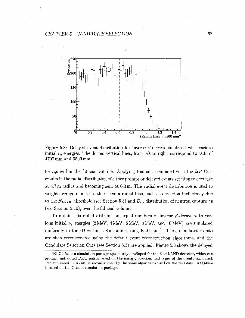
CHAPTER 5. CANDIDATE SELECTION 68
(Radius [mm] / 5500 mm)
Figure 5.3: Delayed event distribution for inverse /^-decays simulated with various initial Pe energies. The dotted vertical lines, from left to right, correspond to radii of 4700 mm and 5500 mm.
for Pes within the fiducial volume. Applying this cut, combined with the AR Cut,
results in the radial distribution of either prompt or delayed events starting to decrease
at 4.7 m radius and becoming zero at 6.3 m. This radial event distribution is used to
weight-average quantities that have a radial bias, such as detection inefficiency due
to the NuaxiD threshold (see Section 5.5) and Evis distribution of neutron capture 7s
(see Section 5.10), over the fiducial volume.
To obtain this radial distribution, equal numbers of inverse /^-decays with var
ious initial ue energies (2 MeV, 4 MeV, 6 MeV, 8 MeV, and 10 MeV) are simulated
uniformly in the ID within a 8 m radius using KLG4sim3. These simulated events
are then reconstructed using the default event reconstruction algorithms, and the
Candidate Selection Cuts (see Section 5.3) are applied. Figure 5.3 shows the delayed
3KLG4sim is a simulation package specifically developed for the KamLAND detector, which can produce individual PMT pulses based on the energy, position, and types of the events simulated. The simulated data can be reconstructed by the same algorithms used on the real data. KLG4sim is based on the Geant4 simulation package.
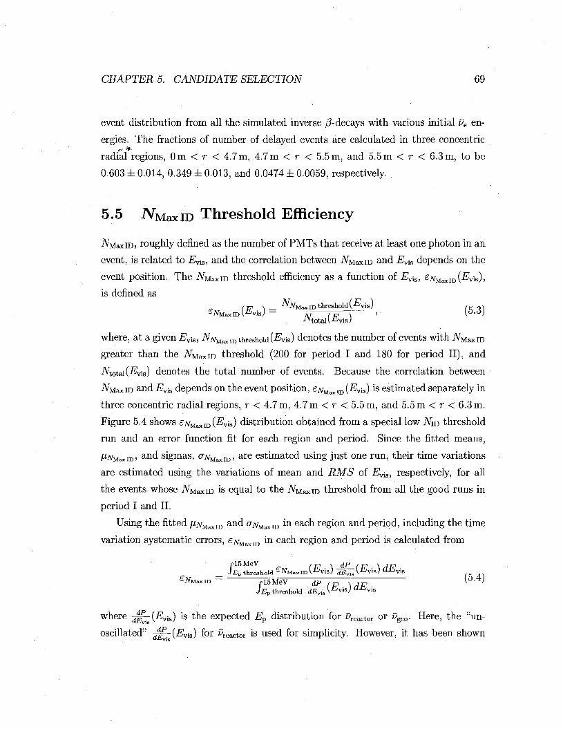
CHAPTER 5. CANDIDATE SELECTION 69
/ p \ _ i*iVMaxIDthresholdV-'- /vis,; (K Q N
event distribution from all the simulated inverse /^-decays with various initial i/e en
ergies. The fractions of number of delayed events are calculated in three concentric
radial regions, Om < r < 4.7m, 4.7m < r < 5.5m, and 5.5m < r < 6.3m, to be
0.603 ± 0.014, 0.349 ± 0.013, and 0.0474 ± 0.0059, respectively.
5.5 ATMaxID Threshold Efficiency
A MaxiD) roughly defined as the number of PMTs that receive at least one photon in an
event, is related to EV-1S, and the correlation between iVMaxiD and EviS depends on the
event position. The iVMaxiD threshold efficiency as a function of EV-1S, eNu^mi^is),
is denned as
-^MaxlD threshold V-^vis )
Ntotal(-Evis)
where, at a given Evis, NNMaxlothreshoXd(Evis) denotes the number of events with iVMaxiD
greater than the iVMaxiD threshold (200 for period I and 180 for period II), and
-Ntotai(-Evis) denotes the total number of events. Because the correlation between
-A MaxiD and Evis depends on the event position, £jvMaxiD(-Evis) is estimated separately in
three concentric radial regions, r < 4.7 m, 4.7 m < r < 5.5 m, and 5.5 m < r < 6.3 m.
Figure 5.4 shows £jvMaxID(.Evis) distribution obtained from a special low iVm threshold
run and an error function fit for each region and period. Since the fitted means,
A*/VMaxm> and sigmas, crjvMaxID, are estimated using just one run, their time variations
are estimated using the variations of mean and RMS of Evia, respectively, for all
the events whose iV~MaxID is equal to the iVMaxID threshold from all the good runs in
period I and II.
Using the fitted AtjvMaxID and erjvMaxID in each region and period, including the time
variation systematic errors, £7vMaxID in each region and period is calculated from
— p t h r o s h o l d £ J V M " - I D V-^V'SJ dEvla V-^visJ dEvm £JVMaxiD - r l5MeV dP (p \ 7^ ^ '
JEp threshold dEviB l -^visj " -^vis
where ^-(E^) is the expected Ep distribution for factor o r geo- Here, the "un-
oscillated" -^-{Ev-ls) for ureactor is used for simplicity. However, it has been shown

CHAPTER 5. CANDIDATE SELECTION 70
0.7 0.75 0.1 0.85 0.9 0.95 1 1.05 1.1 1.15 Reconstructed E ^ [MeV]
0.5
0.6 0.65 0.7
^ Max ID threshold '•**'
' 0.75 0.8 0.85 0.9 0.95 1 1.05
Reconstructed Evjs [MeV]
Figure 5.4: £NMaxiD(^vis) in three concentric radial regions in the detector from run 3888, which has a low -/VID threshold of 35. T h e top and bo t t om plots are for A^v[axID
thresholds of 200 and 180, respectively. The triangle, circle, and square markers are for data obtained from r < 4.7 m, 4.7 m < r < 5.5 m, and 5.5 m < r < 6.3 m, respectively. The solid curves are the fits to error functions. The dotted vertical line indicates the analysis j vis threshold of 0.9 MeV for period I and 0.8 MeV for period II.
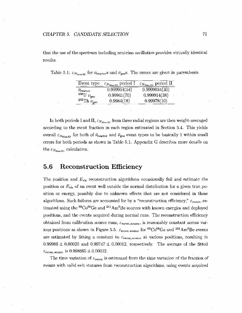
CHAPTER 5. CANDIDATE SELECTION 71
that the use of the spectrum including neutrino oscillation provides virtually identical
results.
Table 5.1: £jvMaxID for factors and ugeos. The errors are given in parenthesis.
Event type £jyMaxID
period I £jyMaxID period II factor 0.999954(54) 0.9999934(30) 238UPgeo 0.99941(70) 0.999914(38) 232Th ugeo 0.9984(18) 0.99978(10)
In both periods I and II, £jvMaxID from three radial regions are then weight-averaged
according to the event fraction in each region estimated in Section 5.4. This yields
overall £NMaxm fc>r both of Preactor a n d vgeo event types to be basically 1 within small
errors for both periods as shown in Table 5.1. Appendix G describes more details on
the £jvMaxro calculation.
5.6 Reconstruction Efficiency
The position and EviS reconstruction algorithms occasionally fail and estimate the
position or Evis of an event well outside the normal distribution for a given true po
sition or energy, possibly due to unknown effects that are not considered in these
algorithms. Such failures are accounted for by a "reconstruction efficiency," erecon, es
timated using the 60Co68Ge and 241Am9Be sources with known energies and deployed
positions, and the events acquired during normal runs. The reconstruction efficiency
obtained from calibration source runs, ereCon,source; is reasonably constant across var
ious positions as shown in Figure 5.5. erecon, source for 60Co68Ge and 241Am9Be events
are estimated by fitting a constant to £reCon, source at various positions, resulting in
0.99986 ± 0.00020 and 0.99747 ± 0.00012, respectively. The average of the fitted
£recon,source iS 0 .998665 ± 0 . 0 0 0 1 2 .
The time variation of £reCon is estimated from the time variation of the fraction of
events with valid exit statuses from reconstruction algorithms, using events acquired
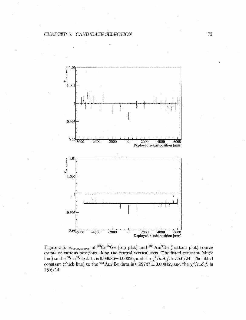
CHAPTER 5. CANDIDATE SELECTION 72
s l.Oli
J 1.005h
0.995
0.99'
M. ]—+
-J I L. J i i i I i i i I i i i L
6000 -4000 -2000 0 2000 4000 6000 Deployed z-axis position [mm]
1.01
1.005
0.995H
0.991
-6000 -4000 -2000 0 2000 4000 6000 Deployed z-axis position [mm]
Figure 5.5: erecon,source of 60Co68Ge (top plot) and Am Be (bottom plot) source events at various positions along the central vertical axis. The fitted constant (thick line) to the 60Co68Ge data is 0.99986±0.00020, and the x2/n.d.f. is 35.0/24. The fitted constant (thick line) to the 241Am9Be data is 0.99747 ± 0.00012, and the jn.d.f. is 18.6/14.
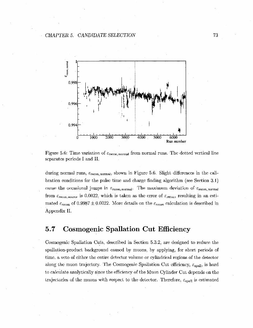
CHAPTER 5. CANDIDATE SELECTION 73
0.998
0.996
0.994
I.V M%%H r1 '
W™
-1 i u t-.,-L -J I 1 I I I L.
0 1000 2000 3000 4000 5000 6000 Run number
Figure 5.6: Time variation of £recon, normal from normal runs. The dotted vertical line separates periods I and II.
during normal runs, erecon,normal, shown in Figure 5.6. Slight differences in the cali
bration conditions for the pulse time and charge finding algorithm (see Section 3.1)
cause the occasional jumps in ereCon,normal- The maximum deviation of £recon, normal
from £recon, source is 0.0022, which is taken as the error of £reCon, resulting in an esti
mated £reCon of 0.9987 ± 0.0022. More details on the erecoii calculation is described in
Appendix H.
5.7 Cosmogenic Spallation Cut Efficiency
Cosmogenic Spallation Cuts, described in Section 5.3.2, are designed to reduce the
spallation-product background caused by muons, by applying, for short periods of
time, a veto of either the entire detector volume or cylindrical regions of the detector
along the muon trajectory. The Cosmogenic Spallation Cut efficiency, espaii, is hard
to calculate analytically since the efficiency of the Muon Cylinder Cut depends on the
trajectories of the muons with respect to the detector. Therefore, espau is estimated
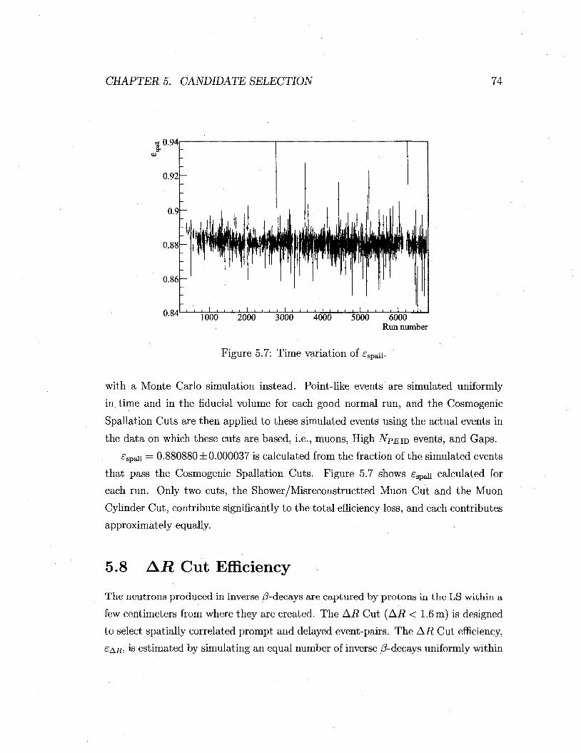
CHAPTER 5. CANDIDATE SELECTION 74
= 0.94 CO
0.92
0.9
0.88
0.86
1000 2000 3000 4000 5000 6000 Run number
Figure 5.7: Time variation of eSpaii-
with a Monte Carlo simulation instead. Point-like events are simulated uniformly
in, time and in the fiducial volume for each good normal run, and the Cosmogenic
Spallation Cuts are then applied to these simulated events using the actual events in
the data on which these cuts are based, i.e., muons, High NPEm events, and Gaps.
£Spaii = 0.880880 ±0.000037 is calculated from the fraction of the simulated events
that pass the Cosmogenic Spallation Cuts. Figure 5.7 shows espau calculated for
each run. Only two cuts, the Shower/Misreconstructted Muon Cut and the Muon
Cylinder Cut, contribute significantly to the total efficiency loss, and each contributes
approximately equally.
5.8 AR Cut Efficiency
The neutrons produced in inverse /?-decays are captured by protons in the LS within a
few centimeters from where they are created. The AR Cut (AR < 1.6 m) is designed
to select spatially correlated prompt and delayed event-pairs. The AR Cut efficiency,
£AR-I is estimated by simulating an equal number of inverse /?-decays uniformly within
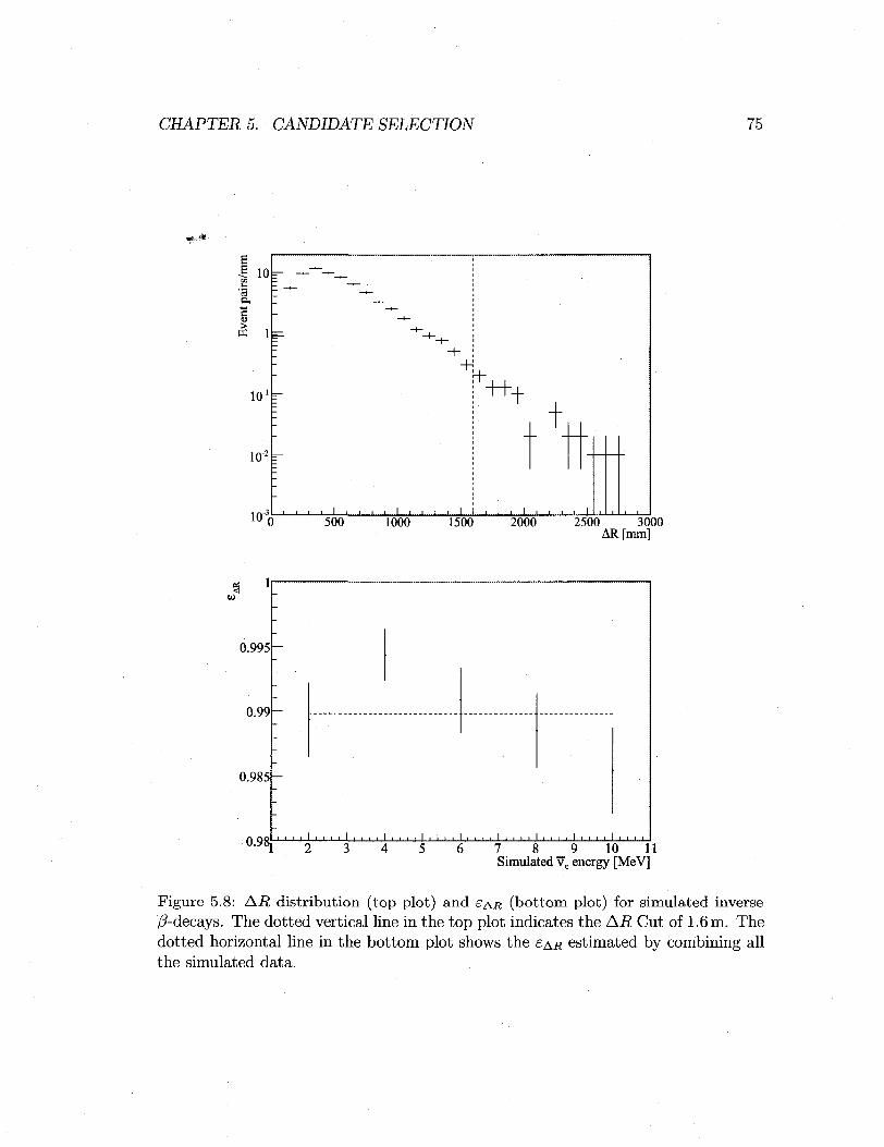
CHAPTER 5. CANDIDATE SELECTION 75
* • • «
3 i
101
i < r -
10
: -—
=p
-
—
"
-—
~*~-t-
+
X t
500 1000 1500 2000 2500 3000 AR[mm]
0.995H
0.99
0.985H
0.98J-1-1-1
2 3 4 5 6 7 8 _ 9 10 11 Simulated ve energy [MeV]
Figure 5.8: AR distr ibution (top plot) and e&.R (bo t tom plot) for simulated inverse /3-decays. The dotted vertical line in the top plot indicates the AR Cut of 1.6 m. The dotted horizontal line in the bottom plot shows the EAR estimated by combining all the simulated data.

CHAPTER 5. CANDIDATE SELECTION 76
E 10 '3
1 W
1
10'
10"2
1U 0 500 1000 1500 2000 2500 3000 3500 4000 AR [mm]
Figure 5.9: AR distributions of actual (dots with error bars) and simulated (solid line) 241Am9Be source events. The distribution from actual data is normalized to the number of entries for the simulated data. The dotted vertical line indicates the AR Cut of 1.6 m.
the ID from ues with energies at 2MeV, 4MeV, 6MeV, 8MeV, and lOMeV using
KLG4sim. The simulated data are processed using the default event reconstruction
algorithms, and AR is calculated from the simulated prompt-delayed event-pairs that
pass the Candidate Selection Cuts except the AR Cut (see Section 5.3.3).
The top plot in Figure 5.8 shows the resulting AR distribution; 98.87% of the
pairs in this distribution pass the AR Cut. This efficiency, e&R, depends slightly
on the energy of the simulated Pes, as shown in the bottom plot in Figure 5.8. The
maximum dispersion of 0.0057, shown in this figure, is taken as the error on EAR-
Possible differences between the simulation and real data are addressed by com
paring the AR distribution from 241Am9Be data simulated by KLG4sim to that
from actual 241Am9Be calibration data. The 241Am9Be source produces coincidence
events where the first events are either the thermalization of the neutrons alone or
that together with a 7, and the second events are the neutron captures on protons
in the LS. The AR distributions from actual and simulated 241Am9Be data are
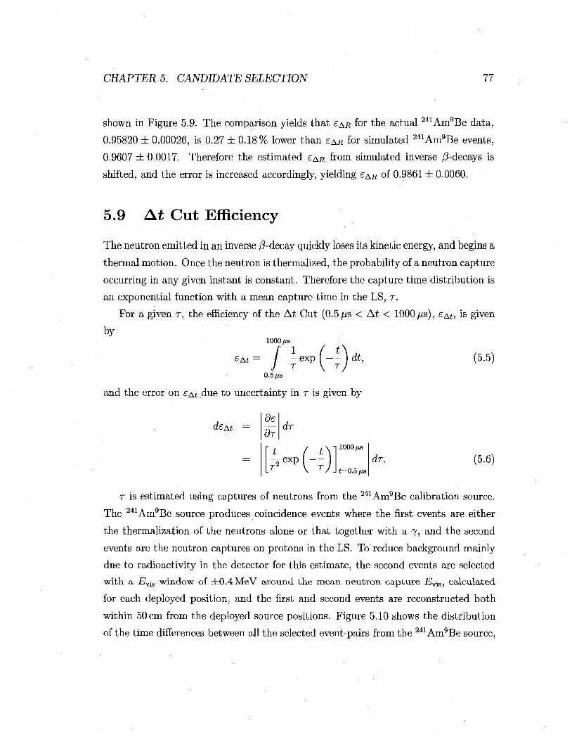
CHAPTER 5. CANDIDATE SELECTION 77
shown in Figure 5.9. The comparison yields that EAR for the actual 241Am9Be data,
0.95820 ± 0.00026, is 0.27 ± 0.18% lower than eAR for simulated 241Am9Be events,
0.9607 ± 0.0017. Therefore the estimated EAR from simulated inverse /3-decays is
shifted, and the error is increased accordingly, yielding CAR of 0.9861 ± 0.0060.
5.9 At Cut Efficiency
The neutron emitted in an inverse /?-decay quickly loses its kinetic energy, and begins a
thermal motion. Once the neutron is thermalized, the probability of a neutron capture
occurring in any given instant is constant. Therefore the capture time distribution is
an exponential function with a mean capture time in the LS, r.
For a given r , the efficiency of the At Cut (0.5//s < At < 1000/xs), e^t, is given
by 1000 fj,s
£te
0.5/JS
dt, (5.5)
and the error on e&t due to uncertainty in r is given by
dsAt = de dr
dr
' t i
J2 exp^ ' *M >-)]
1000 / «
t=0.5/Lts
dr. (5.6)
r is estimated using captures of neutrons from the 241Am9Be calibration source.
The 241Am9Be source produces coincidence events where the first events are either
the thermalization of the neutrons alone or that together with a 7, and the second
events are the neutron captures on protons in the LS. To reduce background mainly
due to radioactivity in the detector for this estimate, the second events are selected
with a i7VjS window of ± 0 . 4 MeV around t h e mean neut ron cap ture £7vis, calculated
for each deployed position, and the first and second events are reconstructed both
within 50 cm from the deployed source positions. Figure 5.10 shows the distribution
of the time differences between all the selected event-pairs from the 241Am9Be source,

CHAPTER 5. CANDIDATE SELECTION 78
200 400 600 800 1000 1200 1400 AtAmBe [n S]
> 0.02:
-0.02
t,
*W> A «i
200 400 600 800 1000 1200 At,
1400 xlOJ
,[ns]
Figure 5.10: AtAmBe distribution (top plot) and residual distribution (bottom plot). The solid curve in the top plot is the fit to an exponential function plus a constant from AtAmBe of 30 //s to 1.5 ms. The fitted r is 205.44 ± 0.60 fj,s, and the x2/ra.<f./. of this fit is 105.6/97.

CHAPTER 5. CANDIDATE SELECTION 79
215
214
213
212
-, , , ,
<> i i
i
, , , , ! . , , . , , , , ! , , , ,
(i
( 1
, . , . ! . . . , i ,
i
2.5 3.5 4.5 55 6 6.5 7 r 7.5 Log (neutron energy [eV])
Figure 5.11: r estimated from bare neutrons (filled markers) simulated at various initial neutron energies and simulated 241Am9Be neutrons (open marker). The horizontal error bar for the simulated 241Am9Be neutrons indicates their neutron energy range. The thick horizontal line is the weighted average of r from the bare neutrons at various energies, 213.47/xs.
A AmBe- An exponential function plus a constant is fitted to the A AmBe distribution
in the range of 30/xs < AiAmBe < 1.5 ms, where the lower limit is chosen to avoid the
period when ATWDs are more likely to be busy recording the first events. The fit
yields r = 205.44 ± 0.60/xs.
r obtained with neutrons produced by the 241Am9Be source may slightly differ
from that obtained with isolated neutrons because of neutron captures in the ma
terials composing the 241Am9Be source and its deployment equipment. This possi
ble bias is assessed with KLG4sim by simulating monoenergetic "bare" neutrons at
various energies (IkeV, 0.01 MeV, 0.1 MeV, 1 MeV, 3MeV, 5MeV, and 7MeV) and 241Am9Be neutrons with the deployment equipment, and comparing the resulting
neutron capture times. Although the neutrons from inverse /?-decays have energies
between ~lkeV and ~0.1MeV, bare neutrons with higher energies are simulated to
CHAPTER 5. CANDIDATE SELECTION 80
confirm that the capture time is consistent for higher neutron energies that are rele
vant for background events for inverse /?-decay detection (see Chapter 6). Figure 5.11
shows the resulting r for these simulated neutrons; the estimated r for neutrons at
various energies are consistent. A weighted average of r is calculated to be 213.47//s,
and the maximum r deviation of 0.39 /xs from the weighted average is taken as its
error.
The simulated 241Am9Be neutrons yield r of 212.96 ± 0.65/xs. This is slightly
lower than 213.47 ± 0.39/is from simulated bare neutrons. Approximately 1% of
the simulated 241Am9Be neutrons are captured on the source containment capsule,
which contains mostly iron. Iron has an approximately ten times larger cross-section
for neutron capture than protons, so the 241Am9Be neutrons are expected to have a
slightly shorter mean capture time than bare neutrons, r estimated from simulated
neutrons are significantly higher than r estimated from the 241Am9Be data, probably
because KLG4sim uses a slightly inaccurate neutron capture cross-section. Therefore
the fractional difference, rather than absolute difference, of 0.24 ±0.35 % between the
estimated r from the simulated bare neutrons and 241Am9Be neutrons is applied to
the r estimated using the 241Am9Be neutron data, which yields 205.93 ± 0.94//s.
This is consistent with rcapturej spali of 206.53 ± 0.11/xs estimated using the spal
lation neutrons in Section 4.2. Note, however, that this comparison is only a cross
check; since spallation neutrons have much higher energies than the inverse /?-decay
neutrons, different processes in the thermalization may result in different rs . In ad
dition, the muons that produce the spallation, with their high charge deposit, may
minutely affect the detector conditions for periods immediately following them, pos
sibly affecting r .
Using the estimated r of 205.93 ± 0.94 fis in Equations 5.5 and 5.6, e^t is estimated
to be 0.98979 ± 0.00093.
5.10 Ed Cut Efficiency
More than 99% of the neutrons created in inverse /^-decays are captured on pro
tons, creating 2.2 MeV 7s. Evis of these monoenergetic 7s corresponds to ~2.4MeV,

CHAPTER 5. CANDIDATE SELECTION 81
which is smeared due to detector and Evis reconstruction resolutions. The E& Gut,
2.04 MeV < Ed < 2.76 MeV, is designed to have high efficiency for these events.
When neutrons are captured on other nuclei in the detector, they create 7s at dif
ferent energies. Including the EYiS reconstruction resolution, the fraction, /ed)i, of 7s
created by the neutron captures on a nuclei of type i that pass Ed Cut depends on
the 7 energy. Therefore, the Ed Cut efficiency, &Ed, is calculated from
_ L^j RiaiJEd,i /(. 7x
where R4 and cr, denote the target fraction and the cross-section for nuclei of type
i, respectively. The target fractions, cross-sections, and capture 7 energies of nuclei
in the KamLAND scintillator are given in Table 5.2. Since RiOi for 1H is much
larger than that for all the other target nuclei, and fEdji is negligible for all but XH,
Equation 5.7 can be approximated with
£Ed ST r> „ • Vb-°)
Table 5.2: Neutron capture targets in the KamLAND scintillator and their cross-sections and capture 7 energies [27]. The errors are indicated in parentheses.
Target nuclei
XH 2H 12Q
1 3 C
1 4 N
16Q
Target fraction
0.6626(66) 9.94(67) x 10"5
0.3334(33) 3.71(11) x 10-3
1.365(14) x 10"4
6.76(7) x 10-5
(n,7) reaction cross-section [mb]
332.6(7) 0.519(7) 3.53(7) 1.37(4)
7.50(75) 0.190(19)
7 energy [MeV] 2.22 6.25 4.95 8.17 10.83 4.14
The distribution of Ed, from monoenergetic 7 with detector and Evis reconstruc
tion resolutions, is modeled by a Gaussian function. For a given mean, /igd, and

CHAPTER 5. CANDIDATE SELECTION 82
width, aEd, IEA is given by
2 2.76 MeV
{x-^r>dx. exp I — „ 27ro-Ed V 2aE
2.04 MeV
The error on fE due to uncertainties in [iEd a n d crBd is calculated from
dfi Ed S**)+(&**•• where d<7Ed and d/xBd denote errors on aEd and //Bd, respectively, and
2.76 h
- I 2.76 MeV
9fEd _ f (X ~ llEdY ~ °Ed ( {X ~ llEd)2
daE, 2.04 MeV
*™Ed
2-K(TEd exp 2 <
efe
- e x p ' { X ~ ^ H. 2.76 MeV
ai=2.04MeV
and
2.76 MeV
X~VEd dfEd
dlxEd J y/2Ko%. 2.04 MeV d
- / exp ^ f ^ l dx
2 c r E d
L\/27re>"E
1 / (x - nEd)2
exp I — 2 ^ d
2.76 MeV
ai=2.04MeV
(5.9)
(5.10)
(5.11)
(5.12)
Table 5.3: Fitted iiEd, corrected fiEd, and fitted aEd in three different radius ranges.
Radius [m] Fitted fiEd [MeV] Corrected fj,Ed [MeV] Fitted oEd [MeV]
r < 4.5 2.3962 ± 0.0026 4 . 5 < r < 5 . 5 2.4196 ± 0.0029 5 . 5 < r < 6 . 3 2.4017 ±0.0040
2.3813 ±0.0065 2.4046 ±0.0067 2.3868 ± 0.0072
0.1187 ±0.0020 0.1117 ±0.0025 0.1211 ±0.0042
jjLEd and aEd are estimated using the spallation neutron capture events, which

CHAPTER 5. CANDIDATE SELECTION 83
are distributed throughout the LS. Due to the slight bias in reconstructed EV-1S as a
function of positions, if all the spallation neutron-captures within the ID are used to
estimate ^Ed and <JEd, they would be biased toward [iEd and &EA values at high radius.
To avoid over-weighting the E& distribution at large radius, £y distributions in three
radial volumes, r < 4.7m, 4.7m < r < 5.5m, and 5.5m < r < 6.3m, are obtained,
and each of them is corrected for the EV-1S reconstruction bias after muons, described in
Section 3.3.1. Table 5.3 summarizes the results. The fsd is evaluated for each radial
region to be 0.99728 ± 0.00049 (r < 4.7m), 0.99872 ± 0.00032 (4.7m < r < 5.5m),
and 0.9969 ± 0.0010 (5.5 m < r < 6.3m). The overall fEd is calculated to be 0.99776
± 0.00032 by weight-averaging these values according to the expected event fractions
in these regions described in Section 5.4. Using the target fractions and cross-sections,
EEA is calculated to be
£Ed = (0.99466 ± 0.00013) fEd
= 0.99243 ± 0.00035. (5.13)
5.11 Efficiency Summary
Table 5.4 summarizes the ve detection efficiencies due to the various Candidate Se
lection Cuts described in this chapter.
Table 5.4: Pe detection efficiencies.
Type Efficiency Error Reference section
eJWiD Owtar)" > 0.99995 £JVM«ro (^geo)a > 0 .9984
£• recon ^ • < O '
espaii 0.880880 EAR 0.9861 eAt 0.98979 eE. 0.99243
< 0.000054
< 0.0018 0.0022 0.000037 0.0060 0.00093 0.00035
5.5 and G 5.5 and G 5.6 and H
5.7 5.8 5.9 5.10
a£jVMaxiD depends on the event type and period.
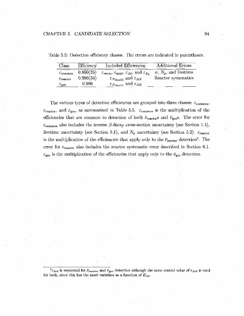
CHAPTER 5. CANDIDATE SELECTION 84
Table 5.5: Detection efficiency classes. The errors are indicated in parentheses.
Class Efficiency Included Efficiencies Additional Errors
common 0.860(35) £rec0n, £Spaii, eA t , and eEd °, Np, and livetime
factor 0.986(34) £ivMaxiD a n d £&R Reactor systematics
ggeo 0-986 giVMaxiD a n d £&R
The various types of detection efficiencies are grouped into three classes: ecommon,
£reactor, and egeo, as summarized in Table 5.5. eCommon is the multiplication of the
efficiencies that are common to detection of both factors and ^geos. The error for
common also includes the inverse /?-decay cross-section uncertainty (see Section 1.4),
livetime uncertainty (see Section 5.1), and iVp uncertainty (see Section 5.2). £reactor
is the multiplication of the efficiencies that apply only to the Reactor detection4. The
error for £reactor also includes the reactor systematic error described in Section 6.1.
£geo is the multiplication of the efficiencies that apply only to the iJgeo detection.
i£AR is separated for Reactor and v&eo detection although the same central value of £AA is used for both, since this has the most variation as a function of Ev{a.
Chapter 6
Signals and Backgrounds
The Candidate Selection Cuts described in Section 5.3 select inverse /^-decays and
their subsequent neutron captures from PreactorS and ugeos. After applying these cuts,
a number of background events are expected to remain in the candidate list. The
various event types are discriminated from each other using four observable quantities,
Ep, Ed, At, and t (absolute time). In this chapter, the expected rate and spectra, or
Probability Density Functions (PDFs) if normalized to unity, as a function of these
four variables for the signal and background event types are discussed.
6.1 Anti-Neutrinos from Nuclear Reactors
Most of the event-pairs that pass the Candidate Selection Cuts described in Sec
tion 5.3 are expected to be inverse /3-decays and their subsequent neutron captures
from PreactorS- As described in Section 1.3.1, the majority of Reactors are produced
from /3-decays following fission of 235U, 238U, 239Pu, and 241Pu in the nuclear reactor
and /3-decays of 106Rh and 144Pr in the reactor and in the spent fuel. Approximately
50 nuclear reactor cores operate in Japan located between 87 km and 830 km from the
KamLAND site, and the calculation of the expected &reaiCtor energy spectrum at the
KamLAND site requires the knowledge of Reactor contribution from each isotope in
each reactor. The instantaneous Reactor energy spectrum expected at the KamLAND
85
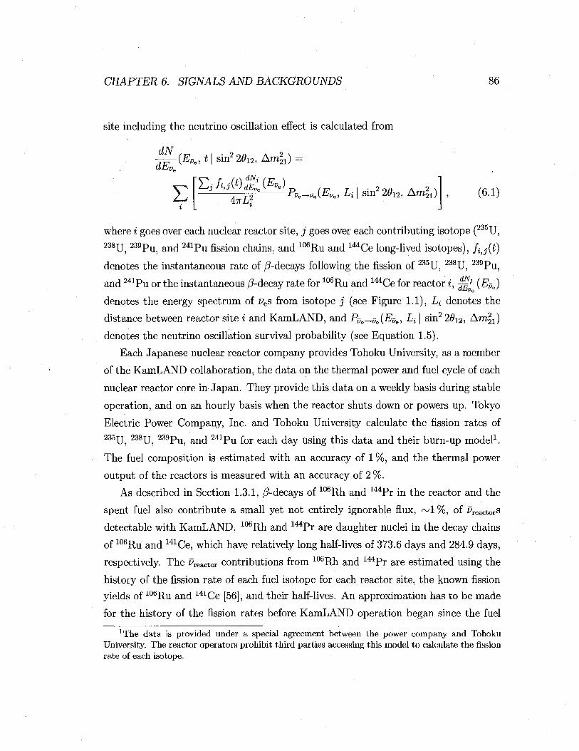
CHAPTER 6. SIGNALS AND BACKGROUNDS 86
site including the neutrino oscillation effect is calculated from
dN -(EQe, t |sin22012 , Am2
21)
£ dN, £^(')£(^)
4TTL? -Pp^9e(Eve, Li\sm226l2, Am2
21) (6.1)
where i goes over each nuclear reactor site, j goes over each contributing isotope (235U, 238U, 239Pu, and 241Pu fission chains, and 106Ru and 144Ce long-lived isotopes), fit j(t)
denotes the instantaneous rate of /3-decays following the fission of 235U, 238U, 239Pu,
and 241Pu or the instantaneous /?-decay rate for 106Ru and 144Ce for reactor i, -^-(E^)
denotes the energy spectrum of ves from isotope j (see Figure 1.1), Li denotes the
distance between reactor site i and KamLAND, and PPe^Pe(EPe, Lt | sin2 2#i2, Am^)
denotes the neutrino oscillation survival probability (see Equation 1.5).
Each Japanese nuclear reactor company provides Tohoku University, as a member
of the KamLAND collaboration, the data on the thermal power and fuel cycle of each
nuclear reactor core in Japan. They provide this data on a weekly basis during stable
operation, and on an hourly basis when the reactor shuts down or powers up. Tokyo
Electric Power Company, Inc. and Tohoku University calculate the fission rates of 235U, 238U, 239Pu, and 241Pu for each day using this data and their burn-up model1.
The fuel composition is estimated with an accuracy of 1 %, and the thermal power
output of the reactors is measured with an accuracy of 2 %.
As described in Section 1.3.1, /3-decays of 106Rh and 144Pr in the reactor and the
spent fuel also contribute a small yet not entirely ignorable flux, ~1 %, of z?reactorS
detectable with KamLAND. 106Rh and 144Pr are daughter nuclei in the decay chains
of 106Ru and 141Ce, which have relatively long half-lives of 373.6 days and 284.9 days,
respectively. The z>reactor contributions from 106Rh and 144Pr are estimated using the
history of the fission rate of each fuel isotope for each reactor site, the known fission
yields of 106Ru and 141Ce [56], and their half-lives. An approximation has to be made
for the history of the fission rates before KamLAND operation began since the fuel xThe data is provided under a special agreement between the power company and Tohoku
University. The reactor operators prohibit third parties accessing this model to calculate the fission rate of each isotope.
CHAPTER 6. SIGNALS AND BACKGROUNDS 87
cycle data for this period are not available. Constant fission rates of 235U, 238U, 239Pu, and 241Pu, obtained by averaging their fission rates in the first 9 months of
KamLAND operation, is assumed. The factors from the spent fuel are assumed to
traverse the same distance between the reactors, from which the fuel was removed,
and KamLAND since spent fuel is typically stored near the reactor for approximately
10 years, much longer than the half-lives of 106Ru and 141Ce.
The
reactor flux from nuclear reactors in Korea is estimated with a 10 % error
from the electricity generation records assuming that the fuel composition of Korean
reactors is the same as the average composition of the reactors in Japan. The factors
from the Korean reactors contribute approximately 3.4 % of the expected Reactor
flux
at the KamLAND site assuming no neutrino oscillation. The vreactOT flux contribution
from reactors outside of Japan and Korea are approximated with a 50% error by
placing one reactor for each country whose Reactor flux is estimated from the reported
electrical power produced in nuclear reactors. Together, all these reactors contribute
approximately 1% of the expected Reactor flux at the KamLAND site, assuming no
neutrino oscillation.
The total systematic error on the expected Preactor flux at the KamLAND site is
3.4 % obtained by combining the 1 % error from fuel composition uncertainty, the
2% error from thermal power uncertainty, the 0.6% error from the non-Japanese
reactor contribution uncertainty, and the 2.5 % error from the -^- uncertainty (see
Section 1.3.1). Note here that error on the Reactor flux is important for the sin22#i2
measurement, and has less effect on Am| x measurement since A m ^ is sensitive mostly
to the Ep spectral distortion.
The expected Ep spectrum for PreactorS is obtained by multiplying the Reactor energy
spectrum from Equation 6.1 with the inverse /?-decay cross-section (see Figure 1.6),
and converting the product into a Evis spectrum as discussed in Section 3.4. Figure 6.1
shows the expected Reactor Ep spectra for various neutrino oscillation parameters, ob
tained by using the central energy parameter values (see Section 3.4) and a detection
efficiency of 1, and separately integrating over period I and II.
The Ed and At PDFs are obtained from measurements of actual neutron captures
since the delayed events of the factor signal are captures of neutrons created in inverse
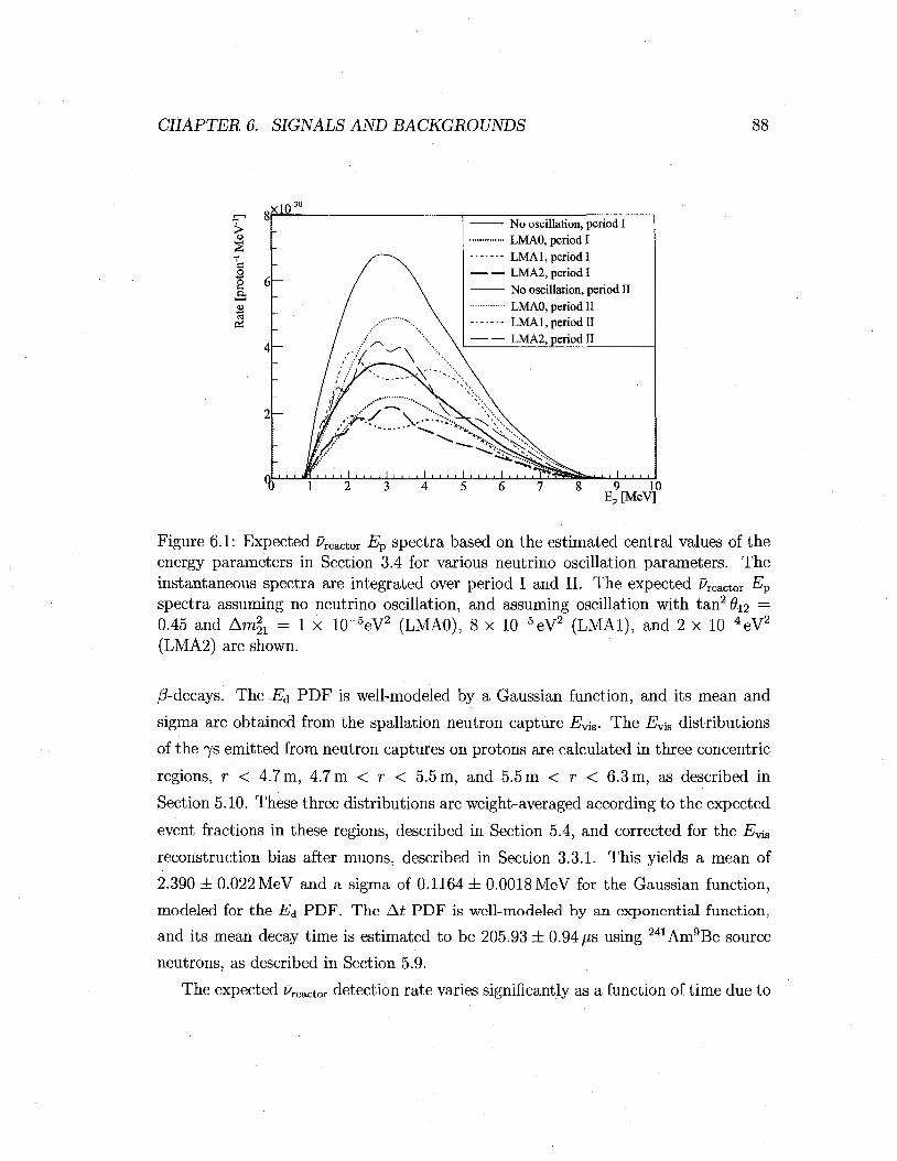
CHAPTER 6. SIGNALS AND BACKGROUNDS 88
No oscillation, period I LMAO, period I LMA1, period I LMA2, period I No oscillation, period II LMAO, period II LMAl,periodII
- LMA2, period II
Ep [MeV]
Figure 6.1: Expected Reactor Ep spectra based on the estimated central values of the energy parameters in Section 3.4 for various neutrino oscillation parameters. The instantaneous spectra are integrated over period I and II. The expected Reactor Ep
spectra assuming no neutrino oscillation, and assuming oscillation with tan2#i2 = 0.45 and A m | = 1 x l(T5eV2 (LMAO), 8 x 10"5eV2 (LMAl), and 2 x 10"4eV2
(LMA2) are shown.
/3-decays. The E& PDF is well-modeled by a Gaussian function, and its mean and
sigma are obtained from the spallation neutron capture Ev\a. The Ev{a distributions
of the 7s emitted from neutron captures on protons are calculated in three concentric
regions, r < 4.7 m, 4.7 m < r < 5.5 m, and 5.5 m < r < 6.3 m, as described in
Section 5.10. These three distributions are weight-averaged according to the expected
event fractions in these regions, described in Section 5.4, and corrected for the Evis
reconstruction bias after muons, described in Section 3.3.1. This yields a mean of
2.390 ± 0.022 MeV and a sigma of 0.1164 ± 0.0018 MeV for the Gaussian function,
modeled for the Ed P D F . The At P D F is well-modeled by an exponential function,
and its mean decay time is estimated to be 205.93 ± 0.94/is using 241Am9Be source
neutrons, as described in Section 5.9.
The expected factor detection rate varies significantly as a function of time due to
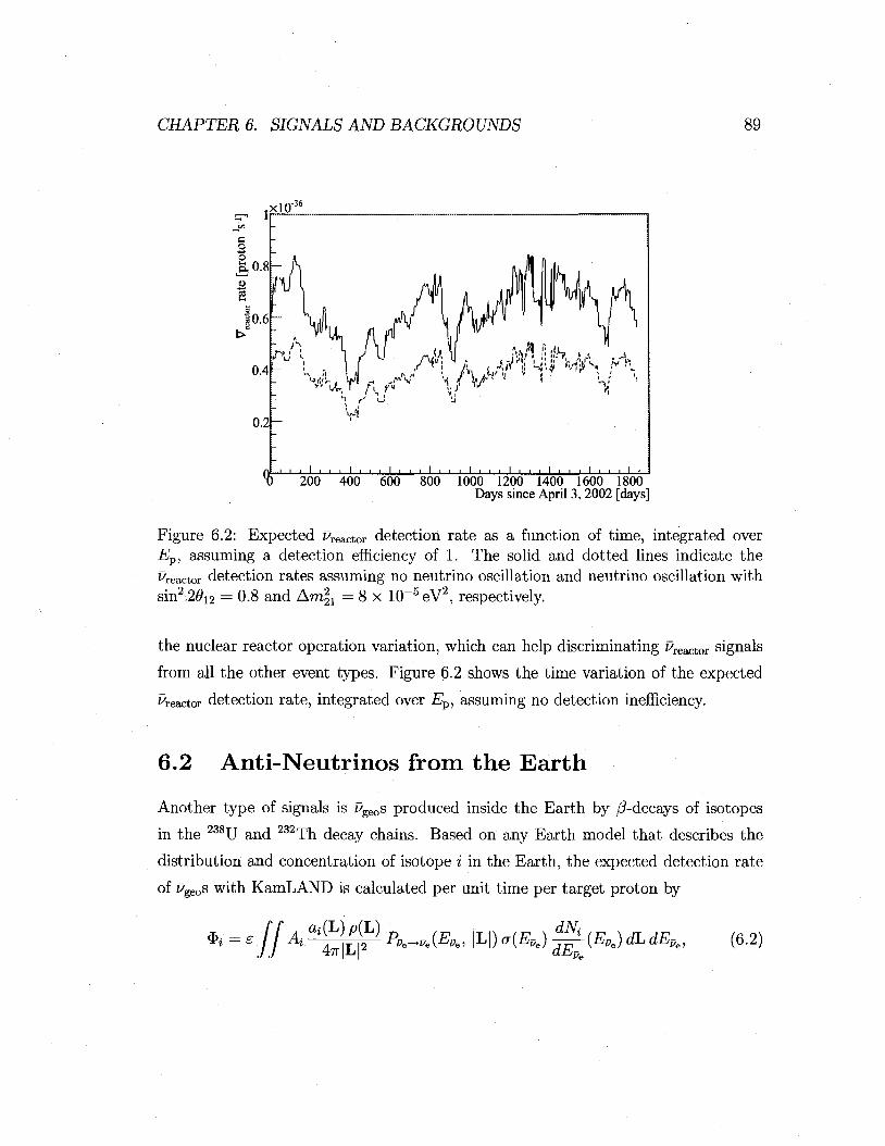
CHAPTER 6. SIGNALS AND BACKGROUNDS 89
kM^P^\rS
« _L _L I i i i I i i I i i i I
200 400 600 800 1000 1200 1400 1600 1800 Days since April 3,2002 [days]
Figure 6.2: Expected Reactor detection rate as a function of time, integrated over Ep, assuming a detection efficiency of 1. The solid and dotted lines indicate the reactor detection rates assuming no neutrino oscillation and neutrino oscillation with
sin22012 = 0.8 and Am|x = 8 x 10"5eV2, respectively.
the nuclear reactor operation variation, which can help discriminating Preactor signals
from all the other event types. Figure 6.2 shows the time variation of the expected
reactor detection rate, integrated over Ep, assuming no detection inefficiency.
6.2 Anti-Neutrinos from the Earth
Another type of signals is z/geos produced inside the Earth by /^-decays of isotopes
in the 238U and 232Th decay chains. Based on any Earth model that describes the
distribution and concentration of isotope i in the Earth, the expected detection rate
of zgeoS with KamLAND is calculated per unit time per target proton by
&* II <H(L) p(L) ITIWF ^ dNi (E9e)dLdEPe, (6.2)

CHAPTER 6. SIGNALS AND BACKGROUNDS 90
where e = eComraon^geo£Bp2) M denotes the decay rate per unit mass (Aa38u = 1.24 x
10 7s _ 1kg _ 1 and v4.232Th = 0.41 x 10 r s _ 1 kg _ 1 ) , L denotes the position relative to the
KamLAND site, Oj(L) denotes the isotope mass concentration at position L, p(L)
denotes the rock density, PVe^Pe(Epe, |L|) denotes the survival probability due to
neutrino oscillation (see Equation 1.5), o-(EPe) is the inverse /?-decay cross-section
(see Figure 1.6), and -^-(EcJ denotes the i/geo energy spectrum (see Figure 1.4).
The integral of dL is over the volume of the Earth, and the integral of dEpe is over
all energy. Since the production points of spread out within the Earth, the
sin2 (-—^2[Mevi ) ^ e r m m Poe-^pe(Ec,e, |L|) averages out to 0.5, and Equation 6.2
can be approximated with
*,«e (l-O.5sin22012) h J AaifJ^ dL, (6.3)
where
h = /'(Eri^iE^dEt
= 2.55 x 10"
or
Ve
— 2
44 ^geoS cm 238 U decay
-.2
Equation 6.3 can be rewritten as
$ i = £ ( l - 0.5 Sin2 2 0 i 2 ) ^effective,i, (6 .5)
where
^effective,* E= h j A* ^ j ^ ^ . (6 .6)
effective, i denotes the effective £5geo detection rate, independent of the detection effi
ciency and neutrino oscillation parameter, sin22012. Effective,? only depends on the
Earth model since the uncertainty on the inverse /3-decay cross-section is included
2£fip is applied during the fit. See Chapter 7 for more details.

CHAPTER 6. SIGNALS AND BACKGROUNDS 91
*
I
25 3 Ep [MeV]
Figure 6.3: 238U and 232Th ugeo Ep PDFs based on the estimated central values of the energy parameters in Section 3.4.
in the detection efficiency, as described in Section 5.11. Based on a,(L) and p(L)
derived from the Earth model described in Section 1.3.2, the expected effective, 238u
and Effective,232Th are 49 and 12 (1032p • y r ) _ 1 (per 1032 target protons per year),
respectively. If the Earth is "fully radiogenic," i.e., all the measured heat dissipation
rate at the surface of the Earth, 44.2 TW, comes from power generated by the ra
dioactivity in the Earth, <&effective, 238u a n d effective, 232Th can range from 79 to 114 and
19 to 28 (1032p • yr) _ 1 , respectively. Here, the lower bounds are the case where all
the excess radioactivity compared to the Earth model described in Section 1.3.2 is in
the mantle, and the upper bounds are the case where the radioactivity is fractionally
increased in the various sections of the Earth, while keeping the mass ratios among 232Th, 238U and other isotopes, mainly 40K, constant in both cases. Note here that
models with quite different Oj(L) and p(L) can be accommodated by the same data
if the resulting Effective, i a r e the same.
The expected Ep spectra for vgeo are obtained by converting the £>geo energy spectra
given in Figure 1.8 into Ev-m spectra as described in Section 3.4. Figure 6.3 shows the
CHAPTER 6. SIGNALS AND BACKGROUNDS 92
expected Vgeo Ep PDFs obtained by using the central values of the energy parameters
(see Section 3.4).
The Ed and At PDFs for neutron captures following the inverse /^-decays from
z>geos are the same as those from z>reactorS (see Section 6.1). Given that half-lives of 238U and 232Th are 4.47 x 10⁹ and 14.0 x 10⁹ years, respectively, and the timescale of
changes in the Earth structure is large, the t PDF for Pgeo is assumed to be constant.
6.3 Random Coincidence Background
The largest background arises from random coincidences; two uncorrelated events
from radioactivity in the LS that happened to be temporally and spatially nearby
can pass the Candidate Selection Cuts, described in Section 5.3.
The expected number and PDFs of such random event-pairs, iVrandom, is estimated
directly by using the data acquired in all the good runs:
-^random = N^t -Pother, (6 .7)
where N^t is the number of uncorrelated events that form timing coincidences, esti
mated using the events in all the good runs organized into multiplets (see Section 3.6).
-Pother is the probability of randomly paired events passing the Candidate Selection
Cuts (see Section 5.3), except the At Cut, and is estimated from
Pother = ^ , (6 .8) -''paired
where -/Vpaired denotes the number of randomly paired events, and iV0ther denotes the
number of these randomly paired events that pass the Candidate Selection Cuts,
except the At Cut.
Before events are randomly paired, a list of unpaired or "singles events" is gen
erated for each good run. To keep the data volume manageable, events that fail the
NMUXID Cut or Reconstruction Status Cut (see Section 5.3.1), or events with Ev{s
less than 0.8 MeV or reconstructed radius greater than 6.5 m are discarded from this

CHAPTER 6. SIGNALS AND BACKGROUNDS 93
| 2000
1500
1000
500
*0 1000 2000 3000 4000 5000 6000 Ar [mm]
Figure 6.4: Ar distributions of event-pairs in timing coincidence used for the N&t estimation (solid line), and a subset of randomly paired events counted for Arpaired
(dots with error bars). The distribution for the randomly paired events is normalized to the integral in the range of 1500 mm < Ar < 6000 mm.
singles event list. To ensure that N&t and P0ther are calculated from the same initial
event sets, these cuts also are applied to the events organized into multiplets, used
for the NAt estimation.
To avoid correlated events due to noisy periods or muons and their spallation
products from being counted in the estimation of N&t, the Multiplet Cut (see Sec
tion 5.3.1) and the Cosmogenic Spallation Cuts (see Section 5.3.2) are applied to the
events organized into multiplets. These cuts should also be applied to the singles
events to ensure that correlated events do not alter Pother- However, the Multiplet
Cut is difficult to apply to the singles events, so it is ignored. The consequence of
ignoring this cut is negligible since the overwhelming majority of singles events that
pass the Muon Cut, as a part of the Cosmogenic Spallation Cuts, would not form
a multiplet with more than 10 entries. The Muon Cylinder Cut is not applied to
the singles events at this stage since they do not have well-defined "prompt events,"
which are needed to apply this cut.
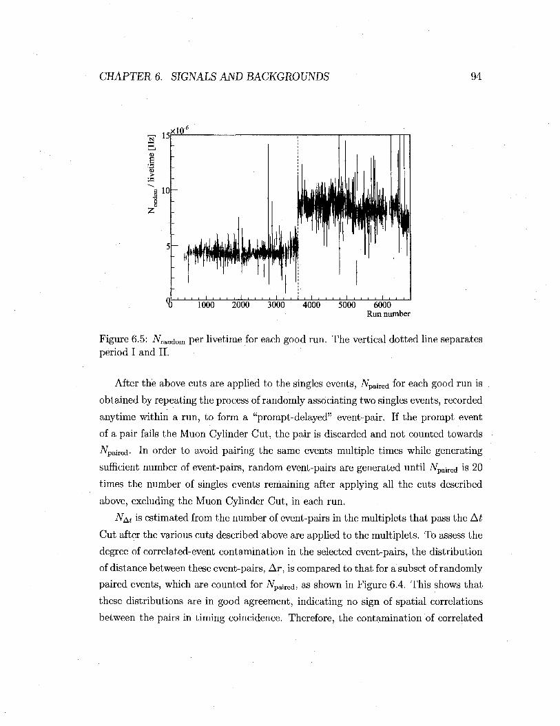
CHAPTER 6. SIGNALS AND BACKGROUNDS 94
N X
a >
15i xlO"'
I 10
<& 1000 2000 3000 4000 5000 6000 Run number
Figure 6.5: iVrandom per livetime for each good run. The vertical dotted line separates period I and II.
After the above cuts are applied to the singles events, iVpaired for each good run is
obtained by repeating the process of randomly associating two singles events, recorded
anytime within a run, to form a "prompt-delayed" event-pair. If the prompt event
of a pair fails the Muon Cylinder Cut, the pair is discarded and not counted towards
^paired- In order to avoid pairing the same events multiple times while generating
sufficient number of event-pairs, random event-pairs are generated until iVpaired is 20
times the number of singles events remaining after applying all the cuts described
above, excluding the Muon Cylinder Cut, in each run.
NAt is estimated from the number of event-pairs in the multiplets that pass the At
Cut after the various cuts described above are applied to the multiplets. To assess the
degree of correlated-event contamination in the selected event-pairs, the distribution
of distance between these event-pairs, Ar, is compared to that for a subset of randomly
paired events, which are counted for iVpaired, as shown in Figure 6.4. This shows that
these distributions are in good agreement, indicating no sign of spatial correlations
between the pairs in timing coincidence. Therefore, the contamination of correlated
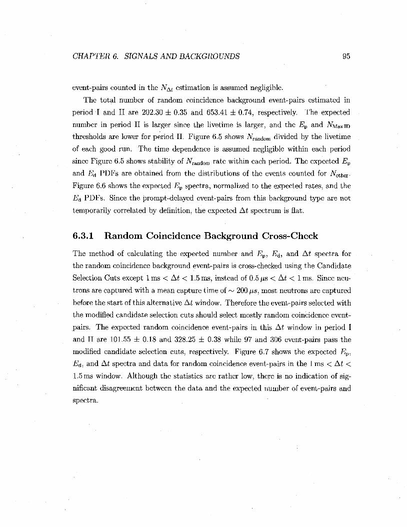
CHAPTER 6. SIGNALS AND BACKGROUNDS 95
event-pairs counted in the N^t estimation is assumed negligible.
The total number of random coincidence background event-pairs estimated in
period I and II are 202.30 ± 0.35 and 653.41 ± 0.74, respectively. The expected
number in period II is larger since the livetime is larger, and the Ep and AfMaxiD
thresholds are lower for period II. Figure 6.5 shows ATrandom divided by the livetime
of each good run. The time dependence is assumed negligible within each period
since Figure 6.5 shows stability of iVran(iom r a t e within each period. The expected Ep
and Ed PDFs are obtained from the distributions of the events counted for iVother.
Figure 6.6 shows the expected Ep spectra, normalized to the expected rates, and the
Ed PDFs. Since the prompt-delayed event-pairs from this background type are not
temporarily correlated by definition, the expected At spectrum is flat.
6.3.1 Random Coincidence Background Cross-Check
The method of calculating the expected number and Ep, E&, and At spectra for
the random coincidence background event-pairs is cross-checked using the Candidate
Selection Cuts except 1 ms < At < 1.5 ms, instead of 0.5 //s < At < 1 ms. Since neu
trons are captured with a mean capture time of ~ 200 /xs, most neutrons are captured
before the start of this alternative At window. Therefore the event-pairs selected with
the modified candidate selection cuts should select mostly random coincidence event-
pairs. The expected random coincidence event-pairs in this At window in period I
and II are 101.55 ± 0.18 and 328.25 ± 0.38 while 97 and 306 event-pairs pass the
modified candidate selection cuts, respectively. Figure 6.7 shows the expected Ep,
Ed, and At spectra and data for random coincidence event-pairs in the 1 ms < At <
1.5 ms window. Although the statistics are rather low, there is no indication of sig
nificant disagreement between the data and the expected number of event-pairs and
spectra.

CHAPTER 6. SIGNALS AND BACKGROUNDS 96
'10%
I . i r r T V V T 12 14
Ep [MeV]
•r- 2i
Figure 6.6: Random coincidence background Ep spectra normalized to the expected event rates (top plot) and Ed PDFs (bottom plot) for period I (solid thick line) and period II (dotted line).

CHAPTER 6. SIGNALS AND BACKGROUNDS 97
E™ [MeV]
650
600
550
500
• •
1 l 1 l
1 ( -
2.1 2.2 2.3 2.4 2.5 2.6 2.7 E „ [MeV]
e
•1 5- IOOO
1 900
800
600l=- — 1 - - J — 1 — 1 — 1—L-- J— L — L - J — I — J — L . J — J — I - - J — 1 — I - . I
1.05 1.1 1.15 1.2 1.25 1.3 1.35 1.4 1.45 1.5 At [ms]
Figure 6.7: Random coincidence background spectra cross-check. The top, middle, and bottom plots show Ep, E&, and At spectra, respectively. The data points are for the event-pairs which pass the Candidate Selection Cuts except that At is chosen from 1ms < At < 1.5 ms. The solid curves are the expected spectra for the random coincidence event-pairs in the lms < At < 1.5 ms window.

CHAPTER 6. SIGNALS AND BACKGROUNDS 98
6.4 13C(a, n) Background
Radioactivity in the detector causes another type of backgrounds, "13C(o;, n) back
ground events." a particles can sometimes interact with naturally occurring 13C in the
LS, causing 13C(a, n) reactions, which combined with the thermalization and capture
of the produced neutron can mimic prompt-delayed event-pairs from inverse /3-decays
and their subsequent neutron captures.
The main source of a particles is 210Po decays in the LS. 222Rn, which was
unintentionally introduced into the detector during the detector construction, has
decayed into 2 1 0Pb. This 210Pb is distributed throughout the detector and decays
into 210Po with a half-life of 22.3 years3. With a half-life of 138 days, the 210Po a-
decays, producing a particles with a kinetic energy of 5.3 MeV, which is quenched to
Evis of ~0.3 MeV, well below the analysis Evia threshold. However, when a particles
interact with 13C, they can cause events with high enough Ev[8 to be seen above the
threshold.
With an initial a energy of 5.3 MeV, the 13C(a, n) reaction can produce 1 6 0 in the
ground, first, or second excited state. When 1 6 0 is created in the ground state, the
neutron is emitted with energy between ~2.5 and ~7.5 MeV. Most of the neutrons
thermalize via elastic scatterings with protons. However, some high energy neutrons
can also lose energy via inelastic scattering with a 12C, emitting a 4.439 MeV 7. When 1 6 0 is created in the first excited state, the 1 6 0 returns to the ground state by internal
pair conversion, emitting an electron-positron pair with a total energy of 6.049 MeV.
When 1 6 0 is created in the second excited state, the 1 6 0 returns to the ground state
by emitting a 6.130 MeV 7. The neutrons created in the 13C(a, n)1 60* reactions,
which have very low energy, thermalize via elastic scatterings.
Event rate of 13C(a, n) reactions depends on activity of the 210Po a-decays, which
can be estimated from a peak in the i?vis spectrum caused by the a particles. Since
-Evis of the a particles is very low, ~0.3 MeV, the EviS reconstruction algorithm may
not have high enough reconstruction efficiency or accuracy for the 210Po activity
measurement. Instead, the activity of the 210Po a-decays is estimated using the
3See Figure 1.3 for the decay chain of 222Rn that eventually decays to 210Po.
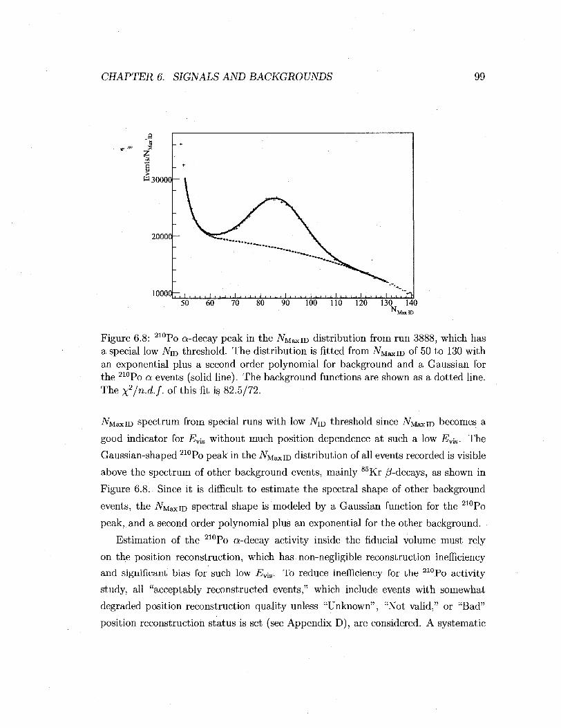
CHAPTER 6. SIGNALS AND BACKGROUNDS 99
'• •'• I ' ' •- -«---! I l ' I...1...I..I .1 1.1 I I 1 ...I I I I I ...J ...J I I I l - l . - l - l . . I_ I .J . .J . . l_ l - i - l . . . l . . . l . .±-L- lJ
50 60 70 80 90 100 110 120 130 140
Figure 6.8: 210Po a-decay peak in the iVMaxiD distribution from run 3888, which has a special low iVID threshold. The distribution is fitted from iVMaxID of 50 to 130 with an exponential plus a second order polynomial for background and a Gaussian for the 210Po a events (solid line). The background functions are shown as a dotted line. The xVn.d.f. of this fit is 82.5/72.
'- MaxiD spectrum from special runs with low iVID threshold since iVMaxID becomes a
good indicator for Evis without much position dependence at such a low Ev{s. The
Gaussian-shaped 210Po peak in the iVMaxID distribution of all events recorded is visible
above the spectrum of other background events, mainly 85Kr /^-decays, as shown in
Figure 6.8. Since it is difficult to estimate the spectral shape of other background
events, the A^axiD spectral shape is modeled by a Gaussian function for the 210Po
peak, and a second order polynomial plus an exponential for the other background.
Estimation of the 210Po a-decay activity inside the fiducial volume must rely
on the position reconstruction, which has non-negligible reconstruction inefficiency
and significant bias for such low EV-1S. To reduce inefficiency for the 210Po activity
study, all "acceptably reconstructed events," which include events with somewhat
degraded position reconstruction quality unless "Unknown", "Not valid," or "Bad"
position reconstruction status is set (see Appendix D), are considered. A systematic
0 s s
? a a> > W30000
20000
10000
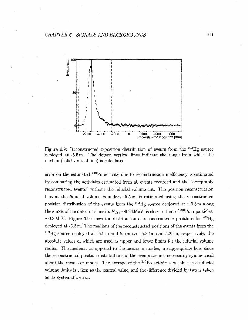
CHAPTER 6. SIGNALS AND BACKGROUNDS 100
lOOi
a >
50
,
J_
'\ W, M^tyN^^
_L -6000 -4000 -2000
_ 1 I I L .
0 2000 4000 6000 Reconstructed z position [mm]
Figure 6.9: Reconstructed z-position distribution of events from the 203Hg source deployed at -5.5 m. The dotted vertical lines indicate the range from which the median (solid vertical line) is calculated.
error on the estimated 210Po activity due to reconstruction inefficiency is estimated
by comparing the activities estimated from all events recorded and the "acceptably
reconstructed events" without the fiducial volume cut. The position reconstruction
bias at the fiducial volume boundary, 5.5 m, is estimated using the reconstructed
position distribution of the events from the 203Hg source deployed at ±5.5 m along
the z-axis of the detector since its Evis, ~0.24MeV, is close to that of 210Po a particles,
~0.3MeV. Figure 6.9 shows the distribution of reconstructed z-positions for 203Hg
deployed at -5.5 m. The medians of the reconstructed positions of the events from the 203Hg source deployed at -5.5 m and 5.5 m are -5.32 m and 5.25 m, respectively, the
absolute values of which are used as upper and lower limits for the fiducial volume
radius. The medians, as opposed to the means or modes, are appropriate here since
the reconstructed position distributions of the events are not necessarily symmetrical
about the means or modes. The average of the 210Po activities within these fiducial
volume limits is taken as the central value, and the difference divided by two is taken
as its systematic error.
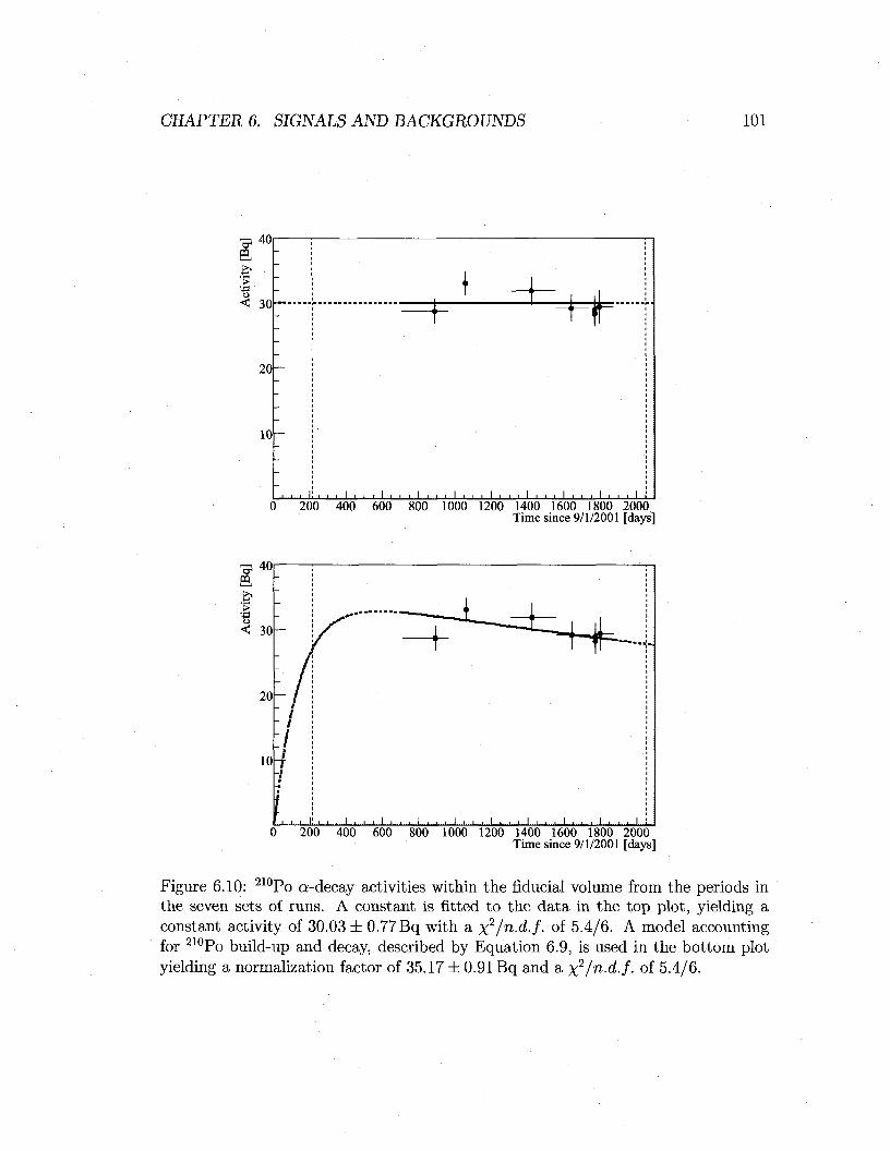
CHAPTER 6. SIGNALS AND BACKGROUNDS 101
m
< 30H Hr 20h
10h
i i i i i i I i
0 200 400 600 800 1000 1200 1400 1600 1800 2000 Time since 9/1/2001 [days]
200 400 600 800 1000 1200 1400 1600 1800 2000 Time since 9/1/2001 [days]
Figure 6.10: 210Po a-decay activities within the fiducial volume from the periods in the seven sets of runs. A constant is fitted to the data in the top plot, yielding a constant activity of 30.03 ± 0.77 Bq with a x 2 /n .d / . of 5.4/6. A model accounting for 210Po build-up and decay, described by Equation 6.9, is used in the bottom plot yielding a normalization factor of 35.17 ± 0.91 Bq and a y^/n.d.f. of 5.4/6.

CHAPTER 6. SIGNALS AND BACKGROUNDS 102
Table 6.1: Fitted 210Po a-decay activities in seven sets of runs. The fitted numbers of 210Po a-decays are divided by the livetimes. The values in the second column are from all events recorded, and those in the third column are from the "acceptably reconstructed events." The activities within the fiducial volume are estimated using the lower (4th column) and upper (5th column) limits for the fiducial volume radius corresponding to 5.5 m for 210Po a-decays.
Run number
2783 to 3615 3888 4493 to 5147 5152 to 5671 5757 5767 5778 to 6276
All [Bq]
83.6 ±2.3 94.3 ±2.1 92.7 ±2.6 91.8 ±2.5 88.6 ± 2.4 90.1 ±2.3 85.4 ±3.2
Reconstructed [Bq]
83.1 ±2.3 94.1 ±2.3 90.9 ±2.7 89.7 ±2.5 86.3 ± 2.4 88.2 ±2.4 82.7 ±3.1
r < 5.25 m [Bq]
28.2 ±1.3 32.5 ±1.2 31.3 ±1.4 28.5 ±1.3 28.3 ±1.3 27.7 ±1.2 28.9 ± 1.9
r < 5.32 m [Bq]
29.3 ±1.3 33.7 ±1.2 32.5 ±1.5 29.9 ±1.3 29.6 ± 1.4 28.9 ±1.2 29.8 ±1.9
There are many low-iVID threshold runs throughout the data-set analyzed in this
thesis. These runs are divided into seven sets, by combining short runs to gain statis
tics while leaving three long runs by themselves. For each set, the activities of 210Po
a-decays are estimated as shown in Table 6.1. As a function of time since September
1st, 2001, Figure 6.10 shows the estimated 210Po activities inside the fiducial volume,
including the systematic errors due to the position reconstruction efficiency and bias
calculated for each set of runs. The top plot shows a fit to a constant yielding an
average 210Po activity within the fiducial volume of 30.03 ± 0.77 Bq. The bottom plot
in Figure 6.10 shows the fit to the model of the activity build-up and decay described
by the function:
A ABi APo x
(Apb — ABO (Ap0 — Aei) (Apb — Ap0) (Asi — Apc) J
where ABJ, AP O , and APb denote the decay constants for 210Bi, 210Po, and 210Pb,
respectively, and A denotes the normalization, which is the fitted parameter. Based
[(Am-
(Apb -
g—APb t
- APb) (APo — Apb)
- ABJ) (Apo — Aei) (Apb -
p—Ap01
- Ap0) (Asi -- Ap0)

CHAPTER 6. SIGNALS AND BACKGROUNDS 103
Table 6.2: Estimated total 210Po a-decays for various background functions from run 3888, which has a special low iVjD threshold. The first column is the functions used to fit the background, where oo, ai, a2, b, and c are fitted. The third column, Probability, is the probability based on the -y^/n.d.f. of the fit.
Background function
a$ + ai x a0 + ai x + a2 x
2
a0 + aix + a2 x2
a0 + aix + a2 x2
cio + aix + becx
a0 + % x + a2 £2
a0 + ai a; + a2 a;2 + 6ec* + 6eca:
iVMaxiD limits 60 to 105 60 to 120 60 to 125 60 to 130 50 to 105 50 to 125 50 to 130
Probability 0.13 0.11 0.15
.0.14 0.12 0.21 0.19
Fitted 210Po decays
(2.411 ±0.088) x 105
(2.34 ±0.13) x 105
(2.347 ±0.076) x 105
(2.249 ± 0.049) x 105
(2.50 ±0.10) x 105
(2.405 ± 0.080) x 105
(2.308 ± 0.056) x 105
on this fit, the average 210Po decay activity within the fiducial volume in the analysis
period is 31.33 ± 0.81 Bq. Therefore, the activities estimated using the constant fit
and this model are consistent. The value from the constant fit is used in the analysis,
and the difference between the two different fit functions is taken as a systematic
error.
An additional systematic error comes from the assumption that the iVMaxiD spec
trum of the other background events is modeled simply by a second order polynomial
plus an exponential. Various functions and fit limits are tried to estimate the vari
ation in the number of 210Po a-decay events estimated using all the events recorded
in special run 3888, which has a Nm threshold of 35. Only four functions give a
reasonable fit that yields convergence, an accurate error matrix, and a fit probability
greater than 0.1, based on the \2/n.d.f. Table 6.2 summarizes the fitted numbers
of 210Po a-decay events, and probabilities for various reasonable fit functions. The
percentage difference between the maximum and minimum numbers of 210Po a-decay
events fitted is ~11%, which is included in the error on the 210Po activity, yielding
30.0 ± 3.5 Bq.

CHAPTER 6. SIGNALS AND BACKGROUNDS 104
The number of neutrons produced per a particle, Y, is given by
F = p / ^ ^ - = ( 6 . 0 ± 0 . 3 ) x l 0 - 8 , (6.10)
where p = 3.7 x 10²⁰ c m - 3 denotes the density of 13C in the target, cr(E) denotes the
reaction cross-section [57], ^ (E) denotes the a particle stopping power [58], and Ea
denotes the maximum kinetic energy of the a particle. The error is estimated from
comparison between a calculation using C targets with natural C isotope composi
tions and measurements [59]. Combining the estimated 210Po activity, the number
of neutrons produced per a particle (Y), and a detection efficiency, the expected 13C(a, n) background rate is estimated to be (1.53 ±0.20) x 10~6 per second in the
entire £v i s range. The detection efficiency here includes £jvMaxiD, Brecon, £Spaii, £AK, £A*,
and £Ed4, and is assumed to be constant in Ep even below the Ep analysis threshold;
although the actual efficiency drops significantly below Ep threshold mostly due to
the NMaxiD Cut, the difference between the assumed constant efficiency and actual ef
ficiency below the Ep threshold becomes irrelevant once the Ep Cut is applied during
the analysis fit, described in Section 7.2.
As described in the beginning of this section, 210Po a particles can cause 13C(«, n)
reactions that result in thermalization of neutrons via elastic scatterings alone, or
those combined with inelastic scattering with 12C, or de-excitation of 1 60*. The
fraction of each reaction type is estimated by simulating 104 13C(a, n) reactions using
the cross-sections for the 13C(o!, n) reactions, inelastic scattering of a neutron with a 12C, and elastic scattering of a neutron with a proton and a 12C. This simulation yields
88640 events with only neutron elastic scattering, 2105 events with a 12C inelastic
scattering, and 9256 events with 1 6 0* de-excitation. Using the number of events in
each reaction type, the ratio of the number of the inelastic 12C scattering events to the
total is estimated to be 0.02105 ± 0.00045, where the error comes from the statistical
error on the simulated number of events. The ratio of the number of 1 3C(a, n)1 60*
events to total is estimated to be 0.09 ± 0.09, where a 100% error is assigned to this
4Since EEP is calculated during the fit, it is not included in this estimate.
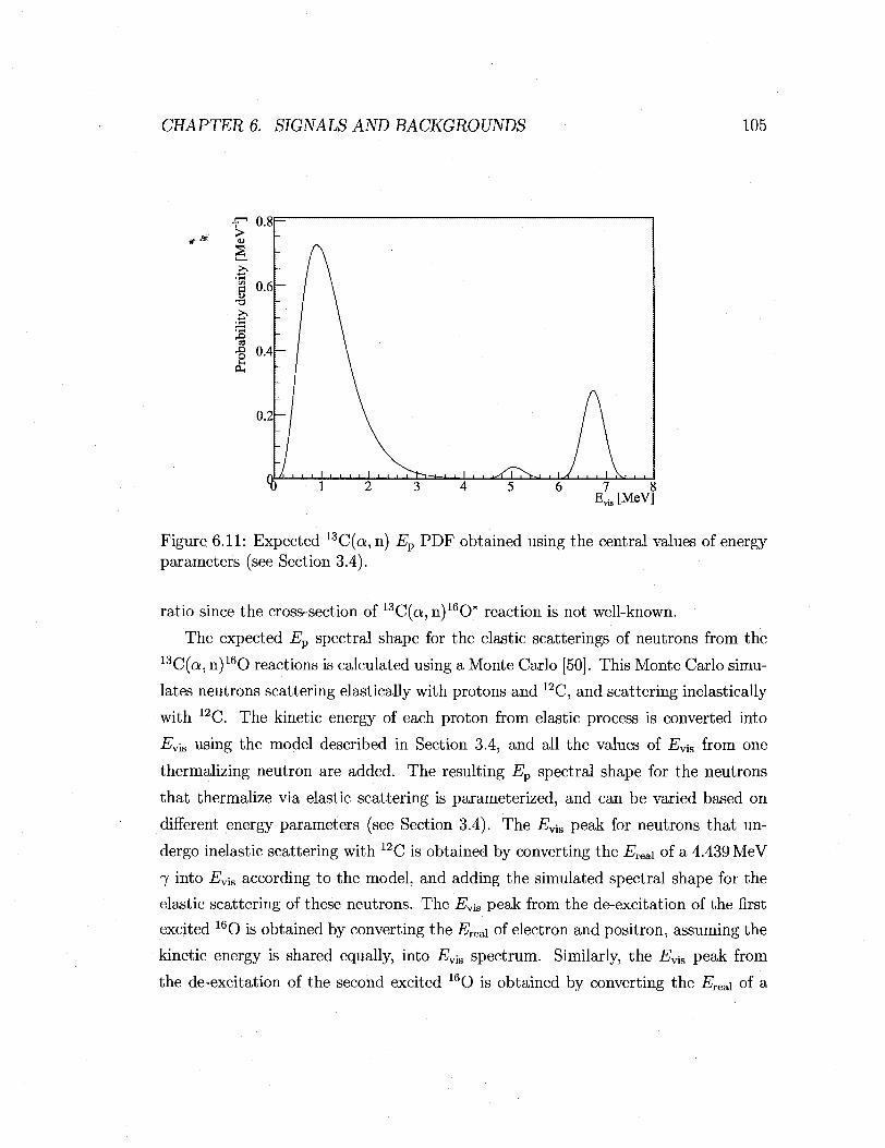
CHAPTER 6. SIGNALS AND BACKGROUNDS 105
Evis [MeV]
Figure 6.11: Expected 13C(a, n) Ep PDF obtained using the central values of energy parameters (see Section 3.4).
ratio since the cross-section of lsC(a, n)1 60* reaction is not well-known.
The expected Ep spectral shape for the elastic scatterings of neutrons from the 13C(a, n) 1 6 0 reactions is calculated using a Monte Carlo [50]. This Monte Carlo simu
lates neutrons scattering elastically with protons and 12C, and scattering inelastically
with 12C. The kinetic energy of each proton from elastic process is converted into
Evis using the model described in Section 3.4, and all the values of .E^ from one
thermalizing neutron are added. The resulting Ep spectral shape for the neutrons
that thermalize via elastic scattering is parameterized, and can be varied based on
different energy parameters (see Section 3.4). The Evia peak for neutrons that un
dergo inelastic scattering with 12C is obtained by converting the Eiea\ of a 4.439 MeV
7 into Evis according to the model, and adding the simulated spectral shape for the
elastic scattering of these neutrons. The .Evis peak from the de-excitation of the first
excited 1 6 0 is obtained by converting the Erea,\ of electron and positron, assuming the
kinetic energy is shared equally, into Ev[s spectrum. Similarly, the Ev\s peak from
the de-excitation of the second excited 1 6 0 is obtained by converting the Erea_\ of a
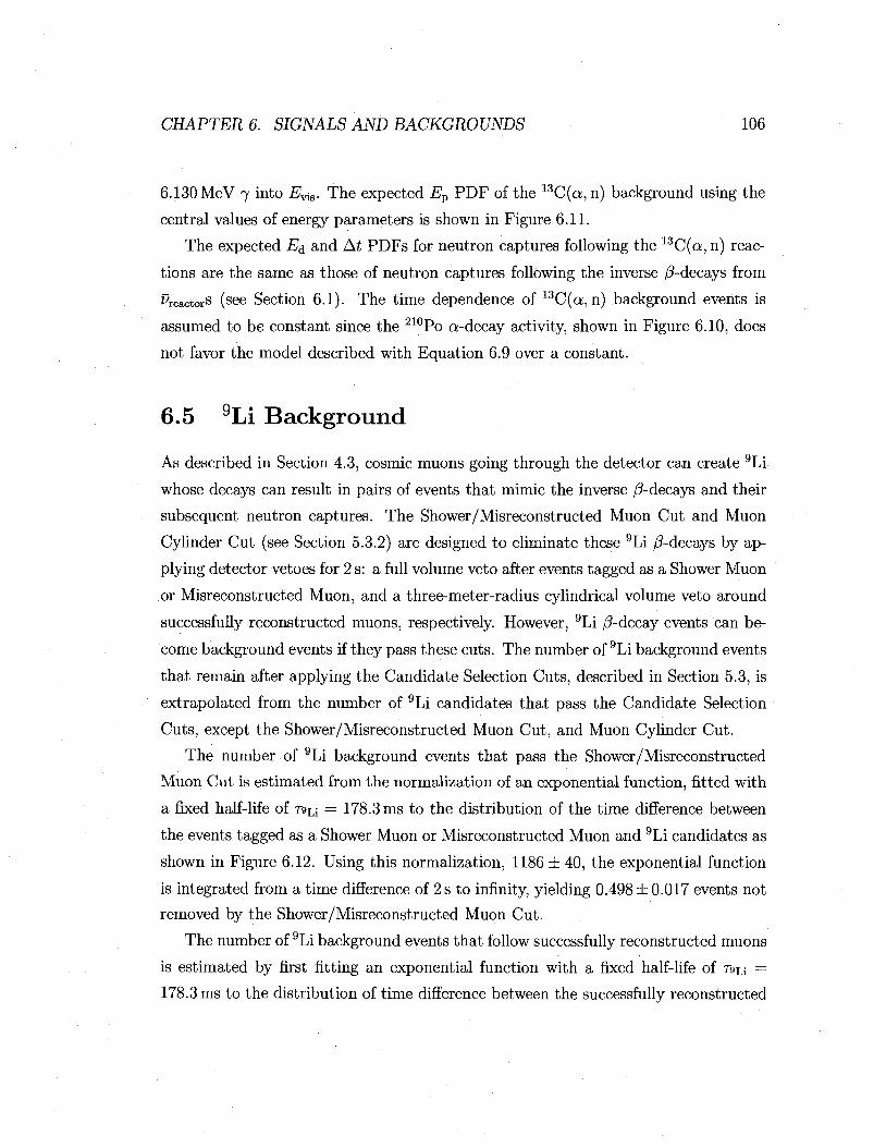
CHAPTER 6. SIGNALS AND BACKGROUNDS 106
6.130 MeV 7 into Evis. The expected Ep PDF of the 13C(a, n) background using the
central values of energy parameters is shown in Figure 6.11.
The expected Ed and At PDFs for neutron captures following the 13C(a, n) reac
tions are the same as those of neutron captures following the inverse /^-decays from
Reactors (see Section 6.1). The time dependence of 13C(a, n) background events is
assumed to be constant since the 210Po a-decay activity, shown in Figure 6.10, does
not favor the model described with Equation 6.9 over a constant.
6.5 9Li Background
As described in Section 4.3, cosmic muons going through the detector can create 9Li
whose decays can result in pairs of events that mimic the inverse /^-decays and their
subsequent neutron captures. The Shower/Misreconstructed Muon Cut and Muon
Cylinder Cut (see Section 5.3.2) are designed to eliminate these 9Li /^-decays by ap
plying detector vetoes for 2 s: a full volume veto after events tagged as a Shower Muon
or Misreconstructed Muon, and a three-meter-radius cylindrical volume veto around
successfully reconstructed muons, respectively. However, 9Li /?-decay events can be
come background events if they pass these cuts. The number of 9Li background events
that remain after applying the Candidate Selection Cuts, described in Section 5.3, is
extrapolated from the number of 9Li candidates that pass the Candidate Selection
Cuts, except the Shower/Misreconstructed Muon Cut, and Muon Cylinder Cut.
The number of 9Li background events that pass the Shower/Misreconstructed
Muon Cut is estimated from the normalization of an exponential function, fitted with
a fixed half-life of T9U = 178.3 ms to the distribution of the time difference between
the events tagged as a Shower Muon or Misreconstructed Muon and 9Li candidates as
shown in Figure 6.12. Using this normalization, 1186 ± 40, the exponential function
is integrated from a time difference of 2 s to infinity, yielding 0.498 ±0.017 events not
removed by the Shower/Misreconstructed Muon Cut.
The number of 9Li background events that follow successfully reconstructed muons
is estimated by first fitting an exponential function with a fixed half-life of TQU =
178.3 ms to the distribution of time difference between the successfully reconstructed

CHAPTER 6. SIGNALS AND BACKGROUNDS 107
_L . - • - — L . . . - 1 . I 1 | | _ _L —1- - I . . - . . J - . . . 1 l l | _ • » ' • • •
0.2 0.4 0.6 0.8 1.2 1.4 1.6 1.8 2 Time since muons [s]
Figure 6.12: Time between muons and spallation 9Li /3-decay events. The filled circles are for 9Li /3-decay events obtained by reversing the Muon Cylinder Cut, and the open circles are for those after events tagged as Shower Muons or Misreconstructed Muons. The solid lines indicate fits to an exponential function plus a constant, using the nominal half-life of 9Li /?-decay, 178.3 ms. The fitted number of 9Li decays and X2/n.d.f. for those obtained by reversing the Muon Cylinder Cut are 41 ± 11 and 29.4/28, respectively. The fitted numbers of 9Li decays and %2 jn.d.f. for those after events tagged as Shower Muons or Misreconstructed Muons are 1186±40 and 29.1/28, respectively.
muons and 9Li candidates whose position is reconstructed within 3 m from the recon
structed muon track, as shown in Figure 6.12. Using the fitted normalization, 41 ± 12,
the number of events outside the cylinder around the muon tracks is obtained from
2s
^cylinder = (41 ± 12) Rout/in — f e X P ( - — t] dt, (6 .11)
2 ms
where i?out/in is the ratio of 9Li /?-decay events expected to be outside to inside of
the 3 m cylinder around the muons. .Rout/in is estimated from spallation neutrons
produced by muons with successfully reconstructed tracks. Figure 6.13 shows the
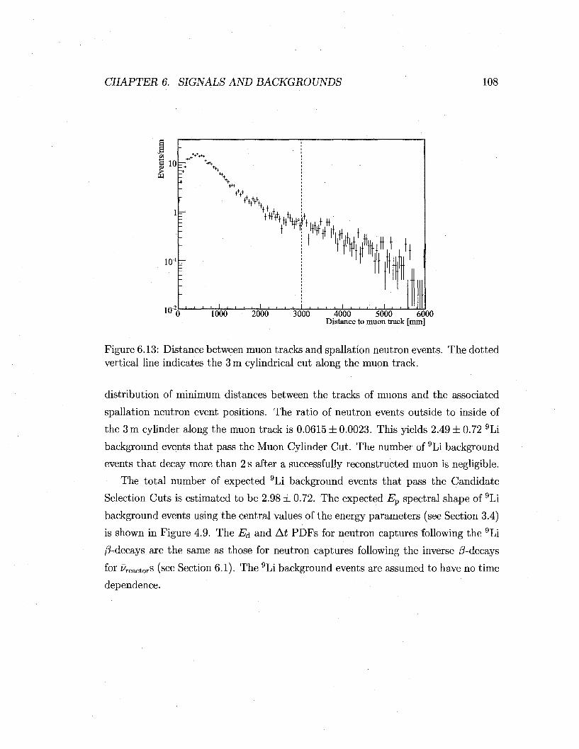
CHAPTER 6. SIGNALS AND BACKGROUNDS 108
, • » ! . . . . I . . . . , , , , I , , , , I , , l,",l 1U 0 1000 2000 3000 4000 5000 6000
Distance to muon track [mm]
Figure 6.13: Distance between muon tracks and spallation neutron events. The dotted vertical line indicates the 3 m cylindrical cut along the muon track.
distribution of minimum distances between the tracks of muons and the associated
spallation neutron event positions. The ratio of neutron events outside to inside of
the 3 m cylinder along the muon track is 0.0615 ± 0.0023. This yields 2.49 ± 0.72 9Li
background events that pass the Muon Cylinder Gut. The number of 9Li background
events that decay more than 2 s after a successfully reconstructed muon is negligible.
The total number of expected 9Li background events that pass the Candidate
Selection Cuts is estimated to be 2.98 ± 0.72. The expected Ep spectral shape of 9Li
background events using the central values of the energy parameters (see Section 3.4)
is shown in Figure 4.9. The E& and At PDFs for neutron captures following the 9Li
/3-decays are the same as those for neutron captures following the inverse /3-decays
for Reactors (see Section 6.1). The 9Li background events are assumed to have no time
dependence.
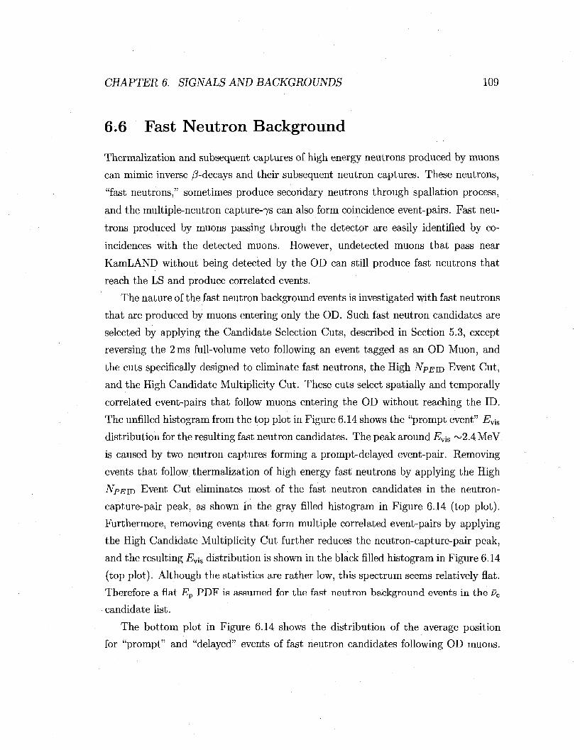
CHAPTER 6. SIGNALS AND BACKGROUNDS 109
6.6 Fast Neutron Background
Thermalization and subsequent captures of high energy neutrons produced by muons
can mimic inverse /^-decays and their subsequent neutron captures. These neutrons,
"fast neutrons," sometimes produce secondary neutrons through spallation process,
and the multiple-neutron c a p t u r e ^ can also form coincidence event-pairs. Fast neu
trons produced by muons passing through the detector are easily identified by co
incidences with the detected muons. However, undetected muons that pass near
KamLAND without being detected by the OD can still produce fast neutrons that
reach the LS and produce correlated events.
The nature of the fast neutron background events is investigated with fast neutrons
that are produced by muons entering only the OD. Such fast neutron candidates are
selected by applying the Candidate Selection Cuts, described in Section 5.3, except
reversing the 2 ms full-volume veto following an event tagged as an OD Muon, and
the cuts specifically designed to eliminate fast neutrons, the High Npsm Event Cut,
and the High Candidate Multiplicity Cut. These cuts select spatially and temporally
correlated event-pairs that follow muons entering the OD without reaching the ID.
The unfilled histogram from the top plot in Figure 6.14 shows the "prompt event" Ev-iS
distribution for the resulting fast neutron candidates. The peak around Evva ~2.4 MeV
is caused by two neutron captures forming a prompt-delayed event-pair. Removing
events that follow thermalization of high energy fast neutrons by applying the High
NPEID Event Cut eliminates most of the fast neutron candidates in the neutron-
capture-pair peak, as shown in the gray filled histogram in Figure 6.14 (top plot).
Furthermore, removing events that form multiple correlated event-pairs by applying
the High Candidate Multiplicity Cut further reduces the neutron-capture-pair peak,
and the resulting Evia distribution is shown in the black filled histogram in Figure 6.14
(top plot). Although the statistics are rather low, this spectrum seems relatively flat.
Therefore a flat Ep PDF is assumed for the fast neutron background events in the Pe
candidate list.
The bottom plot in Figure 6.14 shows the distribution of the average position
for "prompt" and "delayed" events of fast neutron candidates following OD muons.
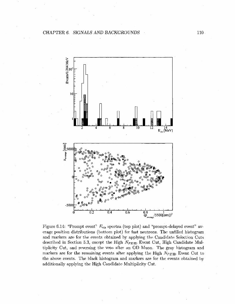
CHAPTER 6. SIGNALS AND BACKGROUNDS 110
i 10 1 i
12 14 E^JMeV]
£5000
-5000
o
.
e
- C
3
. f t O S
OB ^
O -o 0 o O O o
o°°<5> gCXBjrfDO
= 0
o o q 3 9
°o o° °0 °
0 „ o °
° <?° ^ S b o d ^ f d ^
, , 1
o
1 1 1 1 I t i l l 1 1 1 1 1 1 1
0.2 0.4 0.6 (p /5500[mm])2
Figure 6.14: "Prompt event" Evis spectra (top plot) and "prompt-delayed event" average position distributions (bottom plot) for fast neutrons. The unfilled histogram and markers are for the events obtained by applying the Candidate Selection Cuts described in Section 5.3, except the High NPEiD Event Cut, High Candidate Multiplicity Cut, and reversing the veto after an OD Muon. The gray histogram and markers are for the remaining events after applying the High NPE ID Event Cut to the above events. The black histogram and markers are for the events obtained by additionally applying the High Candidate Multiplicity Cut.

CHAPTER 6. SIGNALS AND BACKGROUNDS 111
The unfilled markers indicate the average positions of the fast neutron candidates
including those following high energy fast neutrons. These reach deep into the LS
although they are slightly more concentrated around the fiducial volume boundary.
Removing events following high energy fast neutrons eliminates many of the events
that reach the center of the ID, as shown in the gray filled markers in the bottom plot
in Figure 6.14, because high energy fast neutrons have a longer attenuation length.
Removing events that form multiple correlated event-pairs results in the black filled
markers in Figure 6.14 (bottom plot). These events may be somewhat concentrated
around the equator, where the OD is the thinest, and therefore the buffer between
the surrounding rock and the ID is thinest, making it easier for fast neutrons to
penetrate into the LS. Since the OD is the least efficient in detecting muons going
near the thinnest part of the OD, there may be quite a few fast neutrons that are
not associated with detected muons. Since the efficiency of detecting such muons is
not well understood, the expected number of fast neutrons that pass the Candidate
Selection Cuts is not estimated directly. Instead, the PDF normalization is allowed to
freely float to match the selected ue candidate distribution, as described in Section 7.2.
The Ed and At PDFs for neutron captures following the thermalization of fast
neutrons or other captures of neutrons produced from the same muons are the same
as those for neutron captures following the inverse /3-decays from Preactors (see Sec
tion 6.1). The fast neutron background events are assumed to have no time depen
dence.
6.7 Atmospheric v Background
A possible source of background is from quasi-elastic neutral current interaction of
atmospheric us with neutrons in 12C nuclei. The recoil neutron produces a prompt
event, and its capture produces the delayed event. The atmospheric u background
events are studied using a KLG4sim simulation [60]. For simplicity, this simulation
assumes that atmospheric us interact with free neutrons, neglecting nuclear effects of 12C. Therefore the result of this simulation is treated as a very rough estimation. The
cross-section for interactions between a u and a neutron is obtained by modifying the
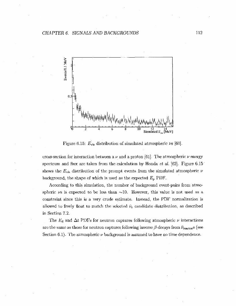
CHAPTER 6. SIGNALS AND BACKGROUNDS 112
10 12 14 Simulated E . [MeV]
Figure 6.15: Ev-iS distribution of simulated atmospheric MS [60].
cross-section for interaction between a v and a proton [61]. The atmospheric v energy
spectrum and flux are taken from the calculation by Honda et al. [62]. Figure 6.15
shows the Ev-m distribution of the prompt events from the simulated atmospheric v
background, the shape of which is used as the expected Ep PDF.
According to this simulation, the number of background event-pairs from atmo
spheric us is expected to be less than ^10. However, this value is not used as a
constraint since this is a very crude estimate. Instead, the PDF normalization is
allowed to freely float to match the selected ue candidate distribution, as described
in Section 7.2.
The Ed and At PDFs for neutron captures following atmospheric v interactions
are the same as those for neutron captures following inverse /^-decays from reactor13 (see
Section 6.1). The atmospheric v background is assumed to have no time dependence.
Chapter 7
Likelihood Analysis and Results
This analysis simultaneously estimates the neutrino oscillation parameters, sin2 2#i2
and Am2,^ assuming 2-flavor neutrino oscillation, and Pgeo parameters, $geosum and
$geodiff) defined in Section 7.2. The expected numbers of event-pairs and spectra
of various event types, discussed in Chapter 6, for given parameters, are fitted to
the selected ve candidate event-pairs by maximizing the likelihood function. The
analysis is conducted in three different modes defined by "Mode-I analysis," "Mode-
II analysis," and "Mode-Ill analysis." Mode-I analysis uses the expected number
of events and the spectral shapes in Ep, E^, and At. Under Mode-I analysis, the
existence of neutrinos oscillation is studied by fitting the data assuming two-flavor
neutrino oscillation and no oscillation, and examining their goodness-of-fit. Mode-II
analysis uses the expected number of events and spectral shapes in Ep, E^, At, and t.
By adding expectation in t, Mode-II analysis improves over Mode-I in discriminating
£WtorS from other event types since PreactorS have significant time dependence based on
the nuclear reactor operation variation, as discussed in Section 6.1. Mode-Ill analysis
combines Mode-II analysis with the results from solar neutrino experiments [63].
The sin2 2#i2 measurement in Mode-Ill is improved over Mode-I and II due to the
better sensitivity in sin2 2#12 attained by the solar v measurements. Having a tighter
constraint on sin2 20X2 also improves the ugeo measurement.
113

CHAPTER 7. LIKELIHOOD ANALYSIS AND RESULTS 114
7.1 ve Candidates
The Candidate Selection Cuts described in Section 5.3 selects 1966 candidate event-
pairs in the entire data-set. Figure 7.1 shows the distributions of i?average, AR, At,
and Ed of the event-pairs that pass the Candidate Selection Cuts except the cuts
based on the variables displayed in the plots. Plot a) shows the spatial distribution of
average positions of the selected event-pairs. Within the fiducial volume, indicated by
the dotted line, the event-pair distribution is relatively flat. The event^pairs outside of
the fiducial volume are from radioactivity on the surface of the balloon. Plot b) shows
the AR distribution of the selected event-pairs. Correlated event-pairs appear in the
peak around ~400 mm, and the random coincidence event-pairs cause the increasing
slope at high AR. Plot c) shows the At distribution of the selected event-pairs. The
exponential shape due to neutron capture time distribution is clearly seen. The flat
tail is due to the random coincidence event-pairs. Plot d) shows the Ed distribution
of the selected event-pairs. The peak around ~2.4 MeV is due to neutron captures on
protons, and the events around ~5.5MeV are due to neutron captures on 12C. The
large peak at low Ed is mostly due to random coincidence event-pairs.
7.2 Likelihood Analysis and Parameters
This analysis estimates various parameters by performing a multi-dimensional un-
binned maximum log-likelihood fit. When the number of candidate event-pairs is
small, an unbinned fit has an advantage over a binned fit, which loses information in
the process of binning. Particularly, since this is a multi-dimensional fit, the number
of bins in each dimension would have to be very small in order to have sufficient
number of entries in each bin if a binned analysis were conducted. The log-likelihood
function is given by
fNi r
L k
\x2M (7.1)

CHAPTER 7. LIKELIHOOD ANALYSIS AND RESULTS 115
(p[mm]«500mm?
200 400 600 800 1000 1200 1400 1600 1801 AR[mm]
H 4000—
> s S IO3
1 £ 102
10
I
1 2 3 kn n.
4
d)
, nnn n 5 E„ [MeV
Figure 7.1: Pe candidate distributions. Plots a), b), c), and d) show the distribution of the event-pairs that pass the Candidate Selection Cuts except the cut based on the variable displayed in each plot, i?average, Ai2, At, and Ed, respectively. The cuts are indicated by the dotted lines.
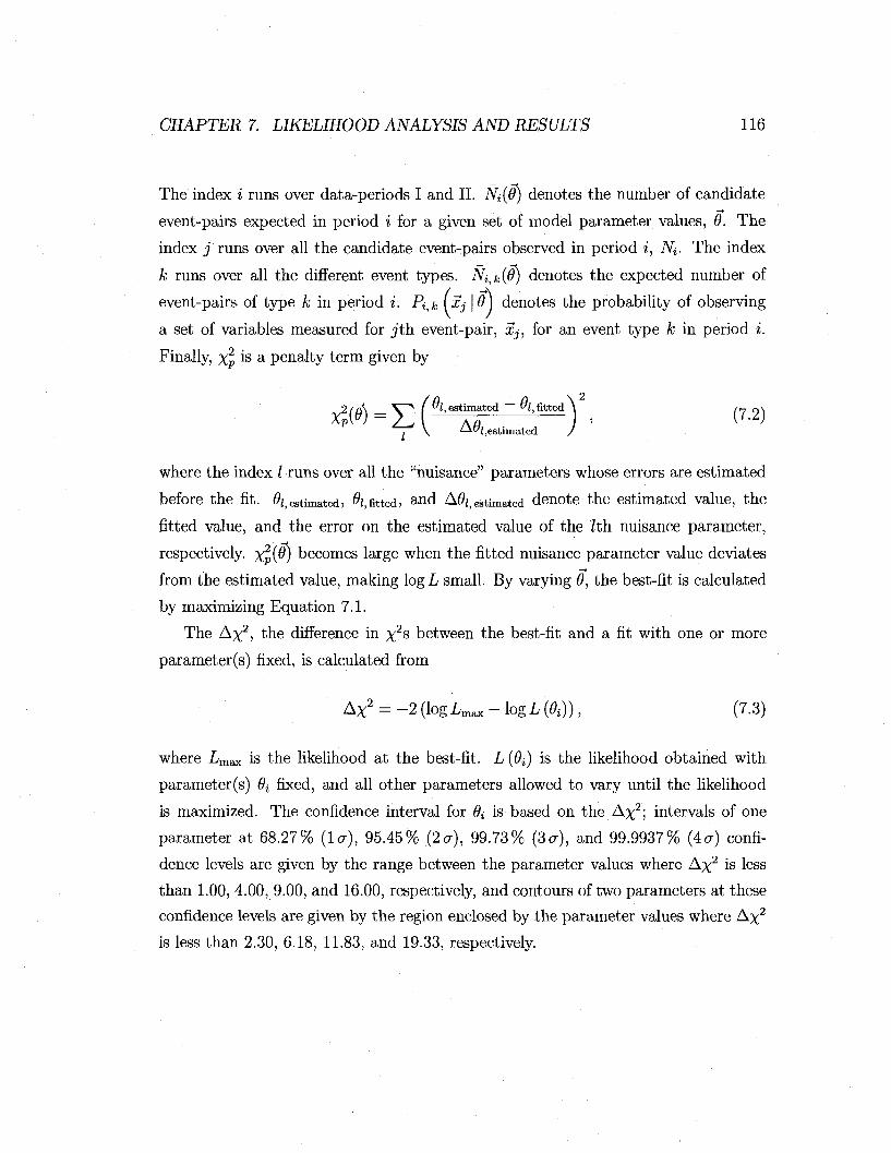
CHAPTER 7. LIKELIHOOD ANALYSIS AND RESULTS 116
The index % runs over data-periods I and II. N0) denotes the number of candidate
event-pairs expected in period i for a given set of model parameter values, 6. The
index j runs over all the candidate event-pairs observed in period i, Nt. The index
k runs over all the different event types. Nitk(v) denotes the expected number of
event-pairs of type k in period i. P^k (xj\6) denotes the probability of observing
a set of variables measured for j th event-pair, Xj, for an event type k in period i.
Finally, %2 is a penalty term given by
2//i\ V ^ / "l, estimated — "l, fitted \ /n 0 \
Xp(e) = 2^ ( - ^ \ f l — ' (7-2) , \ i-it7Z,estimated /
where the index I runs over all the "nuisance" parameters whose errors are estimated
before the fit. fyestimated, fyfitted, and A^jestimated denote the estimated value, the
fitted value, and the error on the estimated value of the lih nuisance parameter,
respectively. x^>iy) becomes large when the fitted nuisance parameter value deviates —*
from the estimated value, making logL small. By varying 8, the best-fit is calculated
by maximizing Equation 7.1.
The A%2, the difference in %2s between the best-fit and a fit with one or more
parameter(s) fixed, is calculated from
Ax2 = - 2 ( l o g L m a x - l o g L ( ^ ) ) , (7.3)
where Lmax is the likelihood at the best-fit. L (0i) is the likelihood obtained with
parameter(s) fy fixed, and all other parameters allowed to vary until the likelihood
is maximized. The confidence interval for 9i is based on the A%2; intervals of one
parameter at 68.27% ( la) , 95.45% (2a), 99.73% (3a), and 99.9937% (4a) confi
dence levels are given by the range between the parameter values where A%2 is less
than 1.00, 4.00, 9.00, and 16.00, respectively, and contours of two parameters at these
confidence levels are given by the region enclosed by the parameter values where A%2
is less than 2.30, 6.18, 11.83, and 19.33, respectively.

CHAPTER 7. LIKELIHOOD ANALYSIS AND RESULTS 117
7.2.1 Mode-I Analysis
ModeJ analysis uses the expected spectra in Ep, Ed, and At for all the expected
event types, i.e., Piik ixj\6\ in Equation 7.1 is given by
7.2.2 Mode-II Analysis
As well as Ep, Ed, and At, Mode-II analysis uses the expected spectra in t, in order
to help discriminating the Preactor signals from all the other event types. Pijk (XJ | 9J
in Equation 7.1 for Mode-II analysis is given by
For PreactorS, this is given by
"•*», reactor (x) |9) =
dEpdEddAtdt rIP / _.\ AP rIP-U,J- i, reactor / -» i n \ ^ «* reactor / -> \ UjX t
( -» I n\ "•*»,reactor / -> \ ™'*i,reactor / -> \ l<-i n\
We)-dRr(Xi)-dzr(Xi)> (7-6) dEpdt \ J I / dEd
while for all other event types it is given by
dPi, k (-> \ n\ 1 dPit k (., , z\ dPit k , _ v dPit k dEpdEddAtdt Kjl J ~ Tt dEv r j l 7 d £ d
{Xj) dAt [Xjh [IJ)
where Tj is the total livetime in period i.
7.2.3 Mode-I l l Analysis
Assuming CPT-invariance, which implies that the ue survival probability is the same
as that of ue for the same energy and baseline, Mode-Ill analysis combines Mode-II
analysis with the flux measurements of the z s from the sun (solar us), performed by
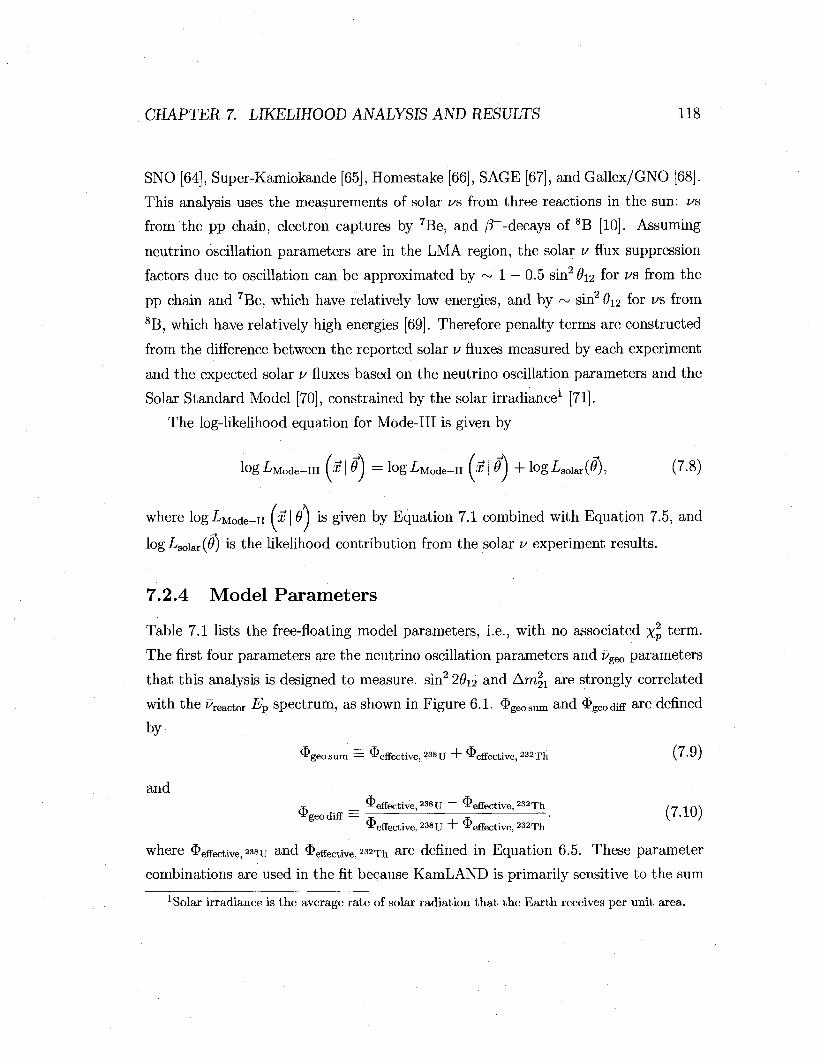
CHAPTER 7. LIKELIHOOD ANALYSIS AND RESULTS 118
SNO [64], Super-Kamiokande [65], Homestake [66], SAGE [67], and Gallex/GNO [68].
This analysis uses the measurements of solar us from three reactions in the sun: us
from the pp chain, electron captures by 7Be, and /?+-decays of 8B [10]. Assuming
neutrino oscillation parameters are in the LMA region, the solar u flux suppression
factors due to oscillation can be approximated by ~ 1 — 0.5 sin2 6u for us from the
pp chain and 7Be, which have relatively low energies, and by ~ sin2 #i2 for z s from 8B, which have relatively high energies [69]. Therefore penalty terms are constructed
from the difference between the reported solar u fluxes measured by each experiment
and the expected solar u fluxes based on the neutrino oscillation parameters and the
Solar Standard Model [70], constrained by the solar irradiance1 [71].
The log-likelihood equation for Mode-Ill is given by
log I/Mode-m [x | 6 J = log LMode-n [x\9j + log Lsoiar($), (7.8)
where logLMode-n (%\ 9) is given by Equation 7.1 combined with Equation 7.5, and
logLso\ar(v) is the likelihood contribution from the solar u experiment results.
7.2.4 Model Parameters
Table 7.1 lists the free-floating model parameters, i.e., with no associated x% term.
The first four parameters are the neutrino oscillation parameters and Pgeo parameters
that this analysis is designed to measure, sin2 2#i2 and Am|x are strongly correlated
with the Reactor Ep spectrum, as shown in Figure 6.1. $geosum and $geodifF are defined
by
"Pgeosum = ^effective, 2 3 8 U ~l~ ^"effective, 2 3 2 Th
(7.9)
and , _ ^effective, 2 3 8 U ~ ^effective, 2 3 2 Th f7in\
$geodiff = ^ — V • (7.1UJ ^effective, 238 u + ^effective, 232 T h
where Effective, 238u and effective, 232Th are defined in Equation 6.5. These parameter
combinations are used in the fit because KamLAND is primarily sensitive to the sum 1 Solar irradiance is the average rate of solar radiation tha t the Ear th receives per unit area.
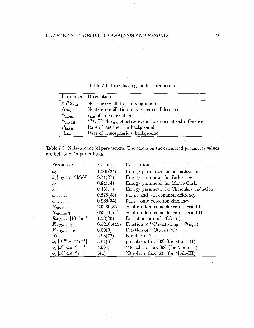
CHAPTER 7. LIKELIHOOD ANALYSIS AND RESULTS 119
Table 7.1: Free-floating model parameters.
Parameter
sin2 2612
Am|i
^*geo sum
™geo difF
-rtfastn
" a t m t '
Description
Neutrino oscillation mixing angle Neutrino oscillation mass-squared difference ugeo effective event rate 2 3 8 u _ 2 3 2 T n
i geo effective event rate normalized difference Rate of fast neutron background Rate of atmospheric v background
Table 7.2: Nuisance model parameters. The errors on the estimated parameter values are indicated in parentheses.
Parameter
a0
^ [ m g c m ^ M e V - 1 ] k0
kc
^•common
^reactor
• ' random I
-^random II
^ c ^ t l O - S - 1 ] ^ 1 3 C ( a , n ) , C
,n) 1 6 0*
AT 9 L i
^ [ l O ^ c m ^ s - 1 ] ^ [ l O ^ m ^ s - 1 ] <j)8 [106 cm"2 s"1]
Estimate
1.061(24) 9.71(27) 0.84(14) 0.43(11) 0.875(35) 0.986(34) 202.30(35) 653.41(74) 1.53(20) 0.02105(45) 0.09(9) 2.98(72) 5.94(6) 4.9(6) 6(1)
Description
Energy parameter for normalization Energy parameter for Birk's law Energy parameter for Monte Carlo Energy parameter for Cherenkov radiation reactor and ugeo common efficiency reactor only detection efficiency
# of random coincidence in period I # of random coincidence in period II Detection rate of 13C(a, n) Fraction of 12C scattering 1 3C(a, n) Fraction of 1 3C(a,n) 1 60* Number of 9Li pp solar v flux [63] (for Mode-Ill) 7Be solar v flux [63] (for Mode-Ill) 8B solar v flux [63] (for Mode-Ill)

CHAPTER 7. LIKELIHOOD ANALYSIS AND RESULTS 120
of the 238U and 232Th ugeo fluxes, rather than their difference, for which the geochem-
ical measurements of meteorites and rocks have better sensitivity (see Section 1.3.2).
The reference Earth model described in Section 1.3.2, predicts the central values of
geosum and $geodiff to be 61 (1032p • yr)_1 and 0.6, respectively. If the Earth is "fully
radiogenic," as described in Section 6.2, <&geosum can take a range between 98 and 142
(HFp-yr ) - 1 .
The rate of fast neutron and atmospheric v backgrounds, i?fastn and Ratmv in
Table 7.1, respectively, are difficult to estimate, and hence they are freely floated
in this analysis. The ue candidate prompt events at high Ep can discriminate these
backgrounds from other types of events since no other event types are expected above
~10 MeV except the 9Li backgrounds, whose expected number of event-pairs in the
data-set is estimated fairly accurately.
Table 7.2 lists the model nuisance parameters. The four energy parameters dis
cussed in Section 3.4 modify the expected Ep PDF shapes for factor and ugeo signals
and 13C(a, n) and 9Li backgrounds. Since the error on eseo is negligible compared to
the statistical error on the geosumj £geo is not fitted. Based on the spectral shape, 6EP
for these event types are calculated during the fit. </>i, 07, and (f)S are the expected
solar flux at the surface of the Earth in the absence of neutrino oscillation, described
in Section 7.2.3.
7.3 Best-Fits
The unbinned maximum log-likelihood fits from Mode-I, II, and III analyses determine
the best-fit model parameter values as summarized in Table 7.3. This shows that none
of the best-fit nuisance model parameters deviates from the estimated values. Fig
ures 7.2 and 7.3, for Mode-I and II analyses, respectively, show the best-fit Ep spectra
of various event types as well as the distributions of the candidates after subtracting
the best-fit random coincidence background. The random coincidence background Ep
spectrum is easily subtracted since it is directly measured, unlike many of the other
spectra which are calculated based on the theoretical Erea\ and energy parameters.
The top plots show the entire Ev region analyzed, and the middle and bottom plots
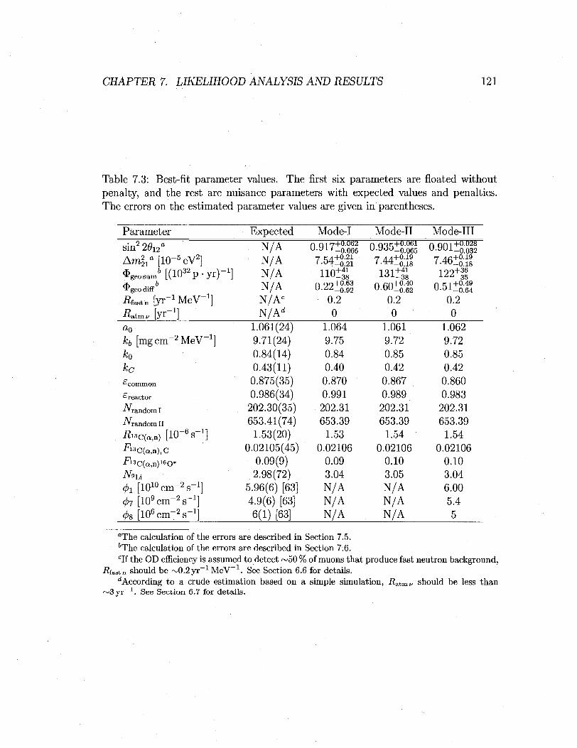
CHAPTER 7. LIKELIHOOD ANALYSIS AND RESULTS 121
Table 7.3: Best-fit parameter values. The first six parameters are floated without penalty, and the rest are nuisance parameters with expected values and penalties. The errors on the estimated parameter values are given in parentheses.
Parameter Expected Mode-I Mode-II Mode-Ill sin2 2612
a
Am^a[10-5eV2] ^ g e o s u m M a O ^ P - y r ) - 1 ]
^•geodiff
tffastntyr^MeV"1] # a w [yr-1] a0
kb [mgcm~2MeV_1] k0
kc
^common
^reactor
•* "randomI
-'•random II
RuC(a,n) [lO-'V1] ^ 1 3 C ( a , n ) , C
F13C(a,n)160* N*u ^i [UPcm^s-1] ^ K c m ^ s ' 1 ] (j)8 [l(fi CUT2 8'1]
N/A N/A N/A N/A N/Ac
N/Ad
1.061(24) 9.71(24) 0.84(14) 0.43(11) 0.875(35) 0.986(34) 202.30(35) 653.41(74)
1.53(20) 0.02105(45)
0.09(9) 2.98(72)
5.96(6) [63] 4.9(6) [63] 6(1) [63]
n Q17+u-oea u - y i ' - 0 . 0 6 6
7.541SS "OlS
rv 99+0.63 u - z z - 0 . 9 2
0.2 0
1.064 9.75 0.84 0.40 0.870 0.991 202.31 653.39
1.53 0.02106
0.09 3.04 N/A N/A N/A
n QQK+o-oei u.yod_0065
7.4ns 1311S
0 60+a4° U - O U - 0 . 6 2 0.2
0 1.061 9.72 0.85 0.42
0.867 0.989 202.31 653.39
1.54 0.02106
0.10 3.05 N/A N/A N/A
u.yui_o.o32
7.4612:2 122+H
U - O i - 0 . 6 4
0.2 0
1.062 9.72 0.85 0.42 0.860 0.983 202.31 653.39
1.54 0.02106
0.10 3.04 6.00 5.4 5
aThe calculation of the errors are described in Section 7.5. 6The calculation of the errors are described in Section 7.6. cIf the OD efficiency is assumed to detect ~50 % of muons that produce fast neutron background,
-Rfastn should be ~0.2yr_ 1 MeV . See Section 6.6 for details. d According to a crude estimation based on a simple simulation, i?atIIU, should be less than
~3yT~:l. See Section 6.7 for details.

CHAPTER 7. LIKELIHOOD ANALYSIS AND RESULTS 122
a 102
10
z
/ - • •y^^fe^- lK^* " ^ ^ V .
4^m
m y///K\ '• \ \ '• \ ////A \ ' \ ' ' X ^ S ^
/ / / / / \ * l l • i i \ ^ ^
All combined All except Vgeo
V reactor
^ 2 3 2 T h 7 g e o
— - > , n ) 9Li Fast n
vyyy\ N> •' ' ' ' \ ~~" V///4A: . 1 . . . i l l . . '.. i . \ ' . - - v . i . . . i . . i .
12 14 Ep [MeV]
I
9 10 Ep [MeV]
400
Ep [MeV]
Figure 7.2: Mode-I analysis best-fit .Ep spectra. The dots with error bars are candidate event distribution minus best-fit random coincidence background spectrum. The spectra shown are all combined, all combined except useo, £>reactor, 238U uFen,
232rph geo, 13C(a, n), 9Li, and fast neutrons; see the legend in the top plot.
geoj
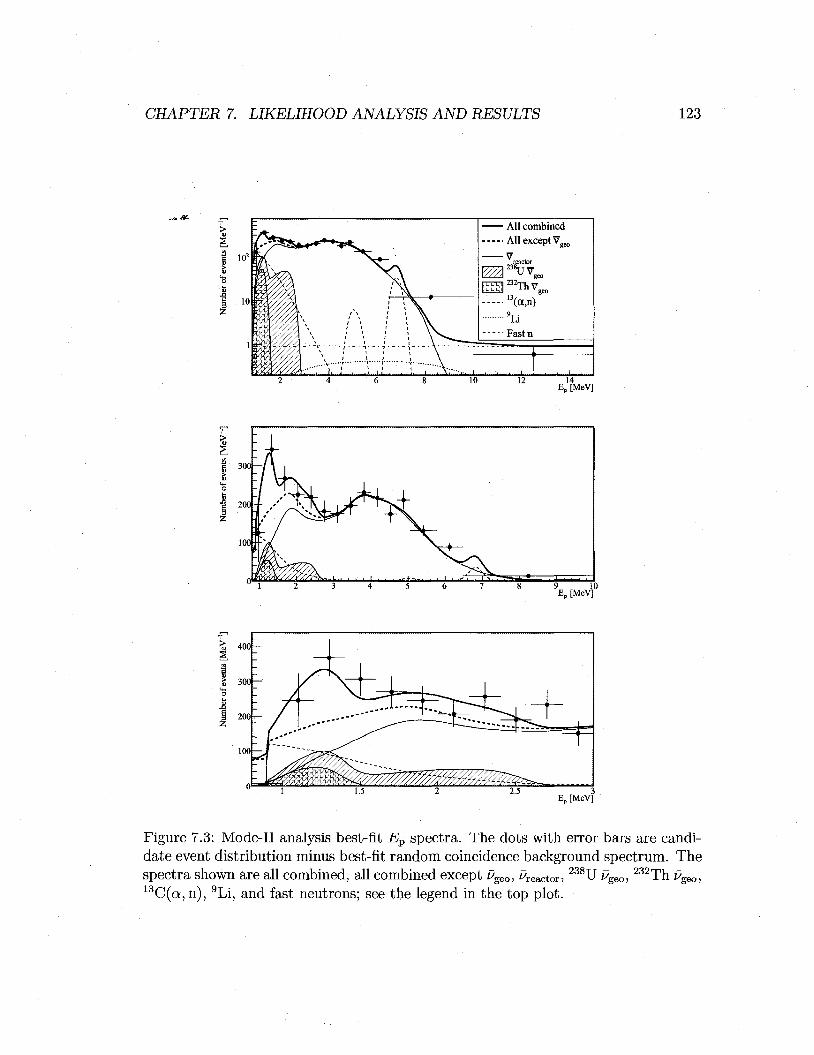
CHAPTER 7. LIKELIHOOD ANALYSIS AND RESULTS 123
o2
10
~h*' ^ S * ^ * i * ' * y <
/////A V t i i
^yLA/CA _ . _%. _ . „ . 7 _ j . _ . 7 . _ . _
All combined All except vgeo
v" , reactor
^ 2 3 8 u v g e o
— - > , n ) 9Li Fast n
10 14 Ep [MeV]
I 3
400
Ep [MeV]
Figure 7.3: Mode-II analysis best-fit Ep spectra. The dots with error bars are candidate event distribution minus best-fit random coincidence background spectrum. The spectra shown are all combined, all combined except vgeo, Reactor, 238U Pgeo,
232Th Pgeo, 13C(a,n), 9Li, and fast neutrons; see the legend in the top plot.
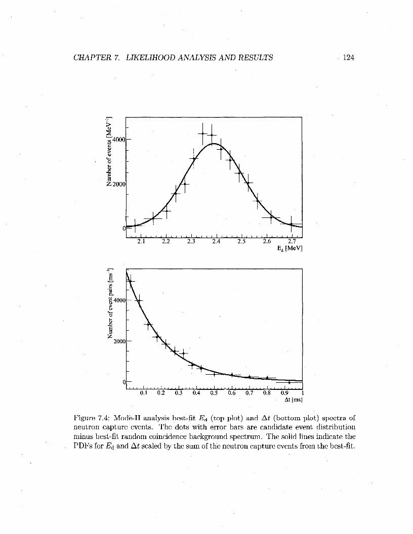
CHAPTER 7. LIKELIHOOD ANALYSIS AND RESULTS 124
>
,4000 el
>
O
&
£2000
Oh • • • t I I I I I 1 I I I I I . I I I I I I I I I I I I I I I I I I I I I I I I I I I I I I I I I
0.1 0.2 0.3 0.4 0.5 0.6 0.7 0.8 0.9 1 At [ms]
Figure 7.4: Mode-II analysis best-fit Ed (top plot) and At (bottom plot) spectra of neutron capture events. The dots with error bars are candidate event distribution minus best-fit random coincidence background spectrum. The solid lines indicate the PDFs for Ed and At scaled by the sum of the neutron capture events from the best-fit.

CHAPTER 7. LIKELIHOOD ANALYSIS AND RESULTS 125
xl(T
1000 1200 1400 1600 1800 Days since April .3, 2002 [days]
Figure 7.5: Mode-II analysis best-fit time spectra. The dots with error bars are candidate event-pair distribution minus best-fit random coincidence background spectrum. The thin solid line indicates the best-fit Reactor spectrum. The dotted line indicates the sum of the best-fit spectra for ugeo signal and 13C(a,n), 9Li, fast neutron, and atmospheric v backgrounds. The thick solid line is the sum of the spectra indicated by the dotted and thin solid lines.

CHAPTER 7. LIKELIHOOD ANALYSIS AND RESULTS 126
focus on the factor a n d t'geo Ep regions, respectively. The main differences between
the best-fit Ep spectra from Mode-I and II analyses are the normalizations of 238U and 232Th ugeos. The top and bottom plots in Figure 7.4 and Figure 7.5 show the best-fit
E<x, At, and t spectra from Mode-II analysis, respectively, all obtained by combining
the best-fit spectra of all the event types, except random coincidence backgrounds.
These plots also show the distributions of the candidate event-pairs after subtracting
the best-fit random coincidence backgrounds spectra. The best-fit E& and At spectra
from Mode-I are not appreciably different from those from Mode-II analysis. The
correlation coefficient matrices for Mode-I, II, and III analysis best-fits are given in
Tables 1.1, 1.2, and 1.3, respectively, in Appendix I.
7.4 Goodness-of-Fit
Based on how well a particular model fits the data, "goodness-of-fit," the model can
be accepted or rejected. Although the unbinned maximum likelihood fit effectively
determines the best-fit parameter values, x2 = ~2 log L at its maximum does not yield
the goodness of the fit to the data [72]. Instead, the goodness-of-fit for Mode-I analysis
is estimated using a Monte Carlo simulation from the following procedures. First,
1000 Monte Carlo data-sets are created using the best-fit Ep, E& and At spectra of
all event types from Mode-I analysis. The number of each event type to be simulated
in each Monte Carlo data-set is obtained from a Poisson distribution with a mean
from the best-fit number of events of the actual candidate data-set. Using the exact
same method as the real data-set, all the parameters are fitted for each Monte Carlo
data-set. Using the resulting best-fit spectra, equal-probability-binning histograms
are prepared for the Ep, E& and At distributions, and the Pearson %2 for each variable
is calculated for each data-set. As an example, the top plot in Figure 7.6 shows the Ep
distribution of the actual candidate data-set in 50 equal-probablity binning, used to
calculate the Pearson x2- F ° r a given number of bins, the Pearson x2 of the candidate
data-set is compared to those of the Monte Carlo data-sets. The goodness-of-fit p-
value is the fraction of Monte Carlo data-sets that have a Pearson %2 larger than that
of the candidate data-set. As examples, Figure 7.7 shows the Pearson x2 distributions

CHAPTER 7. LIKELIHOOD ANALYSIS AND RESULTS 127
.a "§ I >
10 Ep [MeV]
I >
Figure 7.6: Ep distributions of candidates (markers with error bars) in 50 equal-probablity bins, prepared from the best-fit Ep spectra (solid lines). Top plot is for the best-fit obtained assuming two-flavor neutrino oscillation. The bottom plot is for the best-fit obtained assuming no neutrino oscillation and floating ereactor without a penalty, as described in Section 7.4.1.

CHAPTER 7. LIKELIHOOD ANALYSIS AND RESULTS 128
.a loo.
.glOO
a 80-
60
40
20
Figure 7.7: Pearson %2 distributions for 50 equal-probablity binnings of the Monte Carlo Ep (top plot), Ed (middle plot), and At (bottom plot) distributions. The vertical dotted lines indicate the Pearson %2 for the candidate data-set.

CHAPTER 7. LIKELIHOOD ANALYSIS AND RESULTS 129
a. « 0.8|
0.6f—
0.2—
M I
r i i
I T I * ^ i
* i * T I
I I I 1 I I I J
- 1 — - J - 1 . . . . J . . . ••!•••
'10 20 60 70 Number of bins
6 0-8H
* o.a—
0.4
0.2K
I I
^ z 1 1 z xi ^
i ' i
i l i i i
i i . i
'10 20 30 40 50 60 70 Number of bins
2 1
S 0.8
0.4
0.21—
i i i i
I I :
I I I I
'10 20 30 40 50 60 70 Number of bins
Figure 7.8: Ep (top plot), Ed (middle plot), At (bottom plot) spectra goodness-of-fit p-value vs. number of equal-probablity bins. The uncertainties in the goodness-of-fit p-value due to the statistical errors of the Monte Carlo simulation are shown as the error bars.
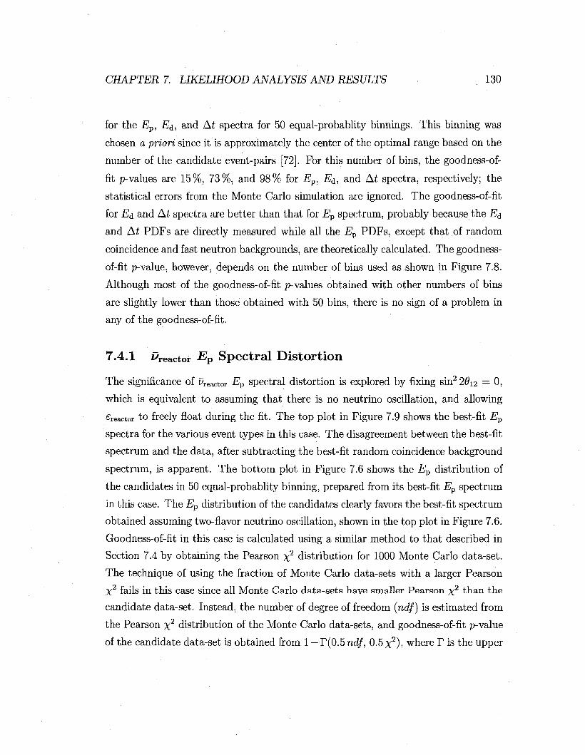
CHAPTER 7. LIKELIHOOD ANALYSIS AND RESULTS 130
for the Ep, Ed, and At spectra for 50 equal-probablity binnings. This binning was
chosen a priori since it is approximately the center of the optimal range based on the
number of the candidate event-pairs [72]. For this number of bins, the goodness-of-
fit p-values are 15%, 73%, and 98% for Ep, E&, and At spectra, respectively; the
statistical errors from the Monte Carlo simulation are ignored. The goodness-of-fit
for Ed and At spectra are better than that for Ep spectrum, probably because the E&
and At PDFs are directly measured while all the Ep PDFs, except that of random
coincidence and fast neutron backgrounds, are theoretically calculated. The goodness-
of-fit p-value, however, depends on the number of bins used as shown in Figure 7.8.
Although most of the goodness-of-fit p-values obtained with other numbers of bins
are slightly lower than those obtained with 50 bins, there is no sign of a problem in
any of the goodness-of-fit.
7.4.1 Reactor ^ p Spectral Distortion
The significance of Reactor Ep spectral distortion is explored by fixing sin2 2#i2 = 0,
which is equivalent to assuming that there is no neutrino oscillation, and allowing
Reactor to freely float during the fit. The top plot in Figure 7.9 shows the best-fit Ep
spectra for the various event types in this case. The disagreement between the best-fit
spectrum and the data, after subtracting the best-fit random coincidence background
spectrum, is apparent. The bottom plot in Figure 7.6 shows the Ep distribution of
the candidates in 50 equal-probablity binning, prepared from its best-fit Ep spectrum
in this case. The Ep distribution of the candidates clearly favors the best-fit spectrum
obtained assuming two-flavor neutrino oscillation, shown in the top plot in Figure 7.6.
Goodness-of-fit in this case is calculated using a similar method to that described in
Section 7.4 by obtaining the Pearson x2 distribution for 1000 Monte Carlo data-set.
The technique of using the fraction of Monte Carlo data-sets with a larger Pearson
X2 fails in this case since all Monte Carlo data-sets have smaller Pearson x2 than the
candidate data-set. Instead, the number of degree of freedom (ndf) is estimated from
the Pearson x2 distribution of the Monte Carlo data-sets, and goodness-of-fit p-value
of the candidate data-set is obtained from 1 — T(0.5 ndf, 0.5 x2), where T is the upper

CHAPTER 7. LIKELIHOOD ANALYSIS AND RESULTS 131
fc All combined All except vgeo
'Uv„ reactor
I 238
9 10 Ep [MeV]
>
^ i o - 3
•I Jio-4
io-
10"'
1 1 I
I I I
1 I I I I 1
1 I ' I I 1
1 I II I I l
I I I I I I
I I , I
I I I I
M • ' I I I ' J i I I L _
10 20 30 40 50 60 70 Number of bins
Figure 7.9: Best-fit Ep spectra (top plot) and goodness-of-fit p-values (bottom plot) obtained using unoscillated Cwtor spectrum with unconstrained normalization. Top plot: the best-fit random coincidence events are subtracted from the data (markers with error bars). The best-fit Ep spectra of fast neutron, 9Li, and atmospheric v backgrounds are too small to be seen. Bottom plot: the goodness-of-fit p-value depends on the number of equal-probablity bins. The uncertainties in the goodness-of-fit p-value due to the statistical errors of the Monte Carlo simulation are shown as the error bars.
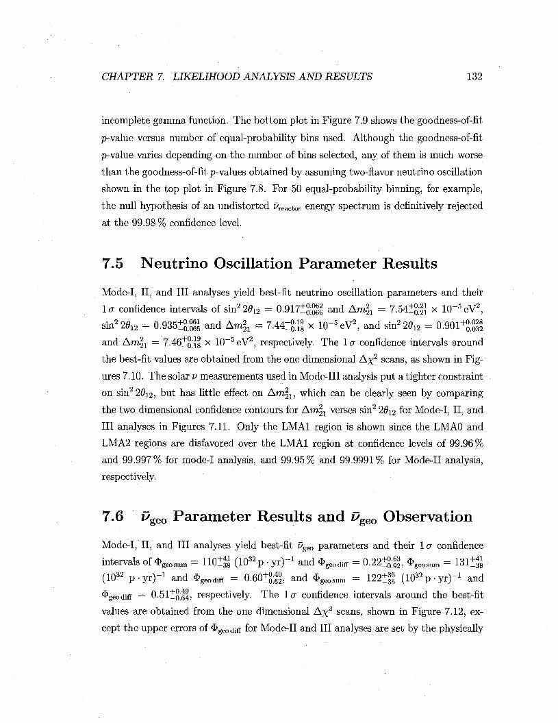
CHAPTER 7. LIKELIHOOD ANALYSIS AND RESULTS 132
incomplete gamma function. The bottom plot in Figure 7.9 shows the goodness-of-fit
p-value versus number of equal-probability bins used. Although the goodness-of-fit
p-value varies depending on the number of bins selected, any of them is much worse
than the goodness-of-fit p-values obtained by assuming two-flavor neutrino oscillation
shown in the top plot in Figure 7.8. For 50 equal-probability binning, for example,
the null hypothesis of an undistorted Reactor energy spectrum is definitively rejected
at the 99.98 % confidence level.
7.5 Neutr ino Oscillation Parameter Results
Mode-I, II, and III analyses yield best-fit neutrino oscillation parameters and their
lcr confidence intervals of sin22012 = 0.917tao66 a n d A™!i = 7.54±S:ii x 10"5eV2,
sin22012 = 0.935i{j;gj& and Am?21 = 7.44±g;Jl x l(T5eV2, and sin22012 = 0.901^32
and Amli = 7.46±g;Jl x 10 5eV2, respectively. The la confidence intervals around
the best-fit values are obtained from the one dimensional A^2 scans, as shown in Fig
ures 7.10. The solar u measurements used in Mode-Ill analysis put a tighter constraint
on sin22#12, but has little effect on Am^, which can be clearly seen by comparing
the two dimensional confidence contours for Ara21 verses sin2 2#i2 for Mode-I, II, and
III analyses in Figures 7.11. Only the LMAl region is shown since the LMA0 and
LMA2 regions are disfavored over the LMAl region at confidence levels of 99.96%
and 99.997% for mode-I analysis, and 99.95% and 99.9991 % for Mode-II analysis,
respectively.
7.6 £/geo Parameter Results and Pgeo Observation
Mode-I, II, and III analyses yield best-fit ugeo parameters and their 1 a confidence
intervals of $geosum = 110±|| (1032p • yr)"1 and $geodifF = 0.22t°;<>3, $geosum = 131±||
(1032 p -y r ) - 1 and $geodiff = 0.6018$, and $geogum = 122±! ( lO^p-yr)"1 and
• geodiff = 0.5liQ;g4, respectively. The 1 a confidence intervals around the best-fit
values are obtained from the one dimensional A%2 scans, shown in Figure 7.12, ex
cept the upper errors of <frgeodiff for Mode-II and III analyses are set by the physically
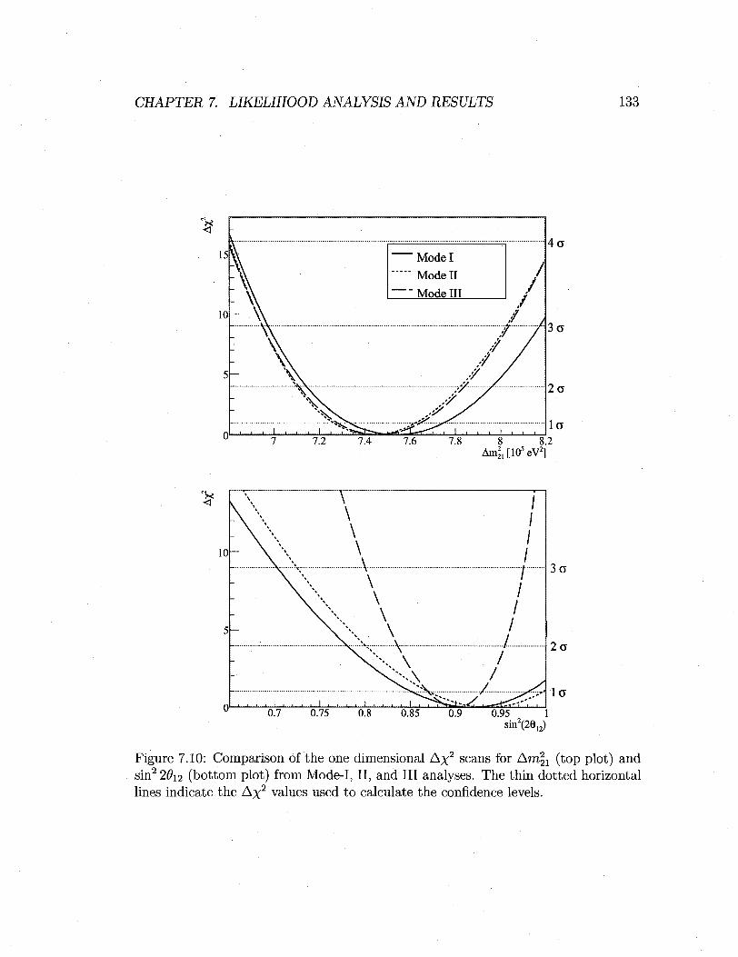
CHAPTER 7. LIKELIHOOD ANALYSIS AND RESULTS 133
Am^[105eV2;
Figure 7.10: Comparison of the one dimensional A%2 scans for Am^ (top plot) and sin2 20i2 (bottom plot) from Mode-I, II, and III analyses. The thin dotted horizontal lines indicate the A%2 values used to calculate the confidence levels.

CHAPTER 7. LIKELIHOOD ANALYSIS AND RESULTS 134
T 7.5
• ' ' ' • —'.r..:.r.*. j . j .J...... i I • i__j i L . . . I — - J — i 1 i i
0.65 0.7 0.8 0.85 0.9 0.95 , 1 sin2(2612)
7.5 —
0.65 0.75 0.85
_
-
i i i._i L „ I ' T I
-
*-*
\ V •
- • 1 . • • • 1 . - i - . l
0.9 0.95 , 1 sin2(2012)
f
CO) - I — I — I — I — I • — ' • • * • • • • J ' *• I
0.65 0.7 0.75 0.8 0.85 0.9 0.95 , 1 sin2(2612)
Figure 7.11: Neutrino oscillation parameter confidence contours for Mode-I (top plot), II (middle plot), and III (bottom plot) analyses. The confidence levels are 1 a (solid), 2cr (dashed), 3a (dotted), and 4er (dot-dashed). The dots indicate the best-fit values.
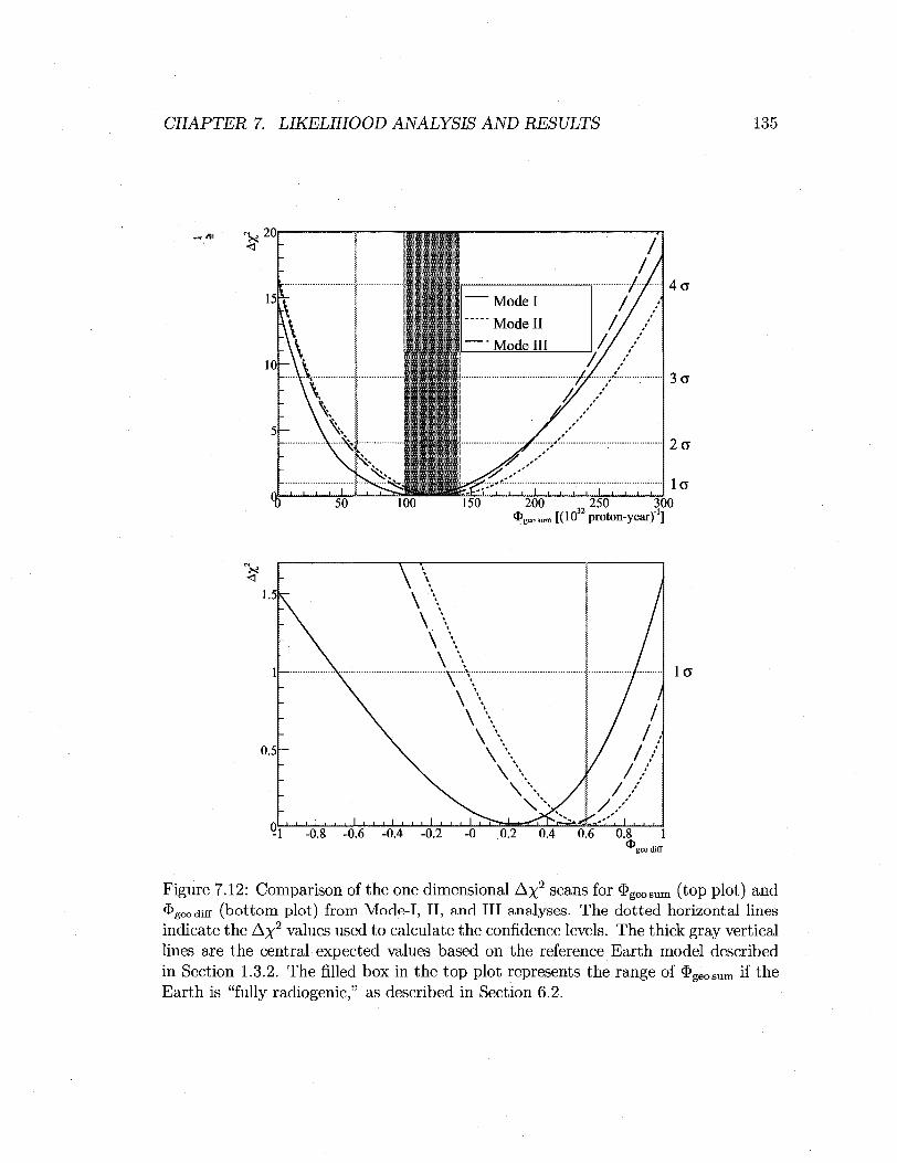
CHAPTER 7. LIKELIHOOD ANALYSIS AND RESULTS 135
4CT
3o
2a
l a 50 100 150 200 " M 2 5 0 " ~ 300
•SgeosmnlXlO proton-year)"1]
Figure 7.12: Comparison of the one dimensional A%2 scans for $geosum (top plot) and ^geodiff (bo t tom plot) from Mode-I, II, and III analyses. The dot ted horizontal lines indicate the A%2 values used to calculate the confidence levels. The thick gray vertical lines are the central expected values based on the reference Earth model described in Section 1.3.2. The filled box in the top plot represents the range of $geogum if the Earth is "fully radiogenic," as described in Section 6.2.

CHAPTER 7. LIKELIHOOD ANALYSIS AND RESULTS 136
J T - 3 0 0
200 —
100
- • - ' • " " " '
•C-H 300i
Figure 7.13: Pgeo parameter confidence contours for Mode-I (top plot), II (middle plot), and III (bottom plot). The confidence levels are la (solid), 2cr (dashed), 3cr (dotted), and 4cr (dot-dashed). The black circular markers indicate the best-fit values. The gray triangular markers indicate the central predicted value based on the reference Earth model described in Section 1.3.2. The gray line segments represent the range of $ge0sum if the Earth is "fully radiogenic," as described in Section 6.2.
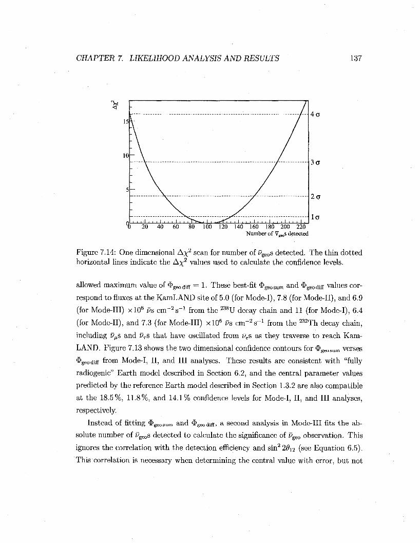
CHAPTER 7. LIKELIHOOD ANALYSIS AND RESULTS 137
4a
3a
2a
la t) 20 40 60 80 100 120 140 160 180 200 220
Number of vgeos detected
Figure 7.14: One dimensional Ax2 scan for number of vgeos detected. The thin dotted horizontal lines indicate the A%2 values used to calculate the confidence levels.
allowed maximum value of $geodiflf = 1- These best-fit $geosum and $geodiff values cor
respond to fluxes at the KamLAND site of 5.0 (for Mode-I), 7.8 (for Mode-II), and 6.9
(for Mode-Ill) xlO6 us cm~ 2 s _ 1 from the 238U decay chain and 11 (for Mode-I), 6.4
(for Mode-II), and 7.3 (for Mode-Ill) xlO6 i s c r n ^ s " 1 from the 232Th decay chain,
including z^s and 9Ts that have oscillated from ves as they traverse to reach Kam
LAND. Figure 7.13 shows the two dimensional confidence contours for $ g e o s u m verses
^geodiff from Mode-I, II, and III analyses. These results are consistent with "fully
radiogenic" Earth model described in Section 6.2, and the central parameter values
predicted by the reference Earth model described in Section 1.3.2 are also compatible
at the 18.5%, 11.8%, and 14.1% confidence levels for Mode-I, II, and III analyses,
respectively.
Instead of fitting $ g e o s n m and <frgeodiff, a second analysis in Mode-Ill fits the ab
solute number of ugeos detected to calculate the significance of Pgeo observation. This
ignores the correlation with the detection efficiency and sin2 2#X2 (see Equation 6.5).
This correlation is necessary when determining the central value with error, but not
1 *
CHAPTER 7. LIKELIHOOD ANALYSIS AND RESULTS 138
necessary when only testing whether observed. Figure 7.14 shows the one
dimensional A%2 scan for the number of Pgeos detected. The observation of ^geos is
confirmed at the 99.995 % confidence level.
7.7 Nuclear Reactor at the Center of the Earth
A rather controversial Earth model is proposed, which suggests the existance of a
"georeactor," a naturally occurring nuclear reactor, fueled by uranium, at the very
center of the Earth's core [73, 74]. This hypothesis conflicts with the widely accepted
Earth model that uranium concentration in the iron core is negligible since uranium
is chemically incompatible with iron (see Section 1.3.2). However, from a strictly
empirical point of view, this hypothesis is difficult to refute using existing geological
and geophysical data. If a georeactor existed, it would produce z/es, which could be
detected with KamLAND. According to the model [73, 74], the georeactor produces
up to approximately 10 TW of thermal power from nuclear fission of 235U and 238U,
which comprise 76 % and 24 % of the georeactor fission, respectively. The expected
Ep spectral shape is the weighted sum of the spectra of z?es from /^-decays of fragments
following 235U and 238U fission, shown in Figure 1.7, which is then converted into a
Evis spectrum. The expected georeactor ue detection rate, given per target proton
per unit time can be expressed as
georeactor = E ^ ^ J P ^ ( ^ , R*) a(EpJ J ^ P J dE*., (7 .11)
where e is the detection efficiency, /georeactor denotes the fission rate in the georeactor,
R® denotes the radius of the Earth, PPe^Pe(EPe, Re) denotes the De survival proba
bility due to neutrino oscillation (see Equation 1.5), a denotes the inverse /?-decay
cross-section (see Figure 1.6), and -^r- denotes the energy spectrum of the produced
Pes given in number of &es per fission per unit energy. Since i?© is much larger than
Epe/Am2i, the sin2 I m^_ e J term in the survival probability (see Equation 1.5) re
sults in many oscillations in the 9e energy spectrum. However, an oscillation pattern
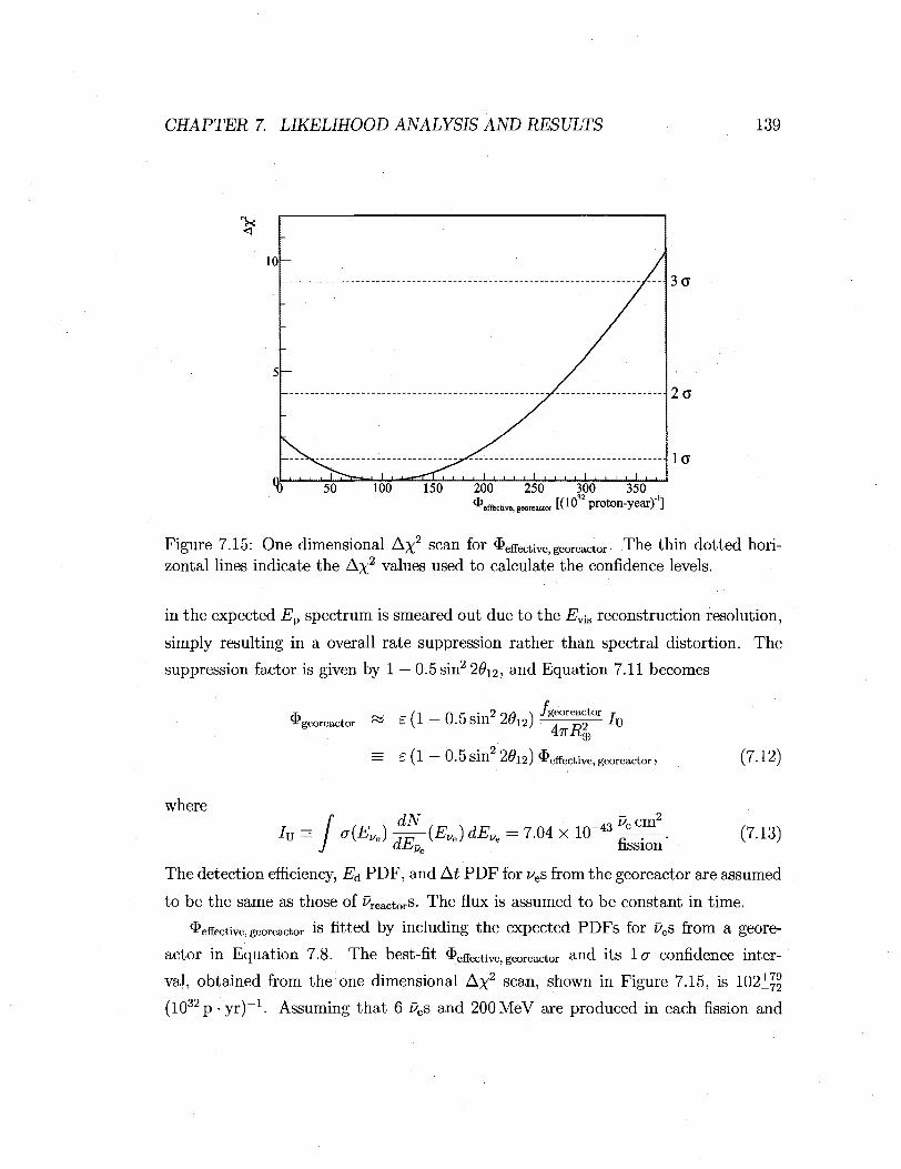
CHAPTER 7. LIKELIHOOD ANALYSIS AND RESULTS 139
$
200 effective, georeactoi
250 300 350 ir [(10 proton-year)"1]
Figure 7.15: One dimensional A%2 scan for " effective, georeactor- The thin dotted horizontal lines indicate the A%2 values used to calculate the confidence levels.
in the expected Ep spectrum is smeared out due to the Evis reconstruction resolution,
simply resulting in a overall rate suppression rather than spectral distortion. The
suppression factor is given by 1 — 0.5 sin2 2012, and Equation 7.11 becomes
$ georeactor ~ £ (1 ~~ 0.5 s in 2#12) — — ^ — I \ J
= £ ( 1 — 0.5 Sin 2^i2j "^effective,georeactor, (7.12)
where h s / °(E-] ^}E-)dE- -7M x 10_43 £ s £ <n3>
The detection efficiency, E& PDF, and At PDF for ves from the georeactor are assumed
to be the same as those of Reactors. The flux is assumed to be constant in time.
effective, georeactor is fitted by including the expected PDFs for Pes from a geore
actor in Equation 7.8. The best-fit effective,georeactor and its la confidence inter
val, obtained from the one dimensional A%2 scan, shown in Figure 7.15, is 102+™
(1032p • yr)_1. Assuming that 6 Pes and 200 MeV are produced in each fission and

CHAPTER 7. LIKELIHOOD ANALYSIS AND RESULTS 140
Table 7.4: Best-fit parameter value comparison for Mode-Ill analysis with and without georeactor. The errors on the estimated parameter values are given in parentheses.
Parameter Estimate With georeactor
Without georeactor
^effective, georeactor
[(lO^p-yr)-1] sin2 26>i2 A m | [10-5eV2] • S g e o s u m K l O ^ p - y r ) - 1 ]
^geodiff
iZfastntyr^MeV-1] -Ratm i/ [yr-1] a0
kb [mgcm^MeV -1] kQ
kc
^•common
^reactor
^"random I
•L "random II
R™C(a,n) [lO"^-1] Fl3C(a,n),C
Fl3C(a,n)lf>0*
N9Li
fa [ lO^cm^s-1] fa [10° cm"2 a"1] fa l O 6 ™ - ^ " 1
N/A N/A N/A N/A N/A N/A N/A
1.061(24) 9.71(27) 0.84(14) 0.43(11) 0.875(35) 0.986(34) 202.30(35) 653.41(74)
1.53(20) 0.02105(45)
0.09(9) 2.98(72) 5.94(6) 4.9(6) 6(1)
102 0.916 7.50 116 0.31 0.2 0
1.063 9.74 0.84 0.41 0.837 0.963 202.31 653.39
1.54 0.02106
0.09 3.03 5.99 5.5 5
N/A n o n 1+0028 U . y u i -0.032
7.46JSH 122+H
0 P;I+049
U - O i - 0 . 6 4 0.2 0
1.061 9.72 0.85 0.42 0.860 0.983 202.31 653.39
1.54 0.02106
0.10 3.04 6.00 5.4 5

CHAPTER 7. LIKELIHOOD ANALYSIS AND RESULTS 141
its subsequent decays, and taking j?e = 6400 km, the best-fit effective, georeactor corre
sponds to /georeactor = 2.4 x 10²³ fission per second, or a georeactor power generation
of re^rw. However, this result is also consistent with the absence of the georeac
tor at the 15 % confidence level. Table 7.4 summarizes the best-fit values of all the
parameters, none of which changes significantly by the inclusion of the georeactor
contribution. The correlation coefficient matrix for this best-fit is given in Table 1.4
in Appendix I.

CHAPTER 7. LIKELIHOOD ANALYSIS AND RESULTS 142

Chapter 8
Conclusions
Based on data acquired with KamLAND from April 2002 to April 2007, correspond
ing to a 1.8 x 1032 proton-year exposure to ues, the neutrino oscillation parame
ters, sin22#12 and Am^, are determined using ves originating from nuclear reactors
( reactors), and the flux of ues originating from the Earth (Pgeos) are measured. The
Pes are detected via inverse /?-decay, which produces a positron and a neutron. After
selecting candidate prompt-delayed event-pairs and setting up probability distribu
tion functions for the signals and backgrounds, likelihood functions are constructed to
extract the signals, making best use of all information available. The analysis is con
ducted in three modes; Mode-I analysis uses the spectral shapes for the prompt and
delayed event energies (Ep and Ed, respectively), and the time between the prompt
and delayed events (At), Mode-II analysis additionally uses the spectral shape in
absolute time, and Mode-Ill analysis combines Mode-II analysis with solar v experi
mental results assuming CPT-invariance.
Mode-I analysis shows that the Ep distribution of the selected ue candidates is
inconsistent with the spectral shape expected from unoscillated ues at 99.98 % confi
dence level. Rather, the Ep, Ed, and At distributions are more consistent with the
spectral shapes expected from a two-flavor neutrino oscillation; the goodness-of-fit
p-values of the spectra in Ep, Ed, and At are 15 %, 73 %, and 98 %, respectively, indi
cating generally good fit. Mode-II analysis yields best-fit neutrino oscillation param
eters to KamLAND data of sin22012 = 0.935±g;gg and Am^ = 7A4±°0f8 x lQ-5eV2.
143
CHAPTER 8. CONCLUSIONS 144
The estimated A m ^ is slightly lower than the previous result from the KamLAND
collaboration, A m ^ = 7.9lo!5 x 10"5eV2 [44]. The error on A m ^ improved signifi
cantly due to much larger exposure, extension of the analyzed energy range down to
the inverse /?-decay threshold, and better overall control of systematics. In Mode-II
analysis, the so-called LMAO and LMA2 parameter regions are now disfavored over
LMAl region at the 99.95 % and 99.9991 % confidence levels, respectively.
Assuming CPT-invariance, Mode-Ill analysis combines the result obtained with
Mode-II analysis with the results from the solar v experiments, which provides tighter
constraint on sin22#i2, yielding sin22012 = 0 .9011^1 and A m ^ = 7.46toi8 x
10~5eV2. This sin22#12 is slightly higher than the previous "global" result from the
KamLAND collaboration, tan2 012 = 0.40±£S?» corresponding to sin2 26>12 = 0.82+£$.
Mode-Ill analysis is the most appropriate to extract measurements of Pgeos. This
estimates the sum of 238U and 232Th Dgeo effective detection rates, the Pgeo detection
rate that KamLAND would have in the absence of detection inefficiency and neutrino
oscillation, $ g e o s u m = I22I35 (1032 proton • year) - 1 , and the normalized difference
of these ugeo effective detection rates, $geodiff = 0-5lla64- The errors of these are
currently dominated by statistics due to the large number of background events,
including ^reactorS- ^geodiff has a large error since KamLAND does not have much
sensitivity in distinguishing the Ep spectral shapes of 238U and 232Th Pgeos. The
Earth model described in Section 1.3.2 predicts $ge0sum = 61 (1032 proton • year ) - 1
and <&geodiff — 0.6, where <&geodiff is better predicted since the mass ratio of 232Th
to 238U inside the Earth is known better than the absolute concentration of each.
Although the estimated $ge0sum is about twice as large as the model prediction, the
two are still compatible at the 14.1% confidence level. This result is also compatible
with the "fully radiogenic Earth model," which predicts $ g e o s u m in a range of 98 to
142 (1032proton -year) - 1 . Based on the number of Pgeos observed, the detection of
ugeos is confirmed at the 99.995 % confidence level.
A rather controversial Earth model, which predicts the existence of a nuclear re
actor, "georeactor," outputting up to ~ 1 0 T W of power at the center of the Earth
core is also explored in Mode-III analysis. The effective detection rate of ue from the

CHAPTER 8. CONCLUSIONS 145
georeactor, the detection rate that KamLAND would have in the absence of detec
tion inefficiency and neutrino oscillation, is estimated at lC^t™ (1032 proton • year)-1,
whose central value corresponds to ~7.6 TW of georeactor power generation. How
ever, this is also consistent with absence of georeactor at the 15% confidence level.
KamLAND is the first and only detector so far that has provided strong evidence
for Pe oscillation using PreactorS. The KamLAND data yields neutrino oscillation pa
rameters in the LMA1 region, in agreement with the solar v experimental results.
With its ability to measure the spectral distortion of the oscillated Pes, the sensitivity
in estimating Am^i with KamLAND is currently by far the best achieved.
KamLAND is also the first and only detector that has confirmed the observation
of PgeoS. The measurement of Pgeos is the only chemical analysis available today to
directly explore the Earth interior. This may become a new tool for understanding
the radiogenic heat production in the Earth, which drives the Earth dynamics.

CHAPTER 8. CONCLUSIONS 146

v**' ^&
Appendix A
Trigger Electronics
This section is based on [27], and modified or added more information as necessary.
The trigger system communicates with the DAQ system, the KamFEE system,
the MACRO system, the absolute time acquisition system, and the trigger backup
DAQ system. The absolute time acquisition system is described in Appendix C.
As shown in Figure A.l, the trigger board communicates with the DAQ system
via commercial VME output register (SIS3601) and latches (SIS3600) manufactured
by Struck Innovative Systeme. The output register is used to send information from
the DAQ system to the trigger board. The trigger board receives commands such
as run start and run stop, and run conditions such as which trigger types to enable
and thresholds. The latches are used to send information from the trigger board to
the DAQ system; latch 1 and latch 3 are used for the trigger record transfer, and
latch 2 is used for other purposes. For example, upon receiving run conditions from
the DAQ system, the trigger board sends them back to the DAQ system through
latch 2 for confirmation. The trigger record was sent directly to latch 1 before the
trigger backup DAQ system was installed. Now the signal is split into two sets, one
of which is sent to latch 1 as before, and the other is sent to latch 3 in the backup
VME crate. The trigger backup DAQ system uses an independent computer from
the main DAQ system, so the backup computer would keep the trigger record even if
the main computer crashes. The trigger record can yield valuable information about
events: the time differences between events can be accurately determined from the
147
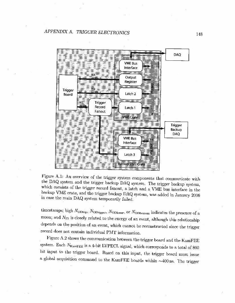
APPENDIX A. TRIGGER ELECTRONICS 148
Figure A.l: An overview of the trigger system components that communicate with the DAQ system and the trigger backup DAQ system. The trigger backup system, which consists of the trigger record fanout, a latch and a VME bus interface in the backup VME crate, and the trigger backup DAQ system, was added in January 2006 in case the main DAQ system temporarily failed.
timestamps; high AoDtop, A ODupper, A^iower, or AoDbottom indicates the presence of a
muon; and AID is closely related to the energy of an event, although this relationship
depends on the position of an event, which cannot be reconstructed since the trigger
record does not contain individual PMT information.
Figure A.2 shows the communication between the trigger board and the KamFEE
system. Each A KamFEE is a 4-bit LVPECL signal, which corresponds to a total of 800
bit input to the trigger board. Based on this input, the trigger board must issue
a global acquisition command to the KamFEE boards within ~400 ns. The trigger

APPENDIX A. TRIGGER ELECTRONICS 149
Trigger Board
LVPECL
Clock
LVPECL
*H
Command
Trigger Command
Fanout
LVPECL
Clock x lO
LVPECL
*H
Command x lO
N- N
LVPECL
KamFEE x200
KamFEE System
Figure A.2: An overview of the communication between the trigger board and the KamFEE system.
Inyyei tiojid
ECL toTTL
LVPECL toLVTTL
1PPS Input
64 bits
448 bits.
Daughterboard 1
( \ . EPC.A ,
v )
5/ bits.
•M8 bits.
Oaughtwho»r«l 2 .. ..
* r r u n "
Clock Driver
W bits.
Daugfetetboafcf 3
r "\
FPGA
\ )
128 bits
16bits_
TTLto ECL
LVTTLto LVPECL
Figure A.3: An overview of the trigger board.
sends the clock and trigger command signals to the trigger command fanout, which
splits them into 10 sets and sends them to the ten KamFEE VME crates.
Figure A.3 shows a schematic of the trigger board. The LVPECL signals from the
KamFEE boards are converted to LVTTL signals before being sent to the FPGA's
(XCV600 by Xilinx). This has two advantages: the converter chips act as a buffer to

APPENDIX A. TRIGGER ELECTRONICS 150
the expensive FPGA chip, and LVTTL signals require only one input line referenced
to ground while LVPECL signals require two input lines. The trigger board receives
800 inputs from the KamFEE boards. However, the largest number of I/O's available
was ~500 at the time the trigger board was designed in 2000, so three FPGA's are
used. Each FPGA is mounted on a separate daughterboard, which can be removed
from the trigger motherboard. Each daughterboard contains all the components
necessary to run the FPGA, and all the other components are contained on the
motherboard. These three daughterboards are identical except for the code stored
on the PROM. This code is transferred to the FPGA on power up. The FPGA's are
reprogrammable, allowing for development of new trigger algorithms. To confirm the
trigger algorithm versions, the DAQ system prompts the trigger board to send the
versions of each FPGA code to latch 2 at the beginning of each run. The FPGA's
perform highly parallel calculations. Two input FPGA's perform initial calculations
and pass the reduced information to a third FPGA. The third FPGA then combines
the information from the first two FPGA's. The third FPGA generates the KamFEE
trigger commands, the MACRO electronics stop commands, and the trigger records.
A buffer, 511 trigger-record deep, incorporated into the third FPGA allows for a
trigger rate of 40 MHz for a brief period. Also, the buffer in latch 1 can contain up
to 12800 trigger records. This is important for detecting a galactic supernova, which
would produce a burst of events. The continuous possible trigger rate depends on the
total data transfer speed, which is limited by the latch 1 to ~40 kHz.

Appendix B
Trigger Types
Triggers are issued for a variety of reasons which can be split into four basic groups:
triggers that issue global acquisition commands to the ID KamFEE boards, triggers
that issue global acquisition commands to the OD KamFEE boards, triggers that
issue stop commands to the MACRO electronics, and other triggers that do not
necessarily issue a trigger command. Two ID KamFEE triggers or two OD KamFEE
triggers are not issued within 200 ns of each other since two triggers in a short period
would record the same waveforms. Most of these triggers can be enabled or disabled.
Most of the trigger types available are described in [27]. Only the trigger types newly
implemented or modified in February 2004 are listed below.
B. l ID KamFEE Triggers
• MACRO to ID Trigger: A global acquisition command is issued to the ID
KamFEE boards when there is a MACRO Singles Trigger. This trigger is
issued 40/xs before the MACRO Singles Trigger. This trigger type is enabled
only during the calibration runs.
151

APPENDIX B. TRIGGER TYPES 152
B.2 MACRO Triggers
• MACRO Calibration Trigger: A short stop command is issued to the MACRO
electronics 20 /xs after every fixed number of calibration device input signals.
This number can be set by the DAQ.
B.3 Other Triggers
• 1PPS Trigger: A trigger record is produced every time the trigger module re
ceives a 1PPS input. The issuing of a global acquisition command to all the
KamFEE boards at the same time can be enabled by the DAQ.
• Supernova Trigger: This is designed to detect the neutrino signal from a super
nova. If the trigger board observes eight events with Any > 772 (before February
2004) or Nm > 1100 (after February 2004) in ~0.84s, this is treated as a su
pernova candidate. After a supernova candidate is observed, the trigger board
sets optimal trigger parameters (supernova mode) to collect as many supernova
events as possible for 1 min before returning to the initial trigger parameters.
Normal trigger parameters would collect most supernova events, but could miss
the important proton scattering events. The rarity of observation of supernova
explosions makes it important to collect as many supernova events as possible.
This trigger is almost always enabled so that supernova events will be collected
even if we are operating with sub optimal trigger parameters. When the DAQ
receives the supernova trigger, it prevents the shift taker from stopping the run
for 1 min.
• Global Calibration Trigger: A global acquisition command is issued to either
the ID or OD KamFEE boards 8 clock-ticks (before February 2004) or 15 clock-
ticks (after February 2004)1 after the trigger board receives an input pulse. The
pulse is generated by a calibration device, such as a LASER, and must arrive
just before the signals from the photons have reached the KamFEE boards.
^ h e 8 clock-tick duration was too short to collect all the light, so it was increased to 15 clock-ticks.

APPENDIX B. TRIGGER TYPES 153
• Run Condition Change Trigger: A trigger record is produced whenever run
conditions are changed by the DAQ or by the supernova trigger. 4& *ite

APPENDIX B. TRIGGER TYPES 154
Appendix C
Absolute Time Acquisition System
Knowing the absolute time for each event is important to compare results on a com
mon source, such as a supernova, with other experiments. In KamLAND, the absolute
time is obtained from a Global Positioning System (GPS) receiver (Model 600-000
manufactured by TrueTime). As shown in Figure C.l, the GPS receiver and its an
tenna are located outside the mine to receive signals from the GPS satellites, to which
the GPS receiver's internal clock locks. When receiving signals from at least 4 GPS
satellites, the GPS receiver calculates the absolute time to an accuracy of 100 ns of
Universal Time Co-ordinates (UTC). Even when the GPS receiver does not receive
signals from any satellite, it continues to calculate the time using its internal clock.
The status of the GPS receiver, such as the number of GPS satellites the GPS receiver
is tracking, is checked every 60s by a computer using the serial port from the GPS
receiver. This information is only used to monitor the GPS receiver and is not sent
to the main DAQ system.
The absolute time, encoded in a serial digital format (IRIG-B), and One Pulse Per
Second (1PPS) signals, generated as TTL signals by the GPS receiver, are converted
into optical signals and sent to the electronics hut inside the mine through optical
fibers. Inside the electronics hut, these signals are converted back to TTL signals.
The 1PPS signal is sent to the trigger board, and the encoded time is sent to a
GPS VME interface (Model 560-5608 VME-SG2 manufactured by TrueTime), which
synchronizes its internal clock to the received time code. The GPS VME interface
155
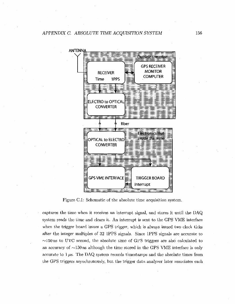
APPENDIX C. ABSOLUTE TIME ACQUISITION SYSTEM 156
ANTENNA
r~ RECEIVER
Time 1PPS
Outside the mine
GPS RECEIVER MONITOR
COMPUTER
ELECTRO to OPTICAL CONVERTER
fiber
OPTICAL to ELECTRO CONVERTER
Electronics Hut inside the mine
^ r GPS VME INTERFACE TRIGGER BOARD
Interrupt
Figure C.l: Schematic of the absolute time acquisition system.
captures the time when it receives an interrupt signal, and stores it until the DAQ
system reads the time and clears it. An interrupt is sent to the GPS VME interface
when the trigger board issues a GPS trigger, which is always issued two clock ticks
after the integer multiples of 32 1PPS signals. Since 1PPS signals are accurate to
~150ns to UTC second, the absolute time of GPS triggers are also calculated to
an accuracy of ~150ns although the time stored in the GPS VME interface is only
accurate to 1 /j,s. The DAQ system records timestamps and the absolute times from
the GPS triggers asynchronously, but the trigger data analyzer later associates each
APPENDIX C. ABSOLUTE TIME ACQUISITION SYSTEM 157
GPS trigger timestamp with its corresponding absolute time. The absolute time of
any event can be calculated with the difference in the timestamps between an event
and its nearest 1PPS trigger. The frequency of the trigger board clock drifts slightly
depending on various factors such as temperature. However it drifts only about 10 ns
per second.
The signal delay time between the GPS receiver and the electronics hut has been
measured from the time a pulse takes to make a round trip. Outside the mine, a TTL
signal was converted into an optical signal, and sent to the electronics hut through an
optical fiber. The signal received in the electronics hut is converted to a TTL signal
and then to an optical signal, and sent back to outside of the mine through an optical
fiber. The signal is then converted back to a TTL signal outside the mine. Half of
the time difference between the initial pulse and the returned pulse was 21.4/zs, then
changed to 12.0//s in November 2005, when the GPS receiver was relocated because
of a rerouting of the optical fibers.

APPENDIX C. ABSOLUTE TIME ACQUISITION SYSTEM 158
.».»
Appendix D
Event Position Reconstruction
Algorithm
The position of an event is first roughly estimated using the distribution of the PEs
produced in the PMTs, then fine tuned using the times photons take to travel from the
event position to the PMTs in a straight path. Some fraction of photons produced in
an event are absorbed at some point along their path and then reemitted in a random
direction. These reemitted photons do not yield the event position. Therefore the
algorithm mostly uses photons that traveled directly from the event position to PMTs
by selecting pulses in the initial peak of arrival time distribution after correcting for
the expected flight time. The algorithm follows the steps described below:
1. Only the pulses from Hamamatsu RS7250 PMTs are selected. Pulses with
less than 0.2 PEs are discarded to avoid contamination from false pulses from
electrical noise. If multiple waveforms from one PMT are recorded, pulses
extracted from the waveform with the lowest gain are chosen.
2. If there are less than 4 pulses remaining in the event, the algorithm does not
try to fit any further, and exits with a status "Unknown."
3. The initial rough position estimate is made using the distribution of the PEs
159
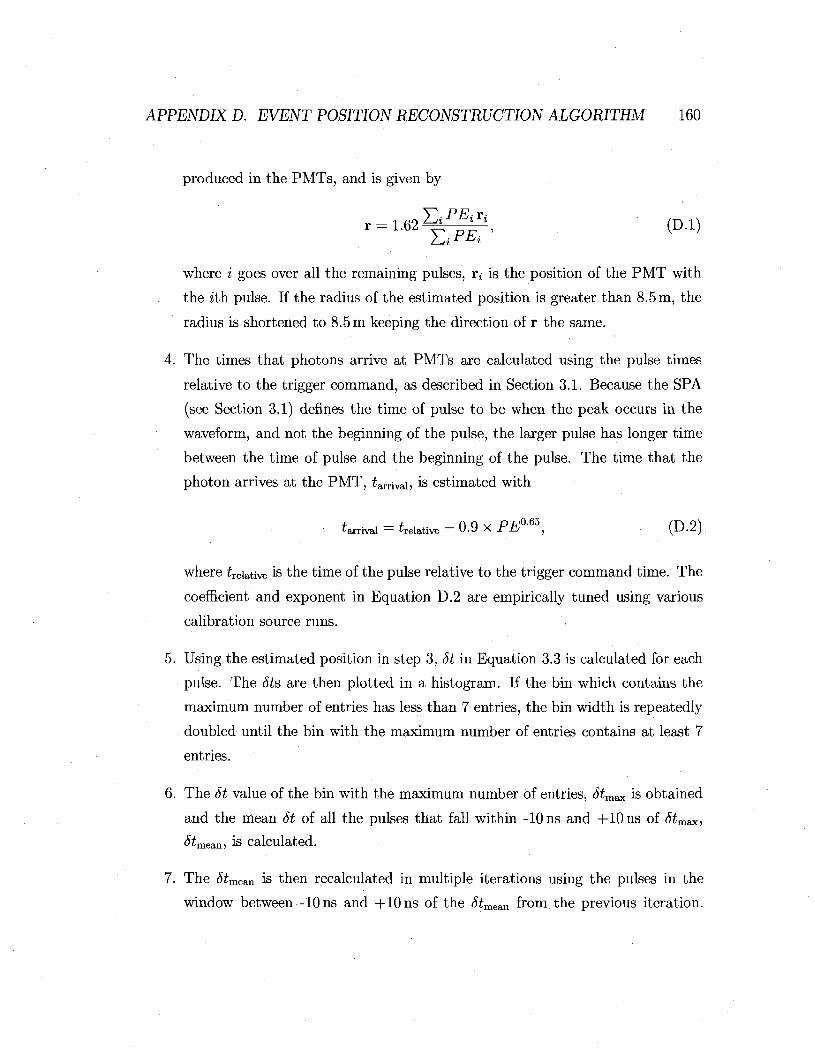
APPENDIX D. EVENT POSITION RECONSTRUCTION ALGORITHM 160
produced in the PMTs, and is given by
r ^ l . 6 2 ^ ^ , (D.l)
where i goes over all the remaining pulses, rj is the position of the PMT with
the ith pulse. If the radius of the estimated position is greater than 8.5 m, the
radius is shortened to 8.5 m keeping the direction of r the same.
4. The times that photons arrive at PMTs are calculated using the pulse times
relative to the trigger command, as described in Section 3.1. Because the SPA
(see Section 3.1) defines the time of pulse to be when the peak occurs in the
waveform, and not the beginning of the pulse, the larger pulse has longer time
between the time of pulse and the beginning of the pulse. The time that the
photon arrives at the PMT, iarrivab is estimated with
^arrival = ^relative ~ 0.9 X PE ' , (D .2 )
where Relative is the time of the pulse relative to the trigger command time. The
coefficient and exponent in Equation D.2 are empirically tuned using various
calibration source runs.
5. Using the estimated position in step 3, St in Equation 3.3 is calculated for each
pulse. The 5ts are then plotted in a histogram. If the bin which contains the
maximum number of entries has less than 7 entries, the bin width is repeatedly
doubled until the bin with the maximum number of entries contains at least 7
entries.
6. The 8t value of the bin with the maximum number of entries, Stmax is obtained
and the mean 5t of all the pulses that fall within -10 ns and +10 ns of 5tmax,
<5imean, is calculated.
7. The 5tmea,n is then recalculated in multiple iterations using the pulses in the
window between -10 ns and +10 ns of the <5imean from the previous iteration.

APPENDIX D. EVENT POSITION RECONSTRUCTION ALGORITHM 161
This process is repeated until the difference between the $£means from the current
and the previous iterations is less than 0.1 ns, or 100 iterations are performed.
8. Using only the pulses in the peak time window, -10 ns and +5ns around the
Stmeim calculated in step 7, the current estimated event position is pushed ac
cording to the vector given by
Ar = £(fc,-<&»f^-, (D.3) ^travel, i
where i goes over all the pulses in the peak time window, r is the current esti
mated position, ttraveU *s *n e t i m e of travel from the current estimated position
to the PMT with the ith pulse, Sti is the St of the ith pulse, and (St) is the
mean St in the peak time window. The event position, (St), and peak time
window are recalculated in each of multiple iterations. After the first iteration,
the peak time window is defined to be -10ns and +5ns around (St). The itera
tions continue until the distance between the current estimated position and the
estimated position in the previous iteration is less than 1 mm, or 100 iterations
are performed.
9. After step 8, the reconstruction status is assigned based on various factors.
There are three variables to assess the quality of the fit: /RMS, /peak pulse ratio >
and fpeakRMS- IRMS is the RMS of the St distribution, /peakpuiSeratio is the
fraction of the pulses in the peak time window, and fpeakRMS is the RMS
of the St distribution in the peak time window. Table D.l summarizes the
reconstruction status. An event can have multiple statuses if the reconstruction
fails due to multiple factors, as described in Table D.l.
10. If the status assigned in step 9 is "Bad," and none of the other factors failed,
then step 8 is repeated using the current estimated position and (St). The status
is reassigned depending on the result of this step.
11. If the radius of the reconstructed position is greater than 10 m, the position is

APPENDIX D. EVENT POSITION RECONSTRUCTION ALGORITHM 162
Table D.l: Position reconstruction status
Status type Description Valid Successful reconstruction. Unknown Number of pulses < 4. Not valid Reconstructed radius > 10 m. Bad The fit did not converge. Bad fRMS fRMS < 35 or fRMS > 90. B a d /peak pulse ratio /peak pulse ratio
< 0.22 or /P e a k
pulse ratio > 0.55.
B a d f Peak RMS fPeak RMS < 1-7 Or fPeak RMS > 4
adjusted. The new position, rnew, is given by
rnew = r (D.4) |r[m]|
Using rnew and the (5t), step 8 is repeated, and the status is reassigned depend
ing on the result of this step.
The ranges for which fRMs, /peak pulse ratio, and fpeakRMS are valid are determined
using the distributions of these variables for the events which are believed to be
point-like events compared with muons or noise events caused by muons. These
variables are designed to eliminate muons and noise following muons, such as after-
pulses. Figure D.l shows the distributions of fRMs, /peak pulse ratio, and fPeakRMS for
events with A viaxiD above 200 during normal run 394. The valid ranges, indicated
by the vertical dotted lines, reject large fractions of muons or post muon noises while
remaining the other events.

APPENDIX D. EVENT POSITION RECONSTRUCTION ALGORITHM 163
a j B ^ a r i B a l B B l a
0.8 0.9
Figure D.l: fRMS (top plot), /Peak pulse ratio (middle plot), and fPeakRMS (bottom plot) distributions for events from normal run 394. The thick solid lines are for all the events with A^axiD above 200. The thin solid lines are for events tagged as Muons or Post Muon Noise (see Section 3.6). The dotted lines indicate the valid ranges.

APPENDIX D. EVENT POSITION RECONSTRUCTION ALGORITHM 164
Appendix E
Energy Calibration Points
The measurements used to fit the model of Ev-ls/Erea,i (see Section 3.4) are described
below. The calibration points are defined to be EV[S at the center of detector, and its
error includes temporal and spatial uncertainties. Many of the calibration points are
estimated using radioactive sources deployed in the LS (see Section 2.4).
E. l 203HgjE;v i s
Evis calibration point of 203Hg is estimated by fitting a Gaussian function to the
.Evis distribution of the 7s from the 203Hg source deployed at the center. The time
variation of 1,4% is estimated to be the same as the Evis time variation of 214Po
a-decays, described in Section E.7. In addition, a conservative error of 1.8% due to
the position uncertainty is estimated by comparing the Evi8 means obtained from the 203Hg source deployed at the center and 1 3 m1. The estimated Evis calibration point
of 203Hg is 0.2400 ± 0.0055 MeV.
E.2 68Ge .Evis
EviS calibration point of 68Ge is estimated by fitting a Gaussian function to the Ev-ia
distributions of the 7s from the 68Ge source deployed at the center in various runs. 1 Unlike other source calibrations, there is no calibrations at ±1 m for 203Hg source.
165
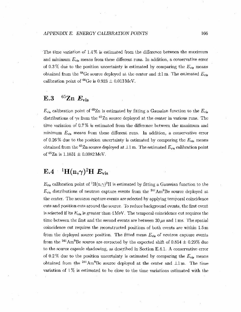
APPENDIX E. ENERGY CALIBRATION POINTS 166
The time variation of 1.4% is estimated from the difference between the maximum
and minimum Evi8 means from these different runs. In addition, a conservative error
of 0.3 % due to the position uncertainty is estimated by comparing the E^ means
obtained from the 68Ge source deployed at the center and ±1 m. The estimated EviS
calibration point of 68Ge is 0.923 ± 0.013 MeV.
E.3 65Zn Evis
Evis calibration point of 65Zn is estimated by fitting a Gaussian function to the Ev\s
distributions of 7s from the 65Zn source deployed at the center in various runs. The
time variation of 0.7% is estimated from the difference between the maximum and
minimum Evi8 means from these different runs. In addition, a conservative error
of 0.26 % due to the position uncertainty is estimated by comparing the _Evis means
obtained from the 65Zn source deployed at ±1 m. The estimated Evis calibration point
of 65Zn is 1.1031 ± 0.0082 MeV.
E.4 'EKn^H Evis
Evis calibration point of 1H(n,7)2H is estimated by fitting a Gaussian function to the
Evis distributions of neutron capture events from the 241Am9Be source deployed at
the center. The neutron capture events are selected by applying temporal coincidence
cuts and position cuts around the source. To reduce background events, the first event
is selected if its Evis is greater than 4 MeV. The temporal coincidence cut requires the
time between the first and the second events are between 30 /is and 1 ms. The spatial
coincidence cut requires the reconstructed positions of both events are within 1.5 m
from the deployed source position. The fitted mean EV-1S of neutron capture events
from the 241Am9Be source are corrected by the expected shift of 0.854 ± 0.29% due
to the source capsule shadowing, as described in Section E.4.1. A conservative error
of 0.2% due to the position uncertainty is estimated by comparing the Ev[s means
obtained from the 241Am9Be source deployed at the center and ± l m . The time
variation of 1 % is estimated to be close to the time variations estimated with the
APPENDIX E. ENERGY CALIBRATION POINTS 167
J i i — J I u _ i • I • i J I • „ • • • • ' ' I • • • I ' i • L_J
"-6000 -4000 -2000 0 2000 4000 6000 Simulated source z-position [mm]
Figure E.l: Reconstructed mean Evis differences for simulated 241Am9Be neutrons with and without 241Am9Be source capsule at various source positions along the z-axis. The thick horizontal line is a flat line fit to these mean Evia fractional differences from -5500 m to 5500 m. The fit yields a shift of 0.854 ± 0.050%. The x2/n.d./. of this fit is 13.2/12.
68Ge (see Section E.2) and 65Zn (see Section E.3) sources. The estimated Evia of
^ ( n ^ H calibration point is 2.333 ± 0.025 MeV.
E.4.1 241Am9Be Source Shadowing Estimation
The reconstructed Evis of 241Am9Be neutron capture events needs to be corrected
to account for the shadowing of the deployment equipments such as the source cap
sule. The amount of the shadowing is estimated by simulating the 241Am9Be source
with and without the deployment equipment at various positions along the z-axis
using KLG4sim. The simulated data is then reconstructed using the default event
reconstruction algorithms. The percentage difference of reconstructed E^s of these
simulated events at various z-positions are fairly constant, as shown in Figure E.l.
The shadowing effect is estimated to be 0.854 ± 0.29% by fitting a constant across
the z-positions and taking the maximum variation.
£ Z|
o a
w
g +-» a o o <D
Pi
1.5
0.5

APPENDIX E. ENERGY CALIBRATION POINTS 168
L E
vent
400
200
0
-
i , , 4.8
, 1 ,
5 , , i ,
5.2 5.4 5.6 , I , 5.8
. " Z . 1
, , 1 ,
E™ [MeV]
Figure E.2: The background subtracted Evia of spallation neutron capture on 12C. The Gaussian function fit (solid line) yields the mean of 5.476 ± 0.014 MeV. The X2/n.d.f. of this fit is 5.8/4.
E.5 60 Co E^ VIS
Since the reconstructed Evis is calibrated to be the same as the Ereai = 2.50572 MeV
of 60Co, only the position uncertainty is considered. A conservative error of 0.37% is
estimated by comparing the E^s means of 7s from the 60Co source deployed at the
center and ±1 m. The estimated EYis calibration point of 60Co is 2.5057 ± 0.0093 MeV.
13, E.6 12C(n,7)13C E VIS
Eyis calibration point of 12C(n,7)13C is estimated using the spallation neutrons, cap
tured on 12C. The events are selected by temporal coincidence with muons. The
neutron capture candidate events are selected between 0.2 ms and 1.2 ms after muons,
while background events to be subtracted from the neutron capture candidate events
are selected between 1.2 ms and 5.2 ms after muons. The neutron capture events are
selected within the reconstructed radius of 4.7 m. Figure E.2 shows the background

APPENDIX E. ENERGY CALIBRATION POINTS 169
subtracted Eyis distribution and a Gaussian function fit to this distribution. There
are two types corrections that need to be applied to the mean from this Gaussian
function fit. The first is the Ev-18 reconstruction bias after muons. The fitted mean
Evis is shifted down by 0.72 ± 0.17%, estimated in Section 3.3.1. The other correc
tion is the Evis reconstruction bias due to the position of the events. Since all the
events are selected within 4.7 m, the Ey[s at the center needs to be estimated. This
is done by comparing the reconstructed EViS for spallation neutrons, captured on ^
within 4.7m radius after correcting for after muon effect (see Section 3.3.1) to the
Evis of neutron capture events from the 241Am9Be source deployed at the center after
correcting for the 241Am9Be capsule shadowing effect (see Section E.4.1). The EviS
shift necessary due to the position variation is 0.54 ± 0.54%. The time variation
of 1 % is estimated to be close to the time variation estimated with the 68Ge (see
Section E.2) and 65Zn (see Section E.3) sources. The estimated EViS calibration point
of 12C(n,7)13C is 5.407 ± 0.063 MeV.
E.7 214Po a-decay EVls
214Po a-decays can be selected using the coincidence with 214Bi /3-decays. 214Bi j3-
decays with an endpoint of 3.272 MeV. Then the daughter nucleus, 214Po, a-decays
with Q = 7.833 MeV and half-life of 164.3 [is. The following cuts are applied to select
the 214Po cu-decay events; the 214Bi /?-decay EViS is between 1.5 MeV and 5 MeV,
the distance between the 214Bi /?-decay and 214Po a-decay events is less than lm,
and the time between these events is between 0.5 /xs and 1ms. Both events are also
required to be within 1 m from the center of the ID. The top plot in Figure E.3
shows distribution of the time difference between the 214Bi /?-decay and 214Po a-
decay candidates. The fitted half-life of 167.2 ± 3.4 [is is consistent with the nominal
value of 164.3//s. The bottom plot in Figure E.3 shows the Evis distribution of 214Po
a-decay events. The mean Evis of 0.62006 ± 0.00098 MeV is obtained by fitting a
Gaussian function. The Evi8 error of 0.67% due to the position uncertainty is taken
by comparing the events within 1 m radius to within the spherical shell of between
1 m and 2 m radius. Figure E.4 shows the ~1.4 % time variation of mean E^ of 214Po

APPENDIX E. ENERGY CALIBRATION POINTS 170
100 200 300 400 500 600 700 800 900 1000 At [|xs]
>
i n I N
P300 o
> c3
200
100
-—
"
_
-
+
J \
I M M I U I . I M I I l > K . i i l n i h i l 0.4 0.45 0.5 0.55 0.6 0.65 0.7 0.75 0.8 0.85 0.9
E^JMeV]
Figure E.3: 214Po a-decay candidates within 1 m from the center of the ID. The top plot shows the t ime difference between the 2 1 4Bi /3-decay and 2 1 4 Po a-decay events. The exponential fit yields the half-life of 167.2 ± 3.4 /is with a x2/n.d.f. of 4.7/8. The bottom plot shows the Evis distribution. The Gaussian function fit yields the mean of 0.62006 ± 0.00098 MeV, and sigma of 0.05412 ± 0.00076 MeV with a %2/n.d./. of 24.0/29

APPENDIX E. ENERGY CALIBRATION POINTS 171
-SI S
1000 2000 3000 4000 5000 6000 Run number
Figure E.4: Evis time variation of 214Po a decay candidates within 3 m from the center of the ID. Approximately 1.4% variation is seen.
a-decay events within a 3 m radius. The estimated Evis calibration point of 214Po
a-decay is 0.6201 ± 0.0097 MeV.
E.8 ^ P o a-decay E VIS
212Po a-decays can be selected using the coincidence with 212Bi /^-decays. 212Bi /?-
decays with an endpoint of 2.25 MeV. Then the daughter nucleus, 212Po, a-decays
with Q = 8.954 MeV and half-life of 0.299 /xs. The following cuts are applied to select 212Po a-decay events; the 212Bi /3-decay Evis is between 1 MeV and 2.6 MeV, the
distance between the 212Bi /3-decay and 212Po a-decay events is less than 1 m, and the
time between these events is between 0.5 /xs and 1 /xs. Both events are also required to
be within 3 m from the center of the ID. The top plot in Figure E.5 shows distribution
of the time difference between the 212Bi /5-decay and 212Po a-decay candidates. The
fitted half-life of 0.45 ± 0.15/xs is consistent with the nominal value of 0.299/xs. The
bottom plot in Figure E.5 shows the Evis distribution of 212Po a-decay events. The
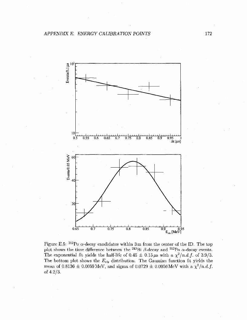
APPENDIX E. ENERGY CALIBRATION POINTS 172
102
>
10 0.5 0.55 0.6 0.65 0.7 0.75 0.8 0.85 0.9 0.95 1
At [us]
60
o p
> 4 0 -
20-
0.65 0.7 0.75 0.8 0.85 0.9 0.95 , [MeV]
Figure E.5: 212Po a-decay candidates within 3 m from the center of the ID. The top plot shows the time difference between the 212Bi /?-decay and 212Po a-decay events. The exponential fit yields the half-life of 0.45 ± 0.15 ^s with a x2/n.d.f. of 3.9/3. The bottom plot shows the EY{S distribution. The Gaussian function fit yields the mean of 0.8136 ± 0.0059 MeV, and sigma of 0.0729 ± 0.0056 MeV with a X2/n.d.f. of 4.2/3.
APPENDIX E. ENERGY CALIBRATION POINTS 173
error due to the position variation is estimated from the percentage difference in
the Ev[s means obtained with the captures of neutrons from the 241Am9Be source
deployed at the center and 3 m. The time variation of 1.4% is chosen to be the same
as that of 214Po cn-decays. The estimated Evis calibration point of 212Po a-decays is
0.806 ± 0.013 MeV.

APPENDIX E. ENERGY CALIBRATION POINTS 174
Appendix F
Spallation Product Selection Cuts
The cuts to select spallation products, 12B and neutrons, used in Chapter 4 are
described in the following sections. See Section 3.6 for the definitions of the various
events tags used in these cuts.
F.l 12B
The 12B /?-decay candidates are selected using the following cuts:
• The 12B /3-decay candidate event has valid position and E^s reconstruction
statuses.
• The 12B /?-decay candidate event has Evis above 4MeV. Although the Evls
spectrum of 12B /3 spans below 4 MeV, background events overwhelm Evia below
4MeV.
• The 12B /?-decay candidate event is not tagged as a Muon.
• The 12B /?-decay candidate event follows within 2 to 52 ms of the last muon.
• Events for background subtraction follow within 52 to 202 his of the last muon.
• The associated muon event is tagged as both OD and ID Muon, which does
not follow and is not followed by another event tagged as an ID Muon within
175

APPENDIX F. SPALLATION PRODUCT SELECTION CUTS 176
202 ms. This timing restriction is to ensure each of the selected 12B /?-decay
candidates and background events are associated with only one muon.
F.2 Neutrons
Different sets of cuts are used to select spallation neutron candidate events in the
capture spaii, the reconstructed Evis distribution, and the reconstructed radial distribu
tion studies. Most of the differences are to optimize the selection of neutron capture
events for a specific study1. The common cuts to all of these studies are that the
associated muon does not follow and is not followed by another event tagged as a ID
Muon within 0.1s, and the neutron capture candidate event has valid position and
EV1S reconstruction statuses. The differences are described in the following sections.
F.2.1 Neutrons for TcaptUre, spall Est imation
In order to estimate rcapture, spall, spallation neutrons are selected using the following
additional cuts:
• The associated muon is tagged as a LS Muon and has a A MaxiD greater than
1250 to ensure that it is indeed a LS muon, but not tagged as a Shower Muon
since large charge deposits from Shower Muons affect the detector performance
for a long time afterwards.
• The neutron capture candidate event has a NMBXIB between 400 and 490, and
reconstructed EV-1S between 1.4'MeV and 3.4 MeV to reduce the contamination
from 12B (3-decays2.
• The neutron capture candidate event is reconstructed within the fiducial volume
of 5.5 m radius to avoid bias in the estimated rcapture, spall due to the rcapture, spaii
difference in the LS and buffer oil. 1Some of the cuts, EV-1S window for example, happen to differ slightly in each study since the stud
ies are conducted separately although these slight differences would not make noticeable difference in the results.
2See Section 4.1 for more details on 12B /3-decays.

APPENDIX F. SPALLATION PRODUCT SELECTION CUTS 111
F.2.2 Neutrons for EV-1S Estimation
In orcjer.to estimate the mean capture Evis, spallation neutrons are selected using the
following additional cuts:
• The associated muon is tagged as a LS Muon and has a A MaxiD greater than
1250 to ensure that it is indeed a LS muon, but not tagged as a Shower Muon
since large charge deposits from Shower Muons affect the detector performance
for a long time afterwards.
• The neutron capture candidate events and background events are taken from
0.8 ms to 1.2 ms, and 1.2 ms to 5.2 ms after the previous muons, respectively.
The events that closely follow muons are avoided to reduce possible effects from
the Evis bias due to the electronics baseline shift after muons.
F.2.3 Neutrons for Position Distribution Estimation
To obtain reconstructed radial distribution, spallation neutrons are selected using the
following additional cuts:
• The associated muon is tagged as both OD and ID Muon.
• The neutron capture candidate and background events follow within 0.8 to
1.2 ms and 1.2 to 5.2 ms of the last muon, respectively. The events that closely
follow muons are avoided to reduce possible effects from the EYia bias due to
the electronics baseline shift after muons.
• The neutron capture candidate and background events have Evia between 1.5
and 3.5 MeV.
• The neutron capture candidate and background events are not tagged as an OD
Muon.
• The A iaxiD of the neutron capture candidate event is greater than 200 (period I)
or 180 (period II).

APPENDIX F. SPALLATION PRODUCT SELECTION CUTS 178
Appendix G
^MaxID Threshold Efficiency
Calculation
The details of the estimation of £jvMaxiD a r e discussed below.
- MaxiD depends on both the Evis and position of an event; the larger the radius, the
larger the Evis for the same A MaxiD) a s shown in Figure G.l. Therefore £wMaxID(-£'vi8)
(see Equation 5.3) is estimated for period I and II in each of three concentric regions
in the detector: r < 4.7m, 4.7m < r < 5.5m, and 5.5m < r < 6.3m as shown in
Figure 5.4. The £jvMaxiD(-Evis) is obtained using run 3888, which is a special run with
a low trigger N^ threshold of 35; since the mean reconstructed Evis of events whose
- MaxiD is equal to 35 is ~0.1MeV, the £ArMaxID(-Evis) distribution distortion around
the analysis Evis thresholds of 0.9 MeV and 0.8 MeV in periods I and II, respectively,
caused by the detector Nm threshold of 35 is negligible. An error function is fitted
to only some portion of each £ArMaxID(£'vis) to approximate the shape. The means,
jvMaxiD) a n d sigmas, crjvMaxiD> °f the fitted error functions are shown in Table G.l.
The relation between Evis and iVMaxiD, shown in Figure G.l, can change depending
on the scintillation level at a given time due to various factors such as the oxygen
content and temperature in the LS. This change can affect the values of /JjvMaxiD an<^
o/VMaxiD- Their time variations are estimated using the time variations of means and
RMS of the EY[S of events whose A^axiD is equal to the analysis A MaxiD threshold.
Table G.2 summarizes such Evis means and RMS from run 3888. Figure G.2 shows
179
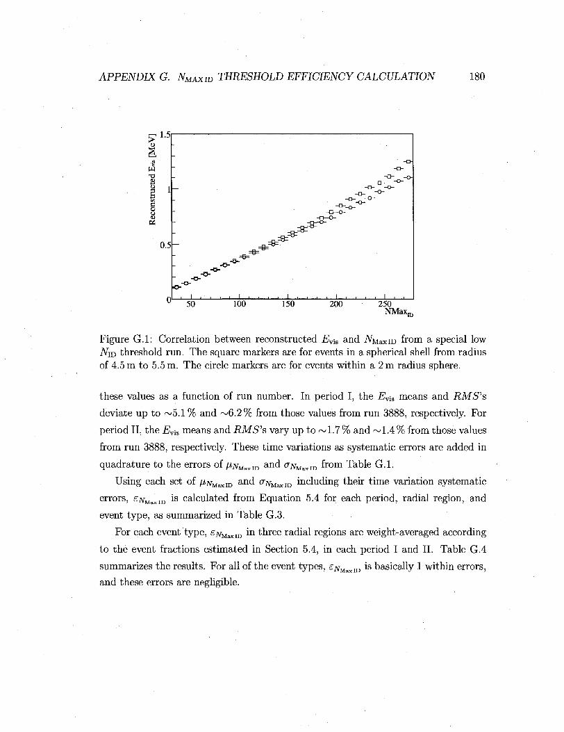
APPENDIX G. NMAXID THRESHOLD EFFICIENCY CALCULATION 180
r1-5
a o 8 ex
0.5
_Q_ - O -
u * " . ^
-J I I U • • ' •
50 100 150 200 250 NMax„
Figure G.l: Correlation between reconstructed Ev\s and AW* ID from a special low iViD threshold run. The square markers are for events in a spherical shell from radius of 4.5m to 5.5m. The circle markers are for events within a 2m radius sphere.
these values as a function of run number. In period I, the Evis means and RMS's
deviate up to ~5 .1% and ~6.2% from those values from run 3888, respectively. For
period II, the E^ means and i?MS"s vary up to ~ 1.7 % and ~1.4 % from those values
from run 3888, respectively. These time variations as systematic errors are added in
quadrature to the errors of A*jvMaXiD a n d ^NM^I-D frorn Table G.l.
Using each set of /UjvMaxID and cjvMaxID including their time variation systematic
errors, £jvMaxiD *s calculated from Equation 5.4 for each period, radial region, and
event type, as summarized in Table G.3.
For each event type, £jvMaxro m three radial regions are weight-averaged according
to the event fractions estimated in Section 5.4, in each period I and II. Table G.4
summarizes the results. For all of the event types, £jvMaxiD is basically 1 within errors,
and these errors are negligible.

APPENDIX G. NMAXID THRESHOLD EFFICIENCY CALCULATION 181
TableG.l: The fitted MiVMaxiD an<^ aiVMaxiD obtained from run 3888 with the low NJQ
threshold. A W ID threshold r ran'ge [m] fiNt/ [MeV] VN*, [MeV]
200
180
r < 4.7 4.7 < r < 5.5 5.5 < r < 6.3
r < 4.7 4.7 < r < 5.5 5.5 < r < 6.3
0.7803 ± 0.0016 0.8140 ± 0.0037 0.9119 ±0.0036 0.6854 ±0.0013 0.7168 ±0.0018 0.7876 ± 0.0029
0.0341 ± 0.0019 0.0454 ± 0.0035 0.0880 ± 0.0034 0.0387 ±0.0015 0.0458 ± 0.0022 0.0877 ± 0.0031
Table G.2: The mean and RMS of EV1S for events with AWciD = 200 and AWciD 180 from the special low iNfo threshold run 3888.
A W ID £vis mean [MeV] Evis RMS [MeV]
200 180
0.7804 0.6837
0.0453 0.0355
Table G.3: £jvMaxiD f°r va ri°us event types in three radial regions. The errors are given in parenthesis.
Event type r range [mm] £jvMaxID period I £ % M l D period II
^reactor
238 UP, geo
232> T h ^
13 C(a, n) (p scattering)
r < 4.7 4.7 < r < 5.5 5.5 < r < 6.3
r < 4.7 4.7 < r < 5.5 5.5 < r < 6.3
r < 4.7 4.7 < r < 5.5 5.5 < r < 6.3
r < 4.7 4.7 < r < 5.5 5.5 < r < 6.3
1.0000000(26) 0.999993(75) 0.9989(11)
1.000000(38) 0.9999(10) 0.986(15)
0.999999(99) 0.9997(26)
0.964(0.038) 1.00000(29) 0.9993(62) 0.960(40)
0.999999983(56) 0.9999992(14) 0.999845(71) 0.9999998(77) 0.999989(18) 0.9980(92)
0.9999994(20) 0.999972(47) 0.9948(24)
0.999978(66) 0.9992(10) 0.9912(88)

APPENDIX G. NMAxm THRESHOLD EFFICIENCY CALCULATION 182
^ 0 . 8 5 u
s S 0.8
J •a
0.75 d o o 04
0.7
^ V * *4
P^^^v»^^ ;^«H -J I I I I I L_ L63) 1000 2000 3000 4000 5000 6000
Run number
0.055|
0.05
10.045
8 0.041
0.035
0.0$
^"P^WKij^tei^jg.,
m X J I I L.
1000 2000 3000 4000 5000 6000 Run number
Figure G.2: Means (top plot) and RMS (bottom plot) of the reconstructed Evia
for all the events with ATMaxID equal to the analysis iVMaxiD threshold. The vertical dotted line separates the two periods with ATMaxID threshold of 200 (period I) and 180 (period II). Two horizontal dashed lines before and after run 3611 indicate the mean (top plot) and RMS (bottom plot) of Evis at A^axiD equal to the analysis iVMaxID
threshold, taken from run 3888, the special low threshold run.

APPENDIX G. NMAX m THRESHOLD EFFICIENCY CALCULATION 183
Table G.4: SNM ID for various event types. The errors are given in parenthesis.
Event type £JVMaxin P e r i o d I £ivMaxin P e r i o d II ^reactor 238U ugeo 232Th Pgeo 13C(a,n)160 (p scattering)
0.999954(54) 0.99941(70) 0.9984(18) 0.9976(27)
0.9999934(30) 0.999914(38) 0.99978(10) 0.99837(51)

APPENDIX G. NMAXID THRESHOLD EFFICIENCY CALCULATION 184

Appendix H
Reconstruction Efficiency
Calculation
The details on the calculation of ereCon a r e described below.
Brecon is estimated as the fraction of events with "reasonable reconstruction," de
fined in Table H.l, using the 60Co68Ge and 241Am9Be sources with known energies and
deployed positions, and the events acquired during normal runs. The reconstruction
efficiency for the source events, erecon,source, is calculated by properly subtracting the
background events obtained from a normal run without the source, and is given by
1 'recon, source ±'recon, BG /TT -. \ Brecon, source — "TJ 77 j V *!••'-J
^A^Max ID, Source ~ "^ iVMaxID.BG
where Nrecon> source and ./Vrecon.BG denote the number of events that pass all the cuts
in Table H.l and have valid statuses returned by the reconstruction algorithms in
the source and normal runs, respectively. JVjvMaxID)source and -/VjvMaxID)BG denote the
number of events that pass only the A^axiD cut in the source and normal runs,
respectively.
Figure 5.5 shows erecon,source at various positions along the vertical central axis
of the detector for 60Co68Ge and 241Am9Be sources, each of which indicates that
Brecon, source is reasonably constant across various positions. erecon,source for 60Co68Ge
185

APPENDIX H. RECONSTRUCTION EFFICIENCY CALCULATION 186
Table H.l: Cuts for evaluating £recon,source of "reasonable reconstruction."
Source AM^ID Evis [MeV] Position [m] 60Co68Ge 180 < iVMaxiD < 600 0.5 < Evis < 3.5 |rsource - r recon | < 1.5 241Am9Be 600 < NMaxlD < HOP 2 < £vis < 12 lrsource - rreConl < 2.5
and 241Am9Be are estimated by fitting a constant to the Brecon, source at various posi
tions, resulting in 0.99986 ±0.00020 and 0.99747 ±0.00012, respectively. The average
of these two fitted erecon,sources is 0.998665 ± 0.00012.
The error of £recon is estimated by comparing erecon, source with the reconstruction
efficiency for events during normal runs, Brecon, normal, whose true positions and Eyia
are not known. The iVMaxiD of radioactivity during normal runs spans up to A MaxiD
of ~450, so Brecon,normal is estimated using the events whose NMaxm is between 200
(period I) or 180 (period II) and 450. Since the exact position or Evis of the radioactive
background events are not known, £recon, normal, is calculated from
Brecon, normal — ~T7 , K^---^)
where iVvaiid denotes the number of events that pass the iVMaxiD cut and the Cosmo-
genic Spallation Cuts, defined in Section 5.3.2, and have valid statuses returned by
the reconstruction algorithms, and -WjvMaxID denotes the number of events that pass
the NuaxiD cut and the Cosmogenic Spallation Cuts.
Figure H.l shows £reCon, normal a s a function of iVMaxID for all the good runs in
periods I and II. The events with low ATMaxID have slightly lower £reCon, normal due to
lack of photons produced in the LS for low Evis events. Figure 5.6 shows the time
variation of £reCon,normal- The maximum deviation of erecon,normal at various iVMaxiD
and time from £reCon,source is 0.0022, which is taken as the error of £recon, resulting in
an estimated £recon of 0.9987 ± 0.0022.
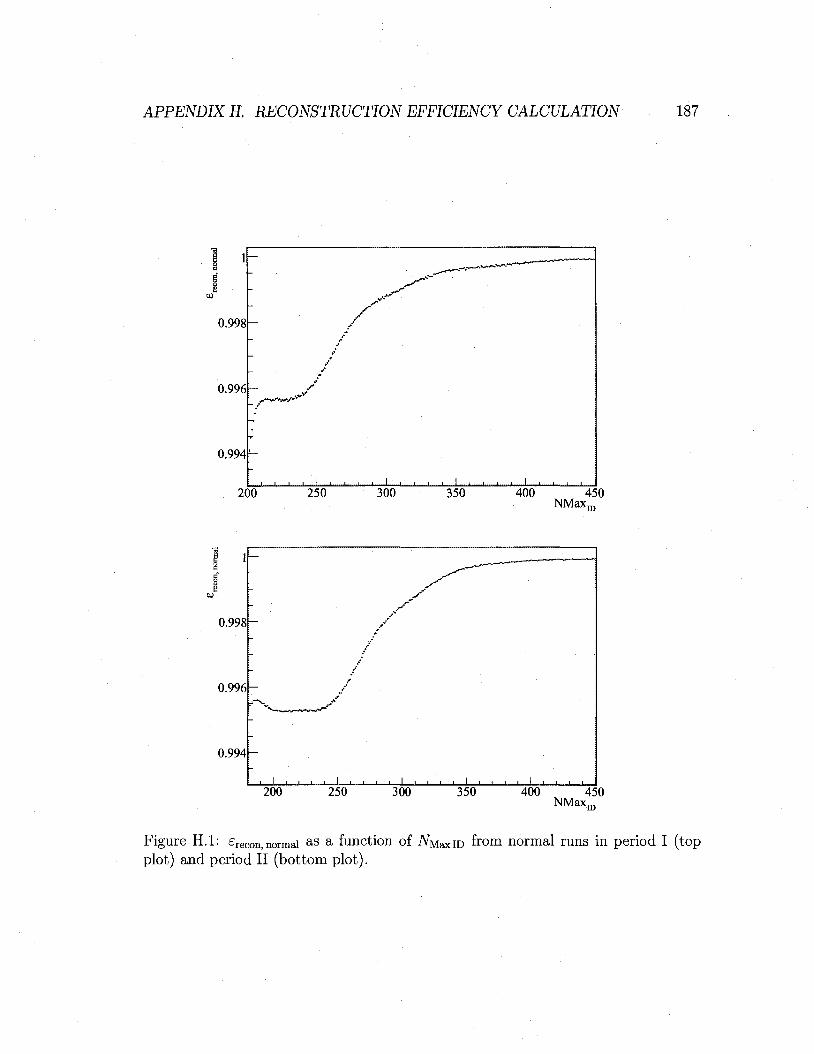
APPENDIX H. RECONSTRUCTION EFFICIENCY CALCULATION 187
l h
/ 0.998h
0.996h
0.994F
200 250 ' • - ' -i I - - ' i I . I I • ' i ' -
300 350 400 450 NMaxir,
0.998
0.996-
0.994 -
—
-
— -
-
—
"""- •_
1 1 1
/
/ .«•
... ^r
, , , 1 ,
_ ^ > — — -
y"
/ "
i i i 1 i i i t f i i i i 1 i i i i 1
200 250 300 350 400 450 NMax„
Figure H.l: Brecon, normal as a function of A MaxiD from normal runs in period I (top plot) and period II (bottom plot).

APPENDIX H. RECONSTRUCTION EFFICIENCY CALCULATION 188

Appendix I
Correlation Coefficient Matrices
The correlation coefficient matrices from Mode-I, II, III analyses, and Mode-Ill anal
ysis with georeactor best-fits are given in the following tables.
189

I to S!
8
Table 1.1: Correlation coefficient matrix for Mode-I analysis best-fit. ^
I Parameter Global mrii29n A m ^ ^g^nm $g«diff ao fa fo fo JVrmdomi ^imdomii JV»LI fl"c(a,n) ffwcfaa), c
sin 20 u A m | j
$g»B™
$g«dUF
«0 kb
ho
kc
JV»»to»I JVTlmdom„
JV'Li
« » 0 ( ^ )
fife.
/u>.. ^reactor
S u m m o n
0.79601
0.64157
0.76288
0.71428
0.99002
0.87406
0.96225
0.96832
0.00411
0.00461 0.07794
0.49886
0,00448 0.50747
0.21237
0.09716 0.61682
0.67985
1.000
-0.226
0.416
0.329
-0.024
-0.022
0.015
0.034
0.001
0,001 0.013
-0.007
-0.000 0.185
0.097
0.004 0.368 0,431
-0.226
1.000
-0.398
-0.547
0.290
0.244
-0.195
-0.383
-0.001
-0.001 -0.007
0.033
-0.002 -0.145
-0.024
-0.001 0.045
0.054
0.416
-0.398
1.000
0.585
-0.102
-0.072
0.078
0.137
-0.001
-0.001 0.008
-0.370
0.002 0.312
0.037
-0.000 0.048
-0.066
0.329
-0.547
0.585
1.000 »0,228
-0.180
0.140
0.303
0.001
0.001 0.006
-0.052
0.002 0.112
0.019
0.001 -0.04O
-0.048
-0.024 -0.022 0.015 0.034
0.290 0.244 -0.195 -0.383
-0.102 -0.072 0.078 0.137 -„.„„* - „ . u u i „ . „w -„.,,,„ „.„„„, „ .„ ,* v . ™ -v, „ . ™ -
-0.228 -0.180 0.140 0.303 0.001 0.001 0.006 -0.052 0.002 0.112 0.019 0.001 -0.040 -0.048 Q
1,000 0,865 -0,920 -0.924 -0,000 -0,000 0.008 0.021 -0,000 0,171 0,073 0.001 0.015 0.018 [ T ]
0.865 1.000 -0,769 -0.791
-0.920 -0.769 1.000 0.745
-0.924 -0.791 0.745 1.000
-0.000 -0.000 0.000 0.000 1.000 0.000 0.000 -0-ODl 0.000 0.001 0.000 -0.000 0.000 0.000 (~S
-0.000 -0.000 0.000 0.000 0.000 1.000 0.000 -0.002 0.000 0.001 0.000 -0.000 0.000 0.000 [ ^
0.007 -0,005 -0.010 0.000 0.000 1.000 -0.000 0,000 0.003 -0.069 -0.002 -0.000 -0.000 t ? 3
0.021 0.016 -0,019 -0.026 -0.001 -0,002 -0.000 1.000 0,002 -0.229 -0.002 -0.001 -0.016 -0.018 ^ n (inn r\ nnn n nnn n nnn n nnn n nnn n nnn n nno 1 nnn n nnn n nnn n nnn n nnn n nnn L^I
""a
0.001
-0.001
-0.001
0.001
-0,000 -0.000
0.000
0.000
1.000
0.000
0.000
-0.001 0.000
0.001 0.000
-0.000 0.000 0.000
0.001 -0.001
-0.001
0.001
-0,000
-0,000 0.000
0.000
0.000
1.000
0.000 -0,002
0.000
0,001 0.000
-0,000 0.000 0.000
0.013 -0.007
0.008
0.006
0.008
0.007 -0.005
-0.010
0.000
o.ooo 1.000
-0.000 0.000
0.003 -0.069
-0.002 -0.000 -0.000
-0.007 0.033
-0.370
-0.052
0.021
0.016
-0.019 -0.026
-O.0D1
-0.002
-0.000
1.000
0.002 -0.229 -0.002
-0.001 -0.016
-0,018
-0.000 -0.002
0.002
0.002
-0,000 -0,000
0.000
0.000
0.000
0.000
0,000
0,002 1.000
0,000 0.000
-0,000 -0.002
-0.002
0.185
-0.145
0.312
0,112
0,171 0.147
-0.112
-0.238
0.001
0.001
0.003
-0.229 0.000
1.000 0.034
0.001 0.006 0.006
0.097
-0.024
0.037
0.019
0,073 0,062
-0.OEO
-0.096
0.000
0.000
-0.069
-0.002 0.000
0.034 1,000
-0.094 0.005 0,006
0.004
-0.001
-0,000
0.001
0.001
0.001 -0.001
-0.001
-0.000
-0.000 -0.002
-0.001 -0.000
0.001 -0.094
1.000 -0.001
-0,001
0,368
0,045
0,048
-0.040
0.015
0.013
-0.013
-0.019
0.000
0.000 -0.000
-0.016
-0.002
0.006 0.005
-0,001 1.000 -0.178
0.431
0.054
-0,066
-0.048
0.018
0.015
-0.015
-0.023
0.000
0.000 -0.000
-0.018
-0.002
0.006 0.006
-0.001
-0.178 1.000
3
-0.000 -0.000 0.000 0.000
0.171 0.147 -0.112 -0.238 0.073 0.062 -0.050 -0.096
0.001 0.001 -0.001 -0.001 0,015 0.013 -0.013 -0.019 . 0.018 0.015 -0.015 -0.023 0.000 0.000 -0.000 -0.018 -0.002 0.006 0,006 -0,001 -0.178 1.000 *"-j
s I
I

Table 1.2: Correlation coefficient matrix for Mode-II analysis best-fit.
Parameter
OR* 280
Arn^,
* B » a u m *„»dUF
"o
A* ho ko
•<'random I
'•random 11 W"Li
R»c«,,„) ^ ' C I ^ D ) , C F » C ( a , D ) ' f l O -
flfe«n
Rum..
ErMcloi
common
Global
0.79615
0.57942
0.70666
0.57644
0,99038 0.87914
0.96272
0.96960
0.00614 0,00471
0.05093
0.47511
0.00506
0.50348 0.21698
0.12417
0.59968
0.50195
sin* 20,2
1.000 -0.264
0.562
D.358
-0.044 -0.041
0.017
0.070
0.001
0.000
0.010
-0.058
0.001
0.223 0.123
0.029
0.435
0.369
A m | ,
-0.264 1.000
-0.296
-0.436 0.289
0.245 -0.201
-0.378
-0.000 -0.000
0.008
-0.006
-0.002
-0.070
-0.036
0.001
0,069 -0.145
V™« 0.562
-0.296 1.000
0.36S
-0.091 -0.055
0.080 0.109
-0.002 -0,001
0.023
-0.332
0,001
0,255 0.095
-0,043
0.052
0.208
$g«idlfl
0.358
-0.436 0.365
1.000
-0,225 -G.181
0.144
0.291
0.001
0.001 -0.001
0.057
0.001
-0.007 0.037
-0.006
-0.044
0.146
O j
-0.044 0.289
-0.091
-0.225
1.000 0.869
-0.922
-0.926
-0.000 0.000
0.012
0.014
-0.000
0.179 0.075
-0.000
0.010
-0.012
h -0.041
0.245 -0.055
-0.181 0.869
1.000 -0.777
-0.793
0.000 -0.000
0.009
0.006
-G.000
0.168
0.055
0.018
-0.001
0.005
ko
0.017
-0.201 0.080
0.144
-0.922 -0.777
1.000 0.753
0.001
-0.000 -0.013
-0.020
0.00Q
-0,105 -0,058
0,009
-0.016
-0,015
kc
0.070
-0.378 0.109
0.291
-0.926 -0.793
•.753
1.000
-0.000
0.000 -0.012.
-0.013
0.000
-0.264 -0.103
-0.006
-0.009
0.042
NImloml
0.001 -0.000 -0.002
0.001
-0.000 0.000
0.001
-0.000
1.000
-0.000 0.000
-0.000
0.000
-0.001 0.001
-0.002
0.001
-o.ooo
W.-nd™,!!
0,000 -0.000
-0,001
0.001 0.000
-0,000 -0.000
0.000
-0,000 1.000
0,001
-0.002
0.000
0.002
0.000
0.001
-o.ooo -0.001
JV.L!
0.010
0.008 0.023
-o.ooi 0.012 0.009
-0,013 -0.012
0,000
0,001 1.000
-0.008
-0.000
-0.004 -0,022
0.022
-0.001
-0.009
A * * * * -0.058
-0.006 -0.332
0.057
0,014 0.006
-0.020 -0.013
-0.000
-0.002 -0.008
1.000
0.003
-0.215 -0.002
0.023
-0.008
-0.176
F»c ( a ,n ) rc
0,001 -0.002
0.001
0.001
-0.000
-0.000 0.000
0,000
0.000
0.000
-0,000
0.003
1.000
-0.002 0.001
-0.001
-0.002 -0.000
F»c(a.w 0.223 -0.070
0,255
-0.007
0.179
0,168 -0.105
-0.264
-0.001
0.002 -0.004
-0,215
-0.002
1.000 0,068
-0.063
0.019
0.323
flfaetn
0.123
-0.036 0.095
0.037
0.075 0.055
-0.058 -0.103
0.001
0.000 -0.022
-0.002
0.001
0.068 1.000
-0.017
-0.013
0.011
•Ra tm-
0.029
0.001 -0.043
-0.006
-0.000 0.018
0.009 -0.006
-0.002
0.001 0.022
0.023
-0.001
-0.063 -0.017
1.000
0.046
-0.008
£r««or
0.435
0.069 0.052
-0.044
0.010 -0.001
-0.016
-0.009
0.001
-0.000 -0.001
-0.008
-0.002
0.019 -0.013
0.046
1.000
-0.076
E ™ , ™
0.369
-0.145
0.208
0.146
-0.012
0.005 -0.015
0.042
-0.000
-0.001
-0,009
-0.176
-0.000
0.123
0.011
-0.008
-0.076 1.000

I o o
Table 1.3: Correlation coefficient matrix for Mode-Ill analysis best-fit.
Global
0,80934
0.66611 0.57303 0.98999 0.87516 0.96235 1.96795
0,00582 0.00439 0.0E490 0,50063 1.00564
0.47451 0.16458 0.00794 0.54599 0.60546 0.96746 1.96773 0.78509
sin1 Mis 1.000 -0.095 0.219 0.139 -0.015 -0.024 0.006 0.018 0.002 -0.000 0.009 -0.019
0.001 0.082 0.058 -0.002 0,173 0.216 -0,227 0.238 -0.777
-0.095 1,000 -0.296 -0.442 0,275 0.232
-0.188 -0.365 -0.000 -0.000 -0.003 0.028
-0.002 ' -0.072 -0,004 0.002 0.092 0.111 0.020 -0.021 0.072
$j,»«m 0,219 -0.296 1.000 0,389 -0.080 -0.050 0,065 0.108 -0,002 -0,002 0.003 -0.403 0.002
0,006 -0.002 -0.050 -0.222 -0.046 0.048 -0.168
$gcodiff
0,139 -0.442 0.389 1.000 -0,212 -0.169 0.127 0,281 0.001 0.001 -0.009 0.004
0.001 0.006 -0,007 -0.003 -0.113 -0.139 -0.032 0.033 -0.104
do -0.015 0.275 -0.080 -0.212 1.000 0.867 -0.921 -0.924 -0,000 -0,000 0.009 0.017 -0.000 0.182 0.076 0.006 0.012 0.015 0.003 -0.004 0.012
-0.024 0.232 -0.050
0.867 1.000
-0.772 -0.793 0,001 -0.000 0,016 0.011
0.000 0.158 0.062 0.006 0.006 0.009 0,003 -0.003 0.015
0.006 -0.188 0.065 0.127 -0.921 -0.772 1.000 0.749
o.ooo 0.000 -0.007 -0.018 0.000 -0.117 -0.051 -0.005 -0.013 -0,014 -0.000 0.000
-o.oos
kc 0.018 -0.365
0.108 0.281 -0.924 -0.793 0.749 1.000 0,000 -0,000 -0.010 -0,024 0.000 -0.256 -0.101 -0.007 -0.018 -0.021 -0.004 0.004 -0.014
™rMidonil
0.002 -0.000 -0.002 0.001 -0,000 0.001 0.000 0.000 1.000 0.000 -0.000 -0.001
-0,000 0.001 0.002 -0.000 -0.000 -0.000 -0.000 0,000 -0.002
R a n d o m J]
-0.000 -0.000 -0.002 0.001 -0.000 -0.000 0.000 -0.000 0.000 1.000 0.000 -0.002
0.000 0.001 -0.001 0.000 0.000 -0.000 -0.000 0.000 0.000
iVsLL 0.009 -0.003 0,003 -0.009 0,009 0,016 -0.007 -0.010 -0.000 0.000 1.000 -0.001
-0.001 -0.008 -0.022 -0.001 -0.007 -0.008 -0.002 0,001 -0.026
-0.019 0.028 -0.403 0.004 0.017 0.011 -0.018 -0.024 -0,001 -0.002 -0.001 1.000 0.002 -0.241 0.002 0.001 -0.021 -0.025 0.001 -0.001 0.012
0.001 -0,002 0.002 0.001 -0,000 0.000 0.000 0.000 -0.000 0.000 -0.001 0.002
1.000 -0,000 0.001 -0,000 -0.002 -0.002 -0.000 0.000 -0.001
0.082 -0.072 0.262 0.006 0.182 0.158 -0,117 -0.256 0.001 0.001 -0.008 -0.241
-0.000 1.000 0.021 0.002 -0.039 -0,047 -0.017 0.018 -0.061
0.058 -0.004 0.006 -0.007 0,076 0.062 -0,051 -0.101 0.002 -0.001 -0,022 0.002
0.001 0,021 1.000 -0,001 -0.026 -0.033 -0.010 0.011 -0.052
-0.002 0.002 -0.002 -0.003 0.006 0,006 -0,005 -0,007 -0.000 0.000 -0.001 0.001
-0.000 0.002 -0.001 1.000 0.000 -0,000 0.003 -0.003 0.001
firaactw
0.173 0,092 -0.050 -0.113 0.012 0.006 -0.013 -0.018 -0.000 0.000 -0.007 -0.021
-0.002 -0.039 -0.026 0.000 1.000 -0.370 -0.041 0.043 -0.132
e M B U n 0 B
0,216 0.111 -0.222 -0.139 0.015 0.009 -0.014 -0.021 -0.000 -0.000 -0.008 -0.025
-0.002 -0,047 -0,033 -0.000 -0.370 1.000 -0.049 0.051 -0.165
# i
-0.227 0.020 -0.046 0.032 0.003 0.003 -0.000 -0.004 -0.000 -0.000 -0.002 0.001
-0.000 -0.017 -0.010 0.003 -0,041 -0.049 1,000 -0.967 0,280
<h 0.238 -0.021 0.048 0.033 -0.004 -0,003 0.000 0.004 0.000 0.000 0.001 -0.001
0,000 0.018 0.011 -0.003 0.043 0.051 -0.967 1.000 -0.293
6. -0,777 0.072 -0.168 -0.104 0.012 0.015 -0.005 -0.014 -0.002 0.000 -0.026 0.012
-0.001 -0,001 -0.061 -0,052 -0.132 -0.165 0.280 -0.293 1.000
O O
I !
i
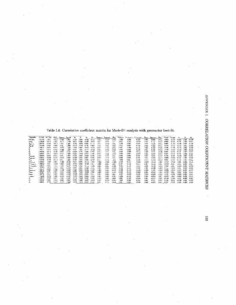
Table 1.4: Correlation coefficient matrix for Mode-Ill analysis with georeactor best-fit.
Parameter
Bin2 29u
Am|[
* B « ™ $g«cue a<j
kb
ko kc
JVrandraul
•^•sndomll
WS L 1
fi"C(a,n) ^ » C { a , n ) , C
F"C{a,a)™0-
R*»tn
$g»fMctO>
ReXmv
£ ™ « o i
^common
tl
fa fa
Global
0.83362 0.58449 0.69702 0.64489 0.99017 0.87614 0.96242 0.96857 0.00429 0.00512 0.04768 0.49349 0.00534 0.49206 0.16774 0.84S61 0.00197 0.66751 0.74148 0.96822 0.96847 0.80661
sin* 20 i 2
1.000 -0.015 0.144 0.044 0.009 0.006 -0.012 -0.011 -0.001 -0.000 -0.009 -0.029 -0.001 0.009 0.006 0.349 -0.001 -0.016 -0.005 -0.223 0.235 -0.799
Amjj)
-0.015 1.000 -0.317 -0.480 0.275 0.229 -0.187 -0.366 -0,001 0.000 -0.010 0.031 -0.003 -0.099 -0.016 0.153 0.000 0.020 0.024 0.006 -0.006 0.012
S g * ™ 0.144 -0.317 1.000 0.481 -0.084 -0.053 0.066 0.116 -0,001 -0.002 0.001 -0.398 0.003 0.279 0.022 -0.135 -0.001 0.009 -0.129 -0.030 0.032 -0.107
*geod lS
0.044 -0.480
0.481 1.000 -0.216 -0.166 0.132 0.289 0.001 0.000 0.006 -0.033 0.002 0.062 0.018 -0.225 -0.001 -0.010 -0.017 -0.011 0.011 -0.035
ao
0.009 0.275 -0.084 -0.216 1.000 0.867 -0,920 -0.924 0.000 -0.000 0.006 0.015 -0.000 0.174 0.069 0.049 0.000 -0.008 -0.009 -0.002 0.002 -0.009
A* 0,006 0,229 -0.053 -0.166 0.867 1.000 -0,771 -0.792 0.000 -0.001 0.015 0.010 0.000 0.149 0.061 0.040 -0.000 -0.006 -0.006 -0,002 0,003 -0.005
fco -0.012 -0.187 0.066 0.132 -0.920 -0.771 1.000 0.747 -0,000 0.001 -0.001 -0.016 -0.000 -0.114 -0.045 -0.034 -0.000 0.001 0.003 0,007 -0.007 0.013
ka
-0.011 -0.366 0.116 0.289 -0.924 -0.792 0.747 1.000 0,000 0.000 -0.007 -0.020 0.000 -0,242 -0.091 -0.067 •.000 0.011 •.013 0.002 -0.002 0,011
NirdriQmi
-0.001 -0.001 -0.001 0,001 0,000 0.000 -0.000 0.000 1.000 0.000 0.001 -0.001 0.000 0.001 0.000 -0.001 0.000 0,000 0,000 -0.000 0.000 0.001
JVrandomll
-0.000 0.000 -0,002 0.000 -0.000 -0.001 0.001 0.000 0.000 1,000
-0.001 -0.002 0.000 0.001 -0.001 -0.001 -0.000 -0.000 -0.000 0.000 -0.000 -0.001
N°u
-0.009 -0.010 0.001 0.006 0.006 0.015 -0.001 -0.007 0.001 -0.001 1,000 -0,004 0.001 -0,006 -G.019 -0,016 -0.000 0.001 -0.001 0.002 -0.000 0.014
R"C(o,n) -0.029 0.031 -0.398 -0.033 0.015 0.010 -0.016 -0.020 -0,001 -0.002 -0.004 1.000 0.001 -0.222 -0,010 -0.008 0.000 -0.017 -0.014 0.002 -0.002 0.01E
^ c , a , n ) , c
-0.001 -0,003 0.003 0.002 -0.000 0.000 -0.000 0.000 0.000 0.000 0.001 0.001 1.000 0.000 0.001 -0.002 0.000 -0.000 -0.001 0.000 0.000 0,001
Rfte&OL 0.009 -0.099 0.279 0.062 0.174 0.149 -0.114 -0.242 0.001 0.001 -0.006 -0.222 0.000 1.000 0,035 -0,156 -0.000 0,023 0,029 -0.005 0.005 -0.006
H ^ t n
0.006 -0.016 0.022 0.018 0.069 0.061 -0.045 -0.091 0.000 -0.001 -0.019 -0.010 0.001 0.035 1.000 -0,086 -0.000 0.014 0.024 0.001 0.000 0.003
_ * a ^ » L 0.349 0.153 -0.135 -0.225 0.049 0.040 -0.034 -0.067 -0.001 -0.001 -0.016 -0.008 -0.002 -0.156 -0.086 1.000 -0.000 -0.430 -0.512 -0.071 0.075 -0.277
K t m ,
-0.001 0.000 -0.001 -0.001 0.000 -0.000 -0.000 0.000 0,000 -0.000 -0.000 0.000 0,000 -0.000 -0.000 -0.000 1.000 -G.000 0.001 0,000 0.000 0.001
e ^ u *
-0.016 0,020 0.009 -0,010 -0.008 -0.006 0,001 0.011 0.000 -0.000 0,001 -0.017 -0.000 0,023 0,014 -0.430 -0.000 1,000 -0.089 -0.002 0.002 0.007
^oramon
-6.005 0.024 -0.129 -0.017 -0,009 -0.006 0.003 0.013 0.000 -0,000 -0.001 -0,014 -0.001 0.029 0.024 -0.512 0.001 -0,089 1.000 -0.002 0.002 0.003
& -0.223 0.006 -0.030 -0.011 -0.002 -0.002 0.007 0.002 -0.000 0,000 0.002 0.002 0.000 -0.005 0.001 -0.071 0.000 -0.002 -0.002 1.000 -0.968 0.283
<fa 0.235 -0.006 0.032 0.011 0.002 0.003 -0.007 -0,002 0.000 -0.000 -0.000 -0.002 0.000 0.005 0.000 0.075 0.000 0.002 0.002 -0.968 1.000
-0.295
A -0.799 0.012 -0,107 -0.035 -0,009 -0.005 0.013 0,011 0,001 -0.001 0.014 0.015 0.001 -0.006 0,003 -0.277 0.001 0.007 0.003 0.283 -0.295 1.000

APPENDIX I. CORRELATION COEFFICIENT MATRICES 194

»., «.
Bibliography
[1] W. Pauli, Letter to the physical society of Tubingen, Unpublished., 1930.
[2] L. M. Brown, Phys. Today 31N9 (1978).
[3] E. Fermi, Z. Phys. 88, 161 (1934).
[4] F. Reines and C. L. Cowan, Phys. Rev. 92, 830 (1953).
[5] C. L. Cowan, F. Reines, F. B. Harrison, H. W. Kruse, and A. D. McGuire,
Science 124, 103 (1956).
[6] J. Davis, Raymond, D. S. Harmer, and K. C. Hoffman, Phys. Rev. Lett. 20,
1205 (1968).
[7] G. Danby et al, Phys. Rev. Lett. 9, 36 (1962).
[8] M. L. Perl et al, Phys. Rev. Lett. 35, 1489 (1975).
[9] DONUT, K. Kodama et al, Phys. Lett. B504, 218 (2001), hep-ex/0012035.
[10] J. N. Bahcall, N. A. Bahcall, and G. Shaviv, Phys. Rev. Lett. 20, 1209 (1968).
[11] D. N. Abdurashitov et al, Phys. Lett. B328, 234 (1994).
[12] GALLEX, W. Hampel et al, Phys. Lett. B447, 127 (1999).
[13] K. S. Hirata et al, Phys. Rev. Lett. 65, 1297 (1990).
[14] Y. Fukuda et al, Phys. Rev. Lett. 81, 1158 (1998).
195
BIBLIOGRAPHY 196
[15] R. Becker-Szendy et al, Phys. Rev. D 46, 3720 (1992).
[16] Kamiokande-II, K. S. Hirata et al, Phys. Lett. B280, 146 (1992).
[17] Z. Maki, M. Nakagawa, and S. Sakata, Prog. Theor. Phys. 28, 870 (1962).
[18] Q. R. Ahmad et al, Phys. Rev. Lett. 89, 011301 (2002).
[19] SNO, S. N. Ahmed et al, Phys. Rev. Lett. 92, 181301 (2004), nucl-ex/0309004.
[20] Super-Kamiokande, Y. Ashie et al, Phys. Rev. Lett. 93, 101801 (2004), hep-
ex/0404034.
[21] CHOOZ, M. Apollonio et al, Phys. Lett. B466, 415 (1999), hep-ex/9907037.
[22] R. D. McKeown and P. Vogel, Phys. Rept. 394, 315 (2004), hep-ph/0402025.
[23] K. Schreckenbach, G. Colvin, W. Gelletly, and F. Von Feilitzsch, Phys. Lett.
B160, 325 (1985).
[24] P. Vogel, G. K. Schenter, F. M. Mann, and R. E. Schenter, Phys. Rev. C 24,
1543 (1981).
[25] A. A. Hahn et al, Phys. Lett. B218, 365 (1989).
[26] C. Bemporad, G. Gratta, and P. Vogel, Rev. Mod. Phys. 74, 297 (2002).
[27] N. R. Tolich, Experimental study of terrestrial electron anti-neutrinos with Kam-
LAND, PhD thesis, Stanford University, 2005, UMI-31-62346.
[28] S. Enomoto, Neutrino geophysics and observation of geo-neutrinos at Kam-
LAND, PhD thesis, Tohoku University, 2005.
[29] F. Mantovani, L. Carmignani, G. Fiorentini, and M. Lissia, Phys. Rev. D69,
013001 (2004), hep-ph/0309013.
[30] A. M. Dziewonski and D. L. Anderson, Phys. Earth Planet. Interiors 25, 297
(1981).

BIBLIOGRAPHY 197
[31] A. A. Krernenetsky and L. N. Ovchinnikov, Precambrian Res. 33, 11 (1986).
[32] E. Anders and N. Grevesse, Geochim. Cosmochim. Acta 53, 197 (1989).
[33] W. F. McDonough and S. s. Sun, Chem. Geol. 120, 223 (1995).
[34] A. Rocholl and K. P. Jochum, Earth Planet. Sci. Lett. 117, 265 (1993).
[35] H. N. Pollack, S. J. Hurter, and J. R. Johnson, Rev. Geophys. 31, 267 (1993).
[36] A. M. Hofmeister and R. E. Criss, Tectonophysics 395, 159 (2005).
[37] F. M. Richter, Earth Planet. Sci. Lett. 68, 471 (1984).
[38] M. J. Jackson and H. N. Pollack, J. Geophys. Res. 89, 10103 (1984).
[39] T. Spohn and G. Schubert, J. Geophys. Res. 87, 4682 (1982).
[40] O. E. Mogensen and F. M. Jacobsen, Chemical Physics 73, 223 (1982).
[41] P. Vogel and J. F. Beacom, Phys. Rev. D60, 053003 (1999), hep-ph/9903554.
[42] A. Kurylov, M. J. Ramsey-Musolf, and P. Vogel, Phys. Rev. C67, 035502 (2003),
hep-ph/0211306.
[43] KamLAND, K. Eguchi et ai, Phys. Rev. Lett. 90, 021802 (2003), hep-
ex/0212021.
[44] KamLAND, T. Araki et ai, Phys. Rev. Lett. 94, 081801 (2005), hep-ex/0406035.
[45] T. Araki et al, Nature 436, 499 (2005).
[46] J. B. Benziger et ai, Nucl. Instrum. Meth. A417, 278 (1998).
[47] F. Suekane et ai, (2004), physics/0404071.
[48] A. D. Vijaya and A. Kumar, Nucl. Instrum. Meth. I l l , 435 (1973).
BIBLIOGRAPHY 198
[49;
[50
[51
[52;
[53;
[54
[55;
[56
[57;
[58
[59
[60
[61
[62;
W. H. Press, B. P. Flannery, S. A. Teukolsky, and W. T. Vetterling, Numerical
Recipes in C: The Art of Scientific Computing (Cambridge University Press,
Cambridge, 1992).
D. Dwyer, Precision Measurement of Neutrino Oscillation Parameters with Kam-
LAND, PhD thesis, University of California, Berkeley, 2007.
B. K. Fujikawa, Quenching and Cerenkov corrections to the KamLAND energy
scale, KamLAND collaboration internal document. Unpublished., 2003.
J. B. Birks, The theory and practice of scintillation counting Vol. 27, Interna
tional series of monographs on electronics and instrumentation (Macmillian, New
York, 1964).
J. D. Jackson, Classical Electrodynamics (Wiley, New York, 1990).
T. Hagner et al, Astropart. Phys. 14, 33 (2000).
D. R. Tilley et al., Nucl. Phys. A 745, 155 (2004).
T. R. England and B. F. Rider, 1994, LA-UP-94-3106, ENDF-349.
http://wwwndc.tokai-sc.jaea.go.jp/ftpnd/jendl/jendl-an-2003.html.
http://www.srim.org/.
D. West and A. C. Sherwood, Ann. Nucl. Energy 9, 551 (1982).
D. A. Dwyer and R. McKeown, Calculation of atmospheric neutrino background
in Kamland, KamLAND collaboration internal document. Unpublished., 2007.
L. A. Ahrens et al, Phys. Rev. D35, 785 (1987).
M. Honda, T. Kajita, K. Kasahara, S. Midorikawa, and T. Sanuki, Phys. Rev.
D75, 043006 (2007), astro-ph/0611418.
[63] J. N. Bahcall, A. M. Serenelli, and S. Basu, Astrophys. J. 621, L85 (2005),
astro-ph/0412440.
BIBLIOGRAPHY 199
[64] SNO, B. Aharmim et al, Phys. Rev. C72, 055502 (2005), nucl-ex/0502021.
[65] Super-Kamkiokande, J. Hosaka et al, Phys. Rev. D73, 112001 (2006), hep-
ex/0508053.
[66] B. T. Cleveland et al, Astrophys. J. 496, 505 (1998).
[67] SAGE, V. N. Gavrin, Nucl. Phys. Proc. Suppl. 138, 87 (2005).
[68] GNO, M. Altmann et al, Phys. Lett. B616, 174 (2005), hep-ex/0504037.
[69] R. G. H. Robertson, Prog. Part. Nucl. Phys. 57, 90 (2006), nucl-ex/0602005.
[70] J. N. Bahcall and M. H. Pinsonneault, Phys. Rev. Lett. 92, 121301 (2004),
astro-ph/0402114.
[71] J. N. Bahcall and M. H. Pinsonneault, Rev. Mod. Phys. 67, 781 (1995), hep-
ph/9505425.
[72] A. Stuart et al, Kendall's Advanced Theory of Statistics Vol. 2A (Oxford Uni
versity Press, New York, 1999).
[73] J. M. Herndon, Proc. Nat. Acad. Sci. 100, 3047 (2003).
[74] J. M. Herndon and D. A. Edgerley, (2005), hep-ph/0501216.