Measurement of Material Nonlinearity using Laser Ultrasound
167
Measurement of Material Nonlinearity using Laser Ultrasound by Ian J Collison, MEng Thesis submitted to the University of Nottingham for the degree of Doctor of Philosophy, July 2008
Transcript of Measurement of Material Nonlinearity using Laser Ultrasound

Measurement of Material Nonlinearity
using Laser Ultrasound
by Ian J Collison, MEng
Thesis submitted to the University of Nottingham
for the degree of Doctor of Philosophy, July 2008

Abstract
The aim of the work in this thesis was to develop an NDT technique capable of
measuring velocity changes caused by an applied stress.
A dual frequency mixing technique was used to perform the experiments, in which
the interaction between two surface acoustic waves (SAWs) was observed. The pump
SAW, generated by a transducer, stressed the sample surface. The probe SAW was
generated by an Optical Scanning Acoustic Microscope (OSAM), capable of gener-
ating ultrasound at 82MHz and its harmonics. The level of stress experienced by
the probe SAW was adjusted by controlling the pump-probe interaction-point using
a system of timing electronics. The nonlinear interaction was directly measured as
a phase modulation of the probe SAW and equated to a velocity change. Detection
of both SAWs was achieved using a knife-edge detector. The stresses exerted by the
transducer were typically <10MPa and the velocity-stress relationship provided a
measure of material nonlinearity.
The technique described herein was sensitive to changes in temperature and,
therefore, several temperature suppression techniques were developed to improve
acquisition of results. CHeap Optical Transducers (CHOTs) were integrated into
the experiment and the measurements obtained using these devices were similar to
those acquired using the knife-edge detector.
Velocity changes of 115.2mms−1/MPa, −34.4mms−1/MPa and −31.9mms−1/MPa
were measured on fused silica, Al-2024 and Al-6061, respectively. Experiments
showed that fused silica and aluminium had opposite nonlinear responses, consistent
with previous published data. The work in this thesis could be applied to fatigue
measurements, for example in the aeronautics industry, to safely and reliably extend
the useable life of aircraft engine components.

Acknowledgements
I would first of all like to thank my supervisor Dr M Clark for all of his guidance,
support and suggestions throughout this research. Thanks go to Professor M Somekh
for his advice and assistance and also to Dr S Sharples who has always been willing to
advise. I also express my gratitude to Teti Stratoudaki for our endless, yet enjoyable,
discussions and for her encouragement. Thanks go to Jose Hernandez and to my
other colleagues: Richard Smith, Robert Ellwood and Wen-qi Li.
My appreciation also goes to the technicians at Nottingham University for al-
lowing me to use their facilities and to Brian Webster for providing his expertise
on sample preparation and allowing me to perform experiments on the fatiguing
machines in the Mechanical Engineering Department. In addition, I thank Katy
Milne and the technicians at Rolls-Royce for their help with fatiguing samples.
My gratitude must also extend to my family and friends for their continued
support and encouragement.
Contents
1 Introduction 1
1.1 Objective and outline of thesis . . . . . . . . . . . . . . . . . . . . . . 1
1.2 The need for NDT . . . . . . . . . . . . . . . . . . . . . . . . . . . . 4
1.3 NDT techniques currently used in industry . . . . . . . . . . . . . . . 5
1.4 Ultrasound . . . . . . . . . . . . . . . . . . . . . . . . . . . . . . . . . 6
1.4.1 Bulk waves . . . . . . . . . . . . . . . . . . . . . . . . . . . . 7
1.4.2 Rayleigh waves . . . . . . . . . . . . . . . . . . . . . . . . . . 8
1.4.3 Lamb waves . . . . . . . . . . . . . . . . . . . . . . . . . . . . 13
1.5 Ultrasound generation and detection using contact devices . . . . . . 14
1.5.1 Transducers . . . . . . . . . . . . . . . . . . . . . . . . . . . . 14
1.5.2 EMATs . . . . . . . . . . . . . . . . . . . . . . . . . . . . . . 16
1.5.3 SAW devices . . . . . . . . . . . . . . . . . . . . . . . . . . . 17
1.5.4 Comb transducers . . . . . . . . . . . . . . . . . . . . . . . . . 17
1.6 Generating ultrasound with lasers . . . . . . . . . . . . . . . . . . . . 18
1.6.1 Review of laser generation techniques . . . . . . . . . . . . . . 20
1.6.2 The g-CHOT . . . . . . . . . . . . . . . . . . . . . . . . . . . 22
1.7 Detecting ultrasound with lasers . . . . . . . . . . . . . . . . . . . . . 23
1.7.1 Knife-edge detection . . . . . . . . . . . . . . . . . . . . . . . 23
1.7.2 Interferometry . . . . . . . . . . . . . . . . . . . . . . . . . . . 24
1.7.3 The d-CHOT . . . . . . . . . . . . . . . . . . . . . . . . . . . 26
i
CONTENTS ii
1.8 Summary . . . . . . . . . . . . . . . . . . . . . . . . . . . . . . . . . 28
2 Literature Review 29
2.1 Introduction . . . . . . . . . . . . . . . . . . . . . . . . . . . . . . . . 29
2.2 Linear elasticity . . . . . . . . . . . . . . . . . . . . . . . . . . . . . . 30
2.3 Nonlinear experimental techniques . . . . . . . . . . . . . . . . . . . . 33
2.3.1 Higher harmonic generation − ‘self-stressing’ method . . . . . 33
2.3.2 Parametric interaction . . . . . . . . . . . . . . . . . . . . . . 35
2.3.3 Nonlinear-time reversal acoustics (NL-TRA) . . . . . . . . . . 37
2.3.4 Nonlinear reverberation spectroscopy (NRS) . . . . . . . . . . 37
2.4 Summary . . . . . . . . . . . . . . . . . . . . . . . . . . . . . . . . . 38
3 Instrumentation 40
3.1 Introduction . . . . . . . . . . . . . . . . . . . . . . . . . . . . . . . . 40
3.2 Optical setup for the generation of ultrasound . . . . . . . . . . . . . 40
3.2.1 Generation source . . . . . . . . . . . . . . . . . . . . . . . . . 42
3.2.2 Beam expansion . . . . . . . . . . . . . . . . . . . . . . . . . . 44
3.2.3 Beam manipulation . . . . . . . . . . . . . . . . . . . . . . . . 45
3.2.4 SLM . . . . . . . . . . . . . . . . . . . . . . . . . . . . . . . . 46
3.2.5 Camera system . . . . . . . . . . . . . . . . . . . . . . . . . . 48
3.3 Knife-edge detector . . . . . . . . . . . . . . . . . . . . . . . . . . . . 49
3.3.1 Optical configuration . . . . . . . . . . . . . . . . . . . . . . . 49
3.3.2 Electronic configuration . . . . . . . . . . . . . . . . . . . . . 51
3.3.3 Calibrating the detector system . . . . . . . . . . . . . . . . . 56
3.4 CHOT system configuration . . . . . . . . . . . . . . . . . . . . . . . 63
3.4.1 g-CHOT . . . . . . . . . . . . . . . . . . . . . . . . . . . . . . 63
3.4.2 d-CHOT . . . . . . . . . . . . . . . . . . . . . . . . . . . . . . 67
3.5 High-speed data acquisition − the analogue electronics . . . . . . . . 69

CONTENTS iii
3.6 Summary . . . . . . . . . . . . . . . . . . . . . . . . . . . . . . . . . 71
4 Experimental Method 72
4.1 Introduction . . . . . . . . . . . . . . . . . . . . . . . . . . . . . . . . 72
4.2 Experimental aim and concept . . . . . . . . . . . . . . . . . . . . . . 73
4.3 Nonlinear experiment configuration . . . . . . . . . . . . . . . . . . . 74
4.3.1 Pump SAW generation . . . . . . . . . . . . . . . . . . . . . . 76
4.3.2 Timing setup . . . . . . . . . . . . . . . . . . . . . . . . . . . 77
4.3.3 Experimental timing error . . . . . . . . . . . . . . . . . . . . 79
4.3.4 Materials and sample preparation . . . . . . . . . . . . . . . . 82
4.4 Nonlinear/CHOT experiment configuration . . . . . . . . . . . . . . . 82
4.5 The effects of temperature . . . . . . . . . . . . . . . . . . . . . . . . 84
4.6 Suppressing temperature dependence . . . . . . . . . . . . . . . . . . 87
4.6.1 Temperature control system . . . . . . . . . . . . . . . . . . . 87
4.6.2 Differential data acquisition . . . . . . . . . . . . . . . . . . . 92
4.6.3 Interlacing differential data acquisition . . . . . . . . . . . . . 93
4.6.4 Interlacing differential data acquisition with temperature control 98
4.7 Comparison of temperature suppression techniques . . . . . . . . . . 100
4.8 Summary . . . . . . . . . . . . . . . . . . . . . . . . . . . . . . . . . 101
5 Experimental Results 103
5.1 Introduction . . . . . . . . . . . . . . . . . . . . . . . . . . . . . . . . 103
5.2 Extracting the phase . . . . . . . . . . . . . . . . . . . . . . . . . . . 104
5.3 Validation of nonlinear measurement − the ‘anti-propagating’ test . . 104
5.4 Changing the pump SAW amplitude . . . . . . . . . . . . . . . . . . 107
5.4.1 Selecting appropriate delay settings . . . . . . . . . . . . . . . 109
5.4.2 Experimental procedure and results . . . . . . . . . . . . . . . 111
5.5 Changing the pump SAW frequency . . . . . . . . . . . . . . . . . . . 115

CONTENTS iv
5.6 Changing the probe SAW frequency . . . . . . . . . . . . . . . . . . . 120
5.7 Comparison of nonlinear responses of fused silica and aluminium . . . 126
5.8 Nonlinear experiments with CHOTs . . . . . . . . . . . . . . . . . . . 131
5.9 Summary . . . . . . . . . . . . . . . . . . . . . . . . . . . . . . . . . 135
6 Conclusion and further work 138
Appendix A: Material Properties 141
Appendix B: Brief history of the OSAM Instrument 142
Appendix C: OSAM Alignment 144
Introduction . . . . . . . . . . . . . . . . . . . . . . . . . . . . . . . . . . . 144
Laser cavity . . . . . . . . . . . . . . . . . . . . . . . . . . . . . . . . . . . 144
SLM and surrounding optics . . . . . . . . . . . . . . . . . . . . . . . . . . 145
Sample . . . . . . . . . . . . . . . . . . . . . . . . . . . . . . . . . . . . . . 145
Bibliography 148

Chapter 1
Introduction
1.1 Objective and outline of thesis
The work in this thesis was based on the development of a sensitive, robust and
repeatable nondestructive testing (NDT) technique capable of measuring velocity
changes caused by applied stress. The velocity-stress relationship is a direct mea-
surement of material nonlinearity.
The motivation for this work was to investigate the changes in material nonlin-
earity caused by fatigue. From a material-science perspective, this technique is an
extremely powerful tool for accurate material qualification and can be applied to
many areas of industry, such as the aerospace industry for example.
The experiments used a dual frequency mixing technique in which the inter-
action between two surface acoustic waves (SAWs) was observed. A low frequency
(500kHz−2MHz) pump SAW was generated by a transducer, which stressed the sur-
face of the sample as it propagated. The high frequency (82MHz, 164MHz, 246MHz)
probing SAW, was generated by the Optical Scanning Acoustic Microscope (OSAM)
instrument [1].
By altering the point of interaction between the two SAWs, the stress experi-
enced by the probe was controlled, and a change in velocity was directly measured
1
CHAPTER 1. INTRODUCTION 2
in the phase of the high frequency probe SAW. Ultrasound detection was performed
by a knife-edge detector. In addition, the application of CHOTs provided an alter-
native method to generate and detect ultrasound. The advantage of performing this
experiment with lasers was that the experiment was non-contact. Moreover, the
benefits of generating and detecting ultrasound with lasers include a higher spatial
resolution compared with contact methods and the ability to perform couplant-free
experiments.
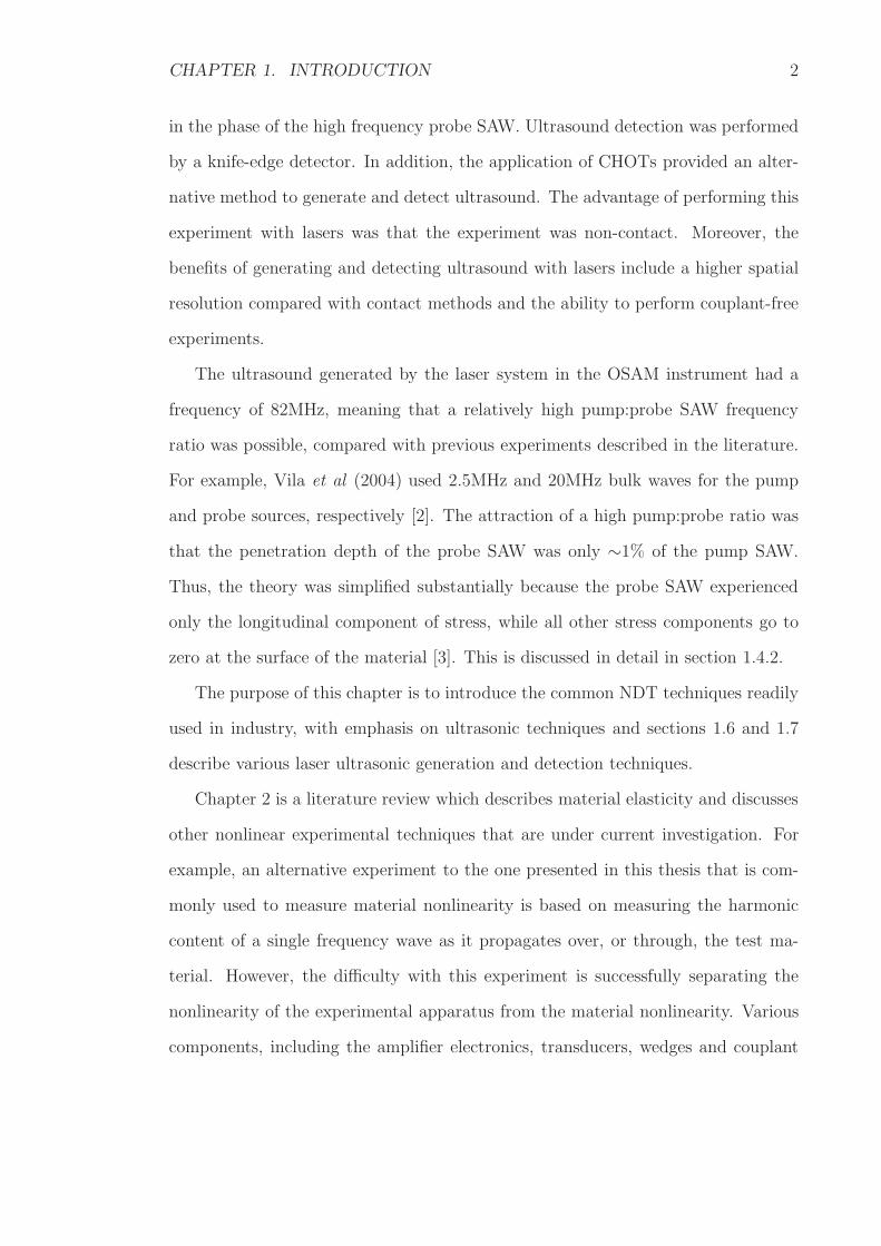
The ultrasound generated by the laser system in the OSAM instrument had a
frequency of 82MHz, meaning that a relatively high pump:probe SAW frequency
ratio was possible, compared with previous experiments described in the literature.
For example, Vila et al (2004) used 2.5MHz and 20MHz bulk waves for the pump
and probe sources, respectively [2]. The attraction of a high pump:probe ratio was
that the penetration depth of the probe SAW was only ∼1% of the pump SAW.
Thus, the theory was simplified substantially because the probe SAW experienced
only the longitudinal component of stress, while all other stress components go to
zero at the surface of the material [3]. This is discussed in detail in section 1.4.2.
The purpose of this chapter is to introduce the common NDT techniques readily
used in industry, with emphasis on ultrasonic techniques and sections 1.6 and 1.7
describe various laser ultrasonic generation and detection techniques.
Chapter 2 is a literature review which describes material elasticity and discusses
other nonlinear experimental techniques that are under current investigation. For
example, an alternative experiment to the one presented in this thesis that is com-
monly used to measure material nonlinearity is based on measuring the harmonic
content of a single frequency wave as it propagates over, or through, the test ma-
terial. However, the difficulty with this experiment is successfully separating the
nonlinearity of the experimental apparatus from the material nonlinearity. Various
components, including the amplifier electronics, transducers, wedges and couplant

CHAPTER 1. INTRODUCTION 3
all contribute to some degree to the measured harmonic content, and, therefore,
these must be accounted for. The technique presented in this work is immune to
this problem because the inter-modulation of two independent SAWs was being
measured.
Chapter 3 describes the OSAMs optical setup for the generation and detection
of ultrasound, as well as the detector electronics and calibration scheme. During the
course of this work, it was found that the stress-related velocity-change measure-
ments were affected by changes in temperature. Various methods were developed to
suppress the temperature effect which are presented in Chapter 4.
The generation laser system in the OSAM is capable of generating SAWs at
a fundamental frequency of 82MHz, as well as at the harmonics. Therefore, in
addition to using the fundamental frequency, the nonlinear experiment could also
be performed using frequencies of 164MHz and 246MHz, as demonstrated in Chapter
5.
The materials that were investigated in this work were fused silica and alu-
minium. These materials were selected because they have a relatively high nonlin-
earity property [4], compared with other materials (e.g. steel, gold, titanium, copper
and silver) making them most appropriate for the development of a nonlinear ex-
periment.
In the literature, the material nonlinearity is often quantified using the β (‘nonlin-
ear’) parameter. Although it is possible to quantify the fatigue level of a material by
measuring changes in β, material nonlinearity was not measured using this method
in the work presented here. Instead, the relationship between velocity change and
stress provided the quantitative measure of nonlinearity. This can be referred to as a
measurement of acoustoelasticity i.e the stress dependence of acoustic wave velocity
in elastic media [5].
According to the literature, fused silica and aluminium are reported to have op-

CHAPTER 1. INTRODUCTION 4
posite nonlinear responses [4]. In order to validate this experiments were performed
on these materials and the results are presented in Chapter 5.
In parallel with the nonlinear research, the Applied Optics Group (AOG) at the
University of Nottingham has been developing CHeap Optical Transducer (CHOT)
technology. These devices are activated by lasers and can generate and detect ul-
trasound with the generation-CHOT (g-CHOT) and detection-CHOT (d-CHOT),
respectively. The advantage of a CHOT-nonlinear system was that the optical setup
could simplified. CHOTs were applied to the nonlinear experiment and the results
are presented in Chapter 5. Finally, Chapter 6 will summarise the work, discuss
improvements, limitations and possible improvements, and describe the future of
the experiment for NDT applications.
1.2 The need for NDT
Nondestructive testing (NDT) is the process through which material is tested for
abnormalities and defects without causing any damage to it i.e. to evaluate an
object’s integrity without changing it in any way. This process may also be referred
to as nondestructive inspection (NDI) or nondestructive evaluation (NDE).
NDT is essential in many industrial sectors such as the aerospace, nuclear, and
pipeline industries. Ultimately, the motivation behind NDT is to provide reliable
products by minimising the risk of failure thereby reducing costs and maximising
safety. NDT is used to characterise materials, monitor manufacturing processes and
detect defects.
Defects are caused by many manufacturing processes such as melting, grinding,
welding and joining. It is important that NDT is applied at various stages of manu-
facture to demonstrate that a component continues to meet a specific standard and
that the material has not been weakened by the manufacturing processes.
The application of NDT during component testing provides useful information
CHAPTER 1. INTRODUCTION 5
about the presence and growth of defects, which can then be used to make ‘life-time’
predictions. Once in service, factors such as over-loading the component, fatigue and
corrosion can cause further defects and, therefore, ‘in-service’ inspection is vital so
that components can be repaired or replaced, if necessary.
The down-time required for this kind of inspection is usually minimised to reduce
costs and particularly for the aerospace industry, often leads to ‘on-wing’ inspection.
Developing NDT techniques that can be performed quickly, efficiently and in difficult
to reach places is challenging but has obvious benefits.
In the aerospace industry, there is momentum towards lighter and more efficient
engines, driven by attempts to reduce the cost of flying. To reduce weight, new
materials such as carbon composites and metal matrix composites (MMCs) are
being developed. Before they can be put into service, it is essential that the risks
involved are managed − NDT forms an essential part of managing these risks.
With the introduction of new materials comes the potential requirement for new
NDT techniques. In addition, there is a demand for inspection methods that can
provide earlier indications of material failure than present techniques and, thus,
provides a strong rationale for the work presented in this thesis.
1.3 NDT techniques currently used in industry
The most widely used NDT methods in industry include visual inspection, pene-
trant testing, magnetic particle inspection (MPI), eddy current inspection (ECT),
radiography and ultrasound. Selection of the most appropriate method is based on
the material type, defect size and location, and accessibility.
Visual inspection involves chemically etching or electro-chemically etching the
component, so that the surface condition can be examined. Variations in grain size,
inclusions, grinding abuse, cracks and folds can be identified using this method. Al-
though it is a simple and fairly rapid method, it is limited only to surface inspection.

CHAPTER 1. INTRODUCTION 6
Liquid penetrant testing (LPI) involves coating the component with a liquid
penetrant, which will enter into any surface cracks. Subsequently, excess penetrant
is removed and a developer is applied. The developer ‘draws’ out the penetrant that
remains in the crack making it visible. Although this is an inexpensive and simple
method it is relatively slow and limited to non-porus materials.
MPI is limited to surface inspection of ferromagnetic materials. It is based on
detecting changes in the magnetic permeability of ferromagnetic materials, due to
the presence of flaws. However, it is only sensitive to flaws that are transverse to
the magnetic field being applied to the material.
ECT inspection is limited to inspecting cracks near the surface of conductive
samples. It is unable to examine large-areas but it is still very popular in industry
because it is portable and provides immediate test results.
Inspecting with radiography consists of using X-rays to penetrate the surface
of the sample. The radiation emerging from the opposite side of the material can
then be detected and used to determine the location and presence of flaws inside the
sample. It can be applied to all materials with any surface condition and no couplant
is required. However, it is expensive and requires access to the opposite side of the
object under investigation, which is not always possible or straight-forward.
1.4 Ultrasound
The role of ultrasonics within the NDT community has increased dramatically over
the last 30 years. At present, industrial ultrasonic inspection techniques use contact
transducers for through-transmission and pulse-echo measurements, but there is a
potential for further ultrasonic methods to be exploited, such as non-contact and
nonlinear techniques.
Sounds that have a frequency above the audible human range (20Hz−20kHz) are
termed ultrasonic. Ultrasound is useful because it allows media to be non-invasively

CHAPTER 1. INTRODUCTION 7
inspected. Many people are familiar with its application to the medical industry
and its ability to ‘see’ inside the human body. The fact that it provides information
about the inside of an object makes it a very important technique, suitable for a
wide range of applications.
When applied to NDT, the ultrasonic wave frequency and mode is selected de-
pending on factors, such as material type, geometry, defect size, shape, orientation
and location. The following sections briefly describe the most commonly used wave
modes that are used for ultrasonic inspection.
1.4.1 Bulk waves
In an isotropic solid, there are two distinct bulk wave modes − the longitudinal and
transverse modes. The longitudinal wave mode causes the particles in the solid to
vibrate parallel to the direction of wave propagation. Waves that have this form of
vibration can also be called compressional, pressure or density waves. The other is
the transverse or shear mode, which causes the particles to oscillate at right angles
to the direction of wave propagation. Figure 1.1 compares the particle movement
for the two modes.
Sz Syz
x
yWave propagation
Lx
Sample
Figure 1.1: Particle displacement for the propagating longitudinal (L) and shear (S)modes. Particle L has motion in the x direction, while particle S experiences motionin the y and z directions.
Bulk waves are used to detect defects located within the material and are often
generated and detected using contact transducers (see section 1.5.1). The probability
CHAPTER 1. INTRODUCTION 8
of detection (POD) is increased by using a number of transducers, which excite
bulk waves at different angles. This is because the reflected (or transmitted) sound
depends on the orientation of the defect with respect to the propagating ultrasound.
1.4.2 Rayleigh waves
The use of ultrasound to detect the presence of defects is not limited to the interior
of materials. Defects located on or near the surface of materials are more effectively
detected using surface waves than bulk waves. This is because the minimum distance
between the defect and the surface is related to the pulse duration of the transducer.
The type of surface wave that is of interest to the NDT community is the Rayleigh
wave [6]. The penetration depth of Rayleigh waves is approximately equal to their
wavelength, which makes them suitable for inspecting the near-surface of materials.
During the 1950s, investigators began using Rayleigh waves for material inspection
in the laboratory [7, 8]. Following these early investigators, Rayleigh wave ‘visu-
alisation’ techniques based on optical scanning detection systems were successfully
developed [9, 10].
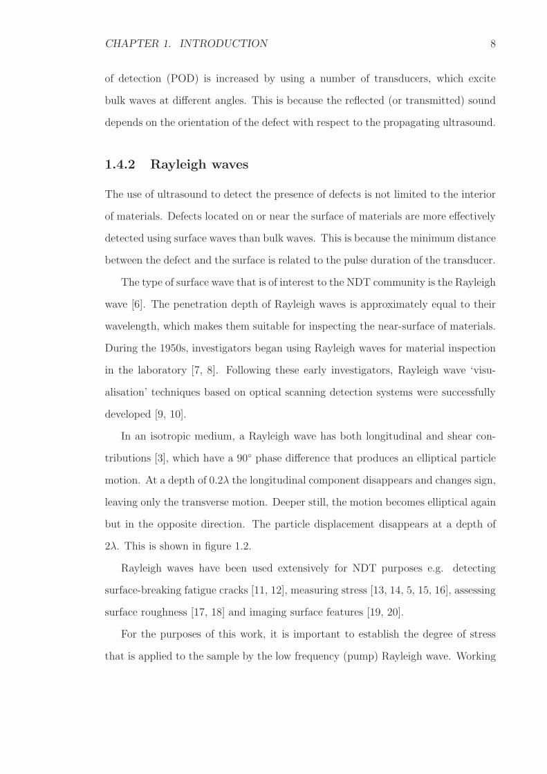
In an isotropic medium, a Rayleigh wave has both longitudinal and shear con-
tributions [3], which have a 90 phase difference that produces an elliptical particle
motion. At a depth of 0.2λ the longitudinal component disappears and changes sign,
leaving only the transverse motion. Deeper still, the motion becomes elliptical again
but in the opposite direction. The particle displacement disappears at a depth of
2λ. This is shown in figure 1.2.
Rayleigh waves have been used extensively for NDT purposes e.g. detecting
surface-breaking fatigue cracks [11, 12], measuring stress [13, 14, 5, 15, 16], assessing
surface roughness [17, 18] and imaging surface features [19, 20].
For the purposes of this work, it is important to establish the degree of stress
that is applied to the sample by the low frequency (pump) Rayleigh wave. Working
CHAPTER 1. INTRODUCTION 9
00.2
0.40.6
0.81
1.2−0.2 0
0.2
0.4
0.6
0.8 1
1.2
z/λ
U
Uz
x
0.2λ
λz
y
x
z
Wave propagation
(a) (b)
−0.2 0 0.2 0.4 0.6 0.8 1.0
Normalised displacement
0
0.2
0.4
0.6
0.8
1.0
1.2
Figure 1.2: Normalised displacements (Ux and Uz) in the x and z directions (a).Particle motion caused by a propagating Rayleigh wave in the positive x direction(b). Both (a) and (b) were produced by the author using the theory explained inthe latter part of this section.
from [3], the particle displacements along the x and z axes of figure 1.2 are written
as follows:
Ux =∂ϕ
∂x−∂ψ
∂z(1.1)
Uz =∂ϕ
∂z+∂ψ
∂x(1.2)
where ϕ and ψ are the scalar and vector potentials of the displacements given below:
ϕ = Ae−qzei(kx−ωt) (1.3)
ψ = Be−szei(kx−ωt) (1.4)
where A and B are arbitrary constants, k is the wave number, ω is the angular
frequency, and where q and s can be written as:

CHAPTER 1. INTRODUCTION 10
q2 = k2 − k2l (1.5)
s2 = k2 − k2t (1.6)
in which kl and kt are the wave numbers for the longitudinal and transverse modes,
respectively, and are given below:
kl = ω
√
ρ
λ+ 2µ(1.7)
kt = ω
√
ρ
µ(1.8)
where λ and µ are the bulk and shear moduli, respectively, and ρ is the medium
density. The stress components (σxx, σzz and σxz) are also given as:
σxx = λ(∂2ϕ
∂x2+∂2ϕ
∂z2) + 2µ(
∂2ϕ
∂x2+
∂2ψ
∂x∂z) (1.9)
σzz = λ(∂2ϕ
∂x2+∂2ϕ
∂z2) + 2µ(
∂2ϕ
∂z2+
∂2ψ
∂x∂z) (1.10)
σxz = µ(2∂2ϕ
∂x∂z+∂2ψ
∂x2−∂2ψ
∂z2) (1.11)
By substituting equations 1.3 and 1.4 into 1.11 (for example), it is possible to obtain
an expression for B in terms of A as follows:
B = −2Aqik
k2 + s2(1.12)
Also, by using 1.6 with 1.8 and 1.5 with 1.7, an expression for µ and λ, respectively,
is obtained:

CHAPTER 1. INTRODUCTION 11
µ =ω2ρ
k2 − s2(1.13)
λ =ω2ρ((k2 − s2) − 2(k2 − q2))
(k2 − q2)(k2 − s2)(1.14)
By using equations 1.1, 1.2 and 1.12 and taking the real part only, the equations for
the displacements are as follows:
Ux = −Ak(e−qz −2qs
k2 + s2e−sz)sin(kx− ωt) (1.15)
Uz = −Aq(e−qz +2k2
k2 + s2e−sz)cos(kx− ωt) (1.16)
By substituting 1.12, 2.4 and 1.14 into 1.9, 1.10 and 1.11, respectively, similar ex-
pressions are obtained for the stress components, taking the real parts only:
σxx = (λAe−qz(q2 − k2) − 2µAk2(eqz −2qs
k2 + s2e−sz))cos(kx− wt) (1.17)
σzz = (λAe−qz(q2 − k2) + 2µAq(qe−qz −2k2s
k2 + s2e−sz))cos(kx− wt) (1.18)
σxz = −2µAqk(e−sz − e−qz)sin(kx− wt) (1.19)
Using equations 1.17, 1.18 and 1.19, the stresses in a particular material caused
by a Rayleigh wave can be determined.
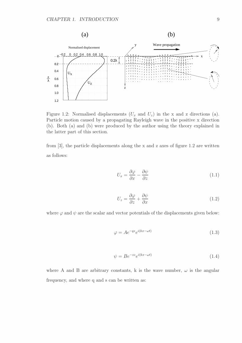
Figure 1.3 shows the normalised stresses. At the surface of the sample, the σzz
and σxz components disappear leaving σxx. For example, if a 1MHz pump SAW
CHAPTER 1. INTRODUCTION 12
0 0.5 1 1.5−0.2
0
0.2
0.4
0.6
0.8
1
1.2
z/λ
Str
ess
(a
rb u
nits
)
σxx
σzz
σxz
Figure 1.3: Rayleigh wave stress components. Here, the data are normalised,whereas in Chapter 5, the same theory was used to ascertain the actual appliedstress on fused silica and aluminium samples using the material properties presentedin Appendix A.
propagates in a material that has a velocity of 3000m/s, the acoustic wavelength
(λLF ) of the SAW is 3mm. A propagating 82MHz probe SAW in the same material
has a wavelength (λHF ) of 36µm. Since λHF≪λLF , it can be assumed that the probe
SAW experiences the stress components at the surface of the sample, i.e. σxx.
From figure 1.2(b), we can see that the longitudinal stress component (σxx) causes
the particles at the peak and trough of the Rayleigh wave to be ‘pulled’ apart and
‘squeezed’ together, respectively. The material is, therefore, experiencing a tensional
stress (+σxx) at the peak and a compressional stress (-σxx) at the trough.
In the elastic region of a ‘linear’ material, the relationship between stress and
strain is constant, which means that the ultrasonic velocity at +σxx and -σxx would
be equal. This is only an approximation because, in a realistic (i.e. ‘non-Hookean’
or ‘nonlinear’) material the stress-strain relationship is nonlinear. In this case, the
induced stress alters the elastic constants of the material, causing subtle changes
in its properties, which can be measured by a change in ultrasonic velocity. How
ultrasonic velocity is affected by applied stress depends on the material type.
CHAPTER 1. INTRODUCTION 13
1.4.3 Lamb waves
Lamb waves are useful for NDT techniques because they have the potential to prop-
agate over considerable distances and, therefore, can be used to inspect large struc-
tures [21]. Research into their interaction with notches [22], delaminations [23] and
cracks [24, 25] has been performed. Non-contact methods of generating and detect-
ing Lamb waves have been previously studied [26, 27].
A Lamb wave travels through the entire thickness of a material, meaning that
both the surfaces and the bulk of the material are interrogated [28]. There are
a number of possible Lamb wave modes, which are often presented in phase (or
group) velocity-dispersion curves. However, two modes that are commonly used are
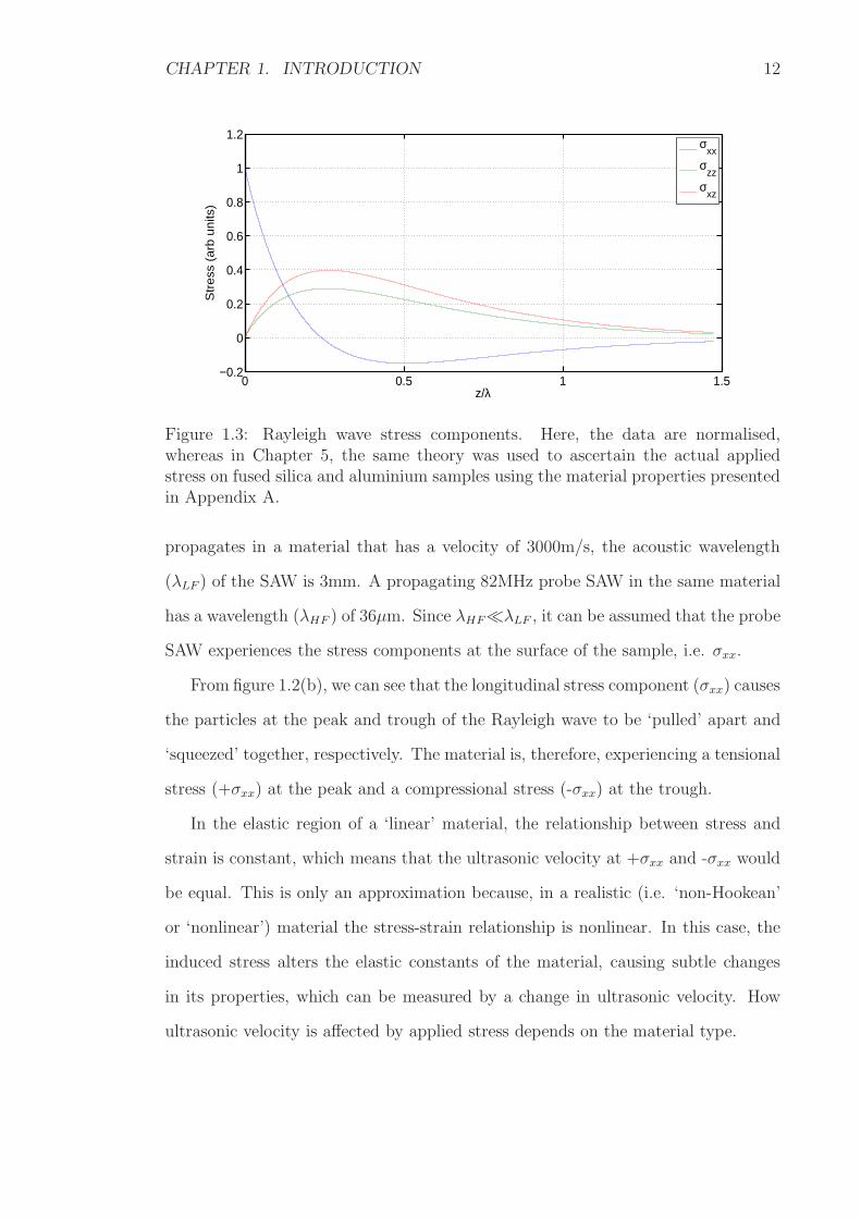
the symmetrical (S0) and asymmetrical (A0) modes. The shapes of these modes are
shown schematically in figure 1.4.
(b)
(a)
Figure 1.4: Schematic diagram of the A0 (a) and S0 (b) modes that are commonlyused in NDT.
In this thesis, the nonlinear experiment was performed on samples that had a
thickness greater than the wavelength of the pump SAW (i.e. with Rayleigh waves).
However, it is also feasible that this experiment will be applied equally well to
relatively thin samples. If the sample thickness is lower than the wavelength of the
pump SAW, then Lamb waves will be excited into the sample. The advantage of
using Lamb waves to stress the surface of the sample is that their point of generation
could potentially be metres away from the point of nonlinear inspection, providing
greater experimental flexibility for difficult to reach areas, for example.

CHAPTER 1. INTRODUCTION 14
1.5 Ultrasound generation and detection using con-
tact devices
Alternative methods exist for generating SAWs other than using a transducer, and
will be reviewed in this section. The advantages and disadvantages of each device
will be discussed.
1.5.1 Transducers
Transducers are a very common method of generating and detecting ultrasound.
They can be used to generate and detect bulk waves or, when attached to a wedge,
excite and detect SAWs.
The active element is made of a piezoelectric or ferroelectric material that when
excited by a time-varying voltage will expand and contract with the applied voltage.
Conversely, if the element is made to expand and contract due to an applied force, a
time-varying voltage output will be generated. A transducer can, therefore, be used
to generate and detect ultrasound.
Transducers are commonly used in two modes of operation: transmit-reflection
(pulse echo) and through-transmission, shown in figure 1.5a and 1.5b respectively.
In transmit-reflection mode, a single transducer is used to excite a bulk wave into
the material. Defects present within the bulk of the material will reflect the sound
back to the source, which the transducer will convert back into a voltage signal. The
time of arrival indicates where the defect is in relation to the sample surface.
Through-transmission requires two transducers − one for generation and the
other for detection. A defect will prevent the wave from propagating through the
material and, therefore, the receiving transducer will not detect the wave.
When used to generate surface waves, the wedge that couples the ultrasound
between the transducer and the sample has to be angled appropriately. The wedge

CHAPTER 1. INTRODUCTION 15
Am
p
Time
Am
p
Time
Reflection from back surfaceReflection from defect
A B
Defect
T/R
B
Am
p
Time
Am
p
Time
T
A
Defect
R
(a) (b)
Figure 1.5: The use of transducers for transmit-reflection (a) and through-transmission (b) to locate a defect.
angle depends on the ratio of ultrasound velocity in the wedge material to that of
the sample material. They are related by Snell’s law, as shown in equation 1.20.
sinθi
vi
=sinθr
vr
(1.20)
Where θi is the incident angle and θr is the angle of refraction from the normal,
as shown in figure 1.6 (to generate a SAW, θr=90). vi and vr are the ultrasound
velocities in the wedge and sample materials, respectively.
θi
θr
Transducer
Wedge
Sample
Figure 1.6: A wedge is used to angle the transducer so that a SAW can be generatedon the surface of the sample.
Polystyrene is the preferred material for transducer wedges because it has a very
low attenuation coefficient (∼0.18dB/mm at 5MHz) [29]. In comparison, PVC has
a higher attenuation factor of 1.12dB/mm at 5MHz [29]. The shape of the wedge
CHAPTER 1. INTRODUCTION 16
is also an important consideration. It has to be designed so that the emitted sound
beam from the transducer is not reflected around the wedge which would otherwise
cause spurious signals.
Attachment of the transducer to the wedge or sample can be achieved in a number
of ways. Liquid couplant such as water or oil can be used as a temporary measure,
but over a period of time, this type of couplant dries out. The alternative is to use
a dry couplant, which bonds the two surfaces together. Phenyl salicylate forms a
solid bond at room temperature but when heated to ∼36 C, melts and the bond
is broken. Once Phenyl salicylate is attached, the measurements are much more
reproducible compared with a liquid-based couplant.
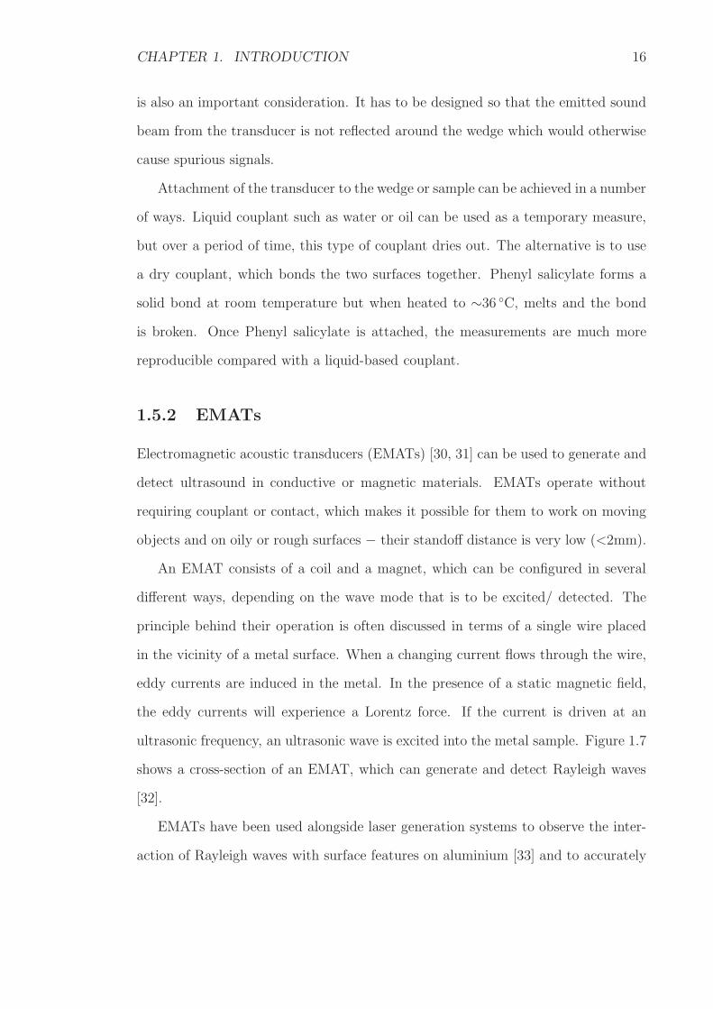
1.5.2 EMATs
Electromagnetic acoustic transducers (EMATs) [30, 31] can be used to generate and
detect ultrasound in conductive or magnetic materials. EMATs operate without
requiring couplant or contact, which makes it possible for them to work on moving
objects and on oily or rough surfaces − their standoff distance is very low (<2mm).
An EMAT consists of a coil and a magnet, which can be configured in several
different ways, depending on the wave mode that is to be excited/ detected. The
principle behind their operation is often discussed in terms of a single wire placed
in the vicinity of a metal surface. When a changing current flows through the wire,
eddy currents are induced in the metal. In the presence of a static magnetic field,
the eddy currents will experience a Lorentz force. If the current is driven at an
ultrasonic frequency, an ultrasonic wave is excited into the metal sample. Figure 1.7
shows a cross-section of an EMAT, which can generate and detect Rayleigh waves
[32].
EMATs have been used alongside laser generation systems to observe the inter-
action of Rayleigh waves with surface features on aluminium [33] and to accurately

CHAPTER 1. INTRODUCTION 17
Sample
N
S
Figure 1.7: Cross-section of an EMAT configuration used to generate and detectRayleigh waves. A ‘meandering’ wire is placed under a magnet and the motion ofthe coil (indicated by the arrows) induces an ultrasonic wave into the sample.
monitor the thickness of an aluminium plate [31, 34].
1.5.3 SAW devices
A section on SAW devices has been included in this chapter because they are anal-
ogous to CHOTs (see sections 1.6.2 and 1.7.3). Conceptually, SAW devices and
CHOTs are very similar. However, the fundamental difference is that CHOTs are
optically activated, giving them the advantage of being non-contact; in contrast,
SAW devices have to be physically connected to external electronics.
Figure 1.8 shows the structure of a SAW device [35]. It consists of two interleaved
sets of ‘fingers’ which are spaced to match the acoustic wavelength of the ultrasound
to be generated. The fingers are metal electrodes that have been deposited on a
piezoelectric substrate such as quartz. By applying an alternating voltage across
the two sets of fingers, at an appropriate frequency, the surface of the piezoelectric
material expands and contracts accordingly. This gives rise to a generated SAW on
the surface of the attached sample. The SAW can be detected by a similar device
commonly operating between a 10MHz−1GHz frequency range.
1.5.4 Comb transducers
A comb transducer (sometimes referred to as the Sokolinskii comb device) uses a
specifically designed wedge, consisting of a comb-like structure, to excite SAWs

CHAPTER 1. INTRODUCTION 18
λ λλ
Sample
SAWGeneration Detection
Figure 1.8: A SAW device is placed onto the surface of a sample and is used togenerate and detect SAWs at a frequency determined by the finger separation.
onto a sample [3]. The teeth of the comb are periodically separated by a distance
equivalent to the acoustic wavelength of the SAW to be generated. Figure 1.9
shows the structure of the device that is bonded to the sample. A transducer is
placed on the upper surface of the wedge for activation of the ultrasound. Comb
transducers have been used to excite Rayleigh waves on aluminium samples for
nonlinear experiments [36].
Piezoelectric transducer
Propagating SAW
λ Comb wedge
Figure 1.9: Structure of a comb transducer. In this case a SAW propagates in bothdirections. If a series of arcs is machined into the wedge, the SAW will propagatein a particular direction.
1.6 Generating ultrasound with lasers
Except for EMATs, all the techniques discussed in previous sections have a disadvan-
tage in that they are all contact methods. The disadvantage with contact techniques
is that they require couplant, which can dry out and become less effective over time.
Contact devices load the sample surface and, therefore, influence the propagation of
ultrasound.
The advantage with using lasers over the devices described in section 1.5 is that
CHAPTER 1. INTRODUCTION 19
they are non-contact, allowing them to operate remotely, on moving objects, at
extreme temperatures and in isolated or hazardous environments. In addition, the
optical beams can be steered by mirrors into less accessible places.
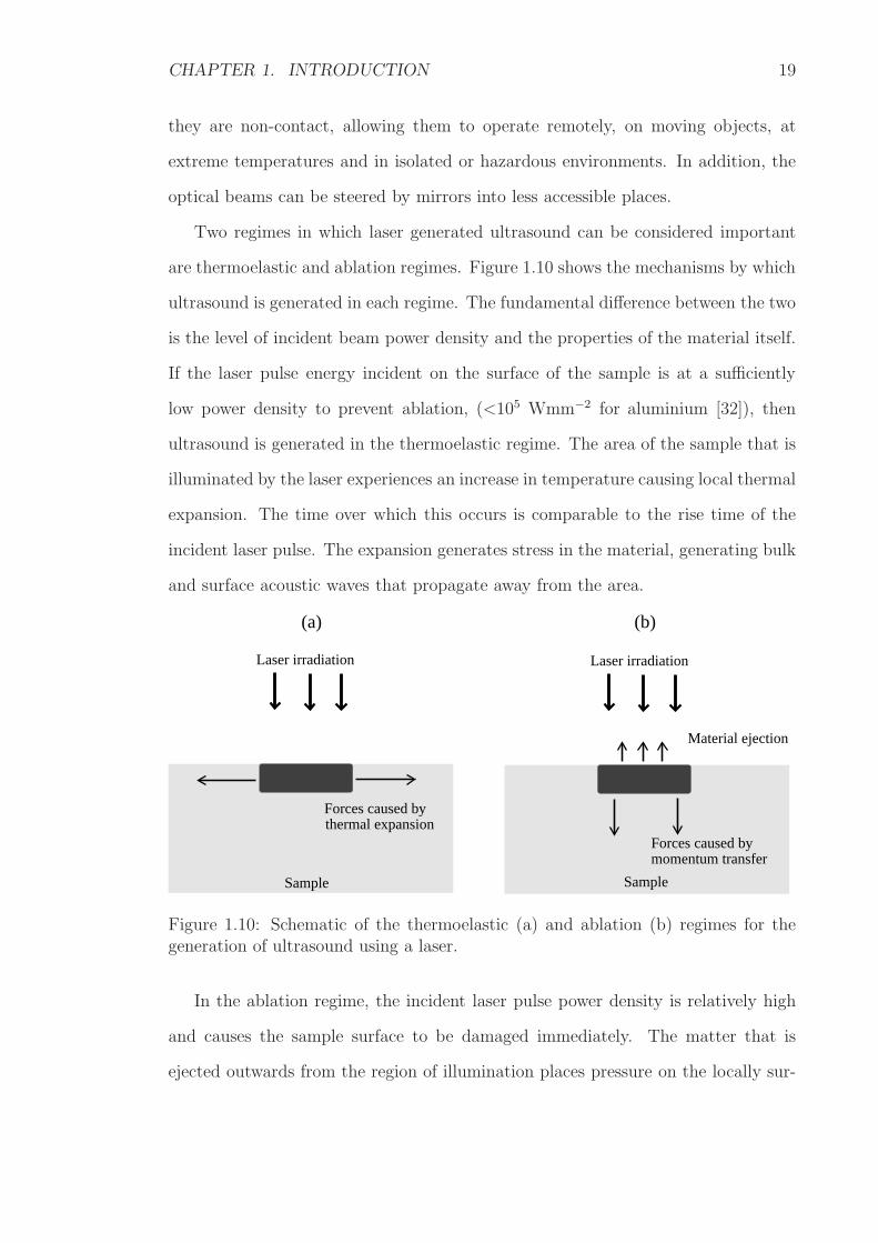
Two regimes in which laser generated ultrasound can be considered important
are thermoelastic and ablation regimes. Figure 1.10 shows the mechanisms by which
ultrasound is generated in each regime. The fundamental difference between the two
is the level of incident beam power density and the properties of the material itself.
If the laser pulse energy incident on the surface of the sample is at a sufficiently
low power density to prevent ablation, (<105 Wmm−2 for aluminium [32]), then
ultrasound is generated in the thermoelastic regime. The area of the sample that is
illuminated by the laser experiences an increase in temperature causing local thermal
expansion. The time over which this occurs is comparable to the rise time of the
incident laser pulse. The expansion generates stress in the material, generating bulk
and surface acoustic waves that propagate away from the area.
Forces caused bythermal expansion
Forces caused bymomentum transfer
Laser irradiation
Material ejection
SampleSample
(b)(a)
Laser irradiation
Figure 1.10: Schematic of the thermoelastic (a) and ablation (b) regimes for thegeneration of ultrasound using a laser.
In the ablation regime, the incident laser pulse power density is relatively high
and causes the sample surface to be damaged immediately. The matter that is
ejected outwards from the region of illumination places pressure on the locally sur-

CHAPTER 1. INTRODUCTION 20
rounding material, exerting stresses and generating both bulk and surface waves in
the material.
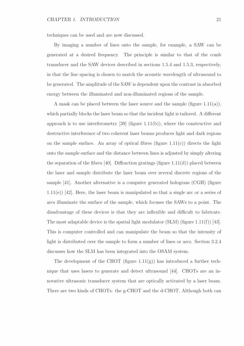
1.6.1 Review of laser generation techniques
Generating ultrasound using lasers can be achieved using several techniques that
differ in complexity (figure 1.11).
(g)
Incident laser light g−CHOT structure
S
L
MaskS
Lens
(c)
(a)
Multiple fibresS
L
S
L
beam profileSLM controls
BS
Diffraction grating
S
L
(b)
L
M
MBS
S
LensInterference
pattern
(e)
CGHS
L
(f)
(d)
Figure 1.11: Laser generation of ultrasound with a mask (a), interferometry (b),multiple fibres (c), diffraction grating (d), computer generated hologram (e), SLM(f), and g-CHOT (g). L=laser source, S=sample, BS=beamsplitter, M=mirror.
The less complex methods involve focusing the laser beam to a point [37] or a
line [38] and often this results in sample damage. To prevent damage, a number of
CHAPTER 1. INTRODUCTION 21
techniques can be used and are now discussed.
By imaging a number of lines onto the sample, for example, a SAW can be
generated at a desired frequency. The principle is similar to that of the comb
transducer and the SAW devices described in sections 1.5.4 and 1.5.3, respectively,
in that the line spacing is chosen to match the acoustic wavelength of ultrasound to
be generated. The amplitude of the SAW is dependent upon the contrast in absorbed
energy between the illuminated and non-illuminated regions of the sample.
A mask can be placed between the laser source and the sample (figure 1.11(a)),
which partially blocks the laser beam so that the incident light is tailored. A different
approach is to use interferometry [39] (figure 1.11(b)), where the constructive and
destructive interference of two coherent laser beams produces light and dark regions
on the sample surface. An array of optical fibres (figure 1.11(c)) directs the light
onto the sample surface and the distance between lines is adjusted by simply altering
the separation of the fibres [40]. Diffraction gratings (figure 1.11(d)) placed between
the laser and sample distribute the laser beam over several discrete regions of the
sample [41]. Another alternative is a computer generated hologram (CGH) (figure
1.11(e)) [42]. Here, the laser beam is manipulated so that a single arc or a series of
arcs illuminate the surface of the sample, which focuses the SAWs to a point. The
disadvantage of these devices is that they are inflexible and difficult to fabricate.
The most adaptable device is the spatial light modulator (SLM) (figure 1.11(f)) [43].
This is computer controlled and can manipulate the beam so that the intensity of
light is distributed over the sample to form a number of lines or arcs. Section 3.2.4
discusses how the SLM has been integrated into the OSAM system.
The development of the CHOT (figure 1.11(g)) has introduced a further tech-
nique that uses lasers to generate and detect ultrasound [44]. CHOTs are an in-
novative ultrasonic transducer system that are optically activated by a laser beam.
There are two kinds of CHOTs: the g-CHOT and the d-CHOT. Although both can

CHAPTER 1. INTRODUCTION 22
work independently of each other, a coupled CHOT system provides a powerful,
robust, sensitive and remotely operated technique.
1.6.2 The g-CHOT
The g-CHOT is a structure deposited onto the sample surface. The geometrical
characteristics of the structure control the generated wave mode, direction and
wavelength. The principle behind the making of the g-CHOT was to create an
ultrasonic source with an appropriately high contrast between absorbing and non-
absorbing regions of the irradiated sample. An example of a g-CHOT structure for
the generation of SAWs is shown in figure 1.12.
λ SAW
Sample
h
(a)
Elastic wave
Incident laser
y
z
x
(b) x
(c)
Amp
Amp
x
Figure 1.12: Basic g-CHOT cross section showing the structure required for SAWgeneration (a). Incident laser light illuminates a series of titanium lines separatedby one acoustic wavelength λSAW . g-CHOT profiles can be fabricated as a series oflines (b) and arcs (c) that generate plane and focused ultrasound.
The profile of the CHOT lines can be altered to control the direction of the
wave propagation. For example, by having a pattern with straight parallel lines, the
resulting SAWs will have a plane wavefront that would propagate from both ends of
the CHOT. The advantage of using an arc profile is that the ultrasound is focused
to a single point, improving the signal-to-noise-ratio (SNR) for point detection. In
this way the g-CHOT controls the directivity of the generated waves.
The incident radiation has to be pulsed since, otherwise a static thermal equilib-
rium would be reached between the absorbing and non-absorbing regions of the sam-

CHAPTER 1. INTRODUCTION 23
ple and in this condition, a SAW would not be excited. The pulsed laser light could
be considered to be analogous to the alternating current that was applied across the
two electrodes of a SAW device as described in section 1.5.3. The advantage of us-
ing light as the actuator, as opposed to an alternating current (AC) voltage, is that
no physical connection exists between transducer and actuator. Therefore, using a
laser offers a completely remotely operated and non-contact system for generating
ultrasound.
1.7 Detecting ultrasound with lasers
There are several laser detection techniques which can be broadly classified as either
interferometric and non-interferometric methods [45, 46, 39]. A disadvantage of
optical detection techniques compared with contacting transducers is that they are
relatively insensitive [47]. Another disadvantage of laser detection is that if the
sample surface is rough, the reflected beam is scattered. Possible solution to this
problem include the use of a Fabry-Perot interferometer [45, 48, 49], or a photo-emf
detector [50]. This section describes the knife-edge and interferometry techniques
used to detect ultrasound.
1.7.1 Knife-edge detection
The knife-edge detector, also referred to as the optical beam deflection technique,
[51, 52] can have several configurations (figure 1.13) [51].
The incident laser beam is focused onto the surface of the sample by a lens,
and the reflected beam is focused onto a single photodetector. In this case, a knife-
edge is placed over half of the reflected beam and a single photodiode converts the
detected light into a voltage signal. A propagating SAW causes the surface gradient
to change, which will deflect the reflected beam to a different position and alter the

CHAPTER 1. INTRODUCTION 24
Photodiode
Sample
knife−edge
Focusing lens Collecting lens
Figure 1.13: The knife edge detector. A propagating SAW causes the reflectedbeam to be shifted causing the light intensity, measured by the photodiode, to bemodulated.
intensity of light being focused onto the detector. The surface of the sample needs
to have a polished finish so that light scatter is minimised, and light incident on the
photodiode is maximised.
For the work in this thesis, an alternative knife-edge detector arrangement was
used (see section 3.3). Here, a differential detection technique is employed in which
the knife-edge is replaced by a second photodiode. The advantage with the differ-
ential method is that the common-mode noise (due to intensity fluctuations of the
probe beam) is reduced.
1.7.2 Interferometry
A common interferometer configuration is the Michelson interferometer [53, 54],
which is shown in figure 1.14.
The light emitted from the laser is divided into two beams. One of these beams
is incident on a reference mirror, which is held in a fixed position. The other beam is
incident on the surface of the sample. Both beams are reflected off their respective
elements and recombine at the beamsplitter, where they interfere either construc-
tively or destructively. The recombined beam is incident onto a detector, which
measures the intensity of the beam. Any change in path length brought on by the
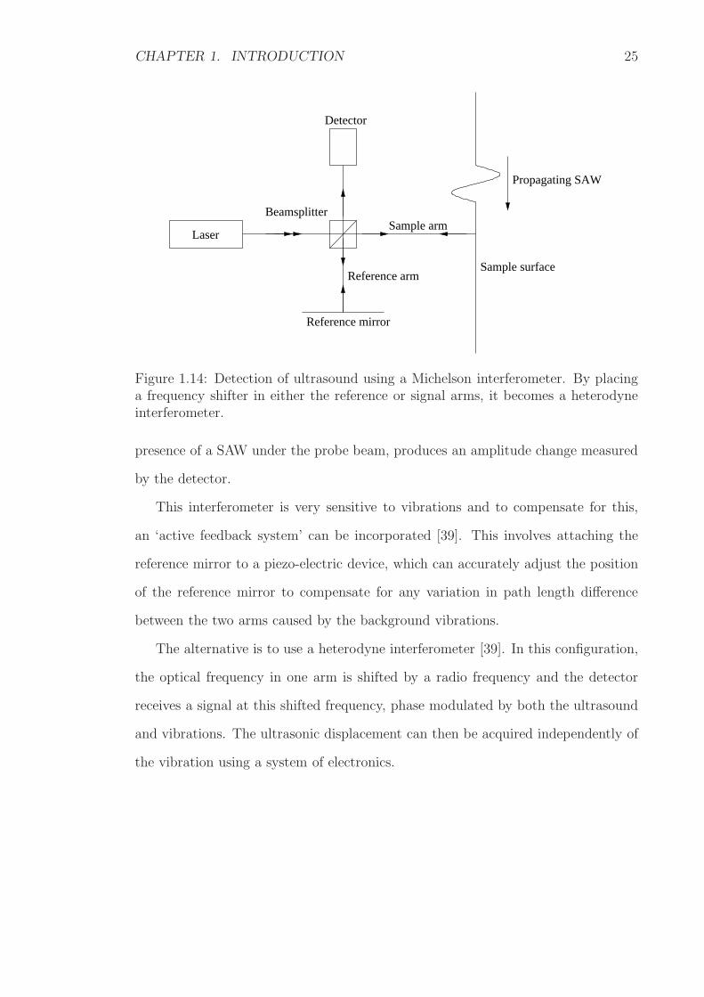
CHAPTER 1. INTRODUCTION 25
Detector
Reference mirror
Laser
Reference arm
Sample arm
Sample surface
Propagating SAW
Beamsplitter
Figure 1.14: Detection of ultrasound using a Michelson interferometer. By placinga frequency shifter in either the reference or signal arms, it becomes a heterodyneinterferometer.
presence of a SAW under the probe beam, produces an amplitude change measured
by the detector.
This interferometer is very sensitive to vibrations and to compensate for this,
an ‘active feedback system’ can be incorporated [39]. This involves attaching the
reference mirror to a piezo-electric device, which can accurately adjust the position
of the reference mirror to compensate for any variation in path length difference
between the two arms caused by the background vibrations.
The alternative is to use a heterodyne interferometer [39]. In this configuration,
the optical frequency in one arm is shifted by a radio frequency and the detector
receives a signal at this shifted frequency, phase modulated by both the ultrasound
and vibrations. The ultrasonic displacement can then be acquired independently of
the vibration using a system of electronics.

CHAPTER 1. INTRODUCTION 26
1.7.3 The d-CHOT
Since the g-CHOT (section 1.6.2) generates narrowband ultrasound, it is favourable
to have a matching narrowband detection system as well and this has led to the de-
velopment of the d-CHOT. As with the g-CHOT, the d-CHOT consists of a structure
placed onto the sample surface. However, as it reflects light, the d-CHOT can be
considered a reflective grating. It is designed so that its geometrical features will se-
lect the desired mode and frequency. The basic d-CHOT structure for the detection
of SAWs is shown in figure 1.15.
λElastic wave
h
ReflectedIncident
Laser source Detector
θ
Sample
Figure 1.15: Cross-section of basic d-CHOT structure with appropriate height (h)and spacing (λ) to detect SAWs. As with the g-CHOT, the lines can be set for thedetection of plane or focused waves.
The d-CHOT is activated by an incident continuous (CW) laser and the reflected
beam is separated into a number of diffraction orders. The line spacing is chosen
to ‘select’ or ‘match’ the acoustic wavelength of the waves that are to be detected.
The height of the steps in the grating is designed in such a way as to introduce the
desired path length difference in the incident light. The height of the steps is given
by equation 1.21.
h =λopt
8 cos(θ)(1.21)
where h is the step height, λopt is the optical wavelength of the incident laser and θ
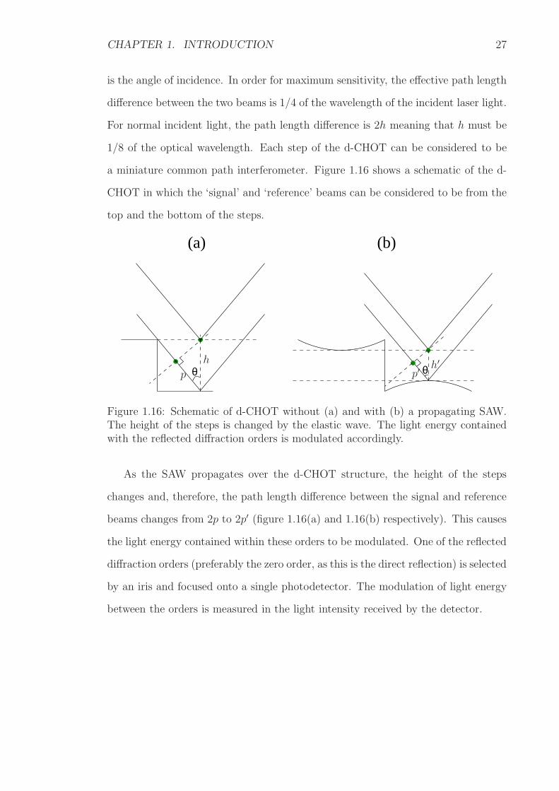
CHAPTER 1. INTRODUCTION 27
is the angle of incidence. In order for maximum sensitivity, the effective path length
difference between the two beams is 1/4 of the wavelength of the incident laser light.
For normal incident light, the path length difference is 2h meaning that h must be
1/8 of the optical wavelength. Each step of the d-CHOT can be considered to be
a miniature common path interferometer. Figure 1.16 shows a schematic of the d-
CHOT in which the ‘signal’ and ‘reference’ beams can be considered to be from the
top and the bottom of the steps.
θ θ
(a) (b)
h
ph′
p′
Figure 1.16: Schematic of d-CHOT without (a) and with (b) a propagating SAW.The height of the steps is changed by the elastic wave. The light energy containedwith the reflected diffraction orders is modulated accordingly.
As the SAW propagates over the d-CHOT structure, the height of the steps
changes and, therefore, the path length difference between the signal and reference
beams changes from 2p to 2p′ (figure 1.16(a) and 1.16(b) respectively). This causes
the light energy contained within these orders to be modulated. One of the reflected
diffraction orders (preferably the zero order, as this is the direct reflection) is selected
by an iris and focused onto a single photodetector. The modulation of light energy
between the orders is measured in the light intensity received by the detector.

CHAPTER 1. INTRODUCTION 28
1.8 Summary
The motivation behind this work is to develop a NDT method that can be applied
to monitoring material fatigue. To achieve this, the first objective is to establish
an experimental technique capable of measuring material nonlinearity. The second
objective is to apply the technique to fatigued samples. The level of fatigue would
cause the measured nonlinearity to change.
This thesis presents a laser-based ultrasonic experimental technique which aims
to fulfil the first of these objectives. The experiment measures a change in ultrasonic
velocity caused by an applied stress. The velocity-stress gradient is a direct measure
of material nonlinearity and can, therefore, be used to monitor fatigue.
The work presented here is novel because the experiment was performed using
SAWs which were generated and detected using lasers and therefore has the advan-
tage of being non-contacting.
Chapter 2
Literature Review
2.1 Introduction
The purpose of this chapter is to provide a review of material elastic behaviour
(section 2.2) and the nonlinear experimental techniques that are currently being
used in NDT (section 2.3). A broad historical overview of nonlinear ultrasound can
be found in [55] and [56].
Material nonlinearity manifests itself as acoustic-waveform distortion due to
amplitude-dependent wave propagation, higher harmonics generation, velocity mod-
ulation and the inter-modulation of two independent propagating waves (sum and
difference frequencies). Material nonlinearity is often quantified by the β-parameter,
defined in section 2.3.1. The work in this thesis does not use β, instead the velocity-
stress relationship is used to quantify material nonlinearity.
Fatigue is defined as the decline in mechanical properties encountered in a metal
subjected to repeated cycles of stress [57]. Fatigue damage is a distributed phe-
nomenon affecting the structure at many locations. Before the initiation of a termi-
nal crack, small-scale micro-cracking occurs, which can be considered to be an even
degradation of the material. These micro-cracks can be regarded as nuclei of the
fracture process and since the nuclei are much smaller than the acoustic wavelength
29
CHAPTER 2. LITERATURE REVIEW 30
at the frequencies generally used for NDT, linear acoustic indications (e.g. changes
in attenuation and velocity) have insufficient sensitivity to detect their presence.
However, micro-cracks do give rise to excess material nonlinearity, which can be or-
ders of magnitude higher than the intrinsic nonlinearity of an undamaged material.
A nonlinear ultrasonic technique locates fatigue by causing micro-cracks to open
and close (referred to as ‘clapping’). When a crack is forced to close, the local
elastic modulus approaches that of a continuous (undamaged) material. As a crack
is opened, the elastic modulus decreases. This parametric modulation in elastic
modulus is caused by the stress dependence of the interfacial stiffness of the crack.
In a fatigued material, the presence of local residual stresses cause cracks to be
partially open and these contribute to the excess nonlinearity [58, 59, 60]. Material
nonlinearity can be quantified by the β-parameter or by the velocity-stress gradient.
The presence of fatigue, would therefore cause these parameters to change.
The nonlinear methods discussed in this chapter are subjects of research in the
AERONEWS (health monitoring of aircraft by nonlinear elastic wave spectroscopy)
project and Delsanto (2007) [61] provides a complete and recent publication on the
application of these nonlinear experiments to non-destructive evaluation.
2.2 Linear elasticity
A material is said to be ‘linear’ if the relationship between stress and strain in the
elastic region of the material is constant, i.e. a constant Young’s modulus. In a
homogeneous, isotropic and linear material, the relationship between stress (σij)
and strain (ǫkl) is given by Hooke’s law, which states that the degree of strain is
linearly related to the applied stress (equation 2.1):
σij = Cijklǫkl (2.1)
CHAPTER 2. LITERATURE REVIEW 31
where Cijkl is the second order elastic constants (or the 4th rank stiffness tensor),
which has 81 components. Using a compressed (Voight) notation, the number of
components can be reduced to 36 and these components can be shown in a 6×6
matrix (equation 2.2).
σxx
σyy
σzz
σyz
σzx
σxy
=
C11 C12 C13 C14 C15 C16
C21 C22 C23 C24 C25 C26
C31 C32 C33 C34 C35 C36
C41 C42 C43 C44 C45 C46
C51 C52 C53 C54 C55 C56
C61 C62 C63 C64 C65 C66
ǫxx
ǫyy
ǫzz
ǫyz
ǫzx
ǫxy
(2.2)
For an isotropic solid the stiffness tensor matrix can be simplified since Cxy = Cyx
(reducing the number of constants to 21). Also, the following relations are true:
C11 = C22 = C33 = λ+ 2µ (2.3)
C44 = C55 = C66 = µ (2.4)
C12 = C13 = C21 = C23 = C31 = C32 = λ (2.5)
where λ and µ are the Lame constants (all other constants in the matrix are zero).
The Lame constants are known as the second order elastic constants, and together
they can be used to completely describe the elastic behaviour of an isotropic solid.
They are related to the Young’s modulus (E), Poisson’s ratio (ν) and bulk modulus
(K) by equations 2.6, 2.7 and 2.8, respectively.
E =µ(3λ+ 2µ)
λ+ µ(2.6)

CHAPTER 2. LITERATURE REVIEW 32
ν =λ
2(λ+ µ)(2.7)
K = λ+2
3µ (2.8)
In a solid, the relationship between sound velocity, v and the elastic constants is
given by equation 2.9 [62].
v =
√
Cxy
ρ(2.9)
where ρ is the material density. The shear velocity (vs) and longitudinal velocity (vl)
are calculated by substituting Cxy with the shear (G) or longitudinal (L) moduli,
respectively. G and L are given in equations 2.10 and 2.11, respectively [63]:
G =E
2(1 + ν)(2.10)
L = K +4
3G (2.11)
A Rayleigh wave has both shear and longitudinal contributions, and the Rayleigh
wave velocity (vr) can be obtained using the Bergmann approximation [3]:
vr
vs
=0.87 + 1.12ν
1 + ν(2.12)
In the linear regime, the elastic constants (and, therefore, the ultrasonic velocity)
are unaltered by applied stress, providing that all other variables such as temperature
[64], remain constant. However, there have been numerous experiments that have
disproved this. For example, when steel and silicon nitride samples were placed into a
4-point bending jig, it was found that the velocity of SAWs changed with stress [13].
For steel, the Rayleigh wave velocity was found to change by −5.76mms−1/MPa

CHAPTER 2. LITERATURE REVIEW 33
and for silicon nitride, a velocity change of approximately 52.6mms−1/MPa was
measured.
2.3 Nonlinear experimental techniques
There are numerous experimental techniques that are being used to measure material
nonlinearity. The purpose of this section is to review these methods and discuss their
advantages and disadvantages.
2.3.1 Higher harmonic generation − ‘self-stressing’ method
In a ‘nonlinear material’, a high amplitude wave experiences an accumulative in-
crease in distortion (in addition to attenuation and diffraction) as it propagates
[65]. The reason for this is because different parts of the wave propagate at different
velocities. This type of wave can be considered as ‘self-stressing’, i.e. the velocity of
the wave depends on the stress that it is imposing on the sample (figure 2.1 [65]).
V0 V0
V−
V+
V0
Direction of propagation
Nonlinear sample
Figure 2.1: Propagation of a high amplitude (‘self-stressing’) wave in an elasticmaterial. As the propagation distance increases, the wave profile becomes distorted.The harmonic content of the wave can be obtained to provide a measure of thematerial nonlinearity.
In figure 2.1 the peak and trough of the wave are propagating faster and slower

CHAPTER 2. LITERATURE REVIEW 34
respectively than the zero stress position, causing the wave to become distorted.
The degree of distortion depends on the material type, the wave amplitude and
how far the wave has propagated. In the case of an undamaged elastic material,
this is a gradual effect. Contrastingly, in the presence of internal stresses, micro-
fatigue cracks and damage, it can occur suddenly, since these significantly increase
the nonlinear response of the material.
The wave distortion causes the frequency content of the wave to change because
the acoustic energy is transferred from the fundamental frequency to its harmonics.
This is different from the pump-probe method used in this thesis, in which the
‘stressing’ and ‘velocity measuring’ were performed by two independent waves.
By measuring the harmonic(s) amplitude relative to the fundamental, it is pos-
sible to obtain a measure of material nonlinearity. Equation 2.13 relates the ratio
of the fundamental and second harmonic with this nonlinearity, in terms of the
β-parameter.
β = (A2
A21
)8
kd(2.13)
where A1 and A2 are the amplitudes of the fundamental and second harmonic com-
ponents of the detected ultrasound, respectively, k is the propagation constant (2πλ
)
and d is the distance over which the wave has propagated. The experimental prin-
ciple is, therefore, to excite a wave in the sample at frequency f and detect at
frequencies f and 2f. This is a very popular technique [66, 67, 68, 69, 70, 71, 72],
and has been used to investigate the effect of dislocation density [73] using various
detection techniques such as a capacitive transducer [74], optical probing [75] and
Michelson interferometry [76, 77]. Recently, the harmonic generation technique has
been performed with a Rayleigh wave [78].
The experiment performed by Blackshire et al aimed to detect the presence of a
fracture in titanium samples [79]. A 5MHz bulk wave was generated and as the sound
CHAPTER 2. LITERATURE REVIEW 35
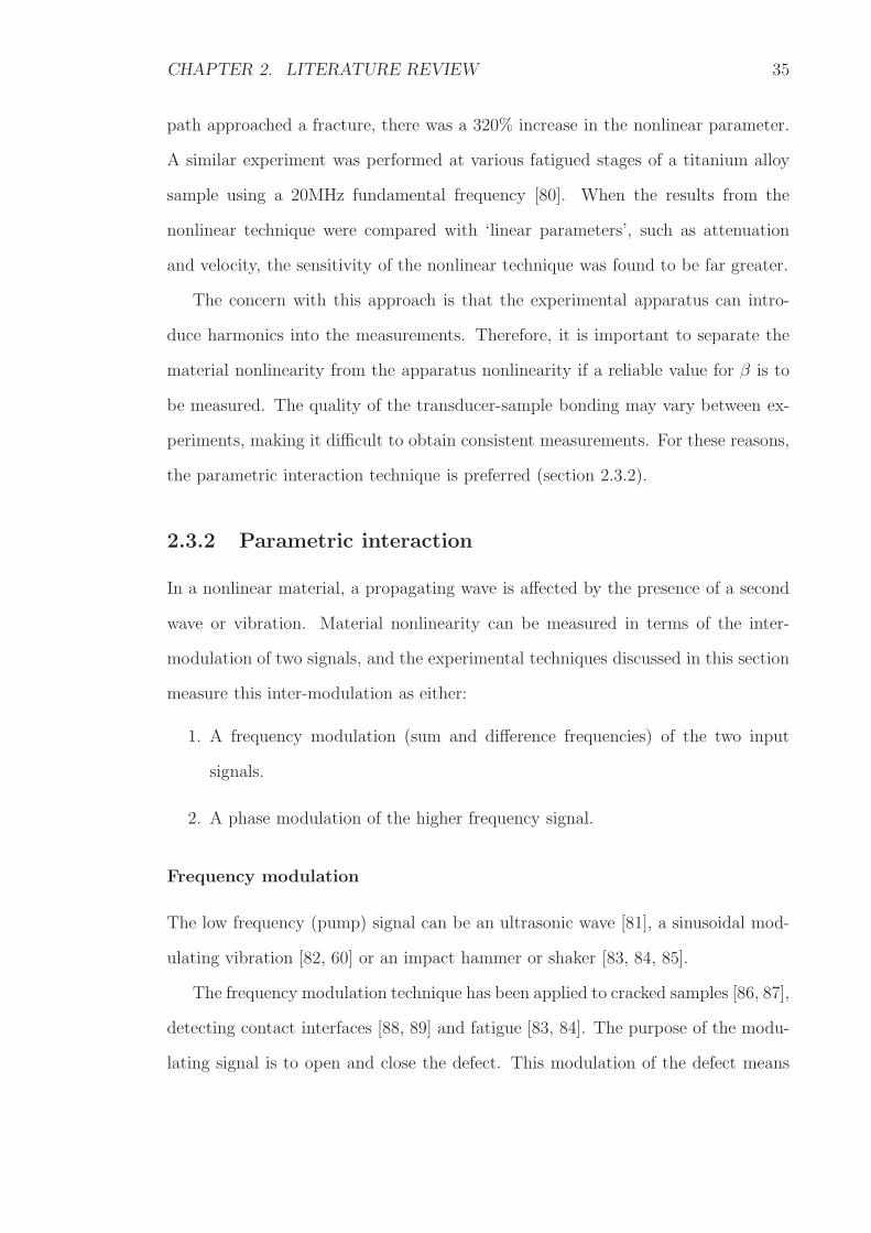
path approached a fracture, there was a 320% increase in the nonlinear parameter.
A similar experiment was performed at various fatigued stages of a titanium alloy
sample using a 20MHz fundamental frequency [80]. When the results from the
nonlinear technique were compared with ‘linear parameters’, such as attenuation
and velocity, the sensitivity of the nonlinear technique was found to be far greater.
The concern with this approach is that the experimental apparatus can intro-
duce harmonics into the measurements. Therefore, it is important to separate the
material nonlinearity from the apparatus nonlinearity if a reliable value for β is to
be measured. The quality of the transducer-sample bonding may vary between ex-
periments, making it difficult to obtain consistent measurements. For these reasons,
the parametric interaction technique is preferred (section 2.3.2).
2.3.2 Parametric interaction
In a nonlinear material, a propagating wave is affected by the presence of a second
wave or vibration. Material nonlinearity can be measured in terms of the inter-
modulation of two signals, and the experimental techniques discussed in this section
measure this inter-modulation as either:
1. A frequency modulation (sum and difference frequencies) of the two input
signals.
2. A phase modulation of the higher frequency signal.
Frequency modulation
The low frequency (pump) signal can be an ultrasonic wave [81], a sinusoidal mod-
ulating vibration [82, 60] or an impact hammer or shaker [83, 84, 85].
The frequency modulation technique has been applied to cracked samples [86, 87],
detecting contact interfaces [88, 89] and fatigue [83, 84]. The purpose of the modu-
lating signal is to open and close the defect. This modulation of the defect means
CHAPTER 2. LITERATURE REVIEW 36
that the high frequency (probe) signal (generated by a transducer, for example) will
become distorted as it propagates through the defect. The combined result of the
pump and (distorted) probe waves generates side bands in the frequency spectrum.
The modulation of the defect can be achieved using an incident laser source, which
thermally expands and contracts the material around the crack [90].
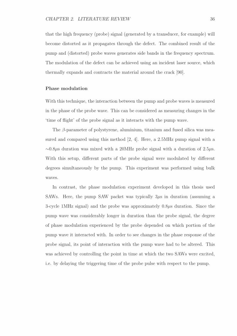
Phase modulation
With this technique, the interaction between the pump and probe waves is measured
in the phase of the probe wave. This can be considered as measuring changes in the
‘time of flight’ of the probe signal as it interacts with the pump wave.
The β-parameter of polystyrene, aluminium, titanium and fused silica was mea-
sured and compared using this method [2, 4]. Here, a 2.5MHz pump signal with a
∼0.8µs duration was mixed with a 20MHz probe signal with a duration of 2.5µs.
With this setup, different parts of the probe signal were modulated by different
degrees simultaneously by the pump. This experiment was performed using bulk
waves.
In contrast, the phase modulation experiment developed in this thesis used
SAWs. Here, the pump SAW packet was typically 3µs in duration (assuming a
3-cycle 1MHz signal) and the probe was approximately 0.8µs duration. Since the
pump wave was considerably longer in duration than the probe signal, the degree
of phase modulation experienced by the probe depended on which portion of the
pump wave it interacted with. In order to see changes in the phase response of the
probe signal, its point of interaction with the pump wave had to be altered. This
was achieved by controlling the point in time at which the two SAWs were excited,
i.e. by delaying the triggering time of the probe pulse with respect to the pump.
CHAPTER 2. LITERATURE REVIEW 37
2.3.3 Nonlinear-time reversal acoustics (NL-TRA)
The time reversal (TR) technique can be applied to the harmonic generation and
wave modulation techniques described above [91]. To describe how TR is imple-
mented, this section will focus on its application to the harmonic generation tech-
nique.
A single emitting transducer generates ultrasound into the sample. This ultra-
sound is then detected at various locations around the sample using a number of
detecting transducers and the signals that these detector transducers obtain are then
time reversed. The detector transducers are then converted to emitters and what
was the emitter transducer is now converted to a detector. The emitter transduc-
ers now generate their respective TR signals, which recombine with each other as
they propagate back through the material. If the material is completely linear and
damage-free, then there will be no harmonic content in any of the signals. Therefore,
this recombined signal, which is the superposition of all these TR signals, will be
detected by the detection transducer. However, if the sample is damaged and, there-
fore, has a higher nonlinearity content, then harmonics will have been generated.
On sending back the TR signals in a damaged material, the harmonic contributions
would recombine at the focus of their source, i.e. at the damaged region. Mean-
while, the fundamental components of the TR signals would recombine back at their
source, i.e. at the detector transducer. A highpass filter could be applied to the
TR signals ensuring that only the harmonic contributions would be sent back into
the sample. By imaging the ultrasound on the sample surface with a laser detection
system, for example, the area of damage can be located.
2.3.4 Nonlinear reverberation spectroscopy (NRS)
The aim of NRS is to identify the presence of damage in a component, rather than
specifically locating the precise area of damage [92]. A sample is globally excited

CHAPTER 2. LITERATURE REVIEW 38
by a mono-frequency source at a constant amplitude for a known duration of time.
A loud speaker, placed relatively near the sample, is used to generate a frequency
close to the resonant frequency of the specimen. The duration over which this
frequency is emitted has to be long enough for the sample to reach a steady state
response. The transmitting sound is then stopped and the reverberation response
from the specimen is recorded. This detection is carried out either with a laser
vibrometer or with a contact transducer which is sensitive to this resonant frequency.
The detected signal, consisting of a decaying time signal, is then analysed. This
waveform is broken up into several time windows, each with typically a 20-cycle
duration. Exponentially decaying sine functions are then fitted to each window
and the frequency content between each window is compared. If the material is
linear and damage-free, then there is no change in frequency content between the
windowed data. However, the presence of damage means that the reverberation
signal frequency content increases with time. This can then be plotted directly as a
function of amplitude of the reverberation signal.
Materials such as carbon fibre reinforced plastics (CFRP) have produced positive
nonlinear measurements [92]. Here, a number of samples were exposed to different
temperatures to change the elastic (i.e. nonlinear) properties of the material.
The NRS technique is useful to globally test for damage in a given sample or
component and, therefore, would lend itself well to a ‘pass or fail’ test scenario,
but to actually locate the precise region of damage, further experimental techniques
would also incorporated.
2.4 Summary
This chapter began with a review of material elasticity and showed how stress and
ultrasonic velocity are related. Numerous nonlinear experimental methods were
described including the higher harmonic generation method, parametric interaction,
CHAPTER 2. LITERATURE REVIEW 39
NL-TRA and NRS. Most of these techniques are sensitive to material nonlinearity
brought on by the presence of a crack or a region of damaged material. The ability
to identify the location, or even simply detect the presence of damage within a
specimen minimises the risk of failure while in use. However, NDT techniques
capable of measuring changes in material nonlinearity before the initiation of a
crack are a very important tool that would have applications in a broad range of
industries. This would require an extremely sensitive experimental technique, but if
it was possible, it would allow the identification of potentially problematic specimen
areas thereby minimising the risk of catastrophic failure of a component.
Using this knowledge obtained from these nonlinear techniques, accurate toler-
ances for various parts of an aircraft could be specified. The experimental method
presented in this thesis is capable of measuring material nonlinearity and the next
stage in the development of this method would be to apply it to fatigued samples.
At the very early stages of fatigue, nonlinear measurements are efficient at de-
tecting damage. However, if too many microcracks appear (or if the microcracks
become too large) in the area on the sample, then it becomes difficult for the ultra-
sound to propagate through the material. In this case, a linear ultrasonic technique
(e.g. wave reflection) could be considered a more suitable approach.

Chapter 3
Instrumentation
3.1 Introduction
This chapter will describe the OSAM instrument, in terms of its optical and elec-
tronic configuration, the generation and detection setups, and the calibration pro-
cedure for the knife-edge detector. Finally the high speed analogue electronics used
to acquire the magnitude and phase information of the detected ultrasound will be
described. This set of electronics was not used for the nonlinear experiment, however
it proved useful for taking aerial point spread functions (PSFs) of several samples,
which have been included in section 1.6.2.
3.2 Optical setup for the generation of ultrasound
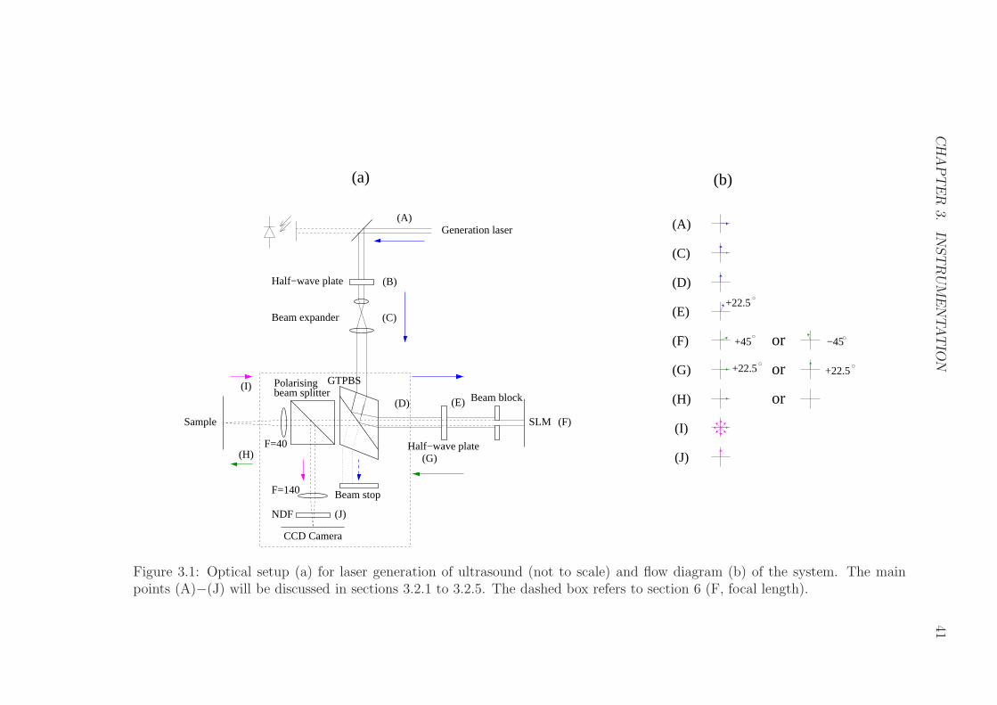
The optical system used for the generation of ultrasound is shown in figure 3.1.
40
CH
AP
TE
R3.
INST
RU
ME
NTA
TIO
N41
+22.5
(A)
(C)
(D)
(E)
(F)
(G)
(H)
(I)
(J)
+45
+22.5 +22.5
−45
(H)
(a)
beam splitter
(b)
Generation laser
Half−wave plate
Beam expander
SLM
Beam block
Half−wave plate
Sample
F=140
F=40
NDF
Beam stop
GTPBSPolarising
CCD Camera
or
or
or
(J)
(G)
(I)
(D) (E)
(B)
(C)
(A)
(F)
Figure 3.1: Optical setup (a) for laser generation of ultrasound (not to scale) and flow diagram (b) of the system. The mainpoints (A)−(J) will be discussed in sections 3.2.1 to 3.2.5. The dashed box refers to section 6 (F, focal length).
CHAPTER 3. INSTRUMENTATION 42
3.2.1 Generation source
The generation laser (A) is a Q-switched and mode-locked infra-red (IR) laser that
emits light at a wavelength of 1064nm. In order to generate SAWs, the laser has
to be pulsed and this is the purpose of the mode-locker. By pulsing the laser, the
sample surface that is illuminated by the beam experiences thermal expansion and
contraction at the same rate as the pulsing frequency. This dictates the frequency
of the generated SAW. A mode-locker is an acousto-optical device placed in the
laser cavity and its frequency of operation, f is related to the laser cavity length by
equation 3.1.
f =c
2L(3.1)
where c is the speed of light and L is the cavity length. The laser cavity is 1.83m
in length, meaning the fundamental frequency of the laser is 82MHz. In the mode-
locked state, the laser generates a continuous train of pulses, which are separated
by 1/82×106s. The duration of each pulse is 200ps and since these pulses are very
short in time, the laser output has a high harmonic content.
The Q-switcher can operate at repetition rates ranging from a few hundred hertz
up to 100kHz, although with higher frequencies, the peak power levels off and is
eventually reduced. In the OSAM system, the Q-switcher operates at 1015Hz, and
is dictated by the operating frequency of the SLM.
Between each trigger event of the Q-switcher, the energy within the laser accu-
mulates and is then released over a 0.4µs time window. In this way, the Q-switcher
increases the peak optical power of the laser source, thereby increasing the ampli-
tude of the generated SAW. The average optical power output from this laser system
has been measured at 2.4W. There are approximately 30 pulses in each Q-switched
burst, equating to 80µJ/pulse.

CHAPTER 3. INSTRUMENTATION 43
The horizontally-polarised light emitted from the generation laser is directed
onto a half-wave plate (B) using a mirror (reflectance >99.2%). The light that
is transmitted by the mirror is incident onto a photodetector, which provides a
‘coherent trigger pulse’. Figure 3.2(a) shows the output of the photodetector and
figure 3.2(b) is the Fourier transform of the signal.
0 0.1 0.2 0.3 0.4 0.5 0.6 0.7 0.8 0.9 1−0.2
0
0.2
0.4
0.6
0.8
1
1.2
Time (µs)
Am
plitu
de (
arb.
uni
ts)
0 100 200 300 400 500 600 700 8000
500
1000
1500
2000
Frequency (MHz)
Am
plitu
de (
arb.
uni
ts)
sµ( )Time
Am
plitu
de (
arb.
uni
ts)
Am
plitu
de (
arb.
uni
ts)
Frequency (MHz)
(a)
(b)
Figure 3.2: The coherent trigger pulse in the time (a) and frequency (b) domainsdetected by the photodiode placed at the end of the laser cavity.
In theory, the amplitude of all the harmonics should have the same amplitude

CHAPTER 3. INSTRUMENTATION 44
as the fundamental frequency up to 5GHz (since 200ps pulses), however, because
the photodetector (and electronics) has a limited bandwidth, the amplitude of the
harmonics decreases at higher frequencies (figure 3.2(b)).
3.2.2 Beam expansion
The Glan Taylor polarising beam splitter reflects vertically-polarised light towards
the SLM and transmits horizontally polarised light towards the beam stop. There-
fore, it is important to maximise the vertically-polarised contribution incident on
the beam splitter. This is achieved by placing a power meter after the beam splitter
and rotating the halfwave plate (B) until maximum light power is measured.
The active area of the SLM is 7.68×7.68mm and it is important to illuminate as
much of this as possible. The beam emitted directly from the laser has a diameter
of approximately 1.5mm, meaning that an expansion ratio of 5 is required. Between
the halfwave plate and the Glan Taylor beam splitter is a beam expander (C) that
uses a combination of two lenses (figure 3.3).
f1 f2
W2W1From laser To Glan Taylorpolarising beam splitter
Figure 3.3: Beam expander optical set-up.
The magnification factor is determined by the focal length ratio of the two lenses
and is related to the beam diameters before (W1) and after (W2) expansion by
equation 3.2.
W2
W1=f2
f1(3.2)
where f1 and f2 are the focal lengths of the lenses and are 40mm and 180mm,
respectively.
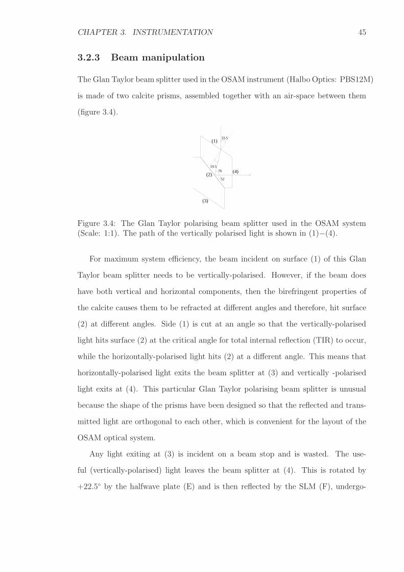
CHAPTER 3. INSTRUMENTATION 45
3.2.3 Beam manipulation
The Glan Taylor beam splitter used in the OSAM instrument (Halbo Optics: PBS12M)
is made of two calcite prisms, assembled together with an air-space between them
(figure 3.4).
33.5
19.576
52
(1)
(2)(4)
(3)
Figure 3.4: The Glan Taylor polarising beam splitter used in the OSAM system(Scale: 1:1). The path of the vertically polarised light is shown in (1)−(4).
For maximum system efficiency, the beam incident on surface (1) of this Glan
Taylor beam splitter needs to be vertically-polarised. However, if the beam does
have both vertical and horizontal components, then the birefringent properties of
the calcite causes them to be refracted at different angles and therefore, hit surface
(2) at different angles. Side (1) is cut at an angle so that the vertically-polarised
light hits surface (2) at the critical angle for total internal reflection (TIR) to occur,
while the horizontally-polarised light hits (2) at a different angle. This means that
horizontally-polarised light exits the beam splitter at (3) and vertically -polarised
light exits at (4). This particular Glan Taylor polarising beam splitter is unusual
because the shape of the prisms have been designed so that the reflected and trans-
mitted light are orthogonal to each other, which is convenient for the layout of the
OSAM optical system.
Any light exiting at (3) is incident on a beam stop and is wasted. The use-
ful (vertically-polarised) light leaves the beam splitter at (4). This is rotated by
+22.5 by the halfwave plate (E) and is then reflected by the SLM (F), undergo-
CHAPTER 3. INSTRUMENTATION 46
ing a +45 or −45 rotation accordingly (the reason for this is described in section
3.2.4). When passing back through the halfwave plate, the light experiences another
+22.5 rotation (G). At this point, the light is either horizontally or vertically po-
larised, depending on the SLM and will be either transmitted or reflected by the
Glan Taylor beam splitter respectively.
The horizontally polarised light passes back through the Glan Taylor beam split-
ter, through a second polarising beam splitter (the purpose of which will be described
in section 3.2.5) and is focused by a lens onto the surface of the sample (H). Mean-
while, the vertically polarised light is reflected by the Glan Taylor beam splitter
back towards the generation laser.
Between the halfwave plate and the SLM is an aperture comprising a rectangular
window. Its purpose is to absorb the laser beam energy that would otherwise fall
onto the highly sensitive electronics surrounding the active part of the SLM, thereby
removing the potential for damage.
3.2.4 SLM
The SLM is an analogue ferroelectric liquid crystal-spatial light modulator (FLC-
SLM) system developed by Boulder Nonlinear Systems Incorporated (BNS). The
purpose of the SLM is to manipulate the light that is reflected from it into a required
intensity profile or distribution, which is then focused onto the sample. It has a
512×512 pixel array with a 15µm pitch and an overall size of 7.68×7.68mm. The
approximate size of the SLM image on the sample surface is 2×2mm.
Each individual pixel can be regarded as a reflective halfwave plate and the
polarisation angle of the reflected light is controlled by an applied voltage that has
256 discrete states and is in turn, controlled by the host computer. Using these input
voltages, the angle of rotation ranges from −45 (control level 0) to +45 (control
level 255), relative to the incident polarisation angle.
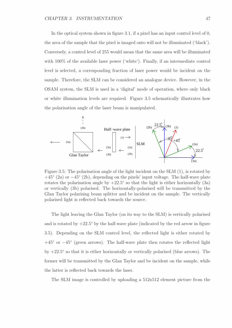
CHAPTER 3. INSTRUMENTATION 47
In the optical system shown in figure 3.1, if a pixel has an input control level of 0,
the area of the sample that the pixel is imaged onto will not be illuminated (‘black’).
Conversely, a control level of 255 would mean that the same area will be illuminated
with 100% of the available laser power (‘white’). Finally, if an intermediate control
level is selected, a corresponding fraction of laser power would be incident on the
sample. Therefore, the SLM can be considered an analogue device. However, in the
OSAM system, the SLM is used in a ‘digital’ mode of operation, where only black
or white illumination levels are required. Figure 3.5 schematically illustrates how
the polarisation angle of the laser beam is manipulated.
22.5o
−45o
+45o
22.5o
SLM
Half−wave plate
(3a)
(3b)
(1)
(2a)
(2b)
(3b)
Glan Taylor
(2b) (1)(3b)
(2a)
(3a)
(3a)
Figure 3.5: The polarisation angle of the light incident on the SLM (1), is rotated by+45 (2a) or −45 (2b), depending on the pixels’ input voltage. The half-wave platerotates the polarisation angle by +22.5 so that the light is either horizontally (3a)or vertically (3b) polarised. The horizontally-polarised will be transmitted by theGlan Taylor polarising beam splitter and be incident on the sample. The verticallypolarised light is reflected back towards the source.
The light leaving the Glan Taylor (on its way to the SLM) is vertically polarised
and is rotated by +22.5 by the half-wave plate (indicated by the red arrow in figure
3.5). Depending on the SLM control level, the reflected light is either rotated by
+45 or −45 (green arrows). The half-wave plate then rotates the reflected light
by +22.5 so that it is either horizontally or vertically polarised (blue arrows). The
former will be transmitted by the Glan Taylor and be incident on the sample, while
the latter is reflected back towards the laser.
The SLM image is controlled by uploading a 512x512 element picture from the
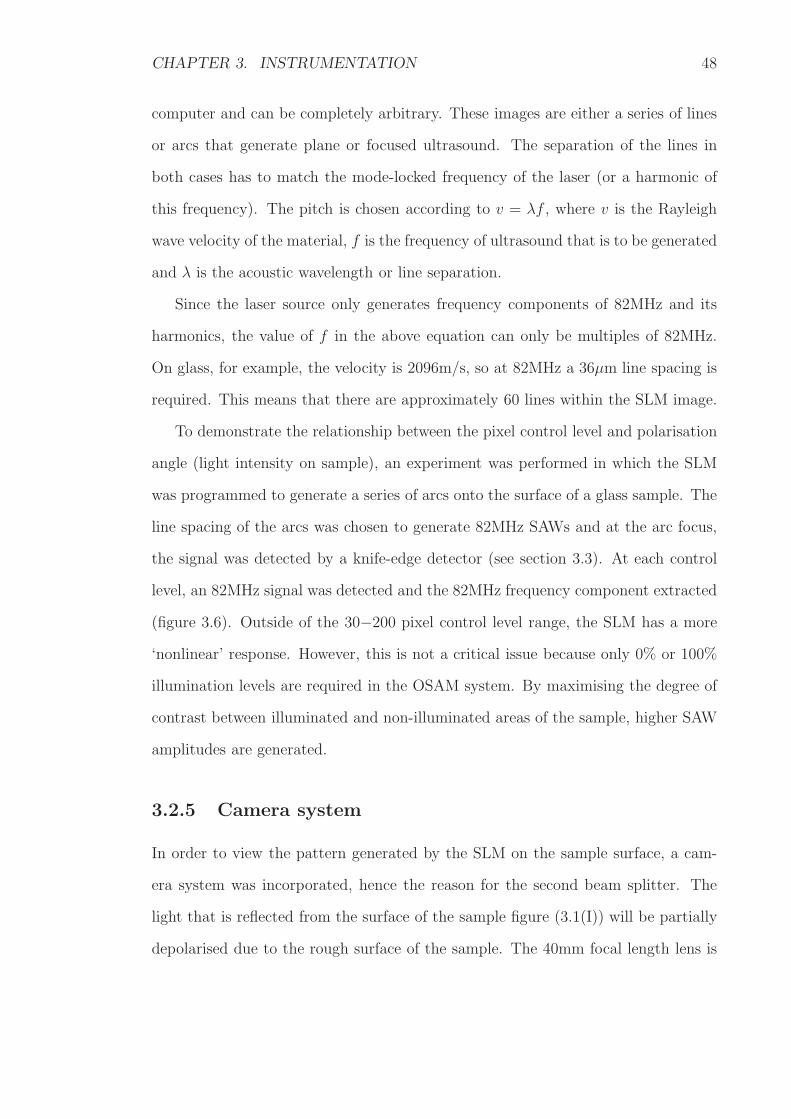
CHAPTER 3. INSTRUMENTATION 48
computer and can be completely arbitrary. These images are either a series of lines
or arcs that generate plane or focused ultrasound. The separation of the lines in
both cases has to match the mode-locked frequency of the laser (or a harmonic of
this frequency). The pitch is chosen according to v = λf , where v is the Rayleigh
wave velocity of the material, f is the frequency of ultrasound that is to be generated
and λ is the acoustic wavelength or line separation.
Since the laser source only generates frequency components of 82MHz and its
harmonics, the value of f in the above equation can only be multiples of 82MHz.
On glass, for example, the velocity is 2096m/s, so at 82MHz a 36µm line spacing is
required. This means that there are approximately 60 lines within the SLM image.
To demonstrate the relationship between the pixel control level and polarisation
angle (light intensity on sample), an experiment was performed in which the SLM
was programmed to generate a series of arcs onto the surface of a glass sample. The
line spacing of the arcs was chosen to generate 82MHz SAWs and at the arc focus,
the signal was detected by a knife-edge detector (see section 3.3). At each control
level, an 82MHz signal was detected and the 82MHz frequency component extracted
(figure 3.6). Outside of the 30−200 pixel control level range, the SLM has a more
‘nonlinear’ response. However, this is not a critical issue because only 0% or 100%
illumination levels are required in the OSAM system. By maximising the degree of
contrast between illuminated and non-illuminated areas of the sample, higher SAW
amplitudes are generated.
3.2.5 Camera system
In order to view the pattern generated by the SLM on the sample surface, a cam-
era system was incorporated, hence the reason for the second beam splitter. The
light that is reflected from the surface of the sample figure (3.1(I)) will be partially
depolarised due to the rough surface of the sample. The 40mm focal length lens is

CHAPTER 3. INSTRUMENTATION 49
0 50 100 150 200 2500
0.1
0.2
0.3
0.4
0.5
0.6
0.7
0.8
0.9
1
Level
82M
Hz
dete
cted
sig
nal (
arb.
uni
ts)
Figure 3.6: The detected 82MHz SAW with increasing pixel control level. At level256, maximum contrast is obtained.
used to collect this light, which is then directed by the second beam splitter to the
charge-coupled device (CCD) camera. A 140mm lens is used to focus the light onto
the camera. A neutral density filter (NDF) is placed in front of the CCD camera
(J) to reduce the light intensity on the camera and optimise the image.
3.3 Knife-edge detector
The detection system used in the OSAM instrument was a knife-edge detector. The
general principle has been reviewed in section 1.7.1, and the following sections will
explain how the detector is configured in terms of the optics and electronics.
3.3.1 Optical configuration
The OSAM instrument uses a knife-edge detector comprising two photodiodes (fig-
ure 3.7). The reflected beam from the sample surface oscillates between the two
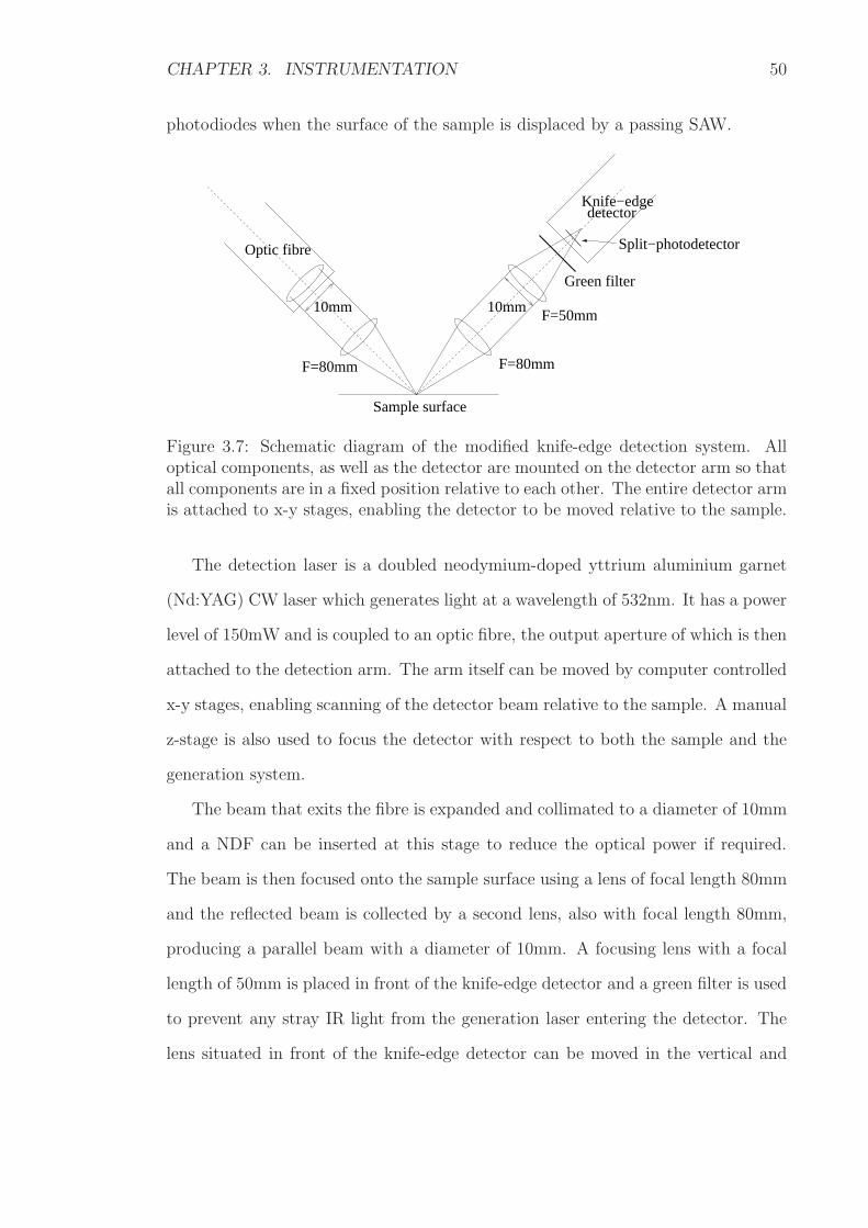
CHAPTER 3. INSTRUMENTATION 50
photodiodes when the surface of the sample is displaced by a passing SAW.
10mm
Knife−edgedetector
Optic fibre
Green filter
10mm
F=80mm
F=50mm
F=80mm
Split−photodetector
Sample surface
Figure 3.7: Schematic diagram of the modified knife-edge detection system. Alloptical components, as well as the detector are mounted on the detector arm so thatall components are in a fixed position relative to each other. The entire detector armis attached to x-y stages, enabling the detector to be moved relative to the sample.
The detection laser is a doubled neodymium-doped yttrium aluminium garnet
(Nd:YAG) CW laser which generates light at a wavelength of 532nm. It has a power
level of 150mW and is coupled to an optic fibre, the output aperture of which is then
attached to the detection arm. The arm itself can be moved by computer controlled
x-y stages, enabling scanning of the detector beam relative to the sample. A manual
z-stage is also used to focus the detector with respect to both the sample and the
generation system.
The beam that exits the fibre is expanded and collimated to a diameter of 10mm
and a NDF can be inserted at this stage to reduce the optical power if required.
The beam is then focused onto the sample surface using a lens of focal length 80mm
and the reflected beam is collected by a second lens, also with focal length 80mm,
producing a parallel beam with a diameter of 10mm. A focusing lens with a focal
length of 50mm is placed in front of the knife-edge detector and a green filter is used
to prevent any stray IR light from the generation laser entering the detector. The
lens situated in front of the knife-edge detector can be moved in the vertical and

CHAPTER 3. INSTRUMENTATION 51
horizontal planes to ensure that the beam is accurately focussed and covers equal
areas of the two detectors.
As the sample surface is tilted by a passing SAW, the reflected beam is shifted.
In order for the detector to sense the surface tilt, the photodiodes have to be placed
either slightly in front or behind the beam focus (i.e. a 180 phase difference exists
between the two positions).
3.3.2 Electronic configuration
The knife-edge detector consists of two sets of electronics, termed as the ‘front-end’
and ‘back-end’ electronics. Both will be described in this section, however, first it is
important to describe where these fit into the overall detector system (figure 3.8).
Knife−edgedetector
Filter
− +R
L
Analogueelectronics
A/Dcard
0
L−R L+R
Computer
RF signalAC path
Light
DC path
ZFL−500LN
Back−end electronics
Front−end electronics
Oscilloscope
Figure 3.8: Schematic of the complete detector system. The front-end and back-endelectronic sections of the knife-edge detector are outlined in bolded boxes. The ana-logue electronics (dashed box) were not permanently connected to the experimentalapparatus.
There are two output paths from the front-end electronics of the knife-edge de-
tector. The first is the alternating current (AC) path, in which the radio-frequency
(RF) signal (generated by the ultrasound) is amplified, filtered and observed on an
CHAPTER 3. INSTRUMENTATION 52
oscilloscope. The data required for the nonlinear experiment were obtained using
the oscilloscope. Occasionally, the analogue electronic system (that outputs the real
and imaginary components of the RF signal to the analogue-to-digital converter
[A/D] card in the computer) was used for acquiring c-scans and aerial PSFs. As the
analogue electronics were not used for the nonlinear experiment, it was not perma-
nently connected to the detection system and, therefore, is discussed separately in
section 3.5.
The second output path from the front-end electronics is the direct current (DC)
path, consisting of a ‘left’ and a ‘right’ channel corresponding to their respective
photodiodes. The information obtained from these channels was used to balance the
knife-edge detector so that equal light intensities are incident on both photodiodes.
This was achieved by manually moving the lens situated in front of the photodiodes
(figure 3.7).
The back-end electronics consist of a system of amplifiers that add and subtract
the signals in the left and right channels. Measuring the difference between them
provides an indication of how central the laser beam is on the photodiodes. For
a fully balanced system, this difference should be zero. By adding the two signals
together, the combined light intensity is obtained. The L−R and L+R signals are
connected to voltmeters to indicate when the system is aligned correctly.
The L+R output channel from the back-end electronics can also be connected to
the A/D card in the computer. This is not required for the nonlinear experiments
but is useful for imaging a sample because it provides a measure sample reflectivity.
It is referred to as the ‘DC light image’ or the ‘optical image’ [93].
Front-end electronics
The front-end electronics are shown in figure 3.9. In order to be sensitive to high fre-
quency SAWs (up to 300MHz) a fast detector system is required. The response time
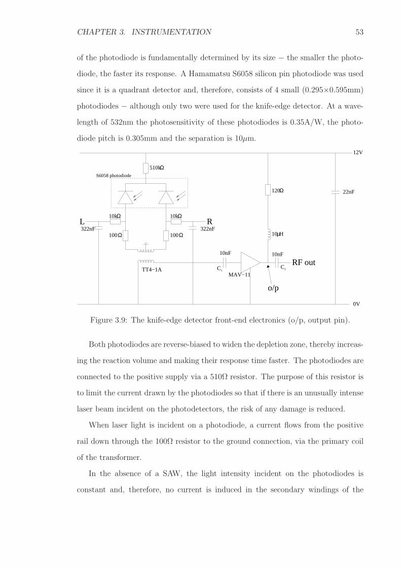
CHAPTER 3. INSTRUMENTATION 53
of the photodiode is fundamentally determined by its size − the smaller the photo-
diode, the faster its response. A Hamamatsu S6058 silicon pin photodiode was used
since it is a quadrant detector and, therefore, consists of 4 small (0.295×0.595mm)
photodiodes − although only two were used for the knife-edge detector. At a wave-
length of 532nm the photosensitivity of these photodiodes is 0.35A/W, the photo-
diode pitch is 0.305mm and the separation is 10µm.
Ω100 100Ω
120Ω
10µH
C1C2
510kΩ
10kΩ10kΩRL
10nF
RF out10nF
22nF
0V
12V
MAV−11
322nF322nF
TT4−1A
S6058 photodiode
o/p
Figure 3.9: The knife-edge detector front-end electronics (o/p, output pin).
Both photodiodes are reverse-biased to widen the depletion zone, thereby increas-
ing the reaction volume and making their response time faster. The photodiodes are
connected to the positive supply via a 510Ω resistor. The purpose of this resistor is
to limit the current drawn by the photodiodes so that if there is an unusually intense
laser beam incident on the photodetectors, the risk of any damage is reduced.
When laser light is incident on a photodiode, a current flows from the positive
rail down through the 100Ω resistor to the ground connection, via the primary coil
of the transformer.
In the absence of a SAW, the light intensity incident on the photodiodes is
constant and, therefore, no current is induced in the secondary windings of the

CHAPTER 3. INSTRUMENTATION 54
transformer. However, a passing SAW causes the reflected beam to oscillate between
the two photodiodes, generating an alternating current in the primary coil of the
transformer. This gives rise to a changing magnetic field, generating a current in
the secondary coil of the transformer. The TT4-1A type transformer being used
here has a useful frequency response from 100kHz to 300MHz.
A MAV-11 monolithic amplifier with a gain of 12.7dB is used to amplify the
output of the transformer. The amplifier is powered through its output pin (o/p
figure 3.9), connected to the supply rail via a 120Ω bias resistor, the value of which
is given by equation 3.3.
Rbias =Vc − Vd
Ibias
(3.3)
where Vc is the supply voltage (12V), Vd and Ibias are the voltage and current values
at the output pin specified to be 5.5V and 60mA, respectively, by the manufacturer.
A 10µH inductor is required to ensure no loss of RF signal due to the bias connection
and that the RF signal on the output does not feedback to the input via the power
rail (since gain is related to Vd), thereby causing oscillation.
Both the input and output pins are connected to capacitors (C1 and C2) to block
any DC. The appropriate capacitor value is chosen for a particular frequency range
of operation. The low frequency cutoff (fc) of the amplifier is given by equation 3.4.
fc =1
2πRC(3.4)
where R is the load impedance on the transformer secondary winding (50Ω) and C
is the value of the capacitor. In terms of frequency range, it is necessary to be able
to detect 0.5MHz SAWs, in which case from equation 3.4, a minimum of 6.4nF is
required. The actual value of the capacitors used was 10nF.
A single resistor and a capacitor are connected to the output of the left and right
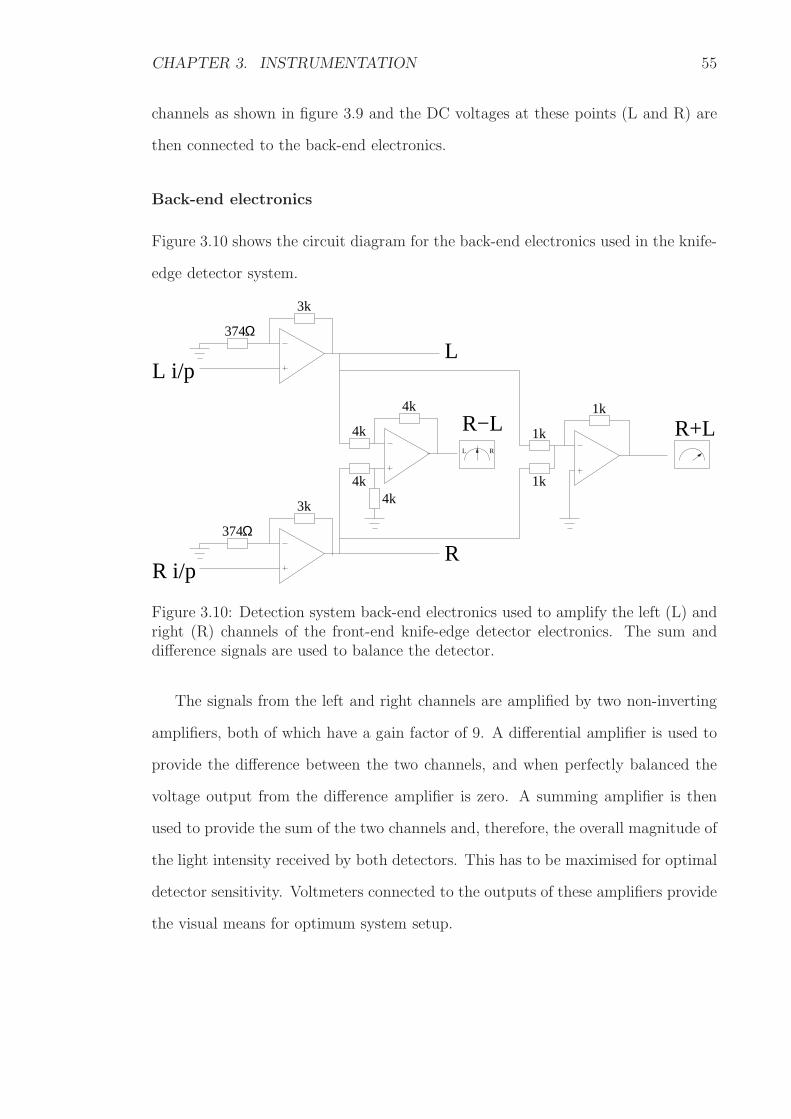
CHAPTER 3. INSTRUMENTATION 55
channels as shown in figure 3.9 and the DC voltages at these points (L and R) are
then connected to the back-end electronics.
Back-end electronics
Figure 3.10 shows the circuit diagram for the back-end electronics used in the knife-
edge detector system.
RL
R
L
R−L R+L
3k
3k
L i/p
R i/p
374Ω
374Ω
4k4k
4k
4k
1k
1k
1k
Figure 3.10: Detection system back-end electronics used to amplify the left (L) andright (R) channels of the front-end knife-edge detector electronics. The sum anddifference signals are used to balance the detector.
The signals from the left and right channels are amplified by two non-inverting
amplifiers, both of which have a gain factor of 9. A differential amplifier is used to
provide the difference between the two channels, and when perfectly balanced the
voltage output from the difference amplifier is zero. A summing amplifier is then
used to provide the sum of the two channels and, therefore, the overall magnitude of
the light intensity received by both detectors. This has to be maximised for optimal
detector sensitivity. Voltmeters connected to the outputs of these amplifiers provide
the visual means for optimum system setup.
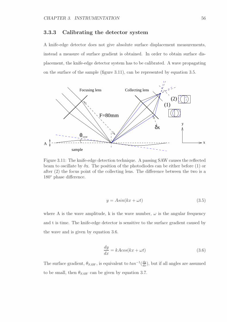
CHAPTER 3. INSTRUMENTATION 56
3.3.3 Calibrating the detector system
A knife-edge detector does not give absolute surface displacement measurements,
instead a measure of surface gradient is obtained. In order to obtain surface dis-
placement, the knife-edge detector system has to be calibrated. A wave propagating
on the surface of the sample (figure 3.11), can be represented by equation 3.5.
xδθSAW
A
Focusing lens Collecting lens
sample
y
x
(2)(1)
F=80mm
Figure 3.11: The knife-edge detection technique. A passing SAW causes the reflectedbeam to oscillate by δx. The position of the photodiodes can be either before (1) orafter (2) the focus point of the collecting lens. The difference between the two is a180 phase difference.
y = Asin(kx+ ωt) (3.5)
where A is the wave amplitude, k is the wave number, ω is the angular frequency
and t is time. The knife-edge detector is sensitive to the surface gradient caused by
the wave and is given by equation 3.6.
dy
dx= kAcos(kx+ ωt) (3.6)
The surface gradient, θSAW , is equivalent to tan−1( dy
dx), but if all angles are assumed
to be small, then θSAW can be given by equation 3.7.
CHAPTER 3. INSTRUMENTATION 57
θSAW ≈dy
dx(3.7)
The sample displacement due to the presence of this SAW causes a change, δx, in
the position of the intensity distribution, as shown in figure 3.11, and is given by
equation 3.8 [52].
δx = 2θSAWF (3.8)
where F is the focal length of the focusing lens shown in figure 3.11. The maximum
deviation of the reflected beam is, therefore, obtained by substituting equation 3.7
into equation 3.8 to give equation 3.9.
δx = 2dy
dxF (3.9)
and substituting 3.6 into 3.9 we obtain equation 3.10
δx = 2kAcos(kx+ ωt)F (3.10)
For maximum surface displacement, δx is equal to 2kAF. Figure 3.12 shows how
the reflected beam deviates from its zero displacement position to the maximum
displacement position. Assuming that the photodiodes are sufficiently large so that
all the light is collected and that there is no space between them, the power drop
observed on one photodiode is equal in magnitude to the power gained by the other.
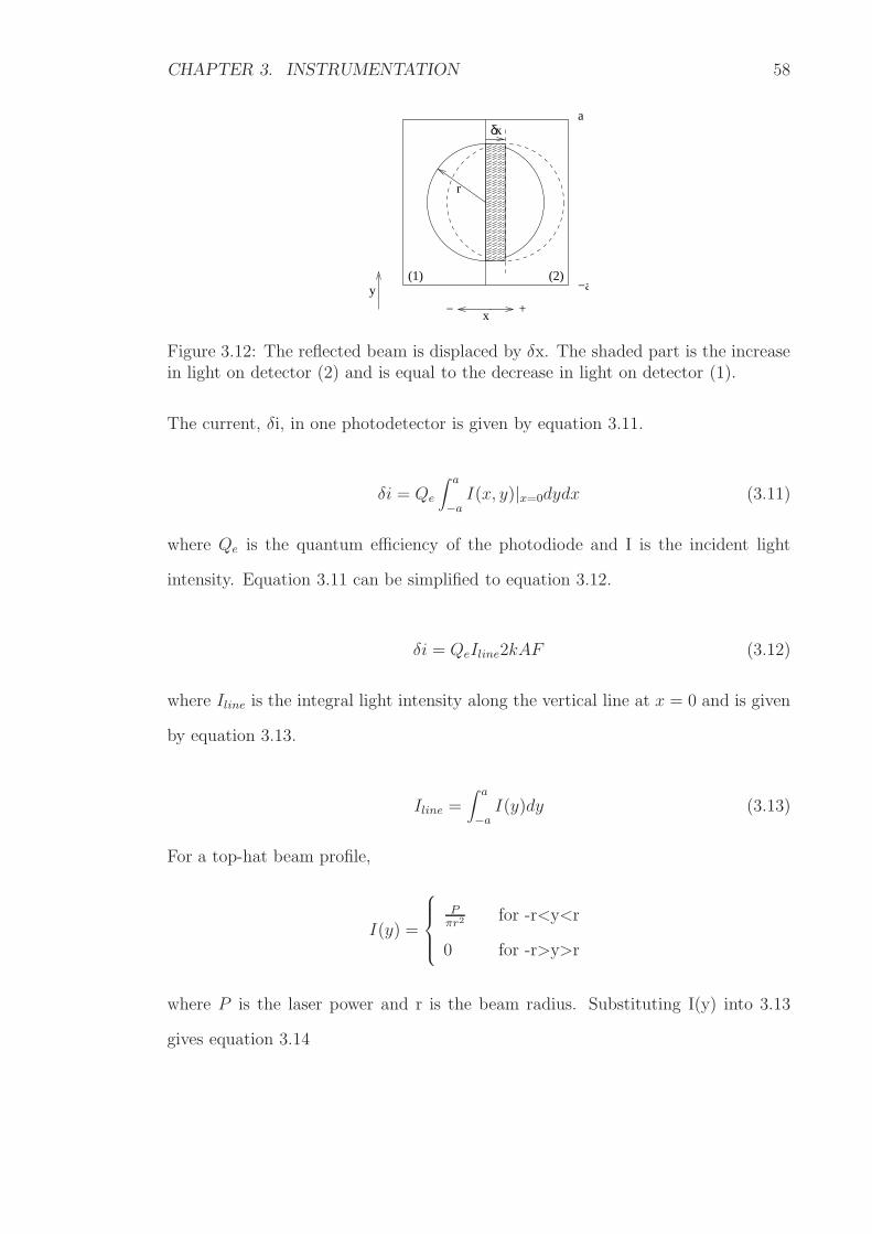
CHAPTER 3. INSTRUMENTATION 58
δx
r
a
−a(1)
x− +
y(2)
Figure 3.12: The reflected beam is displaced by δx. The shaded part is the increasein light on detector (2) and is equal to the decrease in light on detector (1).
The current, δi, in one photodetector is given by equation 3.11.
δi = Qe
∫ a
−aI(x, y)|x=0dydx (3.11)
where Qe is the quantum efficiency of the photodiode and I is the incident light
intensity. Equation 3.11 can be simplified to equation 3.12.
δi = QeIline2kAF (3.12)
where Iline is the integral light intensity along the vertical line at x = 0 and is given
by equation 3.13.
Iline =∫ a
−aI(y)dy (3.13)
For a top-hat beam profile,
I(y) =
Pπr2 for -r<y<r
0 for -r>y>r
where P is the laser power and r is the beam radius. Substituting I(y) into 3.13
gives equation 3.14
CHAPTER 3. INSTRUMENTATION 59
Iline =∫ r
−r
P
πr2dy =
2P
πr=
2P
π(NA)F(3.14)
where NA is the numerical aperture given by NA= rF
. Substituting equation 3.14
into equation 3.12 gives equation 3.15:
δi =4QePAk
π(NA)(3.15)
and substituting k = 2πλ
(where λ is the wavelength of the wave) into 3.15 produces
equation 3.16:
δi =8QePA
λ(NA)(3.16)
The next stage is to determine the DC and AC output voltages of the detector
electronics. Figure 3.13 shows the DC and AC equivalent circuits.
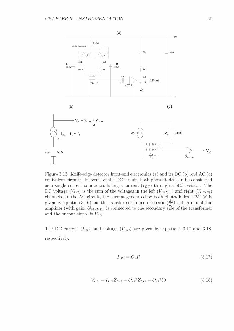
CHAPTER 3. INSTRUMENTATION 60
50Ω
2δi
ZZ
p
s= 4 GMAV11
V = VDC DC(L)+ VDC(R)
I DC I RI L= +
Ω100 100Ω
120Ω
10µH
C1C2
510kΩ
10kΩ10kΩRL
10nF
RF out10nF
22nF
0V
12V
MAV−11
322nF322nF
TT4−1A
S6058 photodiode
o/p
200Ω
VAC
(b) (c)
(a)
DCZ
Zp
2
Figure 3.13: Knife-edge detector front-end electronics (a) and its DC (b) and AC (c)equivalent circuits. In terms of the DC circuit, both photodiodes can be consideredas a single current source producing a current (IDC) through a 50Ω resistor. TheDC voltage (VDC) is the sum of the voltages in the left (VDC(L)) and right (VDC(R))channels. In the AC circuit, the current generated by both photodiodes is 2δi (δi isgiven by equation 3.16) and the transformer impedance ratio (Zp
Zs
) is 4. A monolithicamplifier (with gain, GMAV 11) is connected to the secondary side of the transformerand the output signal is VAC .
The DC current (IDC) and voltage (VDC) are given by equations 3.17 and 3.18,
respectively.
IDC = QeP (3.17)
VDC = IDCZDC = QePZDC = QeP50 (3.18)
CHAPTER 3. INSTRUMENTATION 61
where ZDC is the resistance in the DC equivalent circuit. The impedance ratio
(Zp
Zs
) of the transformer is 4 and is, therefore, equivalent to a voltage ratio of 2.
The voltages across the primary windings (Vp) and secondary windings (Vs) of the
transformer are given by equations 3.19 and 3.20, respectively.
Vp = 2δiZp = 2δi200 (3.19)
Vs =Vp
2= δiZp = δi200 (3.20)
where Zp is 200Ω (figure 3.13(c)). The AC voltage (VAC) is given by equation 3.21:
VAC = VsGMAV 11 = 200δiGMAV 11 (3.21)
where GMAV 11 is the gain of the MAV-11 amplifier shown in figure 3.13(a). Substi-
tuting equation 3.16 into equation 3.21, we obtain equation 3.22
VAC =1600QePAGMAV 11
λ(NA)(3.22)
rearranging equation 3.18 for P and substituting into 3.22, generates equation 3.23
VAC =32VDCAGMAV 11
λ(NA)(3.23)
Rearranging equation 3.23 for A, we obtain equation 3.24:
A =VAC
VDC
λ(NA)
32GMAV 11(3.24)
Equation 3.24 relates the surface displacement (A) to the output voltages from the
front-end electronics (VAC and VDC). To complete the calibration of the detector
system, the gains in the AC and DC output paths have to be considered. The
complete detector system is shown in figure 3.14.
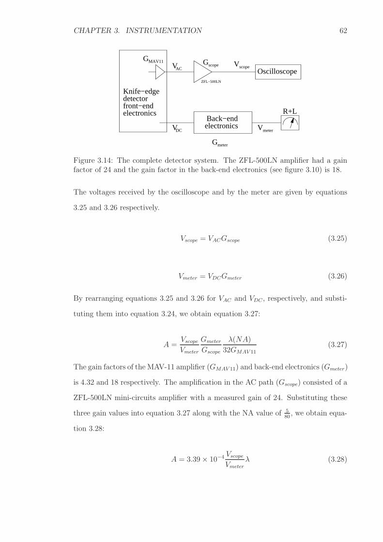
CHAPTER 3. INSTRUMENTATION 62
VAC
Vmeter
Vscope
GMAV11
Knife−edgedetectorfront−endelectronics
Back−endelectronics
DCV
Gscope
Gmeter
ZFL−500LN
R+L
Oscilloscope
Figure 3.14: The complete detector system. The ZFL-500LN amplifier had a gainfactor of 24 and the gain factor in the back-end electronics (see figure 3.10) is 18.
The voltages received by the oscilloscope and by the meter are given by equations
3.25 and 3.26 respectively.
Vscope = VACGscope (3.25)
Vmeter = VDCGmeter (3.26)
By rearranging equations 3.25 and 3.26 for VAC and VDC , respectively, and substi-
tuting them into equation 3.24, we obtain equation 3.27:
A =Vscope
Vmeter
Gmeter
Gscope
λ(NA)
32GMAV 11
(3.27)
The gain factors of the MAV-11 amplifier (GMAV 11) and back-end electronics (Gmeter)
is 4.32 and 18 respectively. The amplification in the AC path (Gscope) consisted of a
ZFL-500LN mini-circuits amplifier with a measured gain of 24. Substituting these
three gain values into equation 3.27 along with the NA value of 580
, we obtain equa-
tion 3.28:
A = 3.39 × 10⁻⁴ Vscope
Vmeter
λ (3.28)
CHAPTER 3. INSTRUMENTATION 63
Equation 3.28 was readily used for the results presented in Chapter 5.
3.4 CHOT system configuration
In addition to performing nonlinear experiments using the OSAM, CHOTs provided
an alternative method of generating and detecting ultrasound [94]. This section
describes the CHOTs that were specifically integrated into the nonlinear experiments
described in section 4.4.
3.4.1 g-CHOT
A fused silica substrate was used for this nonlinear experimental work. Using pho-
tolithography, a g-CHOT, made up of multiple lines of titanium, was deposited on
the sample. The efficiency of the g-CHOT was dependent on the absorption contrast
between the substrate and the deposited material. The layer of titanium deposited
was ∼146nm thick and the lines were equally spaced, which provided a periodic ab-
sorption contrast between the coated and non-coated areas of the substrate. When
the incident laser beam was used to activate the g-CHOT, the titanium absorbed
the radiation more strongly than the transparent fused silica substrate. Based on
published reflection and transmission coefficients [95], it is estimated that 76% of the
incident light radiation was reflected, 20% was transmitted and 4% was absorbed by
the thin titanium layer. In contrast, the fused silica substrate transmitted 96% of
the radiation through its 6mm thickness (according to the manufacturer), while 3%
of it was reflected. The titanium coated parts of the fused silica experienced local
thermal expansion, whereas the uncoated regions did not. The difference in local
expansion when illuminated by a pulsed laser caused the generation of an elastic
wave. Even though the absorption contrast between the g-CHOT pattern and the
substrate was only 4%, it was still sufficient to generate detectable ultrasound.
CHAPTER 3. INSTRUMENTATION 64
Selecting appropriate line spacing
The line spacing was selected to match the acoustic wavelength of the ultrasound
to be generated on the inspected material using λSAW=v/f : where λSAW is the
acoustic wavelength (line spacing), v is the Rayleigh wave velocity and f is the
frequency of the SAW. If the g-CHOT is activated by a laser containing a broad
frequency spectrum, then the CHOT is designed to actively select any frequency
within the bandwidth of the laser, and the outcome of this is narrowband-generated
ultrasound. However, in this work the g-CHOT was activated by a Q-switched and
mode-locked Nd:YAG laser. The output frequency spectrum from this source was
narrowband with a fundamental frequency of 82MHz. This meant that the line
spacing of the g-CHOT had to match the acoustic wavelength at 82MHz on the
material. In order to accurately obtain the appropriate wavelength of a material
(i.e. fused silica) with an unknown velocity, a ‘λ-scan’ was performed by the OSAM
instrument prior to CHOT fabrication to measure the line spacing (figure 3.15).
During this experiment, the SLM was programmed to adjust the line spacing and
the 82MHz signal was detected by the knife-edge detector. The magnitude of the
82MHz frequency component was then plotted (figure 3.15). The 82MHz frequency
component was most efficiently generated when the SLM line spacing was 41.7µm,
which corresponded to a velocity of 3419ms−1. For the experiments presented in
this chapter, the actual spacing of the fabricated g-CHOT was 41µm.
Imaging ultrasound generated by the g-CHOT
Using the high-speed analogue electronics that were described in section 3.5, it was
possible to image the generated ultrasonic field. This was achieved by raster scanning
the knife-edge detector over the sample surface, and obtaining the amplitude and
phase information of the detected signal at each point in the scan. The image that
this produced is termed an aerial PSF. Figure 3.16 shows aerial PSFs obtained for
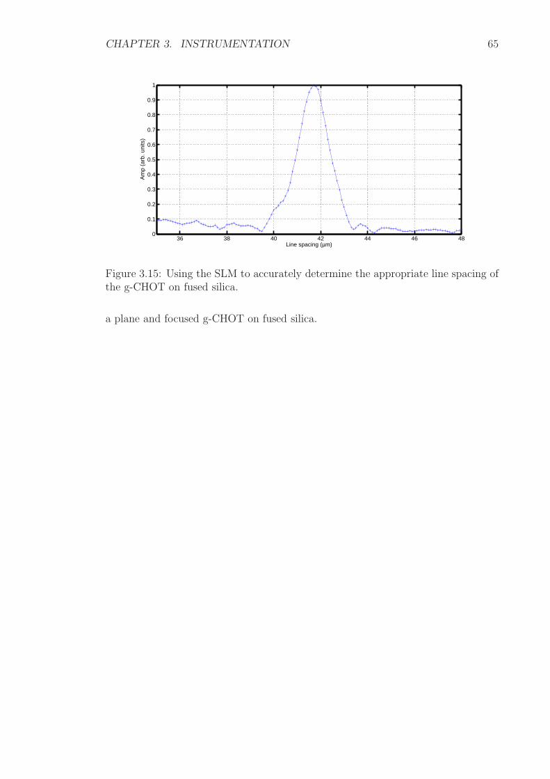
CHAPTER 3. INSTRUMENTATION 65
36 38 40 42 44 46 480
0.1
0.2
0.3
0.4
0.5
0.6
0.7
0.8
0.9
1
Line spacing (µm)
Am
p (a
rb. u
nits
)
Figure 3.15: Using the SLM to accurately determine the appropriate line spacing ofthe g-CHOT on fused silica.
a plane and focused g-CHOT on fused silica.

CHAPTER 3. INSTRUMENTATION 66
µm
µm
−500 0 500
500
0
−500
−500
050
00
0.2
0.4
0.6
0.81
Amp (arb units)
posi
tion
(µm
)−5
000
500
0
0.2
0.4
0.6
0.81
posi
tion
(µm
)
Amp (arb units)µm
µm
−500 0 500
500
0
−500
(b)
(a)
Figure 3.16: Aerial PSF from a plane (a) and focused (b) g-CHOT on fused silica.The knife-edge detector was scanned in 10µm steps over the sample surface. Theplane wave g-CHOT was made up of titanium lines, while the focused g-CHOTstructure was composed of deposited aluminium lines.

CHAPTER 3. INSTRUMENTATION 67
3.4.2 d-CHOT
The d-CHOT was made by evaporating an initial layer of silver (∼140nm) to make
the sample surface reflective and then fabricating the lines using photolithography.
The second deposited layer of silver created steps of ∼82nm in height. The step
height was dependent on the incident angle of the laser beam (relative to the sample
surface) and for the experiment presented in this work, the incident angle was 45.
According to equation 1.21, the steps should be 94nm in height for optimum opera-
tion at 45 incidence angle. Therefore, although the experiment was not operating
at 100% optimum conditions, the reduction in efficiency was small and estimated to
be 0.99 of the optimum value.
Optical configuration
For the nonlinear experiments performed in this work, a frequency doubled 532nm
Nd:YAG CW laser was used at an incident angle of 45 relative to the sample surface.
The d-CHOT was activated by focusing the detector laser beam to a 2mm spot using
a combination of two lenses shown in figure 3.17.
Detectorlaser photodiode
Single
F=40
F=10 F=10
F=40LL
LL I
Sample
Figure 3.17: Basic optical configuration required for the activation of the d-CHOT.L=lens, fl=focal length (mm), I=iris.
The light power at the sample surface was measured to be 30mW. The reflected
beam was split into several diffractive orders by the d-CHOT and an iris was used
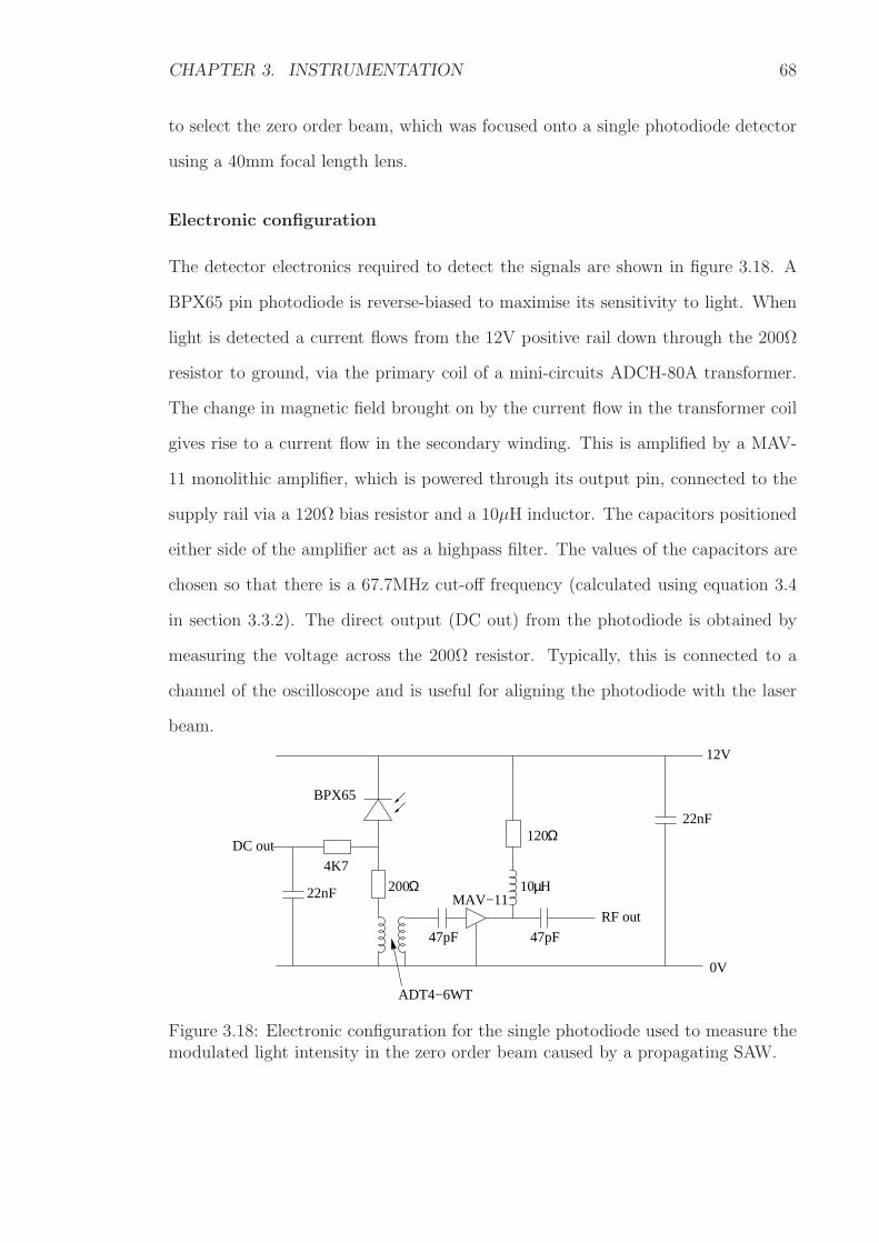
CHAPTER 3. INSTRUMENTATION 68
to select the zero order beam, which was focused onto a single photodiode detector
using a 40mm focal length lens.
Electronic configuration
The detector electronics required to detect the signals are shown in figure 3.18. A
BPX65 pin photodiode is reverse-biased to maximise its sensitivity to light. When
light is detected a current flows from the 12V positive rail down through the 200Ω
resistor to ground, via the primary coil of a mini-circuits ADCH-80A transformer.
The change in magnetic field brought on by the current flow in the transformer coil
gives rise to a current flow in the secondary winding. This is amplified by a MAV-
11 monolithic amplifier, which is powered through its output pin, connected to the
supply rail via a 120Ω bias resistor and a 10µH inductor. The capacitors positioned
either side of the amplifier act as a highpass filter. The values of the capacitors are
chosen so that there is a 67.7MHz cut-off frequency (calculated using equation 3.4
in section 3.3.2). The direct output (DC out) from the photodiode is obtained by
measuring the voltage across the 200Ω resistor. Typically, this is connected to a
channel of the oscilloscope and is useful for aligning the photodiode with the laser
beam.
200Ω
120Ω
10µH
47pF 47pF
MAV−11RF out
DC out
22nF
12V
0V
22nF
4K7
ADT4−6WT
BPX65
Figure 3.18: Electronic configuration for the single photodiode used to measure themodulated light intensity in the zero order beam caused by a propagating SAW.

CHAPTER 3. INSTRUMENTATION 69
3.5 High-speed data acquisition − the analogue
electronics
The electronics that are used for the high-speed data acquisition have been described
previously in [93], and will be summarised in this section. The purpose of this
electronic system is to acquire the amplitude and phase information of the detected
ultrasound on the sample at high-speed.
Specifically, ‘phase’ refers to the difference between the 82MHz components of the
detected and reference signals. This system is able to acquire information rapidly,
making it useful for producing c-scans and aerial PSFs. In order to acquire the
amplitude and phase information, there are three required inputs to the system
figure 3.19:
1. Detected signal by the knife-edge detector.
2. The coherent trigger pulse.
3. A reference 41MHz signal.
+90
10MHzLPF
Sample andhold
LPF
A/D
Trigger pulse
Doubler
(41MHz)Mode−locker
Peak detector
Peak detectordetector
Knife−edge
realV
Vimag
10MHzhold
Sample and imag
real
Figure 3.19: Diagram of the analogue electronics required for high-speed data ac-quisition.
A 41MHz reference signal derived from the mode-locker (and coherent with the
laser pulses) is doubled and then mixed with the detected signal from the knife-edge
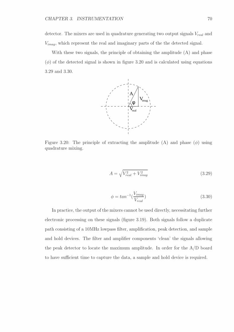
CHAPTER 3. INSTRUMENTATION 70
detector. The mixers are used in quadrature generating two output signals Vreal and
Vimag, which represent the real and imaginary parts of the the detected signal.
With these two signals, the principle of obtaining the amplitude (A) and phase
(φ) of the detected signal is shown in figure 3.20 and is calculated using equations
3.29 and 3.30.
V
Vreal
imag
A
φ
Figure 3.20: The principle of extracting the amplitude (A) and phase (φ) usingquadrature mixing.
A =√
V 2real + V 2
imag (3.29)
φ = tan−1(Vimag
Vreal
) (3.30)
In practice, the output of the mixers cannot be used directly, necessitating further
electronic processing on these signals (figure 3.19). Both signals follow a duplicate
path consisting of a 10MHz lowpass filter, amplification, peak detection, and sample
and hold devices. The filter and amplifier components ‘clean’ the signals allowing
the peak detector to locate the maximum amplitude. In order for the A/D board
to have sufficient time to capture the data, a sample and hold device is required.
CHAPTER 3. INSTRUMENTATION 71
3.6 Summary
The generation system used in the OSAM instrument consists of a Q-switched and
mode-locked IR laser and a SLM. The fundamental frequency of the generated SAWs
is 82MHz, but generating SAWs at the harmonics of 82MHz is possible. Detections
of SAWs is performed using a knife-edge detector system. For reference purposes, a
guide to aligning the OSAM instrument is included in Appendix C.
The calibration of the detection system has meant that surface displacement can
be obtained and from this the stress exerted by the pump SAW can be acquired.
The velocity modulation experienced by the probe SAW is presented with respect
to surface stress (see Chapter 5). The relationship between stress and velocity
modulation provides the measure of material nonlinearity.
Chapter 4
Experimental Method
4.1 Introduction
The OSAM instrument had to be adapted for the integration of the nonlinear ex-
periments. The following three modifications had to be made.
1. A low frequency (‘pump’) SAW generation system was integrated.
2. Accurate timing electronics were required to control the relative triggering
times of the pump and probe SAWs.
3. The effects of temperature variation had to be suppressed.
Since the experiment relies on adjusting the point at which two SAWs interact
with each other, an accurate timing control system was constructed to delay the
triggering of one source of ultrasound with respect to another. Although this system
could set the delay to within an 8ns accuracy but there were additional, albeit
relatively minor contributions of timing jitter from other experimental apparatus.
A more significant source of noise compared with the timing jitter was due to
changes in ambient temperature in the laboratory. During the course of this work,
it was found that velocity variations due to temperature changes were of the same
72

CHAPTER 4. EXPERIMENTAL METHOD 73
order to the those caused by material nonlinearity. It was crucial to the success
of these experiments to minimise the effect of temperature. Two techniques were
used to achieve this. Firstly, a highly stable temperature controlled environment was
designed and constructed, capable of maintaining the air temperature around certain
elements of the experimental apparatus to within ∼0.01C. Secondly, an adapted
data collection technique was developed that suppressed the effect of temperature,
typically by a factor of 200.
4.2 Experimental aim and concept
The experiment aimed to measure material nonlinearity by observing a velocity
change caused by an applied stress, induced by a low frequency (‘pumping’) SAW
packet in the frequency range 0.5−2MHz. Figure 4.1 shows the stress imposed by a
1MHz wave packet on an aluminium-2024 sample.
The stress exerted by the transducer was calculated by first calibrating the knife-
edge detector to acquire the displacement and then using the analysis reviewed in
section 1.4.2, to determine the stress. The material properties for aluminium-2024
used in the analysis are shown in Appendix A.
The sample surface experienced maximum stresses at points A and B and zero
stress at point C. Previous experiments have shown that applied stress influences the
velocity of ultrasound [13]. If a second (‘probing’) SAW interacted with the pump
SAW at positions A, B and C, then the probe SAW would experience a velocity shift
depending on these stress levels. The point of interaction between the two SAWs
was achieved by delaying the triggering time of the probe relative to the pump.
Figure 4.2 is a trace of a typical probe pulse. The probe pulse envelope had
a full-wave-at-half-maximum (FWHM) of 0.4µs and, therefore, instead of seeing
a discrete stress level (as figure 4.1 indicates), it actually experienced a range of
stresses (over its entire duration) exerted by the pump SAW − approximately 40%

CHAPTER 4. EXPERIMENTAL METHOD 74
0 1 2 3 4 5 6 7 8−4
−3
−2
−1
0
1
2
3
4
Str
ess
(MP
a)
Time (µs)
A
C
B
Figure 4.1: Surface stress induced by a 3-cycle SAW generated by a 1MHz transduceron an aluminium-2024 sample. The stress experienced by the probe SAW dependson its point of interaction with the pump − three interaction positions are labelledA, B and C.
of a 1MHz pump cycle. Despite this, it was still possible to measure the velocity
shift experienced by the probe. The experimental measurements were, therefore, an
‘averaged’ result over the portion of the pump wave that the probe interacted with.
By using a lower frequency transducer, the stress range experienced by the probe
pulse would be reduced.
In a truly linear sample, the velocity of the probe pulse would not change with
induced stress, i.e. there would be no interaction between the pump and probe
waves. In reality, all materials exhibit nonlinearity to a greater or lesser extent
depending on their elastic properties.
4.3 Nonlinear experiment configuration
The essential elements of the experimental apparatus that have not yet been dis-
cussed are shown in figure 4.3.
A typical interaction distance (also referred to as the arc focal length) for the

CHAPTER 4. EXPERIMENTAL METHOD 75
0 0.1 0.2 0.3 0.4 0.5 0.6 0.7 0.8 0.9−1
−0.5
0
0.5
1
Time(µs)
Am
plitu
de (
arb.
uni
ts)
Figure 4.2: Detected probe pulse SAW generated by a Q-switched mode-locked laserand SLM. The experiment required accurate timing so that this signal interactedwith various points on the pump SAW packet. By extracting the phase responsefrom this signal at each of these interaction points, there was a direct measure ofvelocity change with respect to surface stress.
pump and probe SAWs was 4mm and this was strictly taken to be the distance
between the centre of the SLM image and the detection point.
The measured phase difference is proportional to the pump/probe interaction
distance, and therefore an improved nonlinear measurement would be obtained at
longer distances. However, the optimal distance is limited by the SAW detectability
(SNR) because the amplitude is diminished by attenuation and aberration. Poor
SNR can be overcome by averaging, but this increases the acquisition time of each
experiment. Since material aberration is a factor that can limit the interaction
distance, correction methods [96], could be incorporated into the experiment to
compensate for these effects.
If the interaction distance is very short, the measurement of material nonlinearity
is made difficult because the instrumentation would be unable to resolve the very
small phase changes in the probe signal. Taking these factors into consideration,
an interaction distance of 4mm was appropriate for the fused silica and aluminium
samples used in this thesis.
The knife-edge detection system was sensitive to both the pump and probe SAW
frequencies. The overall bandwidth of the detector was within a 100kHz to the GHz
frequency range. A custom made 82MHz bandpass filter was used (TVC incorpo-
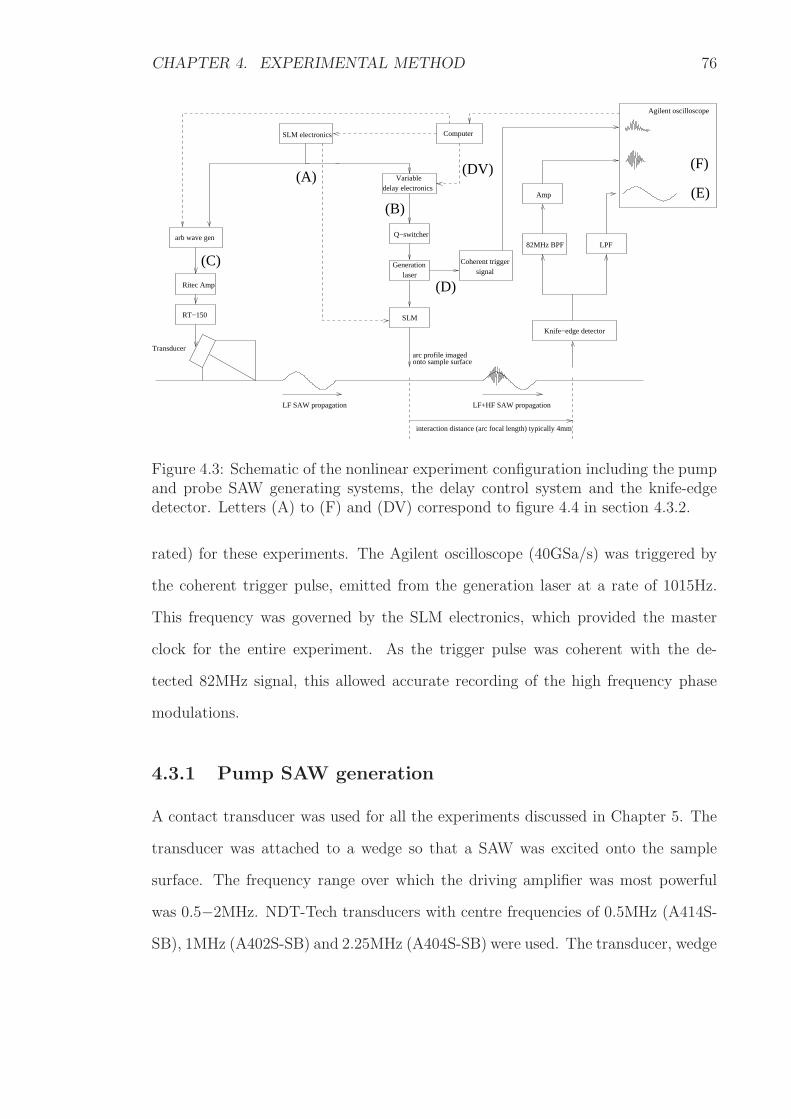
CHAPTER 4. EXPERIMENTAL METHOD 76
Ritec Amp
SLM electronics
Amp
arc profile imagedonto sample surface
LF+HF SAW propagationLF SAW propagation
interaction distance (arc focal length) typically 4mm
82MHz BPF LPF
Transducer
RT−150
(DV)Variable
delay electronics (E)
signalCoherent trigger
laserGeneration
arb wave gen
Agilent oscilloscope
Computer
SLM
Q−switcher
(C)
(A)
(B)
(D)
(F)
Knife−edge detector
Figure 4.3: Schematic of the nonlinear experiment configuration including the pumpand probe SAW generating systems, the delay control system and the knife-edgedetector. Letters (A) to (F) and (DV) correspond to figure 4.4 in section 4.3.2.
rated) for these experiments. The Agilent oscilloscope (40GSa/s) was triggered by
the coherent trigger pulse, emitted from the generation laser at a rate of 1015Hz.
This frequency was governed by the SLM electronics, which provided the master
clock for the entire experiment. As the trigger pulse was coherent with the de-
tected 82MHz signal, this allowed accurate recording of the high frequency phase
modulations.
4.3.1 Pump SAW generation
A contact transducer was used for all the experiments discussed in Chapter 5. The
transducer was attached to a wedge so that a SAW was excited onto the sample
surface. The frequency range over which the driving amplifier was most powerful
was 0.5−2MHz. NDT-Tech transducers with centre frequencies of 0.5MHz (A414S-
SB), 1MHz (A402S-SB) and 2.25MHz (A404S-SB) were used. The transducer, wedge

CHAPTER 4. EXPERIMENTAL METHOD 77
and sample were bonded together with Phenyl salicylate.
The transducer selection was based on its ability to accept high voltage inputs
and, therefore, the generation of large displacements (of the order of 20-100nm).
Factors such as element size and shape were less important considerations, as the
purpose of the transducer was simply to stress the surface of the sample.
The transducer driving signal was generated by the Agilent 33250A arbitrary
waveform generator. This device was externally triggered by the timing electronics,
and on each trigger event a 3-cycle sine wave with a peak-to-peak amplitude in the
range of 0−0.65V was generated.
This signal was amplified by a Ritec RPR-4000 gated amplifier, which had a
gain of 100dB and a peak output power of 8kW. Maximum input voltages to the
transducer were 1400V.
4.3.2 Timing setup
The overall ‘speed’ of the experiment was dictated by the repetition rate of the SLM
and laser, which was 1015Hz. The digital signal that was generated by the SLM
electronics is (by tradition) known as the T/I (true/inverse) signal and this provided
the master clock for the entire apparatus (figure 4.4). The T/I signal was a square
wave with a duty cycle of 0.5 and a peak voltage of 5V.
The T/I signal was split (A) and the arbitrary waveform generator was triggered
directly by its negative-going edge. This then generated a 3-cycle burst (C) at an
appropriate frequency for the transducer. The delay electronics also received the
T/I signal and generated a new digital signal, referred to as the ‘laser trigger signal’
(B). The electronics consisted of a Spartan 3 Xilinx field programmable gate array
(FPGA) board, which was programmed using VHDL code to count down from a
given number or ‘delay value’ (DV), determined by the computer. When the count
reached zero, it produced a positive edge in the laser trigger signal that triggered the

CHAPTER 4. EXPERIMENTAL METHOD 78
Laser triggersignal
Laser triggersignal
Detectedsignals
A E F
DB
C
electronicsSLM DetectorSample
SLMQ−switcherLaserDelay
electronics
DV
Sig. gen. Amp Transducer
T/I
T/I
d
1ms
Φ
(A)
(B)
(C)
(D)
(E)
(F)
(A)
(B)
(C)
(D)
(E)
(F)
(DV)
Figure 4.4: Timing setup of the experiment. The SLM electronics generated the T/Idigital signal (A) which was used to trigger the signal generator (directly) and alsothe delay electronics. A delay value (DV) from the computer was used to adjust thetime (d) at which the laser was triggered (B) with respect to the signal generator(C). The laser generated a coherent trigger pulse (D) to trigger the oscilloscope.The pump (E) and probe (F) SAWs were then detected and the phase (Φ) of theprobe pulse was extracted.
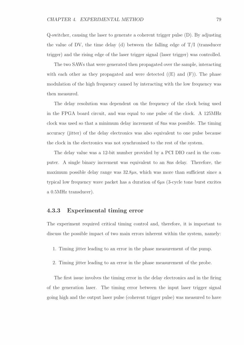
CHAPTER 4. EXPERIMENTAL METHOD 79
Q-switcher, causing the laser to generate a coherent trigger pulse (D). By adjusting
the value of DV, the time delay (d) between the falling edge of T/I (transducer
trigger) and the rising edge of the laser trigger signal (laser trigger) was controlled.
The two SAWs that were generated then propagated over the sample, interacting
with each other as they propagated and were detected ((E) and (F)). The phase
modulation of the high frequency caused by interacting with the low frequency was
then measured.
The delay resolution was dependent on the frequency of the clock being used
in the FPGA board circuit, and was equal to one pulse of the clock. A 125MHz
clock was used so that a minimum delay increment of 8ns was possible. The timing
accuracy (jitter) of the delay electronics was also equivalent to one pulse because
the clock in the electronics was not synchronised to the rest of the system.
The delay value was a 12-bit number provided by a PCI DIO card in the com-
puter. A single binary increment was equivalent to an 8ns delay. Therefore, the
maximum possible delay range was 32.8µs, which was more than sufficient since a
typical low frequency wave packet has a duration of 6µs (3-cycle tone burst excites
a 0.5MHz transducer).
4.3.3 Experimental timing error
The experiment required critical timing control and, therefore, it is important to
discuss the possible impact of two main errors inherent within the system, namely:
1. Timing jitter leading to an error in the phase measurement of the pump.
2. Timing jitter leading to an error in the phase measurement of the probe.
The first issue involves the timing error in the delay electronics and in the firing
of the generation laser. The timing error between the input laser trigger signal
going high and the output laser pulse (coherent trigger pulse) was measured to have
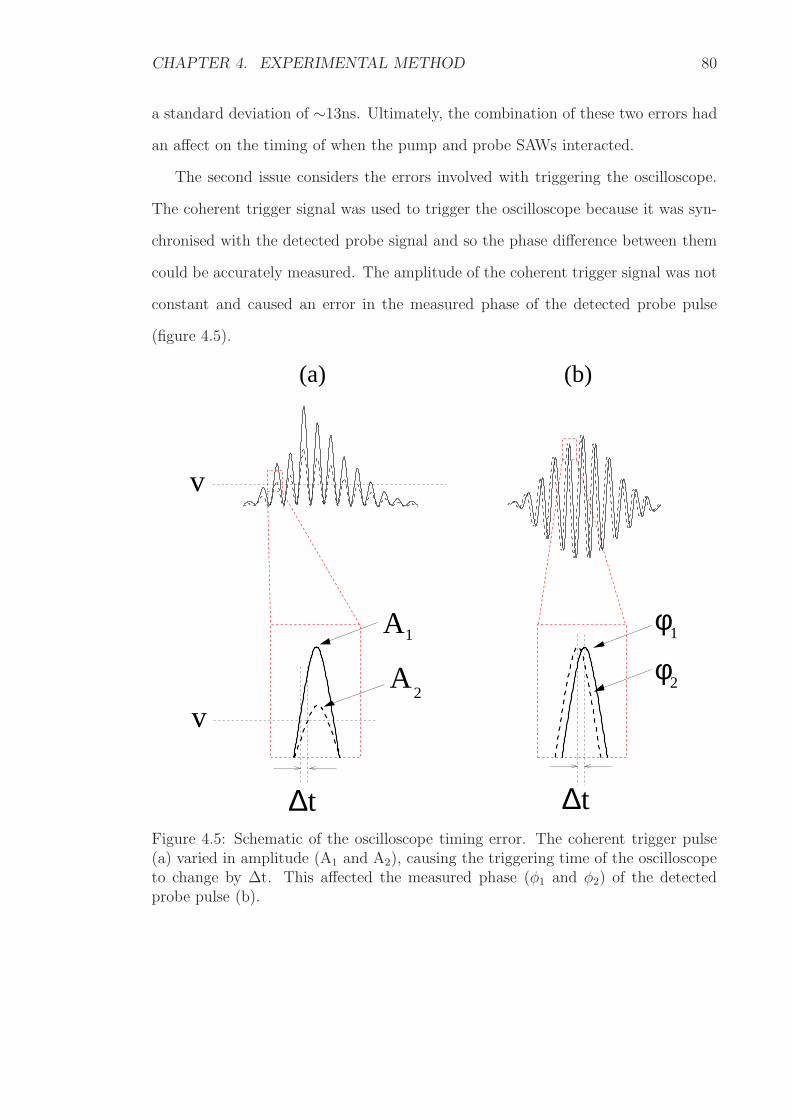
CHAPTER 4. EXPERIMENTAL METHOD 80
a standard deviation of ∼13ns. Ultimately, the combination of these two errors had
an affect on the timing of when the pump and probe SAWs interacted.
The second issue considers the errors involved with triggering the oscilloscope.
The coherent trigger signal was used to trigger the oscilloscope because it was syn-
chronised with the detected probe signal and so the phase difference between them
could be accurately measured. The amplitude of the coherent trigger signal was not
constant and caused an error in the measured phase of the detected probe pulse
(figure 4.5).
A2
A φ1
φ2
(b)
t∆
v
∆t
v
(a)
1
Figure 4.5: Schematic of the oscilloscope timing error. The coherent trigger pulse(a) varied in amplitude (A1 and A2), causing the triggering time of the oscilloscopeto change by ∆t. This affected the measured phase (φ1 and φ2) of the detectedprobe pulse (b).
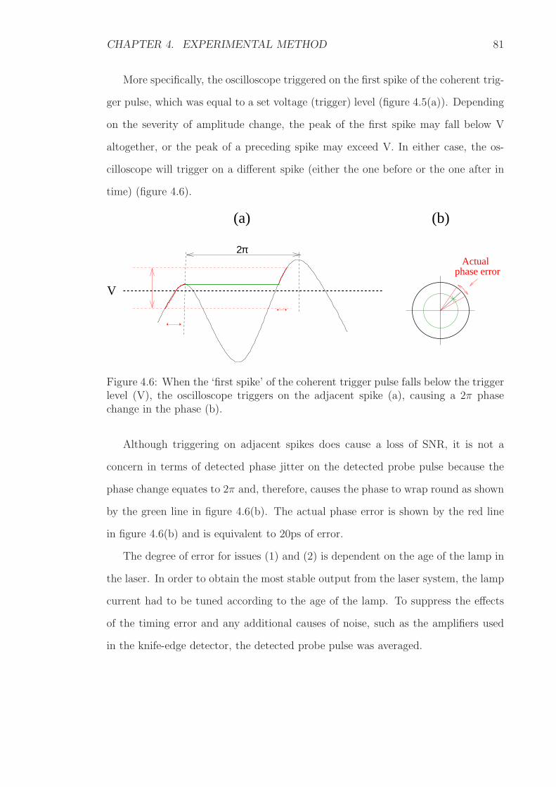
CHAPTER 4. EXPERIMENTAL METHOD 81
More specifically, the oscilloscope triggered on the first spike of the coherent trig-
ger pulse, which was equal to a set voltage (trigger) level (figure 4.5(a)). Depending
on the severity of amplitude change, the peak of the first spike may fall below V
altogether, or the peak of a preceding spike may exceed V. In either case, the os-
cilloscope will trigger on a different spike (either the one before or the one after in
time) (figure 4.6).
V
2π
(a) (b)
Actualphase error
Figure 4.6: When the ‘first spike’ of the coherent trigger pulse falls below the triggerlevel (V), the oscilloscope triggers on the adjacent spike (a), causing a 2π phasechange in the phase (b).
Although triggering on adjacent spikes does cause a loss of SNR, it is not a
concern in terms of detected phase jitter on the detected probe pulse because the
phase change equates to 2π and, therefore, causes the phase to wrap round as shown
by the green line in figure 4.6(b). The actual phase error is shown by the red line
in figure 4.6(b) and is equivalent to 20ps of error.
The degree of error for issues (1) and (2) is dependent on the age of the lamp in
the laser. In order to obtain the most stable output from the laser system, the lamp
current had to be tuned according to the age of the lamp. To suppress the effects
of the timing error and any additional causes of noise, such as the amplifiers used
in the knife-edge detector, the detected probe pulse was averaged.
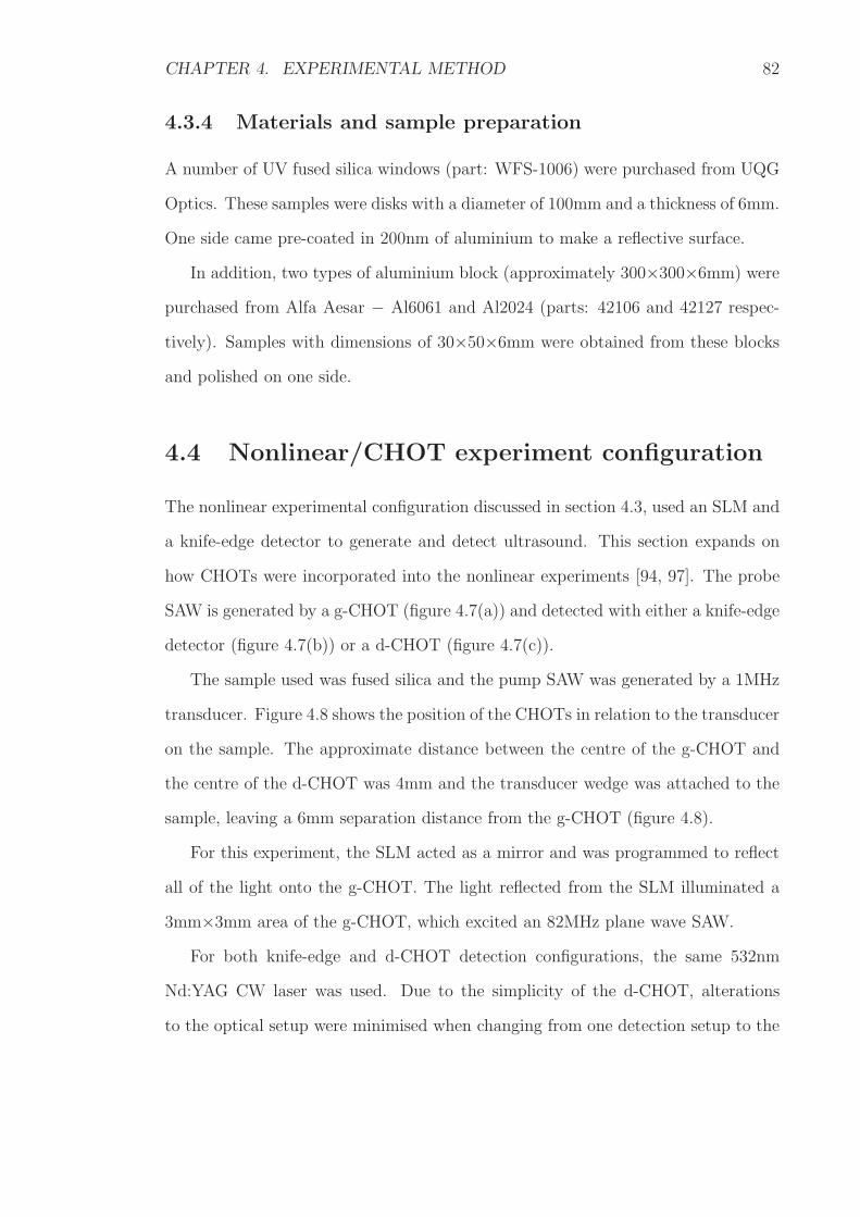
CHAPTER 4. EXPERIMENTAL METHOD 82
4.3.4 Materials and sample preparation
A number of UV fused silica windows (part: WFS-1006) were purchased from UQG
Optics. These samples were disks with a diameter of 100mm and a thickness of 6mm.
One side came pre-coated in 200nm of aluminium to make a reflective surface.
In addition, two types of aluminium block (approximately 300×300×6mm) were
purchased from Alfa Aesar − Al6061 and Al2024 (parts: 42106 and 42127 respec-
tively). Samples with dimensions of 30×50×6mm were obtained from these blocks
and polished on one side.
4.4 Nonlinear/CHOT experiment configuration
The nonlinear experimental configuration discussed in section 4.3, used an SLM and
a knife-edge detector to generate and detect ultrasound. This section expands on
how CHOTs were incorporated into the nonlinear experiments [94, 97]. The probe
SAW is generated by a g-CHOT (figure 4.7(a)) and detected with either a knife-edge
detector (figure 4.7(b)) or a d-CHOT (figure 4.7(c)).
The sample used was fused silica and the pump SAW was generated by a 1MHz
transducer. Figure 4.8 shows the position of the CHOTs in relation to the transducer
on the sample. The approximate distance between the centre of the g-CHOT and
the centre of the d-CHOT was 4mm and the transducer wedge was attached to the
sample, leaving a 6mm separation distance from the g-CHOT (figure 4.8).
For this experiment, the SLM acted as a mirror and was programmed to reflect
all of the light onto the g-CHOT. The light reflected from the SLM illuminated a
3mm×3mm area of the g-CHOT, which excited an 82MHz plane wave SAW.
For both knife-edge and d-CHOT detection configurations, the same 532nm
Nd:YAG CW laser was used. Due to the simplicity of the d-CHOT, alterations
to the optical setup were minimised when changing from one detection setup to the
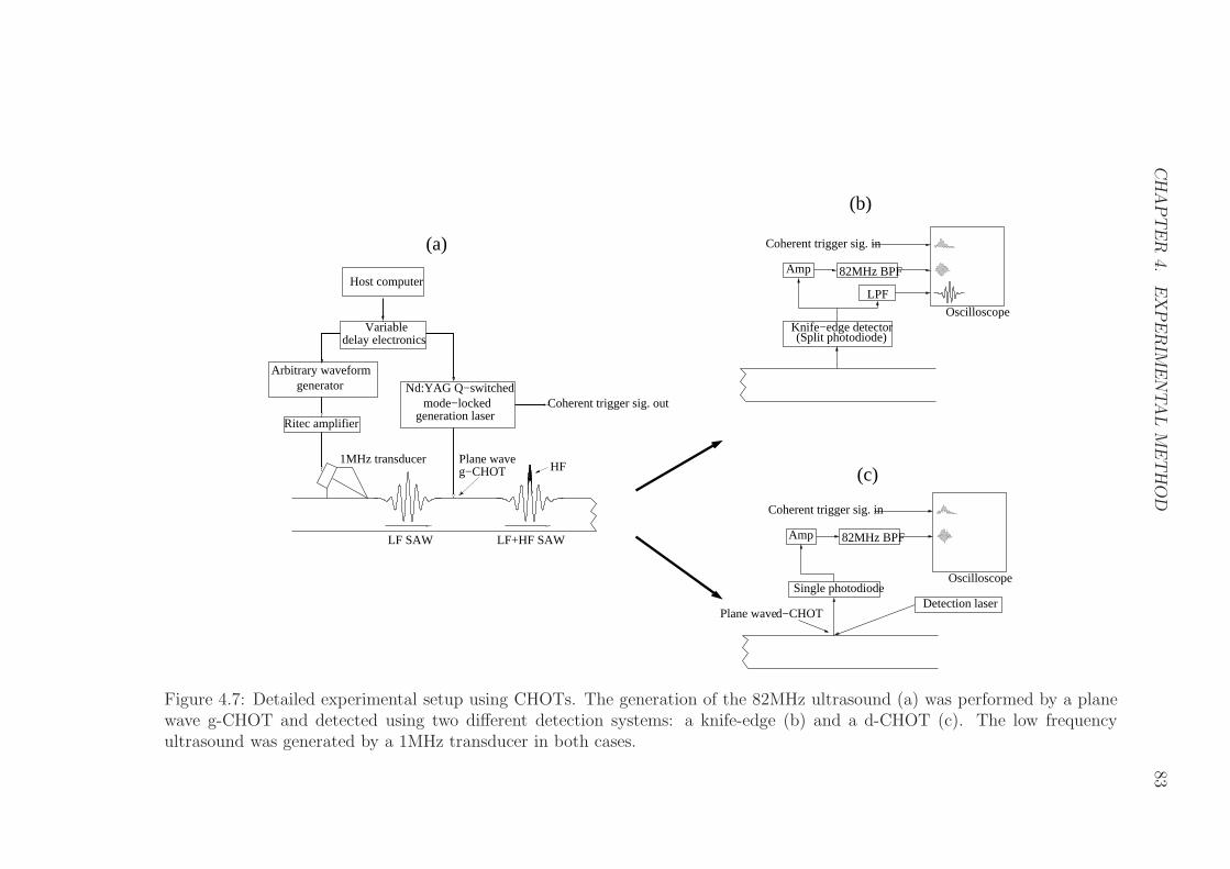
CH
AP
TE
R4.
EX
PE
RIM
EN
TA
LM
ET
HO
D83
1MHz transducer
Host computer
82MHz BPFAmp
82MHz BPFAmp
LPF
Oscilloscope
Detection laserd−CHOT
(a)
(c)
(b)
Coherent trigger sig. out
LF SAW LF+HF SAW
Oscilloscope
g−CHOT
Nd:YAG Q−switchedmode−locked
generation laser
Coherent trigger sig. in
Coherent trigger sig. in
Plane wave
Plane wave
Single photodiode
(Split photodiode)
HF
Arbitrary waveformgenerator
Ritec amplifier
Variabledelay electronics
Knife−edge detector
Figure 4.7: Detailed experimental setup using CHOTs. The generation of the 82MHz ultrasound (a) was performed by a planewave g-CHOT and detected using two different detection systems: a knife-edge (b) and a d-CHOT (c). The low frequencyultrasound was generated by a 1MHz transducer in both cases.

CHAPTER 4. EXPERIMENTAL METHOD 84
Plane d−CHOT
1MHz transducerFocused g−CHOTFocused d−CHOT
Plane g−CHOT
disk sample
Al coating
Fused silica
Figure 4.8: A fused silica sample (100mm diameter, 6mm thickness) with severalCHOTs. The CHOTs used for the experiments presented in this work are directlyin front of the transducer.
other.
4.5 The effects of temperature
Changes in laboratory temperature, even by as little as ±1C overwhelmed the
nonlinear measurements. Temperature change affected the experiment in two ways:
1. Ultrasound velocity is dependent on sample temperature [98].
2. The expansion and contraction of equipment caused changes in the geometrical
setup of the apparatus.
To prevent the experimental equipment from overheating, an air conditioning
unit was required in the laboratory that was able to maintain a mean temperature
of ∼25±1C (figure 4.9). The oscillations in the temperature measurements were
caused by the unit switching on and off every 10 minutes.

CHAPTER 4. EXPERIMENTAL METHOD 85
0 5 10 15 20 25 30 35 40 45 5022
23
24
25
26
27
Roo
m te
mpe
ratu
re (
o C)
Time (mins)
Figure 4.9: Measured room temperature. The oscillations in the measurements werecaused by the air conditioning unit regulating the air temperature.
To demonstrate how the changing laboratory temperature affected the results, an
experiment was performed using an aluminium-2024 sample. The experiment had
a 60-minute duration and the phase of the probe SAW was obtained, along with
room temperature (figure 4.9) and sample temperature. The time interval between
measurements was approximately 13.5 seconds as this was the time required for
the oscilloscope to acquire a single measurement. The sample temperature and
measured probe phase are shown in figure 4.10.
A temperature probe was attached to the rear of the sample itself while a second
was located in an arbitrary location in the laboratory to measure the air temperature.
The sample temperature measurements were accurate to within 0.001C, while the
air temperature was measured with a 0.1C accuracy. During this experiment, the
transducer was turned off, so all the phase modulation was the result of changes
in temperature. The probe phase (green line) gradually increased throughout the
experiment because the incident laser radiation caused the local sample temperature
to rise. In order to demonstrate the high correlation between temperature and phase,
the gradient of the phase data was removed (red line). When normalised with the
sample temperature, the correlation becomes obvious. Figure 4.11 shows the actual
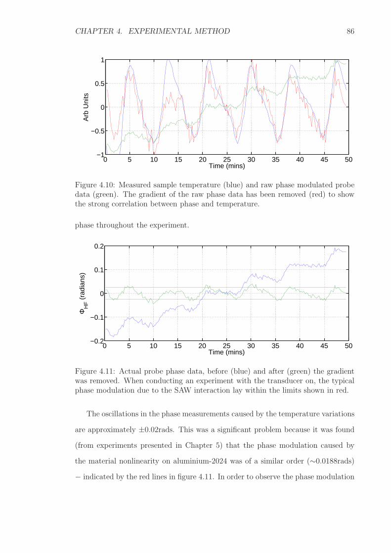
CHAPTER 4. EXPERIMENTAL METHOD 86
0 5 10 15 20 25 30 35 40 45 50−1
−0.5
0
0.5
1
Arb
Uni
ts
Time (mins)
Figure 4.10: Measured sample temperature (blue) and raw phase modulated probedata (green). The gradient of the raw phase data has been removed (red) to showthe strong correlation between phase and temperature.
phase throughout the experiment.
0 5 10 15 20 25 30 35 40 45 50−0.2
−0.1
0
0.1
0.2
ΦH
F (
radi
ans)
Time (mins)
Figure 4.11: Actual probe phase data, before (blue) and after (green) the gradientwas removed. When conducting an experiment with the transducer on, the typicalphase modulation due to the SAW interaction lay within the limits shown in red.
The oscillations in the phase measurements caused by the temperature variations
are approximately ±0.02rads. This was a significant problem because it was found
(from experiments presented in Chapter 5) that the phase modulation caused by
the material nonlinearity on aluminium-2024 was of a similar order (∼0.0188rads)
− indicated by the red lines in figure 4.11. In order to observe the phase modulation
CHAPTER 4. EXPERIMENTAL METHOD 87
caused by the material nonlinearity, the effect of temperature had to be suppressed.
4.6 Suppressing temperature dependence
To minimise the effect of temperature, several suppression techniques were devel-
oped.
4.6.1 Temperature control system
Without any temperature control, the experimental apparatus was exposed to the
changing laboratory temperature and so the ultrasound velocity was affected by the
expansion and contraction of the experimental equipment. The degree of movement
experienced by each element in the experimental setup depended on the material
type and on its position. For example, elements in close proximity to electronics
or heat extractor fans experienced different degrees of temperature variations (and
at different times) than elements that were positioned directly underneath the air
conditioning unit.
Movement of the SLM head relative to the sample, for example, would cause
the SLM image to move on the surface of the sample, thereby affecting the phase
measurement. It was vital that the experimental apparatus was protected from
ambient temperature variations.
A temperature control system was incorporated into the experiment. This con-
sisted of two temperature controlled enclosures − one placed around the sample,
stages and detector system (figure 4.12) and the other placed around the SLM
(These are referred to as the ‘sample’ and ‘SLM’ enclosures respectively).
The walls and lid of each enclosure were constructed from 30mm thick cavity wall
insulation and the internal temperature was regulated by a 33.4W Peltier effect heat
pump. A proportional-integral-derivative (PID) controller unit (Supercool: PR-59)
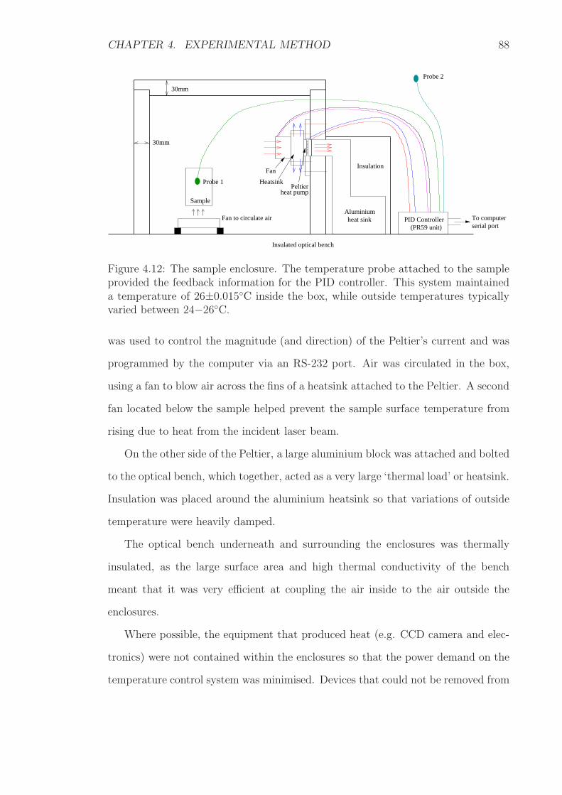
CHAPTER 4. EXPERIMENTAL METHOD 88
Aluminiumheat sink
Probe 2
Probe 1
Sample
Insulated optical bench
Insulation
PID Controller(PR59 unit) serial port
To computer
Fan
PeltierHeatsink
Fan to circulate air
heat pump
30mm
30mm
Figure 4.12: The sample enclosure. The temperature probe attached to the sampleprovided the feedback information for the PID controller. This system maintaineda temperature of 26±0.015C inside the box, while outside temperatures typicallyvaried between 24−26C.
was used to control the magnitude (and direction) of the Peltier’s current and was
programmed by the computer via an RS-232 port. Air was circulated in the box,
using a fan to blow air across the fins of a heatsink attached to the Peltier. A second
fan located below the sample helped prevent the sample surface temperature from
rising due to heat from the incident laser beam.
On the other side of the Peltier, a large aluminium block was attached and bolted
to the optical bench, which together, acted as a very large ‘thermal load’ or heatsink.
Insulation was placed around the aluminium heatsink so that variations of outside
temperature were heavily damped.
The optical bench underneath and surrounding the enclosures was thermally
insulated, as the large surface area and high thermal conductivity of the bench
meant that it was very efficient at coupling the air inside to the air outside the
enclosures.
Where possible, the equipment that produced heat (e.g. CCD camera and elec-
tronics) were not contained within the enclosures so that the power demand on the
temperature control system was minimised. Devices that could not be removed from
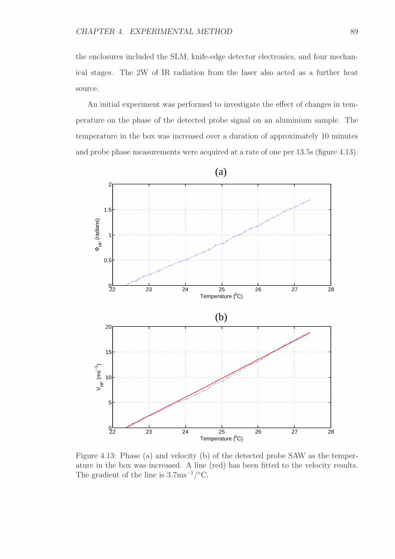
CHAPTER 4. EXPERIMENTAL METHOD 89
the enclosures included the SLM, knife-edge detector electronics, and four mechan-
ical stages. The 2W of IR radiation from the laser also acted as a further heat
source.
An initial experiment was performed to investigate the effect of changes in tem-
perature on the phase of the detected probe signal on an aluminium sample. The
temperature in the box was increased over a duration of approximately 10 minutes
and probe phase measurements were acquired at a rate of one per 13.5s (figure 4.13).
22 23 24 25 26 27 280
5
10
15
20
Temperature (oC)
VH
P (
ms−1
)
22 23 24 25 26 27 280
0.5
1
1.5
2
Temperature (oC)
ΦH
F (
radi
ans)
(a)
(b)
Figure 4.13: Phase (a) and velocity (b) of the detected probe SAW as the temper-ature in the box was increased. A line (red) has been fitted to the velocity results.The gradient of the line is 3.7ms−1/C.
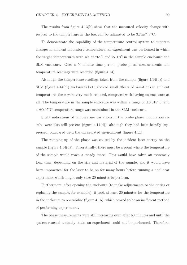
CHAPTER 4. EXPERIMENTAL METHOD 90
The results from figure 4.13(b) show that the measured velocity change with
respect to the temperature in the box can be estimated to be 3.7ms−1/C.
To demonstrate the capability of the temperature control system to suppress
changes in ambient laboratory temperature, an experiment was performed in which
the target temperatures were set at 26C and 27.1C in the sample enclosure and
SLM enclosure. Over a 50-minute time period, probe phase measurements and
temperature readings were recorded (figure 4.14).
Although the temperature readings taken from the sample (figure 4.14(b)) and
SLM (figure 4.14(c)) enclosures both showed small effects of variations in ambient
temperature, these were very much reduced, compared with having no enclosure at
all. The temperature in the sample enclosure was within a range of ±0.015C, and
a ±0.05C temperature range was maintained in the SLM enclosure.
Slight indications of temperature variations in the probe phase modulation re-
sults were also still present (figure 4.14(d)), although they had been heavily sup-
pressed, compared with the unregulated environment (figure 4.11).
The ramping up of the phase was caused by the incident laser energy on the
sample (figure 4.14(d)). Theoretically, there must be a point where the temperature
of the sample would reach a steady state. This would have taken an extremely
long time, depending on the size and material of the sample, and it would have
been impractical for the laser to be on for many hours before running a nonlinear
experiment which might only take 20 minutes to perform.
Furthermore, after opening the enclosure (to make adjustments to the optics or
replacing the sample, for example), it took at least 20 minutes for the temperature
in the enclosure to re-stabilise (figure 4.15), which proved to be an inefficient method
of performing experiments.
The phase measurements were still increasing even after 60 minutes and until the
system reached a steady state, an experiment could not be performed. Therefore,
CHAPTER 4. EXPERIMENTAL METHOD 91
0 5 10 15 20 25 30 35 40 45 5025.98
25.99
26
26.01
26.02
Sam
ple
tem
pera
ture
(o C
)
Time (mins)
0 5 10 15 20 25 30 35 40 45 50−0.05−0.04−0.03−0.02−0.01
00.010.020.030.040.05
ΦH
F (
radi
ans)
Time (mins)
0 5 10 15 20 25 30 35 40 45 5022
23
24
25
26
27
Roo
m te
mpe
ratu
re (
o C)
Time (mins)
0 5 10 15 20 25 30 35 40 45 5026.9
27
27.1
27.2
27.3
SLM
tem
pera
ture
(o C
)
Time (mins)
(b)
(c)
(d)
(a)
Figure 4.14: Measured laboratory (a), sample enclosure (b) and SLM enclosure (c)temperatures. The probe phase measurements are shown in (d) and the red linesindicate the limits of the modulation caused by material nonlinearity.
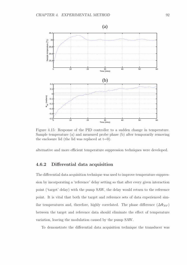
CHAPTER 4. EXPERIMENTAL METHOD 92
0 10 20 30 40 50 60
25.4
25.6
25.8
26
26.2
Sam
ple
tem
pera
ture
(o C
)
Time (mins)
0 10 20 30 40 50 60−0.5
−0.4
−0.3
−0.2
−0.1
0
0.1
0.2
ΦH
F (
radi
ans)
Time (mins)
(a)
(b)
Figure 4.15: Response of the PID controller to a sudden change in temperature.Sample temperature (a) and measured probe phase (b) after temporarily removingthe enclosure lid (the lid was replaced at t=0).
alternative and more efficient temperature suppression techniques were developed.
4.6.2 Differential data acquisition
The differential data acquisition technique was used to improve temperature suppres-
sion by incorporating a ‘reference’ delay setting so that after every given interaction
point (‘target’ delay) with the pump SAW, the delay would return to the reference
point. It is vital that both the target and reference sets of data experienced sim-
ilar temperatures and, therefore, highly correlated. The phase difference (∆ΦHF )
between the target and reference data should eliminate the effect of temperature
variation, leaving the modulation caused by the pump SAW.
To demonstrate the differential data acquisition technique the transducer was

CHAPTER 4. EXPERIMENTAL METHOD 93
not turned on but the temperature and phase measurements were recorded over a
period of 50 minutes (figure 4.16).
The laboratory temperature variations (figure 4.16(a)) were still observed in the
reference and target measurements (figure 4.16(b)). However, the phase difference
between the data sets (figure 4.16(c)) showed only slight variations, which were heav-
ily damped. Furthermore, the overall phase difference remained stable throughout
the course of the 45-minute experiment and showed no evidence of ramping-up (fig-
ure 4.16(c)).
Slight variations still exist because it is not possible to acquire the target and
reference data simultaneously. Therefore, there is a temperature difference between
taking the reference and target data. To lessen the effect of temperature further,
using this method, the time difference between obtaining the reference and target
data would have to be reduced. Although this could be achieved by reducing the
number of averages/measurement, the subsequent loss of SNR would be undesirable.
Therefore, an alternative method was developed.
4.6.3 Interlacing differential data acquisition
With the interlacing differential data acquisition method, the reference and target
data are acquired simultaneously (figure 4.17). This method interlaces the reference
and target data by switching between them at a relatively high speed (≥10Hz).
Thus, as the average temperature at the times of taking the reference and target
data is highly correlated, the mean temperature difference between measurements
is minimised. Two channels of the oscilloscope were used simultaneously − one for
the reference data and the other for the target data.
Two switches (S1 and S2), were operated by the same 5V square wave. An
inverter (I) placed before one of the switches meant that only one of these switches
could be on at a single moment in time. The switching waveform came directly from

CHAPTER 4. EXPERIMENTAL METHOD 94
0 5 10 15 20 25 30 35 40 45 501.55
1.57
1.59
1.61
1.63
1.65
ΦH
F (
radi
ans)
Time (mins)
0 5 10 15 20 25 30 35 40 45 50−0.05−0.04−0.03−0.02−0.01
00.010.020.030.040.05
∆ΦH
F (
radi
ans)
Time (mins)
0 5 10 15 20 25 30 35 40 45 5021
21.5
22
22.5
23T
empe
ratu
re (o C
)
Time (mins)
(b)
(c)
(a)
Figure 4.16: Laboratory temperature (a), phase measurements at the target (blue)and reference (green) delays (b) and phase difference (∆ΦHF ) is shown in (c).
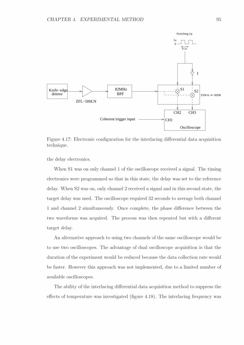
CHAPTER 4. EXPERIMENTAL METHOD 95
5v0
0.1s
Oscilloscope
CH1
detetorKnife−edge
ZFL−500LN
82MHzBPF
CH2 CH3
S1 S2
I
Switching i/p
ZSWA−4−30DR
Coherent trigger input
Figure 4.17: Electronic configuration for the interlacing differential data acquisitiontechnique.
the delay electronics.
When S1 was on only channel 1 of the oscilloscope received a signal. The timing
electronics were programmed so that in this state, the delay was set to the reference
delay. When S2 was on, only channel 2 received a signal and in this second state, the
target delay was used. The oscilloscope required 32 seconds to average both channel
1 and channel 2 simultaneously. Once complete, the phase difference between the
two waveforms was acquired. The process was then repeated but with a different
target delay.
An alternative approach to using two channels of the same oscilloscope would be
to use two oscilloscopes. The advantage of dual oscilloscope acquisition is that the
duration of the experiment would be reduced because the data collection rate would
be faster. However this approach was not implemented, due to a limited number of
available oscilloscopes.
The ability of the interlacing differential data acquisition method to suppress the
effects of temperature was investigated (figure 4.18). The interlacing frequency was
CHAPTER 4. EXPERIMENTAL METHOD 96
50Hz and the transducer remained off for the duration of the experiment.
Over the 25 minutes the phase difference remained stable and within limits in
which nonlinearity could be measured (shown in red, figure 4.18(c)).
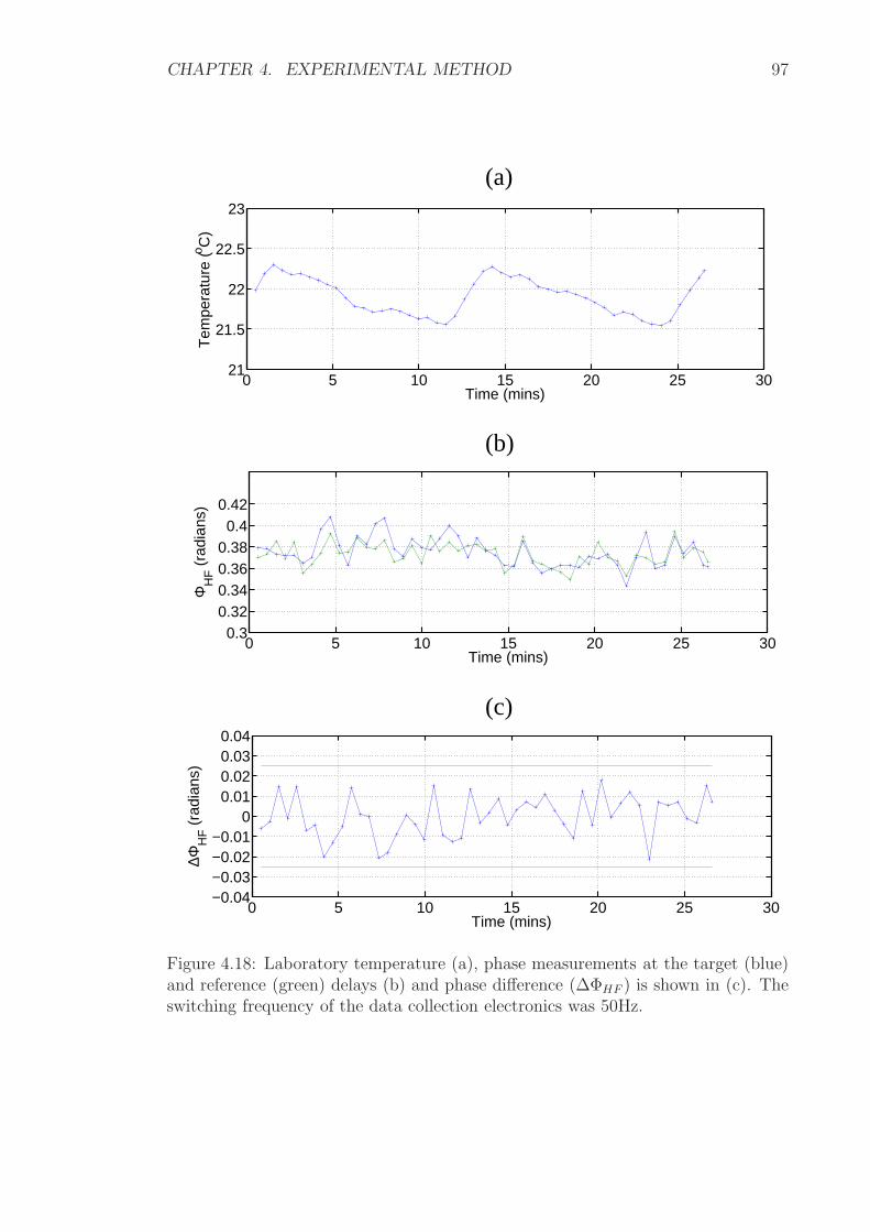
CHAPTER 4. EXPERIMENTAL METHOD 97
0 5 10 15 20 25 3021
21.5
22
22.5
23T
empe
ratu
re (o C
)
Time (mins)
0 5 10 15 20 25 300.3
0.320.340.360.380.4
0.42
ΦH
F (
radi
ans)
Time (mins)
0 5 10 15 20 25 30−0.04−0.03−0.02−0.01
00.010.020.030.04
∆ΦH
F (
radi
ans)
Time (mins)
(b)
(a)
(c)
Figure 4.18: Laboratory temperature (a), phase measurements at the target (blue)and reference (green) delays (b) and phase difference (∆ΦHF ) is shown in (c). Theswitching frequency of the data collection electronics was 50Hz.
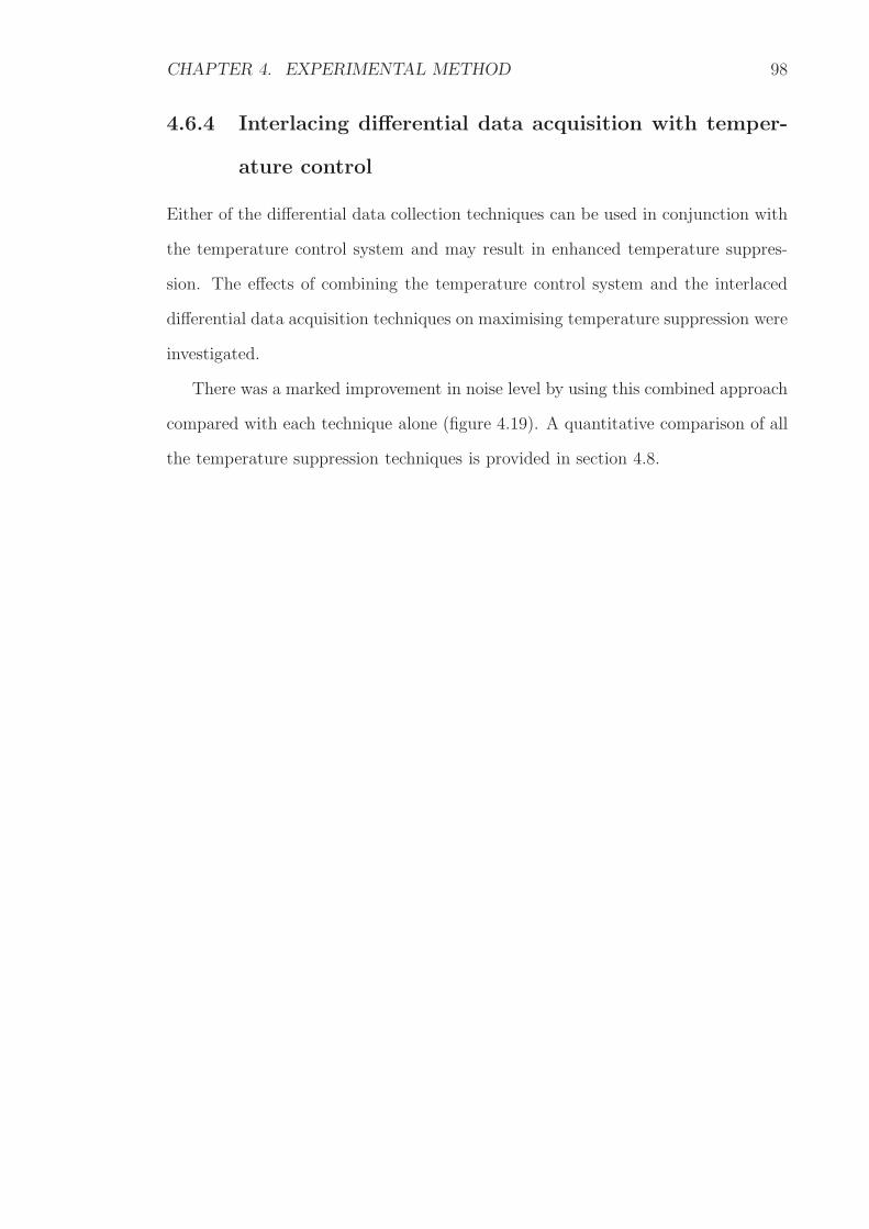
CHAPTER 4. EXPERIMENTAL METHOD 98
4.6.4 Interlacing differential data acquisition with temper-
ature control
Either of the differential data collection techniques can be used in conjunction with
the temperature control system and may result in enhanced temperature suppres-
sion. The effects of combining the temperature control system and the interlaced
differential data acquisition techniques on maximising temperature suppression were
investigated.
There was a marked improvement in noise level by using this combined approach
compared with each technique alone (figure 4.19). A quantitative comparison of all
the temperature suppression techniques is provided in section 4.8.
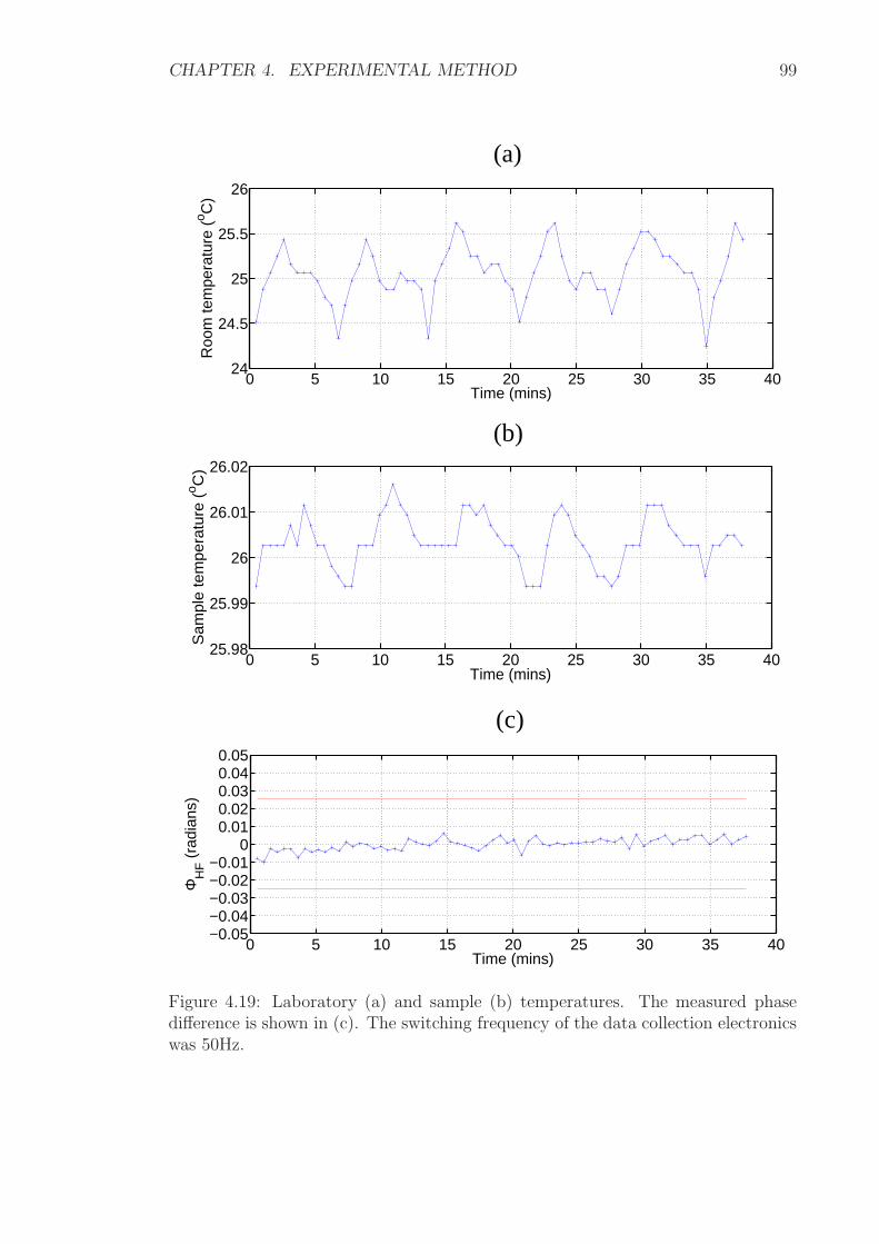
CHAPTER 4. EXPERIMENTAL METHOD 99
0 5 10 15 20 25 30 35 4024
24.5
25
25.5
26R
oom
tem
pera
ture
(o C
)
Time (mins)
0 5 10 15 20 25 30 35 40−0.05−0.04−0.03−0.02−0.01
00.010.020.030.040.05
ΦH
F (
radi
ans)
Time (mins)
0 5 10 15 20 25 30 35 4025.98
25.99
26
26.01
26.02
Sam
ple
tem
pera
ture
(o C
)
Time (mins)
(a)
(c)
(b)
Figure 4.19: Laboratory (a) and sample (b) temperatures. The measured phasedifference is shown in (c). The switching frequency of the data collection electronicswas 50Hz.
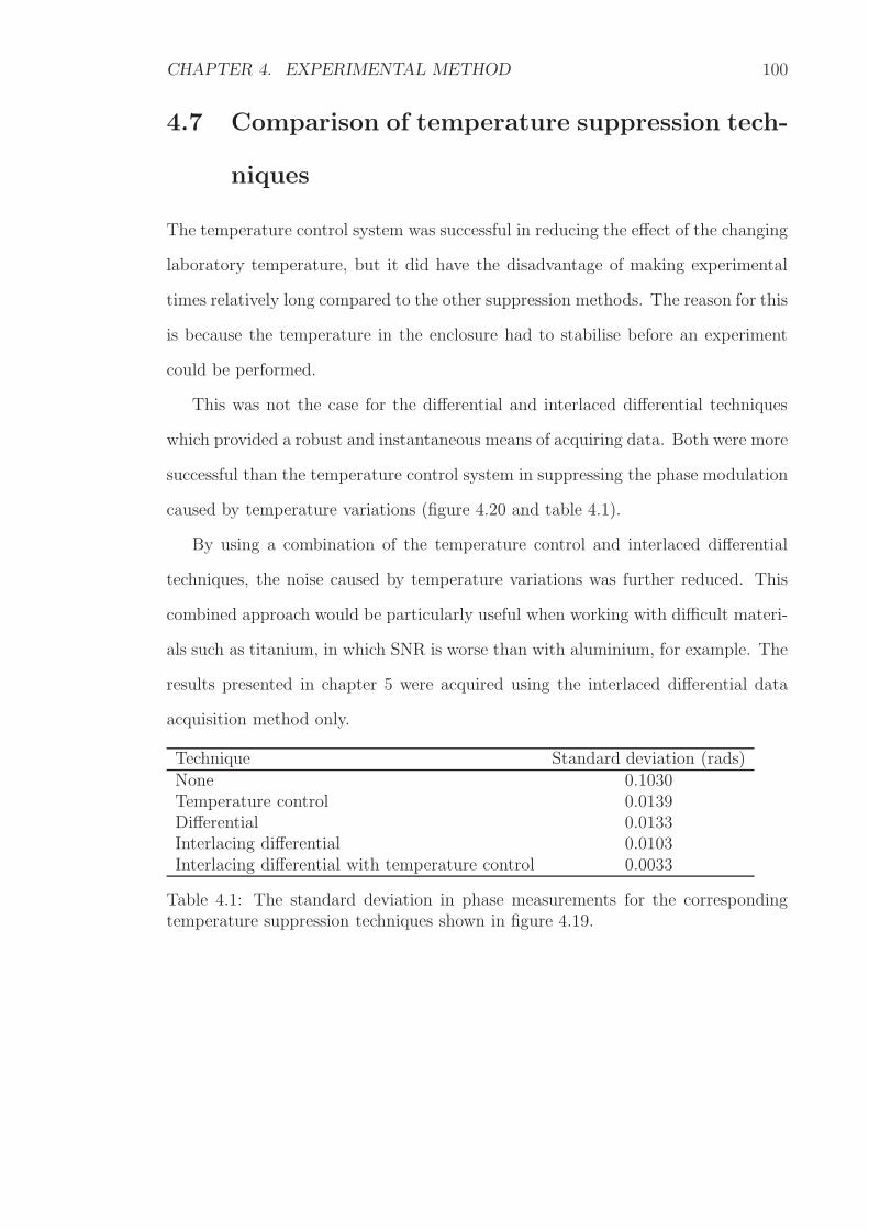
CHAPTER 4. EXPERIMENTAL METHOD 100
4.7 Comparison of temperature suppression tech-
niques
The temperature control system was successful in reducing the effect of the changing
laboratory temperature, but it did have the disadvantage of making experimental
times relatively long compared to the other suppression methods. The reason for this
is because the temperature in the enclosure had to stabilise before an experiment
could be performed.
This was not the case for the differential and interlaced differential techniques
which provided a robust and instantaneous means of acquiring data. Both were more
successful than the temperature control system in suppressing the phase modulation
caused by temperature variations (figure 4.20 and table 4.1).
By using a combination of the temperature control and interlaced differential
techniques, the noise caused by temperature variations was further reduced. This
combined approach would be particularly useful when working with difficult materi-
als such as titanium, in which SNR is worse than with aluminium, for example. The
results presented in chapter 5 were acquired using the interlaced differential data
acquisition method only.
Technique Standard deviation (rads)None 0.1030Temperature control 0.0139Differential 0.0133Interlacing differential 0.0103Interlacing differential with temperature control 0.0033
Table 4.1: The standard deviation in phase measurements for the correspondingtemperature suppression techniques shown in figure 4.19.

CHAPTER 4. EXPERIMENTAL METHOD 101
0 5 10 15 20 25 30 35−0.05
−0.03
−0.01
0.01
0.03
0.05
0 5 10 15 20 25 30 35−0.05
−0.03
−0.01
0.01
0.03
0.05
0 5 10 15 20 25 30 35−0.05
−0.03
−0.01
0.01
0.03
0.05
0 5 10 15 20 25 30 35−0.05
−0.03
−0.01
0.01
0.03
0.05
0 5 10 15 20 25 30 35−0.05
−0.03
−0.01
0.01
0.03
0.05
φ HF
(rad
ians
)
(a)
(b)
(c)
(d)
(e)
0 5 10 15 20 25 30 35
0 5 10 15 20 25 30 35
0 5 10 15 20 25 30 35
0 5 10 15 20 25 30 35
Time (mins)
5 10 15 20 25 30 350
0.030.01
0.05
0.03
−0.01−0.03
0.01
0.05
0.03
−0.010.01
0.05
0.03
−0.010.01
0.05
0.03
−0.010.01
0.05
−0.01−0.03−0.05
−0.05
−0.05−0.03
−0.03−0.05
−0.05−0.03
(a)
(b)
(c)
(d)
(e)
Figure 4.20: Measured phase difference from each of the temperature suppressiontechniques. No control (a), temperature control system (b), differential data acquisi-tion (c), interlaced differential data acquisition (d) and a combination of temperaturecontrol and interlaced data acquisition (e).
4.8 Summary
In order to perform nonlinear experiments, a number of modifications had to be
made to the OSAM instrument, which includes the integration of: the pump SAW
generation system, the timing control electronics and a robust method of suppressing
the effects of temperature on the measurements.
The pump SAW system consisted of a transducer bonded to the sample and the
timing control electronics controlled the interaction point of the pump and probe
SAWs to within an 8ns accuracy. Changes in ambient laboratory temperature had a
large impact on the probe phase. Room temperature changes of ±1C were causing
phase changes that were of the same order as the nonlinear measurements. A num-

CHAPTER 4. EXPERIMENTAL METHOD 102
ber of temperature suppression techniques were developed. The most appropriate
technique was the interlaced differential data acquisition method, because it pro-
vided adequate suppression of the temperature effect and was immediately effective
− unlike the temperature control system.
CHOTs provide an alternative method of generating and detecting ultrasound
and have the fundamental advantage over the SLM/ knife-edge detector configura-
tion in that they drastically simplify the optical setup, as well as offering a robust
and compact method of performing the nonlinear experiment.

Chapter 5
Experimental Results
5.1 Introduction
Fused silica and aluminium are reported to have a relatively high nonlinearity prop-
erty compared with titanium for example [4]. Therefore these materials are suitable
for the initial development of a nonlinear experiment.
The purpose of the experiment, described in section 5.3, was to verify that the
observed measurements were caused by the material nonlinearity and not caused by
an artefact of the experiment. The effect of using different pump SAW amplitudes
on the experiment is described in section 5.4. Experiments using several pump:probe
frequency ratios are also demonstrated in this chapter. In section 5.5, pump SAWs at
0.5MHz, 1MHz and 2MHz were mixed with an 82MHz probe pulse and the measured
phase modulation in the probe pulse was compared. In addition, to demonstrate that
the nonlinear experiment can be performed using different probe SAW frequencies,
three experiments were conducted and discussed in section 5.6. Here, a 1MHz
pump SAW interacted with an 82MHz, 164MHz and 246MHz probe SAW and the
results were compared. In section 5.7, the nonlinear response of aluminium-2024,
aluminium-6061 and fused silica were compared.
103
CHAPTER 5. EXPERIMENTAL RESULTS 104
5.2 Extracting the phase
The raw data consists of a number of detected probe SAW signals that have in-
teracted with various points (due to the delay settings) of the pump’s wave packet
and have therefore experienced some degree of phase modulation. Typically, 20000
points were used for each trace, providing a time resolution of 0.1ns/point, which was
an adequate resolution to extract the phase of the probe signal. The phase was ex-
tracted by taking the fast Fourier transform (FFT) of the received signal and within
the frequency spectrum, the point that corresponded to the 82MHz component was
located. The phase at this point was then converted to a velocity.
Results herein are presented in terms of velocity-stress graphs and the gradient of
the velocity-stress data provides a measure of the material nonlinearity. The gradient
was calculated using the method of least-squares. The error in the gradients was
also established, based on the statistical spread of the data.
5.3 Validation of nonlinear measurement − the
‘anti-propagating’ test
It was important to confirm that the phase changes being measured were purely
caused by the pump-probe SAW interaction and not by an experimental artefact,
such as signal crosstalk or electronic noise. The ‘anti-propagating’ test was per-
formed to rule out any concern of whether the pump SAW signal had not been
completely filtered out by the 82MHz bandpass filter and, therefore, was influencing
the probe signal phase measurements.
When the pump and probe SAWs co-propagated, the probe pulse interacted with
a single point of the pump SAW and experienced a constant stressed state. When
the two SAWs propagated in opposite directions, they did so over different parts
of the sample surface, in which case the probe SAW did not experience a constant
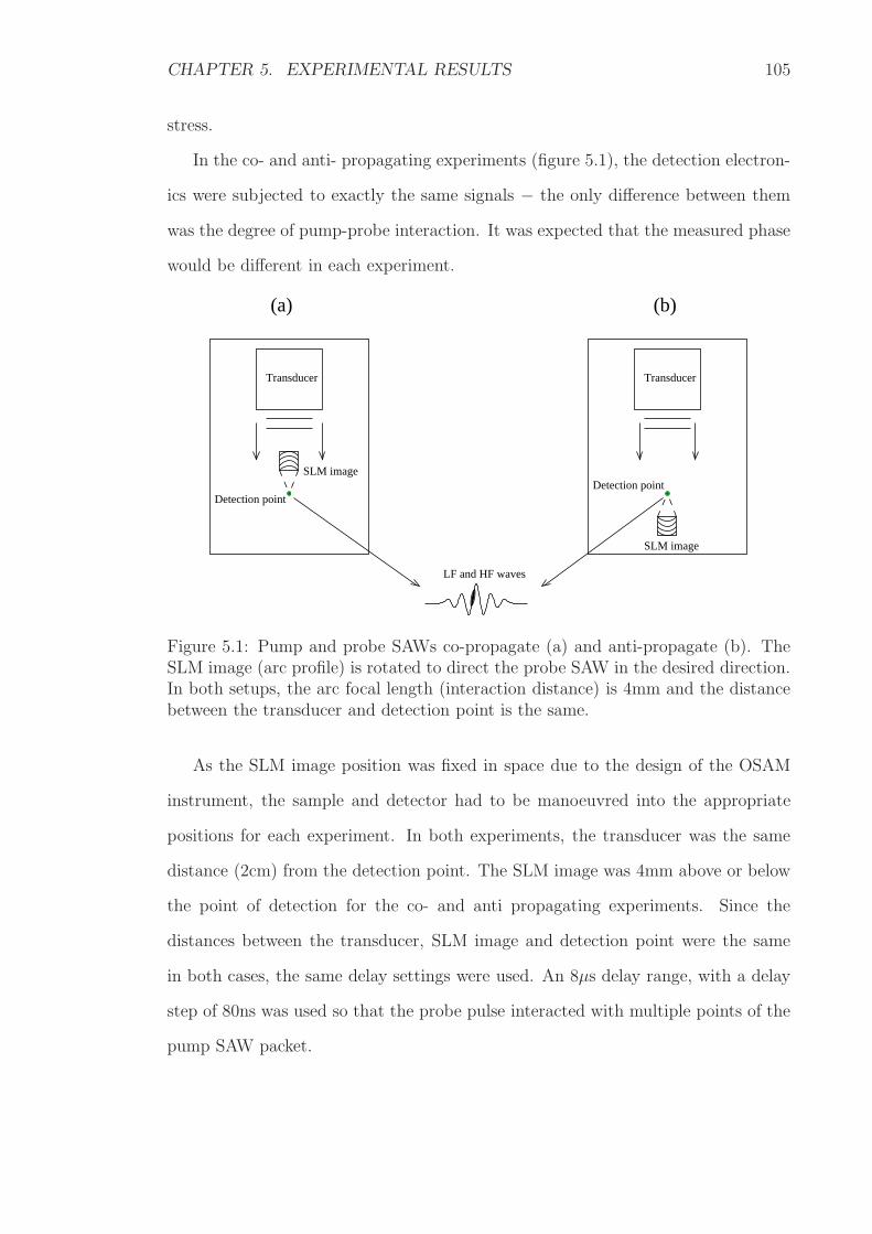
CHAPTER 5. EXPERIMENTAL RESULTS 105
stress.
In the co- and anti- propagating experiments (figure 5.1), the detection electron-
ics were subjected to exactly the same signals − the only difference between them
was the degree of pump-probe interaction. It was expected that the measured phase
would be different in each experiment.
Transducer
SLM image
Detection point
LF and HF waves
(b)(a)
SLM image
Transducer
Detection point
Figure 5.1: Pump and probe SAWs co-propagate (a) and anti-propagate (b). TheSLM image (arc profile) is rotated to direct the probe SAW in the desired direction.In both setups, the arc focal length (interaction distance) is 4mm and the distancebetween the transducer and detection point is the same.
As the SLM image position was fixed in space due to the design of the OSAM
instrument, the sample and detector had to be manoeuvred into the appropriate
positions for each experiment. In both experiments, the transducer was the same
distance (2cm) from the detection point. The SLM image was 4mm above or below
the point of detection for the co- and anti propagating experiments. Since the
distances between the transducer, SLM image and detection point were the same
in both cases, the same delay settings were used. An 8µs delay range, with a delay
step of 80ns was used so that the probe pulse interacted with multiple points of the
pump SAW packet.
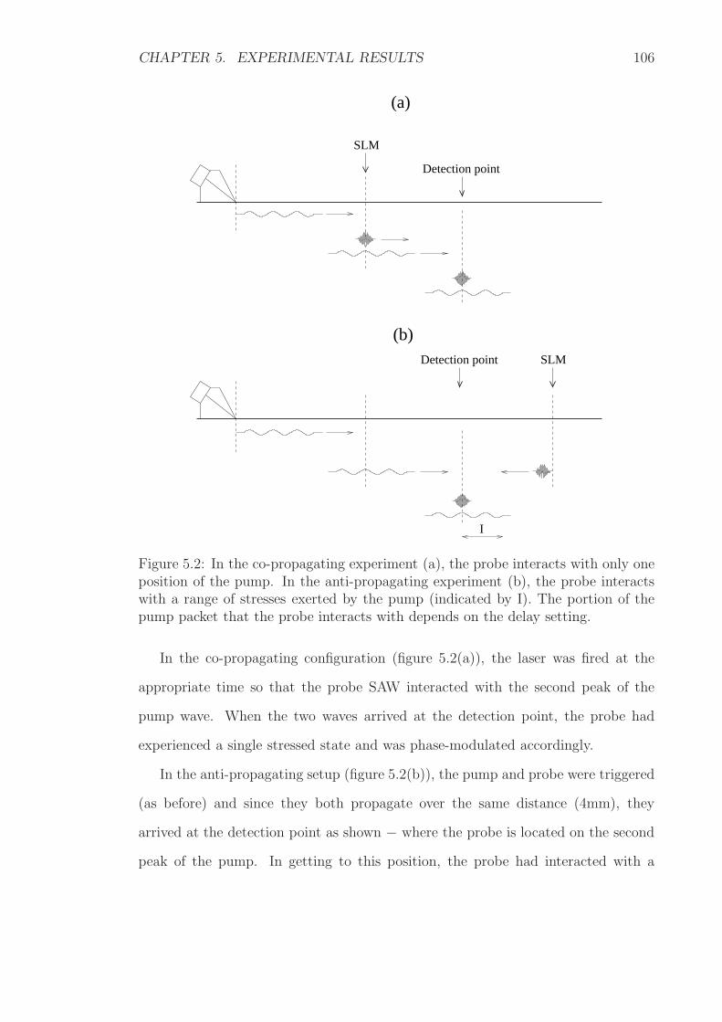
CHAPTER 5. EXPERIMENTAL RESULTS 106
Detection point SLM
SLM
I
(b)
(a)
Detection point
Figure 5.2: In the co-propagating experiment (a), the probe interacts with only oneposition of the pump. In the anti-propagating experiment (b), the probe interactswith a range of stresses exerted by the pump (indicated by I). The portion of thepump packet that the probe interacts with depends on the delay setting.
In the co-propagating configuration (figure 5.2(a)), the laser was fired at the
appropriate time so that the probe SAW interacted with the second peak of the
pump wave. When the two waves arrived at the detection point, the probe had
experienced a single stressed state and was phase-modulated accordingly.
In the anti-propagating setup (figure 5.2(b)), the pump and probe were triggered
(as before) and since they both propagate over the same distance (4mm), they
arrived at the detection point as shown − where the probe is located on the second
peak of the pump. In getting to this position, the probe had interacted with a

CHAPTER 5. EXPERIMENTAL RESULTS 107
portion of the pump wave (indicated by I). This means the probe had experienced
all the stresses imposed by this portion of the pump wave. The measured phase of
the probe was, therefore, an averaged phase change caused by all of these imposed
stresses (figure 5.3).
Using the experimental setup in section 4.3, different electronic channels were
used for detecting the pump and probe signals. Consequently, the two signals experi-
enced different delays. This meant that it was not possible to accurately determine
the precise location of the probe SAW relative to the pump. Therefore, an arbi-
trary phase was applied to the results in figure 5.3 so that they coincide with their
respective interaction points on the pump SAW packet.
The co-propagating experiment showed a clear correlation between the interac-
tion points and the phase-modulated measurements. In the anti-propagating exper-
iment, the phase modulation appeared to be barely above the noise level. There
is clearly a difference between the results from the two setups, confirming that the
phase-modulation experienced by the probe SAW is caused by the material nonlin-
earity and not by an experimental artefact.
5.4 Changing the pump SAW amplitude
To observe the pump-probe interaction, the approach used in section 5.3 altered
the triggering delay between the two SAWs so that the probe experienced multiple
stress states imposed on the sample by the pump SAW. In this section, the stress
imposed by the transducer on the sample was changed by controlling the amplitude
of the pump wave and the corresponding probe phase modulation was measured.
Only two delay settings were required − a reference and a target delay − and using
the interlaced differential data acquisition method, the delay alternated between the
two settings at a rate of 50Hz.
The most appropriate reference and target delay settings for this experiment

CHAPTER 5. EXPERIMENTAL RESULTS 108
(a)
1 1.5 2 2.5 3 3.5 4 4.5 5 5.5 6−0.05
−0.04
−0.03
−0.02
−0.01
0
0.01
0.02
0.03
0.04
0.05
∆ΦH
F (
radi
ans)
ΦLF
(µs)
(b)
1 1.5 2 2.5 3 3.5 4 4.5 5 5.5 6−0.05
−0.04
−0.03
−0.02
−0.01
0
0.01
0.02
0.03
0.04
0.05
∆ΦH
F (
radi
ans)
ΦLF
(µs)
Figure 5.3: Probe phase modulation (green) when interacting with the pump SAWpacket (blue) as the two SAWs are co-propagating (a) and anti-propagating (b).
CHAPTER 5. EXPERIMENTAL RESULTS 109
were those that corresponded to the maximum and minimum stress levels imposed
by the pump wave. However, since the detected pump and probe signals had different
electronic paths, a procedure was developed to overcome the difficulty of accurately
establishing which delay values corresponded to these interaction positions.
5.4.1 Selecting appropriate delay settings
The points of maximum and minimum stress are at the peak and trough of the
pump wave and have half a cycle difference, in terms of time. The time difference
between the reference and target delays was fixed at 0.5µs (since a 1MHz transducer
was used) and both delays were incremented so that the probe pulse interacted with
the pump wave. The phase modulation experienced at each of the reference and
target delays is shown in figure 5.4.
The two delays that provide the greatest contrast in terms of phase modulation
are measurements 25 and 31 (REF and TAR, respectively), and are the most ap-
propriate ones to use. It would be unwise to use the delay settings at measurements
28 and 34 because this would result in little or no stress contrast, regardless of
the pump SAW amplitude, thereby making the experiment unsuccessful. A trace
was obtained to show the probe SAW location relative to the pump SAW at delay
measurements 25 and 31 (figure 5.5).
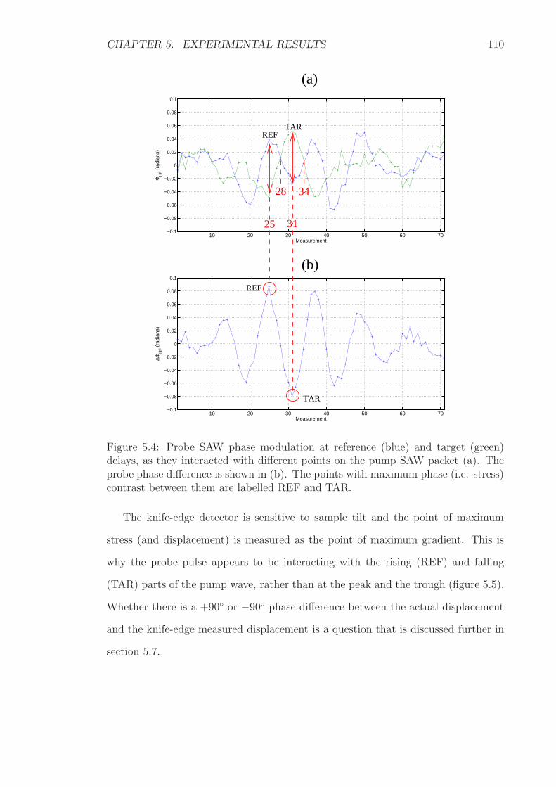
CHAPTER 5. EXPERIMENTAL RESULTS 110
10 20 30 40 50 60 70−0.1
−0.08
−0.06
−0.04
−0.02
0
0.02
0.04
0.06
0.08
0.1
Measurement
ΦH
F (
radi
ans)
10 20 30 40 50 60 70−0.1
−0.08
−0.06
−0.04
−0.02
0
0.02
0.04
0.06
0.08
0.1
Measurement
∆ΦH
F (
radi
ans)
REFTAR
REF
TAR
3125
3428
(a)
(b)
Figure 5.4: Probe SAW phase modulation at reference (blue) and target (green)delays, as they interacted with different points on the pump SAW packet (a). Theprobe phase difference is shown in (b). The points with maximum phase (i.e. stress)contrast between them are labelled REF and TAR.
The knife-edge detector is sensitive to sample tilt and the point of maximum
stress (and displacement) is measured as the point of maximum gradient. This is
why the probe pulse appears to be interacting with the rising (REF) and falling
(TAR) parts of the pump wave, rather than at the peak and the trough (figure 5.5).
Whether there is a +90 or −90 phase difference between the actual displacement
and the knife-edge measured displacement is a question that is discussed further in
section 5.7.
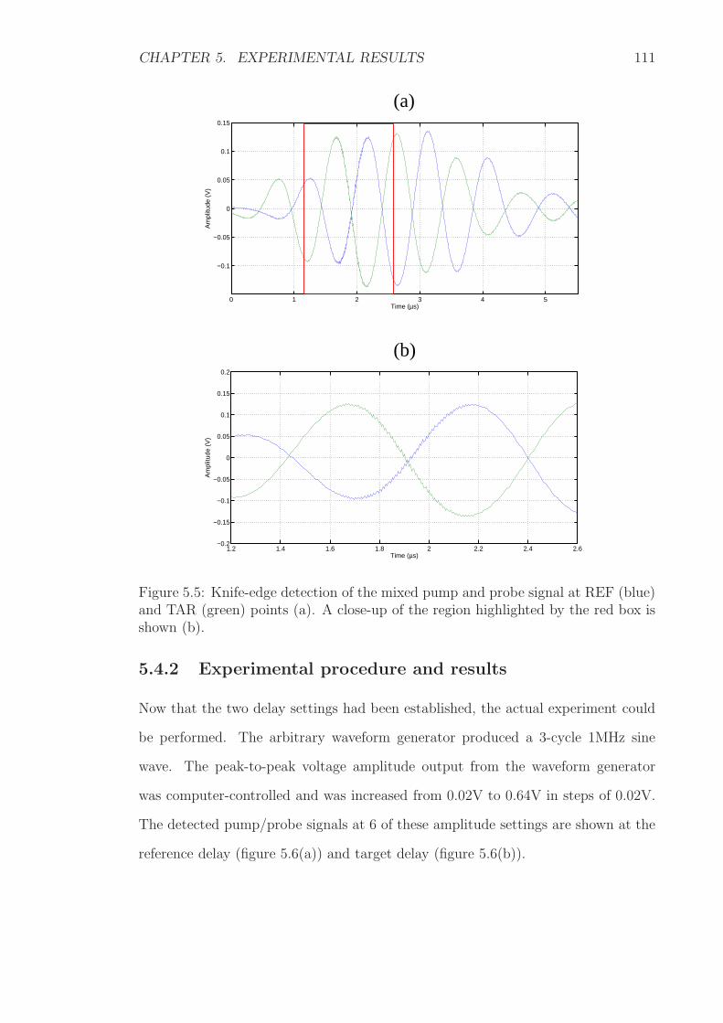
CHAPTER 5. EXPERIMENTAL RESULTS 111
0 1 2 3 4 5
−0.1
−0.05
0
0.05
0.1
0.15
Time (µs)
Am
plitu
de (
V)
1.2 1.4 1.6 1.8 2 2.2 2.4 2.6−0.2
−0.15
−0.1
−0.05
0
0.05
0.1
0.15
0.2
Time (µs)
Am
plitu
de (
V)
(b)
(a)
Figure 5.5: Knife-edge detection of the mixed pump and probe signal at REF (blue)and TAR (green) points (a). A close-up of the region highlighted by the red box isshown (b).
5.4.2 Experimental procedure and results
Now that the two delay settings had been established, the actual experiment could
be performed. The arbitrary waveform generator produced a 3-cycle 1MHz sine
wave. The peak-to-peak voltage amplitude output from the waveform generator
was computer-controlled and was increased from 0.02V to 0.64V in steps of 0.02V.
The detected pump/probe signals at 6 of these amplitude settings are shown at the
reference delay (figure 5.6(a)) and target delay (figure 5.6(b)).
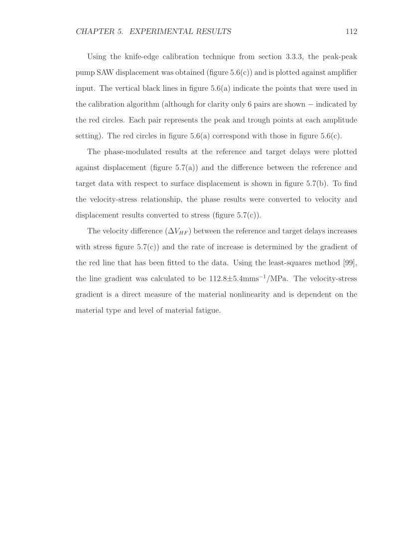
CHAPTER 5. EXPERIMENTAL RESULTS 112
Using the knife-edge calibration technique from section 3.3.3, the peak-peak
pump SAW displacement was obtained (figure 5.6(c)) and is plotted against amplifier
input. The vertical black lines in figure 5.6(a) indicate the points that were used in
the calibration algorithm (although for clarity only 6 pairs are shown − indicated by
the red circles. Each pair represents the peak and trough points at each amplitude
setting). The red circles in figure 5.6(a) correspond with those in figure 5.6(c).
The phase-modulated results at the reference and target delays were plotted
against displacement (figure 5.7(a)) and the difference between the reference and
target data with respect to surface displacement is shown in figure 5.7(b). To find
the velocity-stress relationship, the phase results were converted to velocity and
displacement results converted to stress (figure 5.7(c)).
The velocity difference (∆VHF ) between the reference and target delays increases
with stress figure 5.7(c)) and the rate of increase is determined by the gradient of
the red line that has been fitted to the data. Using the least-squares method [99],
the line gradient was calculated to be 112.8±5.4mms−1/MPa. The velocity-stress
gradient is a direct measure of the material nonlinearity and is dependent on the
material type and level of material fatigue.

CHAPTER 5. EXPERIMENTAL RESULTS 113
0 0.1 0.2 0.3 0.4 0.5 0.6 0.70
10
20
30
40
50
Pe
ak−
Pe
ak D
isp
lace
me
nt
(nm
)
Amplifier input (Vpp)
0 1 2 3 4 5 6−0.2
−0.15
−0.1
−0.05
0
0.05
0.1
0.15
0.2
Time (µs)
Am
plitu
de (
V)
0 1 2 3 4 5 6−0.2
−0.15
−0.1
−0.05
0
0.05
0.1
0.15
0.2
Time (µs)
Am
plitu
de (
V)
(b)
(a)
(c)
Trough amps
Peak amps
Figure 5.6: Example pump/probe detected signals at various pump amplitude set-tings at the reference (a) and target (b) delay settings. The surface displacementsmeasured at increasing input voltages to the amplifier are shown (c).

CHAPTER 5. EXPERIMENTAL RESULTS 114
0 5 10 15 20 25 30 35 40 45 502.45
2.5
2.55
2.6
2.65
2.7
ΦH
F (
radi
ans)
Peak−Peak Displacement (nm)
0 5 10 15 20 25 30 35 40 45 500
0.02
0.04
0.06
0.08
0.1
∆ΦH
F (
radi
ans
pp)
Peak−Peak Displacement (nm)
0 0.5 1 1.5 2 2.5 3 3.5 4 4.5 50
0.2
0.4
0.6
0.8
∆ V
HF (
ms−
1 pp)
Peak−Peak Stress (MPa)
(a)
(b)
(c)
Figure 5.7: Phase modulation at REF (blue) and TAR (green) interaction pointswith corresponding surface displacement caused by the pump SAW (a). Differentialprobe phase modulation with corresponding surface displacement caused by thepump SAW (b). The corresponding velocity and applied stress is shown in (c).
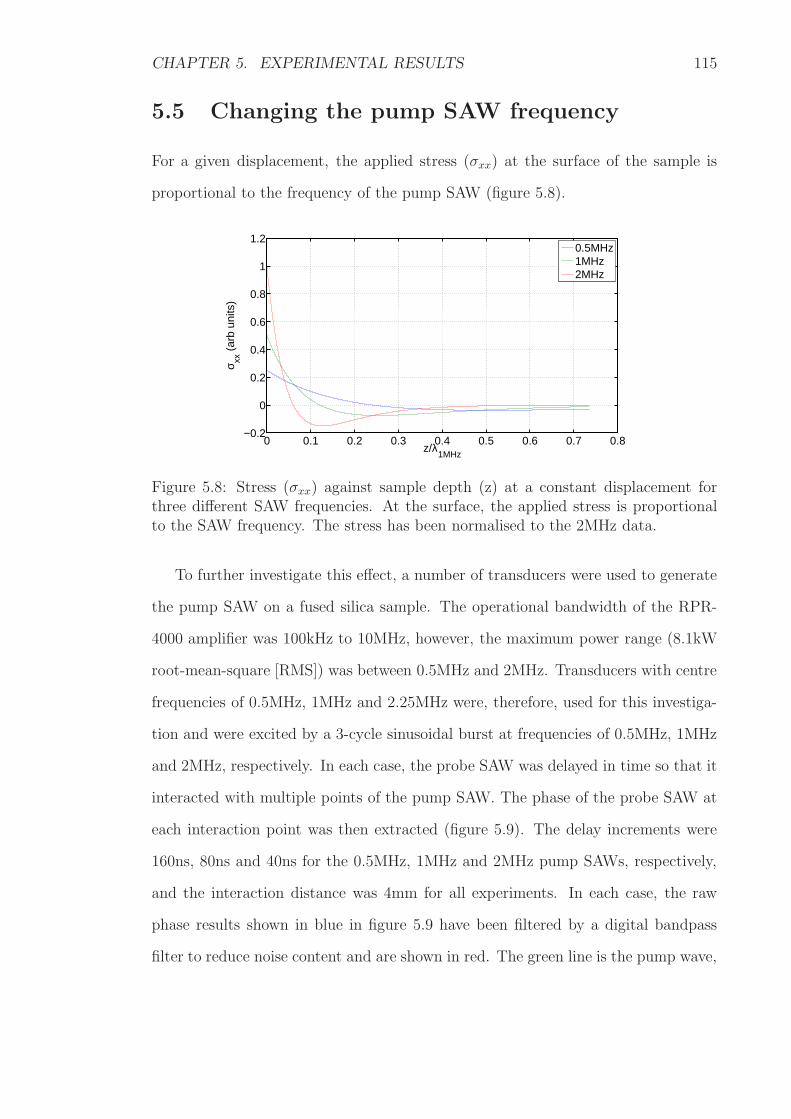
CHAPTER 5. EXPERIMENTAL RESULTS 115
5.5 Changing the pump SAW frequency
For a given displacement, the applied stress (σxx) at the surface of the sample is
proportional to the frequency of the pump SAW (figure 5.8).
0 0.1 0.2 0.3 0.4 0.5 0.6 0.7 0.8−0.2
0
0.2
0.4
0.6
0.8
1
1.2
z/λ1MHz
σ xx (
arb
units
)
0.5MHz1MHz2MHz
Figure 5.8: Stress (σxx) against sample depth (z) at a constant displacement forthree different SAW frequencies. At the surface, the applied stress is proportionalto the SAW frequency. The stress has been normalised to the 2MHz data.
To further investigate this effect, a number of transducers were used to generate
the pump SAW on a fused silica sample. The operational bandwidth of the RPR-
4000 amplifier was 100kHz to 10MHz, however, the maximum power range (8.1kW
root-mean-square [RMS]) was between 0.5MHz and 2MHz. Transducers with centre
frequencies of 0.5MHz, 1MHz and 2.25MHz were, therefore, used for this investiga-
tion and were excited by a 3-cycle sinusoidal burst at frequencies of 0.5MHz, 1MHz
and 2MHz, respectively. In each case, the probe SAW was delayed in time so that it
interacted with multiple points of the pump SAW. The phase of the probe SAW at
each interaction point was then extracted (figure 5.9). The delay increments were
160ns, 80ns and 40ns for the 0.5MHz, 1MHz and 2MHz pump SAWs, respectively,
and the interaction distance was 4mm for all experiments. In each case, the raw
phase results shown in blue in figure 5.9 have been filtered by a digital bandpass
filter to reduce noise content and are shown in red. The green line is the pump wave,

CHAPTER 5. EXPERIMENTAL RESULTS 116
which has been normalised with the phase measurements. At each frequency, there
is a clear correlation between the phase measurements and the corresponding pump
SAW wave packet.
The unfiltered phase data from figure 5.9 has been plotted against displacement
in figure 5.10(a). In figure 5.10(b), the phase measurements have been converted to
velocity and lines have been fitted to these data (figure 5.10(c)).
In order to compare the three sets of data, the results were plotted in terms
of velocity and stress (figure 5.11(a)). Although the velocity-stress gradients are
expected to be the same for all cases, the value obtained for the 0.5MHz SAW pump
frequency was higher than those from 1MHz and 2MHz frequencies (table 5.1).
SAW pump Frequency (MHz) Gradient (mms−1/MPa)0.5 139.3±3.91 122.4±5.12 126.5±10.4
Table 5.1: Velocity-stress gradients acquired from figure 5.11(b) for different pumpSAW frequencies.
The reason for this discrepancy was because the output from the 0.5MHz trans-
ducer was not constant over the duration of the experiment.
For these nonlinear experiments it is important to acquire both the pump and
probe traces at each delay, so that the probe phase modulation can be related to
surface stress. A single experiment was performed in three parts.
1. Detect pump and probe simultaneously for setting up appropriate delay range.
2. Acquire probe signals at each delay.
3. Acquire pump signals at each delay.
Parts (2) and (3) were not performed simultaneously because in order to obtain
the best possible SNR when measuring the probe pulses, it is favourable to minimise
any unnecessary splits in the detection channel. Therefore, to acquire the probe

CHAPTER 5. EXPERIMENTAL RESULTS 117
0 1 2 3 4 5 6 7 8 9 10−0.05
−0.04
−0.03
−0.02
−0.01
0
0.01
0.02
0.03
0.04
0.05
∆ΦH
F (
radi
ans)
ΦLF
(µs)
0 0.5 1 1.5 2−0.05
−0.04
−0.03
−0.02
−0.01
0
0.01
0.02
0.03
0.04
0.05
∆ΦH
F (
radi
ans)
ΦLF
(µs)
0 1 2 3 4 5 6−0.05
−0.04
−0.03
−0.02
−0.01
0
0.01
0.02
0.03
0.04
0.05
∆ΦH
F (
radi
ans)
ΦLF
(µs)
(a)
(b)
(c)
Figure 5.9: Experimental phase-modulated probe measurements on fused silica(blue) when interacting with the 0.5MHz (a), 1MHz (b) and 2MHz (c) pump SAWpackets (green) on fused silica. In each case the data have been digitally filtered inMATLAB (red).

CHAPTER 5. EXPERIMENTAL RESULTS 118
−50 −40 −30 −20 −10 0 10 20 30 40 50−0.4
−0.2
0
0.2
0.4
∆ V
HF (
ms−1
)
Displacement (nm)
−50 −40 −30 −20 −10 0 10 20 30 40 50−0.4
−0.2
0
0.2
0.4
∆ V
HF (
ms−
1 )
Displacement (nm)
−50 −40 −30 −20 −10 0 10 20 30 40 50−0.04
−0.02
0
0.02
0.04
∆ΦH
F (
radi
ans)
Displacement (nm)
(c)
(b)
(a)
Figure 5.10: Phase (a) and velocity (b) results from a fused silica sample plottedagainst surface displacement for pump frequencies of 0.5MHz (blue), 1MHz (green)and 2MHz (red). A line has been fitted to the data and is shown in (c). The rangeof displacement for the higher frequencies is smaller due to the limitations of thetransducers.

CHAPTER 5. EXPERIMENTAL RESULTS 119
−5 −4 −3 −2 −1 0 1 2 3 4 5−0.4
−0.2
0
0.2
0.4
∆ V
HF (
ms−
1 )
Stress (MPa)
−5 −4 −3 −2 −1 0 1 2 3 4 5−0.4
−0.2
0
0.2
0.4
∆ V
HF (
ms−1
)
Stress (MPa)
(b)
(a)
Figure 5.11: Velocity plotted against stress for pump frequencies of 0.5MHz (blue),1MHz (green) and 2MHz (red) (a) for fused silica. A line has been fitted to the dataand is shown in (b). The gradients of these lines are presented in table 5.1.
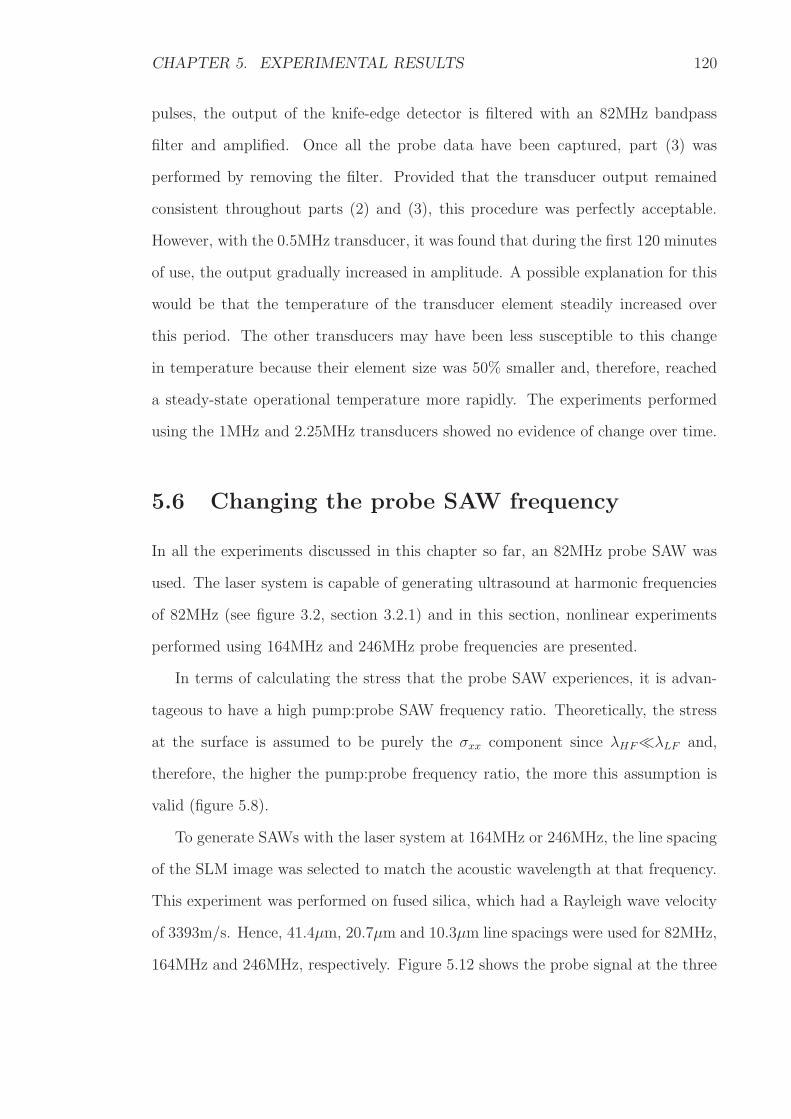
CHAPTER 5. EXPERIMENTAL RESULTS 120
pulses, the output of the knife-edge detector is filtered with an 82MHz bandpass
filter and amplified. Once all the probe data have been captured, part (3) was
performed by removing the filter. Provided that the transducer output remained
consistent throughout parts (2) and (3), this procedure was perfectly acceptable.
However, with the 0.5MHz transducer, it was found that during the first 120 minutes
of use, the output gradually increased in amplitude. A possible explanation for this
would be that the temperature of the transducer element steadily increased over
this period. The other transducers may have been less susceptible to this change
in temperature because their element size was 50% smaller and, therefore, reached
a steady-state operational temperature more rapidly. The experiments performed
using the 1MHz and 2.25MHz transducers showed no evidence of change over time.
5.6 Changing the probe SAW frequency
In all the experiments discussed in this chapter so far, an 82MHz probe SAW was
used. The laser system is capable of generating ultrasound at harmonic frequencies
of 82MHz (see figure 3.2, section 3.2.1) and in this section, nonlinear experiments
performed using 164MHz and 246MHz probe frequencies are presented.
In terms of calculating the stress that the probe SAW experiences, it is advan-
tageous to have a high pump:probe SAW frequency ratio. Theoretically, the stress
at the surface is assumed to be purely the σxx component since λHF≪λLF and,
therefore, the higher the pump:probe frequency ratio, the more this assumption is
valid (figure 5.8).
To generate SAWs with the laser system at 164MHz or 246MHz, the line spacing
of the SLM image was selected to match the acoustic wavelength at that frequency.
This experiment was performed on fused silica, which had a Rayleigh wave velocity
of 3393m/s. Hence, 41.4µm, 20.7µm and 10.3µm line spacings were used for 82MHz,
164MHz and 246MHz, respectively. Figure 5.12 shows the probe signal at the three
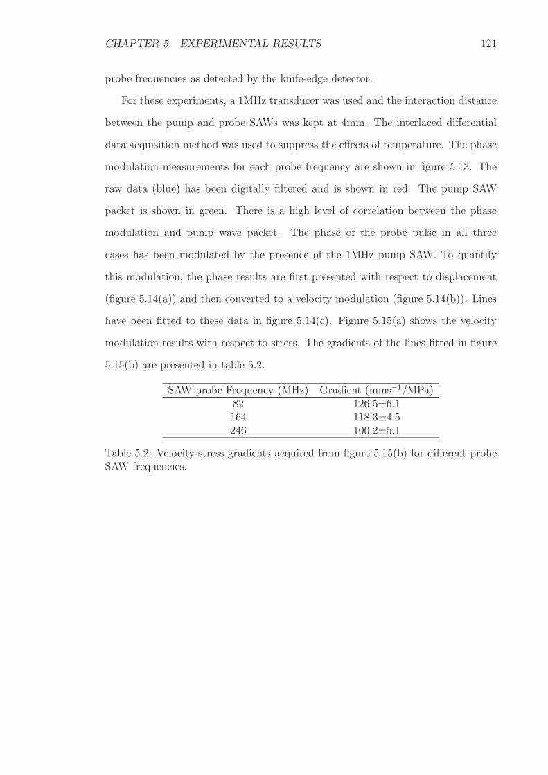
CHAPTER 5. EXPERIMENTAL RESULTS 121
probe frequencies as detected by the knife-edge detector.
For these experiments, a 1MHz transducer was used and the interaction distance
between the pump and probe SAWs was kept at 4mm. The interlaced differential
data acquisition method was used to suppress the effects of temperature. The phase
modulation measurements for each probe frequency are shown in figure 5.13. The
raw data (blue) has been digitally filtered and is shown in red. The pump SAW
packet is shown in green. There is a high level of correlation between the phase
modulation and pump wave packet. The phase of the probe pulse in all three
cases has been modulated by the presence of the 1MHz pump SAW. To quantify
this modulation, the phase results are first presented with respect to displacement
(figure 5.14(a)) and then converted to a velocity modulation (figure 5.14(b)). Lines
have been fitted to these data in figure 5.14(c). Figure 5.15(a) shows the velocity
modulation results with respect to stress. The gradients of the lines fitted in figure
5.15(b) are presented in table 5.2.
SAW probe Frequency (MHz) Gradient (mms−1/MPa)82 126.5±6.1164 118.3±4.5246 100.2±5.1
Table 5.2: Velocity-stress gradients acquired from figure 5.15(b) for different probeSAW frequencies.
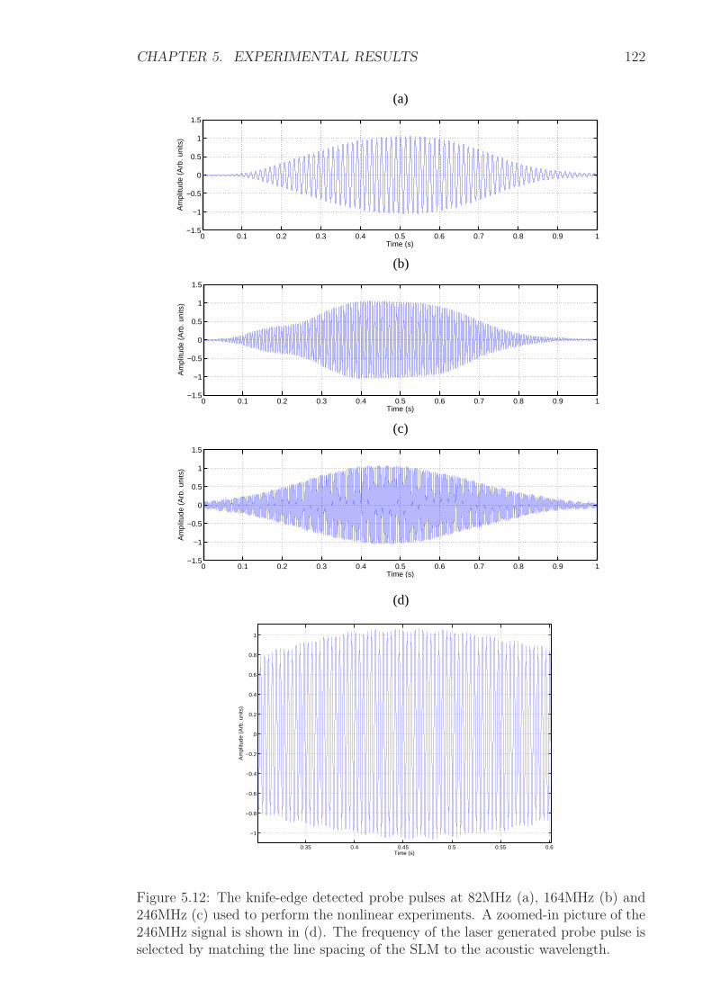
CHAPTER 5. EXPERIMENTAL RESULTS 122
0 0.1 0.2 0.3 0.4 0.5 0.6 0.7 0.8 0.9 1−1.5
−1
−0.5
0
0.5
1
1.5
Am
plitu
de (
Arb
. uni
ts)
Time (s)
0 0.1 0.2 0.3 0.4 0.5 0.6 0.7 0.8 0.9 1−1.5
−1
−0.5
0
0.5
1
1.5
Am
plitu
de (
Arb
. uni
ts)
Time (s)
0 0.1 0.2 0.3 0.4 0.5 0.6 0.7 0.8 0.9 1−1.5
−1
−0.5
0
0.5
1
1.5
Am
plitu
de (
Arb
. uni
ts)
Time (s)
0.35 0.4 0.45 0.5 0.55 0.6
−1
−0.8
−0.6
−0.4
−0.2
0
0.2
0.4
0.6
0.8
1
Am
plitu
de (
Arb
. uni
ts)
Time (s)
(a)
(b)
(c)
(d)
Figure 5.12: The knife-edge detected probe pulses at 82MHz (a), 164MHz (b) and246MHz (c) used to perform the nonlinear experiments. A zoomed-in picture of the246MHz signal is shown in (d). The frequency of the laser generated probe pulse isselected by matching the line spacing of the SLM to the acoustic wavelength.

CHAPTER 5. EXPERIMENTAL RESULTS 123
(a)
0 1 2 3 4 5 6
−0.06
−0.04
−0.02
0
0.02
0.04
0.06
ΦLF
(µs)
∆ΦH
F (
radi
ans)
(b)
0 1 2 3 4 5 6
−0.06
−0.04
−0.02
0
0.02
0.04
0.06
ΦLF
(µs)
∆ΦH
F (
radi
ans)
(c)
0 1 2 3 4 5 6
−0.06
−0.04
−0.02
0
0.02
0.04
0.06
ΦLF
(µs)
∆ΦH
F (
radi
ans)
Figure 5.13: Phase modulation measurements (blue) of the 82MHz (a), 164MHz (b)and 246MHz (c) probe frequencies. The data have been filtered and shown in red,and the pump wave packet is shown in green.

CHAPTER 5. EXPERIMENTAL RESULTS 124
−20 −15 −10 −5 0 5 10 15 20−0.2
−0.1
0
0.1
0.2
Displacement (nm)
∆ V
HF (
ms−1
)
−20 −15 −10 −5 0 5 10 15 20−0.06
−0.04
−0.02
0
0.02
0.04
0.06
Displacement (nm)
∆ΦH
F (
radi
ans)
−20 −15 −10 −5 0 5 10 15 20−0.2
−0.1
0
0.1
0.2
Displacement (nm)
∆ V
HF (
ms−1
)
(b)
(c)
(a)
Figure 5.14: Phase (a) and velocity (b) results plotted against surface displacementfor probe frequencies of 82MHz (blue), 164MHz (green) and 246MHz (red). A linehas been fitted to the data and is shown in (c).

CHAPTER 5. EXPERIMENTAL RESULTS 125
−2 −1.5 −1 −0.5 0 0.5 1 1.5 2−0.2
−0.1
0
0.1
0.2
Stress (MPa)
∆ V
HF (
ms−1
)
−2 −1.5 −1 −0.5 0 0.5 1 1.5 2−0.2
−0.1
0
0.1
0.2
Stress (MPa)
∆ V
HF (
ms−1
)
(b)
(a)
Figure 5.15: Velocity plotted against stress for probe frequencies of 82MHz (blue),164MHz (green) and 246MHz (red)(a). A line has been fitted to the data and isshown in (b). The gradients of these lines are presented in table 5.2.
CHAPTER 5. EXPERIMENTAL RESULTS 126
5.7 Comparison of nonlinear responses of fused
silica and aluminium
Previously reported findings have demonstrated that aluminium and fused silica have
opposite nonlinear responses [100, 67, 81, 4]. To validate this, nonlinear experiments
were conducted on fused silica, aluminium-2024 and aluminium-6061.
In each experiment the reference delay was set so that the probe SAW interacted
with the first peak of the pump SAW packet. This served as a marker so that at this
interaction point (reference delay), the corresponding phase measurement was known
− thus, allowing a correlation of all other phase measurements and corresponding
interaction points.
The first and last target delays were chosen so that they encapsulated the whole
of the pump wave packet (5µs in this case), and 80ns delay increments were used
so that the probe pulse interacted with 63 points on the pump wave. In order to
overcome the effects of changes in temperature on the experiments, results were
collected using the differential interlaced data capture method (see section 4.6.3).
Phase measurements for all three materials are shown in figure 5.16. The reference
delay is indicated by the red circle in each case and it has been aligned with the
first peak of the pump wave (shown in blue) so that both sets of data correspond
to each other. Clearly, the phase measurements on fused silica and aluminium are
180 out of phase, indicating that with increasing stress, the SAW velocity on one
material speeds up while on the other it slows down.
According to the literature [101], the SAW velocity on aluminium is inversely
proportional to longitudinal stress. If the velocity slows down, then the phase of
the detected signal will become more negative because it will have arrived later in
time. The results in figure 5.16 can be adjusted to show this and figure 5.17 shows
the phase modulation with actual surface displacement. The unfiltered results are
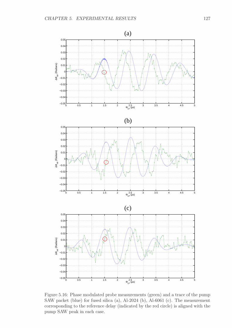
CHAPTER 5. EXPERIMENTAL RESULTS 127
0 0.5 1 1.5 2 2.5 3 3.5 4 4.5 5−0.05
−0.04
−0.03
−0.02
−0.01
0
0.01
0.02
0.03
0.04
0.05
∆ΦH
F (
Rad
ians
)
ΦLF
(µs)
0 0.5 1 1.5 2 2.5 3 3.5 4 4.5 5−0.05
−0.04
−0.03
−0.02
−0.01
0
0.01
0.02
0.03
0.04
0.05
∆ΦH
F (
Rad
ians
)
ΦLF
(µs)
0 0.5 1 1.5 2 2.5 3 3.5 4 4.5 5−0.05
−0.04
−0.03
−0.02
−0.01
0
0.01
0.02
0.03
0.04
0.05
∆ΦH
F (
Rad
ians
)
ΦLF
(µs)
(a)
(b)
(c)
Figure 5.16: Phase modulated probe measurements (green) and a trace of the pumpSAW packet (blue) for fused silica (a), Al-2024 (b), Al-6061 (c). The measurementcorresponding to the reference delay (indicated by the red circle) is aligned with thepump SAW peak in each case.
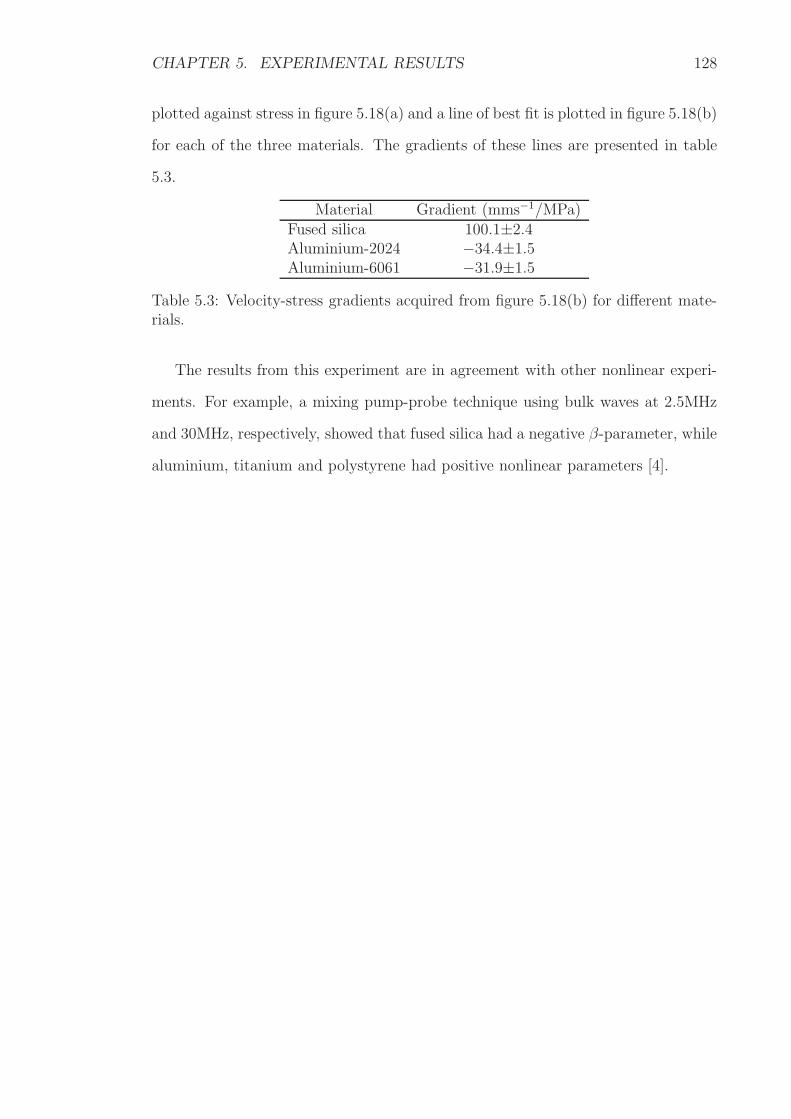
CHAPTER 5. EXPERIMENTAL RESULTS 128
plotted against stress in figure 5.18(a) and a line of best fit is plotted in figure 5.18(b)
for each of the three materials. The gradients of these lines are presented in table
5.3.
Material Gradient (mms−1/MPa)Fused silica 100.1±2.4Aluminium-2024 −34.4±1.5Aluminium-6061 −31.9±1.5
Table 5.3: Velocity-stress gradients acquired from figure 5.18(b) for different mate-rials.
The results from this experiment are in agreement with other nonlinear experi-
ments. For example, a mixing pump-probe technique using bulk waves at 2.5MHz
and 30MHz, respectively, showed that fused silica had a negative β-parameter, while
aluminium, titanium and polystyrene had positive nonlinear parameters [4].

CHAPTER 5. EXPERIMENTAL RESULTS 129
(a)
0 0.5 1 1.5 2 2.5 3 3.5 4 4.5 5−0.05
−0.04
−0.03
−0.02
−0.01
0
0.01
0.02
0.03
0.04
0.05
∆ΦH
F (
Rad
ians
)
ΦLF
(µs)
(b)
0 0.5 1 1.5 2 2.5 3 3.5 4 4.5 5−0.05
−0.04
−0.03
−0.02
−0.01
0
0.01
0.02
0.03
0.04
0.05
∆ΦH
F (
Rad
ians
)
ΦLF
(µs)
(c)
0 0.5 1 1.5 2 2.5 3 3.5 4 4.5 5−0.05
−0.04
−0.03
−0.02
−0.01
0
0.01
0.02
0.03
0.04
0.05
∆ΦH
F (
Rad
ians
)
ΦLF
(µs)
Figure 5.17: The quarter-cycle phase difference between actual and detected surfacedisplacement is removed from the results presented in figure 5.16. The phase mod-ulated probe measurements (green) and a trace of the pump SAW packet (blue) forfused silica (a), Al-2024 (b) and Al-6061 (c). The phase measurements have beenfiltered and are shown in red in each case.
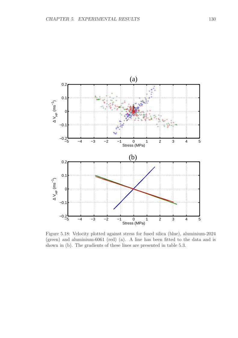
CHAPTER 5. EXPERIMENTAL RESULTS 130
−5 −4 −3 −2 −1 0 1 2 3 4 5−0.2
−0.1
0
0.1
0.2
∆ V
HF (
ms−
1 )
Stress (MPa)
−5 −4 −3 −2 −1 0 1 2 3 4 5−0.2
−0.1
0
0.1
0.2
∆ V
HF (
ms−1
)
Stress (MPa)
(a)
(b)
Figure 5.18: Velocity plotted against stress for fused silica (blue), aluminium-2024(green) and aluminium-6061 (red) (a). A line has been fitted to the data and isshown in (b). The gradients of these lines are presented in table 5.3.

CHAPTER 5. EXPERIMENTAL RESULTS 131
5.8 Nonlinear experiments with CHOTs
In each experiment described so far in this chapter, the high frequency SAW was
generated using the SLM and detected by a knife-edge detector. Here, a series of
nonlinear experiments were performed that used an alternative method to generate
and detect the probe SAW. Two experimental configurations are used in this section
and have been described in section 4.4.
1. Generation of the probe SAW using a g-CHOT and detection by a knife-edge
detector.
2. Generation of the probe SAW using a g-CHOT and detection by a d-CHOT.
During these nonlinear experiments, the interlaced differential data collection
procedure, discussed in section 4.6.3, was used so that the effects of temperature were
suppressed. The delay settings were adjusted so that the probe SAW interacted with
multiple points on the pump SAW packet, and the corresponding phase modulation
experienced by the probe SAW at each of these points was extracted. Figure 5.19(a)
and 5.19(b) shows typical probe signals generated by the g-CHOT and detected by
knife-edge or d-CHOT detection techniques.
Phase modulation results obtained for both the knife-edge and the d-CHOT
detection techniques are shown in figure 5.20(a) and 5.20(b), respectively. In both
cases the probe SAW was generated by a plane wave g-CHOT and the interaction
distance between the pump and probe SAWs was 4mm.
The pump signal shown in green in figure 5.20 indicates the stress field that the
transducer excited on the sample. Different electronic channels were used for detect-
ing the pump and probe signals. Consequently, the delay differences between the
two electronic signal paths meant that the signals’ time of arrival was also different.
For this reason, an arbitrary phase was applied to the pump wave packet so that
the probe SAW phase-modulated results coincided with their respective interaction

CHAPTER 5. EXPERIMENTAL RESULTS 132
0 0.2 0.4 0.6 0.8 1 1.2−1
−0.8
−0.6
−0.4
−0.2
0
0.2
0.4
0.6
0.8
1
Time (µs)
Am
plitu
de (
arb.
uni
ts)
0 0.2 0.4 0.6 0.8 1 1.2−1
−0.8
−0.6
−0.4
−0.2
0
0.2
0.4
0.6
0.8
1
Time (µs)
Am
plitu
de (
arb.
uni
ts)
(b)
(a)
Figure 5.19: A high-frequency SAW pulse generated by a plane wave g-CHOT anddetected by the knife-edge detector (a) and a plane wave d-CHOT (b).
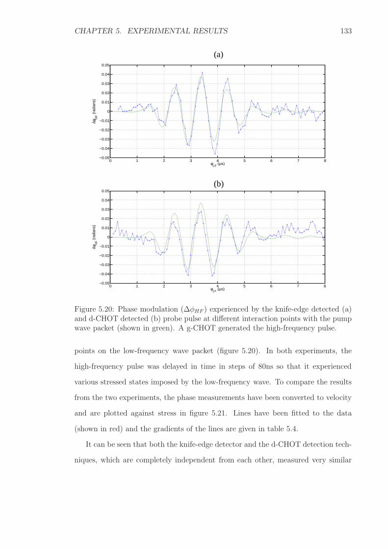
CHAPTER 5. EXPERIMENTAL RESULTS 133
0 1 2 3 4 5 6 7 8−0.05
−0.04
−0.03
−0.02
−0.01
0
0.01
0.02
0.03
0.04
0.05
φLF
(µs)
∆φH
F (rad
ians
)
0 1 2 3 4 5 6 7 8−0.05
−0.04
−0.03
−0.02
−0.01
0
0.01
0.02
0.03
0.04
0.05
φLF
(µs)
∆φH
F (rad
ians
)
(a)
(b)
Figure 5.20: Phase modulation (∆φHF ) experienced by the knife-edge detected (a)and d-CHOT detected (b) probe pulse at different interaction points with the pumpwave packet (shown in green). A g-CHOT generated the high-frequency pulse.
points on the low-frequency wave packet (figure 5.20). In both experiments, the
high-frequency pulse was delayed in time in steps of 80ns so that it experienced
various stressed states imposed by the low-frequency wave. To compare the results
from the two experiments, the phase measurements have been converted to velocity
and are plotted against stress in figure 5.21. Lines have been fitted to the data
(shown in red) and the gradients of the lines are given in table 5.4.
It can be seen that both the knife-edge detector and the d-CHOT detection tech-
niques, which are completely independent from each other, measured very similar
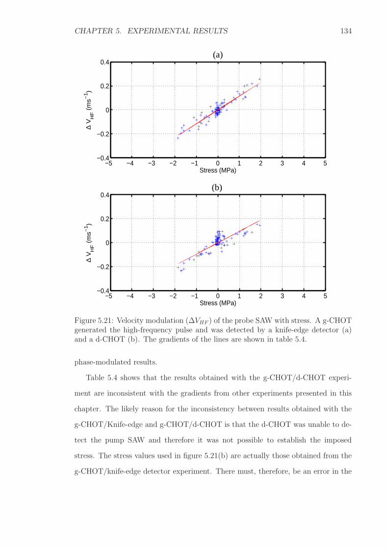
CHAPTER 5. EXPERIMENTAL RESULTS 134
−5 −4 −3 −2 −1 0 1 2 3 4 5−0.4
−0.2
0
0.2
0.4
Stress (MPa)
∆ V
HF (
ms−
1)
−5 −4 −3 −2 −1 0 1 2 3 4 5−0.4
−0.2
0
0.2
0.4
Stress (MPa)
∆ V
HF (
ms−
1)
(b)
(a)
Figure 5.21: Velocity modulation (∆VHF ) of the probe SAW with stress. A g-CHOTgenerated the high-frequency pulse and was detected by a knife-edge detector (a)and a d-CHOT (b). The gradients of the lines are shown in table 5.4.
phase-modulated results.
Table 5.4 shows that the results obtained with the g-CHOT/d-CHOT experi-
ment are inconsistent with the gradients from other experiments presented in this
chapter. The likely reason for the inconsistency between results obtained with the
g-CHOT/Knife-edge and g-CHOT/d-CHOT is that the d-CHOT was unable to de-
tect the pump SAW and therefore it was not possible to establish the imposed
stress. The stress values used in figure 5.21(b) are actually those obtained from the
g-CHOT/knife-edge detector experiment. There must, therefore, be an error in the

CHAPTER 5. EXPERIMENTAL RESULTS 135
Experimental configuration Gradient (mms−1/MPa)knife-edge detector 114.9±4.5d-CHOT 94.6±5.9
Table 5.4: Velocity-stress gradients acquired from figure 5.21 for different detectionschemes.
gradient for the g-CHOT/d-CHOT experiment.
This section has discussed how CHOTs can be incorporated into the nonlinear
experiment and has allowed for a direct comparison between two completely in-
dependent detection techniques. Both the knife-edge and d-CHOT methods have
measured similar phase modulations in the high-frequency wave.
5.9 Summary
The aim of all the experiments in this chapter was to demonstrate how nonlinear
experiments can be used to measure material nonlinearity. The series of experiments
investigating the effect of changing the pump:probe frequency ratio showed that as
the pump frequency was increased, the velocity-displacement gradient also increased
by approximately a factor of 2.
Combining CHOTs with the nonlinear experiment allowed for a direct compari-
son between two completely independent detection techniques. Both the knife-edge
and d-CHOT methods have measured similar modulations in probe velocity caused
by the stress induced by the 1MHz transducer. All the results presented in this
chapter in terms of the velocity-stress gradient are summarised in table 5.5. The
velocity-stress gradient for fused silica was relatively consistent across all nonlinear
experiments. If the results for the 0.5:82MHz and g-CHOT/d-CHOT experiments
were omitted (for reasons described in the ‘Notes’ column), then the mean velocity-
stress result is ∼115.2mms−1/MPa.
The results from nonlinear experiments showed that the relationship between
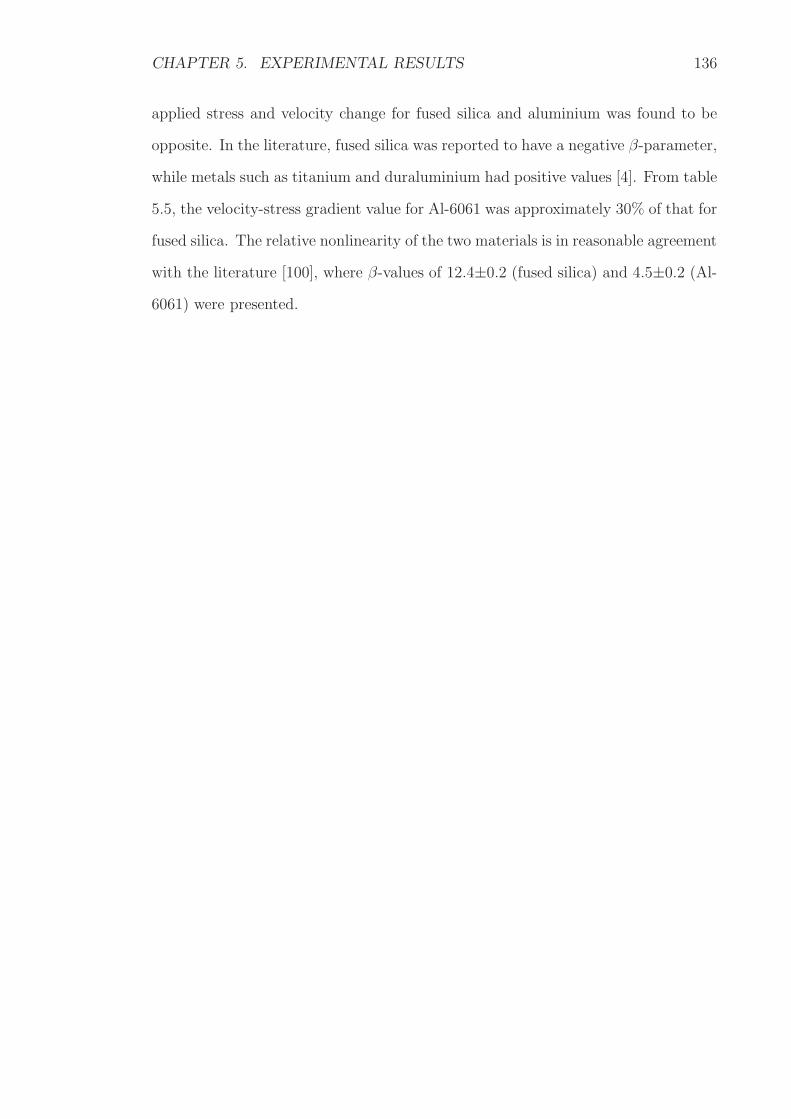
CHAPTER 5. EXPERIMENTAL RESULTS 136
applied stress and velocity change for fused silica and aluminium was found to be
opposite. In the literature, fused silica was reported to have a negative β-parameter,
while metals such as titanium and duraluminium had positive values [4]. From table
5.5, the velocity-stress gradient value for Al-6061 was approximately 30% of that for
fused silica. The relative nonlinearity of the two materials is in reasonable agreement
with the literature [100], where β-values of 12.4±0.2 (fused silica) and 4.5±0.2 (Al-
6061) were presented.
CH
AP
TE
R5.
EX
PE
RIM
EN
TA
LR
ESU
LT
S137
Nonlinear Material Pump SAW Probe SAW Gradient Notesexperiment frequency (MHz) frequency (MHz) (mms−1/MPa)
Pump SAW amplitude Fused silica 1 82 112.8±5.4changed (section 5.4)Pump SAW frequency Fused silica 0.5 82 139.3±3.9 Output from 0.5MHz transducerchanged (section 5.5) Fused silica 1 82 122.4±5.1 was not constant - possible cause of
Fused silica 2 82 126.5±10.4 error in stress measurementsProbe SAW frequency Fused silica 1 82 126.5±6.1changed (section 5.6) Fused silica 1 164 118.3±4.5
Fused silica 1 246 100.2±5.1Fused silica and Fused silica 1 82 100.1±2.4aluminium compared Al-2024 1 82 −34.4±1.5(section 5.7) Al-6061 1 82 −31.9±1.5Applied CHOTs to Fused silica (g-CHOT/Knife-edge) 1 82 114.9±4.5 Error in g-CHOT/d-CHOT experimentexperiment Fused silica (g-CHOT/d-CHOT) 1 82 94.6±5.9 since unable to detect pump SAWs(section 5.8) (Real stress values unobtainable).
Approximated by using stressmeasurements from g-CHOT/Knife-edgeexperiment
Table 5.5: Summary of results from all the experiments performed in this chapter.
Chapter 6
Conclusion and further work
The aim of this research was to develop a laser-based ultrasonic technique that could
measure material nonlinearity. The experiment used a pump-probe wave mixing
technique [2] in which the stress exerted by a pump wave caused a material velocity
change, thereby modulating the phase of the probe signal.
The work was novel because the experiment was performed using high-frequency
SAWs, generated and detected using lasers. The OSAM instrument generated the
probe SAW at frequencies of 82MHz (and its harmonics), while the pump SAW was
generated by a transducer. The ultrasound was detected by a knife-edge detector. In
addition, similar results were obtained using a g-CHOT/d-CHOT system on fused
silica.
The main difference between the technique presented here and the previously
reported methods [13, 5] is that the stress was imposed by an ultrasonic transducer,
rather than a stressing jig. Measuring velocity modulation is challenging, as only
relatively small stresses (<10MPa) can be exerted by the transducer. However,
this technique has an advantage over other methods because it could be applied to
specimens in situ i.e. the specimen would not have to be removed from its point of
operation to be placed in a jig.
Changes in laboratory temperature were found to cause velocity modulations of
138
CHAPTER 6. CONCLUSION AND FURTHER WORK 139
a similar order of magnitude as the nonlinear measurements. Ambient temperature
variations of ±1C were sufficient to engulf the measurements, so several temper-
ature suppression methods were developed to overcome this problem. The effects
of temperature were resolved by incorporating a temperature-controlled box around
the experimental apparatus and/or an electronic data acquisition system.
The principal conclusions for this work are:
1. A laser-based ultrasonic experiment has been developed and is capable of
measuring material nonlinearity. Materials that have been tested so far are
fused silica and aluminium.
2. Results showed velocity-stress gradients for fused silica, Al-2024 and Al-6061
to be +115.2mms−1/MPa, −34.4mms−1/MPa and −31.9mms−1/MPa, respec-
tively.
3. The nonlinear responses of fused silica and aluminium have been shown to be
opposite in sign, which is in agreement with the literature.
Further work includes the application of this nonlinear experiment to more ‘dif-
ficult’ materials such as titanium, which is commonly used in aircraft engine compo-
nents. As the grain structure of titanium can cause 82MHz SAWs to be aberrated
[102], one of two existing aberration correction techniques would have to be applied
[96], in order to perform a nonlinear experiment on this difficult material.
To validate the results presented in this thesis, it is important to compare the
results with those obtained using different experimental techniques, such as the
mechanically applied stress method described in [13] for example. The materials that
were used in each case were different and so in order to have a direct comparison,
nonlinear experiments on steel and silicon nitride samples need to be performed.
The main advantages that CHOTs have over the SLM/knife-edge detector sys-
tem are the greatly reduced cost and complexity of the optical setup required to
CHAPTER 6. CONCLUSION AND FURTHER WORK 140
perform experiments. Although no experiments have been performed using CHOTs
on metals, to-date, this is a potential application. In order to generate ultrasound
on aluminium for example, the lines of the g-CHOT would have to be made of a
material that has either a lower or higher absorption coefficient. Provided that there
is a sufficient absorption contrast between the two materials, either of these options
would be suitable. The use of a g-CHOT to generate the low-frequency SAW on
the test material would have the advantage of making this nonlinear experiment
completely non-contact. In order to get the sufficiently high pump SAW amplitudes
required for the experiment, there may be a risk of causing damage to the sample
surface.
The nonlinear experiments in this thesis were performed on un-fatigued mate-
rials, but with a view to applying it to fatigued samples. The elastic properties of
a material are affected by fatigue, which can be quantified by the velocity-stress
slope. Rolls-Royce have shown considerable interest throughout the duration of this
research and a follow-on project has been initiated with a number of academic and
industrial partners. The aim of this project is to develop a technique that can mea-
sure the residual life of aircraft engine components so that their usable life can be
safely and reliably extended. This consortium will prepare a wide range of fatigued
samples, which will then be tested using the technique described in this thesis.

Appendix A: Material Properties
Property Symbol Fused silica AluminiumRayleigh velocity (m/s) v 3393 2906Density (Pa) ρ 2200 2770Young’s Modulus (GPa) E 73 70.3Shear Modulus (GPa) µ 31 26.1
Table A1: Values used in the analysis in section 1.4.2 [63].
141

Appendix B: Brief history of the
OSAM Instrument
Over the last 15 years, the instrument we now call the OSAM has gone through
various stages of development. In 1994, a nonlinear experiment based on measuring
changes in SAW velocity caused by an applied static stress was developed [13]. These
experiments were performed on silicon nitride and steel samples. A mode-locked Q-
switched laser was used as the generation source, and the beam was focused to a
single line on the sample using a cylindrical lens. The output of the generation
system produced a short burst of SAWs at a fundamental frequency of 82MHz. The
detection system consisted of a two-beam homodyne Michelson interferometer. Each
of the two beams, which were separated by a known distance, detected the surface
displacement caused by the passing SAW. The time delay between the detected
SAW signals could then be accurately obtained and the SAW velocity determined.
Around 1996, the generation system implemented computer generated holograms
[42] and diffractive acoustic elements [103]. These holograms were capable of gen-
erating an arbitrary distribution of light onto the sample surface and therefore,
single or multiple lines or arcs could be used to generate SAWs. By using arcs, the
ultrasound was focused to a single point, which increased the SNR for the point
detection.
By 1998, it was possible to take images of the ultrasound on certain samples. The
142
APPENDIX B 143
high-speed analogue electronics that were now an integral part of the system allowed
fast acquisition of the complex amplitude of the detected ultrasound. The detection
system now consisted of a knife-edge detector. The computer-generated holograms
were then replaced by a spatial light modulator [43]. This device was computer-
controlled and could be programmed to distribute the light onto the sample in any
desired profile. The effects of aberration were then studied and techniques were
developed to correct aberration [104, 96, 105, 106, 102].
In 2003, a second OSAM system was built and was called the ARROSAM. The
work on aberration correction continued and an acoustic wavefront sensor (AWFS)
[107] was incorporated into the ARROSAM. The combination of the SLM and AWFS
meant that the higher-order aberration correction method could be implemented
more rapidly than with a single knife-edge detector.
In addition, the ARROSAM was used to develop a technique that was capable of
mapping the microstructure of multi-grained materials such as titanium alloys and
aluminium. This technique was called Spatially Resolved Acoustic Spectroscopy
(SRAS) [108, 109].
In 2003, a nonlinear technique was developed that was based on the parametric
interaction between the 82MHz SAW generated by the OSAM instrument and a low
frequency (0.5−2MHz) stressing SAW. The stress applied to the sample was found
to modulate the velocity of the 82MHz SAW [94].
Appendix C: OSAM Alignment
Introduction
There are many elements of the OSAM system that have to be aligned for maximum
efficiency. These range from simple everyday tasks, such as focusing the sample, to
more major issues, such as re-aligning the generation laser cavity. The latter is rarely
performed and is only necessary after major maintenance work has been carried out
on the laser.
Laser cavity
The three elements of the laser that are generally adjusted are the two mirrors at each
end of the laser cavity and the position of the Q-switcher crystal. The laser beam
is expanded and then projected onto a screen and a CCD camera is setup so that
the spatial properties of the beam can be observed. The aim is to adjust these laser
components to obtain a single circular beam (single mode) with a Gaussian spacial
intensity. The coherent trigger pulse ‘quality’ is a further alignment guide, as this
also provides feedback on the temporal properties of the laser. A high amplitude,
well-defined coherent trigger pulse, such as the one shown in section 3.2.1, indicates
an optimised Q-switched and mode-locked laser system has been attained.
144

APPENDIX C 145
SLM and surrounding optics
The output beam from the laser has to be directed and accurately expanded to the
appropriate size to illuminate the SLM. By keeping the laser beam orthogonal at
all times and at a consistent height above the optical table (∼10cm), alignment is
generally made easier. Once aligned, the first half-wave plate and beam expander
system are fixed into place and are rarely adjusted. The optical components enclosed
by the dashed box in figure 3.1 (section 3.2) are attached to the same fixture so that
there is no relative movement between them. The individual components within
it can, however, be adjusted. For example, both beam splitters can be rotated
and tilted, the halfwave plate can be easily rotated, the beam block position in
the horizontal and vertical planes can be adjusted so that the appropriate area of
the SLM is illuminated and the CCD camera can be removed when necessary to
accommodate the placement of the temperature controlled box (section 4.6.1). The
SLM head is mounted independently on a mechanical stage so that its distance
from the sample can be adjusted. It also has in-built tip/tilt adjustments for precise
positioning.
Sample
There are three main components of the OSAM instrument that have to be in focus
with the sample and, therefore, in focus with each other. These are the SLM, the
detection system and the imaging (CCD camera) system. If any one of these is in
focus with the sample initially, then the task of aligning the other two parts is made
much easier. If this is not the case, and all parts are out of focus, then the alignment
process becomes more complicated. This section details the general procedure that
was used when the OSAM was in a state of complete mis-alignment.
In order to have the best possible chance of aligning the system, an ‘ideal’ sample
APPENDIX C 146
is used. This is a flat, smooth, polished mirror with a known velocity (2952m/s).
The sample should have one or two scratches as these will be used to focus the CCD
camera onto the sample.
The sample scratches are first illuminated by a torch or LED, and the CCD
camera position (relative to the sample) is adjusted. When the image of the scratches
looks sharp on the camera system, it means that the camera and sample are in focus.
An SLM image is uploaded to the SLM, consisting of a series of plane lines. The
line spacing is chosen to match the acoustic wavelength of the sample which is 36µm
for an ideal sample. Plane SAWs are used at this stage as there is a greater chance
of detecting a signal than with focused waves. Any mis-alignment (which is very
probable at the early stages of the alignment process) means it is unlikely that the
location of the arc focus is precisely where the detection probe is situated, whereas
the detector position is less critical with plane waves.
The SLM position is then adjusted so that the lines become sharp and clearly
defined on the CCD camera image. At this point both the SLM and camera are in
focus with the sample. If required, the halfwave plate in front of the SLM can be
rotated at this stage so that the maximum contrast between light and dark lines of
the SLM image is achieved.
The next stage is to get the detector system into focus with the sample. Any
scratches, patches of dust or even a finger print present on the surface of the sample
will cause the light from the detection laser to be scattered. In order to see the
spurious reflections, a white card is temporarily held in front of the sample. The
sample position is then moved until these reflections appear sharp and in focus on
the white card. When this is achieved, the sample and detector system are in focus.
The focusing lens situated directly in front of the knife edge detector can then
be positioned so that the light is shared equally between the two photodiodes. Fi-
nally, the SLM line spacing is adjusted to confirm that the 82MHz SAWs are most

APPENDIX C 147
efficiently generated at a line spacing of 36µm.
Bibliography
[1] SD Sharples, M Clark, and MG Somekh. All-optical adaptive scanning acous-
tic microscope. Ultrasonics, 41:295–299, 2003.
[2] M Vila, F Vender Meulen, S Dos Santos, L Haumesser, and O Bou Matar.
Contact phase modulation method for acoustic nonlinear parameter measure-
ment in solid. Ultrasonics, 42:1061–1065, 2004.
[3] IA Viktorov. Rayleigh and Lamb waves: physical theory and applications. New
York: Plenum Press, 1967.
[4] X Jacob, C Barriere, and D Royer. Acoustic nonlinearity parameter measure-
ments in solids using the collinear mixing of elastic waves. Applied Physics
Letters, 82(6):886–888, 2003.
[5] M Duqennoy, M Ouaftouh, and M Ourak. Determination of stresses in alu-
minium alloy using optical detection of Rayleigh waves. Ultrasonics, 37:365–
372, 1999.
[6] Lord Rayleigh. On waves propagating along the plane surface of an elastic
solid. Proceedings of the London Mathematical Society, 17:4–11, 1885.
[7] C Minton. Inspection of metals with ultrasonic surface waves. Nondestructive
Testing, 12(4):13–16, 1954.
148
BIBLIOGRAPHY 149
[8] EG Cook and HE Van Valkenburg. Surface waves at ultrasonic frequencies.
ASTM Bulletin, pages 81–84, 1954.
[9] G Alers, MA Tennison, RB Thompsom, and BR Tittmann. Visualisation of
surface elastic waves on structural materials. Ultrasonics, 11(4):174–177, 1973.
[10] R Adler, A Korpel, and P Desmares. An instrument for making surface waves
visible. IEEE Transactions on Sonics and Ultrasonics, (3):157–161, 1968.
[11] DA Cook and YH Berthelot. Detection of small surface-breaking fatigue cracks
in steel using scattering of Rayleigh waves. NDT and E International, 34:483–
492, 2001.
[12] Q Shan and RJ Dewhurst. Surface-breaking fatigue crack detection using laser
ultrasound. Applied Physics Letters, 62(21):2649–2651, 1993.
[13] MG Somekh, M Liu, HP Ho, and CW See. An accurate non-contacting laser
based system for surface wave velocity measurement. Measurement Science
and Technology, 6:1329–1337, 1995.
[14] GR Gerhart. Rayleigh wave velocity for a stress-induced slightly anisotropic
solid. Journal of the Acoustical Society of America, 60(5):1085–1088, 1976.
[15] Y Iwashimizu and O Kobori. The Rayleigh wave in a finitely deformed
isotropic elastic material. Journal of the Acoustical Society of America,
64(3):910–916, 1978.
[16] B Mi, E Michaels, and TE Michaels. An ultrasonic method for dynamic
monitoring of fatigue crack initiation and growth. 119(1):74–85, 2005.
[17] PD Warren, C Pecorari, OV Kolosov, SG Roberts, and GAD Briggs. Char-
acterisation of surface damage via surface acoustic waves. Nanotechnology,
7:295–301, 1996.
BIBLIOGRAPHY 150
[18] I Pape, CW Lawrence, PD Warren, SG Roberts, GAD Briggs, OV Kolosov,
AW Heys, CF Paines, and BK Tanner. Evaluation of polishing damage in
alumina. Philosophical Magazine A, 80(8):1913–1934, 2000.
[19] M Clark, SD Sharples, and MG Somekh. Non-contact acoustic microscopy.
Measurement Science and Technology, 11:1792–1801, 2000.
[20] M Clark, SD Sharples, and MG Somekh. Fast, all optical Rayleigh wave mi-
croscope: Imaging on isotropic and anisotropic materials. IEEE Transactions
on Ultrasonics, Ferroelectrics and Frequency Control, 47(1):65–74, 1999.
[21] P Cawley and DN Alleyne. The use of Lamb waves for the long range inspec-
tion of large structures. Ultrasonics, 34(2-5):287–290, 1996.
[22] DN Alleyne and P Cawley. The interaction of Lamb waves with defects. IEEE
Transactions on Ultrasonics, Ferroelectrics and Frequency Control, 39(3):381–
397, 1992.
[23] T Hayashi and K Kawashima. Multiple reflections of Lamb waves at a delam-
ination. Ultrasonics, 40:193–197, 2002.
[24] S Grondel, C Delebarre, J Assaad, J Dupuis, and L Reithler. Fatigue crack
monitoring of riveted aluminium strap joints by Lamb wave analysis and acous-
tic emission measurement technique. NDT and E International, 35:137–146,
2002.
[25] Z Chang and A Mal. Scattering of Lamb waves from a rivet hole with edge
cracks. Mechanics of Materials, 31:197–204, 1999.
[26] B Culshaw, G Pierce, and P Jun. Non-contact measurement of the mechanical
properties of materials using an all-optical technique. IEEE Sensors Journal,
3(1):62–70, 2003.

BIBLIOGRAPHY 151
[27] W Gao, C Glorieux, and J Thoen. Laser ultrasonic study of Lamb waves:
determination of the thickness and velocities of a thin plate. International
Journal of Engineering Science, 41:219–228, 2003.
[28] DN Alleyne and P Cawley. Optimisation of Lamb wave inspection techniques.
NDT and E International, 25(1):11–22, 1992.
[29] EA Ginzel and RK Ginzel. Ultrasonic properties of a new low attentuation
dry couplant elastomer. NDTnet, 1(2), 1996.
[30] RJ Dewhurst, CE Edwards, ADW McKie, and SB Palmer. Comparative study
of wide-band ultrasonic transducers. Ultrasonics, 25(6):315–321, 1987.
[31] PR Murray and RJ Dewhurst. A laser/EMAT system for thickness monitoring
applications using shear and l-s mode-converted waves. Measurement Science
and Technology, 12:1651–1659, 2001.
[32] Paul Mcintire. Nondestructive testing handbook Volume 7, 2nd Edition. ASNT,
1991.
[33] S Boonsang and RJ Dewhurst. Enhancement of laser
ultrasound/electromagnetic-acoustic transducer signals from Rayleigh wave
interaction at surface features. Applied Physics Letters, 82(19):3348–3350,
2003.
[34] PR Murray and RJ Dewhurst. Application of a laser/EMAT system for using
shear and ls mode converted waves. Ultrasonics, 40(1-8):771–776, 2002.
[35] GS Kino. Acoustic waves: Devices, imaging and analogue signal processing.
Prentice-Hall, 1987.
BIBLIOGRAPHY 152
[36] DC Hurley. Nonlinear propagation of narrow-band Rayleigh waves excited by
a comb transducer. Journal of the Acoustical Society of America, 106(4):1782–
1788, 1999.
[37] S Kenderian, BB Djordjevic, and RE Green. Point and line source laser gen-
eration of ultrasound for inspection of internal and surface flaws in rail and
structural materials. Research in Nondestructive Evaluation, 13:189–200, 2001.
[38] PA Doyle and CM Scala. Near-field ultrasonic Rayleigh waves from a laser
line source. Ultrasonics, 34:1–8, 1996.
[39] RJ Dewhurst and Q Shan. Optical remote measurement of ultrasound. Mea-
surement Science and Technology, 10(11):139–168, 1999.
[40] FL di Scalea, TP Berndt, JB Spicer, and BB Djordjevic. Remote laser gener-
ation of narrowband surface waves through optical fibers. IEEE Transactions
on Ultrasonics, Ferroelectrics and Frequency Control, 46(6):1551–1557, 1999.
[41] J Huang, S Krishnaswamy, and JD Achenbach. Laser generation of narrow-
band surface waves. Journal of the Acoustical Society of America, 92(5):2527–
2531, 1992.
[42] M Clark, F Linnane, SD Sharples, and MG Somekh. Frequency control in
laser ultrasound with computer generated holography. Applied Physics Letters,
72(16):1963–1965, 1998.
[43] SD Sharples, M Clark, and MG Somekh. Efficient and flexible laser ultrasound
generation using spatial light modulators. Electronics Letters, 37(18):1145–
1146, 2001.
[44] T Stratoudaki, JA Hernandez, M Clark, and MG Somekh. Cheap optical
transducers (CHOTS) for narrowband ultrasonic applications. Measurement
Science and Technology, 18:843–851, 2007.

BIBLIOGRAPHY 153
[45] JP Monchalin. Optical detection of ultrasound. IEEE Transactions on Ultra-
sonics, Ferroelectrics and Frequency Control, 33(5):485–499, 1986.
[46] AS Murfin, RA Soden, D Hatrick, and RJ Dewhurst. Laser-ultrasound detec-
tion systems: a comparative study with Rayleigh waves. Measurement Science
and Technology, 11(8):1208–1219, 2000.
[47] CB Scruby and LE Drain. Laser Ultrasonics, Techniques and Applications.
Adam Hilger, Bristol, UK, 1990.
[48] JP Monchalin. Optical detection of ultrasound at a distance using a confocal
fabry-perot interferometer. Applied Physics Letters, 47(1):14–16, 1985.
[49] JB Hoyes, Q Shan, and RJ Dewhurst. A non-contact scanning system for laser
ultrasounic defect imaging. Measurement Science and Technology, 2(7):628–
634, 1991.
[50] M Klein, B Pouet, and P Mitchell. Photo-emf detector enables laser ultrasonic
receiver. Laser Focus World, 36(8):S25–S27, 2000.
[51] L Noui and RJ Dewhurst. A laser beam deflection technique for the quanti-
tative detection of ultrasonic Lamb waves. Ultrasonics, 31(6):425–432, 1993.
[52] RL Whitman and A Korpel. Probing of acoustic surface perturbations by
coherent light. Applied Optics, 8(8):1567–1576, 1969.
[53] J Lawall and E Kessler. Michelson interferometry with 10pm accuracy. Review
of Scientific Instruments, 71(7):2669–2675, 2000.
[54] JH Yi, SH Kim, and YK Kwak. A nanometric displacement measurement
method using the detection of fringe peak movement. Measurement Science
and Technology, 11:1352–1358, 2000.

BIBLIOGRAPHY 154
[55] L Bjorno. Forty years of nonlinear ultrasound. Ultrasonics, 40(1-8):11–17,
2002.
[56] YP Zheng, RG Maev, and IY Solodov. Nonlinear acoustic applications for
material characterisation: A review. Canadian Journal of Physics, 77(12):927–
967, 1999.
[57] EN Simons. Testing of Metals. David and Charles: Newton Abbot, 1972.
[58] N Ranganathan and P Mazot. Changes in elastic constants associated with
fatigue damage in an aluminium alloy. Material Science and Engineering,
147:161–166, 1991.
[59] PB Nagy, G Blaho, and L Adler. Excess nonlinearity in materials containing
microcracks. Review of Progress in Quantitative Nondestructive Evaluation,
13:1997–1994, 1994.
[60] PB Nagy. Fatigue damage assessment by nonlinear ultrasonic materials char-
acterization. Ultrasonics, 36:375–381, 1998.
[61] PP Delsanto. Universality of nonclassical nonlinearity: Applications to non-
destructive evaluations and ultrasonics. Springer, 2007.
[62] JD Achenbach. Wave propagation in elastic solids. North-Holland, 1973.
[63] GWC Kaye and TH Laby. Tables of Physical and Chemical Constants. J
Wiley and Sons, 1993.
[64] H Ledbetter. Sound velocities, elastic constants: Temperature dependence.
Material Science and Engineering A, (442):31–34, 2006.
[65] MF Hamilton and DT Blackstock. Nonlinear Acoustics. Academic Press, 1998.

BIBLIOGRAPHY 155
[66] JK Na, JH Cantrell, and WT Yost. Linear and nonlinear ultrasound prop-
erties of fatigued 410cb stainless steel. Review of Progress in Quantitative
Nondestructive Evaluation, 15:1347–1352, 1996.
[67] RB Thompson, O Buck, and DO Thompson. Higher harmonics of finite ampli-
tude ultrasonic waves in solids. Journal of the Acoustical Society of America,
59(5):1087–1094, 1976.
[68] MA Breazeale. The ubiquitous nonlinearity: Its origin in solids. Ultrasonics
symposium, pages 1–10, 1987.
[69] O Buck, L Morris, and JM Richardson. Acoustic harmonic generation at
unbonded interfaces and fatigue cracks. Applied Physics Letters, 33(5):371–
373, 1978.
[70] DJ Barnard. Variation of nonlinearity parameter at low fundamental ampli-
tudes. Applied Physics Letters, 74(17):2447–2449, 1999.
[71] K Jhang and K Kim. Evaluation of material degradation using nonlinear
acoustic effect. Ultrasonics, 37:39–44, 1999.
[72] K Jhang. Applications of nonlinear ultrasonics to the NDE of material degra-
dation. IEEE Transactions on Ultrasonics, Ferroelectrics and Frequency Con-
trol, 47(3):540–548, 2000.
[73] A Hikata, BB Chick, and C Elbaum. Dislocation contribution to the sec-
ond harmonic generation of ultrasonic waves. Journal of Applied Physics,
36(1):229–236, 1965.
[74] JH Cantrell and WT Yost. Nonlinear ultrasonic characterisation of fatigue
microstructures. International Journal of Fatigue, 23:S487–S490, 2001.

BIBLIOGRAPHY 156
[75] EGH Lean, CC Tseng, and CG Powell. Optical probing of acoustic surface-
wave harmonic generation. Applied Physics Letters, 16(1):32–35, 1970.
[76] DC Hurley and CM Fortunko. Determination of the nonlinear ultrasonic pa-
rameter b using a Michelson interferometer. Measurement Science and Tech-
nology, 8:634–642, 1997.
[77] A Moreau. Detection of acoustic second harmonics in solids using a heterodyne
laser interferometer. Journal of the Acoustical Society of America, 98(5):2745–
2752, 1995.
[78] J Herrmann, J Kim, LJ Jacobs, J Qu, JW Littles, and MF Savage. Assessment
of material damage in a nickel-base superalloy using nonlinear Rayleigh surface
waves. Journal of Applied Physics, 99(12):Art. No. 124913, 2006.
[79] JL Blackshire, S Sathish, J Na, and J Frouin. Nonlinear laser ultrasonic
measurements of localized fatigue damage. Review of Quantitative Evaluation,
22:1479–1487, 2003.
[80] J Frouin, S Sathish, TE Matikas, and JK Na. Ultrasonic linear and nonlinear
behaviour of fatigued Ti-6Al-4V. Journal of Materials Research, 14(4):1295–
1298, 1999.
[81] P Li, WP Winfree, WT Yost, and JH Cantrell. Observation of collinear beam-
mixing by an amplitude modulated ultrasonic wave in a solid. In 1983 Ultra-
sonics Symposium, pages 1152–1156, 1983.
[82] KEA Van den Abeele, PA Johnson, and AM Sutin. Nonlinear elastic wave
spectroscopy (NEWS) techniques to discern material damage, part 1: Non-
linear wave modulation spectroscopy (NWMS). Research in nondestructive
evaluation, 12(1):17–30, 2000.

BIBLIOGRAPHY 157
[83] DM Donskoy and AM Sutin. Vibro-acoustic modulation nondestructive eval-
uation technique. Journal of Intelligent Material Systems and Structures,
9(9):765–771, 1998.
[84] AM Sutin and DM Donskoy. Vibro-acoustic modulation nondestructive eval-
uation technique. In Conference on Nondestructive Evaluation of Aging Air-
craft, pages 226–237, 1998.
[85] KEA Van den Abeele, AM Sutin, J Carmeliet, and PA Johnson. Micro-damage
diagnostics using nonlinear elastic wave spectroscopy (NEWS). NDT and E
International, 34(4):239–248, 2001.
[86] V Zaitsev and P Sas. Nonlinear response of a weakly damaged metal sample:
A dissipative modulation mechanism of vibro-acoustic interaction. Journal of
Vibration and Control, 6(6):803–822, 2000.
[87] V Yu Zaitsev, AM Sutin, I Yu Belyaeva, and VE Nazarov. Nonlinear in-
teraction of acoustical waves due to cracks and its possible usage for crack
detection. Acoustical Physics, 46(4):427–432, 2000.
[88] D Donskoy, A Sutin, and A Ekimov. Nonlinear acoustic interaction on contact
interfaces and its use for nondestructive testing. NDT and E International,
34(4):231–238, 2001.
[89] AM Sutin and DM Donskoy. Nonlinear vibro-acoustic nondestructive testing
technique. In 8th International Symposium on Nondestructive Charaterisation
of Materials, pages 133–138, 1998.
[90] Z Yan and PB Nagy. Thermo-optical modulation for improved ultrasonic
fatigue crack detection in Ti-6A1-4V. NDT and E International, 33:213–223,
2000.

BIBLIOGRAPHY 158
[91] P le Bas, K Van Den Abeele, S Dos Santos, T Goursolle, and O Bou Matar.
Experimental analysis for nonlinear time reversal imaging of damaged mate-
rials. In 9th European conference on NDT, Berlin, 2006.
[92] K Van Den Abeele, T Kathowski, and C Mattei. Nonlinear acoustic and ultra-
sonic NDT of aeronautical components. In Innovations in Nonlinear Acoustics:
17th International Symposium on Nonlinear Acoustics, pages 75–78, 2006.
[93] SD Sharples. All-optical scanning acoustic microscope. PhD thesis, The Uni-
versity of Nottingham, 2003.
[94] IJ Collison, T Stratoudaki, M Clark, and MG Somekh. Measurement of elastic
nonlinearity using remote laser ultrasonics and CHeap optical transducers and
dual frequency surface acoustic waves. Ultrasonics, in press.
[95] ED Palik. Handbook of optical constants of solids. London: Academic Press,
1998.
[96] SD Sharples, M Clark, and MG Somekh. Dynamic higher-order correction of
acoustic aberration due to material microstructure. Applied Physics Letters,
81(12):2288–2290, 2002.
[97] IJ Collison, T Stratoudaki, M Clark, and MG Somekh. Measurement of elas-
tic nonlinearity using remote laser ultrasonics with CHeap optical transducers
and dual frequency surface acoustic waves. In International Congress on Ul-
trasonics, 2007.
[98] K Salama and CK Ling. The effect of stress on the temperature dependence
of ultrasonic velocity. Journal of Applied Physics, 51(3):1505–1509, 1980.
[99] LG Parratt. Probability and experimental errors in science: an elementary
survey. Dover Publications, inc. New York, 1961.
BIBLIOGRAPHY 159
[100] GE Dace, RB Thompson, and O Buck. Measurement of the acoustic harmonic
generation for materials characterization using contact transducers. Review of
Progress in Quantitative Nondestructive Evaluation, 11:1685–1692, 1991.
[101] M Kato, T Sato, and K Ando. Determination of the higher-order elastic
compliance constants of metals from measurements of the dependence of ul-
trasound velocity on stress. Journal of the Acoustical Society of America,
101(4):2111–2121, 1997.
[102] SD Sharples, M Clark, IJ Collison, and MG Somekh. Adaptive acoustic imag-
ing using aberration correction in difficult materials. Insight, 47(2):78–80,
2005.
[103] SD Sharples, M Clark, and MG Somekh. Noncontact continuous wave-
front/diffractive acoustic elements for Rayleigh wave control. Electronics Let-
ters, 74(24):3604–3606, 1999.
[104] SD Sharples, M Clark, and MG Somekh. All-optical adaptive scanning acous-
tic microscope. Ultrasonics, 41(4):295–299, 2003.
[105] IJ Collison, SD Sharples, M Clark, and MG Somekh. Adaptive correction for
acoustic imaging in difficult materials. In Review of Progress in Quantitative
Nondestructive Evaluation, volume 24A and 24B 760, pages 1616–1621, 2005.
[106] JA Hernandez, M Clark, IJ Collison, M Somekh, and SD Sharples. Statis-
tical characterisation of metals from ultrasonic aberrations. In 2005 IEEE
Ultrasonics Symposium, volume 1-4, pages 1139–1142, 2005.
[107] SD Sharples, M Clark, and MG Somekh. Surface acoustic wavefront sensor
using custom optics. Ultrasonics, 42:647–651, 2004.
BIBLIOGRAPHY 160
[108] SD Sharples, M Clark, and MG Somekh. Fast noncontact imaging of ma-
terial microstructure using local surface acoustic wave velocity mapping. In
Proceedings of 2005 IEEE Ultrasonics Symposium, pages 886–889, 2005.
[109] SD Sharples, M Clark, and MG Somekh. Spatially resolved acoustic spec-
troscopy for fast noncontact imaging of material microstructure. Optics ex-
press, 14(22):10435–10439, 2006.


![Review of Laser-Generated Ultrasound Transmitters and ...€¦ · High intensity focused ultrasound (HIFU) is valuable for therapeutic applications [15,16]. Its applications featuring](https://static.fdocuments.in/doc/165x107/5f0d02697e708231d4383a2a/review-of-laser-generated-ultrasound-transmitters-and-high-intensity-focused.jpg)
![Laser-Generated Ultrasound [Good for Theory]](https://static.fdocuments.in/doc/165x107/5447ea7ab1af9f57618b46ad/laser-generated-ultrasound-good-for-theory.jpg)