MEASUREMENT OF LAMINAR BURNING SPEED AND FLAME INSTABLITY STUDY OF

SYNGAS/OXYGEN/HELIUM PREMIXED FLAME 

A Thesis presented

By

Ziyu Wang

to

The Department of Mechanical and Industrial Engineering

in partial fulfillment of the requirements for the degree of

Master of Science

in the field of

Thermo-fluids, Mechanical Engineering

Northeastern University Boston, Massachusetts

May 2016

ii  

ACKNOWLEDGEMENTS

I would like to express my thanks to my advisor Professor Hameed Metghalchi for all of

his guidance and assistance during both times of coursework and research. I also want to

thank the lab team for all the effort put into this research and the help offered to me; Omid

Askari, Kevin Vien, Matteo Sirio, Mohammed Alswat, Guangying Yu, Matthew Ferrari

and Mimmo Elia. Without your help I wouldn’t be where I am today.

Next, I want to thank all my professors who teach me the most challenging courses and

answer me questions. I want to thank all my friends who are studying and playing with me

together.

Finally, I must thank my parents for affording me the opportunity to attend Northeastern

University and all of their unfailing support and love over the years. And to my girlfriend

Alicea for your love and encouragement when I needed it the most.

 

iii  

ABSTRACT

Synthesis gas also known as syngas, which is a mixture of hydrogen and carbon monoxide

have been expected to play an important role in future energy demand. Research studies

into understanding the knowledge of its fundamental thermo-physical properties, such as

laminar burning speed, flame structure, etc. are extremely relevant in internal combustion

engine, gas turbine combustor and power plant. The aim of this thesis is to measure laminar

burning speed and study flame instability of syngas/oxygen/helium mixtures. Different

methods of measurement of laminar burning speed have been discussed in this thesis. In

present works, the experiments were conducted in a constant volume cylindrical chamber

coupled with a Z-shaped Schlieren/shadowgraph system. Pressure rise data during the

flame propagation was obtained through pressure transducers on the cylindrical chamber

wall and was a primary input into the thermodynamic model used to measure the laminar

burning speed. A high speed CMOS camera capable of taking pictures up to 40,000 frames

per second can be used to determine the stability of the flames. A syngas with different

hydrogen concentrations (5%, 10% and 25%) have been used in this experiment. The

laminar burning speed and flame instability of spherically expanding flames of syngas with

oxygen/helium have been studied over a wide range of equivalence ratios (0.6, 1, 2 and 3),

initial mixture temperatures (298 K, 400 K and 480 K) and initial pressures (0.5 atm, 1 atm

and 2 atm). Based on these initial conditions, laminar burning speed has been measured for

temperatures ranging from 298 K to 650 K, pressures between 0.5 to 7.3 atmospheres and

iv  

equivalence ratios ranging from 0.6 to 3.0. The flame instabilities have been observed

during flame propagation and considered into hydrodynamic and diffusive-thermal effects.

Helium increases the stability of flame, and it has larger heat capacity ratio (γ=1.67) than

nitrogen (γ=1.40). Those are the reasons why helium was used instead of nitrogen to

increase the range of laminar burning speed measurement that can be used for kinetic

validation. Data shows that the laminar burning speed of oxygen/helium is also higher than

oxygen/nitrogen from the results in this thesis.

v  

TABLE OF CONTENTS 1 Introduction ................................................................................................................. 1

1.1 Background .......................................................................................................... 1

1.2 Different Experimental Methods of Measuring Burning Speed .......................... 3

1.3 H2/CO (Syngas) with Helium Diluent .................................................................. 6

2 Experimental Facility and Procedure .......................................................................... 9

2.1 Cylindrical Combustion Chamber ........................................................................ 9

2.2 Gas Delivery System .......................................................................................... 11

2.3 Heating System .................................................................................................. 13

2.4 Ignition System .................................................................................................. 15

2.5 Schlieren/Shadowgraph System ......................................................................... 17

2.6 Experimental Procedure ..................................................................................... 19

3 Burning Speed Model ................................................................................................ 21

3.1 Burned Gas Mass Fraction and Temperature ..................................................... 23

3.2 Burning Speed, Flame Speed and Gas Speed .................................................... 27

4 Results and Discussion .............................................................................................. 29

4.1 Range of Conditions Tested ............................................................................... 29

4.2 Flame Structure and Instability Study ................................................................ 29

4.3 Stretch effect investigation ................................................................................. 35

4.4 Data Processing .................................................................................................. 38

4.5 Laminar Burning Speed ..................................................................................... 40

5 Conclusions ............................................................................................................... 45

REFERENCE .................................................................................................................... 46 

 

vi  

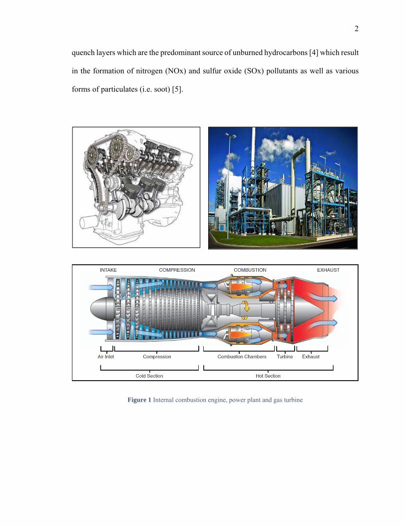
LIST OF FIGURES  Figure 1 Internal combustion engine, power plant and gas turbine ................................... 2 

Figure 2 Schematic of cylindrical chamber ..................................................................... 10 

Figure 3 Cylindrical chamber with two band heaters ...................................................... 10 

Figure 4 Gas delivery system and pressure gauges .......................................................... 12 

Figure 5 Electrical schematic for heating system ............................................................ 13 

Figure 6 AT-BBA-200 PID controllers for band heaters ................................................. 14 

Figure 7 Extended length spark plugs .............................................................................. 16 

Figure 8 A Z-type Schlieren/Shadowgraph system ......................................................... 18 

Figure 9 Schematic of three different zones in the thermodynamics model .................... 22 

Figure 10 Pictures of the H2/CO/O2/He flames for different equivalence ratios and hydrogen percentages, initial temperature of 400 K, initial pressure of 2.0 atm, and at the same flame radius ............................................................................................................. 32 

Figure 11 Pictures of the H2/CO/O2/He flames for different pressures and temperatures, hydrogen percentage of 25%, equivalence ratio at 2.0, and at the same flame radius ..... 33 

Figure 12 Pictures of the H2/CO/O2/diluent flames for different diluents of nitrogen and helium, initial temperature 298 K, initial pressure 2.0 atm, equivalence ratio 1.0, and at the same radius........................................................................................................................ 34 

Figure 13 Isentropic plot of different initial temperatures at hydrogen concentration 5%, initial pressure 0.5 atm, and equivalence ratio 2.0 ............................................................ 36 

Figure 14 Laminar burning speed of different initial temperatures (stretch rates) at hydrogen concentration 5%, initial pressure 0.5 atm, and equivalence ratio 2.0 ............. 37 

Figure 15 Pressure data of hydrogen concentration 5%, initial pressure 1.0 atm, equivalence ratio 2.0, and initial temperature 400 K ........................................................ 39 

Figure 16 Laminar burning speed of different equivalence ratios at hydrogen concentration of 5%, initial pressure 1.0 atm, and initial temperature 400 K ......................................... 41 

Figure 17 Laminar burning speed of different equivalence ratios at hydrogen concentration of 5%, initial pressure 1.0 atm, and initial temperature 480 K ......................................... 41 

Figure 18 Laminar burning speed of different hydrogen concentrations at initial pressure 1.0 atm, equivalence ratio 1.0, and initial temperature 400 K .......................................... 42

 

vii  

Figure 19 Laminar burning speed of different hydrogen concentrations at initial pressure 1.0 atm, equivalence ratio 1.0, and initial temperature 480 K .......................................... 42 

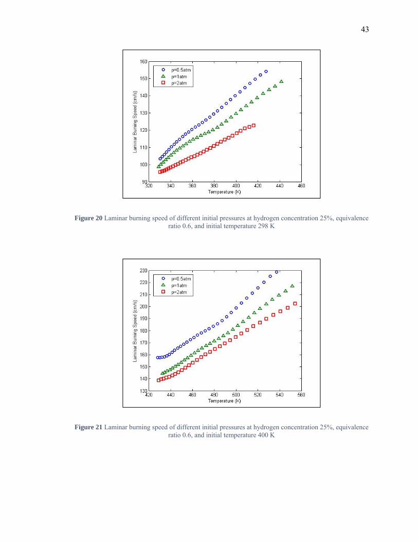
Figure 20 Laminar burning speed of different initial pressures at hydrogen concentration 25%, equivalence ratio 0.6, and initial temperature 298 K ............................................... 43 

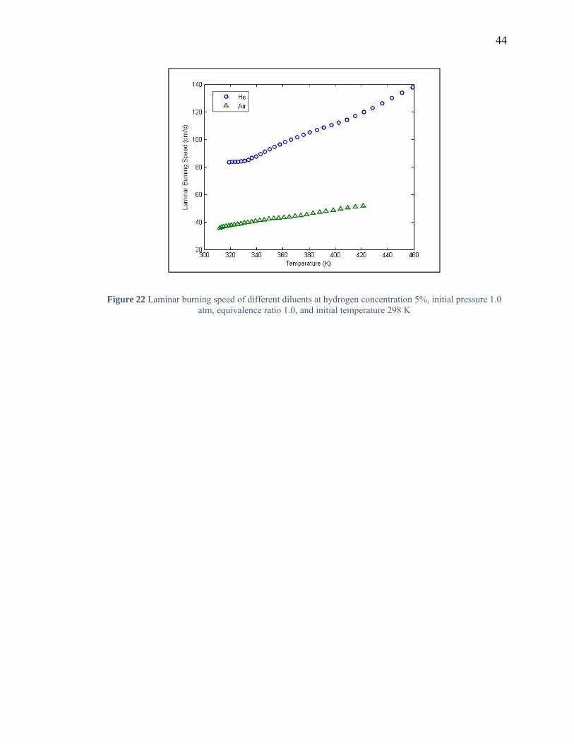
Figure 21 Laminar burning speed of different initial pressures at hydrogen concentration 25%, equivalence ratio 0.6, and initial temperature 400 K ............................................... 43 

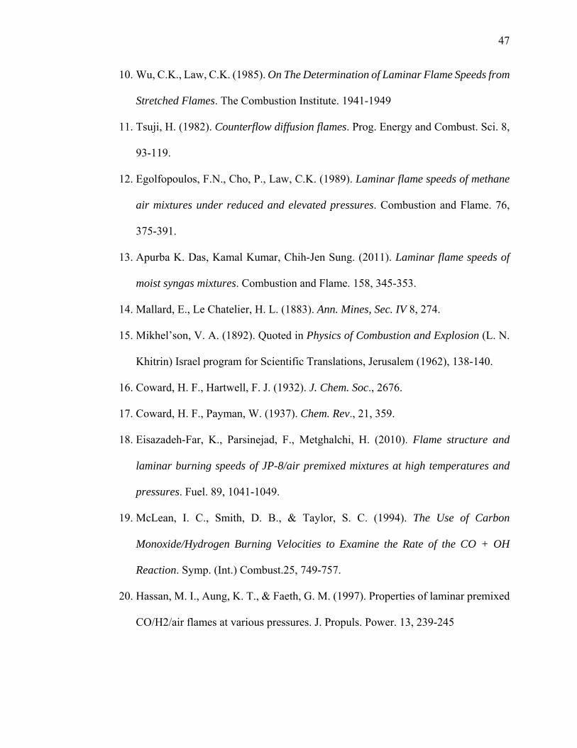
Figure 22 Laminar burning speed of different diluents at hydrogen concentration 5%, initial pressure 1.0 atm, equivalence ratio 1.0, and initial temperature 298 K ................. 44 

1  

1 Introduction

In this section, an overview of the significance of laminar burning speed to the combustion

study is given alongside a brief review of the methods of measurement of this thermo-

physical property. Additionally a slight overview of synthetic gas and oxygen/helium at

evaluated temperature comparing with oxygen/nitrogen is also presented in this research.

1.1 Background

Research studies of the laminar burning speed and flame structure of combustion are

critically significant for the development of fluid dynamic models studying fuel oxidation

and chemical kinetic both of which directly impact everyday applications involving fuel

use in different engines, power plants, and chemical processors. The study of laminar

burning speed at high temperatures and pressures is of utmost importance for predicting

and analyzing the performance of internal combustion engines, gas turbine combustors and

power plants, presented in Figure 1, in the continuing effort to improve overall efficiency

and reduce pollutant emissions.

Laminar burning speed is a thermo-physical property that is the direct measurement of the

rate of energy released during the combustion process of any combustible mixture and is a

direct function of pressure, temperature, equivalence ratio, diluent type and fuel

composition. Physically, laminar burning speed is defined as the rate of expansion at which

a planar, one-dimensional, adiabatic flame front travels relative to the unburned gas

mixture. Laminar burning speed is also used as a primary input alongside adiabatic flame

temperature for many turbulent combustions and wall quenching models [1-3]. With regard

to internal combustion engines, for example, the laminar burning speed of a fuel-oxidizer

mixture is of practical interest as it allows for the determination of the thickness of the wall

2  

quench layers which are the predominant source of unburned hydrocarbons [4] which result

in the formation of nitrogen (NOx) and sulfur oxide (SOx) pollutants as well as various

forms of particulates (i.e. soot) [5].

 

 

Figure 1 Internal combustion engine, power plant and gas turbine

3  

1.2 Different Experimental Methods of Measuring Burning Speed

The experimental techniques employed in the measurement of laminar burning speed can

be generally categorized into two general methods based on flame type: stationary flames

method and propagating flames method. A brief overview has been provided of two most

widely used methods for convenience and it is not intended to be a complete summary for

the various methods developed by different researchers. Reviews of many past

methodologies of laminar burning speed are given in the literature such as those by Linnett

[6], Andrews and Bradley [7], and Rallis and Garforth [8].

Stationary flames method encompass those such as flat flame burners, nozzle burners, and

stagnation flames. In flat flame burners, a stream of fuel flows into the stationary flame,

thus the speed at which the unburned gas enters the stable flame burner is equal to the

laminar burning speed of that fuel. The flat flame burners use a lot of the vertical channels

to make sure the flames are flat. But, flat flame burners typically have a drawback that is a

lack of consistency in the results of burning speed data depending on the location of the

flame. Besides, it is also limited to low burning speed (0.15-0.20m/s). Additionally, energy

losses from the flame to the burner which reduces the overall accuracy of measurement of

laminar burning speed. For this reason, Botha and Spalding have developed still flat flame

methods that use slight variations in order to circumvent the notable energy losses [9].

Researchers were able to measure the temperature rise of the cooling cover, by stabilizing

the flame on a porous plug, at different fuel flow rates. Then, they extrapolated the ratio of

volumetric flow rate to the flame disc area to determine the adiabatic flame speed.

Nozzle flames method utilize Bunsen burner type flames that are conical in shape. And

they suffer from mostly the same drawbacks as flat flame burners do. In the analysis of the

4  

conical flame, the velocity component normal to the flame surface is the burning speed at

that particular location. However, the conical flame method has several distinct drawbacks

since it cannot live up to its assumed characteristics at all time. As a result, it is very hard

to determine the real geometry of the flame by any methods. Additionally, the stretch effect

cannot be neglected because of the geometry of the flame.

The stagnation flames method also known as the counter flow method, developed by Wu

and Law [10], and used notably by Tsuji [11], and Egolfopoulos [12]. This method consists

of directing two identical and nozzle-generated flows of premixed combustible fuel normal

to each other, with an ignition source at the flows point of contact. After ignition, two

symmetrical, planar, nearly adiabatic flames are parallel on each side of the stagnation

plane generated by the impinging streams of fuel. The minimum axial velocity ahead of

the flame along the central stagnation streamline which is determined by laser Doppler

velocimetry is defined as the reference flame speed. The corresponding stretch rate can be

measured based on the radial velocity gradient at the location of the reference flame speed.

The reference flame speed data obtained for a range of stretch rates should be extrapolated

to zero stretch rate for the measurement of laminar flame speed [13]. A primary drawback

of the counter flow method is the inaccurate determination of speed profiles which are

determined numerically by extrapolating the point of zero gradient.

Propagating flames method include flame tube method and outwardly propagating

spherical flames method. The flame tube method was developed by Mallard and Le

Chatelier [14] and consists of a tube filled with a combustible mixture. The study of the

flame is obtained through a camera to capture frames at a known rate combining with the

pictures have been taken to determine the flame speed. Mikhelson [15] realized that the

5  

measured flame speed was not equal to the burning speed. The expression of the burning

speed is obtained from the mass balance of unburned gas. This expression is found

experimentally by Coward and Hartwell [16] and improved by Coward and Payman later

[17]. A primary assumption in the flame tube method is that the flame speed is constant

across any given tube cross section, however, this has been found to be a source of error.

In practice, the flame tube method suffers from quenching which is significant energy loss

from the flame to the wall of the tube, thus slowing the reported burning speed at the walls.

The reported changes in burning speed depend on the location of ignition in the tube (e.g.

was the mixture ignited from the top of bottom of the chamber). Additionally, the

experiment is affected by gravity as well.

The propagating spherical flames method can be classified into constant volume and

constant pressure approaches. The method of constant pressure propagating flames was

developed by Eisazadeh-Far and Metghalchi [18] and others [19-21]. It uses a

Schlieren/Shadowgraph system during the beginning stage of combustion, where pressure

is assumed to be constant and all species in the burned gases are assumed to be in local

thermodynamic equilibrium, this system is able to capture the ignition event and persist

through the duration of combustion. Additionally, at the onset of ignition, the flame kernel

is a constant mass system and that kernel is completely spherical. The model includes

losses due to radiation from plasma to the surroundings, energy loss associated with the

ignition source voltage drops and conduction losses to thermal boundary layers around the

spark electrodes. The inputs to the model are flame radii as a function of time which is

captured through the use of the Schlieren/shadowgraph system. However, because the

stretch effect during the beginning stage of the combustion cannot be neglected, Eisazadeh-

6  

Far [18] has a model to deal with stretch without correlation, and the others deal with the

stretch by linear or nonlinear correlation after the results have been calculated.

Constant volume propagating flames method was used by Takizawa [22] that utilizes a

thermodynamic model which calls for the input of the pressure rise as a function of time

during combustion. Laminar burning speed was calculated using the burned gas mass

fractions found by using pressure data and the linear approximation developed by Lewis

and Von Elbe in [23]. Also, in this category is a similar method developed by Metghalchi

and Keck [24]. This method also utilizes a constant volume chamber where the pressure

rise data during the combustion event is recorded. A thermodynamic model is employed

that assumes that unburned gases compress isentropically and that the burned gases are in

local thermodynamic equilibrium. The burning speed is derived from the time rate change

of the mass fraction of burned gases. The major advantage of the propagating flame method

is that it gets rid of the need for any stretch extrapolation for large radii, and that many data

points can be collected along an isentropic line in a single experiment.

1.3 H2/CO (Syngas) with Helium Diluent

In recent year, synthesis gas also known as syngas has been expected to play an important

role in future energy demand. It is a combustible mixture predominantly containing varying

levels of hydrogen and carbon monoxide and some levels of CO2, CH4, N2, and H2O and

other higher order hydrocarbons in some instances. Syngas can be produced through

various ways, for example, the gasification of coal, the gasification of biomass, steam

reforming of coke, and organic waste emissions to energy gasification. This gas is

considered an alternative fuel which is used to produce a wide range of synthetic materials,

solvents, and fertilizers. Recently a large focus has been cast on this fuel for its potential 

7  

use in the gas turbine industry as a replacement of natural gas [25-27]. Additionally, syngas

and hydrocarbon-syngas mixtures could be a proposal of the extension of flame stability

limit, the improvement of combustion performance, and the reduction of pollution such as

NOx, SOx and CO2 in different combustion systems [28]. Thus it is of utmost significance

to study the fundamental combustion characteristics of syngas to completely understand

how it behaves over a wide range of different combustion conditions. In present works, the

experiments were conducted to study the laminar burning speed and flame structure of

oxygen/helium (O2 20.95% and He 79.05%) and syngas mixture, especially at evaluated

temperature conditions (298 K to 650 K).  

There are several papers about laminar burning speed of syngas with helium diluent. Sun

et al. [25] employed a dual-chambered cylindrical apparatus to measure laminar burning

speed of H2/CO/He mixtures at atmospheric temperature, high pressures (up to 40 atm),

different hydrogen concentrations, and a range of equivalence ratios. Natarajan et al. [27]

measured laminar burning speed in a range of hydrogen percentage at reactant preheat

temperatures and pressures relevant to gas turbine combustors (up to 600 K and 15 atm).

An oxygen/helium mixture (1:9 by volume) is used as the oxidizer in order to decrease the

hydrodynamic and diffusive-thermal instabilities. Burke et al. [29] studied mass burning

rates of syngas flames at equivalence ratios from 0.85 to 2.5, flame temperatures from 1500

to 1800 K, and elevated pressures (1-25 atm) with various diluents (He, Ar, CO2). Vu et al.

[30] investigate the effects of different diluents (He, CO2, N2) of a 50:50 H2/CO mixture at

atmospheric temperature and elevated pressures.

The first reason why the helium diluent has been studied is that substitution of nitrogen in

the air with helium can increase the flame stability. The flame instabilities can be caused

8  

by body-force effect, hydrodynamic effect, and diffusive-thermal effect [30]. Comparing

with hydrodynamic and diffusive-thermal effects, the instability resulting from the body-

force effect is not significant because the body-force instability is observed only when

laminar flame speed is very small, thus this effect can be neglected [26]. Two strategies

are implemented to delay the onset of flame front instability so that the period of flame

propagation with a smooth flame surface could be extended to allow for sufficient data of

laminar flame speed that can be used for kinetic validation. The first one is using inert-

diluted mixtures (He) which increases flame thickness due to increase the adiabatic flame

temperature, and consequently decreases the development of the hydrodynamic instability.

The second one is also using helium as the diluent which increases the thermal diffusivity

of the fuel, thus, increasing the Lewis number ( / ) of the flame, which decrease

the diffusive-thermal instability [32].

The second reason why the helium diluent has been studied is that helium has larger heat

capacity ratio (γ=1.67) than nitrogen (γ=1.40). As an assumption of isentropic process has

been made for unburned gas temperature range for an experiment is extended due to the

following relation

                                                              (1) 

The high unburned gas temperature mixture is extremely relevant to internal combustion

engine, gas turbine combustor and power plants which are always working in high

unburned gas temperature condition. Furthermore, when the initial temperature increases,

the diffusive-thermal  instability hardly varies, while the hydrodynamic instability

decreases. The flames instabilities are decreased due to the decline in the hydrodynamic

instability [27]. 

9  

2 Experimental Facility and Procedure

In this section, the experimental facility used for all purposes during each experiment is

described thoroughly. It contributes to illustrate the procedure of each experiment step by

step and highlights the most critical components of the facility.

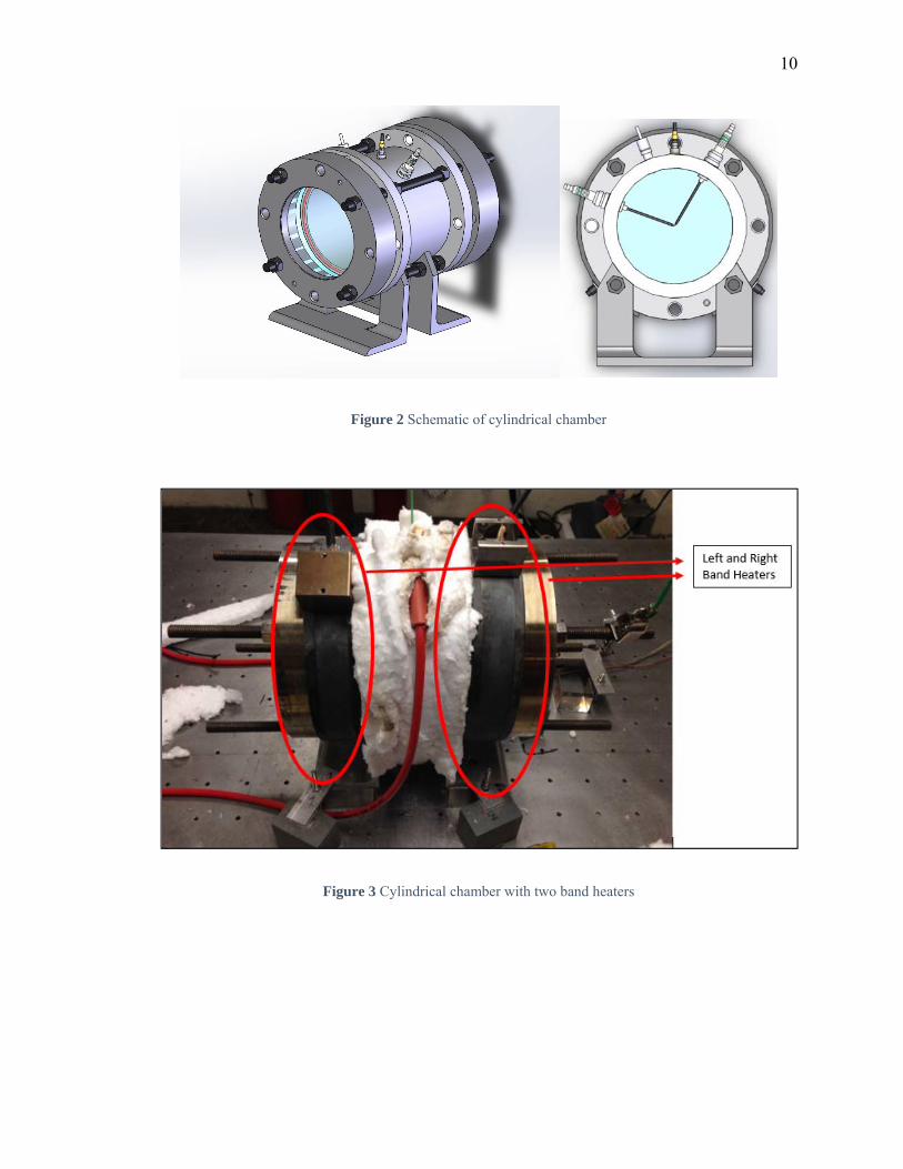
2.1 Cylindrical Combustion Chamber

The cylindrical chamber has been used in this experimentation shown in Figure 2. The

chamber has an inner diameter of 13.5 cm with a same length of 13.5 cm and is made of

316 stainless steel. Each end of the cylindrical vessel is equipped with two 3.5 cm thick

fused silica windows that are sealed with four high temperature O-rings. The chamber can

sustain the maximum pressure of 50 atmospheres due to the glasses. The purpose of two

windows is to provide a clear viewing angle through the vessel in order to set up a Z-type

Schlieren/Shadowgraph system coupled with high speed CMOS camera capable of taking

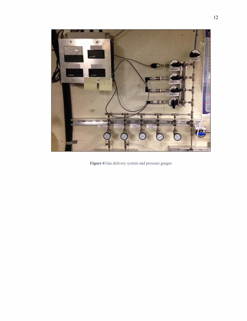
pictures up to 40,000 frames per second. The chamber is heated using two band heaters

attached on both ends of the cylindrical vessel which are capable of heating the chamber

upwards of 500 K because of the limits of O-rings and pressure transducer highlighted in

Figure 3. Pressure rise data during the combustion is determined through the use of a Kistler

603B1 pressure transducer connected to a Kistler 5010B charge amplifier which converts

the 4-20 mA signal from the transducer into a 10mV/PSIa signal which is relayed to the

analog to Digital conversion box in order to record the pressure data as a function of time

at the wall.

 

10  

 

Figure 2 Schematic of cylindrical chamber

 

Figure 3 Cylindrical chamber with two band heaters

 

 

 

11  

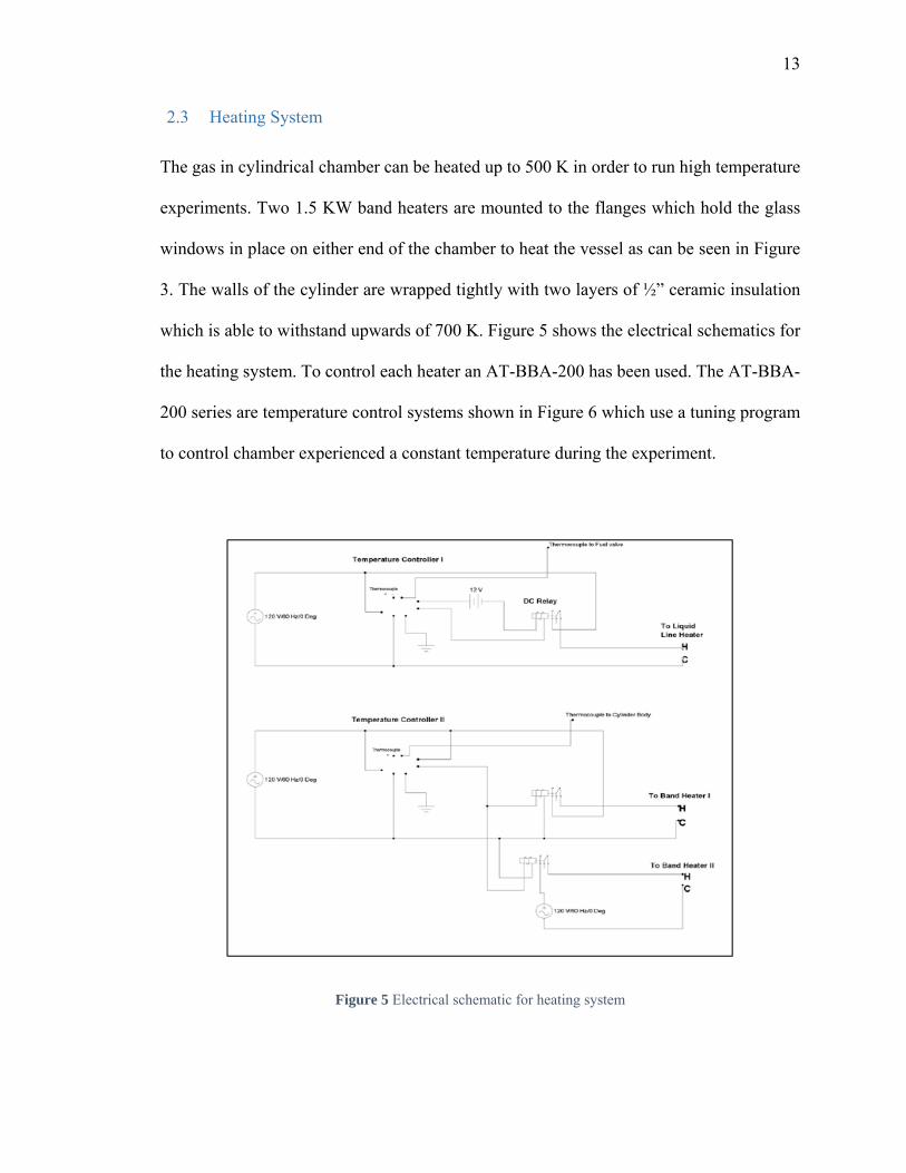
2.2 Gas Delivery System

The cylindrical chamber is connected to a gas delivery system shown in Figure 4. This

system consists of a valve manifold connected to gas tanks to distribute each component

of gas mixtures to the vessel by different pipes and a vacuum pump that is used to evacuate

the system. Four pressure gauges are used during the filling procedures. The first one has

a thermocouple pressure transducer which measures low vacuum levels and is used to

determine when the vessel is sufficiently evacuated (around 100 millitorr). The other three

equipped with piezoelectric pressure transducers and have different operation ranges; 0-15

psi, 0-30 psi, and 0-50 psi respectively. The pressure gauge which has the closest operation

range to the desired initial pressure of testing mixture is used to fill each component in the

chamber by the method of partial pressures. The vacuum pump is used to evacuate the

system not only between tests but between each individual component as well.

 

12  

 

Figure 4 Gas delivery system and pressure gauges

13  

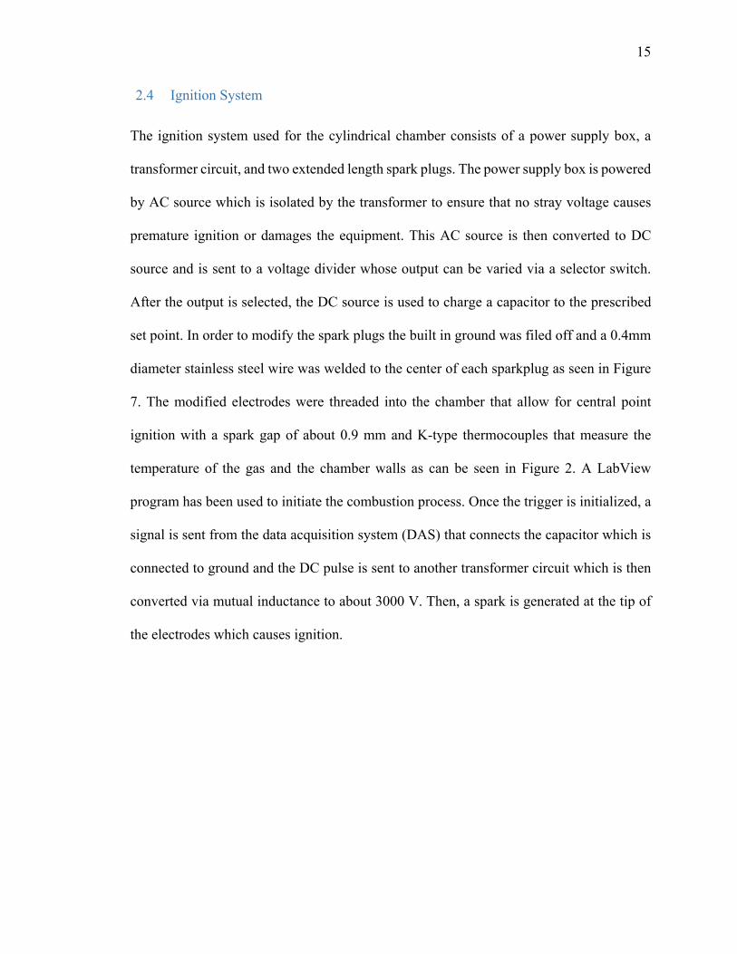
2.3 Heating System

The gas in cylindrical chamber can be heated up to 500 K in order to run high temperature

experiments. Two 1.5 KW band heaters are mounted to the flanges which hold the glass

windows in place on either end of the chamber to heat the vessel as can be seen in Figure

3. The walls of the cylinder are wrapped tightly with two layers of ½” ceramic insulation

which is able to withstand upwards of 700 K. Figure 5 shows the electrical schematics for

the heating system. To control each heater an AT-BBA-200 has been used. The AT-BBA-

200 series are temperature control systems shown in Figure 6 which use a tuning program

to control chamber experienced a constant temperature during the experiment.

 

 

Figure 5 Electrical schematic for heating system

 

14  

 

Figure 6 AT-BBA-200 PID controllers for band heaters

 

 

 

 

 

 

 

 

 

15  

2.4 Ignition System

The ignition system used for the cylindrical chamber consists of a power supply box, a

transformer circuit, and two extended length spark plugs. The power supply box is powered

by AC source which is isolated by the transformer to ensure that no stray voltage causes

premature ignition or damages the equipment. This AC source is then converted to DC

source and is sent to a voltage divider whose output can be varied via a selector switch.

After the output is selected, the DC source is used to charge a capacitor to the prescribed

set point. In order to modify the spark plugs the built in ground was filed off and a 0.4mm

diameter stainless steel wire was welded to the center of each sparkplug as seen in Figure

7. The modified electrodes were threaded into the chamber that allow for central point

ignition with a spark gap of about 0.9 mm and K-type thermocouples that measure the

temperature of the gas and the chamber walls as can be seen in Figure 2. A LabView

program has been used to initiate the combustion process. Once the trigger is initialized, a

signal is sent from the data acquisition system (DAS) that connects the capacitor which is

connected to ground and the DC pulse is sent to another transformer circuit which is then

converted via mutual inductance to about 3000 V. Then, a spark is generated at the tip of

the electrodes which causes ignition.

 

16  

 

Figure 7 Extended length spark plugs

 

 

 

 

 

 

 

17  

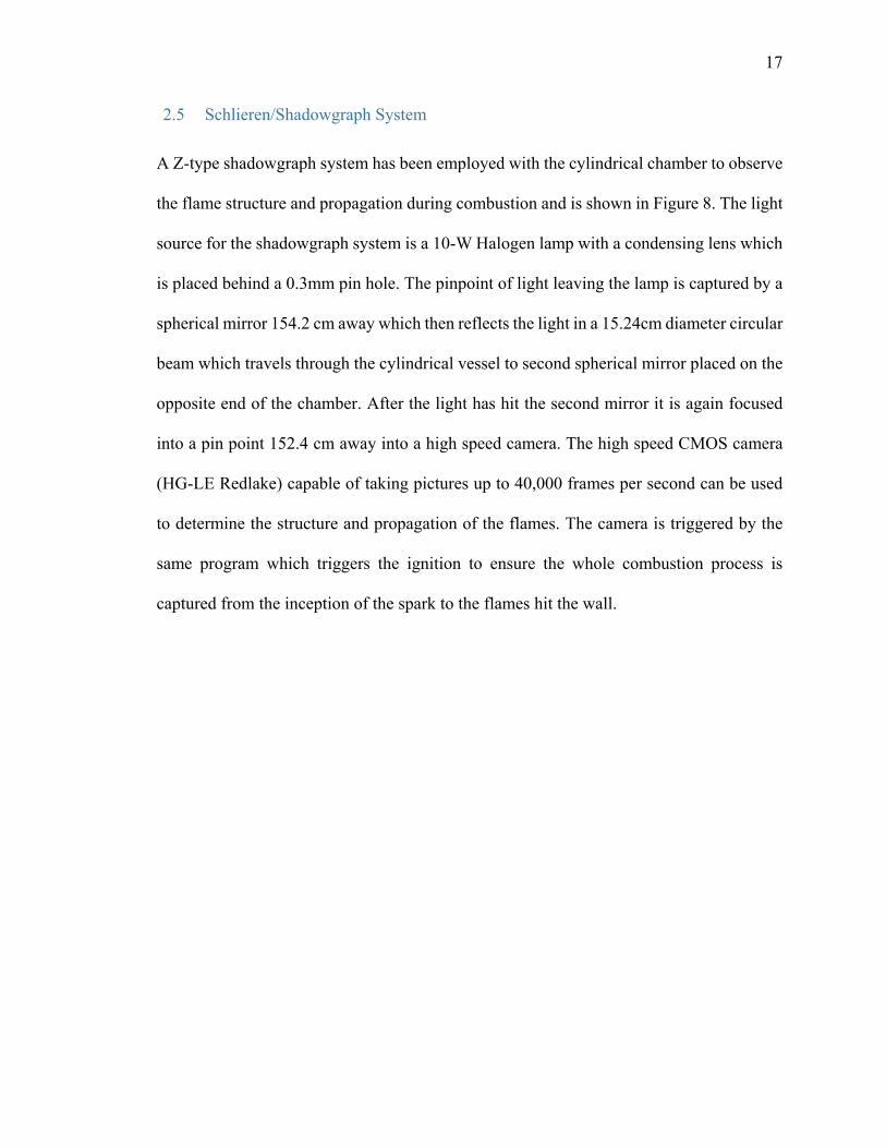
2.5 Schlieren/Shadowgraph System

A Z-type shadowgraph system has been employed with the cylindrical chamber to observe

the flame structure and propagation during combustion and is shown in Figure 8. The light

source for the shadowgraph system is a 10-W Halogen lamp with a condensing lens which

is placed behind a 0.3mm pin hole. The pinpoint of light leaving the lamp is captured by a

spherical mirror 154.2 cm away which then reflects the light in a 15.24cm diameter circular

beam which travels through the cylindrical vessel to second spherical mirror placed on the

opposite end of the chamber. After the light has hit the second mirror it is again focused

into a pin point 152.4 cm away into a high speed camera. The high speed CMOS camera

(HG-LE Redlake) capable of taking pictures up to 40,000 frames per second can be used

to determine the structure and propagation of the flames. The camera is triggered by the

same program which triggers the ignition to ensure the whole combustion process is

captured from the inception of the spark to the flames hit the wall.

18  

 

 

Figure 8 A Z-type Schlieren/Shadowgraph system

19  

2.6 Experimental Procedure

At first, the initial conditions should be found in a spreadsheet named “test matrix excel

sheet”. To begin testing, the combustion chamber and gas lines must be evacuated to a

sufficiently low pressure (around 100 millitorr) by using the vacuum pump. After the low

pressure has been achieved the gas delivery system is then used to fill hydrogen, carbon

monoxide, and helium/oxygen in the chamber to their desired pressures. The pressure of

each specific component is determined by the method of partial pressures through the use

of a spreadsheet that takes into account variables such as the pressure transducers zero

offset, the equivalence ratio, initial pressure, and percentage of hydrogen. The gases are

filled by order of ascending partial pressures which changes depending on the tests initial

conditions. The first component is filled using the gas manifold, once the desired pressure

of the first gas is reached, then the valve to the cylindrical vessel is closed and the lines

within the manifold system should be again evacuated to sufficiently low pressure. The

valve for the second component of the mixture is opened and once the pressure in the line

have already exceeded twice the pressure of the previous component of the mixture in the

chamber, the valve to the vessel is reopened allowing for the second mixture to flow into

the chamber without experiencing any backflow, improving overall accuracy. This process

is repeated for the number of components present in the combustible mixture. In the present

testing, there are three components in total. Once the chamber has been filled, the mixture

is left to wait for several minutes, which allows the mixture to become quiescent that

prevents turbulence within the vessel and allows the mixture to become homogenous.

Laminar burning speed measurements were restricted to flames with radii larger than 4 cm,

where the effects of stretch can be neglected. Measurements can only be employed for

20  

when the flame has radii larger than 4 cm and prior to when it reaches the inner wall of the

chamber or when it starts to be cellular, during which time the pressure method can be used

to calculate the laminar burning speed. The high speed camera and shadowgraph system

are used to study flame symmetry, stability, and structure during each test.

 

 

   

21  

3 Burning Speed Model

The model employed to calculate the laminar burning speed based on the pressure rise

inside the combustion chamber is based on one previously developed by Metghalchi and

Keck [33] and co-workers [34-35] that has since been modified to include several

correction factors for energy loss to the spark electrodes, radiative energy loss to the

chamber walls as well as the temperature gradient in the preheat zone by Eisazadeh-Far et

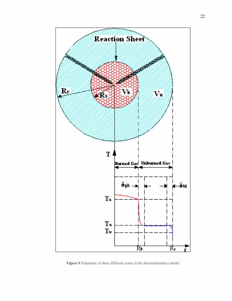
al [18]. It is assumed that gases in the combustion chamber can be divided into burned and

unburned regions separated by a reaction layer of zero thickness as shown in Figure 9

schematically. The burned gas inside the reaction layer is divided into ‘n’ number of shells

where ‘n’ is directly proportional to the duration of the combustion event. Each shell has a

distinct independent temperature that may differ from that of the surrounding shells, yet

the burned gas remains in chemical equilibrium. As shown in Figure 9, there exists a small

preheat zone of thickness δph which consists of unburned gas at a higher temperature than

the far field unburned gas due to energy transfer from the reaction layer beyond the reaction

layer. Core unburned gas with uniform temperature surrounds the preheat zone gases.

Beyond the preheat layer and unburned gas there exists a thermal boundary layer δbl which

separates the unburned gas from the wall. The effect of energy transfer from the unburned

to the spark electrodes is considered by a thermal boundary layer δbl same as the wall.

Further assumptions include that both the burned and unburned gases always behave as

ideal gases, both gases compress isentropically, the composition of the unburned gas is

constant, the pressure throughout the chamber is uniform, and the heat flux due to the

temperature gradient in the burned gas is negligible.

22  

 

Figure 9 Schematic of three different zones in the thermodynamics model

23  

3.1 Burned Gas Mass Fraction and Temperature

For spherical flames, the distribution of temperature in the burned and unburned gas region

and the burned gas mass fraction can be determined from the measured pressure using the

equations for mass and energy balance together with the ideal gas equation of state

                                                                  (2) 

In this equation, is the pressure which is measured within the chamber, is the specific

volume, is the specific gas constant, and is the temperature.

The mass balance equation for the burned and unburned gas region is

/                               (3) 

where is the total mass of the chamber, is the mass of the burned gas zone, is the

mass of the unburned gas zone, is the volume of the chamber and is the volume of the

spark electrodes. In this equation, the subscript denotes the initial conditions, and

subscripts and represent the burned gas and unburned conditions respectively. And

is the average density and is the volume of the gas.

The total volume of the gas in the combustion chamber is

                                                     (4) 

where

, ,                            (5)

is the volume of the burned gas, is the specific volume of isentropically compressed

burned gas,

                                                   (6) 

is the displacement volume of the electrode boundary layers,

24  

, 1                          (7) 

is the volume of the unburned gas, / is the burned gas mass fraction, is the

specific volume of the isentropically compressed unburned gas,

                                                   (8) 

is the displacement volume of the wall boundary layer, and

                                                   (9) 

is the displacement volume of the preheat zone ahead of the reaction layer.

The energy balance equation is

                                           (10) 

where is the initial energy of the gas, is the conductive energy loss to the electrodes,

is the energy loss to the wall, is the radiation energy loss,

, ,                          (11) 

is the energy of the burned gas, is the specific energy of isentropically compressed

burned gas,

(12)

is the energy defect of the electrode boundary layer,

, 1 (13)

is the energy of the unburned gas, is the specific energy of the isentropically

compressed unburned gas,

(14)

is the energy defect of the wall boundary, and

25  

(15)

is the energy defect of the preheat layer.

The definition of enthalpy

(16)

Using ideal gas assumption, constant specific heat

(17)

(18)

(19)

Combining Equation (17) with Equations (18) and (19), the following equation is

developed

/ 1 (20)

where is the enthalpy of formation of the gas at zero degrees Kelvin and is the specific

heat ratio. By this relation, Equations (12), (14), and (15) can be written as

(21)

/ 1 (22)

(23)

/ 1 (24)

(25)

/ 1 (26)

26  

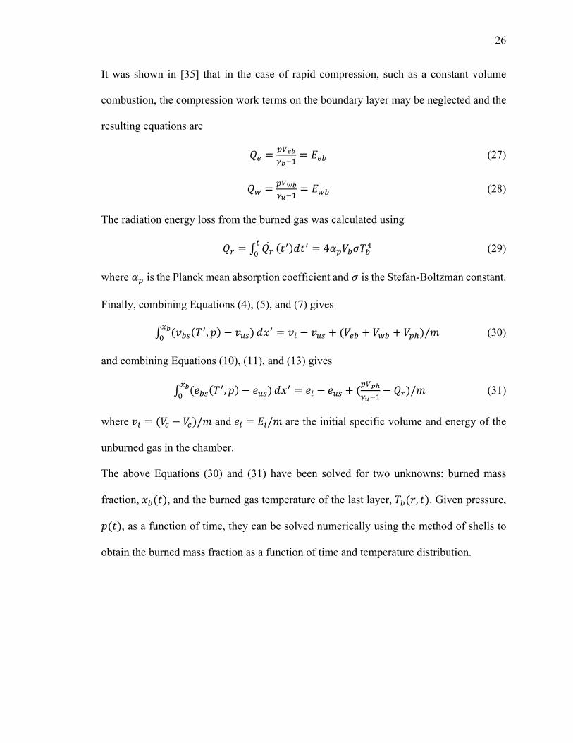
It was shown in [35] that in the case of rapid compression, such as a constant volume

combustion, the compression work terms on the boundary layer may be neglected and the

resulting equations are

(27)

(28)

The radiation energy loss from the burned gas was calculated using

4 (29)

where is the Planck mean absorption coefficient and is the Stefan-Boltzman constant.

Finally, combining Equations (4), (5), and (7) gives

, / (30)

and combining Equations (10), (11), and (13) gives

, / (31)

where / and / are the initial specific volume and energy of the

unburned gas in the chamber.

The above Equations (30) and (31) have been solved for two unknowns: burned mass

fraction, , and the burned gas temperature of the last layer, , . Given pressure,

, as a function of time, they can be solved numerically using the method of shells to

obtain the burned mass fraction as a function of time and temperature distribution.

27  

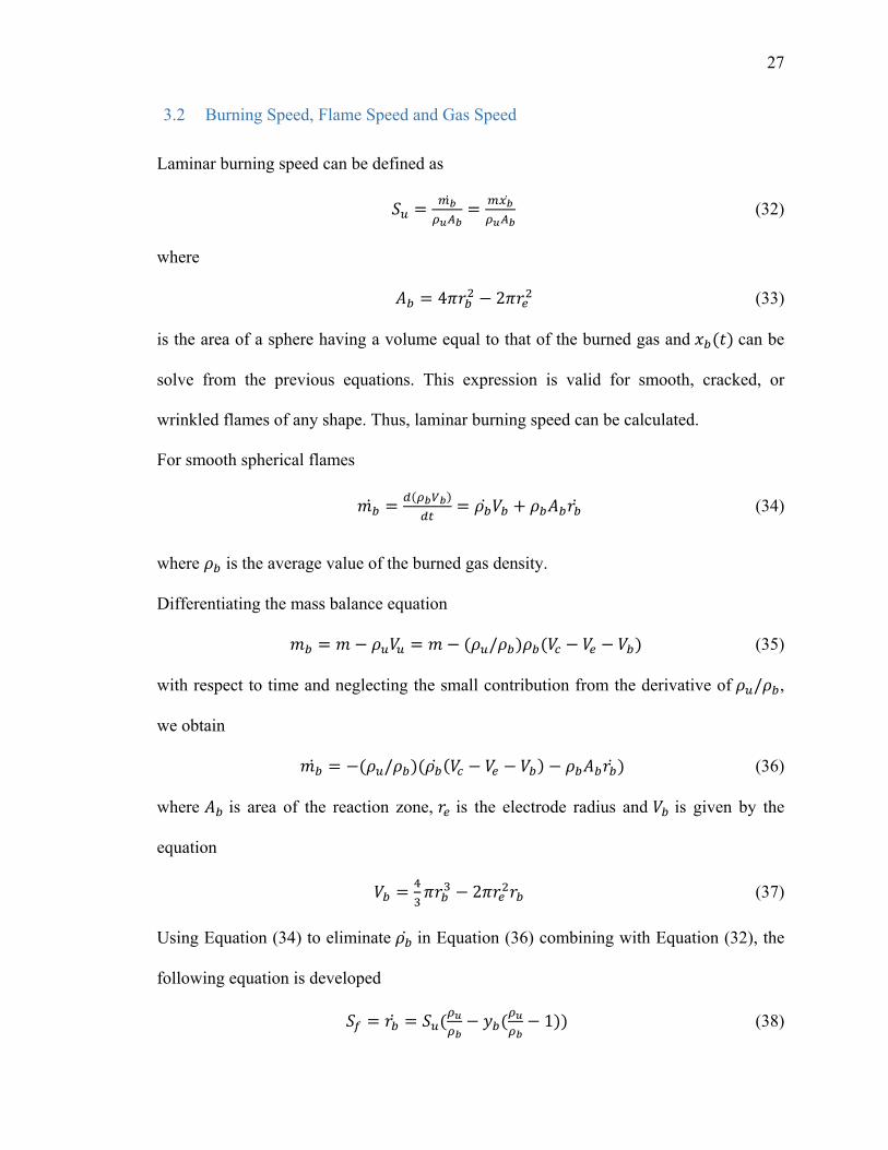
3.2 Burning Speed, Flame Speed and Gas Speed

Laminar burning speed can be defined as

(32)

where

4 2 (33)

is the area of a sphere having a volume equal to that of the burned gas and can be

solve from the previous equations. This expression is valid for smooth, cracked, or

wrinkled flames of any shape. Thus, laminar burning speed can be calculated.

For smooth spherical flames

                                            (34) 

where is the average value of the burned gas density.

Differentiating the mass balance equation

/ (35)

with respect to time and neglecting the small contribution from the derivative of / ,

we obtain

/ (36)

where is area of the reaction zone, is the electrode radius and is given by the

equation

2 (37)

Using Equation (34) to eliminate in Equation (36) combining with Equation (32), the

following equation is developed

1 (38)

28  

where is the flame speed and / is the burned gas volume fraction. Note

that for 0, / and for 1, .

The gas speed is defined as

(39)

Substituting Equation (38) into Equation (39) gives

1 1 (40)

This completes the equations for the burning model.

29  

4 Results and Discussion

In this section, the range of conditions tested, the flame structures, the methodology used

to process the data, and the laminar burning speed results in the present works are discussed.

Additionally, the topic of stretch along with its impact on the reported laminar burning

speed is discussed as well.

4.1 Range of Conditions Tested

Laminar burning speed and flame structure tests have been conducted for syngas that has

three different hydrogen concentrations (α = 5%, 10% and 25%) with oxygen/helium

mixture over a wide range of initial temperatures (Ti = 298 K, 400 K and 480 K), initial

pressures (Pi = 0.5 atm, 1 atm and 2 atm), and equivalence ratios ( = 0.6, 1, 2 and 3) which

are defined as /

/, where / is the mixture ratio of fuel to oxygen/helium,

and / is the ratio of fuel to oxygen/helium required for stoichiometric

combustion. Based on these initial conditions, laminar burning speed has been studied for

temperatures ranging from 298 K to 650 K, pressures between 0.5 to 7.3 atmospheres and

equivalence ratios ranging from 0.6 to 3.0. And the global reaction is

∗ 1 0.5 ∗ 3.77 → (38)

4.2 Flame Structure and Instability Study

The initiation and propagation of flame instability have been investigated in this section.

The transition from smooth flame to cellular flame is determined by inspection of the

images captured by the high speed camera during flame propagation. There are two

30  

significant instabilities named hydrodynamic instability and diffusive-thermal instability

always occur in premixed flames [31].

The hydrodynamic instability is due to the gas expansion that results from the energy

released by chemical reactions, which induces a flow that tends to make any flame

perturbation further away from the original shape. The growth rate of the hydrodynamic

disturbance is associated to the thermal expansion ratio which is defined as the ratio of

the density of unburned gas ( ) to the density of burned gas ( ) [36] and the flame

thickness which is defined as / / [37]. In present works, the

flames thickness increase by using helium instead of nitrogen so that the hydrodynamic

instability decrease, the flames become smoother.

The diffusive-thermal instability is due to the disparity of thermal diffusion from the flame

and mass diffusion towards the flame [38-40]. The convex parts of flame surface convent

more energy because they are toward to the unburned mixture which has low temperature.

As a result, the temperature of these parts decrease due to thermal diffusion, which slows

down the forward speed of the convex parts. On the contrary, the concave parts convent

less energy so that the temperature as well as the forward speed increase. Thus, the surface

of the flame front is smoothed out.

However, mass diffusion has the opposite effect. The convex parts of flame surface receive

more fuel because they are toward to the unburned mixture. The reaction rate and the

temperature increase in the convex parts of the flame front which result in a greater front

curvature. But, the concave parts receive less fuel so that the reaction rate as well as the

temperature decrease in the concave parts of the flame front which also result in a greater

front curvature. If the mass diffusivity of the reactant is sufficiently greater than the

31  

thermal diffusivity of the mixture, we can expect a flame front to be unstable due to

the diffusive-thermal effect, in the opposite case, the flame front should be stable [39]. In

present works, because helium has a greater thermal diffusivity than nitrogen, the diffusive-

thermal instability decrease, the flames become smoother.

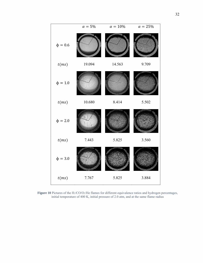
It can be seen in Figure 10, the effects of hydrogen percentage of syngas and equivalence

ratio on the instability of the flame front have been examined. With the increasing of

hydrogen from 5% to 25% in the fuel, the flame becomes much more sensitive to instability.

That is because the reduction of flame thickness and Lewis number, which are the factors

of hydrodynamic instability and diffusive-thermal instability. When the equivalence ratio

increases from 0.6 to 3.0, the flame instability increases as well.

Figure 11 shows the hydrodynamic effects, due to the decrease of the flame thickness, play

a significant role on flame instability as initial pressure increases from 0.5 atm to 2.0 atm.

Hydrodynamic instability decreases due to the increase of the flame thickness as initial

temperature increases from 298 K to 480 K.

Figure 12 presents, substituting nitrogen with helium makes the flame much more stable

and smooth at same conditions due to the increase of flame thickness and Lewis number

that decreases diffusive-thermal and hydrodynamic instabilities.

 

 

 

 

 

32  

5% 10% 25%

ɸ 0.6

19.094 14.563 9.709

ɸ 1.0

10.680 8.414 5.502

ɸ 2.0

7.443 5.825 3.560

ɸ 3.0

7.767 5.825 3.884

Figure 10 Pictures of the H2/CO/O2/He flames for different equivalence ratios and hydrogen percentages, initial temperature of 400 K, initial pressure of 2.0 atm, and at the same flame radius

 

 

 

33  

0.5 1.0 2.0

298

5.178 4.531 3.884

400

4.531 3.560 3.560

480

3.884 3.884 3.236

Figure 11 Pictures of the H2/CO/O2/He flames for different pressures and temperatures, hydrogen percentage of 25%, equivalence ratio at 2.0, and at the same flame radius

 

 

 

 

 

 

34  

O2+N2 O2+He

5%

28.479 11.974

10%

20.388 9.062

25%

12.298 5.825

Figure 12 Pictures of the H2/CO/O2/diluent flames for different diluents of nitrogen and helium, initial temperature 298 K, initial pressure 2.0 atm, equivalence ratio 1.0, and at the same radius

 

 

 

 

 

35  

4.3 Stretch effect investigation

Laminar burning speed of stretched flames is different from that of zero stretch flames.

Zero stretch laminar burning speeds in many experiments are always estimated by

extrapolating the stretched burning speed data to zero stretch by various linear and

nonlinear models. Flame stretch in propagating spherical flame is defined as

(39)

where is the stretch rate, is the area of flame, is time, and is the radius of the flame.

Equation (39) shows that the stretch rate decreases as the flame radius increases. In order

to study the effects of stretch, laminar burning speeds have been measured at same

unburned gas properties and radii greater than 4 cm with different stretch rates. A series of

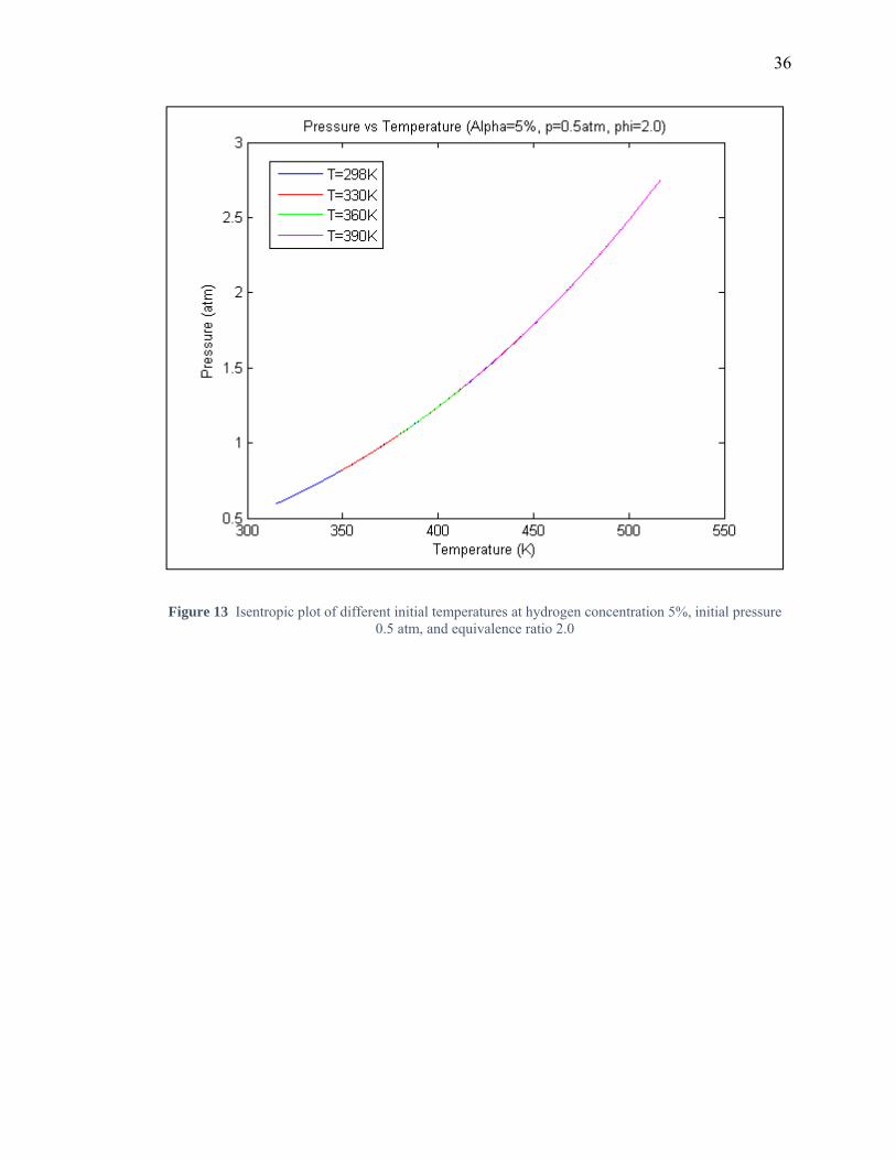
tests at Ti = 298 K, 330 K, 360 K, and 390 K were conducted at equivalence ratios of 2.0

and pressures corresponding to the specific isentropic process Figure 13. By conducting

several different experiments along the same isentropic line, the laminar burning speed can

be determined for the same pressure, temperature and equivalence ratio with different

stretch rates due to different flame radii. Figure 14 shows the variation of laminar burning

speed versus stretch for unburned gas conditions. In Figures 14, the horizontal line is the

average laminar burning speed plotted against the stretch rate. It can illustrate that the

laminar burning speeds do not change for flame radii greater than 4 cm [41-43]. Because

laminar burning speed of syngas/oxygen/helium is greater than syngas/air, the stretch rates

for large radii are between 100 to 280 1/s. In this thesis, the laminar burning speed results

are only for smooth flames with radii greater than 4 cm.

 

   

36  

 

Figure 13 Isentropic plot of different initial temperatures at hydrogen concentration 5%, initial pressure 0.5 atm, and equivalence ratio 2.0

 

   

37  

 

Figure 14 Laminar burning speed of different initial temperatures (stretch rates) at hydrogen concentration 5%, initial pressure 0.5 atm, and equivalence ratio 2.0

 

   

38  

4.4 Data Processing

Laminar burning speed calculations were limited to smooth flames with radii greater than

4 cm where the effects of stretch become negligible as discussed in previous section. Thus,

the pressure rise data of the beginning of combustion event before the flame radius larger

than 4 cm as well as the pressure data that was obtained after the flame become unstable

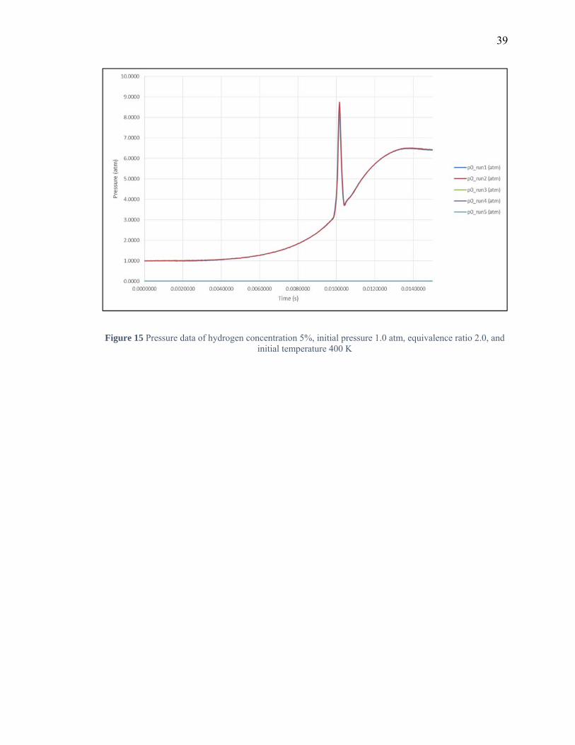
or it reaches the wall were removed. A method for determining when the flame hits the

wall is by observing the pressure time plots, an example is shown as Figure 15. In this plot,

there is a large spike in pressure data result from the flame has reached the wall, thus all

data after the pressure starts to rapidly increase must be discarded. Another method to

determine this point is by using the high speed camera and analyzing the flame propagation

on a frame by frame basis. Besides, when the flames become cellular before the flames hit

the wall, the pressure data of cellular flame were discard as well. The cellularity of the

flame can be defined by high speed camera as discussed in section 4.2. At the beginning

of the stage, the pressure data is not smoothed due to signal noise generated by high sample

frequency (15 KHz). In order to prevent the burning speed code from crashing, the pressure

data should be smoothed so that it reflects the physics of the combustion event. The

smoothed data can be used as the input of thermodynamic code which can calculator the

laminar burning speed and other properties.

 

   

39  

 

Figure 15 Pressure data of hydrogen concentration 5%, initial pressure 1.0 atm, equivalence ratio 2.0, and initial temperature 400 K

 

 

 

 

 

 

 

 

 

40  

4.5 Laminar Burning Speed

Experiments were conducted for the conditions listed in section 4.1 and the pressure time

data from these experiments were fed into the thermodynamic code discussed in section 3

and 4.4. The laminar burning speed results generated by the thermodynamic code are

presented in Figures 16 through 22.

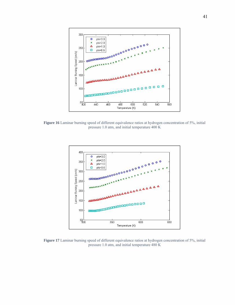
Figure 16 and 17 present the laminar burning speed for Ti = 400 K and 480 K, Pi = 1.0, α

= 5% and all tested equivalence ratios. From this graph, it is clear that the leanest mixture

has the lowest laminar burning speed and the richest mixture has the highest laminar

burning speed. As the equivalence ratio increases from 0.6 to 3.0, there is a rapid increase

in laminar burning speed.

Figure 18 and 19 present the laminar burning speed for Ti = 400 K and 480 K, Pi = 1.0, phi

= 1.0 for different hydrogen concentrations in the fuel. From this graph, it is clear that the

smallest hydrogen concentration has the lowest laminar burning speed and the largest

hydrogen concentration has highest laminar burning speed. As the hydrogen concentration

increases from 5% to 25%, there is a rapid increase in laminar burning speed.

Figure 20 and 21 present the laminar burning speed for Ti = 298 K and 400 K, phi = 0.6, α

= 25% and all tested initial pressures. From this graph, it is clear that the lowest initial

pressure has the highest laminar burning speed and the highest initial pressure has the

lowest laminar burning speed. As the initial pressure increase from 0.5 to 2.0, there is a

rapid decrease in laminar burning speed.

Figure 22 presents the laminar burning speed for the initial condition Ti = 298 K, Pi = 1.0,

phi = 0.6, α = 5% of air and helium oxygen mixture. From the graph, it is clear that the

laminar burning speed increase by using helium instead of nitrogen.

41  

 

Figure 16 Laminar burning speed of different equivalence ratios at hydrogen concentration of 5%, initial pressure 1.0 atm, and initial temperature 400 K

 

Figure 17 Laminar burning speed of different equivalence ratios at hydrogen concentration of 5%, initial pressure 1.0 atm, and initial temperature 480 K

 

   

42  

 

Figure 18 Laminar burning speed of different hydrogen concentrations at initial pressure 1.0 atm, equivalence ratio 1.0, and initial temperature 400 K

 

Figure 19 Laminar burning speed of different hydrogen concentrations at initial pressure 1.0 atm, equivalence ratio 1.0, and initial temperature 480 K

 

   

43  

 

Figure 20 Laminar burning speed of different initial pressures at hydrogen concentration 25%, equivalence ratio 0.6, and initial temperature 298 K

 

Figure 21 Laminar burning speed of different initial pressures at hydrogen concentration 25%, equivalence ratio 0.6, and initial temperature 400 K

 

   

44  

 

Figure 22 Laminar burning speed of different diluents at hydrogen concentration 5%, initial pressure 1.0 atm, equivalence ratio 1.0, and initial temperature 298 K

 

   

45  

5 Conclusions

The laminar burning speed and flame instability of spherically expanding flames of syngas

that has three different hydrogen concentrations (5%, 10% and 25%) oxygen and helium

mixture have been studied over a wide range of equivalence ratios (0.6, 1, 2 and 3), initial

mixture temperatures (298 K, 400 K and 480 K) and initial pressures (0.5atm, 1atm and

2atm) by the pressure rise data during spherical flame propagations. Laminar burning speed

measurements covered a wide range of temperatures and pressures up to 650 K and 7.3

atm. As the equivalence ratio increase from 0.6 to 3.0, laminar burning speed of this

mixture increases. And it also increases with increasing hydrogen concentration in the fuel.

With the hydrogen percentage increasing, the flame become more cellular at lower

equivalence ratios. The laminar burning speeds of H2/CO/O2/He flames decrease as the

pressures increase. Besides, when the initial pressures increase, the instabilities of flames

take place earlier due to hydrodynamic effects. Comparing helium with nitrogen, the flame

of helium mixture is much more stable than nitrogen, and also, the laminar burning speed

of helium mixture is faster than that of nitrogen.

46  

REFERENCE

1. Keck, J. C. (1982). Turbulent Flame Structure and Speed in Spark Ignition Engines,

Nineteenth International Symposium on Combustion. 1451-1466.

2. Ferguson, C. R. and Keck, J. C. (1977). On Laminar Flame Quenching and Its

Application to Spark Ignition Engines, Combustion and Flame. 28, 197-205.

3. Frenklach, M. (1991). Reduction of Chemical Reaction Models, Numerical

Approaches to Combustion Modeling, Progress in Astronautics and Aeronautics.

135, Chapter 5, 129-150.

4. Turns, S.R. (2000). An Introduction to Combustion. Boston: McGraw Hill. 1, 1-8.

5. EPA. (2010, August 19). The Montreal Protocol on Substances that Deplete the

Ozone Layer. August 2011: http://www.epa.gov/ozone/intpol/.

6. Linnett, J. W. (1953). Methods of Measuring Burning Velocities, Fourth

Symposium (International) on Combustion. Baltimore: Williams and Wilkins.

7. Andrews, G. E. and Bradley D. (1972). Determination of Burning Velocities: A

Critical Review, Combustion and Flame. 18, 133-153.

8. Rallis C. J. and Garforth A. M., Determination of Laminar Burning Velocity,

Progress in Energy and Combustion Science, 6 (1980) 303-329.

9. Van Maaren, A, Thung, D.S., De Goey, L.P.H. (1994). Measurement of Flame

Temperature and Adiabatic Burning Velocity of Methane/Air Mixtures. Combust.

Sci. and Tech. 96, 327-344.

47  

10. Wu, C.K., Law, C.K. (1985). On The Determination of Laminar Flame Speeds from

Stretched Flames. The Combustion Institute. 1941-1949

11. Tsuji, H. (1982). Counterflow diffusion flames. Prog. Energy and Combust. Sci. 8,

93-119.

12. Egolfopoulos, F.N., Cho, P., Law, C.K. (1989). Laminar flame speeds of methane

air mixtures under reduced and elevated pressures. Combustion and Flame. 76,

375-391.

13. Apurba K. Das, Kamal Kumar, Chih-Jen Sung. (2011). Laminar flame speeds of

moist syngas mixtures. Combustion and Flame. 158, 345-353.

14. Mallard, E., Le Chatelier, H. L. (1883). Ann. Mines, Sec. IV 8, 274.

15. Mikhel’son, V. A. (1892). Quoted in Physics of Combustion and Explosion (L. N.

Khitrin) Israel program for Scientific Translations, Jerusalem (1962), 138-140.

16. Coward, H. F., Hartwell, F. J. (1932). J. Chem. Soc., 2676.

17. Coward, H. F., Payman, W. (1937). Chem. Rev., 21, 359.

18. Eisazadeh-Far, K., Parsinejad, F., Metghalchi, H. (2010). Flame structure and

laminar burning speeds of JP-8/air premixed mixtures at high temperatures and

pressures. Fuel. 89, 1041-1049.

19. McLean, I. C., Smith, D. B., & Taylor, S. C. (1994). The Use of Carbon

Monoxide/Hydrogen Burning Velocities to Examine the Rate of the CO + OH

Reaction. Symp. (Int.) Combust.25, 749-757.

20. Hassan, M. I., Aung, K. T., & Faeth, G. M. (1997). Properties of laminar premixed

CO/H2/air flames at various pressures. J. Propuls. Power. 13, 239-245

48  

21. Qin, X., & Ju, Y. (2005). Measurements of burning velocities of dimethyl ether and

air premixed flames at elevated pressures. Proc. Combust. Inst. 30, 233-240.

22. Takizawa, K., Takahashi, A., Tokuhashi, K., Kondo, S., Sekiya A. (2005). Burning

velocity measurement of fluorinated compounds by the spherical-vessel method.

Combustion and Flame. 141, 298-307.

23. Lewis, B., von Elbe, G. (1961). Combustion, Flames, and Explosion of gases, 2nd

edition, Academic Press.

24. Metghalchi, H., Keck, J.C. (1980). Laminar Burning Velocity of Propane-Air

Mixtures at High Temperature and Pressure. Combustion and Flame. 38, 143-154.

25. Sun, H., Yang, S. I., Jomaas, G., and Law, C. K. (2007). High-pressure laminar

flame speeds and kinetic modeling of carbon monoxide/hydrogen combustion 31,

439-446.

26. Som, S., Ramírez, a. I., Hagerdorn, J., Saveliev, a., and Aggarwal, S. K. (2008). A

numerical and experimental study of counter flow syngas flames at different

pressures Fuel. 87, 319-334.

27. Natarajan, J., Kochar, Y., Lieuwen, T., and Seitzman, J. (2009). Pressure and

preheat dependence of laminar flame speeds of H2/CO/CO2/O2/He mixtures. Proc.

Combust. Inst. 32, 1261-1268.

28. Park J, Lee D. H., Yoon S. H., Vu T. M., Yun J. H., Keel S. I. (2009). Effects of

Lewis number and preferential diffusion on flame characteristics in

80%H2/20%CO syngas counterflow diffusion flames diluted with He and Ar.

International Journal of Hydrogen Energy. 34, 1578-84.

49  

29. M. P. Burke, M. Chaos, F. L. Dryer, Y. Ju. (2010). Negative pressure dependence

of mass burning rates of H2/CO/O2/diluent flames at low flame temperatures.

Combust. Flame. 157, 618-631.

30. T. M. Vu, J. Park, O. B. Kwon, D. S. Bae, J. H. Yun, S. I. Keel. (2010). Effects of

diluents on cellular instabilities in outwardly propagating spherical syngas-air

premixed flames. Int. J. Hydrogen Energy. 35, 3868-3880.

31. Qiao L, Kim C. H., Faeth G. M.. (2005). Suppression effects of diluents on laminar

premixed hydrogen/oxygen/nitrogen flames. Combustion and Flame 143. 79-96.

32. S. D. Tse, D. L. Zhu and C. K. Law. (2000). Morphology and Burning Rates of

Expanding Spherical Flames in H2/O2/Inert Mixtures Up To 60 Atmospheres.

Proceedings of the Combustion Institute. 28, 1793-1800.

33. Metghalchi, M., Keck, J. C. (1982). Burning velocities of mixtures of air with

methanol, isooctane, and indolene at high pressure and temperature. Combust

Flame. 48, 191-210.

34. Rahim F, Eisazadeh Far K, Parsinejad F, Andrews RJ, Metghalchi H. (2008). A

thermodynamic model to calculate burning speed of methane–air-diluent mixtures.

Int J Thermodyn. 11, 151-61.

35. Parsinejad F, Arcari C, Metghalchi H. (2006). Flame structure and burning speed

of JP-10 air mixtures. Combust Sci Technol. 178, 975-1000.

36. Kadowaki, S., Suzuki, H., Kobayashi, H., and Im, H. G. (2005). The unstable

behavior of cellular premixed flames induced by intrinsic instability. Proceedings

of the Combustion Institute. 30, 169-176.

50  

37. Law, C. K., and Kwon, O. C. (2004). Effects of hydrocarbon substitution on

atmospheric hydrogen-air flame propagation. International Journal of Hydrogen

Energy. 29, 867-879.

38. Sivashinsky G.I. (1977). Diffusional-thermal theory of cellular flames. Combust.

Sci. Technol. 15, 137-146.

39. Sivashinsky G.I. (1983). Instabilities, pattern formation, and turbulence in flames.

Annual Review of Fluid Mechanics. 15, 179-199.

40. Bechtold J.K, Matalon M. (1987). Hydrodynamic and diffusion effects on the

stability of spherically expanding flames. Combustion and Flame. 67, 77-90.

41. Eisazadeh-Far, K., Moghaddas, A., Al-Mulki, J., and Metghalchi, H. (2011). Laminar

burning speeds of ethanol/air/diluent mixtures. Proceedings of the Combustion

Institute. 33, 1021-1027.

42. Eisazadeh-Far, K., Moghaddas, A., Al-Mulki, J., Metghalchi, H., and Keck, J. C.

(2011). The effect of diluent on flame structure and laminar burning speeds of JP-

8/oxidizer/diluent premixed flames. Fuel. 90, 1476-1486.

43. Moghaddas, A., Eisazadeh-Far, K., and Metghalchi, H. (2012). Laminar burning

speed measurement of premixed n-decane/air mixtures using spherically expanding

flames at high temperatures and pressures. Combustion and Flame. 159, 1437-

1443.