MEASUREMENT OF BRUSHLESS DC MOTOR CHARACTERISTICS...

MEASUREMENT OF BRUSHLESS DC MOTOR CHARACTERISTICS AND PARAMETERS AND BRUSHLESS DC MOTOR DESIGN

A THESIS SUBMITTED TO THE GRADUATE SCHOOL OF NATURAL AND APPLIED SCIENCES

OF MIDDLE EAST TECHNICAL UNIVERSITY

BY

ĐLKER ŞAHĐN

IN PARTIAL FULFILLMENT OF THE REQUIREMENTS FOR

THE DEGREE OF MASTER OF SCIENCE IN

ELECTRICAL AND ELECTRONICS ENGINEERING

JANUARY 2010

Approval of the thesis:

MEASUREMENT OF BRUSHLESS DC MOTOR CHARACTERISTICS AND

PARAMETERS AND BRUSHLESS DC MOTOR DESIGN

submitted by ĐLKER ŞAHĐN in partial fulfilment of the requirements for the degree of Master of Science in Electrical and Electronics Engineering Department, Middle East Technical University by,

Prof. Dr. Canan ÖZGEN Dean, Graduate School of Natural and Applied Sciences _____________ Prof. Dr. Đsmet ERKMEN Head of Department, Electrical and Electronics Engineering _____________ Prof. Dr. H. Bülent ERTAN Supervisor, Electrical and Electronics Engineering Dept, METU _____________ Examining Committee Members: Prof. Dr. Muammer ERMĐŞ Electrical and Electronics Engineering Dept., METU _____________ Prof. Dr. H. Bülent ERTAN Electrical and Electronics Engineering Dept., METU _____________ Prof. Dr. Kemal LEBLEBĐCĐOĞLU Electrical and Electronics Engineering Dept., METU _____________ Prof. Dr. Aydın ERSAK Electrical and Electronics Engineering Dept., METU _____________ Bülent BĐLGĐN, M.Sc. ASELSAN Inc. _____________

Date: 10.12.2009

iii

I hereby declare that all information in this document has been obtained and

presented in accordance with academic rules and ethical conduct. I also declare

that, as required by these rules and conduct, I have fully cited and referenced all

material and results that are not original to this work.

Name, Last Name :

Signature :

iv

ABSTRACT

MEASUREMENT OF BRUSHLESS DC MOTOR CHARACTERISTICS AND PARAMETERS AND BRUSHLESS DC MOTOR DESIGN

Şahin, Đlker

M.Sc., Department of Electrical and Electronics Engineering

Supervisor: Prof. Dr. H. Bülent ERTAN

January 2010, 203 pages

The permanent magnet motors have become essential parts of modern motor drives

recently because need for high efficiency and accurate dynamic performance arose in the

industry. Some of the advantages they possess over other types of electric motors include

higher torque density, higher efficiency due to absence of losses caused by field excitation,

almost unity power factor, and almost maintenance free construction. With increasing need

for specialized PM motors for different purposes and areas, much effort has also gone to

design methodologies.

In this thesis a design model is developed for surface PM motors. This model is used with

an available optimization algorithm for the optimized design of a PM motor. Special

attention is paid to measurement of parameters of a sample PM motor.

As a result of this study, an effective analytical model with a proven accuracy by

measurement results is developed and applied in a design process of a surface PM motor.

Parametric and performance results of analytical model and tests have been presented

comparatively. A prototype motor has been realized and tested.

Keywords: permanent magnet motors, brushless dc, surface magnet motors, design

optimization, measurement of motor parameters, determination of motor parameters

v

ÖZ

FIRÇASIZ DC MOTOR KARAKTERĐSTĐĞĐ VE PARAMETRE ÖLÇÜMÜ VE

FIRÇASIZ DC MOTOR TASARIMI

Şahin, Đlker

Yüksek Lisans, Elektrik ve Elektronik Mühendisliği Bölümü

Tez Yöneticisi: Prof. Dr. H. Bülent ERTAN

Ocak 2010, 203 sayfa

Sabit mıknatıslı (SM) motorlar, sanayide ortaya çıkan yüksek verim ve dinamik performans

ihtiyaçlarından dolayı, modern motor sürücülerin temel parçalarından biri olmuştur. Diğer

motor türlerine nazaran öne çıkan bazı özellikleri daha yüksek moment yoğunluğu, alan akısı

uyartımının olmaması sayesinde daha yüksek verim, neredeyse birim güç faktörü ve bakım

gerektirmeyen yapısıdır. Değişik amaçlar ve uygulama alanlarına yönelik özel amaçlı SM

motorlar için artan ihtiyaç sebebiyle, tasarım yöntemlerine yönelik ayrıca gayret sarf

edilmektedir.

Bu tez çalışmasında, SM motorlar için bir tasarım modeli geliştirilmiştir. Halihazırdaki bir

optimizasyon algoritması ile bu model, bir SM motorun en iyileştirilmiş tasarımında

kullanılmıştır. Model parametrelerin ölçüm yöntemlerine özel çaba harcanmıştır.

Bu tez çalışmasının sonucu olarak, doğruluğu deneysel sonuçlarla kanıtlanmış bir tasarım

modeli geliştirilmiş ve bir SM motorun tasarımında kullanılmıştır. Analitik ve deneysel olarak

elde edilen model değişkenlerinin değerleri ve motor performans sonuçları karşılaştırmalı

olarak sunulmuştur. Prototip bir motor üretilmiş ve test edilmiştir.

Anahtar Kelimeler: sabit mıknatıslı motorlar, fırçasız dc, yüzey mıknatıslı motorlar, tasarım

optimizasyonu, motor parametrelerinin ölçülmesi, motor parametrelerinin belirlenmesi

vi

ACKNOWLEDGEMENTS

I would like to thank my advisor, Prof. Dr. H. Bülent Ertan, for all his support, expert

guidance and discussions about every aspect of my work.

I am grateful to people in Aselsan Inc. who initiated this work as a project and supported in

all phases; S. Yıldırım, B. Bilgin, Ü. Bülbül, B.T. Ertuğrul, M. Karataş, B. Gürcan, F.

Fenercioğlu.

I also wish to express my gratitude to U. Genç and E. Meşe in AVL Turkey for their

tolerance to my efforts for the this work during company time.

I can not forget my friends in the department office O. Keysan, V. Sezgin, B. Çolak,

K. Yılmaz, Đ. Mahariq, E. Doğru; my former house mates Z. Cansev, Đ. Yücel; musician

friends H. Altunbaşlıer, B. Yapıcı, C. Tuncer, M. Demireriden, S.C. Zor; and all others

including K. Kapucu, S. Özcan, S. Aldemir, S. Tunçağıl, E. Usta. Time would pass tediously

without them.

Finally, I would like to express my deepest love and gratitude to my parents Recep and

Raziye Şahin and my sister Ayşe Ezgi. I owe all my success to their great orientation and

support through my life. They are the ones who motivated me at all stages of academic

study. I dedicate my work to them.

İlker Şahin

Ankara, January 2010

vii

TABLE OF CONTENTS

ABSTRACT....................................................................................................................................... IV

ÖZ........................................................................................................................................................ V

ACKNOWLEDGEMENTS..............................................................................................................VI

TABLE OF CONTENTS................................................................................................................ VII

LIST OF TABLES ............................................................................................................................XI

LIST OF FIGURES .......................................................................................................................XIII

CHAPTER 1 INTRODUCTION ....................................................................................................... 1

1.1 PERMANENT MAGNETS .......................................................................................................... 6

1.2 CONCLUSION TO CHAPTER 1............................................................................................... 9

CHAPTER 2 BRUSHLESS DC MOTOR MODEL....................................................................... 11

2.1 MAGNETIC CIRCUIT ANALYSIS ON OPEN CIRCUIT ............................................................... 12

2.2 ELECTRIC CIRCUIT ANALYSIS .............................................................................................. 15

2.3 INDUCED EMF VOLTAGE ON OPEN CIRCUIT........................................................................ 18

2.4 STEADY STATE OPERATION .................................................................................................. 20

2.5 CONCLUSION TO CHAPTER 2............................................................................................. 21

CHAPTER 3 MEASUREMENT OF PERFORMANCE AND PARAMETERS OF

BRUSHLESS DC MACHINES........................................................................................................ 22

3.1 TEST MOTOR AND LABORATORY TEST SETUP ..................................................................... 24

3.1.1 Tested Motor ............................................................................................................... 24

3.1.2 Laboratory Test Setup ................................................................................................. 26

3.2 METHODS FOR MEASUREMENT OF PARAMETERS IN THE LITERATURE ................................. 27

3.2.1 Measurement of Winding Resistance........................................................................... 27

3.2.2 Measurement of Inductance ........................................................................................ 28

3.2.3 Measurement of Back EMF Voltage............................................................................ 54

3.2.4 Measurement of No-Load Loss.................................................................................... 54

3.2.5 Measurement of Motor Thermal Constant .................................................................. 55

3.2.6 Measurement of Torque-Speed Characteristic............................................................ 56

3.2.7 Measurement of Efficiency .......................................................................................... 56

3.2.8 Measurement of Cogging Torque................................................................................ 56

3.2.9 Conclusion to Measurement Methods Section............................................................. 57

3.3 APPLIED TEST METHODS AND APPROACH AND MEASUREMENT RESULTS ........................... 57

viii

3.3.1 Result of Resistance Measurement .............................................................................. 58

3.3.2 Results of Inductance Tests at Standstill ..................................................................... 58

3.3.3 Results of Inductance Tests under Running Condition................................................ 65

3.3.4 Result of Back EMF Voltage Measurement................................................................. 69

3.3.5 Results of No-Load Loss Measurement ....................................................................... 71

3.3.6 Results of Inductance Test by DC Current Decay ....................................................... 73

3.3.7 Result of Motor Thermal Constant Measurement ....................................................... 75

3.3.8 Result of Torque – Speed Measurement ...................................................................... 76

3.3.9 Results of Efficiency Measurements ............................................................................ 77

3.3.10 Results of Cogging Torque Measurement ................................................................... 78

3.4 COMPARISON OF INDUCTANCE MEASUREMENTS AND DISCUSSIONS .................................... 81

3.4.1 Direct-Axis Inductance Ld Measurements ................................................................... 81

3.4.2 Quadrature-Axis Inductance Lq Measurements........................................................... 82

3.4.3 Result of Inductance Measurements ............................................................................ 83

3.5 DISCUSSIONS ON MEASUREMENTS ....................................................................................... 89

CHAPTER 4 ANALYTICAL CALCULATION OF BRUSHLESS DC MOTOR

PARAMETERS AND PERFORMANCE....................................................................................... 91

4.1 EQUIVALENT MAGNETIC MODEL CALCULATIONS ............................................................... 92

4.1.1 Magnet Flux and Reluctances ..................................................................................... 93

4.1.2 Rotor Leakage Reluctance........................................................................................... 95

4.1.3 Airgap Reluctance ....................................................................................................... 96

4.1.4 Stator Tooth and Back-core Reluctance...................................................................... 98

4.1.5 Solving Magnetic Circuit............................................................................................. 99

4.2 EQUIVALENT ELECTRICAL MODEL CALCULATIONS........................................................... 101

4.2.1 Stator Winding Phase Resistance.............................................................................. 101

4.2.2 Inductance Calculation ............................................................................................. 104

4.2.3 Calculation of Losses ................................................................................................ 111

4.2.4 Back EMF Voltage .................................................................................................... 114

4.2.5 Developed Electromagnetic Torque .......................................................................... 115

4.3 THERMAL MODEL .............................................................................................................. 115

4.4 CALCULATIONS ON ANALYTICAL MODEL.......................................................................... 116

4.4.1 Calculation of Flux Densities.................................................................................... 117

4.4.2 Calculation of Electrical Parameters........................................................................ 120

4.4.3 Calculation of Torque-Speed Characteristic............................................................. 123

4.5 MAGNETIC FE ANALYSIS................................................................................................... 124

4.5.1 Maxwell RMxprt Model: ........................................................................................... 124

4.5.2 Flux2D Model: .......................................................................................................... 128

4.6 COMPARISON OF ANALYTICAL RESULTS WITH MEASUREMENTS AND FE ANALYSIS ......... 129

4.6.1 Comparison of Motor Magnetic Parameters............................................................. 130

ix

4.6.2 Analytical Determination of Torque-Speed Characteristic ....................................... 131

CHAPTER 5 OPTIMUM DESIGN OF A PM MOTOR............................................................. 133

5.1 DEFINITION OF THE OPTIMIZATION PROBLEM .................................................................... 134

5.1.1 Specifications ............................................................................................................ 134

5.1.2 Objective Function .................................................................................................... 136

5.1.3 Constraints ................................................................................................................ 137

5.1.4 Independent Variables............................................................................................... 141

5.1.5 Dependent Variables ................................................................................................. 143

5.1.6 Constants and Pre-Defined Parameters.................................................................... 144

5.1.7 Performance Calculations......................................................................................... 145

5.2 LITERATURE REVIEW ......................................................................................................... 146

5.2.1 Review of Selected Studies for Optimum Design....................................................... 146

5.2.2 Conclusion to Literature Review of Optimum Design Studies .................................. 148

5.3 DEFINITION OF GENETIC ALGORITHM ................................................................................ 150

5.3.1 Implementation of Genetic Algorithm with Non-Dominating Sorting....................... 150

5.3.2 Definition of Ranking Attributes................................................................................ 150

5.3.3 Generation of populations and Selection .................................................................. 151

5.4 DESIGN PROGRAM IN MATLAB........................................................................................ 152

5.5 OPTIMIZATION RESULTS .................................................................................................... 155

5.5.1 Results for Optimization with Fixed Outer Diameter (Case.A1)............................... 157

5.5.2 Results for Optimization with Fixed Outer Diameter with new population (Case.A2)

158

5.5.3 Results for Optimization with Fixed Magnet Type (Case.B) ..................................... 160

5.5.4 Results for Optimization with All Design Variables Free (Case.C1) ........................ 162

5.5.5 Results for Optimization where All Variables are Free and Discrete (Case.C2)...... 163

5.5.6 Results for Optimization where All Variables but Number of Turns are Free and

Discrete (Case.C3) .................................................................................................................... 166

5.6 CONVERGENCE BEHAVIOR OF OPTIMIZATION ALGORITHM ............................................... 168

5.7 CONCLUSIONS ON OPTIMIZATION RESULTS ....................................................................... 170

CHAPTER 6 CONCLUSION ........................................................................................................ 172

REFERENCES................................................................................................................................ 178

APPENDIX ...................................................................................................................................... 183

A.1 MATLAB CODE OF ANALYTICAL CALCULATION PROGRAM ............................................ 183

A.2 MATRIX OPERATIONS IN DESIGN PROGRAM IN MATLAB ................................................ 187

A.2.1 Voltage and Current Matrices.................................................................................. 187

A.2.2 EMF Matrix.............................................................................................................. 187

A.2.3 Current Matrix ......................................................................................................... 188

x

A.2.4 Matrix Calculations.................................................................................................. 188

A.2.5 Matrix Operations .................................................................................................... 190

A.3 VOLTAGE AND CURRENT WAVEFORMS OF SERVO-MOTORS [10]......................................... 192

A.4 OPTIMIZATION TOOLBOX: MODEFRONTIER........................................................................ 194

A.4.1 Blocks in Workflow................................................................................................... 195

A.4.2 Implementation of Optimization in modeFrontier .................................................... 195

A.5 MAGNET DATA .................................................................................................................. 201

A.6 WINDING SCHEME.............................................................................................................. 203

xi

LIST OF TABLES

TABLES

TABLE 1.1 DIFFERENT ROTOR CONSTRUCTIONS FOR PM MOTORS ......................................................... 5

TABLE 3.1: NAMEPLATE DATA OF THE TESTED PM MOTOR.................................................................. 24

TABLE 3.2: SAMPLE MOTOR DATA FROM MANUFACTURER SHEET ........................................................ 24

TABLE 3.3: TEST MOTOR WINDING DETAILS......................................................................................... 25

TABLE 3.4: COMPARISON OF INDUCTANCE MEASUREMENT METHODS ................................................. 49

TABLE 3.5: MEASUREMENT DATA FOR LD STANDSTILL TEST WITH PWM EXCITATION ........................ 63

TABLE 3.6: MEASUREMENT DATA FOR LQ STANDSTILL TEST WITH PWM EXCITATION ........................ 63

TABLE 3.7: MEASUREMENT RESULTS FOR LOSSES BY METHOD.1........................................................ 71

TABLE 3.8: MEASUREMENT RESULTS FOR LOSSES BY METHOD.2........................................................ 72

TABLE 3.9: RESULTS OF DC CURRENT DECAY ..................................................................................... 75

TABLE 3.10: MEASURED DATA FOR TORQUE-SPEED TEST .................................................................... 77

TABLE 3.11: MEASURED EFFICIENCY TEST DATA ................................................................................. 78

TABLE 3.12: MEASURED TORQUE DATA FOR COGGING TORQUE TEST .................................................. 80

TABLE 3.13: INDUCTANCE MEASUREMENT RESULTS FOR DIFFERENT METHODS AT 5 ARMS ................... 83

TABLE 3.14: INDUCTANCE MEASUREMENT RESULTS FOR DIFFERENT METHODS AT 10 ARMS ................. 84

TABLE 3.15: INDUCTANCE MEASUREMENT RESULTS FOR DIFFERENT METHODS AT 15 ARMS ................. 84

TABLE 3.16: MEASURED PHASE ANGLES AT DIFFERENT CURRENTS...................................................... 85

TABLE 4.1: CALCULATED RELUCTANCES AND FLUX DENSITIES FOR SAMPLE MOTOR......................... 119

TABLE 4.2: MAGNETIC CHARACTERISTICS AND PHYSICAL PROPERTIES OF SINTERED NDFEB [57] ..... 122

TABLE 4.3: MAXWELL RMXPRT PARAMETER VALUES TO MODEL SAMPLE PM MACHINE .................. 125

TABLE 4.4: COMPARISON OF CALCULATED AND MEASURED RESULTS FOR SOME PM MOTOR

PARAMETERS.............................................................................................................................. 130

TABLE 4.5: CALCULATED TORQUE VALUES WITH EQUIVALENT PM MOTOR MODEL .......................... 131

TABLE 5.1: SPECIFICATIONS TABLE FOR THE NEW MOTOR DESIGN ..................................................... 136

TABLE 5.2: DESIGN CONSTRAINTS FOR OPTIMIZATION....................................................................... 139

TABLE 5.3: INDEPENDENT VARIABLES IN OPTIMIZED DESIGN OF A PM MACHINE............................... 141

TABLE 5.4: DEPENDENT VARIABLES IN OPTIMIZED DESIGN OF A PM MACHINE.................................. 143

TABLE 5.5: CONSTANT PARAMETERS IN OPTIMIZED DESIGN OF A PM MACHINE ................................ 144

TABLE 5.6: OPTIMIZATION STUDIES FOR PM MACHINE DESIGN IN LITERATURE ................................. 149

TABLE 5.7: DISCRETISATION STEPS FOR DESIGN VARIABLES FOR CASE.C2-C3.................................. 156

TABLE 5.8: RESULTS OF OPTIMIZATION WITH OUTER DIAMETER FIXED WITH HIGH AND LOW FLUX

CONSTRAINTS............................................................................................................................. 158

xii

TABLE 5.9: RESULTS OF OPTIMIZATION WITH OUTER DIAMETER FIXED WITH HIGH AND LOW FLUX

CONSTRAINTS............................................................................................................................. 160

TABLE 5.10: RESULTS OF OPTIMIZATION WITH MAGNET BR VALUE FIXED......................................... 161

TABLE 5.11: RESULTS OF OPTIMIZATION WITH ALL VARIABLES FREE ................................................ 162

TABLE 5.12: RESULTS OF OPTIMIZATION WITH ALL VARIABLES FREE AND DISCRETE......................... 164

TABLE 5.13: RESULTS OF OPTIMIZATION WITH ALL VARIABLES BUT NUMBER OF TURNS ARE FREE AND

DISCRETE ................................................................................................................................... 167

TABLE 5.14: EVOLUTION OF DESIGNS FOR HIGH-FLUX OPTIMIZATION WITH ALL DESIGN PARAMETERS

SET FREE .................................................................................................................................... 169

xiii

LIST OF FIGURES

FIGURES

FIGURE 1.1 CLASSIFICATION OF PM MOTORS BY ELECTROMECHANICAL STRUCTURE........................... 3

FIGURE 1.2: DIFFERENT ROTOR CONSTRUCTIONS................................................................................... 4

FIGURE 1.3: DEMAGNETIZATION CURVE OF A PERMANENT MAGNET...................................................... 7

FIGURE 1.4: DEVELOPMENT OF PERMANENT MAGNETS IN THE 20TH CENTURY

[35] .................................. 8

FIGURE 1.5: B-H DEMAGNETIZATION CURVES OF AVERAGE COMMERCIAL MAGNETS [35] ....................... 9

FIGURE 2.1: 2D MODELLING OF PM MOTOR STRUCTURE WITH RELUCTANCES ..................................... 13

FIGURE 2.2: MAGNETIC CIRCUIT MODEL FOR PM MOTOR .................................................................... 14

FIGURE 2.3: TWO AXES ELECTRICAL MODEL OF PM MOTOR ................................................................ 16

FIGURE 2.4: PHASE DIAGRAM FOR PM MOTOR EQUIVALENT ELECTRICAL MODEL ............................... 17

FIGURE 2.5: ILLUSTRATION OF A MAGNET LINKING A COIL .................................................................. 18

FIGURE 2.6: MOVING MAGNETS UNDER A COIL .................................................................................... 19

FIGURE 2.7: FLUX LINKAGE AND INDUCED EMF VOLTAGE ON A COIL ................................................. 19

FIGURE 3.1: TORQUE VS. SPEED CHARACTERISTIC OF SAMPLE MOTOR BY MANUFACTURER ................ 25

FIGURE 3.2: TEST SETUP FOR PARAMETER MEASUREMENTS ............................................................... 26

FIGURE-3.3: TEST SETUP FOR RESISTANCE MEASUREMENT .................................................................. 27

FIGURE 3.4: PHASE DIAGRAM FOR A SYNCHRONOUS MACHINE [3] ........................................................ 29

FIGURE 3.5: PHASE DIAGRAM OF PMSM AT NORMAL OPERATION ....................................................... 30

FIGURE 3.6: DOUBLE BRIDGE CIRCUIT FOR MEASURING THE INTERACTION BETWEEN D-Q AXIS

PARAMETERS [13]........................................................................................................................... 32

FIGURE 3.7: RESULTS OF XD AND XQ MEASUREMENT FROM LOAD TESTS BY MILLER [13] ...................... 33

FIGURE 3.8: LD VARIATION WITH ID AND ITS INTERACTION WITH IQ FROM STANDSTILL TEST [13]........... 33

FIGURE 3.9: RESULTS OF THE STUDY BY CHALMERS ET AL. [14] ............................................................ 35

FIGURE 3.10: EQUIVALENT CIRCUIT DIAGRAM OF PM MACHINE AT NO LOAD...................................... 38

FIGURE 3.11: PHASE DIAGRAM WHEN IA IS ON Q-AXIS .......................................................................... 39

FIGURE 3.12: VARIATION OF XQ, XD AND EO BY MELLOR ET AL [16] ...................................................... 40

FIGURE 3.13: VARIATION OF XD, XQ AND EO BY RAHMAN ET AL. [39] .................................................... 42

FIGURE 3.14: VARIATION OF EO, XD AND XQ AT DIFFERENT TERMINAL VOLTAGES BY STUMBERGER ET

AL [38] ........................................................................................................................................... 43

FIGURE 3.15: EXPERIMENTAL VALUES OF LD AND LQ RESPECTIVELY BY FIDEL [18] ............................... 44

FIGURE 3.16: VARIATION OF D-Q INDUCTANCES WITH CURRENT OBTAINED FROM STANDSTILL AND

VECTOR CONTROL TESTS BY DUTTA ET AL. [44] ............................................................................. 46

FIGURE 3.17: VARIATION OF MAGNET FLUX LINKAGE WITH IQ AND CHANGE OF LD WITH DIFFERENT

MAGNET FLUX LINKAGE ASSUMPTIONS BY DUTTA ET AL. [44] ....................................................... 47

xiv

FIGURE 3.18: PROPOSED INDUCTANCE MEASUREMENT METHODS ........................................................ 52

FIGURE 3.19: PHASE DIAGRAMS RELATED TO ID=0 AND IQ=0 CASES..................................................... 53

FIGURE 3.20: OVERVIEW OF THE MEASUREMENT PROCEDURES FOR PMSM....................................... 57

FIGURE 3.21: TEST SETUP FOR STANDSTILL AC INDUCTANCE MEASUREMENT..................................... 58

FIGURE 3.22: PHASE DIAGRAM FOR D-AXIS EXCITATION...................................................................... 60

FIGURE 3.23: PHASE DIAGRAM FOR Q-AXIS EXCITATION...................................................................... 60

FIGURE 3.24: PHASE DIAGRAM OF STANDSTILL AC INDUCTANCE TEST................................................ 61

FIGURE 3.25: LD RESULTS FOR STANDSTILL AC TEST WITH SINUSOIDAL VOLTAGE EXCITATION .......... 62

FIGURE 3.26: LQ RESULTS FOR STANDSTILL AC TEST WITH SINUSOIDAL VOLTAGE EXCITATION .......... 62

FIGURE 3.27: VARIATION OF CALCULATED LD FOR STANDSTILL TEST WITH PWM VOLTAGE EXCITATION

..................................................................................................................................................... 64

FIGURE 3.28: VARIATION OF CALCULATED LQ FOR STANDSTILL TEST WITH PWM VOLTAGE EXCITATION

..................................................................................................................................................... 64

FIGURE 3.29: PHASE DIAGRAM OF PMSM FOR VECTOR CONTROL ....................................................... 65

FIGURE 3.30: PHASE DIAGRAM FOR NO-LOAD OPERATION ................................................................... 66

FIGURE 3.31: RESULT OF NO-LOAD LD INDUCTANCE MEASUREMENT ................................................... 67

FIGURE 3.32: PHASE DIAGRAM FOR LQ LOADED TEST........................................................................... 68

FIGURE 3.33: RESULT OF LOADED LQ INDUCTANCE MEASUREMENT FOR LOADED RUNNING TEST ........ 69

FIGURE 3.34: MEASURED EMF VOLTAGES FOR DIFFERENT SPEEDS ..................................................... 70

FIGURE 3.35: MEASURED EMF WAVEFORM AT MOTOR TERMINALS AT 1000RPM ................................ 70

FIGURE 3.36: VARIATION OF NO-LOAD LOSSES WITH FREQUENCY BY TWO METHODS .......................... 72

FIGURE 3.37: TEST SETUP FOR STANDSTILL DC CURRENT DECAY TEST ............................................... 73

FIGURE 3.38: RECORDED DC DECAY CURRENT IN D-AXIS DC CURRENT DECAY TEST AT 20A ............. 74

FIGURE 3.39: DC CURRENT DECAY TEST RESULTS ............................................................................... 75

FIGURE 3.40: TEMPERATURE RISE OF TESTED MOTOR UNDER 1 NM LOAD AT 1400 RPM ...................... 76

FIGURE 3.41: MEASURED PULL-OUT TORQUE VS. SHAFT SPEED FOR SAMPLE MOTOR ......................... 77

FIGURE 3.42: SAMPLE MOTOR EFFICIENCY VS. SHAFT LOAD AT CONSTANT SPEED .............................. 78

FIGURE 3.43: COGGING TORQUE MEASUREMENT TEST SETUP .............................................................. 79

FIGURE 3.44: COGGING TORQUE ANALYSIS RESULTS BY MAXWELL .................................................... 80

FIGURE 3.45: COGGING TORQUE ANALYSIS RESULTS BY FLUX2D........................................................ 81

FIGURE 3.46: VALUE OF SINE OF LOAD ANGLE FOR DIFFERENT FREQUENCIES AND CURRENTS............. 86

FIGURE 3.47: PHASE DIAGRAM OF PMSM FOR VECTOR CONTROL ....................................................... 87

FIGURE 3.48: RESULT OF INDUCTANCE MEASUREMENT BY SENJYU [32] ................................................ 88

FIGURE 4.1: ABBREVIATIONS FOR STATOR, ROTOR AND MAGNET DIMENSIONS.................................... 92

FIGURE 4.2: EQUIVALENT MAGNETIC CIRCUIT MODEL OF PM MOTOR ................................................. 92

FIGURE 4.3: DEFINED DIMENSIONS OF A CUBIC MAGNET...................................................................... 94

FIGURE 4.4: ILLUSTRATION OF MAGNET RELUCTANCE DERIVATION .................................................... 94

FIGURE 4.5: ABBREVIATIONS FOR STATOR AND ROTOR SURFACE DIMENSIONS FOR CARTER’S

COEFFICIENT CALCULATION ......................................................................................................... 97

xv

FIGURE 4.6: FRINGING FLUX IN THE AIRGAP......................................................................................... 98

FIGURE 4.7: ABBREVIATIONS FOR SLOT DIMENSIONS........................................................................... 99

FIGURE 4.8: TWO AXES ELECTRICAL MODEL OF PM MOTOR .............................................................. 101

FIGURE 4.9: CONNECTION BETWEEN TWO ADJACENT COILS............................................................... 103

FIGURE 4.10: CONTOURS SHOWING SLOT LEAKAGE PATHS ................................................................ 105

FIGURE 4.11: ILLUSTRATION OF TOP AND BOTTOM COIL SIDES IN A SLOT AND ABBREVIATIONS RELATED

TO DIMENSIONS OF STATOR ........................................................................................................ 106

FIGURE 4.12: ILLUSTRATION FOR STATOR END-WINDING CONNECTIONS............................................ 107

FIGURE 4.13: SIMPLEST MAGNETIC CIRCUIT WITH AIR GAP ................................................................ 108

FIGURE 4.14: MMF DISTRIBUTION IN AIR GAP WITH CONCENTRATED WINDING................................. 109

FIGURE 4.15: D-Q POSITIONS FOR RELUCTANCE CALCULATIONS ........................................................ 110

FIGURE 4.16: SIMPLIFIED THERMAL MODEL FOR ANALYTICAL CALCULATIONS.................................. 116

FIGURE 4.17: MEASURED DIMENSIONS FOR STATOR, ROTOR AND MAGNET OF SAMPLE MOTOR ......... 117

FIGURE 4.18: MEASURED AND ANALYTICALLY CALCULATED TORQUE-SPEED CHARACTERISTIC OF

SAMPLE PM MOTOR ................................................................................................................... 123

FIGURE 4.19: MACHINE MODEL SELECTION IN RMXPRT .................................................................... 124

FIGURE 4.20: MODEL DETAILS TO BE FILLED IN RMXPRT .................................................................. 125

FIGURE 4.21: B-H CURVE FOR ELECTRICAL STEEL ............................................................................. 127

FIGURE 4.22: INDUCED VOLTAGE WAVEFORMS AT 1000RPM FOR SAMPLE MOTOR IN MAXWELL....... 127

FIGURE 4.23: 2D CAD MODEL USED IN FLUX2D FOR FE ANALYSIS .................................................... 128

FIGURE 4.24: MOTOR EQUIVALENT CIRCUIT MODEL IN FLUX2D FOR FE ANALYSIS........................... 128

FIGURE 4.25: INDUCED VOLTAGE WAVEFORMS AT 750RPM FOR SAMPLE MOTOR IN FLUX2D ............ 129

FIGURE 4.26: SAMPLE MOTOR Q-AXIS ELECTRICAL EQUIVALENT WITH PARAMETER VALUES ............ 131

FIGURE 4.27: COMPARISON OF SAMPLE PM MOTOR TORQUE-SPEED CHARACTERISTICS FROM

MANUFACTURER DATASHEET, MEASUREMENTS AND CALCULATIONS ........................................ 132

FIGURE 5.1: B-H CURVE FOR ELECTRICAL STEEL USED IN DESIGN ..................................................... 139

FIGURE 5.2: ROTORTEST CONSTRAINT TO CHECK ROTOR STRUCTURE FEASIBILITY............................ 140

FIGURE 5.3: CORRESPONDING DIMENSIONS FOR GEOMETRIC ABBREVIATIONS OF DESIGN VARIABLES142

FIGURE 5.4: FIGURE SHOWING ONE POLE PITCH AND MAGNET PITCH ................................................. 143

FIGURE 5.5: ILLUSTRATION FOR SLOT LINER ...................................................................................... 144

FIGURE 5.6: Q-AXIS EQUIVALENT ELECTRICAL CIRCUIT OF PM MACHINE UNDER VECTOR CONTROL . 145

FIGURE 5.7: THE CROWDING DISTANCE [54] ........................................................................................ 151

FIGURE 5.8: SORTING PROCEDURE [54] ................................................................................................ 152

FIGURE 5.9: CALCULATION STEPS OF DESIGN PROGRAM IN MATLAB .............................................. 153

FIGURE 5.10: ELECTRICAL PHASE DIAGRAM OF PM MACHINE IN VECTOR CONTROL .......................... 154

FIGURE 5.11: EVOLUTION OF FEASIBLE DESIGNS HIGH-FLUX OPTIMIZATION WITH MAXIMUM ORDERED

DESIGN VECTOR ......................................................................................................................... 169

FIGURE A.1: EMF MATRIX |ET| FOR MATLAB CALCULATION........................................................... 188

FIGURE A.2: CURRENT MATRIX |IT| FOR MATLAB............................................................................ 188

xvi

FIGURE A.3: COMPARISON OF DIFFERENT EXCITATION METHODS OF PM MACHINES ......................... 193

FIGURE A.4: WORKFLOW WINDOW OF MODEFRONTIER ..................................................................... 194

FIGURE A.5: RANDOM SEQUENCE DIALOG PANEL............................................................................. 196

FIGURE A.6: SOBOL SEQUENCE DIALOG PANEL ................................................................................ 197

FIGURE A-7: COMPARISON OF DESIGN SPACES CREATED WITH RANDOM AND SOBOL SEQUENCES [60]198

FIGURE A.8: PARAMETERS TO BE SET FOR GENETIC ALGORITM ........................................................ 199

FIGURE A.9: WINDING SCHEME OF SAMPLE MOTOR AND NEW DESIGNS ............................................. 203

1

CHAPTER 1

INTRODUCTION

Electric motors, with a background of more than 100 years, had an impact on the human

civilization deeply, replacing human muscle power in industry. Ever since the beginning of

the story with induction motors (IM) and synchronous motors (SM), the knowledge and

experience in design methodologies and technologies of these kinds of motors are already

far advanced. However the development of frequency converters and new materials have

emerged new challenges for motor designers.

With the introduction of AlNiCo, the first commercial permanent magnet (PM) motor was

introduced in 1950s [12]. However, this new technology had to wait long to be widely

accommodated in industrial applications. With the discovery of rare earth magnets in

1970s, permanent magnet motor technology has followed footsteps of developments in

magnet materials. In 1980s first in DC motors, followed by synchronous motors, more

interest and effort has gone to this new technology.

The permanent magnet (PM) motors have become essential parts of modern motor drives

recently, since need for high efficiency and accurate dynamic performance arose. Some of

the advantages they possess over other types of electric motors include higher torque

density, higher efficiency due to absence of losses caused by field excitation, almost unity

power factor, and almost maintenance free construction. PM motors became a first choice

in industry because of their adaptability to new sophisticated control systems like direct

torque control. Any operating speed range is possible with PM motors, whereas a gearbox

is needed for IM and SM which is not preferable in many sectors (such as paper and

textile).

Analytical modelling and design of PM machines are comprehensive topics which this study

focuses on. The basis of analysis is to predict performance of PM machine. This is crucial

in motor design to avoid the design misjudgement before the motor is manufactured. Also

in PM motor drive applications, drives mostly depend on the analytical model to apply

different voltage or current modulations to operate a motor. Any modulation technique

need an accurate motor model to be implemented since estimations and calculations must

be done according to mathematical equations derived from the motor model. In recent

years, there has been also a great interest to develop schemes for sensorless drive

2

systems due to additional sensor cost, higher number of connections between motor and

controller, noise interference, and reduced robustness introduced by presence of a position

sensor [25], [26], [27]. Sensorless drive methods are generally based on the measurement of

motor currents, voltages, and motor parameters. Therefore, the accuracy of such methods

also depends on the availability of an accurate analytical model for the motor.

On the other hand, it is difficult to take into account some magnetic phenomena such as

the effects of magnetic saturation, complex configuration, and eddy currents with just an

analytical model of the motor. In every motor design, the knowledge of the field

distribution in the air gap is essential for prediction of the developed torque, the induced

voltage and for determining the flux densities in specific parts of the motor (teeth, yoke

etc.). Numerical techniques have been accepted as practical and accurate method of field

computation to aid in the machine design. Finite elements, amongst numerical methods,

have appeared as a suitable technique for electrical motor design and performance

evaluation in low frequency applications. However it should be noticed that those result in

a time consuming process. In order to be computationally simple and at the same time

functionally accurate, field and circuit combined analysis is a desirable solution. Although

accurate field calculations in electrical machines can be carried out using FE method,

numerical methods are in general more time consuming and do not provide closed form

solutions. In conclude, regardless of the application of a PM motor or operation of the

drive, analytical modelling of a PM motor is crucial. In this study an analytical model and

its analysis will be presented to be used in design and optimization of the motor.

With increasing need for specialized PM motors for different purposes and areas, much

effort has also gone to design methodologies. PMSM technology and its control have

gained some much attention that beside individual works, textbooks on design are

published also. One of the first comprehensive textbooks is published by Kenjo [29] and

Miller [6]. The basics of PM motors with extends to drives has been carefully stated. Gieras

and Wing published a complete handbook (first published in 1996 and revised in 2002)

with extensions on analytical and numerical design of PM motor drives, examples of

performance calculations and optimization [7]. Hanselman also published a textbook

covering all about PM motors from basics to winding diagrams and drives [8].

Throughout published papers and textbooks various classifications are made by authors to

classify PM motors [22], [23], [24]. Each approach has its own basis. In this thesis, a

classification based on electromechanical structure of the PM motor is defined where it can

be summarized as in Figure 1.1. In this classification, mechanical construction of moving

parts and magnetic design is considered.

3

Figure 1.1 Classification of PM motors by Electromechanical Structure

As seen in the figure, first distinction is made according to electromechanical operation of

PM motors. Cylindrical PM motors have the conventional rotating motion, with a rotating

rotor and stationary stator. On the other hand, linear motors have the movement of

“sliding” rather than rotating in their operation where rotor slides on an electronically

operated straight path. The path and the sliding rotor facing each other form linear motor

structure together.

Since the focus of this work is cylindrical motors, further classifications are done under

cylindrical type where the next classification is due to magnetic circuit. Since electro-

mechanical energy conversion is done with guiding magnetic flux between moving and

stationary parts of the electric motor, they may grouped with respect to magnetic circuit.

In axial motors stator and rotor of the motor are flat and facing each other instead of one

within the other. Flux transition occurs between the flat faces. Many different designs are

available for axial motors (with double stator or double rotor) where they may be called as

pancake or hub motor also. Conversely radial flux motors operate in the same manner as

conventional electric motors where rotor is inside or outside of the stator.

With magnets as a flux source instead of windings, many structural options arose in

electric motors. Unlike conventional motors, rotor may be outside or inside the stator

which may enable us to group them as inner or outer rotor motor. There are also

constructions with two rotors, both inside and outside a stator, which does not fall into

these groups [34].

Depending on the placement of magnets for inner rotor construction, three subgroups may

be suggested that are surface, inset and buried magnet PM motors. There are several

design options for each type but some of are shown in Figure 1.2 to illustrate. In the

PM Motors

Linear Cyclindrical

Axial flux Radial flux

Outer rotor Inner rotor

Surface magnet

Inset magnet

Buried magnet

4

figure “N, S” defines magnetization poles of magnets and “d, q” show direct and

quadrature magnetic axis respectively. Each design has its own benefits and drawbacks as

summarized in Table 1.1.

Figure 1.2: Different rotor constructions

(Surface: a, Inset: b-c, Buried: d-e-f)

The simplest and likely the cheapest construction is surface magnet PM motor and they

are widely used in industry. Low inertia rotors which are small in diameters can be

constructed since airgap flux density is almost same with magnet flux density. The low

inertia makes these kind of motor widely preferred where high dynamic performance is

needed, e.g. servo applications.

High torque outputs can be achieved with pushing flux densities at limits in the design

since there is no other flux source than magnets; risk of saturation is almost eliminated.

On the other hand, as the magnets are partially or totally in air, they are exposed to

airgap flux harmonics. Since modern rare earth magnets are electrically conductive, those

harmonic fluxes will result in eddy currents in the magnets which results in losses and

even demagnetization. Also analytical modelling of these motors is simple since magnetic

reluctances are easy to calculate and airgap is uniformly cylindrical.

5

Table 1.1 Different rotor constructions for PM motors

Construction Benefits Drawbacks

Surface Magnet Very simple construction

Very low manufacturing costs

Low inertia

Weak mechanical strength

No flux weakening

Exposure to airgap flux harmonics

Difficult installation of rotor

Inset Magnet Simple construction

Low flux weakening capability

Little resistance to airgap flux harmonics

Low inertia

Weak mechanical strength

Need for magnet shape design

Reduce airgap flux density with stray

fluxes

Difficult installation of rotor

Complex magnet shapes

Buried Magnet High flux weakening capability

Strong mechanical strength

Immune to airgap flux harmonics

Flux concentration

Easy installing of rotor

Simple magnet shapes

Line start capability

Very complex mechanical construction

Expensive manufacturing

Increased inertia

Specific attention must be paid to centrifugal forces acting on magnets to avoid

deformation of the construction. Magnets may be glued and rotor may me bound with

non-magnetic material such as Fiberglas to protect magnets from these forces. Inset

magnet rotors are slightly more stable than surface magnet, since magnets are more

tightly fastened to the rotor. This time, leakage stray fluxes increase resulting in reduced

airgap flux density. Installation of rotor into stator is also problematic with danger of

damaging the magnets. Special fixtures should be used for proper installation.

Magnets can also be buried in the rotor in almost any way which gives diverse options for

designers (see Figure 1.2). The increase in constructional complexity and manufacturing

costs for burying magnets comes with several advantages. The increased flux density with

flux concentration methods produces more torque per motor volume. The risk of

demagnetization of magnets is prevented with presence of iron path between magnets

and airgap. Maybe the most considerable outcome of buried magnets is that sinusoidal

airgap flux distribution can be easily achieved resulting in low harmonics, low core losses

and low cogging torque.

6

Buried magnet designs are considered where wide speed operating ranges are needed.

Since the field flux is constant in PMSM, one should find a way to oppose the back EMF to

inject current into the motor windings without a need for increase in bus voltage of the

driver. The solution is lowering the induced back EMF by reducing field flux at airgap with

field weakening operation.

The buried magnet PMSM can be modified to adapt line starting by introducing damper

windings (or cage) to the rotor. It is possible to apply damper windings to pole shoes or

conducting bars between magnets. This modification also protects magnets against

demagnetization during transients and accelerates dynamic response to load changes

avoiding synchronization loss.

1.1 Permanent Magnets

Dating back to 4000BC, magnets have been used by mankind for thousands of years, first

by means of orientation then in many technological inventions where magnetic forces are

utilized. The earliest reference to magnetism is found in Chinese literature in a 4th century

BC book called Book of the Devil Valley Master (): “The lodestone makes iron come

or it attracts it.” [55].

For PMSM analysis and design, a sound knowledge on magnets is necessary to benefit

from them optimally. The magnet is the major component in the magnetic circuit of the

motor. Also all the electromagnetic conversion depends on the flux coming out of the

magnets.

To have a better understanding, some definitions about magnets have to be presented.

There are many parameters and that define the characteristics of the magnet. Some

selected ones are remanence, coercivity, permeability, temperature coefficient, Curie

temperature.

• The magnet remanence “Br” is the magnetization or flux density remaining in a

saturated magnet, measured within a closed magnetic circuit. It is measured in

Tesla (T) or Millitesla (mT). In the CGS system, the term is Gauss (G). Nowadays

rare earth magnets with 1.5T remanence are available commercially.

• The coercivity “Hc” is the negative magnetic field strength in kA/m (or Oersteds-Oe)

which is necessary to bring the remanence Br to zero again. A higher coercivity

means better performance of magnet against demagnetizing fields.

• The permeability “µ” can be simply defined as magnetic conductivity. Almost all

magnet materials have permeability slightly larger than for air (µair=1) where it

7

may exceed a thousand fold for iron. That’s why iron is treated as “infinitely

permeable” in most magnetic analysis (especially for electric motors).

• The energy product “BH” indicates the stored energy within a magnet. It is

measured in kJ/m3. As the stored energy increases, higher value for energy

product is obtained.

• The maximum of energy product “BHmax” results from the largest B and H to be

drawn inside the demagnetization curve (Figure 1.3). Intrinsic coercive force “jHc”

is a measure of the material’s inherent ability to resist demagnetisation. It is the

demagnetisation force corresponding to zero intrinsic induction in the magnetic

material after saturation.

• Coercive force “BHc” is the demagnetising force, measured in Oersteds, necessary to

reduce observed induction, B, to zero after the magnet has previously been

brought to saturation.

Figure 1.3: Demagnetization curve of a permanent magnet

• The temperature coefficient indicates the reversible decrease of the remanence,

based on normal room temperature (20°C) in percent per 1 °C increase in

temperature.

• The maximum temperature is only an approximate value as it depends upon the

dimensions of a magnet system (L/D-ratio). The given value can only be reached

if the product of B and H reach a maximum (see magnetic design).

• If the Curie temperature is reached, every magnetic material loses its magnetism.

8

Depending on the application of the PM machine, there are many possibilities of magnet

material, grade and shape. Three major families of permanent magnet materials (metal,

ceramic and rare earth) have been developed in the last century. Revolutionary

developments have recently occurred in the old field of permanent magnetism. Rare-earth

magnets have raised energy products 4 to 5 multiples and coercivity by an order of

magnitude, while leaving their ancestors, hard ferrites, to become an abundant

inexpensive magnet material (Figure 1.4). As a consequence, a rapid broadening of

magnet uses is now occurring; traditional devices are miniaturized, new applications and

design concepts are evolving.

Figure 1.4: Development of permanent magnets in the 20th century [35]

Rare-earth magnets are manufactured from rare earth metals. Those metals (15 elements)

form Lanthanides group in periodic table with atomic numbers between 57 and 71. They

find application in diverse areas like glass and steel industry, x-ray film manufacturing and

magnet industry. Although the name contains “rare”, in fact rare earth metals are not rare

at all. They make up about 1/7 of all elements occurring naturally [53].

The composition, properties and the method of manufacturing metal (aluminium-nickel-

cobalt-iron), ceramic (barium or strontium ferrite) and the three generations of the rare

earth (RCo5, R2Co17 and NdFeB) magnets are different from each other [30]. All have

9

different magnetization characteristics where this diversity can be visualized on B-H

magnetization curves (Figure 1.5).

In the case of most modern magnet materials the remanence and the coercivity decreases

on warming. When the temperature drops both values rise. This generally means that

there is an improvement in most magnet systems up to - 40°C. SmCo magnets can be

used for example in temperature areas below zero, which are necessary for the production

of superconductors. The maximum operating temperature also depends on the L/D-ratio;

the ratio of the magnet pole area to the magnet thickness. A thin NdFeB magnet disc of

15ø x 2mm e.g. can only be used up to a maximum operating temperature of +70°C,

whereas a thicker disc of 15ø x 8mm can achieve +100°C approximately [56].

Figure 1.5: B-H demagnetization curves of average commercial magnets [35]

1.2 Conclusion to CHAPTER 1

In this thesis, all the work of parameter measurements, analysis and design are performed

on a cylindrical - radial flux - interior rotor – inset magnet motor. This thesis does not

propose a new PMSM model, but it uses some of the offered models for the purpose of

designing a surface PM motor optimized to meet requirements. Analytical calculations are

based on electric circuit as much as magnetic reluctance circuit of the PMSM. It is shown

how the electrical and magnetic parameters (such as EMF and inductances) can be

estimated analytically. The design and the optimization of a PM motor with analytical

10

model and then FE analysis is accomplished to conclude the design. Moreover, the

designed motor has been prototyped and tested according to defined procedures.

The following chapters contain measurement of parameters of a PMSM, derivation of a

steady state motor model and analysis of this model. After successfully building the

machine model optimization problem will be defined. Results of the optimization will be

validated by experiments performed on the newly designed and manufactured prototype

PMSM.

11

CHAPTER 2

BRUSHLESS DC MOTOR MODEL

In this chapter, an analytical model of a brushless DC (more explicitly a PMSM with inset

magnets) has been formed and presented. The proposed method is based on traditional

analytical methods for synchronous motors where magnetic and electric circuits are

utilized with modification for inset magnet motors.

Modern motor designs utilize finite element method (FEM) that results comprehensive

information on magnetic and electric structure taking nonlinearities into account. In the

FEM analysis, the motor structure is divided it into several finite elements where magnetic

vector potentials are solved in every element with continuity between adjacent ones. The

accuracy of the FEM analysis mainly depends on number finite elements. Smaller elements

result in higher detail in magnetic data, thus higher accuracy. Once potentials are solved in

every element, electromagnetic properties of the motor (i.e. flux densities, electromagnetic

torque, losses) can be computed. Depending on the motor configuration, finite element

method takes couple hundred to one thousand times longer than lumped analysis to

produce the equivalent results. The demand in higher accuracy inevitably results in longer

process time even for modern high performance computers. Especially if iteration has to

be done in the design, FEM method may not be feasible to perform and optimization by

FEM analysis may become unfeasible.

Although FEM enables comprehensive magnetic and electrical analysis, conventional

analytical analysis methods may also give out acceptable results for design and analysis of

electric machines. This approach has been performed by many researchers. In his work,

Wang et all [33] showed that detent torque is the only property which cannot be

reasonably predicted by lumped analysis. However, FEM is advised to be useful for

improving or confirming the design work by other methods.

Two types of analysis have to be performed; magnetic and electrical. Magnetic analysis

gives out flux densities in the motor core and especially in airgap. Electrical circuit analysis

is performed to solve phase voltages and currents for any operating condition of the motor

so that electromechanical performance of the motor (such as electromagnetic torque

output, torque-speed characteristic, rated operating characteristics) can be determined.

12

2.1 Magnetic Circuit Analysis on Open Circuit

There are numerous ways to determine magnetic field distribution within a medium. For

simple geometries, magnetic field can be determined with simple analytical equations. For

complex structures (i.e. axial flux PMSM) a realistic field analysis can be performed by FEM

studies only. However it is possible to approximate field distribution quite reasonably with

analytical models. The analytical magnetic motor model offers a fast evaluation tool for

performance analysis in steady state. Also it will be shown that optimization of different

parameters are much easier and still reliable.

A magnetic circuit is in fact analogous to an electric circuit where Flux - MMF - Reluctance

that are present instead of Current – Voltage – Resistance respectively. Magnetic circuits

can be solved like an electrical circuit and representations like Thevenin or Norton can be

applied to both.

For analytical analysis of magnetic circuit, flux paths and reluctances to each should be

defined. In PM machines this task is easy since presence of magnets dictates also the flux

paths. The flux just follows the magnetization direction the magnets in the poles and just

split into two to adjacent poles.

In the model, the motor is treated as 2D where calculations are performed on cross

sectional structure of the machine. In Figure 2.1, each magnet is presented by a Norton

equivalent circuit where Øo is flux source and Pmo is internal permeance of magnet. The

reluctance seen by airgap flux passing from magnets to stator side is modelled with Rg, Rth

and Rbc represents equivalent reluctances of tooth and back-core path respectively. The

leakage fluxes between magnets are modelled with Rml and rotor side reluctance with Rr

(Figure 2.1).

13

Figure 2.1: 2D modelling of PM motor structure with reluctances

Explanation of parameters in the equivalent magnetic circuit in Figure 2.1 is as follows:

Øo : Flux generated by magnet Rmo : Magnet internal reluctance Rrl : Reluctance of flux path in the rotor between successive poles Rg : Equivalent airgap magnetic reluctance Rth : Reluctance of tooth path Rbc : Reluctance of stator back core Rr : Reluctance of rotor yoke

Considering the motor cross section in Figure 2.1, the motor has 8 poles. The magnet flux

leaving the rotor at one magnet surface crosses over to the stator and splits into two

equivalent sections. Each flux branch travels in the opposite direction and crosses the

airgap toward the next pole to the rotor. The flux travels in a closed path between two

adjacent poles (magnets).

In addition to the primary flux path, some magnet flux jumps from one magnet to the next

in the airgap without passing to the stator, as illustrated by Rrl in Figure 2.2. The flux that

follows this path is often called magnet leakage flux [8] or rotor leakage flux [6].

14

Because the flux paths shown in Figure 2.1 repeat for every pole, it is sufficient to model

in one pole to characterize PM motor. It can be noted that stator slot leakage is neglected.

The arrows on lines in the figure show direction of flux.

Figure 2.2: Magnetic circuit model for PM motor

Øm : Flux leaving magnet and passing to airgap Ørl : Rotor leakage flux (between magnets) Øg : Flux at airgap passing from rotor to stator side

As seen in Figure 2.2, the flux leaving the magnets split into leakage and airgap fluxes.

The real airgap flux can be determined if those two reluctances are determined. However,

rotor leakage paths are difficult to estimate and defining an explicit expression for leakage

reluctances is very difficult [6], [7], [8]. Instead an empirical approach for leakage permeance

is more convenient for analytical models. For surface and inset magnet motors, leakage

flux is typically up to 10% of airgap flux [6], [8] and maybe modelled with a leakage factor

multiplying airgap reluctance, so that Rrl is a multiple (krl) of Rg. The rotor leakage factor krl

takes a value of 0 to 0.1. The worst case is considered in this study where leakage term

krl is taken as 0.1 (maximum leakage).

The model in Figure 2.2 can be used to determine mean or rms value flux density in

airgap. To get flux distribution more specifically, the airgap area can be divided into finite

tubes (like in FE analysis but less elements) and the proposed magnetic circuit can be

solved for each region. This approach will result the flux distribution depending on number

of regions. Instead of treating the pole as a single area, dividing it into smaller areas

15

(maybe 5 to 10 pieces) and solving the magnetic circuit will give out better and adequate

flux distribution knowledge for the designer without need for FE analysis.

2.2 Electric Circuit Analysis

The operating principle of PM motors is similar with conventional synchronous motors such

that rotor movement is coupled with the rotating field created by three phase stator

windings in the airgap. There is no slip like in induction motors so the rotor is in

synchronization with rotating field which is the exact case for PM motors also. Due to this

similarity PM motors can be modelled like synchronous motors. To model synchronous

machines two kinds of transformation are required. The three-phase winding will be

transformed to a two-phase system (which magnetically decouples the rotor and stator

windings and also reduces the number of equations per windings from three to two), from

a stationary to an arbitrary rotating coordinate system. Performing this transformation will

result in constant mutual inductances and the feasibility to take magnetic asymmetry of

some machine parts into account for instance the different reactances Xd and Xq of salient

pole machines. The transformation also eliminates time-varying inductances by referring

the stator and rotor quantities to a fixed or rotating reference frame. The Id and Iq

currents represent the two DC currents flowing in the two equivalent rotor windings (d

winding on the same axis with magnets, and q winding in quadratic) producing the same

flux as the stator currents (see Appendix).

In electrical machines, core loss arises due to time varying flux density in the core. The

varying flux density creates eddy currents and also some energy is lost due to hysteresis in

steel core. The flux in the machine core is the magnetizing flux created by windings in

conventional IM and SM, where in PM machines this flux is solely due to permanent

magnets in normal vector control operation [7]. In PM machines, beside the magnet flux,

armature reaction flux also causes some loss in the core. On the other hand those two flux

components, permanent magnet flux and armature reaction induces the back EMF voltage

seen at machine terminals when the motor is rotating. Therefore, if the core losses are to

be parameterized with a resistor then this resistance can be placed in parallel with back

EMF seen at q-axis equivalent circuit (Figure 2.3).

The two-axis model of the PM motor can be visualized with two electrical circuits with

resistances for copper and core loss, an inductance and a voltage source modelling back

EMF. This model is sufficient to accurately model a PMSM operating in linear region

(Figure 2.3) as in synchronous motors case.

16

Figure 2.3: Two axes electrical model of PM motor

This two-axis model is based on the following assumptions:

• Rotor and stator winding only excite spatial sinusoidal voltage and current.

• Magnetic materials are isotropic.

• There is no saturation (linear magnetic equations).

The first assumption means that only the fundamental wave of the voltage and current

linkages are taken into account and winding factors of harmonics are supposed to be zero.

The second assumption declares that the permittivity “ε” and permeability “µ” of the

machine steel core are uniform in all directions. The last assumption neglects the magnetic

saturations in the motor core.

To fully model polyphase synchronous machines, at least five differential equations are

needed, i.e. two for the rotor, two for the stator and one for the rotating masses.

However, since there are no windings on the rotor for PM motors the rotor equations are

eliminated; leaving only three equations. Two voltage equations are presented in

equations (2-1) and (2-2).

q

d

dphddt

dIRV Ψ−

Ψ+= .ω (2-1)

d

q

qphqdt

dIRV Ψ+

Ψ+= .ω (2-2)

Mddd IL Ψ+=Ψ (2-3)

17

qqq IL=Ψ (2-4)

The flux-linkages in equations (2-3) and (2-4) can be pasted directly into the stator

voltage equations (2-1) and (2-2).

qqod

ddphd ILdt

dILIRV .ω−+= (2-5)

Mdd

oq

qqphq ILdt

IdLIRV Ψ+++= .. ωω (2-6)

The above equations are related to electric circuit defined in Figure 2.3. Rph is per phase

resistance, Id and Iq are d-q axes currents, Lq and Ld axes inductances, ω is electrical

speed of shaft in rad/sec, Ψd and Ψq are flux linkages in d-q axes and ΨM is magnet flux.

The constant rotor flux in the d-axis by the permanent magnets is modelled by an

equivalent flux parameter in the equation for the stator flux-linkage in the d-axis. The

stator winding is treated as it has no effect on permanent magnet flux. These relations can

be visualized by a phase diagram as in Figure 2.4.

Figure 2.4: Phase diagram for PM motor equivalent electrical model

18

The equations (2-5), (2-6) form total representation of two axes electrical circuit model of

the PM motor. The phase voltages and currents can be extracted also if these two

equations are solved.

2.3 Induced EMF Voltage on Open Circuit

Theoretically, voltage is induced on a coil if the flux linking the coil is changing in time.

The amplitude of the induced voltage is directly related to amount of flux linkage and how

the linkage variation occurs in time.

Rotation of rotor with magnets creates a time varying flux linkage in stator windings every

time it passes under the coils. The amplitude of the induced voltage Eo is expressed in

terms of amplitude of flux linkage and frequency of flux linkage change as in equation

(2-7) where flux linkage is represented by “Λ”.

Λ=dt

dEo (2-7)

The flux linkage in a coil by magnet can be illustrated as in Figure 2.5.

Figure 2.5: Illustration of a magnet linking a coil

As the magnet moves under the coil (see Figure 2.6), number of flux lines (thus flux

linkage) varies with time. This variation can be measured as induced voltage between

terminals of the coil.

19

Figure 2.6: Moving magnets under a coil

The variation of flux linkage Λ and induced emf voltage Eo on the coil in Figure 2.6 is

illustrated in Figure 2.7.

Figure 2.7: Flux linkage and induced EMF voltage on a coil

(Refer to Figure 2.6 for (a), (b), (c) positions)

In the figure “N” represents number of turns in the coil, Øg is mean or rms value of airgap

flux density, Êo is peak value of induced emf voltage. The equation (2-7) can be developed

to represent the induced emf voltage in terms of airgap flux.

20

dt

d

dt

d

dt

d

dt

dE eo

Λ=

Λ=Λ= ω

θ (2-8)

For the flux linkage waveform in Figure 2.7 dΛ/dt term can be written explicitly (equation

(2-9)) and amplitude of induced emf voltage can be calculated (equation (2-11)).

π

φgN

dt

d 2=

Λ (2-9)

me

pωω

2= (2-10)

Integrating equations (2-9), (2-10) and (2-8) results the expression for amplitude of

induced EMF voltage (2-11). If induced EMF voltage per phase of a motor is the case, then

“N” must be considered as total number of turns per phase of the motor.

π

φω

g

m

NpE =

∧

(Vpeak) (2-11)

2.4 Steady state operation

In steady-state operation the flux-linkages in the rotating system and the speed are con-stant. The time varying expressions in voltage equations can be eliminated.

0=Ψdt

d (2-12)

0=dt

dω (2-13)

At steady state, the dynamic system equations can be simplified. Rewriting equations (2-5), (2-6) gives steady state voltage equations (2-14) and (2-15).

qqdphd ILIRV .ω−= (2-14)

Mddqphq ILIRV Ψ++= .. ωω (2-15)

For synchronous motors, the steady state electromagnetic torque expression for rotor

synchronous frame in two axis d-q model is as in equation (2-16).

( )dqqdem II

pT Ψ−Ψ=

22

3 (2-16)

21

This expression can be edited for PM motor case by equation (2-3) which includes magnet

flux term in the equation. Rewriting the equation with editing axis flux terms Ψd, Ψq results

equation (2-17).

[ ] [ ]( ) [ ]( )qdqdqMdqqqMddem IILLIp

IILIILp

T ...22

3..

22

3−+Ψ=−Ψ+= (2-17)

The torque expression in equation (2-17) is formed by two terms. The first term “ΨM.Iq”

represents allignment of the magnet flux with the MMf created by stator windings. The

second term is due to saliency of the rotor. The presence of magnets on d-axis increases

effective airgap because magnetic permeability of permanent magnets is like air (µr ~ 1).

This results Ld being smaller than Lq, thus a saliency occurs. Similar to reluctance motors,

this saliency produces a torque on the shaft also. However, as seen from the equation, if

proper conditions are satisfied for zero Id current, then this reluctance torque component

can be eliminated.

The mechanical response to developed electromagnetic torque can be modeled with

equation (2-18).

fwem Tdt

d

p

JT +=

ω

2

(2-18)

In equation (2-18), Tel is the developed electromangetic torque, ω is electrical speed in

radians per second, p is number of poles, J is mechanical inertia of rotor and Tfw is loss

torque due to friction and winding losses. Acceleration or deceleration characteristic of a

PM motor can be predicted by solving the equation for dt

dω term.

2.5 Conclusion to CHAPTER 2

In this chapter analytical model of the PM motor is presented. Solving the magnetic model

in Figure 2.2, equivalent two-axis electrical model in Figure 2.3 and torque equations

(2-17) and (2-18) results in complete modelling of motor for electromagnetic performance

analysis which include torque vs. speed, current vs. speed, induced emf voltage vs. speed.

The parameters defined in the model can be measured directly or calculated with

measurements data. Determination of the parameters and integrating to the model will

enable the user to simulate the behaviour of the present motor.

22

CHAPTER 3

MEASUREMENT of PERFORMANCE and PARAMETERS of BRUSHLESS DC

MACHINES

Modern high performance drive systems and controllers depend on analytical motor

models embedded in the system. Both simulations and controllers need accurate

parameters to successfully estimate motor performance. Because of this dependence,

several methods for parameters measurement of SM have been presented in the literature

during the last century and tests standards are established [1], [2].

Testing and characterization of PM motors are in principle similar to conventional

synchronous motors. Performance tests like determination of pull-out torque, starting

torque and current have straight forward procedures. Unfortunately, parameter

measurement methods for standard SM cannot be applied to the PM synchronous motors

(PMSM), because the effect of magnets as a constant source of flux cannot be deactivated

where field excitation has to be altered. Due to this fact experimental and operational

parameter analysis of PM motors has gained extreme interest, and also intensive activities

in design and analysis have appeared. During the last two decades many methods were

introduced for PMSM like [13], [14], [15], [16], [17], [18], [19]. In the mentioned studies

most authors use special laboratory test setups for their own study, which makes iteration

of the proposed method difficult by other researchers. One specific example is

determination of the load angle of a PMSM, which is angle between magnetic axis of the

rotor and magnetic axis of MMF created by stator winding. This is such a challenging topic

that some authors tried to do parameters measurement without dealing with load angle [16]. Despite having so many studies on measurement of PMSM parameters, still there are

neither specific test procedures nor standards, which shows that the topic is worth

studying.

Although analytical calculations and finite element (FE) methods are friendlier to extract

motor parameters, much effort goes to test procedures since exact value of a parameter

can be defined by only measuring the relevant parameter directly. Gieras et al [19] states

23

that “simple analytical equations describing the form factorsi of the armature field may be

adequate for evaluating the synchronous reactance of typical salient-pole synchronous

machines with electromagnetic excitation; however they cannot always bring good results

in the case of small PM motors”. The air gap magnetic field is often difficult to express by

analytical equations in case of PMSMs due to intricate rotor structure.

In this chapter, steady state PM motor parameters are defined and extracted through a

systematic test procedure. The aim of the work is to develop simple test procedures that

can be easily performed in a laboratory environment. Throughout the test, any calculation

can be done with a simple hand calculator.

The aim of the experimental measurements must be to offer accurate estimated and

validated machine parameters which can be used for validation of the design method and

design solution as well as machine operational performance characteristics simulations, so

careful study should be performed in order to have an accurate and reliable validation

basis.

The parameters to be measured are defined in the previous chapter. The parameters in

the proposed motor model will be the focus of the measurements. Those parameters can

be listed as follows:

Armature Resistance (Rs)

Core Loss Resistance (Rc)

Inductances (Ld, Lq)

Induced EMF Voltage (Eo)

Also in this chapter, the electromagnetic performance of the PM motor is evaluated and

the analytical model developed in CHAPTER 2 is verified with measurement of the listed

parameters and performance of the motor. With this effort, the basis of the design and

optimization work is tried to be formed. It should be noted that any measurement method

proposed in this chapter is to be done on a Y-connected motor where neutral point cannot

be reached. Measurements with respect to machine neutral point are not studied.

i The form factors of the stator field are defined as the ratios of the first harmonic amplitudes-to-the maximum

values of normal components of stator (armature) magnetic flux densities in the d-q axes respectively [19].

24

3.1 Test Motor and Laboratory Test Setup

3.1.1 Tested Motor

All the test work in this thesis work is going to be performed on a radial flux, inset magnet

PM machine. Rated values of the test motor are written on the nameplate as follows:

Table 3.1: Nameplate data of the tested PM motor

Rated Voltage 21 Vdc Rated Torque 1.47 Nm

Rated Speed 1800 rpm Rated Current 17 Arms

Dimensional details and some other parameters of the test motor are tabulated in Table

3.2.

Table 3.2: Sample motor data from manufacturer sheet

Stack length 1.5 inch (38 mm) Continuous stall

torque 1.64 Nm

Number of Poles 8 Continuous stall

current 19 Arms

Number of slots 27 Peak stall torque 2.9 Nm

Number of coils per phase

9 Peak stall current 35.0 Arms

Number of turns per coil

4 Rated torque 1.47 Nm

Slot fill factor 33.9 % Rated current 17.0 Arms

Torque constant 0.086 Nm/Arms EMF constant 0.071 Vpeak.s/rad

Inductance Ld 0.125 mH Inductance Lq 0.133 mH

Terminal to terminal resistance

0.136 ohm Terminal to

terminal inductance 0.237 mH

In following Figure 3.1, torque-speed characteristic of the tested machine given by

manufacturer is presented. Note that although motor rated current is defined as 17 Arms on

the nameplate, torque-speed characteristic is presented for 19 Arms and maximum current

35 Arms. The given graph is not modified by the author of this thesis to keep originality of

the manufacturer document.

As presented in Table 3.2, the tested motor has 8 poles and 27 slots with 3 phase winding.

Since slots per pole per phase is a fractional value 1.125, it states that stator winding is a

25

double layer winding. The winding scheme is presented in Table 3.3 where for each coil in-

out slot numbers are given.

Figure 3.1: Torque vs. Speed characteristic of sample motor by manufacturer

(At 21V bus voltage with vector control drive)

(Dashed line is at max current 35 Arms, straight line is at rated current 19 Arms)

Table 3.3: Test motor winding details

Phase.A Phase.B Phase.C Coil Number

IN OUT IN OUT IN OUT

1 1 4 19 22 10 13

2 1 25 19 16 10 7

3 7 4 25 22 16 13

4 8 11 26 2 17 20

5 14 11 5 2 23 20

6 14 17 5 8 23 26

7 15 18 6 9 24 27

8 21 18 12 9 3 27

9 21 24 12 15 3 6

26

As observed in Table 3.3, two conductors of each coil is separated by 3 slots. Since the

motor has 27 slots which results in 27/8 slots for each pole, it can concluded that each coil

has 8/9 pole pitch.

Moreover, since there are 9 coils for 8 poles, two of the coils form one pole for every

phase meaning that one pole has more MMF created by stator winding than other poles.

The tabulated data in Table 3.3 is illustrated in Appendix A.6 as a winding scheme. Two

coils coinciding in one pole can be observed in that figure.

3.1.2 Laboratory Test Setup

To perform a comprehensive motor test, all electrical parameters (such as voltage,

current, power) must be able to be measured and an auxiliary unit must be available to

load the tested machine mechanically. Overall view of the test setup proposed for the tests

is illustrated in Figure 3.2.

Figure 3.2: Test Setup for Parameter Measurements

The test setup is formed with the following laboratory setup:

i. 0-60V/0-50A,1000W Power Supply (Agilent 6032A)

ii. Oscilloscope (Tektronix TDS3034B)

iii. Power/Harmonic Tester (Hioki 3194 Motor/Harmonic Hitester)

iv. Controlled Variable Load (Lucas-Nülle Magnetic Power Brake SE2662-5R)

v. 0-10V Voltage Supply

vi. Motor Driver

vii. PM Servo Motor

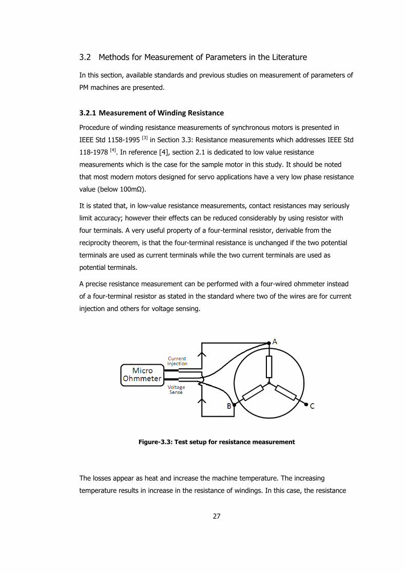
27

3.2 Methods for Measurement of Parameters in the Literature

In this section, available standards and previous studies on measurement of parameters of

PM machines are presented.

3.2.1 Measurement of Winding Resistance

Procedure of winding resistance measurements of synchronous motors is presented in

IEEE Std 1158-1995 [3] in Section 3.3: Resistance measurements which addresses IEEE Std

118-1978 [4]. In reference [4], section 2.1 is dedicated to low value resistance

measurements which is the case for the sample motor in this study. It should be noted

that most modern motors designed for servo applications have a very low phase resistance

value (below 100mΩ).

It is stated that, in low-value resistance measurements, contact resistances may seriously

limit accuracy; however their effects can be reduced considerably by using resistor with

four terminals. A very useful property of a four-terminal resistor, derivable from the

reciprocity theorem, is that the four-terminal resistance is unchanged if the two potential

terminals are used as current terminals while the two current terminals are used as

potential terminals.

A precise resistance measurement can be performed with a four-wired ohmmeter instead

of a four-terminal resistor as stated in the standard where two of the wires are for current

injection and others for voltage sensing.

Figure-3.3: Test setup for resistance measurement

The losses appear as heat and increase the machine temperature. The increasing

temperature results in increase in the resistance of windings. In this case, the resistance

28

value measured at room temperature will not be accurate for analytical calculations. For

any winding temperature, resistance of the windings at room temperature can be

corrected with equation (3-1).

ph

o

ph RT

TR ×

+

+=′

5.234

5.234 (3-1)

This modified resistance R’ph value may be used instead of resistance at room temperature

Rph in analytical performance calculations to get more accurate results in operating

conditions.

3.2.2 Measurement of Inductance

Inductance measurement is a special problem for all electrical machines but in PM

machines it is an attractive field of theoretical and practical studies. Studies on parameter

measurements in the last three decades have investigated measurement of inductance of

PM machines and still efforts go to this area.

Although motor performance measurement methods in standards can be easily adapted to

PM machines, parameter measurement tests for synchronous and induction machines

dealing with reactances (equivalently inductances) are difficult to interpret or even

inapplicable to PM machines due to presence of magnets as a constant flux source. That is

why standard procedures to measure inductance cannot be applied to PM machines.

Accurate inductance measurement results are important for modern high performance

motor drives. Since conventional machines are replaced by PM machines, more work is

done to improve the overall electromechanical performance of “drive + motor” systems.

Dynamic and steady-state performance analysis and precise control of PM machines

depend on accurate equivalent circuit models of the system with correct parameter values.

i. Measurement of Quadrature-axis synchronous reactance Xq in Standards

Quadrature axis synchronous reactance Xq is defined in [5] as the ratio of the fundamental

component of reactive armature voltage due to the fundamental quadrature-axis

component of armature current, to this component of current under steady-state

conditions and at rated frequency.

This definition can be clarified on a phase diagram. In Figure 3.4, reactive armature

voltage due to quadrature-axis component of armature current is the vector of “Iq.Xq” seen

on top of the figure. So if amplitudes of “Iq.Xq” vector and q-axis armature current “Iq” are

extracted, Xq can be determined.

29

Figure 3.4: Phase diagram for a synchronous machine [3]

The standard [3] proposes four different methods under Section 10.4 to determine Xq.

Two of these tests (Sections 10.4.2 and 10.4.3 in [3]) require zero field excitation, so they

are not applicable to PM machines. One other method (Section 10.4.4 in [3]) proposes an

empirical function of motor dimensions to calculate Xq/Xd ratio and determining Xq from Xd

value which is far from being accurate and reliable.

The last method (Section 10.4.5 in [3]) states that load angle determination may be used

with voltage and current measurement to determine Xq. This is most applicable where

determination of internal load angle is necessary. The definition of internal load angle “δ”

is given in IEEE Std 100-1992 as follows: “The angular displacement, at a specified load,

of the center-line of a field pole from the axes of the armature MMF pattern.”

In section 10.8.2 in [3], various load angle determinations are presented:

i. calculation of internal load angle

ii. stroboscope technique of measurement,

iii. electronic measurement of load/phase angle

Among these, the last method of electronic measurement is more applicable in the sense

of available laboratory equipment. In this method, internal load angle is measured by

comparing the phase difference between a once-per-pole-pair pulse on the shaft and a

“squared-off’ terminal voltage signal.

ii. Measurement of Direct-axis synchronous reactance Xd in Standards

Direct axis synchronous reactance Xd is defined in [5] as “the quotient of a sustained value

of that fundamental alternating current component of armature voltage that is produced

by the total direct-axis flux due to direct-axis armature current and the value of the

30

fundamental alternating-current component of this current, the machine running at rated

speed”.

The standard [3] proposes one method in Section 10.3 to determine Xd which states that

the synchronous impedance Xd in per unit is equal to the ratio of the field current at base

armature current, from the short-circuit test, to the field current at base voltage on the

air-gap line. Since there is no field excitation in PM machines this method can not be

applied.

iii. Measurement of Xd and Xq in the Literature

In this chapter, previous studies in the literature on PM machines inductance measurement

presented are investigated. It is evident that it is impossible to cover all the studies, but a

selection may be done among them to summarize the proposed methodologies about the

topic.

Methods mentioned in the literature generally depend on the PM machine phase diagram

presented in Figure 3.5. The figure is similar to Figure 2.4 in CHAPTER 2. The angle

between motor phase voltage Vt and back EMF Eo is motor load angle “δ”. When talking

about d-q axes parameters (Eo, Ld, Lq, Xd, Xq, Id, Iq), this phase diagram should be

considered.

Figure 3.5: Phase diagram of PMSM at normal operation

Note: Vectors in the figure are exaggerated for clarity.

31

Having investigated many of the studies, a number of common features of the proposed

methods are determined which can be listed as follows:

i. What is the aim of the study? ii. What kind of machine is tested? iii. What method is used to drive the tested machine? iv. What is the measurement method? v. Is load angle measured? How? vi. Is frequency dependence of inductance investigated? vii. Is current (or equivalently load) dependence of inductance investigated? viii. Is cross-coupling between d-q axes components investigated? ix. Does Eo vary with current (or equivalently load)? x. What is the comment of authors about the results? xi. Is the offered method suitable to apply on the test motor in this thesis work?

Selected papers from respected authors will be analyzed in terms of the determined

features and presented in following sections in chronological order. Results and

interpretations will be discussed in each section. At the end, inferences will be tabulated to

have an overall view.

Study.1

Author: TJE Miller [13], 1981

The study by Miller is one of the first attempts to measure d-q reactances of a 1.5 kW

internal magnet PM machine. Two different measurements are proposed; load test at

running conditions and static (standstill) inductance measurement.

In standstill tests, the degree of interaction between d-q axes quantities is tried to be

measured with a special double bridge circuit which is illustrated in Figure 3.6. Motor

windings are connected in d-connection (phase B-C terminals are short circuited) and

excited with dc while rotor is fixed at 0° (rotor is aligned with phase A magnetic axis). In

the circuit, secondary voltage source V2 biases the windings with q-axis current without

disturbing the balance of main bridge circuit. This second dc bias does not contribute to d-

axis flux because d-axis MMFs of phase B and C cancel each other. Static flux linkage

measurements were done to determine reactance variations while controlling d-q axes

currents independently.

32

Figure 3.6: Double bridge circuit for measuring the interaction between d-q axis

parameters [13]

In the load tests, the tested motor is driven directly from the line with an adjustable load

coupled to the shaft. Line current is varied by adjusting the load. Voltage, current, power

factor and torque angle are recorded to define the phase diagram. Load test

measurements are conducted only in 50Hz by driving tested motor directly from line, so

frequency dependence is not investigated. Back EMF voltage Eo is assumed to be constant

at the value determined at rated motor speed. Variation of reactances Xq and Xd are

investigated with respect to line current (Figure 3.7). The method of determining the load

angle is not specifically defined but two methods have been proposed; stroboscopic

illumination of a graduated disc attached to shaft, or clamping a collar to the shaft with a

magnetic projection which produces a pulse to trigger line voltage waveform on

oscilloscope. Results of this study are presented in Figure 3.7 and Figure 3.8.

33

Figure 3.7: Results of Xd and Xq measurement from load tests by Miller [13]

Figure 3.8: Ld variation with Id and its interaction with Iq from standstill test [13]

From presented curves by Miller, it can be concluded that;

Xd is not measurable at a specific line current where Id equals zero. This is an

expected result since the measured current and load angle quantities become very

small and calculations are susceptible to measurement errors. Beyond this point,

Xd dramatically rises with negative Id whereas Xd doubles with positive Id at rated

line current (Figure 3.7).

Xq measurements are available for 0.5 - 1.0 p.u. line current. In this range, Xq

decreases to 25% of initial value (Figure 3.7).

Ld increases by 50% up to 0.8 p.u. magnetizing Id while Iq=0. Increase in Ld is

suppressed in Iq=1 p.u. case where Ld value is same for Id=0 and Id=1 p.u.

34

(Figure 3.8). The increase of Ld with Id is unexpected result. Common sense is a

constant inductance value or decrease with current due to saturation.

Ld increases by 10% with demagnetizing Id while Iq=0. In presence of Iq=1 p.u.,

Ld decreases by 25% with 0.5 p.u. demagnetizing Id then this value restores to

initial Ld value with Id=1 p.u. (Figure 3.8).

Ld - Xd variations of standstill and load tests do not agree with each other in

demagnetizing condition. The dramatic increase in Xd in load tests is not observed

in standstill tests where Ld is constant for a wide range of Id current. This is

probably due to cross coupling between d-q axes components and constant Eo

assumption in load tests. Xd is plotted against line current for load tests which may

not be comparable with Ld - Id variation where only Id is present

Miller concludes that “saturation characteristics of PM motors make it impossible to

specify Eo and Xd uniquely because there exists only one equation for two

unknowns; Any value quoted for Xd must be associated with a specified (arbitrary)

value of Eo, such as the true open circuit”. This statement refers to a need for

constant Eo assumption because as seen in Figure 3.19-a, it is not possible to

separate Eo and Xd with one d-axis voltage equation. One of them must be

assigned with a value. Also it is stated that bridge method does not produce

results of highest precision, but may be used to enhance the level of confidence in

Xd and Xq values determined from load tests.

The other conclusions from this study can be summarized as follows:

The load tests offered by Miller depend on extraction of load angle.

Neglecting resistance of the windings as in the study is not acceptable in case of

voltage drop on resistance is comparable to back EMF voltage Eo and must be

inserted in the phase diagram.

The inductance bridge method is not practical since stability of resistances in the

circuit may not be controlled due to thermal changes with high currents (17Arms

rated for this thesis work).

Hysteresis effects may produce scatter in calculated reactance results which is also

mentioned by the author of this study.

35

Study.2

Author: B.J. Chalmers [14], 1985

Chalmers et al [14] tried to determine reactances of the tested 275W, 100V, internal

magnet PM machine based on two-axis machine theory. In the study, identification

method of parameter estimation offered by Eykhoff [11] is applied and a new method which

searches for Id=0 condition to measure specifically Xq is proposed. The tested motor is

driven with scalar control at different frequencies between 7.5Hz and 50Hz for the full

360° range of load angles at various supply frequencies. Voltage, current and power is

measured at motor terminals for each operating condition. The load angle was measured

using a stroboscope that is triggered by the sinusoidal motor phase voltage. Applied

methods require measuring input current and power at a particular supply voltage, for a

range of load angles in the range 0-90°. From these measurements, with the knowledge

of load angle, Id and Iq are evaluated with respect to Figure 3.5. Curves of Id and Iq

against load angle are then constructed and the point where Id = 0 is found. Xq is

calculated at that point. In this study, Xq – Iq relation is identified (Figure 3.9). Results of

frequency dependence of reactances are not illustrated as a figure, but explained in words

instead.

Figure 3.9: Results of the study by Chalmers et al. [14]

36

Chalmers et al concludes that;

Excitation EMF Eo and d-axis reactance Xd are substantially constant under varying

load, which is due to high coercive magnets on d-axis.

Phase resistance R varies from its cold value, in regions of small load angle (0< δ

<90°), to about double that value at high currents (120°< δ <300°, see Figure

3.9-a). This variation is mainly attributed to temperature rise during the tests. This

result

A cyclic variation of Xq0 with load angle is observed. This variation was clarified

when Xq0 was plotted against Iq (Figure 3.9-b), showing that Xq0 followed the

same curve for both positive and negative values of Iq.

The only statement about frequency dependence is as follows; at rated torque, Id

is negative and its magnitude decreases as frequency is decreased. At the same

torque, Iq increases as frequency is decreased. This causes Lq0 to decrease owing

to saturation, as in Figure 3.9-b. This relation, which says that Lq decreases with

decreasing frequency, is not illustrated but interpreted depending on Id - Torque

and Iq - Torque curves.

Besides these conclusions, it is evident that the offered method to measure Xq by seeking

Id=0 condition through measurements is useful but primitive in presence of a vector

control drive since Id=0 condition, which is sought through measurements, can be easily

satisfied. However the interpretations of the author on the results are important.

Study.3

Author: S.F. Gorman et.al. [42], 1988

In this work, authors try to determine synchronous reactance of an internal PM motor

(0.55kW, 380V, 1.10A). The tested motor is driven as a generator by an auxiliary DC

motor. A balanced three-phase load is placed across the terminals of the tested machine.

The load angle is determined with a stroboscopic pointer system. Xd and Xq are

determined by solving d-q axis voltage equations for each particular set of data (phase

voltage and current, power factor angle, load angle, back EMF voltage). Back EMF voltage

Eo is assumed to be constant at the value that is measured at motor terminals at no load

at rated speed. DC value of phase resistance is inserted into d-q axes equations. The test

is conducted for a single current value (for a single load condition) which does not give

37

variation of parameters with current and cross relation between d-q axes. Also frequency

dependence is not studied.

Although this is not a comprehensive study, operating the PM machine as a generator is a

different approach regarding other presented studies. If a variable three phase balanced

load is available, which is fully characterized before the test in terms of resistance and

inductance, one can determine the internal reactance of the motor by loading the motor at

constant speed. At first step, the motor is driven by auxiliary machine and emf at motor

terminals is observed. The observation must be done by triggering the measurement by

means of a pulse generator attached to the rotor shaft which outputs a pulse per

revolution. The observed waveform at motor terminals at this condition is internal emf

voltage of the tested motor which is also zero load angle. Depending on loading, the

observed voltage waveform will shift in terms of amplitude and angle because the current

in the windings will result a voltage drop on internal resistance and inductance. For each

specific loading case, defined set of data (phase voltage and current, power factor angle,

load angle, back EMF voltage) must be recorded. By resolving the current into d-q

components, Xd and Xq can be determined for that case from the phase diagram related to

the operating condition.

There may be cross coupling between d-q axes components since Id and Iq are present at

the same time. However, at low current, cross coupling between axes may be assumed to

be negligible and unsaturated d-q axes can be determined.

The weakness of this method is that d-q axis currents can not be controlled independently.

For example, a pure q-axis current can not be drawn from the machine because it will not

be in-phase with back EMF voltage Eo due to introduced phase by reactance of the

windings and load. The same situation is valid for d-axis case.

Study.4

Author: P.H. Mellor et al. [16], 1991

Mellor et al [16] pointed out the difficulty of load angle measurement and tried to avoid

dealing with load angle by an iterative solution of the two axis theory. A static inductance

bridge test, no-load and load tests are conducted to determine Xd, Xq and Eo and their

variation with current (or equivalently load). The tested motor (4-pole, internal magnet,

8Arms rated, D60 frame motor with damper bars in the rotor) is driven by terminal voltage

control. The equations to determine parameters from measurement data are based on the

PMSM phase diagram (Figure 3.5) and two-axis motor model (Figure 2.3).

38

By running the machine at no load, the permanent-magnet excitation Eo at zero armature

reaction and the core loss resistance Rc are identified.

sat RIVE −=0 (3-2)

a

cI

ER 0= (3-3)

The direct-axis synchronous reactance Xd is measured by performing the no-load test over

a range of terminal voltages to vary the terminal current. At each load current, Xd is

calculated from internal voltage Ei and current Id using equations (3-4), (3-5) and (3-6). In

the equations Vt is phase voltage, Ia is phase current, φcos is power factor.

d

i

dI

EEX

0−= (3-4)

φcossati RIVE −= (3-5)

21

2

22

−=

c

iad

R

EII (3-6)

Figure 3.10: Equivalent circuit diagram of PM machine at no load

To determine Xq from a load test, a rotor sensor is used to index the direct axis alignment

of one winding and adjusting the motor load and voltage until the terminal current is in-

phase with back EMF Eo (Id=0 condition). This is also the vector control condition. The

phase diagram for this particular case is shown in Figure 3.11 and Xq is calculated by

equation (3-7).

39

Figure 3.11: Phase diagram when Ia is on q-axis

(Ic neglected)

a

t

qI

VX

φsin= (3-7)

Frequency dependence of parameters is not investigated since running tests are

conducted at single speed (only 50Hz).

Besides running tests, an inductance bridge method is conducted at standstill to determine

reactance variation which is similar to Miller’s method. To obtain correct level of

saturation, a DC current corresponding to peak value of current at running condition is

supplied to the bridge. Measurement results of this work at 50Hz are presented in Figure

3.12.

40

Figure 3.12: Variation of Xq, Xd and Eo by Mellor et al [16]

In Figure 3.12-a, it is shown that there is a cross coupling between Id and Xq where a

rated current in direct axis will cause approximately a 10% change in Xq. About 100%

increase of Xd in negative Id region in Figure 3.12-b is explained by a fall of the excitation

field as a result of increase in the leakage around the magnet during demagnetization. On

the other hand, a rated magnetizing current decreases Xd by 10%. Eo decreases by 15%

with increasing Iq which is explained by higher level of saturation in the rotor poles with

increasing Iq. Another fact is that results of standstill and running tests agree with each

other.

The offered no load and load tests are easily applicable in presence of vector controlled

drive since d-q axes current can be controlled independently. The inductance bridge

method by the author may not be practical to apply since it is hard to maintain the stability

of the bridge circuit under excessive currents if the motor has high current ratings.

41

Study.5

Author: M.A. Rahman, Ping Zhou [39], 1994

Rahman and Zhou [39] tried to determine saturated Xd, Xq and Eo parameters of a PM

motor and variation of Eo with load. The tests are conducted on a 1 hp, 4 pole, interior PM

motor which is driven from a 60Hz line with voltage control method. A variable load

coupled to the shaft is used to alter load angle.

Load angle was detected by with a micro-processor based digital setup. As the authors

stated; for motoring operation, when the zero crossing of any one of the three phase

terminal voltages as the reference to initiate a pulse and the zero crossing of the magnet

excitation voltage in the same phase winding to terminate the pulse are used, the resulting

pulse width will then represent the instantaneous torque angle. For generating mode, the

reverse will happen.

This study is based on the fact that d-q phase diagram of PM machine includes both three

unknown parameters Eo, Xq and Xd but only two voltage equations (equations (2-5) and

(2-6)) can be formed. This problem is solved by obtaining a third equation with a slight

change of the load where it is assumed that back EMF and inductance does not change

under this condition or the change can be ignored.. It is not defined how much the load is

changed however Stumberger et al [17], who repeated Rahman’s work with a different

setup, defined this change as varying the load so that 0.1o change in phase angle between

terminal voltage and current occurs. The derived third equation together with the other

two equations related to d-q axes are as follows.

qii XIE δδ sinsin = (3-8)

doii XIEE βδ coscos += (3-9)

doii XIEE βδ ′′+=′′ coscos (3-10)

In the equations, Ei is motor phase voltage, I is phase current, δ is load angle, and β is

motor current phase angle with respect to stator magnetic field d-axis. Xd and Eo are

separately determined with equations (3-16) and (3-25). The result of the offered method

is presented in Figure 3.13.

42

Figure 3.13: Variation of Xd, Xq and Eo by Rahman et al. [39]

The results of Stumberger’s [17] similar work to Rahman’s is presented in Figure 3.14.

Stumberger conducted the tests on a 0.67kW, 380V, 1.49A 4-pole internal PM machine. In

the figure, variation of Xd and Xq is investigated against motor load angle which is

equivalent to investigating by motor terminal current and also variation of induced voltage

due to magnets in dependency on internal load angle at line to line voltages 210V. 230V

and 270V are presented.

43

Figure 3.14: Variation of Eo, Xd and Xq at different terminal voltages

by Stumberger et al [38]

Results of both Rahman’s and Stumberger’s work show that Xd does not vary much with

load. On the other hand Xq considerable decreases (40% decrease in Rahman’s work, 25%

decrease in Stumberger’s work) with increasing load. The increase in Eo in Rahman’s

solutions is not expected to be the real case, because Eo should be decreasing due to

saturation of steel core with high load. It is probably due to flux enhancing with Id current

injection since vector control is not applied during the defined tests.

The offered method to alter the load angle by 0.1o is very problematic because a very

precise test setup and measurement is needed which may be unrealizable in most

laboratory environment. Also this very little change may not be determined even

completely digital setup is used to detect load angle (instead of analog measurements like

stroboscope) due to measurement errors. In conclude, this method does not seem to be

practical to apply.

44

Study.6

Author: Fidel et al. [18], 2001

In this study variation of inductances with currents are investigated based on two-axis

model. The tested motor is 220V 7A 2000rpm PM machine and it is driven by vector

controlled inverter drive. The current, voltage and power are feedback to inverter through

a current controller. The measured quantities are transformed to d-q rotating frame to do

calculations. The tested motor is loaded with an induction motor which is controlled with

an inverter. The tested motor is driven successively under Id=0 and Iq=0 conditions. At

each case the other non-zero axis current is varied up to rated value. Then Ld and Lq are

calculated with equations (3-11) and (3-12) respectively which are extracted from

equivalent electric circuit model (Figure 2.3).

(3-11)

(3-12)

Inductance results of this study is presented in Figure 3.15.

Figure 3.15: Experimental values of Ld and Lq respectively by Fidel [18]

(Dashed lines show measurement uncertainty)

45

Frequency dependence of inductances is studied by repeating the experiment at rated

frequency (60Hz) and one-third (20Hz), but no significant difference due to frequency is

reported. On the other hand, a 15% increase in Ld with Id and 10% decrease in Lq with Iq

are observed respectively (Figure 3.15). At very low currents, the authors recommend

using an electronic bridge at standstill to determine d-q inductances and result is

presented in Figure 3.15 using symbol “o” on the left axis.

Any comment on the results ox Ld and Lq variation is not presented by the authors. As

seen in Figure 3.15, Lq decreases with increasing Iq which is probably due to increase in

saturation level of q-axis flux path. Ld has an increasing trend with negative Id which can

also be related to saturation level of associated d-axis flux path. Also in the results,

uncertainty in the estimation of parameters rapidly increases as current decreases with the

offered method.

Variation of Eo is not studied in this study. However determination of core loss (or

equivalently iron loss) resistance Rc is stated to be very important. Rc is measured at no

load with low current to reduce copper losses which can be achieved by setting Id=0 and

Iq sufficiently big to compensate mechanical losses at the operating speed. At this

condition, current component Ioq in Figure 2.3 is zero and Rc can be calculated by;

in

q

cP

VR

2

= (3-13)

where Vq is motor terminal voltage and Pin is measured input power. The phase resistance

Rs is ignored in equation (3-13) since Rc has about 50-100 times higher value than Rs.

The offered test method by the authors is applicable to our machine since the same test

setup is available and vector control drive is also present. The procedure is also straight

forward and easy to follow.

Study.7

Author: R. Dutta, M.F. Rahman [44], 2006

In this work, authors compare the results of FE analysis, AC standstill and vector current

control tests by applying them to a prototype IPM machine (rated as 550W, 14A, 20.2V) at

same current levels. The obtained values from the tests are compared and differences are

analyzed. The inductances were also computed from the finite-element (FE) model of the

same machine to verify the findings.

46

FFT algorithm is applied to the measured voltages and currents to extract the fundamental

components and then the rotor frame d-q transformation is applied to obtain d-q axis

voltages and currents since d-q axes voltage equations (2-14) and (2-15) related to

equivalent phase diagram of the motor PM motor is valid only for fundamental harmonic.

In running tests, load angle is not measured because Id and Iq currents are controlled by

vector control and load angle is determined with respect to power factor and motor

terminals (see Figure 3.19).

Frequency dependence is not studied by the authors. The influence of cross coupling

currents over the flux linkages is investigated through standstill tests. Phase resistance Rs

is taken into account in both tests. The obtained inductance measurements with respect to

current together with FE results are presented in Figure 3.16.

Figure 3.16: Variation of d-q inductances with current obtained from standstill and

vector control tests by Dutta et al. [44]

In Figure 3.16, variation of Lq and Ld with current obtained from two test methods and FE

calculations are compared respectively. AC standstill and flux linkage FE results agree for

Lq, but vector control test gives out 33% larger Lq value (Figure 3.16-a). This result is

explained by authors as cross coupling saturation of q-axis flux path by d-axis flux which

includes both magnet flux and flux due to Iq current since they share the same flux path.

The ac standstill test and three-phase flux linkage FE method also give almost constant Ld

values throughout the whole current range, whereas in the other two methods, Ld rises

steeply when current is low (Figure 3.16-b). Authors explain this result with the saturation

level of iron bridges in the rotor structure. In some motor structures, influence of current

47

over d-axis flux is minimal if iron bridges are fully saturated by the leakage flux between

two adjacent magnet poles. However, in some of the rotor structures, the iron bridges

may not be fully saturated by the magnet leakage flux alone and neither small Id current

can saturate them. In this type of situation, d-axis flux linkage is relatively higher, which

results in a larger Ld for low current.

The effect of q-axis current on d-axis magnet flux linkage (cross coupling) is also studied.

The effect of 10% error in magnet flux linkage on the calculated Ld is shown in Figure

3.17. It can be concluded from the result that constant back EMF voltage assumption

under varying load is not truly correct and the change in magnet flux linkage due to the

temperature rise should be included.

Figure 3.17: Variation of magnet flux linkage with Iq and change of Ld with different

magnet flux linkage assumptions by Dutta et al. [44]

This study is an example of good approach to inductance measurement where different

methods are applied and results are compared. The offered AC standstill, FE and load tests

are easy to conduct.

Conclusion to Literature Review

Up to now, details of selected studies are summarized. Each of them is analyzed in terms

of the features that are defined at the beginning of this section. To have an overall view of

studies and to compare with each other easily, methods and results of these studies are

tabulated in Table 3.4.

It can be observed in presented methods in the literature that most effort is on

measurement of inductance of PM motors because it is most problematic topic. Other

48

motor characterization tests such as resistance measurement or torque-speed

determination has straight forward procedures which are standardized for many motor

types. However, very recent studies can be found on inductance measurement of PM

machines which shows that methods for measurement of inductance are not mature yet to

be standardized.

The presented various methods can be classified with respect to methodologies as in

Figure 3.18. In the figure, proposed tests are grouped into two at first stage; Standstill

Tests (where motor is not operated and the shaft is not rotating) and Running Tests

(measurements are made online while the motor is rotating). Each group is divided into

subgroups where load angle measurement is distinctive for running tests and excitation

scheme is decisive for standstill tests.

The proposed load and no-load tests are realized either by connecting the tested motor

directly to AC line or with a vector controlled drive. Since all presented methods can be

realized with a vector control drive, this approach seems to be the most proper method to

conduct running tests. In the running tests, half of the studies determine load angle of the

tested motor at each operating condition, whereas the others accept that since axis

currents can be independently controlled, power factor (PF) angle Ø can be used directly

to determine the load angle. It is evident that load angle measurement is a must without a

field oriented drive because there is no other way to decompose measurement quantities

into d-q components. However, if there is a vector control, where d-q axes components

are independently controlled, load angle can be determined from PF angle. For example, if

Id=0 condition is valid then load angle δ equals to PF angle Ø (Figure 3.19-a), and if Iq=0

condition is valid then load angle δ equals to “90- Ø” (Figure 3.19-b).

49

Table 3.4: Comparison of inductance measurement methods

50

Table 3.4 contd. - Comparison of inductance measurement methods

51

From Table 3.4, following observations can be made:

• Majority of the studies are performed on an internal magnet PM motor where

magnets are placed inside the rotor steel. This shows that there is lack of

attention about inset (for surface also) magnet PM machines.

• Proposed tests can be grouped in two; Standstill Tests (where motor is not operated

and the shaft is not rotating) and Running Tests.

• Load angle measurement is distinctive for running tests and excitation scheme is

decisive for standstill tests.

• Early works used stroboscope to determine load angle. Recent works used an

encoder coupled to motor shaft for load angle extraction. Also vector control

scheme is used in some recent works where load angle equals to power factor

angle at motor terminals.

• Authors who use Load Test method (Miller, Chalmers, Mellor, Rahman, Stumberger,

and Fidel) agree that either Xq decreases with Iq. Only Dutta states that no

significant variation of Xq occurs with Iq.

• For Xd measurement; Miller, Mellor states that Xd decreases with positive Id and

increases with negative Id. Fidel agrees with these authors for negative Id case. On

the other hand Chalmers, Rahman and Stumberger states Xd remains constant

with Id. Dutta reports two different results where Xd remains constant in AC

standstill test and decreases steeply with Id in Load Test.

• Back EMF Eo may decrease with Iq (or equivalently) depending on the saturation of

flux paths which is totally dependent on motor structure. Miller, Chalmers, Mellor

and Fidel assume Eo to be constant in no-load tests. However Mellor and Dutta

reports Eo decreases with Iq as observed in load tests.

• Frequency dependence of the inductance is studied by Chalmers, Mellor and Fidel.

Only Chalmers report that Lq decreases with frequency. Others state that

inductances do not vary much with frequency.

• Miller, Mellor and Dutta studied cross coupling between axes. Common statement is

that inductances may decrease by cross axis current due to increased saturation.

• The proposed load and no-load tests are realized either by connecting the tested

motor directly to AC line or with a vector controlled drive. Since all presented

methods can be realized with a vector control drive, it seems to be the most

proper method to conduct running tests.

52

• All authors except Dutta agree that Xq (or equivalently Lq) decreases with line

current. Dutta states that the variation is insignificant. This is probable since the

decrease in Xq may arise in case of saturation in q-axis flux path. If there is no

saturation then a constant value may be determined from the test.

• For Xd measurements, all authors except Fidel reports that Xd (or equivalently Ld)

stays constant or decreases in some extent with line current. Fidel states an

increase in Xd value with negative Id (about 12% difference between full load and

no load) which is probably due to demagnetizing effect of negative Id on

saturation level of the d-axis flux path.

Figure 3.18: Proposed inductance measurement methods

53

Figure 3.19: Phase diagrams related to Id=0 and Iq=0 cases

• The studies depending on load angle measurement requires detecting the load

angle of the tested motor both at no-load and under load to determine load angle

deviation. There is a need for a stroboscope system which may be triggered with

an external pulse generator per rotor revolution or a position encoder.

• The inductance bridge method seems to give satisfactory results however it is very

difficult to construct a stable bridge circuit at high current levels. In this thesis

work, the rated current of the tested motor is 17 Arms which may result dissipation

of considerable amount of energy on circuit elements. On the other hand,

standstill AC excitation is simple to conduct in a laboratory environment, but

monitoring of the winding temperature during the measurements and correction of

the winding 20°C (cold) resistance values for operating temperatures is a very

important issue [40].

• DC decay tests are simple but interpretation of the results is important. It is

evident that an exponential decay waveform has at least two time constants; sub-

transient and transient. Although standstill tests give out some inductance values,

they do not simulate the real phenomena in the motor under normal operating

conditions. DC decay test results can be relied on solely. In fact they should be

conducted in conjunction with running tests to compare measurement results.

In conclude, since different methods give different results even on the same PM machine,

any parameter measurement should be performed under the same conditions of normal

54

operating. If vector control is used to drive the motor in normal conditions, then

parameter measurement should be also performed with vector control to be able to define

two-axis model of the tested PM machine. However, it is wise to conduct all the proposed

tests (standstill DC decay, standstill AC, no load and load tests, FE analysis) on a tested

PM machine to completely characterize the inductance variation of a PM machine. The

results of all measurements should interpreted together to determine inductance variation

phenomena for the tested motor. While conducting tests, current and frequency

dependency of measured quantities should be analyzed to have a full understanding.

3.2.3 Measurement of Back EMF Voltage

The back EMF is the voltage generated at stator windings due to time variation of linkage

between rotating magnet flux and stationary stator windings.

There are no methods in [3] to be applied for emf voltage measurement. However the

method for “Open-circuit saturation curve” defined in Section 4.2.5 in [3] can be modified.

This method states that open circuit saturation curve is obtained by driving the tested

machine at rated speed, open-circuited, and recording its armature terminal voltage.

Since field can not be adjusted in PM machines, speed can be varied instead of field

current. This will give armature terminal voltage variation with respect to speed which is

emf voltage variation with speed also. It is shown in Chapter.2 that amplitude of the

terminal voltage is linearly dependent to rotational speed of the rotor as seen in equation

(3-14). Since field excitation is constant and ke is a function of flux linkage, the linear

relation between open circuit terminal voltage and shaft speed is expected.

mecheo wkE ×= (3-14)

3.2.4 Measurement of No-Load Loss

There is no sense to imagine a system that converts energy from one form to another with

100% efficiency. Inevitably there is always an amount of lost energy that is not utilized. In

PMSM (whether generating or motoring) some electromechanical work is lost and radiated

as heat. Those losses can be listed as;

1. Copper losses

2. Friction and Windage losses

3. Core losses

55

Copper losses are modelled with a resistance in electrical model of the PMSM. Friction and

windage losses are measured and taken into consideration as a reduction in output torque

of the motor. Beside these losses, core losses arise in lamination (core) due to time

variation of flux.

Procedure of friction-windage and core loss measurements of a synchronous motor is

defined in “Section 4.2.7: Core loss and friction and windage loss” of reference [3].

In this case, the machine under test is usually driven by a motor, directly or through a belt

or gear. It is stated that the friction and windage loss is obtained as the power input to the

machine being tested, through auxiliary drive, with zero excitation. The tested machine

should be fully demagnetized. The core loss at each value of armature voltage is

determined by subtracting the friction and windage loss from the total power input to the

machine being tested while the tested machine is excited with rated field current.

For PM machines, zero excitation is not realizable since magnets act as a permanent

excitation source. In this case, friction-windage and core loss can not be separated from

each other. The two torque components cannot be separated unless magnets are removed

from the rotor. This is not feasible for most motors and disassembling a motor may result

in performance drop.

The mechanical power input to the tested PM machine (with open terminals) driven by an

auxiliary motor has to be measured by some means (most applicably with a torque

transducer) and the measurement value has to be accepted as total of friction-windage

and core loss.

3.2.5 Measurement of Motor Thermal Constant

In this test, motor is loaded with specific load at a constant speed. The test is carried on

until the motor reaches a thermal equilibrium with the ambient. The test speed and load is

totally subjective, but it must be noted that the load must not be too high to avoid

reaching a thermal equilibrium.

During the test, motor temperature must be sampled. In this work, a thermistor placed in

stator end-winding of the test motor is used to monitor temperature variation in every 5

minute. It is assumed that, all points of the test motor reaches nearly same temperature

value in the thermal balance. This is acceptable as there is no forced cooling for this

motor.

When the thermal balance is reached, temperature difference between the motor and

ambient is accepted as the temperature rise due to losses in the motor. Motor losses are

56

calculated by subtracting output power from total input power to motor. By dividing power

loss of the motor to temperature rise, thermal constant of the motor can be derived.

3.2.6 Measurement of Torque-Speed Characteristic

Methods for determining speed-torque curves of a synchronous motor are defined under

Section 7.3 in reference [3]. Among proposed methods, “Method.4: Direct Measurement”

method defined in section 7.3.5 is most applicable. This methods states that output torque

can be measured by loading the tested machine at various speeds with a dynamometer or

prony brake. This requires the maintenance of constant speed for each reading. Sufficient

test points should be recorded to ensure that reliable curves, including irregularities, can

be drawn in the regions of interest from the test data. Two different torque-speed

characteristic may be determined which include rated and maximum current conditions.

3.2.7 Measurement of Efficiency

Efficiency measurement procedure is defined in “Section 4.6.2, Method 2: Input-output” of

reference [3]. The efficiency from the input-output method is determined as ratio of

output power to input power. The electric inputs (voltage, current, phase angle) to motor

are measured with instruments. The output of the motor is measured with a dynamometer

preferably.

3.2.8 Measurement of Cogging Torque

Cogging torque results from attraction of rotor magnets with stator teeth. Rotor tends to

align itself with minimum reluctance. If the rotor is rotated, this alignment torque can be

detected at rotor shaft as a ripple. In low speed and sensitive applications (i.e. drive-by-

wire systems where automobile steering is done with an electric motor), minimum cogging

torque is desirable.

It is proposed by Boldea [40] that an auxiliary motor with a very low torque ripple can be

used to turn slowly (2-4 rpm) the rotor of the motor under test. An additional inertia may

be placed on the shaft to increase the accuracy of the measurement. The accuracy of

cogging torque measurement depends on preservation of shaft speed at a fixed speed.

Fluctuation of the speed during cogging measurement will result in sideband torques

around expected frequencies.

57

3.2.9 Conclusion to Measurement Methods Section

In the following chapters selected methods will be applied to the sample motor that this

thesis work deals with. The aim of this section is to determine the variation of inductance

with different test methods so that a comparison of offered methods may be done with

respect to accuracy and dependency.

3.3 Applied Test Methods and Approach and Measurement Results

In the previous section, available standards and test methods for measurement of PM

machine parameters are determined. In this section, the selected methods are to be

applied to the tested motor and the results are presented.

The tested motor which is specified in Section 3.1 is a PM motor with inset mounted

magnets. There is a saliency between adjacent magnets on the rotor to enhance the rotor

mechanical structure which makes quadrature and direct axis parameters differ from each

other. It can be observed in the presented studies in Section 3.2, there is no much effort

on surface and inset magnet motors.

There is a vector controlled driver available for this thesis work which enables independent

control of d-q axis excitation of the motor. There are parameter measurement studies with

vector control drive ([18], [44]) however the tested motors are internal magnet motors.

From this point of view, this thesis work explores application of offered methods to inset

magnet motors (also applicable to surface magnets).

An overview of the tests to be conducted for PMSM parameter determination can be

summarized as in Figure 3.20.

Figure 3.20: Overview of the Measurement Procedures for PMSM

PM Motor Tests

Standstill Tests Running Tests

Resistance

Inductance

Torque

No-Load Tests Loaded Tests

EMF

Iron Loss

Friction & Windage

Torque-Speed

Efficiency-Speed

58

3.3.1 Result of Resistance Measurement

In this work, four wired measurement method defined in Section 3.2.1 is applied where

“Agilent 34420A Micro Ohm Meter” device is used and 0.140Ω is measured at terminals of

the PM motor (line-line) at 20°C room temperature. To get per phase resistance, the

measured value is divided by two, resulting 0.070Ω.

3.3.2 Results of Inductance Tests at Standstill

These studies focus on standstill tests to measure inductance because it is problematic to

extract load angle when the motor is operating. Many modern motor drives have pulse

width modulated (PWM) voltage output. Measuring the fundamental harmonic of terminal

voltage of the motor may require special treatment. Beside exciting the motor terminals by

PWM waveform, excitation with AC-source with variable voltage and frequency [13], [31],

[36] or using a DC current decay setup [31], [37] may be used also to extract

inductances. Frequency dependence and current dependence of inductance is studied to

fully characterize inductance variation for different motor operation conditions.

i. Results of Inductance Measurement with AC sinusoidal excitation

The test bench for this method can be setup by connecting the PM motor with a variable

AC source through voltage-current measurement device. In this work, a signal generator

connected to an amplifier is used for the AC source. The signal with variable frequency is

properly amplified to supply motor terminals. In serial with amplifier-motor connection, a

harmonic tester is used for voltage, current and power measurement (Figure 3.21).

Figure 3.21: Test setup for standstill AC inductance measurement

59

When the motor terminals are excited as in Figure 3.21 with a sinusoidal voltage, a

sinusoidal current will flow with a lagging phase (equation (3-15)).

R

Lwj

ee

e

eLwR

V

LjwR

VI

−

×+

=+

=222

rr

(3-15)

The equation (3-15) shows that the phase of excitation current in the windings is defined

by the ratio of reactance (X=weL) to resistance (R) seen at terminals. If the resistance of

the windings is already determined, the inductance can also be calculated easily from the

measured phase difference between voltage and current waveforms. This test is to be

repeated for two different positions of rotor; d-axis aligned and q-axis aligned. If the

terminals are excited with varying sinusoidal voltages, inductance variation with current

can be determined.

Rotor can be aligned to d-axis by exciting windings when motor terminals connected as in

Figure 3.21. Exciting the motor from terminal-A with terminals B and C short-circuited, will

create a flux oriented exactly in magnetic axis of phase-A (Figure 3.22). Magnets

eventually move to the direction of this flux created by stator windings, thus aligning the

rotor to d-axis of phase-A. Throughout the test, the rotor must be fixed at this position in

some manner. An electro-magnetic brake integrated in the machine is used in this study.

To repeat the test for q-axis, the rotor must be aligned 90oelec (90omech/pole pair) away

from d-axis by some means. A simpler way to position the rotor to q-axis is exciting the

stator windings by exciting motor terminals B and C (leaving terminal-A open). Excitation

of B-C terminals will create a resultant magnetic field oriented at exactly q-axis; 90°

electrical degrees away from d-axis (see Figure 3.23). In this study, the rotor is aligned to

q-axis by exciting B-C terminals, which is simpler than aligning with a position sensor.

60

Figure 3.22: Phase diagram for d-axis excitation

Figure 3.23: Phase diagram for q-axis excitation

In the figure, ØB+ and ØC- are flux vectors created by phase currents and Øres is resultant

flux of those two vectors which is exactly at q-axis. Inductance seen at motor terminals

can be calculated by observing amplitudes of voltage and current, with phase difference.

The phase diagram of the electrical circuit is as in Figure 3.24.

61

Figure 3.24: Phase diagram of standstill AC inductance test

In Figure 3.24, “we” is 2π times electrical frequency fe, “Ldq” is axis inductance (d or q),

“Idq” is axis current (d or q), “θ” is phase difference between applied voltage and observed

current. The calculation of inductance with respect to the presented phase diagram can be

formulated by equation (3-16).

e

pht

dqfI

VL

π

θ

2

sin

×= (3-16)

A complete view of inductance variation is formed by repeating the measurement for

different current amplitudes and frequencies. The results of measurements for “d” and “q”

axes are presented in Figure 3.25 and Figure 3.26. The results of the inductance

measurements are also verified by a FE analysis. The same measurement method is used

for a transient magnetic solution.

62

100

110

120

130

140

0 5 10 15

Terminal Current (Arms)

Calculated Ind

uctance L d (uH)

25Hz 50Hz 100Hz

Figure 3.25: Ld results for standstill AC test with sinusoidal voltage excitation

Figure 3.26: Lq results for standstill AC test with sinusoidal voltage excitation

ii. Results of Inductance Measurement with PWM excitation

To investigate effect of PWM excitation and to determine the accuracy and reliability of

measurement setup for distorted waveforms, standstill inductance measurements are

repeated with PWM voltage excitation at motor terminals. The resultant current in motor

63

windings is again sinusoidal but the observed voltage waveform is a PWM signal. This is

very similar with normal motor operation where motor is driven with an inverter with PWM

output.

The measurement setup defined in Section 3.1.2. All the calculations are done for first

order harmonic because as stated before the defined phase diagram of PM motor

operation is valid for fundamental harmonic. So the observed PWM signal has to be filtered

to get the first order harmonic. This is done autonomously by measurement device

(HIOKI) in the test setup.

Table 3.5: Measurement data for Ld standstill test with PWM excitation

f (Hz)

Fundamental of measured Terminal voltage (Vrms)

Measured winding current (Arms)

Measured power (W)

Measured phase angle for first harmonic (degree)

Calculated phase resistance (Ω)

Calculated Lq (mH)

25 0,555 5,08 2,73 14,32 0,071 0,115

25 1,107 10,00 10,75 14,02 0,072 0,114

25 1,68 15,01 24,5 13,82 0,072 0,113

50 0,599 5,03 2,69 26,87 0,071 0,114

50 1,2 10,02 10,76 26,57 0,071 0,114

50 1,833 15,08 24,84 26,01 0,073 0,113

100 0,763 5,04 2,71 45,17 0,071 0,114

100 1,529 10,07 10,87 45,09 0,071 0,114

100 2,137 14,00 21,27 44,63 0,072 0,114

Table 3.6: Measurement data for Lq standstill test with PWM excitation

f (Hz)

Fundamental of measured Terminal voltage (Vrms)

Measured winding current (Arms)

Measured power (W)

Measured phase angle for first harmonic (degree)

Calculated phase resistance (Ω)

Calculated Lq (mH)

25 0,563 5,06 2,74 16,09 0,071 0,131

25 1,136 10,09 11,01 16,13 0,072 0,133

25 1,720 15,10 24,94 16,17 0,073 0,135

50 0,628 5,04 2,75 29,69 0,072 0,132

50 1,258 10,04 10,96 29,85 0,072 0,133

50 1,893 14,99 24,64 29,71 0,073 0,134

99 0,836 5,08 2,80 48,75 0,072 0,132

99 1,668 10,08 11,07 48,82 0,073 0,133

99 2,500 15,04 24,84 48,64 0,073 0,133

64

0,100

0,110

0,120

0,130

0 5 10 15 20

Fundamental of terminal current (Arms)

Calc

ula

ted

Ld (

mH

)

25 Hz 50 Hz 100 Hz

Figure 3.27: Variation of calculated Ld for standstill test with PWM voltage excitation

0,110

0,120

0,130

0,140

0 5 10 15 20

Fundamental of terminal current (Arms)

Calc

ula

ted

Lq (

mH

)

25 Hz 50 Hz 100 Hz

Figure 3.28: Variation of calculated Lq for standstill test with PWM voltage excitation

Comparing Figure 3.28 and Figure 3.27, it can be observed that results of standstill PWM

excitation measurements results for 25 Hz, 50 Hz and 100 Hz agree within 1% accuracy

for d-axis and q-axis.

65

3.3.3 Results of Inductance Tests under Running Condition

Although standstill tests for inductance determination are simple to carry out and easy to

evaluate, they do not simulate the real magnetic phenomena occurring in the motor during

operation. Studies like [13], [20], [39] also show that there are irregularities both for

inductances and EMF voltage and they are dependent to each other in some extent. To

account those, running tests should be performed.

In the Figure 3.5, phase model of a PM machine at vector operation is illustrated. In the

figure, Ld and Lq are synchronous inductances, we is electrical speed in rad/s (2*pi*fe),

Vemf is generated EMF voltage due to magnet flux and Vt is motor terminal voltage.

Since there are two axes in diagrams, two related equations can be constructed.

( ) ( )sqdedot RILwIEV ++=δcos (3-17)

( ) ( )sdqeqot RILwIEV ++=δsin (3-18)

If there is no current in d-axis, which is a constraint for vector control of PMSM drives, the

phase diagram can be simplified as in Figure 3.29 (“Id=0” constraint is ensured by vector

control drive). It should be noted that these phase diagrams are valid for only fundamental

harmonics of voltage and current.

Figure 3.29: Phase diagram of PMSM for vector control

It is noted that although two equations can be derived, there are three unknown

parameters (Ld, Lq and Vemf) which makes the equations unsolvable. The expressions for

axes inductances obtained from phase diagram are functions of the load angle. To solve

the equations, the load angle must be determined or dealing with load angle may be

avoided by means of mathematical efforts. There are quite many methods in the literature

66

related to this problem which are presented in Section 3.2.2. Some of the proposed

methods are going to be investigated with their applicability and effectiveness.

i. No-Load Tests

No-load tests are performed to minimize torque current (q-axis current). It is assumed that

when the shaft of the motor is rotating freely, only load is counter torque created by

friction, windage and core losses. The sum of these losses assumed to be very low with

respect to rated torque of the motor (<3%). So that at no load, quadrature axis current is

negligible in comparison to d-axis current

At this no-load condition, current is injected to the PMSM by applying field enhancing

(positive d-axis current) or field weakening (negative d-axis current) with vector control

drive. The variation of d-axis inductance with d-axis current can be revealed by

measurements at different current levels (Figure 3.30).

Figure 3.30: Phase diagram for no-load operation

The electrical relation between current and voltage is represented by following equation.

dedotq LwIEvV +== φcos (3-19)

Assuming induced EMF voltage is fixed with constant shaft speed, the voltage difference

between q-axis component of terminal voltage and calculated EMF voltage at that speed

can be resolved to inductance (Equation (3-20)).

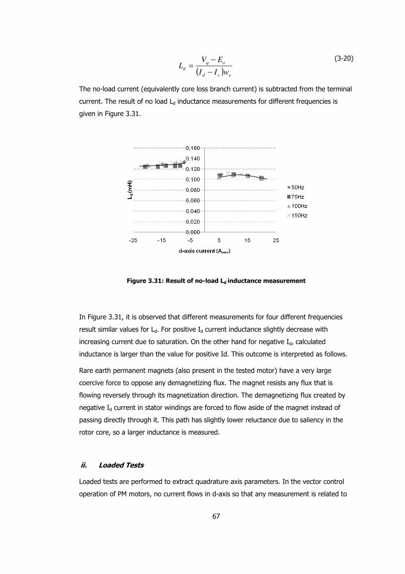
67

( ) ecd

oq

dwII

EVL

−

−=

(3-20)

The no-load current (equivalently core loss branch current) is subtracted from the terminal

current. The result of no load Ld inductance measurements for different frequencies is

given in Figure 3.31.

Figure 3.31: Result of no-load Ld inductance measurement

In Figure 3.31, it is observed that different measurements for four different frequencies

result similar values for Ld. For positive Id current inductance slightly decrease with

increasing current due to saturation. On the other hand for negative Id, calculated

inductance is larger than the value for positive Id. This outcome is interpreted as follows.

Rare earth permanent magnets (also present in the tested motor) have a very large

coercive force to oppose any demagnetizing flux. The magnet resists any flux that is

flowing reversely through its magnetization direction. The demagnetizing flux created by

negative Id current in stator windings are forced to flow aside of the magnet instead of

passing directly through it. This path has slightly lower reluctance due to saliency in the

rotor core, so a larger inductance is measured.

ii. Loaded Tests

Loaded tests are performed to extract quadrature axis parameters. In the vector control

operation of PM motors, no current flows in d-axis so that any measurement is related to

68

q-axis parameters. The aim of these tests is to establish q-axis currents so that related

parameter Lq can be investigated.

In this test, motor is driven under normal vector control where only q-axis current is

injected to the motor. The phase diagram related to this operation is presented in Figure

3.33. In the figure, we is operating electrical frequency, Vemf is back-EMF voltage, Vt is

motor phase voltage.

Figure 3.32: Phase diagram for Lq loaded test

Assuming induced EMF voltage is fixed with constant shaft speed, the voltage difference

between q-axis component of terminal voltage and calculated EMF voltage at that speed

can be resolved to inductance (Equation (3-21)).

( ) ecq

q

qwII

VL

−=

δsin

(3-21)

The no-load current (equivalently core loss branch current) is subtracted from the terminal

current. The result of no load Lq inductance measurements for different frequencies are

given in Figure 3.33.

69

0,080

0,100

0,120

0,140

0,160

0,180

0,200

0,220

0,240

0,260

0,280

0 2 4 6 8 10 12 14 16

Fundamental of Terminal Current (Arms)

Ca

lcu

late

d L

q (

mH

)

Lq 25Hz (ph.A data) Lq 25Hz (ph.B data) Lq 50Hz (ph.A data)

Lq 50Hz (ph.B data) Lq 100Hz (ph.A data) Lq 100Hz (ph.B data)

Figure 3.33: Result of loaded Lq inductance measurement for loaded running test

As observed from Figure 3.33, there is not a unique Lq value to determine from the loaded

test results. It is observed that for each frequency calculated inductance increases with

current. Toward twice of the rated current measured value stabilizes.

The expectation from the loaded test was to get a curve of Lq variation that is decreasing

monotonously by motor terminal current (due to possible saturation with increasing

current). However different trends for Lq variation are observed for different frequencies.

Discussions and probable reasons for these unexpected results will be presented in Section

3.4.

3.3.4 Result of Back EMF Voltage Measurement

The measurement was done while running the machine as a generator with open circuited

terminals. The line-to-line voltage signal was recorded using a digital oscilloscope. The

variation of back EMF voltage amplitude with speed is visualized in Figure 3.34 and one

sample of recorded waveforms is presented in Figure 3.35. The gradient of linear

approximation (slope of linear trend line) to recorded data points gives EMF voltage

constant for the motor.

70

Figure 3.34: Measured EMF voltages for different speeds

As observed in Figure 3.34, EMF voltage constant is measured as 0.070 Vpeak.s/rad at line

which is equivalent to 0.029 Vrms.s/rad per phase. A sample measured voltage waveform

showing sinusoidal back EMF at line is presented in Figure 3.35.

Figure 3.35: Measured EMF waveform at motor terminals at 1000rpm

71

3.3.5 Results of No-Load Loss Measurement

In this thesis work, two different loss measurement tests are performed. In one case,

motor is driven by an auxiliary motor and torque at shaft is measured as power input to

the tested motor. In the other case, the tested motor is operated at no load and power

input at terminal is measured.

Method.1 – Test motor driven by an auxiliary motor

In the test, the PMSM is externally coupled to a driving motor which can be operated in

variable speeds. There is a torque transducer between the driving motor and the PMSM.

When the driving motor is operated, the measured torque corresponds to total of

mechanical losses; friction and windage losses. The measurement results for the sample

motor are tabulated in Table 3.7.

Table 3.7: Measurement results for Losses by Method.1

Shaft Speed

(rpm) Operating Electrical Frequency (Hz)

Measured Torque

(Nm) Measured Power Input

(W)

172 11 0,010 0,18

325 22 0,017 0,58

630 42 0,021 1,39

745 50 0,023 1,79

974 65 0,024 2,45

1300 87 0,028 3,81

Method.2 – Test motor driven at no load by an inverter

For this test, motor is run with no-load at various speeds. The rms terminal voltage, rms

current and input power are recorded. In this operation, it is assumed that a negligible

electromagnetic torque is produced (only for friction-windage) for any speed so that

measured power input to the motor can be treated as total of friction-windage losses and

core loss. In this test, the test setup in Figure 3.2 is used without any load coupled to PM

motor. Copper losses are ignored in this test since current is very small. The measurement

results at motor terminals and calculations are presented in Table 3.8.

72

Table 3.8: Measurement results for Losses by Method.2

Shaft Speed

(rpm)

Operating Electrical

Frequency (Hz)

Motor Terminal Current (Arms)

Motor Terminal Voltage (Vrms)

Measured Input power (W)

750 50 0,31 3,95 2,12

1125 75 0,33 5,89 3,37

1500 100 0,36 7,71 4,81

2250 150 0,44 11,15 8,50

The variation of the losses by both methods is clearer in Figure 3.36 where a second order

approximation is done for calculated loss data points.

y = 0,0002x2 + 0,0333x

y = 0,0003x2 + 0,0218x

0

1

2

3

4

5

6

7

8

9

10

0 20 40 60 80 100 120 140 160 180

Operating Electrical Frequency (Hz)

Calc

ula

ted

Lo

ss a

t M

oto

r T

erm

inals

(W

)

Method.1

Method.2

Figure 3.36: Variation of no-load losses with frequency by two methods

It is observed that 0.2W larger loss is measured by Method.2 at low frequencies but

Method.1 measurements have steeper trend line which means that losses will be higher at

higher frequencies. Either of them may be selected to include in analytical calculations. In

this thesis work, results of no-load loss tests by Method.2 are selected to be used in

analytical calculations.

73

3.3.6 Results of Inductance Test by DC Current Decay

The DC decay method is presented in Section 3.2.2-iii which is proposed by Boldea [40].

The idea behind this test is that rate of current flow in a conducting medium cannot be

altered discretely in a conducting medium. Instead, the change happens in an exponential

trend with time constant. The time constant is solely dependent on total impedance of the

path.

Exciting the motor windings with DC will result in a constant current flow. Opening the

switch, blocking the current from source, induced currents in motor windings will flow

through the diode and diminish rapidly with a time-constant. If the oscilloscope is

triggered to track the decaying current, inductance can be calculated determined from the

recorded waveform.

The test bench for DC current decay can be setup by connecting the PM motor, in parallel

with a diode, to a DC source through a switch. In serial with switch-motor connection, an

oscilloscope is used for recording the terminal current.

Figure 3.37: Test setup for standstill DC current decay test

Calculation of inductance may be done in terms of preservation of energy rule. The initial

energy stored in the inductor at the time of switching will be dissipated on resistance of

the system. If resistance of the system is known then equivalent inductance of the system

may be calculated by energy balance equation.

E stored in inductor = E dissipated on resistance (3-22)

Equation (3-22) can be explicitly written as follows.

74

dtRtILI o ⋅⋅= ∫∞

0

22 )(2

1 (3-23)

For discrete time data, the expression in equation (3-23) can be rewritten as follows.

∑=

⋅⋅=N

k

ko RhILI0

22

2

1 (3-24)

The sampling time “h”, resistance “R”, initial value of the direct current “Io“ and the

current samples “Ik“ during the decay period are known.

Inductance variation by DC current is identified by repeating the measurement for

different current amplitudes and for both d-axis and q-axis. Alignment is done as proposed

in standstill AC test.

A sample DC decay current from recorded waveforms is presented in Figure 3.38. The

oscilloscope is triggered with opening of switch at time t=0.

Figure 3.38: Recorded DC decay current in d-axis DC current decay test at 20A

Inductance can be calculated by recorded data if equation (3-24) is rewritten with known

parameters.

2

0

22

o

N

k

k

I

IhR

L

∑=

⋅⋅⋅

= (3-25)

Calculated inductances by equation (3-25) from DC decay measurements are tabulated in

Table 3.9.

75

Table 3.9: Results of DC current decay

Initial current

Io (A) Sampling time h

(µsec)

Calculated Inductance

(µH)

4,48 0,2 33

9,24 0,4 52

14,10 0,4 63 q-axis

19,68 0,4 67

4,32 0,2 29

9,44 0,2 42

13,95 0,4 50 d-axis

18,56 0,4 53

Figure 3.39: DC current decay test results

3.3.7 Result of Motor Thermal Constant Measurement

The test motor is loaded with 1 Nm at 1400 rpm. Thermal equilibrium is observed after 90

minutes of operation. The temperature rise of the motor with respect to time is illustrated

in Figure 3.40.

At the defined operating condition, measurements and thermal constant calculations are

as follows:

76

Output power : 147 W (1 Nm @ 1400 rpm)

Input power : 187 W

Total loss : 40 W

Efficiency : 78%

Ambient temperature : 20 °C

Temperature rise : 80 °C

Thermal constant : 2 °C/W (80°C / 40W)

0

10

20

30

40

50

60

70

80

90

0 20 40 60 80 100

Time (min)

Te

mp

era

ture

Ris

e (

°C)

Figure 3.40: Temperature rise of tested motor under 1 Nm load at 1400 rpm

3.3.8 Result of Torque – Speed Measurement

During this test, the motor is driven at selected frequencies. At a specific frequency

(equivalently speed), the load is gradually increased until the permissible peak current (35

Arms) is reached. The value of torque recorded at that point is taken as pull-out torque at

that speed. The result is presented in Figure 3.41.

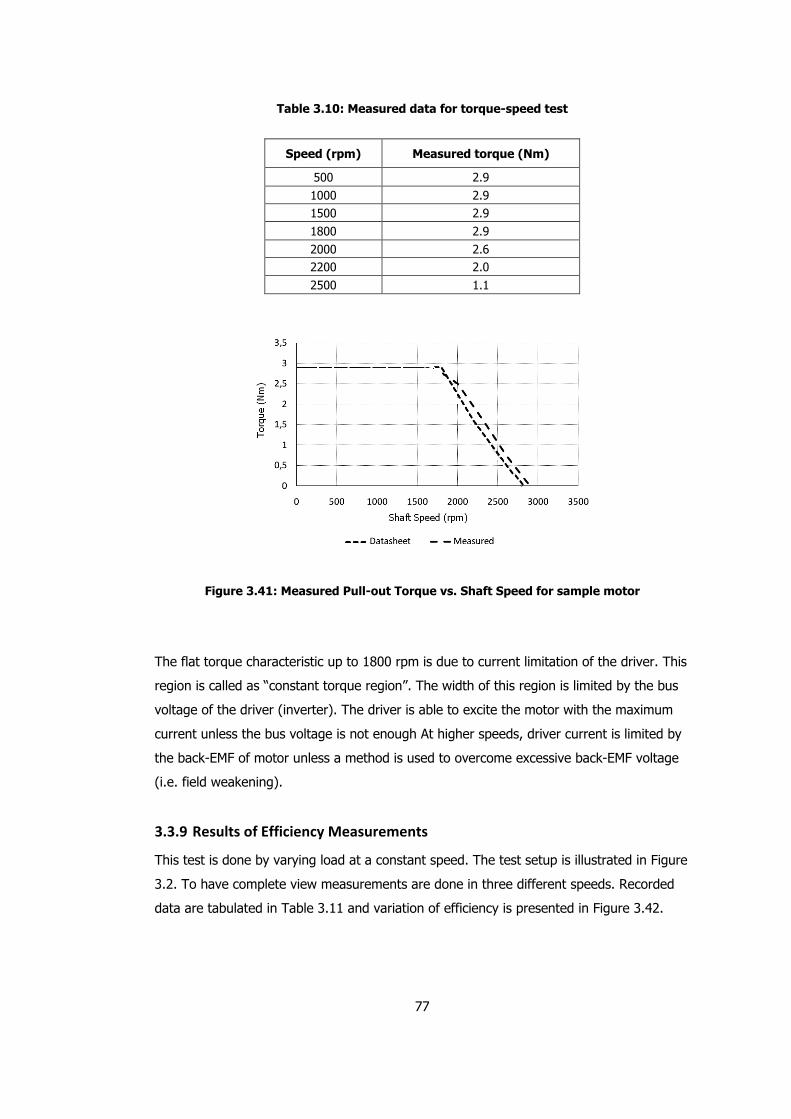
77

Table 3.10: Measured data for torque-speed test

Speed (rpm) Measured torque (Nm)

500 2.9

1000 2.9

1500 2.9

1800 2.9

2000 2.6 2200 2.0

2500 1.1

Figure 3.41: Measured Pull-out Torque vs. Shaft Speed for sample motor

The flat torque characteristic up to 1800 rpm is due to current limitation of the driver. This

region is called as “constant torque region”. The width of this region is limited by the bus

voltage of the driver (inverter). The driver is able to excite the motor with the maximum

current unless the bus voltage is not enough At higher speeds, driver current is limited by

the back-EMF of motor unless a method is used to overcome excessive back-EMF voltage

(i.e. field weakening).

3.3.9 Results of Efficiency Measurements

This test is done by varying load at a constant speed. The test setup is illustrated in Figure

3.2. To have complete view measurements are done in three different speeds. Recorded

data are tabulated in Table 3.11 and variation of efficiency is presented in Figure 3.42.

78

Figure 3.42: Sample motor efficiency vs. shaft load at constant speed

Table 3.11: Measured efficiency test data

Speed (rpm)

Terminal Current (Arms)

Input Power (W)

Input Power Factor

Motor Output Power (W)

Efficiency (%)

5,70 33,26 1,00 25,6 77

11,04 78,01 0,99 49,7 64

16,00 132,08 0,98 72,0 55

20,77 198,4 0,98 93,5 47

500

25,36 277,38 0,98 114,2 41

5,78 60,88 1,00 52,1 86

11,10 129,61 0,99 99,9 77

15,84 201,10 0,99 142,6 71

20,72 290,40 0,98 186,6 64

1000

25,76 402,92 0,97 232,0 58

5,25 79,83 1,00 70,9 89

11,09 180,47 0,99 149,8 83

16,00 281,38 0,99 216,2 77

20,97 397,20 0,98 283,5 71

1500

26,12 515,98 0,97 352,9 68

It is an expected result that efficiency is better for higher speeds. The major loss in PM

machines is copper loss. Since the machine gives same torque output at same current

levels for different speeds, copper losses stays same as the output power increases. So

losses become less dominant and efficiency is calculated to be higher.

3.3.10 Results of Cogging Torque Measurement

The frequency of this torque depends on number of poles on rotor and number of teeth in

stator. It is expected to see cogging torque at multiples of pole number, stator number

and minimum common multiple of them [7]. For the tested sample motor which has 8 poles

and 27 slots, cogging torque is expected at 8, 27 and 8*27 multiples of shaft rotational

frequency.

79

In this thesis work, a 90L frame 1.1kW induction motor was used to drive the test motor

assuming that the inertia will be enough to keep the speed constant.

Figure 3.43: Cogging torque measurement test setup

Torque on the shaft is measured at different speeds ranging from 60 rpm to 563 rpm to

observe the effect of shaft speed to cogging torque measurements. Shaft speed and

torque is measured by transducer and displayed on a two-channel oscilloscope which

records this waveform also. FFT analysis applied to measured torque waveform to

investigate different harmonic components of torque. At each measurement, harmonic

components with amplitude less than 1% of highest component are ignored.

From the measurements, following interpretations can be done:

i. The DC torque component in the measurements about 4.5 Ncm is interpreted as

friction.

ii. It was expected to observe torque components at 8, 27 and 8*27 times shaft

frequency but it is not possible to identify those from the measurements.

Measured torque values at sub-frequencies are all lower than 0.002 Nm.

iii. As the speed increases, torque harmonics at supply frequency diminish.

80

Table 3.12: Measured torque data for cogging torque test

Speed: 60 rpm, fm = 1 Hz, Speed fluctuation: 1.2rpm (±0.02Hz)

Frequency Component

DC fm 6fm 7,5fm

Measured Moment (Ncm)

4,77 0,1 0,2 0,1

Speed: 141.6rpm, fm = 2.36Hz, Speed fluctuation: 1.8rpm (±0.03Hz)

Frequency Component

DC fm 6fm 7,5fm


4,7

Speed: 282rpm, fm = 4.7Hz, Speed fluctuation: 1.8rpm (±0.03Hz)

Frequency Component

DC fm 2fm 7,5fm


4,59 0,05 0,16

Speed: 420rpm, fm = 7Hz, Speed fluctuation: 0rpm

Frequency Component

DC fm-1 fm fm+1 2fm-1 2fm 2fm+1


4 0,06 - 0,15 0,04 0,125 0,08

Speed: 564rpm, fm: 9.4Hz, Speed fluctuation: 0rpm

Frequency Component

DC fm-1 fm fm+1 2fm-1 2fm 2fm+1


4,14 0,088 0,122

The cogging torque of sample motor is also analyzed by FE analysis with Maxwell and

Flux2D. In Maxwell, cogging torque is determined as 0.002 Nm peak whereas in Flux2D as

0.0018 Nm peak. Resultant waveforms are presented in Figure 3.44, Figure 3.45.

Figure 3.44: Cogging torque analysis results by Maxwell

81

Figure 3.45: Cogging torque analysis results by Flux2D

3.4 Comparison of Inductance Measurements and Discussions

In this section results of different inductance measurements tests are discussed. The

purpose is to investigate and compare results of the proposed methods and conclude

which ones are most applicable.

3.4.1 Direct-Axis Inductance Ld Measurements

a.) Comparison of measurements at Standstill

The results of standstill tests are presented in Section 3.3.2. Following comments can be

made regarding to results:

Measured Ld from AC sinusoidal excitation tests is around 115 uH and has a

decreasing trend with 1% slope up to rated current.

Measured Ld from PWM excitation tests is around 115 uH and has an increasing

trend with 1% slope up to rated current.

Both standstill results are independent of test frequency (same Ld values for

25Hz, 50Hz, 100Hz).

Measured Ld values from DC decay tests do not give comparable results with

other tests. The measured value is around 29 uH at 5Adc. Ld variation has an

increasing trend up to rated current where measured value reaches 50 uH.

82

b.) Comparison of Running test results with standstill tests

Measured Ld from running no-load tests is within the bound 105 uH…110 uH up

to rated current.

Measured Ld values is within 3% for different test frequencies.

Since standstill tests also give Ld value of 110 uH, it can be concluded that no-

load running tests and standstill tests agree with each other.

c.) Comparison under demagnetizing conditions

Ld tests under demagnetizing conditions are performed only in no-load running

tests because in standstill tests, the magnets subjected to variable flux which

realizes magnetizing and demagnetizing conditions at the same time.

Measured Ld from running tests is larger than magnetizing conditions. This

outcome is interpreted as follows. Weakening of magnet flux decreases flux level in

stator steel so that any present saturations in flux paths diminishes. This results in

increased inductance value.

3.4.2 Quadrature-Axis Inductance Lq Measurements

a.) Comparison of measurements at Standstill

Measured Lq from AC sinusoidal excitation tests is around 130…133 uH and has

a decreasing trend to 130 uH with 1% slope up to rated current.

Measured Lq from PWM excitation tests is around 132 uH and has an increasing

trend to 133 uH with 1% slope up to rated current.

Measured Lq from DC decay tests do not give comparable results with standstill

excitation tests. The measured value is around 33 uH at 5Adc. Lq variation has an

increasing trend up to rated current where measured value reaches 67 uH.

b.) Comparison of Running test results with standstill tests

It is observed in loaded q-axis inductance tests that measured Lq values are very

diverse for different frequencies and currents. Measured Lq values from running

tests spread over a wide range.

It is not possible to comment on the exact value of inductance from measured

results. A single Lq value can not be defined even for the same current and

frequency for load test which questions the accuracy and reliability of the

measurement.

83

Scattering of Lq values decreases with higher current (equivalently load).

3.4.3 Result of Inductance Measurements

For each axis inductance (Ld, Lq), four different measurements (Standstill AC test,

Standstill PWM test, DC current decay test, Running load test) are made and also each

measurement is validated by FE analyses. A comparison of the inductances obtained by

measurements proposed methods are tabulated in Table 3.13, Table 3.14 and Table 3.15.

To be able to compare results of different measurements, all given data in the tables is for

the same current level.

Table 3.13: Inductance measurement results for different methods at 5 Arms

Fundamental of Terminal current: 5 Arms

Measurement Method

d-axis Inductance

Ld (mH)

(25 Hz / 50 Hz / 100 Hz)

q-axis Inductance

Lq (mH)

(25 Hz / 50 Hz / 100 Hz)

Manufacturer data 0.125 0.133

Standstill AC Test

(Sinusoidal voltage excitation) 0.113 / 0.113 / 0.114 0.129 / 0.130 / 0.132

Standstill AC Test

(PWM voltage excitation) 0.115 / 0.114 / 0.114 0.131 / 0.132 / 0.132

Running No-Load Test 0.104 / 0.108 / 0.110 -

Running Load Test - 0.130~0.230 / 0.195~0.250 /

0.240~0.260

DC Decay 0.029 0.033

Both load tests and dc decay test results are not consistent with theory which states that

inductance may decrease with increasing current due to saturation. It can be concluded

that standstill tests give satisfactory and reliable results where as it is not possible to state

this for running and dc decay tests. In the following sections, possible reasons for

inaccuracy in load tests are tried to be defined.

84



Measurement Method

d-axis Inductance

Ld (mH)

(25 Hz / 50 Hz / 100 Hz)

q-axis Inductance

Lq (mH)

(25 Hz / 50 Hz / 100 Hz)


Standstill AC Test

(Sinusoidal voltage excitation) 0.114 / 0.114 / 0.114 0.129 / 0.130 / 0.135

Standstill AC Test



Running Load Test - 0.106~0.155 / 0.132~0.156 /

0.189~0.200

DC Decay 0.042 0.052



Measurement Method

d-axis Inductance

Ld (mH)

(25 Hz / 50 Hz / 100 Hz)

q-axis Inductance

Lq (mH)

(25 Hz / 50 Hz / 100 Hz)


Standstill AC Test

(Sinusoidal voltage excitation)

0.119 (only data for 50Hz)

0.130 (only data for 50Hz)

Standstill AC Test



Running Load Test - 0.091~0.114 / 0.130~0.160 / no

data for 100Hz

DC Decay 0.050 0.063

Dependency of Inductance measurements to Load Angle

The determination of load angle is critical if running tests are performed for parameters

measurements. To have a solvable equation set of motor model (equations (2-5) and

(2-6)) either the load angle must be determined accurately in some manner or another set

of equations based on some assumptions have to be developed.

The accuracy of the determined load angle with decreasing load (equivalently lower motor

terminal current) since load angle is proportional to load. It may be very small at light

85

loads (around 5° electrical). In this situation any miscalculation may lead to large variation

of load angle. To understand the dependence of measured load angle and calculated

inductance, a fictitious derivation is made as follows:

Say that in a specific loading condition (which is probable where the PM machine is

loaded below rated conditions) the machine operating with a load angle of 5

degrees electrical. Also assume that the load angle is measured exactly. In q-axis

running tests, the amplitude of fundamental harmonic of terminal voltage is

multiplied by sin δ to calculate voltage induced on q-axis inductance (Figure 3.29).

( ) 087.05sin =°=δ (3-26)

If the determined load angle was measured within ±1° error:

( ) 070.04sin =°=δ (3-27)

( ) 104.06sin =°=δ (3-28)

It is obvious that a ±1° (20%) error in angle measurement (which is very probable in case

of such small angles) dramatically affects inductance calculation. If studied load angle was

larger (around 20° as in standstill test measurements, see presented results in Section

3.3.2), a measurement error would not be so effective. However as the load angle

becomes smaller, a linear relation is observed with angle error and calculated inductance.

Some recorded phase angles during q-axis running test at 50 Hz is tabulated in Table 3.16

for three different terminal currents. Many measurements are done to specify the variation

of the recorded angle.

Table 3.16: Measured phase angles at different currents

Motor Terminal

Current (Arms) Measured Phase Angles

Variation of measured

values

6.2

3,09 / 3 / 2,96 / 2,83 / 2 / 1,93

2,88 / 2,82 / 2,94 / 2,89 / 2,85

1,93 / 3,08 / 3,04 / 2,18 / 2,63

2,7 / 3,09 / 3,68 / 2,07 / 2,77

±30%

10.8

4,69 / 4,81 / 4,64 / 5,1 / 4,62 / 4,77

4,92 / 4,82 / 4,76 / 4,63 / 4,64 / 4,77 / 4,58 / 4,93 / 4,77 / 5,01 / 4,85 / 4,9 / 5 / 5,03 /

4,09

±5%

15 6,88 / 7,17 / 6,94 / 7,17 / 6,8 / 7,21

6,83 / 6,94 / 6,93 / 6,88 / 7,06 ±3%

86

It is observed in Table 3.16 that as the measured phase angle gets smaller, scattering of

measured phase angle becomes larger; or equivalently as the terminal current decreases

the uncertainty in measured phase angle increases. Consequently, for this range of phase

angle (equivalently load angle), calculations of inductance based on measurements

become unreliable.

Sine value of load angle is plotted with respect to current for different frequencies in

Figure 3.46. It is observed that, although frequency becomes 8 times larger, sine of load

angle is only 2 times at maximum current.

0,000

0,050

0,100

0,150

0,200

0,250

0,300

0,350

0,400

0,450

0,500

0 5 10 15 20 25 30 35 40

Motor Phase Current (Arms)

Ca

lcu

late

d S

ine

of

Th

eo

reti

ca

l L

oa

d A

ng

le

25 Hz 50 Hz 100 Hz 200 Hz

Figure 3.46: Value of sine of load angle for different frequencies and currents

Dependency of Measurements to Vector Control

As stated before, a vector controlled drive is used in the tests. It is assumed that vector

control satisfies Id=0 condition where Iq becomes completely in phase with back EFM

voltage Eo (Figure 3.47).

87

Figure 3.47: Phase diagram of PMSM for vector control

It is evident that exact real time control can not be achieved even for simple digital

circuits. There is always a delay time between successive control steps due to process

time. In today’s drive applications generally 150 µsec passes to close a control loop (e.g.

speed loop) and apply the vector excitation to motor terminals. This states that during 150

µsec time no feedback comes from motor and control is lost. Id=0 case may be valid for

the instant of applied excitation however for the next 150 µsec the applied excitation can

not satisfy Id=0 condition. The error in such a condition can be checked easily as follows.

Let’s assume that motor is operated at 1500rpm. It must be noted that the tested motor

has four pole pairs which results in four times 360 electrical degrees in one mechanical

revolution. At this speed, rotor completes one mechanical revolution at 40 µsec. Four

times 360 degrees is spanned in 40 µsec. We stated that one control loop lasts 150 µsec.

The angular rotation of rotor in this period can be calculated as;

°=° 4.5360440

15.0xx (3-29)

It is clear that a vector control drive with 150 µsec control loop time has a maximum of

5.4° angle error in vector control. This means that terminal current vector I may be out of

phase with back EMF voltage Eo by 5.4° where Id=0 can not be satisfied.

Since all the calculations in running tests rely on Id=0 condition to be satisfied, all

inductance calculations are completely distributed over an error range. The observed

distributed inductance values in load tests in Figure 3.33 results from this situation.

Running tests has a fixed error range regarding to vector control loop time. It is shown in

88

previous section that such an angle error results in calculation errors by 100% which

questions reliability and accuracy of inductance values measured by load tests.

Dependency of Measurements on Test Frequency

In presented results in section 3.3.3 that calculated inductance values vary by operating

frequency. As stated before, this is completely contradictory with theory which states

inductance is a function of flux created per unit of a current, no relation to frequency is

present. This result may be an outcome of vector control error stated in section 0.

On the other hand, Senjyu et. al. [32] had a similar result which shows lower inductance for

higher frequencies (Figure 3.48).

Figure 3.48: Result of inductance measurement by Senjyu [32]

This does not state that inductance may vary with frequency; however it is useful to show

that variations with frequency may be observed due to possible load angle measurement

errors.

Dependency of Measurements to Harmonic Elimination

Most of modern motor drive systems have a PWM output voltage to supply currents to

motor terminals. The voltage waveform at motor terminals is highly distorted and far from

sinusoidal shape. In inductance calculations, the fundamental harmonic components of

voltages and currents are used since phase diagrams modelling the motor is constructed

based on fundamental quantities.

89

For a PWM voltage waveform, the extraction of fundamental component both affects

amplitude and phase which are two main parameters in inductance calculation.

Inaccuracies in harmonic directly affect the calculated inductance. For example, a 5%

error in amplitude of voltage fundamental will result in 5% error in calculated inductance.

With other probable measurement inaccuracies, this error may establish a result far from

reality.

The consistency between calculated inductance values for AC excitation and PWM shows

that fundamental components of both voltage and current are correctly extracted with the

harmonic analyzer used in the test setup. It can assumed that harmonic extraction can be

performed reliably with a harmonic analyzer; so a PWM waveform can not be (or the last)

a cause for unreliable distributed inductance values observed in load tests.

3.5 Discussions on Measurements

In section 3.3, selected test methods from the proposed tests in Section 3.2 are performed

on the tested motor. Following conclusions can be made regarding to measurement

results.

Winding resistance can be measured precisely with four-wired setup as

described in 3.2.1. The measured value at room temperature must be modified at

higher temperatures. A 100°C can result in 35% increase in actual resistance as

mathematically expressed in (3-1).

Inductance measurement is a challenging issue, especially measurement of Lq.

Standstill measurements with AC or PWM excitation give reliable results for both Ld

and Lq measurements.

Running no-load test for Ld gives accurate results for different frequencies and

current values. The reason for that is, load angle is small in this tests and cosine of

load angle δ is used in calculations. This result in reliable measurements which are

not very sensitive to load angle errors.

Running load test for Lq gives scattered inductance values on the current and

frequency range. Since sine function of load angle is used in the calculations,

calculated inductance value is very sensitive to load angle. Vector control loop also

introduces a load angle error naturally due to control in discrete times (e.g. every

150 µsec).

The sensitivity of Lq measurement to load angle may be reduced by performing

the test at specific conditions where load angle is big and angle errors introduced by

vector control is low. This condition can be satisfied by performing the test at low

90

speed with high load where vector control loop is fast enough to realize Id=0

condition and motor current is high enough to have a large “Iq.Xq” vector on the

phase diagram. This comment can be validated by observing load angle variation

with respect to frequency and load. The variation of sine value of load angle is

plotted in Figure 3.46. It can be observed that load angle sine value at 200 Hz at

maximum current becomes 2.5 times although frequency is increased 8 times from

25 Hz to 200 Hz.

Back-emf voltage measurement of PM machine is easy to conduct. As long as

the tested motor is driven by auxiliary means at a speed, generated can be

observed at motor terminals. The emf – speed relation is expected to have a linear

relation between. An extra but useful effort may be to perform emf test at different

ambient temperatures to extract temperature dependence of back emf. This kind of

test can be conducted in a temperature chamber.

It is shown in Section 3.2.4 that friction-windage losses can not be separated

from core loss in PM machines. Rotor magnets have to be removed to measure only

friction-windage loss which requires disassembling of the motor.

Torque-Speed measurement has a straight forward procedure which is described

in 3.2.5. As observed in Figure 3.41, measurements are consistent with

manufacturer data.

Motor efficiency test can be performed as described in Section 3.2.7. During the

test, it wise to record motor temperature also beside electrical measurements.

It is better to perform cogging torque measurements at very low speed with

high inertia. This is also suggested by Boldea [40]. Test at low speed enhances the

torque accuracy and high inertia assists keeping the shaft speed constant while

driving the test motor by auxiliary means.

91

CHAPTER 4

ANALYTICAL CALCULATION of

BRUSHLESS DC MOTOR PARAMETERS and PERFORMANCE

In this chapter, mathematical equations related to the parameters in the magnetic and

electrical model of an inset-magnet PM motor is going to be derived in terms of motor

dimensions and some other parameters. The ultimate goal is to develop a mathematical

model which can be used to analytically estimate the performance of a radial flux inset-

magnet electrical machine from its geometry and material properties.

Mechanical dimensions and material properties in the machine will be used as an input the

model. The outcomes are values of the parameters in the machine model and performance

characteristics like torque-speed, power-speed etc.

The equations will be derived in terms of designated names like “L” for axial length of steel

core and “Br” for magnet remanent flux density to get a generalized view. At the end of

this chapter, the verification of the derived mathematical model will be done with an

available PM motor which is fully characterized by performance tests, parameter

measurements and dimensional measurements on the disassembled mechanical body. The

measurement results are presented in CHAPTER 3 and abbreviations for mechanical

dimensions are illustrated in Figure 4.1.

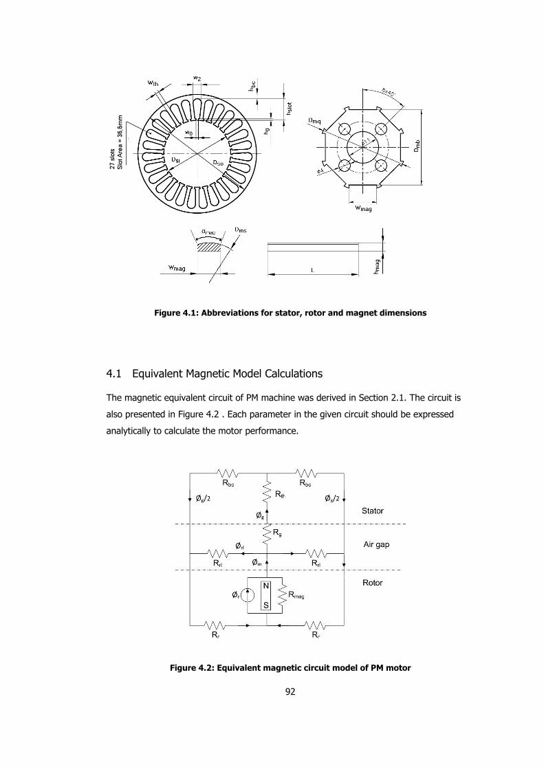
92

Figure 4.1: Abbreviations for stator, rotor and magnet dimensions

4.1 Equivalent Magnetic Model Calculations

The magnetic equivalent circuit of PM machine was derived in Section 2.1. The circuit is

also presented in Figure 4.2 . Each parameter in the given circuit should be expressed

analytically to calculate the motor performance.

Figure 4.2: Equivalent magnetic circuit model of PM motor

93

The parameters in the equivalent circuit are defined as follows. Definitions of the variables

may be found in Chapter 2.

Ør : Flux generated by magnet

Øm : Flux leaving magnet and passing to airgap

Ørl : Rotor leakage flux between poles (through Rrl)

Øg : Flux at airgap passing from rotor to stator side

Rmag : Magnet internal leakage path reluctance

Rrl : Reluctance of leakage path between magnets

Rg : Equivalent airgap magnetic reluctance Rth : Equivalent tooth magnetic reluctance Rbc : Equivalent back core magnetic reluctance Rr : Reluctance of rotor yoke

4.1.1 Magnet Flux and Reluctances

The process of obtaining analytical expressions of the parameters is started with modelling

the magnet. In the magnetic equivalent model, the magnet is modelled with a flux source

Ør in parallel with leakage reluctance Rmag which is Norton equivalent model. This method

is also used in electrical circuit analysis for voltage sources. Norton equivalent of the

magnet can be expressed as follows.

magr AB=0φ (4-1)

magr

mag

magA

hR

0µµ= (4-2)

In the equations (4-1) and (4-2), Br is remanent flux density of the magnet which is defined

by the magnet manufacturer and it is temperature dependent, Amag is cross sectional area

of the magnet in normal direction to magnetization direction, hmag is magnet length in

magnetization direction, µr and µo are magnet relative recoil and free space permeabilities

respectively. Magnet cross sectional area “Amag” is calculated by multiplying magnet width

“Wmag” with axial length L (Figure 4.3).

LWA magmag = (4-3)

94

Figure 4.3: Defined dimensions of a cubic magnet

(Arrows show magnetization direction)

For simple shaped magnets like in Figure 4.3, reluctance expression given in equation (4-2)

is useful. However for most machine designs, magnets have special shapes to get a

sinusoidal flux distribution in the air gap. In such case, it is wise to split the magnet along

the magnetization direction into smaller pieces, calculate reluctance for each piece and

then treat them as in parallel to get total reluctance. In this work, the magnet is shaped as

shown in Fig. 4.4 It is split into five pieces as seen in Figure 4.4.

Figure 4.4: Illustration of magnet reluctance derivation

In the above figure, reluctances are assigned for each magnet piece. However it should be

noted that since pieces 2 & 4 and 1 & 5 are identical due to symmetry, same reluctances

are assigned for them in pairs. The total reluctance of the magnet can be obtained from

equation (4-4).

1

321

122−

++=

magmagmag

magRRR

R (4-4)

95

Since magnet is sliced into 5 equal width pieces, cross sectional area in equation (4-1)

must be taken as Amag /5 to calculate reluctance for each. Also it must be noted that hmag is

different for each piece. To calculate height of each magnet piece, some geometrical

derivation must be faced.

1

321

0

1

0

3

0

2

0

1

1

321

122

5

1

5

1

5

2

5

2

122

−

−

−

++=

++=

++=

magmagmagmag

r

mag

r

mag

mag

r

mag

mag

r

mag

magmagmag

mag

hhhL

W

LW

h

LW

h

LW

h

RRRR

µµ

µµµµµµ

(4-5)

−

×= mbmagmsmag DDh α

5

2cos5.01

(4-6)

−

×= mbmagmsmag DDh α

5

1cos5.02

(4-7)

( )mbmsmbmagmsmag DDDDh −×=

−

×= 5.0

5

0cos5.03 α

(4-8)

×= −

ms

mag

magD

W1sin2α

(4-9)

In the equations (4-5)-(4-9), hmag1-2-3 are height of each magnet region as defined in Figure

4.4, Dms, Dmb, Wmag are illustrated in Figure 4.1, θmag is angle span of magnet surface in

mechanical degrees. To be more clear, a magnet having a 2/3 pole pitch in 8 pole motor

has 30° angle span (equation (4-10)).

o308

360

3

2=×=magθ (4-10)

4.1.2 Rotor Leakage Reluctance

This parameter represents the path for flux which does not pass from magnet to stator but

instead leak from one magnet to adjacent one. As Miller [6] stated, it is hard to define

leakage paths but instead they can be assigned a value as a portion of magnet reluctance

96

and Rrl is expected to be 5-20% of magnet reluctance Rmag. The effect of leakage

reluctance on airgap magnetic flux density results in 0,005Nm torque calculation error.

Considering the rated torque of the sample motor (1,47Nm), this error is acceptable. In

conclude, Rrl is going to be defined as “10*Rmag”.

magrl RR ×= 10 (4-11)

4.1.3 Airgap Reluctance

The airgap reluctance is perhaps the most important parameter in the equivalent magnetic

circuit, since to determine airgap flux, airgap reluctance must be defined. Also this

parameter determines the magnetizing inductance of a motor. The general expression for

airgap reluctance is given by

gap

gA

gR

0µ

′= (4-12)

where Agap is the pole pitch area midway along flux direction between stator inner surface

and magnet surface. “g’” is modified airgap g with Carter’s coefficient kc to include effect

of stator slotting on airgap flux density. Airgap is modified as in equation (4-13).

ckgg ⋅=′ (4-13)

Derivation of Carter Coefficient is presented by F.W. Carter [41] as in equation (4-14).

g

kc

500/0

2

00/0

1/0

00/0

00/0

+−

=

ω

ωλ

λ

(4-14)

In the equation, the subscript “0” refers to stator side whereas “00” refers to rotor side.

Respective dimensions should be selected to calculate Carter’s coefficient for stator or

rotor side. Dimensions of stator and rotor surface structure are defined as in Figure 4.5 for

the tested sample motor.

97

Figure 4.5: Abbreviations for stator and rotor surface dimensions for Carter’s coefficient

calculation

In the figure; “g” is airgap, “w0” is stator slot opening width, “w00” displacement between

rotor magnets, “λ0” is stator slot pitch, “λ00” is rotor pole pitch calculated at radius

tangential to magnet surface tip. Carter coefficient for stator side “kc0” can be calculated

as in equation (4-15).

gND

NDk

slotsi

slotsi

c

5/

/

0

2

0

0

+−

=

ω

ωπ

π

(4-15)

The airgap area (Figure 4.6) is defined as the cross sectional area of the path that the flux

follows while passing from magnet to stator (or vice versa). The flux path in the airgap is

dominantly set up by the magnetization direction of the magnet. However some fringing

flux inevitably exists in the airgap. The area seen by the flux increases with the fringing

flux. Exact area may not be defined easily but an acceptable approximation can be made.

In Figure 4.6, flux passing from magnet to stator is shown by arrows. The shaded areas at

two sides of the magnet point to fringing flux. The width of each fringing area is

approximated as equal to airgap depth “g” [6], so area of total region seen by flux can be

evaluated as in equation (4-16) by adding two times airgap to magnet surface width.

LgDA magmsgap ×

+= 2

2

1α (4-16)

In the equation “Dms” is diameter of roundness of magnet surface and “αmag” is angular

span of magnet defined in Figure 4.1.

98

Figure 4.6: Fringing flux in the airgap

(Arrows show flux direction)

To calculate total airgap reluctance equation (4-12) may be used with modified flux region

width.

LgD

kgR

magms

c

g

⋅

+

⋅=

22

10 αµ

(4-17)

4.1.4 Stator Tooth and Back-core Reluctance

The stator teeth and back core can be often assumed to be infinitely permeable and their

reluctance may be neglected. However, for high field density motors such as servo

applications, motor volume is forced to be minimized by pushing flux densities to

saturation level. In such cases there can be considerable amount of mmf drop on tooth

and back core path, so reluctances for these paths should be included in magnetic field

calculations. Equation (4-12) can be modified to calculate teeth and back core path

reluctances.

areationalcrosspathflux

lengthpathfluxR

steel sec0 ⋅⋅=

µµ (4-18)

( )( ) pitch

thsteel

th SLw

hhhR /

0

210

µµ

++= (4-19)

99

( )( )Lh

phDR

bcsteel

bcso

bc

0

/

µµ

π −⋅= (4-20)

In the above equations, “h0+h1+h2” defines length of path from tooth tip to slot dip, Ns/p

is number of slots per pole, L is axial length of steel core. The path for back core

reluctance is chosen to be in the middle of back core depth. Therefore the diameter of the

path at is defined as (Dso-hbc).

Figure 4.7: Abbreviations for slot dimensions

4.1.5 Solving Magnetic Circuit

In previous sections, parameters in the magnetic equivalent circuit have been derived.

Flux densities in the magnetic circuit can be determined now by solving the magnetic

circuit. Magneto motive force (MMF) created by the magnet equals to total MMF drop in

the magnetic circuit. It is going to be assumed that the MMF drop in the steel core is

insignificant with respect to MMF drop in airgap. The validation of this assumption is

shown mathematically in section 4.4.1 by equations (4-92), (4-93) and (4-94) such that

airgap reluctance is 1000 times of stator rotor and back core reluctances. MMF equation

related to magnetic circuit can be written as in equation (4-21).

( ) ( )rlmaggrm RRF +×−= φφ (4-21)

( ) ( )rlmaggr RR +×− φφ gg R⋅= φ (4-22)

magg

r

gRR /1 +

=φ

φ (4-23)

Considering rotor leakage path, magnet operating flux density can be calculated as

follows.

100

r

magg

rlg

m BRR

RRB

/1

/1

+

+= (4-24)

Airgap flux density can be calculated as follows.

magg

magr

ggRR

ABAB

/1 += (4-25)

r

magg

gmag

g BRR

AAB

/1

/

+= (4-26)

Calculated flux density Bg is present only in “Dms*αmag+2g” pole region as presented in

Figure 4.6. Airgap mean flux density is calculated as follows:

( ) g

si

magms

g BpgD

gD

B ×−

+

=/

22

1

π

α

(4-27)

Tooth flux density can be calculated assuming that all airgap flux passes to stator teeth. It

is assumed that all flux in one slot pitch links one tooth so that peak flux density in airgap

can be scaled to determine peak tooth flux density. Peak flux density can be calculated as

in equation (4-28).

r

rmag

mag

g Bgh

hB

µ+=ˆ (4-28)

Maximum tooth flux density occurs when this calculated peak flux in one slot pitch λth links

one slot.

r

th

ssi

rmag

mag

th

th

gth Bw

ND

gh

h

wBB

/ˆ π

µ

λ

+== (4-29)

Back core flux density can be calculated assuming that half of total pole flux passes

through back core.

ggbcbc ABAB2

1= (4-30)

Lh

AB

Bbc

gg

bc

2

1

= (4-31)

101

At this point, every parameter and flux density in magnetic equivalent circuit is expressed

analytically in terms of magnetic circuit dimensions. The next step is obtaining expression

for the electrical circuit parameters.

4.2 Equivalent Electrical Model Calculations

The magnetic equivalent circuit of PM machine was derived in Chapter 2.2. To be a

reminder, the equivalent electrical model circuit is also presented in Figure 4.8. Each

parameter in the given circuit should be derived analytically to build the complete

analytical model.

Figure 4.8: Two axes electrical model of PM motor

The given electrical circuit will be solved for vector control operation. The phase diagram

for this specific condition is given in Figure 3.29. That phase diagram shows that no Id

current is present in the motor that means only q-axis circuit is active.

4.2.1 Stator Winding Phase Resistance

The resistance of a conductor is calculated with following equation;

c

c

A

LR ρ= (4-32)

where “ρ” is conductor resistivity in ohm.m units, “Lc” is total conductor length in meters

and “Ac” is cross sectional area of the conductor in m2. The conductor cross sectional area

A is dependent on slot fill factor and winding scheme; single layer or double layer.

102

i. Wire cross-sectional area

Assuming that the wire conductor is selected with diameter Dwire, wire cross sectional area

can be calculated as;

4/2

wirewire DA π= (4-33)

If coil wire is not known, it can be calculated by slot area Aslot, copper fill factor kfill and

turns per coil Nt by equation (4-34).

t

fillslot

wireN

kAA

⋅⋅=

5.0 (4-34)

ii. Conductor length in one coil

The conductor length in one coil can be approximately calculated with steel core

dimensions.

( )[ ]( )π⋅+⋅++= slotsislotpitchexttwire hDNSLLNL /2 (4-35)

Nt : Turns per coil L : Steel core axial length Lext : Extension of end winding from stator Spitch : Number of slots between two conductors of a coil Nslot : Total number of slots Dsi : Diameter at stator inner surface hslot : Total depth of a slot

In equation (4-35), “Lext” defines end winding height from the stator steel. The extension is

visualized in Figure 4.12 in section 4.2.2. Its value is totally up to winding workmanship.

Similar motors have been investigated to define this length as 15mm. The expression in

parenthesis in equation (4-35) is related to one conductor side of a coil. To calculate total

length, there is a multiplication by 2.

iii. Length of conductor for connecting phase coils in series

There is also a wire connection between coils in a phase. Their resistance has to be

included in resistance calculation also. In this work, length of connection between two

adjacent coils is assumed to be equal to the length of coil end winding wc1 (Figure 4.12).

103

Figure 4.9: Connection between two adjacent coils

As shown in Figure 4.9, coil.A and coil.B are electrically connected as an example. The

length of connection wire between A- and B+ terminals of two coils is assumed to be

equal to length between two conductors of same coil (“wc1” in Figure 4.12). The length of

connection wires can vary in a single phase, but it is observed in the sample motor that

total length of connections can be approximated by multiplying coil number with single coil

end winding. With this assumption, total length of coil connections can be calculated with

equation (4-36).

( )πslotso

slot

pitchcoil

con hDN

SNL −= (4-36)

where Ncoil is found by dividing slot number by number of phase.

3

slotcoil

NN = (4-37)

Total phase resistance can be calculating by rewriting equation (4-32).

( )

wire

conwirecoil

A

LLNR

+⋅= −81068.1 (Ω) (4-38)

It must be remembered that this calculated resistance is valid for room temperatures

(25°C). The calculated value must be modified to include temperature effect by

255.234

5.234

+

+×=′

TRR (Ω) (4-39)

where R is calculated value at room temperature and R' is resistance at temperature T .

104

4.2.2 Inductance Calculation

In this section, expressions for d-q axes inductances Ld and Lq are going to be obtained in

terms of motor dimensions. In the derivation, magnetic saturation is ignored.

Total inductance of a winding has following sub-components [9].

i. Slot leakage inductance

ii. End-winding leakage inductance

iii. Magnetizing inductance

In the following sub-sections, those leakage parameters are derived.

i. Slot Leakage Inductance

Slot leakage is the due to the flux crossing the slot opening and linking the conductors in

that slot (Figure 4.10).In case the motor has a double layer winding, there are two

components of slot leakage.

- Self leakage of each coil conductor

- Mutual leakage between coils

Slot leakage inductance can be calculated by adding Lsls - Slot leakages due to each coil in

a slot and Lslm - Mutual leakage inductance between coils. It is assumed that all coils in a

phase are serially connected.

slmslsslot LLL += (4-40)

The sample motor in this thesis work is 8-pole motor and has 27 slots for 3 phase winding.

Since total number of slots per pole per phase is 1.125, there has to be double layer

winding which must be considered in leakage calculations. The leakage terms for each coil

conductor in one slot have to be calculated separately. Obviously the leakage of the

conductor in slot dip is not equal to leakage of conductor located near to slot opening.

Considering all these facts, the slot leakage terms Lsls and Lslm for a double-layer winding

can be calculated with slot dimensions by following equations [9].

( )( )2323 2

−⋅⋅++= pitch

slot

sls CpTBpBpTN

LNL (4-41)

( )pitch

slot

slm CpTBN

LNL −⋅= 13

3 2

(4-42)

105

N : Total number of turns per phase L : Steel core axial length Nslot : Total number of slots pT, pB, pTB : Specific Slot Permeance Coefficients Cpitch : Coil pitch – Ratio of angular span of a coil to one pole.

Specific slot permeances defined in (4-41) and (4-42) are related to magnetic structure on

leakage flux paths. The leakage flux due to top layer conductor travels a different path

than leakage flux due to bottom layer conductor. Also there is a mutual flux path due to

interaction of top and bottom layer winding (Figure 4.10).

Figure 4.10: Contours showing slot leakage paths

In Figure 4.10, double layer winding is shown by two conductors and there are three

contours of leakage flux path. Each path has its own inductance which are called pT for

top layer, pB for bottom layer and pTB for mutual inductance path (outer contour).

The depth and width of leakage path defines these reluctances. In the derivation of slot

leakage permeances, it is assumed that each layer has same cross sectional area.

Area of top-layer = Area of bottom-layer = 2

slotA (4-43)

( ) 21212

1

2

1hhwwAslot π+⋅+= (4-44)

The dimensional abbreviations are illustrated in Figure 4.11. In the figure, area of top layer

is equal to area of bottom layer.

106

Figure 4.11: Illustration of top and bottom coil sides in a slot and abbreviations related

to dimensions of stator

Specific slot leakage permeances can be calculated with following equations.

pT: Leakage permeance for top coil

: Leakage for half circle with height h2 + leakage in rectangular are with height h2

2

20

0

0

0

2

3

1623.0

2

1

w

w

w

hpT µµ +

+= (4-45)

pB : Leakage permeance for bottom coil

+

−+=

21

21

0

0

022ww

wh

w

hpB µ (4-46)

pTB : Mutual leakage permeance between top and bottom coil

+

−+=

21

21

0

0

02

ww

wh

w

hpTB µ (4-47)

Once the specific leakage permeances are calculated, slot leakage inductance Lslot can be

calculated by inserting pT, pB and pTB to equations (4-41) and (4-42).

ii. End Winding Leakage Inductance

Exact leakage paths of end-winding can not be determined unless 3D finite element

solution is performed. However an analytical expression for end winding leakage Lend is

given by Gieras [7] for double layer windings.

107

ende

s

end Lp

NL λµ 1

2

04= (4-48)

µ0 : Free space permeability Ns : Total number of turns per phase p : Pole number of motor L1e : Total end winding length λend : Leakage permeance for end winding

In Figure 4.12, a sample stator with winding is illustrated to show end winding

connections. As seen in the figure, there has to be a clearance for end winding

connections to bend a bunch of coil conductors to form a coil. This clearance Lext is

assumed to be 15mm in this thesis work owing to observations on electric machines at

same power levels (0.33kW). However, this value may be modified for different power

level designs. Also the displacement between two sides of a coil is shown with “wc1”.

( )slot

pitch

slotbcsocN

ShhDw −−= π1 (4-49)

Dso : Stator outside diameter hbc : Stator back core depth hslot : Total slot depth Spitch : Coil pitch in number of slots Nslot : Total number of slots

Figure 4.12: Illustration for stator end-winding connections

The leakage permeance λend is a function of displacement between two sides of a coil wc1,

number of slots per pole per phase q and length of end winding for a single coil [7].

108

−⋅⋅=

e

c

endL

wq

1

12134.0

πλ (4-50)

The length of end winding for a single coil is approximately calculated by adding 15mm of

end winding clearance ().

11 2 cexte wLL +×= (4-51)

iii. Magnetizing Inductance

Magnetizing inductance is related to the flux created by phase coils that crosses motor air

gap from stator to rotor and then from rotor to stator, linking the phase coils. Phase

diagram of equivalent motor model is formed for fundamental harmonic, inductance

calculations must be done for fundamental harmonic also.

Basically, magnetizing inductance of a coil with N turns in a magnetic circuit with air gap

(see Figure 4.13) can be calculated with equation (4-52).

RNLm /2= (4-52)

N : Coil turns R : Reluctance of magnetic path

Figure 4.13: Simplest magnetic circuit with air gap

Since motor phase windings consist of coils connected in series, equation (4-52) can be

used in calculation of magnetizing inductance of phase windings also. A modification has

to be made to equation (4-52) since stator-rotor structure of the motor can not be

overviewed as a simple magnetic circuit. The turns per phase parameter N must be

109

replaced with effective number of turns Neff because flux in the air gap is not fully utilized

due to winding scheme. Neff is simply equal to N times winding factor kw.

weff kNN ⋅= (4-53)

The MMF created in the air gap for concentrated stator windings (which is the case in

sample motor) can be illustrated as in Figure 4.14.

Figure 4.14: MMF distribution in air gap with concentrated winding

The amplitude of fundamental component “F1” of the MMF distribution in Figure 4.14 for 3-

phase excitation can be derived as in equation (4-54).

INF effπ

4

2

31 = (4-54)

Neff : Effective number of turns per phase I : Excitation current

Rewriting equation (4-52) with expressions equations (4-53) and (4-54), equation (4-55) is

derived.

RNL effm /4

2

3 2⋅⋅=

π (4-55)

For equivalent reluctance R, there has to be two analytical equations due to saliency of PM

machine rotor. Two reluctances have to be derived related to d-axis and q-axis alignment

of the rotor.

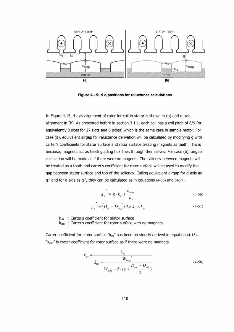
110

Figure 4.15: d-q positions for reluctance calculations

In Figure 4.15, d-axis alignment of rotor for coil in stator is shown in (a) and q-axis

alignment in (b). As presented before in section 3.1.1, each coil has a coil pitch of 8/9 (or

equivalently 3 slots for 27 slots and 8 poles) which is the same case in sample motor. For

case (a), equivalent airgap for reluctance derivation will be calculated by modifying g with

carter’s coefficients for stator surface and rotor surface treating magnets as teeth. This is

because; magnets act as teeth guiding flux lines through themselves. For case (b), airgap

calculation will be made as if there were no magnets. The saliency between magnets will

be treated as a tooth and carter’s coefficient for rotor surface will be used to modify the

gap between stator surface and top of the saliency. Calling equivalent airgap for d-axis as

gd' and for q-axis as gq', they can be calculated as in equations (4-56) and (4-57).

r

mag

cd

hkgg

µ+⋅=

′ (4-56)

( )crcmqsiq kkDDg ××−=

′2/ (4-57)

kc0 : Carter’s coefficient for stator surface kc00 : Carter’s coefficient for rotor surface with no magnets

Carter coefficient for stator surface “kc0” has been previously derived in equation (4-15).

“kc00” is crater coefficient for rotor surface as if there were no magnets.

)2

(5

2

00

00

mbmq

mag

mag

cr

DDgW

Wk

−+⋅+

−

=

λ

λ

(4-58)

111

Having defined equivalent airgap and carter coefficients, equivalent magnetizing

inductance equations for d-axis and q-axis alignments can be derived as in equations

(4-59) and (4-60).

( )′

⋅⋅⋅⋅=

d

pole

wmd

g

AkNL

.4

2

3 02µ

π (4-59)

( )′

⋅⋅⋅⋅=

q

pole

wmq

g

AkNL

.4

2

3 02µ

π (4-60)

Up to now, all sub-components of inductance have been calculated. Total equivalent d-q

axes inductances can be derived by summing all three sub-component values.

mdendslotd LLLL ++= (4-61)

mqendslotq LLLL ++= (4-62)

4.2.3 Calculation of Losses

Beside equivalent circuit parameter calculations, prediction of losses is also a major

requirement, especially if optimization is involved. For PM machines, targets such as high

efficiency and high torque density are in fact contradictory to each other. For example,

high torque density requires reduced machine size with high flux densities. However

higher core losses and lower efficiency arises with high flux densities. To find a good

balance between contradictory requirements, machine loses have to be accurately

predicted also. The main types of losses in PM motors are copper loss, core loss, magnet

loss and mechanical losses due to windage and friction.

Copper Loss

Copper loss of an armature winding can be calculated if resistance of the winding and

armature rms current are known. The resistance of the winding is calculated in Section

4.2.1. The total winding loss is calculated according to

RIPcu ××= 23 (4-63)

where I is the rms value of the armature current and R is per phase resistance. It must be

noted that per phase resistance value has to be modified by equation (4-39) if copper loss

is to be calculated at high or low temperatures different than room temperature.

112

Core Loss

A good estimate of core loss power in steel core of a PM motor can be calculated by FE

numerical computations. However an approximate calculation can be made by equation

(4-64). This analytical equation [45] divides core loss into two components, eddy and

hysteresis loss, and approximates the total loss by loss coefficients.

( ) MBfkBfkP ehloss ×+= 222 ˆˆ Watts (4-64)

In the above equation, kh and ke are hysteresis and eddy loss coefficients respectively, f is

operating electrical frequency, B is peak of flux density and M is total weight of the

medium where loss is calculated.

In the tested motor, core loss variation with frequency has been measured and results are

presented in section 3.2.4. Core loss variation with respect to operating frequency is

measured as in equation (4-65).

ffPloss 0333.00002.0 2 += (4-65)

This expression is related to measured total loss. It is assumed in this study that friction-

windage losses are very small and do not contribute to total loss expression. It is also

assumed that negligible loss appear in the rotor steel since presence of magnets on the

rotor avoids variation of flux densities in time by creating a constant magnetic field. Only

losses appear in stator tooth and back core steel. Equation (4-64) should be solved for

tooth and back-core regions separately as follows.

corebackteethloss PPP −+= (4-66)

The total mass of teeth and back-core area can be calculated by equations (4-67) and

(4-68).

( )

kg

dmkgmmmmmm

mLwhhhNW otsth

15.0

/7.73882.175.1027 3

210

=

××××=

×××++×=

(4-67)

( )

kg

dmkgmmmmmmmm

mLhhDW obcbcsobc

12.0

/7.73825.2)25.262( 3

=

××××−=

⋅⋅⋅⋅−=

π

π

(4-68)

In the equations h0, h1 and h2 are slot dimensions illustrated in Figure 4.11, wt is tooth

width, Dso is stator outer diameter, hbc is stator back core depth behind slot dip, L is axial

length, p is pole number and m0 is weight density of steel core which is 7.7 kg/dm3

113

approximately as given in JFE Steel Catalog No.F1E-001-003 [59]. Reviewing equation

(4-66), equation for total core loss can be derived as in equation (4-69) which includes

losses in teeth and back core of stator.

( ) ( ) bcbcebchththethhcore WBfkBfkWBfkBfkP ⋅++⋅+=222222 ˆˆˆˆ (4-69)

In the above equation Bth and Bbc are tooth and back core peak flux densities calculated as

1.9T and 1.8T respectively. Wth and Wbc are total mass of teeth and back core material. At

this point, all unknowns in equation (4-69) are defined except ke and kh.

The values of kh and ke can be determined by equating the expression in (4-70) to equation

(4-65).

( ) ( )( )( ) ( )( )

fkfk

fkfk

fkfkP

he

eh

ehcore

××+××=

×××+××+

××+××=

93.093.0

12.08.18.1

15.09.19.1

2

222

222

(4-70)

0358.093.0

0333.0==ek (4-71)

000215.093.0

0002.0==hk (4-72)

It is determined that ke can be taken as 0.0358 for and kh as 0.000215 in equation (4-69).

It is assumed here that iron loss of any motor of at 0.33 kW rated power as the sample

motor can be calculated by substituting these kh and ke values into equation (4-69). This

approach is used for the calculation of core loss in the optimization stage.

Core loss resistance can be derived by assigning the calculated core loss into the

equivalent electrical circuit in Figure 4.8. The power loss on a resistor can be calculated by

equation (4-73).

P

VR

R

VP

22

=→= (4-73)

The core loss resistance can be calculated by the same relation in equation (4-73).

( )core

sqq

cP

RIVR

2−

= (4-74)

114

Magnet Losses, Friction and Windage Losses

No detailed analysis has been carried out to determine accurate expressions for magnet,

friction and windage losses. It has been assumed that since magnets have very high

coercivity and resistivity, space harmonics in the armature winding MMF does not induce

eddy currents in the magnets. Friction and windage losses are also neglected regarding to

small dimension of rotor due to low power PM machine (0.33kW rated). However a simple

equation is available, to predict friction and windage losses, which is presented by Gieras [7]. That formula can be used to include these losses in a future study.

4.2.4 Back EMF Voltage

Probably the easiest way of identifying a PM motor is to measure back EMF voltage

waveform because by identifying the generated back-EMF, many property of the tested

motor like EMF and torque constants, pole number, speed range, torque-speed

characteristic can be derived. Also the waveform of the back-EMF tells a lot about the

motor drive requirements like bus voltage and current waveform (sinusoidal or

trapezoidal). So, if the back EMF of a PM motor can be analytically represented, analytical

modelling of the PM motor is completed.

The mathematical expression relating EMF to a square wave shaped magnetic flux

distribution is derived in Chapter 2.3. The derived equation (2-11) must be revised for a

sinusoidal distribution of flux. Also a stacking factor kst and winding factor kw should be

inserted to include effects of laminated stator package and stator winding scheme. The

modified expression is given in equation (4-75).

stwgmo kkNp

E φω2

ˆ = (Vpeak) (4-75)

The flux per pole gφ equals to integration of airgap flux over one pole pitch. Also airgap

mean flux density gB can be multiplied by pole area poleA to calculate gφ . In the equation

(4-75), p is motor pole number, mω is shaft speed in rad/s, N is total number of turns per

phase. In equation (4-75), it is clear that motor EMF voltage is linearly proportional to shaft

speed mω so there can be stated an EMF voltage constant which simplifies the calculation

of EMF voltage at motor terminals at a given shaft speed (equation (4-76)).

stwpolege kkABNp

k2

3= (Vpeak.s/rad) (4-76)

115

4.2.5 Developed Electromagnetic Torque

The torque output of a motor can be calculated by deriving electromagnetic power in the

motor which is simply as in equation (4-77).

IEP oem •⋅= 3 (Watt) (4-77)

In the above equation, per phase EMF rms voltage Eo is multiplied with phase rms current

I to obtain the power output of the motor. This expression is valid under vector control

drive of the motor which states that only q-axis current is excited in motor windings not to

alter flux in the airgap created by magnets.

Also it is known that power at the shaft of a motor can be calculated by multiplying torque

with shaft speed in rad/s. Equation (4-77) can be rewritten to form developed

electromagnetic torque equation.

m

qo

em

IET

ω

⋅=

3 (Watt) (4-78)

The above equation can be written more explicitly by inserting equation (4-75). It must be

noted that the expression in equation (4-75) must be divided by √2 to get rms values

instead of peak.

qstwpolegem IkkABNp

T22

13= (Nm) (4-79)

In the above equation, it is observed that developed torque is linearly proportional to Iq

which states that unless the motor field excitation is changed the motor has a constant

torque constant. The magnetic saturation is ignored in this statement.

stwpolegt kkABNp

k22

13= (Nm /Arms) (4-80)

4.3 Thermal Model

A simplified the thermal model is used in the optimization to reduce complexity of the

optimization and save computation time. The temperature rise per watt loss is calculated

with a thermal constant. The thermal constant “Rth” of the sample motor is measured in

Section 3.3.7 as 2 °K/W. The simplified thermal model to be used in analytical

temperature rise calculations is presented in Figure 4.16.

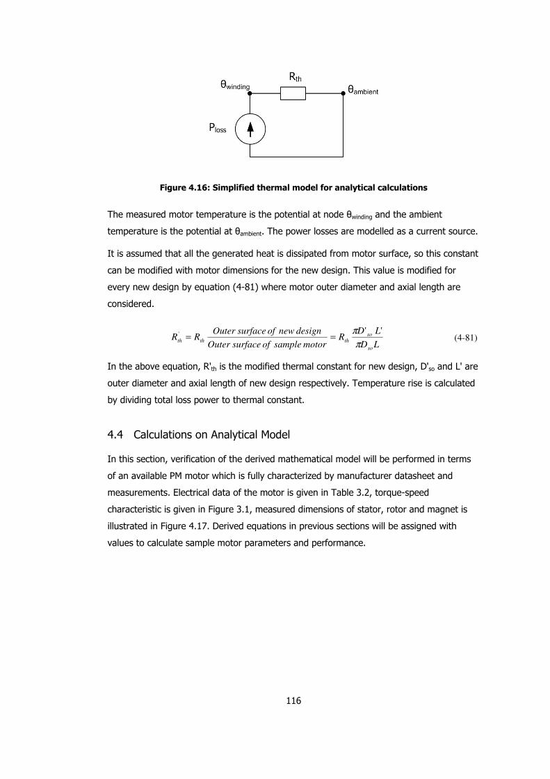
116

Figure 4.16: Simplified thermal model for analytical calculations

The measured motor temperature is the potential at node θwinding and the ambient

temperature is the potential at θambient. The power losses are modelled as a current source.

It is assumed that all the generated heat is dissipated from motor surface, so this constant

can be modified with motor dimensions for the new design. This value is modified for

every new design by equation (4-81) where motor outer diameter and axial length are

considered.

LD

LDR

motorsampleofsurfaceOuter

designnewofsurfaceOuterRR

so

soththth

π

π ''' == (4-81)

In the above equation, R'th is the modified thermal constant for new design, D'so and L' are

outer diameter and axial length of new design respectively. Temperature rise is calculated

by dividing total loss power to thermal constant.

4.4 Calculations on Analytical Model

In this section, verification of the derived mathematical model will be performed in terms

of an available PM motor which is fully characterized by manufacturer datasheet and

measurements. Electrical data of the motor is given in Table 3.2, torque-speed

characteristic is given in Figure 3.1, measured dimensions of stator, rotor and magnet is

illustrated in Figure 4.17. Derived equations in previous sections will be assigned with

values to calculate sample motor parameters and performance.

117

Figure 4.17: Measured dimensions for stator, rotor and magnet of sample motor

4.4.1 Calculation of Flux Densities

Although motor parameter measurements are performed and results are presented in

CHAPTER 3, note that magnet Br value is not indicated yet. The only way to determine Br

is expressing motor EMF or torque constant which include Br expression inside so that Br

can be extracted. Equations with Br expressions are to be calculated after magnet Br value

is calculated from EMF constant derivation.

Magnet cross sectional area by equation (4-3):

2633 103691038107.9 mAmag

−−− ⋅=⋅×⋅= (4-82)

Magnet flux source by equation (4-1):

WbBr

6

0 10369 −⋅×=φ (4-83)

Magnet angle span by equation (4-9):

radmm

mmmag 5875.066.33

5.33

7.9sin2 1 =°=

×= −α

(4-84)

118

Magnet height in each magnet partition by equations (4-6), (4-7) and (4-8):

mmmmmmhmag 2.32.2666.335

2cos5.335.01 =

−

××=

(4-85)

mmDDh mbmagmsmag 53.35

1cos5.02 =

−

×= θ

(4-86)

( ) mmDDh mbmsmag 65.35.03 =−×= (4-87)

Magnet internal reluctance and leakage reluctances by equations (4-5) and (4-11) :

)/(10015.7

1065.3

1

1053.3

2

102.3

2

10385

107.910405.1

1

6

1

3333

37

WbtA

Rmag

−⋅=

⋅+

⋅+

⋅⋅

⋅⋅×

=

−

−−−−

−−π

(4-88)

)/.(1015.7010 6WbtARR magrl ⋅=⋅= (4-89)

Carter’s coefficient for stator surface by equation (4-15):

086.1

1075.0527.1

27.127/1035

27/1035

32

3

3

=

⋅+−⋅⋅

⋅⋅=

−−

−

π

πck

(4-90)

Airgap area by equation (4-16):

26333 1043110381075.025875.0105.332

1mAgap

−−−− ⋅=⋅×

⋅×+×⋅=

(4-91)

Airgap reluctance by equation (4-17):

)/.(105.1

10381075.025875.0105.332

1104

086.11075.0

6

3337

3

WbtA

Rg

⋅=

⋅×

⋅×+×⋅⋅

×⋅=

−−−−

−

π

(4-92)

Stator tooth and back-core reluctances by equations (4-19) and (4-20):

( )WbtARth /.10783/

10381082.110440000

1025.11337

3

=⋅×⋅⋅×

⋅=

−−−

−

π (4-93)

( )( )

WbtARbc /.546010381025.210440000

8/1025.21062337

33

=⋅×⋅⋅×

⋅−⋅⋅=

−−−

−−

π

π (4-94)

Magnet operating flux density by equation (4-24):

119

rrm BBB ⋅=

+

+= 84.0

015.7/5.11

15.70/5.11 (4-95)

Airgap mean flux density by equation (4-26):

rrg BBB ⋅=⋅⋅+

⋅⋅=

−−

705.010015.7/105.11

10431/1036966

66

(4-96)

( )( ) rrg BBB ⋅=⋅×

−

×+×= 59.0705.0

8/75.035

75.025875.02/5.33

π (4-97)

Peak airgap flux density by equation (4-28):

rrg BBB ⋅=×+

= 82.005.175.065.3

65.3ˆ (4-98)

Maximum tooth flux density by equation (4-29):

rrth BBB ⋅=⋅

⋅⋅×=

−

−

83.11082.1

27/103582.0

3

3π (4-99)

Back core flux density by equation (4-31):

r

r

bc BB

B ⋅=⋅×⋅

⋅×⋅⋅=

−−

−

77.110381025.2

10426705.05.033

6

(4-100)

Calculated reluctances and flux densities can be summarized in Table 4.1.

Table 4.1: Calculated reluctances and flux densities for sample motor

Reluctance Calculated Value

(A-t/Wb) Flux Density

Calculated Value (Tesla)

Rmag 7.015 x106 Bg 0.705 x Br (0.74)

Rrl 70.15 x106 gB 0.59 x Br (0.62)

Rg 1.5 x106 Bm 0.84 x Br (0.88)

Rth 1078 Bth 1.83 x Br (1.92)

Rbc 5460 Bbc 1.77 x Br (1.85)

In next section 4.4.2, it is derived from measurements that Br value of tested sample

motor is around 1.05 T. Flux densities in Table 4.1 can be derived by inserting this Br

value into related equations. The calculation results are given in parenthesis in last column

of Table 4.1.

120

4.4.2 Calculation of Electrical Parameters

Phase resistance:

Slot area by equation (4-44):

( )

26

23

333

1027.34

2

1035.4

2

11078.71035.41055.2

2

1

m

Aslot

−

−−−−

⋅=

⋅+⋅⋅⋅+⋅= π

(4-101)

Wire cross section area by equation (4-34):

266

1045.14

339.01027.345.0mAwire

−−

⋅=⋅⋅⋅

= (4-102)

Conductor length in one coil by equation (4-35):

( ) mLwire 55.0011.0035.027

3015.0038.042 =

⋅+++⋅×= π (4-103)

Length conductor for connecting coils in series by equation (4-36):

( ) mLcon 43.0015.092011.0062.027

39=××+−

×= π (4-104)

Total phase resistance by equation (4-38):

( )Ω=

⋅

+×⋅=

−

− 062.01045.1

43.055.091068.1

6

8R (4-105)

d-q axes Inductances:

Slot leakage permeance coefficients by equations (4-45), (4-46) and (4-47):

6

00 10135.4

235.4

3

1

27.1

8.0623.0

2

1 −⋅=+

+= µµpT (4-106)

6

0 1083.235.455.2

2

35.4275.8

227.1

8.0 −⋅=

+

−+= µpB (4-107)

6

0 1081.135.455.2

2

35.478.7

27.1

8.0 −⋅=

+

−+= µpTB (4-108)

121

Slot leakage inductance by equations (4-40), (4-41) and (4-42):

( )( )

mH

Lsls

032.0

286.031081.121083.21027

038.0363 6662

=

−×⋅⋅⋅+⋅+××

= −−−

(4-109)

( ) HLslm

662

1016.486.0131081.127

038.0363 −− ⋅=−⋅×⋅××

= (4-110)

mHLslot 037.01016.41045.32 66 =⋅+⋅= −− (4-111)

End-winding inductance by equations (4-48), (4-50), (4-51) and (4-49):

( ) mwc 017.027

3011.01025.2062.0 6

1 =−⋅−= −π (4-112)

mL e 047.0017.0015.021 =+⋅= (4-113)

3.0047.0

017.021

83

2734.0 =

−⋅

⋅⋅=

πλend

(4-114)

mHLend 011.03.0047.08

364

2

0 =×= µ (4-115)

Magnetizing inductance calculation by equations (4-56) (4-60):

56.1

2/)3035(57.9

7.978.11

78.112

=

−⋅+−

=crk

(4-116)

mg d

33 1029.405.1

65.3086.11075.0 −− ⋅=+×⋅=

′ (4-117)

( ) mgq

333 1023.456.1086.12/10301035 −−− ⋅=××⋅−⋅=′

(4-118)

( ) mHLmd 041.01029.4

10511.94.036

8

14

2

33

6

02=

⋅

⋅⋅×⋅⋅⋅=

−

−µ

π (4-119)

( ) mHLmq 042.01023.4

10511.94.036

8

14

2

33

6

02=

⋅

⋅⋅×⋅⋅⋅=

−

−µ

π (4-120)

Total inductance by equations (4-61) and (4-62):

mHLd 089.0041.0011.0037.0 =++= (4-121)

mHLq 090.0042.0011.0037.0 =++= (4-122)

122

EMF and Torque Constants:

EMF and Torque constants by equations (4-76) and (4-80):

( ) rre BBk ×=××⋅×⋅××= − 067.095.094.01051159.0362

83 6 (Vpeak.s/rad) (4-123)

( ) rrt BBk ×=××⋅×⋅×= − 082.095.094.01051159.0362

8

2

13 6 (Nm /Arms) (4-124)

In manufacturer’s datasheet, it is stated that ke is 0.071 Vpeak.s/rad and kt is 0.086

Nm/Arms. Inserting these given values to equations (4-123) and (4-124) magnet Br is

calculated as 1.05 T by equations (4-125) and (4-126).

TBB rr 05.1067.0071.0 =→×= (4-125)

TBB rr 05.1082.0086.0 =→×= (4-126)

It can be concluded that the magnets in the sample motor have Br value of at least 1.05T.

NdFeB magnets are classified with respect to operating temperature and Br values by

manufacturers. The sample motor has H class insulation which is to be operated up to

150°C. At this operating temperature, NdFeB magnets have a Br value of around 1.05T

are 28SH, 30SH, 28UH, 30UH [57]. The most probable candidate is 30UH with temperature

rating 180°C and minimum Br value of 1.08T (see Table 4.2) because the presented

values by the manufacturer is theoretical values for simple shaped magnets which do not

include coating. Final product from the manufacturer will have slightly lower Br value due

to coating and shaping of the magnets.

A slightly higher Br value for the magnet should be selected for prototyping because

demagnetization may occur in manufacturing the motor.

Table 4.2: Magnetic Characteristics and Physical Properties of Sintered NdFeB [57]

Magnet

Grade

Remanence

Br (T)

Coercive

Force Hcb

(kA/m)

Intrinsic

Coercive Force

Hcj (kA/m)

Max Energy

Product BHmax

(kJ/m3)

Max Working

Temperature (°C)

30UH 1.08-1.13 ≥ 812 ≥ 1990 223 - 247 ≤180

123

4.4.3 Calculation of Torque-Speed Characteristic

Having defined all equivalent circuit parameters, performance characteristics of the PM

machine such as torque-speed and power-speed can be analytically determined. To do

this, equivalent electrical circuit should be solved at some speed steps to determine

current and then torque and power output can be calculated easily by multiplying torque

constant kt with the current value.

In this thesis work, for each 100rpm speed step starting from 1rpm and up to 5001rpm,

equivalent electrical circuit is solved and motor terminal current is determined. The related

equations and assumptions are presented in Chapter 2.2. Bus voltage is 21VDC and

maximum current limit is 35Arms as in sample motor manufacturer datasheet.

Figure 4.18: Measured and analytically calculated Torque-Speed characteristic of sample

PM motor

In Figure 4.18, measured torque values are marked with “∆” whereas analytically

calculated maximum torque curve is plotted with dashed line. As observed in the figure,

analytical and measurement values agree well with each other.

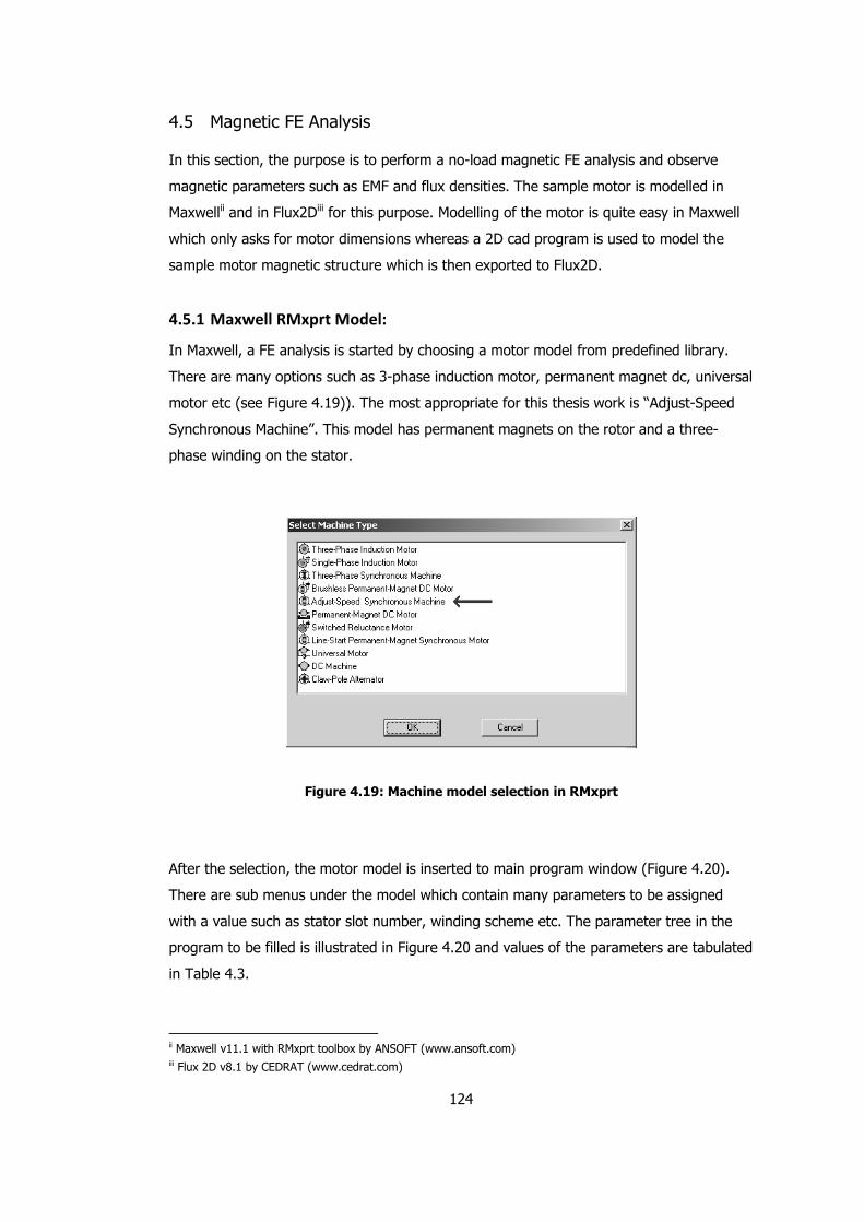
124

4.5 Magnetic FE Analysis

In this section, the purpose is to perform a no-load magnetic FE analysis and observe

magnetic parameters such as EMF and flux densities. The sample motor is modelled in

Maxwellii and in Flux2Diii for this purpose. Modelling of the motor is quite easy in Maxwell

which only asks for motor dimensions whereas a 2D cad program is used to model the

sample motor magnetic structure which is then exported to Flux2D.

4.5.1 Maxwell RMxprt Model:

In Maxwell, a FE analysis is started by choosing a motor model from predefined library.

There are many options such as 3-phase induction motor, permanent magnet dc, universal

motor etc (see Figure 4.19)). The most appropriate for this thesis work is “Adjust-Speed

Synchronous Machine”. This model has permanent magnets on the rotor and a three-

phase winding on the stator.

Figure 4.19: Machine model selection in RMxprt

After the selection, the motor model is inserted to main program window (Figure 4.20).

There are sub menus under the model which contain many parameters to be assigned

with a value such as stator slot number, winding scheme etc. The parameter tree in the

program to be filled is illustrated in Figure 4.20 and values of the parameters are tabulated

in Table 4.3.

ii Maxwell v11.1 with RMxprt toolbox by ANSOFT (www.ansoft.com) iii Flux 2D v8.1 by CEDRAT (www.cedrat.com)

125

Figure 4.20: Model details to be filled in RMxprt

Table 4.3: Maxwell RMxprt parameter values to model sample PM machine

Menu Parameters Values

Machine Number of Poles Rotor Position Frictional Loss Wind Loss Reference Speed Control Type Circuit Type

8 Inner rotor 0 0 2200rpm PWM Y3

Circuit Transistor Drop Diode Drop Modulation Index Carrier Frequency

0 0 0.99 60

Stator Outer Diameter Inner Diameter Length Stacking Factor Steel Type Number of Slots Slot Type Skew Width

62 35 38 0.95 steel_RM23 27 1 0

126

Table 4.3: Maxwell RMxprt parameter values to model sample PM machine, contd.

Slot Auto Design Parallel Tooth Tooth width Hs0 Hs2 Bs0

False True 1.82 0.8 7.78 1.27

Winding Winding Layers Winding Type Parallel Branches Conductors per Slot Coil Pitch Number of Strands Wire Wrap Wire Size

2 Whole Coiled 1 8 3 1 0 0

End/Insulation Input Half-turn Length End Adjustment Base Inner Radius Tip Inner Diameter End Clearance Slot Liner Wedge Thickness Layer Insulation Limited Fill Factor

False 15 1 1 0.25 0.5 0.25 0.25 0.4

Rotor Outer Diameter Inner Diameter Length Steel Type Stacking Factor Pole Type

33.5 11 38 steel_RM23 0.95 3

Pole (Magnet Properties)

Embrace Offset Magnet Type Magnet Thickness

0.748 0 NdFe30 3.65

Shaft Magnetic Shaft False

BH Curve of the electrical steel (defined as steel_RM23 in Table 4.3) is presented in Figure

4.21. It can be observed that the electrical steel begins to saturate at around 1.8T and

fully saturates at 2.1T.

127

0

0,5

1

1,5

2

2,5

0 20000 40000 60000 80000 100000

H (A/m)

B (

T)

Figure 4.21: B-H curve for electrical steel

In Figure 4.22, induced EMF voltage waveforms in motor windings calculated by Maxwell

are presented. It can be observed in the figure that at 1000rpm, peak of EMF voltage at

motor terminals is 7.20V which states that EMF constant ke is 0.069Vpeak.s/rad. If one

inserts the presented parameter values in Table 4.3 into RMxprt, same results as

presented in Table 4.4 can be expected.

Figure 4.22: Induced voltage waveforms at 1000rpm for sample motor in Maxwell

128

4.5.2 Flux2D Model:

The magnetic structure of the sample motor is created in a CAD program with respect to

mechanical dimensions presented in Figure 4.17. The created 2D model is then exported

to Flux2D program. Proper meshing is applied to the model as presented in Appendix.

Magnets are assigned from program library as NdFe30. A sample view of the Flux2D model

is illustrated in Figure 4.23.

Figure 4.23: 2D cad model used in Flux2D for FE analysis

Note: Arrows in the figure show magnetization direction of magnets

Figure 4.24: Motor equivalent circuit model in Flux2D for FE analysis

129

Transient magnetic solution is performed to determine EMF at motor terminals. Motor

electrical equivalent circuit is modelled as in Figure 4.24. In the circuit “R4, R5, R6, R7” are

inserted to sense voltage across terminals and phase. Their resistance is infinite with

respect to phase resistances so that it can be assumed no current passes through. Motor

terminals are presented in the figure as “A, B, C”. The end winding resistance is assigned

so that total phase resistance is 0.068 ohm. Flux2D calculated phase resistances as 0.032

ohm, so end winding resistance is assigned as 0.036ohm. The value of end winding

inductance is assigned as calculated with equation (4-115) in Chapter 0.

The transient FE analysis is performed with such time steps that in one electrical period

there are 50 data points. A sample waveform of back EMF voltage for sample motor at

750rpm is presented in Figure 4.25. Peak value of fundamental harmonic of presented

EMF voltage waveform at motor terminals is 5.39V which states that EMF constant ke is

0.069 Vpeak.s/rad.

Figure 4.25: Induced voltage waveforms at 750rpm for sample motor in Flux2D

Summary of the results of FE analysis from both Maxwell and Flux2D programs are

tabulated in Table 4.4.

4.6 Comparison of Analytical Results with Measurements and FE Analysis

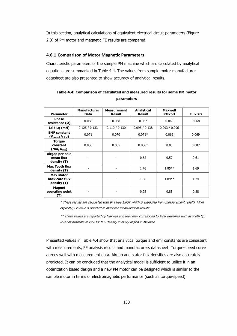
130

In this section, analytical calculations of equivalent electrical circuit parameters (Figure

2.3) of PM motor and magnetic FE results are compared.

4.6.1 Comparison of Motor Magnetic Parameters

Characteristic parameters of the sample PM machine which are calculated by analytical

equations are summarized in Table 4.4. The values from sample motor manufacturer

datasheet are also presented to show accuracy of analytical results.

Table 4.4: Comparison of calculated and measured results for some PM motor

parameters

Parameter Manufacturer

Data Measurement

Result Analytical Result

Maxwell RMxprt Flux 2D

Phase resistance (Ω)

0.068 0.068 0.067 0.069 0.068

Ld / Lq (mH) 0.125 / 0.133 0.110 / 0.130 0.095 / 0.138 0.093 / 0.096 -

EMF constant (Vpeak.s/rad)

0.071 0.070 0.071* 0.069 0.069

Torque constant (Nm/Arms)

0.086 0.085 0.086* 0.83 0.087

Airgap per pole mean flux density (T)

- - 0.62 0.57 0.61

Max Tooth flux density (T)

- - 1.76 1.85** 1.69

Max stator back core flux density (T)

- - 1.56 1.89** 1.74

Magnet operating point

(T) - - 0.92 0.85 0.88

* These results are calculated with Br value 1.05T which is extracted from measurement results. More

explicitly; Br value is selected to meet the measurement results.

** These values are reported by Maxwell and they may correspond to local extremes such as tooth tip.

It is not available to look for flux density in every region in Maxwell.

Presented values in Table 4.4 show that analytical torque and emf constants are consistent

with measurements, FE analysis results and manufacturers datasheet. Torque-speed curve

agrees well with measurement data. Airgap and stator flux densities are also accurately

predicted. It can be concluded that the analytical model is sufficient to utilize it in an

optimization based design and a new PM motor can be designed which is similar to the

sample motor in terms of electromagnetic performance (such as torque-speed).

131

4.6.2 Analytical Determination of Torque-Speed Characteristic

In previous sections, an electrical equivalent PM motor model is formed and parameters in

the model are measured. The model can be verified by inserting parameter values in the

equivalent circuit and solving it to determine terminal current.

In laboratory, the tested PM machine is driven by vector control where only q-axis current

is present in the motor windings.

Figure 4.26: Sample motor q-axis electrical equivalent with parameter values

Since it is assumed that there is no d-axis current, the parameter “w.Ld.Id” is assigned with

zero volt in the above figure.

Table 4.5: Calculated torque values with equivalent PM motor model

Shaft Speed (rpm)

Measured Terminal Voltage (Vrms line)

Calculated EMF

Voltage (Vrms line)

Calculated Core Loss Resistance (ohm)

Calculated Xq (ohm)

Calculated Line

Current (Arms)

Calculated Torque (Nm)

500 5,99 2,59 5,23 0,027 35 2,94

1000 9,54 5,18 9,34 0,054 35 2,94

1500 13,08 7,78 12,35 0,082 35 2,93

1700 14,50 8,81 13,24 0,093 35 2,92

1800 14,85 9,33 13,62 0,098 32,8 2,74

2000 14,85 10,37 14,24 0,109 25,1 2,07

2200 14,85 11,40 14,69 0,120 18,2 1,48

2500 14,85 12,96 15,03 0,136 9,2 0,71

2800 14,85 14,51 14,96 0,152 1,5 0,04

132

Figure 4.27: Comparison of sample PM motor torque-speed characteristics from

manufacturer datasheet, measurements and calculations

It is observed in Figure 4.27 that all three torque-speed characteristics agree by 1% ‘n

constant torque region whereas a 5% disparity occurs in constant power region. The

consistency of calculated characteristic with measured and datasheet shows that the

equivalent motor model is correct and measured parameter values are sufficiently

accurate.

133

CHAPTER 5

OPTIMUM DESIGN of a PM MOTOR

In this chapter, a mathematical design optimization strategy will be developed with the

analytical model presented in CHAPTER 4. The aim of optimized design is to find an

optimum balance between expected performance requirements and volume of the

designed machine.

A multi-objective optimization problem consists of objectives associated with inequality and

equality constraints. The optimisation problem as a constrained minimization problem can

be defined in n-dimensional calculation space where n is equal to the number of optimized

parameters. Mathematically, the problem can be expressed as follows:

Minimize / Maximize fi ( X ) i = 1, 2, …. N

Subject to; gj ( X ) ≤0 j = 1, 2, …J

hk ( X ) = 0 k = 1, 2, ….K

It is stated with this expression that an optimization problem consists of an objective

function fi () and constraint functions gj (), hk ( X ) which are a function of design

vector X . The X is a p dimensional vector with n design or decision variables (equivalently

n dimensions). The design vector X consists of independent design variables which are to

be varied to find the optimum design vector mX . Therefore there is a need for a model

from which the performance of the motor can be calculated. The parameters of the model

need to be calculated in terms of design vector members which are generally selected

from motor dimensions.

In this thesis work, the analytical model developed in CHAPTER 4 is preferred. As shown in

Section 4.6, this model is capable of predicting the motor performance with good

accuracy. Employing FE analysis for motor optimum design is not a practical proposition.

During optimum design, repetitive performance calculations are required. Due to

numerous parameters affecting motor performance, the solution time becomes

unacceptably long. FE analysis can be used later to assess the optimal solution.

134

5.1 Definition of the Optimization Problem

5.1.1 Specifications

The designed motor is expected to satisfy some performance requirements within defined

system boundaries. Calculated performance parameters are output torque, input power,

efficiency in entire current and speed range. Parameters in equivalent electrical and

magnetic circuit of the motor are calculated for each new design and inserted into

performance calculations. These are per phase resistance, d-q axis inductances, core loss

current, back EMF voltage, flux densities (airgap, tooth, back core).

The designed motor shall be capable of delivering minimum of 330 W at 2000 rpm.

Reference calculations (such as torque and power output, efficiency, temperature rise) are

going to be performed at 2000 rpm. Motor shall be capable of delivering up required

performance up to 150°C temperature for stator winding.

The motor is going to be driven by vector controlled 3 phase inverter assuming that the

bus voltage is necessary to supply 21 Vpeak line-line voltage at motor terminals. The motor

is driven with vector control method and no field weakening is to be applied during

operation. The phase diagram of this drive method is presented in Figure 3.19-a. The

inverter has 3-phase sinusoidal current outputs with a maximum current of 35Arms.

The motor must have 8 poles as required by the motor drive system. The back EMF

voltage is also expected to have a sinusoidal waveform. For this reason, different slot

number combinations (such as 9, 15, 18, 21, 24, 27, 30, 36) are inspected where

maximum EMF voltage with minimum harmonic distortion is aimed. As presented in the

book by Hanselman [8], the most suitable slot number for 8 poles is 27 in terms of

minimum harmonic winding coefficients. For this reason, the motor slot/pole ratio is fixed

as 27/8 for the design.

It must be noted that 27 slot – 8 pole combination results slot/pole/phase number as

1.125 which is fractional. This number is an integer every 8 coils which states that winding

scheme repeats it self every 8 poles. Since there can be only 9 coils in 27 slots for three

phase, all coils have to be connected in serial inevitably. If the slot number is selected as

30, slot/pole/phase number is 1.25 and winding can be constructed of 8 coils where 4 coils

are in parallel with other 4 coil group.

135

The outer diameter of the motor can be 65 mm at maximum due to packaging issues. The

housing has a hollow body with 65 mm inner diameter. Also rotor is going to be mounted

on 11 mm shaft which limits rotor inner diameter.

The airgap of the motor is first selected as 0.5mm assuming that this space is sufficient to

allow free run of rotor with a bandage over magnets. In first prototypes heat-shrink tubes

were used and it is observed that the width of the tubes after heating may vary much. It is

decided that 0.5mm is not sufficient for safe operation so that the minimum airgap was

presumed to be larger than 0.75mm and it should be defined in the optimization in this

way. On the other hand, theoretically, it is evident that the optimum airgap is the

minimum allowable so it is wise to fix the airgap width rather than search for optimum

value. For this reason, the airgap width is fixed as 0.75mm in the optimization after

considering manufacturing issues.

No mechanical requirements are defined such as mass and inertia. The optimization aims

to reach the minimum volume within the defined criteria, so it is also assumed that the

optimum design has the minimum feasible mass and inertia.

Steady state torque - speed curve of the motor is calculated by the analytical equations in

CHAPTER 4. In these calculations there are many motor parameters such as dimensions

and electrical parameters. Some of them are chosen to be a member of design vector.

Others can be expressed in terms of selected design vector variables and some constant

parameter values. The design vector elements are defined in Section 5.1.4 as independent

variables.

The proposed simple thermal model in Section 4.3 will be used to predict the thermal

behaviour of the new design. Calculated power loss will be inserted into the thermal model

to determine temperature rise under specific loading condition.

136

Table 5.1: Specifications table for the new motor design

Specification Sample

Motor Value Design

Specification Remark

Number of poles 8 8 Pre-defined to be compatible with available motor driver

Slot number 27 27 Selected by harmonic investigation from the book by Hanselman [8]

Motor Terminal voltage

21 Vpeak line-line

21 Vpeak line-line Maximum value of motor terminal voltage. Assuming DC bus voltage is enough to allow drive to generate this voltage.

Airgap 0.75 mm 0.75 mm Pre-defined for all designs

Outer Diameter 62 mm 65 mm Maximum feasible value

Peak torque 3 Nm 3 Nm Minimum peak torque at 1500 rpm. This also defines peak stall torque to be at least 3Nm.

Rated power 330 W 330 W Minimum delivered mechanical power at 2000 rpm

Max Speed 2820 rpm - No maximum speed specification is defined.

Winding connection Serial Serial All coils in each phase are connected in series

EMF constant 0.071 Vpeak.s/Rad

- No EMF constant specification is defined.

Torque constant 0.086 Nm/Arms - No torque constant specification is defined.

Temperature rise at rated speed and load

100°C 100°C Motor is hanging in the air.

Resistance 0.067 Ω - Per phase resistance

Inductance 0.237 mH - Terminal to terminal inductance

Mass 2.3 kg No specification for mass is defined.

Inertia 0.6 kg.cm2 No specification for inertia is defined.

5.1.2 Objective Function

The aim of this study is to have most efficient electromagnetic energy conversion in the

smallest volume. For this purpose, two main parameters of the optimized motor design

are:

1. Maximize efficiency

2. Minimize volume

On the other hand, to minimize torque rippler, a constraint is placed on the airgap flux

density harmonics as discussed in Section 5.1.3.

These two objectives are in fact contradictory to each other since high efficiency comes

with larger volume which has more space for copper, lower flux density in the core, larger

flux linkage per pole. The two objective functions are weighted to define a single cost

function because two functions have incomparable values. Effect of efficiency variation will

dominate variation in volume. For this purpose, sample motor efficiency at selected

reference speed (2000 rpm) and volume are used to normalize two objectives and define a

single cost function as in equation (5-2).

137

effvolt fkfkf max2min1cos += (5-1)

The defined weights k1 and k2 sum up to 1 which states k2 = 1-k1. Optimization can be

performed in terms of trade off between efficiency and minimized volume by adjusting the

weights of k1 and k2. By defining a single cost function, the optimization is no longer a

multi-objective, but a scalar objective optimization.

Normalized values for efficiency and volume will be very useful in terms of deciding

whether the new design is better than the sample motor according to defined weights.

Normalization of the calculated volume and efficiency for new design can be done by

dividing each term to sample motor values as in equation (5-2).

designnew

motorsample

motorsample

designnew

tEff

Effk

V

Vkf 21cos += (5-2)

Considering the sample motor volume and efficiency at selected operating point (2000rpm,

21 Vpeak line-line voltage), equation (5-2) can be explicitly written as in equation (5-3).

designnew

designnew

tEff

Vf

73.050.0

108.11450.0

6cos +×

=−

(5-3)

The defined cost function outputs “1” for same volume and efficiency as sample motor. A

new design with objective function value smaller than 1 means a better design than

sample motor with the defined cost function. This cost function is to be minimized with the

optimization.

5.1.3 Constraints

A constraint can be defined as a boundary which must be satisfied by the optimized

system. Constraints may be due to various reasons such as;

Performance constraints: Max torque, Max speed, No load current etc…

Manufacturing difficulties or realization limits: Minimum airgap, Minimum tooth

width, Outer diameter etc…

Material properties: Saturation level of electrical steel etc…

The outer diameter is selected to be 65mm at maximum because the designed stator is

going to be fit into an available motor housing and the maximum allowable inner diameter

is 65 mm due to workmanship.

138

Maximum flux densities in teeth and back core are limited as 1.89T and 1.77T respectively

which are the calculated densities in the sample motor.

Motor peak stall torque is defined as a specification by the manufacturer of the sample

motor. However in this study, instead of defining a stall torque, peak torque at 1500rpm is

defined as a specification. PM machines torque characteristic consists of two regions;

constant torque region and constant power region where torque is monotonically

decreasing (see Figure 3.1). So, if output torque at a speed is defined than it can be

concluded that stall torque is at least that value due to monotonically decreasing torque

characteristic. In this work, by defining output torque of 3Nm at 1500rpm, stall torque is

defined indirectly which states that peak stall torque is also at least 3Nm.

Rated torque and speed are also given as a performance specification by the

manufacturer. In this work, no torque or EMF constant is defined as a specification, but

instead torque output at 1500rpm and 2000rpm are defined as electromagnetic output

performance specification which defines EMF and torque constants indirectly as well.

Constraints for slot width, back core depth, tooth width and magnet displacements are all

to ensure feasibility of realization of the design. For example, a design with 0.1mm tooth

width is not realizable with the machinery available to be used for this thesis work.

The available motor drive is capable of supplying 35-40Arms peak and 15-20Arms to a

motor. For this reason, the rated current of the designed motor is defined to be lower or

equal to 20Arms to be compatible with the drive. The current density is also defined to be

lower or equal to 12Arms which is the calculated value for the sample motor.

In the specifications, it is stated that the designed motor is expected to develop minimum

3Nm at 1500rpm, deliver 330W at 2000rpm and the temperature rise must be maximum

of 100°C at 2000rpm which defines the rated speed of the motor. All these three

specifications are introduced as constraints in the optimization.

The defined design constraints for the optimization are tabulated in Table 5.2. The BH

curve for the electrical steel to be used for lamination is presented in Figure 5.1.

139

Table 5.2: Design constraints for optimization

Constraint Vector element

Constraint name Limit Remark

g1 Stator outer diameter “Dso” ≤ 65mm Motor housing does not allow larger outer diameter

g2 Peak Tooth flux density “Bth” ≤ 1.89T Calculated flux density in sample motor

g3 Peak Stator yoke flux density “Bbc” ≤ 1.77T Calculated flux density in sample motor

g4 Slot width at lower side “w1” ≥ 1mm This ensures that final design does not have a closed slot bottom

g5 Back-core depth “hbc” ≥ 1mm Minimum width from manufacturing limitations

g7 Tooth width “Wth” ≥ 1mm Thinner tooth width may be unrealizable

g8 Displacement between two magnet tips (rotortest)

≥ 1mm This ensures that two successive magnets on the rotor do not interfere with each other (Figure 5.2).

g6 THD of airgap flux density due to magnets

≤ 8% A sinusoidal flux distribution is aimed

g9 Rated current “Irated” ≤ 20Arms This ensures that final design is compatible with available motor drive.

g10 Rated current density “Jrated” ≤ 12Arms/mm2 This value is selected based on a thermal model.

g11 Maximum torque output at

1500 rpm “maxTeref” ≥ 3 Nm

The operating range of the system is aimed to be 0-1500rpm where 3Nm peak torque is demanded

g12 Rated power output at reference speed (2000rpm) “Pref”

≥ 330 W The designed motor should be capable of delivering 330W at 2000rpm.

g13 Temperature rise at reference speed (2000rpm) “Tempref”

≤ 100 °C Temperature rise at reference speed at reference power must not exceed 100°C

0

0,5

1

1,5

2

2,5

0 20000 40000 60000 80000 100000

H (A/m)

B (

T)

Figure 5.1: B-H curve for electrical steel used in design

140

There are geometrical constraints also such as minimum tooth width and displacement

between two magnet tips to ensure mechanical realization (rotortest variable in Figure

5.2). Too small dimensions may not be realizable in manufacturing. In this thesis work,

minimum mechanical dimension is chosen to be 1mm such that there is no part in

lamination (i.e. tooth width, tooth tip, back core) that is thinner than 1mm.

Torque ripple is not calculated analytically in the developed analytical model. However the

amplitude of ripple is a very important criterion for PM machines and minimum torque

ripple is always preferred for highest performance. To consider this issue, harmonic

distortion of airgap flux distribution is included in the constraints. Theoretically, in PM

machines, the torque is developed by interaction of airgap flux with current in stator

windings. So, if there is no harmonic in airgap flux or stator, no harmonic torque resulting

ripple can be developed. For this reason, THD of airgap flux distribution is included in the

constraints to have the minimum torque ripple in the design. It must be noted that

cogging torque is different than torque ripple which results from interaction of rotor

magnets with stator inner surface structure.

Figure 5.2: Rotortest constraint to check rotor structure feasibility

The defined constraints are defined in modeFrontier as “less than” (<) or “greater than”

(>) since there is no option to define as “equal or less/greater than” (≤, ≥). Also all

parameter magnitudes are represented by 20 digit numbers in the program. For example

an outer diameter magnitude of “62mm” is defined as “0.062000000000000000”. The

handicap of this magnitude representation is that even unfeasible variations in real life

such as 1 nm are taken into consideration which decreases the efficiency of the

optimization.

The effect of magtnitude representation to optimization convergence is studied in Section

5.5 by running the optimization with variation steps defined for each design variable.

141

5.1.4 Independent Variables

The independent design variables are the machine parameters which constitute design

vector X and vary during optimized design process. Independent variables have to be

selected so that all other dimensions can be expressed of these variables. For example, if

stator inner diameter Dsi and rotor outer diameter (diameter at magnet surface) Dms are

design variables, then airgap g should be discarded as a variable because it has already

been defined by these two diameters.

( )mssi DDg −=2

1 (5-4)

The selected independent design variables with their limits for this thesis work are listed in

Table 5.3. As observed, some of them discrete variables because it has no sense to define

continuous variable space. The axial length is dependent on steel lamination which has

0.5mm thickness, so the length in axial direction can be in 0.5 steps. Also winding coil

turns is in discrete steps of one ranging from 1 to 6. This limit is set to avoid unnecessary

search of coil turns in wide range. Slot depth defines the slot area where the upper limit is

set based on geometrical observations based on the defined 65 mm outer diameter limit.

Minimum tooth width is set as 1 mm as narrower geometry may not be realizable and the

upper limit is set also with respect to geometrical observations based on 65 mm outer

diameter. The same situation is valid also for stator yoke (back-core) height.

Magnet Br value range is defined with respect to product list magnets from a magnet

manufacturer [Appendix A.5]. On the other hand, magnet height is set free on the

continuous range (1…5 mm) by interpretation of geometrical limitations.

Table 5.3: Independent variables in optimized design of a PM machine

Independent variable Vector element

Independent

Variable Name

Abbreviation

(Figure 5.3)

Variable

Type Limits

x1 Axial length L discrete by 0.5mm

steps 30mm < L < 50mm

x2 Slot depth h1 continuous 5mm < h1 < 12mm

x3 Stator yoke height hbc continuous 1mm < hbc < 4.5mm

x4 Tooth width Wth continuous 1mm wth < 3.5mm

x5 Diameter at magnet base Dmb continuous 20mm < Dmb < 40mm

x6 Magnet height hmag continuous 1mm < hmag < 5mm

x7 Magnet arc span in one pole pitch

alfa continuous 0.6 ≤ alfa ≤ 0.9

x8 Turns per coil Nturn discrete by 1 steps 1 ≤ Nturn ≤ 6

142

x9 Magnet Br Br discrete by 0.02T

steps 1.15 ≤ Br ≤ 1.25

The defined variable “alfa” which relates magnet pitch to one pole pitch is illustrated in

Figure 5.4. Multiplication of “alfa” with one pole pitch gives magnet pitch.

Figure 5.3: Corresponding dimensions for geometric abbreviations of design variables

143

Figure 5.4: Figure showing one pole pitch and magnet pitch

5.1.5 Dependent Variables

Dependent variables are defined as motor dimensions which can be calculated with

evaluation of independent variables together with constant parameters. The dependent

variables are listed in Table 5.4.

Table 5.4: Dependent variables in optimized design of a PM machine

Dependent Variable Abbreviation

(Figure 5.3) Value

Diameter at magnet surface Dms Dmb + 2.hmag

Diameter at stator inner surface Dsi Dms + 2.g

Slot width at narrow side w1 ( )( ) th

slot

si wN

mmhD −++π

5.02 0

Slot width at wider side w2 ( )( ) th

slot

si wN

hmmhD −+++π

15.02 0

Slot bottom radius h2 w2 / 2

Diameter at stator outer surface

Dso ( )20 15.02 hhmmhDsi ++++

Magnet width wmag

⋅

palfaDms

360

2

1sin

In Table 5.4, calculations of dependent variables are also illustrated in the last column.

The 0.5mm clearance defined in w1, w2 and Dso expressions is corresponding to slot liner

thickness which is used to close the slot opening to avoid windings to slip out (see Figure

5.5).

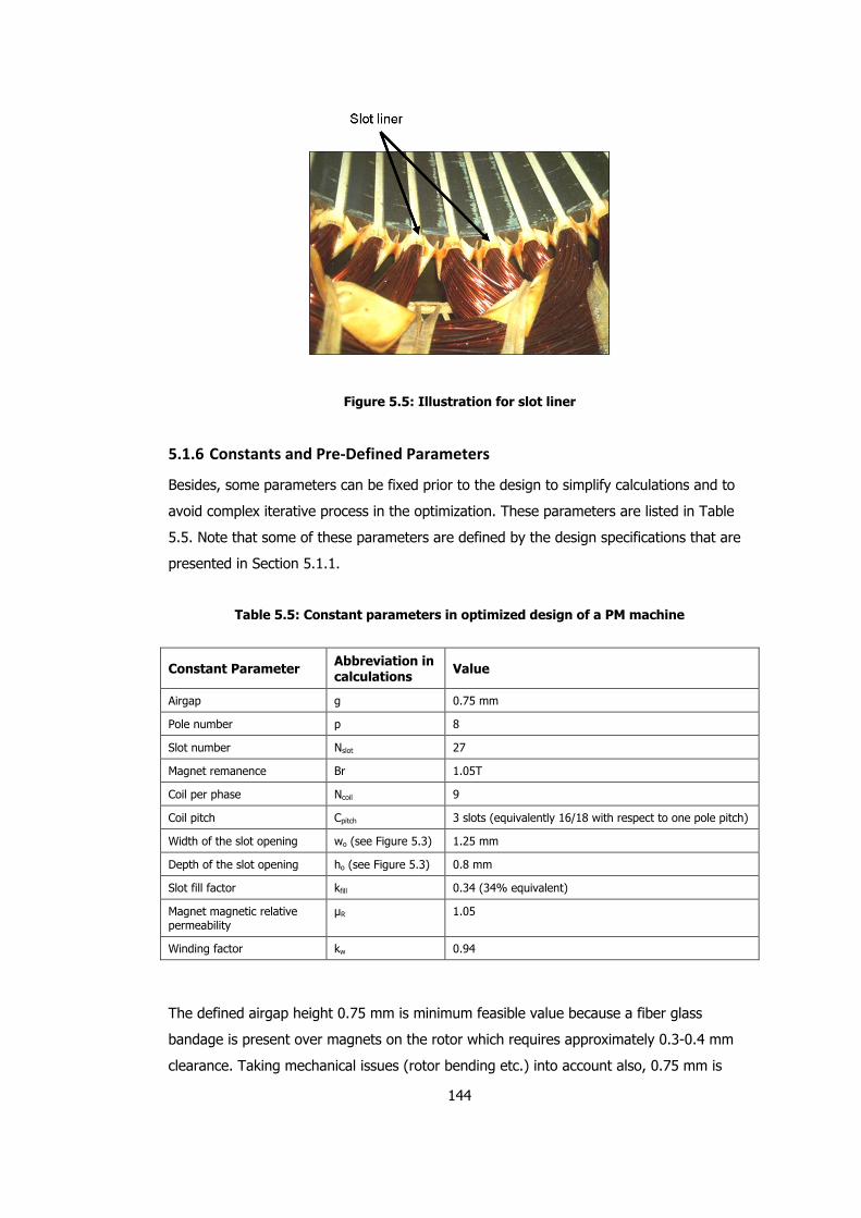
144

Figure 5.5: Illustration for slot liner

5.1.6 Constants and Pre-Defined Parameters

Besides, some parameters can be fixed prior to the design to simplify calculations and to

avoid complex iterative process in the optimization. These parameters are listed in Table

5.5. Note that some of these parameters are defined by the design specifications that are

presented in Section 5.1.1.

Table 5.5: Constant parameters in optimized design of a PM machine

Constant Parameter Abbreviation in calculations

Value

Airgap g 0.75 mm

Pole number p 8

Slot number Nslot 27

Magnet remanence Br 1.05T

Coil per phase Ncoil 9

Coil pitch Cpitch 3 slots (equivalently 16/18 with respect to one pole pitch)

Width of the slot opening wo (see Figure 5.3) 1.25 mm

Depth of the slot opening ho (see Figure 5.3) 0.8 mm

Slot fill factor kfill 0.34 (34% equivalent)

Magnet magnetic relative permeability

µR 1.05

Winding factor kw 0.94

The defined airgap height 0.75 mm is minimum feasible value because a fiber glass

bandage is present over magnets on the rotor which requires approximately 0.3-0.4 mm

clearance. Taking mechanical issues (rotor bending etc.) into account also, 0.75 mm is

145

chosen as airgap height. Since the designed motor is to be integrated to the available

driver on a system, the pole number is restricted as 8. Number of slots

5.1.7 Performance Calculations

During the design process, the performance (torque, power, current etc.) of the motor is

going to be calculated for each new design vector X according to the model presented in

CHAPTER 2. The equivalent circuit of the motor for performance calculations under vector

control is given in Figure 2.3. It must be noted that since it is assumed that the motor is

driven by vector control, no d-axis excitation is present and only the q-axis equivalent

circuit (Figure 5.6) is going to be considered.

Figure 5.6: q-axis equivalent electrical circuit of PM machine under vector control

It has been shown in Section 4.6 of CHAPTER 4 that calculated performance using this

model is consistent with measurements within 5% accuracy which ensures the accuracy of

the model. From the model, it can be observed that phase resistance, core loss resistance,

q-axis inductance and back EMF voltage constant are the parameters involved. To be able

to perform optimization with this model, each parameter has to be defined in terms of the

independent variables; i.e. design vector X . This is done in CHAPTER 4 by expressing

equivalent electrical circuit parameters and magnetic parameters (flux densities,

torque/EMF constant etc.) in terms of motor dimensions. The calculations of desired motor

performance, such as torque at a given speed, are explained in Section 4.3.

Up to now in sections 5.1.1 - 5.1.7, the optimization problem is defined with its objective

function, requirements, constraints and performance calculation model. The next step is to

decide on how to perform the optimization. There are plenty of studies in the literature on

optimum design of PM machines. A review of selected studies is presented in section 5.2.

146

5.2 Literature Review

There are many optimization techniques available for motor design; some require an initial

design and some can search the entire design space for global optimum. Many authors

presented different approaches to optimized design [46] - [52].

In this section, selected studies from the literature are presented in terms of;

i. Purpose of the study

ii. Design objectives

iii. Design variables

iv. Optimization method

v. Results and comments of the author

5.2.1 Review of Selected Studies for Optimum Design

Boules [47] (1990) presents an analytical model for the design optimization of inner rotor,

brush contact, surface magnet, PM DC motor is presented. The analytical model combines

electric and magnetic circuit equations with the motor design equations. The design

objectives are defined as minimum weight, minimum volume, maximum efficiency at a

specific operating condition (12V, 3250rpm, 154W). The design variables are selected as

back EMF amplitude, magnet height and width, axial length, tooth width, airgap diameter,

stator frame thickness, slot number and pole number. The author use an indirect method

for constrained optimization; “sequential unconstrained minimization technique”. The

validation of the optimization is examined by comparing an optimum motor design by for

maximum efficiency to an existing motor subject to the same space and thermal

constraints. The author concludes that analytical model combines accuracy and high

computing speed which makes it most suitable for optimization purposes. Normalization of

the design variables overcomes difficulty to guess reasonable initial values for design

variables. On the other hand, an analytical optimization based merely on efficiency may be

more costly (in terms of production) than the existing motor. However, cost factors can be

easily introduced to the objective function to take machine cost into account.

Bolognani [49] (1997) combined a fully analytical procedure for the design, including

thermal constraints, with a genetic algorithms procedure on a surface magnet PM motor.

The motor material cost is chosen as objective function. The independent variables are

selected as slot width, slot pitch, stack length, tooth flux density, back iron flux density,

rotor iron flux density, slot per pole per phase and pole pairs. In the optimization, a control

of geometrical feasibility is introduced to avoid with geometrical discrepancies. A

comparison between climbing-hill direct-search method and GA has also been carried out.

147

The author concluded that even if the genetic algorithms generally required a higher

number of iterations, they are not affected by goodness of starting point and the presence

of local partial optima.

Boldea et al [48] (2007) presents an optimal design method, via Hooke Jeeves method of

6/4 brushless DC (BLDC) motor. The purpose is to have the minimum cost in terms of

material consumption and price, and motor losses. Ten geometrical parameters are chosen

as optimization parameters; inner stator diameter, outer stator diameter, stator pole

width, stator yoke width, stator pole span angle, the heights of stator slots closure, stator

core stack length, air-gap length, permanent magnet height. The optimization is

implemented in MATLAB using the modified Hooke-Jeeves algorithm and validation of the

final design is made by finite element method. The analytically optimal design was then

validated by FEM also.

Mellor [52] (2004) studied genetic algorithm in the design optimization of a surface magnet

brushless DC machine. The research is being applied to the design synthesis of electro-

hydraulic actuation systems. Compact size and highest efficiency are major requirements

for this study. The objective function is based on maximizing torque for a given volume of

permanent magnet, assuming the electrical loading of the machine remains unchanged.

For this purpose, average value of the EMF over the 120' electrical commutation period of

the brushless DC operation is maximized. The variables set includes geometrical

parameters related to magnets, magnetization direction assuming that the rotor is

constructed from discrete blocks of permanent magnets mounted to the surface of a soft

iron hub. The offered method combines a two-dimensional magneto static finite element

model (FEM) with a genetic algorithm (GA) to investigate the influence of the shape of the

permanent magnets and their direction of magnetization. A parametric FE analysis is used

to solve the magnet field distribution. The optimization algorithms have been implemented

in MATLAB and combined with the parameterized FEM model. The study resulted with

optimal magnet numbers and shapes. Authors state that although GA is characterized by

the high probability of finding the global optimum, convergence of the optimization

process requires a significant number of iterations. Also it is stated that the convergence

depends strongly on the number of variables in the optimization and is slower for higher

number of variables. A good starting point (a good feasible design) is suggested to

improve the calculation efficiency of the algorithm.

Duan et al [50] (2009) studied a multi-objective design method for comparison of the

traditional distributed winding (DW) and the more popular concentrated winding (CW)

configuration for SPM machines. The objectives of the optimization are selected as

volume, weight, efficiency, weight of the magnets and torque per ampere at the rated

148

condition. Stator diameter in the airgap side, motor axial length and magnet thickness are

chosen as design variables. The stator slot fill factor, stator winding current density, output

power and rated voltage are the design constraints. Particle Swarm Optimization (PSO)

method is applied to optimize the motor design with the analytical design model. PSO is

run for two types of winding configurations; distributed (DW) and concentrated (CW).

Verification of the analytical design is done by FE analysis. Authors conclude that CW

designs have superior performance in terms of weight and volume. In addition, it is stated

that, “the lower phase resistance helps to diminish the negative impact of the relatively

low winding factor”. Authors claim that “PSO optimization results agree with the physics

reasoning behind the analytical equations” and they also propose that “particle swarm

intelligence is able to correctly understand the underlying physical behaviour of the

objective system in the searching process and find the best solution”.

Kim et al [46] (2009) performed a multi-objective optimal design of an internal PM machine.

Purpose of the study is to reach an optimum rotor design with V-shaped magnets in terms

of back emf constant, maximum torque, cogging torque, torque ripple at maximum torque

point, and total harmonic distortion (THD) of back emf. Five multi-objective functions are

adopted where of back emf constant, maximum torque are maximized while other three

objective functions are tried to be minimized. Three design variables for the V-shaped

permanent magnet rotor are suggested; angle of one pole magnet, depth of rotor yoke,

ratio of magnet length to barrier length. For each design, optimization is done in two

steps; first basic design of IPMSM is performed by equivalent magnetic circuit theory which

gives an outline of dimensions and windings, second FE analysis is performed to arrange

and shape permanent magnets and barriers in the rotor so the rotor design is optimized.

Verification of the final design is done by measurements on the realized prototype motor.

A multiobjective optimal design is performed by Taguchi method. The author states that

the resultant rotor design has low THD of back emf, high back emf value, and low cogging

torque which was the aim of this study.

5.2.2 Conclusion to Literature Review of Optimum Design Studies

The specific properties of selected studies are tabulated in Table 5.6. Two more studies

which are not summarized in previous section are also included in the table. It is

presented that both analytical and FE based designs are applicable in optimization. A

common way is to use analytical model in optimization for a draft design than perform a

FE analysis for detailed analysis on the optimized design. Evolution strategy based

optimization methods (Genetic Algorithm, Differential Evolution) are more common.

149

Table 5.6: Optimization studies for PM machine design in literature

Author Motor type

Optimization Method

Design Model Number of design variables

Verification

Boules [47] Surface PM Sequential unconstrained minimization with penalty

Analytical 8 Numerical comparison

Bolognani [49] Surface PM GA, Direct Search Analytical 8 not defined Boldea [48] Surface PM Hooke-Jeeves Analytical 10 FE

Mellor [52] Surface PM GA FE 6 not defined Zarko [51] Internal PM Monte Carlo, Differential

Evolution FE 11 Measurements

Duan [50] Surface PM Particle Swarm Optimization

Analytical 3 FE

Kim [46] Internal PM Taguchi Analytical and FE combined

3 for magnet Measurements

In case of designing a new motor for a specific purpose, finding a feasible starting point

may be very difficult. Optimization techniques which do not require a feasible starting

point may offer a more flexible approach. Evolutionary algorithms do not require a starting

design but instead a carefully selected design space with respect design variables must be

introduced. These algorithms are capable of solving global multi-objective optimization

problems subject to constraints very fast in case of carefully selected design space and

objectives.

In this thesis work, a Genetic Algorithm (GA) based optimization will be employed to look

for the best design in the entire design space which is formed by motor design variables.

No initial design is defined so that a global optimum result can be searched in terms of the

defined cost function, instead a randomly generated initial population will be the starting

point. The GA combines principles of survival of fittest with a randomized information

exchange [7].

In the study here for the inset PM machine design optimization, analytical motor model

developed in CHAPTER 4 is implemented in MATLAB and is used along with optimization

software called modeFrontier. The following section describes genetic algorithm approach

used for the optimization. This is followed by description of the model created in MATLAB

and how the motor performance is calculated. Setting up the optimization problem in

modeFrontier is described in Appendix A.4.

150

5.3 Definition of Genetic Algorithm

In this section theoretical background of genetic algorithm is going to be presented. The

genetic algorithm defined as “a fast elitist non-dominated sorting genetic algorithm for

multi-objective optimization” by the authors [54].

5.3.1 Implementation of Genetic Algorithm with Non-Dominating Sorting

Solutions to a multi-objective problem can be expressed mathematically in terms of non-

dominated points. If a solution vector x(1) is partially less than x(2), it is defined as x(1)

dominates x(2) (Tmaura and Miura 1979).

Theoretically, optimization may be ended if one solution on Pareto-optimal set is reached.

However, there could a number of Pareto-optimal solutions which may not be all suitable

for the application or designer’s choice.

Non-dominated search is based on a ranking selection method which emphasizes good

design points in solution space. The application of non-sorting method to genetic algorithm

changes only the selection method of good solutions. The cross over and mutation

operators remain same. Before a selection of design is performed, each member of the

population is ranked according to individual’s non-domination.

5.3.2 Definition of Ranking Attributes

The selection process of fronts is guided by “crowded comparison operator” (≥n) at

various stages of algorithm to reach a uniformly spread out Pareto-optimal front. This

operator utilizes two attributes of each individual “i” in the population; non-domination

rank irank and local crowding distance idistance. In order to sort N number of solutions

according to non-domination rank, each solution must be compared with every other to

find out if it is dominated.

The non-domination rank irank is a measure for each specific design which shows by how

many other designs it is dominated. If a member of solution space x is not dominated by

any other member, then it is called as non-dominated. The number of members

dominating that member is domination rank value irank for that individual. The optimal

solutions to a multi-objective optimization are non-dominated members which are called

also as Pareto-optimal solutions.

The crowding distance idistance refers to density of solutions surrounding a particular point in

the population. It serves as an estimate of the size of the largest cuboid enclosing the

point /without including any other point in the population (crowding distance). To get an

151

estimate of the density of solutions surrounding a particular solution in the population, we

calculate the average distance of two points on either side of this point along each of the

objectives. This cuboid is illustrated in Figure 5.7.

Figure 5.7: The crowding distance [54]

In Figure 1, f1 and f2 are two objectives of design. The crowding distance of the ith solution

in its front (marked with solid circles) is the average length of two sides of the cuboid

(shown with a dashed box).

The ranking operator “<n” is defined by the presented two attributes; irank and idistance. The

ranking of each individual is performed according to following definition:

x1 <n x2 if(x1rank < x2rank) or ((x1rank = x2rank) and (x1distance>x2distance))

This definition formulates the described ranking of individuals x1 and x2 of population. It

states that between two solutions x1 and x2 with differing non-domination ranks, the point

with the lower rank (x1) is preferred or if two have same ranking than the solution which

has the largest cuboid in objective function space is preferred.

5.3.3 Generation of populations and Selection

The genetic algorithm starts with a parent (initial) population P0 of size N. This population

may be generated randomly by the algorithm itself or presented by the user manually. The

population is sorted based on non-domination ranking. Each solution is assigned a fitness

equal to its non-domination rank (1 is the best level) and minimization of fitness is

assumed. Binary tournament cross-over and mutation operators are used to create a child

population Q0 of same size N.

152

In the next step, a combined population R0 = P0 U Q0 is generated with size 2N. This new

population is again sorted according to non-domination ranking. The first N points (with

highest ranking) are selected to form new parent population P1. This new population is

used to create a new population Q1 of size N with crossovers and mutations. The

procedure is same for all the next generation of populations. An illustration for the defined

procedure is presented in Figure 5.8.

Figure 5.8: Sorting procedure [54]

5.4 Design Program in MATLAB

The analytical model developed in CHAPTER 4 is implemented in MATLAB in order to

calculate characteristics of a motor (such as torque vs. speed and power vs. speed) with a

design vector X .

On the following sections, implementation of the developed analytical model is going to be

presented in successive steps.

153

Figure 5.9: Calculation steps of design program in MATLAB

In this design program performance computations are going to be performed for the

selected reference point; 2000 rpm. At this speed, motor parameters such as torque,

power, efficiency, temperature rise will be calculated. The requirements for the design are

defined in Section 5.1.1.

All of the motor electrical parameters are calculated with the developed analytical model

equations in Section 4.2. These parameters include winding per phase resistance, d-q axis

inductances. The related equations are also presented in Section 4.2.

All of the motor equivalent magnetic circuit parameters and flux densities are calculated

with the developed analytical model equations in Section 4.1. These parameters include

reluctances, emf voltage constant, torque constant, airgap peak and mean flux density,

tooth peak flux density, back core peak flux density. The related equations are also

presented in Section 4.1.

Developed electromagnetic torque is calculated by multiplying calculated torque constant

with the motor terminal current. The phase diagram of PM machine under vector control

operation is presented in Figure 5.10. The only unknown is Iq because Eo is calculated

154

from frequency by emf constant, per phase resistance is calculated from geometrical

dimensions, terminal voltage is fixed at 21Vpeak as defined in specifications. The

maximum allowable current is 35 Arms at this condition. Once Iq is determined from the

phase diagram, then torque is calculated by multiplying motor current with motor torque

constant ktorq which is calculated in previous step under magnetic parameters calculation.

Figure 5.10: Electrical phase diagram of PM machine in vector control

Loss Calculation

As discussed in Section 3.3.5, no-load losses are dominated by friction-windage. Since the

new design will have similar dimensions and structure, friction-windage plus core loss in

the motor is represented by the same function determined for sample motor.

The analytical equation predicting no-load losses was derived in Section 4.2.3. The derived

equation (4-69) will be used to predict core losses and it is also presented in (5-4).

( )( )

bcbcbc

thththloss

WBfBf

WBfBfP

⋅×+×+

⋅×+×=222

222

ˆ0002.0ˆ.035.0

ˆ0002.0ˆ.035.0 (5-5)

Calculated flux densities in and motor volume in previous steps is inserted in this equation

to calculate core loss.

In the design program, equations are solved for all valid operating points at the same time

by matrix multiplications and all required matrices such as power, torque, and current are

formed. At that point any characteristic graph can be plotted such as max power vs. speed

by selecting maximum values in each column of power and torque matrices respectively. It

155

must be remembered that columns in matrices refer to selected speed steps. The code of

the developed design program in MATLAB is presented in Appendix A.1.

In this thesis work, the optimized solution is selected with respect to objective function

values of resultant feasible designs. The results are sorted and the design with minimum

objective function value is selected.

5.5 Optimization Results

In this study, different optimization runs are performed to determine effect of defined

design constraints on the search for an optimum design. It is assumed that the sample

motor presented in detail in Section 3.1.1 is an optimized design in terms of some

performance criteria. Based on the available manufacturer data, some performance criteria

are derived which are presented in Section 5.1.1. Also based on the analytical calculations

of the sample motor, constraints for the optimization are derived which are presented in

Section 5.1.3.

As seen in Table 5.3 in Section 5.1.4, the design vector for the optimization is nine

dimensional. The effect of number of parameters in the design vector is studied by fixing

one of them and letting the others to be free within the same constraints set. For this

purpose following optimization runs are performed and the objective function in these runs

is as defined by equation (5-3):

• Case.A1: Fixed outer diameter:

Outer diameter Dso is fixed at 62mm which is outer diameter of sample motor. By

defining that outer diameter, rest of the dimensions in radial direction are

diameter at magnet bottom, magnet height, slot depth and stator back core

height which are free to vary as well as rest of the design variables (tooth width,

magnet Br etc.) within the constraints imposed.

• Case.A2: Repeating fixed outer diameter run with different initial population:

Outer diameter Dso is again fixed at 62mm. The initial population for GA is

regenerated by “Random” method as described in Appendix A.4 with a total of

100 members. Rest of design variables are set free within defined limits in

Section 5.1.

• Case.B: Fixed magnet type:

Magnet Br value is fixed at 1.05T which is Br value for sample motor. Extraction

of magnet Br value from design variables results a design vector consisting of

only geometric parameters. All other design variables are set free.

156

• Case.C1: All variables are free:

All parameters are set free in the design space where Br and Dso values are

selected among defined boundaries.

• Case.C2: All variables are free with step sizes defined for variations:

In this design, a step size is defined for all design variables so that each of them

is expressed with 6 digit numbers at most to observe variation of evaluation time

of optimization. By default, the optimization expresses each variable value with a

20 digit number which considerable affects evaluation time.

Discrete steps defined for design variables are presented in Table 5.7. Axial

length has a step of 0.5 mm due to lamination thickness. Slot depth, Stator yoke

height, diameter at magnet base, and magnet height are assigned 0.05mm

steps since a smaller step size is not critical and higher accuracy representations

are not used mechanical drawings. On the other hand, discrete step for tooth

width is assigned as 0.02mm equivalent to 1% of sample motor tooth width

(1.82mm) for being more accurate in design under defined flux density

constraints.

Table 5.7: Discretisation steps for design variables for Case.C2-C3

Independent

Variable Name

Abbreviation

(Figure 5.3)

Sample motor value

Discretisation steps

Variation wrt. Sample Motor Range

Axial length L 38 mm 0.5 mm 1.3 % 30mm < L < 50mm

Slot depth h1 7.7 mm 0.05 mm 1% 5mm < h1 < 12mm

Stator yoke height hbc 2.25 mm 0.05 mm 2% 1mm < hbc < 4.5mm

Tooth width Wth 1.82 mm 0.02 mm 1% 1mm wth < 3.5mm

Diameter at magnet base

Dmb 26.2 mm 0.05 mm 0.2% 20mm < Dmb < 40mm

Magnet height hmag 3.65 mm 0.05 mm 1.4% 1mm < hmag < 5mm

Magnet arc span in one pole pitch

alfa 0.739 0.0555

(equivalent to 1° electrical)

7.5%

(equivalent to 1° electrical)

0.6 ≤ alfa ≤ 0.9

Turns per coil Nturn 4 1 steps 25% 1 ≤ Nturn ≤ 6

Magnet Br Br 1.05 0.02T 2% 1.15 ≤ Br ≤ 1.25

157

• Case.C3: All variables except number of turns are free with step sizes defined

for variations:

Having investigated Case.C2 results, it is decided to fix the number of turns to 4

to observe algorithm behaviour. Discretisation steps for design variables are as

presented in Table 5.7.

Three of the optimization runs (case A1, B and C1) are repeated for two sets of flux

density constraints; calculated flux densities of sample motor (1.89T and 1.77T

respectively) and lowered flux densities of 1.85T and 1.70T. The aim of performing the

optimization with new flux densities is to see effect of flux density constraints on

optimization result.

The optimizations are terminated automatically after 1000 generations which results in

100.000 designs in total in the entire design space. Except for discrete step optimization

(Case.C1-C2-C3), the process takes about 20 hours.

Results of optimizations with high (with sample motor values) and low (with newly defined

values) are presented in tables from Table 5.8 to Table 5.11.

5.5.1 Results for Optimization with Fixed Outer Diameter (Case.A1)

Table 5.8 presents the results of optimization carried out by fixing the outer diameter to

sample motor outer dimension 62mm. The optimization lasts around 20 hours.

Following observations can be made:

• Efficiency is increased by 10% in both designs in return for increased volume

by over 15%. That is why cost functions appear larger than sample motor’s.

• Flux densities are pushed to defined constraint limits in both designs.

• Power and torque constraints are satisfied at their limits.

• Rated current and rated current densities are not pushed to limit which is

probably because efficiency is part of the objective function.

• Two different magnets are preferred in the final designs.

• Magnet volume is decreased in both designs. Higher Br value leads to more

magnet volume reduction as seen in high flux design.

• Higher flux density constraint did not lead to a lower motor volume.

158

Table 5.8: Results of optimization with outer diameter fixed with high and low flux

constraints

Objective function: Normalized Volume and Efficiency values are equally weighted

Outer diameter Dso: Fixed at 62mm

Magnet Br value: Free between 1.15T and 1.25T with 0.02T steps

Sample Motor

Low Flux Density Design (Bth≤1.85T, Bbc≤1.70T)

Variation %

High Flux Density Design (Bth≤1.89T, Bbc≤1.77T)

Variation %

Objective function value

1 1.06 +6 1.06 +6

Total Volume (cm3) 115 134 +16.5 138 +20 Efficiency (%) 73 80.4 +10

80.7 +10.5

Magnet Br 1.05 1.17 +11.4

1.21 +15.2

Magnet volume (cm3)

1.25 1.15 -8 0.97 -22

Number of turns 4 4 - 4 - Torque at 1500rpm (3Nm)

3 3 - 3 -

Power output at 2000rpm (W)

330 330 - 330 -

Tooth Flux Density (T)

1.89 1.85 -2.1

1.89 -

Back Core Flux Density (T)

1.77 1.70 -4.0

1.77 -

Current Density (Arms/mm2) (constraint ≤12)

11.5 9.39 -18.3

9.2 -20

Rated Current (Arms) (constraint ≤20)

18.5 16.5 -10.8 16.4 -11.4

5.5.2 Results for Optimization with Fixed Outer Diameter with new population

(Case.A2)

Table 5.9 presents the results of optimization carried out by fixing the outer diameter to

sample motor value 62mm and running the optimization with a new initial population

generated by Random algorithm in modeFrontier (see Appendix A.4). Only high-flux design

optimization is repeated. Results are compared with previous high-flux design. The

optimization lasts around 20 hours.

Following observations can be made from Table 5.9:

• Final designs have 6% higher value than sample motor as in previous

optimization run presented in Case.A1 results.

159

• Increase in volume is larger in low-flux design contrary to what was found for

Case.A1. This may be pointing out a need for further iteration or trying

optimization with more initial population.

• Power constraint is satisfied as in limits but output torque at 1500rpm is 15%

higher than 3Nm constraint. The optimization could proceed to lower torque

output to 3Nm because of power constraint. This result is most likely due to

number of turns.

• Increase in efficiency is almost same for both populations whereas the volume

is increased from 20% to 23% for the new population.

• Flux densities are again pushed to limits for the new population.

• Although similar rated current is reached in new design, rated current density is

pushed to the limit which may be due to effort to decrease the volume.

• A magnet with lower Br value is selected. This may be a result of effort to

reduce torque output to constraint limit.

• A dramatic increase by 61% in magnet volume is observed which may be due

to effort to develop same power with reduced magnet Br and lower number of

turns.

160

Table 5.9: Results of optimization with outer diameter fixed with high and low flux

constraints


Outer diameter Dso: Fixed at 62mm


New initial population of 100 members generated by Random method in modeFrontier.

New population Old population

Sample Motor


Variation %


Variation %


1 1.06 +6 1.06 +6

Volume (cm3) 115 142 +23 138 +20 Efficiency (%) 73 81 +11 80.7 +10.5 Magnet Br (T) 1.05 1.17 +11 1.21 +15.2 Magnet volume (cm3)

1.25 2.01 +61 0.97 -22

Number of turns 4 3 - 4 -25 Torque at 1500rpm (3Nm)

3 3.44 +15 3 -


330 333 +1 330 -


1.89 1.89 - 1.89 -


1.77 1.77 - 1.77 -


11.5 11.7 +1.7 9.2 -20


18.5 16 -14 16.4 -11.4

5.5.3 Results for Optimization with Fixed Magnet Type (Case.B)

Table 5.10 presents the results of optimization carried out by fixing the magnet type as

used in the sample motor. The optimization lasts around 20 hours.

161

Table 5.10: Results of optimization with magnet Br value fixed


Outer diameter Dso: Free, constrained with lower or equal to 65mm.

Magnet Br value: Fixed at 1.05T

Sample Motor


Variation (%)


Variation (%)


1 1.02 +2 1.01 +1

Volume (cm3) 115 124.3 +8.1 123 +7 Magnet Volume (cm3)

1.25 1.38 +10 1.41 +12.8

Efficiency (%) 73 78 +6.8 77 +5.5 Dso (mm) 62 63 +1.6 63 +1.6 Number of turns 4 4 - 4 - Torque at 1500rpm (>3Nm)

3 3 - 3 -

Power output at 2000rpm (>330W)

330 330 - 330 -


1.89 1.85 -2.1 1.89 -


1.77 1.70 -4 1.77 -


11.5 11.2 -2.6 12 +4.3


18.5 17.5 -5.4 18.2 -1.6


• Efficiency is increased by about 6% in both designs in return for increased

volume by over than 7%. The effect of larger volume on cost function is

compensated by increased efficiency. That is why cost functions appear similar

with sample motor’s.

• Better designs than optimizations by fixing Dso (Table 5.8) are reached.


• Rated current and rated current densities are not pushed to limit. Note that

current densities are higher here as compared to Case.A.

• Higher flux densities resulted in better design in terms of cost function.

162

• In this case, as compared to fixed Dso designs, volume and efficiency

improvements are smaller. However still the efficiency is 7-8% higher than

sample motor.

5.5.4 Results for Optimization with All Design Variables Free (Case.C1)

Table 5.11 presents the results of optimization carried out by setting all design variables

free. The optimization lasts around 20 hours.

Table 5.11: Results of optimization with all variables free




Duration: 20 hours

Sample Motor


Variation (%)


Variation (%)


1 1.0 -1.7 0.96 -4

Volume (cm3) 115 118.3 +2.9 113 -1.7 Efficiency (%) 73 77.6 +6.3 77.5 +6.2 Br 1.05 1.21 +15.2 1.25 +19 Magnet volume (cm3)

1.25 1.36 +8.8 1.25 -

Number of turns 4 4 - 4 - Dso (mm) (constraint ≤65)

62 63 +1.6 65 +5

Torque at 1500rpm (3Nm)

3 3 - 3 -


330 330 - 330 -


1.89 1.82 -4.2 1.89 -


1.77 1.70 -4 1.77 -


11.5 11.8 +2.6 12 +4.3

163


• Final designs here have same or smaller objective function values than sample

motor.

• Efficiency is increased by about 6% in both designs. In return for increased

efficiency, the volumes of the designs are larger than sample motor by 2.9% in

low-flux design and by 1.7% in high-flux design.

• Better designs are achieved than previous optimizations where Dso and Br

(Table 5.8, Table 5.9 and Table 5.10) are fixed.


• Magnet Br value is pushed to upper limit in the high flux design.

• About 9% higher magnet volume is reached in low-flux design whereas same

magnet volume is utilized in high-flux design.

• Rated current value and rated current densities are not pushed to limits.

• Higher flux densities resulted in better design in terms of cost function.

5.5.5 Results for Optimization where All Variables are Free and Discrete

(Case.C2)

In this case, effect of discretisation of design variable variations are studied. It is observed

in Case.C1 that a 1000 generation optimization run lasts around 20 hours. To observe any

improvement in optimization time is studied by defining variation steps for design

variables.

At the end of first optimization run with 1000 generations resulting 100.000 designs, no

feasible designs are present. So a further iteration is performed with additional 2000

generations. The design with minimum outer diameter is selected in first 1000 generations

to compare with the feasible design with minimum cost among 3000 generations as well

as sample motor. Maximum allowable number of generations is 5000 in modeFrontier.

Table 5.12 presents the results of optimization carried out by setting all design variables

free but also defining discrete steps for variation. Duration time for both runs are 3:36

hours for 1000 generations and 6:46 hours for 3000 generations.

164

Table 5.12: Results of optimization with all variables free and discrete




1000 generations

Duration: 3:36 hours

3000 generations


Sample Motor


Variation (%)


Variation (%)


1 1.15 +15 1.10 +10

Dso (mm) (constraint <65mm)

62 66.9 (65mm constraint is not satisfied in first 1000 generations)

+7.9 63.6 +2.5

Volume (cm3) 115 161 +40 149 +30 Magnet volume 1.25 1.24 -1 1.21 -3 Efficiency (%) 73 81.1 +11 81.1 +11 Br 1.05 1.25 +19 1.25 +19 Number of turns 4 3 -25 3 -25 Torque at 1500rpm (constraint >3Nm)

3 3.48 +16 3.37 +12

Power output at 2000rpm (W) (const. >330W)

330 330 - 330 -


1.89 1.36 -28 1.60 -15


1.77 1.77 - 1.74 -2


11.5 11.8 +2.6 11.75 +2


18.5 17.1 -7.5 15.9 -14


• Optimization time is considerably reduced from 20 hours to 3:36 hours for 1000

generatios. Even 3000 generations are faster about 300% than previous free

design (Case.D).

• The cost function is larger than sample motor and previous run for both

designs but it is observed a better solution is reached with more generations.

• The final design has 40% larger volume after 1000 generations whereas

volume increase is reduced to 30% after 3000 generations.

165

• Both designs have 11% higher efficiency than sample motor at 2000rpm.

• Number of turns is 3 for both designs. This leads to oversized design to satisfy

power constraint because of reduced torque constant due to lowered number

of turns.

• Magnet Br value is pushed to upper limit for both designs which is theoretically

expected for minimum volume design.

• Power constraint is satisfied for both designs.

• Torque output at 1500rpm is 16% higher than constraint limit at 1000

generations. This over qualified torque output is decreased to 12% which is an

outcome of reduced total volume.

• Tooth flux density is 28% lower than constraint limit after 1000 generations. It

is pushed more towards limit value after 3000 generations where it is still 15%

lower.

• Current density is pushed to its limit for both designs and rated current density

is selected around 16-17 Arms as in previous designs.

The dramatical decrease in convergence time is studied and following results are derived:

• When a new population is generated by modeFrontier, each member (design

vector) is compared with previous evaluated members. If that member (or

design) is evaluated before then it is skipped.

• By defining variation steps, design space for each independent variable are

considerably reduced with respect to unsized step variations (6 digit expression

instead of 20 digit). More explicitly; since each value of design parameter are

selected from a smaller design space, it is more likely to pick a parameter set

which is also evaluated before.

• Since repeated designs are skipped, required time for evaluating all members

of a generation are reduced due to possible repeated designs.

• When the optimization is run in its new form, it is observed that; at the end of

first 2000 generations, out of 200.000 members generated, 519 are feasible

with cost function values between 1.087 and 1.042. Further iterations are

performed to create 2000 more generations to find out whether a smaller cost

function value can be obtained.

166

• Total number of members evaluated is around 33.500 in 3000 generations

which states nearly 11% of generated members are unique and rest consists of

repeated designs.

• The low diversity (11%) of generated populations is due to conservatively

selected control parameters of GA (see Appendix A.4)

5.5.6 Results for Optimization where All Variables but Number of Turns are Free

and Discrete (Case.C3)

It is observed from Case.C2 results that optimization is probably stuck into local minima

because the objective function remains 15% larger as compared to the optimal design

found when all variables are set free (0.96 vs. 1.10). When inspected closely it is found

that the number of turns is set at 3 resulting in a designs capable of producing much more

torque than necessary in the constant torque region as observed in Table 5.12 For

example torque output at 1500rpm is 12% higher than defined 3Nm constraint. This

results in oversizing of the motor to fit power constraint.

It is interpreted that non-optimum value for number of turns dominantly affects motor

volume so it is decided to experiment with the optimization algorithm by fixing Nturn=4

and reducing the number of free variables to 8. All other parameters are set free with

discrete variation steps. Tooth and back-core flux densities are set to higher limits; 1.89T

and 1.77T respectively.

When the optimization is run in its new form, it is observed that; at the end of first 2000

generations, out of 200.000 members generated, 519 are feasible with cost function

values between 1.087 and 1.042. Further iterations are performed to create 2000 more

generations to find out whether a smaller cost function value can be obtained.

Optimization durations for the discrete variable optimization runs are 3:50 hours for 2000

generations and 6:45 hours for 4000 generations. Note that, as expected, this is a

considerable reduction in computation time. Outcome of these two successive optimization

runs is given in Table 5.13.

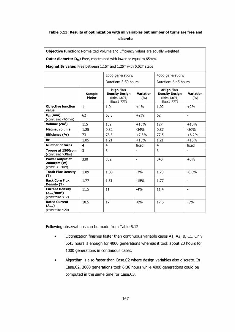
167

Table 5.13: Results of optimization with all variables but number of turns are free and

discrete




2000 generations


4000 generations


Sample Motor


Variation (%)

aHigh Flux Density Design (Bth≤1.89T, Bbc≤1.77T)

Variation (%)


1 1.04 +4% 1.02 +2%

Dso (mm) (constraint <65mm)

62 63.3 +2% 62 -

Volume (cm3) 115 132 +15% 127 +10% Magnet volume 1.25 0.82 -34% 0.87 -30% Efficiency (%) 73 78.3 +7.3% 77.5 +6.2% Br 1.05 1.21 +15% 1.21 +15% Number of turns 4 4 fixed 4 fixed Torque at 1500rpm (constraint >3Nm)

3 3 - 3 -

Power output at 2000rpm (W) (const. >330W)

330 332 - 340 +3%


1.89 1.80 -3% 1.73 -8.5%


1.77 1.51 -15% 1.77 -


11.5 11 -4% 11.4 -


18.5 17 -8% 17.6 -5%


• Optimization finishes faster than continuous variable cases A1, A2, B, C1. Only

6:45 hours is enough for 4000 generations whereas it took about 20 hours for

1000 generations in continuous cases.

• Algortihm is also faster than Case.C2 where design variables also discrete. In

Case.C2, 3000 generations took 6:36 hours while 4000 generations could be

computed in the same time for Case.C3.

168

• Fixing number of turns avoided to go to local minima as observed in Case.C2

and better designs are reached. An objective function 1.02 is reached where it

is 1.10 in Case.C2.

• The objective function could be reduced by a further 2% with 2000 more

generations.

• The final design has 15% larger volume after 2000 generations whereas

volume increase is reduced to 10% at the end of 4000 generations.

• In first run, optimum design efficiency is 7.3% higher than sample motor.

Efficiency decreases in further iterations and is only 6.2% higher after 4000

generations. Note that after this second run volume of the motor is reduced by

5%.

• Magnet Br value is pushed to 1.21 T and magnet volume is considerably lower.

• Power constraint at 2000 rpm and torque constraint at 1500 rpm are satisfied

for both designs.

• Tooth flux density is not pushed to limits; it was 3% lower in the first run and

8.5% lower after 4000 generations. This may be a sign for a need for further

iterations.

• Current density is pushed to towards limit for both designs and rated current

density is selected around 17-18 Arms similar to results of previous cases.

5.6 Convergence Behavior of Optimization Algorithm

To see evolution of the optimized results, design outputs at selected generations of GA

is tabulated in Table 5.14. Number of feasible designs as well as values of minimum and

maximum cost function values are listed for selected generations. The cost function

range is also plotted as shown in Figure 5.11.

The initial population for GA algorithm consist of 100 designs all of which are generated

by modeFrontier as described in Appendix A.4. No feasible designs exist in initial

population. The cost function value diverges between 1.47 at max -2.3 at minimum. The

negative cost function is due to negative efficiency calculated for that design. For some

designs, negative power output values are calculated which results in negative

efficiencies. Of course these designs are marked as unfeasible and next generations are

improved to fit into constraints.

169

Table 5.14: Evolution of designs for high-flux optimization with all design parameters

set free

Number of generation

Number of

feasible designs

Minimum cost

function value for unfeasible designs

Maximum cost

function value for unfeasible designs

Feasible minimum

cost

Feasible maximum

cost

Variation of

feasible designs

Initial population

0 -2,3 1,47 - -

100 0 0,55 1,23 - -

200 0 0,48 1,24 - -

400 0 0,48 1,10 - -

600 5 0,50 1,10 0,971 0,972 ±0.5%

700 23 0,42 1,19 0,968 0,969 ±0.5%

800 6 -4,43 1,13 0,968 0,968 0

900 11 0,41 1,74 0,967 0,967 0

1000 25 0,42 1,20 0,967 0,971 ±2%

Figure 5.11: Evolution of feasible designs high-flux optimization with maximum ordered

design vector

170

Following observations can be made from the presented figure Figure 5.11:

• First feasible designs appear at 600th generation and more feasible designs are

reached in next generations.

• Once a generation with feasible solutions is reached, the variation between

maximum and minimum objective function value for feasible designs is 0.5%

which tells that diversity of feasible designs is very limited. This shows that

optimization algorithm sticks to observed feasible designs very much and new

designs with distinct cost function values are not created.

• Furthermore it can be argued that the the process can be stopped say after

about 600 generations to reduce computer time consumption without sacrificing

much accuracy

• Limited diversity of feasible designs may be due to algorithm parameters which

are set at the beginning of the run. These parameters include cross-over

probability and distribution index for cross-over which are presented in Appendix

A.4 in detail. It may be concluded that values for these control parameters for

GA are conservative and limits diversity of generated population for feasible

designs.

5.7 Conclusions on Optimization Results

Based on the presented observations on optimization results, following commons

conclusions can be made about the optimization:

• Flux densities are mostly pushed to the constraint limits in the designs even it

is low or high. It can be stated that the flux density limits in a design must be

chosen carefully. Preferably maximum feasible flux densities must be set to

have the best design in terms of volume and efficiency.

• Efficiency objective appears to be more dominant than volume objective

although they are equally weighted. This may be because of more parameters

and calculations affecting these objectives. Volume is dependant on

geometrical dimensions, but efficiency depends on geometrical dimensions as

well as magnetic calculations which means that more variables exist in

efficiency calculations.

• Better designs in terms of cost function are obtained when no design variable is

fixed. This states that more efficient optimization is performed when the

171

optimization algorithm is set free to assign values of design parameters. Also it

can be avoided to stick in a local minimum by setting all parameters free.

• Control parameter values for GA are very effective on the diversity of

generated feasible designs. Conservative parameter tuning leads to limited

variation of feasible designs. On the other hand, too much randomness in the

algorithm by setting control parameters liberally may come with need for more

generations to reach designs with cost functions as reached by conservative

parameters. This issue needs further investigation.

• Number of turns for stator winding is selected as 4 in three of the designs

(Case.A1-B-C1) whereas it is selected as 3 in optimization runs with new

population (Case.A2) and discrete variation steps (Case.C2). Investigating the

results with 3 number of turns show that 4 is optimum value. Although 330W

power constraint at 2000rpm is satisfied at defined limit, torque output at

1500rpm is achieved much higher than 3 Nm constraint. The number of turns

affects torque-speed profile at constant power region very much. A design with

3 turns can output 330W output 2000rpm but leads to over-sized torque output

at 1500rpm. This is not the case as observed in Case.A-C-D where

optimizations lead to 4 turns. This shows that if power and/or torque outputs

are not pushed to the constraint limits, than most probably, number of turns or

another parameter with high degree of effect (Number of turns is directly

present in torque and emf equations) in performance calculations is improperly

selected.

• Although discrete optimizations perform faster, there is a possibility of

converging to local minima if algorithm control variables (mutation and cross-

over probability etc.) are not properly set.

172

CHAPTER 6

CONCLUSION

The objective of this thesis work can be summarized as follows:

1. To develop an accurate PM machine model for performance calculations

2. To investigate measurement methods in the literature for PM motor

parameters and performance

3. To conduct selected test methods on the PM motor and determine model

parameters

4. To study reliability of the presented model by performing performance analysis

(e.g. torque-speed) on the model with the measured parameters and compare

calculated performance

5. To propose a set of test methods to fully characterize a PM machine. Any test

method has not been standardized yet.

6. To develop an analytical set of equations to relate motor performance and

parameters to machine dimensions and material properties for optimization

purpose.

7. To study accuracy of developed analytical model by comparing calculated

parameters and performance with measurements

8. To perform optimum design with the developed analytical model

These objectives have been greatly achieved in this work.

In CHAPTER 2, the conventional two-axis electrical model for brushless DC machines is

employed for performance calculations of the sample motor. This model is reviewed in this

chapter. The lumped magnetic circuit model given in the literature is also reviewed.

Calculation of the steady-state motor performance using this equivalent circuit is

discussed.

Accuracy of the model must be studied first by comparing calculated sample motor

performance by utilizing measured parameters; with the measured performance. To

173

achieve a reliable comparison, accurate measurement of the parameters and the motor

performance is necessary. For this reason, a section in CHAPTER 3 is devoted to literature

survey mainly among IEEE Standards and IEEE published papers on measurement of PM

brushless DC motor performance characteristics and two-axis model equivalent circuit

parameters.

It is observed that although many studies are present for internal magnet type PM

machines, there is not much work on surface PM type motors. A group of parameter and

performance test methods has been selected for further investigation.

It is observed that most of the equivalent circuit parameters are simple to measure except

inductance measurement. The measurement of d-q axis inductances of a PM motor is a

challenging issue. Many studies on inductance measurement of PM machines are published

covering various methods. Selected methods from the literature for inductance

measurement are applied on a test motor and results are compared which include:

Inductance measurement at running conditions

Inductance measurement at standstill

Inductance measurement by DC decay tests

Measurements are repeated at different current levels and frequencies, to find out

whether these factors affect inductance.

For d-axis, it is shown that standstill and running tests results agree by 5% and they agree

with manufacturer data for the sample motor by 10%. Results at different frequencies

agree within 3%. Also inductance is almost constant within 5% dispersion with increasing

current. The effect of demagnetizing current on d-axis inductance is also investigated. It is

found that measured inductance is 10% higher than what is found with armature current

in magnetizing direction. This result shows general agreement with the literature.

For q-axis, running and standstill tests results do not agree with manufacturer data. On

the other hand the standstill test result agrees with the manufacturer data.

When investigated it is found that inductance measurements from running tests (load test)

show considerable variation under changing frequency and current. It is observed that q-

axis inductance measurements are largely dependent on accurate load angle

measurement. This is because inductance calculation during running test involves sine of

load angle. Electrical load angle of sample PM motor is about 20-25° at full load,

calculated inductance values become very diverse with even 1° measurement error. On

the other hand, calculated inductances from standstill tests are almost same (only 1%

dispersion) at different currents and frequencies.

174

On the other hand, DC decay tests did not give similar results with both running and

standstill tests for d-q inductances. Also dc decay test results for d-q axes do not agree

with manufacturer data either. Inductance variation trend with current’ for this test, is also

contrary to expectation where a decrease with increasing current was expected due to

possible saturation in magnetic paths.

Standstill tests are concluded to be most proper method for d-q inductance

measurements, because results are reliable, test rig is easy to setup and inductance

calculation from measurement data is simple. Standstill tests are performed by aligning the

rotor to magnetic “d” and “q” axes and exciting the motor terminals. It is also shown that

the excitation scheme (AC sinusoidal or PWM) do not affect results unless fundamental

harmonic of both excitation voltage and induced motor current are used in calculations.

The most valuable contribution of this work is that not much study is available on

measurement of d-q inductances of a surface PM motor. Furthermore, no previous work is

found which covers all test methods at once on the same motor.

Also cogging torque measurement is performed on the sample motor, by driving the motor

by external means, at different speeds. Measured cogging torque values are compared

with FE solution results. It is found that measured cogging torque is 0.2Nm is at most, that

is about 1% of rated torque. On the other hand FE solutions predicted much smaller

cogging torque (0.02). This is possibly because some of the cogging torque is due to

manufacturing problems and because of the test set up irregularities. It is concluded that

cogging torque measurements should be performed at very low speed with high inertia

especially if measured magnitudes are very low. Test at low speed with high inertia on the

shaft enhances the measurement accuracy.

CHAPTER 4 concentrates on the calculation of motor equivalent circuit parameters from

motor dimensions. Once this is done, for a given set of dimensions, the motor

performance can also be calculated. The approach used for parameter calculations is

based on what is available in the literature.

The accuracy of the analytical model is validated by inserting measured parameters to the

model and comparing calculated performance with measured performance. Following

performance calculations are done for performance determination:

Torque-Speed

Power-Speed

Current-Speed

175

No-load losses (friction-windage and core loss) are not calculated in the model, but instead

no-load losses of the sample motor is measured and its variation with speed is obtained. It

is assumed that since the designed motor is similar to sample motor in size and power,

similar no-load loss will exist in the new design. The equation representing no-load loss

variation with speed is used in the new torque output calculations. The equivalent losses

at an operating speed are represented as a decrease in the developed electromagnetic

torque.

Although this approach gave satisfactory results for this thesis work, it may not work for

larger machines where core-losses are more effective in no-load losses. Friction-Windage

losses are dominant because electrical steel body is very small in 0.33kW sample motor.

When larger machines (30-40 kW) are to be designed, core losses may rise to 10% of

rated power and these losses must be accurately calculated for reliable performance

validations. More accurate analytical equations shall be developed based on electrical steel

loss characteristic rather than interpretation of measurements.

A comparison of torque-speed curves are performed based on calculated and measured

characteristic as well as manufacturer data. It is shown that steady state torque can be

calculated within 1% accuracy in constant torque region and with 5% accuracy in constant

power region as shown in Figure 4.27. Having validated the developed analytical model, it

is employed fin the software developed for optimum design of a Surface Mount PM

Machine.

In CHAPTER 5, the software developed for optimum motor design of surface mount PM

motors is described. The application is developed on a commercially available software

platform; modeFrontier. The program includes many optimization algorithms which can be

linked to auxiliary programs such as MATLAB, Excel and Ansys. In this work, no original

optimization algorithm is developed but modeFrontier is linked to the developed MATLAB

script which includes all the set of derived analytical equations developed in CHAPTER 4.

Genetic algorithm (GA) is selected as the optimization algorithm because it needs no initial

feasible designs. The ability of GA for searching optimum design in the entire design space

for variables is also preferred.

The design vector consists of 9 design parameters including Axial length, Slot depth,

Stator yoke height, Tooth width, Diameter at magnet base, Magnet height, magnet arc

span in one pole pitch, turns per coil, magnet Br. It is shown in CHAPTER 4 that all motor

parameters and performance curves can be analytically calculated by these 9 variables.

176

Optimization study is repeated under following conditions to examine their effects on

finding an optimum solution:

Effect of flux density constraints

Importance of initial population on the solution

Assigning discrete variation steps for design variables

Fixing a parameter to reduce the number of independent variables

This study led to the following conclusions:

1. In most of the final designs, flux densities are pushed to defined limits. When

designs with high and low flux density constraints are compared, it can be stated

that volume and efficiency of the final designs are dependent on the flux density

constraints because designs with higher flux densities have lower volume.

Preferably, maximum feasible flux densities must be set to have the best design

in terms of minimum volume with maximum efficiency.

2. Results showed that convergence behaviour of GA algorithm is dependent on

initial population. Different optimum designs were reached with two different

initial populations. It can be recommended that any optimization should be

repeated with different initial designs to determine better of the local minima.

3. It is observed that introducing step changes for design variables (see Section

5.5.5), wherever possible, greatly reduces convergence time. In the study here,

1000 generations in GA was executed in 3:36 hours when discrete variables were

used instead of 20 hours needed with continuous variables. On the other hand,

best designs are reached when all design parameters were continuously varied.

4. Effect of reducing design variables is studied by fixing magnet type, motor outer

diameter and umber of turns per phase one at a time. Results showed that fixing

number of turns may increase the possibility of reaching feasible designs in earlier

generations which leads to smaller objective functions in final design. On the

other hand, fixing outer diameter resulted in worse designs than optimization with

all variables free.

5. Almost the same magnitude of objective function could be reached in final

designs when magnet type was fixed. When magnet type is extracted from design

variables, only geometrical parameters are left as independent variables. It is

interpreted that if the design vector for an optimization consists of similar types of

parameters, better designs can be reached.

177

6. Having investigated final designs of different optimization studies, it can be

concluded that global optimum is not always guaranteed for GA. Control

parameters (such as mutation and cross-over probabilities) are very effective on

ability of the algorithm to converge to a global optimum design. Conservatively

selected control parameters may lead to convergence to local minima. Different

optimization runs may be performed to search for best control parameters for a

specific optimization.

In addition to studied and presented work in this thesis, following topics can be studied

further as a future work:

A more intense core loss calculation can be developed and integrated into

motor design script in MATLAB. It is evident that for larger machines where

core-loss is a major part of losses, the already available equations will not

give accurate results.

Magnets are assumed to be parallel magnetized for all designs. Effect of

magnetization direction variation to magnet shaping is not studied. This can

be included in the developed analytical equations.

Cogging torque calculation is not included in the analytical model.

Torque ripple calculation is not included in the in the developed model.

Instead a constraint is placed on the total harmonic distortion of the air gap

flux density variation. The validity of this approach needs to be investigated.

Different objective functions can be studied to observe optimization algorithm

behaviour. The inclusion of efficiency in the objective function is found to

increase the volume of the final design. It may be worthwhile to investigate

what happens when volume is defined as the sole objective function.

Finite element analysis is not employed in the optimization here. FE can be

included in optimum design process in some manner to increase accuracy of

the magnetic model or to calculate cogging torque.

Only genetic algorithm (GA) is employed in optimization. There are also many

other algorithms such as Simplex, Levenberg-Marquardt and Game theory.

Those can be studied to observe their effect in terms of converge time,

constraint satisfaction, converging to global optimum.

178

REFERENCES

STANDARDS

[1] IEC Pub. 34-4: Methods for determining synchronous machine quantities from tests,

1985.

[2] IEEE Standard 115A: IEEE Standard procedures for obtaining synchronous machine

parameters by standstill response testing, 1987.

[3] IEEE Standard 115-1995, IEEE Guide: Test Procedures for Synchronous Machines,

IEEE Std. 115 ISBN 1-55 937-710-0, 1995.

[4] IEEE Standard 118-1978, “IEEE Standard Test Code for Resistance Measurement”

[5] IEEE Standard 100-2000, “The Authoritative Dictionary of IEEE Standards Terms”,

Seventh Edition, 2000.

BOOKS

[6] T.J.E. Miller, “Brushless Permanent-Magnet and Reluctance Motor Drives”, Claredon

Press, Oxford University Press, 1989.

[7] J.F. Gieras, M.Wing, “Permanent Magnet Motor Technology – Design and

Applications”, 2nd Ed., Marcel Dekker Inc., New York, ISBN: 0-8247-0739-7, 2002.

[8] D. Hanselman, “Brushless Permanent Magnet Motor Design”, 2nd Ed., The Writers’

Collective, ISBN:1-932133-63-1, 2003.

[9] T.A. Lipo, “Introduction to AC Machine Design”, Vol.1, Wisconsin Power Electronics

Research Center, University of Wisconsin, 1996.

[10] G. Henneberger, Lecture Notes on “Electrical Machines II - Dynamic Behavior,

Converter Supply and Control”, Aachen University, Rev.2, July 2003.

[11] P Eykhoff, “System identification, parameters and state estimation”, Wiley, 1974.

PUBLISHED PAPERS

[12] F. W. Merrill, “Permanent-Magnet Excited Synchronous Motors”, Transactions of the

AIEE Power Apparatus and Systems, Vol. 73, Issue 2, Part III-B, Jan 1954.

[13] T.J.E. Miller, “Methods for Testing Permanent Magnel Polyphase AC Motors”, IEEE

IAS Conference Record, pp.494-499, 1981.

179

[14] B.J. Chalmers, S.A. Hamed, G.D. Baines, “Parameters and performance of a high-

field permanent-magnet synchronous motor for variable-frequency”, IEE Proceedings,

Vol.132, Pt. B, No.3, pp.117-124, May 1985.

[15] A. Consoli, A. Raciti, “Parameter Analysis of Permanent Magnet Synchronous

Machines”, IEEE Trans. on Industry Applications, Vol.2, Issue.2, pp.350-354, Mar/Apr

1991.

[16] P. H. Mellor, F. B. Chaaban, K. J. Binns, “Estimation of parameters and performance

of rare-earth permanent-magnet motors avoiding measurement of load angle", IEE

Proceedings-b, Vol.138, Issue.6, pp.322-330, Nov 1991.

[17] B. Stumberger, B. Kreca, B. Hribernik, “Determination of Parameters of Synchronous

Motor with Permanent Magnets from Measurement of Load Conditions”, IEEE Transactions

on Energy Conversion, Vol.14, No.4, pp.1413-1416, Dec 1999.

[18] Fidel FB, Aurelio GC, R. Faure, “Determination of Parameters in Interior Permanent-

Magnet Synchronous Motors with Iron Losses without Torque Measurement”, IEEE

Transactions On Industry Applications, Vol. 37, No. 5, pp.1265-1272, Sep/Oct 2001.

[19] J.F. Gieras, E. Santini, M. Wing, “Calculation of synchronous reactances of small

permanent-magnet alternating-current motors: comparison of analytical approach and

finite element method with measurements”, IEEE Transactions on Magnetics, Volume 34,

Issue.5, Part.2, pp.3712-3720, Sep 1998.

[20] M. A. Rahman, M. A. Jabbar, P. Zhou, “Field Circuit Analysis of Permanent Magnet

Synchronous Motors”, IEEE Transactions On Magnetics, Vol. 30, No. 4, pp.1350-1359, Jul

1994.

[21] P. Pillay, R. Krishnan, “Application Characteristics of Permanent Magnet

Synchronous and Brushless dc Motors for Servo Drives”, IEEE Transactions on Industry

Applications, Vol. 21, No. 5, pp.986-996, Sep 1991.

[22] P. Pillay, P. Freere, “Literature Survey of Permanent Magnet AC Motors and Drives”,

IEEE Conference Record of the Industry Applications Society Annual Meeting, pp.74-84,

1989.

[23] A. Binder, T. Schneider, “Permanent magnet synchronous generators for

regenerative energy conversion - A Survey”, European Conference on Power Electronics

and Applications, pp.10, Sep 2005.

[24] R.S. Colby, “Classification of Inverter Driven Permanent Magnet Synchronous

Motors”, Industry Applications Society Annual Meeting, Vol.1, pp.1-6, 1988.

180

[25] R. Mizutani, T. Takeshita, N. Matsui, “Current model-based sensorless drives of

salient-pole PMSM at low speed and standstill”, IEEE Transactions on Industry

Applications, Vol.34, Issue.4, pp.841-846, July 1998.

[26] S. Bolognani, R. Oboe, M. Zigliotto, “Sensorless full-digital PMSM drive with EKF

estimation of speed and rotor position”, IEEE Transactions on Industrial Electronics,

Vol.46, Issue.1, pp.184-191, Feb 1999.

[27] S. Morimoto, K. Kawamoto, M. Sanada, Y. Takeda, “Sensorless Control Strategy for

Salient-Pole PMSM Based on Extended EMF in Rotating Reference Frame”, IEEE

Transactions On Industry Applications, Vol. 38, No. 4, pp.2637-2644, July/Aug 2002.

[28] A.H. Wijenayake, P. Schmidt, “Modeling and Analysis of Permanent Magnet

Synchronous Motor by Taking Saturation and Core Loss into Account”, Proc. of Int. Conf.

on Power Electronics and Drive Systems, Vol.2, pp.530-534, May 1997.

[29] T. Kenjo, S. Nagamori, “Permanent Magnet and Brushless DC Motors”, Claredon

Press, Oxford University Press, 1985.

[30] K.J. Overshott, “Magnetism: it is permanent”, IEE Proceedings-A, Vol. 138, No.1,

pp.22-30, Jan 1991.

[31] N. Urasaki, T. Senjyu, K. Uezato, “Automatic Parameter Measurement for Permanent

Magnet Synchronous Motors Compensating Dead Time Effect”, Proc. of the 2002 IEEE Int

Symposium on Industrial Electronics, Vol.3, pp.717-722, 2002.

[32] T. Senjyu, Y. Kuwae, N. Urasaki, K. Uezato, “Accurate parameter measurement for

high speed permanent magnet synchronous motors”, IEEE 32nd Annual Power Electronics

Specialists Conference, Vol.2, pp.772-777, 2001.

[33] J. P. Wang, D. K. Lieu, W. L. Lorimer, and A. Hartman, “Comparison of Lumped

Parameter and Finite Element Magnetic Modeling in a Brushless DC Motor”, IEEE

Transactions On Magnetics, Vol. 33, No. 5, Part.2, pp.4092-4094, Sep 1997.

[34] Qu Ronghai, M. Aydin, T.A. Lipo, “Performance comparison of dual-rotor radial-flux

and axial-flux permanent-magnet BLDC machines”, IEEE International Electric Machines

and Drives Conference, Vol.3, pp.1948-1954, 2003.

[35] K.J. Strnat, “Modern Permanent Magnets for Applications in Electro-Technology”,

Proc. of the IEEE, Vol.78, No.6, pp.923-946, June 1990.

[36] M.A. Jabbar, J. Dong, Z. Liu, “Determination of Parameters for Internal Permanent

Magnet Synchronous Motors”, IEEE Int. Conf. on Electric Mach and Drives, pp.149-156,

2005.

181

[37] V.Z. Groza, M. Biriescu, G. Liuba, “Measurement of reactance of synchronous

machines at standstill”, IEEE Int. Conf. on Elec. Mach. and Drives (IEMD, pp.171-173 ),

May 1999.

[38] B. Stumberger, B. Kreca, B. Hribernik, “Determination of Parameters of Synchronous

Motor with Permanent Magnets from Measurement of Load Conditions”, IEEE Transactions

on Energy Conversion, Vol. 14, No. 4, pp.1413-1416, Dec 1999.

[39] M. A. Rahman, P. Zhou, “Accurate determination of PM motor parameters by digital

torque angle measurement”, Journal of Appl. Physics, Vol.76, No.10, pp.6868-6870, 1994.

[40] D. Iles-Klumpner, I. Boldea, “Comprehensive Experimental Analysis of the IPMSM

for Automotive Applications”, 12th International Power Electronics and Motion Control

Conference, pp.1776-1783, 2006.

[41] F.W. Carter, “Note on air gap and interpolar induction”, Journal of Proceedings of

the Institution of Electrical Engineers, Part 146, Vol.29, pp.925-933, 1900.

[42] S.F.Gorman, C.Chen, J.J. Cathey, “Determination of Permanent Magnet Synchronous

Motor Parameters for Use in Brushless DC Motor Drive Analysis”, IEEE Transactions on

Energy Conversion, Vol.3, No.3, pp.674-681, Sep 1988.

[43] S. Yamamoto, T. Ara, S. Oda, K. Matsuse, “Prediction of starting performance of PM

motors by DC decay testing method”, IEEE Transactions on Industry Applications, Vol.36,

Issue.4, pp.1053-1060, July/Aug 2000.

[44] R. Dutta, M.F. Rahman, “A Comparative Analysis of Two Test Methods of Measuring

d-q Axes Inductances of Interior Permanent-Magnet Machine”, IEEE Transactions on

Magnetics, Vol.42, Issue.11, pp.3712-3718, Nov 2006.

[45] F. Deng, “An improved iron loss estimation for permanent magnet brushless

machines”, IEEE Transaction on Energy Conversion, Vol.14, Issue.4, pp.1391-1395, Dec

1999.

[46] KC Kim, J. Lee, HJ Kim, DH Koo, “Multiobjective Optimal Design for Interior

Permanent Magnet Synchronous Motor”, IEEE Transactions On Magnetics, Vol. 45, No. 3,

pp.1780-1783, March 2009.

[47] N. Boules, “Design Optimization of Permanent Magnet DC Motors”, IEEE

Transactions on Industry Applications, Vol. 26, No. 4, pp.786-792, July/Aug 1990.

[48] L. Tutelea, I. Boldea, “Optimal Design of Residential Brushless d.c. Permanent

Magnet Motors with FEM Validation”, ACEMP 2007, pp.435-439, 2007.

182

[49] N. Bianchi, S. Bolognani, “Brushless Dc Motor Design: An Optimisation Procedure

Based on Genetic Algorithms”, EMD Conference Publication, No. 444, pp.16-20, 1997.

[50] Y. Duan, R.G. Harley, T.G. Habetler, “Method for Multi-objective Optimized Designs

of Surface Mount Permanent Magnet Motors with Concentrated or Distributed Stator

Windings”, Proceedings of IEMDC 2009, pp.323-328, 2009.

[51] W. Ouyang, D. Zarko, T.A.Lipo, “Permanent Magnet Machine Design Practice and

Optimization”, Industry Applications Conference, IAS 2006, pp.1905-1911, 2006.

[52] R. Wrobel, P. H. Mellor, “The use of a genetic algorithm in the design optimisation

of a brushless DC permanent magnet machine rotor”, PEMD 2004, No.498, pp.823-827,

2004.

[53] T. J. Vyncke, F. M. De Belie, R. K. Boel, J. A. Melkebeek, Y. Cheng, P. Lataire,

“Identification of PM Synchronous Machines in the Frequency Domain by Broadband

Excitation”, International Symposium on Power Electronics, Electrical Drives, Automation

and Motion (SPEEDAM), pp.1253-1258, 2008.

[54] K. Deb, A. Pratap, S. Agarwal, T. Meyarivan, ” A Fast and Elitist Multiobjective

Genetic Algorithm: NSGA-II”, IEEE Transactions on Evolutionary Computation, Vol.6, No.2,

April 2002.

INTERNET WEB-SITES

[55] Wikipedia, Magnet, “http://en.wikipedia.org/wiki/Four_Great_Inventions_of_

Ancient_China”, Last visited on Nov 27, 2008.

[56] IBS Magnet, “Permanent Magnets – Materials and Magnet Systems”,

“http://www.ibsmagnet.de”, Last visited on Dec 14, 2007.

[57] Ningbo Ketian Magnet Co Magnet, “http://www.kt-magnet.com”, Last visited on

June 20, 2009.

[58] ESTECO, “http://www.esteco.com”, Last visited on July 10, 2009.

[59] JFE Steel Corporation, “http://www.jfe-steel.co.jp/en/”, Last visited on Aug 15,

2008.

MANUALS

[60] modeFrontier® 4 User Manual, ESTECO

183

APPENDIX

A.1 MATLAB Code of Analytical Calculation Program

Main Program

eval('p1_IndependentVariables') %take independent variables % in optimization program, these variables are assigned by the modeFrontier % itself. You have to remove this line to call for independet variables. eval('p2_Assumptions_Definitions') %define assumptions eval('p3_Dimensions') %calculate stator and rotor dimensions eval('p4_Electrical_Parameters') %calculate electrical parameters such as "Rs, Lq" eval('p5_Magnetic_Circuit_Calculations') %calculate magnetic parameters such as "kemf, ktorq" eval('p6_reference_calculations') %calculations at reference speed eval('p7_matrix_form') %matrix form %% GRAPH PLOTINGS % experiment torque-speed data [500 1600 1800 2000 2280 2730],[3 3 2.55 2.35 1.8 0.6] %subplot(2,1,1),plot(w,maxTe,'m--',w,ratedTe,'b'),grid,ylabel('Torque (Nm)'),xlabel('Speed (rpm)'),title('Torque-Speed'),%axis([0 3500 0 4]) %subplot(2,1,2),plot(w,maxIt,'m--',w,ratedIt,'b-'),xlabel('speed (rpm)'),ylabel('Current (Arms)'),grid,%axis([0 3500 0 40])

“p1_IndependentVariables” Module

Br = 1.05; %magnet remanent flux density Lsta = 38e-3; %axial length of magnetic circuit h1 = 8.275e-3; %slot depth (check drawings) hbc = 2.25e-3; %back-core depth (check drawings) g = 0.75e-3; %airgap (check drawings) Wth = 1.82e-3; %Tooth width (check drawings) Dmb = 26.2e-3; %diameter at magnet base. Draw a circle touching the magnet bottom %which is centered in the center of the rotor. This is the diameter of that circle. alfa = 0.748; %magnet pitch / pole pitch %angular span of magnet with respect to total pole pitch. The angle that %mnagnet covers. hmag = 3.65e-3; %magnet maximum height in the middle Nturn = 4; %turns per coil.

“p2_Assumptions_Definitions” Module

w = 1:20:3501; %Speed step in rpm for calculations Imax = 35; %Current Limit in Arms. already defined by inverter Vline = 21; %bus voltage of inverter pole = 8; %Motor pole number Nslot = 27; %slot number of stator phase = 3; %number of phase Kstack = 0.985; %“Stacking factor” kfill = 0.339; %Slot fill factor Cu_rho = 59.6e-6; %Copper conductivity (Siemens/m) muR = 1.05; %Magnet muR magnet_muR =1.05; %ignore it for this time prl = 0.1; %Rotor leakage factor between adjacent magnets w0 = 1.27e-3; %Slot opening width (meters) - check drawings h0 = 0.8e-3; %Slot opening depth (meters) - check drawings mu0 = 4e-07*pi; %“space air permeability” - Henry /m Ncoil = 9; %Coils per phase, this is fixed for a defined slot number Coilpitch = 16/18; %Coil pitch of the winding. We have concentrated winding. kw = 0.94; %winding factor- precalculated from the distribution.

“p3_Dimensions” Module

%Airgap calculations (above magnet) %magnet is divided into five pieces. Check ilker's thesis for details.

184

g1= g; %airgap at magnet surface tip. at max magnet height g2= g / cos(1*alfa/4); %airgap at magnet second region g3= g / cos(2*alfa/4); %airgap at magnet side %Stator dimensions Dms = Dmb+2*hmag; %Diameter at magnet surface (meters) Dmq = Dmb+2*hmag-2*1e-3; %Diameter at surafece of saliency between magnets (meters) Dsi = Dmb+2*(hmag+g); %Diameter at stator inner surface (meters) %Magnet dimensions teta = alfa*360/pole; %Angle span of magnet at magnet surface Wmag = Dms*sind(teta/2); %Width of magnet dip (meters) hm2= hmag-0.5*(Dms-Dms*cosd(teta/4)); %mean magnet height at region 2 hm3= hmag-0.5*(Dms-Dms*cosd(teta/2)); %mean magnet height at regions 3 hmagmean = hm3+(hmag-hm3)*2/pi; %overall mean magnet height Apole = pi*(Dsi-g)*Lsta/pole; %Total pole area (m^2) Amag = Wmag*Lsta; %Magnet cross sectional area at magnetization direction (m^2) Ag = (Wmag+2*g)*(Lsta+2*g); %Airgap area including fringing flux (m^2) %Stator dimensions (Refer to drawings) w1 = (Dsi+2*h0)*pi/Nslot-Wth; %slot width near to slot opening (meters) w2 = (Dsi+2*h0+2*h1)*pi/Nslot-Wth; %slot width at slot dip (meters) h2 = w2/2; %tooth height (meters) hslot = h0+h1+h2; %Total slot height (meters) Aslot = (w1+w2)/2*h1 + pi*0.5*h2^2; %Total slot area (m^2) Abc = hbc*Lsta; %back core cros sectional area (m^2) Ath = Wth*Lsta; %Tooth cross sectional area (m^2) Dso = Dsi + 2*hslot+2*hbc; %Stator outer diameter (meters) Vol = pi*(0.5*Dso)^2*Lsta; %total volume stator+rotor (m^3) Surface = 4*Dso*Lsta + 2*Dso^2; %Total surface area for heat transfer (m^2) Rth = 1/(58.229*Surface); %Thermal resistance (oC/Watt) - from MOOG datasheet Dwire = 2*sqrt(Aslot/2*kfill/Nturn/pi); %winding wire diameter rotortest = 0.5*((Dmb-Wmag)/sqrt(2)-Wmag); %Distance between bottom tip of two adjacent magnets %to check interference Mdens = 7.65e3; %density of lamination kg/m3 Mth = Nslot*hslot*Wth*Lsta; %Total mass of tooth lamination Mbc = hbc*Lsta*pi*(Dso-hbc); %Total mass of back-core lamination Mrot = (0.5*Dmb)*(tan(2*pi/pole/2)*0.5*Dmb); %Total mass of rotor roke Mtot = Mdens*(Mth+Mbc+Mrot); %Total mass of stator yoke

“p4_Electrical_Parameters” Module

%Electrical parameters slotMatrix = [0 0 0 0 0 0; 9 15 18 21 24 0; 0 0 0 0 0 0; 18 21 27 30 33 36]; %matrix for available slot numbers for 4 and 8 pole motors with sinusoidal back EMF slotpitchMatrix =[0 0 0 0 0 0; 2 3 4 5 6 0; 0 0 0 0 0 0; 2 2 3 3 4 4]; % matrix for available slot pitches for defined slot numbers Spitch = (slotMatrix(pole/2,:)==Nslot)*(slotpitchMatrix(pole/2,:))'; %selected slot pitch Cpitch = Spitch/(Nslot/pole); %selected coil pitch Ncoil = Nslot/phase; %Number of coils q1 = Nslot/pole/phase; %Slots per pole per phase % Carter coef. calculation (refer to drawings) bo2 = w0; %slot opening width To2 = pi*Di/Nslot; %one slot pitch carter2 =To2/(To2 -bo2^2/(bo2+5*g3)); %carter coefficent %Winding resistance calculation Awire = pi*(0.5*Dwire)^2; %winding wire cross sectional area Lwire = 2*Ncoil*(Lsta+0.01+(Spitch/Nslot*(Dsi+hslot)*pi)); %Total wire length 0.01 is assumption for end winding height. Lcon = (Dsi+hslot)*pi + 2*Ncoil*0.01; %total length of connections between coils Rs = Nturn*(Lwire+Lcon)/Cu_rho/Awire; %Total phase resistance at 25oC Rs = 1.44*Rs; %Total phase resistance at 150oC pT1 =0.5*mu0*(0.623+h0/w0); %Calculated leakage permeances pT2 =mu0/3*h2/w2; %to be cited after

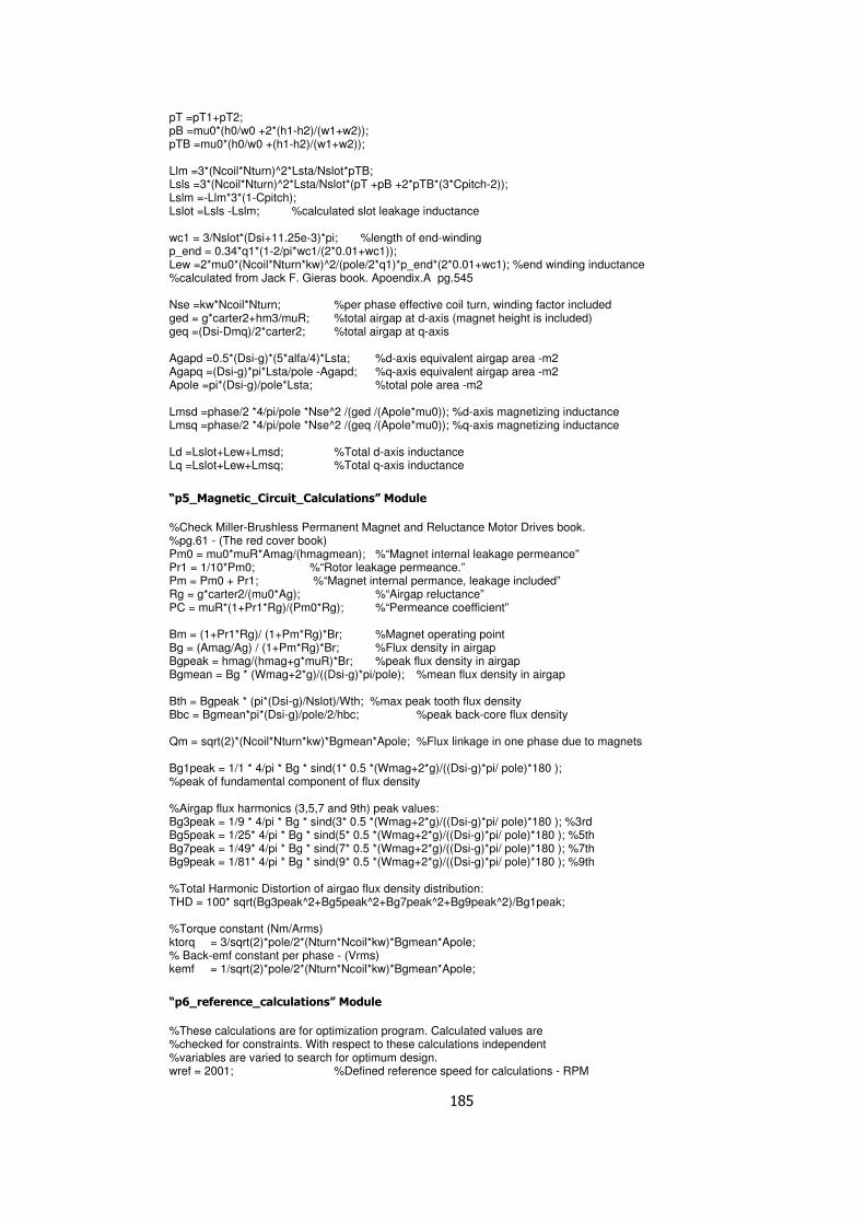
185

pT =pT1+pT2; pB =mu0*(h0/w0 +2*(h1-h2)/(w1+w2)); pTB =mu0*(h0/w0 +(h1-h2)/(w1+w2)); Llm =3*(Ncoil*Nturn)^2*Lsta/Nslot*pTB; Lsls =3*(Ncoil*Nturn)^2*Lsta/Nslot*(pT +pB +2*pTB*(3*Cpitch-2)); Lslm =-Llm*3*(1-Cpitch); Lslot =Lsls -Lslm; %calculated slot leakage inductance wc1 = 3/Nslot*(Dsi+11.25e-3)*pi; %length of end-winding p_end = 0.34*q1*(1-2/pi*wc1/(2*0.01+wc1)); Lew =2*mu0*(Ncoil*Nturn*kw)^2/(pole/2*q1)*p_end*(2*0.01+wc1); %end winding inductance %calculated from Jack F. Gieras book. Apoendix.A pg.545 Nse =kw*Ncoil*Nturn; %per phase effective coil turn, winding factor included ged = g*carter2+hm3/muR; %total airgap at d-axis (magnet height is included) geq =(Dsi-Dmq)/2*carter2; %total airgap at q-axis Agapd =0.5*(Dsi-g)*(5*alfa/4)*Lsta; %d-axis equivalent airgap area -m2 Agapq =(Dsi-g)*pi*Lsta/pole -Agapd; %q-axis equivalent airgap area -m2 Apole =pi*(Dsi-g)/pole*Lsta; %total pole area -m2 Lmsd =phase/2 *4/pi/pole *Nse^2 /(ged /(Apole*mu0)); %d-axis magnetizing inductance Lmsq =phase/2 *4/pi/pole *Nse^2 /(geq /(Apole*mu0)); %q-axis magnetizing inductance Ld =Lslot+Lew+Lmsd; %Total d-axis inductance Lq =Lslot+Lew+Lmsq; %Total q-axis inductance

“p5_Magnetic_Circuit_Calculations” Module

%Check Miller-Brushless Permanent Magnet and Reluctance Motor Drives book. %pg.61 - (The red cover book) Pm0 = mu0*muR*Amag/(hmagmean); %“Magnet internal leakage permeance” Pr1 = 1/10*Pm0; %“Rotor leakage permeance.” Pm = Pm0 + Pr1; %“Magnet internal permance, leakage included” Rg = g*carter2/(mu0*Ag); %“Airgap reluctance” PC = muR*(1+Pr1*Rg)/(Pm0*Rg); %“Permeance coefficient” Bm = (1+Pr1*Rg)/ (1+Pm*Rg)*Br; %Magnet operating point Bg = (Amag/Ag) / (1+Pm*Rg)*Br; %Flux density in airgap Bgpeak = hmag/(hmag+g*muR)*Br; %peak flux density in airgap Bgmean = Bg * (Wmag+2*g)/((Dsi-g)*pi/pole); %mean flux density in airgap Bth = Bgpeak * (pi*(Dsi-g)/Nslot)/Wth; %max peak tooth flux density Bbc = Bgmean*pi*(Dsi-g)/pole/2/hbc; %peak back-core flux density Qm = sqrt(2)*(Ncoil*Nturn*kw)*Bgmean*Apole; %Flux linkage in one phase due to magnets Bg1peak = 1/1 * 4/pi * Bg * sind(1* 0.5 *(Wmag+2*g)/((Dsi-g)*pi/ pole)*180 ); %peak of fundamental component of flux density %Airgap flux harmonics (3,5,7 and 9th) peak values: Bg3peak = 1/9 * 4/pi * Bg * sind(3* 0.5 *(Wmag+2*g)/((Dsi-g)*pi/ pole)*180 ); %3rd Bg5peak = 1/25* 4/pi * Bg * sind(5* 0.5 *(Wmag+2*g)/((Dsi-g)*pi/ pole)*180 ); %5th Bg7peak = 1/49* 4/pi * Bg * sind(7* 0.5 *(Wmag+2*g)/((Dsi-g)*pi/ pole)*180 ); %7th Bg9peak = 1/81* 4/pi * Bg * sind(9* 0.5 *(Wmag+2*g)/((Dsi-g)*pi/ pole)*180 ); %9th %Total Harmonic Distortion of airgao flux density distribution: THD = 100* sqrt(Bg3peak^2+Bg5peak^2+Bg7peak^2+Bg9peak^2)/Bg1peak; %Torque constant (Nm/Arms) ktorq = 3/sqrt(2)*pole/2*(Nturn*Ncoil*kw)*Bgmean*Apole; % Back-emf constant per phase - (Vrms) kemf = 1/sqrt(2)*pole/2*(Nturn*Ncoil*kw)*Bgmean*Apole;

“p6_reference_calculations” Module

%These calculations are for optimization program. Calculated values are %checked for constraints. With respect to these calculations independent %variables are varied to search for optimum design. wref = 2001; %Defined reference speed for calculations - RPM

186

wrad = wref/60*2*pi; %Reference speed in rad/s fe = wref/60*(pole/2); %Electrical operating frequency at reference speed Xq = Lq*2*pi*fe; %Xq reactance at reference speed to be used in electrical equivalent %circuit. Current is to be calculated. emfrpm = wrad*kemf; %Induced EMF voltage per phase in Vrms Vtrpm_ = zeros(1,500); %Dummy matrix filled with zeros for i=1:500 Vtrpm_(i)= sqrt( (emfrpm+ i/10*Rs)^2 + (i/10*Xq)^2 ); %At selected speed, current is increased by steps and we calculate %required terminal voltage for that condition. end % Limiter Vtrpm_( Vtrpm_ > (Vline/sqrt(3)/sqrt(2)) ) = 0; %Eliminating cells above limited bus voltage at reference speed Irpm = length(Vtrpm_(Vtrpm_~=0))/10; %Max current at reference speed after elimination Jcurref = Irpm*Nturn/(Aslot/2*kfill)*10^(-6); %Current density - Arms/mm2 Irated=Irpm; %Rated current is equal to the max current at reference speed %Core-loss calculations %Ref: Fang Deng,"An Improved Iron Loss Estýmatýon For Permanent Magnet Brushless Machines" %IEEE Transactions on Energy Conversion, Vol. 14, No. 4, December 1999 %refer to the reference paper for defined constants in equations ke = 0.2; kh = 0.5; kexc = 0.25; rhot = 0; alfatt = 2*pi*pole/2 /Nslot; Betam = pi*(1-alfa); Pironref = ( kh*fe*Bth^2 + ke*fe^2*Bth)*Mth + ( kh*fe*Bbc^2 + ke*fe^2*Bbc^2)*Mbc; %At this step we have calculated iron loss for every operating frequency %or equivalently for every speed. Pcuref = 3*Irpm^2*Rs; %Copper loss at reference speed for the maximum current available Plossref = Pironref+Pwindref+Pcuref; %Total loss at ref. speed %iron loss + windage loss + copper loss

“p7_matrix_form” Module

% Calculations in matrix form f = w./(60*2/pole); %Conversion of speed steps to electrical operating frequency for calculations Xq = Lq*2*pi*f; %q-axis reactance Xq at every operating frequency % emf = (w/60*2*pi)*kemf; %Induced emf per phase in Vrms Vt_=zeros(Imax*20,length(w)); %Dummy voltage matrix filled with zeros. x-axis is speed, y-axis is current It_=zeros(20*Imax,length(w)); %Dummy current matrix filled with zeros. x-axis is speed, y-axis is current for rw=1:(20*Imax) %for every current step of 0.05Arms for clmn=1:length(w) %for every speed step of 0.06rad/s Vt_(rw,clmn)= sqrt( (emf(clmn)+ rw/20*Rs)^2 + (rw/20*Xq(clmn))^2 ); %required bus voltage is calculated end It_(rw,1:length(w)) = rw/20; %assign current value to current matrix end % Limitations Vlim = (Vt_>=0).*(Vt_<=(Vline/sqrt(3)/sqrt(2))); %Eliminate points in votage and current matrix refering to voltage values over fixed bus voltage Vline Vmatrix = Vlim.*Vt_; %limited voltage matrix. Over voltage values are replaced with zeros. maxVt = max(Vmatrix,[],1); %Terminal voltage at each speed step for max current Imatrix = Vlim.*It_; %terminal current at each speed step Iratedlim = (It_>0).*(It_<=Irpm).*Vlim; %Rated current level limit ratedIt = max((It_.*Iratedlim),[],1); %Rated current level % % Losses Twind = (0.0025*(w/60).^2 + 0.0889*(w/60))./(w/60*2*pi); %“windage+friction” loss for entire speed range maxIt = max(Imatrix,[],1); %Max current at each speed step maxTe = maxIt*ktorq -Twind; %Net torque output at each speed step ratedTe = ratedIt*ktorq -Twind; %Rated torque at each speed step

187

A.2 Matrix Operations in Design Program in MATLAB

At every 100rpm step in full speed range and every 0.5Arms step in current range, the

motor model will be solved to determine motor performance data such as torque, power,

loss, efficiency etc. The defined step in speed range results in 36 operating speeds and

current step results in 70 steps in entire current range.

A.2.1 Voltage and Current Matrices

Considering the specified calculation points in previous section, we have 2520 operating

conditions (36 speed steps x 70 current steps) to solve previously discussed equations.

One approach may be solving electrical and magnetic equivalent circuit for one operating

point and look for the result. However, since we have a powerful calculation tool like

MATLAB, we can solve all equations related to motor performance in once for the entire

operation range. MATLAB has the capability of performing matrix operations very fast. If

proper matrices can be formed, MATLAB can solve the whole problem in a few seconds.

As stated we have 36 operating speed points and 70 current steps. To represent all

operating points, we can use 70x36 matrices in all equations. Using matrices will allow us

to compute all equations at the same time.

In this section, matrices representing induced emf voltage due to magnets and terminal

currents to drive motor are formed. Throughout the whole simulation program calculations

are performed as matrix manipulations since MATLAB responds much faster with matrices.

A.2.2 EMF Matrix

The emf matrix |Et| is formed by calculating generated EMF in the motor for each speed

step. For each speed step, emf constant ke is multiplied by the operating speed. In fact

EMF matrix is an array rather than a matrix because it has one dimension referring to

speed steps. However, to perform matrix operations, we need also second dimension

which corresponds to current steps. For this purpose, the EMF array is cloned 70 times to

form a 70 x 36 array. The resultant emf matrix (Figure A.1) consists of 70 identical rows

which has emf voltage values for each speed step.

188

e1-1 e1-2 … e1-36

e2-1 . . .

. . . .

e70-1 . . e70-36

Figure A.1: EMF matrix |Et| for MATLAB calculation

For example, in “e1-1” is the back emf magnitude when speed is 1rpm and “e1n” is emf at

3501rpm. As stated the values in the same column is identical such that e1-1,e2-1 and

e70-1 are all same which is emf calculated at 1rpm. Equivalently e1-36 and are e70-36 emf

calculated at 3501rpm with equation (a-1).

π260

35013670361 ×== −− ekee (a-1)

A.2.3 Current Matrix

Similar to voltage matrix, current matrix |It| is formed by 36 similar columns which consist

of 70 cells representing terminal current step.

0.5Arms 0.5Arms … 0.5Arms

1.0Arms . . .

1.5Arms . . .

. .

35.0Arms . . 35.0Arms

Figure A.2: Current matrix |It| for MATLAB

A.2.4 Matrix Calculations

We now have formed voltage and current matrices that will be used in equation (a-2). This

equation is based on the phase diagram of the motor operating under vector control which

is presented in Figure 3.29 in Chapter 3.3.3. With this equation, terminal voltage matrix is

189

formed which will include the required bus voltage values for all operating conditions (36

speed steps, 70 current steps).

( ) ( )[ ]2

122

qetphtot LwIRIEV ++= (a-2)

In the above equation, Eo is per phase back emf rms voltage at operating speed, It is

phase rms current, Rph is per phase resistance we is electrical operating speed in rad/s

which can be calculated with equation (a-3);

22

60

pNwe ×= π (a-3)

where “N” is operating speed in rpm and “p” is motor pole number.

By equation (a-2), Vt is calculated for all operating points and a terminal voltage matrix |Vt|

is formed which is also a 36x70 matrix as voltage and current matrices. After that |Vt| is

checked for voltage limitation violation that is each cell value in the matrix is compared

with bus voltage limit (21Vpeak line-line or 8.57Vrms per phase in this thesis work) for

terminal voltage.

To understand this better, consider the following example. Assume that motor is operating

at speed 2000rpm with 30Arms terminal current. The back emf voltage at this speed is;

phaseperVrpmV

E rms

peak

e 6260

2000

23

070.0=×= π (a-4)

where 0.070 Vpeak.s/rad is measured line emf voltage constant of tested motor is divided

by √3 and √2 to get per phase rms voltage. Now let’s solve equation (a-2) at this

operating point.

( )

rms

rmsrmsrmst

V

mHpolesrpm

AohmAVV

70.8

133.02

82

60

200030070.0306

2

12

2

=

×+⋅+= π

(a-5)

Remembering phase voltage limit as 21Vpeak at motor terminals and 8.57Vrms per phase,

the calculated terminal voltage 8.70Vrms is over the limitation that is available 21V bus

voltage is not enough to operate the motor at 2000rpm with 30Arms terminal current. So

we can conclude that this operating point (2000rpm, 30Arms) is unrealizable, no further

calculation (torque,power, etc.) must be done, the value of this cell can be overwritten

with zero not to include in calculations.

190

A.2.5 Matrix Operations

By solving equation (a-2) for all operating conditions, the terminal voltage matrix |Vt| is

formed. In this part we try to trim the formed matrices with respect to current and voltage

limitations. As previously presented, there are invalid operating points where no

performance calculations must be done. It should be checked that motor terminal voltage

remains within limits for each step.

In the terminal voltage matrix, all cells having a value larger than 8.57Vrms are equated to

zero. Also those cells also marked in current matrix, not to solve any torque, power or

efficiency at that point. For example check following sample current and voltage matrices

|It| and |Vt|.

The values in the cells are arbitrarily assigned which are not based on calculations. If

8.57Vrms bus voltage limitation is applied to voltage matrix then the resultant will be as

follows.

191

As it can be noted, the cells with values larger than 8.57Vrms are overwritten with zeros.

Exactly same cells in the current matrix must also be overwritten with zeros.

After eliminating invalid cells, any calculation can be done with any considerations. For

example we can look for pull-out torque of motor, or torque at a specific current. The

torque is calculated by multiplying each cell in the current matrix |It| with torque constant

kt. The resultant is torque matrix |Ttorq|.

192

A.3 Voltage and Current Waveforms of Servo-Motors [10]

Permanent-field (PM = permanent-magnet, permanent-field) synchronous machines can

be operated in different ways. In block-operation, the motor is supplied with rectangular

block) currents and the distribution of the air-gap flux density is rectangular. If the motor

is supplied with sinusoidal currents and the rectangular distribution of the air-gap flux

density is retained, then we have mixed operation. In sinusoidal operation, the current and

the distribution of the air-gap flux are sinusoidal. The figure shows the characteristics of

flux density, current and voltage.

If a machine is operated in block-operation, then it is also called brushless or electrically

commutated DC machine. If a machine is operated in sinusoidal operation, it is also called

self-controlled synchronous machine. The operational performance of permanent-field

synchronous machines with rotor position encoder generally corresponds to the

operational performance of DC machines.

If the machine is supplied with sinusoidal currents, sinusoidal induced voltages are

necessary. We can obtain a nearly sinusoidal air-gap field using parallel magnetized

instead of radial magnetized permanent magnets and by designing a suitable stator

winding (chording for example).

Another possibility is to supply the machine with rectangular (block) currents. The total

supply current has a constant magnitude and is distributed cyclic to the three stator

phases, which results in current blocks with an electrical length of 120° and dead times of

60°. If the induced voltage during the length of a current block is constant, then power of

the phase is constant too. During the dead times the induced voltage has no influence on

the torque generation. The trapezoidal characteristic of the induced voltage results from

q>1 and because of the skewing of the stator slots of one slot pitch.

The advantages of the rectangular supply in comparison to the sinusoidal supply are a

15% higher utilization of the machine and the usage of simple position sensors (three

photoelectric barriers) instead of expensive resolvers and an easier signal processing. The

disadvantages of the rectangular supply in comparison to the sinusoidal supply are with

increasing speed eddy-current losses arise in the conductive rare-earth permanent

magnets (in comparison with non-conductive ferrite magnets) caused by the slot

harmonics and the jumping rotating mmf because of the machine- inductances and the

voltage limitation of the converter, there are heavy deviances from the rectangular current

form at high speed. The results are a reduced torque and higher losses. because of the

193

non-ideal commutation of the phase currents at rectangular supply, angle dependent

huntings occur at lower speed, which has to be compensated by the control.

In contrast the mixed operation has advantages. If the machine is supplied sinusoidal, if it

has a rectangular flux-density distribution in the air-gap and if the stator winding is

chorded, to achieve a sinusoidal induced voltage, then the best motor utilization is

obtained. In this case the fundamental wave of the flux-density in the air-gap is increased

and at the same time the losses are reduced. A 26% higher machine utilization can be

achieved, compared to sinusoidal supply, respectively 10% higher compared to

rectangular supply.

A summary of the presented information is illustrated in Figure A.3.

Figure A.3: Comparison of different excitation methods of PM machines

194

A.4 Optimization Toolbox: modeFrontier

In optimized design of the PM machine, a commercial program called modeFrontier® is

used as the optimization tool. It is a multi-objective optimization environment software

which features most recent optimization techniques available today in literature ranging

from Design of Experiments to Direct Optimizers [58].

It applies a selected optimization method to the design program in design space to look

for optimized solution regarding defined constraints. An optimization problem can be

prepared in modeFrontier as presented in Section 0.

The main window of modeFrontier is called “workflow”. In this page all main design

measures are defined; inputs (or parameters) with boundary limitations, resource code

that should be used to compute the outputs (or measures), goals of the process.

Figure A.4: Workflow window of modeFrontier

195

A.4.1 Blocks in Workflow

When a new project is started in modeFrontier, an empty workflow is initiated. Required

elements which are represented by blocks have to be placed into this empty workflow. The

required blocks can be listed as follows:

• Input Variable block: Defines the input variable to be inserted in design program.

Its value can be constant or variable. The defined value is assigned to

modeFrontier workspace through this block.

• Output Variable block: Defines the output variable of the design program. Its

value is assigned by design program used in optimization. An output varliable is

calculated inside the design program and assigned to modeFrontier workspace

through this block.

• Script Block: This is the main design program to be used in optimization. The

modeFrontier accepts many types such as Excel, Mathcad, Matlab, spreadsheets.

In this thesis work, a Matlab script is assigned to this block.

• Scheduler block: This block defines optimization method to be performed. Many

methods are available such as Simplex, Genetic Algorithm, Game Theory, Particle

Swarm. In this thesis “Non-dominated Sorting Genetic Algorithm” is used which is

a version of Genetic algorithm by prof. K. Deb et al [54].

• Design of Experiments block: This block is used to define the initial set of

designs to be evaluated. Accordingly, one, and only one, such node must exists in

any legal Workflow. This node always appears in conjunction with the scheduler

node, which actually determines which DOE designs will be evaluated.

A.4.2 Implementation of Optimization in modeFrontier

The optimization process can be outlined in three steps.

1. Create initial population

2. Run optimization

3. Select best solution from optimization pareto set

In the following sections, details of these steps are presented.

Step 1: Define initial population

There have to be an initial population for the GA to start searching the design space. This

population may consist of feasible designs for the design objectives or random inputs. In

196

this thesis work, no initial feasible design has been defined in the initial population; instead

a population of 100 designs has been randomly created by the help of optimization tool

modeFrontier®.

In the program, there are two options in modeFrontier® which help to create random

populations without an initial feasible design; option “Random” fills the design space

randomly without any consideration whereas other option “Sobol” fills the design space

with uniformly distributed elements based on random Sobol sequence.

In this thesis work, both options “Random” and “Sobol” are used to create an initial

population of 100 elements (50 designs from each). Details of sequence generations are

presented as follows:

Random: It is defined in [60] that the random sequence spreads points uniformly

in design space and it is based on the mathematical theory of random number

generation. User interface of random sequence panel is illustrated in Figure A.5.

Figure A.5: Random Sequence Dialog Panel

Three parameters must be defined in the panel:

• Number of Design

• Reject Unfeasible Samples

• Random Generator Seed

“Reject Unfeasible Samples” option automatically keeps or rejects values that do

not respect the constraints. “Random generator seed” option is effective if two

197

random sequences are created. Generation of identical sequences of numbers with

the same seed is avoided if the seed value is 0. The sequence is automatically

seeded to a value based on the current time in this case.

Sobol: Sobol is defined as a deterministic algorithm that mimics the behaviour of

the random sequence but with a more uniform sampling of the design space. User

interface of sobol sequence panel is illustrated in Figure A.6.

Figure A.6: Sobol Sequence Dialog Panel

The sobol sequence is defined as “quasi-random” in [60] where the design space

is filled in a uniform manner. In Figure A-7, 1000 points generated with a Random

(left) and a Sobol (right) sequence are presented. It is observed that Sobol

sequence fills more uniformly the Design space.

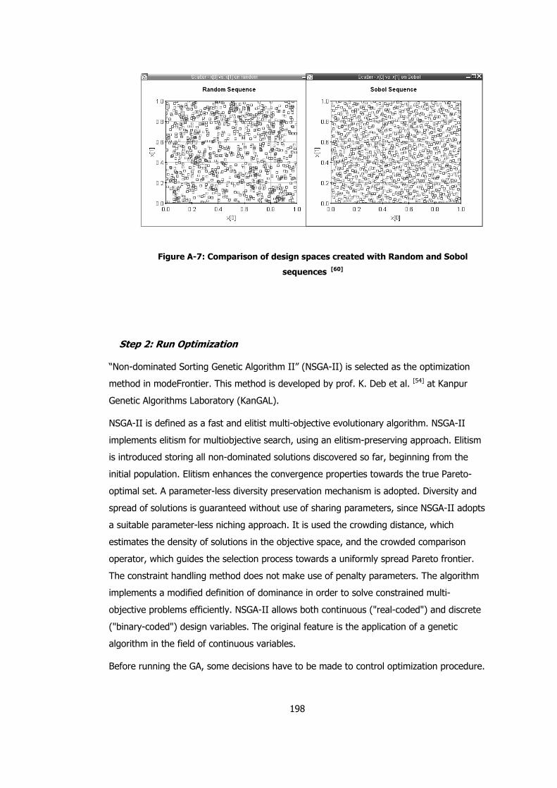
198

Figure A-7: Comparison of design spaces created with Random and Sobol

sequences [60]

Step 2: Run Optimization

“Non-dominated Sorting Genetic Algorithm II” (NSGA-II) is selected as the optimization

method in modeFrontier. This method is developed by prof. K. Deb et al. [54] at Kanpur

Genetic Algorithms Laboratory (KanGAL).

NSGA-II is defined as a fast and elitist multi-objective evolutionary algorithm. NSGA-II

implements elitism for multiobjective search, using an elitism-preserving approach. Elitism

is introduced storing all non-dominated solutions discovered so far, beginning from the

initial population. Elitism enhances the convergence properties towards the true Pareto-

optimal set. A parameter-less diversity preservation mechanism is adopted. Diversity and

spread of solutions is guaranteed without use of sharing parameters, since NSGA-II adopts

a suitable parameter-less niching approach. It is used the crowding distance, which

estimates the density of solutions in the objective space, and the crowded comparison

operator, which guides the selection process towards a uniformly spread Pareto frontier.

The constraint handling method does not make use of penalty parameters. The algorithm

implements a modified definition of dominance in order to solve constrained multi-

objective problems efficiently. NSGA-II allows both continuous ("real-coded") and discrete

("binary-coded") design variables. The original feature is the application of a genetic

algorithm in the field of continuous variables.

Before running the GA, some decisions have to be made to control optimization procedure.

199

Figure A.8: Parameters to be set for Genetic Algoritm

Definitions of control parameters presented in Figure A.8 are as follows:

• Number of Generations: This value defines the maximum size of the run. It is

set as 2000 in this work.

• Crossover Probability: This parameter specifies the occurrence probability of

the Classical Cross-Over operator. The value range is 0-1. It is set as 0.9 which

recommended by the program also.

The size of the initial population is usually related to the number of design variables. In

most cases a good initial guess is to set the population size at 3-5 times larger than the

number of design variables [51]. If the chosen population size chosen is too small, there will

not be enough variety among the members of the population. This can lead to a

premature convergence to some local minimum.

Alternatively, if the population size is too large, then it will take a lot more computational

time to evaluate all the members of the population without significantly reducing the

number of generations needed to reach the optimal solution. In the case of a surface PM

motor design there are 9 independent variables as presented in Section 5.1.4. An initial

population size of 50 seems (more than 5 times of independent variables) to be

reasonable.

The maximum generations is limited as 2000 so that after 2000 iterations resulting in

100.000 designs, no more iteration will be performed to avoid excessive work. It is

assumed that before 2000 generations, GE will result an optimized solution which can be

no more improved. Certainly the iteration process can be continued in case of no optimum

solution in 2000 generations.

200

Step 3: Select best solution from optimization pareto set

As for any optimized design problem, several alternative designs may be reached, which

satisfy the defined constraints and requirements. The designs which fit into requirements

are called feasible designs. However, optimum design is best among these feasible designs

in some sense. This could be a minimum weight, size, cost, maximum efficiency, or a

combination of them.

201

A.5 Magnet Data

Remanence Br

Coercive Force Hcb

Intrinsic Coercive force Hci

Max Energy Product

(BH) max

Square Degrees Hk/Hcj

Highest Work temperature

KG T KOe KA/m KOe KA/m MGOe KJ/m Block Cylinder

1 N-35 11.4-11.8

1.18-1.28 ≥10.8 ≥836 ≥12 ≥955 33-36 263-287 >=90% >=86.8% 80

2 N-38 11.8-12.3

1.18-1.28 ≥10.8 ≥860 ≥12 ≥955 36-39 287-310 >=90% >=86.8% 80

3 N-40 12.7-12.9

1.27-1.29 ≥11.0 ≥876 ≥12 ≥955 38-41 303-326 >=90% >=86.8% 80

4 N-42 12.9-13.3

1.29-1.33 ≥10.5 ≥836 ≥12 ≥955 40-43 318-342 >=90% >=86.8% 80

5 N-45 13.3-13.8

1.33-1.38 ≥9.5 ≥756 ≥12 ≥955 43-46 342-366 >=90% >=86.8% 80

6 N-48 13.8-14.2

1.38-1.42

≥ 10.5

≥ 835

≥ 12

≥ 955

46-49 366-390 >=90% >=86.8% 80

7 N-50 13.8-14.5

1.38-1.45

≥ 10.5

≥ 835

≥ 11

≥ 955

47-51 374-406 >=90% >=86.8% 80

8 N-52 14.3-14.8

1.43-1.48

≥ 10.8

≥ 860

≥ 11

≥ 876

50-53 398-422 >=90% >=86.8% 80

9 33M 11.4-11.8

1.14-1.18 ≥10.3 ≥820 ≥14 ≥1114 31-33 247-263 >=90% >=86.8% 100

10 35M 11.8-12.3

1.18-1.23 ≥10.8 ≥860 ≥14 ≥1114 33-36 263-287 >=90% >=86.8% 100

11 38M 12.3-12.7

1.23-1.27 ≥11.0 ≥876 ≥14 ≥1114 38-41 303-326 >=90% >=86.8% 100

12 40M 12.7-12.9

1.27-1.29 ≥11.4 ≥907 ≥14 ≥1114 38-41 303-326 >=90% >=86.8% 100

13 42M 12.8-13.2

1.28-1.32

≥ 11.6

≥ 923

≥ 14

≥ 1114

40-43 318-342 >=90% >=86.8% 100

14 45M 13.2-13.8

1.32-1.38

≥ 11.8

≥ 939

≥ 14

≥ 1114

43-46 342-366 >=90% >=86.8% 100

15 48M 13.6-14.0

1.36-1.40

≥ 11.8

≥ 939

≥ 14

≥ 1114

46-49 366-390 >=90% >=86.8% 100

16 50M 14.0-14.5

1.40-1.45

≥ 13.0

≥ 1033

≥ 14

≥ 1114

48-51 382-406 >=90% >=86.8% 100

17 30H 10.8-11.4

1.08-1.14 ≥10.2 ≥812 ≥17 ≥1353 28-31 223-247 >=90% >=86.8% 120

18 33H 11.4-11.8

1.14-1.18 ≥10.6 ≥844 ≥17 ≥1353 31-33 247-263 >=90% >=86.8% 120

19 35H 11.8-12.3

1.18-1.28 ≥11.0 ≥876 ≥17 ≥1353 33-36 263-287 >=90% >=86.8% 120

20 38H 12.3-12.7

1.23-1.27 ≥11.2 ≥890 ≥17 ≥1353 36-39 287-310 >=90% >=86.8% 120

21 40H 12.7-12.9

1.27-1.29 ≥11.5 ≥915 ≥17 ≥1353 38-41 303-326 >=90% >=86.8% 120

22 42H 12.8-13.2

1.28-1.32

≥ 12.0

≥ 955

≥ 17

≥ 1353

40-43 318-342 >=90% >=86.8% 120

23 45H 13.2-13.5

1.32-1.38

≥ 12.0

≥ 955

≥ 17

≥ 1353

42-46 335-366 >=90% >=86.8% 120

24 46H 13.3-13.8

1.33-1.38

≥ 12.2

≥ 972

≥ 16

≥ 1274

44-47 350-374 >=90% >=86.8% 120

25 48H 13.6-14.3

1.36-1.43

≥ 12.5

≥ 995

≥ 16

≥ 1274

46-49 366-390 >=90% >=86.8% 120

26 30SH 10.8-11.4 1.081.14 ≥10.0 ≥796 ≥20 ≥1672 28-31 223-247 >=90% >=86.8% 150

27 33SH 11.4-11.8

1.14-1.18 ≥10.5 ≥836 ≥20 ≥1672 31-34 247-276 >=90% >=86.8% 150

28 35SH 11.8-12.3

1.18-1.23 ≥11.0 ≥876 ≥20 ≥1672 33-36 263-287 >=90% >=86.8% 150

29 38SH 12.3-12.7

1.23-1.27 ≥11.4 ≥907 ≥20 ≥1972 36-39 287-310 >=90% >=86.8% 150

30 40SH 12.5-12.8

1.25-1.28

≥ 11.8

≥ 939

≥ 20

≥ 1972

38-41 302-326 >=90% >=86.8% 150

31 42SH 12.8-13.2

1.28-1.32 ≥ ≥ ≥ ≥ 40-43 320-343 >=90% >=86.8% 150

202

11.8 939 20 1672

32 45SH 13.2-13.8

1.32-1.38

≥ 12.6

≥ 1003

≥ 20

≥ 1592

43-46 342-366 >=90% >=86.8% 150

33 30UH 10.8-11.4

1.08-1.14 ≥10.2 ≥812 ≥25 ≥1990 28-31 223-247 >=90% >=86.8% 180

34 33UH 11.3-11.7

1.13-1.17

≥ 10.7

≥ 852

≥ 25

≥ 1990

31-33 247-263 >=90% >=86.8% 180

35 35UH 11.7-12.1

1.17-1.21

≥ 10.7

≥ 852

≥ 25

≥ 1990

33-36 263-287 >=90% >=86.8% 180

36 38UH 12.1-12.5

1.21-1.25

≥ 11.4

≥ 907

≥ 25

≥ 1990

36-39 287-310 >=90% >=86.8% 180

37 40UH 12.5-12.8

1.25-1.28 ≥11.4

≥ 907

≥ 25

≥ 1990

38-41 302-326 >=90% >=86.8% 180

38 28EH 10.5-10.8

1.05-1.08 ≥9.5 ≥756 ≥30 ≥2388 26-29 207-231 >=90% >=86.8% 200

39 30EH 10.8-11.4

1.08-1.14 ≥9.5 ≥756 ≥30 ≥2388 28-31 223-241 >=90% >=86.8% 200

40 33EH 11.3-11.7

1.13-1.17

≥ 10.2

≥ 812

≥30 ≥2388 31-33 247-263 >=90% >=86.8% 200

41 35EH 11.7-12.1

1.17-1.21

≥ 10.2

≥ 812

≥30 ≥2388 33-36 263-287 >=90% >=86.8% 200

42 38EH 12.1-12.5

1.21-1.25

≥ 11.4

≥ 907

≥30 ≥2388 36-39 287-310 >=90% >=86.8% 200

43 30AH 10.8-11.3

1.08-1.13

≥ 10.2

≥ 812

≥ 35

≥ 2785

28-32 223-255 >=90% >=86.8% 220

44 33AH 11.2-11.7

1.12-1.17

≥ 10.2

≥ 812

≥ 35

≥ 2785

31-34 247-271 >=90% >=86.8% 220

Notes: 1. The above-mentioned data of magnetic parameters and physical properties are given at

room temperature. 2. The maximun service temperature of magnet is changeable due to the ratio length and

diameter and environmental factors. Typical magnetic properties:

α(Br) = -0.12%/ testing temperature range: 20～140

α(HcJ) = -0.60%/ testing temperature range : 20～140（Not include Tseries、L-Tseries） µrec =1.05

Tc: N series 312 M series 320 H series 330 SH series 340 UH、EH series 380

T series

α(Br) = -0.11%/ testing temperature range 20～150

α(HcJ) = -0.65～-0.50%/ testing temperature range 20～150

L-······T series (Low Co-efficient of Temperature)

α(Br) （absolute value）＜-0.10%/ testing temperature range 20～180

α(HcJ) （absolute value）＜ -0.50%/ testing temperature range 20～180

PS: 1T=10kGs 1kOe=79.6kA/m 1MGOe=7.96kJ/m3 1mT=10Gs PS: 1T=10kGs 1kOe=79.6kA/m 1MGOe=7.96kJ/m3 1mT=10Gs

203

A.6 Winding Scheme

Figure A.9: Winding scheme of sample motor and new designs

MEASUREMENT OF BRUSHLESS DC MOTOR CHARACTERISTICS...

Documents

Transcript of MEASUREMENT OF BRUSHLESS DC MOTOR CHARACTERISTICS...