Measurement Error in the Schaefer Production Model

Christopher Burns

University of Massachusetts-Amherst

cbburns@acad.umass.edu

Selected Paper prepared for presentation at the Agricultural & Applied Economics

Association’s 2014 AAEA Annual Meeting, Minneapolis, MN, July 27-29, 2014.

Copyright 2014 by Christopher Burns. All rights reserved. Readers may make verbatim copies of

this document for non-commercial purposes by any means, provided that this copyright notice

appears on all such copies.

Measurement Error in the Schaefer Production

Model

Christopher Burns

Abstract

This paper contributes to the existing literature on the Schaefer Production Model by ap-

plying a relatively new method for reducing the bias induced by measurement error, known

as Simulation Extrapolation (SIMEX). We test this new method on logbook data from the Mid-

Atlantic surfclam fishery from 2001-2009. We show that the SIMEX estimator reduces bias in

the parameter estimates for the biological parameters and biomass estimates. This contribution

is important because fishery managers may only have logbook catch and effort data on a few

time periods, which could lead to poor biomass estimates, and potentially leading to a state of

overfishing.

Key words: commercial fisheries, measurement error

1 Introduction

Since the reauthorization of the Magnuson-Stevens Fishery Conservation Act in 2007 (M.S. Act),

fishery managers have been given high standards to meet when determining future management

plans. National Standards One and Two state that management plans must prevent overfish-

ing while achieving the optimum yield for the fishery, and that new management measures be

based on the best scientific information available (U.S. Department of Commerce, 2007). In order

to achieve the objectives outlined in the M.S. Act, fishery managers must know what constitutes

overfishing. This requires information on the biological parameters of fishery. Because biological

data are often not available, fishery managers must make use of catch and effort data to make

inference about the status of the biomass (stock). The most commonly used model is the Schaefer

production model (Schaefer, 1954). This paper1 extends recent work on the Schaefer Production

model (Zhang and Smith, 2011), attempting to deal with the estimation issues, such as measure-

ment error, by using a Monte Carlo method known as SIMEX.1Special Thanks to Dan Lass, Sylvia Brandt and John Staudenmayer for their advice and support.

1

The Schaefer Production model is a bioeconomic model that links an economic model of pro-

duction to a biological growth model for a fishery. The advantage to this model is that fishery

managers can use logbook data obtained from active vessels in the fishery to estimate the biolog-

ical parameters. The Schaefer production model is estimated as a two-stage model. In the first

stage production function, harvest is modeled as a function of effort and the biomass. Typically

a Cobb-Douglas functional form is assumed, though more recent work has looked at more flexi-

ble functional forms (Zhang and Smith, 2011). This first stage model cannot be directly estimated

with the available data, since biomass is not observed. Instead a proxy variable, such as catch-

per-unit effort (CPUE), is used in its place. This proxy variable is then substituted into the second

stage growth model, and biological parameters for the fishery can be estimated. The problem

with this method is that using the CPUE proxy contains measurement error, leading to inconsis-

tent estimates of biological parameters in the second stage of the model. This paper examines

how to mitigate the impact of measurement error, so that fishery managers can have more precise

estimates of biological parameters.

Previous work on this model has highligted important considerations in the methods used to

obtain the biological parameters. Punt (1992) shows that when estimating the biomass using catch

and effort data, the method used to fit the model is much more important than the actual paramet-

ric form. Polacheck et al. (1993) note that there are three models which are widely used for fitting

a dynamic biomass to observed data; the effort-averaging estimation method (Gulland, 1961; Fox,

1975), process-error estimators (Walters and Hilborn, 1976; Schnute, 1977) and observation-error

estimators (Pella and Tomlinson, 1969; Butterworth and Andrew, 1984). Observation error estima-

tors refer to appending error in the first stage production model, while process-error estimators re-

fer to appending error to the second stage growth model. The effort-averaging estimation method

refers to averaging effort from the vessel data. Each of these methods has potential drawbacks.

Polacheck et al. (1993) examine each of these estimators, concluding that the effort-averaging es-

timator is biased and process-error estimators have high variability. They further conclude that

the observation error method should provide the most precise parameter estimates, but that any

method should be assessed with a Monte Carlo study before implementation.

More recently, Zhang and Smith (2011) proposed a more generalized production function, and

use panel-data methods to obtain a consistent estimator for biological parameters. They note three

2

empirical problems with estimating the classic Schaefer model; 1) the biological dynamics have

natural variation or process error; 2) the production function has stochastic shocks, which makes

the inferred stock noisy; and 3) the fishing production function, usually Cobb-Douglas, has an

extremely restrictive form. Without taking these three factors into account simultaneously, the

resulting estimation of the classic Schaefer production model will lead to biased and inconsis-

tent parameter estimates. This means that estimates of the growth parameters and the biomass

estimates are not reliable. Given that the growth model is non-linear in the parameters, there is

great potential for biased results. Uhler (1980) showed that parameter estimates from the Schaefer

production model could be biased by up to 40%.

This paper further extends the existing literature on the Schaefer production model by apply-

ing a relatively new method for reducing the bias induced by measurement error. This method,

known as simulation extrapolation (SIMEX), is a Monte Carlo method for reducing bias first de-

veloped by Cook and Stefanski (1994). After estimating a more generalized Schaefer production

model, we apply the SIMEX estimator to the second stage growth model. We show that this

method can further improve the generalized Schaefer model, which can be particularly useful

when a fishery manager has limited data. To test our method we use data from the Mid-Atlantic

surfclam fishery for 2001-2009.

Using logbook data from the Mid-Atlantic surfclam fishery, we estimate three different models;

the classic Schaefer model, the generalized Schaefer Production model and a SIMEX model. In

order to apply the measurement error correction method known as SIMEX, we must also estimate

the measurement error variance. To assess the bias in the estimates of each model, we use data on

the biomass estimates for the Mid-Atlantic surfclam fishery, obtained from the Northeast Fisheries

Science Center (Northeast Fisheries Science Center, 2010). Although the scientific estimates are

known to contain some measurement error, we use these estimates as the truth when evaluating

each model.

This has important policy implications for fishery managers. If fishery managers make de-

cisions about setting the TAC based on biased estimates of the biomass, it can lead to reduced

economic rent for harvesters and possible collapse of the fishery. Additionally, the efficiency gains

from moving to an individual tradable quota fishery (ITQ), such as the Mid-Atlantic surfclam

fishery, depend on correct setting of the TAC. Thus if fishery managers use biased estimates of the

3

biomass, the goals set in the reauthorized M.S. Act will not be met (U.S. Department of Commerce,

2007) and gains in economic efficiency will not be realized.

The rest of the paper will proceed as follows: Section 2 explains the methodology of the classic

Schaefer and generalized Schaefer Production Model. In Section 3 we build a measurement error

model and describe the SIMEX estimator. Section 4 describes the Mid-Atlantic surfclam logbook

data. Section 5 reports results from all three models and compares the biomass estimates to the

scientific estimates. Section 6 summarizes the findings of this paper and discusses future research.

2 Methodology

We begin by describing the two-stage classic Schaefer production model. In the first stage a pro-

duction function is estimated, followed by the second stage estimation of a logistic growth model

for the biomass.

2.1 Classic Schaefer Production Model

The classic Schaefer production model is

Ht = qEtXt (1)

whereXt is the biomass in time t, Ht is harvest in time t, and Et is fishing effort in time t. The state

equation or growth model is

Xt+1 = Xt + rXt(1−Xt

K)−Ht (2)

where the intrinsic growth rate r, carrying capacity K, and catchability coefficient q are the bi-

ological parameters to be estimated. The second stage growth model expresses the biomass in

the next period as the sum of the current period biomass and growth, minus the current period

harvest. If biomass, harvest and effort information are all observed, this model can be estimated

under regularity conditions (Zhang and Smith, 2011). However, the fishery biomass is typically

not observed, and is therefore a latent variable to the econometrician.

To estimate the above model when biomass is unknown a proxy such as catch-per-unit-effort

(CPUE) is often used. Let yt denote CPUE, defined as yt =Ht

Et. From equation 2, CPUE is pro-

4

portional to the unobserved biomass, such that Xt =ytq

. The standard approach to the Schaefer

production model substitutes this proxy into equation 2 and appends an additive error term. The

resulting second stage growth model is

yt+1 = (1 + r)yt −r

qKy2t − qHt + εt (3)

Under exogeneity conditions, E(εt|yt) = 0, this equation can be estimated by ordinary least

squares.

There are several drawbacks to this particular estimator. First, the production function as-

sumes a very restrictive form, with constant returns to scale imposed. Second, the production

function is usually assumed to have an error term that captures variability in the harvest from

random events, such as weather. Thus when yt is substituted in equation 3, the right-hand side of

the equation has yt and y2t , both of which are measured with error. Uhler (1980) points out that if

the stock is measured with significant noise due to the error in the production function, then the

CPUE proxy for stock will lead to biased estimators. Additionally, the functional form of equa-

tion 3 assumes a logistic growth model. Many other functional forms for the growth model could

be fitted to the data, such as exponential or quadratic form.

2.2 Generalized Schaefer Production Model

Following previous work (Burns, 2013) we specify a more flexible Cobb-Douglas production func-

tion in the first stage.

Hit = (Zβ1

it1Zβ2

it2 )qXtexp(bi+εit) (4)

with i = 1, . . . , 70 vessels, t = 1, . . . , 9 time periods, biind.∼ N(0, σ2b ), and εit

i.i.d.∼ N(0, σ2). Let Hit =

total bushels harvested by vessel i in year t, Zit1 = total hours fished by vessel i in year t, and Zit2

= length of vessel i in year t. This functional form does not impose constant returns to scale and

also captures unobserved heterogeneity in the fishing fleet through the random effect term bi.

Taking natural logs we can rewrite equation 4 as linear in the parameters. Let lowercase letters

denote natural log, e.g ln(Xt) = xt, then production function becomes

hit = β1zit1 + β2zit2 + bi + εit + lnq + xt (5)

5

Following (Zhang and Smith, 2011) the unobserved stock in year t can be estimated by a time-

varying fixed effect. We create a series of indicator variables (Dt) and then estimate a stock index

for each year (δt). Let Dt =1 if year t and 0 otherwise. Then equation 5 can be written

hit = β1zit1 + β2zit2 + bi + εit +

9∑t=1

δtDt (6)

From equation 6 the stock index is written as δt = lnq + xt. The stock index can be estimated by

δt = (ht − zt1β1 − zt2β2) + εt (7)

where ht =∑nt

i=1 hitnt

, ztj =∑nt

i=1 zitjnt

for j = 1, 2 and εt =∑nt

i=1 eitnt

. Rearranging the stock index, the

biomass in time period t can be estimated as

Xt =exp(δt)

q(8)

In order to estimate this quantity the catchability coefficient, q, must be estimated by the second-

stage growth model.

∆Yt+1 = Yt+1 − Yt = α1Yt − α2Y2t − α3Ht + εt (9)

where Yt = exp(δt), α1 = r, α2 = rqK and α3 = q. Then exp(δt) = ˆqXt, and stock is estimated as

Xt = exp(δt)q

The measurement error in equation 9 comes from the estimation of Yt+1 , Yt , and Yt2, which are

a function of the estimated stock index, δt. The remaining error in the estimated stock index will

be correlated with the disturbance in the model, which violates an important assumption of the

classical regression model. The consequences are that the estimated biological parameters in the

second-stage growth model will be biased an inconsistent. We propose another way to correct for

this measurement error, using a Monte Carlo method known as Simulation Extrapolation (SIMEX).

6

3 Measurement Error Model

In this section we specify a measurement error model for the estimated stock index, δt. With

variance for δt known, or at least approximately known, it will then be possible to reduce the

bias by implementing SIMEX. The error is assumed to be additive, with the estimated stock index

equal to the true index plus random error. The measurement error for the stock index is specified

as

δt − δt = ut = zt′β − zt

′β + ηt (10)

where ut|zt ∼ N(0, σ2ut). The measurement error model requires E[ut|zt] = 0 but does not require

the error to be independent of the variables conditioned on. The assumption that ut is independent

of zt is a much stronger assumption than required here.

From the measurement error model above, we can write the measurement error variance as

σ2ut = zt′

[ˆCov(β)

nt

]zt +

σ2ηnt

(11)

where ˆCov(β) is the variance-covariance matrix for the estimated parameters in the first stage

production function. Equation 11 defines the measurement error variance for the stock index. The

variance is allowed to vary over time. We note that because of the off-diagonal elements in the

variance-covariance matrix, the measurement error is not independent between years. We also

allow the measurement error variance to be heteroscedastic over the nine years of our observed

data. Given this estimated of the measurement error variance, we can apply SIMEX as a method to

reduce bias in the parameter estimates. Before addressing the SIMEX algorithm, we first describe

the measurement error problem in the second stage growth model in more detail.

3.1 Linear Models with Nonadditive Measurement Error

In this section we discuss the implications of nonadditive error in the estimation of the general-

ized Schaefer Production Model. We start by examining how the second stage growth model is

estimated. This model estimates the biological parameters using the three covariates; Yt = exp(δt),

Yt2

= exp(δt)2, and Ht, where δt is the stock index in time period t and Ht is the harvest or catch in

time period t. δt has approximately known additive measurement error. While the measurement

7

error for ct is additive, the model is estimated by using Yt, Yt2

andHt. Since the first two covariates

are nonlinear function of the mismeasured δt, the second stage growth model parameter estimates

will not be unbiased.

We motivate the measurement error problem by describing the properties of a naive estimator

for the model. Let xt be a (1 x 3) vector containing the true variables [δt δt Ht]. Then let wt be a (1

x 3) vector containing the estimated or mismeasured variables [δt δt Ht], such that

wt = xt + ut (12)

Defining the vector ut as a (1 x 3) vector, ut=[ut ut 0] , then E[ut|x] = 0. However, because xt enter

into the model through a nonlinear function, call it g(xt), this means E[g(wt)] 6= g(xt).

To show how this will impact estimation of the model, we specify the design matrix by stacking

the vector of wt for all nine time periods, t = 1, . . . , 9

W =

Y1 Y1

2H1

......

...

Y9 Y92

H9

(13)

In the traditional setup of the generalized Schaefer production model, the second stage growth

model is specified as linear in the parameters. Under the classical regression model assumptions,

the biological parameters can be estimated using ordinary least squares. Let y be the response

vector of the difference Yt+1 − Yt for t = 1, . . . , 9, such that

y =

y1

...

y9

(14)

The naive growth model can be written

y = Wβ + ε (15)

8

The ordinary least squares estimator for the naive growth model parameters is

β = (W′W)−1(W

′y) (16)

The classical regression model assumptions define this estimator to be unbiased and consistent

when W is not measured with error. Using our naive estimator above, the asymptotic properties

can be evaluated by making a few more assumptions. Following, Greene (2003) let

plim(W

′W

n) = Q∗ + Σu (17)

where Q∗ = plim X′Xn , and Σu is the Variance-Covariance matrix of u, i.e. the measurement error

variance-covariance matrix. The probability limit of β is then

[Q∗ + Σu]−1Q∗β 6= β (18)

Thus, the estimator is not consistent for the true parameters. The result of nonadditive measure-

ment error in the linear model is that the estimates of biomass, which are a function of the biased

parameter estimates, will be biased and inconsistent. In a situation where measurement error is

present, identification of the parameters in the model is often an associated issue. One option is to

bring in outside information to help identify the model (Greene, 2003). We identify the parameter

estimates through the estimated measurement error variance. In the next section we show how

the estimated measurement error variance to reduce bias in the naive estimates using SIMEX.

3.2 SIMEX Parameter Estimates

SIMEX is a two-step simulation-based method of estimating and reducing bias due to measure-

ment error. In the first step, simulated data are obtained by adding additional measurement error

to the data in a resampling-like process. This establishes a trend of measurement error-induced

bias versus the variance of the added measurement error. In the second step, an extrapolation

method fits a trend line back to a point where the measurement error variance is zero. The key un-

derlying SIMEX is the fact that the effect of measurement error on an estimator can be determined

experimentally through simulation (Carroll et al., 2012). It can be shown that under a number of

9

different measurement error specifications that SIMEX provides approximately consistent param-

eter estimates. SIMEX is very general in the sense that the bias due to measurement error in almost

any estimator of almost any parameter can be estimated and corrected, at least approximately.

In the simulation step we generate measurement error with variance (1+λ)σ2ut for the stock in-

dex. The additional measurement error variance λσ2ut, is generated at different values of λ, where

λ = (0, 0.375, 0.75, 1.125, 1.50). Using the simulated data, the growth model is estimated 10,000

times for each value of λ. Finally, at each value of λ, we calculate the mean for each parameter

estimate. Let the mean for each of the k parameter estimates be αk, shown as dots in the figure 1.

Figure 1: An example of the SIMEX Simulation step for α

The extrapolation step fits a model by regressing the estimated αk on λ, and then extrapolating

back to λ = −1. Since the generated measurement error variance is now (1 + λ)σ2ut, at λ = −1 the

measurement error collapses to zero.

The last step of the SIMEX method is the extrapolation step. There are several functional forms

which can be chosen, including the linear, quadratic and rational extrapolant functions. Figure 2

shows an example of both the linear and quadratic extrapolation functional forms. We choose a

quadratic extrapolation function for this model, reporting results for both the naive estimates and

quadratic extrapolation function. It should be noted that the choice of the extrapolation function

will affect the SIMEX estimates.

10

Figure 2: An example of the SIMEX Extrapolation Step for α

3.3 Standard Errors of SIMEX Estimates

To obtain standard errors for the SIMEX parameter estimates we use a two-stage bootstrap. The

two-stage bootstrap is different from a one-stage bootstrap because it generates both a response

from a regression model, and the mismeasured covariates, similar to a parametric bootstrap pro-

cedure. One advantage of the two-stage bootstrap is that it gives an estimate of bias.

Below we describe the steps for the two-stage bootstrap from (Buonaccorsi, 2010). This proce-

dure is used to obtain the standard errors for the estimated parameters in the second stage growth

model. Two of the covariates in the model, Yt and Yt2, are measured with error. In the two-stage

bootstrap we generate these variables in b repeated simulations and denote them, wbt1 and wbt2

respectively. The third covariate is the harvest, denoted xbt3, is assumed not measured with error.

For the bth bootstrap sample, generate [ybt, wbt1, wbt2, xbt3], where

ybt = β1wbt1 + β2wbt2 + β3xbt3 + ebt (19)

and the two mismeasured covariates are

wbt1 = exp(δt1 + ubt) (20)

and

wbt2 = (wbt1)2 (21)

11

where ubt|wbt1, wbt2, xbt3ind.∼ N (0, σ2ut) and ebt

i.i.d.∼ N (0, σ2ε ).

The standard errors reported for the SIMEX estimates are from 10,000 simulations using this

two-step data generating process. Estimates of bias are calculated as

Bias(boot) =

∑Bb=1 βbB

− β (22)

4 Data

The data for the empirical analysis come from the National Marine Fishery Service logbook re-

porting system, which documents every harvesting trip taken by every vessel in the Mid-Atlantic

surfclam fishery in the U.S. EEZ (3-200miles offshore). The logbook data are a panel data set con-

taining approximately 24,000 vessel-trip observations, for years 2001-2009. The trip-level data set

includes variables such as bushels harvested, time fishing, time-at-sea, and vessel characteristics

such as vessel length, gross-tons and horsepower. There are a total of eighty-eight different ves-

sels observed over the nine year period. To simplify the correlation structure within each vessel

and because biomass is observed annually, data are aggregated by vessel-year. The resulting data

are reduced to 70 vessels and 285 vessel-year observations. The biological data on the biomass

comes from the Northeast Fisheries Science Center. Summary statistics for the data are presented

in Table 1.

Obs Mean Std.Dev Min MaxHarvest (bushels) 285 93749 82007.6 864 442496Time Fishing (hours) 285 1209.2 951.9 58 3959.4Fuel (gallons) 285 65896 65979.3 876 388204Length (feet) 70 85.7 18.4 28 162Biomass (1000 metric tons) 9 1037 171.9 750 1294

Table 1: Summary statistics 2001-2009

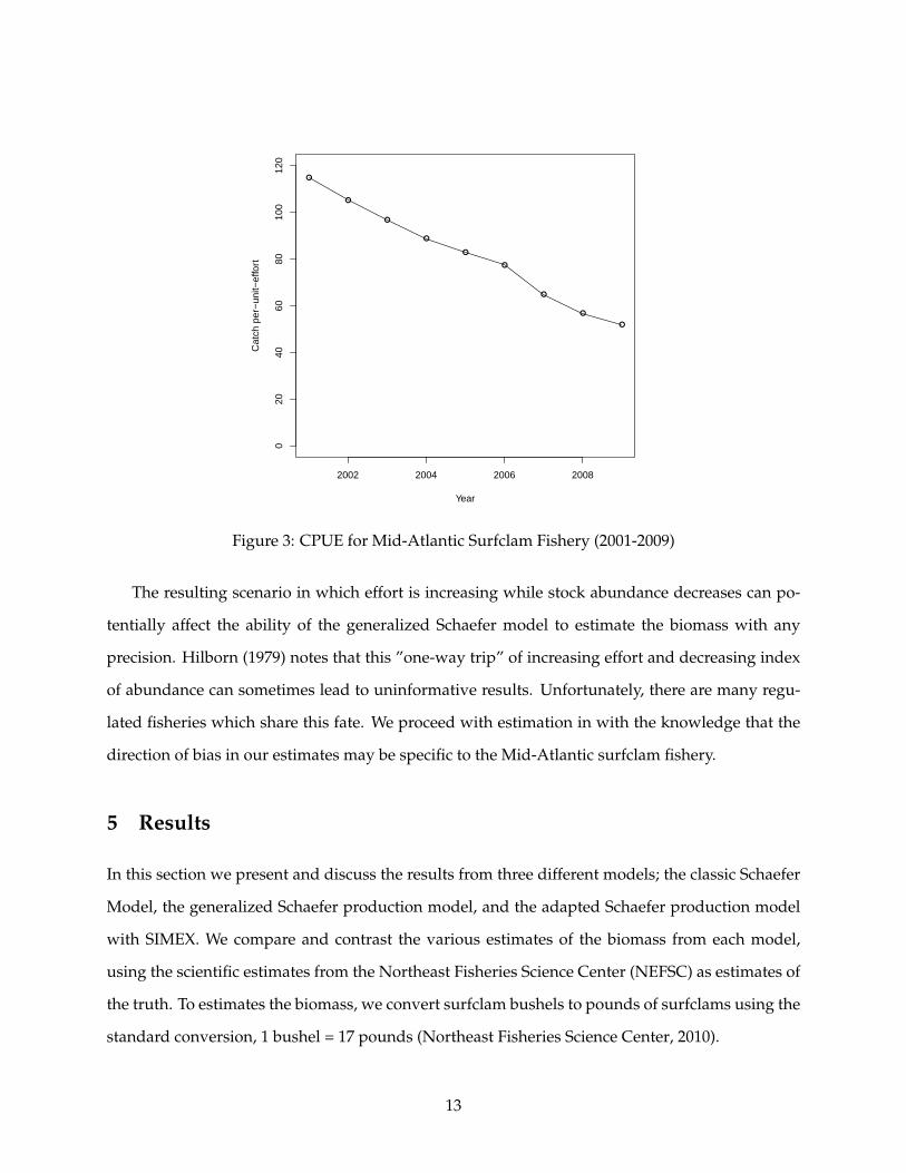
A closer inspection of the data reveals that CPUE has been declining over the nine year time

period, seen in Figure 3. This downward trend reflects declining resource abundance due to re-

peated harvesting from a particular densely populated area of surfclams, located off the northern

New Jersey coast. The result of this fishing behavior means that harvesters are spending more

time-at-sea as the resource is becoming depleted.

12

●

●

●

●

●

●

●

●

●

2002 2004 2006 2008

020

4060

8010

012

0

Year

Cat

ch p

er−

unit−

effo

rt

Figure 3: CPUE for Mid-Atlantic Surfclam Fishery (2001-2009)

The resulting scenario in which effort is increasing while stock abundance decreases can po-

tentially affect the ability of the generalized Schaefer model to estimate the biomass with any

precision. Hilborn (1979) notes that this ”one-way trip” of increasing effort and decreasing index

of abundance can sometimes lead to uninformative results. Unfortunately, there are many regu-

lated fisheries which share this fate. We proceed with estimation in with the knowledge that the

direction of bias in our estimates may be specific to the Mid-Atlantic surfclam fishery.

5 Results

In this section we present and discuss the results from three different models; the classic Schaefer

Model, the generalized Schaefer production model, and the adapted Schaefer production model

with SIMEX. We compare and contrast the various estimates of the biomass from each model,

using the scientific estimates from the Northeast Fisheries Science Center (NEFSC) as estimates of

the truth. To estimates the biomass, we convert surfclam bushels to pounds of surfclams using the

standard conversion, 1 bushel = 17 pounds (Northeast Fisheries Science Center, 2010).

13

5.1 Classic Schaefer Production Model

In table 2 we present estimation results for the second-stage growth model from classic Schaefer

Production Model. This model uses CPUE as a proxy for the stock. In the table below r represents

intrinsic growth rate, K is carrying capacity and q is the catchability coefficient.

Variable Estimater 0.532

(0.379)r/qK -5.4E-04

(0.002)q 2.72E-06

(5.1E-06)

σ2e 7.416*p < 0.1, **p <0.05, ***p<0.01

Table 2: Classic Schaefer Model Estimates for Growth Equation

Using the CPUE estimator, we can estimate the biomass as Xt = ytq . Biomass estimates from

classic Schaefer Production Model (Sch est.) are shown below in Table 3. The NEFSC estimates

of biomass are treated as true measures in the table below. All biomass estimates are reported

in thousands of metric tons. Variance and standard error estimates for the biomass are obtained

using a bootstrap method. Confidence intervals are reported as 95% approximate Wald intervals.

Year NEFSC est. Sch est. 95% lower 95% upper % Bias2001 1294 520 312 728 -60%2002 1207 476 290 662 -61%2003 1128 438 265 611 -61%2004 1104 402 239 565 -64%2005 1079 375 209 541 -65%2006 1013 350 207 493 -65%2007 912 294 177 411 -68%2008 827 257 152 362 -69%2009 750 235 140 330 -69%

Table 3: Classic Schaefer Biomass Estimates (1000MT)

Using the NEFSC estimates as the true value, the average bias for the classic Schaefer Model is

-65%. Clearly the model does a poor job of estimating the biomass for the fishery, with significant

downward bias in each year. Although a fishery manager might not see this as a problem, given

that estimates of maximum sustainable yield (MSY) would be conservative, we cannot be sure this

14

would be the case in another fishery. As Uhler (1980) points out, the biases in the model are too

complex to estimate beforehand, and so a different fishery could certainly have significant bias in

the opposite direction. It is certainly possible this result is limited to the Mid-Atlantic surfclam

fishery. At the very least, these estimates of the biomass are not very informative because they are

biased downward by a substantial amount.

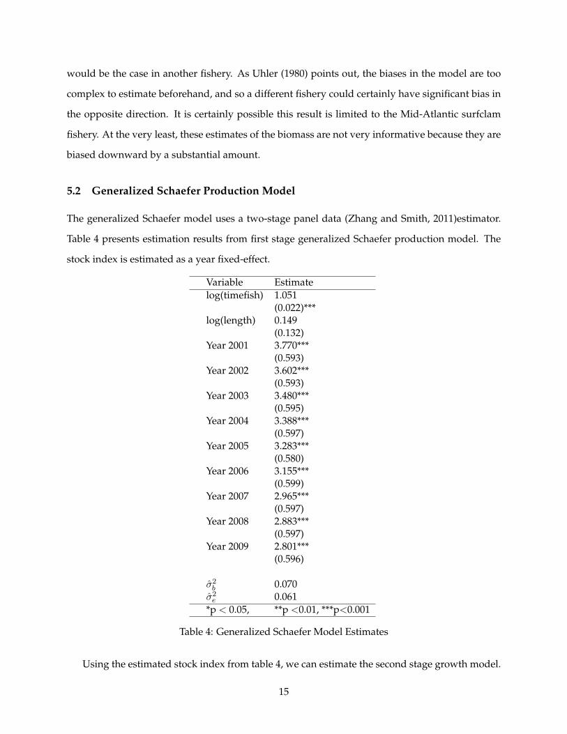
5.2 Generalized Schaefer Production Model

The generalized Schaefer model uses a two-stage panel data (Zhang and Smith, 2011)estimator.

Table 4 presents estimation results from first stage generalized Schaefer production model. The

stock index is estimated as a year fixed-effect.

Variable Estimatelog(timefish) 1.051

(0.022)***log(length) 0.149

(0.132)Year 2001 3.770***

(0.593)Year 2002 3.602***

(0.593)Year 2003 3.480***

(0.595)Year 2004 3.388***

(0.597)Year 2005 3.283***

(0.580)Year 2006 3.155***

(0.599)Year 2007 2.965***

(0.597)Year 2008 2.883***

(0.597)Year 2009 2.801***

(0.596)

σ2b 0.070σ2e 0.061*p < 0.05, **p <0.01, ***p<0.001

Table 4: Generalized Schaefer Model Estimates

Using the estimated stock index from table 4, we can estimate the second stage growth model.

15

Table 5 presents results from second stage estimation of the growth model for the generalized

Schaefer Production Model. Just as in the classic Schaefer Production Model, the parameter esti-

mates are not significant due to a high degree of collinearity among the right-hand side variables.

Variable Estimater 0.181

(0.318)r/qK 1.38E-04

(0.005)q 5.69E-07

(1.46E-06)

σ2e 0.940*p < 0.1, **p <0.05, ***p<0.01

Table 5: Generalized Schaefer Model Estimates for Growth Equation

From table 5, the catchability coefficient q is used to estimate the biomass for the fishery Xt,

where Xt = ytq . Table 6 below shows estimates of biomass using the Generalized Schaefer Model

(Gen. Schaefer). All estimates are reported in thousands of metric tons (1000 MT). Variance esti-

mates for the biomass were obtained using a stratified bootstrap method.

Year NEFSC Gen. Schaefer 95% Lower 95% Upper % Bias2001 1294 996 671 1321 -23 %2002 1207 842 564 1120 -30 %2003 1128 745 504 986 -34 %2004 1104 681 461 901 -38 %2005 1079 612 419 804 -43 %2006 1013 539 366 712 -47 %2007 912 446 300 592 -51 %2008 827 411 278 544 -50 %2009 750 368 242 494 -50 %

Table 6: Generalized Schaefer Model Biomass Estimates (1000MT)

The average bias for the Generalized Schaefer Model is - 41%. While this is much smaller than

the classic Schaefer Production Model, it does consistently underestimate the biomass in each year

except 2001. The 95% confidence intervals for the generalized Schaefer model contain the NEFSC

biomass estimate for 2001 only. If we are to believe that the NEFSC biomass estimates represent an

unbiased picture of the fishery stock, then this would seem to be a significant problem for fishery

managers. A fishery manager using this method with this particular data would likely set the

16

total allowable catch too low or simply not be able to use this model for estimation of the biomass.

The results from table 6 show that the confidence intervals from the generalized Schaefer Model

do not contain the true biomass in any year, a disappointing result.

5.3 Generalized Schaefer Production Model with SIMEX

Table 7 below shows estimates from the second stage growth model using the SIMEX with a linear

extrapolation functional form. All SIMEX estimates are 10,000 simulations at each λ, resulting in a

total of 40,001 simulated datasets. Standard errors reported are from using a two-stage bootstrap

method. It can be seen that none of the parameter estimates are statistically significant, due to

high multicollinearity in the variables. The important difference is the point estimates are different

than the generalized Schaefer Production Model. The difference in the estimate of q is particularly

important because it is used to estimate the biomass. These estimates can be seen in table 8.

Variable Estimater 0.103

(0.620)r/qK 1.36E-03

(0.130)q 2.67E-07

(5.354E-06)

σ2e 0.778*p < 0.1, **p <0.05, ***p<0.01

Table 7: Generalized Schaefer Model with SIMEX, Estimates for Growth Model

The biomass estimates, calculated in thousands of metric tons (1000MT), are shown in table 8.

Variance and standard error estimates of the biomass were obtained using the two-stage bootstrap

method. The average bias for the SIMEX estimates of biomass, using the NEFSC biomass estimates

as truth, is -17%. This is less than half the amount of bias in the generalized Schaefer model

estimates. Additionally, the 95% confidence interval in each year covers the NEFSC estimate.

Note that these intervals are wider than the generalized Schaefer model, because they account for

measurement error.

17

Year NEFSC est. SIMEX est. 95% Lower 95% Upper % Bias2001 1294 1399 937 1861 8 %2002 1207 1183 781 1585 -2%2003 1128 1047 656 1438 -7%2004 1104 956 603 1309 -13%2005 1079 860 549 1171 -20%2006 1013 757 481 1033 -25%2007 912 626 400 852 -31%2008 827 577 378 776 -30%2009 750 531 336 726 -29%

Table 8: SIMEX Biomass Estimates (1000MT)

6 Discussion

This paper explores the impact of measurement error in the Schaefer Production Model and de-

scribes a Monte Carlo method for reducing bias in the parameters. The Schaefer production model

is a two-stage model that estimates the biomass of a fishery using only information on catch and

effort, usually obtained through vessel logbook data. We build on previous work by Zhang and

Smith (2011) to reduce bias in the parameter estimates of a more generalized version of the Schae-

fer Production Model by using a Monte Carlo method called simulation extrapolation (SIMEX).

Using data from the Mid-Atlantic surfclam fishery from 2001-2009, along with scientific esti-

mates of the biomass from NEFSC, we show that the remaining measurement error in a general-

ized Schaefer model can still contribute to significant bias in the estimates of biomass, up to -41%

in this case. A fishery manager using this method would not have much reason to be confident

in setting a total allowable catch with such bias. Obtaining unbiased estimates of the biomass is

crucial to effective fishery management. A total allowable catch that is set too high could put a

fishery on a trajectory towards collapse, while a total allowable catch that is set too low can lead

to economic loss of rents. We show that fishery managers can obtain more truthful estimates of

the biomass after correcting for the measurement error with SIMEX. The results show that the bias

in the biological parameters, and biomass estimates, is dramatically less than either the classic

Schaefer model or the generalized Schaefer model.

The generalized Schaefer production model attempts to simultaneously deal with three prob-

lems inherent in the Schaefer production model, including; 1) the error in the production function,

2) the error in the second stage growth model, and 3) restrictive functional form in the production

18

function. The idea behind the generalized Schaefer production model is that a stock index can be

created using a fixed effects estimator for the production function. We further reduce bias using

the SIMEX algorithm. The average remaining bias in the SIMEX estimates is -17%. This is less than

half the average bias in the generalized Schaefer production model, at -41%. Additionally, all 95%

confidence intervals from the SIMEX estimates cover the NEFSC estimate. Only one confidence

interval from the generalized Schaefer production model covers the NEFSC estimate, while none

of the intervals cover the truth using the classic Schaefer production model.

While these findings would suggest this additional measurement error correction method im-

proves on previous models, it should be noted that these findings may only apply to the Mid-

Atlantic surfclam fishery. Because the surfclam is a slow-growing mollusk, the dynamics of the

growth model may be very different from a pelagic fishery. We intend to apply this method in

several different kinds of fisheries, including pelagic and other fisheries with significantly more

variation in the biomass, before making any definitive conclusions about the model. We think this

model is a good first step towards giving fishery managers a more reliable estimate of the biomass

when they only have catch and effort data obtained through vessel logbooks.

19

References

Buonaccorsi, J. (2010). Measurement error : models, methods, and applications. Boca Raton: CRC Press.

Burns, C. (2013). Correcting for measurement error in a stochastic frontier model: A fishery con-

text. In 2013 Annual Meeting, August 4-6, 2013, Washington, DC, Number 150499. Agricultural

and Applied Economics Association.

Butterworth, D. and P. Andrew (1984). Dynamic catch-effort models for the hake stocks in icseaf

divisions 1.3-2.2. Coli. Scient. Pap. Int. Comm. SE Atl. Fish 11, 29–58.

Carroll, R. J., D. Ruppert, L. A. Stefanski, and C. M. Crainiceanu (2012). Measurement error in

nonlinear models: a modern perspective. CRC press.

Cook, J. R. and L. A. Stefanski (1994, December). Simulation-Extrapolation Estimation in Paramet-

ric Measurement Error Models. Journal of the American Statistical Association 89(428), 1314–1328.

Fox, W. W. (1975). Fitting the generalized stock production model by least-squares and equilibrium

approximation. Fish. Bull 73(1), 23–37.

Greene, W. H. (2003). Econometric Analysis, Volume 97. Prentice Hall.

Gulland, J. A. (1961). Fishing and the stocks of fish at iceland. Fishery investigations. Ser. 2 23(4).

Hilborn, R. (1979). Comparison of fisheries control systems that utilize catch and effort data.

Journal of the Fisheries Board of Canada 36(12), 1477–1489.

McCulloch, C. E. and S. R. Searle (2000, December). Generalized, Linear, and Mixed Models. Wiley

Series in Probability and Statistics. Hoboken, NJ, USA: John Wiley & Sons, Inc.

Northeast Fisheries Science Center, N. (2010). 49th Northeast Regional Stock Assessment Work-

shop 49th Northeast Regional Stock Assessment Workshop ( 49th SAW ). Technical Report

February.

Pella, J. J. and P. K. Tomlinson (1969). A generalized stock production model. Inter-American Tropical

Tuna Commission.

20

Pinheiro, J., D. Bates, S. DebRoy, D. Sarkar, and R Core Team (2013). nlme: Linear and Nonlinear

Mixed Effects Models. R package version 3.1-111.

Polacheck, T., R. Hilborn, and A. E. Punt (1993). Fitting surplus production models: comparing

methods and measuring uncertainty. Canadian Journal of Fisheries and Aquatic Sciences 50(12),

2597–2607.

Punt, A. (1992). Selecting management methodologies for marine resources, with an illustration

for southern african hake. South African Journal of Marine Science 12(1), 943–958.

R Core Team (2013). R: A Language and Environment for Statistical Computing. Vienna, Austria: R

Foundation for Statistical Computing.

Schaefer, M. B. (1954). Some aspects of the dynamics of populations important to the management of the

commercial marine fisheries. Inter-American Tropical Tuna Commission.

Schnute, J. (1977). Improved estimates from the schaefer production model: theoretical consider-

ations. Journal of the Fisheries Board of Canada 34(5), 583–603.

Uhler, R. S. (1980, August). Least Squares Regression Estimates of the Schaefer Production Model:

Some Monte Carlo Simulation Results. Canadian Journal of Fisheries and Aquatic Sciences 37(8),

1284–1294.

U.S. Department of Commerce, M.-S. F. (2007). Management reauthorization act of 2006. US Public

Law 109 479.

Walters, C. J. and R. Hilborn (1976). Adaptive control of fishing systems. Journal of the Fisheries

Board of Canada 33(1), 145–159.

Zhang, J. and M. D. Smith (2011, May). Estimation of a Generalized Fishery Model: A Two-Stage

Approach. Review of Economics and Statistics 93(2), 690–699.

21