Measurement and Verification for Demand Response

February, 2013

Measurement and Verification for Demand Response Prepared for the National Forum on the National Action Plan on Demand Response: Measurement and Verification Working Group

AUTHORS:

Miriam L. Goldberg & G. Kennedy Agnew—DNV KEMA Energy and Sustainability

National Forum of the National Action Plan on Demand Response Measurement and Verification for Demand Response was developed to fulfill part of the Implementation Proposal for The National Action Plan on Demand Response, a report to Congress jointly issued by the U.S. Department of Energy (DOE) and the Federal Energy Regulatory Commission (FERC) in June 2011. Part of that implementation proposal called for a “National Forum” on demand response to be conducted by DOE and FERC.

Given that demand response has matured, DOE and FERC decided that a "virtual" project that convened technical experts and stakeholders to work together over a short, defined period to summarize what is currently known and what remaining work is needed for demand response to deliver its benefits would be more useful than an in-person “DR National Forum” conference. Working groups were formed in the following four areas:

1. Framework for evaluating the cost-effectiveness of demand response;

2. Measurement and verification for demand response resources;

3. Program design and implementation of demand response programs; and,

4. Assessment of analytical tools and methods for demand response.

Each working group has published a final report that summarizes its view of what remains to be done in their subject area. This document is one of those four reports.

The Implementation Proposal, and the National Forum with its four working groups’ reports, is part of a larger effort called the National Action Plan for Demand Response. The National Action Plan was issued by FERC in 2010 pursuant to section 529 of the Energy Independence and Security Act of 2007. The National Action Plan is an action plan for implementation, with roles for the private and public sectors, at the state, regional and local levels, and is designed to meet three objectives:

1) Identify requirements for technical assistance to States to allow them to maximize

the amount of demand response resources that can be developed and deployed; 2) Design and identify requirements for implementation of a national

communications program that includes broad-based customer education and support; and

3) Develop or identify analytical tools, information, model regulatory provisions, model contracts, and other support materials for use by customers, states, utilities, and demand response providers.

The content of this report does not imply an endorsement by the individuals or organizations that are participating in NAPDR Working Groups, or reflect the views, policies, or otherwise of the U.S. Federal government.

Measurement and Verification for Demand Response was produced by Miriam L. Goldberg (Measurement and Verification Working Group chair) and Kennedy Agnew of DNV KEMA Energy and Sustainability, for the Lawrence Berkeley National Laboratory, who is managing this work under a contract to the U.S. Department of Energy Office of Electricity Delivery and Energy Reliability under Contract No. DE-AC02-05CH11231.

FOR MORE INFORMATION

Regarding Measurement and Verification for Demand Response, please contact:

Miriam L. Goldberg Charles Goldman DNV KEMA Energy and Sustainability Lawrence Berkeley National Laboratory E-mail: [email protected] E-mail: [email protected]

Regarding the National Action Plan on Demand Response, visit:

http://www.ferc.gov/legal/staff-reports/06-17-10-demand-response.pdf

Regarding the Implementation Proposal for the National Action Plan for Demand Response, visit:

http://www.ferc.gov/industries/electric/indus-act/demand-response/dr-potential.asp

OR

http://energy.gov/sites/prod/files/oeprod/DocumentsandMedia/ImplementationProposalforNAPDRFinal.pdf

Regarding the National Forum for the National Action Plan for Demand Response project, visit:

http://energy.gov/oe/national-forum-demand-response-what-remains-be-done-achieve-its-potential

or please contact:

Lawrence Mansueti David Kathan U.S. Department of Energy U.S. Department of Energy E-mail: [email protected] E-mail: [email protected]

http://www.ferc.gov/legal/staff-reports/06-17-10-demand-response.pdf�

http://www.ferc.gov/industries/electric/indus-act/demand-response/dr-potential.asp�

http://energy.gov/sites/prod/files/oeprod/DocumentsandMedia/ImplementationProposalforNAPDRFinal.pdf�

http://energy.gov/sites/prod/files/oeprod/DocumentsandMedia/ImplementationProposalforNAPDRFinal.pdf�

http://energy.gov/oe/national-forum-demand-response-what-remains-be-done-achieve-its-potential�

mailto:[email protected]�

mailto:[email protected]�

i

Measurem

ent and Verification for D

emand Response

Table of Contents Executive Summary ..................................................................................... vi

Background ................................................................................................................. vi

The Role of M&V for Demand Response as a Resource ....................................... viii

NAESB’s DR M&V Terminology and Common Demand Response Program Concepts ...................................................................................................................... xi

Guidance on M&V Methods for Settlement .......................................................... xiii

Guidance on Impact Estimation ............................................................................... xx

1. Introduction ............................................................................................. 1

1.1. Purpose of This Document ................................................................................ 1

1.2. Report organization ........................................................................................... 3

2. The Role of M&V for Demand Response as a Resource ..................... 4

2.10. Demand response as a resource ........................................................................ 4

2.11. Measuring Demand Response ........................................................................... 5

2.12. Applications for M&V ........................................................................................ 5

2.13. Understanding and Managing Estimation Error for DR ............................... 11

3. NAESB Business Practice Standards .................................................... 16

3.1. Overview ............................................................................................................ 16

3.2. Key Terminology ............................................................................................... 17

3.3. Applications of NAESB Performance Evaluation Methodologies ................ 22

3.4. Applying the NAESB M&V Terminology to Common Demand Response Program Concepts ..................................................................................................... 27

4. M&V Methods for Settlement ............................................................. 32

4.1. Fundamental Method Design Concepts ......................................................... 32

ii

Measurem


emand Response

4.2. Load Characteristics That Affect DR M&V Choices and Accuracy ............... 34

4.3. Program Design Features Affecting M&V Choice and Accuracy ................. 41

4.4. Settlement Issues and Approaches for Particular Program Types .............. 48

4.5. Means to Assess Settlement M&V Accuracy ................................................. 54

5. Impact Estimation .................................................................................. 56

5.1. Impact Estimation Purposes and Contexts .................................................... 56

5.2. Impact Estimation Methods ............................................................................ 60

5.3. Guidance summary ........................................................................................... 70

5.4. Outstanding issues for impact estimation ..................................................... 72

Appendix A. Prior work on DR M&V Methods ....................................... 74

Baseline Methods Assessment Studies.................................................................... 74

Protocols for EE Program Evaluation ...................................................................... 84

Protocols for DR program evaluation ..................................................................... 85

Appendix B. Examples of Existing Baseline Methods for Settlement.. 89

iii

Measurem


emand Response

LIST OF FIGURES Figure ES-1. DR M&V Methods and Results Affect and are Affected by Many Aspects of Program Planning, Design and Operations ........................................................................................ xiii

Figure 3-1. NAESB Demand Response Event Terms ......................................................................... 19

Figure 3-2. Illustration of a Maximum Base Load Performance Evaluation Methodology 26

Figure 4-1. DR M&V Methods and Results Affect and are Affected by Many Aspects of Program Planning, Design, and Operations ........................................................................................ 33

LIST OF TABLES

Table ES-1. M&V Needs for Common DR Contexts ........................................................................ viii

Table ES-2. Summary of Common DR Mechanisms and NAESB DR M&V Methods ............. xi

Table ES-3. Recommended Baseline Adjustments by Notification Timing and Load Characteristics ..................................................................................................................................................xv

Table ES-4. Summary of Impact Estimation Applications ...............................................................xxi

Table ES-5. Typical Usefulness of DR Impact Estimation Methods by End-use Participant Type and Perspective .................................................................................................................................. xxii

Table 2-1. M&V Needs for Common DR Contexts .............................................................................. 8

Table 3-1. NAESB Service Types and Applicable Performance Evaluation Methodologies 20

Table 3-2. NAESB Criteria for Performance Evaluation Methodologies .................................... 20

Table 3-3. Summary of Common Demand Response Program Mechanisms ......................... 28

Table 4-1. Recommended Baseline Adjustments by Notification Timing and Load Characteristics ................................................................................................................................................. 46

Table 5-1. Typical Usefulness of DR Impact Estimation Methods by End-Use Participant Type and Perspective .................................................................................................................................... 59

Table 5-2. Typical Usefulness of DR Impact Estimation Methods by End-Use Participant Type and Perspective .................................................................................................................................... 70

Table B-1. Examples of Customer Baseline Methodologies ........................................................... 90

iv

Measurem


emand Response

Table B-2 Examples of Baseline Adjustments .................................................................................... 93

v

Measurem


emand Response

Acknowledgements Measurement and Verification for Demand Response is a product of the National Action Plan on Demand Response Measurement and Verification Working Group.

The authors received guidance and input from the Measurement and Verification Working Group which comprises the following individual members:

Measurement and Verification Working Group Mike Alexander

Ken Corum

Theresa Flaim

Stephen George

Paula Ham-Su

Cheryl A. Hindes

Pacific Gas & Electric

Northwest Power and Conservation Council

Energy Resource Economics

Freeman, Sullivan & Co.

DNV KEMA

Baltimore Gas and Electric Company

David Hungerford

Mark S. Martinez

Julie Michals

Donna Pratt

Nik Schruder

Elizabeth Titus

Craig Williamson

Henry Yoshimura

Elizabeth Stuart, Coordinator

California Energy Commission

Southern California Edison

NEEP

NYISO

Ontario Power Authority

NEEP

EnerNOC Utilities Solutions

ISO New England

Lawrence Berkeley National Laboratory

vi

Measurem


emand Response

Executive Summary BACKGROUND

Purpose of this document This document provides guidance on methods for measurement and verification (M&V) of demand response (DR) in wholesale and retail markets. The document is intended for use by designers and operators of DR programs and market mechanisms, by regulators, and by participants or potential participants in wholesale and retail DR program offerings.

Measurement and verification for DR means the determination of the demand reduction quantities. This document addresses M&V for DR in 2 broad contexts:

1. Settlement, meaning determination of the demand reductions achieved by individual program or market participants, and of the corresponding financial payments or penalties owed to or from each participant.

2. Impact estimation, meaning determination of program-level demand reduction that has been achieved or is projected to be achieved, used for ongoing program valuation and planning.

Some parties are accustomed to thinking of M&V primarily in the context of settlement, and some primarily in the context of impact estimation. In this document, we recognize the importance of measured reductions in both contexts for effective DR design and operation, and draw linkages between the two.

This work is a product of the National Forum for the National Action Plan on Demand Response (NAPDR) which was developed with a goal of helping states to advance the development and deployment of demand response resources. This work contributes to that goal by helping to establish credible measurement of demand reductions provided by DR resources. This document describes M&V methods that work best in various market and program contexts, as well as identifying the types of inaccuracies to which different methods are subject. In addition to providing guidance on best practices for DR M&V, the document also identifies areas for further work to enhance guidance on DR M&V best practices.

The intent of this document is to provide common language and guidance on best DR M&V practices in various market and program contexts including wholesale capacity or

vii

Measurem


emand Response

energy markets, and DR programs in retail markets, all with varying operating rules. The document generally follows the terminology and framework of the NAESB Business Practices Standards document on Measurement and Verification for DR, and provides additional guidance.

Importance of M&V for Demand Response Providing meaningful M&V for DR performance is important for several reasons including the following:

First, providing accurate payments to active DR resources leads to improved market efficiency at both the wholesale and retail level. For programs that settle with DR participants according to their measured reductions, providing accurate payments in the market depends on accurate and timely measurement of demand response reductions.

Second, the ability to predict DR response at the individual and aggregate level improves operational efficiency for both wholesale and retail markets. Good prediction depends on reliable measurements of DR performance.

Third, measured DR performance is a key input to planning and design of retail programs. Cost-effectiveness assessment in particular depends on this measurement.

Finally, meaningful measurement of DR performance provides the basis for fair and transparent financial flows to and from market participants. Belief in the fairness of the process and transparency of the results is the underpinning of market confidence.

Areas Addressed This work includes:

• A framing discussion of demand response as a resource, with an overview of the role of M&V, also referred to as performance evaluation.

• A review of the NAESB Business Practice Standards for DR M&V. These Business Practice Standards are directed to the determination of achieved DR demand reduction quantities, and provide some basic terminology for describing M&V methods.

• Guidance on M&V methods for settlement, including design considerations and continuing challenges.

• Guidance on impact estimation methods.

viii

Measurem


emand Response

THE ROLE OF M&V FOR DEMAND RESPONSE AS A RESOURCE

How M&V is Used in DR Operations and Planning M&V is used for multiple purposes in the context of Demand Response:

Establishing the eligibility or capability of resources;

Retail settlement;

Wholesale settlement;

Projecting the future performance of an individual resource based on its past performance relative to its capability

Impact estimation of a program or product as a whole;

Forecasting and Planning.

Different methods may be used for each of these purposes. Across these applications, the M&V methodology and its accuracy affect incentives and payments to participants, costs borne by the market as a whole, program operations, forecasts, and re-design.

The focus of this document is on M&V methods for retail and wholesale settlement, and on program-level impact estimation. DR settlement means determination of the quantity of demand reduction provided by a participant, and of the corresponding financial payments owed. Wholesale settlement is settlement between a market operator and a wholesale DR participant. The wholesale participant may be a DR aggregator or a load-serving entity or distribution company operating a retail program. Retail settlement is settlement between the retail program operator and the retail participants, who may be DR aggregators or individual end users. Table ES-1 summarizes the M&V needs for settlement and for impact estimation, for some common DR contexts. Particular emphasis is placed on wholesale and retail settlement using baseline methods (see highlighted cells).

TABLE ES-1. M&V NEEDS FOR COMMON DR CONTEXTS

Retail Program or Service Structure

Common Applications

M&V Needed for Participant

Settlement with Retail Program

Operator

M&V Needed for Program

Settlement with Wholesale

Market (if retail program is offered as a wholesale

M&V needed for Program-Level Impact Estimation

ix

Measurem


emand Response

resource) 1

Customer or retail DR aggregator is paid per demand reduction amount

Demand Bidding/ Buyback, Peak-Time Rebate

Measured demand reduction for the individual customer or DR aggregator

Measured demand reduction for the aggregate


Customer is paid based on participation metrics

Mass market Direct Load Control

Verification of event participation



Customer pays for usage by time interval

Dynamic or fixed time-varying rates (Block Time-of-Use, Critical Peak Pricing, Variable Peak Pricing, Real Time Pricing)

Metered usage by time interval



Customer pays a penalty/surcharge for usage above a pre-set load level

Contract for differences, firm load demand response, curtailable rates




None—end-use customer participates directly in the wholesale market

Large customer as direct wholesale market participant

N/A Individual measured demand reduction

Individual measured demand reduction

1 This column will not apply to all retail programs; only if the retail program is offered as an aggregate resource in the wholesale market.

x

Measurem


emand Response

End-use customer participates in the wholesale market via a DR Aggregator

End-use customer enrolled by a wholesale DR aggregator and rewarded through agreed sharing of wholesale DR payments

Measured demand reduction for the individual customer



Managing DR M&V Errors There is a fundamental difference between load reduction and generation as resources: It is not possible to meter or otherwise directly observe load reductions. Rather, measurement of the performance of any demand-side resource necessarily means comparing observed load to an estimate of the theoretical load that would have occurred absent the resource’s being dispatched. Any estimate of what the load would have otherwise been is subject to some error. This error should neither be ignored nor exaggerated. Rather, the estimation error can and should be understood and managed.

The means by which the effects of M&V error can be managed and mitigated include the following:

Assessing the magnitude of the systematic and random error;

Operational adjustments based on assessment of errors; and

Program adjustments to reduce M&V errors and mitigate their effects.

This document offers guidance on how to assess, reduce, and mitigate M&V errors through combinations of M&V method specification, program design, and program operations. Before presenting that guidance, we highlight some basic principles and terminology developed by NAESB for DR M&V, and indicate which categories addressed by NAESB are the focus of this work.

xi

Measurem


emand Response

NAESB’S DR M&V TERMINOLOGY AND COMMON DEMAND RESPONSE PROGRAM CONCEPTS The criteria outlined in the NAESB Business Practice Standards for Measurement and Verification for demand response were developed to provide the structure for designing performance evaluation methodologies that support these fundamental criteria:

Accuracy

Flexibility

Simplicity/Comprehensibility

Reproducibility.

Table ES-2 lists some of the more common types of demand response programs and how those programs or program mechanisms align with the NAESB terminology. This summary indicates common examples and is not meant to be exhaustive of possible M&V applications to program mechanisms.

TABLE ES-2. SUMMARY OF COMMON DR MECHANISMS AND NAESB DR M&V METHODS

Program Mechanism

Market/Service Type

Resource/ Customer Type

Applicable NAESB DR M&V

Method

Further Guidance in this Document

Firm load: Reduce to

pre-specified load on

notification

Retail or Wholesale/Energy, Capacity, Reserves

Any Maximum Base Load Evaluation

Impact Estimation Approaches

Reduction from baseline

Retail (incl. Peak Time Rebate) or Wholesale/Energy, Capacity, Reserves

Individual or aggregate loads, individually interval metered

Baseline Type 1 (interval meter)

Baseline methods by customer and program characteristics

Aggregate loads, not individually interval metered

Baseline Type 2 (not interval meter)


xii

Measurem


emand Response

Reduction from baseline, short events

Retail or Wholesale/ Reserves


Meter Before/ Meter After

None



Application of Meter Before/ Meter After for sample

Behind-the-Meter Generation


Customer-sited generation

Metering Generator Output

Baseline methods applied to generation

Direct Load Control

Retail Individual end users

N/Aa Impact Estimation approaches

Direct Load Control

Retail or Wholesale Aggregate of retail participants

Baseline Type 1 or Type 2

Impact Estimation approaches

In this table, a “Retail” market or service refers to a program or service operated by a load serving entity or DR aggregator to serve end use customers; . A “Wholesale” market or service refers to a program or service operated by a wholesale market operator. In each case, the applicable DR M&V methods are the methods the operator would use to measure performance of the DR provider. A retail program may be offered as an aggregate DR resource in the wholesale market. Different M&V methods may be used for retail settlement than for wholesale settlement, or for determination of demand reduction quantities for individuals than for aggregates. Direct Load Control (DLC) is not ordinarily offered by wholesale markets. Wholesale Direct Load Control in the table refers to aggregated DLC participating as a DR resource in a wholesale market. While NAESB Baseline Type 1 could in principle be applied to individual DLC end users, this practice is neither common nor recommended for retail settlement.

As indicated in the table, guidance in this document focuses primarily on specification of baseline methods, and on program-level impact estimation, we turn first to methods for settlement, which are primarily baseline methods.

xiii

Measurem


emand Response

GUIDANCE ON M&V METHODS FOR SETTLEMENT

Inter-Relationship of M&V, Program Design, and Program Operations DR performance evaluation methods and results affect and are affected by many aspects of program planning, design, and operations, as illustrated in Figure ES-1. The M&V method specification for settlement, program structure and rules, and cost-effectiveness analysis all need to be considered jointly as part of program design.

FIGURE ES-1. DR M&V METHODS AND RESULTS AFFECT AND ARE AFFECTED BY MANY ASPECTS OF PROGRAM PLANNING, DESIGN AND OPERATIONS

Program rules, including measurement methods, payments, and penalties based on those measurements, affect the types of participants that will be interested in joining and staying in the program. Program rules also specify the conditions under which events are called, which can affect the results of M&V. M&V results and the accuracy of those results depend on the operating conditions as well as on the participant characteristics and M&V methods themselves. The M&V results may be incorporated into planning and

xiv

Measurem


emand Response

forecasting, as well as the assessment of the program’s cost-effectiveness. Cost-effectiveness is the assessment of whether or not the benefits of the program outweigh its costs. Inaccurate M&V can result in over- or under-paying program participants and affect the level of program costs, program participation (i.e., over-paying will likely attract participation, and under-paying may reduce participation), and benefits computation. Over-estimated savings may result in over-stated benefits of avoided generation costs, which also reduces the benefit/cost ratio.

M&V method specification is an iterative process, as is all program design. After the initial design and implementation, modifications are suggested based on experience. Participant enrollment levels and behavior change in response to those program changes. The program rules and measurement methods must be re-evaluated and potentially revised based on customer response to changes in program design.

Thus, when specifying or assessing a DR M&V methodology, both load characteristics and program design need to be considered. We provide recommendations on M&V methods in relation to load characteristics, and on program design elements that can improve M&V accuracy. These dimensions must be considered jointly.

Addressing Load Characteristics That Affect DR M&V Accuracy The accuracy of any M&V method used for settlement depends in part on characteristics of the participating load. Following are recommendations for M&V methods related to load characteristics.

Recommendations Recommendation: Business or customer type

If baseline methods are to be assigned based on customer type, the assignment is most effective if it is based on observable load characteristics and broad revenue class, rather than on a reported business category or customer segment. Key qualities that can be determined from the customer’s load data include:

Weather sensitivity.

Seasonality unrelated to weather.

Variability unrelated to season or weather.

Recommendation: Weather-sensitive loads

To reduce biases for moderately weather-sensitive commercial/industrial loads, include a symmetric day-of-event adjustment. Where anticipatory load changes are considered to

xv

Measurem


emand Response

be likely for many participants, a weather-based adjustment not affected by the customer’s event-day load in pre-event hours should be considered.

For program-level reductions for programs with large numbers of homogenous customers, use either unit savings calculations determined from prior studies using regression analysis, or experimental design.

Recommendation: Seasonal non-weather-sensitive loads

To reduce biases for seasonal, non-weather-sensitive loads, include a symmetric day-of-event adjustment that is not explicitly related to weather terms.

Recommendation: Highly variable Loads

For resources with highly variable loads, to ensure that incentive payments are meaningfully aligned with demand reduction actions taken, the following strategies may be considered:

Establish a “predictability” requirement for program eligibility.

Allow a customized baseline that uses additional operational information supplied by the participant.

Require the participant to provide its own baseline prior to notification, and penalize large departures from the participant’s “scheduled” load on non-event days.

If allowed, encourage the customer to participate in other types of DR programs that do not require calculation of demand reduction for program settlement.

Recommendation: Use of baseline adjustment methodologies

To improve accuracy and reduce bias for almost any baseline method, use an additive, symmetric day-of-event adjustment. An additive adjustment shifts the baseline calculated from prior days up or down, so that the adjusted baseline matches the observed load during certain hours prior to the event. A symmetric adjustment allows equally for upward and downward shifts.

Table ES-3 summarizes recommended adjustment window and basis, based on the notification timing, and the likely accuracy problems remaining for different types of assets.

TABLE ES-3. RECOMMENDED BASELINE ADJUSTMENTS BY NOTIFICATION TIMING AND LOAD CHARACTERISTICS

For Load Characteristics

xvi

Measurem


emand Response

If Notification

Is--

Variability (apart from weather)

Weather-Sensitivity

A Useful Adjustment

Basis is--

Likely Accuracy Problems after

Adjustment are--

Same day

Low Low None or own load, 1-2 hrs pre-notification

Minimal

Low High Own load, 1-2 hrs pre-notification or weather

Anticipatory pre-cooling can inflate baseline

High Low Own load, 1-2 hrs pre-notification

Underlying variable load

High High Own load, 1-2 hrs pre-notification or weather

Anticipatory load shifting can inflate baseline, underlying variable load

Day ahead

Low Low None Minimal

Low High System or weather, 1-2 hrs pre-notification

Pre-cooling in response to notification/clearing inflates baseline; added variability compared to same- day notification, own- load adjustment

High Low System or weather, 1-2 hrs pre-notification

Underlying variable load; added variability compared to same-day notification, own-load adjustment

High High System or weather, 1-2 hrs pre-notification


Program Design Features Affecting M&V Choice and Accuracy The accuracy and effects of M&V methods used for settlement interact with other program rules. Following are recommendations for M&V methods related to program design.

xvii

Measurem


emand Response

Recommendation: Program rules to reduce baseline error for weather-sensitive loads

To improve the overall accuracy of settlement for weather-sensitive loads, if the baseline method is an average of recent days with possible exclusions and day-of-event adjustments, program dispatch rules that allow the following can be considered:

Ensure that events are likely to be called on a mix of extreme and mild weather days.

If extreme weather days are projected over several days in a row, leave one or more of these days as a non-event day.

Even if there are no strings of sequential extreme days, ensure that some extreme days are not called as event days, for eventual impact evaluation.

For residential programs, include weekend days in the baseline calculation even if they are not program-eligible days.

Recommendation: Limiting gaming opportunities

Elements that can reduce opportunities for baseline manipulation by participants include the following:

Use a baseline calculation method that’s fair on average on likely event days, absent any gaming.

Ensure that baseline calculation data include recent “similar” days, and are limited in how far back the “look-back” period can be so that data from another season cannot be used to overstate the baseline.

Use rules that have the effect of limiting participants’ ability to control or predict what days they will be called on to reduce.

Investigate load and bidding patterns that seem perverse based on customer characteristics.

Require advance notice of scheduled shut-downs.

Recommendation: Limiting static baseline opportunities

To limit opportunities for “static baselines,” the following approaches can be considered:

In programs where other program rules and requirements allow, and where event days will be excluded from baseline calculations, limit how frequently a given asset is allowed to clear or to have events.

Incorporate event days or recent non-eligible days in the baseline calculation for assets that have too few recent non-event days in their baseline window. This should only be used in extreme situations, as doing so may increase the bias of

xviii

Measurem


emand Response

the baseline calculation, reducing its accuracy and further understating the estimate of the load.

For programs that have the flexibility to target particular types of customers, target loads with minimal weather sensitivity or other seasonality. This approach is not practical for all programs, but for large, non-seasonal industrial facilities, the static baseline phenomenon is unlikely to be a problem.

To determine if a static baseline may be an issue for program participants, model the proposed baseline calculation under extreme scheduling conditions to test its resilience to frequent scheduling. If a persistent bias develops under these conditions, one of the solutions listed above may be necessary to avoid paying for non-existent load reduction

Assessing Settlement M&V Accuracy Only consumption can be metered directly, not reduction in consumption. However, it is possible to assess in general how well a particular baseline method represents what would have happened absent a DR event, using a form of load simulation. Such simulations can assess the following:

the accuracy of the baseline method itself, compared to actual load (when no reduction actually occurred)

the accuracy of load reduction estimates based on the baseline method, assuming a reduction of a particular magnitude had occurred

the accuracy of the corresponding financial transactions, compared to those for the assumed true load reduction

An important point that emerges from studies of this type is that a modest error in estimating the load itself can become a much larger error in the calculated reduction. The implications of these errors for financial settlement depend on the program rules.

Recommendation: Assessment of settlement M&V accuracy

Program design development should include a baseline method assessment based on load simulation. Such assessments should address the accuracy of load reductions and of financial settlements, in addition to assessing the accuracy of the baseline method itself.

Outstanding M&V Issues for Settlement A key use of M&V for DR is determination of demand reductions achieved, for wholesale and retail settlement. Following are outstanding issues related to settlement identified by the DR M&V Working Group.

xix

Measurem


emand Response

DR Resources Providing Load Reductions Every Day

Meaningful measurement of load reduction requires observation of “non-dispatched” operating conditions. A resource that is in reduction mode on a continual or daily basis no longer has a “no-dispatch” state of operation against which the reduction can be measured. However, setting explicit rules to limit how frequently a resource may offer reductions is at odds with the principle of DR resources being available at all times covered by the DR program.

Further exploration is needed of mechanisms for ensuring that adequate “non-dispatch” days are available for baselines, and to assess how many days are “adequate.” Such studies can lead to guidance on the types of mechanisms to use and how to specify them in detail based on program experience.

Highly Variable Loads

As noted, a number of approaches for highly variable loads have been suggested but are not yet fully developed. Further work should be done to flesh out and test these alternatives. This work includes:

Explore possible “predictability” requirements for program eligibility.

Explore procedures that would allow a customized baseline using additional operational information supplied by the participant.

Explore with potential participants their ability and willingness to submit their own baselines prior to event notification, and determine appropriate penalties for departures from their “scheduled” load on non-event days.

Baseline Methods for Residential Customers

More study is needed to assess the accuracy of common baseline methods for the residential sector across a range of climate conditions. These studies should include the implications for the monetary transfers and overall cost-effectiveness, under appropriate pricing assumptions.

Peak Time Rebate

More study is also needed on customer load and operating characteristics that make the customer a good PTR candidate. These characteristics include not only the ability and willingness to respond to events with observable demand reductions, but also predictable usage patterns outside of event days that will tend to result in stable and meaningful baselines. Understanding these characteristics can guide policies on whether and for what customer segments PTR should become a default rate.

xx

Measurem


emand Response

Assessing Settlement M&V Accuracy

Development of a standardized analysis and reporting approach for method assessment studies would improve comparisons across such studies.

GUIDANCE ON IMPACT ESTIMATION Impact estimation at the program level is another instance of measurement and verification, and plays an important role in ongoing program assessment and improvement. As indicated in Figure ES-1 above, M&V methods for settlement should be considered in the context of program planning, design, and operations. In this context, program-level impact estimation is a key element in the ongoing cycle of program development.

Impact estimation broadly speaking means determination of program effects. For DR programs, these effects can include load reductions (or load increases) related to a particular event or set of events, energy savings (positive or negative), monetary effects, and other impacts. The effects may be determined at the program level or at any level of granularity. For purposes of this document, we consider impact estimation primarily for calculation of load reductions (positive or negative) for a program as a whole or for specific customer segments (e.g., geographic regions, low income customers, etc.).

The discussion here focuses on event-based programs. To a large extent, similar issues and methods apply to impact estimation of alternative rate designs that are not event-based. However, issues specific to the evaluation of alternative rate designs are not examined in this report.

Table ES-4 summarizes the different ways that impact estimation is used, and the associated perspectives, aggregation, and timing. The ex ante perspective refers to ex ante estimates developed from ex post impact evaluations.

xxi

Measurem


emand Response

TABLE ES-4. SUMMARY OF IMPACT ESTIMATION APPLICATIONS

Purpose Perspective User Level of Customer

Aggregation

Event Aggregation

Timing

Annual or Seasonal due diligence program measurement

Ex Post Program operator, Regulator

Program or specified aggregated load

Summary over events

End of season

Settlement with individual end users

Ex Post Program operator

Individual account

Individual event

Day(s) after event or monthly

Settlement with DR aggregator


Aggregated load

Individual event


Day-ahead or shorter operational planning


All DR resources or targeted subset

Individual (possible) event

Day or hour(s) ahead

Daily bidding and operations

Ex Post Program participant (individual or aggregator)

Own resource Individual (possible) event


Annual planning


All DR resources

Ranges of potential events under various scenarios

Season ahead

Annual planning


Own resource(s)


Season ahead up to long term planning horizon

For DR programs settled based on calculated reductions, the ex post impact can be calculated as the simple sum of the demand reductions determined for each participant using the program’s settlement methods. More accurate program-level results can typically be obtained by using impact estimation methods that are not practical for settlement applications. These methods include the following:

xxii

Measurem


emand Response

Individual or pooled regression analysis involving more complex models and data from a broader span of time than typically used in settlement calculations that may provide ex ante and ex post results from the same model;

Day matching to identify one or more non-event days that are similar to each event day, usually from a full season of data;

Incorporation of supplemental information about customers, such as survey data, end-use metering data, or program tracking data; and

Experimental design.

Guidance summary Table ES-5 summarizes which impact estimation methods are likely to be most useful for different types of end-use customers, for ex post impact estimation and ex ante impact estimation. In any particular evaluation context, the methods that will be most effective will depend on a variety of factors, including specific evaluation goals, participant load characteristics, data availability, numbers of participating customers, and evaluation budget and timeframe.

TABLE ES-5. TYPICAL USEFULNESS OF DR IMPACT ESTIMATION METHODS BY END-USE PARTICIPANT TYPE AND PERSPECTIVE

Impact Estimation

Method

Customer Type and Perspective

Homogeneous Customer Group

(Residential, Small Commercial/Industrial)

Heterogeneous Customer Group, Each Customer with Low or

Moderate Load Variability

Customers with Highly Variable Loads

Ex post Ex ante Ex post Ex ante Ex post Ex ante

Individual Regression

Very useful

Useful with additional work

Useful Useful with additional work

Possibly useful

Possibly useful with additional work

Pooled Regression

Useful Very useful Not useful Not useful Not useful Not useful

xxiii

Measurem


emand Response

Match Day Possibly useful


Possibly useful


Useful if match on customer condition

Useful if match on customer condition, with additional work

Experimental design simple difference

Very useful


Not useful Not useful Not useful Not useful

Experimental design with modeling

Very useful

Very useful Not useful Not useful Not useful Not useful

End Use Metering with Duty Cycle Analysis

Very useful

Very useful Potentially useful

Potentially useful

Potentially useful

Potentially useful

Custom engineering and site analysis

Not generally useful


Potentially useful

Potentially useful

Potentially useful

Potentially useful

Composite Analysis

Potentially useful

Potentially useful



Not useful Not useful

Outstanding issues for impact estimation

Use of Experimental Design

Experimental design utilizes established statistical methods to produce unbiased, highly accurate ex post impact estimates. Outstanding issues for increased use of experimental design include:

Explore with program operators the challenges of and potential for dispatching the program following an experimental design protocol.

Work with wholesale markets to establish protocols that will allow use of experimental design as a basis for settlement.

xxiv

Measurem


emand Response

Establish recommended strategies for developing ex ante estimates when ex post or settlement is based on experimental design.

Metering Options

Further understanding will evolve as more studies are done on the impact of advanced metering infrastructure (AMI) on demand response programs. Suggested work includes:

Calculate accuracy trade-offs from studies that had both end-use metering and AMI data for the same time periods.

Incorporate lessons from prior end-use metering work to improve program-level whole-premise analysis.

Explore the value of higher frequency AMI data compared with hourly data for this type of analysis.

Accuracy measures

Additional work is needed to establish principles and procedures for quantifying and reporting accuracy of ex post and ex ante impact estimates. Such procedures would provide more complete accounting for various dimensions of estimation error, including: variation across days, variation across end use customers, model estimation error, model lack of fit error, prediction error including weather prediction error, and method specification error. More systematic accounting for model accuracy will provide a better understanding of DR reliability, and reduce operational risk associated with DR.

1

Measurem


emand Response

1. Introduction 1.1. PURPOSE OF THIS DOCUMENT This document provides guidance on methods for measurement and verification (M&V) of demand response (DR) in wholesale and retail markets. The document is intended for use by designers and operators of DR programs and market mechanisms, by regulators, and by participants or potential participants in wholesale and retail DR program offerings.

Measurement and verification for DR means the determination of the demand reduction quantities. This document addresses M&V for DR in 2 broad contexts:

1. Settlement, meaning determination of the demand reductions achieved by individual program or market participants, and of the corresponding financial payments or penalties owed to or from each participant.

2. Impact estimation, meaning determination of program-level demand reduction that has been achieved or is projected to be achieved, used for ongoing program valuation and planning.

Some parties are accustomed to thinking of M&V primarily in the context of settlement, and some primarily in the context of impact estimation. In this document, we recognize the importance of measured reductions in both contexts for effective DR design and operation, and draw linkages between the two.

This work is a product of the National Forum for the National Action Plan on Demand Response (NAPDR) which was developed with a goal of helping states to advance the development and deployment of demand response resources. This work contributes to that goal by helping to establish credible measurement of demand reductions provided by DR resources. At the same time, if the measurement limitations are understood, DR can be a predictable and reliable resource for system operators and the market as a whole even if there are recognized uncertainties and systematic errors for certain types of facilities or customers. This document describes M&V methods that work best in various market and program contexts, as well as identifying the types of inaccuracies to which different methods are subject. Also addressed are the relationships among different aspects of DR program design – e.g., payment/penalty levels and structure, characteristics of demand response resources – e.g., weather sensitivity and variability of load, and M&V method specification.

2

Measurem


emand Response

1.1.1. Using This Work The document is intended for use by designers and operators of DR programs and market mechanisms, by regulators, and by participants or potential participants in wholesale and retail DR program offerings.

The intent of this document is to provide common language and guidance on best DR M&V practices in various market and program contexts (e.g., wholesale capacity or energy markets, DR programs in retail markets, all with varying operating rules). The document follows the terminology and framework of the NAESB Business Practices Standards document on Measurement and Verification for DR, and provides additional guidance. This report also identifies areas for further work to enhance future guidance on DR M&V best practices. The recommendations were developed based on review of formal method assessment studies (see Appendix A for discussion), conceptual assessment of potential measurement challenges, and practical experience of program designers, operators, and evaluators participating in the M&V Working Group.

1.1.2. Importance of M&V for Demand Response Providing meaningful M&V for DR performance is important for several reasons:

First, providing accurate payments to active DR resources leads to improved market efficiency at both the wholesale and retail level. For programs that settle with DR participants according to their measured reductions, providing accurate payments in the market depends on accurate and timely measurement of demand response reductions.

Second, the ability to predict DR response at the individual and aggregate level improves operational efficiency for both wholesale and retail markets. Good prediction depends on reliable measurements of DR performance.

Third, measured DR performance is a key input to planning and design of retail programs. Cost-effectiveness assessment in particular depends on this measurement.

Finally, meaningful measurement of DR performance provides the basis for fair and transparent financial flows to and from market participants. Belief in the fairness of the process and transparency of the results is the underpinning of market confidence.

1.1.3. The DR M&V Working Group The charter of the Measurement & Verification (M&V) working group is to:

Review work to date to establish demand response measurement and verification protocols and baseline calculation methods;

3

Measurem


emand Response

Identify methods and practices that are accepted, areas still at issue, and gaps related to protocols and practices for specific types of demand response programs, emerging technologies, or markets; and

Provide a path forward for industry and stakeholders towards analytically valid, widely accepted demand response measurement and verification protocols or best practices.

1.2. REPORT ORGANIZATION In Section 2 we discuss demand response as a resource, an overview of measuring demand response and applications for M&V.

Section 3 provides a review of the NAESB Business Practice Standards for DR M&V. These Business Practice Standards are directed to the determination of achieved DR demand reduction quantities.

Section 4 provides detailed information on developing an M&V methodology, from fundamentals through design considerations and continuing challenges.

Section 5 discusses the purpose of impact estimation, impact estimation methods for DR, and suggested applications of impact estimation methods.

Appendix A summarizes prior work on baseline methods.

Appendix B provides examples of existing baseline methods.

4

Measurem


emand Response

2. The Role of M&V for Demand Response as a Resource

M&V plays major roles in the design, operation, and assessment of DR programs and services in retail rates and wholesale markets. In this section we review these roles, and some of their inter-relationships and implications.

2.10. DEMAND RESPONSE AS A RESOURCE With proper program and M&V design, demand response can be a reliable, measurable, and verifiable resource in retail and wholesale markets. The challenge program designers and administrators face is that treating load as a supply resource creates a fundamental evaluation problem: how to accurately measure that which cannot be directly observed (i.e., the “but-for” load). There is no unambiguous, incontrovertible way to measure what the load otherwise would have been. The goal of M&V design is to develop a performance evaluation methodology that can provide the best estimate of what the load would have otherwise been, appropriate for the product or service being provided.

Some wholesale or retail electric systems rely upon reduced demand (as an alternative to increased supply) and pay participants based on the amount reduced. A measurement of the quantity of demand reduced relative to a customer-specific baseline is used for the operation and settlement of these systems. Historical performance can be evaluated to estimate expected response of an individual resource, or to adjust the amount of capability that a resource is able to offer into a market in a future period. Historical performance can also be used to estimate the amount of demand response for planning and forecasting. Transparency and fairness of baselines, retrospective assessments, and the accuracy of short-term forecasts all contribute to resource reliability and market confidence. Providing guidance on developing a performance evaluation methodology is a major focus of this document, and is addressed in detail in Section 4.

The quantity of demand reduced for a program or market mechanism as a whole and by component is determined via impact evaluation. This aggregate measurement is needed for a range of purposes, from retrospective regulatory oversight to long-term planning studies and day- or hour-ahead operator forecasts. Section 5 describes uses of and methods for DR impact evaluation.

5

Measurem


emand Response

2.11. MEASURING DEMAND RESPONSE Measurement2

For demand response, the market product defines how the load reduction is valued and measured. Many demand response programs use a baseline methodology to estimate the load level without a curtailment for each participating resource. Other performance evaluation methodologies may also be used, depending on the product or service provided (see Section

of any demand response resource typically involves comparing observed load during the time of the curtailment to the estimated load that would otherwise have occurred without the curtailment. The difference is the load reduction. (The load reduction is positive if the observed load is less than the estimated load absent a curtailment, negative if the observed load is greater.)

3). Actual metered load data, or an alternative value, is compared to the “no-curtailment” estimate to determine the reduction amount for performance and settlement.

Any estimate of what the load would have otherwise been is subject to some error.3

This document provides general guidance to help understand how various features of program design, performance evaluation method design, and participants affect estimation error in different contexts. The document also offers methods for assessing the estimation errors in a specific context, and suggests strategies for managing and mitigating these errors through design choices and revisions.

This error should neither be ignored nor exaggerated. Rather, the estimation error can and should be understood and managed.

As background for the discussion of alternative M&V approaches, general concepts for understanding DR estimation error are discussed in Section 2.13. First, we review the different uses of M&V for DR.

2.12. APPLICATIONS FOR M&V M&V for DR is used for:

Establishing the eligibility or capability of resources;

Retail settlement;

2 Although the term “measurement” is widely used in the industry, DR reduction quantities cannot be measured in the same sense that load and generation quantities can be measured through precise metering. Rather, DR “measurement” is in most cases an estimation process, as described further in this document. 3 Throughout this document, the term “error” is defined as difference between the estimated value and the actual value of interest. Although the actual value may not be observable, there are means of assessing the magnitude of the estimation error, as described in Section 3.

6

Measurem


emand Response

Wholesale settlement;

Projecting the future performance of an individual resource based on its past performance relative to its capability

Impact estimation of a program or product as a whole;

Forecasting and planning.

Different methods may be used for each of these purposes. Across these applications, the M&V methodology and its accuracy affect incentives and payments to participants, costs borne by the market as a whole, program operations, forecasts, and re-design. The purposes are described further below.

Establishing resource capability

For most products and services that demand response can provide, the capability of the resource needs to be established before the resource can participate in the demand response program. The methodology for capability measurement may be applied for an individual end user participating as a resource, or for an aggregated resource as a whole. The capability assessment may be as simple as the deemed capability of the appliance that is being controlled through direct load control. The assessment may be something more complex like determining the maximum demand over a fixed period of time so that a resource can offer its capacity into a wholesale market. Alternatively, either a retail or wholesale program might require an actual demonstration of capability before the resource is permitted to offer the demand reduction into the program.

Settlement

DR settlement is the determination of demand response quantities achieved, and the financial transaction between the program or product operator and the participant, based on those quantities.4

For demand response programs that pay an incentive for load reductions provided, the estimated load without curtailment determines the calculated reduction quantity that is the basis for settlement with the each demand response resource. In the wholesale market, the DR resource may be an individual end-use customer, but more commonly is

The wholesale market operator settles the market and determines the financial flows to and from the wholesale market DR participants for their performance. Retail DR program operators determine performance-based settlement with their program participants.

4 More generally, for example, an ISO “administers and oversees the commodity market for buying and selling electricity within [a]. . . region. The ISO settlement process is used to determine the charges to be paid to or by a market participant to satisfy its financial obligations. The process measures the amount of energy purchased and sold through the energy market and arrives at each market participant's payment.” http://www.iso-ne.com/nwsiss/grid_mkts/how_mkts_wrk/multi_settle/index.html

7

Measurem


emand Response

an aggregate of end-use customers operated by a DR aggregator, or the total of a DR program operated by a retail load serving entity (LSE). Wholesale settlement is between the market and the market-participating DR resource. Retail settlement is between the DR aggregator or retail program operator and the end-use customer participating in the aggregation or the retail program.

In retail demand response programs, payment to end-use customers may not depend on each customer’s estimated load reduction, but may be based only on participation. For example, a direct load control program may pay a single seasonal incentive for the right to control load, or may pay a fixed amount for each control event. However, if the retail program is offered into the wholesale market as an aggregated DR resource, the program operator will typically be settled according to an estimate of the load reduction quantity for each wholesale DR event. In wholesale markets, settlement often includes not only payments for load reductions achieved, but also penalties if the reduction achieved is below a committed amount. More generally, different M&V may be used to settle between a retail program operator and its customers than is used to settle that program as an aggregated resource in the wholesale market.

An LSE operating a retail DR program does not necessarily offer that program as a wholesale market resource. Rather, the retail operator may use DR to manage its own supply costs, and settle in the wholesale market only for the actual load of its customers (i.e., the final aggregated load of its customers after DR reductions). In this case, the measurement needed for load settlement in the wholesale market is the LSE’s aggregated load by interval (by market zone or node). The aggregated interval load comes either directly from summing interval meters, or from a load profile estimate. However, even if measured reductions are not required for settlement either with retail participants or with the wholesale market, DR M&V via impact estimation is valuable for assessing program effectiveness and for ongoing planning.

Table 2-1 below indicates some common retail DR structures, and the corresponding M&V needed for retail and wholesale settlement. The M&V needs for these different contexts are discussed further below. Also indicated in the table is the M&V need for impact estimation. Impact estimation itself has multiple uses and methods, as discussed in Section 5.

As the table indicates, there are a variety of arrangements a retail operator may have with its DR customers; many of these program structures do not require measurement of demand reduction as the basis for settlement with the retail customer or DR aggregator. However, when the program- or segment-level reduction is offered as a wholesale resource, the measured demand reduction amount for the program or segment is typically needed for wholesale settlement.5

5 There are wholesale DR structures that require reduction to a firm service level rather than settling on the basis of the amount of load reduced. For simplicity these are not shown in the table.

For all program types, if impact estimation is

8

Measurem


emand Response

conducted, its primary purpose is to determine the quantities of demand reduction achieved by the DR program.

The focus of this document is on measuring the quantity of demand reduction for settlement and for broader impact estimation contexts. Particular emphasis is placed on wholesale and retail settlement using baseline methods (see highlighted cells in Table 2-1).

TABLE 2-1. M&V NEEDS FOR COMMON DR CONTEXTS

Retail Program or Service Structure

Common Applications

M&V Needed for Participant

Settlement with Retail Program

Operator

M&V Needed for Program

Settlement with Wholesale

Market (if retail program is offered as a wholesale resource) 6

M&V needed for Program-Level Impact Estimation

Customer or retail DR aggregator is paid per demand reduction amount

Demand Bidding/ Buyback, Peak-Time Rebate

Measured demand reduction for the individual customer or DR aggregator



Customer is paid based on participation metrics

Mass market Direct Load Control

Verification of event participation



Customer pays for usage by time interval

Dynamic or fixed time-varying rates (Block Time-of-Use, Critical Peak Pricing, Variable Peak Pricing, Real Time Pricing)




6 This column will not apply to all retail programs; only if the retail program is offered as an aggregate resource in the wholesale market.

9

Measurem


emand Response

Customer pays a penalty/surcharge for usage above a pre-set load level

Contract for differences, firm load demand response, curtailable rates




None—end-use customer participates directly in the wholesale market

Large customer as direct wholesale market participant

N/A Individual measured demand reduction

Individual measured demand reduction

End-use customer participates in the wholesale market via a DR Aggregator

End-use customer enrolled by a wholesale DR aggregator and rewarded through agreed sharing of wholesale DR payments

Measured demand reduction for the individual customer



Impact estimation

Impact estimation is the determination of the response that occurred to a given event, curtailment instruction, dispatch or set of events. At its most granular level, impact estimation estimates the demand reduction of a single demand response resource for a given interval. However, the purpose of impact estimation is ordinarily to provide estimates for a program or product as a whole, or for market segments, across a program season or year.

Impact estimation can support reporting of response on an event, daily or longer period, for a program or product overall. This information is used by stakeholders, system planners, reliability organizations, and regulators. Impact estimation is used not only as a “scorecard” on past performance, but also to develop or revise policies about the eligibility, treatment, and levels of demand response.

Ex post or retrospective estimation is the determination of savings achieved by a product or program over a particular span of time. This result is used to confirm or revise the ex ante or prospective assessment of program effectiveness or cost-effectiveness. Ex post estimation may also provide the basis for adjusting projections for future program operations.

10

Measurem


emand Response

Ex ante models can also be developed from impact evaluation results, to estimate demand reduction quantities as a function of event conditions including participation and weather. As described in Section 5, the resulting program-level ex ante estimates can be used to settle a retail program in a wholesale market.

In many instances, impact evaluation estimates of demand reduction are distinct from the estimates of demand reduction for settlement. Estimates of demand reduction for settlement need to occur within a short time of each curtailment event, and must use calculation methods explicitly specified as part of the program rules. These requirements limit the range of feasible methods for securing the estimates. Impact evaluation demand reduction estimates can represent a more accurate estimate of load reduction given more data, a longer time frame, and sufficient time to apply more rigorous methods than are feasible for short term settlement.

Impact estimation is discussed further in Section 5.

Projecting Individual Resource Performance

For an individual DR resource, the estimated demand reduction quantities for individual events can be used not only for settlement, but also to assess the resource’s performance over a period of time. For each resource, a performance factor can be calculated reflecting the load reduction achieved compared to the resource’s committed reduction. For example, the NYISO calculates a performance factor for each individual resource as the maximum observed load reduction amount over a season, as a fraction of the commitment. Such “performance factors” can be used by aggregators and program administrators to assess the dependability of the individual resource to provide the level of reduction that it has committed to the demand response program.

To calculate performance factors, the “observed” load reduction may be the quantities used for settlement, as in the case of the NYISO, or could be determined by a more comprehensive impact evaluation. The design of this performance evaluation method needs to ensure consistency with the objective of the program, provide an accurate estimate of the “but-for” load, and align with treatment of other suppliers of the same products.

Forecasting and planning

Load forecasting is estimation of load on an hourly and daily basis in advance of the operating day. Load forecasting is conducted on a long-term basis of one or more years ahead as part of resource planning, as well as on a day- and hour-ahead basis for operations.

11

Measurem


emand Response

In this context, DR M&V is used primarily to develop ex ante estimates of future load reduction capability for long-term forecasts, and to estimate reductions that will be achieved if an event is called in short-term operations.

DR M&V is also needed to construct the “reconstituted” total load that would have occurred in each control area, zone, or node if past DR the events had not been called. This reconstituted load is the basis for projecting the total future load to be served by the combination of supply- and demand-side resources.

Errors in estimates of past load reductions will also affect load forecasts developed from the reconstituted load determined from those estimates. The resulting load forecast errors may either overstate or understate the load, and in the short term may result in under-scheduling or over-scheduling of supply to meet the forecasted load.

System planners may also include demand response as a supply resource in resource adequacy planning. The M&V designed for measuring response of the individual or aggregated resource then affects long-term planning functions.

2.13. UNDERSTANDING AND MANAGING ESTIMATION ERROR FOR DR

2.13.1. Measuring What Can’t Be Observed When creating mechanisms for load to participate in wholesale markets as a resource, a general principle is that load should be subject to the same requirements as generation, to the extent practical. It therefore may seem natural to require that load reductions be measured with the same accuracy as is required for metering of generation.

However, as noted above, there is a fundamental difference between load reduction and generation as resources: It is not possible to meter or otherwise directly observe load reductions. Rather, measurement of the performance of any demand-side resource necessarily means comparing observed load to an estimate of the theoretical load that would have occurred absent the resource’s being dispatched—that is, compared to a calculated baseline.

This baseline is an estimate of load at a condition we can’t observe, and is necessarily subject to some estimation error. Even though the theoretical load can’t be observed, it’s nonetheless possible to measure and manage the estimation errors. In the discussion that follows, we review the relationships among the key quantities produced by DR M&V, and the relationships among their estimation errors. We then describe broad strategies for understanding and mitigating the effects of estimation errors. These strategies are revisited in more detail in later sections of this paper.

12

Measurem


emand Response

2.13.2. Key Quantities Produced by DR M&V Key quantities produced by DR M&V include:

The calculated baseline load. This is the estimate of the theoretical load that would otherwise have occurred, or the “but-for” or “no-event load.”

The calculated reduction, or difference between the calculated baseline load and the observed load. This is the estimated reduction from the theoretical no-event load

The financial settlement amounts, that is the payments and penalties based on the calculated reduction.

All of these quantities are subject to estimation error, and these estimation errors are directly related to one another. The discrepancy between the calculated baseline and the theoretical no-event load produces a discrepancy in the calculated load reduction of the same MW magnitude: If the load estimate is high or low by 20 MW, the load reduction calculation will be off by the same 20 MW in the same direction. The discrepancy in the calculated reduction in turn results in a discrepancy between the financial settlement amounts compared to the settlements that would be made if the theoretical no-event load were observed.

In this document, when we refer to M&V accuracy, we mean how close the calculated baseline, load reduction, or financial settlement is to the value that would be obtained if the theoretical no-event load were observable. We discuss how to assess and manage DR M&V accuracy below.

How load reduction discrepancies translate into financial settlement discrepancies depends on the program rules and market conditions. Over- and under-payments mean that the price signals given to participants are distorted or blurred. The result is a weakening of the price response, a possible reduction in cost-effectiveness of the program, and/or a shifting in benefits and costs among stakeholders. How severe these effects are depends on the size of the financial discrepancy. M&V, and M&V accuracy, are important for getting the financial transactions as close to “right” as possible.

2.13.3. Bias and Random Error Measurement or estimation error consists of systematic and “random” components.

Systematic error or bias is a tendency for the estimate to be higher on average or to be lower on average than the actual value. A measure of bias is the average difference between the estimate and the actual value.

Random or nonsystematic errors are deviations up and down that on average are zero. A measure of the magnitude of random error, the typical level of variability

13

Measurem


emand Response

up and down, is the standard deviation of differences between estimates and actual values.

The level and direction of systematic error and the level of variability for a particular estimation method usually depends on the characteristics of the participating resource, and on the operating conditions including time of day, calendar, and weather. For example, some methods will tend to overstate baselines on very hot days and understate on mild days, and the degree of this bias will vary across resources of different types. Resources with more regular load patterns will tend to have baselines with smaller random errors than those with more variable operations.

If the baseline estimate is systematically overstated or biased upward, the load reduction estimate will be systematically overstated by the same MW amount. Incentive payments to the participant will be biased upward as well. Conversely, if the baseline estimate is systematically understated or biased downward, the load reduction estimate will be systematically understated, and the incentive payments will be biased downward. Likewise, variability in the baseline translates into variability in calculated load reduction and in the corresponding incentives.

For both systematic and random error, a given magnitude error in the baseline becomes a proportionately much larger error in the estimated load reduction. For example, for a load of 200 kW with a 40kW reduction, a 20 kW error in the baseline is a 10 percent error in estimating load but a 50% error in estimating the load reduction.

The up and down random errors in baseline and in corresponding load reduction estimates will tend to balance out over events and customers. However, the effects on incentives may not balance out. For payments tied to market prices, an error in one direction may be settled at a high market price while an equal error in the opposite direction may be settled at a low market price. In addition, program payment and penalty schemes may involve threshold requirements that result in higher consequences for errors in one direction or the other.

2.13.4. Managing DR M&V estimation errors The means by which the effects of M&V error can be managed and mitigated include the following four practices:

1. Assessing the magnitude of the systematic and random estimation error

Impact evaluation reports provide confidence bands7

7 A confidence band for a statistical estimate is a range of values expected to include the true value of interest with a given probability or confidence. For confidence bands of 90/10 relative precision, we are 90

for ex post and ex ante estimates, and compare evaluated savings with the nominal DR quantities based on program

14

Measurem


emand Response

settlement rules. This information can be used to adjust settlement procedures or quantities, or to modify the baseline estimation method used for settlement on a going forward basis.

Baseline method assessment studies can provide estimates of systematic and random errors for different types of resources, in terms of demand level, reduction quantity, or payments for demand reduction. Methods for conducting such assessments are described in Section 4.5, Means to Assess Settlement M&V Accuracy.

2. Operational adjustments based on assessment of estimation errors

Dealing with systematic estimation errors for demand reduction can take multiple forms. One is to de-rate individual resources for observed and projected under- or over-achievement. Another is to incorporate adjustment factors into operational forecasts. Still another is to modify the program or demand reduction calculation methods to reduce these systematic errors.

Systematic errors can be addressed by applying adjustment factors once the degree of bias is determined. Residual uncertainty can be mitigated in part by aggregating over many different resources. However, even in aggregate, the amount of DR that has been provided will typically have more measurement/estimation error than a corresponding supply-side resource. Nonetheless, even with some uncertainty in the measurement of the actual reduction delivered, the magnitude of the DR resource may still be sizable, and the DR can provide a valuable and reliable resource as long as the associated measurement error magnitude is known.

3. Program adjustments to mitigate effects of M&V errors

Programs can reduce the effects of M&V errors by a number of means. One is to change the baseline specifications to reduce some of the sources of error identified. Another is to change program rules to eliminate some of the factors that contributed to baseline errors. Another, when allowed, is to try to direct potential participants into the type of DR program best suited to them. Program design features that can improve M&V accuracy are discussed in Section 4.3, Program Design Features Affecting M&V Choice and Accuracy.

4. Program design as an iterative process

Program design, including M&V methods for settlement, must be subject to ongoing re-assessment and refinement. Programs are designed and prospectively assessed based on an expected participant profile. As programs are modified to address the issues experienced by current program participants, the participant mix may change as a result

percent confident that the true value falls within +10 percent of the point estimate. That is, the interval from point estimate minus 10% to point estimate + 10 percent is 90 percent likely to include the true value.

15

Measurem


emand Response

of the modifications. The next round of program design in turn addresses the issues and behavior of the new set of participants, and the cycle continues.

16

Measurem


emand Response

3. NAESB Business Practice Standards

3.1. OVERVIEW

The electricity industry has been moving towards development and adoption of a common set of terminology, definitions, analysis methods and protocols for DR products and services in recent years. The North American Energy Standards Board (NAESB) has developed Business Practice Standards for DR Measurement and Verification for wholesale and retail markets. The wholesale and retail standards were developed to be nearly the same, with some additional elements specific to retail business practices. A primary focus of the NAESB business practice standards is on M&V methods used for market operations and settlement, but the terminology applies also to other M&V applications. The FERC, which regulates wholesale markets only, has adopted the Phase 1 version of the NAESB Business Practice Standards for DR M&V in wholesale markets, and has issued a Notice of Proposed Rulemaking (NOPR) to adopt the Phase 2 version. The Phase 2 standards, ratified by NAESB membership, expand and clarify criteria described in the Phase 1 Business Practice Standards. This document uses the framework and terminology of the NAESB standards, and offers additional discussion and guidance. Recommendations in this document are not proposed as standards.

3.1.1. Goals of the NAESB Business Practice Standards

Goals of the M&V standards are defined by NAESB8

Transparency: Facilitate market transparency by developing accessible and understandable M&V requirements for Demand Response products.

as providing a common framework to ensure:

8 NAESB WEQ FINAL ACTION RATIFIED March 21, 2011. Request No.: 2010 WEQ AP Item 4(a) and 4(b): Review and develop business practice standards to support DR and DSM-EE programs. p. 9.

17

Measurem


emand Response

Accountability: Promote accurate performance measurement of DR resources by system operator(s), in dispatch, operations management and market settlements.

Consistency: Develop uniform and consistent methods and procedures applicable across all wholesale markets.

3.1.2. Scope of the NAESB DR M&V Standards The NAESB DR M&V Business Practice Standards cover the following aspects of M&V:

1. Provide standard terminology for defining program requirements, measurement methods, and data requirements;

2. Identify elements that System Operators or Governing Documents must specify for each broad type of program and performance evaluation methods;

3. Identify which elements and requirements are applicable to which broad types of methods (unless otherwise specified by the System Operator);

4. Specify particular requirements for metering accuracy and granularity; and 5. Identify five broad types of performance evaluation methodologies and related

criteria. The standards were not developed to provide specific requirements or guidance on how to specify particular elements of the performance evaluation methodologies. As a result, the NAESB Business Practice Standards do not:

1. Provide guidance on best specifications for particular market/program rules and resource characteristics;

2. Address the relationship between retail and wholesale DR M&V; or 3. Address the relationship between M&V for settlement and program evaluation.

This document builds on the NAESB framework, adopting the terminology where applicable, to provide discussion and guidance on issues that were considered out of scope for the NAESB Business Practice Standards developed to date.

3.2. KEY TERMINOLOGY

The NAESB Business Practice Standards developed terms for product/service categories demand response resources may provide, evaluation of performance, and other aspects of M&V to establish common terminology and criteria that could be used for wholesale and retail demand response programs. Terminology from the NAESB Business Practice Standards has been incorporated into many demand response programs since the NAESB Business Practice Standards were ratified by NAESB members and incorporated

18

Measurem


emand Response

into regulation by the FERC. The focus for this section will be on the terms relevant to performance evaluation methodologies.

At the most basic level, NAESB defines demand response as,

A temporary change in electricity usage by a Demand Resource in response to market or reliability conditions. For purposes of these standards, Demand Response does not include energy efficiency or permanent Load reduction.”

This in turn leads to the definition of a demand response event as

A period of time defined by the System Operator, including notifications, deadlines, and transitions, during which Demand Resources provide Demand Response. All notifications, deadlines, and transitions may not be applicable to all Demand Response products or services.

An important distinction is required between demand response and demand reduction value which is defined as

The measurement of reduced electricity usage by a Demand Resource during a Demand Response Event or Energy Efficiency performance hours expressed in MW.

Demand response is the more general term, while demand reduction specifically refers to load reduction during a demand response event. Throughout this document, we attempt to be consistent regarding this usage. Figure 3-1 adapted from the NAESB Business Practice Standards for Measurement and Verification of Wholesale Demand Response, illustrates the general framing of a Demand Response Event, and associated terminology. This chart is intended to illustrate event-based demand response, not the dispatch of demand response that is scheduled and dispatched in real-time as a supply resource. Not every demand response event will include every component shown in the chart.

19

Measurem


emand Response

FIGURE 3-1. NAESB DEMAND RESPONSE EVENT TERMS

Adapted from NAESB (WEQ ratified March 21st, 2011.)

3.2.1. Performance Evaluation Methodologies

Performance evaluation methodology refers to the approach taken to estimate the demand reduction value of the product/service provided by a demand response resource. Five performance evaluation methodologies have been defined in the NAESB Business Practice Standards:

Maximum Base Load: A performance evaluation methodology based solely on a Demand Resource’s ability to maintain its electricity usage at or below a specified level during a Demand Response Event.

Meter Before / Meter After: A performance evaluation methodology where electricity Demand over a prescribed period of time prior to Deployment is compared to similar readings during the Sustained Response Period.

Baseline Type-I: A Baseline performance evaluation methodology based on a Demand Resource’s historical interval meter data which may also include other variables such as weather and calendar data.

Baseline Type-II: A Baseline performance evaluation methodology that uses statistical sampling to estimate the electricity usage of an Aggregated Demand Resource where interval metering is not available on the entire population.

20

Measurem


emand Response

Metering Generator Output: A performance evaluation methodology in which the Demand Reduction Value is based on the output of a generator located behind the Demand Resource’s revenue meter.

These five performance evaluation methodologies are shown with the four service types defined for demand response in Table 3-1. The check marks indicate whether a performance evaluation methodology is applicable to specific product type.

TABLE 3-1. NAESB SERVICE TYPES AND APPLICABLE PERFORMANCE EVALUATION METHODOLOGIES

Performance Evaluation Methodology

Valid for Service Type

Energy Capacity Reserves Regulation

a) Maximum Base Load

b) Meter Before/Meter After

c) Baseline Type-I Interval Metering

d) Baseline Type-II Non-Interval Metering

e) Metering Generator Output

Source: NAESB (WEQ ratified March 21st, 2011.)

3.2.2. Criteria for Performance Evaluation Methodologies

For each performance evaluation methodology, the NAESB Business Practice Standards provide applicable criteria to define; not all criteria are applicable to every performance evaluation methodology. The criteria are grouped together in three main categories: Baseline Information, Event Information, and Special Processing (see Table 3-2).

TABLE 3-2. NAESB CRITERIA FOR PERFORMANCE EVALUATION METHODOLOGIES

Baseline Information

Baseline Window

Calculation Type

Sampling Precision and Accuracy

Exclusion Rules

21

Measurem


emand Response

Baseline Adjustments

Adjustment Window

Event

Information

Use of Real-Time Telemetry

Use of After-the-Fact Metering

Performance Window

Measurement Type

Special Processing

Highly-Variable Load Logic

On-Site Generation Requirements

Source: NAESB (WEQ ratified March 21st, 2011.)

Baseline Information: The criteria in this category cover the components used development of the estimated (“but-for”) load.

Baseline Window: The range of data used for estimating the “but-for” load.

Calculation Type: The arithmetic method used to compute the “but-for” load.

Sampling Precision and Accuracy: Any sampling and accuracy requirements, if applicable, as for Baseline Type-II where interval meter data is not used.

Exclusion Rules: Allowances for excluding any historic load data from the Baseline Window.

Baseline Adjustments: Any calculations, based on a variety of conditions (such as temperature, humidity, event day operating conditions) for making adjustments to the baseline on the day of the event.

Adjustment Window: The time period from which the adjustment data can be evaluated.

Event Information: This set of criteria covers the metering, data and measurement used for evaluating response.

Use of Real-Time Telemetry: Specifies whether or not, real-time two-way communication with the program administrator is required for performance evaluation.

Use of After-the-Fact Metering: Specifies whether or not after-the-fact metering can be used for performance evaluation.

Performance Window: The period of time during the event that is used to evaluate the performance of the demand response resource.

22

Measurem


emand Response

Measurement Type: The arithmetic method used to compute the demand reduction.

Special Processing: These additional considerations may need to be specified for demand response resources with highly variable load or behind-the-meter generation.

Highly-Variable Load Logic: Any additional data requirements or calculations for treatment of highly variable loads providing demand reduction, either during an event or for determining the capability of the demand response resource.

On-Site Generation Requirements: Any additional requirements for reporting the performance on on-site generation during an event.

3.3. APPLICATIONS OF NAESB PERFORMANCE EVALUATION METHODOLOGIES

Energy Performance Evaluation Methodologies

The NAESB performance evaluation methodologies serve as a way to characterize the type of measurement used to estimate the reduction of a demand response resource. This report focuses on Baseline Type I and Type II to estimate energy response because they are the most common performance evaluation methodologies in use; these methods are typically used to estimate the amount of energy provided by a demand response resource during an event or schedule. Some demand response programs also use the Baseline Type I or Type II methodology to calculate the capacity provided during a demand response event, as described later in this section inCapacity Performance Evaluation Methodologies. Baseline Types I and II are frequently referred to as the Customer Baseline Load, or CBL.

The other three performance evaluation methodologies that are in use may be combined with a Baseline Type I or Type II. Metering Generator Output may be used in combination with a Baseline method for a generator that is used outside of DR events as well as to respond to these events. Products and services that require historical data beyond the data used in a Baseline Type I or Type II may incorporate a Maximum Base Load calculation Service types that require information closer to the real-time conditions of the demand response resource may use Meter Before/Meter After). As Table 3-1 indicates, most of the performance evaluation methodologies are applicable to all products and services. The design of the demand response program and the environment in which that program operates often provide the context for the

23

Measurem


emand Response

performance evaluation methodology that will best align with the objectives of the program.

For Baseline Type I and Type II, the baseline calculation method can take many forms. The calculation method is specified by a combination of the baseline window, the exclusion rules, the calculation type, and the baseline adjustments and adjustment window. The combination of the baseline window and exclusion rule is intended to select days and hours that are similar to what the event day or period would have been absent the event. In many cases, the adjustments can make the baseline calculation less sensitive to the selection rules. Examples of criteria for Baseline Type I are provided below.

Baseline Window:

A period of time preceding and optionally following a Demand Response Event over which electricity usage data is collected for the purpose of establishing a Baseline.

Examples of baseline windows include:

the last 10 non-holiday weekdays;

the 10 most recent program-eligible non-event days;

the 10 most recent program-eligible days beginning 2 days before the event;

the last 45 calendar days; or

the previous year.

Exclusion rules:

Rules for excluding data from the Baseline Window. Common exclusion rules include:

Excluding days with DR events.

Excluding days with outages, or force majeure events.

Excluding days with extreme weather.

Excluding days with the highest or lowest loads.

Calculation Type:

The method of developing the Baseline value using the data from the baseline window.

Examples of calculation types include:

Average value: for each hour of the day, calculate the average of the load at that hour over the included days.

Regression: calculate load by regressing the load from the included days on weather and other variables, usually with separate regression coefficients by hour of the day.

24

Measurem


emand Response

Maximum value: take the maximum of the loads in the included period.

Rolling average: the updated unadjusted baseline for an operating day is equal to 0.9 times the prior unadjusted baseline plus 0.1 times the most recent included day.

Baseline Adjustments:

An additional calculation applied after the basic Calculation Type, to align the baseline with observed conditions of the event day. Factors used for adjustment rules may be based on, but are not limited to; Temperature; Humidity; Calendar data; Sunrise/Sunset time and/or; Event day operating conditions.

Examples of baseline adjustments include:

Additive: add a fixed amount to the provisional baseline load in each hour, such that the adjusted baseline will equal the observed load at a time shortly before the start of the event period.

Scalar: multiply the provisional baseline load at each hour by a fixed amount or scalar, such that the adjusted baseline will equal the observed load on average during a window of time shortly before the start of the event period.

Adjustment Window:

The period of time for which the adjusted baseline matches the observed load. The NAESB guidance is that the adjustment window shall begin no more than four hours prior to deployment. Examples of adjustment windows include:

The hour before the event (hour -1).

The 2 hours before the event (hours -1 to -2).

The two hours that end two hours before the event (hours -3 to -4).

25

Measurem


emand Response

Sampling Precision and Accuracy:

If the aggregate baseline is calculated from a sample of interval metering data (as for baseline Type II) the M&V method specification should include the statistical precision required. A common sampling precision requirement is that the load should be estimated so as to have a confidence interval that is +/- 10 percent of the estimate at a 90 percent confidence level.9

However, this precision standard, which derives from PURPA load research requirements, may or may not be appropriate for the operation of a particular program or market. Moreover, as discussed in Section 5.4.3, sampling accuracy is only one component of baseline accuracy. In general, better precision requires larger samples with higher associated metering costs.

Examples of baseline calculation methods, specifying data windows and exclusion rules, as well as the calculation method and adjustments are given in Appendix B. In addition, the ISO/RTO Council has a detailed table that lists the NAESB M&V parameters for the wholesale demand response programs across North America (link available in Appendix B).

Capacity Performance Evaluation Methodologies

This report does not address in detail the application of performance evaluation methodologies for estimating capacity response other than Baseline Type I or II approaches used to estimate the energy reduction provided by a demand response resource that has a capacity obligation. This is, in part, because the uses of performance evaluation methodologies for estimating capacity vary greatly.

Wholesale market demand response programs use a variety of methods to estimate the capacity of the resource from a comparable period, usually from the prior year. The program administrator may use the coincident peak load of the demand response resource, the average of multiple coincident peak loads, or something more complex that utilizes criteria of a Baseline Type I to estimate the maximum capacity of the resource.

For demand response resources that offer capacity, this maximum capacity often provides the upper bound that is used in conjunction with a Maximum Base Load performance evaluation methodology. The difference between the maximum capacity value and the Maximum Base Load that the resource can achieve during an event is the amount of capacity that the resource can enroll. For example, the Maximum Capacity Value may be the resource’s historic peak load, while the Maximum Base Load is a demand level the resource commits not to exceed during an event. This relationship is illustrated in Figure 3-2.

9 The specific confidence and error levels of 90/10 precision are artifacts from PURPA and the world of load research. They may or may not serve the needs of DR M&V and, as a result, should be given due consideration.

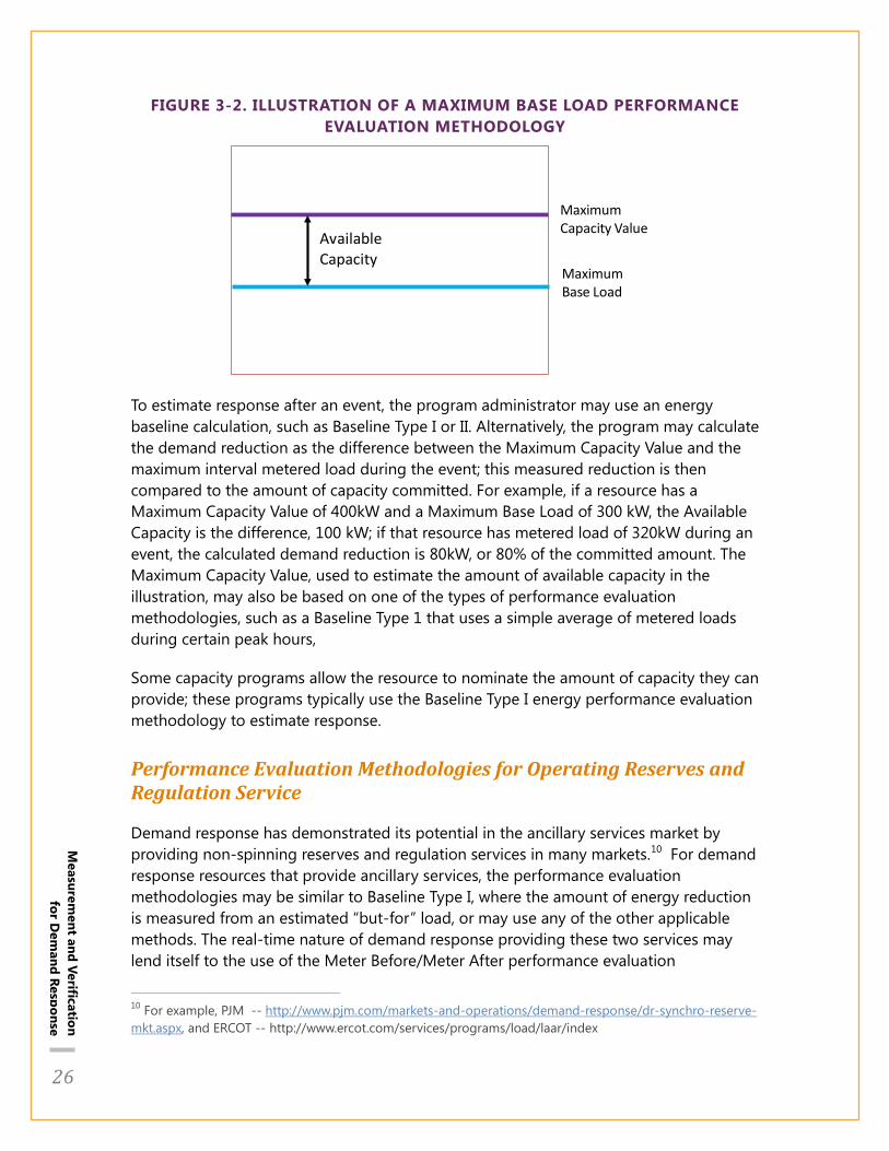
26

Measurem


emand Response

FIGURE 3-2. ILLUSTRATION OF A MAXIMUM BASE LOAD PERFORMANCE EVALUATION METHODOLOGY

To estimate response after an event, the program administrator may use an energy baseline calculation, such as Baseline Type I or II. Alternatively, the program may calculate the demand reduction as the difference between the Maximum Capacity Value and the maximum interval metered load during the event; this measured reduction is then compared to the amount of capacity committed. For example, if a resource has a Maximum Capacity Value of 400kW and a Maximum Base Load of 300 kW, the Available Capacity is the difference, 100 kW; if that resource has metered load of 320kW during an event, the calculated demand reduction is 80kW, or 80% of the committed amount. The Maximum Capacity Value, used to estimate the amount of available capacity in the illustration, may also be based on one of the types of performance evaluation methodologies, such as a Baseline Type 1 that uses a simple average of metered loads during certain peak hours,

Some capacity programs allow the resource to nominate the amount of capacity they can provide; these programs typically use the Baseline Type I energy performance evaluation methodology to estimate response.

Performance Evaluation Methodologies for Operating Reserves and Regulation Service

Demand response has demonstrated its potential in the ancillary services market by providing non-spinning reserves and regulation services in many markets.10

10 For example, PJM --

For demand response resources that provide ancillary services, the performance evaluation methodologies may be similar to Baseline Type I, where the amount of energy reduction is measured from an estimated “but-for” load, or may use any of the other applicable methods. The real-time nature of demand response providing these two services may lend itself to the use of the Meter Before/Meter After performance evaluation

http://www.pjm.com/markets-and-operations/demand-response/dr-synchro-reserve-mkt.aspx, and ERCOT -- http://www.ercot.com/services/programs/load/laar/index

Available Capacity

Maximum Capacity Value

Maximum Base Load

http://www.pjm.com/markets-and-operations/demand-response/dr-synchro-reserve-mkt.aspx�

http://www.pjm.com/markets-and-operations/demand-response/dr-synchro-reserve-mkt.aspx�

27

Measurem


emand Response

methodology, where change from a previous interval is measured, similar to a traditional supply resource. At the time of this report, the penetration of demand response providing ancillary services and details on common performance evaluation methods for these services are limited.

3.4. APPLYING THE NAESB M&V TERMINOLOGY TO COMMON DEMAND RESPONSE PROGRAM CONCEPTS

Administrators of demand response programs may initially find it challenging to categorize their performance evaluation methodologies using the NAESB terminology. Table 3-3 lists some of the more common types of demand response programs and how those programs or program mechanisms align with the NAESB terminology and whether further discussion of the demand response program or program mechanism is included in this document. This summary indicates common examples and is not meant to be exhaustive of possible M&V applications to program mechanisms.

28

Measurem


emand Response

TABLE 3-3. SUMMARY OF COMMON DEMAND RESPONSE PROGRAM MECHANISMS

Program Mechanism

Market/Service Type

Resource/ Customer Type

Applicable NAESB DR

M&V Method

Further Guidance in this Document

Firm load: Reduce to

pre-specified load on

notification


Any Maximum Base Load Evaluation

Impact Estimation Approaches

Reduction from baseline

Retail (incl. Peak Time Rebate) or Wholesale/Energy, Capacity, Reserves


Baseline Type 1 (interval meter)





Reduction from baseline, short events

Retail or Wholesale/ Reserves


Meter Before/ Meter After

None



Application of Meter Before/ Meter After for sample

Behind-the-Meter Generation


Customer-sited generation

Metering Generator Output

Baseline methods applied to generation

Direct Load Control

Retail Individual end users

N/Aa Impact Estimation approaches

Direct Load Control

Retail or Wholesale Aggregate of retail participants

Baseline Type 1 or Type 2

Impact Estimation approaches

In this table, a “Retail” market or service refers to a program or service operated by a load serving entity or DR aggregator to serve end use customers; . A “Wholesale” market or service refers to a program or service operated by a wholesale market operator. In each case, the applicable DR M&V methods are the methods the operator

29

Measurem


emand Response

would use to measure performance of the DR provider. A retail program may be offered as an aggregate DR resource in the wholesale market. Different M&V methods may be used for retail settlement than for wholesale settlement, or for determination of demand reduction quantities for individuals than for aggregates. Direct Load Control (DLC) is not ordinarily offered by wholesale markets. Wholesale Direct Load Control in the table refers to aggregated DLC participating as a DR resource in a wholesale market. While NAESB Baseline Type 1 could in principle be applied to individual DLC end users, this practice is neither common nor recommended for retail settlement.

As indicated in the table, guidance in this document focuses primarily on specification of baseline methods, and on program-level impact estimation, We turn first to methods for settlement, which are primarily baseline methods.

3.4.1. Firm load Demand response programs that require participants to reduce load to a pre-specified, individually negotiated “firm” level during the event window, upon notification from the program administrator are effectively using the Maximum Base Load performance evaluation methodology. For many of these programs, M&V for settlement with the participating load is a straightforward observation of how much the load exceeded the firm level. Typically this determination is based on the maximum metered load during the event window.

3.4.2. Reduction from baseline Many DR programs require participants to reduce load relative to a baseline during a performance window after notification by the program administrator. These DR programs reward participants according to the amount of their demand reductions during that window. These programs include many wholesale demand response programs, and retail programs, including Peak Time Rebate programs.

For a participant that is an individual end user with interval metered load data, the baseline is calculated from the participant’s individual interval load data and settlement is usually based on the magnitude of the reduction. This is an application of the NAESB Baseline Type I method.

For a demand response program that permits the aggregation of individually metered end users, an aggregate baseline may be calculated from the aggregate of the individual end users’ interval load data and compared with the aggregate observed load to determine the demand reduction. Alternatively, the aggregate demand reduction may be calculated as the sum of individual end user reductions, each calculated from its own

30

Measurem


emand Response

baseline and own actual load. These are also applications of the NAESB Baseline Type I method.

For a participant that is an aggregate of individual end users who are not all on interval meters, interval metering may be required for a statistical sample of the end users. The baseline is calculated from the interval load data for the sample. This is an application of the NAESB Baseline Type II method.

For short term demand reductions, such as ancillary services, NAESB Meter Before/Meter After method may be used, and may be used in conjunction with another performance evaluation methodology to ensure the best estimate of the response and to mitigate gaming opportunities. The method can be used directly when the end user(s) all have individual interval metered load. Although not in widespread use at this time, it is possible that for an aggregation of end users who do not have interval metered load, Meter Before/Meter After can be applied to the aggregate load estimates from a statistical sample of end users. The use of data from the sample makes this approach an application of the NAESB Baseline Type II method in combination with Meter Before/Meter After.

3.4.3. Behind-the-Meter Generation If the use of behind-the-meter generation is permitted in the demand response program, specific performance evaluation methodologies may apply to the output of the behind-the-meter generation during a demand response event or schedule. The applicable NAESB DR M&V method is Metering Generator Output. However, depending on how the participant uses the generator absent an event, a baseline calculation may still be needed. The same performance evaluation methodologies that are used for load participating as a resource may be applied to behind-the-meter generation. The value contributed to the program is measured as the difference between the metered generator output and the baseline generation for the event window. For wholesale demand response, measuring only the metered generation does not capture the impact of the total demand response resource’s load on the wholesale power grid. As a result, Metering Generator Output may be used in combination with another performance evaluation methodology when the demand response resource reduces load in addition to its behind-the-meter generation. Or, metering at the retail delivery point may be used in lieu of separate metering of the behind-the-meter generator.

3.4.4. Direct Load Control (DLC) Direct load control (DLC) programs allow the program operator to control customers’ equipment directly via communicating technology that signals equipment to turn off and then releases the control at the end of the event window. Initially, control devices were radio-signaled switches that turned equipment off entirely or limited how much the

31

Measurem


emand Response

equipment could run in each hour. Most commonly controlled equipment types were residential central air conditioners, water heaters, pool pumps, or heat pumps. More advanced control equipment includes re-setting thermostats rather than restricting equipment duty cycle, and two-way communication to allow customers to over-ride control and programs to record customer control status.

Most DLC programs do not pay individual participants for their individual amounts of load reduction. Rather, as noted above, payment is typically some type of fixed participation credit per season, event, or event hour. As a result, DLC programs may not require measurement of reduction amounts as a basis for settlement between the retail program and the end-use participant. However, to determine the amount of credit to provide or to determine the benefit of the program, an estimate of the aggregate load reduction is needed and this can be determined using a baseline.

If the total DLC program reduction is offered into a wholesale market as a demand response resource, a method for determining the reduction quantity during each event is necessary for settlement of the program with the wholesale market. Currently, DLC performance in wholesale energy markets is measured using a variety of methods, discussed in Section 4. Some of these methods can broadly be interpreted as applications of Baseline 1 (for customers who all have interval metering data) or Baseline 2 (when a sample of customers is metered).

32

Measurem


emand Response

4. M&V Methods for Settlement

4.1. FUNDAMENTAL METHOD DESIGN CONCEPTS

Designing a performance evaluation methodology for demand response program settlement starts with basic criteria:

Accuracy – the method should provide an accurate estimate of the load so that demand response resources are credited only for load reductions associated with the event and baseline manipulation is minimized.

Flexibility – the method should provide an accurate estimate of the load for all types of demand response resources that are expected and take into consideration extraordinary circumstances such as excessively high load on event days and exclusions that may reduce the accuracy of the estimate.

Simplicity/Comprehensibility – the method should be able to be conveyed in straightforward language so that the requirements and calculations are readily understood

Reproducibility – the performance evaluation calculation should be reproducible by the demand response resource, aggregator and program impact evaluator

The criteria outlined in the NAESB Business Practice Standards for Measurement and Verification for demand response were developed to provide the structure for designing performance evaluation methodologies that support these fundamental criteria. The performance evaluation methodology used for settlement of the demand response program is vital to the success of any demand response program; being able to estimate the available reduction capability and making payment for the amount of reduction at the time of the event are key aspects of demand response programs.

As illustrated in Figure 4-1, DR M&V methods and results affect and are affected by many aspects of program planning, design, and operations. The M&V method specification for settlement, program structure and rules, and cost-effectiveness analysis all need to be considered jointly as part of program design.

33

Measurem


emand Response

FIGURE 4-1. DR M&V METHODS AND RESULTS AFFECT AND ARE AFFECTED BY MANY ASPECTS OF PROGRAM PLANNING, DESIGN, AND OPERATIONS

Program rules, including measurement methods, payments, and penalties based on those measurements, affect the types of participants that will be interested in joining and staying in the program. Program rules also specify the conditions under which events are called, which can affect the results of M&V. M&V results and the accuracy of those results depend on the operating conditions as well as on the participant characteristics and M&V methods themselves. The M&V results may be incorporated into planning and forecasting, as well as the assessment of the program’s cost-effectiveness. Cost-effectiveness is the assessment of whether or not the benefits of the program outweigh its costs. Inaccurate M&V can result in over- or under-paying program participants and affect the level of program costs,program participation (i.e., over-paying will likely attract participation, and under-paying may reduce participation), and benefits computation. Over-estimated savings may result in over-stated benefits of avoided generation costs, which also reduces the benefit/cost ratio.

M&V method specification is an iterative process, as is all program design. After the initial design and implementation, modifications are suggested based on experience. Participant enrollment levels and behavior change in response to those program changes. The program rules and measurement methods must be re-evaluated and potentially revised based on customer response to changes in program design.

34

Measurem


emand Response

The remainder of this section addresses baseline method specification for settlement. This specification is a primary challenge for designing DR programs that settle based on measured reductions. We first review the elements of baseline estimation error, and general means of managing those errors. We then discuss how the characteristics of participating resources and program rules can affect DR M&V accuracy. For each set of issues discussed, we provide recommendations.

4.2. LOAD CHARACTERISTICS THAT AFFECT DR M&V CHOICES AND ACCURACY

As described in Section 3, baseline calculation methods are specified by the combination of the data selection rules (baseline window and exclusion rules), the calculation type, and the adjustments (adjustment window and baseline adjustment method).

Simple baseline calculations support transparency. A variety of simple baselines are in use, using as the calculation method a simple or rolling average of load in each hour over days in the baseline window, subject to exclusion rules. Often an additive or scalar adjustment to recent pre-event hours is also included. Examples of such methods are included in Appendix B.

Empirical studies of baseline accuracy for commercial and industrial customers have shown that many simple baseline methods of this type for individual loads can have acceptable accuracy for program operations under a wide variety of loads and conditions. These studies have also found that, as long as a symmetric day-of adjustment is included, regression-based methods are no more accurate than these simpler averages. Additive adjustments are generally preferred to scalar adjustments, because the resulting baseline can become volatile under a scalar adjustment.

For residential customers, however, simple baselines based on averages of recent eligible days have been found to have substantial biases for individual customers and, to a lesser extent, for program-level aggregates.11

The types of loads participating in the DR program affect the types of baselines that can be effective, and the issues that need to be addressed in designing the program rules

These biases are somewhat mitigated but are still substantial when day-of adjustments are used. While there are potentially ways to improve on these baselines, effective alternatives with much lower errors include the use of unit estimates based on prior evaluation work that incorporates more complete weather regression modeling, and the use of experimental design. Use of experimental design is discussed later in Section 4 and further in Section 5.

11 See Oklahoma Corporation Commission Staff Report, Assessment of a Peak Time Rebate Pilot by Oklahoma Gas & Electric Company. Prepared by Dr. Stephen S. George, November 2, 2012.

35

Measurem


emand Response

and baseline methods. Issues and methods associated with different load characteristics are discussed in what follows.

4.2.1. Business or customer type Business or customer type affects baseline accuracy primarily through its operational characteristics. Thus, if baseline methods are to be assigned based on customer type, this assignment is most effective if it is based on observable load characteristics, rather than a reported business category. For example, as noted, an industrial customer might have very consistent, non-weather-sensitive load patterns, weather-sensitive but otherwise consistent patterns, or highly variable patterns. Different methods will be most effective for these different customer types.

There are, however, broad differences between customer classes that relate to baseline method accuracy. Air conditioning tends to be a larger fraction of summer load for residential customers than for commercial customers, and many industrial customers have minimal weather sensitivity. Residential customers also use air conditioning more variably. Both these factors can make baseline accuracy more of a challenge in the residential sector compared to larger customers, for programs directed to summer peak use.

Recommendation: business or customer type

If baseline methods are to be assigned based on customer type, this assignment is most effective if it is based on observable load characteristics and broad revenue class, rather than on a reported business category or customer segment.

Key qualities that can be determined from the customer’s load data include:

Weather sensitivity

Seasonality unrelated to weather

Variability unrelated to season or weather.

4.2.2. Weather sensitivity Residential and small commercial customers tend to have more weather sensitivity than large industrial loads. However, some large industrial facilities do include substantial weather sensitivity.

For weather-sensitive loads, it is particularly important to have days in the baseline calculation from the same season and with similar weather. In particular, as discussed above if events are called or bids clear on all hot (or cold) days, the accuracy of almost any baseline method is likely to be poor for weather-sensitive loads.

36

Measurem


emand Response

Baselines for moderately weather sensitive loads work best when they include symmetric adjustments that reflect the weather of the event day. Without a day-of-event adjustment, reductions on very hot (or very cold) days can be substantially understated. This understatement occurs even if recent days are used and only higher-load days are included in the baseline computation.

Day-of-event adjustments will tend to over-state reductions for customers who pre-cool/heat in response to notification or in anticipation of a likely event. Customer-specific symmetric adjustments tend to understate reductions for customers who cancel work shifts before an event in response to notification. For this reason, it is recommended that adjustments rely on observed load in a time interval prior to the time of notification, or else use system or weather characteristics rather than the participants’ pre-event load.

A common type of baseline is a simple average for each hour, taking the highest-load subset of X days in the baseline window of Y days. This “High X of Y” approach selects for days that are more like a peak day when events may be more likely. For weather-sensitive loads, however, this type of baseline still tends to understate baselines and corresponding load reductions on extreme hot days. On the other hand, “High X of Y” baselines will tend to be overstated on event days that are mild compared to recent days.

The inclusion of a day-of-event additive adjustment will substantially correct the understatement on peak days and the overstatement on mild days, though the load at the peak hours will still tend to be somewhat under- and over-stated in these respective cases.

Day-of-event adjustments do have some limitations (discussed later in this section, in Shift cancellation and other operational response to event notification or anticipation). Weather-based adjustments reflecting the load’s historical relation to weather have been implemented successfully and provide an alternative for these scenarios (PJM weather sensitive adjustment method is discussed later in this section in Notification Rules and day-of-event adjustments, and in Appendix B). For residential customers with substantial weather sensitivity, baselines based on averages of recent days have been found to perform poorly, even with day-of-event adjustments. To calculate program-level reductions for programs with large numbers of homogenous customers, effective alternatives with higher accuracy are experimental design, or use of unit savings calculations determined from prior studies using regression analysis.

Recommendation: Weather-Sensitive loads

To reduce biases for moderately weather-sensitive commercial/industrial loads, include a symmetric day-of-event adjustment. Where anticipatory load changes are considered to be likely for many participants, a weather-based adjustment not affected by the customer’s event-day load in pre-event hours should be considered.

37

Measurem


emand Response

For program-level reductions for programs with large numbers of homogenous customers, use either unit savings calculations determined from prior studies using regression analysis, or experimental design.

4.2.3. Seasonality Some loads have seasonal variations in operating patterns unrelated to weather. For such loads, baseline calculations that depend explicitly on weather variables, such as degree-day regressions or the PJM THI adjustment method, could create distortions. However, it is important to ensure that the data used in the baseline calculation are from the season of the event day.

Recommendation: Seasonal Non-Weather-Sensitive loads

To reduce biases for seasonal, non-weather-sensitive loads, include a symmetric day-of-event adjustment that is not explicitly related to weather terms.

4.2.4. Operational Variability—Highly Variable Loads

Some loads are very consistent for a given day, hour, and season, or can be well predicted using weather variables. Other loads are highly variable in ways that are not readily described by calendar and weather factors.

Loads that are highly variable apart from systematic weather response are a challenge for any performance evaluation methodology. For such assets, general customer baseline methods tend to produce demand reduction estimates with limited relationship to actual DR actions. The resulting disconnect between actions taken and payments to the participant can result in participant dissatisfaction, as well as detracting from market efficiency. If there are no penalties to the participant for under-performance, the highly variable asset is likely to stay in the program and receive erratic payments, without necessarily providing value to the market.

If a DR program is open to customers with highly variable loads, one strategy is to include a non-performance penalty to discourage customers who are unlikely to have a meaningful baseline from participating. Other strategies have been the subject of informal discussions by practitioners, but do not necessarily have any experience as of yet.

One potential strategy is to allow a procedure for customized baselines, to shift more of the prediction burden to the participant. For example, a customer may know what factors affect its load variations, and may be able to provide operational data that allow a more meaningful baseline to be constructed. The customer would then be required to submit

38

Measurem


emand Response

its planned levels of these operating conditions prior to bid submittal or the event notification. A simple example is that a plant with frequent, irregular shutdown periods might be required to provide advance notice of a pending shutdown, and would be penalized for shutting down without prior notice if there is no DR event called.

Alternatively, the customer would be required to offer its own load prediction. If the participant is providing predictions of operations or load that will be the basis for calculating a baseline for settlement, the participant must also face a penalty if actual operations or load depart substantially from the prediction if a load reduction is not called. This approach is not currently in use, and details remain to be developed.

Another strategy is to establish formal criteria for measuring the predictability of a participant’s load. Assets whose load does not meet the predictability criteria either would not be allowed to participate, or would have their calculated reductions de-rated. A variant of this approach would be to count load reductions only if they are beyond an uncertainty band for the baseline.

Highly variable loads are inherently problematic for baselines intended to represent the load absent the DR event. In terms of program operations and settlement with the participant, such loads may be better engaged in other DR strategies, such as critical peak pricing or a firm load requirement program. Even if baselines are not needed to operate those other types of DR, impact estimation of DR performance from highly variable loads remains a challenge for all program types.

Many program operators must accept any eligible customer, and do not actively target, encourage, or discourage particular participants. For those operators, the only means of restricting or directing customers is through meaningful and defensible program rules.

Recommendations: Highly Variable Loads

For resources with highly variable loads, to ensure that incentives payments are meaningfully aligned with demand reduction actions taken, the following strategies may be considered:

Establish a “predictability” requirement for program eligibility.

Allow a customized baseline that uses additional operational information supplied by the participant.

Require the participant to provide its own baseline prior to notification, and penalize large departures from the participant’s “scheduled” load on non-event days.

If allowed, encourage the customer to participate in other types of DR programs that do not require calculation of demand reduction for program settlement.

39

Measurem


emand Response

4.2.5. Presence of Facilitating Technology It is generally recognized that facilitating technology that allows customers to respond automatically to an event signal increases the responsiveness of participating customers. Automating technology also makes participation more attractive to customers. To a certain extent, facilitating technology can also improve the quality of M&V. A customer with effective control systems in place will tend to have more consistent operations during non-event periods, and more consistent response to events.

The control systems also may offer the opportunity to record additional operating parameters that can be useful in a more comprehensive impact estimation, or for other aspects of settlement not associated with baseline calculations. At a minimum, the program operator will typically have data on when control signals were sent. If the control signal technology is two-way, the operator may also have data on signal receipt and over-rides, if that is an option. Payments to customers can then be adjusted for failed signal receipt or over-rides. For example, some direct load control programs using two-way communicating thermostats allow customers to over-ride the thermostat re-set signal, and the customer pays a penalty or gives up an incentive payment for doing so. As described in Section 5, this system information on signal receipt and over-ride can be used for impact estimation, and for settlement based on ex ante unit savings and the number of units.

Recommendation: facilitating technology

For load control programs settled in the wholesale market based on the number of units controlled, information from the control system on control over-ride, success, or magnitude should be used as an input to the settlement calculation.

4.2.6. Shift Cancellation and Other Operational Response to Event Notification or Anticipation

As discussed above related to notification and adjustment timing, different types of customers have different inclinations to modify their load in preparation for or anticipation of a DR event. Participants who have to deal with shift scheduling will have different pre-event behavior from those who can turn major loads on and off on short notice. For customers with substantial heating or cooling of the premise or energy storage capability, pre-heating or pre-cooling is a consideration for baseline accuracy.

Some plants want to be able to respond to a DR notice by canceling a shift that is scheduled to start well before the event window. If the adjustment window would include part of the cancelled shift, the plant’s baseline will be reduced by the shift cancellation. For this reason, it is recommended that participant-specific adjustments are based on pre-notification periods. For demand response resources that participate

40

Measurem


emand Response

through offers to the market, consider allowing participants to specify a notification/start up time as part of their offer.

A plant with stable operating patterns and no weather sensitivity is likely to be better represented by a baseline with no day-of-event adjustment. Using the unadjusted baseline would allow the plant to cancel shifts before the event window without a negative effect on its calculated reduction.

Long-term shutdowns may affect the baselines of demand response resources in programs where historical data from a prior period, such as the same season in the prior year, is used in a baseline calculation. Establishing procedures for reporting such planned shutdowns in advance can reduce opportunities for a baseline to be overstated.

4.2.7. DR Resources Providing Load Reduction Every Day

In principle, any demand response resource with a capacity obligation must be available to provide demand reduction during all times covered by its obligation. Otherwise, demand response used as a capacity resource may not be able to displace the need for generation capacity – i.e., additional generation may need to be acquired to cover the hours that demand response resources were unavailable. Likewise, entities offering demand resources typically want to minimize restrictions on their opportunity to sell this service.

Some demand response resources are indeed in a position to provide demand reductions consistently every day. For example, a customer with behind-the-meter generation potentially could use its own generation, within the constraint of environmental permitting rules, to reduce load taken from the market on as many days as required by DR calls, but otherwise use its own generation only in emergencies. Even without onsite generation, a facility might have the ability to shift loads such that it could go to a lower level of operation during any period called, on any number of successive days, but would stay at a higher operational level if not called.

Meaningful measurement of load reduction requires observation of “non-dispatched” operating conditions. A resource that is in reduction mode on a continual or daily basis no longer has a “no-dispatch” state of operation against which the reduction can be measured. However, setting explicit rules to limit how frequently a resource may offer reductions is at odds with the principle of resources being available across all times covered by the DR program.

To address this issue, ISO NE has established rules that limit the number of successive days on which an entity can participate as a demand resource before its baseline must be refreshed. Baseline refreshment means inclusion in the baseline calculation of meter data from a present operating day, even if the operating day included a dispatched load

41

Measurem


emand Response

reduction—in this case, meaning that the resource was instructed to reduce load as a result of its demand reduction bid clearing in the energy market.12

Further exploration is needed of mechanisms for ensuring that adequate “non-dispatch” days are available for baselines, and to assess how many days are “adequate.” Such studies can lead to guidance on the types of mechanisms to use and how to specify them in detail based on program experience.

The extent to which this rule is sufficient or excessive and its applicability to other systems and services are open empirical questions.

4.3. PROGRAM DESIGN FEATURES AFFECTING M&V CHOICE AND ACCURACY

As described in Section 3, performance evaluation methods using Baselines are specified by the combination of the data selection rules (baseline window and exclusion rules), the calculation type, and the adjustments (adjustment window and baseline adjustment method). All of these specifications are part of the program design. Other program rules affect how frequently and under what conditions events can occur, or the frequency that a demand reduction bid from a particular asset can clear in a market that incorporates DR in its energy market. The combination of these program rules and baseline specification, along with the characteristics of the participating loads discussed above, affect the baseline accuracy. Program design elements are discussed below in terms of their interaction with baseline rules and accuracy.

4.3.1. Rules to Ensure “Comparable” Days in Baseline Calculations

The baseline window is specified to select days that are in some sense similar to the event day, such as recent business days. Exclusions are sometimes applied to eliminate anomalously high or low load days. Typically, event days are also excluded from baseline calculations, since the baseline is intended to represent a participant’s consumption absent the event. Depending on the program rules and operating practices, these selection approaches can lead to a shortage of similar days in the baseline calculation, as described further below.

12 See ISO New England Inc., Docket No. ER11-4336-000, Order No. 745 Compliance Filing (Part 1 of 2) (August 19, 2011), Exhibit C to Attachment 5 “Analysis and Assessment of Baseline Accuracy: Final Report,” KEMA. http://www.iso-ne.com/regulatory/ferc/filings/2011/aug/er11_4336_000_prd_filing.pdf

42

Measurem


emand Response

Challenges if DR is dispatched on every extreme day

A common challenge is that DR events are often called on system peak days, which tend to be particularly hot summer days or cold winter days. The weather on recent non-event days will typically not be as extreme as on event days. If dispatchable events are called, or a particular bidding asset clears, on all of the most extreme weather days, it is difficult for any baseline methodology to provide accurate baselines for weather-sensitive loads for those days. This situation is a problem for impact estimation as well as for settlement baselines.

Baltimore Gas & Electric (BGE) addresses this issue by including weekends in the baseline calculation for a residential Peak Time Rebate (PTR) rate that has events only on weekdays, to ensure inclusion of hot days for each customer.13

As described earlier in Section 4.2.2, Weather Sensitivity, baseline methods based on averages of recent days, even with day-of-event adjustments, will tend to understate baselines on extreme weather days, and overstate on mild days, for highly weather sensitive loads. For weather-sensitive loads where this type of baseline is used, program rules that result in event days on a mix of extreme and mild weather days tend to produce a mix of over- and under-stated load reduction estimates. This mixing does not improve the accuracy of load or financial settlement for any single day, but can improve the overall accuracy over a season. Of course, how over- and under-stated reductions translate into net financial errors depends on the prices that apply to the different days.

An alternative approach, if program operators have discretion on when to call an event, is to operate the program in a way that ensures some event days and some non-event days for extreme weather conditions, as well as for mild conditions. For homogeneous customer groups, experimental design methods discussed in Section 5 can provide this structure.

If extreme weather days occur in sequential clusters, leaving one or more of the days in the cluster as a non-event day can partially improve the baseline accuracy for the event days that are called.

Recommendation: Program operation to reduce baseline error for weather-sensitive loads

To improve the overall accuracy of settlement for weather-sensitive loads, if the baseline method is an average of recent days with possible exclusions and day-of-event adjustments, program dispatch rules that allow the following can be considered.

Ensure that events are likely to be called on a mix of extreme and mild weather days.

13 http://www.bge.com/myaccount/billsrates/ratestariffs/electricservice/ Electric%20Services%20Rates%20and%20Tariffs/Rdrs_26_27.pdf

43

Measurem


emand Response

If extreme weather days are projected over several days in a row, leave one or more of these days as a non-event day.

Even if there are no strings of sequential extreme days, ensure that some extreme days are not called as event days, for eventual impact evaluation.

For residential programs, include weekend days in the baseline calculation even if they are not program-eligible days.

For all but the last of these, a trade-off that must be recognized is that these practices to improve baseline accuracy would come at the cost of restricting the use of the DR resource.

Challenges from too few recent non-event days -- Static baselines

For loads that vary seasonally, whether or not they are strongly weather sensitive, a related problem is frequent DR events. In demand response programs based on bids submitted by the demand response provider, some program rules may make it possible to bid in such a way so that events are called on every program-eligible day for several months. When event days are excluded from baseline calculations, as is commonly done, the result is a baseline frozen at the point before the string of DR event days began. In this case, there may be too few recent non-event days to provide the basis for an accurate baseline.

This problem will be partly ameliorated by use of a symmetric day-of-event adjustment, which roughly aligns the load level to conditions of the event day prior to the event. Day-of-event adjustments do not, however, address the changes in shape of the baseline over time. As a result, even with an adjustment, bias can increase as the source of baseline data become more distant from the event.

The frozen baseline phenomenon arises with the combination of:

DR assets clearing every day in a bidding program

Event days excluded from the baseline calculation

Weather sensitive DR assets.

In an example provided by ISO NE,14

14

several DR assets showed a pattern of bidding into the market every day at a price point that virtually assured they would be cleared, starting in the first cool period in the fall and continuing through the winter. Because these assets cleared every day, and prior event days were excluded from baseline calculations, baselines were fixed at their summer load levels. Thus, the assets received payments for the difference between summer and fall/winter load levels, even if they made no reduction in response to their bids clearing.

http://www.iso-ne.com/committees/comm_wkgrps/mrkts_comm/mrkts/mtrls/2011/jun22011/ a2c_a2d_kema_presentation_06_02_11.ppt

http://www.iso-ne.com/committees/comm_wkgrps/mrkts_comm/mrkts/mtrls/2011/jun22011/�

44

Measurem


emand Response

At the time, ISO-NE had an “asymmetric” day-of adjustment, meaning the adjustment was applied if it would increase the baseline, but not if it would decrease it. This adjustment method exacerbated the issue. Analysis of simulated load reductions and baseline calculations15

Thus, program rules can limit opportunities for static baselines by avoiding or limiting any of the bulleted conditions above. For example, ISO NE proposed incorporating cleared days (i.e., prior event days) to address baseline bias resulting from clearing every day. In this case, the main objective was to address the baseline bias

performed with program data explored the potential for frozen baselines. This analysis determined that applying a symmetric rather than asymmetric adjustment decreased the extent of the bias substantially, but did not remove bias completely. The weather sensitive load shape underlying the static summer baselines remained quite different from the fall and winter load shapes and continued to show reduction according to the baseline calculation, where no true reduction had been made. The simulation data indicated that changing the baseline method to require a minimum number of program-eligible baseline days prior to the events would more effectively address this bias. Other alternative design criteria, such as changing the exclusion rules may provide a solution to reduce the likelihood of a static baseline when demand response is deployed frequently.

Recommendations: Limiting Static Baseline Opportunities

To limit opportunities for “static baselines,” the following approaches can be considered.

1. In programs where other program rules and requirements allow, and where event days will be excluded from baseline calculations, limit how frequently a given asset is allowed to clear or to have events.

2. Incorporate event days or recent non-eligible days in the baseline calculation for assets that have too few recent non-event days in their baseline window. This should only be used in extreme situations, as doing so may increase the bias of the baseline calculation, reducing its accuracy and further understating the estimate of the load.

3. For programs that have the flexibility to target particular types of customers, target loads with minimal weather sensitivity or other seasonality. This approach is not practical for all programs, but for large, non-seasonal industrial facilities, the static baseline phenomenon is unlikely to be a problem.

To determine if a static baseline may be an issue for program participants, model the proposed baseline calculation under extreme scheduling conditions to test its resilience to frequent scheduling. If a persistent bias develops under these conditions, one of the solutions listed above may be necessary to avoid paying for non-existent load reduction

15 Simulations are discussed at length in Section 4.5.

45

Measurem


emand Response

4.3.2. Notification Rules and day-of-event adjustments

Day-of-event adjustments are often included in baseline calculations to align the baseline calculated from recent non-event days with the conditions of the event day to improve the estimate of the “but-for” load level. The typical adjustment shifts or scales the baseline by a fixed amount so that it matches the actual load during a period before the event start (the adjustment window). This adjustment can help correct for load changes due to weather, as well as for variable operations.

In simulation studies of loads that are not participating in a DR program, symmetric day-of adjustments have been shown to improve the accuracy of a wide range of baseline calculations, including those that use explicit weather models, for a wide range of load types. However, for an asset that is in a DR program, there is the possibility that the load during the adjustment window will itself be affected by the event or the expectation of an event. The extent and nature of these effects is difficult to measure, but conceptually depends on the timing of the notification along with the specification of the adjustment window and method.

Event effects during the adjustment window can occur in a number of ways including the following:

Preparatory increase in response to notification: A building is pre-cooled to a cooler than usual level from the time of event notification up to just before the event. This is a legitimate, reasonable response that makes program participation more viable for the building. However, if the adjustment window includes hours between notification and the event, the baseline will be inflated.

Preparatory decrease in response to notification: A plant cancels a shift upon notification of an event. Facility load drops prior to the event start. If the adjustment window includes hours between notification and the event, the baseline will be substantially understated.

Anticipatory increase prior to notification: A building is pre-cooled to a cooler than usual level beginning in the early morning whenever a very hot day is forecasted, which makes a DR event likely. As long as some hot days do not have DR events, the pre-cooling can be expected to be reflected in at least some of the non-event days used to calculate the baseline. The more routine the pre-cooling is, and the more the baseline window and exclusion rules select for similarly hot days, the less bias there will be in the adjusted baseline.

Anticipatory decrease prior to notification: A plant cancels a shift based on forecast conditions that suggest a likely event. Facility load drops prior to the event start. If the adjustment window includes hours between notification and the event and symmetric adjustment, the baseline will be substantially understated.

46

Measurem


emand Response

Manipulative increase: A DR asset deliberately ramps up load during the adjustment window after event notification or based on its determination that an event is likely. The baseline is artificially inflated. This behavior may be difficult to distinguish from appropriate preparatory or anticipatory increases.

Setting the adjustment window to end prior to notification can limit opportunities for deliberate manipulation. On the other hand, the earlier the adjustment window, the less effective it may be in adjusting the baseline to estimate day-of load conditions.

Day-ahead notification is more attractive to participants who want more time to respond to events, and is common in bidding programs. With day-ahead notification, any day-of-event adjustment is subject to preparatory effects, both legitimate and manipulative.

PJM’s alternative weather sensitive adjustment16

Some programs have used asymmetric adjustments, which apply the adjustment if it will increase the baseline but not if it would decrease the baseline. This practice avoids penalizing early shut-downs, but in general creates upward-biased baselines and can contribute to static baselines, discussed above.

reflects the conditions of the event day without allowing pre-event responses to distort the baseline. This method uses a simple regression of load on whether to compare event-day weather conditions during the event window to the conditions during the baseline window at the same hours. The ratio of the regression-based load estimates for the two periods provides the adjustment. The approach has the advantage of adjusting to the event day weather conditions without requiring pre-event load to be informative. The disadvantage is that it adjusts only for weather and does not adjust for an asset’s natural, non-distorting operations on the event day.

Recommendations: Baseline adjustment methodologies by notification and load characteristics

To improve accuracy and reduce bias for almost any baseline method, use an additive, symmetric day-of-event adjustment. Table 4-1 summarizes recommended adjustment window and basis, based on the notification timing, and the likely accuracy problems remaining for different types of assets.

TABLE 4-1. RECOMMENDED BASELINE ADJUSTMENTS BY NOTIFICATION TIMING AND LOAD CHARACTERISTICS

For Load Characteristics

16 http://pjm.com/markets-and-operations/etools/~/media/etools/elrs/weather-sensitive-adjustment.ashx

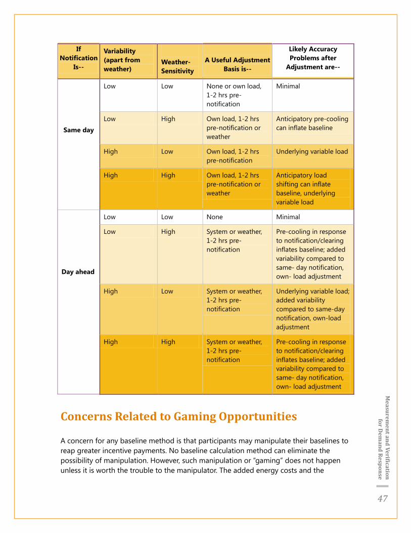
47

Measurem


emand Response

If Notification

Is--

Variability (apart from weather)

Weather-Sensitivity

A Useful Adjustment

Basis is--

Likely Accuracy Problems after

Adjustment are--

Same day

Low Low None or own load, 1-2 hrs pre-notification

Minimal

Low High Own load, 1-2 hrs pre-notification or weather

Anticipatory pre-cooling can inflate baseline

High Low Own load, 1-2 hrs pre-notification

Underlying variable load

High High Own load, 1-2 hrs pre-notification or weather

Anticipatory load shifting can inflate baseline, underlying variable load

Day ahead

Low Low None Minimal

Low High System or weather, 1-2 hrs pre-notification


High Low System or weather, 1-2 hrs pre-notification

Underlying variable load; added variability compared to same-day notification, own-load adjustment

High High System or weather, 1-2 hrs pre-notification


Concerns Related to Gaming Opportunities

A concern for any baseline method is that participants may manipulate their baselines to reap greater incentive payments. No baseline calculation method can eliminate the possibility of manipulation. However, such manipulation or “gaming” does not happen unless it is worth the trouble to the manipulator. The added energy costs and the

48

Measurem


emand Response

operational inconvenience of changing load patterns simply to inflate a baseline have to be less than the expected excess payment. A DR aggregator attempting to adjust load for purposes of manipulating baselines needs the cooperation of its customers. While some end users, especially larger organizations, may find it worthwhile to follow a baseline manipulation strategy, this practice does not appear to be widespread in existing programs.

Bidding program participants typically want to know what baseline their reductions will be measured against prior to submitting a bid. This practice assures that even if the methods have biases, the participant has visibility to the results and can make an informed decision whether to offer a load reduction relative to that baseline. However, to reduce the incentive for selective bidding based on methodologically overstated baselines, the participant should not be able to submit a bid that is guaranteed to clear.

Recommendations: Limiting Gaming Opportunities

Elements that can reduce opportunities for baseline manipulation by participants include the following.

Use a baseline calculation method that’s fair on average on likely event days, absent any gaming.

Ensure that baseline calculation data include recent “similar” days, and are limited in how far back the “look-back” period can be so that data from another season cannot be used to overstate the baseline.

Use rules that have the effect of limiting participants’ ability to control or predict what days they will be called on to reduce.

Investigate load and bidding patterns that seem perverse based on customer characteristics.

Require advance notice of scheduled shut-downs.

4.4. SETTLEMENT ISSUES AND APPROACHES FOR PARTICULAR PROGRAM TYPES

The settlement issues discussed above play out in different ways for particular program types. The following is a brief discussion of M&V issues for key types of DR programs. For each, we present a general discussion of the program type and outstanding issues to be addressed. We also identify some additional general issues requiring consideration.

49

Measurem


emand Response

4.4.1. Direct Load Control As noted in Section 3, Applying the NAESB M&V Terminology to Common Demand Response Program Concepts – DLC, DLC programs typically pay incentives to participating customer based on participation only, and not based on a measurement of each customer’s load reduction. However, DLC programs offered as DR resources in wholesale markets require a basis for measuring the reduction achieved by the program for a particular event. A variety of methods are currently in use for this purpose.

Ex Ante Unit Estimates and Current Participation

With this method of measuring DLC program load reduction, an ex ante estimate of savings per participant is multiplied by the number of successfully controlled participants. The unit savings estimate may come from engineering estimates at the start of a program, or from ex post program evaluation after some experience with the program. The average reduction per unit can be based on end-use metering, whole-premise metering, or other methods.

The ex ante estimates provide the average reduction per unit, typically by time of day or for the peak hour, and possibly also by temperature condition, by customer climate zone, or by equipment capacity. The number of successfully participating units begins with the enrollment level. This participant count should be adjusted by the rate of over-ride, if allowed by the program, and by signal success rates. These adjustment factors may be estimated from prior impact evaluation, or by event-specific information collected by the DLC program’s control system, depending on the system capabilities.

Ex ante unit savings by geography, time of day, and weather condition based on analysis of multiple prior impact evaluations is the basis for PJM’s “DLC method” for wholesale settlement. This method is used to settle DLC with PJM for participants who don’t have interval metering in place as of the start of the season.

Firm Service Level

For retail customers who have interval meters, PJM uses another method, based on Firm Service level. The retail program operator determines the total peak load contribution (PLC) of its DLC participants. This PLC serves as a Maximum Capacity Level. The operator commits to reduce the total load of the participants to a Firm Service Level during events, effectively the same as a Maximum Base Load. Performance relative to this committed reduction is calculated from the sum of the metered loads of the participants during the event.

50

Measurem


emand Response

General NAESB Baseline I or Baseline II

In principle, a Baseline method could be used that calculates a simple average of recent days, with adjustment to the event day, similar to many of the methods listed in Appendix B. This approach could be applied to individual customers with interval metering as a NAESB Baseline I method, or to a sample of customers who don’t have interval metering, as a NAESB Baseline II method. However, application of these baseline methods to DLC programs for wholesale settlement does not appear to be in use currently, and is not recommended. DLC programs that control air conditioning or heating involve loads and load impacts that are highly weather dependent. Simple baseline methods generally do not represent such loads as accurately as can the weather models used for the ex ante estimates.

Experimental Design

Experimental design, or the random assignment of eligible participants to treatment and control groups, has been used in recent years as an impact evaluation method. Operating a DR program using experimental design means that during each DR event, a randomly selected subset of participants is not dispatched, thereby serving as a control group. This approach can be useful for programs with large numbers of relatively homogeneous customers, primarily residential and small commercial.

For instance, some California direct load control programs have held back a random subset of participant households from each event activation. The event- period load for these non-activated but program participant households provides a statistically unbiased baseline for those households that were activated. This approach is not directly addressed in the NAESB DR M&V Business Practice Standards, though it could broadly be interpreted as an application of Baseline II method. Experimental design applications are discussed in Section 5.2.4.

4.4.2. Peak Time Rebate Peak Time Rebate (PTR) is a retail rate or program that provides rebates to participants who reduce their use during an event window after notification that an event will be in effect has been issued. Retail settlement with participants requires a customer-specific baseline. The general baseline methods and issues described above apply in this context.

PTR often is available to smaller customers than have historically participated in DR programs (other than DLC). For these customers, reducing air conditioning use by raising summer thermostat settings can be a key part of their response strategy.

Common baseline methods used for PTR settlement are based on averages of metered consumption data from recent non-event days, with a baseline adjustment, or data exclusion rules to select hotter days. As discussed in Section 4, most of these methods

51

Measurem


emand Response

tend to understate baselines on extreme hot days, resulting in penalties or lack of reward for customers who reduced energy consumption (and consequently made themselves uncomfortable) on very hot days. Understating the baseline and associated reduction in energy usage could be expected to lead to appreciable program dissatisfaction, though this response has not been seen in recent pilots.

Smaller load reductions that get lost in the noise can also result in underpayment. Further, customers with significant day-to-day variations in energy use could receive payments for naturally lower loads on days with event windows. In general, if the scale of reductions available to the customer is small compared to the customer’s overall variation in energy usage, establishing meaningful baselines for PTR will be challenging. This problem of small responses relative to the customer’s natural variability in energy usage is exacerbated if the PTR program is established as a default rate, with many non-engaged customers.

This issue was demonstrated in analysis of a proposed default residential PTR rate,17

60% of customers would have received incentive payments based on the calculated baseline despite not reducing load at all during an event window. This would lead to incentive payments totaling $41 million each year to customers with no load reduction.

with a baseline defined as the average of the highest 3 out of the most recent 10 eligible days, beginning 3 days before the event day, with no adjustment. The analysis of customer load on twelve key summer days showed that:

Some customers who reduced their use (compared to a peak day with no event called) would receive no payment.

With this level of mismatch between actions and payments, this particular PTR program appears to provide little incentive to move this class of customers toward more efficient consumption behavior, in line with supply costs. Payments to customers who have not performed are costly to all ratepayers. Lack of payment to customers who have made reductions could to dissuade customers from responding to future events.

The mismatch might be less severe with a different baseline method. However, even with a better baseline, there will still be payments to customers who took no action and non-payments to customers who did take action for almost any PTR program.18

One reason PTR pilots have found high participant satisfaction despite baseline inaccuracies likely has to do with customer expectations.

19

17 https://www.pge.com/regulation/RateDesignWindow2010/Testimony/PGE/2012/RateDesignWindow2010_Test_PGE_20120403_234258.pdf

Customers are not necessarily

18 For a more detailed assessment of alternative baseline methods, see Oklahoma Corporation Commission Staff Report, Assessment of a Peak Time Rebate Pilot by Oklahoma Gas & Electric Company. Prepared by Dr. Stephen S. George, November 2, 2012. .

52

Measurem


emand Response

guaranteed a payment if they take certain actions, but are paid if they beat their baselines. Moreover, baseline errors are not necessarily all in the same direction for a particular customer. In terms of the monthly bill, customers who tend to take actions during PTR events tend to see savings. Customers who respond minimally, if at all, to PTR events may or may not receive payments, and are not penalized.

Whether the baseline errors are too large for a particular program ultimately comes down to the question of whether the program is cost-effective with these baselines and the associated customer responses.

Outstanding Issues for Peak Time Rebate

More study is needed to assess the accuracy of common baseline methods for the residential sector across a range of climate conditions. Future studies should include the implications for the monetary transfers and overall cost-effectiveness, under appropriate pricing assumptions.

More study is also needed on customer load and operating characteristics that make the customer a good PTR candidate. These characteristics include not only the ability and willingness to respond to events with observable demand reductions, but also predictable usage patterns outside of event days that will tend to result in stable and meaningful baselines. Understanding these characteristics can guide policies on whether and for what customer segments PTR should become a default rate.

Cost-effectiveness assessments are needed for PTR programs, based on impact estimations of load reductions actually achieved, as well as on observed customer acceptance rates from programs that have run for one or more seasons.

4.4.3. Ancillary Services Ancillary Services is a relatively new product space for demand response, thus information on common performance evaluation methods for these new DR services is limited.

The Meter Before/Meter After performance evaluation methodology may prove to be a viable method for accurately estimating the response of DR resources under real-time dispatch conditions. Clearly Meter Before/Meter After requires demand resources with relatively flat load profiles during the time period of the dispatch. If a resource has periods of ramping up or down or general variability, the meter Before/Meter After approach can over- or under-estimate the actual level of load reduction even for the shorten period.

19 “BGE’s Smart Energy Pricing Pilot,” Cheryl Hindes, PLMA Panel, November 8, 2012.

53

Measurem


emand Response

4.4.4. Programs Using New Control/Communication Technologies

New control and communication technologies that are being incorporated into demand response include:

Remote control of equipment by customers;

Automatic dispatch of demand reduction signals to customer equipment based on a price or command signal to the customer’s meter, following a customer-specified response strategy;

Communication that a control signal has been received or that specific equipment usage has been curtailed; and/or

Real-time, two-way continuous communication with a system operator for dispatch of energy and/or ancillary service products.

The same general M&V methods can be applied for settlement (as well as for impact estimation) when these technologies are used as when they are not. However, these control and communication technologies also offer additional opportunities in the settlement context for verifying demand response and in the broader contexts of impact estimation for understanding demand response patterns.

The most useful information for M&V provided by this technology is the communication back to the program operator through new DR communication standards like OpenADR (Open Automated Demand Response).20

The operator may also receive more detailed information, such as the degrees of thermostat re-set, or particular pieces of equipment put into standby mode. This type of information is not currently being used for settlement, but could be.

This information can be used for immediate verification of curtailment and identification of failed or over-ridden signals. As described in Section 5, this information can be used to determine DLC program accomplishment for wholesale settlement.

In the impact estimation and forecasting context, relating the equipment response information to empirical observations on load reductions over time allows more fine-grained forecasts of reductions for specific customers and for future customers. Comparing the equipment changed with the measured load reduction can also provide another level of verification of the load reduction measurement.

20 http://www.openadr.org/

54

Measurem


emand Response

4.5. MEANS TO ASSESS SETTLEMENT M&V ACCURACY

As noted, there is no direct measurement of M&V accuracy. Only consumption can be metered directly, not reduction in consumption. However, by using a form of load simulation it is possible to assess in general how well a particular baseline method represents what would have happened absent a DR event. The simulation calculates baselines according to the prescribed method for a set of customers and days when no DR event occurred. Comparisons to actual load during the DR event can then be made. Following are general steps for conducting such an assessment.

1. Obtain interval load data for a set of customers similar to those expected to be in the program. For an existing program, these customers might be actual participants on non-event days. For a prospective program, the customers who will be targeted, or a similar group of customers may be used. The more similar the customers used in this analysis are to the actual (likely or targeted) program participants, the more informative the analysis will be.

2. For days similar to days when DR events are likely to be called by the program, but when no DR event is affecting the study customers, use the designated baseline method to calculate the baseline for each customer and day. If events are likely to be called under a broad range of conditions, it is important to examine baseline performance for different conditions, including frequent successive deployments. If events are likely to be targeted to extreme weather days or system peak load days, it is important to examine baseline performance under these conditions.

3. For each customer in the study data set and each study day, calculate the following for one or more event hours:

a. Calculated baseline using the baseline methodology;

b. A simulated actual load reduction quantity assuming (for example) a 20% reduction from the actual load (actual load is known in the simulation exercise);

c. The simulated actual event load with that simulated load reduction quantity;

d. The simulated load reduction calculation using the baseline methodology: the difference between the calculated baseline and the simulated actual event load;

e. The participant payment or penalty corresponding to the simulated actual load reduction quantity, applying the program payment/penalty rules to the actual reduction; and

55

Measurem


emand Response

f. The participant payment or penalty corresponding to the simulated calculated actual load reduction quantity, applying the program payment/penalty rules to the calculated reduction using the baseline method.

4. Calculate the following accuracy metrics from the quantities in Step 3:

a. Difference between (3a) the calculated baseline and actual load;

b. Difference between (3d) the load reduction calculated from the baseline and the (3b) actual reduction. This metric translates (4a) the error in estimating load into (4b) the error in estimating the load reduction; and

c. Difference between (3e) customer payments or penalties based on the reduction from the calculated baseline and (3f) what those payments or penalties would be if based on the actual reduction amount. This metric translates (4b) the error in estimating load reduction into (4c) the error in estimating the financial impacts.

5. Examine the distribution across customers and days for each of these accuracy metrics in terms of parameters such as the following:

a. Systematic errors or bias: average difference between the calculated value using the baseline method and the actual value.

b. Variability: what is the typical level of error for load, load reduction, and payment quantities?

c. What fraction of customers or what types of customers showed no positive load reduction using the calculated baseline?

d. What fraction of customers would produce a baseline load estimate that would require no actual reduction to achieve a positive payment?

Examples of such studies are discussed in Appendix A. An important point that emerges from studies of this type is that a modest error in estimating the load itself can become a much larger error in the calculated reduction. For example, for a 20% actual load reduction, , a 10% error in the estimated load level is a 50% error in the calculated reduction. These errors in measuring reductions translate into misalignments between payments and actual load reduction actions. Even with these imperfect calculations of reductions and associated rewards, the DR program may still provide benefits to the program administrator and to the market.

Several simulation studies of baseline accuracy are described in Appendix A. Each of these studies examines both systematic errors and the level of random error or variability. However, there are a variety of ways to summarize the “typical” errors across multiple customers, days, and event conditions. Different studies have used different metrics in line with the general guidance above. Development of a standardized analysis and reporting approach would improve comparisons across such studies.

56

Measurem


emand Response

5. Impact Estimation Impact estimation at the program level is another instance of measurement and verification, and plays an important role in ongoing program assessment and improvement. As indicated in Figure ES-1 above, M&V methods for settlement should be considered in the context of program planning, design, and operations. In this context, program-level impact evaluation is a key element in the ongoing cycle of program development.

Impact estimation broadly speaking means determination of program effects. For DR programs, these effects can include load reductions (or load increases) related to a particular event or set of events, energy savings (positive or negative), monetary effects, and other impacts. The effects may be determined at the program level or at any level of granularity. For purposes of this document, we consider impact estimation primarily for calculation of load reductions (positive or negative) for a program as a whole or for specific customer segments (e.g., geographic regions, low income customers, etc.).

The discussion here focuses on event-based programs. To a large extent, similar issues and methods apply to impact evaluation of alternative rate designs that are not event-based. However, issues specific to the evaluation of alternative rate designs are not examined in this report.

Impact evaluation in general measures load reduction achievement, not load reduction capability. The discussion below does not address capacity markets, though results of an impact evaluation could be used to assess capacity performance.

5.1. IMPACT ESTIMATION PURPOSES AND CONTEXTS

Impact estimation is used in a variety of contexts and for a variety of purposes. The estimation can be described in terms of the following dimensions:

Purpose: how will the reduction determination be used, and by whom?

Perspective: retrospective (ex post) or prospective (ex ante).

Level of customer aggregation: individual retail customer, entire program, aggregations of customers by the DR provider, or customer segments.

57

Measurem


emand Response

Level of event aggregation: individual event, summary of events in various forms (overall averages, averages as a function of temperature, customer segment, location, etc in a projection table or formula).

Timing of impact determination (e.g., day after event, end of season, etc.).

These dimensions are discussed below.

5.1.1. Ex Post Impact Estimation and Ex Ante Impact Estimation

Ex post impact estimation determines demand reductions retrospectively. Ex post estimation for a program season or year is commonly used as part of regulatory or stakeholder due diligence to determine if a program performed as planned, and may be the basis for payments to program operators.

Ex post estimation not only provides the retrospective scorecard of what did happen, but also is typically the foundation for developing ex ante impact estimates and for understanding how to make a program perform better going forward. Explicit projections of impacts under future conditions are ex ante impact estimates.

Ex ante impact estimation provides projected demand reduction estimates for future program periods and/or for specific event conditions (e.g., normal weather, extreme weather, etc.). These projections may be functions of enrollment levels, participant characteristics, or event conditions.

Ex ante estimates also are important for assessing the cost-effectiveness of programs. DR resources have option value – that is, they are designed to be used under extreme conditions (e.g., system emergencies, high priced periods, etc.). In any given year, such conditions may not occur frequently or be as extreme as the conditions for which the program was designed. As such, for any particular year, the average impacts per unit may understate the true value of the program. Cost-effectiveness analysis using the ex post impacts specific to any particular year thus has limited use.

For programs with relatively homogenous participants such as residential programs, ex ante methods typically consist of projected savings per participant, together with projected enrollment numbers. The projected savings per participant and enrollment is likely to vary by geography and potentially other characteristics. Savings per participant also typically varies by time of day and weather conditions.

Ex ante impact estimation can be used as the basis for retrospective settlement. In this case, application of an ex ante projection table or formula to observed conditions and actual enrollment provides an ex post impact determination. For programs that allow

58

Measurem


emand Response

dispatch to be over-ridden, enrollment is adjusted by the fraction responding or projected to be responding.

For example, PJM uses the “DLC method” to settle with utilities operating Direct Load Control programs. Prior ex post impact evaluations from the PJM region were mined to determine ex ante savings per participating unit for each utility as a function of a temperature-humidity index. Under the PJM DLC method, ex post savings for settlement are calculated by multiplying this unit savings by the number of participants, and adjusting for over-ride rates where applicable.

5.1.2. Individual and Aggregate Impacts Impact estimation is typically not concerned with accuracy for individual customers so much as accuracy of aggregate estimates at the program or participant subgroup level. Even when individual customer baselines for settlement have noise and recognized biases, impact estimation for the program as a whole can demonstrate DR as a reliable, measureable resource.

Often impacts are determined not only for the program as a whole but also by participant segments defined by program options, geography, and other customer characteristics. The segment-level analysis can provide insight into conditions where greater reductions are achieved. In addition, segmentation provides a basis for more meaningful ex ante estimates as the mix of participating customers’ changes.

5.1.3. Timing of Impact Determination Comprehensive aggregate ex post and ex ante impacts may be determined after the end of each program year or season or less frequently. Seasonal impacts may be summarized in terms of the maximum, average, or total reduction over all events in the season. Future impacts, as noted, may be expressed as functions of customer characteristics and event conditions.

Many programs determine ex post impacts within a few days of each event. Some programs need immediate impact calculations for settlement with participants. Methods commonly used for settlement with program participants are the focus of Section 4.

For both program and participant operations, day-ahead ex ante estimates are important. Program operators need to know how much of each resource is likely to be delivered in response to an event call. Program participants, both DR aggregators and individual customers, need to know what their own resources are likely to deliver to make bid decisions and other operational choices.

59

Measurem


emand Response

5.1.4. Summary of Impact Estimation Applications Table 5-1 summarizes the different ways that impact estimation is used, and the associated perspectives, aggregation, and timing. The ex ante perspective refers to ex ante estimates developed from ex post impact estimations.

TABLE 5-1. TYPICAL USEFULNESS OF DR IMPACT ESTIMATION METHODS BY END-USE PARTICIPANT TYPE AND PERSPECTIVE

Purpose Perspective User Level of Customer

Aggregation

Event Aggregation

Timing

Annual or Seasonal due diligence program measurement

Ex Post Program operator, Regulator

Program or specified aggregated load

Summary over events

End of season

Settlement with individual end users


Individual account

Individual event


Settlement with DR aggregator


Aggregated load

Individual event


Day-ahead or shorter operational planning


All DR resources or targeted subset

Individual (possible) event


Daily bidding and operations


Own resource Individual (possible) event


Annual planning


All DR resources


Season ahead

Annual planning


Own resource(s)


Season ahead up to long term planning horizon

60

Measurem


emand Response

5.2. IMPACT ESTIMATION METHODS For DR programs settled based on calculated reductions, the ex post impact can be calculated as the simple sum of the demand reductions determined for each participant using the program’s settlement methods. This method is used, for example, by the NYISO for its Emergency Demand Response Program. With this approach, there is no difference between the total settled amount and the program-level impact.

Some programs, however, conduct a program-level impact estimation that does not rely on the settlement method or settled quantities. Ex post program-level impact estimation is not subject to many of the constraints of participant settlement. These constraints include the need for simplicity, rapid results, reduction amounts for each participant and event, and timely feedback to customers for an effective behavioral change program.

More accurate program-level results can typically be obtained by using impact estimation methods that are not practical for settlement applications. These methods include:

Individual or pooled regression analysis involving more complex models and data from a broader span of time than typically used in settlement calculations that may provide ex ante and ex post results from the same model;

Day matching to identify one or more non-event days that are similar to each event day, usually from a full season of data;

Incorporation of supplemental information about customers, such as survey data, end-use metering data, or program tracking data; and

Experimental Design: Treatment/control group analysis.

These methods are discussed below. This guidance document does not attempt to specify analytic forms in detail or to identify the preferred analytic approach. Rather, the advantages and disadvantages of general methods in different contexts are described.

5.2.1. Individual regression analysis Individual regression analysis fits a regression model to an individual customer’s load data for a season or year. A basic model describes load at each hour of the day (or perhaps the average for an event window) as a function of weather terms such as cooling degree-days. More elaborate models can allow the cooling degree-day base to be determined by the regression best fit, and might include calendar and day of week effects, lag terms reflecting temperature over multiple hours, and humidity. An example of a basic individual hourly load regression model is shown in Box A.

61

Measurem


emand Response

Typically, the individual regression models are fit to loads on non-event days. The model is then applied with the conditions of each event day to provide an estimate of the customer’s load that would have occurred on that day absent an event. The impact is calculated as the difference between the modeled and observed load for each hour of the event period. Post-event rebound (increased load to make up for foregone load during the event period) can also be calculated.

When load data are available for a sample of participating customers, the program-level results are estimated by sample expansion from the individual customer impacts. When load data are available for all participating customers, program-level results are the sum of the individual customer impacts.

The individual regression model can also include event-day terms, and be fit across both event days and non-event days. In this case the event effect is the difference between the model applied to the event-day conditions with and without the event-day terms in effect. Box B provides a simple example. However, unless there are multiple event days spanning a wide range of the other terms in the model, including event-day terms in individual regressions will provide no more information than the average over event days of the modeled versus observed approach from Box A.

Box B

Example of an individual hourly load regression model with event-day terms

Ljdh = αjh + βjh Cd + δjh Ed + εjdh

In this model, Edh is a 0,1 dummy variable indicating that an event occurred on day d, δjh is the event effect for hour h, and the other terms are as in Box A.

Box A

Example of an individual hourly load regression model

Ljdh = αjh + βjh Cd + εjdh

In this model, Ljdh is the load of customer j at hour h of day d, Cd is cooling-degree-days for the day, αjh and βjh are base and cooling coefficients for each hour h of the day, specific to customer j, and εjdh is residual error.

62

Measurem


emand Response

Advantages of the individual regression method are:

Results are determined for each customer, which provides a basis for richer analysis, including looking at distributions of results rather than averages only. Individual customer results can also be related to other customer information.

Meaningful results can more easily be developed for groups of customers whose load patterns are dissimilar, since each is modeled separately.

Results can be aggregated into any segments that are subsequently determined to be of interest after the initial analysis is completed.

Customers for which the basic regression structure is not a good description can be identified by model diagnostics and treated separately.

Weather response terms such as the best degree-day base can be determined separately for each customer, leading to better and more meaningful overall fits.

Ex ante results can be derived by fitting individual regressions to design or extreme temperature data and then aggregating the resulting estimates.

Results can be analyzed to understand relative customer engagement in programs that promote behavioral changes.

On the other hand, model fits for an individual customer are subject to a higher level of estimation error than are the fits from a pooled model. Examination of distributions across customers needs to take into account that the spread of observed results reflects both the spread of individual responses and the estimation “noise” or random errors.

Moreover, if event-day effects are estimated for an individual customer, these individually estimated effects can often be lost in the noise—that is, not be statistically significant—even if across all customers there is an effect. The opposite can also occur, where statistically significant effects are found for large numbers of control group customers who had no event to respond to. That pattern indicates a systematic modeling error, which would affect a pooled model just as much as it would affect the average of individual models.

In general, if the same model structure is applied with individual fits and with a pooled fit, the coefficients of the pooled fit will be approximately the average coefficients of the individual fits. This equality will be strictly true if the individual and pooled fits all use the same degree-day base and other variables, the individual fits all have the observations in the same hours, and all observations have equal weights. In particular, any bias in the individual fits will be present for the pooled fit as well.

A disadvantage of the individual regression approach is that it does not take advantage of the power of a pooled regression approach.

63

Measurem


emand Response

5.2.2. Pooled regression analysis Pooled regression analysis uses a similar model structure to the individual regression analysis, but fits a single model across a large group of participants and hours. In this case, a single set of coefficients is used to describe all customers’ average load pattern. With a pooled analysis, it is more common to include event-day terms in the regression model. With the larger pooled sample, terms that might not be well determined for an individual customer can be estimated. A simple example is illustrated in Box C.

Advantages of the pooled regression method are:

The coefficients utilize information across all customers, so that effects that might be poorly estimated by each individual regression can be well determined.

Segment level effects can be obtained by including segment indicators in the model, or by fitting the model separately by segment.

Overall results are provided even if there are some customers for which the basic regression structure is not a good description.

Ex ante estimates can be obtained directly from the event-day terms in the model.

Disadvantages of the pooled regression method include:

Segments of interest need to be identified in the model development stage, and cannot be easily estimated after the fact from the basic results.

Weather response terms are estimated only in aggregate, which can reduce the model accuracy.

The method works best when pooling is across a group of fairly similar customers, such as residential or small commercial.

Box C

Example of a pooled hourly load regression model with event-day terms.

Ljdh = µj + τdh + αh + βh Cd + δh Ed + εjdh

In this model, the terms are as in Box B, except that the parameters αh, βh, and δjh are not customer-specific but are estimated across all customers. The term µj is an incremental fixed level for customer j. This fixed effects term reduces the intercorrelation among the residuals εjdh for repeated observations on the same customer j. Similarly, the terms τdh are fixed effect terms for affecting all customers for a particular day and hour, reducing the residual correlation for repeated observations at the same day and hour.

64

Measurem


emand Response

A pooled model approach has an added degree of complexity relative to the individual approach. Even with the inclusion of customer-specific intercepts (µj) and time-period terms (τdh) there will still tend to be serial correlations and patterns in the regression residuals (εjdh). If these correlations are not appropriately accounted for, the regression estimates can appear to be much more precise than they really are, especially if many thousands of customers are included in the regressions. That is, the calculated standard errors for the regression terms and associated savings estimates may be understated.

5.2.3. Match Days Match day methods identify one or more non-event days that are similar to each event day, based on various criteria. Common bases for identifying match days for a given event day include:

Similar temperature or temperature-humidity index;

Similar system load; or

Similar customer load at non-event hours for the individual customer.

For each participating customer, that customer’s load on the match day (or average of the match days if there are multiple) serves as the baseline or reference load. Demand reductions are calculated as the difference between the (average) match day and event day load at each hour.

A key advantage of match day methods is their simplicity and transparency. In addition, for variable loads that are not well described by hourly or weather models, match day methods may be more accurate than regression models, if the matching criteria include characteristics of the individual customer’s load.

Disadvantages of match day methods include:

For loads that can be reasonably well described in terms of hourly loads and weather patterns, regression methods will tend to be more accurate. Match days are limited to actual observed days, and averages of those days. Regression models, if properly specified, effectively interpolate between particular observed conditions, and extrapolate from them. (It’s easy to construct examples of weather models that consistently understate load in extreme weather conditions. A matched day could provide a better estimate at those conditions than such a model. However, a better model that does not systematically understate load at the conditions of interest, possibly by using only data from more extreme conditions, in most cases will be more reliable than a single best-fit day. Any basis for selecting match days should, in principle, be possible to capture more systematically and comprehensively in a regression framework.)

65

Measurem


emand Response

Match day methods do not provide a direct basis for producing ex ante estimates. If a regression will be used to extrapolate from the match-day results, it may make more sense to use a regression for the ex post results to begin with.

Assessing the accuracy of a match-day estimate is more problematic than assessing the precision of a regression model. Testing for lack of fit or systematic bias is not as straightforward with a matching procedure as with an explicit model, and is not commonly included in match-day analysis. Measuring the precision or level of random variability of a match-day estimate is also not as clear-cut. It’s possible to calculate a standard deviation across match-day estimates from multiple event days, but it’s not clear to what extent this variability reflects differences in event-day conditions versus random variations on the particular event days versus particular conditions or random variation on the non-event days used for matching. If the analysis is done for a sample of customers rather than for the full population, variability across different match days does not reflect the sampling errors (that is, the differences that would be expected with the same methods if different random samples were selected). As a result, determining the true uncertainty of both ex post estimates and projections based on those estimates is challenging.

5.2.4. Experimental Design For DLC as well as other mass market programs, comprehensive interval metering offers the opportunity to use experimental design for M&V. This approach can be used to determine program-level reductions for individual events. It has begun to be used for ex post impact estimation, and offers substantial promise. As noted in Section 3, direct use of experimental design has not yet been seen as a basis for market settlement, though ex ante estimates based on experimental design may be.

Experimental design is random assignment of customers into two groups, one of which is “treated” and the other remains as a “control” group. In the case of DLC, customers enrolled in the program are randomly assigned to subgroups, and during any dispatch event one or more of the randomly assigned groups is not dispatched while the remainder are. That capability depends in part on the program’s control technology, and in part on the operational capacity of the program. Thus, an essential feature of this impact estimation method is that it must be built into the program operation.

The average demand reduction per participant is calculated as the difference between the averages for the groups that are dispatched and those which were not. An alternative calculation with this design is a difference of differences method. A baseline calculation or load model constructed for each participant, in both the dispatched and undispatched groups (treated and control groups, respectively). The impact is then calculated as the difference between the dispatched group’s modeled and observed load, minus the corresponding difference for the control group. With this approach, the departure of the

66

Measurem


emand Response

control group from its modeled load essentially provides an estimate of how the treatment group’s actual load would have been higher or lower than its model, absent a DR event.

With customers who all have interval metering via Advanced Metering Infrastructure (AMI), this type of design and analysis has been used to determine impacts of large-scale residential and/or commercial direct load control programs at PG&E, SDG&E and across multiple utilities in Ontario Canada for the Ontario Power Authority’s (OPA) peaksaver® program.21 The approach has been used also with a sample of interval metered customers prior to the implementation of AMI, for SDG&E. 22

In many contexts, randomly assigning customers to different rates or different dispatch regimes is not possible. In these cases, comparison groups of customers identified as similar to the participants after the fact are sometimes used for impact estimation. However, without true random assignment there are always unknown underlying differences between participants and nonparticipants, and these differences can bias any estimate based on comparing the groups. The remainder of this discussion focuses on the use of randomized treatment-control experimental design. In such a design, customers originally in a common pool are randomly assigned to either the treated or comparison (control) group, with minimal subsequent opportunity for customers to opt in or out of their assigned group.

The randomized control experimental design is conceptually the gold standard of evaluation approaches, but has been limited in its practical applications until recently. The practical limitations result from the fact that most full-scale program applications and regulatory contexts don’t allow for random assignment of customers to participate in a program or not. A recent exception in the energy efficiency context is behavior-based programs offering information to large numbers of randomly selected residential customers. The experimental design of the program offering establishes the basis for measuring the effect of the information program.23

Where feasible, experimental design has the potential to produce the most accurate results possible for estimating load reduction. The method is valuable because it virtually eliminates any systematic difference between treatment and control, providing an unbiased estimate, and with sufficiently large samples can provide very high precision.

21 Full load impact evaluation reports on the PG&E and SDG&E programs can be found at the following websites: http://www.fscgroup.com/reports/2011-sdge-summer-saver-evaluation.pdf. http://www.fscgroup.com/reports/2011-pge-smartac-evaluation.pdf 22 2005 Smart Thermostat Program Impact Evaluation. Prepared by KEMA for San Diego Gas and Electric Company. April 24, 2006. http://www.calmac.org/publications/2005_Smart_Thermostat_Final.pdf 23 Evaluation, Measurement, and Verification (EM&V) of Residential Behavior-Based Energy Efficiency Programs: Issues and Recommendations. Todd, A., E. Stuart, S.Schiller, and C. Goldman. Lawrence Berkeley National Laboratory. May 2012

http://www.fscgroup.com/reports/2011-sdge-summer-saver-evaluation.pdf�

67

Measurem


emand Response

Experimental design is effective for impact estimation of relatively homogeneous groups of customers, such as residential or small commercial, where several hundred or several thousand customers participate in a program. The method is less effective for evaluating smaller numbers of customers or large commercial or industrial customers, because the treatment-control differences will have too much random error to be reliable.

When most participants have interval metered data available, experimental design offers many advantages including the following:

First, because the M&V is conducted separately for each event day, participants do not have to be assigned to treatment or control permanently. In fact, it is more appropriate to have the control group be a different, randomly selected set of participants for each event. This approach best assures that the treatment and control group are the same in all ways other than being dispatched on a particular day, including that they have otherwise equivalent program experience.

Second, for a large scale program, large control samples can be used to provide highly accurate results without substantially reducing the total dispatched resource. When load control programs had to be evaluated using metering samples installed specifically for that purpose, samples on the order of a few hundred (depending on the level of granularity desired) were sufficient to provide adequate accuracy for the estimated reductions. A program with 50,000 customers enrolled could easily have a control sample of 1,000 customers for each event day to produce accurate estimates of program load reductions.

Third, for ex post estimation or for settlement directly based on the metering sample, determining savings based on a randomly assigned treatment-control difference provides a highly accurate estimate of the reduction without requiring explicit weather modeling. If weather modeling is used, the difference of differences method ensures that any systematic bias in the modeling can be corrected by subtracting the difference between the modeled and actual load of the control group from the difference between the modeled and actual load of the control group of the dispatched group.

Fourth, for ex ante estimation, observing large numbers of both dispatched and undispatched customers during each event provides a much more accurate basis for modeling event effects as functions of weather or other conditions. This type of modeling can be very challenging in particular if all participants are dispatched on the few hot days.

Fifth, as an extension of the last point, with a random control group as the basis for settlement and evaluation, calling events on every hot day does not create a problem for M&V.

Finally, the experimental design approach can allow good load reduction estimates to be developed for a wide range of conditions, while exposing any individual customer to a limited number of control events. This feature can allow the method to be used to define ex ante estimates for a range of operating

68

Measurem


emand Response

parameters and weather conditions. Implementing this aspect of the approach requires close coordination with the program operation.

The best ways to produce ex ante estimates based on experimental design are still to be explored. The per-unit results from different event days can be averaged, or a simple temperature regression can be fit to the results.24

A more complete approach could be to fit a pooled model across all customers and days. Having treated and control customers on each event day as well as having both event and non-event days for each customer strengthens this analysis. The pooled model could provide ex ante estimates per unit as a function of weather conditions.

This type of analysis is relatively straightforward to conduct with a sample of a few hundred or even several thousand participating customers, but may be computationally challenging for a large residential program with universal hourly load data available. Possible ways of addressing that challenge include:

Conduct the analysis using data from a large sample of participants, not all of them.

Aggregate the load for groups of customers who had the same DR dispatch schedule. Conduct a pooled analysis on the groups.

5.2.5. Applications of End-Use Metering for DR Impact Estimation

Until the last few years, interval load data has not been available for most small customers. Impact estimation for residential DR programs such as DLC has typically relied on metering samples installed for this purpose. In areas without AMI, that will still be the case in the future.

Since DLC programs control a particular end use, impact estimation can be conducted by metering only the affected end use(s). Many DLC evaluations have taken this approach. Advantages of end-use metering include the following:

A single end-use can typically be modeled more accurately than whole-premise data, resulting in better precision for the overall estimates for a given sample size.

Equipment operating characteristics such as duty cycle and connected load can be identified, providing additional insight into event response patterns.

Load curtailment can be observed directly if end-use metering data are collected at 1-minute intervals.

24 For an example of this, see the load impact evaluation report for PG&E’s SmartAC program for 2011, which can be found at http://www.fscgroup.com/reports/2011-pge-smartac-evaluation.pdf

http://www.fscgroup.com/reports/2011-pge-smartac-evaluation.pdf�

69

Measurem


emand Response

On the other hand, whole-premise metering captures other effects in the home that are not reflected in the end-use metering. For example, control of the air conditioner compressor could result in increased use of fans or even room air conditioners.

When interval load data are broadly available via AMI, investment in end-use metering for impact estimation becomes more difficult to justify. Moreover, the large numbers of metered customers available with AMI makes up for the reduced resolution for individual customers in an impact evaluation. However, even on a small sample basis, supplemental end-use metering can provide finer grained understanding of load response patterns and mechanisms. In particular, modeling duty cycle and connected load as functions of temperature provides a strong basis for projecting the effects of alternative air conditioner control strategies, as described below.

End-use metering data can be analyzed using the same types of modeling approaches as whole-premise data, including use of a randomized treatment/control methodology. This approach has been used for example in the evaluation of the SDG&E Smart Thermostat program.25

For air conditioner DLC, end-use metering analysis can take more complete advantage of the physical relationships that drive air conditioning. One such approach

26

1. A model that estimates the connected load of the air conditioner, the kW draw when the unit is running, as a function of current outside temperature. This connected load is not constant, but increases by 1 to 2 percent per degree Fahrenheit.

fits 2 types of models to 15-minute or finer air conditioning metering data for each unit in a metering sample:

2. A model of duty cycle, or the fraction of each hour the unit runs, as a function of daily weather conditions. The duty cycle model uses a structural form that recognizes that the duty cycle must be between 0 and 100%.

Advantages of this analysis approach include:

The analysis reveals detailed patterns of customer equipment use at different conditions.

These patterns can be related to other customer characteristics.

Projected reductions can be estimated by time of day and weather condition, at any level and strategy of duty cycle control, not just those observed in the

25 2005 Smart Thermostat Program Impact Evaluation. Prepared by KEMA for San Diego Gas and Electric Company. April 24, 2006. http://www.calmac.org/publications/2005_Smart_Thermostat_Final.pdf 26Pacific Gas & Electric SmartAC™ 2008 Residential Ex Post Load Impact Evaluation and Ex Ante Load Impact Estimates, Final Report. KEMA. March, 2009. http://www.calmac.org/publications/FINAL_SmartAC_Load_Impact_2009_03_31_-_CALMAC_Study_Id_PGE0278.01.pdf

70

Measurem


emand Response

evaluation. That is, this approach more accurately models the technical limits of AC units thus more effectively accounting for units reaching full cooling capacity at extreme temperatures.

5.2.6. Custom Engineering and Field Studies For individual large loads, special studies can be conducted to assess load impacts. These studies would typically include a site visit to identify what loads are controlled, together with end-use metering or extraction of existing operating log data to document load at event and non-event conditions. Analysis to estimate the load that would have occurred absent an event is specific to the operations of the facility. While this approach is not common, it may be the only practical method for large loads with irregular operating patterns.

5.2.7. Composite studies An approach that has been used for ex ante impact estimation in the PJM market is to consolidate the results of multiple end-use metering studies conducted for ex post impact evaluations. The consolidated metering analysis was used to develop ex ante estimates for DLC programs, for several utilities operating in that market.27

5.3. GUIDANCE SUMMARY

This approach can provide a more robust result than any single study.

Table 5-2 summarizes which impact estimation methods are likely to be most useful for different types of end-use customers, for ex post impact estimation and ex ante impact estimation. In any particular evaluation context, the methods that will be most effective will depend on a variety of factors, including specific evaluation goals, participant load characteristics, data availability, numbers of participating customers, and evaluation budget and timeframe.

TABLE 5-2. TYPICAL USEFULNESS OF DR IMPACT ESTIMATION METHODS BY END-USE PARTICIPANT TYPE AND PERSPECTIVE

Customer Type and Perspective

27 Deemed Savings Estimates for Legacy Air Conditioning and Water Heating Direct Load Control Programs in PJM Region. RLW. April, 2007. http://www.pjm.com/sitecore%20modules/web/~/media/documents/reports/20070406-deemed-savings-report-ac-heat.ashx

71

Measurem


emand Response

Impact Estimation

Method

Homogeneous Customer Group

(Residential, Small Commercial/Industrial)

Heterogeneous Customer Group, Each Customer with Low or

Moderate Load Variability

Customers with Highly Variable Loads

Ex post Ex ante Ex post Ex ante Ex post Ex ante

Individual Regression

Very useful


Useful Useful with additional work

Possibly useful


Pooled Regression

Useful Very useful Not useful Not useful Not useful Not useful

Match Day Possibly useful


Possibly useful


Useful if match on customer condition

Useful if match on customer condition, with additional work

Experimental design simple difference

Very useful


Not useful Not useful Not useful Not useful

Experimental design with modeling

Very useful

Very useful Not useful Not useful Not useful Not useful

End Use Metering with Duty Cycle Analysis

Very useful

Very useful Potentially useful

Potentially useful

Potentially useful

Potentially useful

Custom engineering and site analysis



Potentially useful

Potentially useful

Potentially useful

Potentially useful

Composite Analysis

Potentially useful

Potentially useful



Not useful Not useful

72

Measurem


emand Response

5.4. OUTSTANDING ISSUES FOR IMPACT ESTIMATION

Key outstanding issues for DR impact estimation include the following.

5.4.1. Use of Experimental Design Experimental design utilizes established statistical methods to produce unbiased, highly accurate ex post impact estimates. Key outstanding issues for increased use of this approach include:

Explore with program operators the challenges of and potential for dispatching the program following an experimental design protocol.

Work with wholesale markets to establish protocols that will allow use of experimental design as a basis for settlement.

Establish recommended strategies for developing ex ante estimates when ex post or settlement is based on experimental design.

5.4.2. Metering Options Further understanding will evolve as more studies are done on the impact of advanced

metering infrastructure (AMI) on demand response programs. Suggested work includes:

Calculate accuracy trade-offs from studies that had both end-use metering and AMI data for the same time periods.28

Incorporate lessons from prior end-use metering work to improve program-level whole-premise analysis.

Explore the value of higher frequency AMI data compared with hourly data for this type of analysis.

5.4.3. Accuracy measures Additional work is needed to establish principles and procedures for quantifying and reporting accuracy of ex post and ex ante impact estimates. Such procedures would provide more complete accounting for various dimensions of estimation error, including:

28 This work has been done in certain areas where both kinds of data have been available for many years. See San Diego Gas and Electric Smart Thermostat and Summer Saver Impact evaluation reports by both DNV KEMA and FSC at http://www.calmac.org/

73

Measurem


emand Response

variation across days, variation across end use customers, model estimation error, model lack of fit error, prediction error, and method specification error. More systematic accounting for model accuracy will provide a better understanding of DR reliability, and reduce operational risk associated with DR.

74

Measurem


emand Response

Appendix A. Prior work on DR M&V Methods In this appendix, we review prior work relevant to M&V for DR, in 2 key areas:

Method assessment studies for baselines used for settlement, and

DR Evaluation protocols.

The DR evaluation protocols are described at a high level only. We also note efforts related to the International Performance Measurement and Verification Protocol.

The emphasis of this section is on baseline methods for market settlement, as this has been a key concern for market operations.

BASELINE METHODS ASSESSMENT STUDIES

California Energy Commission The California Energy Commission (CEC) produced the report “Protocol Development for Demand Response Calculation – Findings and Recommendations” in February, 2003.29

Test data

The report was an early attempt to systematically explore the components of a baseline and compare baseline accuracy across the full range of possible baselines using actual data.

Interval load data were provided from several parts of the U.S., for both curtailed and uncurtailed accounts. A total of 646 accounts were used in the analysis. For some accounts, multiple years of data were used. The accounts used in the study were distributed across all regions of the country, the years 1998 through 2001, and curtailment/non-curtailment categories. All the regions had accounts with summer curtailment data. Only the Midwest, Northwest, and Southeast had non-summer curtailment data. Despite the fact that the report was produced for the CEC, only 4 of the 646 accounts were from California. Investigation of differences by region indicated that most differences across data sets provided appeared to be related to the types of accounts included rather than to regional variations. For this reason, results were

29 Protocol Development for Demand Response Calculation – Findings and Recommendations. California Energy Commission, February 2003. 400-02-017F.

75

Measurem


emand Response

provided separately by weather-sensitivity and degree of load variability in an account, as well as by season.

Methods tested

Methods tested were organized based on the three key characteristics of any baseline methodology:

Data selection criteria –Short, rolling windows (5 to 10 prior eligible business days) to full prior seasons of data. The rolling windows can include further restrictions based on average load (e.g., five days with the highest average load out of most recent ten);

Estimation methods –Simple averages to regression approaches using either hourly or daily temperature, degree days or temperature-humidity index (THI); and

Adjustments – Additive and multiplicative approaches based on various pre-event hours as well as a THI-based adjustment not dependent on event day load.

The analysis tested 146 combinations of data selection criteria, estimation methods and adjustments, comparing median and 95th percentiles of relative error and Theils U statistic. Results were provided for all combinations of the following characteristics: Summer/non-summer, curtailed/non-curtailed, weather sensitive/ non-weather sensitive, and high variability/non-high variability.

Key findings

The CEC report spelled out specific findings for each the three characteristics of a baseline methodology. The overarching conclusion was that no single approach offered a comprehensive solution across all kinds of account load characteristics and conditions. The report states that “baseline calculation protocols should provide for alternatives based on customer load characteristics and operating practices.” While it was recommended that customers have input into the baseline methodology based on their unique load characteristics, the program operator should have ultimate authority for the final decision.

More specific recommendations include:

A rolling ten day window with an additive adjustment based on the two hours prior to event start provides the best, most practical default baseline.

For weather-sensitive loads, limiting the rolling window to the five highest average load days is not as effective using a baseline adjustment. THI-based

76

Measurem


emand Response

adjustment is the only adjustment that avoids the distortions of pre-cooling or gaming.

Weather regression can be effective, but the increased data requirements, processing complexity and potential for changes at the site make these options less practical. Furthermore, simple averages with adjustments are nearly as good as weather regressions

Highly variable loads are a challenge regardless of the baseline methodology employed.

ISO-NE In 2010 and early 2011, ISO-NE evaluated the effect of continuous price responsive events on the accuracy of baselines. A separate analysis later in 2011 examined baseline inaccuracies in recent historical ISO-NE baselines to understand the role of load variability in the ongoing inaccuracies after the adoption of a symmetric baseline adjustment. Both analyses were performed on ISO-NE DR program populations.

Key findings, Frozen Baseline Analysis

The 2010/2011 analyses looked at bidding patterns in the Day Ahead Load Response Program and the effect on baseline accuracy.30

Conclusions from the early 2011 report included:

Participants could offer load reduction at a low enough price that their bid would clear every day. Because cleared days are removed from subsequent baseline calculations, this bidding strategy resulted in the baseline remaining frozen at the same level as the first cleared day of the series. Natural, seasonal drift made the frozen baseline increasingly inaccurate as the number of cleared days increased.

Asymmetric adjustments cause biased estimates of load reduction.

Baseline accuracy and bias are directly impacted by the frequency with which demand resources clear in the energy market. Even with a symmetric adjustment, a long-term frozen baseline leads to baseline inaccuracies.

It is possible to develop policies that improve baseline accuracy by limiting the number of days a customer can clear during a particular timeframe or requiring

30 ISO New England Inc., Docket No. ER11-4336-000, Order No. 745 Compliance Filing (Part 1 of 2) (August

19, 2011), Exhibit C to Attachment 5 “Analysis and Assessment of Baseline Accuracy: Final Report”

77

Measurem


emand Response

contemporary meter data be used in the baseline computation even if the resource clears.

Key findings Load Variability Analysis

The late 2011 variable load analysis explored a different question than the baseline comparison analyses. This analysis looked at the existing ISO-NE baseline and sought to categorize the sources of baseline inaccuracies across the program population. Conclusions included:

In absolute terms, most inaccuracy of baselines comes from a small fraction of highly variable resources.

Systematic variation by day of week as well as across hours within a single day of the week (scheduling) accounts for much of the discrepancy for the population of highly variable resources.

Additional research should include the testing of alternative baseline procedures on high variability load assets to determine if there are more accurate methods of evaluating these types of loads.

If accurate alternative baseline methods that address the potential gaming issue cannot be created, then market rules constraining the participation of highly variable loads in demand response programs will have to be developed.

California Public Utilities Commission The California Public Utilities Commission sponsored an analysis of the accuracy of baseline estimates for the California Investor Owned Utility (IOU) Aggregator DR programs.31

Individual vs aggregate application of adjustments;

These programs include the statewide Capacity Bidding Program (CBP), which is operated by all three of the state’s IOUs, PG&E’s Aggregator Managed Portfolio (AMP) and Southern California Edison’s Demand Response Resource Contracts (DRRC). The analysis tested a number of variations on the standard baseline used for the aggregator programs - a 10 of 10 day average with same day adjustment based on the first three hours of the previous four hours and capped at 20 percent. The analysis tested:

Level of adjustment cap; and

Aggregator choice of adjustment vs universal adjustment.

31 2011 Statewide Evaluation of California Aggregator Demand Response Programs Volume II: Baseline Calculation Rules and Accuracy. Freeman, Sullivan & Co. June 1, 2012

78

Measurem


emand Response

The different baseline variations were compared to ex post impact evaluation results based on regression methods and also tested on participant data using a simulated load reduction.

Findings included:

Universal application of same-day adjustments almost always increases accuracy compared to aggregator choice.

Calculating adjustments at the settlement portfolio level has a limited effect on bias but reduces the magnitude of same-day adjustments.

The effect of increasing the adjustment cap varies by program and option. When it does change results, accuracy generally improves but only slightly.

PJM In 2011, PJM sponsored an analysis of baseline options for PJM DR programs.32

Test data

This analysis ranked baseline performance based on relative error and variability as well as expected administrative costs. Where baselines delivered similar levels of accuracy, preference was given to baselines with a lower expected cost to administer.

Data were provided by Electric Distribution Companies (EDC) within PJM. Almost all EDCs contributed hourly data. The available sample of DR customers represented 39 percent of the total number of DR customers across PJM territory and 54 percent of Peak Load Contribution (PLC), load of the customers at the time of PJM’s system peak. Data were requested from 2008 through 2010.

Methods Tested The evaluation tested a range of baselines designed to represent the range of baselines

used by ISOs today. Those baselines included baselines:

Used by PJM.

Used by other ISOs and RTOs.

Suggested by the Market Monitor.

Suggested by evaluator.

32 http://pjm.com/markets-and-operations/demand-response/~/media/markets-ops/dsr/pjm-analysis-of-dr-baseline-methods-full-report.ashx

79

Measurem


emand Response

The baselines represented a range of data selection criteria and estimation methods. Four of the baselines were based on the average load of a subset of a rolling window (eg. high 5 of 10). The similar rolling ISO-NE baseline was also included. In addition there were two kinds of match-day baselines, two flat baselines and two regression-based baselines.

Four different adjustment types were applied to all of the baselines (where feasible and reasonable) including additive, ratio (multiplicative) and an additive, regression-based PJM weather sensitive (WS) adjustment. The additive and ratio adjustments were the same day load-based adjustments common across the industry. The PJM WS adjustment approach provides an adjustment based on event day weather rather than event day load. This approach avoids concerns related to same day load-based adjustments (eg., early shutdown, pre-cooling) but uses a regression-based characterization of weather sensitivity that requires additional data and computational complexity while only explicitly addressing weather as a source of variability.

Key Findings Baselines methods that use an average load over a subset of a rolling time period

(10 of 10, high 5 of 10, high 4 of 5, middle 4 of 6, and ISO-NE) with a same day additive or multiplicative adjustment performed better than any unadjusted baselines or those adjusted with the PJM WS adjustment.

These baselines all have similar results and performed well across all segments, time periods and weather conditions except in the case of variable load customers. Variable load customers should be segmented for purposes of applying a different performance evaluation methodology and/or market rule.

The PJM weather sensitive adjustment applied to the PJM economic program high 4 of 5 baseline provided the best non- load-adjusted results. This approach has the additional cost and complexity of the regression based adjustment approach.

PJM’s existing high 4 of 5 baseline with additive adjustment was consistently among the most accurate baselines and required no additional administrative cost to implement. While other baseline methods demonstrated slightly better accuracy (e.g., 10 of 10, ISO-NE), PJM found that the incremental benefits could not justify the incremental costs, and no changes were made to the baseline method. Under a different scenario with a different existing baseline method and a different range of cost considerations, it is possible a different conclusion would be met.

80

Measurem


emand Response

ERCOT Demand Side Working Group

ERCOT sponsored an analysis of the settlement alternatives for baselines for weather sensitive loads with short curtailments.33

Adjusted Day-matching approaches with and without adjustment caps (10 of 10 and 3 of 10)

The analysis compared 11 baseline calculation methods across four different levels of data aggregation. The baseline methods included:

Adjusted Weather-matched baseline without adjustment cap

Regression-based baselines – four different specification types

Randomly assigned comparison group (means and difference in difference)

Pre-calculated load reduction estimate tables

Baselines were tested on Individual AC, Aggregate AC, Household-level and Feeder data.

Findings include:

Methods with randomly assigned control groups and large sample sizes perform the best.

Day matching approaches were the least effective approach for weather sensitive loads.

Pre-calculated load reduction tables can produce results that on average are correct if based on sound estimates based on estimates created using randomly assigned control groups and large sample sizes. May err for individual days, especially if they are cooler.

Complex methods provide limited improvement.

Finer interval data do not necessarily improve the accuracy of demand reduction measurement.

Peak Time Rebate Peak Time Rebates (PTR) is an incentive-based peak pricing program design that is a relative newcomer to today’s Demand Response product space. PTR rewards load response relative to a household-specific baseline but does not penalize non-response. PTR can be implemented as either an opt-in or default basis. Some believe that PTR as a default rate has the potential generate significant load response.

33 Empirical Data on Settlement of Weather Sensitive Loads. Freeman, Sullivan & Co. ERCOT Demand Side Working Group, September 20, 2012

81

Measurem


emand Response

Recent empirical evidence provides mixed evidence regarding the potential of PTR programs and the best implementation approach. A presentation at the 2012 National Town Meeting on Demand Response by Freeman, Sullivan and Co. considered data from six opt-in pilot studies.34 A presentation at the Peak Load Management Alliance by Baltimore Gas and Electric and Brattle reported on the evaluation of their Smart Energy Pricing Pilot which included both PTR and CPP elements.35

Key Findings

Load reduction percentages vary widely. FSC reports opt-in savings percentages of up to 17 percent but a single example of default savings in the single digits. BG&E, with an analysis design reflecting a default PTR rate, generated savings of between 17 and 20 percent over the ten hottest days of the summer. Supporting technologies increased the percentage savings.

FSC focused on the inaccuracy of baseline and the potential implications for cost effectiveness.

o The “no-risk” nature of PTR means that households showing show load reduction due to measurement error are compensated. In one simulation study, 60% of PTR program participants received payments resulting from measurement error in the baseline calculation, while delivering no demand reduction at all.

o Measurement error will also lead to the non-payment of households that provided demand reductions, potentially leading to unhappy customers.

BGE generated substantial savings under a default experiment and demonstrated near unanimous customer satisfaction.

A default PTR rate may magnify the measurement problem

o Compared to an opt-in rate, a smaller percentage of households on the default actively reduce load.

o If load reduction is small, over-compensation is not balanced by under-compensation. This can reduce the cost-effectiveness.

Baseline choice makes a difference. FSC found the 3 of 5 baseline was not effective for estimating load levels. The BG&E 3 of 14 baseline including Saturdays (for additional hot weather) was more effective.

34 “Peak Time Rebates: The Promise vs. The Reality”, National Town Meeting on Demand Response and Smart Grid, Dr. Stephen S. George. Freeman, Sullivan & Co. June 26-28, 2012. 35 “BGE’s Smart Energy Pricing Pilot” Cheryl Hindes PLMA Panel, November 8, 2012

82

Measurem


emand Response

Ontario Power Authority In 2010 and 2011, the Ontario Power Authority (OPA) undertook an evaluation of the accuracy of current and alternative baselines used for the settlement of its large commercial and industrial Demand Response 3 (DR-3) Program.36

The evaluation focused on identifying a baseline methodology that:

Is accurate for both small and large customers;

Is fair across settlement accounts and customers;

Avoids extreme errors that could negatively affect individual settlement payments; and

Is accurate not only for the most common event window but across all event windows.

In addition, the analysis tested the accuracy of current and alternative baseline options for both individual customers vs. aggregation of settlement accounts and the application of in-day adjustments.

Methods Tested.

In total, 48 baseline methods were tested using data from 95 existing customers which included the following:

Top 3, 7 and 9 out of the last 10 non-event days;

Bottom 3 and 7 out of the last 10 non-event days;

All 10 of the last 10 non-event days; and

Top and Bottom 15 out of the last 20 non-event days.

Each baseline was also calculated using two types of same-day adjustment. These same-day (or in-day) adjustments were applied to the baseline day-selection methods. Both four- and six-hour adjustments were tested. All adjustments included a two-hour buffer between the event period and the period used to calculate the adjustment. To calculate these adjustments, the event-period baseline is multiplied by the ratio of the averages of actual and baseline loads during the four or six hours preceding a two-hour buffer immediately prior to the event window.

36 Assessment of Settlement Baseline Methods for Ontario Power Authority's Commercial & Industrial Event Based Demand Response Programs. September 2010. Freeman, Sullivan and Co. The report is not public, but was made available to the authors. Contact the OPA Manager of Technical Services in the Conservation Area.

83

Measurem


emand Response

In addition, errors were calculated for a typical event window of 3 P.M. to 7 P.M., and were also averaged separately for customers above one MW of contracted load reduction and below one MW of contracted load reduction.

Key Findings Of 48 baselines initially analyzed, 6 produced average load impact errors within

+/-2%. These 6 baselines included the Top 7, 9 and 10 of 10 Hourly baselines each with a 4-hour and 6-hour same-day adjustment. All were compared to the current method of Top 15 of 20 Hourly (with and without same-day adjustments) to highlight the improvements that can be realized with these alternate baseline methods.

Baselines 10 of 10 and Top 9 of 10 Hourly each with a 6-hour adjustment exhibited the narrowest normalized error distributions and relatively few extreme values across settlement accounts. Both also perform well across different event window periods, though the 10 of 10 is the most robust over time

The 10 of 10 baseline with a 6-hour adjustment was recommended due to the following reasons:

o this method averages a very low overall load-impact error (-0.5%) during the most common event period;

o is accurate for customers both above and below one MW of contracted load reduction;

o produces the narrowest distribution of errors and generates few extreme error values whether error distributions are calculated at the customer level or at the settlement account level; and

o remains on average the most accurate baseline across all event windows starting as early as 12 P.M. and as late as 5 P.M.

The study also recommended that if a same-day adjustment is adopted, that the method be reassessed the following year to determine whether there is evidence that customers have reacted to the adjustment in ways that lead to inaccuracy.

5.4.4. Southern California Edison - Methods for Short-duration events

Between 2007 and 2011, Southern California Edison (SCE) investigated the feasibility of integrating short-duration dispatch events (fewer than 30 minutes) of its residential and commercial air conditioner cycling program into the California ISO market for non-

84

Measurem


emand Response

spinning reserve ancillary services.37

Key Findings

Such short term events offer a different set of advantages and challenges relative to events lasting several hours. The load impact evaluation and related analyses of dispatch events using end-use and feeder-level SCADA data demonstrated the value of short-term direct load control programs and also the technological barriers that need to be overcome for aggregations of small DR resources to meet ancillary service market requirements for electricity supply resources.

Short duration events were found to have a minimal impact on customer comfort38

Because there was no pre-event notification of dispatch to participating customers and snapback was minimal, baseline modeling approaches that utilized both pre- and post-event load information proved to be effective. For example, such load characteristics allow for auto-regressive model approaches as well as approaches that estimate counterfactual load looking both forward and backward in time.

and a reduced post-event snapback.

While ex ante forecast accuracy improved concurrently with calibration to realized ex post impact estimates, inherent variability in the measurable load impact of the aggregate resources remains a barrier to wholesale market integration. Telemetry of the aggregate resource through technological developments in AMI deployment present the most promising opportunity for this barrier to be overcome.

PROTOCOLS FOR EE PROGRAM EVALUATION

IPMVP The Efficiency Valuation Organization (EVO) publishes the International Performance Measurement and Verification Protocol (IPMVP). This Protocol has been used and refined over many years. It developed initially with support from the Federal Energy Management Program (FEMP), which has used it as a tool for its activities.

37 http://www3.sce.com/sscc/law/dis/dbattach10.nsf/0/8DAF6B099083E88B8825784700749DD7/$FILE/A.11-03-003+DR+2012-14+-+SCE-1+Volume+5+-+Appendix.pdf

38 http://certs.lbl.gov/pdf/lbnl-3550e.pdf

http://certs.lbl.gov/pdf/lbnl-3550e.pdf�

85

Measurem


emand Response

The IPMVP is widely used for verification of energy and water savings from individual efficiency projects. The Protocol does not directly address measurement of program-level savings. It provides guidance rather than requirements. However, many energy efficiency program evaluation protocols use IPMVP terminology and refer to IPMVP methods in defining evaluation requirements.

Given its long history and widespread use for performance measurement of customer-sited reductions in energy use, it is natural to look to this Protocol also for guidance on measuring demand response performance. However, the IPMVP is not designed for measurement of demand reductions in real time, particularly in demand response programs. EVO staff have indicated that a protocol for measuring real-time demand reduction is under development.

PROTOCOLS FOR DR PROGRAM EVALUATION The California Public Utilities Commission and the Ontario Power Authority (OPA) developed protocols for the evaluation of demand response programs. California’s protocol cites the California Energy Action Plan II as affirming the importance of DR as an energy resource and “emphasizes the need for DR resources that result in cost-effective savings and the creation of standardized measurement and evaluation mechanisms to ensure verifiable savings”. 39 The OPA states their similar set of protocols were necessary “not only to assess progress toward meeting Provincial resource goals, but also to obtain information for improving program design and as input to resource planning.” 40

This section summarizes the latter protocol which was effectively a refined version of the CPUC protocols. Stated objectives from the OPA Protocols include

These protocols are comprehensive and specifically design to facilitate the inclusion of DR as a resource.

Establish minimum requirements to support resource planning, cost-effectiveness analysis and program design and improvement;

Focus on the outputs that should be provided, rather than on how to obtain them;

Develop a common set of outputs to enable “apples-to-apples” comparison of load impacts across DR resource options, event conditions, and time;

39 ATTACHMENT A: Load Impact Estimation for Demand Response: Protocols and Regulatory Guidance. California Public Utilities Commission Energy Division, April 2008. P. 11. 40 Protocols for Estimating Load Impacts Associated with Demand Response Resources in Ontario. Ontario Power Authority, December 31, 2009. P.2

86

Measurem


emand Response

Be applicable to a wide range of DR resource options, to accommodate a changing landscape of policies, programs, and program delivery agents;

Ensure that the documentation of methods and results allow knowledgeable reviewers to judge the quality of the work and the validity of the impact estimates provided; and

Encourage recommendations for improvements to the evaluated DR resources and future load impact evaluations.

Ex post Impact Methods The DR protocols provide for standardized approaches for aggregate impact estimation methods that feed into ex post estimates of load reduction. Impact evaluation methods discussed include:

Regression – Considered the leading method. Regression is only method that is equally suitable for producing both ex post and ex ante results. Though the intent of the protocols is not to dictate methods, the regression approach alone receives a full section discussing the methodology.

Day-matching – A more traditional approach to DR evaluation that received more attention in the CPUC DR Protocols. Day-matching approaches offer a simple, intuitive approach to generating estimates of load reduction. The method does not provide a solid basis for ex ante estimates.

Others, including sub-metering, duty cycle analysis, and operational experiment. These additional approaches refer to alternative forms of data acquisition, specialized regression techniques and experimental evaluation designs, respectively. Each of these will feed into one of the aforementioned methods, with regression being most likely approach.

Considerations for Ex ante Estimates Ex ante load impact estimates are designed to support program and resource planning.

Resource planning seeks to identify the optimal combination of resources that will balance supply and demand at least cost under a specified set of conditions. Program planning involves comparing the cost-effectiveness of different potential resource options, also under a specified set of conditions41

41 Ibid. p. 13.

87

Measurem


emand Response

The protocol develops a long list of issues for consideration in the development of ex ante load reduction estimates. This list attempts to target

When DR will be called upon (Day types, Time periods, Event window and extreme conditions),

Who will participate and where will they be geographically (Program enrollment and Location specific), and

How confident are the estimates of load reduction (uncertainty).

Other issues cited relate to more general program outcomes (e.g., Free riders/structural benefiters, Distributional impacts, Persistence and long-term impacts) or more specialized types of programs (Customer price elasticity). The protocols introduced the concept of the 1-in-2 and 1-in-10 weather conditions. These facilitated the projection of ex post results onto potential future weather scenarios based on historical weather by simulating typical (1-in-2) and extreme (1-in-10) weather conditions.

Reporting Five of the eight protocols in the OPA Protocols specifically refer to reporting. As stated in the objectives, a key goal of the protocols was to facilitate comparison across programs. Consistent report protocols make these kinds of comparison possible. The protocols address reporting in the following ways.

Common reporting format (#3) – The OPA Protocol format is simplified compared to the original CPUC format but retains the full day of load estimates, with and with load reduction, estimated load reduction and hourly temperature.

Hourly results across the full day (#2)

Day types and event conditions (#4) The protocols provide a list of the day types for which results should be provided separately for ex post, ex ante and validation results. Different kinds of resources require different subsets of these options.

Statistical reporting and validation (#6) The protocols establish a set of regression results and statistics that provide sufficient information on the modeling effort to independently judge the success of the effort.

Reporting and Documentation (#8) This protocol reiterates the importance of consistent reporting of all of the elements listed above along with a full description of all the methods used.

Post Script It is worth noting that since these two protocols were developed, the option to take advantage of smart meter data using randomly assigned comparison groups has become

88

Measurem


emand Response

more widespread. If the AC switches allow for the activation of subsets of the population, it is possible to randomly assign households to different activation groups. Randomly assigned groups with reasonable numbers make it possible measure load reductions in a highly rigorous fashion with relatively simple techniques. These approaches compared favorably with other available methods in the ERCOT Demand Side Working Group presentation. These methods are likely to be central to future Protocols though a present they are not feasible for many utilities.

89

Docum

ent Nam

e

Appendix B. Examples of Existing Baseline Methods for Settlement Baselines facilitate the measurement of load reduction that occurs during a DR event. They represent an estimate of the load that would have existed in the absence of the program. In a settlement context, this measurement is required for programs that provide incentives based on measured load reductions. Not all DR programs require a baseline for settlement. Some programs depend on measure load as the basis for settlement (eg. Firm Service level).

Baselines are also required for the ex post impact evaluation of a DR program. These baselines can be quite different from baselines for settlement. With the advantage of full season data and fewer limitations on computational complexity, impact evaluation baselines have traditionally taken advantage of day matching techniques across the whole season and regression approaches.

This section provides examples of baseline methods used for M&V for settlement in various wholesale markets.

Most [or all] of the baseline examples below were tested in a PJM study comparing the accuracy of alternative baseline methods.42

The methods as described may vary from current methods in use. In a few cases, some simplification of the full method used in the market was made to facilitate the analysis. Also, markets refine their baseline methods over time as new issues arise with program operations. Nonetheless these provide a good illustration of approaches in use. In particular, the baseline methods selected for inclusion in the PJM report were selected to cover a range of:

The methods tested were selected to provide a range of approaches for study. Findings from the PJM analysis and other baseline assessments are summarized in Appendix A. Appendix A also addresses baselines for ex post impact evaluations as well.

Estimation methods (averaging, matching, regression)

Data timeframes (from same/previous day, to previous year)

42 KEMA, Inc. PJM Empirical Analysis of Demand Response Baseline Methods. April 20, 2011 http://pjm.com/markets-and-operations/demand-response/~/media/markets-ops/dsr/pjm-analysis-of-dr-baseline-methods-full-report.ashx

90

Docum

ent Nam

e

Data selection rules (e.g., proximity to event, similarity of load, similarity of weather, a subset of recent eligible days—highest x of y)

Weather-sensitive and non-weather-sensitive loads

Other complexities

Table B-1 lists examples of customer baseline methodologies. Additional details on these methods are provided in the report on the PJM study.

TABLE B-1. EXAMPLES OF CUSTOMER BASELINE METHODOLOGIES

# CBL Protocol

Data Selection

Calculation Type Baseline Window

Exclusion Rules--Final Selection of Days and

Hours

Exclusion Rules--Excluded Days (besides previous

event days)

1 PJM

Economic CBL1

45 most recent calendar days preceding event,

extended up to 15 additional to replace

excluded days

Weekday Events: High 4 of 5 most recent qualifying

days.

Weekend/holiday Events: High 2 of 3 most recent

qualifying like days.

Weekday Events: weekends, holidays, low-usage days.

Weekend/holiday Events

Average :

weekdays, low-usage days

2 CAISO

Standard CBL2 Recent 10 10 Average

3 ERCOT

middle 8 of 103

Recent 10 8 Highest, lowest kWh consumption days

Average

4 Middle 4 of 64 Recent 6 4 Highest, lowest kWh consumption days

Average

5 NYISO

Standard CBL5

Weekdays: 10 recent weekdays starting 2 days

before event day. Weekends:

3 recent like (Saturday or Sunday) weekend days. No exclusions for holidays or

event days

Weekdays: High 5 of 10

Weekends

Low -usage days

: High 2 of 3

Average

6 ISONE

Standard CBL6 Prior day baseline and current day meter data

0.9*baseline + 0.1*meter Average

7

PJM emergency

GLD comparable day (non-weather

sensitive)7

Closest weekday (before or after event), excluding

event days and holidays. 1 day Weekends/ holidays Matching

91

Docum

ent Nam

e

# CBL Protocol

Data Selection

Calculation Type Baseline Window

Exclusion Rules--Final Selection of Days and

Hours

Exclusion Rules--Excluded Days (besides previous

event days)

8

PJM emergency

GLD comparable day (weather

sensitive)8

Season 1 day -- SSE of THI Weekends/ holidays Matching

9 ERCOT

matching day pair9

Previous Year 10 similar matching day

pairs -- SSE of previous 24 hours' load

Day-pairs that include an event

Matching --Average over 10 similar day-pairs

10

PJM emergency GLD same

day10

Day of event Hours pre- and post-event Average

11

PJM emergency

energy settlement11

Hour before Flat

12 ERCOT

regression CBL12

Previous year 365+ Regression

13 Alternative regression

CBL13 Previous 20 like days 20 Regression

Source: PJM report, Table 13: “Baseline Protocols Proposed by the Parties” NOTES:

1 PJM, “Amended and Restated Operating Agreement of PJM Interconnection, L.L.C. (http://pjm.com/~/media/documents/agreements/oa.ashx, retrieved 1/31/2011), section 3.3A.2, “Customer Baseline Load” (pp. 360-368).

2 Jenny Pedersen, California ISO, “Proxy Demand Resources Full Market Module,” (http://www.caiso.com/275d/275d778249a30.pdf, retrieved 1/31/2011), pp. 67-78.

3 ERCOT, “Emergency Interruptible Load Service Default Baseline Methodologies,” (no date), (http://www.ercot.com/content/services/programs/load/eils/keydocs/Default_Baseline_Methodologies_REVISED-FINAL.doc), retrieved 2/5/2011, p. 26. ERCOT applies a ratio adjustment when using this baseline; MMU, the party proposing inclusion of this CBL, requested it be evaluated with and without the Symmetric Additive Adjustment.

4 Personal communication, Pete Langbein (email 1/14/2011). The comments regarding adjustments in footnote 3 also apply here.

92

Docum

ent Nam

e

5 NYISO, “Manual 7:Emergency Demand Response Program Manual,” December 2010 (http://www.nyiso.com/public/webdocs/documents/manuals/operations/edrp_mnl.pdf, retrieved 11/26/2012), pp. 29-35. Page 35 also includes an example of a baseline method for Metering Generator Output.

6 Market Rule 1, Section III.8 http://www.iso-ne.com/regulatory/tariff/sect_3/mr1_sec_1-12.pdf.

7 PJM, “Manual 19: Load Forecasting and Analysis,” Attachment A: Load Drop Estimate Guidelines (redline edited version), p. 24.

8 Ibid., pp. 24-25.

9 ERCOT, op. cit., p. 27.

10 PJM, op. cit., p. 25. 11 PJM, “RFP for PJM Empirical Analysis of Demand Response Baseline Methods,” October 29, 2010, p. 5.

12 ERCOT, op.cit., pp. 2-23. ”. The ERCOT regression model consists of a daily energy equation and 24 hourly energy fraction equations. For detailed description, see ERCOT, “Emergency Interruptible Load Service Default Baseline Methodologies,” (http://www.ercot.com/content/services/programs/load/eils/keydocs/Default_Baseline_Methodologies_REVISED-FINAL.doc), retrieved 2/5/2011, pp. 2-23. KEMA estimated the parameters of this model using one full year of hourly load and weather data for the year October 1, 2008 through September 30, 2009, then applied them to hourly data for October 1, 2009 through September 30, 2010 to produce the baseline forecasts. The forecasted baseline for a particular hour of any given date consists of the product of the predicted daily energy value for that date and the predicted hourly fraction for the relevant hour of the day.

13 KEMA, memorandum to Pete Langbein, Jim McAnany, Don Kujawski dated January 20, 2011, “Proposed additional regression CBL

Baseline Adjustments The methods summarized in the table above are “provisional baseline” (PBL) methods; the result of this method may be adjusted to conditions of the current day. Example adjustment methods in use are indicated in Table B-2. Most [or all] of these adjustment methods were tested in the PJM baseline study, in combination with the preliminary methods of the previous table.

The table provides a simplified description of the adjustment methods. Despite numerous details that distinguish particular adjustments in use from each other, they fall into longstanding categories of baseline adjustments. Because there are endless variations of adjustments, only adjustments that represented common adjustment approaches (e.g., adjusting the baseline line to the usage in a period before the event) were considered in the PJM analysis. The adjustments listed below span a range of possible adjustment algorithms.

93

Docum

ent Nam

e

TABLE B-2 EXAMPLES OF BASELINE ADJUSTMENTS

# Type Basis Name Adjustment

Rules Adjustment Window

and Other Notes

I

Additive

Load

Symmetric Additive1

PBL + [load(pre-event hours) - PBL(pre-event hours)]

First 3 of previous 4 hours

II

ISO-NE Asymmetric Additive (no longer in use)2

PBL + [load(pre-event hours) - PBL(pre-event hours)]

See description in document at footnote 2

III Regression

PJM OA Alternative Weather Sensitive Adjustment (WSA)3

PBL + [reg(event period temp) - reg(PBL period temp)]

Piece-wise linear regression on temperature -- day types and hour load where load reductions are expected

IV

Ratio

Load

PJM OA Simple Adjustment4

PBL * [load(pre-event hours) / PBL(pre-event hours)]

First 2 of previous 3 hours --Only on days above 85 degrees, difference greater than 5%

V NYISO Weather Sensitive Ajdustment5


First 2 of previous 4 hours -- limited between 80 and 120%

VI CAISO6


First 3 of previous 4 hours -- limited between 80 and 120%

VII ERCOT7

PBL * [load(pre-event hours) / reg(pre-event hours)]

First 2 of previous 3 hours

VIII Regression PJM OA Regression WSA8

PBL * [reg(event) / reg(PBL)]

Linear regression on THI, (8 AM to 8 PM), non-holiday, weekday hourly loads for season

* In this table, PBL stands for provisional baseline.

NOTES:

1 PJM, “Amended and Restated Operating Agreement of PJM Interconnection, L.L.C. (http://pjm.com/~/media/documents/ agreements/oa.ashx, retrieved 1/31/2011), section 3.3A.3, p. 368.

http://pjm.com/~/media/documents/%20agreements/oa.ashx�

94

Docum

ent Nam

e

2 Included for variety, but no longer current method. ISO New England Inc., Docket No. ER11-4336-000, Order No. 745 Compliance Filing (Part 1 of 2) (August 19, 2011), Exhibit C to Attachment 5 “Analysis and Assessment of Baseline Accuracy: Final Report,” KEMA

3 PJM, “RFP for PJM Empirical Analysis of Demand Response Baseline Methods,” October 29, 2010, Appendix A, Standard economic CBL with alternative weather sensitivity adjustment.

4 PJM Operating Agreement, op. cit., pp. 366-367.

5 NYISO, “Manual 7: Emergency Demand Response Program Manual,” December 2010 (http://www.nyiso.com/public/webdocs/documents/manuals/operations/edrp_mnl.pdf, retrieved 11/26/2012), pp. 29-35.

6 Jenny Pedersen, California ISO, “Proxy Demand Resources Full Market Module,” (http://www.caiso.com/275d/275d778249 a30.pdf, retrieved 1/31/2011), pp. 79-88.

7 ERCOT, “Emergency Interruptible Load Service Default Baseline Methodologies,” (no date), (http://www.ercot.com/content/ services/programs/load/eils/keydocs/Default_Baseline_Methodologies_REVISED-FINAL.doc), retrieved 2/5/2011, p. 28.

8 PJM Operating Agreement,pp.365-366.

The two basic kinds of pre-event period adjustments are difference (additive) and ratio (multiplicative) adjustments. Traditionally, these approaches compare observed load and baseline load for some pre-event period. An adjustment that makes the pre-event period baseline load equal to the pre-event period observed load is applied to the baseline throughout the event period. The additive approach measures the magnitude of the pre-event period load difference (positive or negative), and adds that to the baseline throughout the event period. The ratio approach applies the ratio that makes the pre-event period baseline load equal to the pre-event period observed load to the baseline throughout the event period.

The list of adjustments presented in the table above includes basic versions of the additive and multiplicative adjustments: Symmetric and Asymmetric Additive (I, II) and simple ratio adjustments (PJM OA Simple/NYISO Weather Sensitive/CAISO/ ERCOT - IV, V, VI and VII). There are differences among adjustment methods with respect to the hours used to produce these adjustments.

There is the symmetric/asymmetric distinction among the additive adjustments. (The asymmetric additive adjustment is no longer used by the ISO-NE because of it produced a biased estimate of load reduction.) There are also some other restrictions - most prominently, NYISO’s and CAISO’s limitation bracketing the adjustment between 80 and 120 percent. Other than these relatively minor differences, the underlying adjustments are basic additive and ratio adjustments. Even the ERCOT adjustment, though applied to

http://www.caiso.com/275d/275d778249%20a30.pdf�

http://www.ercot.com/content/�

95

Docum

ent Nam

e

a baseline created using a regression approach, is a simple ratio adjustment based on the first 2 of the 3 previous hours.

The table also includes adjustments that use regression results to adjust a standard “x of y” type baseline (III and VIII). Both adjustments use regressions to establish a relationship between load and weather (either temperature or THI). They then compare estimated load as a function of temperature or THI during the baseline days and during the event period. The difference between those two estimates is used to adjust the baseline hour by hour.

Performance Evaluation Methodologies of Wholesale Demand Response Programs The North American Wholesale Electricity Demand Response Comparison, produced by the ISO-RTO Council, is an Excel workbook that aligns wholesale demand response programs and corresponding performance evaluation methodologies with the NAESB M&V Business Practice Standards for Wholesale Demand Response. The workbook content is protected, however the filters at the top of each column on the Products and Service Definitions tab and the Performance Evaluation Methods tab may be used to limit the display to specific Products and Services that meet the selected criteria within a column.

The workbook contains five tabs:

Product and Service Definitions – descriptions that correspond to NAESB’s Business Practice Standards for Measurement & Verification (M&V) of Wholesale Electricity Demand Response, with active links to supporting materials for each demand response Product or Service.

Performance Evaluation Methods – descriptions about the performance evaluation methods associated with the Products and Services.

Acronyms – a detailed list of acronyms used in the workbook and the ISO/RTO that uses the acronym.

Definitions – a brief list of definitions.

Timing Examples – scenarios that help describe the application of the Demand Response Event Timing diagram from the NAESB Business Practice Standards for Measurement and Verification (M&V) of Wholesale Electricity Demand Response.

The North American Wholesale Electricity Demand Response Comparison is available on the ISO-RTO Council website at: http://www.isorto.org/atf/cf/%7B5B4E85C6-7EAC-40A0-8DC3003829518EBD%7D/IRC%20DR%20M&V%20Standards%20Implementation%20Comparison%20(2012-01-20).xls

http://www.isorto.org/atf/cf/%7B5B4E85C6-7EAC-40A0-8DC3003829518EBD%7D/IRC%20DR%20M&V%20Standards%20Implementation%20Comparison%20(2012-01-20).xls�



Measurement and Verification for Demand Response

Documents

Transcript of Measurement and Verification for Demand Response