Measurement and storage of a network of jacobians as a method for the visual positioning of a robot...

Journal of lntelligent and Robotic Systems 16: 407-422, 1996. �9 1996 Kluwer Academic Publishers. Printed in the Netherlands.

407

Measurement and Storage of a Network of

Jacobians as a Method for the Visual Positioning

of a Robot Arm

JUAN DOMINGO and JOAN PELECHANO lnstituto de Rob6tica, Universidad de Valencia, Hugo de Moncada, 4, 46010-Valencia, Spain

(Received: 2 January 1995; in final form: 9 September 1995)

Abstract. The goal of this paper is to describe a method to position a robot arm at any visible point of a given workspace without an explicit on line use of the analytical form of the transformations between real space and camera coordinates (camera calibration) or between cartesian and joint coordinates (direct or inverse kinematics of the robot arm). The formulation uses a discrete network of points distributed all over the workspace in which a procedure is given to measure certain Jacobian matrices which represent a good local linear approximation to the unknown compound transformation between camera and joint coordinates. This approach is inspired by the biological observation of the vestibulo-ocular reflex in humans (VOR). We show that little space is needed to store the transformation at a given scale, as feedback on the visual coordinates is used to improve precision up to the limit of the visual system. This characteristic also allows the plant to cope with disturbances in camera positioning or robot parameters. Furthermore, if the dimension of the visual space is equal or bigger than the motor space dimension, the transformation can be inverted, resulting in a realistic model of the plant able to be used to train other methods for the determination of visuo-motor mapping. As a test of the method an experiment to position a real robot arm is presented, together with another experiment showing the robot executing a simple task (building a tower of blocks).

Key words. Visual positioning, visual feedback, visuo-motor mapping, Jacobian measurement.

1. Introduction

Some of the experimental robot cells presently in use in research or industry are composed of a robot al lowed to move in a bounded workspace together with (usually) two cameras looking at it. Others are provided with a single camera mounted at the end point of the robot ann. In both cases cameras are used to guide the arm to make it reach the desired location. The prevalent approach used for the accompl ishment of this task is based on the knowledge of an approximate analytical form of the transformation f rom some cartesian reference f rame in which the coordinates of the relevant features are expressed to the f rames attached to each camera and further scaling to camera coordinates

408 JUAN DOMINGO AND JOAN PELECHANO

(pixels). In addition, the analytical form of the cartesian-to-robot transformation (inverse kinematics) has to be used too. The final transformation can be regarded as the composition of these two. Procedures for camera calibration can be found in Tsai (1987) and its use in combination with robot arm control in Nelson et al. (1993) and Feddema et al. (1993) among others. These procedures rely on the accuracy of the models adopted for camera transformation that are usually pinhole models, plus that of the inverse kinematics transformation. In order to overcome these sources of errors visual servoing is employed, which consists on using in some way visual information to extract control signals to the actuators that allow to close a feedback control loop.

Other possible approach is based on acquiring knowledge about the direct transformation camera-robot (pixels-joints), which is mainly addressed to the study of learning methods for finding unknown mappings between arbitrary input and output spaces. Most of them use neural networks (Krose et al., 1993), or variants of them, like the CMAC 1 (Miller et al., 1990) whereas others use regression methods (Atkeson, 1991). In all these cases, knowledge is fed into the system by experiment, letting it collect a great deal of valid pairs ((visual point), (motor positions)} that, after processing by the corresponding learning algorithms, improve the quality of the approximation. All these methods require a long training time, and, at least in their original formulation, cannot cope with disturbances in camera position or orientation. Almost all (except Conkie and Chongstitvatana, 1990) have been tested only on simulated robots, which may lead in some cases to ignoring important aspects of the real robot, like accessibility of the points, or visibility by the cameras.

Our approach, fully explained in Domingo (1993), fits into this group, but the difference is that knowledge is not acquired, but introduced through the measurement of the transformation value and its Jacobian at a set of selected points. On the other hand, it shares with the first group the application of feedback to improve precision on the final visual position of the arm. Abundant references on this topic, under the name of visual servoing, have been published as summarized in Corke (1993). We do not qualify our work as pure visual servoing, since this term suggests a fast detection of the relevant visual features to do real time control. On the other hand, and according to the classification proposed by Hashimoto and Kimura (1993) our method would be a feature-based approach, since no trial is done to recover the position with respect to an external system of coordinates, in contrast to the position-based approaches.

2. Origin and Formulation

The biological phenomenon in which the method is based is the Vestibulo-Ocular Reflex (VOR) that controls the movement of the eyes in humans by sending motor commands to the three pairs of muscles that drive the ocular globus. These

1 Cerebellar Model Arithmetic Computer (Albus, 1981)

METHOD FOR THE VISUAL POSITIONING OF A ROBOT ARM 409

signals have been found to be directly related to the readings of the semicircu- lar canals that constitute the sense of equilibrium through a relationship that is not linear but can be considered as such for a small interval surrounding each sensory state. The formalisation of the transformation as a network of tensors, each of them implementing it at a local area of the sensorial input space, is described in Pellionisz and Llin~s (1980). The idea underlying the formulation is that a real physical invariant (in the VOR, the orientation of the head) can be expressed in different coordinate systems, and the transformations from one to another are linear, and consequently can be expressed as successive matrix products, according to the mathematical characterisation of the components of a tensor expressed in those coordinate systems (Pellionisz, 1985). It can be proved (Domingo, 1991) that a simpler formulation dealing directly with the Jacobian matrices of the transformations is equivalent, which is what we will use. The dimensions of the input and output spaces do not necessarily have to be equal; in the same way, overcomplete reference frames can be used to express the physical invariant if they are its natural coordinates.

Next, the use of this formulation in the cameras-arm system we intend to set up is explained below. We choose as a physical invariant the position in space of the terminal point of the robot arm. This position can be expressed in several references: the usual cartesian coordinates of a fixed frame, normally attached to the robot base, x --- (z, y, z), the vector of motor counts (joints) that drive the arm to that point q = (q l . . . . , q m ) , or the vector of visual coordinates (pixels) in which the terminal point is seen by two or more non-aligned cameras pointing towards the workspace, Cx = ( C x l , c y l . . . . , Cx k, Cyk). All of them are valid references, as long as a set of coordinates (a vector) in any of them uniquely determines a physical point. Nevertheless, cartesian reference frames are almost always used as either the main or an intermediate representation in almost any robot-camera workcell. The reason for this fact is probably the need of connecting the positions of the robot with the description provided by a CAD program. We believe that systems that try to mimic biological phenomena should work with their natural coordinates, as living beings do, and not use imposed, and sometimes unnatural descriptions.

The application of these ideas to our robotic system creates the identification of the input (sensorial) coordinates, with the position of the terminal point in camera coordinates directly given in pixels. In the same way, motor (output) coordinates are identified with counts for the motors of the robot arm. The physical invariant expressed in both systems is obviously the position in space of the terminal point of the arm. No orientation has been used in this particular work (except in the final experiment detailed in last section) but in principle it would not be inconvenient to take in to account more visual coordinates.

If sensorial and motor spaces do not have the same number of dimensions one or both systems may be overcomplete, which does not represent a problem.


This accounts for the physical fact that we will work with differential transformations, and that a total movement can be decomposed in an arbitrary number of successions of transformations.

To interpret the involved mappings, let us introduce the following notation:

I: X ) Cx C x = i ( x ) (1)

I being the function from R 3 in I~ k that transforms Cartesian coordinates to camera coordinates, which is obtained in classical approaches from camera calibration techniques. It can be differentiated to obtain

dCx--Jc(x) �9 dx (2)

where Jc(x) is its Jacobian, defined as

O cX 1 0 CX 1 0 cX 1 / -~z Oy Oz

J c ( x ) = " ".. " (3) OCy~ OCyk OCy~

Ox Oy Oz

where k is the chosen number of pairs of visual coordinates. The total number of them (2k) must be chosen equal to or larger than 3.

Now let Ik be the function that transforms Cartesian to joint coordinates (inverse kinematics)

Ik: x ~ q (4)

Ik(x) = q (5)

whose differential form is

dq -- Jq l(q). dx (6)

j~-l(q) being the Jacobian of Ik at each point. The fact of using the symbol

j q l(q) instead of others without inversion is a generally accepted notational convention indicating the fact that Ik is an 'inverse' transformation, since natural coordinates for the robot are q.

If the Jacobian of the camera transformation is of full rank it can be inverted or, in the case of overdetermined system of visual coordinates, pseudo-inverted using the Moore-Penrose pseudoinverse to obtain

d x : J ~ ( x ) +. dCx (7)

M E T H O D F O R T H E V I S U A L P O S I T I O N I N G O F A R O B O T A R M 411

Fig. 1.

�9 ( ? a r ~ s i ~ t n s p a c e . i ........ -, ................... , ........... ., ............ .,.....jz -q / /i /) /i /i /i

, ( ' ' ' : " . . . . !-'4

i<::i!::

~[�9 'f- i ~t j,

~ , ~ - . 7 . ' ~ ' . - , , (,, !)

The general mapping between different coordinate systems.

Jc(x) + being the inverse or pseudoinverse of Jc(x). The inverse kinematics Jacobian j q l (q) will exist far from singularities, which is the area where our robot was allowed to work.

Combining Equations (6) and (7) we get

dq = j q l ( q ) , j c (x)+ , d Cx (8)

This equation is valid only in a neighbourhood of point Cx, that is to say, in the vicinity of the cartesian point x whose coordinates, as measured by the cameras, are Cx, and no longer usable where linear approximation generates an excessive error. Even in such a case, we will show how a feedback process can be used to improve precision, but from now on, the linear approximation will be the basis of our analysis. The objective is to determine a method that allows us to measure the Jacobians at a sufficient number of points in space. These points will constitute the network of matrices characterising the visuo-motor transformation.

A representation that may help to understand the mapping is Figure 1 in which the lines of constant values for each coordinate in each space are represented. Notice that these spaces are only different in a mathematical sense, since they all represent the same physical area.

An interesting point here consists of the obtainment of the metrics of the other coordinate systems, particularly the visual one, since it relates real distances with visual differences. To get its expression, notice that the squared distance between two points expressed in Cartesian coordinates, denoted by (x, g, z) and (x + dx, y + dy, z + dz) is

d 2 ----- dx 2 + dy 2 + dz 2 = dx T- dx = d Cxr. (Jc(x) +) T. Jc(x)+. d Cx (9)


where Equation (7) has been used. The product

(G) = (Jc(x)+) T- Jc(x) + (lO)

is the so-called metric tensor, and can be stored, too, if it looks as if that it may be useful in assembly tasks where knowledge of distances can be relevant. It is easy to check that the motor metric tensor, if needed, can be obtained as

( H ) = J q ( q ) T "Jq(q) (11)

From Equation (8) it should be clear that we have to obtain matrices Jc(x) + and jq l (q ) at a sufficient number of points in space but, due to practical problems

that will be explained at the end of this section, matrix Jc(x) + is not directly measurable. Instead, we will measure matrix Jc(x) as stated in Equation (3) from which matrix Jc(x) + can be obtained as its Moore-Penrose left pseudoinverse. In this way it is guaranteed that the error committed, which is, lid Cx - Jc(x). dxll (error between expected and obtained visual points) is a minimum.

The way to use this method consists of positioning the tip of the robot arm at each of a series of points, distributed all over the workspace in a network. Once the tip of the arm is positioned at each point the measurements of the visual derivatives with respect to each cartesian coordinate are made by moving the arm for a small distance in each direction, (x, y, z), and taking images where the end point will have to be localised. It is supposed that suitable visual procedures are available; ours will be described in the next section. This method approximates the derivates by finite increments, as

0 Cxi A Cx i

Oxj Axj

with z j = {x , y , z } and Cx i = {cxl ,cyl , . . . ,Cxk, Cyk} (12)

The size of the increments has to be chosen large enough to produce significant visual differences, but smaller than the typical point to point separation in the grid. The same discrete approach is used to calculate and store motor Jacobian.

It can be argued that inverse kinematics have been used to position the arm at each point, and also to displace small increments in each direction, (x, y, z); but it must be noticed that, if this is not exactly known, approximate models can be used, since imprecisions will be subsumed and corrected by the on-line feedback process. Moreover, the calculations required for the inverse kinematics are made completely off-line, making the on-line movement of the arm much faster. This intermediate step cannot be safely bypassed, say, by calculating the derivatives of motor with respect to visual coordinates, or of cartesian with respect to visual (matrix Jc(x) +) since the correct calculation of a partial derivative imposes that all independent coordinates except one remain constant. In principle, we do not


know the joint increments that would make the terminal point displace so as to change exclusively one visual coordinate.

Only the product of the measured matrix, Jc(x) and the matrix jq l (q)+ , calcu-

lated from the measured jq l (q) , will be kept. Let us call it J. This is obviously the Jacobian of the visuo-motor transformation. It is stored together with the visual and motor coordinates of the point it accounts for, forming a joint data structure. All cartesian information is unnecessary and can be discarded, since kinematic transformations are subsumed by the numerical values of the network of matrices. An efficient way to store these data structures to facilitate fast on-line recovering will be explained later.

3. Practical Issues for Using the Method

The practical use of the algorithm consists of getting the visual coordinates where the tip of the arm is supposed to be sent, Cx, finding the closest point in visual space where the matrices were measured, Cx 0 and then recovering its associated joint point (qo) and Jacobian matrix J0. The motor coordinates for Cx would be

q -~ q0 + (J0)" (Cx0 - ~x) (13)

There are two aspects to be considered: Cx 0 is the measured point at a minimal distance from Cx, and therefore,

~x0 = Cxi I Vj # i, dist (Cx~, Cx) < dist (Cxj, Cx),

j = (14)

Np being the number of measurement points. The distance between Cxi and Cx should strictly be calculated as the Euclidean

distance between the Cartesian points associated with Cx i and Cx (the last of which we do not know) or, equivalently, as the distance in visual space measured under its metrics (remember that we may know it by Equation (10)), thus

dist (~xi, ~x) = Cxi. (G)0" CXT (15)

Nevertheless, we found that in practical use for our particular case, the difference between using (G)0 or the Euclidean metrics was negligible. If this was not the case, metric tensors should also be stored and recovered for each particular point.

The other aspect is how to implement a fast search algorithm able to localise the closest point to a given one in reasonable time. We have chosen a slight modification of the algorithm given by Bentley and Papadimitriou (1980) to manage an n-dimensional search, supposing Euclidean distance. It is based on ordering in advance the visual stored points in n lists of pointers to the points, one for each dimension. The search proceeds by finding the closest points in each dimension, together with its squared distance, until the minimal distance in


one of the dimensions is already bigger than the minimal distance found. Due to the particular disposition of points in the workspace, usually no more than eight points are analysed in each search.

The result of Equation (13) will position the terminal point close to Cx. Since usually precision will not be sufficient (the motor point at which we arrive is not sufficiently close to the one desired) the procedure operates then by using feedback in an iterative way on the visual error, according to the following algorithm:

Let Cx be the desired visual point Let Cx 0 be the closest visual measured point Let q0 be the motor point associated to Cx 0 Let J0 be the Jacobian measured at this point Send the arm to point qapp = q0 + J0 " ( cx - Cx0) Measure the visual position at qapp, let it be CXapp While dist (Cx, CXapp) > Desired_precision do

Let qapp - qo + Jo �9 (Cxapp - Cx0) Send the arm to point qapp Measure the visual position at qapp and store it at CXapp

The algorithm is widely used in numerical calculus to find zeros or extrema of functions and it is known as the modified Newton's method. See a proof of convergence in Amillo and Arriaga (1986). Global convergence is not guaranteed by this algorithm, since local minimum may be reached, but smooth functions in sufficiently small neighbourhoods, like it is our case, do no present problems. This feedback process is one of the keys of the method, since it allows the reduction of the errors due either to noise or small movements of the cameras or the robot, and the intrinsic error due to the linear approximation. Some data in the results section will show to what extent this is true.

The arrangement of measurement points in the workspace is, in principle, arbitrary. In the absence of other information, we chose a parallel epipedical grid with the points evenly spaced. If there is previous information about the roughness of the camera-motor mapping function or more precision with less feedback cycles that needs to be reached at some area, more points in it may be taken and stored at a later time, either regularly or non uniformly distributed. The volume of data to be stored is linear with the volume of covered space, and so is the search time for the closest point in our algorithm, and therefore more points do not represent a serious drawback. The arrangement cameras- robot must be in a static position during both the off-line measurement and the on-line using process but there is no need for calibration in the classical sense. Slight variations in camera position and/or orientation are subsumed but can be corrected just by realigning the cameras by making some relevant visual points


in the image to coincide with their previously noted positions in the image (in pixels). This can be done by non-specialised personnel.

Another advantage of the method is that the visuo-motor mapping can be inverted, as long as the number of visual coordinates is equal to or larger than the number of the motor ones. The procedure to do so consists simply of ordering the motor points according to each motor coordinate to construct with them the same data structure used with the visual ones. This allowed a fast recovery of the information. The matrix associated with each motor point would be the inverse of that associated with its corresponding visual point measured before. This is based simply on the fact that the Jacobian matrix of the inverse function, f - 1 at a certain point f(Cx) is the inverse of the Jacobian matrix of f at Cx. Nevertheless, notice that there is no need for this inversion in the usual visual tasks, and the number of visual and motor coordinates need not be the same, so an overdetermined system of coordinates may indeed improve robustness, as suggested by Hashimoto and Kimura (1993).

The interest in the inversion procedure arises from its ability to constitute a realistic model of the robot built from real data. This allows the training of methods based on neural networks or CMACs, since the number of training points for them is usually extremely large, and consequently the use of a real robot becomes infeasible. The advantage over classical (analytical) simulations is that the network or CMAC is not trained with points that the real robot cannot reach or the cameras cannot see. The disadvantage is the inherent imprecision due to the local linear model: obviously, no feedback can be used here, since no real measurements could be made on line. This implies that the gross training phase of the network or CMAC can be simulated, but the fine phase must be implemented on the real system. This way of obtaining the predicted visual coordinates from the joints was checked and used to train a CMAC (Domingo, 1993) with reasonable accuracy.

Finally, the most important disadvantage of the system is the absence of learning. Obviously, this is unimportant from the point of view of the final results or industrial application (indeed, it may be even beneficial) but it is relevant for the emulation of biological systems that is a basis for a great part of modern robotics. Nevertheless, mechanisms can be easily incorporated that automatically decide when and where more points are needed, and send the arm to them for measuring the associated values and Jacobians. As new knowledge is incorporated into the system, this can be considered a very restricted mode of learning.

4. Implementation on a Real Robot

The experimental setup for the implementation of this formalism was constituted by a workspace of 250 x 800 mm with a robot arm operating in it and two non-aligned cameras pointing to it, as shown in Figure 2 . The robot used is an


~ lementaq visual

"iprocess txL/ J Ma.o -- y.JY: r l.,gon m Ill

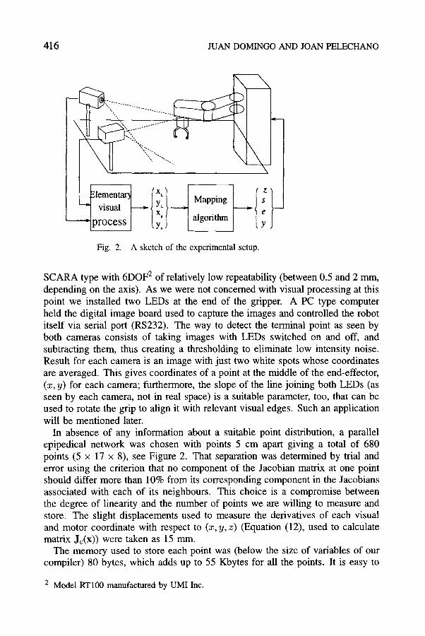
Fig. 2. A sketch of the experimental setup.

SCARA type with 6DOF 2 of relatively low repeatability (between 0.5 and 2 mm, depending on the axis). As we were not concerned with visual processing at this point we installed two LEDs at the end of the gripper. A PC type computer held the digital image board used to capture the images and controlled the robot itself via serial port (RS232). The way to detect the terminal point as seen by both cameras consists of taking images with LEDs switched on and off, and subtracting them, thus creating a thresholding to eliminate low intensity noise. Result for each camera is an image with just two white spots whose coordinates are averaged. This gives coordinates of a point at the middle of the end-effector, (x, y) for each camera; furthermore, the slope of the line joining both LEDs (as seen by each camera, not in real space) is a suitable parameter, too, that can be used to rotate the grip to align it with relevant visual edges. Such an application will be mentioned later.

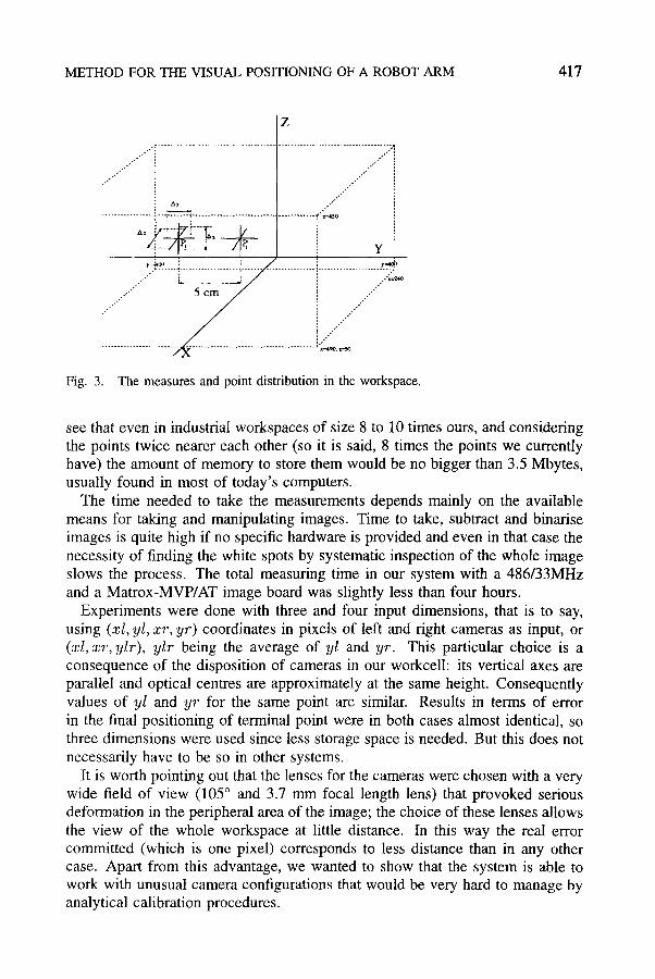
In absence of any information about a suitable point distribution, a parallel epipedical network was chosen with points 5 cm apart giving a total of 680 points (5 x 17 x 8), see Figure 2. That separation was determined by trial and error using the criterion that no component of the Jacobian matrix at one point should differ more than 10% from its corresponding component in the Jacobians associated with each of its neighbours. This choice is a compromise between the degree of linearity and the number of points we are willing to measure and store. The slight displacements used to measure the derivatives of each visual and motor coordinate with respect to (x, y, z) (Equation (12), used to calculate matrix Jc(x)) were taken as 15 mm.

The memory used to store each point was (below the size of variables of our compiler) 80 bytes, which adds up to 55 Kbytes for all the points. It is easy to

2 Model RT100 manufactured by UMI Inc.


Z

...... ........ i . . . . . . . . . . . . . . . . . . . . . . . . . . . . . . . . . . . . . . . . . . . . . . . . ..'"

. . . . . . . . . . . . . . . . . ~ - - - . . . . . . ~ . . . . . . . . . . . . . . . . . . . . . . . . . . . . . . . . . . . . . . . ~ ~ - ~ o

~ Y y : ~ , , i . . j : 7=~'.

., .,"�9 ,-, i~ 5c~ ~ i ,-',--~ / /

/ r x - - - x --.,1~o, ~'-~0

Fig. 3. The measures and point distribution in the workspace.

see that even in industrial workspaces of size 8 to 10 times ours, and considering the points twice nearer each other (so it is said, 8 times the points we currently have) the amount of memory to store them would be no bigger than 3.5 Mbytes, usually found in most of today's computers.

The time needed to take the measurements depends mainly on the available means for taking and manipulating images. Time to take, subtract and binarise images is quite high if no specific hardware is provided and even in that case the necessity of finding the white spots by systematic inspection of the whole image slows the process. The total measuring time in our system with a 486/33MHz and a Matrox-MVP/AT image board was slightly less than four hours.

Experiments were done with three and four input dimensions, that is to say, using (:r/, yt, xr, yr) coordinates in pixels of left and right cameras as input, or (x/, zr, ylr), ylr being the average of yl and yr. This particular choice is a consequence of the disposition of cameras in our workcell: its vertical axes are parallel and optical centres are approximately at the same height. Consequently values of yl and yr for the same point are similar. Results in terms of error in the final positioning of terminal point were in both cases almost identical, so three dimensions were used since less storage space is needed. But this does not necessarily have to be so in other systems.

It is worth pointing out that the lenses for the cameras were chosen with a very wide field of view (105 ~ and 3.7 mm focal length lens) that provoked serious deformation in the peripheral area of the image; the choice of these lenses allows the view of the whole workspace at little distance. In this way the real error committed (which is one pixel) corresponds to less distance than in any other case. Apart from this advantage, we wanted to show that the system is able to work with unusual camera configurations that would be very hard to manage by analytical calibration procedures.


5. R e s u l t s

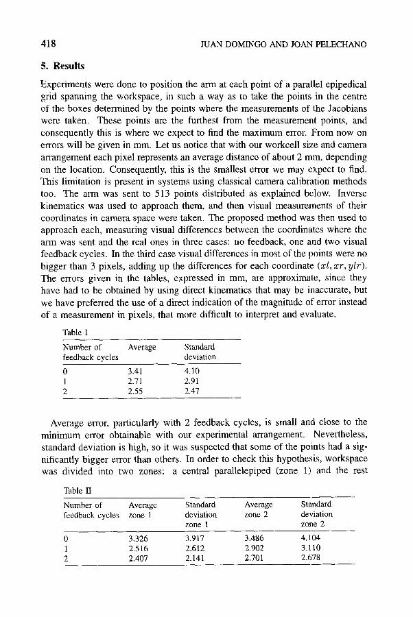
Experiments were done to position the arm at each point of a parallel epipedical grid spanning the workspace, in such a way as to take the points in the centre of the boxes determined by the points where the measurements of the Jacobians were taken. These points are the furthest from the measurement points, and consequently this is where we expect to find the maximum error. From now on errors will be given in mm. Let us notice that with our workcell size and camera arrangement each pixel represents an average distance of about 2 ram, depending on the location. Consequently, this is the smallest error we may expect to find. This limitation is present in systems using classical camera calibration methods too. The ann was sent to 513 points distributed as explained below. Inverse kinematics was used to approach them, and then visual measurements of their coordinates in camera space were taken. The proposed method was then used to approach each, measuring visual differences between the coordinates where the arm was sent and the real ones in three cases: no feedback, one and two visual feedback cycles. In the third case visual differences in most of the points were no bigger than 3 pixels, adding up the differences for each coordinate (xl, xr, ylr). The errors given in the tables, expressed in mm, are approximate, since they have had to be obtained by using direct kinematics that may be inaccurate, but we have preferred the use of a direct indication of the magnitude of error instead of a measurement in pixels, that more difficult to interpret and evaluate.

Table I

Number of A v e r a g e Standard feedback cycles deviation

0 3.41 4.10 1 2.71 2.91 2 2.55 2.47

Average error, particularly with 2 feedback cycles, is small and close to the minimum error obtainable with our experimental arrangement. Nevertheless, standard deviation is high, so it was suspected that some of the points had a sig- nificantly bigger error than others. In order to check this hypothesis, workspace was divided into two zones: a central parallelepiped (zone 1) and the rest

Table II

Number of A v e r a g e Standard Average Standard feedback cycles zone 1 deviation zone 2 deviation

zone 1 zone 2

0 3.326 3.917 3.486 4.104 1 2.516 2.612 2.902 3.110 2 2.407 2.141 2.701 2.678


(zone 2), each one containing half of the test points. The results are shown in Table II.

As it is seen, errors are always bigger in the outer part of the workspace. The reason for this behaviour is that real size of the space area captured by a single pixel is bigger in peripheral areas due to the lens distortion. Experiments of this type may be used as a guide to determine in which areas new measurements may be needed if the number of feedback cycles is excessive.

Another experiment consisted of misaligning the cameras intentionally by an unknown amount with a slight touch. In this way all the visual measurements are affected by some error and the associated Jacobian is not that measured for the corresponding real point but for a close point. This is equivalent to operating with a point whose distance to the nearest measured neighbour is the original, plus the camera misalignment. The consequence is that more feedback cycles are needed to obtain the same precision, but the arm still goes to the point where cameras want to see it. The number of feedback cycles was no bigger than 5 in any of the 25 points where this was checked to reach the desired visual point with a total error no bigger than 3 pixels. The camera misalignment in this case was no bigger than approximately 10 ~ in each axis (yaw and pitch).

The third experiment was a practical task: the building of a tower of blocks using entirely visual information (no cartesian coordinates for the initial positions and orientations of the blocks are known). As we are only concerned with control aspects, the visual process was simplified as much as possible by using white blocks on a black background with no overlapping allowed. The localisation is then simply done by thresholding with a fixed value. Blocks are treated as visual blobs, whose vertical axis is determined by specific methods (moments or simply centre of convex hull). The visual point to which the arm is to be sent has horizontal coordinate on the axis and vertical coordinate up to the superior limit of the block. In more complex shaped blocks it might be necessary to position the arm more precisely up to the block. In such a case visual metric tensors can be used to transform pixels in real distances at that area of the image. The localized terminal point of the arm placed at the desired place is shown in Figure 4.

Fig. 4. Arm ready to pick one block as seen by left and right cameras.


Fig. 5. Cylinder visually centered on prism.

Fig. 6. The final tower built.

The next step before going down and closing gripper to grasp block is to orient the hand. This was done visually, too, by rotating it until the line joining both LEDs is seen by both cameras parallel to line A-B (that is to say, their slopes in the image planes are equal). Determination of line A-B was done in our case by polygonal fitting of the visual blob.

Picking of other blocks is done in the same way, and placing on the top of the former is achieved by getting the superior blob visually centered with respect to the one below it. An intermediate step is shown at Figure 5. Figure 6 depicts the final tower.

Although simple, the main purpose of this experiment was to show that as- semblies can be built through the detection and use of relevant visual features without making explicit reference to Cartesian positions or orientations.

6. Conclusions and future work

We have shown how a local linear approximation obtained through the measurement and storage of a set of Jacobians can be considered a good method to position a robot arm where a pair of non-calibrated cameras want to see


it, and that the measurement time and storage space are into the limits of the current industrial and experimental systems. The feedback capacity makes the system precise enough when reaching a point, apart from being able to cope with little disturbances of the environment. Differently from former approaches, Jacobian matrices are not calculated from previous knowledge on the geometry of the system or the optical system or arrangement of the cameras. Apart from that, having Jacobians stored, instead of calculating them on line, as in common practice, may accelerate the calculations for positioning and permit a real time implementation at a little computational cost; nevertheless, detection of relevant visual features would have to be done with real time visual specific hardware whose unavailability has deprived us a real time implementation. The conclusion is that the method can be applied to simple industrial environments where parts arrive at random positions and orientations as long as a visual system is able to detect some of their relevant features like vertices or edges. Such detection is an important topic of research, see for instance (Bien et al., 1993).

Further work will include the possibility of using the method with orientable cameras. The mapping would be established between visual position of the tip of the arm and orientation angles for the platform of each camera, the objective being the vision of the terminal point at the centre of the image; at this moment the algorithm described hereafter with static cameras would be applied. This would allow the use of lenses with small field of view thus decreasing the absolute error at a given resolution. The optimal placement of sensors have been addressed by Nelson and Khosla (1994). Furthermore, it would be a way to simulate the usual two phase behaviour of humans that execute saccadic movements to follow hands plus eye fixation when assembling objects.

References

Amillo and Arriaga: 1986, Andlisis Mathemdtico con Aplicaciones a la Computaci6n, McGraw-Hill.

Albus, S. J.: 1981, A neurological model, in Brains, Behaviour and Robotics, BYTE Books, McGraw-Hill.

Atkeson, C. G.: April 1991, Using locally weighted regression for robot learning, in Proc. IEEE Int. Conf. on Robotics and Automation, Sacramento, CA, IEEE Computer Society Press, pp. 958-963.

Bien, Z., Jang, W., and Park, J.: 1993, Characterization and use of feature-Jacobian matrix for visual servoing, in Visual Servoing, World Scientific, pp. 317-363.

Bentley, J. L. and Papadimitriou, C. H.: April 1980, Two papers on computational geometry, Tech. Report CMU-CS-80-109, Dept. of Computer Science, Carnegie-Mellon University.

Conkie, A. and Chongstitvatana, P.: 1990, An uncalibrated stereo visual servo system, in Proc. British Machine Vision Conf., Oxford, pp. 277-280.

Corke, P. I.: 1993, Visual control of robot manipulators, in Visual Servoing, A Review, World Scientific, pp. 1-31.

Domingo, J.: September 1991, Stereo part mating, Master's Thesis, Department of Artificial Intelligence, Univ. of Edinburgh.


Domingo, J.: November 1993, lmplantaci6n y Comparacidn de diversos Mgtodos para Con- trol de Robot basados en Visi6n, PhD Thesis, Departamento de Inform~itica y Electr6nica, Univ. de Valencia.

Feddema, J. T., Lee, C. S. G., and Mitchell, O. R.: 1993, Feature-based visual servoing of robotic systems, in Visual Servoing, World Scientific, pp. 105-138.

Hashimoto, K. and Kimura, H.: 1993, LQ optimal and nonlinear approaches to visual servoing, in Visual Servoing, World Scientific, pp. 139-164.

Krose, J. A., van der Smagt, P. P., and Groen, E C. A.: 1993, One eyed self learning robot manipulator, in Bekey et al. (eds), Neural Networks in Robotics, Kluwer Academic Publishers, pp. 19-27.

Miller, W. T., Glanz, E H., and Kraft, L. G.: 1990, Real-time dynamic control of an industrial manipulator using a neural-network-based leaming controller, in IEEE Trans. Robotics and Automation 6(1), 1-9.

Nelson, B. J. and Khosla, P. K.: 1994, The resolvability ellipsoid for visual servoing, in Proc. Vision and Pattern Recognition CVPR94, Washington, DC.

Nelson, B., Papanikopoulos, N. P., and Khosla, P. K.: 1993, Visual servoing for robotic assembly, in Visual Servoing, World Scientific, pp. 139-164.

Pellionisz, A.: 1985, Tensorial aspects of the multidimensional approach to the vestibulo- oculomotor reflex and gaze, in Berthod and Melvill Jones (eds), Adaptive Mechanisms in Gaze Control.

Pellionisz, A. and Llin~is, R.: 1980, Tensorial approach to the geometry of the brain function: Cerebellar coordination via a metric tensor, Neuroscience S, 1125-1136.

Tsai, R. Y.: 1987, A versatile camera calibration technique for high accuracy 3d machine vision metrology using off-the-shelf tv cameras and lenses, in IEEE Trans. Robotics and Automation 3, 323-344.

Measurement and storage of a network of jacobians as a method for the visual positioning of a robot...

Documents

Transcript of Measurement and storage of a network of jacobians as a method for the visual positioning of a robot...