Measured crest height distribution compared to second ... · Measured crest height distribution...

Measured crest height distribution compared to second order distribution

14th International Workshop on Wave Hindcasting and Forecasting.

Key West, Florida, USA, Nov 8-13, 2015

ABSTRACT

When designing and verifying the structural integrity of an installation the loads that can affect the

structure need to be determined. For the Norwegian continental shelf the governing regulations is given by

the Petroleum Safety Authority. It states that the loads/actions that can affect the facilities shall be

determined. Further, it states that accidental actions and metocean actions with an annual probability of 10-4

or greater shall not result in loss of main safety functions.

In principle a full long term analysis is required in order to obtain consistent estimates for the metocean

actions. This is straight forward for linear response problems, while it is a challenge for non-linear problems

in particular if they additionally are of an on-off nature. The latter will typically be the case for loads due to

wave in deck and breaking wave impacts.

In this paper, the second order distribution by Forristall will be discussed and compared to

measurements(2004-2015) from a North Sea location at 190 m water depth. Long term analyses of crest

height using short crested versus long crested waves will be discussed.

Measured crest height distribution compared

to second order distribution

Gunnar Lian Statoil / University of Stavanger

Stavanger, Norway

Sverre K Haver University of Stavanger

Stavanger, Norway


2

I. INTRODUCTION

hen designing a fixed drag dominated structure for

wave loading a common approach is to use the so called

“design wave approach”. This is normally specified by

a long crested Stokes 5th

order wave. The wave height with

annual probability of 10-2

is used for Ultimate Limit State

(ULS). For Accidental Limit State (ALS) annual probability

of exceedance of 10-4

is used. The worst wave period within a

90 percent confidence interval is used, normally in the range

+/- 2 s. If the structure responds dynamically to the wave

loading, this has to be taken into account by adding the inertia

load as an acceleration field. A structure is normally

considered to respond dynamically to wave loading when the

natural period of the structure is above 3 second.

In addition to the general wave loading, the airgap of

installation has to be checked. If the extreme wave crest hits

the deck. The solution will be to increase the air gap for new

installations. For an existing installation the structural capacity

has to be verified.

Thus the crest height with an appropriate annual probability

has to be estimated. It should be noted that this crest will be

higher than the crest given by the Stokes 5th

design wave used

in the design wave approach.

A common approach to estimate the extreme wave crest,

used widely for the Norwegian continental shelf, is to perform

a long term analysis utilizing the all sea state approach in

combination with the short term second order distribution

given by Forristall [1]

The crest distribution is a function of the wave steepness

and the water depth. When the waves become very steep the

crest height is limited by breaking. Extensive testing in model

basin has been performed and there is an indication of

increased crest heights beyond the second order crest even in

directional spread sea, [2], [3], [4].

II. SECOND ORDER WAVE CREST DISTRIBUTION

The sea surface elevation is now commonly described by a

second order process. Based on second order time domain

simulations, Forristall, [1] established a short term distribution

of the crest heights. Key features of the numerical simulations

performed by Forristall are:

- JONSWAP spectra.

- Peak enhancement factor 3.3(some 1.0 and 10).

- Water depths 10, 20, 40 m, and infinite.

- Peak periods 8, 10 and 12 s.

- Steepness Sp 0.01 to 0.1, in steps of 0.01

- Simulation length 1024s, repeated 10 000 times.

- Long crested and short crested using Ewans

spreading function for fetch limited sea,[5].

This distribution is commonly used to estimate the long

term estimate of the extreme crests. The short term

distribution is given by the following 2 parameters Weibull

distribution:

( ) [ (

)

] (1)

Forristall fitted the Weibull location and scale parameter as

a function of the water depth(Ursell number) and the wave

steepness. He found that using the mean wave period( ),

rather than the peak period produced a better fit for spectra

with same peak period but different peak enhancement factors.

The steepness parameter is then given by:

(2)

Where is the mean wave period estimated from the two

first moment of the wave spectrum , ⁄ .

The effect of water depth is described by the Ursell number.

(3)

Where is the finite depth wavenumber for a frequency of

⁄ Note that the steepness is estimated using infinite water

depth, but the wave number is estimated for finite water depth.

The estimated parameters are forced to match the Rayleigh

distribution with √ ⁄ and at zero steepness and

Ursell number.

For long crested seas the Weibull parameters are given by:

(4)

(5)

For short crested seas the Weibull parameters are given by:

(6)

(7)

A stationary sea state of 3-hour duration is often considered.

The 3-hour extreme crest distribution can then be estimated

from:

( ) ( [ (

)

])

(8)

Where is the expected number of global crests in 3-

hour. A global crest is largest crest between zero-up crossings.

The p-fractile for 3-hour can then be estimated from

[ ( ( ) )]

(9)

The long term extreme crest should be estimated using a

long term analysis. Alternatively, it can be estimated using the

contour line method. The sea state at the peak of the contour

and a fractile of 85%-90% for ULS and 90%-95% for ALS

should then be used.

W


3

A. Sensitivity to steepness and water depth

For jacket structures in the North Sea we are mainly

interested in water depths of 80-190m, but to investigate the

sensitivity to water depth and steepness a sensitivity analysis

of the following cases is investigated. : Water depth from 80

to 1000 m. and Hs 18 m. Steepness varying from

0.01 to 0.1.

Steepness Sp is defined by

(10)

Contours of constant probability of exceedance (q) can be

constructed for Hs and Tp. In deep water when the Ursell

number approaches 0, the crest distributions will be the same

in sea states that have the same steepness. Figure 1 show an

example of contour lines and the steepness varying from 0.01

to 0.1. The green solid lines in Figure 1 indicate the area

< √ ⁄ < , where it is expected that the JONSWAP

spectrum is a reasonable model according to [6]. This

corresponds to steepness between 0.025 and 0.05. From the

contour diagram we see that the highest steepness of 0.1 will

only occur in low sea states. The peak of the contour is

between 0.030-0.040.

Figure 1 Example of contour lines of Hs and Tp with the steepness Sp shown as dashed lines.

In this sensitivity analysis it is assumed that the JONSWAP

spectrum is a representative model.

The mean wave period and the zero upcrossing period is

estimated by the following relations taken from [6].

(

) (11)

(

) (12)

The number of global wave crests is then estimated by

(13)

The JONSWAP peak enhancement factor is estimated by

the relation given by [7]

[ ] (14)

The wave length is estimated by the following equation

from [6].

√ √ ( )

( )

where ( ) ∑ , ( ) ( )⁄

and , , , .

(15)

The target probability level for the characteristic value is

varying for different sea states, since the number of crests is

varying. The exceedance probability for the characteristic

largest crest in 3-hour is ⁄ , where is the expected

number of crests during 3-hour. The characteristic largest crest

is then given by:

[ (

)]

(16)

The characteristic largest crest height during 3-hour is

estimated for sea states indicated by green circles in Figure 1

for 5 different water depths. The is normalized by the

significant wave height and shown in Figure 2 as a function of

steepness.

From the figure we see that for water depth deeper than

100m that the Ursell number has little impact on the crest

distribution compared to the steepness. It is also noted that the

normalized characteristic largest crest increase with increasing

steepness.

Figure 2 ⁄ as a function of steepness for different water depths. Long crested waves.


4

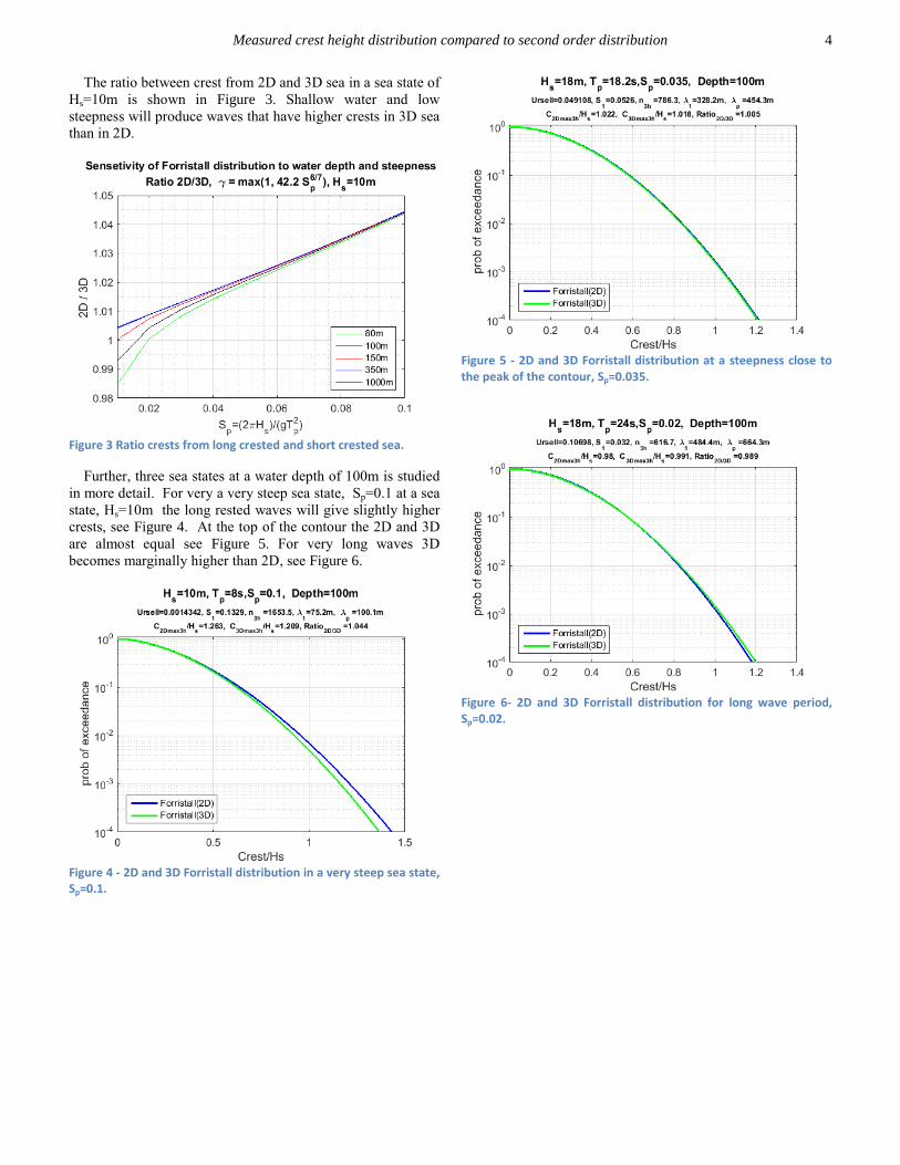
The ratio between crest from 2D and 3D sea in a sea state of

Hs=10m is shown in Figure 3. Shallow water and low

steepness will produce waves that have higher crests in 3D sea

than in 2D.

Figure 3 Ratio crests from long crested and short crested sea.

Further, three sea states at a water depth of 100m is studied

in more detail. For very a very steep sea state, Sp=0.1 at a sea

state, Hs=10m the long rested waves will give slightly higher

crests, see Figure 4. At the top of the contour the 2D and 3D

are almost equal see Figure 5. For very long waves 3D

becomes marginally higher than 2D, see Figure 6.

Figure 4 - 2D and 3D Forristall distribution in a very steep sea state, Sp=0.1.

Figure 5 - 2D and 3D Forristall distribution at a steepness close to the peak of the contour, Sp=0.035.

Figure 6- 2D and 3D Forristall distribution for long wave period, Sp=0.02.


5

III. FULL SCALE MEASSUREMENTS

The measurement is performed by a wave radar type

WaveRadar REX manufactured by SABB/Rosemount. The

microwave beam has a 10 degree wide cone. The sampling

frequency is 7.68Hz. A comprehensive review of wave radar

measurements can be found in [8], [9].

Each time series has a length of 20 minutes. The mean is

subtracted from each time series. Obviously erroneous time

series has been removed.

The full scale measurement has been performed since 2004.

There has been some down time, so the total available time

series are 132752 x 20 min = 44250 hours. Of those

6348x20min = 2116 hours are in sea states above Hs 6.5m, and

183x20min = 61 hours above Hs 10.5m.

The highest measured 20 min. sea state is Hs=14.1m. The

maximum crest in this sea state was 12.0m. The highest

measured crest was 15.1m. This was in a sea state of

Hs=12.1m.

A total of 2028 hours of measured surface elevation has

been compared to the Forristall second order crest distribution.

The comparison has in general been limited to sea state class

with minimum 10 hours of observations. The measurements

are binned into blocks of one meter and one second. Steepness

from 0.018 to 0.055 are covered, as indicated by the shaded

area in Table 1. The number of hours of measurements in each

block is given in Table 2.The selected sea states are shown

along with the contour lines in Figure 7.

Table 1 Steepness for the measured sea states are shown in shaded area.

Tp[s]

Hs

[m]

9 10 11 12 13 14 15 16 17 18

7 0.055 0.045 0.037 0.031 0.027 0.023 0.020 0.018 0.016 0.014

8 0.063 0.051 0.042 0.036 0.030 0.026 0.023 0.020 0.018 0.016

9 0.071 0.058 0.048 0.040 0.034 0.029 0.026 0.023 0.020 0.018

10 0.079 0.064 0.053 0.045 0.038 0.033 0.028 0.025 0.022 0.020

11 0.087 0.071 0.058 0.049 0.042 0.036 0.031 0.028 0.024 0.022

Table 2 Total hours of measurement of each sea state class.

Tp[s]

Hs

[m]

9 10 11 12 13 14 15 16 17 18

7 41.7 187.0 374.7 281.7 130.7 83.7 53.3 32.0 29.0 18.0

8

32.3 149.7 175.3 57.0 33.0 17 13.3 16.7

9

27.7 61.7 58.3 25.3 13.3

10

23.7 37.0 27.3

11 13.7 14.0

Figure 7 Sea states used for comparison with second order and full scale measurements.

In addition to comparing the visual plot of the measurement

and second order distribution, the characteristic largest in a 3-

hour sea states is compared.

The Gumbel extreme distribution is used to estimate the

distribution of the largest:

( ) { [ (

)]} (17)

Where is the scale parameter and the location

parameter, [10].

The 3-hour mean and variance is given by:

( ) (18)

(19)

The location and scale parameters is estimated by the

methods of moment (MOM), by solving equation (18) and

(19).

There are several ways of estimating the characteristic

largest in 3-hour from the measured 20minutes time series.

One could for example randomly merge 9 time series and

establish the Gumbel distribution of the largest. The

characteristic largest can then be estimated by the most

probably maximum (mpm) i.e the 37% fractile. This can be

repeated several times and averaged.

We have chosen to establish the Gumbel distribution

directly for the maximum in each 20 minutes series, the 3-hour

distribution is then given by:


6

( ) { ( )} (20)

The characteristic largest in 3-hour can then be estimated by

the mpm of the Gumbel distribution, i.e the 37th

percentile.

( ( ))

(21)

This is compared to the characteristic largest estimated from

the Forristall 3D distribution. To be consistent, we use the

Gumbel extreme distribution instead of the true extreme

distribution. For the 3-hour fractiles in the range of 37%-57%

they give similar crests in this case. The deviation becomes

larger further out in the tail. We estimate the Gumbel

parameter from the asymptote of the largest observation from

a Weibull distribution given by [10].

( ( ))

(22)

( ( ))

(23)

Where and are the Weibull scale and shape

parameter respectively. n is the number of global crests in 3-

hour. This can either be counted from the time series, or

estimated by assuming JONSWAP spectra and equation (13).

We have chosen the latter, in this comparison. The

characteristic largest from second order distribution is then

estimated by:

( ( )) (24)

A. Results

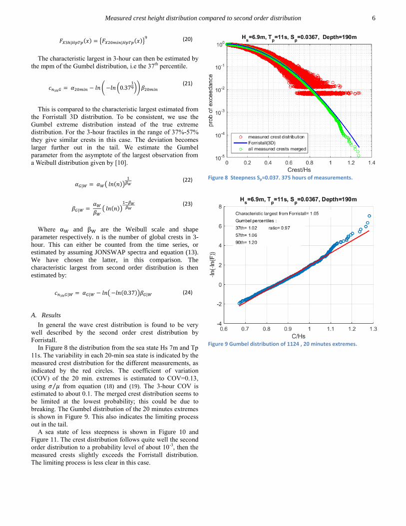
In general the wave crest distribution is found to be very

well described by the second order crest distribution by

Forristall.

In Figure 8 the distribution from the sea state Hs 7m and Tp

11s. The variability in each 20-min sea state is indicated by the

measured crest distribution for the different measurements, as

indicated by the red circles. The coefficient of variation

(COV) of the 20 min. extremes is estimated to COV=0.13,

using ⁄ from equation (18) and (19). The 3-hour COV is

estimated to about 0.1. The merged crest distribution seems to

be limited at the lowest probability; this could be due to

breaking. The Gumbel distribution of the 20 minutes extremes

is shown in Figure 9. This also indicates the limiting process

out in the tail.

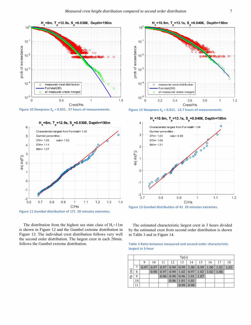
A sea state of less steepness is shown in Figure 10 and

Figure 11. The crest distribution follows quite well the second

order distribution to a probability level of about 10-3

, then the

measured crests slightly exceeds the Forristall distribution.

The limiting process is less clear in this case.

Figure 8 Steepness Sp=0.037. 375 hours of measurements.

Figure 9 Gumbel distribution of 1124 , 20 minutes extremes.


7

Figure 10 Steepness Sp = 0.031. 57 hours of measurements.

Figure 11 Gumbel distribution of 171 20 minutes extremes.

The distribution from the highest sea state class of Hs=11m

is shown in Figure 12 and the Gumbel extreme distribution in

Figure 13. The individual crest distribution follows very well

the second order distribution. The largest crest in each 20min.

follows the Gumbel extreme distribution.

Figure 12 Steepness Sp = 0.011. 13.7 hours of measurements.

Figure 13 Gumbel distribution of 41 20 minutes extremes.

The estimated characteristic largest crest in 3 hours divided

by the estimated crest from second order distribution is shown

in Table 3 and in Figure 14.

Table 3 Ratio between measured and second order characteristic largest in 3-hour

Tp[s]

Hs

[m]

9 10 11 12 13 14 15 16 17 18

7 0.97 0.97 0.97 0.99 0.99 1.00 0.99 1.00 1.02 1.03

8 0.98 0.97 0.99 1.02 0.97 1.02 1.02 1.06

9 0.96 0.98 0.96 1.01 1.07

10 0.96 1.01 1.01

11 0.99 0.98


8

A special storm the 26th

of January 2012 lasting for more

than 24 hours gave significantly higher crest distribution than

second order, as shown by the red dot in Figure 14. The crest

distribution is shown in Figure 15. For another data set, a

similar significant deviation from the second order distribution

is described in [11].

From Figure 14 there is a slope from the least steep towards

the steep waves. This is somewhat linked to the number of

waves. For the longest wave period there is a larger number up

crossings than estimated using JONSWAP spectra, and for the

shortest period, slightly smaller number than estimated. If the

counted crests are used when estimating the characteristic

largest crest from second order, instead of the estimated, the

blue squares in Figure 14 will be slightly more level, but with

the same tendency. The green squares indicate the change

when using counted crests versus estimated at that steepness.

For the sea state class where the highest blue square is

measured there is only 13.3 hour of measuring, and the next

highest only 16.7 hours.

Figure 14 Ratio between measured and second order characteristic largest in 3-hour.

Figure 15 Crest Distribution 26 of January 2012. The characteristic largest is 7% higher than estimated by second order.

The time serie during the 26th

of January 2012 is shown in

Figure 16. The storm is almost constant at a significant wave

height of 11m for 24 hour. The Gumbel extreme value

distribution of the 20 minutes extremes are shown in Figure

17. The characteristic largest crest during 3-hour is estimated

to 7% higher than estimated from second order distribution.

Figure 16 measured metocean condition during the 26

th of January

2012.


9

Figure 17 Gumbel plot of 20 min extremes. The percentiles are adjusted to 3hour extremes.

Each of the eight 3-hour distributions during the 26th of

January 2012 are shown in Figure 18. It shows that for most of

the 3-hour periods, the crests exceed the second order

distribution.

Figure 18 Each 3-hour crest distribution 26 of January 2012

The largest crest in the measuring period is 15m. This crest

was measured in the evening of the 12th

of January 2015. The

crest distribution is shown in Figure 19. The time series

around the extreme crest is shown in Figure 20, and the

estimated wave spectra in Figure 21.

Figure 19 Crest distribution 12

th january 2012 from 1800-2100

Figure 20 Exteme crest of 15 meter in sea state of Hs= 12m


10

Figure 21 Wave spectra 12

th january 2012 from 18:00-21:00.

IV. LONG TERM ANALYSIS USING ALL SEA APPROACH

We will now discuss long term analysis using all seas

approach based on hindcast. When a long term analysis is

performed using all seas approach, both the long – and short

term inherent randomness is considered, Haver [12]. By

considering the joint distribution fHsTp(hs,tp), of the significant

wave height, Hs, and the spectral peak period Tp, the long term

inherent randomness of the sea state severity is taken into

account. A stationary sea state of 3hours duration is

considered in the present work. The inherent randomness for

the extreme response value in the 3-hour sea state is given by

the short term conditional extreme value distribution FX3h |

HsTp(x|hs,tp,).

The long term analysis (LTA) can be done by considering

the 3-hour maximum as the target response quantity.

The long term distribution of X3h is given by:

( ) ∬ ( | )

( )

(25)

The target annual exceedance probability q is then given by:

( ) (26)

is the annual number of events in the target population,

if all 3-hours event in a year is included the target population

is 2920. It is then assumed that all 3 hours extremes are

statistically independent. This is not the case, and the

estimated extreme value is expected to be slightly on the safe

side. The short term distribution function of X3h must be in

agreement with the underlying physics of the response

problem. The physics of the problem is related to the

distribution of X3h.

The long term description of the sea state can be estimated

by fitting probability functions to the hindcast data.

The joint probability density function is given for Hs and Tp

according to the following equation:

( ) ( ) ( ) (27)

The long term distribution of the significant wave height is

modeled by a 3 parameter Weibull distribution:

( ) ( (

)

) (28)

The significant wave for a given annual probability of

exceedance can be estimated by

( ) ( (

))

(29)

The probability density function for is found by

derivation of (28) :

( )

(

)

( (

)

) (30)

Conditional distribution for Tp given Hs:

( )

√ (

( ( ) )

)

(31)

where [ ] and [ ] given by:

(32)

( ) (33)

Table 4: Parameters in the annual omni-directional joint distribution for Hs and Tp .

(shape) ( ) ( )

1.345 2.20 0.53

1.653 0.397 0.395 0.005 0.096 0.283

When estimating long term crest height using all sea state

approach and Forristall crest distribution, the long term

distribution of the 3-hour maximum crest height is given by:

( ) ∬{ ( )}

( ) (34)

is the zero up crossings period. By assuming JONSWAP

spectrum is estimated by equation (12)

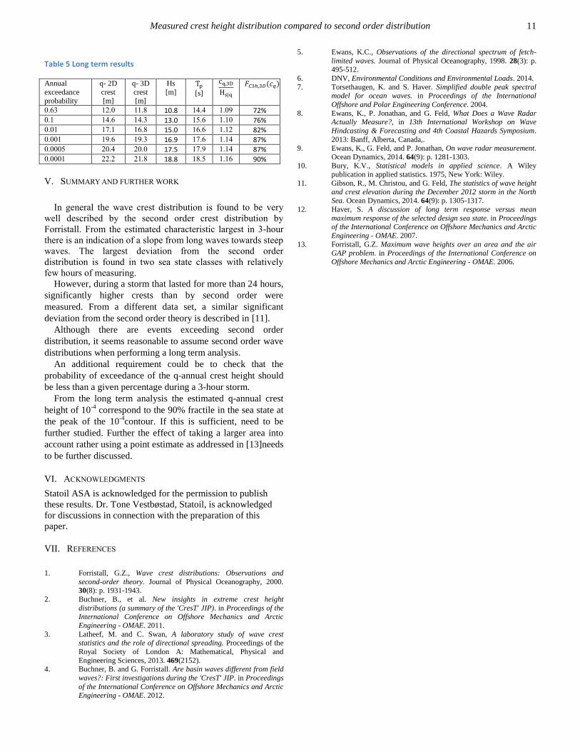
From the long term analysis we can see in Table 5 (column

2 and 3) that there is relatively little difference between the

crest heights using 2D or 3D distribution. In column 6 the q-

annual crest estimated by 3D distribution is normalized by the

q-annual significant wave height. In column 7 the fractiles for

the q-annual 3D crest is given.


11

Table 5 Long term results

Annual

exceedance probability

q- 2D

crest [m]

q- 3D

crest [m]

Hs

[m]

[s]

( )

0.63 12.0 11.8 10.8 14.4 1.09 72% 0.1 14.6 14.3 13.0 15.6 1.10 76% 0.01 17.1 16.8 15.0 16.6 1.12 82% 0.001 19.6 19.3 16.9 17.6 1.14 87% 0.0005 20.4 20.0 17.5 17.9 1.14 87% 0.0001 22.2 21.8 18.8 18.5 1.16 90%

V. SUMMARY AND FURTHER WORK

In general the wave crest distribution is found to be very

well described by the second order crest distribution by

Forristall. From the estimated characteristic largest in 3-hour

there is an indication of a slope from long waves towards steep

waves. The largest deviation from the second order

distribution is found in two sea state classes with relatively

few hours of measuring.

However, during a storm that lasted for more than 24 hours,

significantly higher crests than by second order were

measured. From a different data set, a similar significant

deviation from the second order theory is described in [11].

Although there are events exceeding second order

distribution, it seems reasonable to assume second order wave

distributions when performing a long term analysis.

An additional requirement could be to check that the

probability of exceedance of the q-annual crest height should

be less than a given percentage during a 3-hour storm.

From the long term analysis the estimated q-annual crest

height of 10-4

correspond to the 90% fractile in the sea state at

the peak of the 10-4

contour. If this is sufficient, need to be

further studied. Further the effect of taking a larger area into

account rather using a point estimate as addressed in [13]needs

to be further discussed.

VI. ACKNOWLEDGMENTS

Statoil ASA is acknowledged for the permission to publish

these results. Dr. Tone Vestbøstad, Statoil, is acknowledged

for discussions in connection with the preparation of this

paper.

VII. REFERENCES

1. Forristall, G.Z., Wave crest distributions: Observations and

second-order theory. Journal of Physical Oceanography, 2000. 30(8): p. 1931-1943.

2. Buchner, B., et al. New insights in extreme crest height

distributions (a summary of the 'CresT' JIP). in Proceedings of the International Conference on Offshore Mechanics and Arctic

Engineering - OMAE. 2011.

3. Latheef, M. and C. Swan, A laboratory study of wave crest statistics and the role of directional spreading. Proceedings of the

Royal Society of London A: Mathematical, Physical and

Engineering Sciences, 2013. 469(2152). 4. Buchner, B. and G. Forristall. Are basin waves different from field

waves?: First investigations during the 'CresT' JIP. in Proceedings

of the International Conference on Offshore Mechanics and Arctic Engineering - OMAE. 2012.

5. Ewans, K.C., Observations of the directional spectrum of fetch-

limited waves. Journal of Physical Oceanography, 1998. 28(3): p. 495-512.

6. DNV, Environmental Conditions and Environmental Loads. 2014.

7. Torsethaugen, K. and S. Haver. Simplified double peak spectral model for ocean waves. in Proceedings of the International

Offshore and Polar Engineering Conference. 2004.

8. Ewans, K., P. Jonathan, and G. Feld, What Does a Wave Radar Actually Measure?, in 13th International Workshop on Wave

Hindcasting & Forecasting and 4th Coastal Hazards Symposium.

2013: Banff, Alberta, Canada,. 9. Ewans, K., G. Feld, and P. Jonathan, On wave radar measurement.

Ocean Dynamics, 2014. 64(9): p. 1281-1303.

10. Bury, K.V., Statistical models in applied science. A Wiley publication in applied statistics. 1975, New York: Wiley.

11. Gibson, R., M. Christou, and G. Feld, The statistics of wave height

and crest elevation during the December 2012 storm in the North Sea. Ocean Dynamics, 2014. 64(9): p. 1305-1317.

12. Haver, S. A discussion of long term response versus mean

maximum response of the selected design sea state. in Proceedings of the International Conference on Offshore Mechanics and Arctic

Engineering - OMAE. 2007.

13. Forristall, G.Z. Maximum wave heights over an area and the air

GAP problem. in Proceedings of the International Conference on

Offshore Mechanics and Arctic Engineering - OMAE. 2006.

Measured crest height distribution compared to second ... · Measured crest height distribution...

Documents

Transcript of Measured crest height distribution compared to second ... · Measured crest height distribution...