Mean-Variance Analysis · 2017-01-26 · Mean-variance analysis 1/ 51. 2.1: Assumptions 2.2:...
51
2.1: Assumptions 2.2: Indi/erence 2.3: Frontier 2.4: R f 2.5: Hedging 2.6: Summary Mean-Variance Analysis George Pennacchi University of Illinois George Pennacchi University of Illinois Mean-variance analysis 1/ 51
-
Upload
nguyendang -
Category
Documents
-
view
233 -
download
1
Transcript of Mean-Variance Analysis · 2017-01-26 · Mean-variance analysis 1/ 51. 2.1: Assumptions 2.2:...

2.1: Assumptions 2.2: Indi¤erence 2.3: Frontier 2.4: Rf 2.5: Hedging 2.6: Summary
Mean-Variance Analysis
George Pennacchi
University of Illinois
George Pennacchi University of Illinois
Mean-variance analysis 1/ 51

2.1: Assumptions 2.2: Indi¤erence 2.3: Frontier 2.4: Rf 2.5: Hedging 2.6: Summary
Introduction
How does one optimally choose among multiple risky assets?
Due to diversi�cation, which depends on assets�returncovariances, the attractiveness of an asset when held in aportfolio may di¤er from its appeal when it is the sole assetheld by an investor.
Hence, the variance and higher moments of a portfolio needto be considered.
Portfolios that make the optimal tradeo¤ between portfolioexpected return and variance are mean-variance e¢ cient.
George Pennacchi University of Illinois
Mean-variance analysis 2/ 51

2.1: Assumptions 2.2: Indi¤erence 2.3: Frontier 2.4: Rf 2.5: Hedging 2.6: Summary
Mean-Variance Utility
What assumptions do we need for investors to only care aboutmean and variance (and not skewness, kurtosis...)?
Suppose a vN-M maximizer invests initial date 0 wealth, W0,in a portfolio.
Let eRp be the gross random return on this portfolio, so thatthe individual�s end-of-period wealth is ~W =W0eRp .We write U( ~W ) = U
�W0eRp� as just U(eRp), because ~W is
completely determined by eRp .Express U(eRp) by expanding it around the mean E [eRp ]:
George Pennacchi University of Illinois
Mean-variance analysis 3/ 51
2.1: Assumptions 2.2: Indi¤erence 2.3: Frontier 2.4: Rf 2.5: Hedging 2.6: Summary
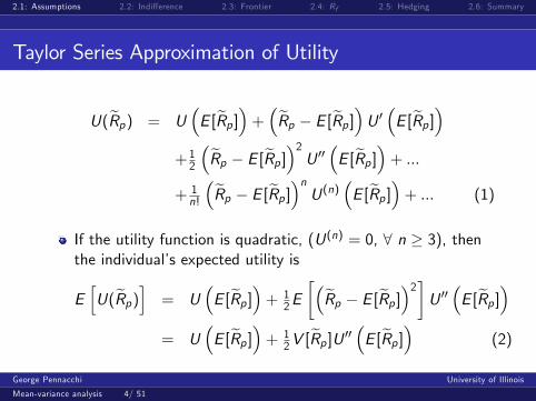
Taylor Series Approximation of Utility
U(eRp) = U�E [eRp ]�+ �eRp � E [eRp ]�U 0 �E [eRp ]�
+12
�eRp � E [eRp ]�2 U 00 �E [eRp ]�+ :::+ 1n!
�eRp � E [eRp ]�n U(n) �E [eRp ]�+ ::: (1)
If the utility function is quadratic, (U(n) = 0, 8 n � 3), thenthe individual�s expected utility is
EhU(eRp)i = U
�E [eRp ]�+ 1
2E��eRp � E [eRp ]�2�U 00 �E [eRp ]�
= U�E [eRp ]�+ 1
2V [eRp ]U 00 �E [eRp ]� (2)
George Pennacchi University of Illinois
Mean-variance analysis 4/ 51

2.1: Assumptions 2.2: Indi¤erence 2.3: Frontier 2.4: Rf 2.5: Hedging 2.6: Summary
Alternative Utilities
Quadratic utility is problematic: it has a �bliss point� afterwhich utility declines in wealth.
Suppose, instead, we assume general increasing, concaveutility but restrict the probability distribution of the riskyassets.
Claim: If individual assets have a multi-variate normaldistribution, utility of wealth depends only on portfolio meanand variance.
Why? First note that the return on a portfolio is a weightedaverage (sum) of the returns on the individual assets.
Because sums of normals are normal, if the joint distributionsof individual assets are multivariate normal, then the portfolioreturn is also normally distributed.
George Pennacchi University of Illinois
Mean-variance analysis 5/ 51
2.1: Assumptions 2.2: Indi¤erence 2.3: Frontier 2.4: Rf 2.5: Hedging 2.6: Summary
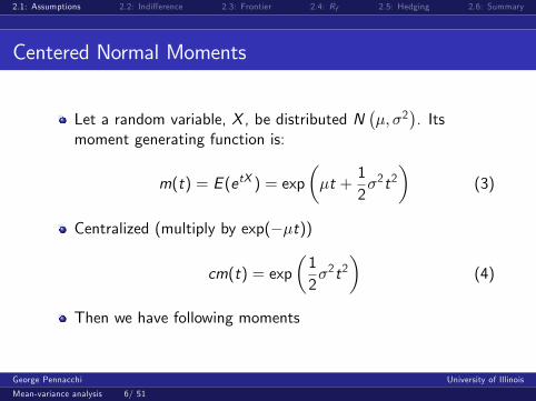
Centered Normal Moments
Let a random variable, X , be distributed N��; �2
�. Its
moment generating function is:
m(t) = E (etX ) = exp��t +
12�2t2
�(3)
Centralized (multiply by exp(��t))
cm(t) = exp�12�2t2
�(4)
Then we have following moments
George Pennacchi University of Illinois
Mean-variance analysis 6/ 51

2.1: Assumptions 2.2: Indi¤erence 2.3: Frontier 2.4: Rf 2.5: Hedging 2.6: Summary
Centered Normal Moments
E [eRp � �]1 =d exp
� 12�
2t2�
dt
�����t=0
= 0 (5)
E [eRp � �]2 =d2 exp
� 12�
2t2�
dt2
�����t=0
= �2
E [eRp � �]3 =d3 exp
� 12�
2t2�
dt3
�����t=0
= 0
E [eRp � �]4 =d4 exp
� 12�
2t2�
dt4
�����t=0
= 3�4
: : :
George Pennacchi University of Illinois
Mean-variance analysis 7/ 51
2.1: Assumptions 2.2: Indi¤erence 2.3: Frontier 2.4: Rf 2.5: Hedging 2.6: Summary
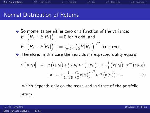
Normal Distribution of Returns
So moments are either zero or a function of the variance:Eh�eRp � E [eRp ]�ni = 0 for n odd, and
Eh�eRp � E [eRp ]�ni = n!
(n=2)!
�12V [
eRp ]�n=2 for n even.Therefore, in this case the individual�s expected utility equals
EhU(eRp)i = U
�E [eRp ]�+ 1
2V [eRp ]U 00 �E [eRp ]�+ 0 + 1
8
�V [eRp ]�2 U 0000 �E [eRp ]�
+0 + :::+1
(n=2)!
�1
2V [eRp ]�n=2 U (n) �E [eRp ]�+ ::: (6)
which depends only on the mean and variance of the portfolio
return.
George Pennacchi University of Illinois
Mean-variance analysis 8/ 51

2.1: Assumptions 2.2: Indi¤erence 2.3: Frontier 2.4: Rf 2.5: Hedging 2.6: Summary
Caveats
But is a multivariate normal distribution realistic for assetreturns?
If individual assets and eRp are normally distributed, the grossreturn will be negative with positive probility because thenormal distribution ranges over the entire real line.
This is a problem since most assets are limited liability, i.e.eRp � 0.Later, in a continuous-time context, we can assume assetreturns are instantaneously normal, which allows them to belog-normally distributed over �nite intervals.
George Pennacchi University of Illinois
Mean-variance analysis 9/ 51

2.1: Assumptions 2.2: Indi¤erence 2.3: Frontier 2.4: Rf 2.5: Hedging 2.6: Summary
Preference for Return Mean and Variance
Therefore, assume U is a general utility function and assetreturns are normally distributed. The portfolio return ~Rp hasnormal probability density function f (R; �Rp ; �2p), where wede�ne �Rp � E [~Rp ] and �2p � V [~Rp ].Expected utility can then be written as
EhU�eRp�i = Z 1
�1U(R)f (R; �Rp ; �2p)dR (7)
Consider an individual�s indi¤erence curves. De�ne ex� ~Rp��Rp
�p,
EhU�eRp�i = Z 1
�1U(�Rp + x�p)n(x)dx (8)
where n(x) � f (x ; 0; 1). (ex is a standardized normal)George Pennacchi University of Illinois
Mean-variance analysis 10/ 51

2.1: Assumptions 2.2: Indi¤erence 2.3: Frontier 2.4: Rf 2.5: Hedging 2.6: Summary
Mean vs Variance cont�d
Taking the partial derivative with respect to �Rp :
@EhU�eRp�i
@ �Rp=
Z 1
�1U 0n(x)dx > 0 (9)
since U 0 is always greater than zero.
Taking the partial derivative of equation (8) with respect to�2p and using the chain rule:
@EhU�eRp�i
@�2p=
12�p
@EhU�eRp�i
@�p=
12�p
Z 1
�1U 0xn(x)dx
(10)
George Pennacchi University of Illinois
Mean-variance analysis 11/ 51

2.1: Assumptions 2.2: Indi¤erence 2.3: Frontier 2.4: Rf 2.5: Hedging 2.6: Summary
Risk and Utility
While U 0 is always positive, x ranges between �1 and +1.Take the positive and negative pair +xi and �xi . Thenn(+xi ) = n(�xi ). Comparing the integrand of equation (10)for equal absolute realizations of x , we can show
U 0(�Rp + xi�p)xin(xi ) + U 0(�Rp � xi�p)(�xi )n(�xi )= U 0(�Rp + xi�p)xin(xi )� U 0(�Rp � xi�p)xin(xi )= xin(xi )
�U 0(�Rp + xi�p)� U 0(�Rp � xi�p)
�< 0 (11)
becauseU 0(�Rp + xi�p) < U 0(�Rp � xi�p) (12)
due to the assumed concavity of U.
George Pennacchi University of Illinois
Mean-variance analysis 12/ 51

2.1: Assumptions 2.2: Indi¤erence 2.3: Frontier 2.4: Rf 2.5: Hedging 2.6: Summary
Risk and Utility cont�d
Thus, comparing U 0xin(xi ) for each positive and negative pair,we conclude that
@EhU�eRp�i
@�2p=
12�p
Z 1
�1U 0xn(x)dx < 0 (13)
which is intuitive for risk-averse vN-M individuals.An indi¤erence curve is the combinations of
��Rp ; �2p
�that
satisfy the equation EhU�eRp�i = U , a constant. Higher U
denotes greater utility. Taking the derivative
dEhU�eRp�i = @E
hU�eRp�i
@�2pd�2p +
@EhU�eRp�i
@ �Rpd �Rp = 0
(14)
George Pennacchi University of Illinois
Mean-variance analysis 13/ 51

2.1: Assumptions 2.2: Indi¤erence 2.3: Frontier 2.4: Rf 2.5: Hedging 2.6: Summary
Mean and Variance Indi¤erence Curve
Rearranging the terms of dEhU�eRp�i = 0, we obtain:
d �Rpd�2p
= �@EhU�eRp�i
@�2p=@EhU�eRp�i
@ �Rp> 0 (15)
since we showed@E [U(eRp)]
@�2p< 0 and
@E [U(eRp)]@ �Rp
> 0.
Hence, each indi¤erence curve is positively sloped in��Rp ; �2p
�space. They cannot intersect because since we showed thatutility is increasing in expected portfolio return for a givenlevel of portfolio standard deviation.
George Pennacchi University of Illinois
Mean-variance analysis 14/ 51

2.1: Assumptions 2.2: Indi¤erence 2.3: Frontier 2.4: Rf 2.5: Hedging 2.6: Summary
Mean and Standard Deviation Indi¤erence Curve
As an exercise, show that the indi¤erence curve is upwardsloping and convex in
��Rp ; �p
�space:
George Pennacchi University of Illinois
Mean-variance analysis 15/ 51

2.1: Assumptions 2.2: Indi¤erence 2.3: Frontier 2.4: Rf 2.5: Hedging 2.6: Summary
Tangency Portfolios
The individual�s optimal choice of portfolio mean and varianceis determined by the point where one of these indi¤erencecurves is tangent to the set of means and standard deviationsfor all feasible portfolios, what we might describe as the �riskversus expected return investment opportunity set.�
This set represents all possible ways of combining variousindividual assets to generate alternative combinations ofportfolio mean and variance (or standard deviation).
The set includes ine¢ cient portfolios (those in the interior ofthe opportunity set) as well as e¢ cient portfolios (those onthe �frontier�of the set).
How can one determine e¢ cient portfolios?
George Pennacchi University of Illinois
Mean-variance analysis 16/ 51
2.1: Assumptions 2.2: Indi¤erence 2.3: Frontier 2.4: Rf 2.5: Hedging 2.6: Summary
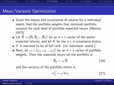
Mean/Variance Optimization
Given the means and covariances of returns for n individualassets, �nd the portfolio weights that minimize portfoliovariance for each level of portfolio expected return (Merton,1972).Let �R = (�R1 �R2 ::: �Rn)0 be an n � 1 vector of the assets�expected returns, and let V be the n � n covariance matrix.V is assumed to be of full rank. (no redundant assets.)Next, let ! = (!1 !2 ::: !n)0 be an n � 1 vector of portfolioweights. Then the expected return on the portfolio is
�Rp = !0 �R (16)
and the variance of the portfolio return is
�2p = !0V! (17)
George Pennacchi University of Illinois
Mean-variance analysis 17/ 51

2.1: Assumptions 2.2: Indi¤erence 2.3: Frontier 2.4: Rf 2.5: Hedging 2.6: Summary
Mean/Variance Optimization cont�d
The constraint on portfolio weights is !0e = 1 where e isde�ned as an n � 1 vector of ones.A frontier portfolio minimizes the portfolio�s variance subjectto the constraints that the portfolio�s expected return equalsRp and the portfolio�s weights sum to one:
min!
12!
0V! + ��Rp � !0 �R
�+ [1� !0e] (18)
The �rst-order conditions with respect to !, �, and , are
V! � ��R � e = 0 (19)
Rp � !0 �R = 0 (20)
1� !0e = 0 (21)
George Pennacchi University of Illinois
Mean-variance analysis 18/ 51

2.1: Assumptions 2.2: Indi¤erence 2.3: Frontier 2.4: Rf 2.5: Hedging 2.6: Summary
Mean/Variance Optimization cont�d
Solving (19) for !�, the portfolio weights are
!� = �V�1 �R + V�1e (22)
Pre-multiplying equation (22) by �R 0 and e 0 respectively:
Rp = �R 0!� = ��R 0V�1 �R + �R 0V�1e (23)
1 = e 0!� = �e 0V�1 �R + e 0V�1e (24)
Solving equations (23) and (24) for � and :
� =�Rp � �&� � �2 (25)
=& � �Rp&� � �2 (26)
George Pennacchi University of Illinois
Mean-variance analysis 19/ 51

2.1: Assumptions 2.2: Indi¤erence 2.3: Frontier 2.4: Rf 2.5: Hedging 2.6: Summary
Mean/Variance Optimization cont�d
Here � �= e 0V�1 �R, & � �R 0V�1 �R, and � � e 0V�1e arescalars.
The denominators &� � �2 are positive. Since V is positivede�nite, so is V�1. Therefore, the quadratic form��R � &e
�0V�1
��R � &e
�= �2& � 2�2& + &2� = &
�&� � �2
�is positive.
But since & � R 0V�1R is a positive quadratic form, then�&� � �2
�must also be positive.
Substituting for � and in equation (22), we have
!� =�Rp � �&� � �2 V
�1 �R +& � �Rp&� � �2 V
�1e (27)
George Pennacchi University of Illinois
Mean-variance analysis 20/ 51
2.1: Assumptions 2.2: Indi¤erence 2.3: Frontier 2.4: Rf 2.5: Hedging 2.6: Summary
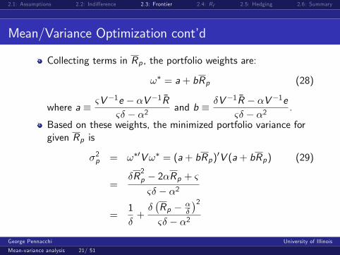
Mean/Variance Optimization cont�d
Collecting terms in Rp , the portfolio weights are:
!� = a+ bRp (28)
where a � &V�1e � �V�1 �R&� � �2 and b � �V�1 �R � �V�1e
&� � �2 .
Based on these weights, the minimized portfolio variance forgiven Rp is
�2p = !�0V!� = (a+ bRp)0V (a+ bRp) (29)
=�R
2p � 2�Rp + &&� � �2
=1�+��Rp � �
�
�2&� � �2
George Pennacchi University of Illinois
Mean-variance analysis 21/ 51
2.1: Assumptions 2.2: Indi¤erence 2.3: Frontier 2.4: Rf 2.5: Hedging 2.6: Summary
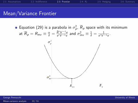
Mean/Variance Frontier
Equation (29) is a parabola in �2p , Rp space with its minimum
at Rp = Rmv � �� =
�R 0V�1ee 0V�1e and �
2mv � 1
� =1
e 0V�1e .
George Pennacchi University of Illinois
Mean-variance analysis 22/ 51

2.1: Assumptions 2.2: Indi¤erence 2.3: Frontier 2.4: Rf 2.5: Hedging 2.6: Summary
Mean/Variance Optimization cont�d
Substituting Rp = �� into equation (27) and multiplying by
��
shows that this minimum variance portfolio has weights!mv =
1�V
�1e = V�1e=�e 0V�1e
�.
An investor whose utility is increasing in expected portfolioreturn and is decreasing in portfolio variance would neverchoose a portfolio having Rp < Rmv .
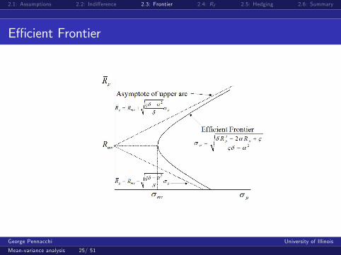
Hence, the e¢ cient portfolio frontier is represented only bythe region Rp � Rmv .Next, let us plot the frontier in �p , Rp space by taking thesquare root of both sides of equation (29):
George Pennacchi University of Illinois
Mean-variance analysis 23/ 51

2.1: Assumptions 2.2: Indi¤erence 2.3: Frontier 2.4: Rf 2.5: Hedging 2.6: Summary
Asymptotes
�p =
s1�+��Rp � �
�
�2&� � �2
which is a hyperbola in �p , Rp space. Di¤erentiating, thishyperbola�s slope can be written as
@Rp@�p
=&� � �2
��Rp � �
�
��p (30)
The hyperbola�s e¢ cient (ine¢ cient) upper (lower) arc
asymptotes to the straight line Rp = Rmv +q
&���2� �p
(Rp = Rmv �q
&���2� �p).
George Pennacchi University of Illinois
Mean-variance analysis 24/ 51
2.1: Assumptions 2.2: Indi¤erence 2.3: Frontier 2.4: Rf 2.5: Hedging 2.6: Summary
E¢ cient Frontier
George Pennacchi University of Illinois
Mean-variance analysis 25/ 51
2.1: Assumptions 2.2: Indi¤erence 2.3: Frontier 2.4: Rf 2.5: Hedging 2.6: Summary
Two Fund Separation
We now state and prove a fundamental result:
TheoremEvery portfolio on the mean-variance frontier can be replicated bya combination of any two frontier portfolios; and an individual willbe indi¤erent between choosing among the n �nancial assets, orchoosing a combination of just two frontier portfolios.
The implication is that if a security market o¤ered two mutualor �exchange-traded� funds, each invested in a di¤erentfrontier portfolio, any mean-variance investor could replicatehis optimal portfolio by appropriately dividing his wealthbetween only these two funds. (He may have to short one.)
George Pennacchi University of Illinois
Mean-variance analysis 26/ 51

2.1: Assumptions 2.2: Indi¤erence 2.3: Frontier 2.4: Rf 2.5: Hedging 2.6: Summary
Two Fund Separation: Proof
Proof: Let �R1p , �R2p and �R3p be the expected returns on threefrontier portfolios. Invest a proportion of wealth, x , inportfolio 1 and the remainder, (1� x), in portfolio 2 such that:
�R3p = x �R1p + (1� x)�R2p (31)
Recall that the weights of frontier portfolios 1 and 2 are!1 = a+ b�R1p and !2 = a+ b�R2p , respectively. Hence,Portfolio 3�s weights are
x!1 + (1� x)!2 = x(a+ b�R1p) + (1� x)(a+ b�R2p)(32)= a+ b(x �R1p + (1� x)�R2p)= a+ b�R3p = !3
which shows it is also a frontier portfolio.
George Pennacchi University of Illinois
Mean-variance analysis 27/ 51

2.1: Assumptions 2.2: Indi¤erence 2.3: Frontier 2.4: Rf 2.5: Hedging 2.6: Summary
Zero Covariance Portfolios
Frontier portfolios have another property. Except for theminimum variance portfolio, !mv , for each frontier portfoliothere is another frontier portfolio with which its returns havezero covariance:
!10V!2 = (a+ bR1p)0V (a+ bR2p) (33)
=1�+
�
&� � �2�R1p �
�
�
��R2p �
�
�
�Equating this to zero and solving for R2p in terms of Rmv � �
� ,
R2p =�
�� &� � �2
�2�R1p � �
�
� (34)
= Rmv �&� � �2
�2�R1p � Rmv
�George Pennacchi University of Illinois
Mean-variance analysis 28/ 51
2.1: Assumptions 2.2: Indi¤erence 2.3: Frontier 2.4: Rf 2.5: Hedging 2.6: Summary
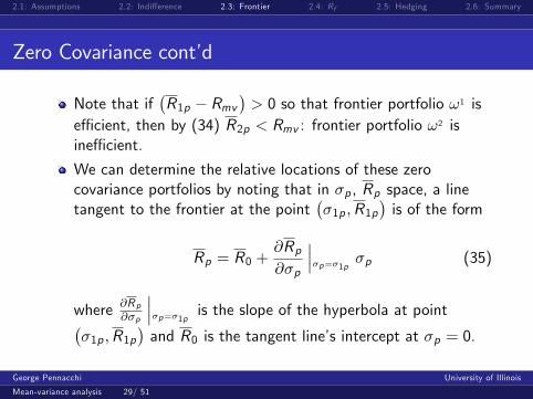
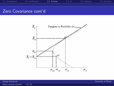
Zero Covariance cont�d
Note that if�R1p � Rmv
�> 0 so that frontier portfolio !1 is
e¢ cient, then by (34) R2p < Rmv : frontier portfolio !2 isine¢ cient.
We can determine the relative locations of these zerocovariance portfolios by noting that in �p , Rp space, a linetangent to the frontier at the point
��1p ;R1p
�is of the form
Rp = R0 +@Rp@�p
����p=�1p �p (35)
where @R p@�p
����p=�1p is the slope of the hyperbola at point��1p ;R1p
�and R0 is the tangent line�s intercept at �p = 0.
George Pennacchi University of Illinois
Mean-variance analysis 29/ 51

2.1: Assumptions 2.2: Indi¤erence 2.3: Frontier 2.4: Rf 2.5: Hedging 2.6: Summary
Zero Covariance cont�d
Using (30) and (29), we can solve for R0 by evaluating (35)at the point
��1p ;R1p
�:
R0 = R1p �@Rp@�p
����p=�1p �1p = R1p � &� � �2
��R1p � �
�
��1p�1p= R1p �
&� � �2
��R1p � �
�
� "1�+��R1p � �
�
�2&� � �2
#
=�
�� &� � �2
�2�R1p � �
�
� (36)
= R2p
The intercept of the line tangent to !1 is the expected returnof its zero-covariance counterpart, !2 .
George Pennacchi University of Illinois
Mean-variance analysis 30/ 51
2.1: Assumptions 2.2: Indi¤erence 2.3: Frontier 2.4: Rf 2.5: Hedging 2.6: Summary
Zero Covariance cont�d
George Pennacchi University of Illinois
Mean-variance analysis 31/ 51
2.1: Assumptions 2.2: Indi¤erence 2.3: Frontier 2.4: Rf 2.5: Hedging 2.6: Summary
E¢ cient Frontier with a Riskless Asset
Assume there is a riskless asset with return Rf (Tobin, 1958).Now, the constraint !0e = 1 does not apply because 1� !0eis the portfolio proportion invested in the riskless asset.However, we can now write expected return on the portfolio as
�Rp = Rf + !0(�R � Rf e) (37)
The variance of the return on the portfolio is still !0V!.Thus, the individual�s optimization problem is changed to:
min!
12!
0V! + ��Rp �
�Rf + !0(�R � Rf e)
�(38)
Similar to the previous derivation, the solution to the �rstorder conditions is
!� = �V�1(�R � Rf e) (39)
George Pennacchi University of Illinois
Mean-variance analysis 32/ 51

2.1: Assumptions 2.2: Indi¤erence 2.3: Frontier 2.4: Rf 2.5: Hedging 2.6: Summary
E¢ cient Frontier with a Riskless Asset
Here � � R p�Rf(�R�Rf e)
0V�1(�R�Rf e)
=R p�Rf
&�2�Rf+�R 2f,and the variance
of the frontier portfolio in terms of !� is
�2p = !�0V !� =R p � Rf�
�R � Rf e�0 V�1(�R � Rf e) (�R � Rf e)0V�1V �
R p � Rf��R � Rf e
�0 V�1(�R � Rf e)V�1(�R � Rf e)=
(R p � Rf )2��R � Rf e
�0 V�1(�R � Rf e) = (R p � Rf )2
& � 2�Rf + �R 2f(40)
Taking the square root of (40) and rearranging:
Rp = Rf ��& � 2�Rf + �R2f
� 12 �p (41)
which indicates that the frontier is now linear in �p , Rp space.
George Pennacchi University of Illinois
Mean-variance analysis 33/ 51

2.1: Assumptions 2.2: Indi¤erence 2.3: Frontier 2.4: Rf 2.5: Hedging 2.6: Summary
E¢ cient Frontier with a Riskless Asset
George Pennacchi University of Illinois
Mean-variance analysis 34/ 51

2.1: Assumptions 2.2: Indi¤erence 2.3: Frontier 2.4: Rf 2.5: Hedging 2.6: Summary
Two Fund Separation: Rf < Rmv
When Rf 6= Rmv � �� , an even stronger separation principle
obtains: any frontier portfolio can be replicated with oneportfolio that is located on the "risky asset only" frontier andanother portfolio that holds only the riskless asset.
Let us prove this result for the case Rf < Rmv . We assert that
the e¢ cient frontier line Rp = Rf +�& � 2�Rf + �R2f
� 12 �p
can be replicated by a portfolio consisting of only the risklessasset and a portfolio on the risky-asset-only frontier that isdetermined by a straight line tangent to this frontier whoseintercept is Rf .
If we show that the slope of this tangent is�& � 2�Rf + �R2f
� 12 , the assertion is proved.
George Pennacchi University of Illinois
Mean-variance analysis 35/ 51

2.1: Assumptions 2.2: Indi¤erence 2.3: Frontier 2.4: Rf 2.5: Hedging 2.6: Summary
Two Fund Separation: Rf < Rmv
Let RA and �A be the expected return and standard deviationof return, respectively, of this tangency portfolio. Then theresults of (34) and (35) allow us to write the tangent�s slopeas
Slope � RA � Rf�A
=
"�
�� &� � �2
�2�Rf � �
�
� � Rf#=�A
=
"2�Rf � & � �R2f��Rf � �
�
� #=�A (42)
Furthermore, we can use (29) and (34) to write
�2A =1�+��RA � �
�
�2&� � �2
George Pennacchi University of Illinois
Mean-variance analysis 36/ 51

2.1: Assumptions 2.2: Indi¤erence 2.3: Frontier 2.4: Rf 2.5: Hedging 2.6: Summary
Two Fund Separation: Rf < Rmv cont�d
We then substitute (34) where R1p = Rf for RA
�2A =1�+
&� � �2
�3�Rf � �
�
�2=
�R2f � 2�Rf + &�2�Rf � �
�
�2 (43)
Substituting the square root of (43) into (42):
RA � Rf�A
=
"2�Rf � & � �R2f��Rf � �
�
� #���Rf � �
�
���R2f � 2�Rf + &
� 12
(44)
=��R2f � 2�Rf + &
� 12
which is the desired result.George Pennacchi University of Illinois
Mean-variance analysis 37/ 51

2.1: Assumptions 2.2: Indi¤erence 2.3: Frontier 2.4: Rf 2.5: Hedging 2.6: Summary
An Important Separation Result
This result implies that all investors choose to hold riskyassets in the same relative proportions given by the tangencyportfolio !A. Investors di¤er only in the proportion of wealthallocated to this portfolio versus the risk-free asset.
George Pennacchi University of Illinois
Mean-variance analysis 38/ 51

2.1: Assumptions 2.2: Indi¤erence 2.3: Frontier 2.4: Rf 2.5: Hedging 2.6: Summary
Level of Risk-free Return
Rf < Rmv is required for asset market equilibrium. If
Rf > Rmv , the e¢ cient frontier
Rp = Rf +�& � 2�Rf + �R2f
� 12 �p is always above the
risky-asset-only frontier, implying the investor short-sells thetangency portfolio on the ine¢ cient risky asset frontier andinvests the proceeds in the risk-free asset.
George Pennacchi University of Illinois
Mean-variance analysis 39/ 51

2.1: Assumptions 2.2: Indi¤erence 2.3: Frontier 2.4: Rf 2.5: Hedging 2.6: Summary
Level of Risk-free Return
If Rf = Rmv the portfolio frontier is given by the asymptotesof the risky frontier. Setting Rf = Rmv in (39) andpremultiplying by e:
!� =Rp � Rf
& � 2�Rf + �R2fV�1(�R � Rf e) (45)
e 0!� = e 0V�1(�R � ��e)
Rp � Rf& � 2�Rf + �R2f
e 0!� = (�� ���)
Rp � Rf& � 2�Rf + �R2f
= 0
which shows that total wealth is invested in the risk-free asset.However, the investor also holds a risky, but zero net wealth,position in risky assets by short-selling particular risky assetsto �nance long positions in other risky assets.
George Pennacchi University of Illinois
Mean-variance analysis 40/ 51

2.1: Assumptions 2.2: Indi¤erence 2.3: Frontier 2.4: Rf 2.5: Hedging 2.6: Summary
Example with Negative Exponential Utility
Given a speci�c utility function and normally distributed assetreturns, optimal portfolio weights can be derived directly bymaximizing expected utility:
U( ~W ) = �e�b ~W (46)
where b is the individual�s coe¢ cient of absolute risk aversion.Now de�ne br � bW0, which is the individual�s coe¢ cient ofrelative risk aversion at initial wealth W0. Equation (46) canbe rewritten:
U( ~W ) = �e�br ~W =W0 = �e�br ~Rp (47)
where ~Rp is the total return (one plus the rate of return) onthe portfolio.
George Pennacchi University of Illinois
Mean-variance analysis 41/ 51

2.1: Assumptions 2.2: Indi¤erence 2.3: Frontier 2.4: Rf 2.5: Hedging 2.6: Summary
Example with Negative Exponential Utility cont�d
We still have n risky assets and Rf as before. Now recall theproperties of the lognormal distribution. If ~x is a normallydistributed random variable, for example, ~x � N(�; �2), then~z = eex is lognormally distributed. The expected value of ez is
E [~z ] = e�+12�
2(48)
From (47), we see that if ~Rp = Rf + !0(~R � Rf e) is normallydistributed, then U
�~W�is lognormally distributed. Using
equation (48), we have
EhU�fW�i = �e�br [Rf+!0(�R�Rf e)]+ 1
2 b2r !
0V ! (49)
The individual chooses portfolio weights to maximize expectedutility:
George Pennacchi University of Illinois
Mean-variance analysis 42/ 51
2.1: Assumptions 2.2: Indi¤erence 2.3: Frontier 2.4: Rf 2.5: Hedging 2.6: Summary
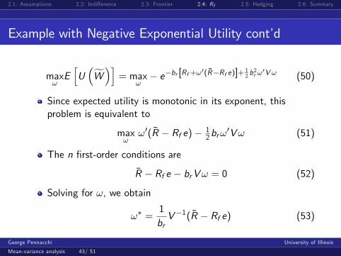
Example with Negative Exponential Utility cont�d
max!EhU�fW�i = max
!� e�br [Rf+!0(�R�Rf e)]+
12 b
2r !
0V ! (50)
Since expected utility is monotonic in its exponent, thisproblem is equivalent to
max!!0(�R � Rf e)� 1
2br!0V! (51)
The n �rst-order conditions are
�R � Rf e � brV! = 0 (52)
Solving for !, we obtain
!� =1brV�1(�R � Rf e) (53)
George Pennacchi University of Illinois
Mean-variance analysis 43/ 51
2.1: Assumptions 2.2: Indi¤erence 2.3: Frontier 2.4: Rf 2.5: Hedging 2.6: Summary
Example with Negative Exponential Utility cont�d
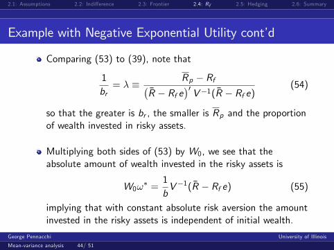
Comparing (53) to (39), note that
1br= � � Rp � Rf�
�R � Rf e�0 V�1(�R � Rf e) (54)
so that the greater is br , the smaller is Rp and the proportionof wealth invested in risky assets.
Multiplying both sides of (53) by W0, we see that theabsolute amount of wealth invested in the risky assets is
W0!� =
1bV�1(�R � Rf e) (55)
implying that with constant absolute risk aversion the amountinvested in the risky assets is independent of initial wealth.
George Pennacchi University of Illinois
Mean-variance analysis 44/ 51

2.1: Assumptions 2.2: Indi¤erence 2.3: Frontier 2.4: Rf 2.5: Hedging 2.6: Summary
Cross-hedging (Anderson & Danthine, 1981)
Consider a one-period model of an individual required to tradea commodity in the future and wants to hedge the risk usingfutures contracts.
Assume that at date 0 she is committed to buy (sell) y > 0(y < 0) units of a risky commodity at date 1 at the spot pricep1. As of date 0, y is deterministic, while p1 is stochastic.
There are n �nancial securities (futures contracts) where thedate 0 price of the i th �nancial security as psi0. Its risky date 1price is psi1.
Let si denote the amount of the i th security purchased at date0, where si < 0 indicates a short position.
George Pennacchi University of Illinois
Mean-variance analysis 45/ 51

2.1: Assumptions 2.2: Indi¤erence 2.3: Frontier 2.4: Rf 2.5: Hedging 2.6: Summary
Cross-hedging (Anderson & Danthine, 1981) cont�d
De�ne n � 1 quantity and price vectors s � [s1 ::: sn]0,ps0 � [ps10 ::: psn0]0, and ps1 � [ps11 ::: psn1]0. Also de�neps � ps1 � ps0 as the n � 1 vector of security price changes.Thus, the date 1 pro�t from securities trading is ps 0s
De�ne the moments E [p1] = �p1, Var [p1] = �00, E [ps1] = �ps1,
E [ps ] = �ps , Cov [psi1; psj1] = �ij , Cov [p1; p
si1] = �0i , and the
(n + 1)� (n + 1) covariance matrix of the spot commodityand �nancial securities is
� =
��00 �01�001 �11
�(56)
where �11 is an n � n matrix whose i ; j th element is �ij , and�01 is a 1� n vector whose i th element is �0i .
George Pennacchi University of Illinois
Mean-variance analysis 46/ 51
2.1: Assumptions 2.2: Indi¤erence 2.3: Frontier 2.4: Rf 2.5: Hedging 2.6: Summary
Cross-hedging (Anderson & Danthine, 1981) cont�d
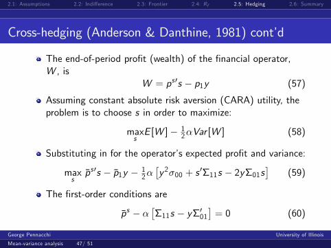
The end-of-period pro�t (wealth) of the �nancial operator,W , is
W = ps 0s � p1y (57)
Assuming constant absolute risk aversion (CARA) utility, theproblem is to choose s in order to maximize:
maxsE [W ]� 1
2�Var [W ] (58)
Substituting in for the operator�s expected pro�t and variance:
maxs�ps 0s � �p1y � 1
2��y2�00 + s 0�11s � 2y�01s
�(59)
The �rst-order conditions are
�ps � ���11s � y�001
�= 0 (60)
George Pennacchi University of Illinois
Mean-variance analysis 47/ 51
2.1: Assumptions 2.2: Indi¤erence 2.3: Frontier 2.4: Rf 2.5: Hedging 2.6: Summary
Cross-hedging (Anderson & Danthine, 1981) cont�d
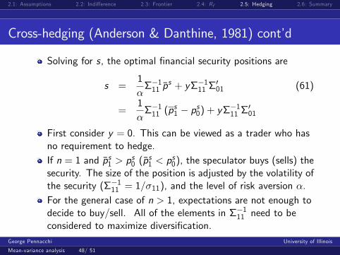
Solving for s, the optimal �nancial security positions are
s =1���111 �p
s + y��111 �001 (61)
=1���111 (p
s1 � ps0) + y��111 �
001
First consider y = 0. This can be viewed as a trader who hasno requirement to hedge.If n = 1 and �ps1 > p
s0 (�p
s1 < p
s0), the speculator buys (sells) the
security. The size of the position is adjusted by the volatility ofthe security (��111 = 1=�11), and the level of risk aversion �.For the general case of n > 1, expectations are not enough todecide to buy/sell. All of the elements in ��111 need to beconsidered to maximize diversi�cation.
George Pennacchi University of Illinois
Mean-variance analysis 48/ 51

2.1: Assumptions 2.2: Indi¤erence 2.3: Frontier 2.4: Rf 2.5: Hedging 2.6: Summary
Cross-hedging (Anderson & Danthine, 1981) cont�d
For the general case y 6= 0, the situation faced by a hedger,the demand for �nancial securities is similar to that of a purespeculator in that it also depends on price expectations.In addition, there are hedging demands, call them sh :
sh � y��111 �001 (62)
This is the solution to the variance-minimization problem, yetin general expected returns matter for hedgers.From (62), note that when n = 1 the pure hedging demandper unit of the commodity purchased, sh=y , is
sh
y=Cov(p1; ps1)Var(ps1)
(63)
George Pennacchi University of Illinois
Mean-variance analysis 49/ 51
2.1: Assumptions 2.2: Indi¤erence 2.3: Frontier 2.4: Rf 2.5: Hedging 2.6: Summary
Cross-hedging (Anderson & Danthine, 1981) cont�d
For the general case, n > 1, the elements of the vector��111 �
001 equal the coe¢ cients �1; :::; �n in the multiple
regression model:
�p1 = �0 + �1�ps1 + �2�p
s2 + :::+ �n�p
sn + " (64)
where �p1 � p1 � p0, �psi � ps1i � ps0i , and " is a mean-zeroerror term.
An implication of (64) is that an operator might estimate thehedge ratios, sh=y , by performing a statistical regression usinga historical time series of the n � 1 vector of security pricechanges. In fact, this is a standard way that practitionerscalculate hedge ratios.
George Pennacchi University of Illinois
Mean-variance analysis 50/ 51

2.1: Assumptions 2.2: Indi¤erence 2.3: Frontier 2.4: Rf 2.5: Hedging 2.6: Summary
Summary
Normal distribution of individual asset returns is su¢ cient formean-variance optimization to be valid.
Two e¢ cient portfolios are enough to span the entiremean-variance e¢ cient frontier.
When a riskless asset exists, only one e¢ cient portfolio(tangency portfolio) and the riskless asset is required to spanthe frontier.
Hedging can be expressed as an application of mean-varianceoptimization.
George Pennacchi University of Illinois
Mean-variance analysis 51/ 51


![Mean-Variance Portfolio Rebalancing with Transaction · PDF fileMean-Variance Portfolio Rebalancing with Transaction Costs ... (Leland [2000] or Donohue and Yip [2003]). ... mean-variance](https://static.fdocuments.in/doc/165x107/5aa9b2147f8b9a81188d1c27/mean-variance-portfolio-rebalancing-with-transaction-portfolio-rebalancing-with.jpg)