Mean Univariate- GARCH VaR portfolio optimization Actual ...
33
Mean univariate- GARCH VaR portfolio optimization: actual portfolio approach Article (Accepted Version) http://sro.sussex.ac.uk Rankovic, Vladimir, Drenovak, Mikica, Urosevic, Branko and Jelic, Ranko (2016) Mean univariate- GARCH VaR portfolio optimization: actual portfolio approach. Computers & Operations Research, 72. pp. 83-92. ISSN 0305-0548 This version is available from Sussex Research Online: http://sro.sussex.ac.uk/id/eprint/59655/ This document is made available in accordance with publisher policies and may differ from the published version or from the version of record. If you wish to cite this item you are advised to consult the publisher’s version. Please see the URL above for details on accessing the published version. Copyright and reuse: Sussex Research Online is a digital repository of the research output of the University. Copyright and all moral rights to the version of the paper presented here belong to the individual author(s) and/or other copyright owners. To the extent reasonable and practicable, the material made available in SRO has been checked for eligibility before being made available. Copies of full text items generally can be reproduced, displayed or performed and given to third parties in any format or medium for personal research or study, educational, or not-for-profit purposes without prior permission or charge, provided that the authors, title and full bibliographic details are credited, a hyperlink and/or URL is given for the original metadata page and the content is not changed in any way.
Transcript of Mean Univariate- GARCH VaR portfolio optimization Actual ...
Mean univariate GARCH VaR portfolio optimization: actual portfolio approach
Article (Accepted Version)
http://sro.sussex.ac.uk
Rankovic, Vladimir, Drenovak, Mikica, Urosevic, Branko and Jelic, Ranko (2016) Mean univariate- GARCH VaR portfolio optimization: actual portfolio approach. Computers & Operations Research, 72. pp. 83-92. ISSN 0305-0548
This version is available from Sussex Research Online: http://sro.sussex.ac.uk/id/eprint/59655/
This document is made available in accordance with publisher policies and may differ from the published version or from the version of record. If you wish to cite this item you are advised to consult the publisher’s version. Please see the URL above for details on accessing the published version.
Copyright and reuse: Sussex Research Online is a digital repository of the research output of the University.
Copyright and all moral rights to the version of the paper presented here belong to the individual author(s) and/or other copyright owners. To the extent reasonable and practicable, the material made available in SRO has been checked for eligibility before being made available.
Copies of full text items generally can be reproduced, displayed or performed and given to third parties in any format or medium for personal research or study, educational, or not-for-profit purposes without prior permission or charge, provided that the authors, title and full bibliographic details are credited, a hyperlink and/or URL is given for the original metadata page and the content is not changed in any way.

Author’s Accepted Manuscript
Mean Univariate- GARCH VaR portfoliooptimization: Actual portfolio approach
Vladimir Ranković, Mikica Drenovak, BrankoUrosevic, Ranko Jelic
PII: S0305-0548(16)30004-1DOI: http://dx.doi.org/10.1016/j.cor.2016.01.014Reference: CAOR3923
To appear in: Computers and Operation Research
Received date: 10 July 2015Revised date: 3 December 2015Accepted date: 24 January 2016
Cite this article as: Vladimir Ranković, Mikica Drenovak, Branko Urosevic andRanko Jelic, Mean Univariate- GARCH VaR portfolio optimization: Actualportfolio approach, Computers and Operation Research,http://dx.doi.org/10.1016/j.cor.2016.01.014
This is a PDF file of an unedited manuscript that has been accepted forpublication. As a service to our customers we are providing this early version ofthe manuscript. The manuscript will undergo copyediting, typesetting, andreview of the resulting galley proof before it is published in its final citable form.Please note that during the production process errors may be discovered whichcould affect the content, and all legal disclaimers that apply to the journal pertain.
www.elsevier.com/locate/caor

1
Mean-Univariate GARCH VaR portfolio optimization: Actual
portfolio approach
Vladimir Rankovića)
, Mikica Drenovakb)
, Branko Urosevicc)
, and Ranko Jelicd) *
a) Faculty of Economics, University of Kragujevac, Djure Pucara 3, 34000 Kragujevac, Serbia;
E-mail: [email protected]. b) Faculty of Economics, University of Kragujevac, Djure Pucara 3, 34000 Kragujevac, Serbia;
E-mail: [email protected]. c) Faculty of Economics, University of Belgrade, Kamenicka 6, 11000 Beograd, Serbia; National Bank of Serbia, Kralja Petra
12, 11000 Beograd, Serbia; CESIfo Network, Poschinger Str. 5, 81679, Munich, Germany;
E-mail: [email protected].
*Corresponding author: d) School of Business, Management and Economics, University of Sussex, Sussex House, Falmer, Brighton, BN1 9RH UK;
E-mail: [email protected], Phone: +44 (0)121 4145990
Abstract
In accordance with Basel Capital Accords, the Capital Requirements (CR) for market risk
exposure of banks is a nonlinear function of Value-at-Risk (VaR). Importantly, the CR is
calculated based on a bank’s actual portfolio, i.e. the portfolio represented by its current
holdings. To tackle mean-VaR portfolio optimization within the actual portfolio framework
(APF), we propose a novel mean-VaR optimization method where VaR is estimated using a
univariate Generalized AutoRegressive Conditional Heteroscedasticity (GARCH) volatility
model. The optimization was performed by employing a Nondominated Sorting Genetic
Algorithm (NSGA-II). On a sample of 40 large US stocks, our procedure provided superior
mean-VaR trade-offs compared to those obtained from applying more customary mean-
multivariate GARCH and historical VaR models. The results hold true in both low and high
volatility samples.
KEY WORDS: Portfolio optimization, Actual portfolios, Value at Risk, GARCH, NSGA-II

2
1. Introduction
Value-at-Risk (VaR) is defined as the loss associated with the low (typically first or fifth)
percentile of the return distribution.1 The Basel II Capital Accord codifies VaR as the de-facto
industry standard for the banking and insurance industries alike (see, BIS [3, 4, 5]. In
particular, for the market risk exposure of banks, a bank’s internal VaR estimates
corresponding to the actual portfolio, i.e. the portfolio represented by its current holdings,
translate directly into the regulatory capital charge (see Hendricks and Hirtle [6]). Motivated
by this regulatory feature, we utilized the actual portfolio framework (APF) to determine a set
of portfolios characterized by the optimal trade-off between the expected return and VaR (i.e.
Pareto-optimal frontier). We further proposed a mean-univariate Generalized AutoRegressive
Conditional Heteroscedasticity (GARCH) VaR portfolio optimization model. We assumed that
portfolio returns, standardized by time varying volatility, have a conditional Student’s t
distribution, while conditional variance follows а GARCH (1, 1) process.2 The Student’s t
distribution efficiently captures the fat tails of standardized asset returns (see Christoffersen
[9], Huisman et al. [10]) whilst the GARCH model addresses issues related to volatility
clustering observed in the data.3 To the best of our knowledge, this is the first paper that
studies mean-VaR portfolio optimization using the actual portfolio approach and also the first
paper that uses the univariate GARCH VaR model in this context.
Previous studies on mean-VaR optimization implicitly assumed fixed weights (i.e. fractions of
assets) over the observed time period.4 Since prices change over time, maintaining the fixed
portfolio weights (FWA) requires frequent trading and leads to changes in the number of
shares of each asset in a portfolio. Regulatory capital charges, however, are determined by the
VaR of an actual portfolio where the number of shares of an asset (rather than its weighting) is
fixed over the observed period. It is, therefore, APF, rather than FWA, that is more relevant
for asset managers facing regulatory VaR limits. To illustrate the effectiveness of our APF
approach and univariate GARCH model, we compared our results with two benchmarks. Our
first benchmark is the mean-historical VaR approach developed in Rockafellar and Uryasev
[20, 21] and Krokhmal et al. [22]. These authors mapped conditional VaR (CVaR)
optimization into a linear programming problem and argued that the mean-CVaR efficient
1 For classification and comparison of risk measures see [1] and [2], among others.
2 GARCH was introduced in Engle [7] and GARCH (1, 1) in Bollerslev [8].
3 For more on superiority of GARCH VaR compared to historical VaR see [11], [12], [13], [14], [15], among
others. 4 For example, [16], [17], [18], [19], [20], [21].

3
frontier provided near-optimal solutions in the context of the mean-historical VaR trade-off.5
We referred to this benchmark as the Linear Programming (LP) model. The second point of
comparison for our approach is the mean-multivariate GARCH VaR optimization that can be
mapped into the Quadratic Programming (QP) problem (see Santos et al. [26]).
Use of the univariate GARCH approach for VaR modeling, however, makes the mean-VaR
optimization problem rather complex. Previous literature documented that Multi-Objective
Evolutionary Algorithms (MOEA) could reliably and efficiently be applied in complex
portfolio optimization problems.6
For example, Anagnostopoulos and Mamanis [31] studied
the effectiveness of different MOEA (e.g. Nondominated Sorting Genetic Algorithm (NSGA-
II), Strength Pareto Evolutionary Algorithm (SPEA2), Pareto Envelope-based Selection
Algorithm (PESA), etc.) in solving various complex mean-variance optimization problems.
They reported the best NSGA-II and SPEA2 average performance in terms of hypervolume
indicators, while PESA performed best in terms of the proximity to the Pareto-optimal
frontier. The same authors (see [32]) also examined the mean-variance, mean-ES, and mean-
VaR optimization problem with quantity, cardinality and class constraints. They showed that
NSGA-II, SPEA2 and PESA performed efficiently and their performance was independent of
the risk measure used.7 Deb et al. [34] reported NSGA-II’s advantages over the Pareto
Archived Evolutionary Strategy (PAES) and SPEA. Deb et al. [35] developed a hybrid NSGA-
II procedure for handling a mean-variance portfolio optimization problem with the cardinality
constraint and lower and upper bounds as investment criteria. The authors provided evidence
of NSGA-II’s superiority over classical quadratic programming approaches. Branke et al. [36]
considered the mean-variance problem with the maximum exposure constraint. The authors
generated mean-variance Pareto-optimal frontiers by using a hybrid algorithm that combined
NSGA-II with the critical line algorithm.
In this study we used the NSGA-II algorithm. Our choice was motivated by the above studies,
whose results highlighted the advantages of NSGA-II in tackling complex portfolio
5 CVaR (or Expected Shortfall, ES) is the expected loss, conditional that loss is higher than VaR. Thus, CVaR and
VaR are closely related risk measures. The LP model is widely used in CVaR and VaR optimization literature
(see [23], [24], [25], among others). 6 For comprehensive surveys of MOEA applications in portfolio optimization, see [27], [28], [29], [30].
7 Anagnostopoulos and Mamanis also showed that NSGA-II, SPEA2, and PESA provide a good approximation of
risk-return trade-offs in a 3 objectives optimization problem (see [33]).

4
optimization problems.8 NSGA-II was first introduced by Deb et al. [34] and subsequently
developed in Deb et al. [37]. Recently, a new version of NSGA (NSGA-III) was developed by
Deb and Jain [38] and also Jain and Deb [39]. NSGA-III is better suited to many-objective
optimization problems (three and more objectives) and offers the ability to define the desired
part of a solution space defined by reference points.9 Here, we prefer NSGA-II to NSGA-III,
since we consider only two objectives and are interested in the entire Pareto-optimal frontier.
Knowledge of the entire frontier of the risk-return trade-offs is particularly useful for asset
managers in banks and other financial institutions in order to comply with different in-house
and regulatory requirements.
For our numerical tests we selected 40 of the largest US stocks in the Standard and Poor’s
stock market index (S&P 100) for which sufficient data was available. First, we determined
the mean-historical VaR Pareto-optimal frontier, in the APF framework, using the NSGA-II
algorithm and compared it to the LP Pareto optimal frontier. The comparison showed that
NSGA-II produced better mean-historical VaR trade-offs compared to the LP optimization
approach, in both Low and High volatility samples. Second, we compared our mean-
univariate GARCH VaR Pareto-optimal frontier with the frontiers obtained by the two
benchmarks (mean-historical VaR and mean-multivariate GARCH VaR). In comparison with
the two benchmarks, the proposed univariate GARCH VaR procedure provided actual
portfolios with better mean-univariate GARCH VaR trade-offs, in both Low and High
volatility samples.
Previous portfolio optimization studies typically neglect the differences between using
portfolios with fixed weights and portfolios with fixed holdings of assets. We contribute to
portfolio optimization literature by addressing recent real world regulatory changes which
impose VaR based on actual portfolio holdings. The rare MOEA portfolio optimization studies
that measured risk by using VaR tend to use historical rather than analytical VaR (see
Anagnostopoulos and Mamanis [33], Hochreiter et al. [41], Soler et al. [42], Rankovic et al.
8 NSGA-II algorithm is also the most widely used MOEA in portfolio optimization literature. According to the
number of studies reviewed in [30], NSGA-II was used in twice as many studies compared to second most
popular method (SPEA2). 9 The number of the Pareto optimal solutions could also be reduced by combination of NSGA-II with Data
Envelopment Analysis (see [40]).

5
[43]).10
We therefore also contribute to MOEA literature by examining the mean-VaR
optimization problem with analytical univariate GARCH VaR instead of historical VAR.
The remainder of this paper is organized as follows. In Section 2 we introduce historical and
GARCH VaR models. The optimization problem is introduced in Section 3. MOAE and
implementation details are discussed in Section 4. Section 5 contains sample descriptive
statistics. Results of mean-historical VaR optimization are presented in Section 6. Results of
our univariate and multivariate mean-GARCH VaR optimization are presented and discussed
in Section 7. We conclude in Section 8. All acronyms and notations are listed in Appendix.
2. VaR Models
2.1. Traditional (historical) VaR
For a given portfolio, significance level α and time horizon h, portfolio VaR is a loss that will
be exceeded, on average, only α100 percent of the time. If expressed in terms of portfolio
value, VaR is the α-quantile of profit and loss distribution (cash VaR), while if expressed in
terms of portfolio return r, it is the α-quantile of the return distribution (relative VaR or,
simply, VaR). We focused on the α-quantile of the return distribution. Consider time horizon
of h=1 day and return rα such that probability ρ(r<rα) =α. In that case, 1-day VaR with
significance level α is:
VaR r
(1)
The minus sign is needed since VaR is defined as a loss. Given the cumulative distribution
function of returns F(α), the α-quantile is calculated as rα=F-1
(α). The main reason for the
popularity of this method is ease of its implementation and the fact that it makes no
assumptions about the parametric form of return distributions. On the other hand, the
historical VaR often slowly reacts to abrupt changes in market conditions (see Alexander
[11]).
10
Only 4.27% of MOEA studies use VaR as one of the objectives in the portfolio optimization problem (see
[27]).
6
2.2. Analytical VaR
A popular alternative to historical simulation is provided by analytical (or parametric) VaR
models. These models take a stand on the shape of the return distribution and capture the
following stylized facts about asset returns (see Christoffersen [9]). First, asset returns are
difficult to predict based on their past realizations. Second, volatility of daily returns
dominates their mean. Third, unlike returns, the variance of daily returns tends to exhibit
clustering over time. Namely, days with highly volatile returns are likely followed by days
with highly volatile returns and vice versa. Fourth, after periods of high or low asset volatility,
volatility tends to return toward a stable long run level. Fifth, even though asset returns are
often modeled using a normal distribution, an unconditional return distribution usually has
much heavier tails than predicted by a normal distribution.11
Using the first two conditional
moments of distribution, the return can be presented in the form:
t t t tr z (2)
where rt is the return at time t, μt is the conditional mean, σt is conditional volatility of the
return, and zt is the residual (innovation term) of the process. It is assumed that zt are
independently and identically distributed and follow a known theoretical distribution D with
zero mean and unit variance D (0, 1).
To specify the analytical VaR model we specified the volatility updating model, as well as the
shape of the conditional return distribution D (0, 1). A commonly applied class of conditional
volatility models that captures all of the above stylized facts of returns is the GARCH model.12
In estimating GARCH parameters on daily data, we have taken into account that the
conditional mean is dominated by the standard deviation of returns (see Christofferson [9],
Pritsker [15], Alexander [44]).13
This implies:
t t tr z (3)
We took into account non-normality of standardized returns by assuming they follow a
standardized Student’s t distribution (with zero mean and unit variance) with d degrees of
11
Although this is partially rectified when returns are standardized by time-varying volatility, some residual non-
normality still remains. 12
GARCH process was first applied to VaR modeling in [14]. 13
Alternatively, one can apply the same model to mean-adjusted returns.

7
freedom t (d). The degree of freedom parameter is an additional parameter estimated jointly
with the other model parameters using Maximum Likelihood Estimation (MLE) method. The
1-day ahead analytical VaR estimate with significance level α, calculated at time t, is obtained
as follows:
1
1 1 ( )t tVaR t d
(4)
where σt+1 is the 1-day ahead conditional volatility estimate at time t obtained by applying the
proposed model, d are degrees of freedom of the estimated Student’s t distribution of
standardized portfolio returns, and tα-1
(d) is α-quantile of the standardized Student’s t
distribution with d degrees of freedom.
Conditional portfolio volatility can be modeled directly using the time series of portfolio
returns (we referred to this method as the Univariate GARCH approach). Alternatively, one
can estimate conditional portfolio volatility using the conditional variance-covariance matrix
estimated via the multivariate GARCH model. We referred to this method as the multivariate
GARCH approach.
2.2.1. Univariate GARCH VaR
Consider the (univariate) time series of portfolio returns and denote by tr the portfolio return
at time t. The simplest and by far the most popular GARCH model of conditional volatility,
commonly referred to as GARCH (1, 1), has the following form (see Bollerslev [8]):
1
2 2 2
t ttr (5)
Here, θ, β >0 and θ+β<1.14
Thus, the univariate GARCH VaR is:
1/2
2 2 1
1 tt tVaR r t d
(6)
14
The second condition assures stationarity of the conditional volatility process.

8
2.2.2. Multivariate GARCH VaR
In a multivariate GARCH modeling framework, the 1-day ahead portfolio conditional
volatility can be estimated as a function of the returns on individual assets (from the
opportunity set) as follows:15
2
1 1t t t t w H w (7)
where Ht+1 is N×N conditional variance-covariance matrix of returns of individual assets, and
wt is the vector of portfolio weights at time t.16
Importantly, the multivariate GARCH
implicitly assumes a fixed portfolio weights approach (FWA). 17
The portfolio weights are
thus fixed at , ,i t i Tw w for all, , where T denotes optimization date. Thus, the
multivariate GARCH VaR is:
1/2 1
1 1 ( )t tVaR t d
w H w (8)
3. Optimization problem
3.1. Mean-univariate GARCH VaR optimization (APF approach)
The problem we are trying to solve has the following general form:
1/2
2 2 1
1min T T TVaR r t d
w
(9)
max E rw
(10)
1
subject to 1N
i
i
w
(11)
0 1, 1,...,iw i N (12)
Here, w denotes the vector of portfolio weights at optimization date t=T, its components are
wi, r is the return on the portfolio, denotes the portfolio risk measure that we try to
15
See, for example, [26] and [45]. 16
Boldface denotes matrices and vectors. Matrices are in upper case, whereas vectors are in lower case. 17
As discussed in [46], the fixed weights assumption further implies continuous portfolio rebalancing.

9
minimize, and E(r) is the expected return on the portfolio. tα-1
(d) here refers to a quantile of a
univariate Student’s t distribution with d degrees of freedom. Equation (11) describes the
standard budget constraint which requires that weights sum up to 1. Equation (12) states that
no short sales are allowed.18
To calculate actual portfolio VaR and the corresponding expected return, a time series of
portfolio returns with fixed asset holdings is needed. We determined asset holdings at the
optimization date by adopting an arbitrary dollar portfolio value (set, without loss of
generality, to 1). Thus, we assumed that, at optimization date t=Т, dollar portfolio value
Vp,t=T=1. Portfolio holdings ni at time T were determined based on weights at t=T:
,
, ,
i p t T ii
i t T i t T
wV wn
P P
(13)
Here Pi,t denotes the price of shares in company i at time t. In the actual portfolio approach,
holdings are held fixed over time. The actual portfolio return at time is, therefore,
determined as follows:
,
, 1
, 1, 1
1
1 1
N
i i tp t i
t N
p ti i t
i
n PV
rV
n P
(14)
Vp,t denotes the dollar portfolio value at time t. The actual portfolio mean-VaR optimization
problem simply means that we used equation (14) when determining input returns for the
above optimization problem.
In the actual portfolio approach, portfolio weights at time , are given by the expression:
,
,
,
1
i i t
i t N
i i t
i
n Pw
n P
(15)
Equations (14) and (15) imply that:
18
Short sale prohibition is a common constraint imposed on large institutional investors such as mutual or
pension funds.
10
, 1 ,
1
N
t i t i t
i
r w r
(16)
where ri,t is simple return on asset i at time t.
3.2. Mean - multivariate GARCH VaR optimization (FWA approach)
The portfolio optimization problem (Eq. (9) – (12)) can be specified as follows:
1/2 1
1 1min ( )T TVaR t d
ww H w (17)
subject to r w μ (18)
1
subject to 1N
i
i
w
(19)
0 1, 1,...,iw i N (20)
where HT+1 denotes the conditional variance-covariance matrix of individual returns estimated
at the time of optimization t=Т, μ denotes vector of expected returns of individual assets, and
r denotes the expected portfolio return as a weighted average of constituents’ expected
returns.
A portfolio return for an arbitrary, , is given by the expression:
, ,
1
N
t i T i t
i
r w r
(21)
Quantile tα-1
(d) refers to a quantile of a multivariate Student’s t distribution with d degrees of
freedom. Here, d does not depend on a portfolio composition. Namely, d and, thus, quantile tα-
1(d) depend solely on the choice of constituent return series and not on the way in which they
are combined into a particular portfolio. HT+1 and d are obtained using the Dynamic
Conditional Correlation (DCC) model of Engle [47].19
DCC decomposes conditional variance-covariance matrix Ht+1 into conditional standard
deviations and correlations, that is:
19
We used ‘rmgarch’ package [48] within software R [49]. For fitting GARCH model we used ‘dccfit’ method.
For the 1-day ahead estimation of conditional covariance matrix we used ‘dccforecast’ method.

11
1 1 1 1t t t t H D R D (22)
where Dt+1=diag( ,..., ). Here diag (*) is the operator transforming a N×1 vector
into a N×N diagonal matrix. We assume that conditional variances σ2
i,t+1, i = 1,..., N, follow a
standard univariate GARCH (1,1) model.
Matrix Rt+1 is a symmetric positive definite conditional correlation matrix defined as:
1/2 1/2
1 1 1 1t t t tdiag diag
R Q Q Q (23)
where Qt+1 is a proxy process which is assumed to follow GARCH-type dynamics:
1 1 T
t t t t Q Q z z Q (24)
Vector zt=(z1,t,...,zN,t)T has elements zi,t=ri,t/σi,t (standardized unexpected returns or
innovations), ̅ is the N×N covariance matrix of zt and θ and β are non-negative scalar
parameters satisfying θ+β<1.
Since tα-1
(d) is constant, the optimization problem (Eq. 17) is equivalent to a problem
represented by quadratic programming formulation (referred to as QP model):20
1min T
ww H w (25)
It should be emphasized that quantile tα-1
(d) in this approach is constant and therefore not
portfolio specific. Thus, the multivariate GARCH approach is more restrictive compared to
the univariate GARCH approach where the degrees of freedom of the estimated standardized
Student’s t distribution (and therefore quantile tα-1
(d)) were portfolio specific.
3.3. Summary of assumptions
3.3.1. General
i) Short sales are not allowed (Eqs. (12) and (21));
ii) The standard budget constraint which requires that weights must sum up to 1 (Eqs. (11)
and (20)).
20
This problem is of the standard Markowitz type (see [50]) with added short sales constraints.

12
3.3.2. Mean-univariate GARCH VaR optimization
i) Portfolio returns, standardized by time varying volatility, follow a conditional standardized
Student’s t distribution (with zero mean and unit variance);
ii) Conditional variance follows GARCH (1, 1) process, 1
2 2 2
t ttr , (Eq. 5);
iii) In estimating GARCH parameters on daily data, the mean value of daily returns is
dominated by the standard deviation of returns and that rt ≈ σt zt, (Eq. 3);
iv) At optimization date t=Т, without loss of generality, dollar portfolio value Vp,t=T =1.
3.3.3. Mean-multivariate GARCH VaR optimization
i) Portfolio weights are fixed over the observed period;
ii) Returns of assets from the opportunity set jointly follow a multivariate Student’s t
distribution;
iii) Qt+1 (Eq. 23) follows GARCH-type dynamics: 1 1 T
t t t t Q Q z z Q
iv) In matrix Dt+1 conditional variance σ2
i,t+1 follows a univariate GARCH (1, 1) process
4. Portfolio optimization methodology
4.1. Evolutionary algorithms (EA)
EA are efficient stochastic search techniques for solving complex optimization and search
problems (e.g., optimization problems with non-differentiable objective functions, large and
non-convex solution spaces, complex constraints etc.) through an emulation of natural
selection i.e. survival of the fittest (see Sastry et al. [51]). EA begin with a set of randomly
generated candidate solutions, referred to as a population. In each of the iterations (i.e.
generations) the following processes are performed: i) Good solutions from the current
population are selected and transferred into a set of potential parents (mating pool); ii)
Randomly selected parent solutions are combined (crossover) producing new solutions
(offspring solutions); iii) Some randomly selected offspring solutions are slightly modified
(mutation); iv) Generated offspring solutions constitute the population of the next generation.
By performing these processes in each generation (until the termination condition is satisfied)
the solutions ”evolve” and become even better in fulfilling the stated objectives.

13
Over the past two decades, significant advances have been made on EA methods to solve
multi-objective optimization problems.21
This has led to the creation of multi-objective
evolutionary algorithms (MOEA). In general, MOEA address two important issues: i) How to
generate a Pareto-optimal frontier; and ii) How to provide diversity in alternative solutions
(i.e. how to avoid convergence to a single point on the Pareto-optimal frontier). To achieve
the first goal, most MOEA implementations use ranking based on the concept of dominance,
while different diversity-preserving techniques are employed to achieve the second goal.
4.2. MOEA implementation
We directly borrowed the NSGA-II algorithm from Deb et al. [37].22
Implementation of
NSGA-II involves adopting settings for the solution representation, the population size, the
crossover and mutation probabilities and the termination condition. Solution representation
depends upon the specific optimization problem. For the model at hand, the solution was
defined as a non-negative real-valued vector of portfolio weights at time t=T, that is, the
vector of fractions of the total budget invested in individual securities (see Section 4).
Population size (the number of candidate portfolios in each generation), was set to 100. The
Pareto-optimal frontier was, therefore, approximated with 100 points. The step by step flow
chart which presents a schematic view of the proposed portfolio optimization method is
shown in Figure 1.
In the preparatory phase our software generated and printed a data file (data.csv) with a time
series of occurrences of assets under consideration. Next, it generated and printed an R script
file (Script.R) with commands for estimation of the univariate GARCH VaR. It then executed
the NSGA-II algorithm in the execution phase.23
21
For a detailed introduction to MOEA, see [52]. 22
The algorithm was coded in C# and run on a personal computer with Intel i5 processor and 4GB of RAM. 23
For more details on the algorithm steps, see [37].

14
Figure 1. Flow chart of the optimization algorithm
For the breeding of an offspring population we used the uniform crossover operator. Two
solutions (portfolios) from the current population were randomly selected and were
recombined with a predefined crossover probability. If the two solutions undergo
recombination, every allele(individual asset weight) is exchanged between the pair of
randomly selected solutions with a certain probability, known as the swapping probability,
otherwise, the two offspring are simply copies of their parents (see Sastry et al. [51]). 24
In
accordance with previous literature, we set the swapping probability to be 0.5.25
We applied a uniform mutation operator (uniform replacement). When applying uniform
mutation, each allele is selected with a predefined mutation probability and replaced with a
realization of a random variable, uniformly distributed in the range defined by the lower and
upper domain bounds. The selected crossover and mutation operator ensured that the
constraint defined by Eq. (12) was satisfied for each offspring. However, these operators did
not ensure satisfaction of the budget constraint (Eq.(11)). Hence, we had to normalize each of
the offspring solutions.26
In order to find the appropriate parameter values for the crossover and mutation probabilities,
we performed a series of experiments. The performance was assessed using the ε –indicator,
24
Candidate solutions are also referred to as chromosomes, decision variables are referred to as genes and the
values of decision variables are called alleles. 25
See [31], [32], [33], [51]. 26
We have done this by dividing each weight by sum of all weights.
15
and the hypervolume metric (see Zitzler et al. [53]). The ε -indicator is a binary performance
metric which is used to measure how close the approximation set is to the reference set. As a
reference set, the true or the best known Pareto-optimal frontier was used. The ε -indicator
determines a minimum value the reference set must be multiplied by in order for every
solution in the reference set to become weakly dominated by at least one solution in the
approximation set. If the approximation set matches the reference set exactly then the ε-
indicator takes the value of one. For this metric, values close to one indicate that the
approximation set very closely matches the reference set. The hypervolume indicator was
used to measure the diversity of the approximation set. The hypervolume measure quantifies
the volume of the objective space dominated by an approximation set. For optimization
problems with two objectives, it quantifies the area of the objective space dominated by the
approximation set, bounded by a predefined reference point. Thus, for this metric higher
values are preferable.
To determine the best performing mutation and crossover probability sets, we tested four
crossover probabilities (0.7, 0.8, 0.9, 1.0) and five uniform mutation probabilities (0.001,
0.005, 0.01, 0.05, 0.1). The above tests resulted in 20 different configurations for each set of
objectives (mean-historical VaR, mean-GARCH VaR) and for each data sample that we used.
For each configuration, the algorithm was left to run until 100,000 solutions were generated.
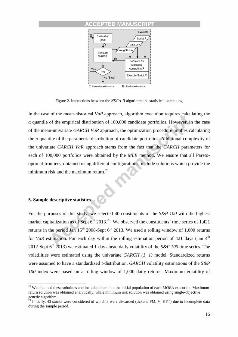
The interactions between the NSGA-II algorithm and our statistical analysis were highlighted
in Figure 2. For the evaluation of each individual solution portfolio, our software performed
the following steps: i) It generated and printed a file with portfolio weights (weights.csv); ii)
It called software R and executed the R script file (Script.R) created in the preparatory phase.
During the execution of the script file, software R used the data file (data.csv) and the solution
portfolio weights file (weights.csv) and generated a time series of actual portfolio returns
(applying Eq. (13) –(14)). Then VaR was estimated using the univariate GARCH model (Eq.
(4) and (5)). 27
27
We used ‘rugarch’ package [54] within software R [49]. For fitting GARCH model we used ‘ugarchfit’
method; For the 1-day ahead estimation of conditional volatility we used ‘ugarchforecast’ method.
16
Figure 2. Interactions between the NSGA-II algorithm and statistical computing
In the case of the mean-historical VaR approach, algorithm execution requires calculating the
α quantile of the empirical distribution of 100,000 candidate portfolios. However, in the case
of the mean-univariate GARCH VaR approach, the optimization procedure implies calculating
the α quantile of the parametric distribution of candidate portfolios. Additional complexity of
the univariate GARCH VaR approach stems from the fact that the GARCH parameters for
each of 100,000 portfolios were obtained by the MLE method. We ensure that all Pareto-
optimal frontiers, obtained using different configurations, include solutions which provide the
minimum risk and the maximum return.28
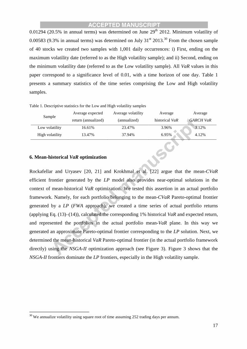
5. Sample descriptive statistics
For the purposes of this study, we selected 40 constituents of the S&P 100 with the highest
market capitalization as of Sept 6th
2013.29
We observed the constituents’ time series of 1,421
returns in the period Jan 15th
2008-Sept 6th
2013. We used a rolling window of 1,000 returns
for VaR estimation. For each day within the rolling estimation period of 421 days (Jan 4th
2012-Sept 6th
2013) we estimated 1-day ahead daily volatility of the S&P 100 time series. The
volatilities were estimated using the univariate GARCH (1, 1) model. Standardized returns
were assumed to have a standardized t-distribution. GARCH volatility estimations of the S&P
100 index were based on a rolling window of 1,000 daily returns. Maximum volatility of
28
We obtained these solutions and included them into the initial population of each MOEA execution. Maximum
return solution was obtained analytically, while minimum risk solution was obtained using single-objective
genetic algorithm. 29
Initially, 43 stocks were considered of which 3 were discarded (tickers: PM, V, KFT) due to incomplete data
during the sample period.
17
0.01294 (20.5% in annual terms) was determined on June 29th
2012. Minimum volatility of
0.00583 (9.3% in annual terms) was determined on July 31st 2013.
30 From the chosen sample
of 40 stocks we created two samples with 1,001 daily occurrences: i) First, ending on the
maximum volatility date (referred to as the High volatility sample); and ii) Second, ending on
the minimum volatility date (referred to as the Low volatility sample). All VaR values in this
paper correspond to a significance level of 0.01, with a time horizon of one day. Table 1
presents a summary statistics of the time series comprising the Low and High volatility
samples.
Table 1. Descriptive statistics for the Low and High volatility samples
Sample Average expected
return (annualized)
Average volatility
(annualized)
Average
historical VaR
Average
GARCH VaR
Low volatility 16.61% 23.47% 3.96% 3.12%
High volatility 13.47% 37.94% 6.95% 4.12%
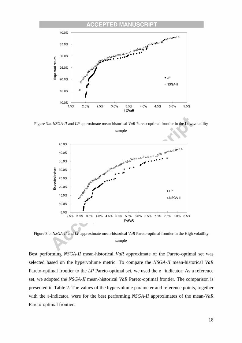
6. Mean-historical VaR optimization
Rockafellar and Uryasev [20, 21] and Krokhmal et al. [22] argue that the mean-CVaR
efficient frontier generated by the LP model also provides near-optimal solutions in the
context of mean-historical VaR optimization. We tested this assertion in an actual portfolio
framework. Namely, for each portfolio belonging to the mean-CVaR Pareto-optimal frontier
generated by a LP (FWA approach), we created a time series of actual portfolio returns
(applying Eq. (13)–(14)), calculated the corresponding 1% historical VaR and expected return,
and represented the portfolios in the actual portfolio mean-VaR plane. In this way we
generated an approximate Pareto-optimal frontier corresponding to the LP solution. Next, we
determined the mean-historical VaR Pareto-optimal frontier (in the actual portfolio framework
directly) using the NSGA-II optimization approach (see Figure 3). Figure 3 shows that the
NSGA-II frontiers dominate the LP frontiers, especially in the High volatility sample.
30
We annualize volatility using square root of time assuming 252 trading days per annum.
18
Figure 3.a. NSGA-II and LP approximate mean-historical VaR Pareto-optimal frontier in the Low volatility
sample
Figure 3.b. NSGA-II and LP approximate mean-historical VaR Pareto-optimal frontier in the High volatility
sample
Best performing NSGA-II mean-historical VaR approximate of the Pareto-optimal set was
selected based on the hypervolume metric. To compare the NSGA-II mean-historical VaR
Pareto-optimal frontier to the LP Pareto-optimal set, we used the ε –indicator. As a reference
set, we adopted the NSGA-II mean-historical VaR Pareto-optimal frontier. The comparison is
presented in Table 2. The values of the hypervolume parameter and reference points, together
with the ε-indicator, were for the best performing NSGA-II approximates of the mean-VaR
Pareto-optimal frontier.

19
Table 2. Comparison of NSGA-II mean-historical VaR and LP models
Sample Mutation
probability
Crossover
rate Hypervolume
Reference
point
ε-indicator
Low volatility 0.005 0.8 4.2366E-05 (0.0521,0) 1.1300
High volatility 0.05 1 6.9160E-05 (0.0823,0) 1.1526
The values for the ε-indicator confirm that the NSGA-II optimization approach provides better
mean-historical VaR trade-offs of actual portfolios compared to the LP solutions in both the
High and Low volatility samples. The relatively higher value of the ε-indicator (1.1526)
suggests that NSGA-II performed particularly well during the High volatility period.
7. Results for mean-GARCH VaR optimization
7.1. Pareto-optimal frontiers in the Low and High volatility samples
In this section we compared the Pareto-optimal frontiers for: i) The mean-univariate GARCH
VaR (or univariate GARCH for short); ii) The mean-multivariate GARCH VaR (benchmark 1);
and iii) The mean-historical VaR (benchmark 2).31
In order to obtain solutions in the actual
portfolio framework for both benchmark portfolio solutions (represented by the corresponding
vector of weights w), we generated a times series of portfolio returns. The time series of
portfolio returns was generated by employing Equations (13) and (14) within the APF
approach. We than calculated VaR using the univariate GARCH model (Eq. (4) and (5)).32
The results are shown in Figure 4. The Pareto-optimal frontiers, for actual portfolios, are for
the two volatility regimes when 1%VaR was estimated using the univariate GARCH model.
Triangle markers represent the univariate GARCH frontier (obtained via NSGA-II), while
filled dots represent benchmark 1 solutions and empty dots represent benchmark 2 solutions.
31
As presented in Figure 3, the NSGA-II method provided superior actual portfolio mean- historical VaR trade-
offs compared to the LP model, in both samples. Consequently, we adopted the NSGA-II mean-historical VaR
portfolios as benchmark 2. 32
During this process some of benchmark 1 and benchmark 2 portfolio solutions became dominated and thus
have been discarded from the approximation set.

20
Figure 4a. Pareto-optimal frontiers in the Low volatility sample
Figure 4b. Pareto-optimal frontiers in the High volatility sample
The differences are particularly prominent in the area of low returns (and low risk). In this
segment of the Pareto-optimal set, thus, the opportunities for improving the mean-VaR trade-
off through optimization are the greatest. It is worth noting that this segment of the Pareto-
optimal set is associated with most diversified portfolios. In contrast, with higher expected
return values, the cardinality of efficient portfolios is reduced (the highest return portfolio, by
construction, corresponds to a single asset).
To further compare the univariate GARCH Pareto-optimal frontier to the respective
benchmarks, we used the ε –indicator. As a reference set, we adopted the univariate GARCH

21
frontier. Table 3 presents the values of the hypervolume parameter and reference points for
the best performing NSGA-II mean-univariate GARCH VaR approximate Pareto-optimal sets.
The table also shows ε-indicators corresponding to the respective benchmarks in the Low and
High volatility samples.
Table 3. Parameters of the best performing mean-univariate GARCH VaR
Mutation
probability
Crossover
rate Hypervolume Reference
Point
ε-indicator
Benchmark 1 Benchmark 2
Low volatility 0.05 0.7 5.0973E-05 (0.0504, 0) 1.2608 1.4618
High volatility 0.01 0.9 5.3451E-05 (0.0581, 0) 1.0866 1.3243
The above presented ε-indicators confirm superiority of the univariate GARCH VaR
optimization approach. The advantages of the univariate GARCH VaR optimization approach
are particularly pronounced in the Low volatility sample. Measured by the ε-indicators, the
mean-historical VaR approach provides the worst approximations out of the three approaches.
The above result is particularly important given that approximately 75% of banks tend to use
the historical VaR models for portfolio optimization (see Pérignon and Smith [55]).
7.2. Process time (CPU time)
As expected, our CPU time is longer compared to the CPU time of the traditional methods
(e.g. QP). For example, the execution of one generation of NSGA-II, when solving the mean-
univariate GARCH VaR problem, lasted 41 seconds. Hence, to execute 1,000 generations of
NSGA-II we needed 41,000 seconds.33
The total CPU time for mean-univariate GARCH VaR
optimization with the QP solver was 424 seconds.34
Our additional analysis, however,
revealed that the NSGA-II CPU time could be shorter since the execution of 1,000 generations
was not always necessary. For example, for the mean-historical VaR optimization, 99% of
final hypervolume was achieved after 50 generations (12 seconds) in the Low volatility
sample, and after 52 generations (12.5 seconds) in the High volatility sample.35
The same
33
In comparison, it took only 1 second for the LP model to generate mean-historical VaR Pareto-optimal frontier
consisting of 100 solutions. 34
The mean-univariate GARCH VaR optimization (using multivariate GARCH VaR approach) consisted of three
steps: i) Determination of conditional variance-covariance matrix of individual returns (HT+1); ii) Execution of
QP solver; and iii) Estimation of univariate GARCH VaR for each solution obtained by using QP solver. To
determine conditional variance covariance matrix 382 seconds was needed. The execution of QP solver for
Pareto optimal front of 100 solutions lasted 1 second. Finally the estimation of univariate GARCH VaR, for 100
solutions obtained by using QP solver, lasted 41 second. 35
We define final hypervolume as a hypervolume of Pareto-optimal set generated after 1,000 generations.

22
analysis applied on the mean-univariate GARCH VaR optimization revealed that 99% of final
hypervolume was achieved after 40 generations (1,640 seconds) in the Low volatility sample.
The corresponding values in the High volatility sample were 20 generations and 820 seconds.
Given its longer CPU time, the use of NSGA-II could be justified by its greater flexibility and
ability to deal with more complex real-life portfolio optimization problems compared to the
QP method (see Deb et al. [35]).
7.3. Out-of-sample estimates
Bank managers and regulators are interested in the out-of-sample performance of different
optimization models. Thus, we compared out-of-sample performance of the different
optimization models used in our study. The optimization dates for our High and Low
volatility samples were dates with the highest (29th
June 2012) and lowest (31st July 2013)
volatilities. Based on the estimated portfolios on the optimization dates, we calculated
respective mean and VaR values for dates which fall exactly 1 month later (30th
July 2012 and
3rd
September 2013 respectively).
Figure 5a. Out-of-sample test in the High volatility sample
5.0%
10.0%
15.0%
20.0%
25.0%
30.0%
35.0%
40.0%
45.0%
1.5% 2.0% 2.5% 3.0% 3.5% 4.0% 4.5% 5.0% 5.5% 6.0% 6.5% 7.0%
Exp
ecte
d r
etu
rn
1%VaR
mean-univariate GARCH VaR
mean-multivariate GARCH VaR
mean-historical VaR
23
Figure 5b. Out-of-sample test in the Low volatility sample
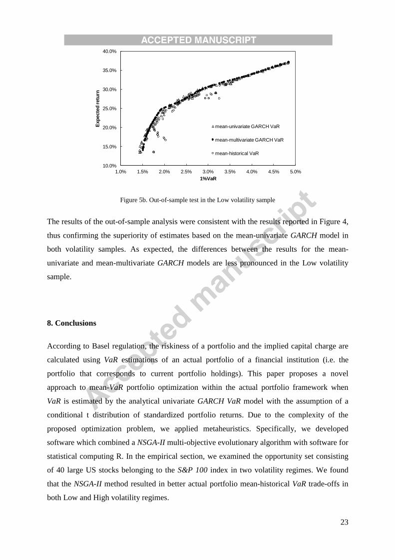
The results of the out-of-sample analysis were consistent with the results reported in Figure 4,
thus confirming the superiority of estimates based on the mean-univariate GARCH model in
both volatility samples. As expected, the differences between the results for the mean-
univariate and mean-multivariate GARCH models are less pronounced in the Low volatility
sample.
8. Conclusions
According to Basel regulation, the riskiness of a portfolio and the implied capital charge are
calculated using VaR estimations of an actual portfolio of a financial institution (i.e. the
portfolio that corresponds to current portfolio holdings). This paper proposes a novel
approach to mean-VaR portfolio optimization within the actual portfolio framework when
VaR is estimated by the analytical univariate GARCH VaR model with the assumption of a
conditional t distribution of standardized portfolio returns. Due to the complexity of the
proposed optimization problem, we applied metaheuristics. Specifically, we developed
software which combined a NSGA-II multi-objective evolutionary algorithm with software for
statistical computing R. In the empirical section, we examined the opportunity set consisting
of 40 large US stocks belonging to the S&P 100 index in two volatility regimes. We found
that the NSGA-II method resulted in better actual portfolio mean-historical VaR trade-offs in
both Low and High volatility regimes.
10.0%
15.0%
20.0%
25.0%
30.0%
35.0%
40.0%
1.0% 1.5% 2.0% 2.5% 3.0% 3.5% 4.0% 4.5% 5.0%
Exp
ecte
d r
etu
rn
1%VaR
mean-univariate GARCH VaR
mean-multivariate GARCH VaR
mean-historical VaR

24
Next, we compared the mean-univariate GARCH VaR Pareto-optimal frontier to the mean-
multivariate GARCH VaR and to the mean-historical VaR Pareto-optimal frontiers. In
comparison to the two benchmarks, the proposed univariate GARCH VaR procedure, again,
provided actual portfolios with a superior mean-univariate VaR frontier for both volatility
samples. The results suggest that the multivariate GARCH modeling framework lacks
flexibility to conform to the actual portfolio framework which is inherent in regulation. At the
same time, the mean-historical VaR frontier provided the worst mean-univariate GARCH VaR
trade-offs. Overall, our results bear two important implications for financial institutions and
their regulators. First, the results highlighted differences between the actual portfolio
approach and the approach based on the fixed weights. Second, the results show the
importance of carefully selecting amongst different VaR methodologies used in portfolio
optimization.
Recently, some multiple criteria decision making (MCDM) tools were combined with NSGA-
III to either rank or reduce the Pareto optimal frontier (see Tavana et al. [56]). Further
enhancement of our optimization approach with some of the MCDM reduction techniques
could be an interesting area for future research.
Acknowledgements: We would like to thank two anonymous referees for their helpful
suggestions. Research presented in this paper was supported by Serbian Ministry of
Education, Science and Technology, Grants OH 179005 and III-44010.

25
References
[1] Artzner P, Delbaen F, Eber JM, Heath D. Coherent measures of risk.
Mathematical Finance 1999; 9(3): 203–228.
[2] Szego G. Measures of risk. Journal of Banking & Finance 2002; 26: 1253–1272.
[3] Basel Committee on Banking Supervision. International convergence of capital
measurement and capital standards. Bank for International Settlements (BIS);
1988.
[4] Basel Committee on Banking Supervision. Amendment to the capital accord to
incorporate market risks. Bank for International Settlements (BIS); 1996.
[5] Basel Committee on Banking Supervision. Revisions to the Basel II market risk
framework. Bank for International Settlements (BIS); 2009.
[6] Hendricks D, Hirtle B. Bank capital requirements for market risk: the internal
models approach. Economic Policy Review 1997; 3: 1–12.
[7] Engle R. Autoregressive conditional heteroscedasticity with estimates of the
variance of UK inflation. Econometrica 1982; 50(4): 987-1007.
[8] Bollerslev T. Generalized autoregressive conditional heteroscedasticity. Journal of
Econometrics 1986; 31: 307-327.
[9] Christoffersen PF. Elements of Financial Risk Management. 2nd
ed. San Diego
CA: Academic Press; 2012.
[10] Huisman R, Koedijk K, Pownall R. VaR-x: Fat tails in financial risk management.
Journal of Risk 1998; 1: 47–61.
[11] Alexander C. Value-at-Risk Models. 1th ed. England: John Wiley & Sons; 2008b.
[12] Alexander C, Sheedy E. Developing a stress testing framework based on market
risk models. Journal of Banking & Finance 2008; 32: 2220–2236.
[13] Berkowitz J, O’Brien J. How accurate are value-at-risk models at commercial
banks? Journal of Finance 2002; 57: 1093–1111.
[14] Hull J, White A. Incorporating volatility updating into the historical simulation
method for value at risk. Journal of Risk 1998; 1: 5-19.
[15] Pritsker M. The hidden dangers of historical simulation, Journal of Banking &
Finance 2006; 30: 561–582.
[16] Gaivoronski AA, Pflug G. Value-at-risk in portfolio optimization: properties and
computational approach. Journal of Risk 2005; 7(2): 1-31.

26
[17] Goh JW, Guan LK, Sim, M, Zhang W. Portfolio value-at-risk optimization for
asymmetrically distributed asset returns. European Journal of Operational
Research 2012; 221: 397–406.
[18] Krejić N, Kumaresan M, Rožnjik A. VaR optimal portfolio with transaction costs.
Applied Mathematics and Computation 2011; 218: 4626-4637.
[19] Natarajan K, Pachamanova D, Sim M. Incorporating asymmetric distributional
information in robust value-at-risk optimization. Management Science 2008;
54(3): 573-585.
[20] Rockafellar RT, Uryasev S. Optimization of conditional value-at-risk. Journal of
Risk 2000; 2(3): 21–41.
[21] Rockafellar RT, Uryasev S. Conditional value-at-risk for general loss
distributions. Journal of Banking & Finance 2002; 26: 1443–1471.
[22] Krokhmal P, Palmquist J, Uryasev S. Portfolio optimization with conditional
value-at-risk objective and constraints. Journal of Risk 2002; 4(2): 11-27.
[23] Iscoe I, Kreinin A, Mausser H, Romanko O. Portfolio credit-risk optimization,
Journal of Banking & Finance 2012; 36: 1604–1615.
[24] Pfaff B. Financial risk modelling and portfolio optimization with R. UK: John
Wiley & Sons; 2013.
[25] Würtz D, Chalabi Y, Chen W, Ellis A. Portfolio optimization with R/Rmetrics.
Rmetrics; 2009.
[26] Santos A, Francisco J, Nogales ER, Dick VD. Optimal portfolios with minimum
capital requirements. Journal of Banking & Finance 2012; 36: 1928–1942.
[27] Metaxiotis K, Liagkouras K. Multi-objective evolutionary algorithms for portfolio
management: a comprehensive literature review. Journal of Expert Systems with
Applications: An International Review 2012; 39 (14): 11685-11698.
[28] Schlottmann F, Seese D. Financial applications of multi-objective evolutionary
algorithms: Recent development and future research directions. In: Coello-Coello
C, Lamont G. editors. Applications of Multi-objective Evolutionary Algorithms.
World Scientific; 2004, p. 627-652.
[29] Tapia MGC, Coello CAC. Applications of multi-objective evolutionary
algorithms in economics and finance. In: IEEE Congress on Evolutionary
Computation; 2007, p. 532–539.
[30] Ponsich A, L´opez J A, Coello CAC. A Survey on multiobjective evolutionary
algorithms for the solution of the portfolio optimization problem and other finance

27
and economics applications, IEEE Transactions on Evolutionary Computation
2013; 17 (3): 321-344.
[31] Anagnostopoulos KP, Mamanis G. The mean-variance cardinality portfolio
optimization problem: An experimental evaluation of five multi-objective
evolutionary algorithms, Expert Systems with Applications 2011; 38: 14208–
14217.
[32] Anagnostopoulos KP, Mamanis G. Multiobjective evolutionary algorithms for
complex portfolio optimization problems, Computational Management Science
2011; 8: 259–279.
[33] Anagnostopoulos KP, Mamanis G. A portfolio optimization model with three
objectives and discrete variables. Computers & Operations Research 2010; 37:
1285–1297.
[34] Deb K, Agrawal S, Pratap A, Meyarivan TA. A fast elitist non-dominated sorting
genetic algorithm for multi-objective optimization: NSGA-II. Lecture Notes in
Computer Science 2000; 1917: 849-858.
[35] Deb K, Steuer RE, Tewari R, Tewari R. Bi-objective portfolio optimization using
a customized hybrid NSGA-II procedure. In: Takahashi RHC, Deb K, Wanner EF,
Greco S. editors. EMO 2011. Lecture Notes in Computer Science 6576. Berlin:
Springer-Verlag; 2011, p. 358–373.
[36] Branke J, Scheckenbach B, Stein M, Deb K, Schmeck H. Portfolio optimization
with an envelope-based multi-objective evolutionary algorithm. European Journal
of Operational Research 2009; 199: 684–693.
[37] Deb K, Pratap A, Agarwal S, Meyarivan, TA. Fast and elitist multi-objective
genetic algorithm: NSGA-II. IEEE Transactions on Evolutionary Computation
2002; 6(2):182–197.
[38] Deb K, Jain H. An evolutionary many-objective optimization algorithm using
reference-point-based nondominated sorting approach, part 1: solving problems
with box constraints. IEEE Transactions on Evolutionary Computation 2014;
18(4): 577-601.
[39] Jain H, Deb K. An evolutionary many-objective optimization algorithm using
reference-point based non-dominated sorting approach, part 2: handling
constraints and extending to an adaptive approach. IEEE Transactions on
Evolutionary Computation 2014; 18(4): 602-622.

28
[40] Mobin M, Li Z, Khoraskani M. Multi-objective X-bar control chart design by
integrating NSGA-II and data envelopment analysis. In: Proceedings of the
Industrial and Systems Engineering Research Conference (ISERC), TN, USA;
2015.
[41] Hochreiter R. An evolutionary computation approach to scenario risk-return
portfolio optimization for general risk measures. Department of Statistics and
Decision Support Systems-University of Vienna, 2007.
[42] Soler JS, Cid EA, Blanco MO. Mean-VaR portfolio selection under real
constraints. Comput. Econ 2011; 37:113-131.
[43] Ranković V, Drenovak M, Stojanović B, Kalinić Z, Arsovski Z. The mean-value-
at-risk static portfolio optimization using genetic algorithm. Computer Science
and Information Systems 2014; 11 (1): 89–109.
[44] Alexander C. Practical Financial Econometrics. England: John Wiley & Sons;
2008.
[45] Engle RF, Kroner KF. Multivariate simultaneous generalized ARCH.
Econometric Theory 1995; 11:122-150.
[46] Alexander C. Quantitative methods in finance. England: John Wiley & Sons;
2008.
[47] Engle R. Dynamic conditional correlation: a simple class of multivariate
generalized autoregressive conditional heteroskedasticity models. Journal of
Business & Economic Statistics 2002; 20: 339–350.
[48] Ghalanos A. rmgarch: Multivariate GARCH models. R package version 1.2-8;
2014.
[49] R Core Team. R: A language and environment for statistical computing. R
Foundation for Statistical Computing 2014. Vienna: URL http://www.R-
project.org/.
[50] Markowitz HM. Portfolio selection. Journal of Finance 1952; 7: 77–91.
[51] Sastry K, Goldberg D, Kendall G. Genetic algorithms. In: Edmund KB, Graham
K. editors. Search methodologies: Introductory tutorials in optimization and
decision support techniques. New York: Springer Science+Business Media; 2005,
p. 97-127.
[52] Coello CAC, Lamont GB, Van Veldhuizen DA. Evolutionary algorithms for
solving multi-objective problems. 2nd
ed. Berlin: Springer; 2007.
29
[53] Zitzler E, Thiele L, Laumanns M, Fonseca CM, Grunert da Fonseca V.
Performance assessment of multi-objective optimizers: an analysis and review.
IEEE Transactions on Evolutionary Computation 2003; 7: 117–32.
[54] Ghalanos A. rugarch: Univariate GARCH models. R package version 1.3-3; 2014.
[55] Pérignon C, Smith D. The Level and quality of value-at-risk disclosure by
commercial banks, Working paper - Simon Fraser University, 2007.
[56] Tavana, M., Li, Z., Mobin, M., Komaki, M., Teymourian, E. Multi-objective
control chart design optimization using NSGA-III and MOPSO enhanced with
DEA and TOPSIS. Expert Systems with Applications 2016; 50; 17-39.

30
Appendix
Table A1: Acronyms
APF Actual Portfolio Framework
CPU Time Process Time
CR Capital Requirements
CVaR Conditional Value-at-Risk
DCC Dynamic Conditional Correlation Model
EA Evolutionary Algorithm
ES Expected Shortfall
FWA Fixed Weights Approach
GARCH Generalized AutoRegressive Conditional Heteroscedasticity
LP Linear Programming
MCDM Multiple Criteria Decision Making
MLE Maximum Likelihood Estimation
MOEA Multi-objective Evolutionary Algorithm
NSGA-II (NSGA-III) Nondominated Sorting Genetic Algorithm
PESA Pareto Envelope-based Selection Algorithm
PAES Pareto Archived Evolutionary Strategy
QP Quadratic Programming
S&P 100 Standard and Poor’s 100 stock market index
SPEA Strength Pareto Evolutionary Algorithm
VaR Value-at-Risk

31
Table A2: Notations
rt Portfolio return
μt Conditional expected return
σt2 Conditional variance
zt Residual (innovation) term
p Portfolio
ρ Probability
Vp,t Dollar portfolio value
σt+1 1-day ahead conditional volatility
F(α) Cumulative distribution function of returns
α Significance level
h Time horizon
d Degrees of freedom
Ht+1 1-day ahead conditional variance-covariance matrix of returns
wt Vector of portfolio weights
GARCH VaR of a portfolio
E(r) Portfolio expected return
Pi,t Company i share price
ni Portfolio holdings