Mean height and variability of height derived from lidar...

SilviLaser 2008, Sept. 17-19, 2008 – Edinburgh, UK

517

Mean height and variability of height derived from lidar data and Landsat images relationship

Cristina Pascual1, Warren Cohen2, Antonio García-Abril1, Lara A. Arroyo3, Rubén

Valbuena1, Susana Martí-Fernández1 and José Antonio Manzanera1

1Technical University of Madrid (UPM), E.T.S.I Montes, Ciudad Universitaria s.n., 28040 Madrid, Spain. [email protected]

2Forestry Sciences Laboratory, Pacific Northwest Research Station, USDA Forest Service, 3200 SW Jefferson Way, Corvallis, OR 97311, USA

3Centre for Remote Sensing and Spatial Information Science, School of Geography, Planning and Architecture, University of Queensland, Brisbane, QLD 4072, Australia.

Abstract The mean and standard deviation of lidar-derived height data have shown to be important variables with which to summarize forest structure. However, lidar data has a limited spatial extent and a very high economic cost. Landsat data provides useful structural information in the horizontal plane and is easily accessible. The integration of both data sources offers an interesting opportunity to aid sustainable forest management. Different spectral indices (NDVI and Tasseled Cap) were obtained from three Landsat scenes (March 2000, June 2001 and September 2001), and the mean and standard deviation of lidar height measurements were calculated in 30 m square blocks. Correlation and forward stepwise regression analysis was applied to these data sets. Mean lidar height versus NDVI and wetness Tasseled Cap showed the best correlation coefficients (ranging between 0.65 and -0.73). The best regression models included NDVI and wetness for June and September as dependent variables (adjusted r2: 0.55 – 0.62). These results showed that lidar data can be used to train Landsat to map forest structure, and it should be interesting to further optimize this approach. Keywords: lidar, Landsat, mean height, forest structure 1. Introduction Canopy structure can be defined as the organization in space and time, including the position, extent, quantity, type and connectivity, of the aboveground components of vegetation (Parker, 1995; Lefsky et al., 1999). Structure includes vertical (e.g. number of tree layers, understory vegetation) and horizontal features (e.g. spatial pattern of trees, gaps) as well as species richness (Maltamo et al., 2005). The mean and standard deviation of lidar-derived height data have shown to be variables that synthesise forest structure of the canopy. Zimble et al. (2003) used lidar-derived tree height variances to distinguish between single-story and multi-story forest classes. Lefsky et al. (2005a) pointed out that mean height and height variability figures derived from lidar data are strongly related to canopy indices and thus related to stand structure. These authors consider these variables to represent the same kind of enhancement of lidar data that the Tasselled Cap indices represent for optical remote sensing. Pascual et al. (2008) found that mean, median and standard deviation of height derived from lidar could be used to distinguish horizontally heterogeneous forest structure types.


518

Small footprint airborne laser scanners provide detailed information on the vertical distribution of forest canopy structure (Hyyppa et al., 2008), but over a limited spatial extent and with a high economic cost. Landsat data provides useful structural information in the horizontal plane and is much more accessible (Cohen & Spies, 1992). Therefore the integration of optical remote sensing imagery and lidar data provides improved opportunities to fully characterize forest canopy attributes and dynamics (Wulder et al., 2007). Hudak et al. (2002) developed spatial extrapolation of lidar data over Landsat images. Methods for the combination of lidar-derived metrics and optical images has been also devised (Chen et al., 2004; Lefsky et al., 2005b). In addition, two coincident lidar transects, representing 1997 and 2002 forest conditions in the boreal forest of Canada, were compared using image segments generated from Landsat ETM+ imagery (Wulder et al., 2007). Given the relationship between mean and standard deviation of height derived from lidar and forest structure, the objective of the present work is to evaluate the relationship between summaries derived from lidar and spectral information from the Landsat satellite. The final aim of this work is to establish whether Landsat data can be used to predict lidar forest canopy height (mean and standard deviation). 2. Methods 2.1 Study area A 127.10 ha (1293 x 983 m) area, located on the western slopes of the Fuenfría Valley (40º 45´N, 4º 5´ W) in central Spain, was selected as the study area. The Fuenfría Valley is located in the northwest portion of the Madrid region (Figure 1). The predominant forest is Scots pine (Pinus sylvestris, L.) with abundant shrubs (Cytisus scoparious (L.) Link., C. oromediterraneus Rivas Mart. et al., Genistaflorida (L.)) in some areas.

Figure 1: Study site. Fuenfría Valley, in the village of Cercedilla, northwest of Madrid (Spain).

There are small pastures on the lowest part of the hillside. In the northern sector of the study site there is an extensive rocky area. The site has a mean annual temperature of 9.4ºC and precipitation averages 1180 mm per year. Elevations range between 1310 m and 1790 m above sea level, with slopes between 20% and 45%. The general aspect of the study site is east.


519

2.2. Lidar data A small footprint lidar dataset was acquired by TopoSys GmbH over the study area in August, 2002. The TopoSys II lidar system recorded first and last returns with a footprint diameter of 0.95 m. Average point density was 5 points m-2. The raw data (x, y, z-coordinates) was processed into two digital elevation models by TopoSys using the company’s proprietary software. The digital surface model (DSM) was processed using the first pulse backscatters and the digital terrain model (DTM) was constructed from the last returns. Filtering algorithms were used to identify canopy and ground surface returns for an output pixel resolution of 1 m horizontally and 0.1 m vertically. According to TopoSys calculations the DSM and DTM positional accuracy was 0.5 m horizontally and 0.15 m vertically. To obtain a digital canopy height model (DCHM), the DTM was subtracted from the DSM. Both the DTM and DCHM were validated before use by land surveying with a total station and ground-based tree height measurements. The vertical accuracies, calculated as Root Mean Square Error (RMSE) obtained for the DTM in open areas and the DCHM under forest canopy were 0.30 m and 1.3 m, respectively (Pascual, 2006). These accuracies were acceptable for this study, and were in agreement with previous studies. For example, Clark et al. (2004) reported RMSEs for DTMs ranging from 0.06 to 0.61 m and for DCHMs ranging from 0.23 m to 2.41 m in tropical landscapes. 2.2. Image data and preprocessing In this study we used three Landsat ETM+ images from scene path/row (201/32) corresponding to three different dates (March 15th, 2000, June 6th, 2001 and September 10th, 2001). The Landsat images were georeferenced and radiometrically calibrated.

June and September’s Landsat images were co-registered, at the Alcalá University’s Geography Department, using digital highway maps of the Madrid region (E 1:50.000). RMSE was less than 30 m (1 pixel); the projection system was UTM (Datum Europeo 1950) with a pixel resolution of 30 m. We validated the image co-registration in the study area using a set of easily recognisable points.

From the March Landsat image, a subset area of 30 x 30 km was orthorectified. Control points were selected, taking as reference September’s georeferenced image. The source of altitudinal information was a 20 m pixel DTM of the Madrid region. We used 38 control points, homogenously spread out over the subset image. RMSE was 11.49 m (0.4 pixels). The COST absolute radiometric correction model of Chavez (1996) was applied to each image to convert digital counts to reflectance.

2.3. Lidar DCHM summaries (mean and standard deviation) and spectral indices The DCHM lidar (1 m pixel) was degraded to 30 m cell blocks, providing a 30 m grid of 32 rows and 41 columns. The mean and standard deviation of the 900 lidar height values contained in each 30 x 30 m block were calculated. Two new 30 m pixel images of the mean and standard deviation of lidar height values were thus obtained. NDVI and Tasseled Cap (TCAP) were calculated for the March, June and September Landsat images. TCAP transformation was obtained using coefficients for brightness, greenness and wetness derived by Crist (1985). According to Cohen et al. (2003), no published transformation exists to convert atmospherically-corrected ETM+ spectral data into Tasseled Cap indices. However, the authors have verified that Landsat TM and ETM+ are similar enough to assume


520

that any differences in Tasseled Cap indices derived from data from the two different sensors are minor. 2.4. Sample design and statistical analysis First, we created a mask to exclude bare soil, rocks, pasture and shrubs from subsequent analysis (Figure 2) performing unsupervised classification of the September Landsat image. In addition, systematic sampling was used to reduce the spatial autocorrelation inherent in remote sensing imagery. The sampling procedure was designed based on semivariograms of the lidar DCHM mean height and wetness Tasseled component. Semivariograms were calculated using the free distribution software Variowin 2.2. (Pannatier, 1996). Mean lidar height was selected based on previous work (Pascual, 2006) and wetness TCAP component because is often related to forest structure (Cohen & Spies, 1992). The semivariance tends to stability at 130-150 m. Therefore, two samples were obtained, each using one out of every four or five pixels, one for statistical model building and the other to independently validate the model.

Figure 2: 0.5 m pixel digital orthophoto of the study area (yellow frame). Different covertures (pasture,

bare soil, shrubs and Populus sp) were digitalised and labelled. Pearson’s correlation among Landsat spectral indices and lidar statistical descriptors was performed. Furthermore, forward step regression analysis (p enter = 0.05; p remove = 0.05) was carried out between both variable sets. All statistical analysis was conducted using STATISTICA 6.1 software. Before proceeding with regression analysis, the normality of the dependent and independent variables was verified and transformed when needed.

Populus sp

Pasture

Bare soil shrubs


521

3. Results and Discussion Mean lidar height and standard deviation of lidar height provided two images (Figure 3) with a gradient from black to white representing spatial variation in canopy height.

Figure 3: Mean lidar height image (30m pixel) (left) and Standard deviation of lidar height (right). Black to white gradient represent growing height values. Vectorial digitized covertures are included.

Correlations among NDVI indexes (Figure 4) and the square root of mean lidar height ( hmean ) indicated a moderately strong relationship among these variables (r = 0.65, r = 0.70 y r = 68; p = 0.05; n = 47 for March, June and September respectively). Standard deviation of lidar height (sd_30) demonstrated an insignificant relationship with all NDVI indices for the three dates (Table 1).

Table 1: Pearson’s correlation between lidar-derived metrics and spectral indices (n = 47). March 15th

NDVI Br Gr We hmean 0.65* -0.50* 0.46* 0.64* sd_30 0.20 -0.16 0.18 0.20

June 6th NDVI 1/Br Gr Log(-We)

hmean 0.70* 0.65* 0.50* -0.72* sd_30 0.30* 0.13 0.26 -0.11

September 10th NDVI 1/Br Gr Log(-We)

hmean 0.68* 0.59* 0.34* -0.73* sd_30 0.29* 0.15 0.17 -0.04

*significant correlations p < 0.05; Br, Gr and We are brightness, greenness and wetness Tasseled components derived from ETM+.

Lu et al. (2004) found strong correlations between NDVI and forest attributes derived from field measurements. Nevertheless, Hall et al. (1995) and Franklin et al. (1997) do not consider this spectral index especially appropriate for the study of forest attributes because of the weak correlation that has been shown with certain parameters of vegetation. Regarding this, Lu et al. (2004) indicate that conclusions as to its application vary depending on the biophysical parameters and the characteristics of the study area.


522

a)

b)

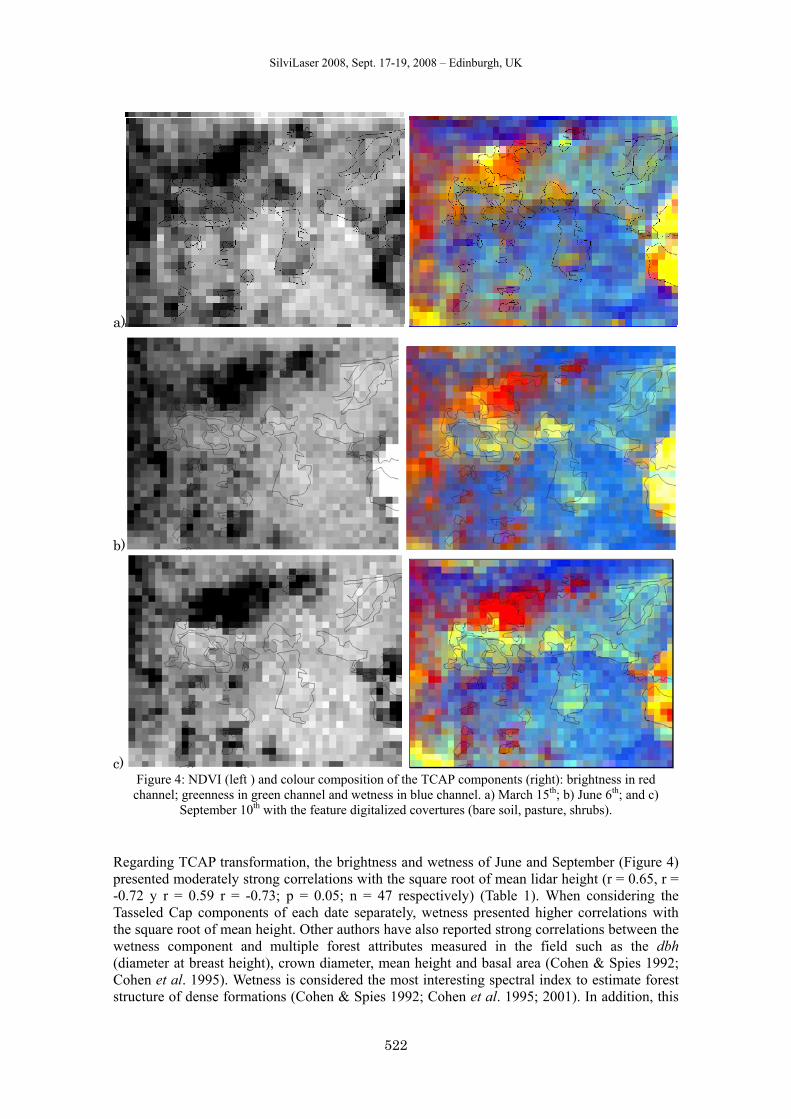
c) Figure 4: NDVI (left ) and colour composition of the TCAP components (right): brightness in red channel; greenness in green channel and wetness in blue channel. a) March 15th; b) June 6th; and c)

September 10th with the feature digitalized covertures (bare soil, pasture, shrubs).

Regarding TCAP transformation, the brightness and wetness of June and September (Figure 4) presented moderately strong correlations with the square root of mean lidar height (r = 0.65, r = -0.72 y r = 0.59 r = -0.73; p = 0.05; n = 47 respectively) (Table 1). When considering the Tasseled Cap components of each date separately, wetness presented higher correlations with the square root of mean height. Other authors have also reported strong correlations between the wetness component and multiple forest attributes measured in the field such as the dbh (diameter at breast height), crown diameter, mean height and basal area (Cohen & Spies 1992; Cohen et al. 1995). Wetness is considered the most interesting spectral index to estimate forest structure of dense formations (Cohen & Spies 1992; Cohen et al. 1995; 2001). In addition, this


523

component has been revealed as most significant when studying the temporal evolution of forests, such as mortality (Collins & Woodcok, 1994), harvesting and silvicultural activities (Wilson & Sader, 2002; Healey et al., 2005) or in the evaluation of damage by plagues (Skakun, et al., 2003). Standard deviation of lidar height (sd_30) and Tasseled components revealed weak and not significant correlations (Table 1). Regarding regression analysis (Table 2), the three models presented coefficients of determination ranging from 0.55 to 0.63. Standard deviation of height derived from lidar (SD_30) was excluded from regression analysis due to low Pearson´s correlation (Table 1). None of the three models presented colinearity problems (i.e. linear relationship among the independent variables problems). The variance inflation factor (VIF), as indicator of multicolinearity, did not present any variable values close to 5 or 10. According to Montgomery, et al. (2002) those are the thresholds that question regression coefficients estimated by minimum squares.

Table 2: Forward stepwise regression models

Name Models (forward stepwise regression) r2 adjusted RMSE

Mod. NDVI

junNDVImarNDVIhmean _0085.0_0043.0137.1 ⋅+⋅−= 0.55 4.07

Mod. TCAP

)_(907.0_133.0970.3 sepWeLogmarGrhmean −⋅−⋅+= 0.62 4.58

Mod. Mixed

junNDVIsepWeLoghmean _140.0)_(666.0832.2 ⋅+−⋅−= 0.59 4.32

A validation of regression analysis was performed using an independent sample of 54 pixels. Observed versus predicted values were represented in scatterplot graphs (Figure 5). All models showed a moderately strong adjustment (r = 0.73, p = 0.000; r = 0.72, p = 0.000 y r = 0.79, p = 0.000, n = 54 for Mod. NDVI, TCAP and MIXED respectively). Based on validation results, the best regression models were Mod. NDVI and Mod. MIXED.

Observed vs. PredictedMod. NDVI

1.5 2.0 2.5 3.0 3.5 4.0 4.5

Valores observados

1.5

2.0

2.5

3.0

3.5

4.0

4.5

Val

ores

pre

dich

os

r2 = 0.523; r = 0.726; p = 0.0000 y = 0.954 + 0.682 x

Observ ed v s. PredictedMod TCAP

1.5 2.0 2.5 3.0 3.5 4.0 4.5

Valores observados

1.5

2.0

2.5

3.0

3.5

4.0

4.5

Valo

res

pred

icho

s

r2 = 0.525; r = 0.723; p = 0.0000 y = 1.043 + 0.639 x

Observ ed v s. PredictedMod. MIXTED

1.5 2.0 2.5 3.0 3.5 4.0 4.5

Valores observados

1.5

2.0

2.5

3.0

3.5

4.0

4.5

Valo

res

pred

icho

s

r2 = 0.615; r = 0.785; p = 0.0000 y = 0.922 + 0.682 x

Figure 5. Scatterplots of independent (n=54) validation regression models (observed vs. predicted). Left (Mod. NDVI); middle (Mod. TCAP) and right (Mod. MIXED). Conclusions Mean lidar height derived from lidar for a Scot pine forest in Cercedilla was estimated through a combination of spectral indices derived from Landsat images. Wetness TCAP component showed higher correlations with square root of mean height derived from lidar. A wetness


524

relationship with forest structure has been reported by different authors. Regression models were explicative, because of the relationships among variables. Nevertheless regression models presented high variability (r2: 0.55 – 0.62) that diminished their predictive capacity. These results show that lidar data can be useful for training Landsat to map mean height. Given the relationship between mean lidar height derived from lidar and the forest structure, Landsat data can help to characterize forest structure. This approach should be analyzed in future research. References Chavez, P., 1996. Image-based atmospheric corrections—Revisited and improved.

Photogrammetric Engineering and Remote Sensing, 62, 1025–1036. Chen, X., Vierlinga, L., Rowell, E. and DeFelice, T., 2004,. Using lidar and effective LAI data

to evaluate IKONOS and Landsat 7 ETM+ vegetation cover estimates in a ponderosa pine forest. Remote Sensing of Environment, 91, 14–26.

Clark, M.L., Clark, D.B. and Roberts, D.A., 2004. Small-footprint lidar estimation of sub-canopy elevation and tree heigth in a tropical rain forest landscape. Remote Sensing of Environment, 91, 68 - 89.

Cohen, W. B. and Spies, T. A., 1992. Estimating structural attributes of Douglas-Fir western Hemlock forest stands from Landsat and SPOT imagery. Remote Sensing of Environment, 41, 1-17.

Cohen, W. B., Spies, T. A. and Fiorella, M., 1995. Estimating the age and structure of forests in a multi-ownership landscape of western Oregon, U.S.A. International Journal of Remote Sensing, 16, 721–746.

Cohen, W. B., Maiersperger, T. K., Spies, T. A. and Oetter, D. R., 2001. Modeling forest cover attributes as continuous variables in a regional context with Thematic Mapper data. International Journal of Remote Sensing, 22, 2279–2310.

Collins, J. B. and Woodcock, C. E., 1994. Change detection using the Gramm–Schmidt transformation applied to mapping forest mortality. Remote Sensing of Environment, 50, 267–279.

Crist, E. P., 1985. A TM tasseled cap equivalent transformation for reflectance factor data. Remote Sensing of Environment, 17, 301– 306.

Franklin, S. E., Lavigne, M. B., Deuling, M. J., Wulder, M. A. and Hunt Jr., E. R., 1997. Estimation of forest leaf area index using remote-sensing and GIS data for modeling net primary production. International Journal of Remote Sensing, 18, 3459–3471.

Hall, F. G., Shimabukuro, Y. E. and Huemmrich, K. F., 1995. Remote sensing of biophysical structure using mixture decomposition and geometric reflectance models. Ecology Applications, 5, 993-1013.

Healey, S. P., Cohen, W. B., Zhiqiang, Y. and Krankina, O. N., 2005. Comparison of Tasseled Cap-based Landsat data structures for use in forest disturbance detection. Remote Sensing of Environment, 97, 301-310.

Hudak, A. T., Lefsky, M. A., Cohen, W. B. and Berterretche, M., 2002. Integration of LiDAR and Landsat ETM+ data for estimating and mapping forest canopy height. Remote Sensing of Environment, 82, 397–416.

Hyyppa, J., Hyyppa, H., Leckie, D., Gougeon, F., Yu, S. and Maltamo, M., 2008. Review of methods of small-footprint airborne laser scanning for extracting forest inventory data in boreal forests. International Journal of Remote Sensing, 29, 1339-1366.

Lefsky, M. A., Cohen, W. B., Acker, S. A., Parker, G. G., Spies T. A. and Harding, D., 1999. Lidar remote sensing of the canopy structure and biophysical properties of Douglas-Fir


525

Western Hemlock forests. Remote Sensing of Environment, 70, 339-361 Lefsky, M. A., Hudak, A. T., Cohen, W. B. and Acker, S. A.,. 2005a. Patterns of covariance

between forest stand and canopy structure in the Pacific Northwest. Remote Sensing of Environment, 95, 517–531.

Lefsky, M. A., Turner, D. P., Guzy, M. and Cohen, W. B. ,2005b. Combining lidar estimates of aboveground biomass and Landsat estimates of stand age for spatially extensive validation of modelled forest productivity. Remote Sensing of Environment, 95, 549-558.

Lu, D., Mausel, P., Brondízio, E. and Moran, E., 2004. Relationship between forest stand parameters and Landsat TM spectral responses in the Brazilian Amazon Basin. Forest Ecology and Management, 198: 149-167.

Maltamo, M., Packalen, P., Yu, X., Eerikainen, K., Hyyppa, J., Pitkanen, J., 2005. Identifying and quantifying structural characteristics of heterogeneous boreal forests using laser scanner data. Forest Ecology and Management, 216, 41–50.

Montgomery, D., Peck, E. and Vining, G., 2002. Introducción al Análisis de Regresión Lineal. Compañía Editorial Continental. México.

Pannatier, Y. (1996). Variowin: Software for Spatial Data Analysis in 2D. Springer-Verlag. New York.

Parker, G. G..,1995. Structure and microclimate of forest canopies. In Forest Canopies—A Review of Research on a Biological Frontier (M. Lowman & N. Nadkarni, Eds.), Academic, San Diego, pp. 73–106.

Pascual, C., 2006. Análisis de la estructura forestal mediante teledetección: LiDAR (Light Detection And Ranging) e imágenes de satélite, Ph.D. thesis. Technical University of Madrid (UPM), Madrid.

Pascual, C., García-Abril, A., García-Montero, L.G., Martín-Fernández, S., Cohen, W.B.,2008. Object-based semi-automatic approach for forest structure characterization using lidar data in heterogeneous Pinus sylvestris stands. Forest Ecology and Management, 255, 3677-3685.

Skakun, R. S., Wulder, M. A. and Franklin, S. E., 2003. Sensitivity of the thematic mapper enhanced wetness difference index to detect mountain pine beetle red-attack damage. Remote Sensing of Environment, 86, 433-443.

Wilson, E. H. and Sader, S. A, 2002. Detection of forest harvest type using multiple dates of Landsat TM imagery. Remote Sensing of Environment, 80, 385– 396.

Wulder, M.A., Hana, T., White, J.C., Sweda, T. and Tsuzuki, H., 2007. Integrating profiling LIDAR with Landsat data for regional boreal forest canopy attribute estimation and change characterization. Remote Sensing of Environment, 110, 123-137

Zimble, D.A., Evans, D.L., Carlson, G.C., Parker, R.C., Grado, S.C. and Gerard, P.D., 2003. Characterizing vertical forest structure using small-footprint airborne LiDAR. Remote Sensing of Environment, 87, 171 - 182.

Mean height and variability of height derived from lidar...

Documents

Transcript of Mean height and variability of height derived from lidar...