MEAN FLOW AND TURBULENCE IN OPEN-CHANNEL BEND …€¦ · · 2011-01-01JOURNAL OF HYDRAULIC...

MEAN FLOW AND TURBULENCE IN OPEN-CHANNEL BEND

By Koen Blanckaert1 and Walter H. Graf,2 Member, ASCE

ABSTRACT: Flow over a developed bottom topography in a bend has been investigated experimentally. Themeasuring section is in the outer-bank half of the cross section at 607 into the bend. Spatial distributions of themean velocities, turbulent stresses, and mean-flow and turbulent kinetic energy are presented. The cross-sectionalmotion contains two cells of circulation: besides the classical helical motion (center-region cell), a weakercounterrotating cell (outer-bank cell) is observed in the corner formed by the outer bank and the water surface.The downstream velocity in the outer half-section is higher than the one in straight uniform flow; the core ofmaximum velocities is found close to the separation between both circulation cells, well below the water surface.The turbulence structure in a bend is different from that in a straight flow, most notably in a reduction of theturbulent activity toward the outer bank. Both the outer-bank cell and reduced turbulent activity have a protectiveeffect on the outer bank and the adjacent bottom and thus influence the stability of the flow perimeter and thebend morphology.

INTRODUCTION

Most natural rivers meander and tend to erode the outerbanks in their successive bends. Important engineering effortsare undertaken on rivers of all scales to stabilize the banklines.This is an essential component of projects to improve navi-gability; increase flood capacity and decrease floodplain de-struction; avoid massive loss of fertile soil (Odgaard 1984);and reduce dredging requirements of the river. Recently, therehas been an increased interest in the modeling of the erosionalbehavior of the outer bank (see the discussion section). How-ever, little is known about the characteristics of the mean flowand turbulence near the outer bank, where the flow pattern ishighly three-dimensional (3D).

A large amount of research on flow in bends has been per-formed in the last decades, but most of the experimental in-vestigations concentrated on the central portion of the flowand often did not cover the outer-bank region in detail. More-over, in most investigations a fixed rectangular section with asmooth bed was imposed on the flow. This is different fromthe rough turbulent flow over a typical developed bed topog-raphy, as found in nature. Furthermore, in most experimentalinvestigations, not all of the three velocity and six turbulentstress components were measured, and the measuring gridswere rather coarse. A literature review of experimental re-search on flow in open-channel bends is given in Table 1.

More recently, environmental problems such as the spread-ing and mixing of pollutants or the transport in suspension ofpolluted sediments have become of major concern in rivermanagement. These phenomena are closely related to the tur-bulence structure of the flow.

The scarcity of reliable experimental data on the 3D flowpattern and turbulence structure, particularly in bends, is re-sponsible for the lack of insight into the physical mechanisms,such as those related to outer-bank erosion and the mixing ofpollutants. Furthermore, this lack hampers the verification ofinvestigations by means of numerical simulations.

In this study, detailed measurements were made of a roughturbulent flow in equilibrium with its developed bottom to-pography. Special attention was given to the complex flow

1Res. Assoc., Lab. de Recherches Hydrauliques, Ecole PolytechniqueFederale, CH-1015 Lausanne, Switzerland.

2Prof., Lab. de Recherches Hydrauliques, Ecole Polytechnique Fed-erale, CH-1015 Lausanne, Switzerland.

Note. Discussion open until March 1, 2002. To extend the closing dateone month, a written request must be filed with the ASCE Manager ofJournals. The manuscript for this paper was submitted for review andpossible publication on April 4, 2000; revised May 16, 2001. This paperis part of the Journal of Hydraulic Engineering, Vol. 127, No. 10,October, 2001. qASCE, ISSN 0733-9429/01/0010-0835–0847/$8.00 1$.50 per page. Paper No. 22307.

region near the fixed vertical outer bank. Nonintrusive mea-surements were made on a fine grid with an acoustic Dopplervelocity profiler (ADVP), which simultaneously measures in-stantaneous profiles of all velocity components. This enablesone to evaluate the three mean velocity components, vj ( j =s, n, z), along the downstream, transversal, and vertical axes,respectively [Figs. 1 (a and c)], as well as the six turbulentstress components, ( j, k = s, n, z).2rv 9v 9j k

This paper aims at improving our understanding of the flowand turbulence in bends and their relationship to boundaryerosion and spreading (mixing) of pollutants. Furthermore, dueto the detailed measurements on a fine grid, we want to pro-vide a useful data set for verification of numerical simulationsof the flow field. The paper gives a description of the experi-mental facility, hydraulic parameters, ADVP, and data-treat-ment procedures. Spatial distributions of the mean downstreamvelocity, mean cross-sectional motion, turbulent normal andshear stresses, and mean-flow and turbulent kinetic energy arepresented and analyzed. The importance of the observed flowand turbulence distributions with respect to the stability of theouter bank and the adjacent bottom are discussed.

EXPERIMENTAL INSTALLATION

Experiments were performed in a B = 0.4 m wide laboratoryflume with fixed vertical sidewalls made of plexiglass, con-sisting of a 2 m long straight approach section followed by a1207 bend with a constant radius of curvature of R = 22 m[Fig. 1(a); R is negative along the n-axis]. Initially, a horizontalbottom of nearly uniform sand, d50 = 2.1 mm, was installed.Subsequently, a discharge corresponding to clear-water scourconditions was established. As a result, the bottom in thestraight approach channel remained stable, but a typical bar-pool bottom topography developed in the bend. Ultimately,this topography stabilized and there was no active sedimenttransport along the flume. The resulting developed bottom to-pography is shown in Fig. 1(a). The transversal bottom slopeincreases from ;07 at the bend entry to a maximum value of;247 at 457 into the bend and subsequently shows an oscil-lating behavior [Fig. 1(b)]. A number of analytical models forthe flow and the bottom topography have been proposed thatqualitatively predict such a behavior (de Vriend and Struiksma1984; Odgaard 1986). A comparison of different models canbe found in Parker and Johannesson (1989). A supereleva-tion of the water surface [Fig. 1(b)] develops from the bendentry onto ;457 into the bend. Subsequently it remains nearlyconstant (the fluctuations are within the measuring accu-race) at ;0.657, yielding a difference of Dzs = 4.5 mm =1.5(B/R)(U 2/g) in water surface elevation between the twobanks.

The hydraulic conditions of the flow over this bottom to-

JOURNAL OF HYDRAULIC ENGINEERING / OCTOBER 2001 / 835

TABLE 1. Literature Review of Experimental Research on Flow in Open-Channel Bends

LiteratureCross section and

channel bed Planform Flow regimeSize of measuring grid

(approximately)

Number of verticalprofiles in outer-

bank regionFlow and turbulence

measurements

Rozovskii (1957) Rectangular: smooth bedrough bed

Triangular

Single bend, 1807 TransitionRough turbulentTransition

H/7 3 B/8H/7 3 B/8H/7 3 B/4

221

vs, vn

Gotz (1975) Rectangular smooth bed Single bend, 1807 Transition H/5 3 B/10 (denser nearbanks and bottom)

2, 3, 4, 5 (for aspectratios of 20, 10,4.6, 2.9)

vs, vn

de Vriend (1979) Rectangular smooth bed Single bend, 1807 Transition H/10 3 B/10 3 vs, vn

de Vriend (1981) Rectangular rough bed Single bend, 1807 Rough turbulent H/10 3 B/10 3 vs, vn

Siebert (1982) Rectangular smooth bed Single bend, 1807 Transition H/5 3 B/4z/H = 0.09, 0.66 3 B/3

32

vs, vn

vz, v9v9j k

Dietrich and Smith(1983)

Natural topography; sandbottom

Meander, field study Rough turbulent H/6 3 B/13 <10 vs, vn

Steffler (1984) Rectangular smooth bed Single bend, 2707 Transition H/10 3 B10 (denser nearbottom)

2 vs, vn, 2 2v9 , v9s n

Anwar (1986) Natural topography; sandbottom

Single bend, 357;field study

Rough turbulent H/4 3 B/15 <7 vj,2v9j

v9v9, v9v9s n s z

Odgaard andBergs (1988)

Natural bed topography,fixed inclined banks;sand bottom

Single bend, 1807 Transition H/10 3 B/8 1 vs, vn

Muto (1997) Rectangular smooth bed Meander Transition H/10 3 B/10 5 vj, v9v9j k

Tominaga et al.(1999)

Rectangular smooth bed1 different configura-tion with vegetation

Single bend, 607 Transition H/10 3 B/18 (bend outletsection)

H/5 3 B/18 (other sec-tions)

6 vs, vn, vz

Present study Natural bed topography,fixed vertical banks;sand bottom

Single bend, 1207 Rough turbulent H/22 3 B/33 65 vj, v9v9j k

Note: H = averaged water depth; B = channel width; z = distance above bed; outer-bank region = region extending 2H from outer bank; vj ( j = s, n,z): mean velocities; ( j, k = s, n, z): turbulent correlations.v9v9j k

pography are listed in Table 2. Q = 17 L/s is the discharge, H= 0.11 m is the reach-averaged flow depth, U = Q/(BH ) = 0.38m/s is the reach-averaged velocity, and Ss = 1.89‰ is thereach-averaged water-surface gradient on the centerline. Fromthese basic hydraulic parameters, the following reach-averagedquantities can be derived.

The boundary-shear stress estimated from this water-surfacegradient as t ' rgRhSs = 1.35 N/m2—where Rh = 0.07 m isthe hydraulic radius of the cross section—corresponds well tothe critical shear stress for the sediment according to Shields’diagram. The Chezy friction factor can be estimated by C =21.1 (Rh/d50)

1/6 = 38 m1/2/s [Strickler (1923), pp. 11–15] orby C = U/(RhSs)

1/2 = 33 m1/2/s. Throughout the study, a valueof C = 35 m1/2/s is therefore adopted further on. The flowReynolds numbers, R = UH/n = 42,000 and R = u*ks/n ' 70(with u* = (=g/C)U, ks ' d50 is the Nikuradse equivalentsand roughness, and n is the molecular kinematic viscosity),show that the flow is rough turbulent, and the Froude number,F = indicates a subcritical flow.U/ gH = 0.36,Ï

The parameters R/B = 5 and R/H = 17.9 correspond to arather tight bend. With an aspect ratio of B/H = 3.6, the flumeis much narrower than typical natural open-channel bends. Ina wide bend with a developed bed topography, however, oftenthe shallow point bar is wide and the flow is concentrated overthe deepest part of the section near the outer bank, where animportant transversal bottom slope exists [Odgaard (1984),Fig. 20; Dietrich (1987), Fig. 8.2]. It is expected that the flowover the deepest outer half-section in the reported experimentis representative of the flow over the deepest part in widernatural bends.

Three-dimensional velocity measurements were made at onesingle section, located at 607 from the bend entrance, being in

836 / JOURNAL OF HYDRAULIC ENGINEERING / OCTOBER 2001

the reach with the least downstream bottom variation, whereonly the half-section at the outer bank was investigated. Thedata were analyzed in a reference system with the s-axis point-ing downstream along the channel centerline, the transversaln-axis pointing to the inner bank, and the vertical z-axis di-rected upward from the horizontal (s, n)-plane [Figs. 1(a andc)]. The ADVP developed in our laboratory (Lemmin and Rol-land 1997) was used. The nonintrusive measurements weremade by measuring through the outer bank (plexiglass), withthe ADVP mounted in a water-filled box attached to the outerbank [Figs. 1(a and c)].

The ADVP consists of a central emitter, symmetrically sur-rounded by four wide-angle receivers, R1 to R4 (Fig. 2). Thecentral transducer periodically emits acoustic pulses. Imaginethat it emits an acoustic pulse at the time t = 0 (Fig. 2). Whileprogressing along the water column, the acoustic pulse isbackscattered on targets moving with the water. The back-scattered echo is recorded by the four receivers, R1 to R4. Anecho recorded after a time ti has traversed a flight path oflength cti (c ' 1,500 m/s is the speed of sound in water).From elementary geometry it follows from what position alongthe water column, i = 1, . . . , N (Fig. 2), the backscatteredecho originated. By continuously recording the backscatteredsignal, the entire water column is covered.

By dividing the arrival time, ti, in intervals of Dt (whichcan be chosen), discrete measuring points are defined alongthe water column (with a spacing of about cDt/2). After a timeT = prf21 (pulse repetition frequency), long enough to havethe backscattered echo recorded from the entire water columnand long enough for parasitical echoes to have died out, thecentral transducer can emit the next acoustic pulse (Fig. 2).The signals recorded by the receivers from NPP (number pulse

FIG. 1. (a) Experimental Setup, Bottom Topography, and Reference System; (b) Transversal Bottom and Water Surface Slope along Flume; (c)Measurement Section at 607, Acoustic Doppler Velocity Profiler (ADVP), and Reference System


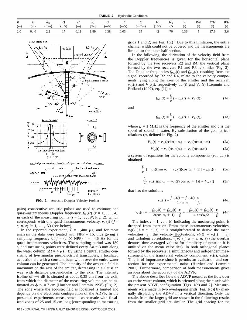
TABLE 2. Hydraulic Conditions

R(m)

B(m)

d50

(mm)Q

(L/s)H

(m)Ss

[‰]U

(m/s)u*

(m/s)C

(m1/2/s)R

(103)R*(/)

F(/)

R/B(/)

R/H(/)

B/H(/)

2.0 0.40 2.1 17 0.11 1.89 0.38 0.034 35 42 70 0.36 5 17.9 3.6

FIG. 2. Acoustic Doppler Velocity Profiler

pairs) consecutive acoustic pulses are used to estimate onequasi-instantaneous Doppler frequency, (r = 1, . . . , 4),f (t)Dr,i

in each of the measuring points (i = 1, . . . , N, Fig. 2), whichcorresponds with one quasi-instantaneous velocity, vj,i(t) ( j =s, n, z; i= 1, . . . , N) (see below).

In the reported experiment, T = 1,400 ms, and for mostanalysis the data were treated with NPP = 16, thus giving asampling frequency of f = (T 3 NPP)21 = 44.6 Hz for thequasi-instantaneous velocities. The sampling period was 180s, and measuring points were defined every Dn = 3 mm alongthe water column (Dt = 4 ms). By using a central emitter con-sisting of five annular piezoelectrical transducers, a focalizedacoustic field with a constant beamwidth over the entire watercolumn can be generated. The intensity of the acoustic field ismaximum on the axis of the emitter, decreasing in a Gaussianway with distance perpendicular to the axis. The intensityisoline of 26 dB is situated at about 0.35 cm from the axis,from which the diameter of the measuring volume can be es-timated as f ' 0.7 cm (Hurther and Lemmin 1998) (Fig. 2).The zone where the acoustic field is focalized is limited anddepends on the electronic configuration of the ADVP. In thepresented experiments, measurements were made with focal-ized zones of 25 and 15 cm long [corresponding to measuring


grids 1 and 2; see Fig. 1(c)]. Due to this limitation, the entirechannel width could not be covered and the measurements arelimited to the outer half-section.

In the following, the derivation of the velocity field fromthe Doppler frequencies is given for the horizontal planeformed by the two receivers R2 and R4; the vertical planeformed by the two receivers R1 and R3 is similar (Fig. 2).The Doppler frequencies and resulting from thef (t) f (t),D2,i D4,i

signal recorded by R2 and R4, relate to the velocity compo-nents lying along the axes of the emitter and the receiver,

and respectively and [Lemmin andv (t) V (t), v (t) V (t)n,i 2,i n,i 4,i

Rolland (1997), eq. (1)] as

fef (t) = (2v (t) 1 V (t)) (1a)D2, i n,i 2,i

c

and

fef (t) = (2v (t) 1 V (t)) (1b)D4, i n,i 4,i

c

where fe = 1 MHz is the frequency of the emitter and c is thespeed of sound in water. By substitution of the geometricalrelations (ai defined in Fig. 2)

V (t) = v (t)sin(2a ) 2 v (t)cos(2a ) (2a)2,i s,i i n,i i

V (t) = v (t)sin(a ) 2 v (t)cos(a ) (2b)4,i s,i i n,i i

a system of equations for the velocity components (vs,i, vn,i) isobtained

fe? [2v (t)sin a 2 v (t)(cos a 1 1)] = f (t) (3a)s,i i n, i i D2, i

c

fe? [v (t)sin a 2 v (t)(cos a 1 1)] = f (t) (3b)s,i i n,i i D4,i

c

that has the solutions

f (t) 2 f (t) cD4, i D2,iv (t) = ? (4a)s,i 2 sin a fi e

f (t) 1 f (t) c f (t) 1 f (t) cD4,i D2, i D4,i D2, iv (t) = 2 ? = 2 ? (4b)n,i 22(cos a 1 1) f 4 cos a /2 fi e i e

The index i = 1, . . . , N, indicating the measuring point, isdropped from there on. From these instantaneous velocities,vj(t) ( j = s, n, z), it is straightforward to derive the meanvelocities, vj, the velocity fluctuations, = vj (t) 2 vj,v9(t)j

and turbulent correlations, ( j, k = s, n, z) (the overbarv9v9j k

denotes time-averaged values; for simplicity of notation it isomitted on the mean velocities). In both orthogonal planesformed by the receivers, a simultaneous and independent mea-surement of the transversal velocity component, vn(t), exists.This is of importance since it permits an evaluation and cor-rection for the experimental noise (Hurther and Lemmin2001). Furthermore, comparison of both measurements givesan idea about the accuracy of the ADVP.

The above describes how the ADVP measures the flow overan entire water column, which is oriented along the n-axis withthe present ADVP configuration [Figs. 1(c) and 2]. Measure-ments were made in two overlapping grids [Fig. 1(c)] by man-ually displacing the ADVP in a vertical direction. Only theresults from the larger grid are shown in the following; resultsfrom the smaller grid are similar. The grid spacing for the

larger grid was 0.5 cm vertically (;H/22) and 0.3 cm trans-versally (;B/133), resulting in 1,360 measuring points. Theregions near the water surface and the bottom [indicated inFig. 1(c)] could not be measured with the adopted configura-tion of the ADVP (see below).

The ADVP sometimes produces results in a limited numberof measuring points that fall far outside the usual scatter. Thereare two reasons for these clearly erroneous measurements. (1)As explained in the section on the ADVP, the velocity in pointi (Fig. 2) on the transversal profile is derived from the back-scattered signal recorded at arrival time ti. It sometimes hap-pens that multiple-scattered parasitical echos reach the receiverat exactly the same arrival time, thus perturbating the mea-surement in point i. This effect is very local and only influ-ences a couple of points on the profiles. By carefully choosingthe ADVP configuration, this problem is strongly reduced andthese parasitical echos only occur occasionally. (2) In the re-ported experiment, the regions close to the water surface andto the bottom far away from the bank contained some clearlyerroneous points. This is while the flypath of the backscatteredsignal passes near the water surface or the bottom for pointsfar away from the bank. The influence of this surface andbottom proximity gave perturbations in some of the measuringpoints.

A goal of this research is to analyze experimentally the var-ious terms in the flow equations (momentum, vorticity, andenergy equations) and to derive the mixing coefficients. Thisrequires the evaluation of derivatives of the measured quan-

F(

tities (such as derivatives of mean velocities or turbulentstresses), which is difficult to do from the raw data becauseof the experimental scatter. Therefore, analytical surfaces havebeen fitted to the experimental data using 2D smoothingsplines with weight functions [de Boor (1978), chapters 14 and17]. Thanks to the weight functions, the measured data can beextended outside the measuring grid by imposing physicalboundary conditions (such as the no-slip condition on rigidboundaries and no shear parallel to the water surface). Thefitted surface is found as a compromise between smoothnessof the analytical surface [see de Boor (1978) for a mathematicaldescription] and proximity to the measured data, defined as

2w(n, z)(x (n, z) 2 x (n, z)) < tolerance (5)exp fitOgrid

in which w is the weight function, xexp are the experimentalvalues of the concerned variable, and xfit the approximation bysurface fitting to them. The choice of a compromise betweenboth criteria is subjective and has to be made separately foreach fitted quantity. Care has been taken not to introduce sys-tematic errors. This means that xexp 2 xfit should have a randomdistribution over the measuring grid with frequent signchanges along both the n- and z-directions. Thanks to the finemeasuring grid, this analytical surface fitting could be donewith a high precision.

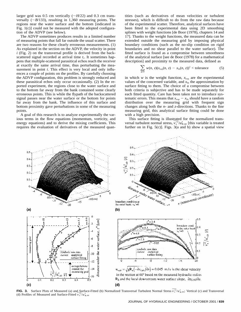
This surface fitting is illustrated for the normalized trans-versal turbulent normal stress, [this variable is treated2 2v9 /un ,60*further on in Fig. 5(c)]. Figs. 3(a and b) show a spatial view

IG. 3. Surface Plots of Measured (a) and Surface-Fitted (b) Normalized Transversal Turbulent Normal Stress Vertical (c) and Transversal2 2v 9 /u ;n ,60*d) Profiles of Measured and Surface-Fitted 2 2v 9 /un ,60*


of the raw data and the surface-fitted ones. Fig. 3(c) showsvertical profiles of the raw and the fitted data at some char-acteristic locations [close to the outer bank, in the outer-bankcell, at the separation between both cells, and in the center-region cell; see Fig. 4(b)]. Similarly, Fig. 3(d) shows sometransversal profiles distributed over the measuring grid. At theouter bank, the physical boundary condition, = 0, has been2v9nimposed [Figs. 3(b and d)]. The fitted surface closely followsthe raw data and conserves all its characteristic features, butsmooths the scatter. The analytically fitted surfaces are usedfor most analysis of the data and for their further presentationin this paper.

The accuracy of the measurements has been evaluated in-directly by

1. Comparing the results of the measurements made on thetwo overlapping grids with different configurations of theADVP

2. Comparing the two simultaneous and independent mea-surements of the transversal velocity component, vn(t)

3. Evaluating a coefficient of determination of the surfacefitting procedure, defined as [Lancaster and Salkauskas(1986), p. 55]

2(x 2 x )exp fitO2R = 1 2 (6)

2(x 2 ^^x &&)exp expOin which ^^xexp&& is the average value over the measuringgrid of xexp. The summation is done over the measuringgrid; clearly erroneous data (explained before) have been


omitted. This coefficient gives an idea about the scatteron the data. This scatter includes systematic errors dueto inaccuracy of the ADVP alignment as well as randomscatter inherent to experimental measurements.

An estimation of the accuracy and the coefficient of deter-mination of the surface-fitting procedure are reported in Figs.4–6. Overall, a high accuracy was obtained. The accuracy ofthe mean velocities was slightly better than that of the turbu-lent normal stresses, followed by the turbulent shear stresses.In general, the uncertainty increased somewhat with distancefrom the bank. Close to fixed boundaries (in the region ofabout 20% of the water depth), the measurements of the tur-bulent stresses are not very reliable, which is mainly due tothe large gradient in the mean velocity that exists in the mea-suring volumes. Care should be taken with the interpretationof boundary shear stresses, which can only be estimated afterbridging this region through extrapolation. The mean velocitymeasurements remain accurate close to the fixed boundaries.A detailed analysis of the precision and accuracy of measure-ments made with the ADVP is presented by Hurther andLemmin (2001).

EXPERIMENTAL RESULTS

Time-Averaged Velocities

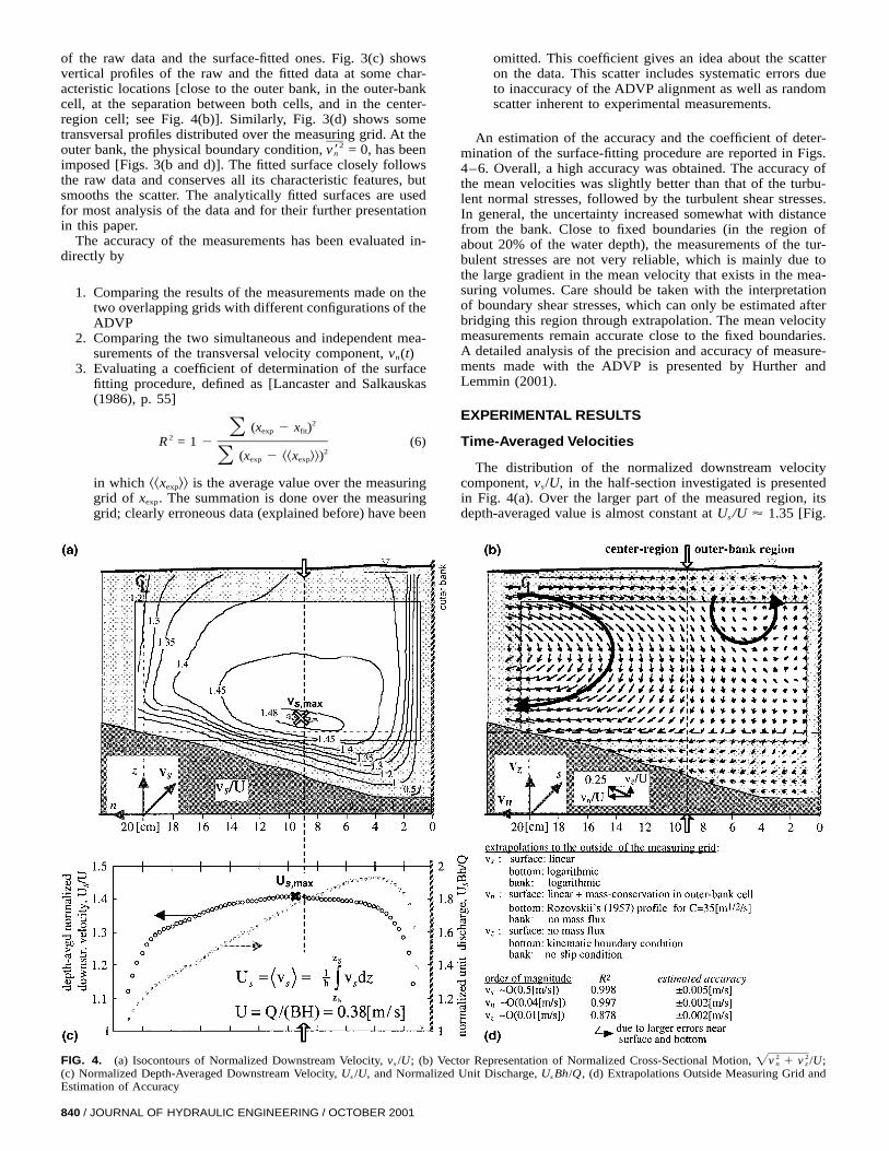
The distribution of the normalized downstream velocitycomponent, vs/U, in the half-section investigated is presentedin Fig. 4(a). Over the larger part of the measured region, itsdepth-averaged value is almost constant at Us/U ' 1.35 [Fig.

FIG. 4. (a) Isocontours of Normalized Downstream Velocity, vs /U; (b) Vector Representation of Normalized Cross-Sectional Motion, 2 2v 1 v /U;Ï n z

(c) Normalized Depth-Averaged Downstream Velocity, Us /U, and Normalized Unit Discharge, Us Bh/Q, (d) Extrapolations Outside Measuring Grid andEstimation of Accuracy

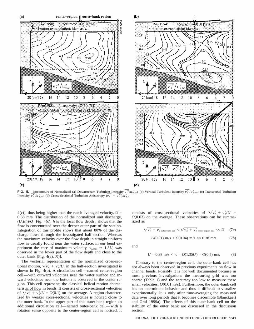
FIG. 5. Isocontours of Normalized (a) Downstream Turbulent Intensity (b) Vertical Turbulent Intensity (c) Transversal Turbulent2 2 2 2v 9 /u ; v 9 /u ;s ,60 z ,60* *Intensity (d) Cross-Sectional Turbulent Anisotropy (2 2 2 2 2v 9 /u ; v 9 2 v 9 )/un ,60 n z ,60* *

4(c)], thus being higher than the reach-averaged velocity, U =0.38 m/s. The distribution of the normalized unit discharge,(UsBh)/Q [Fig. 4(c); h is the local flow depth], shows that theflow is concentrated over the deeper outer part of the section.Integration of this profile shows that about 80% of the dis-charge flows through the investigated half-section. Whereasthe maximum velocity over the flow depth in straight uniformflow is usually found near the water surface, in our bend ex-periment the core of maximum velocity, vs,max ' 1.5U, wasobserved in the lower part of the flow depth and close to theouter bank [Fig. 4(a), X)].

The vectorial representation of the normalized cross-sec-tional motion, in the half-section investigated is2 2v 1 v /U,Ï n z

shown in Fig. 4(b). A circulation cell—named center-regioncell—with outward velocities near the water surface and in-ward velocities near the bottom is observed in the center re-gion. This cell represents the classical helical motion charac-teristic of flow in bends. It consists of cross-sectional velocitiesof = O(0.1) on the average. A region character-2 2v 1 v /UÏ n z

ized by weaker cross-sectional velocities is noticed close tothe outer bank. In the upper part of this outer-bank region anadditional circulation cell—named outer-bank cell—with arotation sense opposite to the center-region cell is noticed. It

consists of cross-sectional velocities of =2 2v 1 v /UÏ n z

O(0.03) on the average. These observations can be summa-rized as

2 2 2 2v 1 v < v 1 v << U (7a)Ï Ïn z outer-bank cell n z center-region cell

O(0.01) m/s < O(0.04) m/s << 0.38 m/s (7b)

and

U = 0.38 m/s < v = O(1.35U ) = O(0.5) m/s (8)s

Contrary to the center-region cell, the outer-bank cell hasnot always been observed in previous experiments on flow inchannel bends. Possibly it is not well documented because inmost previous investigations the measuring grid was toocoarse (Table 1) and the accuracy too low to measure thesesmall velocities, O(0.01 m/s). Furthermore, the outer-bank cellhas an intermittent behavior and thus is difficult to visualizeexperimentally. It is only after time-averaging the measureddata over long periods that it becomes discernible (Blanckaertand Graf 1999a). The effects of this outer-bank cell on thestability of the outer bank are discussed in the discussionsection.


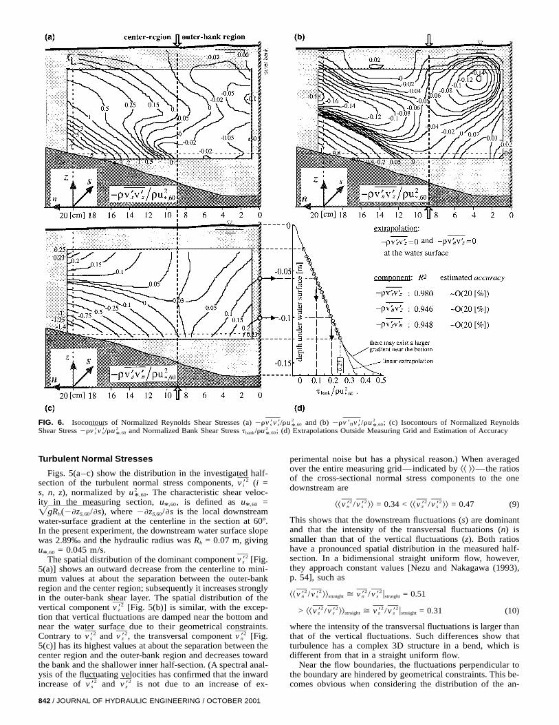
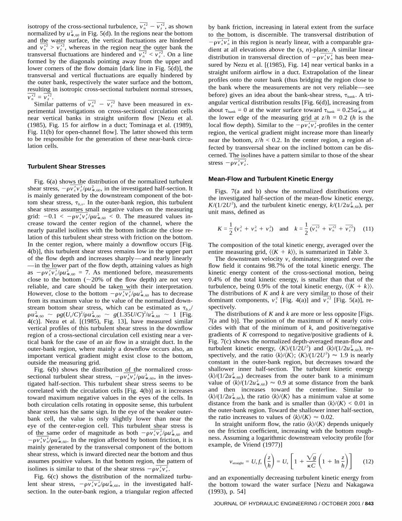
FIG. 6. Isocontours of Normalized Reynolds Shear Stresses (a) and (b) (c) Isocontours of Normalized Reynolds2 22rv 9v 9/ru 2rv 9 v 9/ru ;ns z ,60 z ,60* *Shear Stress and Normalized Bank Shear Stress (d) Extrapolations Outside Measuring Grid and Estimation of Accuracy2 22rv 9v 9/ru t /ru ;s n ,60 bank ,60* *

Turbulent Normal Stresses

Figs. 5(a–c) show the distribution in the investigated half-section of the turbulent normal stress components, (i =2v 9is, n, z), normalized by The characteristic shear veloc-2u .,60*ity in the measuring section, u*,60, is defined as u*,60 =

where 2zS,60/s is the local downstreamgR (2z /s),Ï h S,60

water-surface gradient at the centerline in the section at 607.In the present experiment, the downstream water surface slopewas 2.89‰ and the hydraulic radius was Rh = 0.07 m, givingu*,60 = 0.045 m/s.

The spatial distribution of the dominant component [Fig.2v 9s5(a)] shows an outward decrease from the centerline to mini-mum values at about the separation between the outer-bankregion and the center region; subsequently it increases stronglyin the outer-bank shear layer. The spatial distribution of thevertical component [Fig. 5(b)] is similar, with the excep-2v 9ztion that vertical fluctuations are damped near the bottom andnear the water surface due to their geometrical constraints.Contrary to and the transversal component [Fig.2 2 2v 9 v 9 , v9s z n

5(c)] has its highest values at about the separation between thecenter region and the outer-bank region and decreases towardthe bank and the shallower inner half-section. (A spectral anal-ysis of the fluctuating velocities has confirmed that the inwardincrease of and is not due to an increase of ex-2 2v 9 v9s z


perimental noise but has a physical reason.) When averagedover the entire measuring grid—indicated by ^^ &&—the ratiosof the cross-sectional normal stress components to the onedownstream are

2 2 2 2^^v 9 /v 9 && = 0.34 < ^^v 9 /v 9 && = 0.47 (9)n s z s

This shows that the downstream fluctuations (s) are dominantand that the intensity of the transversal fluctuations (n) issmaller than that of the vertical fluctuations (z). Both ratioshave a pronounced spatial distribution in the measured half-section. In a bidimensional straight uniform flow, however,they approach constant values [Nezu and Nakagawa (1993),p. 54], such as

2 2 2 2^^v 9 /v 9 && > v 9 /v 9 u = 0.51n s straight n s straight

2 2 2 2> ^^v 9 /v 9 && > v 9 /v 9 u = 0.31z s straight z s straight (10)

where the intensity of the transversal fluctuations is larger thanthat of the vertical fluctuations. Such differences show thatturbulence has a complex 3D structure in a bend, which isdifferent from that in a straight uniform flow.

Near the flow boundaries, the fluctuations perpendicular tothe boundary are hindered by geometrical constraints. This be-comes obvious when considering the distribution of the an-

isotropy of the cross-sectional turbulence, 2 as shown2 2v 9 v 9 ,n z

normalized by in Fig. 5(d). In the regions near the bottom2u ,60*and the water surface, the vertical fluctuations are hinderedand > whereas in the region near the outer bank the2 2v 9 v 9 ,n z

transversal fluctuations are hindered and < On a line2 2v 9 v9 .n z

formed by the diagonals pointing away from the upper andlower corners of the flow domain [dark line in Fig. 5(d)], thetransversal and vertical fluctuations are equally hindered bythe outer bank, respectively the water surface and the bottom,resulting in isotropic cross-sectional turbulent normal stresses,

=2 2v 9 v 9 .n z

Similar patterns of 2 have been measured in ex-2 2v 9 v 9n z

perimental investigations on cross-sectional circulation cellsnear vertical banks in straight uniform flow [Nezu et al.(1985), Fig. 15 for airflow in a duct; Tominaga et al. (1989),Fig. 11(b) for open-channel flow]. The latter showed this termto be responsible for the generation of these near-bank circu-lation cells.

Turbulent Shear Stresses

Fig. 6(a) shows the distribution of the normalized turbulentshear stress, in the investigated half-section. It22rv 9v 9/ru ,s z ,60*is mainly generated by the downstream component of the bot-tom shear stress, tb,s. In the outer-bank region, this turbulentshear stress assumes small negative values on the measuringgrid: 20.1 < < 0. The measured values in-22rv 9v9/rus z ,60*crease toward the center region of the channel, where thenearly parallel isolines with the bottom indicate the close re-lation of this turbulent shear stress with friction on the bottom.In the center region, where mainly a downflow occurs [Fig.4(b)], this turbulent shear stress remains low in the upper partof the flow depth and increases sharply—and nearly linearly—in the lower part of the flow depth, attaining values as highas = 7. As mentioned before, measurements22rv 9v 9/rus z ,60*close to the bottom (;20% of the flow depth) are not veryreliable, and care should be taken with their interpretation.However, close to the bottom has to decrease22rv9v 9/rus z ,60*from its maximum value to the value of the normalized down-stream bottom shear stress, which can be estimated as tb,s/

; rg(Us/C)2/ ; g(1.35U/C)2/ ; 1 [Fig.2 2 2ru ru u,60 ,60 ,60* * *4(c)]. Nezu et al. [(1985), Fig. 13], have measured similarvertical profiles of this turbulent shear stress in the downflowregion of a cross-sectional circulation cell existing near a ver-tical bank for the case of an air flow in a straight duct. In theouter-bank region, where mainly a downflow occurs also, animportant vertical gradient might exist close to the bottom,outside the measuring grid.

Fig. 6(b) shows the distribution of the normalized cross-sectional turbulent shear stress, in the inves-22rv 9v 9/ru ,n z ,60*tigated half-section. This turbulent shear stress seems to becorrelated with the circulation cells [Fig. 4(b)] as it increasestoward maximum negative values in the eyes of the cells. Inboth circulation cells rotating in opposite sense, this turbulentshear stress has the same sign. In the eye of the weaker outer-bank cell, the value is only slightly lower than near theeye of the center-region cell. This turbulent shear stress isof the same order of magnitude as both and22rv 9v 9/rus z ,60*

In the region affected by bottom friction, it is22rv 9v 9/ru .s n ,60*mainly generated by the transversal component of the bottomshear stress, which is inward directed near the bottom and thusassumes positive values. In that bottom region, the pattern ofisolines is similar to that of the shear stress 2rv9v 9.s z

Fig. 6(c) shows the distribution of the normalized turbu-lent shear stress, in the investigated half-22rv 9v 9/ru ,s n ,60*section. In the outer-bank region, a triangular region affected

by bank friction, increasing in lateral extent from the surfaceto the bottom, is discernible. The transversal distribution of

in this region is nearly linear, with a comparable gra-2rv 9v 9s n

dient at all elevations above the (s, n)-plane. A similar lineardistribution in transversal direction of has been mea-2rv 9v 9s n

sured by Nezu et al. [(1985), Fig. 14] near vertical banks in astraight uniform airflow in a duct. Extrapolation of the linearprofiles onto the outer bank (thus bridging the region close tothe bank where the measurements are not very reliable—seebefore) gives an idea about the bank-shear stress, tbank. A tri-angular vertical distribution results [Fig. 6(d)], increasing fromabout tbank = 0 at the water surface toward tbank = at20.25u ,60*the lower edge of the measuring grid at z/h = 0.2 (h is thelocal flow depth). Similar to the -profiles in the center2rv 9v9s z

region, the vertical gradient might increase more than linearlynear the bottom, z/h < 0.2. In the center region, a region af-fected by transversal shear on the inclined bottom can be dis-cerned. The isolines have a pattern similar to those of the shearstress 2rv 9v 9.s z

Mean-Flow and Turbulent Kinetic Energy

Figs. 7(a and b) show the normalized distributions overthe investigated half-section of the mean-flow kinetic energy,K/(1/2U 2), and the turbulent kinetic energy, per2k/(1/2u ),,60*unit mass, defined as

1 12 2 2 2 2 2K = (v 1 v 1 v ) and k = (v 9 1 v 9 1 v 9 ) (11)s n z s n z2 2

The composition of the total kinetic energy, averaged over theentire measuring grid, ^^K 1 k&&, is summarized in Table 3.

The downstream velocity vs dominates; integrated over theflow field it contains 98.7% of the total kinetic energy. Thekinetic energy content of the cross-sectional motion, being0.4% of the total kinetic energy, is smaller than that of theturbulence, being 0.9% of the total kinetic energy, ^^K 1 k &&.The distributions of K and k are very similar to those of theirdominant components, [Fig. 4(a)] and [Fig. 5(a)], re-2 2v v 9s s

spectively.The distributions of K and k are more or less opposite [Figs.

7(a and b)]. The position of the maximum of K nearly coin-cides with that of the minimum of k, and positive/negativegradients of K correspond to negative/positive gradients of k.Fig. 7(c) shows the normalized depth-averaged mean-flow andturbulent kinetic energy, ^K&/(1/2U 2) and re-2^k&/(1/2u ),,60*spectively, and the ratio ^k&/^K&; ^K&/(1/2U 2) ' 1.9 is nearlyconstant in the outer-bank region, but decreases toward theshallower inner half-section. The turbulent kinetic energy

decreases from the outer bank to a minimum2^k&/(1/2u ),60*value of ' 0.9 at some distance from the bank2^k&/(1/2u ),60*and then increases toward the centerline. Similar to

the ratio ^k&/^K& has a minimum value at some2^k&/(1/2u ),,60*distance from the bank and is smaller than ^k&/^K& < 0.01 inthe outer-bank region. Toward the shallower inner half-section,the ratio increases to values of ^k&/^K& ' 0.02.

In straight uniform flow, the ratio ^k&/^K& depends uniquelyon the friction coefficient, increasing with the bottom rough-ness. Assuming a logarithmic downstream velocity profile [forexample, de Vriend (1977)]

z g zÏv = U f = U 1 1 1 1 ln (12)straight s s sS D F S DGh kC h

and an exponentially decreasing turbulent kinetic energy fromthe bottom toward the water surface [Nezu and Nakagawa(1993), p. 54]


FIG. 7. Isocontours of Normalized (a) Mean Flow Kinetic Energy K/(1/2U 2); (b) Turbulent Kinetic Energy (c) Depth-Averaged Nor-2k/(1/2u );,60*malized Mean Flow and Turbulent Kinetic Energy, ^K&/(1/2U 2) and and Ratio ^k&/^K&; (d) Vertical Profiles of in Straight Flow2 2^k&/(1/2u ), k/(1/2u ),60 ,60* *and Bend Flow (Measured)

TABLE 3. Composition of Total Kinetic Energy, Averaged overEntire Measuring Grid

(1024 m2/s2) (1024 m2/s2)

= 1,316.5 [Fig. 4(a)]1 2^^v &&s2

= 6.75 [Fig. 5(a)]1 2^^v9 &&s2

= 4.69 [Fig. 4(b)]1 2^^v &&n2

= 2.3 [Fig. 5(b)]1 2^^v9 &&n2

= 0.86 [Fig. 4(b)]1 2^^v &&z2

= 3.15 [Fig. 5(c)]1 2^^v9 &&z2

^^K&& = 1,322 [Fig. 7(a)] ^^k&& = 12.2 [Fig. 7(b)]

2 22(z/h)k = 4.78u e (13)straight *

it is found by integration of (12) and (13) over the flow depththat

2^k& ^k & 4.133 u 4.133 g gstraight *= = ? = ? ' 4.1U S D2 2 2 2^K& 1 ^ f & U ^ f & C Cs s sstraight 2^v &straight2

(14)

For the earlier estimated bottom roughness, C ' 35 m1/2/s, aratio of ^k&/^K& ' 0.03 would be expected, which is nearly thecase toward the inner half-section but is higher than the ob-served value, ^k&/^K& < 0.01, in the outer-bank region.


In Fig. 7(d), the vertical profile of as found2k /(1/2u )straight ,60*in straight uniform flow—according to (13) and based on u*= U=g/C with C ' 35 m1/2/s—is compared with the verticalprofiles of measured at 5.9 and 17.9 cm from the2k/(1/2u ),60*outer bank. Whereas the straight flow profile decreases expo-nentially from the bottom toward the water surface, the mea-sured profiles decrease from the bottom to a minimum valueand then increase toward a maximum value near the watersurface [see also Fig. 7(b)]. Muto [(1997), Figs. 4.10, 23, 36,49, 57] and Tamai and Ikeya [(1985), Fig. 3(d)] have measuredsimilar profiles in a meandering channel.

DISCUSSION

The most important features observed in our experiment arethe existence of an outer-bank cell of secondary circulation[Fig. 4(b)] and the reduced level of turbulent activity in theregion near the outer bank [Fig. 7(c)]. Their influence on thestability of the outer bank and the adjacent bottom will bediscussed.

As already mentioned in the introduction, bankline stabili-zation is a major task in river management. Some recent pa-pers witness the increased interest in the erosional behavior ofthe channel banks and their modeling. Thorne (1982) has rec-ognized two dominant processes of bank erosion and retreat:basal erosion and geotechnical bank failure. Basal erosionsteepens the bank and intermittently causes mass bank failure.Duan et al. (1999) presented a detailed model of bank retreatthrough basal erosion, driven by the bank shear stress. A

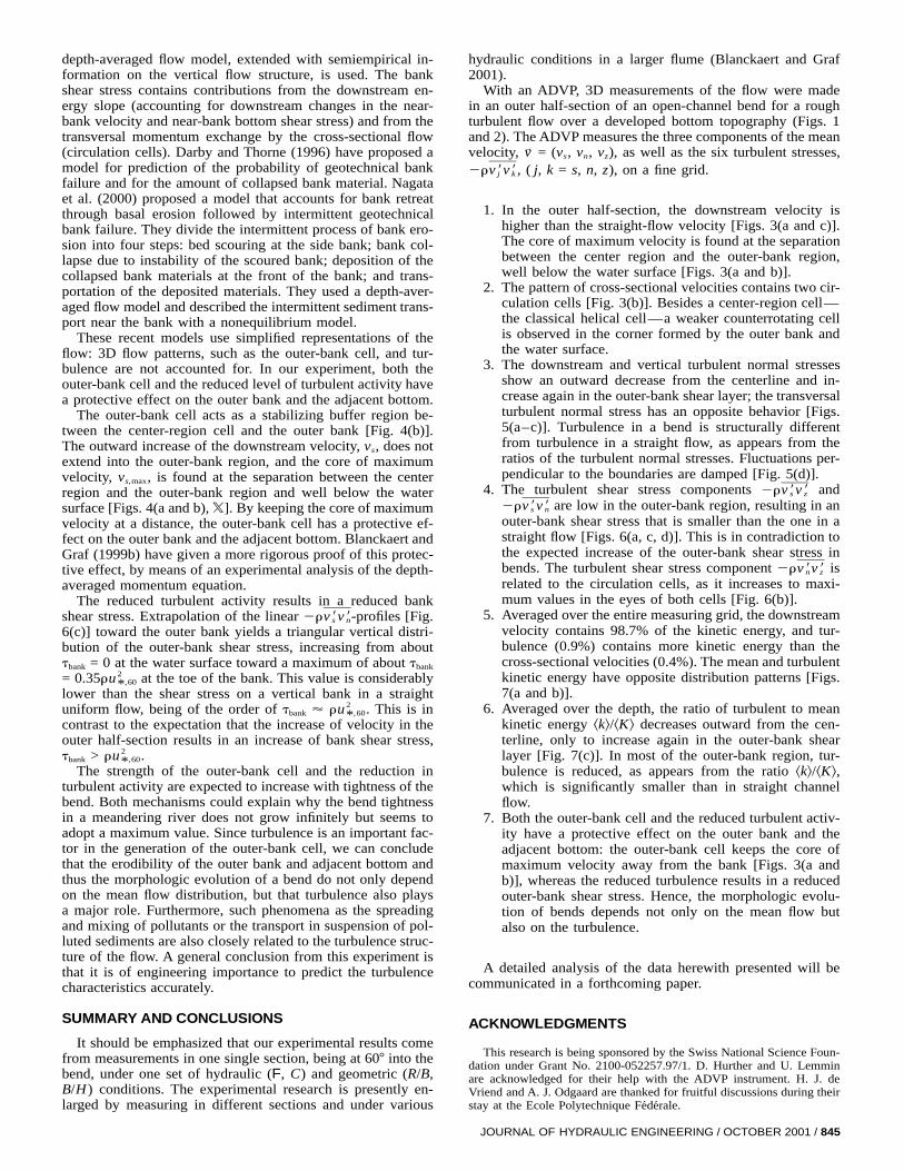
depth-averaged flow model, extended with semiempirical in-formation on the vertical flow structure, is used. The bankshear stress contains contributions from the downstream en-ergy slope (accounting for downstream changes in the near-bank velocity and near-bank bottom shear stress) and from thetransversal momentum exchange by the cross-sectional flow(circulation cells). Darby and Thorne (1996) have proposed amodel for prediction of the probability of geotechnical bankfailure and for the amount of collapsed bank material. Nagataet al. (2000) proposed a model that accounts for bank retreatthrough basal erosion followed by intermittent geotechnicalbank failure. They divide the intermittent process of bank ero-sion into four steps: bed scouring at the side bank; bank col-lapse due to instability of the scoured bank; deposition of thecollapsed bank materials at the front of the bank; and trans-portation of the deposited materials. They used a depth-aver-aged flow model and described the intermittent sediment trans-port near the bank with a nonequilibrium model.

These recent models use simplified representations of theflow: 3D flow patterns, such as the outer-bank cell, and tur-bulence are not accounted for. In our experiment, both theouter-bank cell and the reduced level of turbulent activity havea protective effect on the outer bank and the adjacent bottom.

The outer-bank cell acts as a stabilizing buffer region be-tween the center-region cell and the outer bank [Fig. 4(b)].The outward increase of the downstream velocity, vs, does notextend into the outer-bank region, and the core of maximumvelocity, vs,max, is found at the separation between the centerregion and the outer-bank region and well below the watersurface [Figs. 4(a and b), X]. By keeping the core of maximumvelocity at a distance, the outer-bank cell has a protective ef-fect on the outer bank and the adjacent bottom. Blanckaert andGraf (1999b) have given a more rigorous proof of this protec-tive effect, by means of an experimental analysis of the depth-averaged momentum equation.

The reduced turbulent activity results in a reduced bankshear stress. Extrapolation of the linear -profiles [Fig.2rv 9v9s n

6(c)] toward the outer bank yields a triangular vertical distri-bution of the outer-bank shear stress, increasing from abouttbank = 0 at the water surface toward a maximum of about tbank

= at the toe of the bank. This value is considerably20.35ru ,60*lower than the shear stress on a vertical bank in a straightuniform flow, being of the order of tbank ' This is in2ru .,60*contrast to the expectation that the increase of velocity in theouter half-section results in an increase of bank shear stress,tbank > 2ru .,60*

The strength of the outer-bank cell and the reduction inturbulent activity are expected to increase with tightness of thebend. Both mechanisms could explain why the bend tightnessin a meandering river does not grow infinitely but seems toadopt a maximum value. Since turbulence is an important fac-tor in the generation of the outer-bank cell, we can concludethat the erodibility of the outer bank and adjacent bottom andthus the morphologic evolution of a bend do not only dependon the mean flow distribution, but that turbulence also playsa major role. Furthermore, such phenomena as the spreadingand mixing of pollutants or the transport in suspension of pol-luted sediments are also closely related to the turbulence struc-ture of the flow. A general conclusion from this experiment isthat it is of engineering importance to predict the turbulencecharacteristics accurately.

SUMMARY AND CONCLUSIONS

It should be emphasized that our experimental results comefrom measurements in one single section, being at 607 into thebend, under one set of hydraulic (F, C) and geometric (R/B,B/H ) conditions. The experimental research is presently en-larged by measuring in different sections and under various

hydraulic conditions in a larger flume (Blanckaert and Graf2001).

With an ADVP, 3D measurements of the flow were madein an outer half-section of an open-channel bend for a roughturbulent flow over a developed bottom topography (Figs. 1and 2). The ADVP measures the three components of the meanvelocity, = (vs, vn, vz), as well as the six turbulent stresses,→v

( j, k = s, n, z), on a fine grid.2rv 9v 9,j k

1. In the outer half-section, the downstream velocity ishigher than the straight-flow velocity [Figs. 3(a and c)].The core of maximum velocity is found at the separationbetween the center region and the outer-bank region,well below the water surface [Figs. 3(a and b)].

2. The pattern of cross-sectional velocities contains two cir-culation cells [Fig. 3(b)]. Besides a center-region cell—the classical helical cell—a weaker counterrotating cellis observed in the corner formed by the outer bank andthe water surface.

3. The downstream and vertical turbulent normal stressesshow an outward decrease from the centerline and in-crease again in the outer-bank shear layer; the transversalturbulent normal stress has an opposite behavior [Figs.5(a–c)]. Turbulence in a bend is structurally differentfrom turbulence in a straight flow, as appears from theratios of the turbulent normal stresses. Fluctuations per-pendicular to the boundaries are damped [Fig. 5(d)].

4. The turbulent shear stress components and2rv 9v 9s z

are low in the outer-bank region, resulting in an2rv 9v 9s n

outer-bank shear stress that is smaller than the one in astraight flow [Figs. 6(a, c, d)]. This is in contradiction tothe expected increase of the outer-bank shear stress inbends. The turbulent shear stress component is2rv 9v 9n z

related to the circulation cells, as it increases to maxi-mum values in the eyes of both cells [Fig. 6(b)].

5. Averaged over the entire measuring grid, the downstreamvelocity contains 98.7% of the kinetic energy, and tur-bulence (0.9%) contains more kinetic energy than thecross-sectional velocities (0.4%). The mean and turbulentkinetic energy have opposite distribution patterns [Figs.7(a and b)].

6. Averaged over the depth, the ratio of turbulent to meankinetic energy ^k&/^K& decreases outward from the cen-terline, only to increase again in the outer-bank shearlayer [Fig. 7(c)]. In most of the outer-bank region, tur-bulence is reduced, as appears from the ratio ^k&/^K&,which is significantly smaller than in straight channelflow.

7. Both the outer-bank cell and the reduced turbulent activ-ity have a protective effect on the outer bank and theadjacent bottom: the outer-bank cell keeps the core ofmaximum velocity away from the bank [Figs. 3(a andb)], whereas the reduced turbulence results in a reducedouter-bank shear stress. Hence, the morphologic evolu-tion of bends depends not only on the mean flow butalso on the turbulence.

A detailed analysis of the data herewith presented will becommunicated in a forthcoming paper.

ACKNOWLEDGMENTS

This research is being sponsored by the Swiss National Science Foun-dation under Grant No. 2100-052257.97/1. D. Hurther and U. Lemminare acknowledged for their help with the ADVP instrument. H. J. deVriend and A. J. Odgaard are thanked for fruitful discussions during theirstay at the Ecole Polytechnique Federale.


REFERENCES

Anwar, H. O. (1986). ‘‘Turbulent structure in a river bed.’’ J. Hydr.Engrg., ASCE, 112(8), 657–669.

Blanckaert, K., and Graf, W. H. (1999a). ‘‘Experiments on flow in open-channel bends.’’ Proc., 28th Congr. Int. Assoc. Hydr. Res., TechnicalUniversity of Graz, Austria (CD-ROM).

Blanckaert, K., and Graf, W. H. (1999b). ‘‘Outer-bank cell of secondarycirculation and boundary shear stress in open-channel bends.’’ Proc.,Symp. on River, Coastal and Estuarine Morphodynamics, University ofGenova, Italy, Vol. 1, 533–543.

Blanckaert, K., and Graf, W. H. (2001). ‘‘Experiments on flow in astrongly curved channel bend.’’ Proc., 29th Congr. Int. Assoc. Hydr.Res. and Engrg., Chinese Hydraulic Engineering Society, Beijing,China (in press).

Darby, S. E., and Thorne, C. R. (1996). ‘‘Development and testing ofriverbank-stability analysis.’’ J. Hydr. Engrg., ASCE, 122(8), 443–454.

de Boor, C. (1978). A practical guide to splines, Springer, New York.de Vriend, H. J. (1977). ‘‘A mathematical model of steady flow in curved

shallow channels.’’ J. Hydr. Res., Delft, The Netherlands, 15(1), 37–54.

de Vriend, H. J. (1979). ‘‘Flow measurements in a curved rectangularchannel.’’ Rep. No. 9-79, Lab. Fluid Mech., Dept. of Civ. Engrg., DelftUniversity of Technology, The Netherlands.

de Vriend, H. J. (1981). ‘‘Flow measurements in a curved rectangularchannel. II: Rough bottom.’’ Rep. No. 5-81, Lab. Fluid Mech., Dept.of Civ. Engrg., Delft University of Technology, The Netherlands.

de Vriend, H. J., and Struiksma, N. (1984). ‘‘Flow and bed deformationin river bends.’’ River meandering, C. M. Elliot, ed., ASCE, New York,810–828.

Dietrich, W. E. (1987). ‘‘Mechanics of flow and sediment transport inriver bends.’’ River channels: Environment and process. K. Richards,ed., Institute of British Geography, Oxford, U.K.

Dietrich, W. E., and Smith, J. D. (1983). ‘‘Influence of the point bar onflow through curved channels.’’ Water Resour. Res., 19(5), 1173–1192.

Duan, G., Jia, Y., and Wang, S. (1999). ‘‘Simulation of meandering chan-nel migration processes with the enhanced CCHE2D.’’ Proc., 28thCongr. Int. Assoc. Hydr. Res., Technical University of Graz, Austria(CD-ROM).

Gotz, W. (1975). ‘‘Sekundarstromungen in aufeinander folgenden Ger-innekrummungen.’’ Rep. No. 163, Theodor-Rehbock Flussbaulabora-torium, Karlsruhe, Germany.

Hurther, D., and Lemmin, U. (1998). ‘‘A constant beamwidth transducerfor three-dimensional Doppler profile measurements in open channelflow.’’ Measurement Science and Technology, 9(10), 1706–1714.

Hurther, D., and Lemmin, U. (2001). ‘‘A correction method for turbulencemeasurements with a 3-D acoustic Doppler velocity profiler.’’ J. Atm.Oc. Techn, Vol. 18, 446–458.

Lancaster, P., and Salkauskas, K. (1986). Curve and surface fitting: Anintroduction, Academic Press, London.

Lemmin, U., and Rolland, T. (1997). ‘‘Acoustic velocity profiler for lab-oratory and field studies.’’ J. Hydr. Engrg., ASCE, 123(12), 1089–1098.

Muto, Y. (1997). ‘‘Turbulent flow in two-stage meandering channels.’’PhD thesis, University of Bradford, U.K.

Nagata, N., Hosoda, T., and Muramoto, Y. (2000). ‘‘Numerical analysisof river channel processes with bank erosion.’’ J. Hydr. Engrg., ASCE,126(4), 243–252.

Nezu, I., and Nakagawa, H. (1993). Turbulence in open-channel flows,Balkema, Rotterdam, The Netherlands.

Nezu, I., Nakagawa, H., and Tominaga, A. (1985). ‘‘Secondary currentsin a straight channel flow and the relation to its aspect ratio.’’ Turbulentshear flows 4, L. J. S. Bradbury et al., eds., Springer, Berlin, 246–260.

Odgaard, A. J. (1984). ‘‘Bank erosion contribution to stream sedimentload.’’ IIHR Rep. No. 280, Iowa Institute of Hydraulic Research, IowaCity.

Odgaard, A. J. (1986). ‘‘Meander flow model. I: Development.’’ J. Hydr.Engrg., ASCE, 112(12), 1117–1136.

Odgaard, A. J., and Bergs, M. A. (1988). ‘‘Flow processes in a curvedalluvial channel.’’ Water Resour. Res., 24(1), 45–56.

Parker, G., and Johannesson, H. (1989). ‘‘Observations on several recenttheories of resonance and overdeepening in meandering channels.’’River meandering, S. Ikeda and G. Parker, eds., Water Resour. Mono-graph 12, American Geophysical Union, Washington, D.C., 379–415.

Rozovskii, I. L. (1957). Flow of water in bends of open channels, Acad-emy of Sciences of the Ukrainian SSR, Kiev, 1957; Israel Program forScientific Translations, Jerusalem, 1961.

Shiono, K., and Muto, Y. (1998). ‘‘Complex flow mechanisms in com-pound meandering channels with overbank flow.’’ J. Fluid Mech., Vol.376, 221–261.

Siebert, W. (1982). ‘‘Stromungscharakteristiken in einem Kanal mit 1807-


Krummungen.’’ Rep. No. 168, Theodor-Rehbock Flussbaulaboratorium,Karlsruhe, Germany.

Steffler, P. M. (1984). ‘‘Turbulent flow in a curved rectangular channel.’’PhD thesis, University of Alberta, Canada.

Strickler, A. (1923). ‘‘Beitrage zur Frage der Geschwindigkeitsformeln.’’Rep. No. 16, Amt. f. Wasserwirtschaft, Bern, Switzerland.

Tamai, N., and Ikeya, T. (1985). ‘‘Three-dimensional flow over alternatingpoint bars in a meandering channel.’’ J. Hydrosci. Hydr. Engrg., 3(1),1–13.

Thorne, C. R. (1982). ‘‘Processes and mechanisms of river bank erosion.’’Gravel-bed rivers, R. D. Hey, J. C. Bathurst, et al., eds., Wiley, NewYork, 227–259.

Tominaga, A., Ezaki, K., Nezu, I., and Nakagawa, H. (1989). ‘‘Three-dimensional turbulent structure in straight channel flows.’’ J. Hydr.Res., Delft, The Netherlands, 27(1), 149–173.

Tominaga, A., Nagao, M., and Nezu, I. (1999). ‘‘Flow structure and mo-mentum transport processes in curved open-channels with vegetation.’’Proc., 28th Congr. Int. Assoc. Hydr. Res., Technical University of Graz,Austria (CD-ROM).

NOTATION

The following symbols are used in this paper:

ADVP = acoustic Doppler velocity profiler;B = channel width;C = Chezy roughness coefficient;c = celerity of sound in water, c = 1,500 m/s at 207;

d50 = mean diameter of sand bottom;F = Froude number = ;U/ gHÏfs = normalized vertical profiles of downstream ve-

locity component, vs;fDr = Doppler signal recorded by receiver r, r = 1, 2,

3, 4;fe = frequency of emitter, = 1 MHz;g = gravitational acceleration;H = reach-averaged flow depth;h = local flow depth;K = mean flow kinetic energy per unit mass;k = turbulent kinetic energy per unit mass;ks = Nikuradse equivalent sand roughness;N = number of measuring points on profile;

NPP = number of pair-pulses;n = transversal reference axis;

n* = distance from outer bank;prf = pulse repetition frequency;Q = discharge;R = radius of curvature of channel centerline;

R 2 = coefficient of determination of surface fitting;Rh = hydraulic radius of cross section;Rr = Receiver r, r = 1, 2, 3, 4;

R = UH/n = Reynolds number;R* = u*ks /n = particle Reynolds number;

Ss = reach-averaged water surface gradient on cen-terline;

s = downstream reference axis;t = time;

U = Q/(BH) = reach-averaged velocity;Us = depth-averaged downstream velocity;

u* = U=g/C = friction velocity;Vr = velocity component along axis of receiver r, r =

1, 2, 3, 4;vj = time-averaged velocity component, j = s, n, z;

vj (t) = instantaneous velocity component, j = s, n, z;v 9 (t)j = instantaneous velocity fluctuation, j = s, n, z;v 9v 9j k = time-averaged correlation of velocity fluctua-

tions, j, k = s, n, z;xexp = experimental data;xfit = approximation by surface fitting to xexp;

z = vertical reference axis; elevation above horizon-tal (s, n)-plane;

z* = distance under water surface;ai = angle defined in Fig. 2;

Dn = height of measuring volumes;

k = von Karman constant;n = molecular viscosity of water; n = 1.004 3 1026

m2/s at 207;r = density of water; r = 998.2 kg/m3 at 207;t = shear stress at flow boundary (bottom or bank);f = diameter of measuring volumes;

overbar = time-averaged values;^?& = values averaged over local flow depth;

^^?&& = values averaged over the measuring grid; andO(?) = order of magnitude of.

Subscripts

b = bottom;bank = values at outer bank;max = maximum magnitude over measuring grid of

variable;S = water surface;

straight = corresponding value in straight uniform flow;and

60 = value in the section at 607.


MEAN FLOW AND TURBULENCE IN OPEN-CHANNEL BEND …€¦ · · 2011-01-01JOURNAL OF HYDRAULIC...

Documents

Transcript of MEAN FLOW AND TURBULENCE IN OPEN-CHANNEL BEND …€¦ · · 2011-01-01JOURNAL OF HYDRAULIC...