MEAN CONVERGENCE OF LAGRANGE INTERPOLATION. Ill · transactions of the american mathhmatic ai....
30
TRANSACTIONS of the AMERICAN MATHHMATIC AI. SOCIETY Volume 2X2. Number 2. April I9K4 MEAN CONVERGENCEOF LAGRANGEINTERPOLATION. Ill BY PAULNEVAI1 Abstract. Necessary and sufficient conditions are found for weighted mean conver- gence of Lagrange and quasi-Lagrange interpolation based at the zeros of gener- alized Jacobi polynomials. 1. Introduction. Although the problem of finding necessary and sufficient condi- tions for weighted mean convergence of Lagrange interpolation based at the zeros of orthogonal polynomials was formulated over forty years ago by P. Erdös and P. Turan, nevertheless no significant progress was achieved until 1970 when R. Askey [1 and 2] partially solved the case of interpolating at zeros of Jacobi polynomials. Askey's approach was based on an idea dating back to J. Marcinkiewicz which consists of reducing the problem of mean convergence of Lagrange interpolation to that of orthogonal Fourier series. In order to accomplish this task certain quadrature sums had to be estimated in terms of integrals. This was successfully carried out by Askey for certain Jacobi weights. By proposing another approach to estimating quadrature sums and by refining Askey's techniques, I managed to improve Askey's results in [14] where I found sufficient conditions for weighted Lp (0 <p < oo) convergence of Lagrange interpolation based at the zeros of slightly generalized Jacobi polynomials. By solving Turán's problem in [13, p. 180] I showed that for 0 < p < oo the conditions given in [14] are necessary as well. The only limitation of the Fourier series method is that it requires the knowledge of convergence of Fourier series in the same weighted Lp space where the convergence of Lagrange interpola- tion is considered. Since at the present time nothing is known about convergence of orthogonal Fourier series in Lp spaces with arbitrary weights, one is forced to look for other approaches when considering convergence of Lagrange interpolation in Lp spaces with general weights. It is demonstrated in this paper that by realizing that, in fact, Lagrange interpolation can be looked at as a mapping from bounded functions into the weighted Lp space rather than as a mapping from Lp into Lp, one can directly estimate Lp norms without referring to Fourier series. Quadrature sums still need to be handled in a proper way, but that technique was worked out in [13]. In Received by the editors March 7, 1983. The contents of this paper have been presented at the Special Session on Approximation Theory at the Evanston, Illinois, meeting of the American Mathematical Society on November 11, 1983. 1980 Mathematics Subject Classification.Primary 41A05, 42C05. Key words and phrases. Lagrange interpolation, orthogonal polynomials. 1 This paper is based upon research supported by the National Science Foundation under Grant No. MCS 81-01720. 1 19X4American Mathematical Society 0002-9947/84 $1.00 + $.25 per page 669 License or copyright restrictions may apply to redistribution; see http://www.ams.org/journal-terms-of-use
Transcript of MEAN CONVERGENCE OF LAGRANGE INTERPOLATION. Ill · transactions of the american mathhmatic ai....

TRANSACTIONS of theAMERICAN MATHHMATIC AI. SOCIETYVolume 2X2. Number 2. April I9K4
MEAN CONVERGENCE OF LAGRANGE INTERPOLATION. Ill
BY
PAULNEVAI1
Abstract. Necessary and sufficient conditions are found for weighted mean conver-
gence of Lagrange and quasi-Lagrange interpolation based at the zeros of gener-
alized Jacobi polynomials.
1. Introduction. Although the problem of finding necessary and sufficient condi-
tions for weighted mean convergence of Lagrange interpolation based at the zeros of
orthogonal polynomials was formulated over forty years ago by P. Erdös and P.
Turan, nevertheless no significant progress was achieved until 1970 when R. Askey
[1 and 2] partially solved the case of interpolating at zeros of Jacobi polynomials.
Askey's approach was based on an idea dating back to J. Marcinkiewicz which
consists of reducing the problem of mean convergence of Lagrange interpolation to
that of orthogonal Fourier series. In order to accomplish this task certain quadrature
sums had to be estimated in terms of integrals. This was successfully carried out by
Askey for certain Jacobi weights. By proposing another approach to estimating
quadrature sums and by refining Askey's techniques, I managed to improve Askey's
results in [14] where I found sufficient conditions for weighted Lp (0 <p < oo)
convergence of Lagrange interpolation based at the zeros of slightly generalized
Jacobi polynomials. By solving Turán's problem in [13, p. 180] I showed that for
0 < p < oo the conditions given in [14] are necessary as well. The only limitation of
the Fourier series method is that it requires the knowledge of convergence of Fourier
series in the same weighted Lp space where the convergence of Lagrange interpola-
tion is considered. Since at the present time nothing is known about convergence of
orthogonal Fourier series in Lp spaces with arbitrary weights, one is forced to look
for other approaches when considering convergence of Lagrange interpolation in Lp
spaces with general weights. It is demonstrated in this paper that by realizing that, in
fact, Lagrange interpolation can be looked at as a mapping from bounded functions
into the weighted Lp space rather than as a mapping from Lp into Lp, one can
directly estimate Lp norms without referring to Fourier series. Quadrature sums still
need to be handled in a proper way, but that technique was worked out in [13]. In
Received by the editors March 7, 1983. The contents of this paper have been presented at the Special
Session on Approximation Theory at the Evanston, Illinois, meeting of the American Mathematical
Society on November 11, 1983.
1980 Mathematics Subject Classification. Primary 41A05, 42C05.
Key words and phrases. Lagrange interpolation, orthogonal polynomials.
1 This paper is based upon research supported by the National Science Foundation under Grant No.
MCS 81-01720.
1 19X4 American Mathematical Society
0002-9947/84 $1.00 + $.25 per page
669
License or copyright restrictions may apply to redistribution; see http://www.ams.org/journal-terms-of-use

670 PAUL NEVAI
this paper we set the goal of finding necessary and sufficient conditions for
convergence of Lagrange interpolation based at the zeros of generalized Jacobi
polynomials in Lp spaces with general weights. In fact, we are going to consider
quasi-Lagrange interpolating polynomials which have a property that they inter-
polate not just at the zeros of orthogonal polynomials but also possibly at two more
exceptional points and, at these exceptional points, their derivatives vanish at a
prescribed rate. It turns out that although by doing so we might ruin convergence
when ordinary Lagrange interpolation does converge, nevertheless these quasi-
Lagrange interpolation polynomials will converge when ordinary Lagrange interpo-
lation does not. This phenomenon is described in Theorem 6 which is the main result
of this paper. In case the reader is interested in the history of the problem of mean
convergence of Lagrange interpolation, we suggest [1,14 and 15] as references. An
application of the results of this paper to weighted mean convergence of Hermite-
Fejér interpolation is given in [16].
2. Notations, auxiliary results and the Lemma.
General notations. N is the set of positive integers. The symbol "const" stands for
some positive constant taking a different value each time it is used. It will always be
clear what variables and indices the constants are independent of. If A and B are two
expressions depending on some variables then we write
A~B if\AB~x\< const and |^-'/i|< const
uniformly for the variables in consideration. The characteristic function of a set A is
denoted by lA. For the sake of brevity we will frequently omit unnecessary
parameters. For example, if we have an expression xkn(w) and w does not vary in a
given context, then we will write xkn instead of xkn(w), or //will stand for jf(x) dx.
The integer part of a number c is denoted by [c].
Spaces of functions. We define Lp, (Flog+ L)p and C in the usual way. Unless
otherwise specified, all these spaces are spaces of real-valued functions with domain
in [-1,1]. For the sake of convenience we retain the notation || • || even when
0<p< 1. Thus e.g./E(Llog+ L)p (0 < p < oo) if and only if
V/pl/log+|/|| p < oo./ {1/(0|iog+1/(0\}pdt
J-\
Hilbert transforms. For/ E Lx in [-1,1] the Hilbert transform 77(/) is defined by
fit)H(f,x) = lim f fV-dt.
We are going to use two properties of the Hilbert transform, namely, that 77 is a
bounded operator in Lp for 1 < p < oo (M. Riesz) and
JH(f)g=-jfH(g)
whenever/ E Lp and g E Lq,p~x + q~x = 1. (See [4, pp. 1059-1060].)
Orthogonal polynomials. If w is a nonnegative F1 function supported in [-1, 1] such
that ||vv||, > 0, then the corresponding system of orthogonal polynomials is denoted
License or copyright restrictions may apply to redistribution; see http://www.ams.org/journal-terms-of-use

LAGRANGE INTERPOLATION. Ill 671
/ Pn(W)Pm(W)W = ônm-
by {P„(w)}o- Hence
p„(w, x) = yn(w)x" + lower degree terms, y„(w) > 0,
and•i
-i
The zeros of p„(w) are denoted by xkn(w) and they are ordered so that
*i„(*) >x2n(x)> ■•■ >xnn(w).
The reproducing kernel Kn(w) is defined by
n-X
K„(w,x,t)= 2 pk(w,x)pk(w,t)k = 0
which by the Christoffel-Darboux formula [18, p. 43] is equivalent to
V l .\ - yn-x(W) Pn(W,X)Pn-x(W,t) ~ Pn- X ( w> X )Pn( w> 0n{w,x' '~1M ^ "
The Christoffel function \„(w) is defined by A„(w, x) = Kn(w, x, x)~x. The numbers
^kn(W)=^n{W>Xkn(W))> Kk<n,
are the Cotes numbers and they appear in the Gauss-Jacobi quadrature formula [18,
p. 47]
2 R{xkn(w))Xkn(w) = ( Rw= i J-\k=X
which is valid for every polynomial /? of degree less than 2«. Since
/nl^I "'-oodi
and H> is supported in [-1,1] we have
(i) Y.-iM/r» < ifor «EN.
Lagrange interpolation. For a given weight w and bounded function / the corre-
sponding Lagrange interpolating polynomial is denoted by Ln( w, f ). Thus
Ln(», /> **„(")) = /(**»), 1 < *,< n,« e N,
and we can write
t2) ¿>,/) = Î f(xkn(w))lkn(w)k=X
where the fundamental polynomials lkn(w) are defined by
License or copyright restrictions may apply to redistribution; see http://www.ams.org/journal-terms-of-use

672 PAUL NEVAI
Another expression for lk„(w) is
(3) '*„(*". X) - -T-T-*kÂw)P»-Aw< Xkn(w))-yn(w) Xkn(W)
(see [18, p. 48]). If w is supported in [-1,1] then all the zeros xkn(w) of p„(w) belong
to (-1,1) [18, p. 44] so that (2) does make sense even if /is only bounded on every
closed subinterval of (-1,1) but not on [-1,1]. We will need the identity [7, p. 25]
n
\„(w,x)~* = 2 AA.n(w)"'/A,,(w, x)2.k- I
Quasi-Lagrange interpolation. Let w be a weight function with support in [-1,1]
and let r and 5 be nonnegative integers. If/is a bounded function in [-1, 1] then the
quasi-Lagrange interpolating polynomial L\'-S)(w, f) is the unique polynomial of
degree at most n + r + s — 1 which satisfies
(4) Lir^(w,f,xkn(w))=f(xk„(w)), 0<k<n + l,
where x0n(w) = 1 andxn+Xn(w) = -1,
4,-,>(w,/,l)(0 = 0, 1 </<#■-!,
and
L<->(w,/,-l)(/>
0. 1 «/< 1.
If either rot j equals 0 then k = 0 or k = n+ I, respectively, is omitted in (4).
Naturally, L(„r-s)(w, /) is a Hermite interpolating polynomial, and it can explicitly be
represented in the form
(5) L^\W,f) = "2f(xkn{w))hk„(W)k = 0
where
(6) hk„(w, x) = (l- x)r(l + x)5(l - xkn(w)yr(l + x,„(w)pA,,(w, x)
for 1 «s /c =£ n,
(7) h0n(w,x) = (l+xyPn(w,x)l(-iy^
and
/=o p„(w,t)(l+t)s
(/)
s-X
(8) nn+X.n(W'X) = (! ~X)rpÂW^X) 2 7T/ = 0 pn(w,t)(l - t)r
(/)
(l-x)1
(l+x)'.
t = -X
For r = s = 1 these polynomials have been investigated in [8,10,19 and 20].
Jacobi weights. The function v is called a Jacobi weight function if v can be
written in the form
(9) v(x) = (l-x)a(l+x)h
License or copyright restrictions may apply to redistribution; see http://www.ams.org/journal-terms-of-use

LAGRANGE INTERPOLATION. Ill 673
for -1 < x < 1 and v(x) = 0 for |x|> 1. In this paper we do not necessarily assume
that v is integrable. The function v is a rational Jacobi weight if a and b in (9) are
integers.
Generalized Jacobi polynomials. Let w be a nonnegative integrable function defined
in [-1,1], We say that w is a generalized Jacobi weight function (w E GJ) if w can
be written in form
m
(10) w(x) = t(x)(l-x)r»ll \tk-xf'{l+x?.k=X
for-1 *£*< 1 where-1 <tm<tm_x < • • ■ < i, < 1, Tk > -1 (k = 0, l,...,m + 1)
and ;//*' E Lx in [-1,1]. If, in addition, \p in (10) is continuous and the modulus of
continuity a of ip satisfies
■xœ(t)/ -^J-dt< oo,
y0 /
then we say that w is a generalized smooth Jacobi weight (w E GSJ). Orthogonal
polynomials corresponding to generalized Jacobi weights are called generalized
Jacobi polynomials. Such polynomials and their characteristics have extensively been
studied by Badkov [3] and myself [13]. For the convenience of the reader, we provide
a collection of properties of generalized Jacobi polynomials which will be applied
when investigating mean convergence of Lagrange interpolation.
(a) Let w E GJ and set xkn(w) = cos8kn for 0 «s k < n + 1 where x0n = 1,
x„+x „ = -1 andO < 8kn < IT. Then
(11) <Wh-<V«~i/"
uniformly for 0 =£ k =£ n, n E N. (See [13, Theorem 9.22, p. 166].)
(b) Let w E GJ and let w be given by (10). Define wn by
/ ,_ 1 \2r0+l m , 1 \ri/ 1
(i2) wn(x) = [n-x + -n) n(i<*-*i+¿) [nT^+t\j \2r0+l m ^ \\Tk, ^ j ^2r„,., + l
k=\
Then
(13) X„(w,x)~-wn(x)
uniformly for -1 < x < 1 and «EN (see [13, Theorem 6.3.28, p. 120]), in particu-
lar,
(14)
1 m i 1 \ F/
A,n(w)~^(l-^(w))r»+1/2n(u,-^(w)|+^) (I + xjw))r^ + i/2
uniformly for 1 *£ k < n, n E N. (Formula (14) follows from (11) and (13).)
(c) If w E GSJ is given by (10) and wn is defined by (12) then
(15) \p„(w,x)\^ const wn(x)'i/2
License or copyright restrictions may apply to redistribution; see http://www.ams.org/journal-terms-of-use

674 PAUL NEVAI
uniformly for -1 *£ x *£ 1 and «EN (see [3, Theorem 1.1, p. 226]), in particular,
(16) !/>„(*, x)|< const l/Jw(x){l - x2 + 1
uniformly for -1 < x «£ 1, n E N. Moreover,
(17) pn(w,l)~n^x'2
and
(18) |A(W,-l)hifr«-+'/î
uniformly for «EN. (See [13, Corollary 9.34, p. 171].)
(d) If w is a weight function supported in [-1,1] and w is defined by w(x) =
(1 - x2)w(x) then
(l - xkn(w)2)p„-i{w, xk„(w)) = anp,,_x{w, xk„(w)), a„ > 0,
for l<k<n where a„ is independent of k. If log w( cosö) is integrable then
lim^^a,, = 1 and thus
09) P„-\{w, xkn(w)) ~(l - ^.(w)2)/»,-^*, ^„(w))
uniformly for 1 *£ Ä: *s « and « E N. (See [13, Lemma 9.30, p. 170].) If w E GSJ is
given by (10) and w„ is defined by (12) then
(20) ñn(xkn{w))pn^x(w, xkn(w))2 ~ (l - xkn(w)2)
uniformly for 1 < k < «, « E N. (See [13, Theorem 9.31, p. 170].)
(e) If w is a weight function supported in [-1,1] such that logw(cos0) is
integrable then
(21) 0< lim 2'"y„(w)< oo.n-*oc
(See [18, p. 309].)
(f) If w E GJ and / is a positive integer then
(22) \pn(w,±l)(,)\^ const n2l\pn(w,±l)\
and
(23) (1/A(w, ± O)'" l< const n2'\p„(w, ± I) \~x
uniformly for «EN. We can prove (22) and (23) by induction. When / = 1 then
PnW =/>»(±l)2(±l-0"1A:=l
and by ( 11 ) inequality (22) holds. Otherwise we write
n
Pn(xY=Pn(X) 2 (X- Xk,yk=X
and differentiating this identity / — 1 times we obtain
PÂ^)U) =2 [l~l)pn(^)u\-i)''j~\i-1 -JY. î (±i - xky~'j=0y J > k=\
License or copyright restrictions may apply to redistribution; see http://www.ams.org/journal-terms-of-use

LAGRANGE INTERPOLATION. Ill 675
and by (11)
|/>„(±1)(V const n2'l\pn(±l)(j)\n-2'7 = 0
so that (22) follows by induction. When / = 1 then
Ai*!)! Pn(±l)2 Pn(^)kZX kn) •
Thus by (11) inequality (23) holds. For / > 1 we use the identity
so that by (22)
iO
PÂ^)
/-iconst «2/ 2
7=o
\U)
A,(±l)n-V
and (23) follows by induction.
(g) Let w E GJ and 0 </? < oo. If c is a fixed positive number and v is an
arbitrary, not necessarily integrable, Jacobi weight, then for every polynomial 7? of
degree at most en
(24) 2 \R{xkn(w))\pv{xkn(w))\kn(w) < const T \R(t)\pv(t)w(t) dt.k=x J-i
(See [13, Theorem 9.25, p. 168].)
(h) Let w E GJ and 0 < p < oo. If w is given by (10) then for any fixed c > 0 we
define A*(c) bym
A*(c) = [-1 + en'2,1 - cn"2]\ U [tk - cn~x, tk + cn~x].k = X
Then there exists a c > 0 such that for every polynomial 7? of degree at most «
(25) |||Ä|"w|li<const|||ÄP'Wlcj|1
where 1^, denotes the characteristic function of A*(c). (See Theorem 6.3.28 and
Remark 6.3.29 in [13, p. 120].)
(i) If /? is any polynomial of degree at most « then
(26) max|/?(x)|< 12 max |7?(x)|, « = 2,3,....W«l W«l-n"2
This follows immediately from Chebyshev's inequality [12, p. 51] and from the easily
verifiable estimate
Fn((l-«-2)-')<12, « = 2,3,...,
which holds for the Chebyshev polynomial Tn.
The Lemma. The following proposition is the key to proving weighted Lp
convergence of Lagrange interpolation.
License or copyright restrictions may apply to redistribution; see http://www.ams.org/journal-terms-of-use

676 PAUL NEVAI
Lemma. Let l<p<oo,<j>EGJ and let Í2 denote the class of functions G such that
| G(x) |«s 1 almost everywhere in [-1,1] and G(x) = 0 for x E [-1, 1 ]. If the function g
satisfies g<t>~x E Lp and g E Lp(log+ L)p then
(27) sup \\g<¡>~xH(<i>G)|| < const[l + ||g(l + <fr' + log+ |g|)|| J
w«ere the constant is independent of g.
Proof. First let ^ ~ 1 in[-l, 1]. If
m = essinf(f>(x) and M = esssupp<í>(.x),l*l<! ' W«l
then
(28) sup \\g<p-xH(<f>G)\\p « m~xM sup \\gH(G)\\p.aeä ceñ
Let y denote the constant in Riesz's inequality [17, p. 48]
(29) \\H(G)\\q^yq\\G\\q
which is valid for p < q < oo. In particular, if G E Í2 then (29) implies
(30) \\H(G)\\q<yq2x^, p<q<w.
Let a = 2~xy~xp~xe~2. Then we can write
f\g(t)H(G,t)\pdt=f \g(t)H(G,t)\pdtJ-l •'L?(r)|<exp{A|//(C,r)|}
+ /" \g(t)H(G,t)\pdtJXog+\g(t)\^\\H(G.t)\
I1<1
<Sj[' |/7(C7, 0 |'exp{\/>J/(G, 0} * + X~'/_'ls(0 log+ |g(0 II" *
|¿-/ \H(G,t)\p+kdt + X-pj |g(r)log+|g(0H^f.k% k] '-■
Since rc!> (k/e) , we can apply (30) to obtain
r\g(t)H(G,t)fdtJ-\
oc .
<2 2 (X/*)*[y(/» + *)]'+**-* + W |g(0log+|g(0ll'«fr-it =0 "'-I
Obviously (/> + k)p+k = pp(l + k/p)p ■ kk(l + p/k)k <ppekkkep so that
OO 00
2 2 (A/*)*[y(/> + fc)]P+^-* < 2(ype)p 2 (Ay/*2)* = 4(y/*)'k=0 k=0
since Ay/?e2 = 2"'. Thus if G E Í2 then
(31) ||g//(G)||/,<41/'y/je + 2Y/^2||glog+|g|||i,
License or copyright restrictions may apply to redistribution; see http://www.ams.org/journal-terms-of-use

LAGRANGE INTERPOLATION. Ill 677
which together with (28) implies (27) when <#> ~ 1. Now let <¡> E GJ and <¡> not ~ 1.
Then (¡> can be written in the form
$(x) = <¡>x(x) n \x-yk\rik = X
where -1 *Zy, <y¡-X < ■■■ <yx<l,Tk> -land Tk =t 0 for 1 < k < / and <J>, ~ 1.
Choose {ak}'x+x such that v^ E (ak+], ak) forKK/, (ak+l, ak) n (ay+1, a,-) = <p
for /c ¥= j and [-1,1] C U^=1[oA+1, ak] C [-2,2]. Let e be defined by e
= {- dist[{^}, {ak}] and let 1¿ denote the characteristic function of [ak+x, ak). Then
we can write
(32) g<¡>~]H(<t>G) = 2 h^H\ <K? 2 h\ j= i -k=X
= 2 hg^H^Glj) + 2 l*g*-'//(*Gl,_,)|/fc-\/|>2 * = 2
/-l /
+ 2 l,g^'77(<i»C71,+ ,)+ 2 l^-'/^GT*)
=2' + 22 + 23 + 24-
Assume that GGfi. We will estimate each sum 2' in (32) individually. lf\k—j\>2
then
lt(*)tf(*Gly, *) = !*(>)/a> *(t)G(t)
x - tdt
so that
|l,g<í,-177(<í»Gly)|<||l,g<í»-,|r<í,(0 dt.
Hence we obtain
2'|<7lg*-'l-11*11.
and
(33)
Now we turn to estimating 22 in (32). If
SX^jIWIills*-1!
/+iN - ess sup <j>(t), t E (J [ak- e,ak + e],
k=x
then from
l,g<i,-|77(<#,Gl,_1)= l,g^ p+^(QG(QJf | f^-^{t)G(t)f, x - t J„ x - t
License or copyright restrictions may apply to redistribution; see http://www.ams.org/journal-terms-of-use

678 PAUL NEVAI
we get
(34) \lkg<¡>-xH(4,Glk^x)\<\lkg<p-x
Let
1 /•«*
»"*irhi+u "'♦<')*
/+iL = esssupp</>(0 > í E [-1,1] n H [a¿:- e, ak. + e].
k=\
Then we obtain from (34)
lkg<p-xH(4,Glk„x)\^ N\ lkg*-x |log ——-1a, - x ["*+]. «j-e!
+ai i,g<#,-' iiog —4--|i[at-f,aJ + 711*«*-1 i/%(o *
^Alog^ll^-'l+JVXIl.gllog 5_ 1[flA-F, a¿]
+ 7li*g*"1l/fl*"V(0*-
Since obviously
g(x)log—^r-l^2p\g(x)\log+\g(x)\ + í\ak - x\ ak- x\
X/lp
loga, - x
1 =£*< 1,
we have the inequality
|l,g<í,-177(<Í.Gl^1)|<|l,g<í» Mog 7+ 711*11e e
+NL5x/2plk\ak - xp'/^log
+ 2AL/7|l,glog+|g|
5
at - x
Hence
(35) |22|<lg*5 . 1
Alog- + -||<i»||
+NL5x/2p 2 \ak-x\~x/2plogk=X
+ 2AfL^|g|log+|g|
5
ak - x
Observing that the last function on the right-hand side of (35) belongs to Lp, and
denoting its Lp norm by K, we obtain
(36) 2' /Vlog^ + jIWI |g*-'||_ + 2A^||glog+|g||L + KNL5x'2p.
The sum 2 in (32) can be estimated in exactly the same way as 2 , and by doing so
we get
(37) |2: Alog| + |||</>|| llg^-'H, + 2A'L/>||glog+|g||l + KNL5x/2p.
License or copyright restrictions may apply to redistribution; see http://www.ams.org/journal-terms-of-use

LAGRANGE INTERPOLATION. Ill 679
Now it remains to estimate 24 in (32). Note that for every k, 1 < k < /, we can
represent <J> in the form (¡>(x) — \pk(x)\x — yk\rk where lk\pk±x E Lx in [-1,1].
Moreover,
(38) lkg<¡>-xH(<¡>Glk) = \kg^H(^kG\k) + lkgrk][4>k<t>~]H(<!>Glk) ~ H(tf,kG\k)]
— „X , „2- °k + °k-
Since l****1 EL00 we can apply (31) to conclude that
(39) ll^||^||l,^-,|LI|l^||0O[41/^e + 2y^2||glog+|g|||J.
In order to estimate o\ in (38) we write it as
"k+\
°¡{x) = h(x)g(x)Ux)-1 P tk(t)G(t)
Hence
(40) i^i-ciitg^-'mi^iLr
t-yk
x-yk
i
x — t-dt.
t-yk - i i
\x-yk\-\t-yk\-dt.
x-yk
Introducing a new variable u = (t — yk) \x — yk |"' in the integral and observing that
| ak |*£ 2, \yk |< 1 for 1 «S k < /, we obtain
i
/t-yk
x-ykdt<2Í3[x y"r \ur>-- \\\u- l\~xdu
Jo
= 2 P/2\ t/r< - 111 u - 1 p1 du + 2 Pix~y*\ uT* - 111 u - 1 p1 duJ0 •'3/2
\x-yk\-\t-yk\
rV2,
<2Í |wr* - l||u- l[xdu +Jo
Substituting this estimate into (40) we get
(41) K2|<| i*sllM*-'IIJIi***IL • 2/3/2|«ri - i II« - 1Jft
'6Tkx3Tk\x-yk\-^, Tk>0,
61og[3|x-jJ-'], Tk<0.
du
+ |l*g|||l***l'6Tkx3T^-\ Tk>0,
élliA-'lLiog^ix-^r1], rt<o.
'V r*>o.If T^ >0 then (41) implies
(42) IK2||/>«Sconst||g(l+<i>-
Otherwise we observe that
(43) |g(x)|log[3|x-^r']
^2p\g(x)\log+\g(x)\+ (3/\x -yk\)]/2plog[3\x - yk\~x]
where the second function on the right-hand side of (43) obviously belongs to Lp.
Thus by (41)
(44) ||a|||, < const[l + ||g(l + log+|g|)||J, Tk < 0.
License or copyright restrictions may apply to redistribution; see http://www.ams.org/journal-terms-of-use

680 PAUL NEVAI
Combining (32), (38), (39), (42) and (44) we obtain
(45) \\2\ < const [l + ¡|g(l + 0-1 + log+ |g|)|| J .
Now (27) follows from (32), (33), (36), (37) and (45). The proof of the Lemma has
been completed.
3. Main results.
Theorem 1. Let w E GSJ and 0 < p < oo. Let v be a not necessarily integrable
Jacobi weight function, and let u be a nonnegative function defined in [-1,1] such that
u E Lp, uv E (Llog+ L)p, u/ \Jw]/l - W E Lp and v{mf\-^^ e Lx. Then for
every bounded function f
(46) sup\\Ln(w,vf)u\\p^const\\f\\x.n^X
with some constant independent off.
Proof. First let 1 < p < oo. Since w E GSJ, we can write w in the form
m
(47) w(x) = t(x)(l - x)T« J[ |,,-x|r<(l+x)r"'+\ f'EL",*=1
where -1 < tm < tm_ ,<•■•</,< 1. Let t be the set of all indices k for which Tk
in (47) is negative and 1 «£ k =£ m. For any fixed c > 0 let A„(c) be defined by
(48) A„(c) = [-1 + c«"2,1 - cn~2]\ \J [tk - cn~x, tk + cn~1].*Et
n = 1,2.If w E GSJ then also w E GSJ where w(x) = (1 - x2)w(x). If 1<„ is the
characteristic function of A„(c) then by (15)
(49) \Vn(x)p„(w, x)\^ const[w(x)-Jl - x2]' A, \x\< 1,
and
(50) \Vn(x)pn(w,x)\^const[w(x)(l-x2Y/2]~i/2, \x\<l.
Our first goal is to prove that for every fixed c > 0
(51) sup||L„(w,t;/)l>||/,^const||/||oc forK/Xoo.
In the following we will denote by G, (i = 1,2,..., 5) functions which might depend
on « and which have the properties that | G,(x) |*s 1 almost everywhere in [-1,1] and
G,(.x) = 0for|jc|> l.Then
f \Ln(w,vf)\pu"Vn = fLn(w,vf)Gx\Ln(w,vf)rxupVt,
so that by (3)
(52) /jZ.s(H>,p/)|*K'l< = ^ 2 KnPn-A*>, xMxMx.n)J y» k=X
■fE^1G](x)\L„(w,vf,x)rxu(xyVn(x)dxJ-X X Xkn
License or copyright restrictions may apply to redistribution; see http://www.ams.org/journal-terms-of-use

LAGRANGE INTERPOLATION. Ill 681
where y„ = y„(w), /\k„(w) and xkn = xkn(w). Let pn be an arbitrary polynomial of
degree at most « which is positive on A„(c). If U2n is defined by
(53) U2n = pnp„(w)H(Gx\Ln(w,vf)\p-xupVnPnx)
-H(pn(w)Gx\L„(w,vf)\p-xupVn)
then
•' Pn(x)p„(w, x) - P„(t)p„(w, t)
-1 x-t
■Gx(x)\Ln(w,vf,x)\p-xu(x)pPn(xy]Vn(x)dx
n2„(0 = /'
so that n2„ is a polynomial of degree less than 2« and
n2„(**J = /' ^^-Gx(x)\Ln(w, vf, x) rxu(xyvn(x) dx.
Thus we can rewrite (52) as
kn
(\L,l(w,vf)\»UpYn=-^ 2 KnPn-Á^Xk„)v(Xkn)ñxkn)n2n(xkn).J In I, — 1In k=\
Applying (1) and (19) we obtain
n
(\L„(w,vf)\pu»Vn<Const\\f\\x 2 r\kn\pn^x{w,xkn)\(l - x2kn)v(xkn)\l\2n(xkn)\
J k=X
and by (24)
¡\Ln(w,vf)\pupY„<const\\f\\xf\pn^(w)ll2n\vw.
Since uyWl — x2 is integrable, so is vw. Hence by (25) there exists a number c > 0
such that if Yn = 1A (f) then
/|L„(w,U/)r^Fn<const||/||0C/|^_1(vv)n2J^.
Using the definition (53) of n2„ we obtain
(54)
f\L„(w,vf)\pupVn
^ constH/IU f\pn_x(w)p„(w)pnvwV„H{Gx\Ln(w,vf)\p-xuplnP-„x)\
+ f \pn-[(ñ)vwVnH{pn(w)Gx\Ln(w,vf)\p-xu»Vn)
= const||/||0O[7,+72].
License or copyright restrictions may apply to redistribution; see http://www.ams.org/journal-terms-of-use

682 PAUL NEVAI
Let us choose the polynomial pn as follows. First pick a positive integer M such that
(1 — x2)M~x/2v(x) = v(x) is continuous in [-1,1]. Let « = [«/2 — M] and let p„
be defined by
p„(x) = (ñy](i-x2)M\,(v,xy\
Then p„ is a polynomial of degree 2Af + 2(« — 1)«=« and by (13)
(55) p„{x) < const v(x)~\ |jc|« 1,
and
(56) p„{x)~l < const v(x), |jc|<1-c«"2,
for every fixed c > 0. Now we are ready to estimate 7, in (54). Applying (49), (50),
(55) and (56) we get
Ix^const T \H{G2\Ln(w,vf)rxu»vYn)\J-x
= const ÇG^H(G2\Ln(w,vf)\p-xupvlcn)— 1
= -const flH(G3)G2\L„(w,vf)\p-xupvlin
^ const C \H(G3)L„(w,vf)p'lvupV„\ .J-x
Thus by Holder's inequality
7, =£ const||L>, vf)Vnu\\p-x\\H(G3)vu\\p.
Now we can apply the Lemma with </> = 1 and g = vu to conclude that
/, < const||L„(w, t>/)l>||£-' -[l + ||o«(l + log+ c«)||J
so that
(57) Ix^const\\Ln(w,vf)V„u\\p-x.
Estimating 72 in (54) goes along similar lines. We have by (49) and (50)
I2< const fvw,\H(wlxG4\L„(w,vf)rxupV„)\
where wt is defined by wt(x) = \jw(x)^l — x2 . Thus
72 < const [' vwfiM w~xG, | L„(w, vf ) \p-xu"Vn )■'-I
= -const (lH(vwjS5)w-xGA\Ln(w,vf)\p-[uplc„J-x
*£ const [' \H(vwfi5) I w~x \Ln(w, vf)\p-xupVnJ-x
so that by Holder's inequality
72 < const||L„(w, vf)V„u\\p- l\\vu(vw,)~lH(vwjS5)\\p.
License or copyright restrictions may apply to redistribution; see http://www.ams.org/journal-terms-of-use
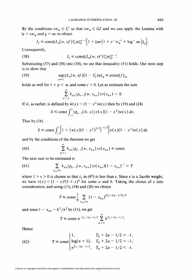
LAGRANGE INTERPOLATION. Ill 683
By the conditions vw^ E Lx so that vw^ E GJ and we can apply the Lemma with
'<f> = vwt and g = uv to obtain
72<const||Ln(w,o/)lc„M||£-1[l + ||hc(i + v~lw? + log+ «o)||J.
Consequently,
(58) 72<const||Ln(W,t>/)L>||£-1.
Substituting (57) and (58) into (54), we see that inequality (51) holds. Our next step
is to show that
(59) sup||L„(w, vf)(l - Vn)u\\p =s constH/IUn^X
holds as well for 1 < p < oo and some c > 0. Let us estimate the sum
n
2 ^kn\Pn-x(W>Xk„)\v(xkn) = S.k=X
If w, as earlier, is defined by w(x) — (1 — x2)w(x) then by (19) and (24)
S < const / \p„-x(w, x) \v(x)(l — x2)w(x) dx.J-x
Thus by (16)
•Mi
and by the conditions of the theorem we get
5^ const I'll + (w(x)(l - x2f/2y v(x)(l — x2)w(x) dx
(60) 2 XtB!/>„_,(w, xk„)\v(xk„)*z coast.k=\
The next sum to be estimated is
(61) 2 K»\Pn-i(w>xkn)\v{xk„)(\-xkn)~x = Txk„>e
where 1 > e > 0 is chosen so that tx in (47) is less than e. Since v is a Jacobi weight,
we have v(x) = (1 — x)"(l + x)b for some a and b. Taking the choice of e into
consideration, and using (11), (14) and (20) we obtain
rr^- 1 V t\ \(r0+2o-l/2)/2F=£ const- 2d (1 ~ xk„)
and since 1 — xkn ~ k /n by (11), we get
T< const «-r»"2a_,/2 2 kr°+2"-x/2.
k=\
Hence
1, r0 + 2a- 1/2 > -1,
log(«+l), r0 + 2a-l/2 = -l,
Br0-2«-i/2j Yo + 2a- 1/2 < -1.
(62) T < const
License or copyright restrictions may apply to redistribution; see http://www.ams.org/journal-terms-of-use

684 PAUL NEVAI
Now we turn to estimating Ln(w, vf,x) for 1 + xXn < 2x *£ 2. By (1) and (3) we
have
Ln(w,vf,x)\<2\\f\\xPn(x)1 "7 2 Xkn\Pn-x(W,Xkn)\v(xk„)
k=X
+ 2 Kn\Pn-i(w^ xk„)\v(xktt)(\ - xk„)'
1 + xXn < 2x< 2.
where e is chosen as in (61). Hence by (15) and (60)-(62)
'„r0+i/2| Y0 + 2a- 1/2 > -1,
«"2alog(«+ 1), r0 + 2a- 1/2 =-1,
«r»+1/2+ «-2a, r0 + 2a- 1/2 < -1,
\Ln(w, vf, x)\^ cons
for 1 + x,„ *S 2x < 2, and consequently
(63)
\L„(w, vf, *)|< const||/|| J«r°+1/2 + «-2alog(« +1)], 1 + x„, < 2* < 2.
If a > 0 then from (63) we get
\Ln(w, vf, x)\*í cons
and thus
(64) f \Ln(w,vf,x)u(x)\pdxJ(X+xu,)/2
1 + 1/i/w(jc)V1 ~*2 1 + x,„<2*<2,
cons tll/115,/(l+*l„)/2
1 +
]lw(x)xjl-x2
u(x)pdx.
If a *£0 then by (11) and (63)
|L„(w,i;/,x)|<const||/||c 1 + l/Jw(x)\jl - x: + t)(x)log(« + 1)],
1 + xx„ < 2x =s 2,
and consequently
\Ln(w,vf,x)u(x)\
<const||/||c u(x) + u(x)/]lw(x)\jl — X
1/2/7,+ 2pu(x)v(x)log+ u(x)v(x) + (n+ l)w plog(n + 1)
1 + xXn <2x <2.
License or copyright restrictions may apply to redistribution; see http://www.ams.org/journal-terms-of-use

LAGRANGE INTERPOLATION. Ill 685
Hence
(65)•i
f' \L„(w,vf,x)u(x)\p <consJ(l+xx„)/2
,/(i+*i.)/2
u(x) +u(x)
i/w(x)y 1 — xl
+ 2pu(x)v(x)log+ u(x)v(x) dx
+ (l-x,j2-'(«+l)'//(log(«+l))
Since by (11), 1 — xXn < const « , we obtain from (64) and (65) that-i
(66) / \Ln(w,vf)u p <const||/"!!£.
whenever w, v and u satisfy the conditions of the theorem. The inequality
f(-X+x„„)/2i(67)
t\Ln{w,vf)uf< cons
can be proved by similar arguments. Now let / be a singularity of w in (47) such that
j E t (see (48)), in another words let r be such that the corresponding T¡ is negative.
We will show that
(68) IL^w.o/.jOl^constll/IU, |x-fy|< l/n.
Let 8 > 0 be chosen so that tJ+x < tj - 28 < t} + 28 < t/_] with the notation
tm+x = -1 and r0 = 1. Then by (11) there exist a uniformly bounded number of
roots xkn such that | x — xkn |< 2/« if | x — t¡ |< 1/«. Hence
1/2
2 \lkn(x)\\x-xk^2/n
V A V ^kn\x)li Kkn L
\x-xk„\^2/n k=\ A¿«
2 hnK(x)'\x-xk¿<2/n
1/2
|x-/!<!/«,
and by (13)
(69) 2 |/¿„(x) |*£ const, \x-tj\<l/n.\x-x„„\*2/n
If |x - tj\< l/n and |x - xkn\> 2/n then \tj -xkn\<3\x- xkn\/2. Thus by (1),
(3), (14) and (15)
2 |Ux)|s£const«V2-' 2 \tj-xkn\V-x.2/n^\x-xkJ,<S 2/n<[x~xk„\^S
License or copyright restrictions may apply to redistribution; see http://www.ams.org/journal-terms-of-use

686 PAUL NEVAI
We can estimate | f — xkn | by (11) we obtain
/ \r'/2-l2 |Ux)|<œnst«V2->2(i)
2/n«|.ï-.\A„|«8 /=!
1
Since Tj < 0, we can conclude that
(70) 2 I/*„(*)!< const, \x-tj\<2//.«lx-.vt,J*8
Applying (1), (15) and (60) we see that
(71) 2 v(xkm)\ikH(x)\<coastnTj'2, \x-tj\<]-.»<lx-**J
By the choice of ô the function t> is uniformly bounded on [r ■ — 25, i- + 25] D [x —
5, x + 8] if |x - tj\< l/n. Because 1} < 0, we obtain from (69)-(71) that (68) holds,
and consequently
(72) fJ+V"\Ln(w, vf)u\» < const||/||£.
Now we choose 1 > c > 0 so that (-1 + x„„)/2 > -1 + c«"2, (1 + x,„)/2 < 1 -
en'2. The existence of such a number c is guaranteed by (11). Since t in (48) contains
no more than m indices, inequality (59) follows from (66), (67) and (72). For
1 < p < oo the theorem follows from (51) and (59). Now let 0 < p < 1. Define ü by
= up/2u — uI i—, \(p~¿)/¿
1 + Uwjl-x2 + t><2-"/2(l + (log+ vuf~p)/2)
Then ü ^ up/1 and ¿7 *s up/2(\Jw\fï~- x2 f2~p^2 so that w E L1 and
(VWl -x2V'm E L2. Moreover, vü < (vu)p/2 and u« *£ (u«)/,/2(log+ uk)^"2'72.
Thus u«log+ üü< (^/2)(ü«)''/2(log+ uuK/2 so that vü E L2(log+ L)2. Hence we
can apply (46) with p = 2 to obtain
||L„(ü/)I7||2<const||/||0C.
Since
(mû"1)2'7'2-'0 < 42/,A2"/')M^
■p
I + dw\}\ - x2 +vp + i^(log+ uu)
we have uu ' E L2^2 /'). By Holder's inequality
\\Ln(vf)u\\p < \\Ln(vf)ü\\2\\uü-x\\2pA2_p),
and consequently, the theorem also follows for 0 < p < 1.
Theorem 2. Let w E GSJ and 0 <p < oo. Let v be a not necessarily integrable
Jacobi weight function and let u be a measurable nonnegative function in [-1,1] such
that u is positive on a set with positive measure. Suppose that
(73) supllTjw.t/H^constH/ILn>\
License or copyright restrictions may apply to redistribution; see http://www.ams.org/journal-terms-of-use

LAGRANGE INTERPOLATION. Ill 687
for every continuous function f vanishing at ± 1. Then u E Lp, uv E Lp and
(74) vJwxjl - x2 E Lx and u/\lw\Jl - x2 E Lp.
Moreover, there exists a nonnegative u such that u E Lp, uv E Lp\(Llog+ L)p and
if (74) holds then (73) is not necessarily true for every continuous function vanishing at
±1,
Proof. It is obvious that u E Lp whenever (73) holds. In order to show that
uv E Lp as well as notice that if fv is continuous then by Erdos-Turán's L2 theorem
[6, p. 146]
lim||L„(w,ü/)-o/]H>||2 = 0«^ oc
so that there exists a subsequence {nk} such that
lim L„(w, vf, x) = u(x)/(x)*->oc
for almost every x in [-1,1]. By (73) supk>x\\Ln/(w, vf)u\\p < consty/H^ for such a
function/if f(± 1) = 0 and by Fatou's lemma
(75) llüMl^constll/IL
whenever fv is continuous and / vanishes at ±1. Now we choose a sequence (/}
such that fj(± 1) = 0, H/H^ ^ 1, /u E C[-l, 1] and /(x) -»y-«, 1 for every x £
(-1,1). Then by (75) supj>x\\fjvu\\p ^ const and another application of Fatou's
lemma yields uv E Lp. Now suppose that (73) holds but v\jw\J 1 — x2 is not
integrable. If w is given by (10) and v is defined by v(x) = (1 — x)"(l + x)*, then
this amounts to either a + T0/2 + 5/4 < 0 or b + Tm+ ,/2 + 5/4 < 0. Let 0 < e < 1
be chosen so that t x < e and -e < tm where tx and tm are given in (10). Then by (11),
(14) and (20)
2 Xkn\Pn-x(w, Xk„)\v(xkn)I**„I»f
\ 1 0+**„F+IW2+3/4 + 7 2 0-^)a+ro/2+3/4
xk„<-e xkn>e
1 / k \2* + T„,+ l+3/2 , I uy
n , " \ n I « "\n I
i, ^2ft+Tm+l+3/2 | j i, ^2a + r0 + 3/2
-and since either 2b + Tm+X + 3/2 < -1 or 2a + T0 + 3/2 < -1, we have
(76) lim 2 ^kn\Pn-x(w>xkn)\v(xkn) = ce.
Let {/„} be a sequence of continuous functions such that/„(± 1) = 0,fn(xkn) — 0 for
I**J<e»/„(■**«) = -sign/>„_,(w, xk„) fore^x^ 1, f„(xk„) = sign pn_x(w, xkn)
License or copyright restrictions may apply to redistribution; see http://www.ams.org/journal-terms-of-use

688 PAUL NEVAI
for -1 < xkn < -e and |/„(x)|< 1 for every x in [-1,1]. Using (3), we have
yLn(W' »/„. X) = -^/»„(W, X)
in2 Kn\Pm-l(*> Xk„)\v(xk„)(xk„ ~ x)
I
+ 2 *kn\Pn-AW'Xk„)\v(xk„)(x-Xk„yVa„<-f
and consequently
(77) \Ln(w,vfn,x)\>\^\pn(w,x)\ 2 r\kn\p„_x(w,xkn)\ü(xkn)
for |x |< e. Applying (21), (73), (76) and (77) we obtain
lim f\p„(w, x)u(x)f dx = 0n — oo J-t
and by [13, Theorem 4.2.8, p. 42] u(x) = 0 for almost every x in [-e, e]. Letting
e -> 1 we see that u must vanish almost everywhere in [-1,1] whenever vxjw^l — x2
is not integrable, and this contradicts to the conditions of the theorem. Now assume
that (73) holds whereas u/ ywVl ~~ xl does not belong to Lp. Then [13, Theorem
7.32, p. 138]
lim \\p„(w)u\\ = oo.«-•oc
Hence we can choose an interval A such that either A = [-1,0] or A = [0,1] and
(78) lim suplíp„(w)ulA|| = ooH-+ 00
where lá is the characteristic function of A. Let {/„} be a sequence of continuous
functions such that /„(±1) = 0, f„(xk„) = sign /?„_,(w, xkn) • [1 - l&(xk„)] and
|/,(x)|^ lfxxr-1 <x< 1. Then by (3)
Ln(w,vf„x)=^-Zlpn(w,x) 2 Xtn|/?B_,(w, xkn)\v(xkn)(x- xkn)~X
'" xkKe&
and therefore
I y _
\L„(w,vf„,x)\>--^-1\pn(w,x)\ 2 hkn\Pn-l(w>Xk„)\v(xkn)" xk„(£\
for x E A. Now we can apply (21), (73) and (78) to obtain
liminf 2 Xkn\Pn-x(w>xkn)\v(xk„) = 0.
Choose an interval A* such that A* n A = 0, ± 1 £ A* and if w is defined by (10)
then none of the singularities r of w belong to A*. Then
liminf 2 *kn\P«-i(w>xk„)\v(xk„) = 0.»-« ,vA„eA«
and by (20) \pn_x(w, xkn)\v(xk„) > const for xkn E A* so that
liminf 2 Xkn — 0-
License or copyright restrictions may apply to redistribution; see http://www.ams.org/journal-terms-of-use

LAGRANGE INTERPOLATION. Ill 689
By the quadrature convergence theorem [7, p. 89]
lim 2 A*„ = f
and consequently
' H' = 0
w-A*
/,■'A*
so that h(.y) = 0 for almost every x E A*. This contradiction shows that
«/ v'm'v 1 — x2 must belong to Lp whenever (73) is satisfied. In order to prove the
last part of the theorem we assume that if u E Lp, uv E Lp and (74) is satisfied then
(73) holds. First we fix an interval, say A, such that ± 1 E A and if w is defined by
(10) then none of the singularities t, of w belong to A. We will show that if/ is
continuous in [-1, 1] and/is supported in A then
(79) \xm\\{Ln(w,vf)-vf\u\\p = 0n -- oc
if (73) holds. Since vfis continuous in [-1,1] and vanishes outside A, for every 5 > 0
we can pick a polynomial R such that v(± l)"'/?(± 1) = 0 and |t;(x)/(x) — /?(x)|s£
5t>(x) for -1 < x < 1. Hence by (73)
\\[L„(w,vf)-vf]u\\p^const{\\[Ln(w,vf-R)]u\\p + \\[vf~R]u\\p}^const8
if « > deg /?. Therefore (79) is indeed true for continuous functions/supported in A
whenever (73) holds. Now let u be an arbitrary Lx function supported in A. By the
choice of A, if u =\u>\x/p then u E L", uv E Lp and u/ \Jwxfl - x2 E Lp so that
by the assumptions made
lim (\La(w,vf)-vf\'a = 0n-» oc •'A
for every continuous function / supported in A. Thus by the Banach-Steinhaus
theorem there exists a constant K, depending on/but independent of w such that
supnS-\
[\L„(w,vf)-vf\"u <Kf[\u\Jà
and taking the supremum of the left side over every u with /A | w |= 1 we obtain
(80) sup\\Ln(w,vf)-vf\\px<Kfn>\
where the oo-norm is taken over A, and / is an arbitrary continuous function
supported in A. Let C0(A) be the Banach space of all continuous functions
supported on A such that the norm is defined by the maximum norm. For every
F E C0(A) there exists a function / such that F = vf and / E C0(A). Hence (80)
becomes
sup||L„(w,F)-F||0C<^n»X
License or copyright restrictions may apply to redistribution; see http://www.ams.org/journal-terms-of-use

690 PAUL NEVAI
for every F E C0(A) where the oo-norm is taken over A. Thus by the uniform
boundedness theorem [9, p. 26]
(81) sup max \Ln(w, F, x) |=£ const max |F(x) |„3=1 .YEA .VGA
for every F E C0(A). Let A, C A and A2 C A, be proper closed subintervals of A
and A,, respectively. Let x E A2 be a root of pn+x(w) and let/ be the index of that
zero of pn(w) which is closest to x. Then by (11)
(82) \x-xkn\<amst\k-j\/n, x,„EA,,/c^/.
Let F E C0(A) be chosen so that F(xjn) = 0, F(xkn) = 0 for xk„ E A\A„ F(xkn) =
sign[/>„_,(w, x,„)(x - x,„)] for xk„ E A, and |F\t)[< 1 for t E A. Then by (3)
L„(w, F, x) = -^-/»„(w, x) 2 XAn|/?B_,(w, xk„){x-xkn)~l\
*#/
and by (14), (20), (21) and (82)
|L„(w,F,x)|> const 2 \k~jV-
*#/Since by (11) the number of zeros xkn in A, is greater than const • «, we obtain
(83) \L„(w,F,x)\> const-log n.
Substituting (83) into (81) we get log« < const and since n can be as large as we
wish, we see that (73) cannot be true for every u satisfying u E Lp, uv E Lp and
(74). The proof of the theorem has been completed.
Theorem 3. Let w, v, u andp satisfy the conditions of Theorem 1. Suppose that
(84) lim||[Zjw,t>)-t>]«||, = 0.
Then for every continuous function f in [-1,1] we also have
(85) lim||[L„(W,O/)-u/]ii||, = 0.n-* oc
Proof. By Theorem 1 we have to show that (85) holds when/is a polynomial. By
linearity we can assume that / is of the form f(x) = x' where / is a nonnegative
integer. Since we assume that (84) holds, we only have to prove (85) for / > 1. If
f(x) =x',l> 1, then
L,,(w, vf) -vf= L„(w, vf) -fLn(w, v) +f[L,,(w, v) - v]
and by (84) formula (85) holds if
(86) lim ||[L„(w, vf) ~fLn(w, v)]u\\p = 0.n —oo
Hence our goal is to prove (86). We have
n
L„(w,vf,x)-f(x)L„{w,v,x)= 2 [x'kn- x']v(xkn)lk„(w,x)k=X
l-X n
= - 2 x'~x~J 2 (x - xk„)x(„v(xk„)lk„(w, x).7 = 0 *=1
License or copyright restrictions may apply to redistribution; see http://www.ams.org/journal-terms-of-use

LAGRANGE INTERPOLATION. Ill 691
Applying (3) we get
(87)
_ y»-12 (X-Xk„)xí„v{xkn)lkn(w,x)= -^Pniw, X) 2 XÍ„v(xk„)p„_x(w, Xk„)\k„.
k=X y„ k=X
Thus by (1), (16) and (87)
(88) ||L„(w, vf) -fLn(w, v)\u\\. < const 1 +Wl — X1
max0=S;«/-1
2 x{nv{xkn)pn_x{w,xkn)Xknk=X
so that (86) holds if
(89) lim 2 xJknv(xk„)pn-](w,xkn)\kn = 0, j = 0,l,....n-00 k=]
Let 0 < e < 1 be chosen so that all the singularities tk of w in (10) belong to [-e, e]. If
R is an arbitrary polynomial and « > deg 7? + 1 then by the Gauss-Jacobi quadra-
ture formula
n
2 Hxkn)pn_x(w,xkn)Xkn = 0.k = X
Let lf be the characteristic function of [-e, e]. Then
n
2 y(xkn)xinv(xk„)pn_x(w,xkn)\kn
k=X
= 2 bc(xkn)xJknv(xkn) - R(xk„)]p„_x(w, xkn)\kn.k=X
Applying Cauchy's inequality we obtain
(90)* = i2 \Áxkn)x{nv(xkn)pn_x(w, xkn)\kn
n n
2 X*« 2 [lÁxkn)xLv(xk„) - R(xkn)]2Pn_x(w, Xkn)2\k„.k=X k=X
By the Gauss-Jacobi quadrature formula
n
2 ̂ knk=X
Since [1ex7ü - 7?]2 is Riemann integrable, by [13, Theorem 4.2.3, p. 39] the second
sum on the right side of (90) converges as « -» oo, and evaluating its limit by the
License or copyright restrictions may apply to redistribution; see http://www.ams.org/journal-terms-of-use

692 PAUL NEVAI
same theorem we obtain
lim supn— oo
2 y(xk„)xJknv(xkn)pn_x(w, xkn)Xklk=X
2 t\< -\w\xf_[y(<)'jv(t) - R{t)]2x¡i -12 dt
and taking the infimum on the right side here with respect to R we get
/<•
(91) lim % lf(xk„)xl„v(xk„)p„_f(w,xk„)\k„ = 0, ./= 0.1."-* *=i
We have
2 xi„v(xk„)p„_x(w,xk„)\k„l-Vt„|3=F
2 v(xk„)\p„ ,(w, xk„)\\kH
and by (14) and (20)
(92)
2 xi„v(xk„)p„-x{w, xk„)\kn const 2 v(xkn)\Jw(xk„) (l - x\„)3/4
« |.Vt„pF
Since v is a Jacobi weight, w behaves like a Jacobi weight on [-1,-e] U [e, 1] and
vywy/l ~~ x2 E Ü, there exists a number 5 > -1 such that
v(xk„)]/w(xkn)(l - x2„)3/4 *£ const(l - x2„) /
and by(11)
.2 \3/4^_ i(*/«)',(93) y(xA,,)v/w(xA.„)(l -x¿„) ^ const
k*n -e,
[((«+ 1 -£)/«) , l*n
Also by (11) if xkn > e then 1 < k < const^l — e2 • « and if xkn < -e then 1 «£ « +
1 - k « constv7! - e2 ■ n. Thus by (92) and (93)
(94) 2 x{„v(xkn)pn_x{w,xkn)\kn
l-ÏA„l»F
<const(5+ 1) (1 -e2)2\(S+')/2
Combining (91) and (94) we obtain
n
limsup 2 x(„v(xkn)pn_x(w,xk„)Xknn — oo * = 1
const(5 + 1) (1 -e2)2\(«+')/2
and letting e -> 1 formula (89) follows and so does (86).
Theorem 4. Let w E GSJ and 0 < p < oo. Let v be a not necessarily integrable
rational Jacobi weight function, and let u be a nonnegative function supported in [-1, 1]
such that uE Lp,uv E Lp,u/ yWl - x2 EL" and uyWl - x2 E Ü. Then
(95) lim ||[Z.„(W,ü)-ü]tt|| =0.
License or copyright restrictions may apply to redistribution; see http://www.ams.org/journal-terms-of-use

LAGRANGE INTERPOLATION. Ill 693
Proof. Let v(x) = (1 — x)a(l + x)h where a and b are integers. If a > 0 and
6 s= 0 then o is a polynomial and thus (95) holds. If a < 0 and b s* 0 then we
proceed as follows. Choosing « > b we see that
(1 - x)""[L„(w, t),x) - t>(x)]
is a polynomial of degree -a + « — 1 vanishing at the zeros of p„(w, x). Hence there
exists a polynomial R_a x of degree -a — 1 such that
(1 - xya[Ln(w, v,x) - v(x)] =pn(w,x)R_a_x{x).
The polynomial 7?_a_, can explictly be determined by dividing both sides by p„(w),
expanding them in powers of (x — 1) and noticing than (1 — x)~"Ln(w, v, x) has a
zero at 1 with multiplicity at least -a. Proceeding this way we obtain
(96)
-a-]
L„(w, v,x) -v(x) = (1 -x)"pn(w, x) 2 (-1)'+1 = 0
/!
(i + 0ft
p,Xw^)
(/)
(I-*)'.I 1
If w is given by ( 10) then, since v\J wyl L), we have 5 = 2a + ro + 5/2 > 0.
Let e be chosen so that tx < e < 1 where tx is defined in (10). Since a < -1, F0 must
be greater than -1/2 and thus by (15),
\p„(w,x)\(l -x)'< const (1 - x)'/\jw(x)\jl - x2 , e < x *S 1,
I = 0,l,...,a — I. Applying (26) we obtain
(97) \p,,(w,x)\(l -x)'< const «-2//|/w(l - «"2)V«_2 « const „-2/+r<>+1/2,
E<X< 1,
/ = 0, 1,..., -a - 1. It follows from (17) and (23) that
(98)(1 + 0'
(0
i i
const « 2/-r0-i/2
A,(w>0
for / = 0,1,..., -a - 1. Combining (96)-(98) we get
(99) \L„{w, v, x) - ü(x)|=£ const v(x), e =s x
For -1 ^i<£we can apply (16), (96) and (98) to obtain
(100) \Ln(w, v, x) - u(x)|< const
1.
l/i/w(xVl -x2 + 1 1 e,
where 5 > 0. Now (95) follows immediately from (99) and (100). If a > 0 and b < 0
then we can use similar arguments to prove (95). If both a and b are negative, then
v~x[Ln(w, v) — v] is a polynomial of degree -a — b + n — I which vanishes at zeros
License or copyright restrictions may apply to redistribution; see http://www.ams.org/journal-terms-of-use

694 PAUL NEVAI
of p„(w). Using the Hermite interpolation formula we obtain
(101)
-a-1 1L„(w,v,x)-v(x) = (l - x)"pn(w,x) 2 (-0'+1Tj
/=0
b-X
(1 + x)'pn(w,x) 2 77/=0
(i + O*/>„(*'• 0
(i-0a1(/)
(/)(1-x)'
r= i
(1+x)'.
Choosing e so that r, < e < 1 and -1 < -e < tm (see (10)) we get that both (97) and
(98) hold and by similar arguments we obtain
(102) \p„(w, x)\(l + x)'< const n-2l+r»'+< + x/2, -I < x <-e,
and
(103)
(i-0a
Pn(W't)
(/)
r=-l
const n 2/-r„1+1-i/2 1 ^X *£ -E,
for / = 0, l,...,-b - 1. Since vxjwjl - x2=~ E Lx we get that both 8 = 2a + T0 +
5/2 and 5, = 2b + Ym+X + 5/2 are positive. Now from (97), (98) and (101)-(103)
we obtain
o(x) + «-Ä'/i/tv(xWl -x2 , e<x<l,
il + l/xjw(x){ï^2\(n-s + «-«■),
-£ < x «S e,
v(x) + n-s/xlw(x)'Jl -x2', -l<x<-e,
\Ln(w, v, x) — ü(x)|*£ const
and the theorem follows again.
Theorem 5. Let w E GSJ, 0 < p < oo and let v be a not necessarily integrable
Jacobi weight, say v(x) = (1 - x)a(l + x)* for |x|< 1. Let v* be a rational Jacobi
weight defined by v*(x) = (1 - x)[al(l + x)'*1 for |x|< 1. If u is a nonnegative
function supported in [-1,1] and u E Lp, uv* E (Llog+ L)p, u/ xjwy/l — x2 E Lp
andv*xjw\jl - x2 E Lx then
(104) lim||[L„Ku/)-o/]ii||, = 0«-»00
holds for every continuous function f in [-1,1].
Proof. By Theorems 3 and 4 we have
(105) lim\\[Ln(w,v*F)-v*F]u\\ = 0//-* oc
for every F E C[-l, 1] and by the construction of v* the function F = v(v*)'xf is
continuous whenever/is continuous. Thus (104) holds by (105).
License or copyright restrictions may apply to redistribution; see http://www.ams.org/journal-terms-of-use

LAGRANGE INTERPOLATION. Ill 695
Theorem 6. Let w E GSJ, 0 < p < oo, and let r and s be nonnegative integers. Let
u be a nonnegative function defined in [-1,1] such that u E (Llog+ L)p and u is
positive on a set with positive measure. Let L[r,s)(w, f) be the quasi-Lagrange
interpolating polynomial defined by (5)-(8) and let v(x) = (1 — x)~r(l + x)~v. Then
(106) hm||[L<-»(w,/)-/]M||/J = 0, V/EC[-1,1],
holds if and only if
vJwxJl - x2 E l) and u/ vJwxJl - x2 E Lp.(107)
Moreover, there exists a nonnegative u such that u E Lp\(Llog+ Lp) and (107) does
not imply (106).
Proof. We start with writing L(nr-S)(w, f) in the form
(108) L^\w, f) = v~xLn(w,vf) + f(l)Q + f(-l)R
where
(109) Q(x) = (l+xyPn(w,x)'Z(-iy-[\
and
1=0
1
i-i(no) /?(x) = (i-x)»,x)2 77
/ = 0
a(w, 0(i + 0'
(/)
(i»0-x)'
p„(w,t)(l-t)r(l+x)1.
If either r or i equals 0 then the corresponding polynomial Q or 7? is identically 0.
(108)-(110) follow immediately from (5)-(8). If (106) holds then by the uniform
boundedness principle [13, p. 182]
(HI) sup||4^(w, /)«|| ^constll/IL
for every/ E C[-l, 1], in particular, if f(± 1) = 0. Thus by (108)
sup||L„(w, vf)v-]u\\p ^ constll/H««s=l
for every continuous function / vanishing at ± 1. Applying Theorem 2 we see that
conditions (107) are satisfied. Conversely, if (107) holds then by Theorem 5
(112) lim \\[Ln(w,vF) -vF]v-]u\\p = 0n-> oc
for every F E. C[-l, 1]. For/ E C[-l, 1] let P be any fixed polynomial satisfying
P(t)U)\1=x=f(l)80j, 0<j<r-l,
and
P(t)U)\!=_xf(-l)80j, 0<j<s-l.
If r + s + « - 1 ̂ deg P then
S„ = v-]L„(w,(f- P)v) + P- L^(w, f)
License or copyright restrictions may apply to redistribution; see http://www.ams.org/journal-terms-of-use

696 PAUL NEVAI
is a polynomial of degree r + s + « — 1 satisfying
Sn(xk„(w)) = 0, 1 <*</!,
Sn(0O)|/=1=0, 0</<r-l,
and
^,(0O)U-, = o, o</«s-i,
so that S„ is identically 0. Thus
ü;-*\w, f) = v-lLn(w,(f- P)v) + P
and if F is defined by F = f — P then
L\;-\w, f) - f = v-'[L„(w,vF) - vF\.
Hence by (112), (106) is true for every / E C[-l, 1]. Now we turn to the last part of
the theorem. Suppose that for every nonnegative u E Lp satisfying (107), (106)
holds. Then (111) holds as well, and by (108)
(113) sup||L„(w,ü/)ü-,W||/7<const||/||x•is-1
is satisfied for every continuous function / vanishing at ± 1. But according to
Theorem 2, (113) fails for some u E Lp and some/E G[-l, 1] with/(± 1) = 0. This
shows that (106) cannot be true for every u E Lp when (107) holds.
Partial cases of Theorem 6 have been proved in [1,2,5,6,10,11,14 and 19].
Even though it is unlikely that uv must belong to (Llog+ L)p whenever (73) holds
for every continuous function /, the following theorem demonstrates that this, in
fact, is not too far from the truth.
Theorem 7. Let w E GSJ and 0 < p < oo. Suppose that either
(114) 0< limw(x)\/l - x2 < oo.Y-> 1
or
(115) 0< lim w(x){l~^x2 < oox — -1
holds. Then there exists a nonnegative function u with support in [-1,1] such that
u/ xjwyjl — x2 E Lp and u E Lp(log+ L)q for every q <p and nevertheless
(116) sup sup \\Ln(w,f)u\\p= oo.«»i ll/lloc«.
fee
Proof. Assume without loss of generality that (114) holds. Pick e such that
0 < e < 1 and
(117) w(x)\Jl - x2 ~ 1, £=e:x=£1
is satisfied. Let lf be the characteristic function of [e, 1]. Define u by
(118) u(x) = l£(x)(l -x)-x/p\\og(\ -x)r1-'/*|log|log(l-x)||,/>.
License or copyright restrictions may apply to redistribution; see http://www.ams.org/journal-terms-of-use

LAGRANGEINTERPOLATION.III 697
Then u E Lp so that by (117) u/ yWl ~~ x2 E Lp as well. If q < p then, since
(log+ h(x))?=£ const lf(x)|log(l -x)f, |x|< 1,
we have
u(x)p(log+ w(x))"< const l£(x)(l -x)"'|k>g(l - x) \"-p-] | log j log( 1 -x)||
and hence u E Lp(log+ L)q. Now choose c > 0 such that 1 - en'2 > {(I + xXn(w))
holds for every «EN. This can be accomplished by (11). If « is large enough then
Ç \u(x)\pdx>constloglognC (1 - x)"' |log(l - x) \-"-] dxJX-cn~2 JX-cn-2
> const log log « • (log n)'p,
and consequently
(119) sup (log «)"/"' \u(x)\pdx= oo.n^X J\-cn~2
For every « pick a continuous function/, such that f„(xkn) = sign /?„_,( w, xkn) for
e *£ xk„ < l,f,(xkn) = 0 forx,,, < e and |/„(x)|« 1 for |*|< 1. Then
L„(w,/„,x) = 2 I4>^)l. i-«r2<x*:l,
and by (3), ( 11 ), ( 14), (20) and (21 )
(120) Ln(w, /,, x) > const log npn(w, x), I c«~2<x*£l.
The next step is to show that
(121) pn(w, x) s* const, 1 - or2 =sx=s 1.
We have
^^- n^^= nfi-71-^)^ n (i--*^^A,^. O *=,1~**« k = x\ 1_**J k=x\ 2(1 -xkn))'
1 - c«"2 *£x< 1,
since 1 - e«-2 3= j-(l + x,„). But log(l - x)> -2x for 0 =£ x < A. Thus
^*> > exp (i-*.„)2*=1 ] Xk"/>„(*> 0
= exp[-(l -xln)pn(w,l)>„(H',l)"1], 1 -c«-2«x=£ 1.
Now (121) follows from (11), (17) and (22). We obtain from (120) and (121) that
(' |L>,/>|'>const(logn)i'/'1 |«|>Ji-cn~2 JX-cn~2
and by (119) we see that (116) holds when u is defined by (118).
References
1. R. Askey, Mean convergence of orthogonal series and Lagrange interpolation. Acta Math. Acad. Sei.
Hungar. 23(1972), 71-85.
2._, Summability of Jacobi series, Trans. Amer. Math. Soc. 179 (1973), 71-84.
3. V. Badkov, Convergence in the mean and almost everywhere of Fourier series in polynomials
orthogonal on an interval, Math. USSR-Sb. 24 (1974), 223-256.
License or copyright restrictions may apply to redistribution; see http://www.ams.org/journal-terms-of-use

698 PAUL NEVA!
4. N. Dunford and J. T. Schwartz, Linear operators. Vol. 2, Interscience, New York, 1958.
5. P. Erdös and E. Feldheim, Sur le mode de convergence pour l'interpolation de Lagrange, C. R. Acad.
Sei. Paris Ser. A-B 203 (1936), 913-915.
6. P. Erdös and P. Turan, On interpolation. I, II, III, Ann. of Math. 38 (1937), 142-151; 39 (1938),703-724:41(1940), 510-553.
7. G. Freud, Orthogonal polynomials, Pergamon Press, New York, 1971.
8. _, Über eine Klasse Lagrangeseher Interpolationsverfahren, Studia Sei. Math. Hungar. 3
(1968), 249-255.9. E. Hille and R. S. Phillips, Functional analysis and semigroups, Amer. Math. Soc. Colloq. Publ., vol.
31, Amer. Math. Soc., Providence, R. L, 1957.
10. M. Kuetz, A note on mean convergence of Lagrange interpolation, J. Approx. Theory 35 (1982),
77-82.U.J. Marcinkiewicz, Sur l'interpolation. I, Studia Math. 6 ( 1936), 1-17.
12. I. P. Natanson, Constructive function theory, Vol. 1, Ungar. New York, 1964.
13. P. Nevai, Orthogonal polynomials, Mem. Amer. Math. Soc. no. 213, 1979.
14. _, Mean convergence of Lagrange interpolation. I. II, J. Approx. Theory 18 (1976), 363-377;
30(1980),263-276.15._Lagrange interpolation at zeros of orthogonal polynomials. Approximation Theory. II (G. G.
Lorentz et al., eds.). Academic Press, New York, 1976, pp. 163-201.
16. P. Nevai and P. Vértesi, Mean convergence of Hermite-Fejér interpolation, J. Math. Anal. Appl. (to
appear).
17. E. Stein, Singular integrals and differentiability properties of functions, Princeton Univ. Press,
Princeton, N. J., 1970.
18. G. Szegö, Orthogonal polynomials. Amer. Math. Soc. Colloq. Publ., vol. 23. Amer. Math. Soc.,
Providence, R. I., 1967.
19. A. K. Varma and P. Vértesi, some Erdös-Feldheim type theorems on mean convergence of Lagrange
interpolation, J. Math. Anal. Appl. 91 (1983), 68-79.20. P. Vértesi, Remarks on the Lagrange interpolation, Studia Sei. Math. Hungar. 15 (1980). 277-281.
Department of Mathematics, Ohio State University, Columbus, Ohio 43210
License or copyright restrictions may apply to redistribution; see http://www.ams.org/journal-terms-of-use


![Interpolation & Polynomial Approximation [0.125in]3.625in0 ...mamu/courses/231/Slides/CH03_1A.pdf · Interpolation & Polynomial Approximation Lagrange Interpolating Polynomials I](https://static.fdocuments.in/doc/165x107/5d2dac6988c99309368c7428/interpolation-polynomial-approximation-0125in3625in0-mamucourses231slidesch031apdf.jpg)
![MEAN CONVERGENCE OF LAGRANGE INTERPOLATION. Ill...convergence of Lagrange interpolation, we suggest [1,14 and 15] as references. An application of the results of this paper to weighted](https://static.fdocuments.in/doc/165x107/606d634e42fc64173a1be3f7/mean-convergence-of-lagrange-interpolation-ill-convergence-of-lagrange-interpolation.jpg)